LR-WaveHoltz: A Low-Rank Helmholtz Solver

We consider a smooth open domain $\Omega\subset\mathbb{R}^{d}$ which is assumed to either be fully submerged under water or have its top boundary as the water surface. The problem is driven by a forcing $f({\mathbf{x}})$, has a potentially discontinuously varying wave speed $c$ and a damping $\kappa({\mathbf{x}})$. We are interested in the distribution of the acoustic pressure $u({\mathbf{x}})$ generated by a forcing oscillating at a given frequency $\omega$, which is modeled by the Helmholtz equation [20]

where $a,b$ are constants satisfying $a^{2}+b^{2}=1$. The boundary conditions (3) model the lowest order nonreflecting boundary conditions when $a,b=\frac{1}{\sqrt{2}}$.

Extensions of the model could take higher order nonreflecting boundary conditions [17] and acoustic-elastic interaction with the sea floor [6] into account.

We briefly summarize the WaveHoltz method developed in [5]. Introducing the $T=\frac{2\pi}{\omega}$-periodic function $w=w({\mathbf{x}},t)=e^{i\omega t}u({\mathbf{x}})$, the associated wave problem of (2)-(3) is then given by

where $v_{0}({\mathbf{x}})=u({\mathbf{x}})$ and $v_{1}({\mathbf{x}})=i\omega u({\mathbf{x}})$. Assuming that the initial data of the wave problem satisfies $v_{0}\in H^{1}(\Omega)$ and $v_{1}\in L^{2}(\Omega)$, the WaveHoltz (WH) operator $\Pi$ acting on the data is defined as

The kernel in $\Pi$ is chosen to damp the frequencies away from $\omega$, while exactly preserving the $\omega$ mode. Applying this operator can therefore be viewed as a filtering of frequencies around $\omega$. Evaluating the integral in (5) results in $[u(x),i\omega u({\mathbf{x}})]^{T}$, hence the Helmholtz solution $u({\mathbf{x}})$ solves the fixed point problem $\Pi[u({\mathbf{x}}),i\omega u({\mathbf{x}})]^{T}=[u(x),i\omega u(x)]^{T}$. The WaveHoltz method is then the fixed point iteration

The convergence of the WaveHoltz method has been studied in [5, 31] where it was shown that under natural assumptions the iteration converges to the Helmholtz solution, i.e. $u=\lim_{n\rightarrow\infty}v^{(n)}$. It is expected that the number of iterations to converge grows like $\mathcal{O}(\omega)$, discussed in the context of impedance boundary conditions in [31].

As demonstrated in [5] and [31], the WaveHoltz iterations can be accelerated using a Krylov subspace method. One such method suitable for our low-rank formulation is Anderson acceleration (AA). Following the notation in [34], let $G:\mathcal{X}\rightarrow\mathcal{X}$ for some Hilbert space $\mathcal{X}\subset L^{2}(\Omega)$, $X\in\mathcal{X}$ and consider the fixed point problem $G(X)=X$. This is commonly solved using Picard iteration; given some initial condition $X^{0}\in\mathcal{X}$, update the iterates using

until convergence. Picard iteration only uses information from the previous iterate and converges conditionally. Moreover, the convergence is typically linear. To accelerate the convergence, AA instead uses a linear combination of a given number of previous iterates. More precisely, given a memory parameter or window size $m$, the iterate $X^{k}$ of the $\operatorname{AA}(m)$ method will use the previous $\min(m,k)+1$ iterates, outlined in Algorithm 1. From this definition we can infer that $\operatorname{AA}(0)$ corresponds to Picard iteration.

Note that $\|\cdot\|$ denotes a general norm in [34], but we resort to the Frobenius norm. The naive way of solving for the coefficients $\boldsymbol{\gamma}^{(k)}$ when $X^{k}\in\mathbb{R}^{n\times n}$ in (7) requires solving a large system of linear equations of size $\mathcal{O}(mn^{2})$ at each iteration. We reformulate the minimization problem in terms of a smaller system of the size $\mathcal{O}(m^{2})$ in Problem 2.1.

Let $I=[0,1]$ denote a one-dimensional interval discretized uniformly into $n$ gridpoints $\{x_{i}\}$ with grid spacing $h$ such that $x_{i}=(i-1)h$ and $h=\frac{1}{n-1}$. Moreover, let $u$ and $v$ be functions defined on $I$ with sufficient regularity, denoting the evaluation at a point $x_{i}$ as $u_{i}=u(x_{i}),v_{i}=v(x_{i})$ and grid evaluations as ${\mathbf{u}}=[u_{1},...,u_{n}]^{T},{\mathbf{v}}=[v_{1},...,v_{n}]^{T}$. We introduce the notion of narrow-stencil SBP operators $D_{1}\approx\partial_{x}$ and $D_{2}\approx\partial_{x}^{2}$ having order of accuracy $\mathcal{O}(h^{2p})$ in the interior and $\mathcal{O}(h^{p})$ at a few points near the boundary. The decreased order of accuracy is due to the one-sided stencil and we use the name convention that the operators are of order $2p$. We can then define the SBP property of the operators $D_{1}$ and $D_{2}$ [26].

The matrix $H$ defines a quadrature such that ${\mathbf{u}}^{T}H{\mathbf{v}}\approx\int_{I}u(x)v(x)dx$ and an associated inner product [18]. It should also be noted that the boundary derivative approximations have an improved order of accuracy $\mathcal{O}(h^{p+1})$ compared with $D_{1}$.

To discretize in space, we resort to the method outlined in [24], representing the numerical solution in each block as a matrix rather than a vector. For ease of presentation we restrict ourselves to a two-block domain with aligning grids, but the framework readily extends to a multiblock setting. Let $\Omega\subset\mathbb{R}^{2}$ with be a Cartesian domain, with coordinates $(x_{1},x_{2})\in\Omega$, partitioned into two subdomains $\Omega_{u}$ and $\Omega_{v}$ having a vertical interface $\Gamma=\partial\Omega_{u}\cap\partial\Omega_{v}$ at $x_{1}=0$ and constant, but not necessary equal, associated wave speeds $c_{u}$ and $c_{v}$. Furthermore, we denote the positive outward unit normal along $\partial\Omega$ as ${\mathbf{n}}$. The continuous problem in $\Omega$ can then be formulated as

where letters in the subscripts denote the domains. The solution and its normal flux across the interface must be continuous. Letting ${\mathbf{n}}_{\Gamma}$ denote the unit normal ${\mathbf{n}}_{\Gamma}=[1,0]^{T}$ at $\Gamma$, we formulate these conditions in terms of $u$ and $v$ as

We now turn to the SBP-SAT semidiscretization of the problem. Assume that the domains are Cartesian blocks discretized by $n$ degrees of freedom ${\mathbf{x}},{\mathbf{y}}\in\mathbb{R}^{n}$ in each direction. Then, we represent the time dependent grid evaluation of $u,v$ in each block as matrices $\mathbb{U}(t),\mathbb{V}(t)\in\mathbb{R}^{n\times n}$ ordered such that $\mathbb{U}_{ij}(t)=u(x_{i},y_{j},t)$ and $\mathbb{V}_{ij}(t)=v(x_{i},y_{j},t)$. Similarly, let $F_{u},F_{v}\in\mathbb{R}^{n\times n}$ denote the grid evaluations of the forcing $f(x,y)$ in the corresponding block. We use the difference operators defined in the previous section to approximate spatial derivatives as $\partial_{x}^{2}u(t)\approx D_{2}\mathbb{U}(t)$ and $\partial_{y}^{2}u(t)\approx\mathbb{U}(t)D_{2}^{T}$. The semidiscretization is then given by

where the first two terms approximate the Laplacian, the sum over SAT terms $\mathcal{S}^{u}_{i}(\mathbb{U},\mathbb{V}),\mathcal{S}^{v}_{i}(\mathbb{U},\mathbb{V})$ enforces interface or boundary conditions and the last term is the periodic forcing function. The indices of the SAT terms are ordered to represent different boundaries of the respective block, where the order is given as west, north, south and east. We present two of the SAT terms in the domain $\Omega_{u}$ as the remaining terms are constructed analogously. At the northern boundary, the nonreflecting condition $u_{t}+c_{u}\nabla u\cdot{\mathbf{n}}=0$ with ${\mathbf{n}}=[0,1]^{T}$ is imposed weakly by the term $\mathcal{S}_{2}^{u}(\mathbb{U},\mathbb{V})$ defined by

where we recall the definition of $H,S$ and ${\mathbf{e}}_{n}$ from section 3.1. Again, note that the operators act from the right on $\mathbb{U}$ as the boundary condition is in the vertical direction. Since the grid within the blocks are assumed to align, we impose the interface conditions (9)-(10) weakly along $\Gamma$, following the method outlined in [24]. If the mesh size is different in the two blocks, which might be desireable when the wave speed varies between the blocks, we can use the standard SBP projection approach from [1]. In $\Omega_{u}$, the interface conditions are imposed by the SAT term $\mathcal{S}_{4}(\mathbb{U},\mathbb{V})$

where $\tau>0$ denotes a stability parameter independent of wave speeds chosen suitably large depending on the order of the SBP method used, and $c_{av}=\frac{c_{u}^{2}+c_{v}^{2}}{2}$ [24]. Since the semi discretization is a matrix formulation of the method presented in [24] their stability result also applies here. It therefore follows that (11)-(12) satisfies an energy estimate when choosing $\tau$ sufficiently large.

Let $W(t)\in\mathbb{R}^{n\times n}$ denote the grid evaluation of a function $w$. We consider a general problem on the form

for some right-hand side $G(\cdot,\cdot)\in\mathbb{R}^{n\times n}$ being linear in its first argument. Denote the discrete solution to (14) at time $t^{k}$ by $W^{k}$ and let its singular value decomposition (SVD) be given as $W^{k}=U^{k}S^{k}(V^{k})^{T}$, where $U^{k}\in\mathbb{R}^{n\times r},S^{k}\in\mathbb{R}^{r\times r},V^{k}\in\mathbb{R}^{n\times r}$ for some $r>0$ denoting the rank of $W^{k}$. We introduce the truncated SVD operator $\mathcal{T}_{\epsilon}$ which approximates $W^{k}$ within a given accuracy $\epsilon$ as $\|W^{k}-\mathcal{T}_{\epsilon}(W^{k})\|<\epsilon$ where $\|\cdot\|$ denotes the Frobenius norm. The truncation tolerance $\epsilon$ is chosen such that the residual at the final iteration does not exceed the local truncation error of the underlying spatial discretization. The notation $\mathcal{T}_{\epsilon}(W^{k})$ should be understood as the operator acting on the SVD factors of $W^{k}$.

When we discretize (14) we will add up several terms at each time step. This addition will introduce rank growth. The problems we are targeting are assumed to have low rank at all times, we therefore need a summation operation $\mathcal{T}_{\epsilon}^{sum}$ mimicking the properties of $\mathcal{T}_{\epsilon}$, summarized in Algorithm 2 using MATLAB notation. We note that if the number of summands is large, the algorithm can be made more efficient by making it sequential. However, since we only have a few terms in the time discretization, we use the algorithm as presented.

We resort to second order centered differences to discretize (14) in time, resulting in (19) and present the evolution of one time step in Algorithm 3. The first step of the method consists of a regular leapfrog step for (14) with a truncated right hand side, yielding a solution $\widetilde{W}^{k+1}$ which may have a larger rank than desired. The second step then consists of truncating the sum in the first step using the summation operator $\mathcal{T}_{\epsilon}^{sum}(\cdot)$ described in Algorithm 2.

We now generalize the discretization of the domain $\Omega$ used in Section 3.1 to a general multiblock setting. For notational convenience, we assume that $\Omega$ is partitioned into $m$ blocks $\Omega_{ij}$ in each direction, where the subscripts from now on do not denote elements, but rather the indices of a block. The blocks are then discretized with $n$ gridpoints and grid size $h$ in each dimension. We denote the grid evaluation of the acoustic pressure $w$ and velocity $w^{\prime}$ in each block as the matrices $W_{ij}(t),W^{\prime}_{ij}(t)\in\mathbb{R}^{n\times n}$ for $i,j=1,\ldots,m$. We also need the operator $L_{ij}(W_{ij})\in\mathbb{R}^{n\times n}$ , referred to as the discrete Laplacian, combining $D_{2}W_{ij}+W_{ij}D_{2}^{T}$ with the factors from SAT-terms imposing boundary and interface conditions on $\partial\Omega_{ij}$. An illustration of the contributing edges is shown in Figure 1(a). The main idea is that given initial data in SVD form, we construct a scheme that retains the low-rank structure of the solution at all iterations, without ever having to form the full matrix. This can be done in a straightforward manner following the semidiscretization shown in (11)-(12) where the discrete Laplacian operates on the left or right singular vectors of the numerical solution. We present the solver in Algorithm 4 for a time interval $[0,T]$ discretized with time step $\Delta t$ and discuss it further below.

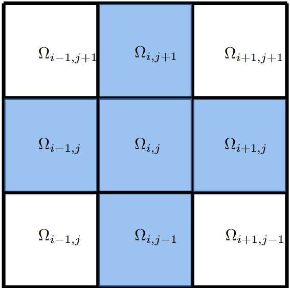
The method follows a standard wave solver using the leapfrog scheme in time, with the difference being the need of applying the truncation operators. We again stress that the notation $W_{ij}^{k},W_{ij}^{\prime}$ and $F_{ij}^{k}$ should be understood as in SVD form and all operations are done on the factors of the solution and never on the full matrix. The first step of the method consists of the usual construction of the solution at time $-\Delta t$ required for leapfrog method. Then, looping over each block, we first compute $\widehat{W}^{k+1}_{ij}$, consisting of the discrete Laplacian and forcing term. We then add the contribution from the second derivative to form $\widetilde{W}^{k+1}_{ij}$ and round with an overall tolerance of $\epsilon$.

We now consider the terms arising from $W^{\prime}(t)$ in the nonreflecting boundary conditions. Consider the corner block in Figure 1(b). For notational convenience, let $c$ denote the wave speed in this multiblock. When $W^{k+1}_{ij}$-terms are combined we obtain

where the matrix $R$ depends on $W^{k}_{ij}$ and $W^{k-1}_{ij}$. A difference compared to vectorized formulations is now that $W^{k+1}_{ij}$ cannot be obtained by a straightforward linear solve. Instead, we have to solve a matrix equation. To this end, we recast the problem into a Sylvester equation $AW^{k+1}_{ij}-W^{k+1}_{ij}B^{T}=R$, which we then solve using the factored Alternating Direction Iteration [9]. In this context fADI converges in exactly three iterations. This method is particularly useful as the solution is immediately expressed in SVD form. A more detailed description of the method is provided in A.

We now outline the low-rank three dimensional discretization of (2.2). On a multiblock in three dimensions the numerical solution is expressed in the form of an array with elements ${\mathbf{A}}(i_{1},i_{2},i_{3})$ for $i_{k}=1,2,\ldots,n_{k}$. As in two dimensions we never represent all of ${\mathbf{A}}$ but rather use a compressed version $\widetilde{\mathbf{A}}$. Precisely, to represent the compressed grid functions in three dimensions we use the tensor train (TT) format. Here we introduce basic TT concepts, for a more detailed introduction we refer the reader to [27].

As in the two dimensional case we use the Frobenius norm. Thus the inner product $\langle\cdot,\cdot\rangle$ and induced norm $\|\cdot\|$ are

where $\|\cdot\|$ corresponds to the standard Frobenius norm. The TT-rank, $(r_{0},r_{1},r_{2},r_{3})$, TT-representation of $\widetilde{\mathbf{A}}$ is then

The first and the last rank is always one, i.e $r_{0}=r_{3}=1$. The factor matrices $\mathcal{G}_{k}$ are called TT-cores and $\mathcal{G}_{k}\in\mathbb{R}^{r_{k-1}\times n_{k}\times r_{k}}$. It is then clear that the cost of storing $\widetilde{\mathbf{A}}$ is bounded by $3nr^{2}$, where $r=\max\{r_{1},r_{2}\}$ and $n=\max\{n_{1},n_{2},n_{3}\}$, which is smaller than the cost $n^{3}$ of storing a full-rank three-dimensional tensor if $r$ is small compared to $n$.

A compact way of representing $\widetilde{\mathbf{A}}$ is $\widetilde{\mathbf{A}}(i_{1},i_{2},i_{3})=\mathcal{G}_{1}(i_{1})\mathcal{G}_{2}(i_{2})\mathcal{G}_{3}(i_{3})$, where the summation indices are suppressed. Then, for example, for a fixed $i_{1},i_{2}$ application of an $n_{3}\times n_{3}$ SBP operator $D_{2}$ in the third dimension amounts to multiplying it with the core $\mathcal{G}_{3}(:)$. If we denote the resulting core by $\mathcal{D}_{3}(i_{3})$ we can write the TT approximation of the derivative with respect to the coordinate in the third dimension by

Ignoring boundary conditions and suppressing the spatial dependence, the approximation of the basic update formula in three dimensions with $\Delta u(t)$ denoting the continuous Laplacian

needed for the wave equation solver, would then be

Just as in the two dimensional case, addition and rounding can be implemented without ever forming the full tensor. We will not describe the details of this procedure and refer to [27] but note that the implementation of the rounding $\mathcal{T}_{\delta}(\widetilde{\mathbf{A}})$ satisfies a relative tolerance criterion

where $\sqrt{2}$ comes from dimensional normalization. The cost of performing the addition and rounding of two TT-tensors is $\mathcal{O}(3nr^{3})$ but can be reduced to $\mathcal{O}(3nr^{2}+3r^{4})$ by using an intermediate Tucker-expansion.

In this work we use the TT-toolbox¹¹1Available on GitHub at https://github.com/oseledets/TT-Toolbox. and the subroutines therein developed by Oseledets et al. This toolbox automatically constructs the TT object class, handles the compression and rounding of TT structures.

References

- [1] (2019) Order-preserving interpolation for summation-by-parts operators at nonconforming grid interfaces. SIAM Journal on Scientific Computing 41 (2), pp. A1201–A1227. Cited by: §3.2.
- [2] (2026) A rule of thumb for choosing points-per-wavelength for finite difference approximations of helmholtz problems. Journal of Computational Physics, pp. 114703. Cited by: §6.1.2.
- [3] (2026) lrAA: Low-Rank Anderson Acceleration. SISC (accepted). Cited by: §1, §5, §5, §6.1.3, §7.
- [4] (2022) El-WaveHoltz: a time-domain iterative solver for time-harmonic elastic waves. Computer Methods in Applied Mechanics and Engineering 401, pp. 115603. Cited by: §1.
- [5] (2020) WaveHoltz: iterative solution of the Helmholtz equation via the wave equation. SIAM Journal on Scientific Computing 42 (4), pp. A1950–A1983. Cited by: §1, §2.2, §2.2, §2.3.
- [6] (2019) An energy-based discontinuous Galerkin method for coupled elasto-acoustic wave equations in second-order form. International Journal for Numerical Methods in Engineering 119 (7), pp. 618–638. Cited by: §2.1.
- [7] (2023) Low-rank tensor methods for partial differential equations. Acta Numerica 32, pp. 1–121. Cited by: §1.
- [8] (2003) Existence of -matrix approximants to the inverse FE-matrix of elliptic operators with -coefficients. Numerische Mathematik 95 (1), pp. 1–28. Cited by: §1.
- [9] (2009) On the adi method for sylvester equations. Journal of Computational and Applied Mathematics 233 (4), pp. 1035–1045. Cited by: Appendix A, Appendix A, Appendix B, §4.2.
- [10] (1994) Time-stable boundary conditions for finite-difference schemes solving hyperbolic systems: methodology and application to high-order compact schemes. Journal of Computational Physics 111 (2), pp. 220–236. Cited by: §1.
- [11] (2021) Rank-adaptive tensor methods for high-dimensional nonlinear pdes. Journal of Scientific Computing 88 (2), pp. 36. Cited by: §1, §4.
- [12] (2018) Approximate separability of the Green’s function of the Helmholtz equation in the high frequency limit. Communications on Pure and Applied Mathematics 71 (11), pp. 2220–2274. External Links: Document Cited by: §1.
- [13] (2007) Fast directional multilevel algorithms for oscillatory kernels. SIAM Journal on Scientific Computing 29 (4), pp. 1710–1737. Cited by: §1, §1.
- [14] (2008) Advances in iterative methods and preconditioners for the Helmholtz equation. Archives of Computational Methods in Engineering 15, pp. 37–66. Cited by: §1.
- [15] (2011) Why it is difficult to solve Helmholtz problems with classical iterative methods. Numerical analysis of multiscale problems, pp. 325–363. Cited by: §1.
- [16] (2012) Grid stabilization of high-order one-sided differencing ii: second-order wave equations. Journal of Computational Physics 231 (23), pp. 7907–7931. Cited by: §1.
- [17] (1999) Radiation boundary conditions for the numerical simulation of waves. Acta numerica 8, pp. 47–106. Cited by: §2.1.
- [18] (2013) Summation-by-parts operators and high-order quadrature. Journal of Computational and Applied Mathematics 237 (1), pp. 111–125. Cited by: §3.1.
- [19] (2011) Ray trace modeling of underwater sound propagation. documentation and use of the planeray model. IntechOpen. Cited by: §1.
- [20] (2011) Computational ocean acoustics. Vol. 2011, Springer. Cited by: §2.1, §6.1.6, §6.1.7.
- [21] (2007) Dynamical low-rank approximation. SIAM Journal on Matrix Analysis and Applications 29 (2), pp. 434–454. Cited by: §1.
- [22] (1974) Finite element and finite difference methods for hyperbolic partial differential equations. In Mathematical aspects of finite elements in partial differential equations, pp. 195–212. Cited by: §1.
- [23] (1972) Comparison of accurate methods for the integration of hyperbolic equations. Tellus 24 (3), pp. 199–215. Cited by: §1.
- [24] (2008) Stable and accurate wave-propagation in discontinuous media. Journal of Computational Physics 227 (19), pp. 8753–8767. Cited by: §1, §3.2, §3.2, §3.2.
- [25] (2009) Stable boundary treatment for the wave equation on second-order form. Journal of Scientific Computing 41, pp. 366–383. Cited by: §1.
- [26] (2004) Summation by parts operators for finite difference approximations of second derivatives. Journal of Computational Physics 199 (2), pp. 503–540. Cited by: §3.1, §6.
- [27] (2011) Tensor-train decomposition. SIAM Journal on Scientific Computing 33 (5), pp. 2295–2317. Cited by: §1, §4.3, §4.3.
- [28] (1948) Theory of propagation of explosive sound in shallow water. Cited by: §1.
- [29] (2022) EM-WaveHoltz: a flexible frequency-domain method built from time-domain solvers. IEEE Transactions on Antennas and Propagation 70 (7), pp. 5659–5671. Cited by: §1.
- [30] (2008) The matrix cookbook. Technical University of Denmark 7 (15), pp. 510. Cited by: Appendix B.
- [31] (2026) Convergence of the semi-discrete WaveHoltz iteration. Journal of Computational Physics 558, pp. 114882. External Links: ISSN 0021-9991, Document Cited by: §2.2, §2.2, §2.3, §6.1.2, §6.1.4.
- [32] (2006) Solution of large-scale Lyapunov equations via the block modified Smith method. Ph.D. Thesis, Rice University, Houston. Cited by: Appendix A.
- [33] (2005) The parabolic approximation method. Wave propagation and underwater acoustics, pp. 224–287. Cited by: §1.
- [34] (2022) Anderson acceleration based on the sobolev norm for contractive and noncontractive fixed-point operators. Journal of Computational and Applied Mathematics 403, pp. 113844. Cited by: §2.3, §2.3.
Appendix A Enforcing time dependent boundary conditions
In this section, we provide a short introduction to the method used to impose the outflow conditions in matrix form. We approximate the time derivatives in the boundary conditions of (11)-(12) with second order centered differences using a time step and let . Then, the fully discrete equation for can be written as