跳到论文正文
W Papers独立论文阅读器 arXiv:2510.05345 论文正文 计算阅读时间 · 0%
引用这篇论文根据当前论文元数据生成,正式投稿前建议核对。


License: CC BY-NC-ND 4.0
arXiv:2510.05345v2 [math.OC] 19 Mar 2026

A System Level Approach to LQR Control of the Diffusion Equation

Addie McCurdy, Andrew Gusty, and Emily Jensen *This work was not supported by any organizationA. McCurdy and A. Gusty are with the Department of Applied Mathematics, University of Colorado, Boulder. addie.mccurdy@colorado.edu, angu8719@colorado.eduE. Jensen is with the Department of Electrical Computer & Energy Engineering, University of Colorado, Boulder. ejensen@colorado.edu
Abstract

The optimal controller design problem for a linear, first-order spatially-invariant distributed parameter system is considered. Through a case study of the Linear Quadratic Regulator (LQR) problem for the diffusion equation over the torus, it is illustrated that the optimal controller design problem can be equivalently formulated as an optimization problem over the system’s closed-loop mappings, analogous to the System Level Synthesis framework. This reformulation is solved analytically to recover the LQR for the diffusion equation, and an internally stable implementation of this controller is recovered from the optimal closed-loop mappings. It is further demonstrated that a class of spatio-temporal constraints on the closed-loop maps can be imposed on this closed-loop formulation while preserving convexity.

I Introduction

As large-scale spatially-distributed systems with immense sensing and actuation become more prevalent, so does the need for tractable methods for optimal distributed controller design. One motivating example is the development of RF metamaterials for quantum computing, beamforming, and secure communications [23, 13, 21], which are modeled as continnum structures governed by PDEs. To leverage distributed sensing and actuation in these and other PDE systems, it is necessary to design control policies that use minimal communication between distributed subcontroller units, each with access to a limited subset of system information. This requires solving an optimal control problem subject to controller locality constraints, which is known to be non-convex except in special settings [18, 3].

To overcome the computational complexity of such constrained optimization problems, various convex restrictions or relaxations have been developed, e.g., [19, 24]. Of particular significance is the System Level Synthesis (SLS) framework [22], which is characterized by (1) a synthesis step to formulate the design problem and constraints as affine in the system’s closed-loop mappings; and (2) an implementation step to construct an internally stable implementation of the controller from an interconnection of the optimal closed-loop maps. This implementation ensures that the controller inherits any structural properties constrained on the closed-loop maps. For example, imposing that the closed-loops are spatially sparse ensures that the resulting controller can also be implemented sparse elements.

The SLS framework was first formulated for finite-dimensional discrete-time systems over a finite time horizon [22], but has since been adapted to various other settings including infinite time-horizons [1, Sec. 4], countably infinite spatial dimensions [11], and continuous-time dynamics [12]. However, these approaches could not be directly applied to PDE systems formulated over a continuous spatial domain, as noted by the recent work of Conger et. al. [6]. Indeed, it is well-known that discretized approaches to design continuum controllers may lead to problematic “spillover effects” when the solutions to discretized formulations do not appropriately converge to the true continuum solution [16, 10] leading to excitement of problematic modes or even instability. This motivates the need for a development of an SLS framework in such continuous spatial domain settings.

The work of [6] presents a significant step in this direction. Notably, these results were restricted to finite-time horizons and discrete-time settings to enable tractable numerical solutions [6], but it remains unclear whether an analogous implementation of the controller can be obtained without such discrete-time and finite-time-horizon assumptions, while preserving internal stability. This work builds on the foundation in [6] to address this gap via an informative case study for control of the diffusion equation. The main results presented in this paper are as follows:

  • •

    The infinite time horizon LQR problem for the diffusion equation over the torus is equivalently formulated as an optimization over the closed-loop mappings, analogous to the finite-dimensional SLS framework (Theorem 1).

  • •

    This closed-loop formulation is solved analytically to recover the known LQR (Sections IV-C, VI).

  • •

    An implementation of the optimal controller is constructed from the optimal closed-loop mappings, and is rigorously shown to preserve internal stability of the full infinite-dimensional system (Lemma 3).

  • •

    A class of spatio-temporal constraints on the closed-loop mappings are shown to preserve convexity of the closed-loop design problem (Section VII).

This work provides a step toward developing a general SLS-like framework for optimal controller design for distributed parameter systems in continuous-time and infinite time-horizon settings, which will complement the computational results and theory developed in [6]. Although the diffusion equation itself is not particularly interesting, it presents a proof of concept that can inform the use of similar methodology for other first-order in time linear, constant coefficient PDE systems.

II Notation & Mathematical Preliminaries

Let 𝕋\mathbb{T} denote the unit circle, ℝ\mathbb{R} the real numbers, ℂ\mathbb{C} the complex numbers, and ℤ\mathbb{Z} the integers. For 𝒳,𝒰\mathcal{X},\mathcal{U} two Hilbert spaces, ℒ​(𝒳,𝒰)\mathcal{L}(\mathcal{X},\mathcal{U}) denotes the set of linear operators from 𝒳\mathcal{X} to 𝒰\mathcal{U}, and ℒ​(𝒳)=ℒ​(𝒳,𝒳).\mathcal{L}(\mathcal{X})=\mathcal{L}(\mathcal{X},\mathcal{X}). An operator B∈ℒ​(𝒳,𝒰)B\in\mathcal{L}(\mathcal{X},\mathcal{U}) is bounded if supu∈𝒰‖B​u‖𝒳‖u‖𝒰<∞\sup_{u\in\mathcal{U}}\frac{\|Bu\|_{\mathcal{X}}}{\|u\|_{\mathcal{U}}}<\infty. C†∈ℒ​(𝒰,𝒳)C^{\dagger}\in\mathcal{L}(\mathcal{U},\mathcal{X}) denotes the adjoint of C∈ℒ​(𝒳,𝒰)C\in\mathcal{L}(\mathcal{X},\mathcal{U}). Two Hilbert spaces of interest are the space L2​(𝕋)L^{2}(\mathbb{T}) equipped with inner product ⟨f,g⟩L2​(𝕋)=∫θ∈𝕋f∗​(θ)​g​(θ)​𝑑θ,\left<f,g\right>_{L^{2}(\mathbb{T})}=\int_{\theta\in\mathbb{T}}f^{*}(\theta)g(\theta)d\theta, and the space ℓ2​(ℤ)\ell^{2}(\mathbb{Z}) of sequences equipped with inner product ⟨f^,g^⟩ℓ2​(ℤ)=∑κ∈ℤf^∗(κ)g^(κ).\big<\hat{f},\hat{g}\big>_{\ell^{2}(\mathbb{Z})}=\sum_{\kappa\in\mathbb{Z}}\hat{f}^{*}(\kappa)\hat{g}(\kappa).

We consider spatio-temporal signals over the domain [0,∞)×𝕋,[0,\infty)\times\mathbb{T}, which we denote by lower-case letters e.g.,

ψ​(t,θ),t∈[0,∞),θ∈𝕋.\psi(t,\theta),~~t\in[0,\infty),~\theta\in\mathbb{T}. (1)

We assume that such spatio-temporal signals ψ​(t,⋅)∈L2​(𝕋)\psi(t,\cdot)\in L^{2}(\mathbb{T}) for each tt and use bold-face lower case letters to denote the corresponding L2​(𝕋)L^{2}(\mathbb{T}) valued signals, e.g., 𝝍​(t):=ψ​(t,⋅).{\boldsymbol{\psi}}(t):=\psi(t,\cdot).

The Fourier transform, ℱ\mathcal{F}, of elements of L2​(𝕋):L^{2}(\mathbb{T}):

f^​(j​κ):=(ℱ​f)​(j​κ):=12​π​∫θ∈𝕋f​(θ)​e−j​κ​θ​𝑑θ,\hat{f}(j\kappa):=(\mathcal{F}f)(j\kappa):=\frac{1}{2\pi}\int_{\theta\in\mathbb{T}}f(\theta)e^{-j\kappa\theta}d\theta, (2)

can be applied to the spatial component of the spatio-temporal signal ψ​(⋅,⋅)\psi(\cdot,\cdot):

ψ^​(t,j​κ)=12​π​∫θ∈𝕋ψ​(t,θ)​e−j​κ​θ​𝑑θ,\hat{\psi}(t,j\kappa)=\frac{1}{2\pi}\int_{\theta\in\mathbb{T}}\psi(t,\theta)e^{-j\kappa\theta}d\theta, (3)

such that for each t,t, 𝝍​(t,⋅)∈ℓ2​(ℤ).\boldsymbol{\psi}(t,\cdot)\in\ell^{2}(\mathbb{Z}).

Letting ++ denote the addition operator on the group 𝕋,\mathbb{T}, for each ξ∈𝕋\xi\in\mathbb{T}, define the translation operator Tξ∈ℒ​(L2​(𝕋)):T_{\xi}\in\mathcal{L}(L^{2}(\mathbb{T})): (Tξ​f)​(θ):=f​(θ+ξ).(T_{\xi}f)(\theta):=f(\theta+\xi). An operator B∈ℒ​(L2​(𝕋))B\in\mathcal{L}(L^{2}(\mathbb{T})) is translation invariant if it commutes with every translation operator, i.e. Tξ​B=B​TξT_{\xi}B=BT_{\xi} for all ξ∈𝕋.\xi\in\mathbb{T}. Such an operator can be represented in the Fourier domain as a multiplication operator, B=ℱ−1​MB^​ℱB=\mathcal{F}^{-1}M_{\hat{B}}\mathcal{F} with MB^∈ℒ​(ℓ2​(ℤ))M_{\hat{B}}\in\mathcal{L}(\ell^{2}(\mathbb{Z})) such that

(MB^​f^)​(κ)=B^​(κ)​f^​(κ).(M_{\hat{B}}\hat{f})(\kappa)=\hat{B}(\kappa)\hat{f}(\kappa). (4)

We refer to the measurable function B^κ=B^​(κ)\hat{B}_{\kappa}=\hat{B}(\kappa) as the symbol of the operator MB^M_{\hat{B}}.

III Problem Set Up

The controller and plant of interest are linear, time- and spatially-invariant distributed parameter systems over the spatial domain 𝕋\mathbb{T}. These systems can be specified in abstract ODE form [7, 16] as

dd​t​𝝍​(t)\displaystyle\tfrac{d}{dt}{{\boldsymbol{\psi}}}(t) =A​𝝍​(t)+B​(𝒖+𝒘)​(t)\displaystyle=A{\boldsymbol{\psi}}(t)+B({\boldsymbol{u}}+{\boldsymbol{w}})(t) (5)
𝒛​(t)\displaystyle{\boldsymbol{z}}(t) =C​𝝍​(t)+D​𝒖​(t),\displaystyle=C{\boldsymbol{\psi}}(t)+D{\boldsymbol{u}}(t),

where A,B,C,DA,B,C,D are spatially-invariant operators, AA generates a C0−C_{0}-semigroup {TA​(t)}\{T_{A}(t)\} on 𝒟​(A)⊂L2​(𝕋)\mathcal{D}(A)\subset L^{2}(\mathbb{T}), B∈ℒ​(L2​(𝕋))B\in\mathcal{L}(L^{2}(\mathbb{T})), and C,D∈ℒ​(L2​(𝕋),L2​(𝕋)⊕L2​(𝕋))C,D\in\mathcal{L}(L^{2}(\mathbb{T}),L^{2}(\mathbb{T})\oplus L^{2}(\mathbb{T})). 𝒖,𝒘,𝝍\boldsymbol{u,w,\psi} and 𝒛{\boldsymbol{z}} denote the control signal, external disturbance, state, and performance output signal, respectively. We denote the system (5) by Σ​(A,B,C,D)\Sigma(A,B,C,D). A linear, spatially-invariant state feedback controller for this system takes the form

𝒖​(t)=K​𝝍​(t),{\boldsymbol{u}}(t)=K\boldsymbol{\psi}(t), (6)

where K∈ℒ​(L2​(𝕋))K\in\mathcal{L}(L^{2}(\mathbb{T})) is a translation invariant operator. We denote the system resulting from interconnection of (5) with controller KK as 𝔽​(P;K)\mathbb{F}(P;K); this system is also spatially invariant and is described by

dd​t​𝝍​(t)\displaystyle\tfrac{d}{dt}{{\boldsymbol{\psi}}}(t) =(A+B​K)​𝝍​(t)+B​𝐰​(t)\displaystyle=(A+BK){\boldsymbol{\psi}}(t)+B{\bf w}(t) (7)
𝐳​(t)\displaystyle{\bf z}(t) =(C+D​K)​𝝍​(t).\displaystyle=(C+DK){\boldsymbol{\psi}}(t).

The C0C_{0}-semigroup {TAc.l.​(t)}\{T_{A_{\rm c.l.}}(t)\} generated by Ac.l.:=A+B​KA_{\rm c.l.}:=A+BK is exponentially stable if for some constants m,η>0m,\eta>0,

‖TAc.l.​(t)‖L2​(𝕋)→L2​(𝕋)≤m​e−η​t,for all​t≥0.\|T_{A_{\rm c.l.}}(t)\|_{L^{2}(\mathbb{T})\rightarrow L^{2}(\mathbb{T})}\leq me^{-\eta t},~~\text{for all}~t\geq 0. (8)
Definition 1

The infinite horizon observability Gramian, LOL_{O}, of the pair (Ac.l.,C)(A_{\rm c.l.},C) is [7]

LO=∫0∞(TAc.l.​(t))†​C†​C​TAc.l.​(t)​𝑑t,L_{O}=\int_{0}^{\infty}(T_{A_{\rm c.l.}}(t))^{\dagger}C^{\dagger}CT_{A_{\rm c.l.}}(t)dt, (9)

when this integral converges absolutely in operator norm. A sufficient condition for LOL_{O} to be well-defined is that CC is bounded and that {TAc.l.​(t)}\{T_{A_{\rm c.l.}}(t)\} is exponentially stable. When BB is bounded and LOL_{O} is trace class, the ℋ2\mathcal{H}_{2} norm111Since we assumed 𝐰​(t)∈L2​(𝕋){\boldsymbol{w}}(t)\in L^{2}(\mathbb{T}), we can equivalently interpret ∥⋅∥ℋ2\|\cdot\|_{\mathcal{H}_{2}} as the L2L^{2} norm of the impulse response as outlined in [16, Ch. 5.1]. of the system 𝔽​(P;K)=Σ​(Ac.l.,B,(C+D​K),0)\mathbb{F}(P;K)=\Sigma(A_{\rm c.l.},B,(C+DK),0) is defined by

‖Σ​(Ac.l.,B,(C+D​K),0)‖ℋ2=12​π​Tr​(B†​LO​B).\|\Sigma(A_{\rm c.l.},B,(C+DK),0)\|_{\mathcal{H}_{2}}=\tfrac{1}{2\pi}{\rm Tr}(B^{\dagger}L_{O}B). (10)

When Ac.l.A_{\rm c.l.} generates an exponentially stable C0C_{0}-semigroup and ‖Σ​(Ac.l.,B,(C+D​K),0)‖ℋ2<∞\|\Sigma(A_{\rm c.l.},B,(C+DK),0)\|_{\mathcal{H}_{2}}<\infty, we say that the controller KK is internally stabilizing.

III-A Diffusion Dynamics

We focus on a specific plant - the diffusion equation over 𝕋\mathbb{T} with fully distributed actuation uu and disturbance ww, described by the partial differential equation (PDE)

∂tψ​(t,θ)=α​∂θ2ψ​(t,θ)+u​(t,θ)+w​(t,θ),t∈[0,∞),θ∈𝕋,\partial_{t}\psi(t,\theta)=\alpha\partial_{\theta}^{2}\psi(t,\theta)+u(t,\theta)+w(t,\theta),~t\in[0,\infty),~\theta\in\mathbb{T}, (11)

where u​(t,⋅),w​(t,⋅),ψ​(t,⋅)∈L2​(𝕋)u(t,\cdot),w(t,\cdot),\psi(t,\cdot)\in L^{2}(\mathbb{T}) and α>0\alpha>0 is the constant of diffusivity. The spatio-temporal signal

z​(t,θ)=[γ​ψ​(t,θ)u​(t,θ)],z​(t,⋅)∈L2​(𝕋)⊕L2​(𝕋){z}(t,\theta)=\left[\begin{array}[]{c}\gamma{\psi}(t,\theta)\\ {u}(t,\theta)\end{array}\right],~z(t,\cdot)\in L^{2}(\mathbb{T})\oplus L^{2}(\mathbb{T}) (12)

is a performance output that provides a uniform penalty across the spatial domain with γ>0\gamma>0 determining a tradeoff between cost of state and cost of control. The interest in this system is not for its particular physical significance, but rather to serve as a case study for the proposed framework. Restricting to the torus is equivalent to enforcing periodic boundary conditions and will admit analytic solutions via Fourier analysis approaches [2].

The dynamics (11)-(12) can be written in the form (5) as

dd​t​𝝍​(t)\displaystyle\tfrac{d}{dt}{{\boldsymbol{\psi}}}(t) =A​𝝍​(t)+𝒖​(t)+𝒘​(t)\displaystyle=A{\boldsymbol{\psi}}(t)+{{\boldsymbol{u}}}(t)+{{\boldsymbol{w}}}(t) (13)
𝒛​(t)\displaystyle{{\boldsymbol{z}}}(t) =C​𝝍​(t)+D​𝒖​(t),\displaystyle=C{\boldsymbol{\psi}}(t)+D{{\boldsymbol{u}}}(t),

where A∈ℒ​(L2​(𝕋))A\in\mathcal{L}(L^{2}(\mathbb{T})) is defined by (A​ψ)​(t,θ)=α​∂θ2ψ​(t,θ)(A\psi)(t,\theta)=\alpha\partial_{\theta}^{2}\psi(t,\theta) and generates a C0−C_{0}- semigroup {TA​(t)}\{T_{A}(t)\} on

{f∈L2(𝕋);f′,f′′∈L2(𝕋)}=:𝒟(A)⊂L2(𝕋),\{f\in L^{2}(\mathbb{T});~f^{\prime},f^{\prime\prime}\in L^{2}(\mathbb{\mathbb{T}})\}=:\mathcal{D}(A)\subset L^{2}(\mathbb{T}), (14)

with derivatives, f′,f′′f^{\prime},f^{\prime\prime}, in (14) interpreted weakly, and C,D∈ℒ​(L2​(𝕋),L2​(𝕋)⊕L2​(𝕋))C,D\in\mathcal{L}(L^{2}(\mathbb{T}),L^{2}(\mathbb{T})\oplus L^{2}(\mathbb{T})) are the bounded operators

(C​ψ)​(t,θ)=[γ​ψ​(t,θ)0],(D​u)​(t,θ)=[0u​(t,θ)].\displaystyle(C\psi)(t,\theta)=\left[\begin{array}[]{c}\gamma\psi(t,\theta)\\ 0\end{array}\right],~(Du)(t,\theta)=\left[\begin{array}[]{c}0\\ u(t,\theta)\end{array}\right].

Σ​(A,I,C,D)\Sigma(A,I,C,D) is a spatially-invariant system, equivalently characterized by its transformation under ℱ\mathcal{F} as

dd​t​ψ^​(t,κ)=−α​κ2​ψ^​(t,κ)+u^​(t,κ)+w^​(t,κ),\displaystyle\tfrac{d}{dt}\hat{\psi}(t,\kappa)=-\alpha\kappa^{2}\hat{\psi}(t,\kappa)+\hat{u}(t,\kappa)+\hat{w}(t,\kappa), (15)
z^​(t,κ)=[γ0]⏟C^κ​ψ^​(t,κ)+[01]⏟D^κ​u^​(t,κ),t∈[0,∞),κ∈ℤ.\displaystyle\hat{z}(t,\kappa)=\underbrace{\left[\begin{array}[]{c}\gamma\\ 0\end{array}\right]}_{\hat{C}_{\kappa}}\hat{\psi}(t,\kappa)+\underbrace{\left[\begin{array}[]{c}0\\ 1\end{array}\right]}_{\hat{D}_{\kappa}}\hat{u}(t,\kappa),~t\in[0,\infty),~\kappa\in\mathbb{Z}.

Note that for each fixed κ∈ℤ,\kappa\in\mathbb{Z}, (LABEL:eq:open_loop_kappa) is a system with finitely many inputs and outputs.

III-B Optimal Control Formulations

We consider the Linear Quadratic Regulator (LQR) problem for the diffusion equation (13) [4, 7]:

infu∫0∞⟨𝝍​(t),γ2​𝝍​(t)⟩L2​(𝕋)+⟨𝒖​(t),𝒖​(t)⟩L2​(𝕋)​d​t\displaystyle\inf_{u}~\int_{0}^{\infty}\left<{\boldsymbol{\psi}}(t),\gamma^{2}{\boldsymbol{\psi}}(t)\right>_{L^{2}(\mathbb{T})}+\left<{{\boldsymbol{u}}}(t),{{\boldsymbol{u}}}(t)\right>_{L^{2}(\mathbb{T})}dt (16)
s.t.∂tψ​(t,θ)=α​∂θ2ψ​(t,θ)+u​(t,θ),𝝍​(0)=ψ0.\displaystyle~{\rm s.t.}~~\partial_{t}\psi(t,\theta)=\alpha\partial_{\theta}^{2}\psi(t,\theta)+u(t,\theta),~{{\boldsymbol{\psi}}}(0)=\psi_{0}.

The solution KoptK^{\rm opt} to (LABEL:eq:LQR) is independent of initial condition ψ0∈L2​(𝕋)\psi_{0}\in L^{2}(\mathbb{T}) and it will be shown in Section VI that KoptK^{\rm opt} is the solution to the following ℋ2\mathcal{H}_{2} problem:

Kopt=\displaystyle K^{\rm opt}= arg​minK⁡‖𝔽​(P;K)‖ℋ2\displaystyle\operatorname*{arg\,min}_{K}~~\|\mathbb{F}(P;K)\|_{\mathcal{H}_{2}} (17)
s.t.Kspatially-invariant\displaystyle~~~~{\rm s.t.}~~~~K~\text{spatially-invariant}
K​internally stabilizing.\displaystyle~~~~~~~~~~~~K~\text{internally stabilizing}.
Remark 1

In some cases (LABEL:eq:LQR) and (17) result in the same KoptK^{\rm opt}, but this does not always hold for PDE systems. E.g., if operation by KK requires convolution with a delta distribution, the impulse response of the closed-loop system will not be L2​(𝕋)L^{2}(\mathbb{T}); thus, the ℋ2\mathcal{H}_{2} problem is not well-posed, although the LQR problem is well-posed with finite cost ∀ψ0∈𝒟​(A)\forall~\psi_{0}\in\mathcal{D}(A).

IV Closed-Loop Formulation of ℋ2\mathcal{H}_{2} Problem

In this section, we demonstrate that the controller design problem (17) can be formulated as an optimization problem over certain closed-loop mappings and admits analytical solutions in the spatial frequency domain. We will illustrate that this formulation allows for spatio-temporal constraints to be imposed in a convex manner in Section VII.

IV-A Transfer Functions

To introduce closed-loop mappings, we use operator-valued transfer function representations of systems [7, Ch.7] to denote mappings between temporally Laplace transformed variables. Under certain technical conditions [7, Ch. 7], for some positive constant β\beta, the Laplace transform of a signal 𝝍{{\boldsymbol{\psi}}}, 𝚿:{s∈ℂ;Re​(s)≥β}→L2​(𝕋){{\boldsymbol{\Psi}}}:\{s\in\mathbb{C};~{\rm Re}(s)\geq\beta\}\rightarrow L^{2}(\mathbb{T}), is well-defined by 𝚿​(s):=∫0∞e−s​t​𝝍​(t)​𝑑t.{\boldsymbol{\Psi}}(s):=\int_{0}^{\infty}e^{-st}{\boldsymbol{\psi}}(t)dt. First let Σ​(A,B,C,D)\Sigma(A,B,C,D) be a general system (5). Let ρ​(A)\rho(A) denote the resolvent set and 𝒟​(A)⊂L2​(𝕋)\mathcal{D}(A)\subset L^{2}(\mathbb{T}) denote the domain of the operator AA. For s∈ρ​(A)s\in\rho(A), the resolvent operator (s​I−A)−1(sI-A)^{-1} is well-defined on 𝒟​(A)\mathcal{D}(A) by

(s​I−A)−1​ψ0:=∫0∞e−s​t​TA​(t)​ψ0​𝑑t,ψ0∈𝒟​(A).(sI-A)^{-1}\psi_{0}:=\int_{0}^{\infty}e^{-st}T_{A}(t)\psi_{0}dt,~\psi_{0}\in\mathcal{D}(A). (18)

ρ​(A)\rho(A) will contain a set of the form {s∈ℂ;Re​(s)≥ω}\{s\ \in\mathbb{C};~{\rm Re}(s)\geq\omega\}, where ω\omega defines a growth bound on the semigroup {TA​(t)}\{T_{A}(t)\}. When this semigroup is exponentially stable, one can take ω=0\omega=0 [7, Ch. 2]. Then the operator-valued transfer function representation of a system (5) Σ​(A,B,C,D)\Sigma(A,B,C,D) is given by

C​(s​I−A)−1​B+D:𝒟​(A)→L2​(𝕋),s∈ρ​(A).C(sI-A)^{-1}B+D:\mathcal{D}(A)\rightarrow L^{2}(\mathbb{T}),~~s\in\rho(A). (19)

If AA generates an exponentially stable C0−C_{0}-semigroup, then we say that the transfer function representation of Σ​(A,B,C,D)\Sigma(A,B,C,D) is exponentially stable. If D≡0D\equiv 0, the transfer function representation of Σ​(A,B,C,D)\Sigma(A,B,C,D) is strictly proper.

Now let Σ​(A,B,C,D)\Sigma(A,B,C,D) describe the diffusion equation (13). We denote the operator-valued transfer function from inputs [𝒘𝒖]⊤\begin{bmatrix}\boldsymbol{w}&\boldsymbol{u}\end{bmatrix}^{\top} to [𝒛𝝍]⊤\begin{bmatrix}\boldsymbol{z}&\boldsymbol{\psi}\end{bmatrix}^{\top} for (13) by P​(s)P(s), which is well-defined on {s∈ℂ;Re​(s)>0}⊂ρ​(A)\{s\in\mathbb{C};{\rm Re}(s)>0\}\subset\rho(A) as 0 defines a growth bound on the semigroup {TA​(t)}.\{T_{A}(t)\}. Since (13) is a spatially invariant system, P​(s)P(s) can be expressed as a multiplication operator, MP^​(s),M_{\hat{P}(s)}, over spatial frequency [7, Ch.7], and (LABEL:eq:open_loop_kappa) can be represented by the transfer function

P^κ​(s)=[C^κ​(s+α​κ)−1C^k​(s+α​κ)−1+D^κ(s+α​κ)−1(s+α​κ)−1],\displaystyle\hat{P}_{\kappa}(s)=\begin{bmatrix}\hat{C}_{\kappa}(s+\alpha\kappa)^{-1}&\hat{C}_{k}(s+\alpha\kappa)^{-1}+\hat{D}_{\kappa}\\ (s+\alpha\kappa)^{-1}&(s+\alpha\kappa)^{-1}\end{bmatrix}, (20)

which maps [w^κ​(s)u^κ​(s)]⊤\begin{bmatrix}\hat{w}_{\kappa}(s)&\hat{u}_{\kappa}(s)\end{bmatrix}^{\top} to [z^κ​(s)ψ^κ​(s)]⊤\begin{bmatrix}\hat{z}_{\kappa}(s)&\hat{\psi}_{\kappa}(s)\end{bmatrix}^{\top}.

We consider a (possibly dynamic) state feedback control policy defined by a spatially invariant transfer function

𝐔​(s)=K​(s)​𝚿​(s),{\bf U}(s)=K(s){\boldsymbol{\Psi}}(s), (21)

defined on some set {s∈ℂ;Re​(s)≥ω}\{s\in\mathbb{C};~{\rm Re}(s)\geq\omega\}. The feedback interconnection of P​(s)P(s) and (21), denoted 𝔽​(P;K)​(s)\mathbb{F}(P;K)(s), is a well-defined transfer function on {s∈ℂ;Re​(s)>0}∩{s∈ℂ;Re​(s)≥ω}\{s\in\mathbb{C};{\rm Re}(s)>0\}\cap\{s\in\mathbb{C};~{\rm Re}(s)\geq\omega\} [7, Ex. 7.3] that maps 𝒘​(s)\boldsymbol{w}(s) to 𝒛​(s)\boldsymbol{z}(s).

IV-B Closed-Loop Mappings

We isolate the closed-loop transfer functions from 𝒘{\boldsymbol{w}} to 𝝍{\boldsymbol{\psi}} and 𝒖{\boldsymbol{u}} in 𝔽​(P;K)​(s)\mathbb{F}(P;K)(s) to obtain:

𝚿​(s)\displaystyle{\boldsymbol{\Psi}}(s) =(I−(s​I−A)−1​K​(s))−1​(s​I−A)−1​𝐖​(s)\displaystyle=(I-(sI-A)^{-1}K(s))^{-1}(sI-A)^{-1}{\bf W}(s) (22)
=(s​I−A−K​(s))−1​𝐖​(s)\displaystyle=(sI-A-K(s))^{-1}{\bf W}(s)
=:Φψ(s)𝐖(s)\displaystyle=:\Phi^{\psi}(s){\bf W}(s)
𝐔​(s)\displaystyle{\bf U}(s) =K​(s)​(s​I−A−K​(s))−1​𝐖​(s)\displaystyle=K(s)(sI-A-K(s))^{-1}{\bf W}(s)
=:Φu(s)𝐖(s).\displaystyle=:\Phi^{u}(s){\bf W}(s).

The operator-valued transfer functions Φψ​(s),Φu​(s)∈ℒ​(L2​(𝕋))\Phi^{\psi}(s),\Phi^{u}(s)\in\mathcal{L}(L^{2}(\mathbb{T})) for each s∈ℂs\in\mathbb{C} at which they are defined and are analogous to the “system-level maps” introduced for finite dimensional systems in [22]. The closed-loop transfer function from 𝒘{\boldsymbol{w}} to 𝒛{\boldsymbol{z}} can be written in terms of Φψ​(s),Φu​(s)\Phi^{\psi}(s),\Phi^{u}(s) as

𝐙​(s)\displaystyle{\bf Z}(s) =𝔽​(P;K)​(s)​𝐖​(s)\displaystyle=\mathbb{F}(P;K)(s){\bf W}(s) (23)
=(C​Φψ​(s)+D​Φu​(s))​𝐖​(s).\displaystyle=\left(C\Phi^{\psi}(s)+D\Phi^{u}(s)\right){\bf W}(s).

We parameterize the set of internally stabilizing, time- and spatially-invariant state feedback controllers for (13) in terms of Φψ​(s)\Phi^{\psi}(s) and Φu​(s)\Phi^{u}(s).

Lemma 1

Let KK be a spatially-invariant and internally stabilizing controller for (13). Then the operator-valued transfer functions (22) are spatially-invariant, strictly proper, well-defined on {s∈ℂ;Re​(s)≥0},\{s\in\mathbb{C};~{\rm Re}(s)\geq 0\}, and satisfy

supRe​(s)≥0‖Φψ​(s)‖L2​(𝕋)→L2​(𝕋)<∞,\displaystyle\sup_{{\rm Re}(s)\geq 0}~\|\Phi^{\psi}(s)\|_{L^{2}(\mathbb{T})\rightarrow L^{2}(\mathbb{T})}<\infty, (24)
supRe​(s)≥0‖Φu​(s)‖L2​(𝕋)→L2​(𝕋)<∞.\displaystyle\sup_{{\rm Re}(s)\geq 0}~\|\Phi^{u}(s)\|_{L^{2}(\mathbb{T})\rightarrow L^{2}(\mathbb{T})}<\infty.

Condition (LABEL:eq:Hinf_condition) can be equivalently verified pointwise in the spatial frequency domain as:

supRe​(s)≥0supκ∈ℤ|Φ^κψ​(s)|<∞,supRe​(s)≥0supκ∈ℤ|Φ^κu​(s)|<∞.\displaystyle\sup_{{\rm Re}(s)\geq 0}\sup_{\kappa\in\mathbb{Z}}~\left|\hat{\Phi}^{\psi}_{\kappa}(s)\right|<\infty,~\sup_{{\rm Re}(s)\geq 0}\sup_{\kappa\in\mathbb{Z}}~\left|\hat{\Phi}^{u}_{\kappa}(s)\right|<\infty. (25)
Proof:

See Appendix -B. ∎

Given the analogy to the definition for finite dimensional systems, we say that an operator-valued transfer function is an element of ℋ∞\mathcal{H}_{\infty} if it satisfies the condition (LABEL:eq:Hinf_condition).

Lemma 2

Let Φψ​(s)\Phi^{\psi}(s), Φu​(s)∈ℒ​(L2​(𝕋))\Phi^{u}(s)\in\mathcal{L}(L^{2}(\mathbb{T})) be defined by (22) for some spatially-invariant and internally stabilizing controller K​(s).K(s). Then, for all η,ϑ∈L2​(𝕋)\eta,\vartheta\in L^{2}(\mathbb{T}) and s∈{s∈ℂ;Re​(s)≥0}s\in\{s\in\mathbb{C};{\rm Re}(s)\geq 0\},

⟨η,((s+1)​I−(A+I))​Φψ​(s)​ϑ⟩L2​(𝕋)\displaystyle\left<\eta,\left((s+1)I-(A+I)\right)\Phi^{\psi}(s)\vartheta\right>_{L^{2}(\mathbb{T})} (26)
−⟨η,Φu​(s)​ϑ⟩L2​(𝕋)=⟨η,ϑ⟩L2​(𝕋).\displaystyle\hskip 72.26999pt-\left<\eta,\Phi^{u}(s)\vartheta\right>_{L^{2}(\mathbb{T})}=\left<\eta,\vartheta\right>_{L^{2}(\mathbb{T})}.

Equivalently,

((s+1)−(−α​κ2+1))​Φ^κψ​(s)−Φ^κu​(s)=1,∀κ∈ℤ.\left((s+1)-(-\alpha\kappa^{2}+1)\right)\hat{\Phi}^{\psi}_{\kappa}(s)-\hat{\Phi}_{\kappa}^{u}(s)=1,~\forall\kappa\in\mathbb{Z}. (27)
Proof:

See Appendix -C. ∎

We can now state our main result:

Theorem 1

The solution to the ℋ2\mathcal{H}_{2} design problem for the diffusion equation (17) can be recovered from the solution to:

arg​minΦψ,Φu∈ℋ∞⁡‖C​Φψ+D​Φu‖ℋ2\displaystyle\operatorname*{arg\,min}_{\Phi^{\psi},\Phi^{u}\in\mathcal{H}_{\infty}}~\left\|C\Phi^{\psi}+D\Phi^{u}\right\|_{\mathcal{H}_{2}} (28)
s.t.Φψ,Φu spatially invariant, strictly proper\displaystyle~~~~~{\rm s.t.}~~~~~~\Phi^{\psi},\Phi^{u}\text{ spatially invariant, strictly proper}
Φψ,Φu​ satisfy (LABEL:eq:affine_innerProduct).\displaystyle~~~~~~~~~~~~~~~\Phi^{\psi},\Phi^{u}\text{ satisfy }\eqref{eq:affine_innerProduct}.

Lemmas 1-2 show that KK spatially invariant and internally stabilizing implies that Φψ,Φu∈ℋ∞\Phi^{\psi},\Phi^{u}\in\mathcal{H}_{\infty} and are spatially invariant, strictly proper, and satisfy the affine constraint (LABEL:eq:affine_innerProduct). To complete the proof of Theorem 1 it remains to show that any such Φψ,Φu\Phi^{\psi},\Phi^{u} can be implemented as an internally stabilizing controller. We will prove this in Lemma 3 and discuss controller implementation in Section V.

IV-C Analytical Solution to Closed-Loop Formulation of ℋ2\mathcal{H}_{2} Problem

Spatial invariance allow us to solve (LABEL:eq:CL_formulation) in the spatial frequency domain. By the Plancherel theorem, formulation (LABEL:eq:CL_formulation) of the ℋ2\mathcal{H}_{2} design problem for the diffusion equation is equivalent to the optimization problem:

arg​minΦ^ψ​(s),Φ^u​(s)⁡‖MC^​MΦ^ψ​(s)+MD^​MΦ^u​(s)‖ℋ2\displaystyle\operatorname*{arg\,min}_{{\hat{\Phi}^{\psi}(s)},{\hat{\Phi}^{u}(s)}}~\left\|M_{\hat{C}}M_{\hat{\Phi}^{\psi}(s)}+M_{\hat{D}}M_{\hat{\Phi}^{u}(s)}\right\|_{\mathcal{H}_{2}} (29)
s.t.Φ^ψ,Φ^u strictly proper, spatially invariant,\displaystyle~~~~~{\rm s.t.}~~~~~~\hat{\Phi}^{\psi},\hat{\Phi}^{u}\text{ strictly~proper,~spatially~invariant},
Φ^ψ,Φ^u​ satisfy (LABEL:eq:Hinf_frequency) and (27).\displaystyle~~~~~~~~~~~~~~~\hat{\Phi}^{\psi},\hat{\Phi}^{u}\text{ satisfy \eqref{eq:Hinf_frequency} and \eqref{eq:affine_pointwise}.}

Note that the cost and constraints of (LABEL:eq:CLOpt_Frequency) “decouple” in the spatial frequency variable, so the solution to (LABEL:eq:CLOpt_Frequency) can be obtained by solving a parameterized family of ℋ2\mathcal{H}_{2} problems for finite-dimensional systems parameterized by κ∈ℤ\kappa\in\mathbb{Z}. Let ℛ​ℋ2{\mathcal{RH}}_{2} denote the set of rational transfer functions with strictly proper entries and no poles in the closed right half plane [8, Ch. 3]. Then the symbol of the minimizer of (LABEL:eq:CLOpt_Frequency) at frequency κ\kappa is the solution to the family of problems:

arg​minΦ^κψ,Φ^κu∈ℛ​ℋ2⁡‖[γ001]​[Φ^κψΦ^κu]‖ℋ2\displaystyle\operatorname*{arg\,min}_{\hat{\Phi}^{\psi}_{\kappa},\hat{\Phi}^{u}_{\kappa}\in\mathcal{RH}_{2}}\left\|\left[\begin{array}[]{cc}\gamma&0\\ 0&1\end{array}\right]\left[\begin{array}[]{c}\hat{\Phi}^{\psi}_{\kappa}\\ \hat{\Phi}^{u}_{\kappa}\end{array}\right]\right\|_{\mathcal{H}_{2}} (30e)
s.t.((s+1)−(−α​κ2+1))​Φ^κψ​(s)−Φ^κu​(s)=1,\displaystyle~~{\rm s.t.}\left((s+1)-(-\alpha\kappa^{2}+1)\right)\hat{\Phi}^{\psi}_{\kappa}(s)-\hat{\Phi}_{\kappa}^{u}(s)=1, (30f)

provided that the family of solutions {Φ^κψ},{Φ^κu}\{\hat{\Phi}^{\psi}_{\kappa}\},~\{\hat{\Phi}^{u}_{\kappa}\} satisfy the condition (LABEL:eq:Hinf_frequency) which ensures Φψ,Φu∈ℋ∞\Phi^{\psi},\Phi^{u}\in\mathcal{H}_{\infty}.

For each fixed κ∈ℤ,\kappa\in\mathbb{Z}, (30) is a standard ℋ2\mathcal{H}_{2} design problem for a finite-dimensional system with an implicit affine subspace constraint (30f), which we can solve analytically.

Proposition 1

The optimal solution Φ^κψ,Φ^κu\hat{\Phi}^{\psi}_{\kappa},~\hat{\Phi}^{u}_{\kappa} to the problem (30), with γ\gamma defined in (12), is given by

Φ^κψ​(s)\displaystyle\hat{\Phi}^{\psi}_{\kappa}(s) =(s+γ2+α2​κ4)−1,\displaystyle=\left(s+\sqrt{\gamma^{2}+\alpha^{2}\kappa^{4}}\right)^{-1}, (31)
Φ^κu​(s)\displaystyle\hat{\Phi}^{u}_{\kappa}(s) =α​κ2−γ2+α2​κ4s+γ2+α2​κ4.\displaystyle=\frac{\alpha\kappa^{2}-\sqrt{\gamma^{2}+\alpha^{2}\kappa^{4}}}{s+\sqrt{\gamma^{2}+\alpha^{2}\kappa^{4}}}.
Proof:

See Appendix -A. ∎

V internally stable implementation of Controller via Closed-Loop Solution

We now complete the proof of Theorem 1 by showing that Φψ,Φu\Phi^{\psi},\Phi^{u} satisfying the constraints of (LABEL:eq:CL_formulation) can be used to construct an internally stable implementation of the controller, which thus preserves the structural properties of these maps. In order for an implementation of the controller to be well posed and preserve the structure of Φψ\Phi^{\psi} and Φu\Phi^{u}, we introduce an additional transfer function GG that ensures internal states of the controller remain bounded.

Lemma 3

Let Φψ,Φu∈ℋ∞⊂ℒ​(L2​(𝕋)){\Phi}^{\psi},{\Phi}^{u}\in\mathcal{H}_{\infty}\subset\mathcal{L}(L^{2}(\mathbb{T})) be spatially-invariant, strictly proper, and satisfy (27). Select a spatially-invariant transfer function GG for which G−1​(s)∈ℋ∞G^{-1}(s)\in\mathcal{H}_{\infty}, lims→∞s​G^κ−1​(s)=1​∀κ∈ℤ\lim_{s\to\infty}s\hat{G}_{\kappa}^{-1}(s)=1~\forall\kappa\in\mathbb{Z}, and G−1​(s)​(s​I−A)∈ℋ∞G^{-1}(s)(sI-A)\in\mathcal{H}_{\infty}. Then,

𝐕​(s)\displaystyle{\bf V}(s) =𝚿​(s)+(I−G​(s)​Φψ​(s))​𝐕​(s)\displaystyle={{\boldsymbol{\Psi}}}(s)+\left(I-G(s){\Phi}^{\psi}(s)\right){\bf V}(s) (32)
𝐔​(s)\displaystyle{\bf U}(s) =G​(s)​Φu​(s)​𝐕​(s)\displaystyle=G(s){\Phi}^{u}(s){\bf V}(s)

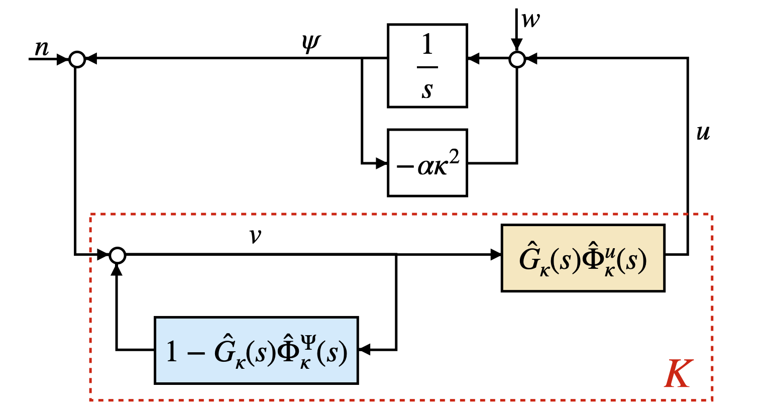
defines an internally stable implementation of the controller in the sense that the closed loop transfer matrices from the exogenous inputs (n^κ​(s),w^κ​(s))(\hat{n}_{\kappa}(s),\hat{w}_{\kappa}(s)) to the internal signals (ψ^κ​(s),u^κ​(s),v^κ​(s))(\hat{\psi}_{\kappa}(s),\hat{u}_{\kappa}(s),\hat{v}_{\kappa}(s)) belong to ℋ∞\mathcal{H}_{\infty}. This implementation is depicted in Figure 1. The input-output map (transfer function) corresponding to (32) is

𝐔=ℱ−1​MK^​(s)​ℱ​𝚿,K^κ​(s)=Φ^κu​(s)Φ^κψ​(s).{\bf U}=\mathcal{F}^{-1}M_{\hat{K}(s)}\mathcal{F}{{\boldsymbol{\Psi}}},~~\hat{K}_{\kappa}(s)=\tfrac{\hat{\Phi}^{u}_{\kappa}(s)}{\hat{\Phi}^{\psi}_{\kappa}(s)}. (33)
Proof:

See Appendix -D. ∎

Remark 2

In the finite-dimensional, discrete-time setting, the analogy of the system GG in (32) is simply the one-time-step delay operator. More care must be taken to select this system in the infinite-dimensional setting due to the potential unboundedness of the operator AA. In this case, the closed-loop map from additive noise to the state to the internal control signal vv is given by (s​I−A)​G−1​(s)(sI-A)G^{-1}(s) (see (36)), which may also be unbounded unless GG is carefully selected.

Refer to caption
Figure 1: Block diagram of the dynamic controller implementation (32) with noisy measurements and exogenous disturbance: ww is additive noise to the state ψ\psi, and ww is additive noise to the control signal uu.

We examine the structure of the controller implementation (32) that results from the optimal solution (31). We select G​(s)=ℱ−1​MG^​(s)​ℱG(s)=\mathcal{F}^{-1}M_{\hat{G}(s)}\mathcal{F} where

G^κ​(s)=s+1+κ2,\displaystyle\hat{G}_{\kappa}(s)=s+1+\kappa^{2}, (34)

to satisfy all conditions of Lemma 3. Note that this is one suitable choice of GG, but it is not obvious how to “best” select GG in general. Then, (32) is specified at frequency κ\kappa as

v^​(s,κ)\displaystyle\hat{v}(s,\kappa) =ψ^​(s,κ)+(1−G^κ​(s)​1s+γ2+α2​κ4)​v^​(s,κ)\displaystyle=\hat{\psi}(s,\kappa)+\left(1-\hat{G}_{\kappa}(s)\tfrac{1}{s+\sqrt{\gamma^{2}+\alpha^{2}\kappa^{4}}}\right)\hat{v}(s,\kappa) (35)
u^​(s,κ)\displaystyle\hat{u}(s,\kappa) =G^κ​(s)​α​κ2−γ2+α2​κ4s+γ2+α2​κ4​v^​(s,κ),\displaystyle=\hat{G}_{\kappa}(s)\tfrac{\alpha\kappa^{2}-\sqrt{\gamma^{2}+\alpha^{2}\kappa^{4}}}{s+\sqrt{\gamma^{2}+\alpha^{2}\kappa^{4}}}\hat{v}(s,\kappa),

where G^\hat{G} is defined in (34). We note that the system ℱ​(I−G​(s)​Φψ​(s))​ℱ−1\mathcal{F}(I-G(s)\Phi^{\psi}(s))\mathcal{F}^{-1} with symbol (1−G^κ​(s)​1s+γ2+α2​κ4)\left(1-\hat{G}_{\kappa}(s)\tfrac{1}{s+\sqrt{\gamma^{2}+\alpha^{2}\kappa^{4}}}\right) is strictly proper, so that the feedback loop in the control implementation in Fig. 1 is well-defined. Using the affine identity in (27) together with routine calculations yields the following closed-loop transfer matrices from (n^κ​(s),w^κ​(s))(\hat{n}_{\kappa}(s),\hat{w}_{\kappa}(s)) to (ψ^κ​(s),u^κ​(s),v^κ​(s))(\hat{\psi}_{\kappa}(s),\hat{u}_{\kappa}(s),\hat{v}_{\kappa}(s)) in the controller implementation:

[ψ^κu^κv^κ]=[Φ^κu​(s)Φ^κψ​(s)(s+α​κ2)​Φ^κu​(s)Φ^κu​(s)(s+α​κ2)​G^κ−1​(s)G^κ−1​(s)]​[n^κw^κ],\displaystyle\begin{bmatrix}\hat{\psi}_{\kappa}\\ \hat{u}_{\kappa}\\ \hat{v}_{\kappa}\end{bmatrix}=\begin{bmatrix}\hat{\Phi}^{u}_{\kappa}(s)&\hat{\Phi}^{\psi}_{\kappa}(s)\\ (s+\alpha\kappa^{2})\hat{\Phi}^{u}_{\kappa}(s)&\hat{\Phi}^{u}_{\kappa}(s)\\ (s+\alpha\kappa^{2})\hat{G}^{-1}_{\kappa}(s)&\hat{G}^{-1}_{\kappa}(s)\end{bmatrix}\begin{bmatrix}\hat{n}_{\kappa}\\ \hat{w}_{\kappa}\\ \end{bmatrix}, (36)

each of which is verified to be the symbol of a multiplication operator in ℋ∞\mathcal{H}_{\infty} for our selected G^.\hat{G}. We numerically compute the spatio-temporal impulse responses (Green’s functions) of the blocks in Fig. 1 and plot their dynamic and static components over the spatial domain for various selections of time in Fig. 2. We note that the kernels of the dynamic components are “more localized” for smaller time values and appear to spread out spatially as time increases.

Refer to caption
Figure 2: Spatio-temporal convolution kernels corresponding to the transfer functions in Fig. 1. Plot (a) shows the yellow block’s static, hΦu​(ξ)h_{\Phi^{u}}(\xi), and dynamic fΦu​(t,ξ)f_{\Phi^{u}}(t,\xi) kernels. Plot (b) shows the blue block’s dynamic kernel fΦψ​(t,ξ)f_{\Phi^{\psi}}(t,\xi).

VI Equivalence to LQR Control

We demonstrate that the solution to our closed-loop ℋ2\mathcal{H}_{2} design problem (LABEL:eq:CL_formulation) recovers the solution to the standard infinite-horizon LQR problem for the diffusion equation.

Proposition 2

The standard LQR problem (LABEL:eq:LQR) and the ℋ2\mathcal{H}_{2} problem of interest (LABEL:eq:CL_formulation) have the same solution KoptK^{\rm opt}.

Proof:

First, we compute the solution to the LQR formulation (LABEL:eq:LQR) using standard approaches [2, 7]. We solve the operator-valued Riccati equation

⟨A​η,F​ϑ⟩L2​(𝕋)+⟨F​η,A​ϑ⟩L2​(𝕋)+γ2​⟨η,ϑ⟩L2​(𝕋)\displaystyle\left<A\eta,F\vartheta\right>_{L^{2}(\mathbb{T})}+\left<F\eta,A\vartheta\right>_{L^{2}(\mathbb{T})}+\gamma^{2}\left<\eta,\vartheta\right>_{L^{2}(\mathbb{T})} (37)
=⟨F​η,F​ϑ⟩L2​(𝕋).\displaystyle=\left<F\eta,F\vartheta\right>_{L^{2}(\mathbb{T})}.

The solution FF to (37) is known to be spatially-invariant [2], and the symbol of ℱ​F​ℱ−1=MF^\mathcal{F}F\mathcal{F}^{-1}=M_{\hat{F}} can be obtained by solving the family of scalar-valued algebraic Riccati equations (AREs) parameterized by κ∈ℤ:\kappa\in\mathbb{Z}:

−α​κ2​F^κ−F^κ​α​κ2−F^κ2+γ2=0.-\alpha\kappa^{2}\hat{F}_{\kappa}-\hat{F}_{\kappa}\alpha\kappa^{2}-\hat{F}_{\kappa}^{2}+\gamma^{2}=0. (38)

The unique solution F^κ>0\hat{F}_{\kappa}>0 to (38) is F^κ=−α​κ2+α2​κ4+γ2,\hat{F}_{\kappa}=-\alpha\kappa^{2}+\sqrt{\alpha^{2}\kappa^{4}+\gamma^{2}}, and the optimal state feedback gain is thus given by KLQR=ℱ​MK^LQR​ℱ−1K^{\rm LQR}=\mathcal{F}M_{\hat{K}^{\rm LQR}}\mathcal{F}^{-1} where

K^κLQR=−F^κ=α​κ2−α2​κ4+γ2.\hat{K}^{\rm LQR}_{\kappa}=-\hat{F}_{\kappa}=\alpha\kappa^{2}-\sqrt{\alpha^{2}\kappa^{4}+\gamma^{2}}. (39)

We next obtain the input-output mapping specified by the controller implementation (35) using (33) as

K^κℋ2​(s)=Φ^κu​(s)Φ^κψ​(s)=α​κ2−γ2+α2​κ4.\hat{K}^{\mathcal{H}_{2}}_{\kappa}(s)=\frac{\hat{\Phi}^{u}_{\kappa}(s)}{\hat{\Phi}^{\psi}_{\kappa}(s)}=\alpha\kappa^{2}-\sqrt{\gamma^{2}+\alpha^{2}\kappa^{4}}. (40)

This is indeed equal to the static state feedback gain K^L​Q​R\hat{K}^{LQR}, thus KLQR=Kℋ2=Kopt.K^{\rm LQR}=K^{\mathcal{H}_{2}}=K^{\rm opt}. ∎

We know that KoptK^{\rm opt} will be a spatial convolution operator

u​(t,θ)=∫ξ∈𝕋k​(θ−ξ)​ψ​(t,ξ)​𝑑t,u(t,\theta)=\int_{\xi\in\mathbb{T}}k(\theta-\xi)\psi(t,\xi)dt, (41)

where k​(θ)=(ℱ−1​K^)​(θ).k(\theta)=(\mathcal{F}^{-1}\hat{K})(\theta). Numerical integration shows that k​(θ)k(\theta) exhibits spatial decay away from the origin (see Fig. 2).

We compare the static controller KoptK^{\rm opt} to the dynamic controller implementation (35) depicted in Fig. 1. As previously noted, the transfer function (I−G​(s)​Φψ​(s))\left(I-G(s){\Phi}^{\psi}(s)\right) is strictly proper, thus its corresponding convolution kernel has only a dynamic part, which we denote as fΦψ​(t,θ)f_{\Phi^{\psi}}(t,\theta). The transfer function G​(s)​Φu​(s)G(s)\Phi^{u}(s) has a corresponding convolution kernel with both a static and dynamic part, which we denote as hΦu​(θ),fΦu​(t,θ)h_{\Phi^{u}}(\theta),f_{\Phi^{u}}(t,\theta), respectively. The static (direct feedthrough) component of G​(s)​Φu​(s)G(s)\Phi^{u}(s) is obtained by evaluating its Fourier symbol in the limit as s→∞s\to\infty,

ℱ−1​lims→∞G^​(s,κ)​Φ^u​(s,κ)=hΦu​(θ)=(ℱ−1​K^opt)​(θ),\mathcal{F}^{-1}\lim_{s\to\infty}\hat{G}(s,\kappa)\hat{\Phi}^{u}(s,\kappa)=h_{\Phi^{u}}(\theta)=(\mathcal{F}^{-1}\hat{K}^{\rm opt})(\theta),

which shows that the static part of the implementation (35) recovers the static LQR gain, as expected. The “dynamic components” of the systems G​(s)​Φu​(s)G(s)\Phi^{u}(s) and (I−G​(s)​Φψ​(s))\left(I-G(s){\Phi}^{\psi}(s)\right) cancel each other out, leaving only the static feedback policy Kopt.K^{\rm opt}. This is confirmed in the plot of hΦu​(θ),fΦu​(t,θ),fΦψ​(t,θ)h_{\Phi^{u}}(\theta),f_{\Phi^{u}}(t,\theta),f_{\Phi^{\psi}}(t,\theta) shown in Fig. 2.

VII Incorporation of Spatio-Temporal Decay Rate Constraints

Without constraints, the closed-loop formulation of the ℋ2\mathcal{H}_{2} problem (LABEL:eq:CL_formulation) is equivalent to a standard LQR problem. The advantage of this closed-loop formulation is that it remains convex when spatio-temporal constraints are incorporated. A similar problem has been studied in [3], where necessary and sufficient conditions for convexity were dependent on “funnel causality” properties of the underlying system and desired constraint. Notably, our formulation does not rely on these conditions and thus admits a broader range of constraints while preserving convexity.

An added constraint that I−G​Φψ,G​Φu∈𝒮I-G\Phi^{\psi},G\Phi^{u}\in\mathcal{S} enforces a structural constraint on the components of our controller. In this case, formulation (LABEL:eq:CL_formulation) becomes:

arg​minΦψ,Φu∈H∞⁡‖C​Φψ+D​Φu‖ℋ2\displaystyle\operatorname*{arg\,min}_{\Phi^{\psi},\Phi^{u}\in H_{\infty}}~\left\|C\Phi^{\psi}+D\Phi^{u}\right\|_{\mathcal{H}_{2}} (42)
s.t.Φψ,Φu spatially invariant\displaystyle~~~~~{\rm s.t.}~~~~~~\Phi^{\psi},\Phi^{u}\text{ spatially invariant}
Φψ,Φu​ satisfy (LABEL:eq:affine_innerProduct),\displaystyle~~~~~~~~~~~~~~~\Phi^{\psi},\Phi^{u}\text{ satisfy \eqref{eq:affine_innerProduct}},
I−G​Φψ,G​Φu∈𝒮.\displaystyle~~~~~~~~~~~~~~~~I-G\Phi^{\psi},G\Phi^{u}\in\mathcal{S}.

So long as the set 𝒮\mathcal{S} defines a convex constraint on Φu,Φψ\Phi^{u},\Phi^{\psi} the constrained problem (LABEL:eq:constrained) will be convex.

Of particular interest are constraints that specify a degree of spatio-temporal locality on Φψ\Phi^{\psi} and Φu\Phi^{u}. In the finite-dimensional, discrete-time, finite-horizon setting, such constraints take the form of spatio-temporal FIR constraints on the closed-loop system [22]. In the continuous spatial and temporal domain setting, we believe it is more natural to impose a level of decay, or “approximate locality”. This choice might be viewed as analogue to the “leaky” SLS problem presented in [15].

One possible spatio-temporal constraint is when 𝒮\mathcal{S} is the set of linear PDEs whose Green’s functions ρ​(⋅,⋅)\rho(\cdot,\cdot) satisfy

‖ρ​(⋅,t)−ρT​(⋅,t)‖L2​(𝕋)<ϵ​(t)\|\rho(\cdot,t)-\rho_{T}(\cdot,t)\|_{L_{2}(\mathbb{T})}<\epsilon(t) (43)

where ρT\rho_{T} is the spatial truncation of ρ\rho given by

ρT​(θ,⋅)={ρ​(θ,⋅)|θ|<r0otherwise\rho_{T}(\theta,\cdot)=\begin{cases}\rho(\theta,\cdot)&|\theta|<r\\ 0&{\rm otherwise}\end{cases}

and r≤πr\leq\pi is the truncation radius that encodes communication limitations. This constraint ensures that the ‘tails’ of ρ\rho are sufficiently small, potentially enforcing spatial locality. Choosing ϵ​(t)\epsilon(t) to grow in tt allows ρ\rho to be less localized in space as time increases. While constraining ρ\rho to have compact support as in [5] admits desirable computational properties, the decay constraint (43) is perhaps more physically relevant. This set 𝒮\mathcal{S} is convex, and guarantees that a spatially truncated version of controller will perform well using small gain arguments.

Obtaining analytical and numerical solutions to constrained problems of the form (LABEL:eq:constrained) is the subject of ongoing work. While analytical solutions will require clever formulations of the constraints, numerical solutions may leverage approaches such as those presented in [6] and benefit from computational approaches like [20].

VIII Conclusion

It was shown that the infinite-horizon LQR problem for the diffusion equation over the unit circle can be reformulated as an ℋ2\mathcal{H}_{2} problem over the system’s closed-loop responses, analogous to the finite-dimensional System Level Synthesis methodology. An implementation of this optimal controller built from these closed-loop responses was shown to preserve internal stability. It was further illustrated that this closed-loop formulation admits a class of spatio-temporal constraints on the closed-loop responses while preserving convexity. Generalizations of this work to general linear distributed parameter systems are the subject of ongoing work. Of particular interest include incorporation of boundary conditions through an embedding approach [9] or alternate representations [17]; and comparison of analytical results from this work to the computational approach of [6].

References

  • [1] J. Anderson, J. C. Doyle, S. H. Low, and N. Matni (2019) System level synthesis. Annual Reviews in Control 47, pp. 364–393. Cited by: §I.
  • [2] B. Bamieh, F. Paganini, and M.A. Dahleh (2002) Distributed control of spatially invariant systems. IEEE Transactions on Automatic Control 47 (7), pp. 1091–1107. External Links: Document Cited by: §-B, §III-A, §VI, §VI.
  • [3] B. Bamieh and P. G. Voulgaris (2005) A convex characterization of distributed control problems in spatially invariant systems with communication constraints. Systems & control letters 54 (6), pp. 575–583. Cited by: §I, §VII.
  • [4] H. Banks and K. Kunisch (1984) The linear regulator problem for parabolic systems. SIAM Journal on Control and Optimization 22 (5), pp. 684–698. Cited by: §III-B.
  • [5] L. Conger, A. P. Leeman, and F. Hoffmann (2024) Convex constrained controller synthesis for evolution equations. arXiv preprint arXiv:2410.02658. Cited by: §VII.
  • [6] L. Conger, A. P. Leeman, and F. Hoffmann (2025) Convex constrained controller synthesis for evolution equations. In 2025 American Control Conference (ACC), pp. 1169–1176. Cited by: §I, §I, §I, §VII, §VIII.
  • [7] R. Curtain and H. Zwart (2020) Introduction to infinite-dimensional systems theory: a state-space approach. Vol. 71, Springer Nature. Cited by: §III-B, §III, §IV-A, §IV-A, §IV-A, §IV-A, §VI, Definition 1.
  • [8] G. E. Dullerud and F. Paganini (2013) A course in robust control theory: a convex approach. Vol. 36, Springer Science & Business Media. Cited by: §IV-C.
  • [9] J. P. Epperlein and B. Bamieh (2016) Spatially invariant embeddings of systems with boundaries. In 2016 American Control Conference (ACC), pp. 6133–6139. Cited by: §VIII.
  • [10] J. Gibson and A. Adamian (1991) Approximation theory for linear-quadratic-Gaussian control of flexible structures. SIAM journal on control and optimization 29 (1), pp. 1–37. Cited by: §I.
  • [11] E. Jensen and B. Bamieh (2018) Optimal spatially-invariant controllers with locality constraints: a system level approach. In 2018 Annual American Control Conference (ACC), pp. 2053–2058. Cited by: §I.
  • [12] E. Jensen and B. Bamieh (2021) An explicit parametrization of closed loops for spatially distributed controllers with sparsity constraints. IEEE Transactions on Automatic Control 67 (8), pp. 3790–3805. Cited by: §I.
  • [13] I. Jung, Z. Peng, and Y. Rahmat-Samii (2024) Recent advances in reconfigurable electromagnetic surfaces: engineering design, full-wave analysis, and large-scale optimization. Electromagnetic Science 2 (3), pp. 1–25. Cited by: §I.
  • [14] V. Kučera (2006) The H2 control problem: state-space and transfer-function solutions. In 2006 14th Mediterranean Conference on Control and Automation, pp. 1–5. Cited by: §-A.
  • [15] N. Matni, Y. Wang, and J. Anderson (2017) Scalable system level synthesis for virtually localizable systems. In 2017 IEEE 56th Annual Conference on Decision and Control (CDC), pp. 3473–3480. Cited by: §VII.
  • [16] K. A. Morris (2020) Controller design for distributed parameter systems. Springer. Cited by: §-B, §I, §III, footnote 1.
  • [17] M. M. Peet (2021) A partial integral equation (PIE) representation of coupled linear PDEs and scalable stability analysis using LMIs. Automatica 125, pp. 109473. Cited by: §VIII.
  • [18] M. Rotkowitz and S. Lall (2005) A characterization of convex problems in decentralized control. IEEE transactions on Automatic Control 50 (12), pp. 1984–1996. Cited by: §I.
  • [19] Ş. Sabău, A. Sperilă, C. Oară, and A. Jadbabaie (2023) Network realization functions for optimal distributed control. IEEE Transactions on Automatic Control 68 (12), pp. 8059–8066. Cited by: §I.
  • [20] S. Shivakumar, A. Das, and M. M. Peet (2020) PIETOOLS: a MATLAB toolbox for manipulation and optimization of partial integral operators. In 2020 American Control Conference (ACC), pp. 2667–2672. Cited by: §VII.
  • [21] M. Wang, L. Liang, W. Cheng, W. Zhang, R. Chen, and H. Zhang (2024) Reconfigurable-intelligent-surface assisted orbital-angular-momentum secure communications. IEEE Transactions on Vehicular Technology 73 (11), pp. 17788–17793. External Links: Document Cited by: §I.
  • [22] Y. Wang, N. Matni, and J. C. Doyle (2019) A system-level approach to controller synthesis. IEEE Transactions on Automatic Control 64 (10), pp. 4079–4093. Cited by: §I, §I, §IV-B, §VII.
  • [23] Y. Yang, J. Seong, M. Choi, J. Park, G. Kim, H. Kim, J. Jeong, C. Jung, J. Kim, G. Jeon, K. Lee, D. H. Yoon, and J. Rho (2023) Integrated metasurfaces for re-envisioning a near-future disruptive optical platform. Light: Science & Applications 12 (1), pp. 152. Cited by: §I.
  • [24] Y. Zheng, L. Furieri, A. Papachristodoulou, N. Li, and M. Kamgarpour (2020) On the equivalence of Youla, system-level, and input–output parameterizations. IEEE Transactions on Automatic Control 66 (1), pp. 413–420. Cited by: §I.

-A Proof of Proposition 1

Proof:

We replace the implicit constraint (30f) with an analogous explicit constraint using the following Lemma:

Lemma 4

Fix κ∈ℤ.\kappa\in\mathbb{Z}. The single-input single-output (SISO) transfer functions Φ^κψ,Φ^κu\hat{\Phi}^{\psi}_{\kappa},~\hat{\Phi}^{u}_{\kappa} satisfy Φ^κψ,Φ^κu∈ℛ​ℋ2\hat{\Phi}^{\psi}_{\kappa},~\hat{\Phi}^{u}_{\kappa}\in\mathcal{RH}_{2} and (30f) if and only if they are of the form

Φ^κψ​(s)\displaystyle\hat{\Phi}^{\psi}_{\kappa}(s) =1s+1​(1+ρ^κ​(s)),\displaystyle=\frac{1}{s+1}\left(1+\hat{\rho}_{\kappa}(s)\right), (44)
Φ^κu​(s)\displaystyle\hat{\Phi}^{u}_{\kappa}(s) =α​κ2−1s+1+s+α​κ2s+1​ρ^κ​(s)\displaystyle=\frac{\alpha\kappa^{2}-1}{s+1}+\frac{s+\alpha\kappa^{2}}{s+1}\hat{\rho}_{\kappa}(s)

for some SISO transfer function ρ^κ​(s)∈ℛ​ℋ2.\hat{\rho}_{\kappa}(s)\in\mathcal{RH}_{2}.

Proof:

It is simple to verify sufficiency, so we only prove necessity. We write (30f) as

Φ^κu​(s)=((s+1)−(−α​κ2+1))​Φ^κψ​(s)−1.\hat{\Phi}_{\kappa}^{u}(s)=\left((s+1)-(-\alpha\kappa^{2}+1)\right)\hat{\Phi}_{\kappa}^{\psi}(s)-1. (45)

Since Φ^κψ​(s)∈ℛ​ℋ2,\hat{\Phi}_{\kappa}^{\psi}(s)\in\mathcal{RH}_{2}, it follows that Φ^κu​(s)∈ℛ​ℋ2\hat{\Phi}_{\kappa}^{u}(s)\in\mathcal{RH}_{2} only if lims→∞(s+1)​Φ^κψ​(s)=1.\lim_{s\to\infty}(s+1)\hat{\Phi}_{\kappa}^{\psi}(s)=1. This means Φ^κψ​(s)\hat{\Phi}_{\kappa}^{\psi}(s) is of the form Φ^κψ​(s)=1s+1​(1+ρ^κ​(s))\hat{\Phi}_{\kappa}^{\psi}(s)=\frac{1}{s+1}(1+\hat{\rho}_{\kappa}(s)) for some ρ^κ​(s)∈ℛ​ℋ2.\hat{\rho}_{\kappa}(s)\in\mathcal{RH}_{2}. Plugging this into (45) gives the explicit formulas (44). ∎

We can now use the parameterization (44) to write (30) as an unconstrained ℋ2\mathcal{H}_{2} design problem over a single SISO transfer function decision variable ρ^κ:\hat{\rho}_{\kappa}:

arg​minρ^κ∈ℛ​ℋ2⁡‖[γs+1α​κ2−1s+1]+[γs+1α​κ2+ss+1]​ρ^κ⏟G​(ρ^κ):=H+N​ρ^κ‖ℋ22\operatorname*{arg\,min}_{\hat{\rho}_{\kappa}\in\mathcal{RH}_{2}}\Bigg\|\underbrace{\begin{bmatrix}\frac{\gamma}{s+1}\\ \frac{\alpha\kappa^{2}-1}{s+1}\end{bmatrix}+\begin{bmatrix}\frac{\gamma}{s+1}\\ \frac{\alpha\kappa^{2}+s}{s+1}\end{bmatrix}\hat{\rho}_{\kappa}}_{G(\hat{\rho}_{\kappa}):=H+N\hat{\rho}_{\kappa}}\Bigg\|^{2}_{\mathcal{H}_{2}} (46)

where H∈ℛℋ2,N=∈ℛℋ∞H\in\mathcal{RH}_{2},N=\in\mathcal{RH}_{\infty}. We want to leverage the following result [14]:

Lemma 5

Let E∈ℛ​ℋ2,F∈ℛ​ℋ∞E\in\mathcal{RH}_{2},F\in\mathcal{RH}_{\infty} with FF inner and F∼​E∈ℛ​ℋ2⟂.F^{\sim}E\in\mathcal{RH}_{2}^{\perp}. Then ∀T∈ℛ​ℋ2,\forall T\in\mathcal{RH}_{2},

‖E−F​T‖ℋ22=‖E‖ℋ22+‖T‖ℋ22.\|E-FT\|^{2}_{\mathcal{H}_{2}}=\|E\|^{2}_{\mathcal{H}_{2}}+\|T\|^{2}_{\mathcal{H}_{2}}.

Let N=Ui​UoN=U_{i}U_{o} be the inner-outer factorization of NN where

Ui=[γs+γ2+α2​κ4s+α​κ2s+γ2+α2​κ4],U0=s+γ2+α2​κ4s+1U_{i}=\begin{bmatrix}\frac{\gamma}{s+\sqrt{\gamma^{2}+\alpha^{2}\kappa^{4}}}\\ \frac{s+\alpha\kappa^{2}}{s+\sqrt{\gamma^{2}+\alpha^{2}\kappa^{4}}}\end{bmatrix},~U_{0}=\frac{s+\sqrt{\gamma^{2}+\alpha^{2}\kappa^{4}}}{s+1} (47)

so that Ui,Uo∈ℛ​ℋ∞U_{i},U_{o}\in\mathcal{RH}_{\infty} and G​(ρ^κ)=H+Ui​Uo​ρ^κ.G(\hat{\rho}_{\kappa})=H+U_{i}U_{o}\hat{\rho}_{\kappa}. Then Ui∼​G​(ρ^κ)=Ui∼​H+Uo​ρ^κ=Y+Y⟂+UoU_{i}^{\sim}G(\hat{\rho}_{\kappa})=U_{i}^{\sim}H+U_{o}\hat{\rho}_{\kappa}=Y+Y^{\perp}+U_{o} where Y,Y⟂Y,Y^{\perp} are the projections of Ui∼U_{i}^{\sim} onto ℛ​ℋ2,ℛ​ℋ2⟂,\mathcal{RH}_{2},\mathcal{RH}_{2}^{\perp}, respectively. This gives Uo​ρ^κ=Ui∼​G​(ρ^κ)−Y−Y⟂U_{o}\hat{\rho}_{\kappa}=U_{i}^{\sim}G(\hat{\rho}_{\kappa})-Y-Y^{\perp} so that

G​(ρ^κ)\displaystyle G(\hat{\rho}_{\kappa}) =(H−Ui​Y)⏟=⁣:G1−Ui​(Y⟂−Ui∼​G​(ρ^κ))⏟=⁣:N1.\displaystyle=\underbrace{(H-U_{i}Y)}_{=:G_{1}}-U_{i}\underbrace{(Y^{\perp}-U_{i}^{\sim}G(\hat{\rho}_{\kappa}))}_{=:N_{1}}. (48)

Note that G1∈ℛ​ℋ2G_{1}\in\mathcal{RH}_{2}, N1=−Y−Uo​ρ^κ∈ℛ​ℋ2N_{1}=-Y-U_{o}\hat{\rho}_{\kappa}\in\mathcal{RH}_{2}, and Ui∼​G1=Ui∼​H−Y=Y⟂∈ℛ​ℋ2⟂U_{i}^{\sim}G_{1}=U_{i}^{\sim}H-Y=Y^{\perp}\in\mathcal{RH}_{2}^{\perp} so that by Lemma 5,

arg​minρ^κ∈ℛ​ℋ2⁡‖G​(ρ^κ)‖ℋ22=arg​minρ^κ∈ℛ​ℋ2⁡‖G1−Ui​N1‖ℋ22\displaystyle\operatorname*{arg\,min}_{\hat{\rho}_{\kappa}\in\mathcal{RH}_{2}}\|G(\hat{\rho}_{\kappa})\|^{2}_{\mathcal{H}_{2}}=\operatorname*{arg\,min}_{\hat{\rho}_{\kappa}\in\mathcal{RH}_{2}}\|G_{1}-U_{i}N_{1}\|^{2}_{\mathcal{H}_{2}} (49)
=arg​minρ^κ∈ℛ​ℋ2⁡‖G1‖ℋ22+‖N1‖ℋ22=arg​minρ^κ∈ℛ​ℋ2⁡‖N1‖ℋ22\displaystyle~~=\operatorname*{arg\,min}_{\hat{\rho}_{\kappa}\in\mathcal{RH}_{2}}\|G_{1}\|^{2}_{\mathcal{H}_{2}}+\|N_{1}\|^{2}_{\mathcal{H}_{2}}=\operatorname*{arg\,min}_{\hat{\rho}_{\kappa}\in\mathcal{RH}_{2}}\|N_{1}\|^{2}_{\mathcal{H}_{2}} (50)

since G1G_{1} does not depend on ρ^κ\hat{\rho}_{\kappa}. To solve we set N1=0N_{1}=0 resulting in ρ^κopt.​(s)=Uo−1​Y=−Uo−1⋅(Ui∼​H)|ℛ​ℋ2\hat{\rho}_{\kappa}^{\rm opt.}(s)=U_{o}^{-1}Y=-U_{o}^{-1}\cdot(U_{i}^{\sim}H)\Big|_{\mathcal{RH}_{2}} so that the solution to (46) is

ρ^κopt.​(s)=1−γ2+α2​κ4s+γ2+α2​κ4,\hat{\rho}_{\kappa}^{\rm opt.}(s)=\frac{1-\sqrt{\gamma^{2}+\alpha^{2}\kappa^{4}}}{s+\sqrt{\gamma^{2}+\alpha^{2}\kappa^{4}}}, (51)

which we plug into (44) to see (31) solves (30). ∎

-B Proof of Lemma 1

Proof:

Spatial invariance of KK implies spatial invariance of Φψ\Phi^{\psi} and Φu\Phi^{u} from the relationship (22) and properties of spatially-invariant systems. Let Σ​(AK,BK,CK,DK)\Sigma(A^{K},B^{K},C^{K},D^{K}) denote the system with operator-valued transfer function KK. lims→∞K​(s)=DK\lim_{s\rightarrow\infty}K(s)=D^{K} so that by equation (22), lims→∞Φψ​(s)=0\lim_{s\rightarrow\infty}\Phi^{\psi}(s)=0 and lims→∞Φu​(s)=0\lim_{s\rightarrow\infty}\Phi^{u}(s)=0. The systems with transfer functions Φψ,Φu\Phi^{\psi},\Phi^{u} and 𝔽​(P;K)\mathbb{F}(P;K) can be represented as linear, spatially-invariant distributed parameter systems Σ​(Ac.l.,I,I,0),\Sigma(A_{\rm c.l.},I,I,0), Σ​(Ac.l.,I,Cu,0),\Sigma(A_{\rm c.l.},I,C_{u},0), and Σ​(Ac.l.,I,Cc.l.,0),\Sigma(A_{\rm c.l.},I,C_{\rm c.l.},0), respectively. Since KK is internally stabilizing, {TAc.l.​(t)}\{T_{A_{\rm c.l.}(t)}\} is an exponentially stable C0C_{0}-semigroup, and thus the transfer function representations of these systems - Φψ,Φu\Phi^{\psi},\Phi^{u} and 𝔽​(P;K)\mathbb{F}(P;K) - are well-defined on {s∈ℂ;Re​(s)≥0}.\{s\in\mathbb{C};~{\rm Re}(s)\geq 0\}. By Plancherel’s Theorem, supRe​(s)≥0‖Φψ​(s)‖L2​(𝕋)→L2​(𝕋)=supRe​(s)≥0‖MΦ^ψ​(s)‖ℓ2​(ℤ)→ℓ2​(ℤ),\sup_{{\rm Re}(s)\geq 0}~\|\Phi^{\psi}(s)\|_{L^{2}(\mathbb{T})\rightarrow L^{2}(\mathbb{T})}=\sup_{{\rm Re}(s)\geq 0}~\|M_{\hat{\Phi}^{\psi}(s)}\|_{\ell^{2}(\mathbb{Z})\rightarrow\ell^{2}(\mathbb{Z})}, and similarly for Φu,\Phi^{u}, so that the pointwise condition (LABEL:eq:Hinf_frequency) is equivalent to (LABEL:eq:Hinf_condition).

To show that (LABEL:eq:Hinf_frequency) holds, note that exponential stability of {TAc.l.​(t)}\{T_{A_{\rm c.l.}}(t)\} is equivalent to exponential stability of the C0C_{0}-semigroup generated by MA^c.l.=ℱ​Ac.l.​ℱ−1M_{\hat{A}_{\rm c.l.}}=\mathcal{F}A_{\rm c.l.}\mathcal{F}^{-1}. This is a semigroup of multiplication operators, whose symbols are of the form et​A^c.l.​(κ),e^{t\hat{A}_{\rm c.l.}(\kappa)}, where A^c.l.​(κ)\hat{A}_{\rm c.l.}(\kappa) is a finite-dimensional matrix for each κ.\kappa. Thus, there exists m,η>0m,\eta>0 for which ‖TMA^c.l.​(t)‖≤m​e−η​t.\|T_{M_{\hat{A}_{\rm c.l.}}}(t)\|\leq me^{-\eta t}. The operator norm of each multiplication operator in this semigroup is given by the ∞\infty-norm of its symbol [2], so that for each t≥0,t\geq 0,

m​e−η​t≥‖TMA^c.l.​(t)‖=supκσmax​{et​A^c.l.​(κ)},me^{-\eta t}\geq\|T_{M_{\hat{A}_{\rm c.l.}}}(t)\|=\sup_{\kappa}\sigma_{\max}\{e^{t\hat{A}_{\rm c.l.}(\kappa)}\}, (52)

where σmax​(N)\sigma_{\max}(N) denotes the maximum singular value of a matrix N.N. In addition to internal stabilization for each fixed κ\kappa, uniform stabilizability [16, Def. 4.9] of the family of systems (A^​(κ),B^​(κ))(\hat{A}(\kappa),\hat{B}(\kappa)) as |κ|→∞|\kappa|\to\infty ensures that the supremum in (52) is finite. Since B^​(κ)​K^​(κ)\hat{B}(\kappa)\hat{K}(\kappa) is uniformly bounded and A^​(κ)=−α​κ2​I\hat{A}(\kappa)=-\alpha\kappa^{2}I, lim|κ|→∞A^c.l.​(κ)→−∞\lim_{|\kappa|\to\infty}\hat{A}_{\rm c.l.}(\kappa)\to-\infty, so (A^​(κ),B^​(κ))(\hat{A}(\kappa),\hat{B}(\kappa)) is uniformly stabilizable. For each fixed κ,\kappa, the H∞H_{\infty} norm of the finite-dimensional transfer matrix Φ^κψ​(s)=(s​I−A^c.l.​(κ))−1\hat{\Phi}^{\psi}_{\kappa}(s)=(sI-\hat{A}_{\rm c.l.}(\kappa))^{-1}, given by supRe​(s)≥0σmax​{(s​I−A^c.l.​(κ))−1},\sup_{{\rm Re}(s)\geq 0}\sigma_{\rm max}\{(sI-\hat{A}_{\rm c.l.}(\kappa))^{-1}\}, is equal to the operator norm of 𝒪∈ℒ​(L2​[0,∞))\mathcal{O}\in\mathcal{L}(L^{2}[0,\infty)) defined by (𝒪​f)​(t)=∫0te(t−τ)​A^c.l.​(κ)​f​(τ)​𝑑τ.(\mathcal{O}f)(t)=\int_{0}^{t}e^{(t-\tau)\hat{A}_{\rm c.l.}(\kappa)}f(\tau)d\tau. By (52),

‖(𝒪​f)​(t)‖=‖∫0te(t−τ)​A^c.l.​(κ)​f​(τ)​𝑑τ‖\displaystyle\|(\mathcal{O}f)(t)\|=\left\|\int_{0}^{t}e^{(t-\tau)\hat{A}_{\rm c.l.}(\kappa)}f(\tau)d\tau\right\| (53)
=‖et​A^c.l.​(κ)​∫0te−τ​A^c.l.​(κ)​f​(τ)​𝑑τ‖\displaystyle=\left\|e^{t\hat{A}_{\rm c.l.}(\kappa)}\int_{0}^{t}e^{-\tau\hat{A}_{\rm c.l.}(\kappa)}f(\tau)d\tau\right\|
≤‖et​A^c.l.​(κ)‖⋅sup0≤τ≤t‖e−τ​A^c.l.​(κ)‖⋅‖f‖\displaystyle\leq\|e^{t\hat{A}_{\rm c.l.}(\kappa)}\|\cdot\sup_{0\leq\tau\leq t}\|e^{-\tau\hat{A}_{\rm c.l.}(\kappa)}\|\cdot\|f\|
=‖et​A^c.l.​(κ)‖⋅‖f‖≤m​e−η​t​‖f‖,\displaystyle=\|e^{t\hat{A}_{\rm c.l.}(\kappa)}\|\cdot\|f\|~\leq me^{-\eta t}\|f\|,

where each ∥⋅∥\|\cdot\| in (LABEL:eq:app_computations) is the L2​[0,∞)L^{2}[0,\infty) norm. Then, ‖𝒪​f‖≤‖f‖​∫0∞(m​e−η​t)2​𝑑t,\|\mathcal{O}f\|\leq\|f\|\int_{0}^{\infty}(me^{-\eta t})^{2}dt, so that the operator norm of 𝒪∈ℒ​(L2​[0,∞))\mathcal{O}\in\mathcal{L}(L^{2}[0,\infty)) is upper bounded by m2η<∞\tfrac{m^{2}}{\eta}<\infty, independent of κ.\kappa. Thus, supκ∈ℤsupRe​(s)≥0Φ^κψ​(s)≤m2η<∞,\sup_{\kappa\in\mathbb{Z}}\sup_{{\rm Re}(s)\geq 0}\hat{\Phi}^{\psi}_{\kappa}(s)\leq\tfrac{m^{2}}{\eta}<\infty, verifying the first inequality in (LABEL:eq:Hinf_frequency). Next, by definition of C,DC,D and the relationship (23), we have that 𝔽​(P;K)​(κ,s)=[γ​Φκψ​(s)0]+[01]​Φκu​(s)\mathbb{F}(P;K)(\kappa,s)=\begin{bmatrix}\gamma\Phi^{\psi}_{\kappa}(s)\\ 0\end{bmatrix}+\begin{bmatrix}0\\ 1\end{bmatrix}\Phi^{u}_{\kappa}(s), so that

supRe​(s)≥0supκ∈ℤ|Φ^κu​(s)|≤‖𝔽​(P;K)−γ​[Φψ0]‖ℋ2\displaystyle\sup_{{\rm Re}(s)\geq 0}\sup_{\kappa\in\mathbb{Z}}\big|\hat{\Phi}^{u}_{\kappa}(s)\big|\leq\left\|\mathbb{F}(P;K)-\gamma\begin{bmatrix}\Phi^{\psi}\\ 0\end{bmatrix}\right\|_{\mathcal{H}_{2}}
≤‖𝔽​(P;K)‖ℋ2+γ​supRe​(s)≥0,κ∈ℤ|Φ^κψ​(s)|<∞,\displaystyle~~~~~\leq~\left\|\mathbb{F}(P;K)\right\|_{\mathcal{H}_{2}}+\gamma\sup_{{\rm Re}(s)\geq 0,\kappa\in\mathbb{Z}}\big|\hat{\Phi}^{\psi}_{\kappa}(s)\big|<\infty,

verifying the second inequality in (LABEL:eq:Hinf_frequency).∎

-C Proof of Lemma 2

Proof:

First, we demonstrate the equivalence of (LABEL:eq:affine_innerProduct) to (27) for each s∈{s∈ℂ;Re​(s)≥0}s\in\{s\in\mathbb{C};~{\rm Re}(s)\geq 0\}. By Plancherel’s Theorem, for a fixed s,s, (LABEL:eq:affine_innerProduct) is equivalent to ¡^η, M_^Ω(s) ^ϑ ¿_ℓ^2(Z) - ¡ ^η, M_^Φ^u(s) ^ϑ ¿_ℓ^2(Z) = ¡ ^η, ^ϑ ¿_ℓ^2(Z), for all η^,ϑ^∈ℓ2​(ℤ),\hat{\eta},\hat{\vartheta}\in\ell^{2}(\mathbb{Z}), where Ω^κ​(s)=((s+1)−(A^κ+1))​Φ^κψ​(s)\hat{\Omega}_{\kappa}(s)=\left((s+1)-(\hat{A}_{\kappa}+1)\right)\hat{\Phi}^{\psi}_{\kappa}(s). Expanding these inner products over ℓ2​(ℤ)\ell^{2}(\mathbb{Z}) gives 0=∑κ∈ℤη^κ​(Ω^κ​(s)−Φ^κu−1)​ϑ^κ.0=\sum_{\kappa\in\mathbb{Z}}\hat{\eta}_{\kappa}\left(\hat{\Omega}_{\kappa}(s)-\hat{\Phi}^{u}_{\kappa}-1\right)\hat{\vartheta}_{\kappa}. As this sum holds for all η^,ϑ^∈ℓ2​(ℤ),\hat{\eta},\hat{\vartheta}\in\ell^{2}(\mathbb{Z}), we have that 0=Ω^κ​(s)−Φ^κu−1,0=\hat{\Omega}_{\kappa}(s)-\hat{\Phi}^{u}_{\kappa}-1, for all κ∈ℤ\kappa\in\mathbb{Z} or equivalently ((s+1)−(−α​κ2+1))​Φ^κψ​(s)−Φ^κu​(s)=1\left((s+1)-(-\alpha\kappa^{2}+1)\right)\hat{\Phi}^{\psi}_{\kappa}(s)-\hat{\Phi}_{\kappa}^{u}(s)=1 for all κ∈ℤ\kappa\in\mathbb{Z}. Next, we demonstrate that the pointwise condition (27) holds. From (22), we have that

Φ^κψ​(s)=1s−A^κ−K^κ​(s)=1(s+1)−(−α​κ2+1)−K^κ​(s),\displaystyle\hat{\Phi}^{\psi}_{\kappa}(s)=\tfrac{1}{s-\hat{A}_{\kappa}-\hat{K}_{\kappa}(s)}=\tfrac{1}{(s+1)-(-\alpha\kappa^{2}+1)-\hat{K}_{\kappa}(s)}, (54)
Φ^κψ​(s)=K^κ​(s)s−A^κ−K^κ​(s)=K^κ​(s)(s+1)−(−α​κ2+1)−K^κ​(s),\displaystyle\hat{\Phi}^{\psi}_{\kappa}(s)=\tfrac{\hat{K}_{\kappa}(s)}{s-\hat{A}_{\kappa}-\hat{K}_{\kappa}(s)}=\tfrac{\hat{K}_{\kappa}(s)}{(s+1)-(-\alpha\kappa^{2}+1)-\hat{K}_{\kappa}(s)},

which we can verify satisfy (27). ∎

-D Proof of Lemma 3

Proof:

Consider the controller implementation defined in (32) together with the plant (20). For fixed κ\kappa, the assumption lims→∞s​G^κ−1​(s)=1\lim_{s\to\infty}s\hat{G}_{\kappa}^{-1}(s)=1 together with the affine identity (27) implies lims→∞G^κ​(s)​Φ^κψ​(s)=1\lim_{s\to\infty}\hat{G}_{\kappa}(s)\hat{\Phi}^{\psi}_{\kappa}(s)=1, hence I−G​(s)​Φψ​(s)I-G(s)\Phi^{\psi}(s) is strictly proper, and the feedback loop in Figure 1 is well-posed. The controller (32) must yield bounded internal states and outputs in response to any bounded additive exogenous disturbances (see Fig. 1). To show this, fix κ\kappa and examine the scalar closed-loop transfer functions from the disturbance inputs w^κ​(s),n^κ​(s)\hat{w}_{\kappa}(s),\hat{n}_{\kappa}(s), as shown in Fig. 1, to the signals ψ^κ​(s)\hat{\psi}_{\kappa}(s), u^κ​(s)\hat{u}_{\kappa}(s), and v^κ​(s)\hat{v}_{\kappa}(s):

v^κ​(s)\displaystyle\hat{v}_{\kappa}(s) =η^κ​(s)+ψ^κ​(s)+n^κ​(s)\displaystyle=\hat{\eta}_{\kappa}(s)+\hat{\psi}_{\kappa}(s)+\hat{n}_{\kappa}(s) (55)
η^κ​(s)\displaystyle\hat{\eta}_{\kappa}(s) =(1−G^κ​(s)​Φ^κψ​(s))​v^κ​(s)\displaystyle=(1-\hat{G}_{\kappa}(s)\hat{\Phi}^{\psi}_{\kappa}(s))\hat{v}_{\kappa}(s) (56)
u^κ​(s)\displaystyle\hat{u}_{\kappa}(s) =G^κ​(s)​Φ^κu​(s)​v^κ​(s)\displaystyle=\hat{G}_{\kappa}(s)\hat{\Phi}^{u}_{\kappa}(s)\hat{v}_{\kappa}(s) (57)
ψ^κ​(s)\displaystyle\hat{\psi}_{\kappa}(s) =1s​(−α​κ2​ψ^κ​(s)+u^κ​(s)+w^κ​(s))\displaystyle=\tfrac{1}{s}\big(-\alpha\kappa^{2}\hat{\psi}_{\kappa}(s)+\hat{u}_{\kappa}(s)+\hat{w}_{\kappa}(s)\big) (58)

Then using the affine identity in (27) together with routine calculations yields the closed loop transfer matrices from (n^κ​(s),w^κ​(s))(\hat{n}_{\kappa}(s),\hat{w}_{\kappa}(s)) to (ψ^κ​(s),u^κ​(s),v^κ​(s))(\hat{\psi}_{\kappa}(s),\hat{u}_{\kappa}(s),\hat{v}_{\kappa}(s)) specified in (36). By spatial invariance, the corresponding operator-valued transfer functions, 𝐕​(s)𝐖​(s),𝚿​(s)𝐖​(s)\frac{{\bf V}(s)}{{\bf W}(s)},\frac{{\boldsymbol{\Psi}}(s)}{{\bf W}(s)}, etc. are multiplication operators in the spatial frequency domain, whose symbols are specified in (36). The assumptions G−1​(s)​(s​I−A)∈ℋ∞G^{-1}(s)(sI-A)\in\mathcal{H}_{\infty}, G​(s)G(s) spatially invariant, and Φψ,Φu∈ℋ∞\Phi^{\psi},\Phi^{u}\in\mathcal{H}_{\infty}, spatially invariant and strictly proper, imply that each operator transfer function is in ℋ∞\mathcal{H}_{\infty}.

The disturbance-to-control and disturbance-to-state transfer functions u^κ​(s)w^κ​(s)=Φ^κu​(s)\frac{\hat{u}_{\kappa}(s)}{\hat{w}_{\kappa}(s)}=\hat{\Phi}_{\kappa}^{u}(s), and ψ^κ​(s)w^κ​(s)=Φ^κψ​(s)\frac{\hat{\psi}_{\kappa}(s)}{\hat{w}_{\kappa}(s)}=\hat{\Phi}_{\kappa}^{\psi}(s) respectively are both in ℋ∞\mathcal{H}_{\infty} and strictly proper, and yield, u^κ​(s)=Φ^κu​(s)Φ^κψ​(s)​ψ^κ​(s),\hat{u}_{\kappa}(s)=\frac{\hat{\Phi}_{\kappa}^{u}(s)}{\hat{\Phi}_{\kappa}^{\psi}(s)}\hat{\psi}_{\kappa}(s), which recovers the frequency-domain controller implementation (33). ∎