Fast catastrophe bond valuation with neural-network surrogates
Abstract
Catastrophe bonds are increasingly important risk-transfer securities, but structural pricing is too slow for real-time valuation, screening, and sensitivity analysis. We develop a neural-network surrogate for the pricing operator of a compound-Poisson catastrophe bond model. Training labels are generated by Monte Carlo simulation with importance sampling, so the network learns variance-reduced structural prices rather than sparse market quotes which are difficult to extrapolate reliably. Across Gamma and Lognormal severity specifications, the selected networks attain very small absolute approximation error on the stated training domain. After training, 1000 contracts are priced in about 0.03–0.04 seconds, compared with tens to hundreds of seconds for Monte Carlo with importance sampling and many hours for a partial integro-differential equation benchmark. The result is a fast in-domain structural valuation engine that also produces economically interpretable sensitivities to catastrophe intensity, attachment threshold, and interest rates.
keywords:
catastrophe bonds , neural networks , importance sampling , rare-event simulation , risk managementJEL:
G12 , G22 , C63[aff1]organization=Department of Mathematics, National University of Singapore, addressline=21 Lower Kent Ridge Road, postcode=119077, country=Singapore
1 Introduction
Catastrophe bonds (CAT bonds) are increasingly important risk-transfer securities, but structural pricing is too slow for real-time valuation, screening, and sensitivity analysis. A neural surrogate trained on rare-event simulation makes structural CAT bond valuation effectively instantaneous.
A CAT bond transfers extreme insurance losses to capital-market investors. If no trigger occurs, investors receive coupons and principal; if the trigger occurs, part or all of the principal is released to indemnify the sponsor. This payoff makes CAT bonds useful for insurers seeking funded protection and for investors seeking insurance-linked risk which prior CAT-bond primers describe as largely uncorrelated with traditional financial markets [4, 22]. However, its construction also makes repeated valuation difficult: prices depend on low-probability, high-severity events, the contractual trigger, the timing of coupons, and the term structure of interest rates. The market motivation is large. Industry sources report that the outstanding CAT bond market expanded from about $1 billion to $49.1 billion by June 2024, while indemnity and index triggers remain the dominant contractual forms [1, 4]. Indemnity triggers are particularly important in practice because they protect the sponsor against its own insured loss; indemnity contracts account for roughly 70% of trigger types, industry-index contracts for 20%, parametric triggers for 3%, modeled-loss triggers for 1%, and other structures for 6%, see [4]. An indemnity trigger is based on the sponsor’s own covered loss rather than an external industry index or purely physical event measure; it is therefore closely aligned with hedging needs but requires a model of the sponsor-specific aggregate loss process. This heterogeneity matters for valuation because the trigger definition determines how catastrophe losses are translated into investor cash-flow losses.
Structural models [2, 3, 11, 12, 16, 23, 25] are attractive because they connect prices to interpretable inputs such as catastrophe intensity, severity distribution, maturity, interest rates, coupon frequency, and attachment threshold. Their drawback is speed. A single zero-coupon CAT bond price requires a rare-event probability. A coupon bond requires the same calculation at several cash-flow dates. A trading, issuance, or risk-management workflow may need thousands of prices under changing assumptions, for example to screen structures, update marks, or compute stress sensitivities. Monte Carlo and partial integro-differential equation (PIDE) methods (see, e.g., [2]) can be accurate, but they are not designed for interactive use when every proposed contract requires a fresh tail-probability calculation.
Neural surrogates are unusually valuable in this asset class because CAT bond pricing is an amortized rare-event valuation problem. For liquid equities, vanilla options, or government bonds, practitioners often observe dense quotes or use highly standardized pricing routines often involving closed-form valuation formulas; the marginal computational cost of another price is modest. A CAT bond is different. Each issue is comparatively bespoke, and each structural price depends on whether aggregate losses cross a contractual attachment point, often far in the tail. Thus changing the threshold, maturity, coupon frequency, or severity assumptions changes the rare-event probability itself. The expensive object is not a single price but a pricing surface over contract and catastrophe-risk inputs. Training the neural network on variance-reduced simulations pays this cost once and then reuses the learned surface for valuation, structure search, and sensitivity analysis.
In this paper we learn the structural pricing map once and then evaluate it quickly. The contribution is not an empirical spread-prediction model and not a new catastrophe-loss model. Instead, the network approximates the valuation operator implied by a chosen compound-Poisson model. This places the paper in the emerging deep-surrogate literature in finance; [5, 14, 15, 18, 19]. Our setting differs because the central numerical object is a catastrophe-trigger probability rather than an option-implied volatility surface. The labels are produced by a Monte Carlo engine with importance sampling, following the rare-event logic of Glasserman [10]. The trained network therefore preserves the economics of the structural model while replacing repeated simulation by a fast function evaluation.
In plain language, the method trades an expensive one-time simulation and training step for extremely cheap repeated pricing. This is useful when many contracts or stress scenarios must be evaluated under the same model. The limitations are also important: the surrogate is conditional on the chosen pricing measure, severity law, trigger specification, and simulated input domain. In particular, new model specifications or out-of-domain contracts require computationally expensive additional simulation and retraining rather than blind extrapolation.
The paper focuses on accuracy, speed, and risk sensitivities while the supplementary material gives the technical justification: the neural approximation result is based on the universal approximation theorem [13, 21], and the importance-sampling construction is derived together with a mathematical variance-reduction argument. The supplementary material moreover provides additional details on the numerical experiments and the used algorithms. Code and notebooks are available at https://github.com/HuansangXu/CAT-bonds.
2 Pricing map and learning design
For our pricing approach, we assume catastrophe arrivals follow a Poisson process with constant intensity under the pricing measure. Severities are independent and identically distributed and independent of . Aggregate loss at time is
| (2.1) |
and the trigger occurs when for some threshold . In line with [6, 9, 8, 17, 20] discounting is generated by an affine short-rate model; the numerical study uses the Vasicek model ([27]) with mean reversion 0.2, long-run rate 3%, and volatility 2%. For a zero-coupon CAT bond with face value , the normalized structural price is
| (2.2) |
where is the default-free zero-coupon price and the initial short-rate. A coupon bond is a finite sum of protected coupon and principal claims denoted by and , respectively:
| (2.3) |
The representations in (2.2) and (2.3) isolate the numerical bottleneck: the repeated estimation of the tail probability . The decomposition also explains why a surrogate is useful. The default-free discount factor is available in closed form under the affine term-structure model, while the catastrophe component is a path-dependent tail probability. In coupon structures, the tail probability must be recomputed for each protected coupon date as well as for principal. Therefore, even if each individual simulation is well optimized, the full valuation task scales with the number of cash flows and with the number of candidate structures considered by the user.
Plain Monte Carlo estimates by simulating and averaging the indicator , whose variance is . When lies far in the tail, most simulated paths do not trigger, so the estimator converges slowly. The training labels therefore use importance sampling. Under the sampling density , simulated losses are reweighted by the likelihood ratio , giving the unbiased estimator . For Gamma severities, exponential tilting changes both the Poisson count and the severity scale; the tilting parameters are chosen so that the tilted expected aggregate loss is close to the trigger threshold. For Lognormal severities, where the moment generating function is infinite for positive arguments, the log-severity mean is shifted and the likelihood ratio corrects the change of measure. A diagnostic run with 20,000 simulations, , , and shows faster stabilization of the trigger-probability estimate under importance sampling for both severity laws.
The neural network maps the contract and market state to normalized CAT bond prices. Separate networks are trained for Gamma and Lognormal severities. These two severity laws are used because they are common positive loss-size specifications in CAT-bond applications, see [3, 26]. This comparison should be interpreted as a robustness check across two standard severity laws, not as a full treatment of severity-model uncertainty. Broader severity families, tail calibration, and event-data-based model selection are left for future work. Each selected architecture has hidden layers , ReLU activation, batch normalization, dropout 0.1, regularization , and learning rate . Hyperparameters are selected using five-fold cross-validation with mean squared error as the criterion, and the final evaluation uses an 80/20 train-test split. Table 1 summarizes the simulation design.
| Input or parameter | Baseline design |
|---|---|
| Coupon rate | 5% |
| Vasicek parameters | mean reversion 0.2, long-run rate 3%, volatility 2% |
| Initial short rate | |
| Intensity | |
| Threshold | billion dollars |
| Maturity | days |
| Coupon payments | |
| Severity laws | Gamma; Lognormal |
| Training labels | 600,000 simulated prices for each severity law |
The ranges in Table 1 define the operational input domain of the neural surrogate. Hence the network should be interpreted as a fast interpolator on this compact domain, not as a validated extrapolation rule. If a contract or stress scenario falls outside the stated ranges, the simulation design should be enlarged and the surrogate retrained, or direct MC-IS should be used for that case. Boundary diagnostics are reported in the supplementary material.
3 Accuracy and computational gains
Figure 1 reports out-of-sample accuracy. For both severity laws, predicted prices lie close to the simulated structural prices and the error distributions are narrow and centered around zero. The average mean absolute error is 0.00274 for Gamma severities and 0.00308 for Lognormal severities; the corresponding mean squared errors are and , i.e. RMSEs of 0.00380 and 0.00429. The supplementary material reports additional error statistics, including signed bias, 95% and 99% absolute-error quantiles, maximum absolute error, , and boundary-region errors. Since prices are normalized, these errors are small relative to the variation generated by maturity, threshold, coupon frequency, and severity assumptions. The diagnostic is therefore not only statistical but economic: the surrogate recovers high and low structural values without visible distortion across the price range.


Table 2 compares PIDE prices, Monte Carlo with importance sampling, and the neural surrogate for 1000 prices, fixing , , and . Values are close across methods in most benchmark scenarios. The largest deviations occur in the long-maturity, high-coupon Gamma cases, where the PIDE benchmark is more conservative than both MC-IS and the neural surrogate. The neural surrogate remains close to the MC-IS labels on which it is trained. For instance, in the Gamma case the PIDE, MC-IS, and neural prices are 1.1549, 1.1518, and 1.1510; for Lognormal severities they are 1.1397, 1.1361, and 1.1357.
| Scenario | Severity | Value | Time | ||||
|---|---|---|---|---|---|---|---|
| PIDE | MC-IS | NN | PIDE | MC-IS | NN | ||
| Gamma | 0.9591 | 0.9563 | 0.9533 | 15.00 h | 39.61 s | 0.0350 s | |
| Lognormal | 0.9449 | 0.9414 | 0.9428 | 15.33 h | 53.65 s | 0.0318 s | |
| Gamma | 1.0564 | 1.0533 | 1.0533 | 43.94 h | 118.91 s | 0.0312 s | |
| Lognormal | 1.0413 | 1.0377 | 1.0392 | 46.47 h | 159.38 s | 0.0298 s | |
| Gamma | 1.1549 | 1.1518 | 1.1510 | 73.46 h | 220.73 s | 0.0430 s | |
| Lognormal | 1.1397 | 1.1361 | 1.1357 | 78.80 h | 261.32 s | 0.0294 s | |
| Gamma | 0.3146 | 0.3783 | 0.3823 | 131.34 h | 342.13 s | 0.0329 s | |
| Lognormal | 0.4354 | 0.4257 | 0.4202 | 142.29 h | 408.17 s | 0.0298 s | |
| Gamma | 0.4678 | 0.5331 | 0.5310 | 190.16 h | 438.21 s | 0.0311 s | |
| Lognormal | 0.5931 | 0.5822 | 0.5773 | 205.85 h | 581.54 s | 0.0301 s | |
Notes: PIDE denotes the partial integro-differential equation benchmark, MC-IS denotes Monte Carlo with importance sampling, and NN denotes the trained neural network. Prices are normalized by face value. Note that values above one can occur because protected coupon payments are included. The MC-IS benchmark uses 5,000 importance-sampling paths per protected cash-flow date with a fixed-path Monte Carlo simulation scheme.
The timing comparison shows the true value of the neural surrogate approach. Neural evaluation takes only 0.0294–0.0430 seconds for 1000 prices across all scenarios, while MC-IS requires 39.61–581.54 seconds and the PIDE benchmark 15.00–205.85 hours. At , MC-IS is roughly 14,000 times slower than the neural surrogate for Gamma severities and about 19,000 times slower for Lognormal severities. The PIDE method is slower still. These differences change the feasible workflow: structural CAT bond pricing can be used inside screening, calibration, and stress-testing loops rather than only after a candidate structure has been selected. These timings are online valuation times after training. The one-time offline costs are label generation (24 hours 21 minutes for Gamma and 33 hours 20 minutes for Lognormal severities), training of the selected architecture ( 29.70 and 35.98 minutes for Gamma and Lognormal severities, respectively), and full cross-validation/model selection (7 hours 27 minutes) on an Apple M3 Pro machine with 11 CPU cores, 14 GPU cores, and 18 GB of unified RAM. These costs are amortized only when the pricing surface is reused; for an isolated out-of-domain valuation, direct MC-IS can be preferable. Full timing details by architecture are reported in the supplementary material.
The supplementary material further reports several robustness diagnostics, including boundary-region errors near the edge of the training domain, monotonicity violation rates on dense grids, and the performance of alternative network architectures. The boundary-region analysis indicates that the neural network retains comparable accuracy near the edges of the training domain. Moreover, on dense grids with points for each parameter, including values outside the training domain, the model exhibits no monotonicity violations for either severity distribution; see also Section 4. Finally, the procedure is stable with respect to the network architecture: alternative architectures yield comparable prediction accuracy, while the proposed architecture attains the lowest MAE with a reasonable training time.
4 Sensitivities
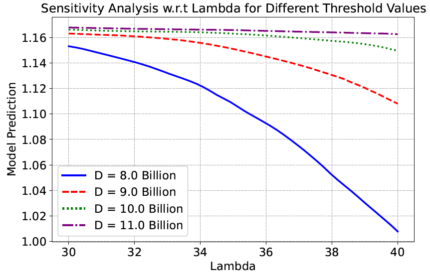
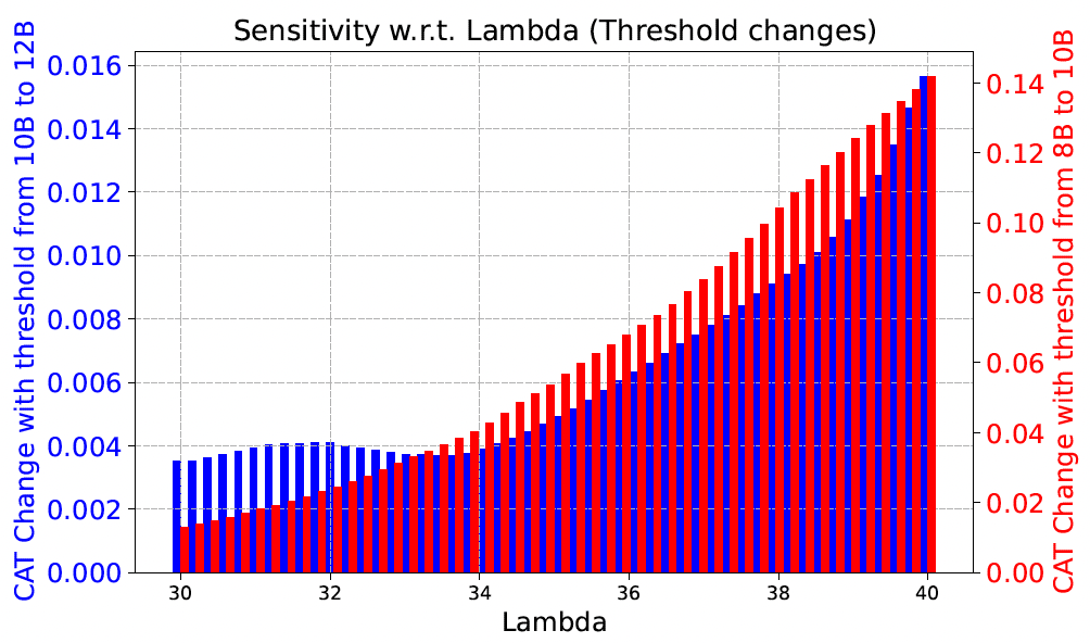
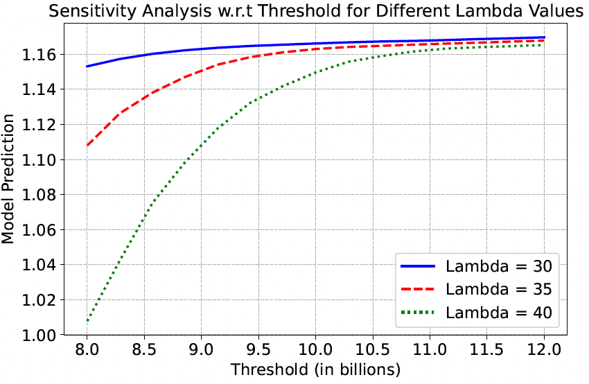
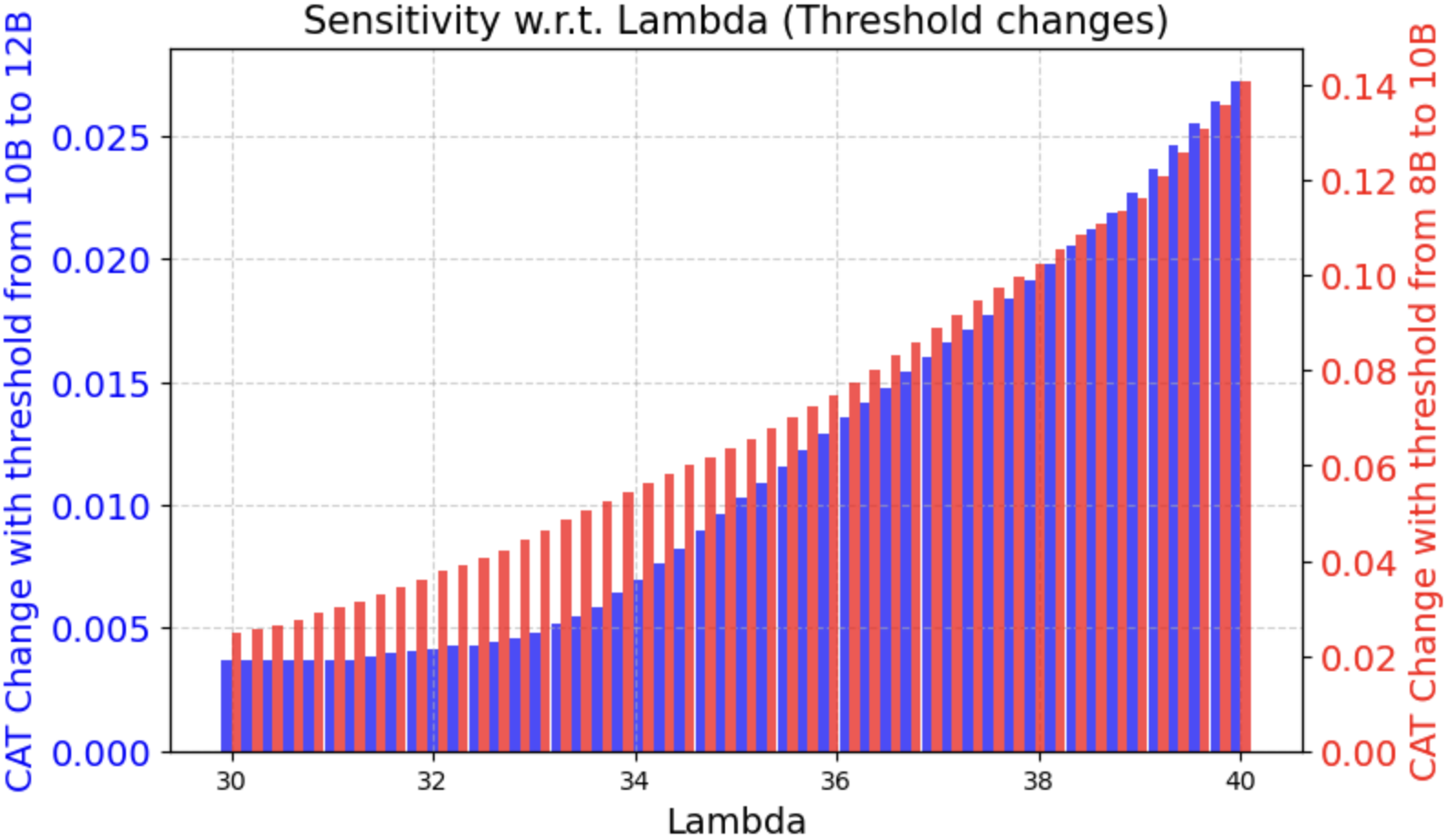
The trained pricing map also gives immediate sensitivity curves. Figures 2 and 3 vary catastrophe intensity, attachment threshold, and the initial short rate under Gamma and Lognormal severities. These curves are evaluations of the same surrogate, not separate models.
The results match the economics of CAT bond risk. Prices decline with catastrophe intensity because more frequent arrivals raise the probability of principal impairment; the effect is steepest at low attachment thresholds and much flatter when billion. Prices move in the opposite direction with the threshold: increasing makes the trigger harder to reach, with the strongest marginal effect around 8–9 billion dollars where the trigger probability changes most rapidly. Prices also decline with the initial short rate , consistent with higher discount rates lowering present values, while the shape of this rate response is only weakly affected by . The figures therefore serve both as validation and as a risk-management output. They show economically correct monotonicities, identify nonlinear regions where contract design matters most, and provide full response curves without recomputing rare-event simulations on a grid. This analysis directly links the speed gain of the presented method to a risk-management use case: each curve requires many valuations, which would otherwise require repeated rare-event simulations. A finite-difference monotonicity check on dense grids is reported in the supplementary material, with violation rates. The results show 0% monotonicity violation rates for , , and under both the Gamma and Lognormal severity models, confirming that the neural network preserves the expected monotonic relationships across the parameter domain.





5 Conclusion
A neural surrogate turns structural CAT bond valuation into a real-time finance tool for repeated in-domain valuation. It preserves the interpretability of a compound-Poisson pricing model while amortizing the cost of rare-event simulation across future valuations. The empirical results show small out-of-sample pricing errors on the simulated domain, value estimates close to MC-IS benchmarks, and speed gains large enough to support screening and sensitivity analysis. The method is best viewed as a fast engine conditional on a chosen pricing measure, severity model, and trigger specification. Future work should combine the surrogate with market calibration, multi-peril dependence, richer trigger structures, and portfolio-level risk aggregation.
Acknowledgments
The authors thank Prabhav Kumar for valuable input during the early stages of this work. J. Sester gratefully acknowledges support by the NUS Start-Up Grant Tackling model uncertainty in Finance with machine learning, by the MOE AcRF Tier 1 Grant 25-0428-P0001, and by the MOE AcRF Tier 2 Grant T2EP20225-0030.
Data and code availability
The reported results are based on simulated data generated from the model and parameter ranges described in the paper and supplementary material. No proprietary data were used. The replication code, training configurations, seeds, and notebooks are available at https://github.com/HuansangXu/CAT-bonds.
Declaration of generative AI and AI-assisted technologies in the manuscript preparation process
During manuscript preparation, the authors used ChatGPT to assist with shortening and editorial rewriting. The authors reviewed and edited the content and take full responsibility for the submitted manuscript.
Appendix: Supplementary material
This supplement collects the technical statements, algorithms, proofs, and numerical diagnostics from the original manuscript. It is intended to be read alongside the main paper. In particular, Section C justifies the neural-network approximation by applying the universal approximation theorem to the CAT-bond pricing map on compact parameter sets. Sections B–B.2 explain the importance-sampling construction used to generate training labels, while the proofs of Propositions B.1 and B.2 give the corresponding mathematical variance-reduction arguments for Gamma and Lognormal severity specifications. Section D reports additional diagnostics including boundary-region errors, MC-IS benchmark settings, offline computational costs, monotonicity checks, and architecture robustness.
Appendix A Model and pricing statements
A.1 Modeling interest rates
Consider a probability space , where is interpreted as a risk-neutral probability measure, or spot martingale measure, and let be a sub-filtration of , describing the evolution of available market information over time. In line with [6, 9, 8, 17, 20], we use a general affine term structure model to model the spot interest rate, i.e., we assume the annual interest rate has dynamics
| (A.1) |
for denoting a standard Brownian motion w.r.t. , meaning that the drift and variance rate are affine in the spot rate at all times – explaining the name of this model class.
A non-defaultable zero coupon bond promises the payment of the face value at maturity . Assuming no default risk, by risk-neutral valuation (see, e.g., [36]), the price of the zero coupon bond at time is given by
| (A.2) |
where the last equality follows from our assumption of an affine term structure, see also, e.g., [17]. and are deterministic functions of the model parameters which satisfy the ordinary system of equations:
| (A.3) | ||||
see, e.g., [33, 17]. In order to ensure the existence of continuous solutions and we impose the following assumption.
Assumption A.1.
The coefficient functions , , , from (A.1) are assumed to be continuous.
Lemma A.2.
A.2 Pricing of CAT bonds
Given the rare and unpredictable nature of catastrophic events, Poisson processes provide a natural mathematical framework for CAT bond pricing. In this approach, the jumps of the Poisson process correspond to catastrophe occurrences, with the jump frequency parameter capturing the rate at which catastrophes occur. This modeling choice has become the standard approach in the literature, as demonstrated in the comprehensive review by [56], which examines various CAT bond pricing methodologies.
To describe these catastrophes mathematically, we model the number of catastrophes by a -conditional Poisson process , defined on , associated with positive intensity being a -progressively measurable process with locally integrable sample path.
This allows to define a hazard process , which is -adapted, right-continuous and increasing. For any and every , we then have
Next, we model the indemnity loss trigger. The th occurrence of a loss is given by a value drawn from the random variable . For tractability, we assume that the losses { are independent and identically distributed (i.i.d.) with cumulative distribution function (cdf) and independent of . Then, the aggregate indemnity loss is a compound Poisson process such that
A trigger event occurs exactly when exceeds some pre-determined threshold , i.e., we are considering the stopping time indicating a loss event. We define by , where denotes the indicator function if , and otherwise, and we observe that is itself a doubly stochastic Poisson process, see also [30].
Lemma A.3.
The process is a doubly stochastic Poisson process with intensity .
This result leads directly to the following pricing formulas.
Corollary A.4.
Consider a CAT-bond at time with face value , maturity , and loss threshold .
-
(i)
The (risk-neutral) price of a zero-coupon CAT bond that pays at maturity only if no trigger event occurs by time is given by
(A.4) -
(ii)
The (risk-neutral) price of a CAT bond with face value , maturity , and coupon payments at times where , is given by
(A.5) -
(iii)
If, in the setting of (ii), the CAT bond has a recovery rate , then its (risk-neutral) price is
(A.6)
Appendix B Monte Carlo and importance sampling statements
B.1 Monte Carlo integration
According to (A.4), prices of CAT bonds can be understood as a combination of zero coupon bond price and the expectation introducing path dependency, and thus imposing an additional numerical challenge. Due to Lemma A.2, an explicit solution for the zero coupon bond price according to Eq. (A.2) is readily available, however, in general there is no closed-form analytical solution for , so thus . Instead, a numerical approximation, e.g., via Monte Carlo integration is required to evaluate this expectation. Alternatively, leveraging the Feynman–Kac theorem (see, e.g., [40]), integro-PDE methods could be applied (see, e.g., [30]), which are used as a benchmark in the main manuscript.
To determine CAT bond prices at time , due to (A.4), we need to compute the risk-neutral probability of a trigger event that corresponds to .
We approximate this probability using Monte Carlo simulation. For a fixed number of simulations , we generate independent loss realizations and compute the estimator
for denoting the loss in the th simulation. The variance of the estimated trigger probability is given as
Algorithm 1 in the appendix outlines the procedure to compute this estimate.
B.2 Importance sampling
By the law of large numbers, converges to as the sample size increases. Although the MC estimator converges to , plain Monte-Carlo estimation is characterized by slow convergence and a large variance, since for large thresholds , very few samples contribute to the estimate, see also, e.g., [55]. This motivates to apply Importance Sampling (IS), a variance reduction technique allowing to sample under a different probability measure making exceedance of the threshold a more frequently occurring event. To this end, we consider a second probability density , whose support is assumed to contain that of original density , and define the likelihood ratio by whenever , and otherwise. Hence, we get .
The idea of using IS is to choose the density such that Monte-Carlo simulation under leads to an IS estimator with variance being smaller than for the standard Monte Carlo integration. Then, we estimate , where is simulated according to density , is the indicator function associated to the trigger event and denotes the likelihood ratio used for the change of measure in the th simulation. We compute that the variance for the estimated trigger probability equals
To determine a candidate change of measure for IS in the compound Poisson setting, we follow the procedure outlined in [55, Chapter 7], [43, Chapter 11.4 ], [34], or [50, Section 3], by applying exponential tilting. For the aggregated loss , two types of random variables need to be simulated - the number of losses and the size of losses. Firstly, consider the number of losses till time , modelled by a Poisson process with intensity . The moment generating function (MGF) of is calculated to be
where is defined in Section A.2. Applying exponential tilting that changes the probability measure from to for , we have
The number of losses under probability measure is thus modelled by a Poisson process with new intensity after having applied exponential tilting.
Next, we address the jump size component. Catastrophic losses typically exhibit heavy-tailed behavior, necessitating appropriate distributional choices. The actuarial literature has identified several continuous distributions suitable for modeling such extreme losses. Among these, the Gamma and Lognormal distributions have emerged as particularly popular choices, though other options include the Pareto and Burr distributions, compare, also [38]. In the following subsections, we develop specific IS techniques for both the Gamma and Lognormal distributions.
B.2.1 Importance sampling for Gamma distributed losses
We first consider Gamma distributed losses. Assume the size of losses are i.i.d. according to a Gamma distribution with shape and scale , i.e., its probability density function is given as
Applying exponential tilting, we have that the new density function for the size of losses under the new probability measure is given by
for , see, e.g., [29]. This means the jump size satisfies a Gamma distribution with shape and new scale under the probability measure .
Recall, that the initial mean value of the losses is usually much smaller than the predetermined threshold , i.e., we have , leading to a high variance of standard Monte Carlo estimates. For IS, we select parameters and such that the expected value of the loss under the modified measure approximates the threshold , i.e., . By this choice the event will occur much more frequently which in turn helps to reduce the variance of the estimators. To this end, note that the expected loss under computes as
| (B.1) |
where the first equality follows from Wald’s identity.
From Eq. (B.1), it is evident that the choice of the importance sampling parameters plays a critical role in reducing the variance of the estimated trigger probability, which is the primary objective of importance sampling. While one may rely on numerical experimentation to evaluate various combinations of and select the most effective pair for a given loss distribution, this approach lacks generality and may not guarantee robustness across different scenarios. Therefore, it is important to investigate the regularity and consistency of this parameter selection procedure. Below, we present a result that guides the appropriate selection of across a broad class of loss distributions allowing for a more systematic and reliable guidance than case-by-case numerical tuning.
Proposition B.1.
Let an aggregate indemnity loss be defined by , where and are i.i.d. with for . Further, let
Then, the importance sampling estimator with
satisfies
IS is most beneficial when estimating probabilities of rare events, particularly when the expected loss under the original measure is significantly smaller than the threshold, i.e., when . When the maturity is large, the aggregate indemnity loss increases, leading to a higher trigger probability, making it not necessarily a rare event anymore. In such scenarios, one can use standard Monte Carlo simulation with a reasonable small variance instead.
In the appendix, we provide Algorithm 2 to estimate the trigger probability with Gamma distributed losses by using Monte Carlo simulation with IS.
B.2.2 Importance sampling for Lognormally distributed losses
Now we consider another frequently used type of loss distribution - the Lognormal distribution. Assume the size of losses are i.i.d. and satisfy a Lognormal distribution with parameters (mean of ) and (standard deviation of ). The probability density function of the random variable is
The moment generating function of a Lognormal distribution is infinite for positive arguments. Thus, we cannot apply exponential tilting for Lognormal distributions directly. Instead, we follow the idea from [31], where the importance sampling density is built as another Lognormal distribution with a larger expected value, denote as under the probability measure , with . Analogue to Eq. (B.1), we compute the expected loss under , and obtain
| (B.2) |
Due to the complexity and heavy-tailed nature of the Lognormal distribution, it is not feasible to directly propose suitable IS parameters for Lognormal losses. While in the Gamma case explicit IS parameters can be derived through Proposition B.1, the Lognormal setting requires a different strategy. Therefore, we adopt a variance minimization approach to determine the optimal IS parameters for Lognormal distributed losses. Further, recall that the variance of IS estimator is given as
and hence our goal is minimize . Under we have and . Thus, we can compute the likelihood ratio under the measure after IS as follows:
| (B.3) |
By minimizing the expectation , we get the following result
Proposition B.2.
Let an aggregate indemnity loss be defined by , where and with . Set such that
where and are the pdf and cdf of the standard normal distribution, respectively. Then for large enough, the variance of the importance sampling estimator with as in (B.3) satisfies
The optimal pushes the log-severity mean close to , then follows from to keep the Poisson weight balanced. Algorithm 3 for estimating the trigger probability with Lognormally distributed losses by using Monte Carlo simulation with IS is provided in the appendix.
Having established the Monte Carlo simulation algorithms, we can utilize the estimated trigger probability in conjunction with the zero-coupon bond price from Eq. (A.2) under an affine term structure interest rate model. By incorporating these components into the CAT bond pricing formula in Eq. (A.5), we can determine the CAT bond price under various parameter settings. The complete calculation procedure is outlined in Algorithm 4.
Appendix C Pricing CAT bonds with neural networks
C.1 Feedforward neural networks
The following exposition on neural networks (NNs) is borrowed from [52] but can be found in a similar form in any standard textbook on the topic, e.g., [44] or [53]. By fully-connected feedforward neural networks, or simply neural networks with input dimension , output dimension , and number of layers we refer to functions of the form
| (C.1) | ||||
where are affine222This means for all , the function is assumed to have an affine structure of the form for some matrix and some vector , where and . functions of the form
| (C.2) |
and where the function is applied componentwise, i.e., for we have . The function is called activation function and assumed to be continuous and non-polynomial. Here denotes the dimensions (the number of neurons) of the hidden layers, also called hidden dimension.
Then, we denote by the set of all neural networks with input dimension , output dimension , hidden layers, and hidden dimension , whereas the set of all neural networks from to (i.e. without specifying the number of hidden layers and hidden dimension) is denoted by
It is well-known that the set of neural networks possesses the so-called universal approximation property, see, e.g., [45] or [21].
Proposition C.1 (Universal approximation theorem).
For any compact set the set is dense in with respect to the topology of uniform convergence on .
By using Proposition C.1 we can show that neural networks are able to approximate CAT bond prices arbitrarily well after being trained. Firstly, recalling the pricing formula for the zero coupon CAT bond Eq. (A.4), we assume that the Poisson intensity is fixed over time that and then we set to emphasize its dependence on the initial interest rate , the Poisson intensity and the trigger threshold .
Proposition C.2.
Let Assumption A.1 hold true, let be a compact set and let the loss distribution of follow a continuous distribution. Then for all , there exists a fully connected feedforward neural network such that for all
According to Eq. (A.5), the coupon CAT bond price is the cumulative sum of zero coupon CAT bonds with face value and s, each at the respective maturity. Hence, we directly get the following proposition showing that the coupon CAT bond price in Eq. (A.5) can be approximated arbitrarily well by neural networks whenever we restrict the inputs to a compact set. In order to emphasize the dependence of the coupon CAT bond price on the payment schedule , the initial interest rate , the Poisson intensity and the threshold , we set
Proposition C.3.
Let Assumption A.1 hold true. Given , let be a compact set and let the loss distribution of follow a continuous distribution. Then for all , there exists a fully connected feedforward neural network such that for all
Appendix D Additional numerical diagnostics and reproducibility details
D.1 Operational domain, boundary regions, and extrapolation
The training design in the main manuscript defines the operational training domain
where the coordinates are and is measured in days. The neural-network surrogate is therefore assessed as an interpolator on this compact set. It is not used as a validated extrapolation rule outside . For out-of-domain contracts, the recommended procedure is to enlarge the simulation design and retrain, or to fall back to direct MC-IS valuation.
For each continuous coordinate , where and are the lower and upper bounds of the training domain, respectively, we define the boundary subset as the set of points whose -th coordinate lies within the outermost of the interval near either boundary:
For the coupon-count coordinate, the boundary subset is . Table 3 reports pricing errors on these held-out boundary subsets demonstrating only a slight deterioration of accuracy near the boundaries.
| Severity | Test subset | Observations | MAE | RMSE | Max. AE |
|---|---|---|---|---|---|
| Gamma | Full test set | 120000 | 0.00274 | 0.00380 | 0.02556 |
| Gamma | boundary | 11877 | 0.00304 | 0.00408 | 0.02108 |
| Gamma | boundary | 12007 | 0.00291 | 0.00404 | 0.02348 |
| Gamma | boundary | 11864 | 0.00305 | 0.00413 | 0.02391 |
| Gamma | boundary | 12063 | 0.00328 | 0.00447 | 0.02324 |
| Gamma | 30080 | 0.00296 | 0.00407 | 0.02556 | |
| Lognormal | Full test set | 120000 | 0.00308 | 0.00429 | 0.03296 |
| Lognormal | boundary | 12081 | 0.00345 | 0.00464 | 0.03296 |
| Lognormal | boundary | 12265 | 0.00328 | 0.00463 | 0.03296 |
| Lognormal | boundary | 11822 | 0.00328 | 0.00456 | 0.03296 |
| Lognormal | boundary | 11880 | 0.00366 | 0.00499 | 0.02918 |
| Lognormal | 29941 | 0.00333 | 0.00470 | 0.03296 |
D.2 Expanded out-of-sample accuracy diagnostics
Table 4 complements Figure 1 in the main manuscript. Besides MAE and MSE, it reports signed bias, RMSE, high absolute-error quantiles, maximum absolute error, and on the held-out test set.
| Severity | Observations | Bias | MAE | MSE | RMSE | 95% AE | 99% AE | |
|---|---|---|---|---|---|---|---|---|
| Gamma | 120000 | 0.00026 | 0.00274 | 0.00380 | 0.00808 | 0.01286 | 0.99989 | |
| Lognormal | 120000 | 0.00009 | 0.00308 | 0.00429 | 0.00928 | 0.01413 | 0.99984 |
D.3 MC-IS benchmark protocol and offline computational cost
For the timing benchmark in the main manuscript, MC-IS is run under a fixed and reproducible protocol. Each protected coupon date and the principal date are priced by estimating the corresponding trigger probability with the same importance-sampling construction as in Section B.2. The comparison is therefore between a direct MC-IS valuation of each requested contract and evaluation of the already-trained surrogate.
| Item | Specification |
|---|---|
| Paths per trigger-probability estimate | 5,000 importance-sampling paths |
| Stopping/convergence rule | Fixed number of Monte Carlo simulations |
| Random seeds | NumPy random seed = 125 |
| Common random numbers across methods | No. The surrogate evaluation is deterministic. |
| Hardware for timing experiments | Apple M3 Pro |
| Software stack | Python 3.12.2, NumPy 1.26.4, SciPy 1.13.1, TensorFlow 2.18.0 |
The neural-network timings in the main manuscript are online evaluation times. Table 6 records the corresponding one-time offline costs. These costs are incurred once for a fixed model specification, severity law, and input domain, and are amortized when the trained pricing surface is queried repeatedly.
| Task | Specification | Wall-clock time |
|---|---|---|
| Label generation | Gamma severities, 600,000 prices | 24 h 21 min |
| Label generation | Lognormal severities, 600,000 prices | 33 h 20 min |
| Training | Architecture , Gamma Lognormal | 21.55 min |
| Training | Architecture , Gamma | 29.70 min |
| Training | Architecture , Lognormal | 35.98 min |
| Training | Architecture , Gamma Lognormal | 81.62 min |
| Full cross-validation | All candidate architectures and folds | 7 h 27 min |
Note. Full cross-validation evaluates four candidate configurations for each severity distribution (Gamma and Lognormal), obtained by combining two hidden-layer architectures, and , with two learning rates, and . The activation function (ReLU), L2 regularization coefficient (), dropout rate (), and batch normalization are kept fixed throughout.
D.4 Economic monotonicity diagnostics
The structural model implies economically expected signs on the training domain: prices should be non-increasing in the catastrophe intensity , non-decreasing in the attachment threshold , and non-increasing in the initial short rate for positive protected cash flows. We quantify whether the learned surrogate violates these signs on a dense finite-difference grid. With tolerance , a violation is recorded if
where each difference compares adjacent grid values while holding the other inputs fixed.
In the following Table 7, we evaluate the model on dense uniform grids consisting of 100,001 points for each parameter: , , and , which include samples out of the training domain. The table shows that no violations of the monotonicity relations can be observed.
| Severity | Variable | Expected sign | Grid comparisons | Violation rate | Max. violation |
|---|---|---|---|---|---|
| Gamma | non-increasing | 100000 | 0% | 0 | |
| Gamma | non-decreasing | 100000 | 0% | 0 | |
| Gamma | non-increasing | 100000 | 0% | 0 | |
| Lognormal | non-increasing | 100000 | 0% | 0 | |
| Lognormal | non-decreasing | 100000 | 0% | 0 | |
| Lognormal | non-increasing | 100000 | 0% | 0 |
D.5 Stability to architecture selection
Table 8 reports the performance of alternative architectures considered during model selection. The goal is not to claim that the selected architecture is unique, but to show whether valuation accuracy is stable across nearby depth/width choices.
| Severity | Architecture | Parameters | MAE | MSE | Training time |
|---|---|---|---|---|---|
| Gamma | 11,137 | 0.00331 | 653.69 s | ||
| Gamma | 44,801 | 0.00274 | 1782.01 s | ||
| Gamma | 175,617 | 0.00317 | 2286.54 s | ||
| Lognormal | 11,137 | 0.00379 | 639.37 s | ||
| Lognormal | 44,801 | 0.00308 | 2158.52 s | ||
| Lognormal | 175,617 | 0.00309 | 2610.53 s |
Note. The parameter counts are trainable parameters reported by the final Keras model summary. All models use identical hyperparameters: ReLU activation, L2 regularization coefficient , dropout rate , batch normalization, and learning rate . Only the hidden-layer architecture varies.
Appendix E Algorithms
In this section, we present all the algorithms used. Implementations of the algorithms can be found for the convenience of the reader, and for reproducibility of the results, under https://github.com/HuansangXu/CAT-bonds.
Appendix F Proofs
F.1 Proof of Lemma A.2
Proof of Lemma A.2.
We begin by considering the first line of (A.3), i.e., the Riccati-type ordinary differential equation (ODE) describing the dynamics of :
Since and are continuous by Assumption A.1, standard results on Riccati equations guarantee existence of a unique and continuous solution for fixed , see, e.g., [46].
We now investigate the continuity of with respect to the maturity parameter . Let , and define for fixed the difference
We compute the derivative of with respect to using the ODE satisfied by both and :
| (F.1) | ||||
Next, we define
and apply Grönwall’s inequality to (F.1), which implies:
| (F.2) |
We then observe that
which is finite because , , , and are all continuous, and hence is bounded on . Note that by definition,
since by the boundary condition of the Riccati ODE (A.3). As the solution is continuous, we have
with . Thus, (F.2) gives
which tends to zero as . Therefore, is continuous in the maturity . Next, we want to show that is continuous with respect to the maturity . Consider the defining ODE for
where and are assumed to be continuous functions and is known to be continuous in from the above result. Thus, a unique continuous solution exists for any . Fix , and define the difference of and ,
and hence, since and all are continuous we obtain for all , showing the continuity of in . ∎
F.2 Proof of Lemma A.3
Proof of Lemma A.3.
According to the definition of doubly stochastic Poisson processes, see, e.g., [41], we need to show that for the following two properties are fulfilled.
-
1.
,
-
2.
,
or equivalently
-
(1′)
,
-
(2′)
.
We start by showing (2). Let , and consider the time interval for small . Then, we compute
| (F.3) |
Next, we show property (1). Using the above Equation (F.3), we get
| (F.4) |
∎
F.3 Proof of Corollary A.4
Proof of Corollary A.4.
-
(i)
By risk-neutral valuation333Compare the exposition in [32] for the analogue situation of credit sensitive bonds., the arbitrage-free price of a zero coupon CAT bond with face value and maturity at time is given by
(F.5) where the last equality is due to Lemma A.3 and the properties of doubly stochastic Poisson processes.
-
(ii)
After we get the price of zero-coupon CAT bond from (1), the price of a coupon CAT bond can be formed directly by considering each coupon payment at time for and by using linearity of the expectation.
-
(iii)
The price of a CAT bond with face value , maturity , coupon payments at time for , where , and recovery rate at time is
(F.6)
∎
F.4 Proof of Proposition B.1
Proof of Proposition B.1.
First note that follows directly from definition. Moreover, recall that the variance of estimated trigger probability under standard Monte Carlo simulation and under IS is given by
Thus, comparing with reduces to comparing with . Note that the likelihood ratio for the Poisson process when applying exponential tilting is
First, consider . The likelihood ratio of computes as
The condition writes equivalently as
| (F.7) |
Thus, by (B.1), (F.7), and through setting which is equivalent to , we obtain
| (F.8) |
Note that the likelihood ratio for the compound Poisson process computes now as
Taking the expectation, we obtain the bound:
To simplify the first factor of the above expression we use (F.7), (F.8), and the inequality of arithmetic and geometric means 444AM - GM inequality: for two non-negative numbers and , with equality if and only if . applied to to obtain
Hence, . For the second factor, applying (F.7) and (F.8) gives
Altogether, we have
which provides if losses are Gamma distributed.
∎
F.5 Proof of Proposition B.2
Proof of Proposition B.2.
First note that follows directly from the definition of the estimators. Our goal is to minimize to find the optimal IS parameters and , where
| (F.9) |
To get rid of the last factor in (F.9), we consider an additional change of measure from the original measure to measure so that under measure . We compute the likelihood ratio
| (F.10) | ||||
Then we can rewrite the conditional expectation under the new measure as
| (F.11) | ||||
Instead of minimizing the conditional expectation directly and comparing with , we minimize its ratio .
Note that by the properties of subexponential distributions (to which the Lognormal distribution belongs), we have for all ,
| (F.12) |
see, e.g., Chapter VI, Section 3 in [29]. Next, let and choose such that
Due to (F.12) there exists some such that for all and for all with we have
This implies for all
where is the cdf of the standard normal distribution. In the above inequalities, we used for all , that for , and that . Now, by using (F.11), we derive an upper bound for our minimization problem by
| (F.13) |
for some constant when restricting to and where and are chosen sufficiently large. To minimize , we will minimize its upper bound which reduces to minimizing . To simplify the analysis, we define
| (F.14) |
Start by fixing , and minimize the function with respect to . The first order condition writes as
Next, we verify
which confirms that is indeed the global minimizer of for any fixed . Next, we substitute back into function and find the optimal . To this end, we define
and we minimize the function . The first order condition becomes
where and are the pdf and cdf of the standard normal distribution. To verify the second order condition, we compute
where . This second derivative of function involves the Mills ratio:
so we can rewrite
according to standard properties of the Mills ratio, see, e.g., [48, Chapter 13]. Thus, we have
which confirms that is the global minimizer of .
Finally, substituting the optimal values and into the function , we obtain
We conclude by letting .
∎
F.6 Proof of Proposition C.2
Proof of Proposition C.2.
We need to show that the map
is continuous. Then, the assertion follows with Proposition C.1. Firstly, we see that depends on the face value and initial interest rate only through , which by Eq. (A.2) is given as
and which is continuous in and , so thus . Moreover, is continuous in according to Lemma A.2. Define the integral term:
where the last equality follows by Fubini’s Theorem. As by Corollary A.4, the CAT bond price can be written as
we obtain that is continuous in and in . Finally, for the continuity in , let , and we aim at proving the existence of such that
| (F.15) |
Without loss of generality, we assume , and we define
Then we can compute the difference
| (F.16) |
Note that , and we see that for any
Next, one can find such that implies
Thus, we have
Since is a cumulative density function for some continuous distribution , we have . Then applying Fubini’s Theorem to the second term in (F.6), we have
Moreover, as is continuous for all , there exists such that yields
Thus implies
∎
Proof of Proposition C.3.
Firstly, we have is continuous in , according to Proposition C.2. Similarly, for each coupon payment dates , for , the discounted coupon payments is continuous in and does not depend on any other inputs. Recall the formula of coupon CAT bond price that
it is a cumulative sum of and . We can conclude that is continuous in and the universal approximation theorem from Proposition C.1 can be applied. ∎
References
- Artemis [2024] Artemis, 2024. Catastrophe bonds and insurance-linked securities issuance and outstanding market dashboard.
- Baryshnikov et al. [2001] Baryshnikov, Y., Mayo, A., Taylor, D.R., 2001. Pricing of CAT bonds. Preprint.
- Burnecki and Kukla [2003] Burnecki, K., Kukla, G., 2003. Pricing of zero-coupon and coupon CAT bonds. Applicationes Mathematicae 30, 315–324.
- Braun and Kousky [2021] Braun, A., Kousky, C., 2021. Wharton Risk Center primer: Catastrophe bonds. Wharton Risk Management and Decision Processes Center, University of Pennsylvania.
- Chen et al. [2026] Chen, H., Didisheim, A., Scheidegger, S., 2026. Deep surrogates for finance: With an application to option pricing. Journal of Financial Economics 177, 104222.
- Cuchiero et al. [2010] Cuchiero, C., Teichmann, J., Filipovic, D., 2010. Affine models. Encyclopedia of Quantitative Finance.
- Cybenko [1989] Cybenko, G., 1989. Approximation by superpositions of a sigmoidal function. Mathematics of Control, Signals and Systems 2, 303–314.
- Duffee [2002] Duffee, G.R., 2002. Term premia and interest rate forecasts in affine models. Journal of Finance 57, 405–443.
- Duffie and Kan [1996] Duffie, D., Kan, R., 1996. A yield-factor model of interest rates. Mathematical Finance 6, 379–406.
- Glasserman [2004] Glasserman, P., 2004. Monte Carlo Methods in Financial Engineering. Springer.
- Hardle and Lopez Cabrera [2010] Härdle, W.K., Lopez Cabrera, B., 2010. Calibrating cat bonds for Mexican earthquakes. Journal of Risk and Insurance, 77(3), 625–650.
- Hofer et al. [2021] Hofer, L., Gardoni, P., Zanini, M.A., 2021. Risk-based cat bond pricing considering parameter uncertainties. Sustainable and Resilient Infrastructure 6, 315–329.
- Hornik et al. [1989] Hornik, K., Stinchcombe, M., White, H., 1989. Multilayer feedforward networks are universal approximators. Neural Networks 2, 359–366.
- Horvath et al. [2021] Horvath, B., Muguruza, A., Tomas, M., 2021. Deep learning volatility: A deep neural network perspective on pricing and calibration in (rough) volatility models. Quantitative Finance 21, 11–27.
- Hutchinson et al. [1994] Hutchinson, J.M., Lo, A.W., Poggio, T., 1994. A nonparametric approach to pricing and hedging derivative securities via learning networks. The Journal of Finance 49, 851–889.
- Jarrow [2010] Jarrow, R.A., 2010. A simple robust model for CAT bond valuation. Finance Research Letters 7, 72–79.
- Keller-Ressel et al. [2011] Keller-Ressel, M., Schachermayer, W., Teichmann, J., 2011. Affine processes are regular. Probability Theory and Related Fields 151, 591–611.
- Liu et al. [2019] Liu, S., Oosterlee, C.W., Bohte, S.M., 2019. Pricing options and computing implied volatilities using neural networks. Risks 7, 16.
- Neufeld and Sester [2022] Neufeld, A., Sester, J., 2022. A deep learning approach to data-driven model-free pricing and to martingale optimal transport. IEEE Transactions on Information Theory 69, 3172–3189.
- Piazzesi [2010] Piazzesi, M., 2010. Affine term structure models. In: Handbook of Financial Econometrics: Tools and Techniques. Elsevier, 691–766.
- Pinkus [1999] Pinkus, A., 1999. Approximation theory of the MLP model in neural networks. Acta Numerica 8, 143–195.
- Polacek [2018] Polacek, A., 2018. Catastrophe bonds: A primer and retrospective. Chicago Fed Letter 405, 1–7.
- Reshetar [2008] Reshetar, G., 2008. Pricing of multiple-event coupon paying cat bond. SSRN working paper.
- Ruf and Wang [2020] Ruf, J., Wang, W., 2020. Neural networks for option pricing and hedging: A literature review. Journal of Computational Finance 24, 1–46.
- Siyamah et al. [2021] Siyamah, I., Putri, E.R.M., Imron, C., 2021. CAT bond valuation using Monte Carlo and quasi Monte Carlo method. Journal of Physics: Conference Series 1821, 012053.
- Sukono et al. [2022] Sukono, Juahir, H., Ibrahim, R.A., Saputra, M.P.A., Hidayat, Y., Prihanto, I.G., 2022. Application of compound Poisson process in pricing catastrophe bonds: A systematic literature review. Mathematics 10, 2668.
- Vasicek [1977] Vasicek, O.A., 1977. An equilibrium characterization of the term structure. Journal of financial economics, 5(2), 177–188.
- Polacek [2018] Polacek, A., 2018. Catastrophe bonds: A primer and retrospective. Chicago Fed Letter 405, 1–7.
- Asmussen and Glynn [2007] Asmussen, S., Glynn, P.W., 2007. Stochastic Simulation: Algorithms and Analysis. Springer.
- Baryshnikov et al. [2001] Baryshnikov, Y., Mayo, A., Taylor, D.R., 2001. Pricing of CAT bonds. Working paper.
- Bee [2009] Bee, M., 2009. Importance sampling for sums of lognormal distributions with applications to operational risk. Communications in Statistics - Simulation and Computation 38, 939–960.
- Bielecki and Rutkowski [2013] Bielecki, T.R., Rutkowski, M., 2013. Credit Risk: Modeling, Valuation and Hedging. Springer.
- Bjork [2009] Bjork, T., 2009. Arbitrage Theory in Continuous Time. Oxford University Press.
- Blanchet and Zwart [2007] Blanchet, J., Zwart, B., 2007. Importance sampling of compounding processes. Winter Simulation Conference, 372–379.
- Braun and Kousky [2021] Braun, A., Kousky, C., 2021. Catastrophe bond. Wharton Risk Center Primer.
- Brigo and Mercurio [2006] Brigo, D., Mercurio, F., 2006. Interest Rate Models: Theory and Practice. Springer.
- Burnecki et al. [2019] Burnecki, K., Giuricich, M.N., Palmowski, Z., 2019. Valuation of contingent convertible catastrophe bonds: The case for equity conversion. Insurance: Mathematics and Economics 88, 238–254.
- Burnecki and Kukla [2003] Burnecki, K., Kukla, G.T., 2003. Pricing of zero-coupon and coupon cat bonds. Applicationes Mathematicae 30, 315–324.
- Cizek et al. [2011] Cizek, P., Hardle, W., Weron, R., 2011. Statistical Tools for Finance and Insurance. Springer.
- Cont and Tankov [2003] Cont, R., Tankov, P., 2003. Financial Modelling with Jump Processes. Chapman and Hall/CRC.
- Cox and Isham [1980] Cox, D.R., Isham, V., 1980. Point Processes. CRC Press.
- Cox et al. [1985] Cox, J.C., Ingersoll, J.E., Ross, S.A., 1985. A theory of the term structure of interest rates. Econometrica 53, 385–407.
- Embrechts et al. [2015] Embrechts, P., Frey, R., McNeil, A., 2015. Quantitative Risk Management: Concepts, Techniques and Tools. Princeton University Press.
- Goodfellow et al. [2016] Goodfellow, I., Bengio, Y., Courville, A., 2016. Deep Learning. MIT Press.
- Hornik et al. [1989] Hornik, K., Stinchcombe, M., White, H., 1989. Multilayer feedforward networks are universal approximators. Neural Networks 2, 359–366.
- Ince [2012] Ince, E.L., 2012. Ordinary Differential Equations. Dover Publications.
- Jarrow [2010] Jarrow, R.A., 2010. A simple robust model for CAT bond valuation. Finance Research Letters 7, 72–79.
- Johnson et al. [1995] Johnson, N.L., Kotz, S., Balakrishnan, N., 1995. Continuous Univariate Distributions, Vol. 2. Wiley.
- Kingma [2014] Kingma, D.P., 2014. Adam: A method for stochastic optimization. arXiv:1412.6980.
- Lutkebohmert and Sester [2025] Lutkebohmert, E., Sester, J., 2025. Measuring name concentrations through deep learning. International Review of Financial Analysis 107, 104598.
- Ma and Ma [2013] Ma, Z., Ma, C., 2013. Pricing catastrophe risk bonds: A mixed approximation method. Insurance: Mathematics and Economics 52, 243–254.
- Neufeld and Sester [2024] Neufeld, A., Sester, J., 2024. Neural networks can detect model-free static arbitrage strategies. Applied Mathematics and Optimization 90, 41.
- Nielsen [2015] Nielsen, M.A., 2015. Neural Networks and Deep Learning. Determination Press.
- Nowak and Romaniuk [2018] Nowak, P., Romaniuk, M., 2018. Valuing catastrophe bonds involving correlation and CIR interest rate model. Computational and Applied Mathematics 37, 365–394.
- Glasserman [2004] Glasserman, P., 2004. Monte Carlo Methods in Financial Engineering. Springer.
- Sukono et al. [2022] Sukono, Juahir, H., Ibrahim, R.A., Saputra, M.P.A., Hidayat, Y., Prihanto, I.G., 2022. Application of compound Poisson process in pricing catastrophe bonds: A systematic literature review. Mathematics 10, 2668.
- Vasicek [1977] Vasicek, O.A., 1977. An equilibrium characterization of the term structure. Journal of Financial Economics 5, 177–188.