references.bib\orcid0009-0009-1806-2166\orcid0000-0002-3869-4023\orcid0009-0004-9769-7250\publicationstatusPreprint \version6.0 \preprintdateJuly 2026
Synthetic Homes: A Multimodal Generative AI Pipeline for Residential Building Data Generation under Data Scarcity
Abstract
Computational models have emerged as powerful tools for multi-scale energy modeling research at the building and urban scale, supporting data-driven analysis across building and urban energy systems. However, these models require large amounts of building parameter data that is often inaccessible, expensive to collect, or subject to privacy constraints. We introduce a modular framework that applies generative Artificial Intelligence (AI)to construct simulation-ready building datasets from publicly available records and imagery. To improve the reliability of this framework, we evaluate both its AI components and its overall result. Our occlusion analysis demonstrates that for our selected images, LLaVAachieves greater visual focus than a GPT-based alternative for building image processing. We also assess plausibility of our results against a national reference dataset, finding that our synthetic data overlaps more than 95% for three of the four selected variables. This work aims to reduce dependence on costly or restricted data sources, lowering barriers to building-scale energy research and Machine Learning (ML)-driven urban energy modeling, thereby providing simulation-ready datasets intended to support downstream applications such as energy modeling, retrofit analysis, and urban-scale simulation under data scarcity.
keywords:
Applied AI, Building Energy Modeling, Synthetic Data, Generative AI1 Introduction
Consumption of electricity in the United States will increase by between 2020 and 2026 \parenciteEIA_ElectricityGrowth2025 and seasonal electricity use per person has nearly doubled from 1973 to 2025 \parenciteu.s.environmentalprotectionagencyClimateChangeIndicators2025. Rising energy consumption exerts increasing pressure on infrastructure capacity, operational costs, and greenhouse gas emissions, resulting in rising costs for governments, energy producers, and energy consumers. Accurate modeling and policy tools are therefore essential for effective planning, helping prevent infrastructure strain, optimize energy costs, minimize or mitigate climate impacts, assess policy effectiveness, and guide decision-making in urban centers \parencitebompardNewElectricityInfrastructure2024, pereraClimateResilientInterconnected2021, zengReviewOptimizationModeling2011, hajriDatadrivenModelHeat2025.
Computational approaches to monitor energy usage and model urban centers, buildings, and other structures require large amounts of data, such as type and quality of materials, floor plans, and weather patterns to produce scalable and quantitative results \parenciteu.s.departmentofenergyGettingStarted2025. However, several issues arise when attempting to collect such information, including high prices, limited availability, and privacy concerns. These issues create barriers to accessing data, hindering the development of accurate models and the scaling of models to larger populations or geographic areas. The inaccessibility of this data has led researchers to generate synthetic data through a variety of methods.
The primary contributions of this work are:
-
•
A modular framework that applies multimodal generative AIto residential building energy modeling by integrating publicly available records, imagery, and physics-based simulation into a unified workflow for producing simulation-ready residential datasets;
-
•
An end-to-end implementation demonstrating that the framework generates 247 synthetic simulation-ready homes at a worst-case cost of $0.0039 per home while reducing the expertise and data-access barriers associated with residential energy modeling;
-
•
An occlusion-based analysis approach that provides insight into visual feature usage in language models for building understanding; and
-
•
A quantitative evaluation demonstrating that the generated data is plausible when evaluated against ResStock \parenciteResStock2024_1Dataset.
In the following sections, we position our work in the existing literature (Section 2) and provide an in depth view of our framework (Section 3). Then, we evaluate the plausibility of data generated by our pipeline (Section 4) and we conclude and highlight future directions from this work (Section 5).
2 Related Work
Current data generation efforts span a wide range of approaches, from optimizing building construction processes to the creation of digital twins. For example, \textcitewanDeepLearningApproach2022 built a generative model that improves the efficiency of energy consumption by determining the optimal layout of floor plans. \textciteelnabawiMethodologyCreatingSynthetic2022 enhanced their building energy models using highly detailed microclimate models that considered features such as shadow generation and seasons to generate weather data. \textciteleeNeuralNetworkBasedBuildingEnergy2019 train a neural network that predicts building energy consumption, aiming to create a more robust model with limited real-world measurements. The network was trained with data synthesized using, among others, electricity, temperature, and humidity, encoded into receiver operating characteristic (ROC) plots which visually encode the separation between classes and are commonly used to assess model discrimination \parencitezweigReceiveroperatingCharacteristicROC1993, janssensReflectionModernMethods2020.
Other researchers focus on creating and applying digital twins: virtual, dynamic, and data-driven digital replicas of real-world urban environments. \textcitestinnerAutomaticDigitalTwin2021 generate digital twins of building energy systems from piping and instrumentation diagrams using convolutional networks and other algorithms. \textciteagostinelliCyberPhysicalSystemsImproving2021 create digital twins of energy efficient buildings in residential areas from Building Information Modeling (BIM), Internet of Things (IoT), Geographical Information Systems (GIS), and AIcomponents, with machine learning serving as the central module of the model. \textcitefranciscoSmartCityDigital2020 take a different approach by generating digital twins of daily, time-segmented energy benchmarks solely from smart meter data streams. \textcitebelikImplementationDigitalTwin2023 present a hybrid digital twin framework for renewable energy sources (RES) that integrates real-time data, 3D modeling, and sensitivity analysis to improve forecasting and operational efficiency, particularly in grid systems with high RES penetration.
While prior work has focused on traditional simulation tools or sensor data to construct digital twins, \textcitexuLeveragingGenerativeAI2024 encourage the use of generative AImodels, such members of the GPTfamily, because they present new opportunities in urban data generation. For instance, \textcitedodgeParsingFloorPlan2017 employ convolutional neural networks (CNNs) to parse floor plan images, generating structured representations using wall segmentation, object recognition, and optical character recognition. Relatedly, \textcitezhangAutomaticBuildingEnergy2025 implement a pipeline that generates EnergyPlusIDF files from initial building geometry and textual building descriptions. Moreover, \textcitexiaoExploringAutomatedEnergy2024 propose a multi-agent Large Language Model (LLM)framework that processes unstructured building data and sensor logs to support automated energy optimization in smart grid contexts. Additionally, in closely related fields, generative AIhas been successfully employed to perform a variety of tasks, such as predictive analysis of traffic congestion \parencitelinApplicationGenerativeAI2025, real-time decision-making in urban air mobility \parenciteshaGenerativeAIEnabledSensing2024, and stochastic solar irradiance forecasting for building facades \parencitezhangSolarGANSyntheticAnnual2022.
liuLargeLanguageModels2025 present a wide-ranging review on the integration of generative AIinto building energy workflows, highlighting both opportunities and challenges. These include concerns such as dataset preparation, hallucinations, and a lack of domain-specific expertise. However, the impact of such challenges varies depending on the pipeline design. Because our framework combines pretrained LLMswith simulation tools for quantitative evaluation, we avoid the need for fine-tuning or physics-aware generation, thereby reducing the impact of these concerns. Moreover, we evaluate our framework’s LLMcomponents to avoid generating data impacted by hallucinations. Additionally, Liu emphasizes the importance of multimodal integration—where multiple data modalities (such as image, text, and tabular data) are used by a process or model. Producing high-quality structured urban data suitable for tasks such as modeling and simulation requires combining multiple complementary processes into a single workflow \parenciterehmannEnhancingUrbanEnergy2025, guoCombinedWorkflowGenerate2023, bishopReviewMultiDomainUrban2024. We adopt these principles in the design of our general framework.
While prior work has explored using individual and joint components of synthetic building data generation, our contribution is a modular framework that composes a unified workflow for generating synthetic simulation-ready residential energy datasets from publicly available information. By combining assessor records, street-level imagery, multimodal foundation models (LLaVAand GPT), and EnergyPlus-compatible output generation, the framework could substantially reduce the expertise, data acquisition, and financial barriers traditionally associated with residential energy modeling.
The framework also produces multimodal outputs, including both structured building characteristics suitable for simulation and natural-language inspection notes that can be used for future machine learning and decision-support tasks. Collectively, these capabilities make it possible to generate complex residential energy datasets through a largely automated workflow, enabling broader participation in building energy research in settings where detailed building inventories are unavailable or prohibitively expensive to obtain.
3 Methodology
We introduce a reusable framework for generating simulation-ready residential datasets from publicly available information under conditions of data scarcity. The framework combines heterogeneous public records, generative AImodels, and physics-based simulation into four modular components, depicted in Figure 1. Each stage focuses on a transformation of the data, from data collection to simulation:
-
1.
A web scraper that collects data and images;
-
2.
An image processor powered by LLaVA \parenciteliuVisualInstructionTuning2023;
-
3.
A Geographic JSON (GeoJSON)and inspection note generator using GPT \parenciteopenaiIntroducingGPT41API2025; and
-
4.
An EnergyPlus111EnergyPlus™ is a trademark of the United States Department of Energy. \parencitecrawleyEnergyPlusCreatingNewgeneration2001 simulation

While our pipeline is tailored to generate data from images and tabular data, it is inherently modular and extensible. Any stage is easily modified or expanded for other related purposes, and different information can be generated in addition to or in place of any data produced by this pipeline. For example, a different LLMcould be employed in place of GPT, or other types of data could be considered or generated by the pipeline. Those interested in generating synthetic commercial buildings could use a modified version of this pipeline that emphasizes the characteristics and data central to their research. This opens use of our work to a larger set of individuals. Rather than proposing a rigid set of steps, we present a flexible framework that integrates generative AI, web scraping, and building simulation, designed for rapid, low-cost data generation in building energy and other fields that traditionally suffer from data scarcity. Ultimately, the data generated by our framework can be used to prototype, design, train, and research urban energy systems and models.
An instance of this pipeline was implemented and executed222Source code: https://github.com/Lafayette-EshbaughSilveyra-Group/synthetic-homes. on a g3.medium flavor JetStream 2 virtual machine running Ubuntu 24.04.2 (Noble). Specifically, the system featured one NUMA node with 8 AMD EPYC-Milan processors, 30 GB of RAM, and an NVIDIA A100 SXM4 40 GB GPU (of which 10 GB was allocated). Additionally, it was fully virtualized (KVM and AMD-V). We paid $0.73 (USD) for OpenAI requests to produce data for 247 homes—about $0.0030 per home.333Assuming a conservative upper bound of 10 CPU minutes per home at 100 watts and electricity prices at $0.15 per kilowatt-hour, local electricity costs are approximately $0.0025 per synthetic home, giving a worst case total of $0.0055 per synthetic home. To run the pipeline, we used the PyTorch \parenciteanselPyTorch2Faster2024 machine learning framework, and the Hugging Face Transformers library \parencitewolfTransformersStateoftheArtNatural2020 to load the models we used. In the subsections that follow, we describe each pipeline component in detail.
3.1 Scraping the Data
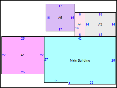
To ensure the synthetic data we generated reflects real-world homes, we collected data from publicly available county datasets. For our pipeline instance, we gathered data from Northampton County, Pennsylvania, where two of the authors work and reside. To collect this data, we implemented a web scraper using Selenium WebDriver \parenciteselenium and ChromeDriver \parencitechromedriver. For each residential property on each street in the list of streets to process, the scraper extracts key attributes, such as number of rooms, total floor area, and other metadata listed in Table 1. This data is saved to a JavaScript Object Notation (JSON)file for each home. Additionally, the scraper downloads two images: a street view photograph and a floor plan, both of which are made available on the County’s public-facing platform. An example of each is depicted in Figure 2.
Although this implementation targets a single county, the pipeline is modular and can be adapted to different public record schemas and regional metadata formats. Currently, our scraper is configured to gather information from Northampton County’s instance of iasWorld. Developed by Tyler Technologies, iasWorld is an Enterprise Assessment & Tax solution used by “jurisdictions in 26 US states, four Canadian provinces, and the Bahamas” \parencitetyler2022orange. However, our implementation could easily be modified to point to another instance, such as in DeKalb County, Georgia.
Moreover, multiple web scraping modules could be employed to gather data from differently structured systems simultaneously. For example, Lancaster County, Pennsylvania uses a tool by Devnet called Edge. To create a dataset consisting of homes in Lancaster, Northampton, and DeKalb county, simply create two versions of the scrapers, one for Devnet and one for iasWorld. While much of the high-level scraping logic would remain consistent across systems, the underlying HTML structure, identifiers, and parsing rules would require tool-specific adjustments. Nevertheless, the modular design of the ingestion pipeline allows these adaptations to be incorporated without changing the overall framework.

| Collected Data | Type |
|---|---|
| Year Built | Year |
| Remodeled Year | Year |
| Land Use Code | String |
| Total Square Feet Living Area | Number |
| Number of Stories | Number |
| Grade | String |
| CDU | String |
| Building Style | String |
| Total Rooms | Number |
| Bedrooms | Number |
| Full Baths | Number |
| Half Baths | Number |
| Additional Fixtures | Number |
| Total Fixtures | Number |
| Heat/Air Cond | String |
| Heating Fuel Type | String |
| Heating System Type | String |
| Attic Code | String |
| Unfinished Area | Number |
| Rec Room Area | Number |
| Finished Basement Area | Number |
| Fireplace Openings | Number |
| Fireplace Stacks | Number |
| Prefab Fireplaces | Number |
| Basement Garage (Number of Cars) | Number |
| Condo Level | Number |
| Condo/Townhouse Type | String |
| Basement | String |
| Exterior Wall Material | String |
| Physical Condition | String |
| Sketch Data | Dictionary of floorplan segment areas |
3.2 Processing Images
After scraping the street view photographs and floor plans from the county portal, they are analyzed using LLaVA \parenciteliuVisualInstructionTuning2023 version 1.5 with 7 billion parameters, distributed on HuggingFace (llava-hf/llava-1.5-7b-hf). This step processes both files to translate them into a textual description. For example, the floor plans can be used to define the geometry of the home, and the image to determine the quality and number of windows. The goal of utilizing the floor plan image is not to generate a one-to-one replication of a given home, but instead, it is used to produce structurally plausible layouts. This allows our pipeline to infer important aspects of the homes that will be used to generate the GeoJSON, which is ultimately used to generate the Input Definition File (IDF)file required by EnergyPlus.
3.2.1 Evaluating Visual Focus with Occlusion Testing
In image processing, it is crucial that only key portions of the images in question trigger differences in the response of a model. For example, if the prompt asks about the state of the roof of a home, the tree next to the home should be inconsequential in comparison to the roof itself. In this document, we refer to this measure as focus. Following, we present an evaluation of focus using occlusion, which is intended to measure differential sensitivity rather than measuring semantic correctness or providing a formal visual attribution method.
Occlusionmeasures the necessity of a part of an image: if removing a feature causes the prediction to change, that feature was necessary for the model’s decision \parencitehookerBenchmarkInterpretabilityMethods2019, balkirNecessitySufficiencyExplaining2022. When we remove image portions, we replace them with a neutral value, such as black. This creates a masked version of the image. The degree of change measured between the model’s output for this masked image and its baseline response reflects the importance of the masked cell. High sensitivity to the removal of a feature suggests the model relied heavily on that region to produce its output, indicating that the region was internally necessary to the model’s decision process.
During the development of our pipeline, we identified two candidate LLMsto employ for image processing. To determine the best model for this task, we compared the focus of the GPTand LLaVALLMswhen analyzing images using occlusion tests. We provided the models with twenty different images of homes: ten with roofs showing no signs of damage, and ten with roofs with significant damage. Each model was instructed to evaluate and describe the state of the roof and justify its evaluation. We first took a baseline where no part of the image was masked. Then, the image was divided into one hundred cells, a number we selected to balance effectiveness, efficiency, and cost. Each cell of the image was masked, and the model was executed on the original prompt and this new image. Textual responses were embedded into vectors using the all-MiniLM-L6-v2 SentenceTransformers model \parencitereimersSentenceBERTSentenceEmbeddings2019, a lightweight and widely used model sufficient for obtaining sentence-level numerical representations. Then, to measure the semantic difference between each execution of the experiment, we took the cosine distance of each embedded response from the baseline. Additionally, heatmaps of these differences were assembled using matplotlib \parencitethematplotlibdevelopmentteamMatplotlibVisualizationPython2025.
We categorize cells as follows: if a cell contains any visible portion of the roof, it is a roof cell; otherwise, it is considered a non-roof cell. This categorization was performed manually for all twenty images. The mean difference value in roof cells and non-roof cells for each image was calculated. Figure 3 depicts the distribution of the forward occlusion results. These scatter plots are particularly telling—GPT(Figure 3(a)) evenly scatters the data points on either side of the line , indicating it has no preference for which area in the image is considered important. In comparison, LLaVA(Figure 3(b)) tends to produce results in the upper half of the graph. These results illustrate that, unlike GPT, LLaVAconsistently exhibits greater sensitivity to roof regions than to non-roof regions, indicating stronger task-relevant visual focus in our occlusion experiments.


Additionally, overall means and standard deviations were calculated for GPTand LLaVA(Figure 4). In a well-focused model, the mean difference in the relevant area should be greater than the mean difference anywhere else. This behavior occurs since relevant cells should account for the majority of the response given by the model. In our experiments, we observe that GPTreports identical roof and non-roof mean differences (Figure 4(a)). However, LLaVAachieved a roof mean difference approximately greater than its non-roof mean difference (Figure 4(b)).
| Mean Difference | SD | |
|---|---|---|
| Roof | 0.0956 | 0.0384 |
| Non-Roof | 0.0956 | 0.0408 |
| Mean Difference | SD | |
|---|---|---|
| Roof | 0.0208 | 0.0241 |
| Non-Roof | 0.0149 | 0.0197 |
Cells were partitioned into roof and non-roof groups within each image. The difference between the mean occlusion effects of the two groups was computed for each image and subsequently averaged across all images to obtain the mean paired difference (MPD). This value is a numerical representation of the relative importance of both cells that depict the roof and those that do not. Thus, the sign of the MPD indicates which cell group produced the larger occlusion effect, while its magnitude reflects the size of the difference. The results are reported in Table 2.
To assess whether the MPD is statistically significant, we employed paired Wilcoxon signed-rank tests due to the small sample size and the non-normal, zero-heavy distribution of the differences. A statistically significant result () indicates that the roof and non-roof mean differences are distinct for the given language model. GPT showed no statistically detectable difference between roof and non-roof regions (), while LLaVA demonstrated significantly greater roof-region sensitivity () with a moderate paired effect size (). Although occluding both roof and non-roof regions altered LLaVA’s responses, the significantly larger occlusion effects observed for roof regions indicate that the model relied more heavily on task-relevant visual information. These statistical findings are summarized in Table 2.
| Model | Mean Paired Difference | Wilcoxon -value | Cohen’s |
|---|---|---|---|
| GPT | |||
| LLaVA |
When we compared our individual GPT and LLaVAocclusion results, we found that LLaVAhas greater roof-region sensitivity. LLaVAis much more particular about which cells are key to construct the response; GPT produces results that look stochastic. Figure 5 displays one noteworthy example—LLaVAfocuses on a more specific section of the image, primarily consisting of the home’s roof. GPT, on the other hand, behaves much more randomly. Each value in the cell is the semantic difference, and the background tint of the cell represents the scaled semantic difference, where the brightest background represents the largest difference and the darkest represents the smallest. In Figure 5(a), the semantic difference is generally larger on the roof than on other parts of the image. A small semantic difference is a signal that a given portion of the image is less important to the model in order while formulating a response. In Figure 5(b), the majority of cells are moderately important to the model in formulating a response—even cells containing walls or grass. Comparing the two, LLaVAdemonstrates better focus on the more important parts of the image. Full occlusion experimental details, hypotheses, and findings are available in A.
The goal of the occlusion experiments was not to evaluate the quality of the image-to-text translation, as this aspect has been examined extensively in prior work by the model’s developers \parenciteliuVisualInstructionTuning2023, liuImprovedBaselinesVisual2024. Those studies report strong performance on image description tasks, motivating our use of LLaVA as the image description component of the pipeline.


3.3 Generating GeoJSON
Once the images are processed, we utilize the descriptions given by LLaVAin a GPTprompt, available in B, to generate a GeoJSONfile and home inspection notes. The prompt provides the image descriptions (Section 3.2) and data that was scraped from the county portal (Section 3.1) and directs the model to take two actions:
-
•
The prompt instructs GPTto generate a GeoJSONfile for the building, including geometry, data from the county, and five estimated performance parameters. These estimated parameters, defined according to standard convention, include the HVAC heating and cooling coefficients of performance and R-values for the roof and wall.
-
•
The prompt directs GPTto write a short inspection note, focused on energy-related observations such as insulation, HVAC type/age, visible windows, and any inferred upgrades. This inspection note is placed in the GeoJSONfile.
The prompt contains strict guidelines intended to improve output validity, completeness, and simulation-oriented realism. In the pipeline, generated building footprints are additionally constrained using metadata-derived target footprint area estimates based on the reported living area and number of stories for each home. The prompt explicitly instructs GPTto generate compact residential-scale geometries whose footprint approximately matches the target estimate derived from the metadata. After generation, the area of the resulting geometry is validated against the reported footprint area. Given that most footprints are characteristically rectangular, we validate accuracy of the generated home by comparing the area of the generated footprint with the reported values.
If the area of the generated footprint falls outside the acceptable scale range, defined in our experiments as between and the true square footage of the home, the pipeline automatically reprompts GPTwith corrective feedback regarding the size of the generated geometry. When more than six generation attempts fail to satisfy this constraint, a deterministic scaling correction is applied to improve footprint consistency while preserving the overall building shape. Table 3 shows the number of generation attempts required for each home. Of the 247 generated homes, 116 (47.0%) satisfied the geometric constraint on the initial generation. The remaining 131 homes required at least one regeneration, with progressively fewer requiring additional attempts. Only two homes (0.8%) exhausted all six generation attempts and required deterministic scaling.
| Generation Attempts | Homes | Percent | Cumulative Homes |
|---|---|---|---|
| 1 (accepted immediately) | 117 | 47.4% | 117 |
| 2 | 70 | 28.3% | 187 |
| 3 | 35 | 14.2% | 222 |
| 4 | 14 | 5.7% | 236 |
| 5 | 6 | 2.4% | 242 |
| 6 | 3 | 1.2% | 245 |
| Deterministic scaling | 2 | 0.8% | 247 |
| Total | 247 | 100.0% | 247 |
To evaluate scale consistency between the synthetic homes and the original residential metadata, we compared generated footprint areas against county-derived target footprint estimates computed from the reported living area and number of stories for each home. Generated footprint areas exhibited a statistically significant positive correlation with these metadata-derived target areas ().
While the previous analysis evaluates the plausibility of the area of the generated homes, it does not address the reliability of the underlying structured-data generation process. We use GPTfor structured data generation given its strong ability to produce well-formed JSONoutputs from descriptive prompts. Prior work has demonstrated that LLMscan reliably generate outputs that conform to predefined schemas under strict schema constraints, even with no previous prompting or task-specific fine tuning. For example, the StructuredRAG benchmark suite showed format compliance under JSONprompt conditions \parenciteshortenStructuredRAGJSONResponse2024.
As we built the pipeline, we reviewed GPT’s responses and found that it seldom failed to adhere to the expected JSONstructure. In the rare case that malformed output is produced, the pipeline catches the parsing error and automatically reprompts GPT. Only one synthetic home failed generation, of the attempted homes. An excerpt from an example GeoJSONobject is provided in Figure 6.
3.4 Running EnergyPlus Simulations
To execute a simulation in EnergyPlus, we take the GeoJSONgenerated by GPT(Section 3.3) and convert it to an IDFfile for use in EnergyPlus. We use a template IDFfile, filled with default values that are replaced with variables from the GeoJSONdata, such as the geometry, HVAC heating and cooling coefficients of performance and R-values for the wall and roof. Additionally, the template has many fields with constant values, such as the simulation running period and materials, constructions, and zones used in the simulation. Once the details from the GeoJSONare copied into the template, a final IDFfile is produced.
The templating process is facilitated with the eppy package \parencitesantoshphilipEppy2024, which makes programmatic IDFgeneration straightforward. Then, we use ExpandObjects to prepare the file for simulation. ExpandObjects is bundled with EnergyPlus, and its primary use case is to take an IDFand expand template objects—such as the HVACTemplate we use—into full systems \parenciteexpandobjects2023. Finally, we run the expanded IDFfile through EnergyPlus, producing final simulation results.
We write the inspection notes and EnergyPlus simulation results for each example into one JSON Lines (JSONL)file. This completes our end-to-end dataset generation process, yielding a unified dataset that combines textual and simulation-based information.
4 Validating Plausibility of Pipeline Generated Data
Following prior work on synthetic data evaluation \parencitepatkiSyntheticDataVault2016, goncalvesGenerationEvaluationSynthetic2020, duSystematicAssessmentTabular2025, lautrup2024syntheval, we view synthetic data plausibility as application dependent, linked to the properties of the domain in focus rather than as a single universal mechanism to validate data across all domains. Given that the purpose of our framework is to generate simulation-ready residential building models and in this field there is not an agreed validation approach for such synthetic data, we utilize interval coverage metrics to evaluate the empirical plausibility of our generated data.
Interval coverage metrics are widely used to evaluate whether model outputs remain within statistically expected ranges \parencitekrugerPredictionIntervalsEconomic2024,Schmidinger2023. \textcitekrugerPredictionIntervalsEconomic2024 use interval coverage as a principal measure of interval calibration, whereas \textciteSchmidinger2023 evaluate coverage alongside complementary uncertainty metrics. Furthermore, percentile distributions have been used as part of the evaluation of synthetic building-energy profiles \parencitePatidar2016. Drawing on these complementary evaluation perspectives, we define plausible reference intervals of the corresponding ResStock \parenciteResStock2024_1Dataset, ResStockTechRefV3_3_0 variables and evaluate the proportion of generated values that fall within these intervals. ResStock is a publicly available dataset developed by the U.S. Department of Energy to represent the U.S. residential building stock. The selected interval, the 10th–90th percentiles, excludes the extreme tails of the empirical ResStock distribution while retaining its central region. The bottom of the interval was selected given that \textcitePatidar2016 leave the 0th-10th percentiles out of their evaluation interval, and the top was selected for symmetry.
Our comparison is restricted to Climate Zone 4A and to the four variables that vary across synthetic homes—Wall R-Value, Roof R-Value, Cooling COP, and Heating COP—because of their importance in building energy simulation. Each variable is evaluated separately against its corresponding ResStock reference interval. This reflects the objective of assessing the plausibility of individual generated building characteristics, including uncommon but physically plausible homes that need not conform to the joint distribution of the reference dataset. The remaining approximately 150 variables are fixed template values outside the generative pipeline, although the pipeline could readily be extended to generate these as well. The evaluation corpus consists of 247 synthetic homes and 2,000 ResStock Climate Zone 4A samples. In addition to the proposed plausibility coverage metric, we report statistics that provide descriptive context for both datasets.
Table 4 reports the plausibility coverage results for the four variables across all synthetic homes by displaying the percentage of values that fall within the ResStock 10th–90th percentile interval. We observed coverage greater than for all variables and greater than for three of the four variables. Under our coverage-based definition of plausibility, these results suggest that the generated values for these variables are largely consistent with the typical ranges observed in the reference dataset. Additionally, the table reports summary statistics for both datasets, including the mean and median of each variable for the synthetic homes and the interquartile range (IQR) observed in ResStock. These statistics are provided for descriptive context and are not used when computing the plausibility coverage metric.
| Variable | Coverage (%) | ResStock Q1–Q3 | Synthetic Mean | Synthetic Median |
|---|---|---|---|---|
| Wall R-Value | 98.38 | 1.94–2.64 | 2.42 | 2.29 |
| Roof R-Value | 100.0 | 3.35–6.69 | 5.21 | 5.28 |
| Cooling COP | 58.70 | 3.1–3.8 | 2.90 | 3.00 |
| Heating COP | 99.59 | 0.8–1.0 | 0.82 | 0.85 |
Compared to prior generative urban-energy workflows, our framework incorporates both multimodal sensitivity analysis and reference-based plausibility validation against a national reference dataset. Occlusion provides empirical evidence that the image processing component of the pipeline behaves as intended. We additionally show that the generated variables generally fall within the empirically plausible reference intervals derived from ResStock, with coverage exceeding 95% for three of the four evaluated variables. While concerns regarding hallucinations and reliability remain important when using LLMs, the results presented here indicate that the proposed safeguards and validation procedures help mitigate some of the issues identified by \textciteliuLargeLanguageModels2025.
5 Conclusion
In this work, we presented a multimodal framework for generating simulation-ready synthetic residential data from public records, imagery by applying generative AI models. The results demonstrate the feasibility of generating simulation-ready synthetic residential data when comprehensive real-world data are unavailable. To the best of our knowledge, no prior approach has combined these heterogeneous data sources into a unified pipeline capable of producing both structured simulation inputs and complementary textual descriptions for residential buildings.
The proposed pipeline produces both structured building-energy models and accompanying textual descriptions, enabling the creation of dual-modality datasets suitable for simulation and downstream machine learning applications. To evaluate the reliability of the generated outputs, we introduced a validation framework that combines multimodal sensitivity analysis, structured-output verification, and plausibility-oriented comparison against a national reference dataset. Together, these analyses provide evidence that the generated homes are physically plausible, simulation compatible, and aligned with the intended objectives of the pipeline.
Recent reviews have highlighted the growing relevance of generative AI in building energy research while also identifying challenges related to reliability, validation, and practical deployment, motivating the development of robust methods for energy simulation workflows \parencitexuLeveragingGenerativeAI2024, liuLargeLanguageModels2025. The framework presented in this work contributes to this emerging area by providing a flexible approach for generating simulation-ready residential data under conditions of limited data availability. Beyond its use for synthetic home generation, the framework may support a variety of downstream applications and can be extended in several directions. One particularly promising avenue for future work is the use of the generated data to support the training of machine learning models for urban energy applications. For instance, the pipeline could be expanded to utilize the resulting simulation data and inspection notes to label the efficiency of particular components that affect the energy efficiency of a home. These labeled homes could be used to train an MLmodel that provide recommendations for energy efficiency retrofits. Furthermore, such a model could help prioritize retrofit interventions for residential buildings. Moreover, such downstream use would complement the validation presented in this work by displaying the dataset’s usefulness for predictive modeling.
Overall, this work evaluates plausibility, simulation compatibility, and task-aligned multimodal sensitivity, which align with the intended use of the generated homes as simulation-ready synthetic residential data. Rather than reconstructing ground-truth building geometries or calibrated utility measurements, the pipeline is designed to produce physically plausible and operationally useful representations under conditions of limited real-world data availability. Constructing large-scale authoritative datasets that satisfy realism constraints remains a broader challenge in residential energy modeling and synthetic urban data generation.
Ultimately, the high cost, limited availability, and privacy concerns associated with collecting urban energy data motivate the use of synthetic alternatives. Our framework helps address these data-access challenges by producing simulation-ready synthetic data accompanied by plausibility-oriented validation. By reducing dependence on costly or restricted data sources, the approach will broaden access to data-driven research in the urban energy domain.
Acknowledgments
The authors extend gratitude to Lafayette College for supporting this work by funding it through the EXCEL Scholars program and providing computational resources with the Firebird high performance computing cluster. Access to the JetStream2 system was made possible via the NSF-funded ACCESS program, facilitated by Lafayette College. We also thank the NSF and ACCESS for supporting this resource, and Indiana University for hosting JetStream2 as a part of the ACCESS program.
CRediT Author Attributions
Jackson Eshbaugh: Software, Investigation, Writing - Original Draft, Visualization, Validation, Data Curation. Chetan Tiwari: Conceptualization, Writing - Review and Editing, Supervision (supporting). Jorge Silveyra: Conceptualization, Writing - Review and Editing, Methodology, Supervision (lead), Project Administration, Validation
Glossary
Appendix A Occlusion Results
In this appendix, we provide detailed information and results from our occlusion tests. Firstly, when running the test we utilized identical prompts for each model. For GPT, we prompted:
You are a certified home inspector. Describe the status roof. Is it in good condition? Why or why not?
Likewise, we prompted LLaVA with the following:
USER: <image>
You are a certified home inspector. Describe the status roof. Is it in good condition? Why or why not? ASSISTANT:
These prompts differ slightly due to how the models are trained; namely, LLaVA expects an image token and labeled portions of the message. The majority of LLMs behave this way, and the GPT API likely wraps the given prompt in something similar.
Next, we provide our hypotheses pertaining to the performance of both models. We hypothesize that LLaVA’s advantage stems from its architecture: it employs an early fusion design in which images are converted into visual tokens by CLIP \parenciteradfordLearningTransferableVisual2021 that are then prepended to the textual prompt \parenciteliuVisualInstructionTuning2023. These visual tokens are passed through the transformer layers of the LLMtogether with text tokens, enabling multimodal attention at every layer. It has been demonstrated that vision tokens are most critical for a model in early layers, when they fuse into text tokens \parencitezhangLLaVAMiniEfficientImage2025. A likely result of this is the reduction of the model’s sensitivity to variations in the image, which may explain its stronger performance in our experiments.
While GPT-4V (GPT’s vision model) is proprietary, the case can be made that it possesses a different structure. Evaluation studies show that it performs well across visual reasoning and captioning tasks, but it falls short in fine grained visual problems, requiring complex visual tasks to be broken up into interleaved subfigures and text \parenciteyangDawnLMMsPreliminary2023. These evaluations are similar to evaluations from late fusion (connector) models. For example, BLIP-2 shows strengths in captioning images and instruction-following, while it is less robust with fine-grained spatial reasoning \parenciteliBLIP2BootstrappingLanguageImage2023. Another model, MiniGPT-4, demonstrates a similar profile: it has strengths in tasks such as image description, but falters with complex spatial reasoning \parencitezhuMiniGPT4EnhancingVisionLanguage2023. Both BLIP-2 and MiniGPT-4 are late fusion models, where compressed visual features are routed into the LLMat later stages \parenciteliBLIP2BootstrappingLanguageImage2023, zhuMiniGPT4EnhancingVisionLanguage2023. As shown, BLIP-2, MiniGPT-4, and GPT-4V all suffer from a very similar weakness: fine-grained or complex spatial reasoning. Based on this similarity, we hypothesize that GPT-4V is also a late fusion model. This helps explain why GPTperformed differently from LLaVAin our experiments: as structure dictates function, differences in behavior strongly suggest differences in design. On the basis of this analysis, we feel confident to select LLaVAto complete this task.
In Table 5, we provide our forward occlusion results, including roof mean difference (RMD) and non-roof mean difference (NRMD) values from both GPT and LLaVA and references to figures displaying GPT and LLaVA heatmaps side by side.
| Metric | 1 | 2 | 3 | 4 | 5 | 6 | 7 | 8 | 9 | 10 |
|---|---|---|---|---|---|---|---|---|---|---|
| Damaged Roofs | ||||||||||
| GPT RMD | 0.0856 | 0.0920 | 0.0730 | 0.0689 | 0.1127 | 0.0453 | 0.0516 | 0.0603 | 0.1149 | 0.0419 |
| GPT NRMD | 0.0903 | 0.0745 | 0.0615 | 0.0824 | 0.0900 | 0.0375 | 0.0485 | 0.0900 | 0.1000 | 0.0442 |
| LLaVA RMD | 0.0033 | 0.0324 | 0.0949 | 0.0093 | 0.0262 | 0.0269 | 0.0356 | 0.0055 | 0.0038 | 0.0208 |
| LLaVA NRMD | 0.0057 | 0.0545 | 0.0723 | 0.0059 | 0.0200 | 0.0000 | 0.0335 | 0.0055 | 0.0022 | 0.0042 |
| Roof Cells | 70 | 80 | 53 | 83 | 97 | 96 | 80 | 96 | 91 | 88 |
| Non-Roof Cells | 30 | 20 | 47 | 17 | 3 | 4 | 20 | 4 | 9 | 12 |
| Figure | 7 | 8 | 9 | 10 | 11 | 12 | 13 | 14 | 15 | 16 |
| Undamaged Roofs | ||||||||||
| GPT RMD | 0.1128 | 0.0785 | 0.1465 | 0.1508 | 0.0822 | 0.0956 | 0.1087 | 0.2005 | 0.0696 | 0.1200 |
| GPT NRMD | 0.1055 | 0.0742 | 0.1872 | 0.1598 | 0.0884 | 0.0930 | 0.1230 | 0.1898 | 0.0768 | 0.0959 |
| LLaVA RMD | 0.0709 | 0.0085 | 0.0007 | 0.0000 | 0.0340 | 0.0108 | 0.0066 | 0.0000 | 0.0017 | 0.0240 |
| LLaVA NRMD | 0.0313 | 0.0062 | 0.0000 | 0.0000 | 0.0321 | 0.0023 | 0.0030 | 0.0000 | 0.0015 | 0.0181 |
| Roof Cells | 53 | 47 | 68 | 49 | 81 | 39 | 70 | 60 | 47 | 73 |
| Non-Roof Cells | 47 | 53 | 32 | 51 | 19 | 61 | 30 | 40 | 53 | 27 |
| Figure | 17 | 18 | 19 | 20 | 21 | 22 | 23 | 24 | 25 | 26 |


Appendix B GeoJSON Generation Prompt
In this appendix, we provide the prompts used to generate the GeoJSON data in Section 3.3. First, we list the main prompt, then the retry prompt for unreasonable geometry.