Primordial black holes versus their impersonators at gravitational wave observatories
Abstract
The detection of primordial black holes (PBHs) would mark a major breakthrough, with far-reaching implications for early universe cosmology, fundamental physics, and the nature of dark matter. Gravitational wave observations have recently emerged as a powerful tool to test the existence and properties of PBHs, as these objects leave distinctive imprints on the gravitational waveform. Notably, there are no known astrophysical processes that can form sub-solar mass black holes, making their discovery a compelling signal of new physics. In addition to PBHs, we consider other exotic compact object (ECO) candidates—such as strange quark stars and boson stars—which can produce similar gravitational signatures and potentially mimic PBHs. In this work, we employ the Fisher matrix formalism to explore a broad parameter space, including binary masses, spins, and different nuclear and quark matter equations of state. Our goal is to assess the ability of next-generation gravitational wave detectors—specifically Cosmic Explorer and the Einstein Telescope—to distinguish PBHs from ECOs, stellar BHs and neutron stars. We compute the maximum luminosity distances (LDs) at which confident () detections of sub-solar masses or tidal effects are possible, providing quantitative benchmarks for PBH identification or exclusion under various observational scenarios. Our results indicate that next-generation detectors will be capable of probing sub-solar mass PBHs out to cosmological distances of . For heavier objects with masses up to , we show that PBHs can be distinguished from neutron stars via their lack of tidal effects up to redshifts of .
1 Introduction
The discovery of new classes of compact objects beyond the standard astrophysical paradigm would offer profound insights into early-universe cosmology and the nature of dark matter. Among the most intriguing candidates are primordial black holes [19, 49] and exotic compact objects [45], such as strange quark stars (SQSs) [92, 72] or boson stars [25, 93], which could exist in mass regimes inaccessible to standard stellar evolution [26, 33, 27]. In particular, the detection of a sub-solar mass compact object would serve as a compelling signature of new physics, since no known astrophysical process is expected to produce black holes or neutron stars (NSs) below the Chandrasekhar limit. Recent searches within the LIGO-Virgo-KAGRA (LVK) data have already begun placing stringent constraints on such populations. The observation of gravitational waves (GWs) from compact binary mergers provides a unique avenue for probing these objects [65, 90, 6, 4].
To distinguish between various sub-solar candidates, one must identify the distinct imprints they leave on the GW signal. A central role is played by the tidal deformability, characterized by the quadrupolar Love number and the dimensionless parameter
| (1.1) |
which encodes the internal structure and composition of the companions during the late inspiral phase [72, 13, 30], for a body of radius and mass .
An especially interesting regime is that of sub-TOV masses, where the object mass falls below the maximum mass supported by the neutron-star Tolman-Oppenheimer-Volkoff (TOV) limit. For material objects in this regime (NSs, SQSs, or BSs), the compactness is relatively low and the tidal deformability can be large [72, 70]. By contrast, PBHs are vacuum solutions of GR and have strictly vanishing tidal deformability, and in classical GR [13, 47, 33]. The detection of a sub-solar-mass black hole with would thus strongly indicate a primordial origin, whereas a sub-solar-mass compact object with would point to a material configuration (NS or ECO) [26, 27, 82].
From a waveform modeling perspective, tidal contributions enter the GW phase at post-Newtonian (PN) order and predominantly affect the late inspiral. Their impact is enhanced for low-mass, low-compactness objects, but remains challenging to measure even with third-generation (3G) detectors, owing to the high PN order and correlations with other parameters [89, 72, 26]. Accurate modeling of tidal terms is therefore crucial to avoid biases in inferred masses, radii, and object classification [89, 43, 22, 27].
Upcoming observing runs of LIGO–Virgo–KAGRA and, in particular, future 3G observatories such as Cosmic Explorer (CE) [38, 77] and the Einstein Telescope (ET) [76, 62] will dramatically improve sensitivity to both sub-solar-mass systems and tidal signatures [67, 1]. This raises a concrete question: to what redshift can 3G detectors identify sub-solar-mass compact objects, and within what distance can they distinguish PBHs from material counterparts via tidal effects? Answering these questions requires combining realistic assumptions about detector networks and waveform models with physically motivated mass and tidal-deformability ranges for NSs, SQSs, BSs, and PBHs.
In this work we address this problem using the GWJulia code [9] and the Fisher information matrix (FIM) formalism [40, 29, 88]. The FIM has been widely used for GW forecasts, including for 3G detectors [79, 52, 36, 16, 15, 34, 60, 1], and provides reliable estimates in the high-SNR regime [36, 9]. We use it here to quantify: (i) the mass-based identification horizon for sub-solar companions, and (ii) the tidal-discrimination horizon at which PBHs and other ECOs can be distinguished from standard NSs.
The paper is organized as follows. In Sec. 2 we define our Fisher-matrix setup and the criterion for mass-based sub-solar identification. In Sec. 3 we summarize the compact-object models considered in this work, i.e., NSs, SQSs, BSs, and PBHs, focusing on their expected mass ranges and tidal deformabilities. Section 4 details the detector network, waveform choices, and EOS models. The main results are presented in Sec. 5, and we conclude in Sec. 6.
2 Maximum luminosity distance
Our first goal is to quantify, for a given compact-binary configuration in which one object is sub-solar, the maximum luminosity distance at which the mass of the sub-solar companion can be identified at the level. We do so using the Fisher information matrix, defined as [40, 29, 88]
| (2.1) |
where is the log-likelihood of the data stream given parameters , and the average is taken over noise realizations, see, appendix˜A for more details on the formalism. The parameter vector includes intrinsic and extrinsic quantities,
| (2.2) |
where is the chirp mass at detector, the mass ratio, the dimensionless component spins, the luminosity distance, the sky position, the inclination, the polarization angle, and , the time and phase at coalescence. For material objects (NSs or ECOs), denote the tidal deformabilities; for PBHs we set . In this work we will consider non-precessing waveforms, therefore .
In the high-SNR regime, the likelihood of the event , converges to a Gaussian. Therefore, the covariance matrix of parameter estimates is approximated by , and, for instance, the uncertainty on the mass ratio is given by [88].
Since we want to obtain contraints on the lighter companion in the merger we need to perform a conversion of the FIM. The conversion is , which is performed assuming a cosmology, Planck-18 [7] in our case. This is needed because the chirp mass at the source is linked to the chirp mass measured at the detector with
| (2.3) |
This, united with the definition of chirp mass at the source, allows us to perform the change of variables in the FIM. Our primary diagnostic for sub-solar identification is the luminosity distance satisfying
| (2.4) |
therefore, we define as the maximum luminosity distance at which a sub-solar mass object can be confidently identified at the level. Our primary objective is to analyze how different configurations of intrinsic parameters (masses, spins, and EOS-dependent tidal deformabilities ) impact this detection horizon. However, the extrinsic parameters can significantly influence the estimation of . Ideally, one would marginalize the results over these variables to isolate the effects of the intrinsic physics; however, a full marginalization procedure is computationally prohibitive. To balance physical rigor with computational feasibility, we adopt a sampling approach: for each unique intrinsic configuration, we generate a catalog of 20 binaries with extrinsic parameters drawn from their respective astrophysical priors [5, 9]. This allows us to provide results that are representative of the expected observational population while remaining within manageable numerical limits. Then, for each of the 20 realizations identified with parameters , we determine, via a bisection search on , the maximum LD , using Eq. (2.4). We then take the median over this catalog as our measure of the maximum LD (or equivalently, redshift) of that intrinsic configuration. This median-based approach has several advantages. It averages over the strong variation in network response with sky position and the binary inclination and it yields a more robust measure. Moreover, it alleviates possible shortcomings of the FIM framework, as we discuss later.
In addition to mass-based identification, we also use the FIM to forecast the precision on tidal parameters and to determine the maximum redshift at which nonzero can be measured with significance, thereby excluding the PBH (or other ECO) hypothesis. The same catalog-based procedure is used, but with the relevant criterion applied to , as detailed in Sec. 5.
While the FIM is a powerful tool, its convergence to the true posterior distribution is subject to several important caveats. GW likelihoods are frequently multimodal and can exhibit significant non-Gaussian tails, even at high SNRs. Parameters such as spins and tidal deformabilities are particularly susceptible to this behavior. For instance, low sensitivity to spin can cause the FIM to predict errors that exceed physical boundaries (e.g., ). While some effects can be mitigated by enforcing prior bounds, such as the approach in [37], others, like the strong degeneracy between individual tidal deformabilities, remain inherently non-Gaussian. Numerical stability also poses a significant hurdle. Inverting the FIM can be ill-conditioned, a problem exacerbated by the additional parameters introduced in tidal models [88]. Similarly, face-on events produce nearly circular polarization, inducing near-total degeneracies between inclination, distance, phase, and polarization angle. Because the inversion process is sensitive to even a single poorly constrained parameter, a nearly singular matrix (characterized by near-zero eigenvalues) can lead to significant numerical errors. Despite these limitations, the FIM remains a standard when analyzing large event populations, e.g., [1]. Although individual low-SNR or degenerate events may yield biased results, the collective parameters inferred from a large catalog tend to converge toward the true distribution obtained via full Bayesian estimation [10].
3 Compact-object models and tidal properties
In this section we summarize the compact-object families considered in our analysis and the aspects that are directly relevant for our Fisher forecasts. Our goal is to identify the characteristic mass ranges, compactness, and tidal deformabilities that determine how easily different objects can mimic or be distinguished from primordial black holes in 3G observations.
We consider four representative classes: (i) neutron stars modeled with the AP3 EOS, (ii) strange quark stars described by a self-bound quark-matter EOS, (iii) phenomenological boson stars whose tidal deformability is enhanced relative to AP3, and (iv) primordial black holes, which provide a null hypothesis with . For the material objects (NSs, SQSs, BSs), the key quantities are the allowed mass range and the mass– relation; for PBHs, the crucial features are the absence of tidal deformability and the freedom to populate the sub-solar mass range.
3.1 Strange quark stars
Strange quark stars are hypothetical compact stars composed of deconfined up, down, and strange quarks, motivated by the Bodmer–Witten hypothesis that strange quark matter may represent the true ground state of hadronic matter [92, 14]. Their macroscopic properties are governed by the EOS of strange quark matter, which determines the mass–radius relation and thus the tidal deformability.
For our purposes, the key aspects of SQSs are:
-
•
Mass range. For viable EOSs compatible with massive pulsars such as PSR J0740+6620 () [28], SQSs can reach maximum masses , similar to neutron stars. Unlike NSs, however, self-bound SQS configurations can in principle extend to significantly lower masses, potentially well below for sufficiently small bag constants or appropriate microphysics (see, e.g., [94, 11]).
-
•
Tidal deformability. For a given mass, SQSs are typically more compact than NSs and therefore have smaller tidal deformabilities . Representative models yield values spanning from to several –, depending on the bag constant, color-superconducting gap, and additional QCD corrections [95, 64]. This implies that, in the sub-TOV mass regime, SQSs can still exhibit sizable tidal signatures, but generically somewhat smaller than those of NSs at the same mass.
In our analysis we do not attempt to resolve the full microphysical parameter space of SQS EOSs. Instead, we adopt a representative SQS model, denoted SQM3 [74], that is consistent with current mass and tidal constraints and yields a mass– relation intermediate between soft and stiff hadronic EOSs. This choice captures the qualitative behavior of SQS tidal deformabilities in the sub-TOV regime and allows us to assess how easily SQSs could mimic PBHs in 3G observations.
Spin properties of SQSs are less critical for our purposes. Existing modeling indicates that rapidly rotating SQSs with – are possible for realistic EOSs before reaching the mass-shedding limit [12]. In the present work, spins enter only through the adopted spin ranges in our waveform modeling, as summarized in Sec. 4.
3.2 Boson stars
Boson stars are self-gravitating configurations of complex scalar or vector fields that are stabilized by the balance between gravity and the field’s gradient and self-interaction energies [93, 81]. They provide a well-studied example of horizonless ECOs that can mimic black holes or neutron stars in mass and compactness, but with distinct tidal properties.
The aspects of BSs that are directly relevant to our analysis are:
- •
-
•
Compactness and tidal deformability. Depending on and the self-interaction potential, BSs can range from relatively diffuse to highly compact. In general, lighter bosons and strong self-interactions favor more extended configurations with large tidal deformabilities , whereas heavier bosons or certain solitonic potentials can produce very compact BSs with much smaller [23, 56].
Given this diversity, a fully microphysical exploration of BS parameter space would be far beyond the scope of this work. Instead, we adopt a phenomenological BS model, denoted BS5, whose mass– relation is chosen to follow that of the AP3 EOS but with tidal deformabilities enhanced by a fixed factor (see Sec. 4 and appendix˜A). This setup is deliberately optimistic: it maximizes the tidal imprint relative to NSs and PBHs, and thus provides an optimistic estimate of how easily BSs could be distinguished from PBHs with 3G detectors.
We do not model BS-specific merger or ringdown effects; instead, we treat BSs as material objects characterized by an effective tidal deformability entering the inspiral waveform.
3.3 Lower mass limits of neutron stars
Neutron stars are formed from the gravitational collapse of massive stellar cores and are stabilized by neutron degeneracy pressure and strong interactions. For our purposes, the key question is how low in mass a stable NS can be, and what tidal deformabilities are expected in the low-mass regime relevant for sub-solar or sub-TOV systems.
Solutions of the TOV equations indicate that the absolute lower mass limit for cold, stable NS configurations is of order – for realistic EOSs [59, 58]. However, proto-NS evolution and supernova dynamics imply that NSs produced in nature are unlikely to populate the very low-mass tail: the minimum formation mass is typically at or above due to thermal pressure and trapped neutrinos in the proto-NS phase [59]. Observationally, well-measured NS masses lie predominantly in the – range.
At fixed EOS, low-mass NSs are less compact and thus exhibit large tidal deformabilities. For the AP3 EOS adopted in our analysis, reaches values of order for and decreases as the mass approaches the TOV maximum (see appendix˜A). This strong mass dependence underlies the key idea of our tidal discrimination forecasts: even modest fractional errors on at low mass translate into powerful constraints on whether a sub-solar (or near-sub-solar) object can be consistent with a material NS.
3.4 Primordial black holes
Primordial black holes are black holes formed in the early Universe from the collapse of large density perturbations or other non-stellar processes such as phase transitions or cosmic-string collapse [20, 46]. Because their masses are set by horizon-scale physics rather than stellar evolution, PBHs can populate a wide mass spectrum, including the sub-solar regime inaccessible to standard astrophysical formation channels (e.g. [49, 19, 21]).
For this work, the relevant PBH properties are [41]:
- •
-
•
Tidal deformability. Classical GR predicts that non-spinning black holes have exactly vanishing tidal Love numbers, and hence [13, 31, 71]. This holds also for Kerr black holes at the PN level relevant for inspiral. As a result, PBHs provide a clean null hypothesis for tidal effects: any robust detection of nonzero for a sub-solar object would strongly disfavor a PBH interpretation.
PBH spins are more model dependent. PBHs forming during radiation domination are expected to have low spins due to the near-sphericity of the initial perturbations [24], whereas formation in matter-dominated eras or subsequent accretion can generate higher spins [48, 32]. In our forecasts, spins enter only through the assumed spin ranges in the waveform models; we do not attempt to constrain detailed spin distributions.
4 Methods and Assumptions
The results are significantly dependent on the network of detectors considered. In this work, we consider a standard 3G network composed of 10 km arm-length triangular ET in Sardinia, plus two CE, one of 40 km arm-length in the US and one of 20 km arm-length also in the US. For more information on the detectors, see appendix˜A. One of the improvements that the FIM analysis can bring is that we do not have to limit the analysis to a few sources, as described in section˜2. Therefore, in each cell of the figures shown, we plot the median maximum redshift calculated from a small catalog of 20 sources. These catalogs, obtained by uniformly sampling the extrinsic parameters (i.e., inclination, sky position, polarization angle, and phase and time of coalescence), were created to partially reduce the noise associated with a single realization and to obtain a more robust result, see section˜2. For each event, we obtain an estimate of the maximum redshift for a detection using a bisection method; subsequently, we take the median of the 20 redshift estimates. This leads to FIM evaluation per plot. The code used for the evaluation is GWJulia [9], which enabled a very fast evaluation of the FIMs, making it feasible to run all the FIMs required for this work on a laptop.
We now proceed with setting up the Fisher Matrix evaluation, and an important question in each scenario is the waveform choice. We use the most advanced waveform at our disposal, given the physical constraints, since the computation time is not a significant issue for FIM analysis111GWJulia has also the possibility of adding higher order harmonics for the binary BH (BBH) case [44]; we reserve the option to add this in future work.. In this work, we analyze different scenarios and summarize the information on the waveforms in table˜1 and in table˜2. For each waveform, in the GWJulia implementation, we use settings replicating the default options of LALSuite [61], e.g., the frequency where to cut the waveform. The waveforms used in this work are IMRPhenomXAS [75] for the BBH case, IMRPhenomD_NRTidal_v2 [51, 55, 35] for the binary NS (BNS) case, IMRPhenomNSBH [69, 87] for the NSBH case, and TaylorF2 [68, 17, 18] when working outside the calibration ranges of the previous waveforms.
The tidal deformability used for NS is obtained using the AP3 EOS [8], with the TOV solver provided by LALSuite [61]. This EOS is compatible with the current constraints, in particular the one provided by GW170817 [3, 67]. The EOS used for SQSs is the SQM3 [74]. For the BS tidal deformability, we consider a phenomenological approach, i.e., for each mass we do not fix the boson mass . Instead, we consider a BS which is softer than a NS, choosing the tidal deformability to follow the AP3 EOS slope but with a five times larger magnitude. This allows us to place more competitive bounds on the tidal deformability of BS, since softer BS will have an even larger signature, without the need to focus on a single boson mass, or potential shape. For more information on the EOS used in this work, we refer to appendix˜A.
| object 1/ object 2 | PBH | NS | ECO |
|---|---|---|---|
| NS | TaylorF2 | IMRPhenomD_Tidal | TaylorF2 |
| BH | IMRPhenomXAS | IMRPhenomNSBH | TaylorF2 |
| ECO | / | / | TaylorF2 |
| waveform | |||||
|---|---|---|---|---|---|
| IMRPhenomD_NRTidal_v2 | [1,3] | [1,3] | [-0.6,0.6] | [-0.6,0.6] | [0,5000] |
| IMRPhenomXAS | [1, 1000] | BBH | [-0.9,0.9] | [-0.9,0.9] | 0. |
| IMRPhenomNSBH | [1,15] | [1,3] | [-0.5,0.5] | 0. | [0,5000] |
5 Results
In fig.˜1, we show the maximum redshift at which a measure of a sub-solar mass PBH is possible in a merger with a neutron star (NS) of varying masses. Therefore we show the redshift such that
| (5.1) |
The waveform used is TaylorF2, which includes leading-order tidal effects but lacks merger and ringdown information—resulting in a conservative estimate of the sensitivity. This choice is made because none of the full inspiral-merger-ringdown waveforms respects physical constraints, i.e., the more massive body is a NS and the secondary body is a BH. The panels depict three spin configurations: low spins, high spin of the PBH and high aligned spins of both bodies. Spins have a modest impact on the inspiral phase, so we find very weak modifications in the different configurations. The optimal configuration is reached for and , with the median horizon redshift extending beyond . This highlights the importance of heavy neutron star companions in maximizing the reach of PBH identification.

In fig.˜2, we consider instead mergers of a sub-solar mass PBH with a stellar black hole companion and we still examine 3 sub-solar detection. This time, we use the IMRPhenomXAS waveform that allows us to account for high mass ratios. Three spin configurations are again analyzed, showing a more pronounced effect from the high spins alignment compared to the NS case, due to the inclusion of the merger in the evaluation. The maximum redshift is attained for BH mass and PBH masses around , reaching beyond . The left panel (low spins) shows the lowest redshift contours, while the right panel (high aligned spins) demonstrates the highest detection reach. The dashed contour denotes the threshold beyond which the mass ratio . The choice of such a threshold is strongly dependent on the goals of the analysis. E.g., in the context of Bayesian parameter estimations, similar thresholds are put in place; however, this choice is a complex topic, dependent on the waveform model, the spins, and total mass of the event [78, 42, 57, 66]. In this work, we consider events inside the full calibration range of IMRPhenomXAS [75]. Beyond , shown in white, the waveform lies outside the calibration range. This plot confirms that high-mass, high-spin BH companions enable the deepest reach for sub-solar PBHs.


Fig. 3 displays the same detection calculation for a SQS as the low-mass companion, assuming the SQM3 EOS [74]. Results are shown for NS-SQS and BH-SQS systems and we evaluate only the low spin configuration (, ), using the TaylorF2 model. The trends are similar to those in the PBH case, with detection optimized for heavy companions and light SQSs (down to ). However, these plots only reflect sub-solar mass detectability; distinguishing SQSs from PBHs requires measurement of nonzero tidal deformability, which we will show is inaccessible at such high redshifts. Thus, this figure sets bounds on the regime where exotic self-bound objects could be confused with PBHs.


In fig.˜4, we perform an analogous analysis for BS companions. We assume an EOS yielding a tidal deformability to amplify possible differences from PBHs. Also, here we evaluate only the low spin configuration (, ) with the TaylorF2 model. Even under this optimistic assumption, the tidal signature is too small to affect detectability at cosmological distances. More significant differences could be expected by using a full inspiral-merger-ringdown waveform, designed for BS [39]. The maximum redshift for detection again lies near the point for NS-BS systems and around for BH-BS systems, consistent with the SQS and PBH trends.
Figs. 1–4 show that 3G detectors can identify sub-solar mass compact objects out to cosmological distances when the discrimination criterion is purely mass-based, i.e., when the measured secondary mass is found at more than to be below . This capability arises because the mass imprint enters at low order in the inspiral phase and benefits directly from the enhanced low-frequency sensitivity of Cosmic Explorer and Einstein Telescope. For PBH-BH mergers (fig.˜2), the maximum reach approaches , and in favorable spin-mass configurations extends even farther. For PBH-NS systems (fig.˜1), the reach typically lies in the - range, driven by the smaller total mass and correspondingly shorter effective inspiral. These results demonstrate that the existence of sub-solar mass compact objects can be probed deep into the high-redshift universe, independently of the nature of the object.


We deal now with the distinguishability of the nature of the ECOs, in particular, we analyze two situations: i) what is the horizon inside which we can distinguish a NS from a PBH, ii) what is the horizon inside which we can distinguish a NS from a BS. Using the FIM formalism, we generate a BNS or NSBH signal, then we extract the error on the tidal deformability and compute the maximum redshift at which we can reject the PBH hypothesis or the BS hypothesis with a 3 confidence interval. Therefore, we examine these two disequations
| (5.2) | |||
| (5.3) |
Note that , and we solve for in the two cases. Moreover, for all masses considered; thus, inside the calculated horizons, the distinguishability between PBH and BS follows. We do not reject the SQSs hypothesis, i.e., attempt to distinguish between SQSs and NS, since the differences in the tidal deformabilities are very small. These prospects of using the tidal deformability to distinguish the nature of the compact objects are quantified in fig.˜5 when the first object is a NS, while fig.˜6 deals with the BH case. We analyze bodies above one solar mass and this choice was made to fulfill the calibration ranges of the chosen waveforms, i.e., IMRPhenomD_NRTidal_v2 for the BNS and IMRPhenomNSBH for NSBH. Concerning the first case, we can picture the situation in which an unknown second body merges with a NS, and we constrain the nature of this second body using its tidal deformability. We show on the axis the relative mass difference between the first body and the second one. The procedure we follow is the same as figs. 1–4, we plot the median redshift by solving eq.˜5.2 on the tidal deformability and therefore we compute the maximum redshift at which we can reject the PBH hypothesis (left) or the BS hypothesis (right) with a 3 confidence interval.
An important assumption is that we condition on the tidal deformability of the first NS . This assumes that we have some outside knowledge of the first body, e.g., astronomical observation, or enough knowledge of the EOS of NS to condition on it. We are projecting these results for 3G detectors, so our current understanding of EOS could change drastically in the meantime. Concerning the results, the tidal effects are discernible for , with significance in the most favorable part of the parameter space, which corresponds to masses in the PBH case. In the right panel, we reject a BS with , extending the detection range to , for masses . This happens because the BS considered are significantly deformable, leading to optimistic constraints using our setup. The picture changes significantly if we remove the conditioning on the first tidal parameter, due to the large correlation of the two tidal deformations. In this case, a better constraint could be obtained on the combination .
In fig.˜6, we follow the same procedure as before, with the important difference that the first object is a BH thus no conditioning is needed. The waveform used is IMRPhenomNSBH and we look for a exclusion of a PBH Hypothesis (left) and BS (right). The best constraints are achieved for small mass BHs and small mass NSs, masses in the PBH case, while for the BS case, it is at . Thus, this figure illustrates a key limitation: while mass-based PBH identification is viable at cosmological distances, tidal discrimination is restricted to the local Universe, unless some additional information can be incorporated to perform the conditioning procedure followed in fig.˜5.

In fact, tidal deformability enters the waveform only at 5PN order and becomes significant primarily in the late inspiral. Even with 3G sensitivity, this restricts tidal measurements to nearby, high-SNR events. For BNS systems (fig.˜5), confident exclusion of a PBH secondary requires – in the most favorable mass ranges. For NSBH systems (fig. 6), the reach is similar, with the strongest constraints when both objects are on the lighter end of the relevant mass spectrum. Discrimination against a BS companion extends somewhat farther, but still only to . Thus, while mass-based identification is possible to cosmological distances, establishing the internal structure of a light compact object is inevitably confined to the local universe.
So far, we tested the different scenarios this paper aimed to study, evaluating the horizons for a detection. We now check the influence of sky position on the detection of a sub-solar object. This test is useful to understand why the procedure of taking the median LD was important. Here, in fact, we focus on the sky position, but similar cases could be examined for the other extrinsic parameters. We aim to show how the same event can lead to very different detection thresholds when the position on the sky changes, remarking the role of studying catalogs of events to draw meaningful conclusions. In particular, the influence of sky position on sub-solar mass detection is presented in fig.˜7. For a fiducial PBH mass of and BH companions of (left) and (right), we observe dramatic variations in detection significance due to the directional sensitivity of the 3G detector network. At best, over detection is possible; at worst, significance dips to , indicating that the significance of a future detection will be heavily influenced by the sky position. The redshift used for the left panel event is and the two events have similar SNR after being averaged over the sphere.
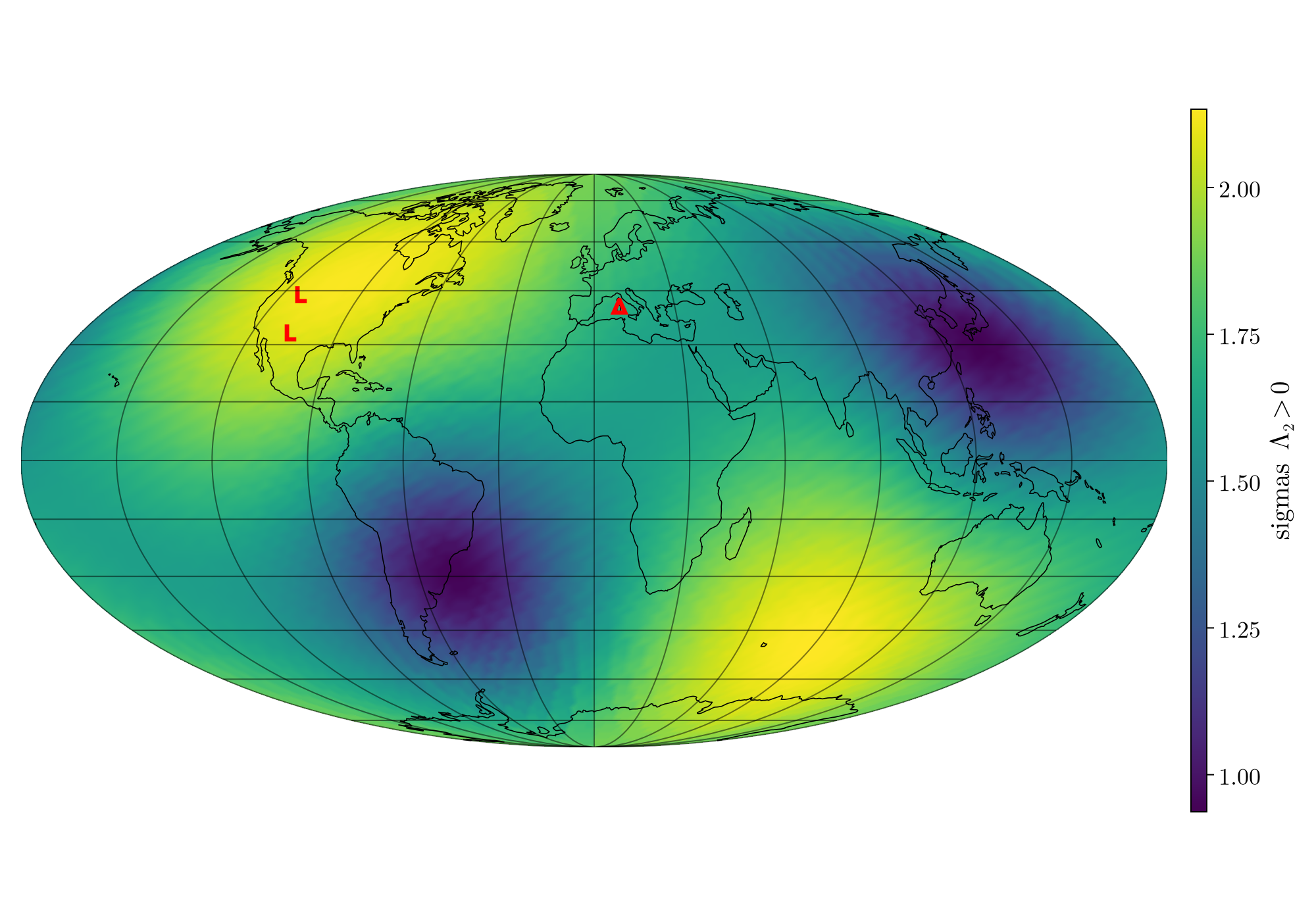
Moreover, we examine the effect of the sky-position for ruling out the PBH hypothesis with tidal effects. We show it in fig.˜8 and we reproduce the procedure used for fig.˜5. The statistical significance of detecting hovers between and , depending on the sky position. The angular modulation resembles that seen in sub-solar mass detection, but with lower overall significance.
Figs. 7–8 show that sky location produces large modulations in the measured significance of both mass-based identification and tidal discrimination. For sub-solar identification (fig. 7), the significance can range from to for the same intrinsic binary at fixed redshift, depending solely on sky position. Tidal effects (fig. 8), being weaker and more localized to the late inspiral, show smaller variation but remain sensitive to directional differences. These modulations imply that the probability of achieving strong discrimination for a given binary depends not only on its masses and redshift, but also on its location relative to the network’s antenna response.
Finally, fig.˜9 summarizes PBH detection prospects in terms of expected event rates and redshift reach. We solely consider mergers of stellar black holes (whose mass is on the axis) with PBH ( axis) in the mass range between 0.1 and 3 solar masses. For the former, we adopt the stellar black hole mass function as modeled by Sicilia et al. [84], which computes an ab initio relic distribution using the SEVN stellar/binary evolution code alongside galaxy formation prescriptions; for the PBH abundance, we instead assume, for a given PBH mass, the maximal-possible abundance of PBHs, i.e., we maximize , assuming a monochromatic mass function, and using the constraints of Ref. [73, 83]. The merger rate functional form we employ follows an analytic estimate of the fitting expression provided in Ref. [85], suitable for phenomenological studies. The dips visible between PBH masses of 0.3 and 1 solar masses are due to the shape of the constraints on the PBH abundance in that mass range.


The left panel shows contours of 1 event per year within a sphere of 1 Gpc radius on the plane of stellar-mass PBH vs light PBH. The right panel, instead, shows the distance, expressed as a redshift, within which one event per year is expected: in other words, for a given choice of the PBH and astrophysical black hole mass, the contours indicate the redshift within which one event per year or more is expected. These figures define the observational frontier for probing the nature of light exotic compact objects using third-generation gravitational-wave observatories.
Note that since 1 Gpc approximately corresponds to , fig.˜9 indicates that in a large swath of parameter space there may be as many as events involving a sub-solar mass object where the mass can be confidently said to be sub-solar and will be detectable with 3G detectors. The left panel shows that mergers in the most favorable mass range (e.g., –) occur at rates of per year within a gigaparsec.
6 Discussion and Conclusions
In this work, we have investigated the prospects for identifying sub-solar mass primordial black holes and distinguishing them from possible astrophysical and exotic compact object impostors using third-generation gravitational-wave detectors such as the Einstein Telescope and Cosmic Explorer. Employing the Fisher matrix formalism, we quantified the maximum redshifts at which sub-solar mass companions can be measured with high significance, as well as the redshift ranges where tidal deformability measurements could exclude the primordial black hole hypothesis.
Our analysis shows that sub-solar mass primordial black holes, if present in binary systems with neutron stars or stellar-mass black holes, will be detectable out to cosmological distances. In particular, we find that black hole–primordial black hole binaries can be observed up to redshift , and in some configurations even farther, while neutron star–primordial black hole binaries are typically detectable out to redshift . These results establish that third-generation detectors will have the sensitivity required to probe sub-solar primordial black holes well beyond the capabilities of the current LIGO–Virgo–KAGRA network.
A central challenge, however, lies in establishing the nature of the detected low-mass compact objects. While primordial black holes are characterized by vanishing tidal deformability (), neutron stars, strange quark stars, and boson stars exhibit finite tidal signatures that depend on their respective equations of state. We have shown that tidal measurements, though in principle decisive, are restricted to the local Universe: even with third-generation sensitivity, confident exclusion of the primordial black hole hypothesis through detection of non-zero tidal effects is possible only for redshifts –, depending on the equation of state and binary configuration. This implies that while mass-based identification of sub-solar objects as primordial black holes can be achieved at high redshift, tidal-based discrimination between primordial black holes and material impostors is fundamentally limited to nearby events.
Our results highlight a dual observational frontier. On the one hand, cosmological reach for sub-solar mass detections offers unprecedented opportunities to map the primordial black hole parameter space, probe early-Universe physics, and test the hypothesis that primordial black holes constitute a fraction of the dark matter. On the other hand, the limited redshift horizon for tidal discrimination underscores the importance of low-redshift, high signal-to-noise events for definitively ruling out non-primordial interpretations. This complementarity suggests that robust population-level inference strategies–combining mass spectra, spin distributions, event rates, and tidal signatures–will be essential for establishing the primordial origin of light black holes.
The analysis presented here relies on several simplifying assumptions, including the use of phenomenological prescriptions for strange quark star and boson star equations of state, waveform models calibrated within limited mass-ratio regimes, and the Fisher matrix approximation. Future work should refine these aspects, for instance by employing Bayesian parameter estimation with full inspiral–merger–ringdown waveforms tailored to exotic compact objects, by incorporating more realistic population models of primordial black holes and exotic compact objects, and by exploring synergies with electromagnetic and cosmological probes.
In conclusion, we find that third-generation gravitational-wave observatories will provide a decisive test on the existence of sub-solar primordial black holes. The detection of a sub-solar mass black hole would be a striking signal of new physics, strongly indicative of a primordial origin. Conversely, detection of finite tidal effects in the same mass range would point toward the realization of exotic states of matter, such as strange quark matter or bosonic condensates. Either outcome would have profound implications for nuclear physics, particle physics, and cosmology, reinforcing the role of gravitational waves as a unique tool for exploring the deep connections between astrophysics and fundamental physics.
Appendix A Technical details
A.1 Fisher formalism
The output of an interferometer is a datastream , which can be expressed as
| (A.1) |
where represents the GW signal and represents the noise, which is characterized by the detector PSD . In fact, after going into Fourier space, one can write
| (A.2) |
where represents the noise in the frequency domain and the symbol is the complex conjugate. We also introduce the scalar-product [63]
| (A.3) |
which is a noise-weighted scalar product between the minimum frequency the maximum frequency which depend on the detector PSD and the maximum frequency of the signal. Before introducing the FIM, we introduce the Signal-to-Noise, which gives a measure of the strength of the signal and, for a single detector, is defined as
| (A.4) |
while for a network of detectors, the SNR is
| (A.5) |
where indicates the different detectors. In this work, we consider a signal to be detected when the network SNR is above a threshold, which we take to be = 8.
Under the assumption that the noise is stationary, Gaussian distributed and with zero mean, the FIM defined as in Eq. (2.1), which in this notation becomes
| (A.6) |
where represents one of the CBC parameters and is the standard Gaussian likelihood (see e.g. [79]) of the datastream measured at the detector given the event parameters . Moreover, indicates the ensemble average over the noise realizations.
A.2 Detectors
The positions and orientations of the detectors are reported in table˜3 while their power spectral densities are plotted in the left panel of fig.˜10.
| Latitude | Longitude | Orientation | |
|---|---|---|---|
| CE 40 km | 43.83 | -112.82 | -45.0 |
| CE 20 km | 33.16 | -106.48 | -105.0 |
| ET 10 km triangular | 40.52 | 9.42 | 0.0 |
A.3 Tidal deformabilities
The mass of the bosonic constituent sets the fundamental mass and length scales of a boson star, with the maximum mass scaling as and the typical radius [54, 80]. The effective EOS arises from the scalar potential: for free bosons the pressure–density relation is entirely determined by the field configuration, while with quartic self-interactions, , one can approximate a polytropic form [25]. Given an assumed EOS, the mass–radius relation is fixed, and thus the compactness , which controls the dimensionless tidal deformability , with the Love number [50]. Lighter bosons generically lead to extended, low-compactness configurations with large , while heavier bosons or strongly self-interacting fields yield more compact stars with suppressed tidal signatures, potentially compatible with gravitational-wave constraints from events such as GW170817 [2]. In our study, we do not impose any theoretical priors on and and the resulting microphysics, but rather assume a phenomenological EOS. In fig.˜10, we show the three EOS used in this work. The SQM3 tidal deformability [91] is similar to the AP3 one, with the significant difference that SQM3 has a maximum mass , while for AP3 . As said in the main text, the BS5 curve reproduces five times the deformability of a AP3 tidal deformability.


Right: Relations of mass of the compact object and their tidal deformability for a strange quark star SQM3 (blue), for a neutron star with EOS AP3 (orange) and for the phenomenological boson star model employed in this work BS5 (green).
Acknowledgments
This work is partly supported by the U.S. Department of Energy grant number de-sc0010107 (SP). AB is supported by ICSC – Centro Nazionale di Ricerca in High Performance Computing, Big Data and Quantum Computing, funded by European Union – NextGenerationEU”. AB would like to thank Stefano Anselmi, Mauro Pieroni, Alessandro Renzi and Angelo Ricciardone for early discussions on the project. AB would like to thank Juan Garcia-Bellido and Sachsa Husa for useful discussions. The authors would also like to thank Liam Colombo Murphy for the strange quark stars EOS solver. The authors would like to thank the anonymous referee for helpful suggestions.
References
- [1] (2025-03) The Science of the Einstein Telescope. External Links: 2503.12263 Cited by: §1, §1, §2.
- [2] (2018) GW170817: Measurements of neutron star radii and equation of state. Phys. Rev. Lett. 121 (16), pp. 161101. External Links: 1805.11581, Document Cited by: §A.3.
- [3] (2018) GW170817: Measurements of neutron star radii and equation of state. Phys. Rev. Lett. 121 (16), pp. 161101. External Links: 1805.11581, Document Cited by: §4.
- [4] (2021-12) Tests of General Relativity with GWTC-3. External Links: 2112.06861 Cited by: §1.
- [5] (2023) GWTC-3: Compact Binary Coalescences Observed by LIGO and Virgo during the Second Part of the Third Observing Run. Phys. Rev. X 13 (4), pp. 041039. External Links: 2111.03606, Document Cited by: §2.
- [6] (2023) Search for subsolar-mass black hole binaries in the second part of Advanced LIGO’s and Advanced Virgo’s third observing run. Mon. Not. Roy. Astron. Soc. 524 (4), pp. 5984–5992. Note: [Erratum: Mon.Not.Roy.Astron.Soc. 526, 6234 (2023)] External Links: 2212.01477, Document Cited by: §1.
- [7] (2020) Planck 2018 results. VI. Cosmological parameters. Astron. Astrophys. 641, pp. A6. Note: [Erratum: Astron.Astrophys. 652, C4 (2021)] External Links: 1807.06209, Document Cited by: §2.
- [8] (1998) The Equation of state of nucleon matter and neutron star structure. Phys. Rev. C 58, pp. 1804–1828. External Links: nucl-th/9804027, Document Cited by: §4.
- [9] (2025-06) Detectability and Parameter Estimation for Einstein Telescope Configurations with GWJulia. External Links: 2506.21530 Cited by: §1, §2, §4.
- [10] (2025-11) Tests of General Relativity with Einstein Telescope. External Links: 2511.07520 Cited by: §2.
- [11] (1998) The properties of strange stars in the quark mass-density-dependent model. Int. J. Mod. Phys. D 7, pp. 29–48. External Links: Document Cited by: 1st item.
- [12] (2016) Fast spinning strange stars: possible ways to constrain interacting quark matter parameters. Mon. Not. Roy. Astron. Soc. 457 (3), pp. 3101–3114. External Links: 1601.06120, Document Cited by: §3.1.
- [13] (2009) Relativistic theory of tidal Love numbers. Phys. Rev. D 80, pp. 084018. External Links: 0906.1366, Document Cited by: §1, §1, 2nd item.
- [14] (1971) Collapsed nuclei. Phys. Rev. D 4, pp. 1601–1606. External Links: Document Cited by: §3.1.
- [15] (2024) Listening to the Universe with next generation ground-based gravitational-wave detectors. Phys. Rev. D 110 (8), pp. 083040. External Links: 2202.11048, Document Cited by: §1.
- [16] (2021) GWBENCH: a novel Fisher information package for gravitational-wave benchmarking. Class. Quant. Grav. 38 (17), pp. 175014. External Links: 2010.15202, Document Cited by: §1.
- [17] (2009) Comparison of high-accuracy numerical simulations of black-hole binaries with stationary phase post-Newtonian template waveforms for Initial and Advanced LIGO. Class. Quant. Grav. 26, pp. 114006. External Links: 0901.1628, Document Cited by: §4.
- [18] (2009) Comparison of post-Newtonian templates for compact binary inspiral signals in gravitational-wave detectors. Phys. Rev. D 80, pp. 084043. External Links: 0907.0700, Document Cited by: §4.
- [19] (1974) Black holes in the early Universe. Mon. Not. Roy. Astron. Soc. 168, pp. 399–415. Cited by: §1, §3.4.
- [20] (2024) Primordial Black Holes as a Probe of Cosmology and High Energy Physics. Phys. Rept. 1054, pp. 1–67. External Links: 2306.03903, Document Cited by: §3.4.
- [21] (2016) Primordial Black Holes as Dark Matter. Phys. Rev. D 94, pp. 083504. External Links: 1607.06077, Document Cited by: §3.4.
- [22] (2020) Neutron star tidal deformability and equation of state constraints. Gen. Rel. Grav. 52 (11), pp. 109. External Links: 2006.03168, Document Cited by: §1.
- [23] (2011) Mass-radius relation of Newtonian self-gravitating Bose-Einstein condensates with short-range interactions: I. Analytical results. Phys. Rev. D 84, pp. 043531. External Links: 1103.2050, Document Cited by: 2nd item.
- [24] (2017) Spin Distribution of Primordial Black Holes. PTEP 2017 (8), pp. 083E01. External Links: 1704.06573, Document Cited by: §3.4.
- [25] (1986) Boson Stars: Gravitational Equilibria of Selfinteracting Scalar Fields. Phys. Rev. Lett. 57, pp. 2485–2488. External Links: Document Cited by: §A.3, §1, 1st item.
- [26] (2024) Can we identify primordial black holes? Tidal tests for subsolar-mass gravitational-wave observations. Phys. Rev. D 109 (12), pp. 124063. External Links: 2402.18656, Document Cited by: §1, §1, §1.
- [27] (2025) Cosmology and nuclear physics implications of a subsolar gravitational-wave event. Phys. Rev. D 111 (8), pp. 083538. External Links: 2408.14287, Document Cited by: §1, §1, §1.
- [28] (2020) Relativistic Shapiro delay measurements of an extremely massive millisecond pulsar. Nature Astronomy 4, pp. 72–76. External Links: Document, 1904.06759 Cited by: 1st item.
- [29] (1994) Gravitational waves from merging compact binaries: How accurately can one extract the binary’s parameters from the inspiral wave form?. Phys. Rev. D 49, pp. 2658–2697. External Links: gr-qc/9402014, Document Cited by: §1, §2.
- [30] (2012) Measurability of the tidal polarizability of neutron stars in late-inspiral gravitational-wave signals. Phys. Rev. D 85, pp. 123007. External Links: 1203.4352, Document Cited by: §1.
- [31] (2009) Relativistic tidal properties of neutron stars. Phys. Rev. D 80, pp. 084035. External Links: 0906.0096, Document Cited by: 2nd item.
- [32] (2020) The Evolution of Primordial Black Holes and their Spins. JCAP 04, pp. 052. External Links: 1909.03883, Document Cited by: §3.4.
- [33] (2024) Flea on the elephant: Tidal Love numbers in subsolar primordial black hole searches. Phys. Rev. D 110 (10), pp. 104041. External Links: 2408.14207, Document Cited by: §1, §1.
- [34] (2023) GWDALI: A Fisher-matrix based software for gravitational wave parameter-estimation beyond Gaussian approximation. Astron. Comput. 45, pp. 100759. External Links: 2307.10154, Document Cited by: §1.
- [35] (2019) Improving the NRTidal model for binary neutron star systems. Phys. Rev. D 100 (4), pp. 044003. External Links: 1905.06011, Document Cited by: §4.
- [36] (2023) gwfish: A simulation software to evaluate parameter-estimation capabilities of gravitational-wave detector networks. Astron. Comput. 42, pp. 100671. External Links: 2205.02499, Document Cited by: §1.
- [37] (2025) Validating prior-informed Fisher-matrix analyses against GWTC data. Phys. Rev. D 111 (2), pp. 024036. External Links: 2404.16103, Document Cited by: §2.
- [38] (2021) A Horizon Study for Cosmic Explorer: Science, Observatories, and Community. External Links: 2109.09882 Cited by: §1.
- [39] (2024-09) Gravitational-Wave Data Analysis with High-Precision Numerical Relativity Simulations of Boson Star mergers. Physical Review Letters 133 (13), pp. 131401. Note: arXiv:2406.02715 [gr-qc]Comment: 7+8 pages (incl.supplementary material), 7 figures, 3 tables, to match version published in Physical Review Letters External Links: ISSN 0031-9007, 1079-7114, Link, Document Cited by: §5.
- [40] (1992) Detection, measurement and gravitational radiation. Phys. Rev. D 46, pp. 5236–5249. External Links: gr-qc/9209010, Document Cited by: §1, §2.
- [41] (2022) How to assess the primordial origin of single gravitational-wave events with mass, spin, eccentricity, and deformability measurements. Phys. Rev. D 105 (6), pp. 063510. External Links: 2112.10660, Document Cited by: §3.4.
- [42] (2024) Fully precessing higher-mode surrogate model of effective-one-body waveforms. Phys. Rev. D 110 (12), pp. 124038. External Links: 2203.00381, Document Cited by: §5.
- [43] (2021) Waveform systematics in the gravitational‐wave inference of tidal parameters and equation of state from binary neutron star signals. Phys. Rev. D 103 (12), pp. 124015. External Links: Document, arXiv:2009.08467 Cited by: §1.
- [44] (2020) Multimode frequency-domain model for the gravitational wave signal from nonprecessing black-hole binaries. Phys. Rev. D 102 (6), pp. 064002. External Links: 2001.10914, Document Cited by: footnote 1.
- [45] (2016) Hunting for Dark Particles with Gravitational Waves. JCAP 10, pp. 001. External Links: 1605.01209, Document Cited by: §1.
- [46] (2021) Primordial Black Holes as a dark matter candidate. J. Phys. G 48 (4), pp. 043001. External Links: 2007.10722, Document Cited by: §3.4.
- [47] (2015) No-hair theorem for Black Holes in Astrophysical Environments. Phys. Rev. Lett. 114 (15), pp. 151102. External Links: 1503.03240, Document Cited by: §1.
- [48] (2017) Spins of primordial black holes formed in the matter-dominated phase of the Universe. Phys. Rev. D 96, pp. 083517. External Links: 1707.03595, Document Cited by: §3.4.
- [49] (1971) Gravitationally collapsed objects of very low mass. Mon. Not. Roy. Astron. Soc. 152, pp. 75. Cited by: §1, §3.4.
- [50] (2008) Tidal Love numbers of neutron stars. Astrophys. J. 677, pp. 1216–1220. External Links: 0711.2420, Document Cited by: §A.3.
- [51] (2016) Frequency-domain gravitational waves from nonprecessing black-hole binaries. I. New numerical waveforms and anatomy of the signal. Phys. Rev. D 93 (4), pp. 044006. External Links: 1508.07250, Document Cited by: §4.
- [52] (2022) Forecasting the Detection Capabilities of Third-generation Gravitational-wave Detectors Using GWFAST. Astrophys. J. 941 (2), pp. 208. External Links: 2207.02771, Document Cited by: §1.
- [53] (2025) A Search for Low-mass Neutron Stars in the Third Observing Run of Advanced LIGO and Virgo. Astrophys. J. 984 (1), pp. 61. External Links: 2412.05369, Document Cited by: 1st item.
- [54] (1968) Klein-Gordon Geon. Phys. Rev. 172, pp. 1331–1342. External Links: Document Cited by: §A.3, 1st item.
- [55] (2016) Frequency-domain gravitational waves from nonprecessing black-hole binaries. II. A phenomenological model for the advanced detector era. Phys. Rev. D 93 (4), pp. 044007. External Links: 1508.07253, Document Cited by: §4.
- [56] (2012) Stable Phases of Boson Stars. Phys. Rev. D 85, pp. 024045. External Links: 1109.5858, Document Cited by: 2nd item.
- [57] (2024) Recalibrating a gravitational wave phenomenological waveform model. Phys. Rev. D 109 (12), pp. 124009. External Links: 2306.17245, Document Cited by: §5.
- [58] (2001) Neutron star structure and the equation of state. Astrophys. J. 550, pp. 426. External Links: astro-ph/0002232, Document Cited by: §3.3.
- [59] (2004) The physics of neutron stars. Science 304, pp. 536–542. External Links: astro-ph/0405262, Document Cited by: §3.3.
- [60] (2022) Exploring the sky localization and early warning capabilities of third generation gravitational wave detectors in three-detector network configurations. Phys. Rev. D 105 (4), pp. 043010. External Links: 2109.07389, Document Cited by: §1.
- [61] (2018) LVK Algorithm Library - LALSuite. Note: Free software (GPL) External Links: Document Cited by: §4, §4.
- [62] (2020) Science Case for the Einstein Telescope. JCAP 03, pp. 050. External Links: 1912.02622, Document Cited by: §1.
- [63] (2008) Gravitational waves. Vol. 2, Oxford university press. Cited by: §A.1.
- [64] (2021) Bayesian Inference of Strange Star Equation of State Using the GW170817 and GW190425 Data. Astrophys. J. Lett. 917 (2), pp. L22. External Links: 2107.13997, Document Cited by: 2nd item.
- [65] (2022) Broad search for gravitational waves from subsolar-mass binaries through LIGO and Virgo’s third observing run. Phys. Rev. D 106 (2), pp. 023024. External Links: 2202.11024, Document Cited by: §1.
- [66] (2011) Reliability of complete gravitational waveform models for compact binary coalescences. Phys. Rev. D 84, pp. 064029. External Links: 1107.0996, Document Cited by: §5.
- [67] (2022) Ranking Love Numbers for the Neutron Star Equation of State: The Need for Third-Generation Detectors. Phys. Rev. Lett. 128 (10), pp. 101101. External Links: 2104.10035, Document Cited by: §1, §4.
- [68] (2008) A Data-analysis driven comparison of analytic and numerical coalescing binary waveforms: Nonspinning case. Phys. Rev. D 77, pp. 024014. External Links: 0704.1964, Document Cited by: §4.
- [69] (2015) Aligned spin neutron star-black hole mergers: a gravitational waveform amplitude model. Phys. Rev. D 92 (8), pp. 084050. External Links: 1509.00512, Document Cited by: §4.
- [70] (2023) Role of Quark Matter and Color Superconductivity in the Structure and Tidal Deformability of Strange Dwarfs. Universe 9 (9), pp. 382. External Links: Document Cited by: §1.
- [71] (2015) Tidal deformation of a slowly rotating black hole. Phys. Rev. D 91, pp. 044004. External Links: 1404.2192, Document Cited by: 2nd item.
- [72] (2010) Tidal love numbers of neutron and self-bound quark stars. Phys. Rev. D 82, pp. 024016. External Links: Document Cited by: §1, §1, §1, §1.
- [73] (2017) CMB bounds on dark matter including s as a candidate. Phys. Rev. D 96, pp. 083524. External Links: Document, 1707.04206 Cited by: §5.
- [74] (1995) Quark - hadron phase transition in protoneutron stars. Phys. Rev. D 52, pp. 661–665. External Links: Document Cited by: §3.1, §4, §5.
- [75] (2020) Setting the cornerstone for a family of models for gravitational waves from compact binaries: The dominant harmonic for nonprecessing quasicircular black holes. Phys. Rev. D 102 (6), pp. 064001. External Links: 2001.11412, Document Cited by: Table 2, §4, §5.
- [76] (2010) The Einstein Telescope: A third-generation gravitational wave observatory. Class. Quant. Grav. 27, pp. 194002. External Links: Document Cited by: §1.
- [77] (2019) Cosmic Explorer: The U.S. Contribution to Gravitational-Wave Astronomy beyond LIGO. Bull. Am. Astron. Soc. 51 (7), pp. 035. External Links: 1907.04833 Cited by: §1.
- [78] (2024) Gravitational wave surrogate model for spinning, intermediate mass ratio binaries based on perturbation theory and numerical relativity. Phys. Rev. D 110 (12), pp. 124069. External Links: 2407.18319, Document Cited by: §5.
- [79] (2013) Inadequacies of the Fisher Information Matrix in gravitational-wave parameter estimation. Phys. Rev. D 88 (8), pp. 084013. External Links: 1308.1397, Document Cited by: §A.1, §1.
- [80] (1969) Systems of selfgravitating particles in general relativity and the concept of an equation of state. Phys. Rev. 187, pp. 1767–1783. External Links: Document Cited by: §A.3.
- [81] (2003) General relativistic boson stars. Class. Quant. Grav. 20, pp. R301–R356. External Links: Document, 0801.0307 Cited by: §3.2.
- [82] (2017) Distinguishing Boson Stars from Black Holes and Neutron Stars from Tidal Interactions in Inspiraling Binary Systems. Phys. Rev. D 96, pp. 024002. External Links: 1704.08651, Document Cited by: §1.
- [83] (2020) Probing pbh dark matter with radio and x-ray observations. Phys. Rev. Res. 2, pp. 023204. External Links: Document, 2002.10771 Cited by: §5.
- [84] (2022) The Black Hole Mass Function Across Cosmic Times. I. Stellar Black Holes and Light Seed Distribution. Astrophys. J. 924 (2), pp. 56. External Links: 2110.15607, Document Cited by: §5.
- [85] (2024) Redshift evolution of primordial black hole merger rate. Phys. Rev. D 109 (12), pp. 123546. External Links: 2403.11325, Document Cited by: §5.
- [86] (2018) On the minimum mass of neutron stars. Mon. Not. Roy. Astron. Soc. 481, pp. 3305. External Links: 1808.02368, Document Cited by: 1st item.
- [87] (2020) Modeling the gravitational wave signature of neutron star black hole coalescences. Phys. Rev. D 101 (12), pp. 124059. External Links: 2002.08383, Document Cited by: §4.
- [88] (2008) Use and abuse of the Fisher information matrix in the assessment of gravitational-wave parameter-estimation prospects. Phys. Rev. D 77, pp. 042001. External Links: gr-qc/0703086, Document Cited by: §1, §2, §2, §2.
- [89] (2011) Post-1-newtonian tidal effects in the gravitational waveform from binary inspirals. Phys. Rev. D 83, pp. 084051. External Links: Document Cited by: §1.
- [90] (2018) Constraints on the Primordial Black Hole Abundance from the First Advanced LIGO Observation Run Using the Stochastic Gravitational-Wave Background. Phys. Rev. Lett. 120 (19), pp. 191102. External Links: 1610.08725, Document Cited by: §1.
- [91] (2021) Tidal deformability of strange quark planets and strange dwarfs. Physical Review D 104 (12), pp. 123028. Cited by: §A.3.
- [92] (1984) Cosmic Separation of Phases. Phys. Rev. D 30, pp. 272–285. External Links: Document Cited by: §1, §3.1.
- [93] (1997) Rotating boson stars in general relativity. Phys. Rev. D 56, pp. 762–771. External Links: Document Cited by: §1, §3.2.
- [94] (2000) On the mass of moderately rotating strange stars. Astron. Astrophys. 359, pp. 311–314. External Links: astro-ph/0004375 Cited by: 1st item.
- [95] (2018) Constraints on interquark interaction parameters with GW170817 in a binary strange star scenario. Phys. Rev. D 97 (8), pp. 083015. External Links: 1711.04312, Document Cited by: 2nd item.