跳到论文正文
W Papers独立论文阅读器 arXiv:2507.18443 论文正文 计算阅读时间 · 0%
引用这篇论文根据当前论文元数据生成,正式投稿前建议核对。


On MAP estimates and source conditions for drift identification in SDEs

Daniel Tenbrinck    Nikolas Uesseler    Philipp Wacker    Benedikt Wirth
Abstract

We consider the inverse problem of identifying the drift in an SDE from nn observations of its solution at M+1M+1 distinct time points. We derive a corresponding MAP estimate, we prove differentiability properties as well as a so-called tangential cone condition for the forward operator, and we review the existing theory for related problems, which under a slightly stronger tangential cone condition would additionally yield convergence rates for the MAP estimate as n→∞n\to\infty. Numerical simulations in 1D indicate that such convergence rates indeed hold true.

1 Introduction

We are consider the following problem. At fixed time points 0=t0<t1<…<tM=T0=t_{0}<t_{1}<\ldots<t_{M}=T we observe the position of nn distinguishable particles which stochastically move around in some bounded smooth domain Ω⊂ℝd\Omega\subset\mathbb{R}^{d}. From this observation we aim to estimate the drift μ:Ω→ℝd\mu:\Omega\to\mathbb{R}^{d} in the stochastic differential equation (SDE)

d​Xt=μ​(Xt)​d​t+σ​d​Wt{\mathrm{d}}X_{t}=\mu(X_{t}){\mathrm{d}}t+\sigma{\mathrm{d}}W_{t} (1)

that governs the motion of each particle (WtW_{t} denotes the Wiener process with reflection at ∂Ω\partial\Omega and σ>0\sigma>0 a known coefficient; furthermore we assume the normal component μ⋅ν\mu\cdot\nu of the drift to vanish on the boundary ∂Ω\partial\Omega). Our aim is to develop and analyse a corresponding Bayesian maximum a posteriori (MAP) estimate.

An example application for which this inverse problem is relevant is the probing of tissue properties in zebrafish embryos: During embryonic development, so-called primordial germ cells (PGCs) migrate from the location of their differentiation to the site where the gonads develop. However, if directional migration is abolished in those cells by genetic modification, they migrate randomly within the embryo [9]. The drift μ\mu then indicates areas of in-/decreased cell attraction within the embryo (cf. fig.˜1).

Refer to caption
Figure 1: Left: Epifluorescence microscopy data of a zebrafish embryo (PGCs in red). Right: PGC distribution after registration of 934 embryos reveals anatomical structures as barrier for cells [9].

As usual, our MAP estimate will be the minimizer of the (slightly modified) log-posterior

μ↦Sτ​(F​(μ),Gn)+α​‖μ‖Hr2,\mu\mapsto S_{\tau}(F(\mu),G^{n})+\alpha\|\mu\|_{H^{r}}^{2},

where GnG^{n} is the empirical measure of the observed particles, the forward operator FF yields the probability density of particle observations under a given drift μ\mu, SS is the cross-entropy and SτS_{\tau} a shifted version, and α>0\alpha>0 a regularization parameter. The parameter identification being a nonlinear inverse problem, we are interested in whether or under what conditions one can obtain rates for how fast the minimizer of the above functional converges to the ground truth μ†\mu^{\dagger} as the particle number nn increases to infinity and the regularization weight α\alpha is decreased correspondingly. To this end we extensively review the existing theory and perform first steps to applying this theory to our setting:

  • •

    We give an overview of the historical development of source and nonlinearity conditions for nonlinear inverse problems, culminating in variational source conditions that are particularly pertinent to our framework (sections˜2 and 3).

  • •

    We next present the forward operator relevant to our study and derive the corresponding log-likelihood for the associated inverse problem (section˜4).

  • •

    The following sections review theoretical results from [4] (which considered the stationary version of our inverse problem) on stochastic convergence rates in the context of stochastic inverse problems, highlighting how these (albeit non-explicit) rates may be established using the variational source conditions previously discussed and tailored to our specific setup (sections˜5 and 6).

  • •

    Within this framework, the variational source conditions can be reduced to a tangential cone condition. In the penultimate section, we prove a weaker form of this condition; although it does not suffice to guarantee convergence rates, it nevertheless provides supporting evidence that such rates may hold (section˜7).

  • •

    We conclude by presenting numerical experiments that illustrate and support our theoretical findings (section˜8).

2 Historical note on convergence rates for nonlinear inverse problems

In their 1988 paper [17], Seidmann and Vogel extended the theory of ill-posed problems to the case of nonlinear operators F:X→YF:X\to Y. As an approximate solution to F​(x)=yδF(x)=y^{\delta} for some noisy measurement yδy^{\delta} they consider the minimizer xαδx_{\alpha}^{\delta} of the Tikhonov functional

Tαyδ​(x):=‖F​(x)−yδ‖2+α​‖x−x⋆‖2for ​x∈X​ and some fixed ​x∗∈XT_{\alpha}^{y^{\delta}}(x)\vcentcolon=\|F(x)-y^{\delta}\|^{2}+\alpha\|x-x^{\star}\|^{2}\quad\text{for }x\in X\text{ and some fixed }x^{*}\in X

and study its existence, stability, and convergence to the ground truth x†=F−1​(y†)x^{\dagger}=F^{-1}(y^{\dagger}) for yδ→y†y^{\delta}\to y^{\dagger} and an appropriate choice of the regularization parameter α>0\alpha>0. In 1989, Engl, Kunisch, and Neubauer then published the first result on corresponding convergence rates [5], for which one needs to impose so-called source conditions on the ground truth. In this section we give a historical account on the development of these ideas to the later employed so-called variational source condition.

The convergence of Tikhonov regularization can be arbitrarily slow without a source condition, the concept of which we briefly motivate: Assume that x†x^{\dagger} is an x⋆x^{\star}-minimum norm solution, i.e. a solution of

minimize12​‖x⋆−x‖2subject toF​(x)=y†.\textit{minimize}\qquad\tfrac{1}{2}\|x^{\star}-x\|^{2}\qquad\text{subject to}\qquad F(x)=y^{\dagger}. (2)

Naturally we can consider the Lagrangian

L​(ω,x)=12​‖x⋆−x‖2+⟨ω,F​(x)−y†⟩for ​x∈X,ω∈Y∗.L(\omega,x)=\tfrac{1}{2}\|x^{\star}-x\|^{2}+\langle\omega,F(x)-y^{\dagger}\rangle\quad\text{for }x\in X,\ \omega\in Y^{*}.

Let us assume that FF is Fréchet-differentiable and that strong duality holds, i.e. if x†∈Xx^{\dagger}\in X minimizes (2) then there exists ω^∈Y∗\hat{\omega}\in Y^{*} such that (ω^,x†)(\hat{\omega},x^{\dagger}) is a saddle point of LL. In particular, under this assumption it holds

∂∂x​L​(ω^,x)|x†=0or equivalentlyx⋆−x†=F′​(x†)#​ω^,\tfrac{\partial}{\partial x}L(\hat{\omega},x)|_{x^{\dagger}}=0\qquad\text{or equivalently}\qquad x^{\star}-x^{\dagger}=F^{\prime}(x^{\dagger})^{\#}\hat{\omega},

understood as an equality in X∗X^{*}. For instance, in the case of x⋆=0x^{\star}=0 and linear compact FF between Hilbert spaces X,YX,Y we arrive at the well-known source condition x†=F#​ω^=(F#​F)12​px^{\dagger}=F^{\#}\hat{\omega}=(F^{\#}F)^{\frac{1}{2}}p for some p∈Xp\in X, which is to be understood as imposed regularity of x†x^{\dagger} measured in terms of FF. Thus, this regularity assumption is generalized by the assumption of strong duality, which, for the general nonlinear problem, indeed allows to achieve convergence rates. Let us summarize the result from [5].

Assumption 2.1 (Conditions for convergence rates I, [5]).
  1. 1.

    Let X,YX,Y be Hilbert spaces and F:X→YF:X\to Y Fréchet-differentiable.

  2. 2.

    Let x†x^{\dagger} be an x⋆x^{\star}-minimum norm solution that fulfils the following source condition: There exists ω∈Y\omega\in Y satisfying

    x†−x⋆=F′​(x†)#​ω.x^{\dagger}-x^{\star}=F^{\prime}(x^{\dagger})^{\#}\omega.
  3. 3.

    Let F′F^{\prime} fulfil the following Lipschitz condition: There exists L<1/‖ω‖L<1/\|\omega\| with

    ‖F′​(x†)−F′​(z)‖≤L​‖x†−z‖ for all ​z∈X.\|F^{\prime}(x^{\dagger})-F^{\prime}(z)\|\leq L\|x^{\dagger}-z\|\qquad\text{ for all }z\in X.
Theorem 2.2 (Convergence rate I, [5, Thm. 2.4]).

Let assumption 2.1 hold and ‖yδ−y†‖≤δ\|y^{\delta}-y^{\dagger}\|\leq\delta. Then for the choice α∼δ\alpha\sim\delta it holds ‖xαδ−x†‖≲δ.\|x_{\alpha}^{\delta}-x^{\dagger}\|\lesssim\sqrt{\delta}.

The next step, made by Burger and Osher in 2004 [3], was to replace the squared Hilbert space norm ‖x−x⋆‖2\|x-x^{\star}\|^{2} by a general convex penalty functional JJ, in which case one can still estimate the reconstruction error in terms of the Bregman distance

𝒟Jξ​(x,x†)=J​(x)−J​(x†)−⟨ξ,x−x†⟩≥0for ​ξ∈∂J​(x†).\mathcal{D}_{J}^{\xi}(x,x^{\dagger})=J(x)-J(x^{\dagger})-\langle\xi,x-x^{\dagger}\rangle\geq 0\qquad\text{for }\xi\in\partial J(x^{\dagger}).

As before, let x†x^{\dagger} be a JJ-minimizing solution of F​(x)=y†F(x)=y^{\dagger} and consider the corresponding Lagrangian

L​(ω,x)=J​(x)+⟨ω,F​(x)−y†⟩.\displaystyle L(\omega,x)=J(x)+\langle\omega,F(x)-y^{\dagger}\rangle.

Now the strong duality assumption is equivalent to the existence of a Lagrange multiplier ω\omega such that (ω,x†)(\omega,x^{\dagger}) is a saddle point of the Lagrangian, which with convexity of JJ and differentiability of FF implies the (generalized) source condition

F′​(x†)#​ω∈∂J​(x†).\displaystyle F^{\prime}(x^{\dagger})^{\#}\omega\in\partial J(x^{\dagger}).

Again, a condition controlling the nonlinearity of operator FF is needed in addition.

Assumption 2.3 (Conditions for convergence rates II, [3]).
  1. 1.

    Let XX be a Banach space carrying also a potentially weaker topology τX\tau_{X}, YY a Hilbert space, and F:X→YF:X\to Y sequentially continuous w.r.t. τX\tau_{X} and Fréchet-differentiable. Let JJ be convex and sequentially lower semi-continuous w.r.t. τX\tau_{X} with τX\tau_{X}-sequentially precompact sublevel sets.

  2. 2.

    Let x†x^{\dagger} be a JJ-minimizing solution that fulfils the following source condition: There exists ω∈Y\omega\in Y satisfying

    ξ:=F′​(x†)#​ω∈∂J​(x†).\displaystyle\xi\vcentcolon=F^{\prime}(x^{\dagger})^{\#}\omega\in\partial J(x^{\dagger}).
  3. 3.

    Let FF fulfil the following nonlinearity condition: There exists η>0\eta>0

    ⟨F​(z)−F​(x†)−F′​(x†)​(z−x†),ω⟩≤η​‖F​(x†)−F​(z)‖​‖ω‖\displaystyle\langle F(z)-F(x^{\dagger})-F^{\prime}(x^{\dagger})(z-x^{\dagger}),\omega\rangle\leq\eta\|F(x^{\dagger})-F(z)\|\|\omega\| for all ​z∈X.\displaystyle\text{ for all }z\in X.
Theorem 2.4 (Convergence rate II, [3, Sec. 3.3]).

Let assumption 2.3 hold and ‖yδ−y†‖≤δ\|y^{\delta}-y^{\dagger}\|\leq\delta. Then for the choice α∼δ\alpha\sim\delta it holds 𝒟Jξ​(xαδ,x†)≲δ\mathcal{D}_{J}^{\xi}(x_{\alpha}^{\delta},x^{\dagger})\lesssim\delta.

In 2006, Resmerita and Scherzer [16] allowed also YY to be Banach and replaced the nonlinearity control on FF by a Bregman distance.

Assumption 2.5 (Conditions for convergence rates III, [16]).
  1. 1.

    Let X,YX,Y be Banach spaces, both carrying potentially weaker topologies τX\tau_{X} and τY\tau_{Y}, and F:X→YF:X\to Y sequentially continuous w.r.t. τX\tau_{X} and τY\tau_{Y} and Fréchet-differentiable. Let JJ be convex and sequentially lower semi-continuous w.r.t. τX\tau_{X} with τX\tau_{X}-sequentially precompact sublevel sets, and let the norm on YY be sequentially lower semi-continuous w.r.t. τY\tau_{Y}.

  2. 2.

    Let x†x^{\dagger} be a JJ-minimizing solution that fulfils the following source condition: There exists ω∈Y\omega\in Y satisfying

    ξ:=F′​(x†)#​ω∈∂J​(x†).\displaystyle\xi\vcentcolon=F^{\prime}(x^{\dagger})^{\#}\omega\in\partial J(x^{\dagger}).
  3. 3.

    Let FF fulfil the following nonlinearity condition: There exists η<1/‖ω‖\eta<1/\|\omega\|

    ‖F​(x)−F​(x†)−F′​(x†)​(x−x†)‖≤η​𝒟Jξ​(x,x†) for all ​x∈X.\|F(x)-F(x^{\dagger})-F^{\prime}(x^{\dagger})(x-x^{\dagger})\|\leq\eta\mathcal{D}_{J}^{\xi}(x,x^{\dagger})\qquad\text{ for all }x\in X.
Theorem 2.6 (Convergence rate III, [16, Thm. 3.2]).

Let assumption 2.5 hold and ‖yδ−y†‖≤δ\|y^{\delta}-y^{\dagger}\|\leq\delta. Then for the choice α∼δ\alpha\sim\delta it holds ‖F​(xαδ)−F​(x†)‖≲δ\|F(x_{\alpha}^{\delta})-F(x^{\dagger})\|\lesssim\delta and 𝒟Jξ​(xαδ,x†)≲δ.\mathcal{D}_{J}^{\xi}(x_{\alpha}^{\delta},x^{\dagger})\lesssim\delta.

To this point the nonlinearity conditions on FF and the source conditions on x†x^{\dagger} require differentiability of FF at x†x^{\dagger}. In 2007, Hofmann, Kaltenbacher, Pöschl, and Scherzer managed to remove this restriction via a reformulation as a variational inequality [10], arriving at a so-called variational source condition. They also slightly generalize the Tikhonov functional to

Tαδ​(x):=‖F​(x)−yδ‖p+α​J​(x) for ​p>1.T_{\alpha}^{\delta}(x)\vcentcolon=\|F(x)-y^{\delta}\|^{p}+\alpha J(x)\qquad\text{ for }p>1. (3)
Assumption 2.7 (Conditions for convergence rates IV, [10]).
  1. 1.

    Let assumption 2.5 (1) hold, except Fréchet differentiability of FF is no longer required.

  2. 2.

    Let x†x^{\dagger} be a JJ-minimizing solution, and let there exist ξ∈∂J​(x†)\xi\in\partial J(x^{\dagger}), β1∈[0,1)\beta_{1}\in[0,1) and β2≥0\beta_{2}\geq 0 such that

    −⟨ξ,x−x†⟩≤β1​𝒟Jξ​(x,x†)+β2​‖F​(x)−F​(x†)‖ for all ​x∈X.-\langle\xi,x-x^{\dagger}\rangle\leq\beta_{1}\mathcal{D}_{J}^{\xi}(x,x^{\dagger})+\beta_{2}\|F(x)-F(x^{\dagger})\|\qquad\text{ for all }x\in X.
Remark 2.8 (Source and nonlinearity condition imply variational source condition).

Each of the previous assumptions implies assumption 2.7, so the latter is the weakest. Indeed, assumption 2.5 is already weaker than assumption 2.1, and given assumption 2.5 or 2.3 we can argue as follows: Pick ξ=F′​(x†)#​ω\xi=F^{\prime}(x^{\dagger})^{\#}\omega, then

⟨ξ,x−x†⟩=⟨ω,F′​(x†)​(x−x†)+F​(x†)−F​(x)⟩+⟨ω,F​(x)−F​(x†)⟩,\langle\xi,x-x^{\dagger}\rangle=\langle\omega,F^{\prime}(x^{\dagger})(x-x^{\dagger})+F(x^{\dagger})-F(x)\rangle+\langle\omega,F(x)-F(x^{\dagger})\rangle,

which under assumption 2.3 results in

−⟨ξ,x−x†⟩≤η​‖ω‖​‖F​(x†)−F​(x)‖+‖ω‖​‖F​(x)−F​(x†)‖=(1+η)​‖ω‖⏟=⁣:β2​‖F​(x†)−F​(x)‖-\langle\xi,x-x^{\dagger}\rangle\leq\eta\|\omega\|\|F(x^{\dagger})-F(x)\|+\|\omega\|\|F(x)-F(x^{\dagger})\|=\underbrace{(1+\eta)\|\omega\|}_{=\vcentcolon\beta_{2}}\|F(x^{\dagger})-F(x)\|

and under assumption 2.5 results in

−⟨ξ,x−x†⟩≤‖ω‖​‖F′​(x†)​(x−x†)+F​(x†)−F​(x)‖+‖ω‖​‖F​(x)−F​(x†)‖≤η​‖ω‖⏟=⁣:β1​𝒟Jξ​(x,x†)+‖ω‖⏟=⁣:β2​‖F​(x)−F​(x†)‖.-\langle\xi,x-x^{\dagger}\rangle\leq\|\omega\|\|F^{\prime}(x^{\dagger})(x-x^{\dagger})+F(x^{\dagger})-F(x)\|+\|\omega\|\|F(x)-F(x^{\dagger})\|\leq\underbrace{\eta\|\omega\|}_{=\vcentcolon\beta_{1}}\mathcal{D}_{J}^{\xi}(x,x^{\dagger})+\underbrace{\|\omega\|}_{=\vcentcolon\beta_{2}}\|F(x)-F(x^{\dagger})\|.
Theorem 2.9 (Convergence rate IV, [10, Thm. 4.4]).

Let assumption 2.7 hold and ‖yδ−y†‖≤δ\|y^{\delta}-y^{\dagger}\|\leq\delta. Then for the choice α∼δp−1\alpha\sim\delta^{p-1} it holds ‖F​(xαδ)−F​(x†)‖≲δ\|F(x_{\alpha}^{\delta})-F(x^{\dagger})\|\lesssim\delta and 𝒟Jξ​(xαδ,x†)≲δ.\mathcal{D}_{J}^{\xi}(x_{\alpha}^{\delta},x^{\dagger})\lesssim\delta.

In his 2009 joint work with Yamamoto [11], Hofmann himself points out a slight generalization of theorem 2.9 in which the only change is a relaxation of the nonlinearity condition by some exponent κ\kappa.

Assumption 2.10 (Conditions for convergence rates V, [11]).
  1. 1.

    Let assumption 2.7 (1) hold.

  2. 2.

    Let x†x^{\dagger} be a JJ-minimizing solution, and let there exist ξ∈∂J​(x†)\xi\in\partial J(x^{\dagger}), β1∈[0,1)\beta_{1}\in[0,1), β2≥0\beta_{2}\geq 0, and κ∈(0,1]\kappa\in(0,1] such that

    −⟨ξ,x−x†⟩≤β1​𝒟Jξ​(x,x†)+β2​‖F​(x)−F​(x†)‖κ for all ​x∈X.-\langle\xi,x-x^{\dagger}\rangle\leq\beta_{1}\mathcal{D}_{J}^{\xi}(x,x^{\dagger})+\beta_{2}\|F(x)-F(x^{\dagger})\|^{\kappa}\qquad\text{ for all }x\in X.
Theorem 2.11 (Convergence rate V, [11, Thm. 3.3]).

Let assumption 2.10 hold and ‖yδ−y†‖≤δ\|y^{\delta}-y^{\dagger}\|\leq\delta. Then for the choice α∼δp−κ\alpha\sim\delta^{p-\kappa} it holds 𝒟Jξ​(xαδ,x†)∼δκ.\mathcal{D}_{J}^{\xi}(x_{\alpha}^{\delta},x^{\dagger})\sim\delta^{\kappa}.

This result suggests that the variational inequality as well as the Tikhonov functional, which both simply use powers of the norm on Banach space YY, could be generalized and still provide rates of convergence. In fact, the same year Hofmann and Bo\textcommabelowt consider the Tikhonov functional [1]

Tαδ​(x):=ψ​(‖F​(x)−yδ‖)+α​J​(x)for ​p≥1.\displaystyle T_{\alpha}^{\delta}(x)\vcentcolon=\psi(\|F(x)-y^{\delta}\|)+\alpha J(x)\qquad\text{for }p\geq 1.
Assumption 2.12 (Conditions for convergence rates VI, [1]).
  1. 1.

    Let assumption 2.5 (1) hold and JJ be Gâteaux-differentiable in x†x^{\dagger}.

  2. 2.

    Let ψ,ϕ\psi,\phi be twice differentiable index functions, i.e. strictly increasing functions on [0,∞)[0,\infty) with ψ​(0)=0=ϕ​(0)\psi(0)=0=\phi(0). Function ψ\psi shall be strictly convex and ϕ\phi concave.

  3. 3.

    Let x†x^{\dagger} be a JJ-minimizing solution, and let there exist ξ∈∂J​(x†)\xi\in\partial J(x^{\dagger}), β1∈[0,1)\beta_{1}\in[0,1), β2≥0\beta_{2}\geq 0 such that

    −⟨ξ,x−x†⟩≤β1​𝒟Jξ​(x,x†)+β2​ϕ​(‖F​(x)−F​(x†)‖) for all ​x∈X.-\langle\xi,x-x^{\dagger}\rangle\leq\beta_{1}\mathcal{D}_{J}^{\xi}(x,x^{\dagger})+\beta_{2}\phi(\|F(x)-F(x^{\dagger})\|)\qquad\text{ for all }x\in X.
Theorem 2.13 (Convergence rate VI, [1, Thm. 4.3]).

Let assumption 2.12 hold and ‖yδ−y†‖≤δ\|y^{\delta}-y^{\dagger}\|\leq\delta. Then for the choice α∼1β2​ψ′ϕ′​(δ)\alpha\sim\frac{1}{\beta_{2}}\frac{\psi^{\prime}}{\phi^{\prime}}(\delta) it holds 𝒟Jξ​(xαδ,x†)≲ϕ​(δ).\mathcal{D}_{J}^{\xi}(x_{\alpha}^{\delta},x^{\dagger})\lesssim\phi(\delta).

Remark 2.14 (Local nonlinearity conditions).

For simplicity we assumed the forward operator FF to be defined on all of XX, which is actually not required in the above strand of literature (instead there are conditions on its domain). Furthermore, it suffices to require the nonlinearity condition only on a sublevelset of Tα¯0T_{\bar{\alpha}}^{0} for some fixed but arbitrary α¯\bar{\alpha} and correspondingly chosen level [10, Rem. 3.6]. Alternatively, one could obviously restrict the Tikhonov functional to a subset ℬ⊂X\mathcal{B}\subset X (closed w.r.t. τX\tau_{X} and containing x†x^{\dagger}) and then require the nonlinearity condition only on ℬ\mathcal{B}.

3 Recap of Tikhonov regularization for generalized fidelity terms

In the previous section the fidelity term of our Tikhonov functionals was based on the norm of Banach space YY. We now recapitulate the extension from [15, 6, 18, 19] to fidelity measures S​(F​(x),z)S(F(x),z) that are useful for a bigger class of ill-posed problems. In particular, they allow the measurement yδy^{\delta} to lie in a different space ZZ than the forward operator FF maps into (as is often relevant for Poisson type data, where the measurement is an empirical measure, while the range of FF consists of smooth probability densities). Hence we define the (generalized) Tikhonov functional as

Tαδ​(x):=S​(F​(x),yδ)+α​J​(x).\displaystyle T_{\alpha}^{\delta}(x)\vcentcolon=S(F(x),y^{\delta})+\alpha J(x).

Existence, stability, and convergence of the Tikhonov regularization can then be shown under the following assumptions.

Assumption 3.1 (Tikhonov functional properties, [15, 6, 18]).
  1. 1.

    Let X,Y,ZX,Y,Z be Banach spaces (or affine subspaces) with potentially weaker topologies τX,τY,τZ\tau_{X},\tau_{Y},\tau_{Z}, let F:X→YF:X\to Y sequentially continuous w.r.t. τX\tau_{X} and τY\tau_{Y}. Let JJ be convex and sequentially lower semi-continuous w.r.t. τX\tau_{X} with τX\tau_{X}-sequentially precompact sublevel sets.

  2. 2.

    Let S:Y×Z→ℝS:Y\times Z\to\mathbb{R} satisfy

    • •

      SS is sequentially lower semi-continuous with respect to τY⊗τZ\tau_{Y}\otimes\tau_{Z},

    • •

      SS is bounded from below on range​(F)×Z\mathrm{range}(F)\times Z,

    • •

      zn→zz_{n}\to z in τZ\tau_{Z} implies S​(y,zn)→S​(y,z)S(y,z_{n})\to S(y,z) for all y∈Yy\in Y with S​(y,z)<∞S(y,z)<\infty.

Note that the proofs of the previous convergence rate results theorems 2.2 to 2.13 all exploited that the norm inside the fidelity term of the Tikhonov functional satisfies the triangle inequality

‖F​(xαδ)−y†‖≤‖F​(xαδ)−yδ‖+‖y†−yδ‖.\|F(x_{\alpha}^{\delta})-y^{\dagger}\|\leq\|F(x_{\alpha}^{\delta})-y^{\delta}\|+\|y^{\dagger}-y^{\delta}\|.

The second summand was no larger than δ\delta by definition, and the first forms part of the Tikhonov functional and thus could be bounded using the minimization property of xαδx_{\alpha}^{\delta}. Having Kullback–Leibler-type fidelities SS in mind, however, we can no longer assume a triangle inequality of the form S​(F​(x),y†)≤S​(F​(x),yδ)+S​(y†,yδ)S(F(x),y^{\dagger})\leq S(F(x),y^{\delta})+S(y^{\dagger},y^{\delta}) and then take the last term as quantification of the noise. In his 2011 dissertation [18], Werner thus described an alternative noise quantification that can be used when the triangle inequality is not available. He introduced a second functional 𝒯​(⋅,⋅)\mathcal{T}(\cdot,\cdot) to measure the similarity between the reconstruction F​(x)F(x) and the exact data y†=F​(x†)y^{\dagger}=F(x^{\dagger}) (which naturally has to satisfy 𝒯≥0\mathcal{T}\geq 0 and 𝒯​(y,y)=0\mathcal{T}(y,y)=0) and then estimated 𝒯​(F​(xαδ),y†)\mathcal{T}(F(x_{\alpha}^{\delta}),y^{\dagger}) based on the following new noise quantification: It is assumed that

Err​(y)​(y†,yδ)≤δ​ for all ​y∈Ywith ​Err​(y)​(y†,yδ):=𝒯​(y,y†)−S​(y,yδ)+S​(y†,yδ).\mathrm{Err}(y)(y^{\dagger},y^{\delta})\leq\delta\text{ for all }y\in Y\qquad\text{with }\mathrm{Err}(y)(y^{\dagger},y^{\delta})\vcentcolon=\mathcal{T}(y,y^{\dagger})-S(y,y^{\delta})+S(y^{\dagger},y^{\delta}).

With this definition one gets 𝒯​(F​(xαδ),y†)≤δ+S​(F​(xαδ),yδ)−S​(y†,yδ)\mathcal{T}(F(x_{\alpha}^{\delta}),y^{\dagger})\leq\delta+S(F(x_{\alpha}^{\delta}),y^{\delta})-S(y^{\dagger},y^{\delta}), of which the last two summands form part of Tαδ​(xαδ)−Tαδ​(x†)T_{\alpha}^{\delta}(x_{\alpha}^{\delta})-T_{\alpha}^{\delta}(x^{\dagger}) and thus can be estimated via the minimization property of xαδx_{\alpha}^{\delta}.

A possible interpretation of this noise quantification follows from rewriting Err​(y)​(y†,yδ)≤δ\mathrm{Err}(y)(y^{\dagger},y^{\delta})\leq\delta as

𝒯​(y,y†)−δ≤S​(y,yδ)−S​(y†,yδ).\displaystyle\mathcal{T}(y,y^{\dagger})-\delta\leq S(y,y^{\delta})-S(y^{\dagger},y^{\delta}).

The right-hand side essentially is SS, corrected in such a way that it vanishes when yy coincides with y†y^{\dagger}. It gives an upper bound for the similarity 𝒯​(y,y†)\mathcal{T}(y,y^{\dagger}) up to an error δ\delta. 𝒯\mathcal{T} should be as strong (i.e. large) as possible to give good rates of convergence, but needs to be weaker (i.e. smaller) than the right-hand side of the inequality in order to be estimated based on it. The latter condition might or might not be possible with 𝒯=S\mathcal{T}=S, which is the reason why the second functional 𝒯\mathcal{T} became necessary. Moreover, the fact 𝒯≥0\mathcal{T}\geq 0 enforces S​(y,yδ)−S​(y†,yδ)S(y,y^{\delta})-S(y^{\dagger},y^{\delta}) to stay above −δ-\delta, thus the minimal value of S​(⋅,yδ)S(\cdot,y^{\delta}) differs from S​(y†,yδ)S(y^{\dagger},y^{\delta}) by no more than δ\delta. In other words, y†y^{\dagger} is close to being a minimizer of S​(⋅,yδ)S(\cdot,y^{\delta}), which can be understood as similarity between y†y^{\dagger} and yδy^{\delta} (see fig.˜2).

S​(y,yδ)−S​(y†,yδ)S(y,y^{\delta})-S(y^{\dagger},y^{\delta})𝒯​(y,y†)−δ\mathcal{T}(y,y^{\dagger})-\deltay†y^{\dagger}δ\deltayy
Figure 2: The sketch illustrates that for smaller δ\delta the minimal value of S​(⋅,yδ)S(\cdot,y^{\delta}) approaches S​(y†,yδ)S(y^{\dagger},y^{\delta}). Thus for small δ\delta, y†y^{\dagger} almost minimizes S​(⋅,yδ)S(\cdot,y^{\delta}). Depending on the specific properties of SS, this implies information on how close yδy^{\delta} is to y†y^{\dagger}.

For rates of convergence we need to generalize the previous variational source conditions.

Assumption 3.2 (Conditions for convergence rates VII, [19]).
  1. 1.

    Let ϕ\phi be a concave index function (i.e. monotonically increasing with ϕ​(0)=0\phi(0)=0).

  2. 2.

    Let x†x^{\dagger} be a JJ-minimizing solution, and let there exist ξ∈∂J​(x†)\xi\in\partial J(x^{\dagger}) and β1∈[0,1)\beta_{1}\in[0,1) such that

    −⟨ξ,x−x†⟩≤β1​𝒟Jξ​(x,x†)+ϕ​(𝒯​(F​(x),y†))for all ​x∈X.-\langle\xi,x-x^{\dagger}\rangle\leq\beta_{1}\mathcal{D}_{J}^{\xi}(x,x^{\dagger})+\phi\left(\mathcal{T}(F(x),y^{\dagger})\right)\qquad\text{for all }x\in X. (4)
    inline, color = yellow, disableinline, color = yellow, disabletodo: inline, color = yellow, disableis equivalent to original formulation under β=1−β1\beta=1-\beta_{1}
Theorem 3.3 (Convergence rate VII, [19, Thm. 3.3]).

Let assumptions 3.1 and 3.2 hold and Err​(y)​(y†,yδ)≤δ\mathrm{Err}(y)(y^{\dagger},y^{\delta})\leq\delta for all y∈Yy\in Y. Then for the choice −1/α∈∂(−ϕ)​(δ)-1/\alpha\in\partial(-\phi)(\delta) it holds 𝒟Jξ​(xαδ,x†)≤ϕ​(δ)/(1−β1).\mathcal{D}_{J}^{\xi}(x_{\alpha}^{\delta},x^{\dagger})\leq\phi(\delta)/(1-\beta_{1}).

4 Forward operator and fidelity term for drift estimation in SDE

Recall that at fixed time points 0=t0<t1<…<tM=T0=t_{0}<t_{1}<\ldots<t_{M}=T we observe the position of nn distinguishable particles whose random motion in the smooth domain Ω⊂ℝd\Omega\subset\mathbb{R}^{d} is governed by SDE (1). From this observation we aim to estimate the drift μ:Ω→ℝd\mu:\Omega\to\mathbb{R}^{d} (while σ>0\sigma>0 is assumed known). We denote by qj=(qj0,…,qjM)∈ΩM+1q_{j}=(q_{j}^{0},\ldots,q_{j}^{M})\in\Omega^{M+1} the measured position of the jjth particle at times t0,…,tMt_{0},\ldots,t_{M}. The qjiq_{j}^{i} are realizations of random variables QjiQ_{j}^{i}, where Qj=(Qj1,…,QjM)Q_{j}=(Q_{j}^{1},\ldots,Q_{j}^{M}) are independent and identically distributed for different jj. For a MAP estimate of μ\mu we will need to evaluate the log-likelihood of the measurements, for which in turn we need to find the density (e.g. w.r.t. the Lebesgue measure) of the joint law of all QjiQ_{j}^{i}. For fixed jj let the probability measure

ν​(d​x0,…,d​xM)\nu({\mathrm{d}}x^{0},\ldots,{\mathrm{d}}x^{M})

on ΩM+1\Omega^{M+1} denote the joint law of (Qj1,…,QjM)(Q_{j}^{1},\ldots,Q_{j}^{M}). By the Markov property of the process, the law of Qji+1Q_{j}^{i+1} only depends on the realization of QjiQ_{j}^{i} but is independent of the realizations of Qj0,…,Qji−1Q_{j}^{0},\ldots,Q_{j}^{i-1}. Thus, by the disintegration theorem backwards in time we obtain

ν​(d​x0,…,d​xM)=νxM−1​(d​xM)​νxM−2​(d​xM−1)​⋯​νx0​(d​x1)​ν^0​(d​x0),\nu({\mathrm{d}}x^{0},\ldots,{\mathrm{d}}x^{M})=\nu_{x^{M-1}}({\mathrm{d}}x^{M})\nu_{x^{M-2}}({\mathrm{d}}x^{M-1})\cdot\cdot\cdot\nu_{x^{0}}({\mathrm{d}}x^{1})\hat{\nu}_{0}({\mathrm{d}}x^{0}),

where ν^0\hat{\nu}_{0} denotes the law of Qj0Q_{j}^{0} (which we assume to have density g0>0g^{0}>0 w.r.t. the Lebesgue measure) and the measure νxi−1​(d​xi)\nu_{x^{i-1}}({\mathrm{d}}x^{i}) describes the law of QjiQ_{j}^{i} given Qji−1=xi−1Q_{j}^{i-1}=x^{i-1}. Its Lebesgue density is given by the solution at time tit_{i} of the Fokker–Planck equation associated with the SDE,

∂tp=−div​(μ​p)+Δ​(σ22​p)in ​[0,T]×Ω,\partial_{t}p=-\mathrm{div}(\mu p)+\Delta(\tfrac{\sigma^{2}}{2}p)\qquad\text{in }[0,T]\times\Omega, (5)

with (total mass preserving) homogeneous Neumann boundary conditions

σ22​∇p⋅ν=(σ22​∇p−μ​p)⋅ν=0on ​∂Ω​ for ​ν​ the outward normal\tfrac{\sigma^{2}}{2}\nabla p\cdot\nu=(\tfrac{\sigma^{2}}{2}\nabla p-\mu p)\cdot\nu=0\qquad\text{on }\partial\Omega\text{ for }\nu\text{ the outward normal} (6)

(recall μ⋅ν=0\mu\cdot\nu=0 on ∂Ω\partial\Omega) and for initial condition p​(ti−1)=δxi−1p(t_{i-1})=\delta_{x^{i-1}} a Dirac measure in xi−1x^{i-1}. This is exactly the Green’s function gμ​(ti,xi;ti−1,xi−1)g_{\mu}(t_{i},x^{i};t_{i-1},x^{i-1}) of the Fokker–Planck equation, thus we can write

ν​(d​x0,…,d​xM)=g0​(x0)​∏i=1Mgμ​(ti,xi;ti−1,xi−1)​d​x0​⋯​d​xM.\nu({\mathrm{d}}x^{0},\ldots,{\mathrm{d}}x^{M})=g^{0}(x^{0})\prod_{i=1}^{M}g_{\mu}(t_{i},x^{i};t_{i-1},x^{i-1})\,{\mathrm{d}}x^{0}\cdot\cdot\cdot{\mathrm{d}}x^{M}.

The likelihood SL​(q)S_{L}(q) of q=(q1,…,qn)q=(q_{1},\ldots,q_{n}) (w.r.t. the Lebesgue measure on (ΩM+1)n(\Omega^{M+1})^{n}) and the log-likelihood Sl​(q)S_{l}(q) thus read

SL​(q)=∏j=1ng0​(qj0)​∏i=1Mgμ​(ti,qji;ti−1,qji−1),Sl​(q)=∑j=1n[ln⁡g0​(qj0)+∑i=1Mln⁡gμ​(ti,qji;ti−1,qji−1)].S_{L}(q)=\prod_{j=1}^{n}g^{0}(q^{0}_{j})\prod_{i=1}^{M}g_{\mu}(t_{i},q^{i}_{j};t_{i-1},q^{i-1}_{j}),\qquad S_{l}(q)=\sum_{j=1}^{n}\left[\ln g^{0}(q_{j}^{0})+\sum_{i=1}^{M}\ln g_{\mu}(t_{i},q^{i}_{j};t_{i-1},q^{i-1}_{j})\right].

We now define the forward operator as

F:L∞​(Ω;ℝd)⟶(L2​(Ω×Ω))M,μ↦[gμ​(t1,⋅;t0,⋅)gμ​(t2,⋅;t1,⋅)⋮gμ​(tM,⋅;tM−1,⋅)],F:L^{\infty}(\Omega;\mathbb{R}^{d})\longrightarrow\left(L^{2}(\Omega\times\Omega)\right)^{M},\qquad\mu\mapsto\begin{bmatrix}g_{\mu}(t_{1},\cdot;t_{0},\cdot)\\ g_{\mu}(t_{2},\cdot;t_{1},\cdot)\\ \vdots\\ g_{\mu}(t_{M},\cdot;t_{M-1},\cdot)\end{bmatrix},

and the measurement as the empirical probability measure of the particle distribution on ΩM+1\Omega^{M+1},

Gn:=1n​∑j=1nδqj.\displaystyle G^{n}\vcentcolon=\frac{1}{n}\sum_{j=1}^{n}\delta_{q_{j}}.

The fidelity term S​(F​(μ),Gn)S(F(\mu),G^{n}) in a MAP functional is given by the negative log-likelihood, thus

S​(F​(μ),Gn)=−Sl​(q)/n=−∫ΩM+1[ln⁡g0​(x0)+∑i=1Mln⁡gμ​(ti,xi;ti−1,xi−1)]​dGn​(x0,…,xM)S(F(\mu),G^{n})=-S_{l}(q)/n=-\int_{\Omega^{M+1}}\left[\ln g^{0}(x^{0})+\sum_{i=1}^{M}\ln g_{\mu}(t_{i},x^{i};t_{i-1},x^{i-1})\right]\,{\mathrm{d}}G^{n}(x^{0},\ldots,x^{M})

(note that for notational simplicity we rescaled the log-likelihood by a constant factor, which just corresponds to considering the likelihood w.r.t. a rescaled base measure). As function space setting for SS we can for instance pick the following: Let ℳ​𝒵​(Ω)\mathcal{MZ}(\Omega) denote the convex set of Markov kernels from Ω\Omega to Ω\Omega which are absolutely continuous w.r.t. the Lebesgue measure. Note that Fi​(μ)F_{i}(\mu) lies in that set, since the map Fi​(μ)​(⋅,x)=gμ​(t1,⋅;t0,x)F_{i}(\mu)(\cdot,x)=g_{\mu}(t_{1},\cdot;t_{0},x) is a probability density on Ω\Omega for every x∈Ωx\in\Omega. Let further 𝒫​(ΩM+1)\mathcal{P}(\Omega^{M+1}) be the set of probability measures on ΩM+1\Omega^{M+1} and notice that ℳ​𝒵​(Ω)M\mathcal{MZ}(\Omega)^{M} can be understood as a subset of 𝒫​(ΩM+1)\mathcal{P}(\Omega^{M+1}), since for (z1,…,zM)T∈ℳ​𝒵​(Ω)M(z_{1},\ldots,z_{M})^{T}\in\mathcal{MZ}(\Omega)^{M} the product zπ:=g0​∏i=1Mziz^{\pi}\vcentcolon=g^{0}\prod_{i=1}^{M}z_{i} is a probability density on ΩM+1\Omega^{M+1} w.r.t. the Lebesgue measure. Now we set

S:ℳ𝒵(Ω)M×\displaystyle S:\mathcal{MZ}(\Omega)^{M}\times 𝒫​(ΩM+1)→ℝ,((z1⋮zM),Gn)↦{−∫ΩM+1ln⁡zπ​d​Gnzπ>0​ Gn-a.e.∞else.\displaystyle\mathcal{P}(\Omega^{M+1})\to\mathbb{R},\qquad\left(\begin{pmatrix}z_{1}\\ \vdots\\ z_{M}\end{pmatrix},G^{n}\right)\mapsto\begin{cases}-\int_{\Omega^{M+1}}\ln z^{\pi}\,{\mathrm{d}}G^{n}&z^{\pi}>0\text{ $G^{n}$-a.e.}\\ \infty&\text{else}.\end{cases}

Let us further recall the Kullback–Leibler divergence KL​(z,u)=∫u​ln⁡uz+z−u​d​x\mathrm{KL}(z,u)=\int u\ln\frac{u}{z}+z-u\,{\mathrm{d}}x and consider its version

KLπ:ℳ​𝒵​(Ω)M×ℳ​𝒵​(Ω)M→ℝ,((z1⋮zM),(u1⋮uM))↦KL​(zπ,uπ)=∫ΩM+1(uπ​ln⁡uπzπ+zπ−uπ)​dx.\mathrm{KL}^{\pi}:\mathcal{MZ}(\Omega)^{M}\times\mathcal{MZ}(\Omega)^{M}\to\mathbb{R},\quad\left(\begin{pmatrix}z_{1}\\ \vdots\\ z_{M}\end{pmatrix},\begin{pmatrix}u_{1}\\ \vdots\\ u_{M}\end{pmatrix}\right)\mapsto\mathrm{KL}(z^{\pi},u^{\pi})=\int_{\Omega^{M+1}}\left(u^{\pi}\ln\frac{u^{\pi}}{z^{\pi}}+z^{\pi}-u^{\pi}\right)\,{\mathrm{d}}x.

KLπ\mathrm{KL}^{\pi} will play the role of 𝒯\mathcal{T} from the previous section, so the error functional to measure the difference between the exact data g†:=F​(μ†)∈ℳ​𝒵​(Ω)Mg^{\dagger}\vcentcolon=F(\mu^{\dagger})\in\mathcal{MZ}(\Omega)^{M} and the measurement Gn∈𝒫​(ΩM+1)G^{n}\in\mathcal{P}(\Omega^{M+1}) is taken as

Err​(y)​(g†,Gn)=KLπ​(y,g†)−S​(y,Gn)+S​(g†,Gn)=∫ln⁡yπ(g†)π​(d​Gn−(g†)π​d​x).\displaystyle\mathrm{Err}(y)(g^{\dagger},G^{n})=\mathrm{KL}^{\pi}(y,g^{\dagger})-S(y,G^{n})+S(g^{\dagger},G^{n})=\int\ln\frac{y^{\pi}}{(g^{\dagger})^{\pi}}\ ({\mathrm{d}}G^{n}-(g^{\dagger})^{\pi}{\mathrm{d}}x). (7)

To use the general convergence rate result from last section, we would need to bound Err​(y)​(g†,Gn)\mathrm{Err}(y)(g^{\dagger},G^{n}) independently of yy. To this end we will in the next section need to slightly alter the fidelity term. Also, since GnG^{n} is a random variable, we can only hope for a probabilistic bound so that in turn the resulting convergence statement (which holds under the variational source condition (4)) will be probabilistic.

5 Probabilistic convergence rates under stochastic bounds on the noise

Here we aim to apply theorem˜3.3 (or, appealing to remark 2.14, its version when restricting the reconstruction to some ℬ\mathcal{B}) to our specific setting in which the noise can only be quantified in a probabilistic sense. To this end we can follow [4], who considered the stationary version of our problem. We first specialize assumption 3.1 towards our setting as follows:

  1. 1.

    (X,∥⋅∥X)(X,\|\cdot\|_{X}) is a Banach space and ℬ⊂X\mathcal{B}\subset X is a convex subset and τX\tau_{X} is the weak topology on XX. (In our specific parameter identification problem, ℬ\mathcal{B} is the set of allowed drifts on Ω\Omega and will later be taken as a ball in some Hilbert–Sobolev space.) inline, color = yellow, disableinline, color = yellow, disabletodo: inline, color = yellow, disablefor us later (Hr,∥∥Hr)(H^{r},\|\|_{H^{r}}) with rr, such that a drift here is also in L∞L^{\infty}. r>d/2+1r>d/2+1 implies C1,αC^{1,\alpha} Alt Thm. 8.13. So we get the estimates and If Ω\Omega bounded we get also L∞L^{\infty}. rr also has to be large enough, such that weak convergence in HrH^{r} implies strong convergence in Hr~H^{\tilde{r}}, where r~\tilde{r} is relevant in the continuity of FF.

  2. 2.

    Y=(Hs(Ω×Ω)M,∥⋅∥Hs​(Ω×Ω)M)Y=(H^{s}(\Omega\times\Omega)^{M},\|\cdot\|_{H^{s}(\Omega\times\Omega)^{M}}) for a bounded smooth domain Ω⊂ℝd\Omega\subset\mathbb{R}^{d} (in fact, within this section Lipschitz regularity would be sufficient), where s>(M+1)​d2s>\frac{(M+1)d}{2}. Moreover, τY\tau_{Y} is the strong topology in YY. inline, color = yellow, disableinline, color = yellow, disabletodo: inline, color = yellow, disable s>(M+1)​d2s>\frac{(M+1)d}{2} implies C0,αC^{0,\alpha} with Alt

  3. 3.

    F:(X,∥⋅∥X)⊃ℬ⟶YF:(X,\|\cdot\|_{X})\supset\mathcal{B}\longrightarrow Y is continuous with respect to τX\tau_{X} and τY\tau_{Y}. inline, color = yellow, disableinline, color = yellow, disabletodo: inline, color = yellow, disablefor us the continuity w.r.t. L∞L^{\infty} implies continuity w.r.t. τX\tau_{X} since this is a stronger topology, again if rr is large enough. We actually proved continuity from Hr~H^{\tilde{r}} to HsH^{s} for an r~≥s,d/2+1\tilde{r}\geq s,d/2+1, for this reason we choose rr, such that τX\tau_{X} is stronger than the strong topology of Hr~H^{\tilde{r}}.

  4. 4.

    We assume supy∈ℬ‖F​(y)‖Hs​(Ω×Ω)M<Q\sup_{y\in\mathcal{B}}\|F(y)\|_{H^{s}(\Omega\times\Omega)^{M}}<Q for some Q>0Q>0.

  5. 5.

    The regularization functional J:ℬ→ℝJ:\mathcal{B}\to\mathbb{R} is convex and sequentially lower semi-continuous with precompact sublevel sets in the topology τX\tau_{X}. inline, color = yellow, disableinline, color = yellow, disabletodo: inline, color = yellow, disablefor us J=∥∥Hr2J=\|\|_{H^{r}}^{2}, so it holds with τX\tau_{X} being weak topology in HrH^{r}

  6. 6.

    We take Z=𝒫​(ΩM+1)Z=\mathcal{P}(\Omega^{M+1}) the probability measures on ΩM+1\Omega^{M+1} with τZ\tau_{Z} the weak-* topology.

  7. 7.

    The fidelity functional SτS_{\tau} (which will replace SS and will be introduced momentarily) satisfies assumption 3.1 (2).

  8. 8.

    In addition we will make use of the fact that F​(x)∈ℳ​𝒵​(Ω)MF(x)\in\mathcal{MZ}(\Omega)^{M} for all x∈ℬx\in\mathcal{B}, and we assume g†∈F​(ℬ)g^{\dagger}\in F(\mathcal{B}) and g0∈Hs​(Ω)∩𝒫​(Ω)g^{0}\in H^{s}(\Omega)\cap\mathcal{P}(\Omega) (i.e. a probability density of HsH^{s}-regularity).

To bound Err​(y)​(g†,Gn)\mathrm{Err}(y)(g^{\dagger},G^{n}), we first note that GnG^{n} is the empirical measure of nn realizations of the measure (g†)π​d​x(g^{\dagger})^{\pi}{\mathrm{d}}x. Hence to estimate the right-hand side of (7) we consider the following result.

Theorem 5.1 (Concentration inequality, [4, Cor. 5]).

Let B𝔯sB_{\mathfrak{r}}^{s} be the ball of radius 𝔯{\mathfrak{r}} in Hs​(ΩM+1)H^{s}(\Omega^{M+1}) with s>(M+1)​d/2s>(M+1)d/2. There exists a constant C≥1C\geq 1 depending only on Ω\Omega and ss such that for ρ≥𝔯​C\rho\geq{\mathfrak{r}}C and for all n∈ℕn\in\mathbb{N} it holds

ℙ​[supy∈B𝔯s|∫y​(d​Gn−(g†)π​d​x)|≥ρn]≤exp⁡(−ρ𝔯​C).\displaystyle\mathbb{P}\left[\sup_{y\in B_{\mathfrak{r}}^{s}}\left|\int y(dG^{n}-(g^{\dagger})^{\pi}{\mathrm{d}}x)\right|\geq\frac{\rho}{\sqrt{n}}\right]\leq\exp{\left(-\frac{\rho}{\mathfrak{r}C}\right)}.
inline, color = yellow, disableinline, color = yellow, disabletodo: inline, color = yellow, disableOne can probably reduce the condition on ss to s>d/2s>d/2 on the expense of exploiting that yy is of the form ln⁡(τ+product of Hs-functions)/(τ+product of Hs-functions)\ln(\tau+\text{product of $H^{s}$-functions})/(\tau+\text{product of $H^{s}$-functions}).

However we cannot use this result directly to bound (7), because ln⁡zπ(g†)π\ln\frac{z^{\pi}}{(g^{\dagger})^{\pi}} is not bounded without assuming the reconstuctions zπz^{\pi} to be bounded away from zero. For this reason we consider a modification of our setting. From now on, as in [4], we will work with the following functionals modified by a shift parameter τ>0\tau>0,

Sτ:ℳ​𝒵​(Ω)M×𝒫​(ΩM+1)\displaystyle S_{\tau}\!:\mathcal{MZ}(\Omega)^{M}\!\times\!\mathcal{P}(\Omega^{M+1}) →ℝ,\displaystyle\to\mathbb{R}, Sτ​(y,Gn)\displaystyle S_{\tau}(y,G^{n}) :=−∫ln⁡(yπ+τ)​(Gn+τ​d​x),\displaystyle\vcentcolon=-\int\ln(y^{\pi}+\tau)\ (G^{n}+\tau{\mathrm{d}}x),
KLτπ:ℳ​𝒵​(Ω)M×ℳ​𝒵​(Ω)M\displaystyle\mathrm{KL}^{\pi}_{\tau}\!:\mathcal{MZ}(\Omega)^{M}\times\mathcal{MZ}(\Omega)^{M} →ℝ,\displaystyle\to\mathbb{R}, KLτπ​(y,u)\displaystyle\mathrm{KL}^{\pi}_{\tau}(y,u) :=KL​(yπ+τ,uπ+τ)=∫(uπ+τ)​ln⁡uπ+τyπ+τ+yπ−uπ​d​x.\displaystyle\vcentcolon=\mathrm{KL}(y^{\pi}\!\!+\!\tau,u^{\pi}\!\!+\!\tau)=\!\int\!(u^{\pi}\!\!+\!\tau)\ln\frac{u^{\pi}\!\!+\!\tau}{y^{\pi}\!\!+\!\tau}\!+\!y^{\pi}\!-\!u^{\pi}\,{\mathrm{d}}x.
Remark 5.2 (Properties of SτS_{\tau}).

Note that SτS_{\tau} indeed satisfies the properties of assumption 3.1 (2) if g0∈Hs​(Ω)g^{0}\in H^{s}(\Omega) and g†∈Hs​(Ω×Ω)Mg^{\dagger}\in H^{s}(\Omega\times\Omega)^{M}. Indeed, for yn→yy_{n}\to y in Hs​(Ω×Ω)MH^{s}(\Omega\times\Omega)^{M} and thus by Sobolev–Hölder embedding also in C0​(Ω×Ω)MC^{0}(\Omega\times\Omega)^{M} we obtain ynπ→yπy_{n}^{\pi}\to y^{\pi} in C0​(ΩM+1)C^{0}(\Omega^{M+1}) and thus ln⁡ynπ+τ(g†)π+τ→ln⁡yπ+τ(g†)π+τ\ln\frac{y_{n}^{\pi}+\tau}{(g^{\dagger})^{\pi}+\tau}\to\ln\frac{y^{\pi}+\tau}{(g^{\dagger})^{\pi}+\tau} in C0​(ΩM+1)C^{0}(\Omega^{M+1}). Together with Gn⇀∗gG^{n}\stackrel{{\scriptstyle*}}{{\rightharpoonup}}g one obtains Sτ​(yn,Gn)→Sτ​(y,g)S_{\tau}(y_{n},G^{n})\to S_{\tau}(y,g) so that SτS_{\tau} is continuous w.r.t. τY⊗τZ\tau_{Y}\otimes\tau_{Z}. Moreover, the range of FF over ℬ\mathcal{B} contains only uniformly bounded nonnegative continuous functions so that SτS_{\tau} is bounded below.

We correspondingly modify the Tikhonov functional to

Tαn​(x):=Sτ​(F​(x),Gn)+α​J​(x)for ​x∈ℬ.\displaystyle T_{\alpha}^{n}(x)\vcentcolon=S_{\tau}(F(x),G^{n})+\alpha J(x)\qquad\text{for }x\in\mathcal{B}. (8)

The advantage of introducing the shift parameter τ\tau becomes clear when calculating Err\mathrm{Err} for the shifted fidelity functional,

Errτ​(y)​(g†,Gn)\displaystyle\mathrm{Err}_{\tau}(y)(g^{\dagger},G^{n}) :=KLτ​(y,g†)−Sτ​(y,Gn)+Sτ​(g†,Gn)=∫ln⁡yπ+τ(g†)π+τ​(Gn−(g†)π​d​x).\displaystyle\vcentcolon=\mathrm{KL}_{\tau}(y,g^{\dagger})-S_{\tau}(y,G^{n})+S_{\tau}(g^{\dagger},G^{n})=\int\ln\frac{y^{\pi}+\tau}{(g^{\dagger})^{\pi}+\tau}\ (G^{n}-(g^{\dagger})^{\pi}{\mathrm{d}}x).

This can indeed be bounded probabilistically, since all probability densities yy fulfil yπ+τ>τ>0y^{\pi}+\tau>\tau>0 and thus ln⁡yπ+τ(g†)π+τ∈Hs\ln\frac{y^{\pi}+\tau}{(g^{\dagger})^{\pi}+\tau}\in H^{s} if yπy^{\pi} and g†g^{\dagger} are.

Corollary 5.3 (Probabilistic shifted error bound).

Let g†∈BQsg^{\dagger}\in B_{Q}^{s}, the ball of radius QQ in Hs​(Ω×Ω)MH^{s}(\Omega\times\Omega)^{M} with s>(M+1)​d/2s>(M+1)d/2. There exists C≥1C\geq 1 depending only on Ω\Omega, ss, and g0∈Hs​(Ω)g^{0}\in H^{s}(\Omega) such that for ρ≥QM​C\rho\geq Q^{M}C and for all n∈ℕn\in\mathbb{N} it holds

ℙ​[supy∈BQs,y≥0|Errτ​(y)​(g†,Gn)|≥ρn]≤exp⁡(−ρQM​C).\displaystyle\mathbb{P}\left[\sup_{y\in B_{Q}^{s},y\geq 0}\left|\mathrm{Err}_{\tau}(y)(g^{\dagger},G^{n})\right|\geq\frac{\rho}{\sqrt{n}}\right]\leq\exp{\left(-\frac{\rho}{Q^{M}C}\right)}.
Proof.

This is a direct consequence from the fact that boundedness and nonnegativity of yy in Hs​(Ω×Ω)MH^{s}(\Omega\times\Omega)^{M} implies boundedness and nonnegativity of yπy^{\pi} in Hs​(ΩM+1)H^{s}(\Omega^{M+1}) (since multiplication of functions in Hs​(Ω×Ω)H^{s}(\Omega\times\Omega) is bounded for s>d2+1s>\frac{d}{2}+1) and thus boundedness of ln⁡yπ+τ(g†)π+τ=ln⁡(yπ)−ln⁡((g†)π+τ)\ln\frac{y^{\pi}+\tau}{(g^{\dagger})^{\pi}+\tau}=\ln(y^{\pi})-\ln((g^{\dagger})^{\pi}+\tau) (since z↦ln⁡(z+τ)z\mapsto\ln(z+\tau) is smooth for z≥0z\geq 0). Hence theorem˜5.1 can be applied for an appropriate choice of 𝔯{\mathfrak{r}}. ∎

Assuming the variational source condition, this allows to obtain the following result by Dunker and Hohage about the convergence rate in expectation.

Theorem 5.4 (Convergence rate in expectation, [4, Thm. 6]).

Let assumption 3.2 hold for 𝒯=KLτπ\mathcal{T}=\mathrm{KL}^{\pi}_{\tau} and y†=g†y^{\dagger}=g^{\dagger}, and let

a:=QM​C1−β1​∑k=1∞k​exp⁡(−(k−1))/∑k=1∞exp⁡(−(k−1))>1for C from corollary 5.3.a\vcentcolon=\left.\frac{Q^{M}C}{1-\beta_{1}}\sum_{k=1}^{\infty}k\exp(-(k-1))\right/\sum_{k=1}^{\infty}\exp(-(k-1))>1\qquad\text{for $C$ from corollary \ref{corollary probabilistic bound for Err_sigma}.}

Then for the choice −1/α∈∂(−ϕ)​(an)-1/\alpha\in\partial(-\phi)(\frac{a}{\sqrt{n}}), the minimizer xαnx_{\alpha}^{n} of (8) satisfies 𝔼​[𝒟Jξ​(xαn,x†)]≲ϕ​(an)≲ϕ​(1n).\mathbb{E}\left[\mathcal{D}_{J}^{\xi}(x_{\alpha}^{n},x^{\dagger})\right]\lesssim\phi\left(\frac{a}{\sqrt{n}}\right)\lesssim\phi\left(\frac{1}{\sqrt{n}}\right).

inline, color = yellow, disableinline, color = yellow, disabletodo: inline, color = yellow, disableLast inequality follows from ϕ​(x)/x\phi(x)/x being monotonically decreasing.inline, color = yellow, disableinline, color = yellow, disabletodo: inline, color = yellow, disableTo reduce the conditions on ss one could consider the following setting, however, then lemma 6.3 fails: Introduce uτπ=g0​∏i(ui+τ)u_{\tau}^{\pi}=g^{0}\prod_{i}(u_{i}+\tau) and make KLτπ​(y,u)=KL​(yτπ,uτπ)\mathrm{KL}_{\tau}^{\pi}(y,u)=\mathrm{KL}(y_{\tau}^{\pi},u_{\tau}^{\pi}) (and similarly adapt the fidelity term), then use that ℙ​[supy∈BQs|Errτ​(y)​(g†,Gn)|≥ρn]\mathbb{P}\left[\sup_{y\in B_{Q}^{s}}\left|\mathrm{Err}_{\tau}(y)(g^{\dagger},G^{n})\right|\geq\frac{\rho}{\sqrt{n}}\right] is less than probability that any of the ii components is greater than ρ/n/M\rho/\sqrt{n}/M

6 Reducing the variational source condition to a tangential cone condition

The task now is to understand better when the variational source condition 3.2 for 𝒯=KLτπ\mathcal{T}=\mathrm{KL}_{\tau}^{\pi} holds. Following [4], it turns out that, choosing the regularization term JJ to be a sufficiently high Hilbert–Sobolev norm squared, the variational source condition reduces to the following simpler nonlinearity condition, called tangential cone condition in [4],

‖F​(μ†+h)−F​(μ†)−F′​(μ†)​[h]‖L2​(Ω×Ω)M≲‖h‖L∞​(Ω;ℝd)​‖F​(μ†+h)−F​(μ†)‖L2​(Ω×Ω)Mfor all ​h∈BRr,\left\|F(\mu^{\dagger}\!\!+\!h)\!-\!F(\mu^{\dagger})\!-\!F^{\prime}(\mu^{\dagger})[h]\right\|_{L^{2}(\Omega\times\Omega)^{M}}\lesssim\|h\|_{L^{\infty}(\Omega;\mathbb{R}^{d})}\|F(\mu^{\dagger}\!\!+\!h)\!-\!F(\mu^{\dagger})\|_{L^{2}(\Omega\times\Omega)^{M}}\ \ \text{for all }h\in B_{R}^{r},\! (9)

where again BRrB_{R}^{r} is a ball of some radius RR in Hr​(Ω;ℝd)H^{r}(\Omega;\mathbb{R}^{d}) and rr is chosen large enough to make FF continuous from Hr​(Ω;ℝd)H^{r}(\Omega;\mathbb{R}^{d}) to YY (here, F′​(μ†)F^{\prime}(\mu^{\dagger}) stands for the Fréchet derivative of FF in μ†\mu^{\dagger} as a map from L∞​(Ω)L^{\infty}(\Omega) to L2​(Ω×Ω)ML^{2}(\Omega\times\Omega)^{M}). Indeed, one can prove the following implication.

Theorem 6.1 (Tangential cone implies variational source condition).

Let FF fulfil condition (9) and J​(μ)=‖μ‖Hr2J(\mu)=\|\mu\|_{H^{r}}^{2} with r>d2+1r>\frac{d}{2}+1, then every μ†∈Hr​(Ω,ℝd)\mu^{\dagger}\in H^{r}(\Omega,\mathbb{R}^{d}) satisfies a variational source condition of the form

−⟨ξ,μ−μ†⟩≤β1​𝒟Jξ​(μ,μ†)+ϕ​(KLτπ​(F​(μ),g†))for all ​μ−μ†∈BRr\displaystyle-\langle\xi,\mu-\mu^{\dagger}\rangle\leq\beta_{1}\mathcal{D}_{J}^{\xi}(\mu,\mu^{\dagger})+\phi\left(\mathrm{KL}_{\tau}^{\pi}(F(\mu),g^{\dagger})\right)\qquad\text{for all }\mu-\mu^{\dagger}\in B^{r}_{R}

so that theorem˜5.4 can be applied.

Note that here we only obtain the variational source condition in a ball around μ†\mu^{\dagger}, so to apply the convergence rate results from the previous section we need to choose ℬ\mathcal{B} as that ball (see also remark 2.14). The proof of theorem˜6.1 is identical to that of [4, Prop. 11] up to minor modifications due to our slightly different setting: For us, the functional KLτπ\mathrm{KL}_{\tau}^{\pi} plays the role of KLτ\mathrm{KL}_{\tau} in the original proof, in which it was used to bound the L2L^{2}-norm as follows.

Lemma 6.2 (Estimate for Kullback–Leibler divergence, [2, Thm. 2.3]).

For all nonnegative functions x,y∈L∞​(D)x,y\in L^{\infty}(D) with x−y∈L2​(D)x-y\in L^{2}(D) and y>0y>0 a.e. it holds

‖x−y‖L2​(D)2≤2​max⁡(‖x‖L∞​(D),‖y‖L∞​(D))​KL​(x,y).\displaystyle\|x-y\|_{L^{2}(D)}^{2}\leq 2\max(\|x\|_{L^{\infty}(D)},\|y\|_{L^{\infty}(D)})\mathrm{KL}(x,y).

Therefore we have to replace this estimate in our setting by the following one (which is a consequence of lemma 6.2).

Lemma 6.3 (Estimate for Kullback–Leibler divergence).

All z,u∈ℳ​𝒵​(Ω)Mz,u\in\mathcal{MZ}(\Omega)^{M} satisfy

‖z−u‖L2​(Ω×Ω)M2≤2​M​|Ω|M−1infx∈Ωg0​(x)2​max⁡(‖uπ+τ‖L∞​(ΩM+1),‖zπ+τ‖L∞​(ΩM+1))​KLτπ​(z,u).\|z-u\|_{{L^{2}(\Omega\times\Omega)}^{M}}^{2}\leq\tfrac{2M|\Omega|^{M-1}}{\inf_{x\in\Omega}g^{0}(x)^{2}}\max(\|u^{\pi}+\tau\|_{L^{\infty}(\Omega^{M+1})},\|z^{\pi}+\tau\|_{L^{\infty}(\Omega^{M+1})})\mathrm{KL}_{\tau}^{\pi}(z,u).
Proof.

Since ∫Ωv​(x,x^)​dx=1=∫Ωv​(x,x^)​dx^\int_{\Omega}v(x,\hat{x})\,{\mathrm{d}}x=1=\int_{\Omega}v(x,\hat{x})\,{\mathrm{d}}\hat{x} for all v∈ℳ​𝒵​(Ω)v\in\mathcal{MZ}(\Omega), any z∈ℳ​𝒵​(Ω)Mz\in\mathcal{MZ}(\Omega)^{M} satisfies

zi​(xi,xi−1)\displaystyle z_{i}(x^{i},x^{i-1}) =∫Ωzi−1​(xi−1,xi−2)​⋯​∫Ωz1​(x1,x0)​dx0​⋯​dxi−2\displaystyle=\int_{\Omega}z_{i-1}(x^{i-1},x^{i-2})\cdots\int_{\Omega}z_{1}(x^{1},x^{0})\,{\mathrm{d}}x^{0}\cdots{\mathrm{d}}x^{i-2}
⋅zi​(xi,xi−1)⋅∫Ωzi+1​(xi+1,xi)​⋯​∫ΩzM​(xM,xM−1)​dxM​⋯​dxi+1\displaystyle\quad\cdot z_{i}(x^{i},x^{i-1})\cdot\int_{\Omega}z_{i+1}(x^{i+1},x^{i})\cdots\int_{\Omega}z_{M}(x^{M},x^{M-1})\,{\mathrm{d}}x^{M}\cdots{\mathrm{d}}x^{i+1}
=∫ΩM−1zπ​(x0,…,xM)/g0​(x0)​dx0​⋯​dxi−2​dxi+1​⋯​dxM\displaystyle=\int_{\Omega^{M-1}}z^{\pi}(x^{0},\ldots,x^{M})/g^{0}(x^{0})\,{\mathrm{d}}x^{0}\cdots{\mathrm{d}}x^{i-2}\,{\mathrm{d}}x^{i+1}\cdots{\mathrm{d}}x^{M}

for all i=1,…,Mi=1,\ldots,M. Thus, with Jensen’s inequality we obtain

‖zi−ui‖L2​(Ω×Ω)2\displaystyle\|z_{i}-u_{i}\|_{L^{2}(\Omega\times\Omega)}^{2} =∫Ω2(∫ΩM−1zπ​(x0,…,xM)−uπ​(x0,…,xM)g0​(x0)​dx0​⋯​dxi−2​dxi+1​⋯​dxM)2​dxi−1​dxi\displaystyle=\int_{\Omega^{2}}\left(\int_{\Omega^{M-1}}\!\!\!\frac{z^{\pi}(x^{0},\ldots,x^{M})-u^{\pi}(x^{0},\ldots,x^{M})}{g^{0}(x^{0})}\,{\mathrm{d}}x^{0}\cdots{\mathrm{d}}x^{i-2}\,{\mathrm{d}}x^{i+1}\cdots{\mathrm{d}}x^{M}\right)^{2}{\mathrm{d}}x^{i-1}\,{\mathrm{d}}x^{i}
≤|Ω|M−1​∫ΩM+1|zπ​(x0,…,xM)−uπ​(x0,…,xM)|2g0​(x0)2​dx0​⋯​dxM\displaystyle\leq|\Omega|^{M-1}\int_{\Omega^{M+1}}\!\!\!\frac{|z^{\pi}(x^{0},\ldots,x^{M})-u^{\pi}(x^{0},\ldots,x^{M})|^{2}}{g^{0}(x^{0})^{2}}\,{\mathrm{d}}x^{0}\cdots{\mathrm{d}}x^{M}
≤|Ω|M−1​‖zπ−uπ‖L2​(ΩM+1)2/infx∈Ωg0​(x)2.\displaystyle\leq|\Omega|^{M-1}\|z^{\pi}-u^{\pi}\|_{L^{2}(\Omega^{M+1})}^{2}/\inf_{x\in\Omega}g^{0}(x)^{2}.

The desired estimate now follows from lemma 6.2 and the definition of KLτπ\mathrm{KL}_{\tau}^{\pi}. ∎

This estimate is applied to g†g^{\dagger} and F​(μ)F(\mu) so that we have to bound ‖(g†)π+τ‖L∞​(ΩM+1)\|(g^{\dagger})^{\pi}+\tau\|_{L^{\infty}(\Omega^{M+1})} and ‖F​(μ)π+τ‖L∞​(ΩM+1)\|F(\mu)^{\pi}+\tau\|_{L^{\infty}(\Omega^{M+1})} by a constant; as in the previous section this follows from the boundedness of range​(F)\mathrm{range}(F) on ℬ\mathcal{B} in Hs​(Ω×Ω)MH^{s}(\Omega\times\Omega)^{M} and Sobolev embedding. The remainder of the proof is identical. Note that it exploits the fact by Flemming and Hofmann [7, Thm. 3.1] that general source conditions imply variational source conditions provided the tangential cone condition (or even a weaker variant) is fulfilled, together with the following fact by Hofmann and Mathé stating that in Hilbert spaces, general source conditions can always be fulfilled.

Theorem 6.4 (General classical source conditions, [14]).

Let K:X→XK:X\to X be a compact, self adjoint, injective and nonnegative linear operator. Then for every x∈Xx\in X there is an index function Θ\Theta such that x=Θ​(K)​wx=\Theta(K)w for some w∈Xw\in X.

In the proof of [4, Prop. 11] this statement is applied for the operator K=F′​(μ†)#​F′​(μ†)K=F^{\prime}(\mu^{\dagger})^{\#}F^{\prime}(\mu^{\dagger}), where their forward operator FF maps a drift μ\mu onto the resulting equilibrium distribution of particles (the solution of (5) after infinite time); it seems to us that this actually requires an additional argument since the corresponding F′​(μ†)F^{\prime}(\mu^{\dagger}) is not injective (its kernel should contain all vector fields hh with div​(F​(μ†)​h)=0\mathrm{div}(F(\mu^{\dagger})h)=0). In our setting, on the other hand, the kernel of F′​(μ†)F^{\prime}(\mu^{\dagger}) is empty (it would contain all infinitesimal drift perturbations hh that leave the final time solution of (5) invariant, irrespective of the initial condition).

7 A weaker tangential cone condition

In this section we will prove that in our parameter identification setting a weaker version of (9) holds for all sufficiently regular μ†\mu^{\dagger}, i.e. for all μ†\mu^{\dagger} in the space

HNr={μ∈Hr​(Ω;ℝd)|μ⋅ν=0​ on ​∂Ω}H^{r}_{\mathrm{N}}=\{\mu\in H^{r}(\Omega;\mathbb{R}^{d})\,|\,\mu\cdot\nu=0\text{ on }\partial\Omega\}

of drifts with vanishing normal component on the boundary, where r>1+d2r>1+\frac{d}{2}. In more detail, we extend forward operator FF to a time-dependent operator PP with F​(μ)i=P​(μ)​(ti−ti−1)F(\mu)_{i}=P(\mu)(t_{i}-t_{i-1}) and then prove

‖P​(μ†+h)−P​(μ†)−P′​(μ†)​[h]‖Lα∞​L2​(Ω×Ω)≲‖h‖L∞​(Ω)​‖P​(μ†+h)−P​(μ†)‖Lα∞​L2​(Ω×Ω)for all ​h∈HNr\left\|P(\mu^{\dagger}\!\!+\!h)\!-\!P(\mu^{\dagger})\!-\!P^{\prime}(\mu^{\dagger})[h]\right\|_{L_{\alpha}^{\infty}L^{2}(\Omega\times\Omega)}\lesssim\|h\|_{L^{\infty}(\Omega)}\|P(\mu^{\dagger}\!\!+\!h)\!-\!P(\mu^{\dagger})\|_{L_{\alpha}^{\infty}L^{2}(\Omega\times\Omega)}\ \ \text{for all }h\in H^{r}_{\mathrm{N}}\! (10)

with some α>0\alpha>0 (and the involved constant depending only on ‖μ†‖Hr\|\mu^{\dagger}\|_{H^{r}}), where for a function space XX we abbreviate

Lα∞X=Lα∞((0,T);X)={f:(0,T)→X|∥f∥Lα∞​X<∞}with∥f∥Lα∞​X=ess​supt∈(0,T)tα∥f(t)∥X.L_{\alpha}^{\infty}X=L_{\alpha}^{\infty}((0,T);X)=\{f:(0,T)\to X\,|\,\|f\|_{L_{\alpha}^{\infty}X}<\infty\}\qquad\text{with}\quad\|f\|_{L_{\alpha}^{\infty}X}=\operatorname*{ess\,sup}_{t\in(0,T)}t^{\alpha}\|f(t)\|_{X}.

It will be future work to sharpen this result and actually obtain the validity of (9), which we conjecture to hold. We will first prove continuity of the operator PP (which implies continuity of FF) and then the above tangential cone condition, which also implies differentiability of PP (implying in turn differentiability of FF).

Let us first introduce the operator PP. For given drift μ∈C1​(Ω¯;ℝd)\mu\in C^{1}(\overline{\Omega};\mathbb{R}^{d}) with μ⋅ν=0\mu\cdot\nu=0 on ∂Ω\partial\Omega, let us define the elliptic differential operator and associated bilinear form

Lμ\displaystyle L_{\mu} :H1​(Ω)→H1​(Ω)∗,\displaystyle:H^{1}(\Omega)\to H^{1}(\Omega)^{*}, Lμ​u\displaystyle L_{\mu}u =−Δ​(σ22​u)+div​(μ​u),\displaystyle=-\Delta(\tfrac{\sigma^{2}}{2}u)+\mathrm{div}(\mu u),
Bμ\displaystyle B_{\mu} :H1​(Ω)2→ℝ,\displaystyle:H^{1}(\Omega)^{2}\to\mathbb{R}, Bμ​(u,v)\displaystyle B_{\mu}(u,v) =∫Ω−μ​u⋅∇v+σ22​∇u⋅∇v​d​x.\displaystyle=\int_{\Omega}-\mu u\cdot\nabla v+\tfrac{\sigma^{2}}{2}\nabla u\cdot\nabla v\,{\mathrm{d}}x.

Next define PP to be the nonlinear operator that maps a drift μ∈C1​(Ω)\mu\in C^{1}(\Omega) to the function (t,x,x0)↦gμ​(t,x;0,x0)(t,x,x^{0})\mapsto g_{\mu}(t,x;0,x^{0}) with u=gμ​(⋅,⋅;0,x0)u=g_{\mu}(\cdot,\cdot;0,x^{0}) being the solution of the parabolic partial differential equation (PDE)

∂tu+Lμ​u\displaystyle\partial_{t}u+L_{\mu}u =0\displaystyle=0 in ​[0,T]×Ω,\displaystyle\text{in }[0,T]\times\Omega,
(σ22​∇u−μ​u)⋅ν\displaystyle(\tfrac{\sigma^{2}}{2}\nabla u-\mu u)\cdot\nu =0\displaystyle=0 on ​[0,T]×∂Ω,\displaystyle\text{on }[0,T]\times\partial\Omega,
u\displaystyle u =δx0\displaystyle=\delta_{x^{0}} at ​t=0,\displaystyle\text{at }t=0,

which in weak form can be expressed as

⟨∂tu,v⟩+Bμ​(u,v)\displaystyle\langle\partial_{t}u,v\rangle+B_{\mu}(u,v) =0\displaystyle=0 for all ​t∈(0,T],v∈H1​(Ω),\displaystyle\text{for all }t\in(0,T],v\in H^{1}(\Omega),
limt↘0⟨u,v⟩\displaystyle\lim_{t\searrow 0}\langle u,v\rangle =v​(x0)\displaystyle=v(x^{0}) for all ​v∈C0​(Ω¯).\displaystyle\text{for all }v\in C^{0}(\overline{\Omega}).

In other words, P​(μ)P(\mu) is the Green function associated with the PDE (due to the PDE’s time-invariance it just depends on a single time variable instead of two). Recall from section˜4 that the iith component of the forward operator is given by

F​(μ)i​(xi,xi−1)=P​(μ)​(ti−ti−1,xi,xi−1).F(\mu)_{i}(x^{i},x^{i-1})=P(\mu)(t_{i}-t_{i-1},x^{i},x^{i-1}).

As a side remark, the requirement μ∈C1​(Ω;ℝd)\mu\in C^{1}(\Omega;\mathbb{R}^{d}) leads to the classical setting for second order parabolic equations, in which all coefficients of Lμ​u=−σ22​Δ​u+μ⋅∇u+div​(μ)​uL_{\mu}u=-\frac{\sigma^{2}}{2}\Delta u+\mu\cdot\nabla u+\mathrm{div}(\mu)u are uniformly bounded. The operator PP satisfies the following bounds.

Lemma 7.1 (Estimate on fundamental solution, [8, Ch. 1, Sec. 8]).

For given dimension dd, r>1+d2r>1+\frac{d}{2}, and diffusion coefficient σ2\sigma^{2} there exist a constant C>0C>0 and a continuous function C^:[0,∞)→(0,∞)\hat{C}:[0,\infty)\to(0,\infty) such that

|P​(μ)​(t,x,x0)|\displaystyle|P(\mu)(t,x,x^{0})| ≤C^(∥μ∥Hr​(Ω;ℝd))t−d2exp(−C|x−x0|2t)=:G0(t,x−x0),\displaystyle\leq\hat{C}(\|\mu\|_{H^{r}(\Omega;\mathbb{R}^{d})})t^{-\frac{d}{2}}\ \ \ \exp\big{(}-C\tfrac{|x-x^{0}|^{2}}{t}\big{)}=\vcentcolon G_{0}(t,x-x^{0}),
|∂x0P​(μ)​(t,x,x0)|\displaystyle|\partial_{x^{0}}P(\mu)(t,x,x^{0})| ≤C^(∥μ∥Hr​(Ω;ℝd))t−d+12exp(−C|x−x0|2t)=:G1(t,x−x0).\displaystyle\leq\hat{C}(\|\mu\|_{H^{r}(\Omega;\mathbb{R}^{d})})t^{-\frac{d+1}{2}}\exp\big{(}-C\tfrac{|x-x^{0}|^{2}}{t}\big{)}=\vcentcolon G_{1}(t,x-x^{0}).
Remark 7.2 (Estimates and regularity of Green’s function).

For the fundamental solution (instead of Green’s function P​(μ)P(\mu)) the previous estimate can be found in [8, Ch. 1, Sec. 8]. For Green’s functions P​(μ)P(\mu) we find estimates on ∂xP​(μ)\partial_{x}P(\mu) (instead of ∂x0P​(μ)\partial_{x^{0}}P(\mu)) in [13, Ch. 4, Thm. 16.3]. However, those estimates can be transferred to estimates of ∂x0P​(μ)\partial_{x^{0}}P(\mu) by the fact that for general Green’s functions gμg_{\mu} it holds gμ​(t,x;τ,x0)=gμ∗​(τ,x0;t,x)g_{\mu}(t,x;\tau,x^{0})=g_{\mu}^{*}(\tau,x^{0};t,x), the latter being the Green function of the adjoint PDE. (Note, though, that the estimates in [13, Ch. 4, Thm. 16.3] are explicitly stated only for Dirichlet boundary conditions.) Similar results can also be found in [12, Sec. 4, Thm. 1]. The estimates are usually derived for drift and reaction coefficients bounded in C0,λ​(Ω¯)C^{0,\lambda}(\overline{\Omega}), which in our case is satisfied due to Lμ​u=−Δ​(σ22​u)+μ⋅∇u+(div​μ)​uL_{\mu}u=-\Delta(\frac{\sigma^{2}}{2}u)+\mu\cdot\nabla u+(\mathrm{div}\mu)u and due to the compact embedding Hr​(Ω;ℝd)↪C1,λ​(Ω¯)H^{r}(\Omega;\mathbb{R}^{d})\hookrightarrow C^{1,\lambda}(\overline{\Omega}) for λ<r−1−d/2\lambda<r-1-d/2.

In fact one expects an estimate |∂ta∂xb∂x0cP​(μ)​(t,x,x0)|≤C^​(‖μ‖Hr​(Ω;ℝd))​t−2​a+b+c+d2​exp⁡(−C​|x−x0|2t)|\partial_{t}^{a}\partial_{x}^{b}\partial_{x^{0}}^{c}P(\mu)(t,x,x^{0})|\leq\hat{C}(\|\mu\|_{H^{r}(\Omega;\mathbb{R}^{d})})t^{-\frac{2a+b+c+d}{2}}\exp\big{(}-C\tfrac{|x-x^{0}|^{2}}{t}\big{)} for any 2​a+b+c2a+b+c small enough depending on rr, but this would require some more work.

As can be readily checked using

∫Ωexp⁡(−C​|x−x0|2t)​dx≤∫ℝdexp⁡(−C​|x−x0|2t)​dx=∏k=1d∫ℝexp⁡(−C​|xk−xk0|2t)​dxk≲td/2,\int_{\Omega}\exp\big{(}-C\tfrac{|x-x^{0}|^{2}}{t}\big{)}\,{\mathrm{d}}x\leq\int_{\mathbb{R}^{d}}\exp\big{(}-C\tfrac{|x-x^{0}|^{2}}{t}\big{)}\,{\mathrm{d}}x=\prod_{k=1}^{d}\int_{\mathbb{R}}\exp\big{(}-C\tfrac{|x_{k}-x^{0}_{k}|^{2}}{t}\big{)}\,{\mathrm{d}}x_{k}\lesssim t^{d/2},

the previous lemma implies the uniform boundedness

‖P​(μ)‖Lα∞​L2​(Ω×Ω),‖∂x0P​(μ)‖Lβ∞​L2​(Ω×Ω)≤C~\|P(\mu)\|_{L_{\alpha}^{\infty}L^{2}(\Omega\times\Omega)},\|\partial_{x_{0}}P(\mu)\|_{L_{\beta}^{\infty}L^{2}(\Omega\times\Omega)}\leq\tilde{C} (11)

for some C~<∞\tilde{C}<\infty and α=d4\alpha=\frac{d}{4}, β=d+24\beta=\frac{d+2}{4}, if μ\mu is bounded in Hr​(Ω;ℝd)H^{r}(\Omega;\mathbb{R}^{d}). Furthermore, these bounds imply the following estimate on the solution operator in low dimensions.

Lemma 7.3 (Boundedness of solution operator).

Let d≤3d\leq 3, μ∈Hr​(Ω;ℝd)\mu\in{H^{r}(\Omega;\mathbb{R}^{d})} for r>d2+1r>\frac{d}{2}+1, and g∈Lα∞​L2​(Ω;ℝd)∩Lβ∞​H1​(Ω;ℝd)g\in L_{\alpha}^{\infty}L^{2}(\Omega;\mathbb{R}^{d})\cap L_{\beta}^{\infty}H^{1}(\Omega;\mathbb{R}^{d}) with g⋅ν=0g\cdot\nu=0 on ∂Ω\partial\Omega. Let uu solve ∂tu+Lμ​u=div​g\partial_{t}u+L_{\mu}u=\mathrm{div}g in Ω\Omega with homogeneous initial and Neumann boundary conditions. There exists C¯>0\bar{C}>0 only depending on ‖μ‖Hr​(Ω;ℝd)\|\mu\|_{H^{r}(\Omega;\mathbb{R}^{d})} and Ω\Omega such that ‖u‖L0∞​L2​(Ω)≤C¯​‖g‖Lα∞​L2​(Ω)\|u\|_{L_{0}^{\infty}L^{2}(\Omega)}\leq\bar{C}\|g\|_{L_{\alpha}^{\infty}L^{2}(\Omega)}.

Proof.

By Duhamel’s principle, u​(t,x)=∫0t∫ΩP​(μ)​(t−τ,x,x0)​divx0​g​(τ,x0)​dx0​dτu(t,x)=\int_{0}^{t}\int_{\Omega}P(\mu)(t-\tau,x,x^{0})\mathrm{div}_{x^{0}}g(\tau,x^{0})\,{\mathrm{d}}x^{0}\,{\mathrm{d}}\tau so that

‖u​(t,⋅)‖L2​(Ω)\displaystyle\|u(t,\cdot)\|_{L^{2}(\Omega)} =‖∫0t∫ΩP​(μ)​(t−τ,⋅,x0)​divx0​g​(τ,x0)​dx0​dτ‖L2​(Ω)\displaystyle=\left\|\int_{0}^{t}\int_{\Omega}P(\mu)(t-\tau,\cdot,x^{0})\mathrm{div}_{x^{0}}g(\tau,x^{0})\,{\mathrm{d}}x^{0}\ {\mathrm{d}}\tau\right\|_{L^{2}(\Omega)}
=‖∫0t∫Ω∂x0P​(μ)​(t−τ,⋅,x0)​g​(τ,x0)​d​x0​d​τ‖L2​(Ω)\displaystyle=\left\|\int_{0}^{t}\int_{\Omega}\partial_{x^{0}}P(\mu)(t-\tau,\cdot,x^{0})g(\tau,x^{0})\,{\mathrm{d}}x^{0}\ {\mathrm{d}}\tau\right\|_{L^{2}(\Omega)}
≤∥∫0t∫Ω|G1(t−τ,⋅−x0)||g(τ,x0)|dx0dτ∥L2​(Ω)\displaystyle\leq\left\|\int_{0}^{t}\int_{\Omega}|G_{1}(t-\tau,\cdot-x^{0})||g(\tau,x^{0})|\,{\mathrm{d}}x^{0}\ {\mathrm{d}}\tau\right\|_{L^{2}(\Omega)}
=‖∫0t|G1​(t−τ,⋅)|∗|g​(τ,⋅)|​dτ‖L2​(Ω)\displaystyle=\left\|\int_{0}^{t}|G_{1}(t-\tau,\cdot)|\ast|g(\tau,\cdot)|\ {\mathrm{d}}\tau\right\|_{L^{2}(\Omega)}
≤∫0t‖|G1​(t−τ,⋅)|∗|g​(τ,⋅)|‖L2​(Ω)​dτ\displaystyle\leq\int_{0}^{t}\left\||G_{1}(t-\tau,\cdot)|\ast|g(\tau,\cdot)|\right\|_{L^{2}(\Omega)}\ {\mathrm{d}}\tau
≤∫0t‖G1​(t−τ,⋅)‖L1​(ℝd)​‖g​(τ,⋅)‖L2​(Ω;ℝd)​dτ\displaystyle\leq\int_{0}^{t}\left\|G_{1}(t-\tau,\cdot)\right\|_{L^{1}(\mathbb{R}^{d})}\left\|g(\tau,\cdot)\right\|_{L^{2}(\Omega;\mathbb{R}^{d})}\ {\mathrm{d}}\tau
≤‖g‖Lα∞​L2​(Ω;ℝd)​∫0Tτ−α​‖G1​(t−τ,⋅)‖L1​(ℝd)​dτ\displaystyle\leq\left\|g\right\|_{L^{\infty}_{\alpha}L^{2}(\Omega;\mathbb{R}^{d})}\int_{0}^{T}\tau^{-\alpha}\left\|G_{1}(t-\tau,\cdot)\right\|_{L^{1}(\mathbb{R}^{d})}\ {\mathrm{d}}\tau
=C^​(‖μ‖Hr​(Ω;ℝd))​(2​πC)d/2​‖g‖Lα∞​L2​(Ω;ℝd)​∫0tτ−α​1t−τ​dτ\displaystyle=\hat{C}(\|\mu\|_{H^{r}(\Omega;\mathbb{R}^{d})})\left(\frac{2\pi}{C}\right)^{d/2}\left\|g\right\|_{L^{\infty}_{\alpha}L^{2}(\Omega;\mathbb{R}^{d})}\int_{0}^{t}\tau^{-\alpha}\frac{1}{\sqrt{t-\tau}}\,{\mathrm{d}}\tau
=C~​‖g‖Lα∞​L2​(Ω;ℝd),\displaystyle=\tilde{C}\|g\|_{L^{\infty}_{\alpha}L^{2}(\Omega;\mathbb{R}^{d})}, (12)

where we used integration by parts, lemma 7.1, the translation invariance of G1G_{1}, Young’s convolution inequality, and α=d4<1\alpha=\frac{d}{4}<1. ∎

We next show that operator PP is continuous with respect to the L∞L^{\infty}-topology.

Lemma 7.4 (Continuity of Green function operator).

Let d≤3d\leq 3 and μ∈HNr\mu\in H^{r}_{\mathrm{N}} for r>d2+1r>\frac{d}{2}+1. There exists C~>0\tilde{C}>0 depending only on ‖μ‖Hr​(Ω;ℝd)\|\mu\|_{H^{r}(\Omega;\mathbb{R}^{d})} such that

(1−C~​‖h‖L∞)​‖P​(μ+h)−P​(μ)‖Lα∞​L2​(Ω×Ω)≤C~​‖h‖L∞​‖P​(μ)‖Lα∞​L2​(Ω×Ω)for all ​h∈HNr.(1-\tilde{C}\|h\|_{L^{\infty}})\|P(\mu+h)-P(\mu)\|_{L_{\alpha}^{\infty}L^{2}(\Omega\times\Omega)}\leq\tilde{C}\|h\|_{L^{\infty}}\|P(\mu)\|_{L_{\alpha}^{\infty}L^{2}(\Omega\times\Omega)}\qquad\text{for all }h\in H^{r}_{\mathrm{N}}.
Proof.

For fixed x0x^{0} define uh​(t,x):=P​(μ+h)​(t,x,x0)u_{h}(t,x)\vcentcolon=P(\mu+h)(t,x,x^{0}) and u~μh​(t,x):=[P​(μ+h)−P​(μ)]​(t,x,x0)\tilde{u}_{\mu}^{h}(t,x)\vcentcolon=[P(\mu+h)-P(\mu)](t,x,x^{0}), then u~μh\tilde{u}_{\mu}^{h} satisfies

∂tu~μh+Lμ​u~μh=−div​(h​uh).\partial_{t}\tilde{u}_{\mu}^{h}+L_{\mu}\tilde{u}_{\mu}^{h}=-\mathrm{div}(hu_{h}).

with homogeneous initial and Neumann boundary conditions. Due to uh∈Lα∞​L2​(Ω)∩Lβ∞​H1​(Ω)u_{h}\in L_{\alpha}^{\infty}L^{2}(\Omega)\cap L_{\beta}^{\infty}H^{1}(\Omega) by (11) and r>1+d2r>1+\frac{d}{2} we can apply lemma 7.3 with g=−h​uhg=-hu_{h} to obtain

‖u~μh‖L0∞​L2​(Ω)≤C¯​‖h​uh‖Lα∞​L2​(Ω)≤C¯​‖h‖L∞​(Ω)​‖uh‖Lα∞​L2​(Ω),\|\tilde{u}_{\mu}^{h}\|_{L_{0}^{\infty}L^{2}(\Omega)}\leq\bar{C}\|hu_{h}\|_{L_{\alpha}^{\infty}L^{2}(\Omega)}\leq\bar{C}\|h\|_{L^{\infty}(\Omega)}\|u_{h}\|_{L_{\alpha}^{\infty}L^{2}(\Omega)},

which for C~=C¯​Tα\tilde{C}=\bar{C}T^{\alpha} implies the desired inequality

‖P​(μ+h)−P​(μ)‖Lα∞​L2​(Ω×Ω)≤C~​‖h‖L∞​(Ω)​‖P​(μ+h)‖Lα∞​L2​(Ω×Ω)≤C~​‖h‖L∞​(Ω)​[‖P​(μ)‖Lα∞​L2​(Ω×Ω)+‖P​(μ+h)−P​(μ)‖Lα∞​L2​(Ω×Ω)].∎\|P(\mu+h)-P(\mu)\|_{L_{\alpha}^{\infty}L^{2}(\Omega\times\Omega)}\leq\tilde{C}\|h\|_{L^{\infty}(\Omega)}\|P(\mu+h)\|_{L_{\alpha}^{\infty}L^{2}(\Omega\times\Omega)}\\ \leq\tilde{C}\|h\|_{L^{\infty}(\Omega)}[\|P(\mu)\|_{L_{\alpha}^{\infty}L^{2}(\Omega\times\Omega)}+\|P(\mu+h)-P(\mu)\|_{L_{\alpha}^{\infty}L^{2}(\Omega\times\Omega)}].\qed

We are finally in the position to derive differentiability of PP with respect to the L∞L^{\infty}-topology, which implies the desired tangential cone condition.

Proposition 7.5 (Differentiability and tangential cone condition for Green function operator).

Let d≤3d\leq 3 and μ∈HNr\mu\in H^{r}_{\mathrm{N}} for r>d2+1r>\frac{d}{2}+1. Define the operator P′​(μ):HNr→Lα∞​L2​(Ω×Ω)∩Lβ∞​H1​(Ω×Ω)P^{\prime}(\mu):H^{r}_{\mathrm{N}}\to L_{\alpha}^{\infty}L^{2}(\Omega\times\Omega)\cap L_{\beta}^{\infty}H^{1}(\Omega\times\Omega) via

P′​(μ)​[h]​(t,x,x0)=uμh​(t,x)for uμh the solution of∂tuμh+Lμ​uμh=−div​(h​P​(μ)​(⋅,⋅,x0))P^{\prime}(\mu)[h](t,x,x^{0})=u_{\mu}^{h}(t,x)\qquad\text{for $u_{\mu}^{h}$ the solution of}\qquad\partial_{t}u_{\mu}^{h}+L_{\mu}u_{\mu}^{h}=-\mathrm{div}(hP(\mu)(\cdot,\cdot,x^{0}))

with homogeneous initial and Neumann boundary conditions, then the tangential cone condition (10) (whose right-hand side is o​(‖h‖L∞​(Ω))o(\|h\|_{L^{\infty}(\Omega)}) due to lemma 7.4) holds for μ†=μ\mu^{\dagger}=\mu.

Proof.

For fixed x0x^{0} let again u~μh​(t,x)=[P​(μ+h)−P​(μ)]​(t,x,x0)\tilde{u}_{\mu}^{h}(t,x)=[P(\mu+h)-P(\mu)](t,x,x^{0}), then u~​(t,x)=[P​(μ+h)−P​(μ)−P′​(μ)​[h]]​(t,x,x0)\tilde{u}(t,x)=[P(\mu+h)-P(\mu)-P^{\prime}(\mu)[h]](t,x,x^{0}) satisfies

∂tu~+Lμ​u~=−div​(h​u~μh)\partial_{t}\tilde{u}+L_{\mu}\tilde{u}=-\mathrm{div}(h\tilde{u}_{\mu}^{h})

with homogeneous initial and Neumann boundary conditions. Again appealing to lemma 7.3 (which is possible due to uμh∈Lα∞​L2​(Ω)∩Lβ∞​H1​(Ω)u_{\mu}^{h}\in L_{\alpha}^{\infty}L^{2}(\Omega)\cap L_{\beta}^{\infty}H^{1}(\Omega) by (11) and r>1+d2r>1+\frac{d}{2}) we obtain

T−α​‖u~‖Lα∞​L2​(Ω)≤‖u~‖L0∞​L2​(Ω)≤C¯​‖h​u~μh‖Lα∞​L2​(Ω)≤C¯​‖h‖L∞​‖u~μh‖Lα∞​L2​(Ω),T^{-\alpha}\|\tilde{u}\|_{L_{\alpha}^{\infty}L^{2}(\Omega)}\leq\|\tilde{u}\|_{L_{0}^{\infty}L^{2}(\Omega)}\leq\bar{C}\|h\tilde{u}_{\mu}^{h}\|_{L_{\alpha}^{\infty}L^{2}(\Omega)}\leq\bar{C}\|h\|_{L^{\infty}}\|\tilde{u}_{\mu}^{h}\|_{L_{\alpha}^{\infty}L^{2}(\Omega)},

which (upon squaring and integrating in x0x^{0}) directly implies the desired inequality. ∎

8 Numerical experiments

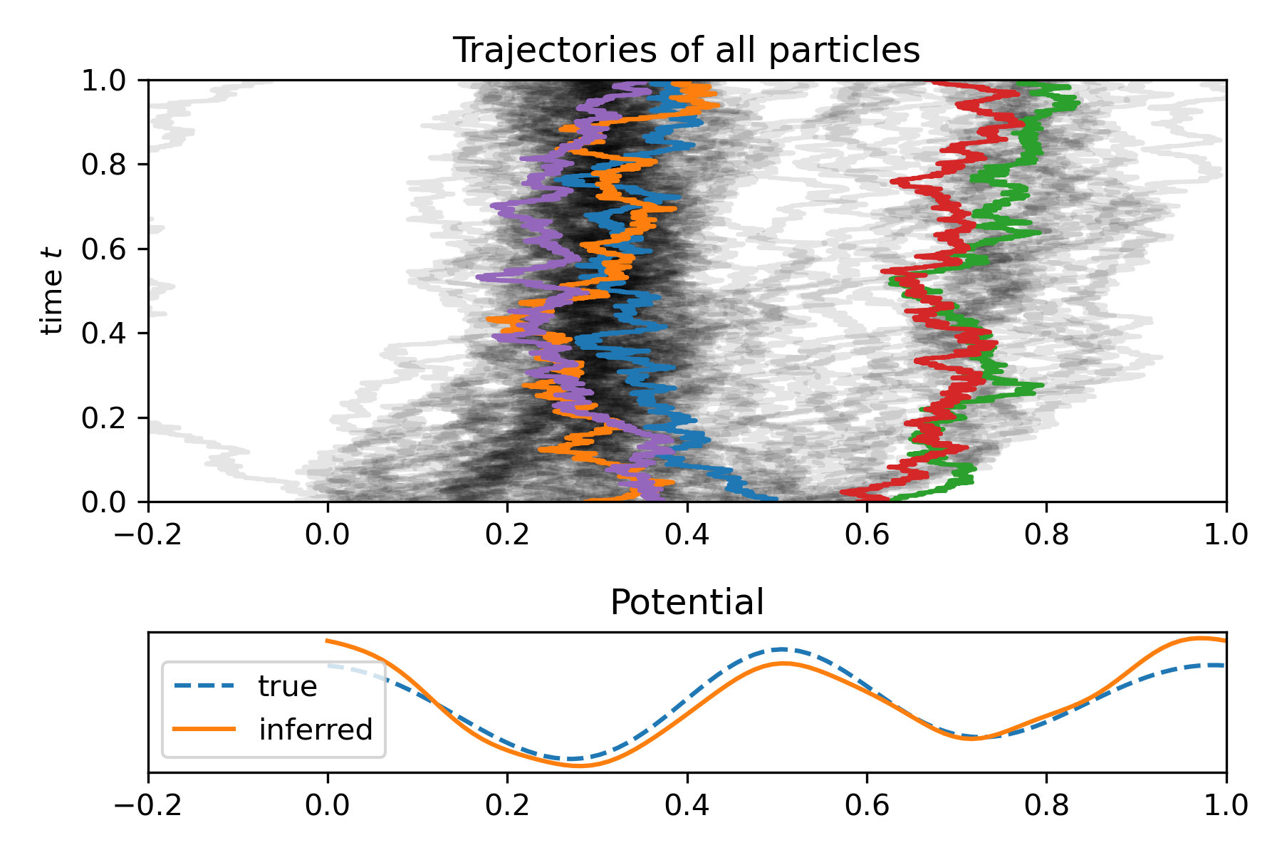
In the following, we perform numerical experiments to empirically validate the existence of a convergence rate in theorem˜5.4 – in fact, we will observe a rate O​(n−1/2)O(n^{-1/2}). For this we perform a series of simulations that model motion of nn particles in a one-dimensional domain Ω\Omega over time t∈[0,1]t\in[0,1]. At the beginning of the simulation for time t=0t=0 the particles are uniformly distributed in [0,1]⊂Ω[0,1]\subset\Omega. Motion of each particle is (independently) governed by the SDE (1), in which we express the drift μ\mu as the superposition of a known spatially constant flux u​(x)=5u(x)=5 and the gradient of a potential Φ:Ω→ℝ\Phi\colon\Omega\rightarrow\mathbb{R},

μ=u+∇Φ\mu=u+\nabla\Phi

(this is allowed since in one space dimension there is a one-to-one relation between potentials and drifts). Our goal in this numerical experiment is to infer the potential Φ\Phi from the observation of motion trajectories of the nn simulated particles.

We use the Euler–Maruyama (EM) method with MM time steps to discretize the SDE in time and track the position of the particles in our simulations. For simplicity, in our simulations we assume that the observation times t0,…,tMt_{0},\ldots,t_{M} coincide with these discretized time steps, i.e. we have a large number of observation times. The EM discretisation provides a direct way of computing the likelihood from one time step to the next. Since we can compute the position qjq_{j} of particle j∈{1,…,n}j\in\{1,\ldots,n\} for the next time step k+1k+1 via

qj(i+1)=qj(i)+Δ​t​μ​(qj(i))+σ​Δ​t​ξ,\displaystyle q_{j}^{(i+1)}=q^{(i)}_{j}+\Delta t\mu(q^{(i)}_{j})+\sigma\sqrt{\Delta t}\xi,

with ξ∼𝒩​(0,1)\xi\sim\mathcal{N}(0,1) normally distributed, we know that for fixed σ\sigma and potential function Φ\Phi it holds

qj(i+1)|qj(i)∼𝒩​(qj(i)+Δ​t​μ​(qj(i)),σ2​Δ​t).\displaystyle\left.q_{j}^{(i+1)}\right|q^{(i)}_{j}\ \sim\ \mathcal{N}\left(q^{(i)}_{j}+\Delta t\mu(q^{(i)}_{j}),\>\sigma^{2}\Delta t\right).

As described in the previous sections, our parameter estimation is based on the fidelity term SτS_{\tau}, the log-likelihood of the observations, shifted by some τ>0\tau>0. In practice, we actually use τ=0\tau=0, i.e. we take SS as our fidelity term. The likelihood of the discrete motion trajectories can practically be calculated by multiplying the above densities for each time step sequentially, using the Markovian property of the underlying SDE and its discretisation. In practice, we directly use the log-likelihood (and summation) to avoid numerical underflow and enable us to evaluate the likelihood for a fixed choice of parameters and a given potential. This approach has the benefit that these parameters and functions can be used within a standard optimisation procedure to infer the potential Φ\Phi from the observed trajectories.

As in the previous sections, we assume σ\sigma to be known. As ground truth Φ†\Phi^{\dagger} of the potential we choose a simple double-well potential, discretised in Fourier space. Naturally, we perform optimisation during inference of Φ\Phi in the space of Fourier modes. Note that in this numerical setup we do not need any additional regularisation since this simple one-dimensional problem is relatively well-posed.

In fig.˜3 we present the results of two particular numerical experiments simulating n=12n=12 (left) and n=120n=120 particles. In the top row we show simulated trajectories for the uniformly distributed particles. The xx-axis shows the respective position qj∈Ωq_{j}\in\Omega of the nn particles, while the yy-axis denotes the time t∈[0,1]t\in[0,1]. Note that for the case n=120n=120 (right) we used shades of grey to accumulate trajectories and highlighted only a few particular trajectories in colour for a better visualization. In the second row we visualize the inferred and true potentials for both numerical experiments. Peaks in the potential lead to repulsion of particles, while valleys in the potential will attract particles. This can already be observed in the simulated trajectories in the top row.

While for the case n=12n=12 (left) the inferred potential (orange curve) loosely follows the characteristics of the ground truth potential (blue curve), the inferred potential in the case n=120n=120 (right) is much closer to the true potential.

Refer to caption
Refer to caption
Figure 3: Left: Simulated trajectories (top) and potential inference (bottom) for n=12n=12 particles. Right: Simulated trajectories (top) and potential inference (bottom) for n=120n=120 particles.

To quantify the error between the inferred potential and the true underlying potential, we performed additional experiments in which the distance is measured in the L2L^{2} norm. In particular, we infer the potential Φ\Phi from the simulated particle trajectories for an increasing amount of particles n=2kn=2^{k}, for k=3,…,10k=3,\ldots,10. To take the stochasticity of the simulations into account, we perform 2525 independent experiments for each amount nn of particles and subsequently compute the mean value and variance of the computed L2L^{2} errors. Figure˜4 shows a box plot of the computed L2L^{2} errors on a logarithmic scale. Additionally, we plot two reference lines for different theoretical rates of convergence: the blue line shows a convergence rate of 𝒪​(n−1/2)\mathcal{O}(n^{-1/2}), while the orange curve shows a convergence rate of 𝒪​(n−1)\mathcal{O}(n^{-1}).

Refer to captionNumber nn of particles

L2L^{2}-norm error


O​(n−1/2)O(n^{-1/2})

O​(n−1)O(n^{-1})

Figure 4: Error between ground truth and inferred potential in L2L^{2} norm, as a function of number of particles tracked, visualised as a box plot over 2525 independent runs each. Asymptotic curves for 𝒪​(n−1/2)\mathcal{O}(n^{-1/2}) and 𝒪​(n−1)\mathcal{O}(n^{-1}) show that convergence is close to 𝒪​(n−1/2)\mathcal{O}(n^{-1/2}).

As can be observed, our numerical experiments exhibit a convergence rate of 𝒪​(n−1/2)\mathcal{O}(n^{-1/2}).

Acknowledgements

This work was supported by the Deutsche Forschungsgemeinschaft (DFG, German Research Foundation) via project 431460824 – Collaborative Research Center 1450 and via Germany’s Excellence Strategy project 390685587 – Mathematics Münster: Dynamics-Geometry-Structure.


References

  • [1] Radu Boţ and Bernd Hofmann. An extension of the variational inequality approach for nonlinear ill-posed problems. 09 2009.
  • [2] J. M. Borwein and A. S. Lewis. Convergence of best entropy estimates. SIAM Journal on Optimization, 1(2):191–205, 1991.
  • [3] Martin Burger and Stanley Osher. Convergence rates of convex variational regularization. Inverse Problems, 20, 07 2004.
  • [4] Fabian Dunker and Thorsten Hohage. On parameter identification in stochastic differential equations by penalized maximum likelihood. Inverse Problems, 30, 08 2014.
  • [5] H Engl, K Kunisch, and A Neubauer. Convergence rates for tikhonov regularisation of non-linear ill-posed problems. Inverse Problems, 5:523, 01 1999.
  • [6] Jens Flemming. Generalized Tikhonov regularization and modern convergence rate theory in Banach spaces. Berichte aus der Mathematik. Shaker Verlag, Aachen, 2012.
  • [7] Jens Flemming and Bernd Hofmann. Convergence rates in constrained Tikhonov regularization: equivalence of projected source conditions and variational inequalities. Inverse Problems, 27(8):085001, 11, 2011.
  • [8] A. Friedman. Partial Differential Equations of Parabolic Type. Dover Books on Mathematics. Dover Publications, 2008.
  • [9] S. Gross-Thebing, L. Truszkowski, D. Tenbrinck, H. Sanchez-Iranzo, C. Camelo, K.J. Westerich, A. Singh, P. Maier, J. Prengel, P. Lange, J. Huewel, F. Gaede, R. Sasse, B.E. Vos, T. Betz, M. Matis, R. Prevedel, S. Luschnig, A. Diz-Munoz, M. Burger, and E. Raz. Using migrating cells as probes to illuminate features in live embryonic tissues. Science Advances, 6(49), 2020.
  • [10] Bernd Hofmann, Barbara Kaltenbacher, Christiane Pöschl, and O Scherzer. A convergence rates result for tikhonov regularization in banach spaces with non-smooth operators. Inverse Problems, 23:987, 04 2007.
  • [11] Bernd Hofmann and Masahiro Yamamoto. On the interplay of source conditions and variational inequalities for nonlinear ill-posed problems. Applicable Analysis, 89:1705–1727, 11 2010.
  • [12] A. M. Il’in, A. S. Kalashnikov, and O. A. Oleinik. Linear equations of the second order of parabolic type. Uspekhi Matematicheskikh Nauk, 17(3):3–146, 1962.
  • [13] Ol’ga A. Ladyženskaja, Vsevolod A. Solonnikov, and Nina N. Ural’ceva. Linear and Quasi-linear Equations of Parabolic Type, volume 23 of Translations of Mathematical Monographs. American Mathematical Society, 1968.
  • [14] Peter Mathé and Bernd Hofmann. How general are general source conditions? Inverse Problems, 24:015009, 01 2008.
  • [15] Christiane Pöschl. Tikhonov Regularization with General Residual Term. PhD thesis, 10 2008.
  • [16] Elena Resmerita and Otmar Scherzer. Error estimates for non-quadratic regularization and the relation to enhancement. Inverse Problems - INVERSE PROBL, 22, 11 2006.
  • [17] Thomas I. Seidman and Curtis R. Vogel. Well-posedness and convergence of some regularisation methods for nonlinear ill posed problems. Inverse Problems, 5(2):227–238, 1989.
  • [18] Frank Werner. Inverse Problems with Poisson Data: Tikhonov-Type Regularization and Iteratively Regularized Newton Methods. PhD thesis, University of Göttingen, Göttingen, Germany, 2012. Doctoral dissertation.
  • [19] Frank Werner and Thorsten Hohage. Convergence rates in expectation for tikhonov-type regularization of inverse problems with poisson data. Inverse Problems, 28, 10 2012.