跳到论文正文
W Papers独立论文阅读器 arXiv:2507.09473 论文正文 计算阅读时间 · 0%
引用这篇论文根据当前论文元数据生成,正式投稿前建议核对。


Incentive-Aware Dynamic Resource Allocation
under Long-Term Cost Constraints

Yan Dai Operations Research Center, MIT. Email: yandai20@mit.edu.    Negin Golrezaei Sloan School of Management, MIT. Email: golrezae@mit.edu.    Patrick Jaillet Department of EECS, MIT. Email: jaillet@mit.edu.
Abstract

Motivated by applications such as cloud platforms allocating GPUs to users or governments deploying mobile health units across competing regions, we study the dynamic allocation of a reusable resource to strategic agents with private valuations. Our objective is to simultaneously (i) maximize social welfare, (ii) satisfy multi-dimensional long-term cost constraints, and (iii) incentivize truthful reporting. We begin by numerically evaluating primal-dual methods widely used in constrained online optimization and find them to be highly fragile in strategic settings – agents can easily manipulate their reports to distort future dual updates for future gain. To address this vulnerability, we develop an incentive-aware framework that makes primal-dual methods robust to strategic behavior. Our design combines epoch-based lazy updates – where dual variables remain fixed within each epoch – with randomized exploration rounds that extract approximately truthful signals for learning. Leveraging carefully designed online learning subroutines that can be of independent interest for dual updates, our mechanism achieves 𝒪~​(T)\widetilde{\mathcal{O}}(\sqrt{T}) social welfare regret, satisfies all cost constraints, and ensures incentive alignment. This matches the performance of non-strategic allocation approaches while being robust to strategic agents.

1 Introduction

Modern platforms and public agencies often face the challenge of allocating limited, reusable resources over time to self-interested agents, who may hide their true desire in sake of more favorable allocations. For example, cloud providers must decide how to distribute scarce GPUs to competing jobs under compute and energy constraints (Buyya et al., 2008, Nejad et al., 2014). Governments may deploy mobile health units or medical devices such as ventilators across regions, where needs vary over time and access is constrained by staffing or capacity (Stummer et al., 2004, Adan et al., 2009). In these settings, a same unit of resource is reallocated across time, and the allocation must respect some multi-dimensional long-term cost constraints – such as energy or staffing – while accounting for the strategic behavior of agents with private information.

A central challenge in these dynamic environments is not only yielding efficient allocations – i.e., maximizing social welfare subject to constraints – but also remain robust to agents’ strategic manipulation. When focusing solely on efficiency, a research problem also known as online resource allocation, the primal-dual method serves as a powerful tool and offers a principled way to handle constraints while adapting to changing demand (Devanur and Hayes, 2009, Golrezaei et al., 2014, Molinaro and Ravi, 2014, Balseiro et al., 2023). These algorithms maintain dual variables that act as shadow prices on resource usage, guiding allocations based on both values and costs. However, these approaches typically assume truthful agents and ignore any strategic responses agents make.

Refer to caption
Figure 1: We simulate a TT-round game for 1000 trials, during which agents use Q-learning to optimize their reporting strategy. Under the vanilla primal-dual algorithm of Balseiro et al. (2023), agents learn to frequently misreport their values, resulting in reduced social welfare and low budget utilization (blue). In contrast, under our incentive-aware mechanism, agents gradually learn to report truthfully, leading to significantly improved social welfare while adhering to cost constraints (green). See Section˜5 for the detailed setup.

Indeed, as we illustrate numerically in Figure˜1, classical primal-dual mechanisms are highly vulnerable to agents’ strategic manipulation: Strategic agents game the learning process by distorting their current reports to influence future dual updates, thereby improving their individual utility at the expense of feasibility and overall efficiency. This fragility raises a natural question:

With strategic agents, is it still possible to optimize social welfare subject to long-term constraints?

To our knowledge, the only prior work addressing strategic agents in online resource allocation is that of Yin et al. (2022). While their framework is a valuable step, it has two key limitations. First, it focuses on homogeneous agents with identical value distributions – an assumption critical for their equilibrium argument, but unrealistic in many applications. Second, their mechanism focuses on a specific type of cost constraint based on some “fair share” per agent, which requires knowing ideal allocation proportions in advance. These assumptions limit the practical applicability of their results. More discussions on it and other related works can be found in Section˜1.1.

In this paper, we go beyond these limitations and propose an incentive-aware mechanism that makes the primal-dual framework robust to strategic manipulation. To limit agents’ ability to influence future dual variables, our mechanism stabilizes dual updates through epoch-based lazy updates, fixing dual variables within each epoch. This design reduces the impact of any individual report on future allocations. To further deter manipulation, we introduce randomized exploration rounds that impose immediate utility loss on untruthful agents, thereby creating localized incentives for truthful reporting. We show that, when adopting a classical Follow-the-Regularized-Leader (FTRL) algorithm for dual updates, our mechanism (i) achieves sublinear regret of 𝒪~​(T2/3)\widetilde{\mathcal{O}}(T^{2/3}) w.r.t. offline optimal allocations, where TT is the number of rounds, (ii) satisfies all resource constraints exactly, and (iii) admits a Perfect Bayesian Equilibrium (PBE) in which agents have no incentives to misreport in most rounds.

We observe that the incentive-compatibility of our mechanism further allows the planner to treat historical agent reports as reliable estimates of true values, thus enabling meaningful predictions of future outcomes. Building on this insight, we introduce a novel online learning algorithm – Optimistic FTRL with Fixed Points (O-FTRL-FP) – which can be of independent interest. By solving a small number of fixed-point problems across the game and incorporating such predictability, it attains an improved 𝒪~⁡(T)\operatorname{\widetilde{\operatorname{\mathcal{O}}}}(\sqrt{T}) regret, matching the Ω​(T)\Omega(\sqrt{T}) lower bound for non-strategic online constrained resource allocations (Arlotto and Gurvich, 2019) in terms of the polynomial dependency on TT. In doing so, we bridge the gap between online constrained optimization and dynamic mechanism design, enabling robust and efficient decision-making in complex, strategic environments.

1.1 Related Work

Dynamic Resource Allocation with Non-Strategic Agents.

With non-strategic agents, dynamic resource allocation, or more generally, online linear programming, was first studied under the random permutation model where an adversary selects a set of requests that are presented in a random order (Devanur and Hayes, 2009, Feldman et al., 2010, Gupta and Molinaro, 2016), which is more general than our i.i.d. model where all values and costs are identically distributed. For the i.i.d. model, various primal-dual-based algorithms were proposed with the main focus of refining computational efficiency (Agrawal et al., 2014, Devanur et al., 2019, Kesselheim et al., 2018, Li et al., 2023); specifically, Li et al. (2023) proposed a fast 𝒪⁡(T1/2)\operatorname{\mathcal{O}}(T^{1/2})-regret algorithm for the online linear programming problem, which matches the Ω​(T1/2)\Omega(T^{1/2}) online resource allocation lower bound (Arlotto and Gurvich, 2019).

Recent progress on this problem includes refined o​(T1/2)o(T^{1/2}) regret under known-distribution assumptions (Sun et al., 2020), or better robustness and adaptivity to adversarial corruptions (Balseiro et al., 2023, Yang et al., 2024). Another closely related problem is Bandits with Knapsacks (BwK), where the planner makes allocations without observing the values or costs in advance but only learns via post-decision feedback (Badanidiyuru et al., 2018, Castiglioni et al., 2022). Nevertheless, none of them considers strategic behaviors of the agents but assume the values and costs are fully truthful. In contrast, our main focus is to be robust to agents’ strategic behaviors while remaining efficient and obeying all the constraints.

Dynamic Resource Allocation with Strategic Agents.

When agents are strategic, ensuring both efficiency and incentive-compatibility provide a foundation for static truthful allocation with monetary transfers. In static (one-shot) allocations when money can be redistributed, the celebrated VCG mechanism (Vickrey, 1961, Clarke, 1971, Groves, 1973) provides a foundation way to achieve both. We study the repeated setup where money can only be charged but not redistributed, the so-called “money-burning” setup. A related problem is learning prices in repeated auctions (Amin et al., 2013; 2014, Kanoria and Nazerzadeh, 2014, Golrezaei et al., 2021a; 2023). These works focus on a seller learning prices to maximize revenue where the agents strategically react to these prices, sometimes subject to buyer’s budget constraints. In our work, we study the different social welfare maximization task and consider more general multi-dimensional cost constraints.

We also briefly discuss the settings where monetary transfers are completely disallowed. In static setups, incentive-compatibility is in general hard due to the Arrow’s impossibility theorem (Arrow, 1950, Gibbard, 1973, Satterthwaite, 1975), though some positive results exist under restricted assumptions (Miralles, 2012, Guo and Conitzer, 2010, Han et al., 2011, Cole et al., 2013). Many recent efforts have been made to ensure efficiency and compatibility in repeated non-monetary allocations, which have very different setups from ours, for example when agents’ value distributions are known (Balseiro et al., 2019, Gorokh et al., 2021b, Blanchard and Jaillet, 2024), when a pre-determined “fair share” is revealed to the planner (Gorokh et al., 2021a, Yin et al., 2022, Banerjee et al., 2023, Fikioris et al., 2023), or when the planner has extra power like audits (Jalota et al., 2024, Dai et al., 2025). We also remark that they either do not consider constraints or only have a specific “fair share” constraint that we discuss later. In contrast, we consider general multi-dimensional constraints.

Multi-Agent Learning.

While our planner learns for better allocation mechanisms, the agents are also learning in reaction to it (e.g., in our numerical illustration in Figure˜1, we consider agents who use Q-learning to learn the best reporting strategies under different dual variables). There is a rich literature investigating this dynamics as well, for example Balseiro and Gur (2019), Golrezaei et al. (2020), Berriaud et al. (2024), Galgana and Golrezaei (2025) studying the convergence to equilibria when multiple agents deploy no-regret online learning algorithms in reaction to some mechanism at the same time. While such results are stronger than our existence of equilibrium results in the sense that agents find such an equilibrium on their own, we remark that the main focus of this work is designing robust mechanisms for the planner instead of designing learning algorithms for the agents.

Comparison with (Yin et al., 2022).

Yin et al. (2022) also study the problem of ensuring efficiency and incentive-compatibility in dynamic constrained resource allocations. The first critical difference is that they assume all the agents have identical value distributions, which is crucial for incentive-compatibility: By comparing one agents’ reports to all the opponents’, unilateral deviation from Truth\operatorname{\textsc{Truth}} is easily caught and thus Truth\operatorname{\textsc{Truth}} is a PBE even without using monetary transfers. In contrast, we need more delicate algorithmic components, including epoch-based lazy updates, random exploration rounds, and dual-adjusted allocation and payment plans, to ensure the near-truthfulness of agents. Another main difference is the type of constraints. They study a specific “fair share” type resource constraint, which says given some 𝒑∈△​([K])\bm{p}\in\triangle([K]), the number of allocations that agent ii receive should be roughly T​piTp_{i}, ∀i∈[K]\forall i\in[K]. In contrast, our multi-dimensional long-term constraint is strictly more general than theirs, which can be written as 1T​∑t=1T𝒆it≤𝒑\frac{1}{T}\sum_{t=1}^{T}\bm{e}_{i_{t}}\leq\bm{p} in our language.

2 Preliminaries

Notations.

For an integer n≥1n\geq 1, [n][n] denotes the set {1,2,…,n}\{1,2,\ldots,n\}. For a set 𝒳\mathcal{X}, the probabilistic simplex △​(𝒳)\triangle(\mathcal{X}) contains all probability distributions over 𝒳\mathcal{X}. We use bold letters like 𝒗\bm{v} to denote a vector, and use normal letters like viv_{i} for an element therein. For a random variable XX, we use PDF(X)\operatornamewithlimits{\mathrm{PDF}}(X) to denote its probability density function (PDF). We use 𝒪\operatorname{\mathcal{O}} to hide all absolute constants, 𝒪~\operatorname{\widetilde{\operatorname{\mathcal{O}}}} to additionally hide all logarithmic factors, and 𝒪~T\operatorname{\widetilde{\operatorname{\mathcal{O}}}}_{T} to focus on the polynomial dependency of TT.

Setup.

We consider the problem of allocating indivisible resources over TT rounds from a central planner to KK strategic agents, indexed by 1,2,…,K1,2,\ldots,K. In each round, the planner allocates a single indivisible resource to one of the agents, aiming to maximize social welfare while satisfying dd long-term cost constraints simultaneously; more details on this objective can be found in Section˜2.3.

2.1 Agents’ Values and Costs, Planner’s Allocation and Payment

In each round t∈[T]t\in[T], agent i∈[K]i\in[K] has a private scalar value vt,i∈[0,1]v_{t,i}\in[0,1] for the resource and a public dd-dimensional cost vector 𝒄t,i∈[0,1]d\bm{c}_{t,i}\in[0,1]^{d}. Allocating the resource to agent ii in round tt yields a value of vt,iv_{t,i} to the agent and incurs ct,i,jc_{t,i,j} units of cost along dimension jj for all j∈[d]j\in[d]. We assume that values and costs are independently generated across agents and rounds; specifically, vt,iv_{t,i} and 𝒄t,i\bm{c}_{t,i} are i.i.d. samples from some fixed but unknown distributions 𝒱i∈△​([0,1])\mathcal{V}_{i}\in\triangle([0,1]) and 𝒞i∈△​([0,1]d)\mathcal{C}_{i}\in\triangle([0,1]^{d}), respectively, for all t∈[T]t\in[T] and i∈[K]i\in[K].

Every agent i∈[K]i\in[K], after observing their own private value vt,iv_{t,i}, strategically generates a report ut,i∈[0,1]u_{t,i}\in[0,1] which may differ from vt,iv_{t,i}. We defer the generation rule of such reports to Section˜2.2. After observing agents’ strategic reports 𝒖t\bm{u}_{t} and cost vectors 𝒄t\bm{c}_{t} (but without access to the true values 𝒗t\bm{v}_{t}), the planner either irrevocably allocates the resource to one of the agents it∈[K]i_{t}\in[K] or forfeits it for this round, in which case we write it=0i_{t}=0. Conventionally, vt,0=0v_{t,0}=0 and 𝒄t,0=𝟎\bm{c}_{t,0}=\bm{0} for all t∈[T]t\in[T].

After the allocation, the planner decides a payment charged from the winner iti_{t}, denoted by pt,itp_{t,i_{t}}. For all remaining agents i≠iti\neq i_{t}, the payment pt,i=0p_{t,i}=0. The planner maximizes the TT-round cumulative social welfare ∑t=1Tvt,it\sum_{t=1}^{T}v_{t,i_{t}} subject to long-term constraints that the TT-round average costs are no more than a pre-specified threshold 𝝆∈[0,1]d\bm{\rho}\in[0,1]^{d}, i.e., 1T​∑t=1T𝒄t,it≤𝝆\frac{1}{T}\sum_{t=1}^{T}\bm{c}_{t,i_{t}}\leq\bm{\rho}, where ≤\leq is compared element-wise.

Protocol 1 Interaction Protocol for Repeated Resource Allocation

protocol]alg:protocol

Number of rounds TT, number of agents KK, value distributions {𝒱i}i∈[K]\{\mathcal{V}_{i}\}_{i\in[K]}, cost distributions {𝒞i}i∈[K]\{\mathcal{C}_{i}\}_{i\in[K]}, mechanism 𝑴=(Mt)t∈[T]\bm{M}=(M_{t})_{t\in[T]}, agents’ strategy profile 𝝅=(πt,i)t∈[T],i∈[K]\bm{\pi}=(\pi_{t,i})_{t\in[T],\,i\in[K]}
1:Initialize public history: ℋ1,0←∅\mathcal{H}_{1,0}\leftarrow\varnothing
2:Initialize private history for each agent ii: ℋ1,i←{(𝒱j,𝒞j)}j∈[K]\mathcal{H}_{1,i}\leftarrow\{(\mathcal{V}_{j},\mathcal{C}_{j})\}_{j\in[K]} \Foreach round t=1,2,…,Tt=1,2,\dots,T
3:Each agent i∈[K]i\in[K] observes:
  • •

    Private value: vt,i∼𝒱iv_{t,i}\sim\mathcal{V}_{i}

  • •

    Public cost vector: 𝒄t,i∼𝒞i\bm{c}_{t,i}\sim\mathcal{C}_{i}

4:Agent ii submits report: ut,i∼πt,i​(vt,i,𝒄t;ℋt,i)u_{t,i}\sim\pi_{t,i}(v_{t,i},\bm{c}_{t};\mathcal{H}_{t,i})
5:Planner applies mechanism: (it,pt,it)∼Mt​(𝒖t,𝒄t;ℋt,0)(i_{t},p_{t,i_{t}})\sim M_{t}(\bm{u}_{t},\bm{c}_{t};\mathcal{H}_{t,0})
6:Update public history: add (𝒖t,𝒄t,it,pt,it)(\bm{u}_{t},\bm{c}_{t},i_{t},p_{t,i_{t}}) to ℋt+1,0\mathcal{H}_{t+1,0}
7:Each agent ii updates private history: add vt,iv_{t,i} and (𝒖t,𝒄t,it,pt,it)(\bm{u}_{t},\bm{c}_{t},i_{t},p_{t,i_{t}}) to ℋt+1,i\mathcal{H}_{t+1,i} \EndFor
\Require

2.2 History, Planner’s Mechanism, and Agents’ Strategies

At the beginning of round t∈[T]t\in[T], the public history that is available to all participants (i.e., the planner and all agents) includes all previous reports, costs, allocations, and payments; we denote the public history in round tt by ℋt,0:={(𝒖τ,𝒄τ,iτ,pτ,iτ)}τ<t\mathcal{H}_{t,0}:=\{(\bm{u}_{\tau},\bm{c}_{\tau},i_{\tau},p_{\tau,i_{\tau}})\}_{\tau<t}. Each agent i∈[K]i\in[K] additionally has access to their own past values and all agents’ value and cost distributions. Thus, the private history available to agent i∈[K]i\in[K] at the beginning of round t∈[T]t\in[T] is 111We assume the distributional information is known across the agents since such information (or at least some prior) is necessary for the definition of Perfect Bayesian Equilibrium (PBE) in Definition 2. We adopt this mutually known setup as it is most challenging for the planner in terms of information asymmetry.

ℋt,i:=ℋt,0∪{vτ,i}τ<t∪{(𝒱j,𝒞j)}j∈[K].\mathcal{H}_{t,i}:=\mathcal{H}_{t,0}\cup\{v_{\tau,i}\}_{\tau<t}\cup\{(\mathcal{V}_{j},\mathcal{C}_{j})\}_{j\in[K]}.

In each round t∈[T]t\in[T], the planner determines the allocation and payment (it,pt,it)(i_{t},p_{t,i_{t}}) based on agents’ reports 𝒖t\bm{u}_{t}, cost vectors 𝒄t\bm{c}_{t}, public history ℋt,0\mathcal{H}_{t,0}, and possibly some internal randomness used to break ties or randomize decisions. We write it=pt,it=0i_{t}=p_{t,i_{t}}=0 when the allocation is forfeited. We remark that the payment is allowed to be both positive or negative. Formally,

(it,pt,it)∼Mt​(𝒖t,𝒄t;ℋt,0),where ​Mt:(𝒖t,𝒄t,ℋt,0)↦PDF(it,pt,it).\displaystyle(i_{t},p_{t,i_{t}})\sim M_{t}(\bm{u}_{t},\bm{c}_{t};\mathcal{H}_{t,0}),\quad\text{where }M_{t}\colon(\bm{u}_{t},\bm{c}_{t},\mathcal{H}_{t,0})\mapsto\operatornamewithlimits{\mathrm{PDF}}(i_{t},p_{t,i_{t}}).

The collection of decision rules 𝑴=(Mt)t∈[T]\bm{M}=(M_{t})_{t\in[T]} is referred to as the planner’s mechanism. We emphasize that the planner does not know the agents’ value or cost distributions, whereas the mechanism 𝑴\bm{M} is publicly known to the agents, as is standard in the literature.

For each agent i∈[K]i\in[K], their report ut,iu_{t,i} is determined based on their private value vt,iv_{t,i}, the cost vector 𝒄t\bm{c}_{t}, their private history ℋt,i\mathcal{H}_{t,i}, and potentially some internal randomness. Formally, we write

ut,i∼πt,i​(vt,i,𝒄t;ℋt,i),where ​πt,i:(vt,i,𝒄t,ℋt,i)↦PDF(ut,i).\displaystyle u_{t,i}\sim\pi_{t,i}(v_{t,i},\bm{c}_{t};\mathcal{H}_{t,i}),\quad\text{where }\pi_{t,i}\colon(v_{t,i},\bm{c}_{t},\mathcal{H}_{t,i})\mapsto\operatornamewithlimits{\mathrm{PDF}}(u_{t,i}).

Agent ii’s decision rules collectively form their strategy 𝝅i:=(πt,i)t∈[T]\bm{\pi}_{i}:=(\pi_{t,i})_{t\in[T]}. The agents’ strategies together constitute a joint strategy 𝝅:=(𝝅i)i∈[K]\bm{\pi}:=(\bm{\pi}_{i})_{i\in[K]}. We summarize the interaction as LABEL:alg:protocol.

2.3 Agents’ Behavior and Planner’s Regret

To model agents’ behavior in a dynamic environment, we adopt the γ\gamma-impatient agent model by Golrezaei et al. (2021a; 2023), which captures the idea that agents often prioritize immediate rewards over long-term gains – due to bounded rationality, uncertainty about future rounds, or limited planning horizons – while the planner is more patiently optimizing the long-run welfare.

Assumption 1 (γ\gamma-Impatient Agents).

For some fixed but unknown constant γ∈(0,1)\gamma\in(0,1), every agent i∈[K]i\in[K] is γ\gamma-impatient in the sense that they maximize their γ\gamma-discounted TT-round gain 222Two special cases of Assumption 1 are 0-impatient agents, who only care about their gains in the current round (often referred to as myopic agent), and 11-impatient agents, who care about their total gains over the entire TT-round game (as is typical in extensive-form games).

Viγ​(𝝅;𝑴):=𝔼LABEL:alg:protocol[∑t=1Tγt​(vt,i−pt,i)​𝟙​[it=i]],∀i∈[K],agents’ strategy ​𝝅,mechanism ​𝑴.\displaystyle V_{i}^{\gamma}(\bm{\pi};\bm{M}):=\operatornamewithlimits{\mathbb{E}}_{\text{\lx@cref{creftypecap~refnum}{alg:protocol}}}\left[\sum_{t=1}^{T}\gamma^{t}(v_{t,i}-p_{t,i})\mathbbm{1}[i_{t}=i]\right],\quad\forall i\in[K],\text{agents' strategy }\bm{\pi},\text{mechanism }\bm{M}. (1)

In this paper, we study the equilibrium concept of Perfect Bayesian Equilibrium (PBE):

Definition 2 (Perfect Bayesian Equilibrium).

Fix mechanism 𝐌=(M1,M2,…,MT)\bm{M}=(M_{1},M_{2},\ldots,M_{T}). An agents’ joint strategy 𝛑\bm{\pi} is a Perfect Bayesian Equilibrium (PBE) under 𝐌\bm{M}, if any single agent’s unilateral deviation from 𝛑\bm{\pi} does not increase their own gain. Formally, joint strategy 𝛑\bm{\pi} is a PBE if

Viγ​(𝝅i∘𝝅−i;𝑴)≥Viγ​(𝝅i′∘𝝅−i;𝑴),∀i∈[K],∀agent i’s strategy ​𝝅i′.\displaystyle V_{i}^{\gamma}(\bm{\pi}_{i}\circ\bm{\pi}_{-i};\bm{M})\geq V_{i}^{\gamma}(\bm{\pi}_{i}^{\prime}\circ\bm{\pi}_{-i};\bm{M}),\quad\forall i\in[K],\forall\text{agent $i$'s strategy }\bm{\pi}_{i}^{\prime}.

The planner aims to maximize the non-discounted social welfare, namely the expected total value yielded from allocations 𝔼[∑t=1Tvt,it]\operatornamewithlimits{\mathbb{E}}[\sum_{t=1}^{T}v_{t,i_{t}}], while satisfying the dd long-term cost constraints 1T​∑t=1T𝒄t,it≤𝝆\frac{1}{T}\sum_{t=1}^{T}\bm{c}_{t,i_{t}}\leq\bm{\rho} simultaneously. To evaluate a mechanism’s performance, we compare the allocations against the following offline optimal benchmark, which performs a hindsight optimization using agents’ true values and costs:

{it∗}t∈[T]:=argmaxi1∗,…,iT∗∈{0}∪[K]​∑t=1Tvt,it∗subject to1T​∑t=1T𝒄t,it∗≤𝝆.\displaystyle\{i_{t}^{\ast}\}_{t\in[T]}:=\operatornamewithlimits{\mathrm{argmax}}_{i_{1}^{\ast},\ldots,i_{T}^{\ast}\in\{0\}\cup[K]}\sum_{t=1}^{T}v_{t,i_{t}^{\ast}}\quad\text{subject to}\quad\frac{1}{T}\sum_{t=1}^{T}\bm{c}_{t,i_{t}^{\ast}}\leq\bm{\rho}. (2)

We remark that benchmark in Equation˜2 depends on the full sequence of true values {𝒗t}t=1T\{\bm{v}_{t}\}_{t=1}^{T} and costs {𝒄t}t=1T\{\bm{c}_{t}\}_{t=1}^{T}, which are (i) not finalized until the end of the game, and (ii) not fully observable to the planner. This distinguishes it from typical online learning benchmarks, which fixes a policy before the game; see (Balseiro et al., 2023) for a related discussion. Since Equation˜2 relies on information unavailable at decision time, it cannot be matched exactly. Instead, we assess the mechanism’s performance by measuring its regret relative to the offline optimal:

ℜT​(𝝅,𝑴):=𝔼LABEL:alg:protocol[∑t=1T(vt,it∗−vt,it)],\mathfrak{R}_{T}(\bm{\pi},\bm{M}):=\operatornamewithlimits{\mathbb{E}}_{\text{\lx@cref{creftypecap~refnum}{alg:protocol}}}\left[\sum_{t=1}^{T}\left(v_{t,i_{t}^{\ast}}-v_{t,i_{t}}\right)\right], (3)

where the expectation is over the randomness in the mechanism, agent strategies, and value/cost realizations. This regret notion generalizes the one studied in the non-strategic setting of Balseiro et al. (2023), where agents report truthfully (i.e., 𝝅=Truth\bm{\pi}=\operatorname{\textsc{Truth}} such that ut,i=vt,iu_{t,i}=v_{t,i} for all tt and ii). In that setting, their mechanism 𝑴0\bm{M}^{0} achieved regret ℜT​(Truth,𝑴0)=𝒪~⁡(T)\mathfrak{R}_{T}(\operatorname{\textsc{Truth}},\bm{M}^{0})=\operatorname{\widetilde{\operatorname{\mathcal{O}}}}(\sqrt{T}). However, if agents are strategic, they may deviate from truthful reporting. In contrast, our mechanism in Algorithm˜2 guarantees the existence of a Perfect Bayesian Equilibrium (PBE) strategy profile 𝝅\bm{\pi} such that no agent benefits from unilateral deviation, and under which the regret remains 𝒪~⁡(T)\operatorname{\widetilde{\operatorname{\mathcal{O}}}}(\sqrt{T}) (Theorem˜3.2).

In parallel, the planner also aims to minimize constraint violations, which we define as

𝔅T​(𝝅,𝑴):=𝔼LABEL:alg:protocol[∥(∑t=1T(𝒄t,it−𝝆))+∥1],\mathfrak{B}_{T}(\bm{\pi},\bm{M}):=\operatornamewithlimits{\mathbb{E}}_{\text{\lx@cref{creftypecap~refnum}{alg:protocol}}}\Big{[}\big{\lVert}\big{(}\sum_{t=1}^{T}(\bm{c}_{t,i_{t}}-\bm{\rho})\big{)}_{+}\big{\rVert}_{1}\Big{]}, (4)

where (⋅)+(\cdot)_{+} is the coordinate-wise maximum with zero, i.e., 𝒙+:=[max⁡(xi,0)]i∈[d]\bm{x}_{+}:=[\max(x_{i},0)]_{i\in[d]}. Our mechanism 𝑴\bm{M}, presented in Algorithm˜2, guarantees 𝔅T​(𝝅,𝑴)=0\mathfrak{B}_{T}(\bm{\pi},\bm{M})=0; that is, cost constraints are satisfied.

We conclude this section with a smoothness assumption on cost distributions. The idea is to ensure that projected costs (linear combinations of the cost vector) do not place excessive probability mass on any single value. This smoothness condition prevents pathological behaviors where a small change in an agent’s report could drastically alter outcomes due to spiky distributions. Such assumptions are common in strategic settings to ensure robustness to perturbations, including in bilateral trades (Cesa-Bianchi et al., 2024a), first-price auctions (Cesa-Bianchi et al., 2024b), second-price auctions with reserves (Golrezaei et al., 2021a), and smoothed revenue maximization (Durvasula et al., 2023).

Assumption 3 (Smooth Costs).

For any agent i∈[K]i\in[K], the cost distribution 𝒞i\mathcal{C}_{i} satisfies the following: for all 𝛌∈𝚲:={𝛌∈ℝd∣λj∈[0,ρj−1]}\bm{\lambda}\in\bm{\Lambda}:=\{\bm{\lambda}\in\mathbb{R}^{d}\mid\lambda_{j}\in[0,\rho_{j}^{-1}]\}, the density of the projected cost PDF𝐜t∼𝒞i(𝛌⊤​𝐜i){\operatornamewithlimits{\mathrm{PDF}}}_{\bm{c}_{t}\sim\mathcal{C}_{i}}(\bm{\lambda}^{\top}\bm{c}_{i}) is uniformly bounded above by some universal constant ϵc>0\epsilon_{c}>0.

Similar to the γ\gamma in Assumption˜1, we do not assume this ϵc\epsilon_{c} to be known a-priori to the planner.

3 Primal-Dual Mechanism Robust to Strategic Manipulation

Our incentive-aware resource allocation mechanism can be divided into two components, an incentive-aware primal allocation framework which discourages agents’ strategic behaviors, and an online-learning–based dual update rule that is robust to agents’ misreports. We describe the main algorithmic components below before presenting the pseudo-codes and guarantees.

Algorithm 2 Incentive-Aware Primal Allocation Framework Robust to Strategic Manipulations
Number of rounds TT, agents KK, resources dd, cost constraint 𝝆∈[0,1]d\bm{\rho}\in[0,1]^{d}
1:Epochs {ℰℓ}ℓ=1L\{\mathcal{E}_{\ell}\}_{\ell=1}^{L}, learning rates {ηℓ}ℓ=1L\{\eta_{\ell}\}_{\ell=1}^{L}, regularizer Ψ:ℝ≥0d→ℝ\Psi\colon\mathbb{R}_{\geq 0}^{d}\to\mathbb{R}, sub-routine 𝒜\mathcal{A} \EnsureAllocations i1,…,iTi_{1},\ldots,i_{T}, where it=0i_{t}=0 denotes no allocation
2:Define dual region 𝚲:={𝝀∈ℝd:λj∈[0,ρj−1]}\bm{\Lambda}:=\{\bm{\lambda}\in\mathbb{R}^{d}:\lambda_{j}\in[0,\rho_{j}^{-1}]\} \Forepoch ℓ=1,2,…,L\ell=1,2,\ldots,L
3:Update dual variable 𝝀ℓ∈𝚲\bm{\lambda}_{\ell}\in\bm{\Lambda} via the sub-routine 𝒜\mathcal{A}: 𝝀ℓ←𝒜​(ℓ,ηℓ,Ψ)\bm{\lambda}_{\ell}\leftarrow\mathcal{A}(\ell,\eta_{\ell},\Psi). \Foreach round t∈ℰℓt\in\mathcal{E}_{\ell}
4:Each agent i∈[K]i\in[K] observes their value vt,i∼𝒱iv_{t,i}\sim\mathcal{V}_{i} and costs 𝒄t∼𝒞\bm{c}_{t}\sim\mathcal{C}
5:Agent reports ut,i∈[0,1]u_{t,i}\in[0,1] according to LABEL:alg:protocol; 𝒖t\bm{u}_{t} and 𝒄t\bm{c}_{t} become public. \Ifround tt is selected for exploration (w.p. 1/|ℰℓ|1/|\mathcal{E}_{\ell}| independently)
6:Sample tentative agent i∼Unif​([K])i\sim\text{Unif}([K]) and payment p∼Unif​([0,1])p\sim\text{Unif}([0,1])
7:If ut,i≥pu_{t,i}\geq p, set it=ii_{t}=i and pt,it=pp_{t,i_{t}}=p. Otherwise, set it=0i_{t}=0 \Else
8:Compute adjusted cost c~t,i=𝝀ℓ⊤​𝒄t,i\widetilde{c}_{t,i}=\bm{\lambda}_{\ell}^{\top}\bm{c}_{t,i} and adjusted report u~t,i:=ut,i−c~t,i\widetilde{u}_{t,i}:=u_{t,i}-\widetilde{c}_{t,i}, ∀i∈[K]\forall i\in[K]
9:Allocate to agent it:=arg⁡maxi⁡u~t,ii_{t}:=\arg\max_{i}\widetilde{u}_{t,i} with payment pt,it=c~t,it+maxj≠it⁡u~t,jp_{t,i_{t}}=\widetilde{c}_{t,i_{t}}+\max_{j\neq i_{t}}\widetilde{u}_{t,j} \EndIf\Ifcost constraint is violated: ∑s<t𝒄s,is+𝒄t,it≰T​𝝆\sum_{s<t}\bm{c}_{s,i_{s}}+\bm{c}_{t,i_{t}}\not\leq T\bm{\rho}
10:Reject allocation by setting it=0i_{t}=0 \EndIf\EndFor\EndFor
\Require

3.1 Incentive-Aware Primal Allocation Framework

We introduce our incentive-aware primal allocation framework in Algorithm˜2. As numerically illustrated in Figure˜1, vanilla primal-dual methods allow agents to manipulate future dual updates by misreporting, leading to misaligned incentives and degraded performance; see also Example˜4 for a concrete case. Our framework addresses this challenge through three key innovations: epoch-based lazy dual updates, dual-adjusted allocation and payments, and randomized exploration rounds.

Epoch-Based Lazy Updates.

To overcome the vulnerability of vanilla primal-dual methods to strategic behaviors, which is largely due to frequent dual updates, we divide the game horizon [T][T] into LL epochs as [T]=ℰ1∪⋯∪ℰL[T]=\mathcal{E}_{1}\cup\cdots\cup\mathcal{E}_{L} and fix a single dual variable 𝝀ℓ\bm{\lambda}_{\ell} within each epoch ℰℓ\mathcal{E}_{\ell}. As in the standard primal-dual methods, these dual variables act as implicit prices on resource consumption and we adjust reported values accordingly. By additionally holding 𝝀ℓ\bm{\lambda}_{\ell} constant within each epoch, we reduce agents’ ability and willingness to manipulate future allocations through misreports. This “lazy update” scheme is a central ingredient in limiting intertemporal strategic behavior; we refer the readers to Theorem˜4.2 for more details.

Dual-Adjusted Allocation and Payments.

In each round t∈[T]t\in[T], agents submit reports based on their private values and observed costs. With high probability, the mechanism enters a standard round, allocating the resource to the agent with the highest dual-adjusted report (reported value minus dual-weighted cost, i.e., ut,i−𝝀t𝖳​𝒄t,iu_{t,i}-\bm{\lambda}_{t}^{\mathsf{T}}\bm{c}_{t,i}), and charging them their cost plus the second-highest dual-adjusted report – as illustrated in Line˜9 of Algorithm˜2. This payment rule, inspired by boosted second-price auctions (Golrezaei et al., 2021b), is incentive-compatible in static (one-shot) settings and encourages truthful reporting in our dynamic setup; see Theorem˜4.1 from Section˜4.1. If the allocation would violate the cumulative cost constraint, it is rejected to ensure feasibility.

Randomized Exploration Rounds.

With a small probability, the mechanism initiates an exploration round, offering a random price to a randomly selected agent. This structure penalizes misreports by imposing an immediate utility loss when the reported value deviates from the true value. These rounds act as incentive-compatible signal extractors and are essential for maintaining the accuracy of dual updates based on strategic reports. The idea of randomized pricing has been explored in repeated second-price auctions (Amin et al., 2013, Golrezaei et al., 2021a; 2023). But to our knowledge, our work is the first to leverage it for robust primal-dual learning.

3.2 Dual Updates via Online Learning

In the beginning of each epoch ℰℓ\mathcal{E}_{\ell}, the planner decides the dual variable 𝝀ℓ\bm{\lambda}_{\ell}, which we formulate as an online learning problem (see Lemma˜4.3), with past constraint violations as observed losses. In Theorem˜3.1, we show the classical Follow-the-Regularized-Leader (FTRL) method in Equation˜5 achieves 𝒪~⁡(T2/3)\operatorname{\widetilde{\operatorname{\mathcal{O}}}}(T^{2/3}) regret. However, this seems to the best one can hope – while epoch-based lazy updates suppress agents’ incentives to manipulate their reports, they also make dual updates less accurate and impose an Ω​(T2/3)\Omega(T^{2/3}) barrier for most online learning algorithms, as shown in Theorem˜4.4.

To go beyond the 𝒪~​(T2/3)\widetilde{\mathcal{O}}(T^{2/3}) regret of FTRL, we leverage the near-truthfulness induced by our primal allocation framework: Since agents were mostly truthful in the past and will continue to be near-truthful in the future, we can predict their future behavior based on historical information. Our Optimistic FTRL with Fixed Points (O-FTRL-FP) method, as illustrated in Equation˜6, augments classical FTRL with a forward-looking term that estimates how the current dual variable 𝝀ℓ\bm{\lambda}_{\ell} would perform if agent behavior remains consistent.

Specifically, O-FTRL-FP solves a fixed-point problem: It chooses the new dual variable 𝝀ℓ∈𝚲\bm{\lambda}_{\ell}\in\bm{\Lambda} that is at the same time a minimizer 𝝀∈𝚲\bm{\lambda}\in\bm{\Lambda} of the sum of (i) cumulative losses due to past constraint violations ∑τ(𝝆−𝒄τ,iτ)𝖳​𝝀\sum_{\tau}(\bm{\rho}-\bm{c}_{\tau,i_{\tau}})^{\mathsf{T}}\bm{\lambda}, (ii) an optimistic prediction function 𝒈~ℓ​(𝝀ℓ)𝖳​𝝀\widetilde{\bm{g}}_{\ell}(\bm{\lambda}_{\ell})^{\mathsf{T}}\bm{\lambda} that estimates how the new choice of 𝝀ℓ\bm{\lambda}_{\ell} would perform if agents kept their historical behaviors, and (iii) a regularization function Ψ​(𝝀)ηℓ\frac{\Psi(\bm{\lambda})}{\eta_{\ell}}. Since 𝒈~ℓ​(𝝀ℓ)\widetilde{\bm{g}}_{\ell}(\bm{\lambda}_{\ell}) itself depends on 𝝀ℓ\bm{\lambda}_{\ell}, the optimization forms a self-consistent loop. We discuss the existence of (approximate) fixed points in Section˜4.2 and a computationally more efficient approximation in Section˜5. In Theorem˜3.2, we show that this method achieves 𝒪~​(T)\widetilde{\mathcal{O}}(\sqrt{T}) regret while maintaining feasibility and incentive alignment.

Algorithm 3 Dual Update Sub-Routine using Follow-the-Regularized-Leader (FTRL)
Current epoch number ℓ\ell, learning rate ηℓ>0\eta_{\ell}>0, regularizer Ψ:ℝ≥0d→ℝ\Psi\colon\mathbb{R}_{\geq 0}^{d}\to\mathbb{R}
1:Solve the following optimization problem for 𝝀ℓ∈𝚲\bm{\lambda}_{\ell}\in\bm{\Lambda} and return 𝝀ℓ\bm{\lambda}_{\ell}.
𝝀ℓ\displaystyle\bm{\lambda}_{\ell} =argmin𝝀∈𝚲​∑ℓ′<ℓ∑τ∈ℰℓ′(𝝆−𝒄τ,iτ)𝖳​𝝀+1ηℓ​Ψ​(𝝀).\displaystyle=\operatornamewithlimits{\mathrm{argmin}}_{\bm{\lambda}\in\bm{\Lambda}}\sum_{\ell^{\prime}<\ell}\sum_{\tau\in\mathcal{E}_{\ell^{\prime}}}(\bm{\rho}-\bm{c}_{\tau,i_{\tau}})^{\mathsf{T}}\bm{\lambda}+\frac{1}{\eta_{\ell}}\Psi(\bm{\lambda}). (5)
\Require
Algorithm 4 Dual Update Sub-Routine using Optimistic FTRL with Fixed Points (O-FTRL-FP)
Current epoch number ℓ\ell, learning rate ηℓ>0\eta_{\ell}>0, regularizer Ψ:ℝ≥0d→ℝ\Psi\colon\mathbb{R}_{\geq 0}^{d}\to\mathbb{R}
1:Solve the following fixed point problem for (𝝀ℓ,𝒈~ℓ)∈𝚲×ℝd(\bm{\lambda}_{\ell},\widetilde{\bm{g}}_{\ell})\in\bm{\Lambda}\times\mathbb{R}^{d} and return 𝝀ℓ\bm{\lambda}_{\ell}.
𝝀ℓ\displaystyle\bm{\lambda}_{\ell} =argmin𝝀∈𝚲​∑ℓ′<ℓ∑τ∈ℰℓ′(𝝆−𝒄τ,iτ)𝖳​𝝀+𝒈~ℓ​(𝝀ℓ)𝖳​𝝀+1ηℓ​Ψ​(𝝀),\displaystyle=\operatornamewithlimits{\mathrm{argmin}}_{\bm{\lambda}\in\bm{\Lambda}}\sum_{\ell^{\prime}<\ell}\sum_{\tau\in\mathcal{E}_{\ell^{\prime}}}(\bm{\rho}-\bm{c}_{\tau,i_{\tau}})^{\mathsf{T}}\bm{\lambda}+\widetilde{\bm{g}}_{\ell}(\bm{\lambda}_{\ell})^{\mathsf{T}}\bm{\lambda}+\frac{1}{\eta_{\ell}}\Psi(\bm{\lambda}),
𝒈~ℓ​(𝝀ℓ)\displaystyle\widetilde{\bm{g}}_{\ell}(\bm{\lambda}_{\ell}) :=|ℰℓ|⋅1∑ℓ′<ℓ|ℰℓ′|​∑ℓ′<ℓ,τ∈ℰℓ′(𝝆−𝒄τ,i~τ​(𝝀ℓ)),\displaystyle:=\lvert\mathcal{E}_{\ell}\rvert\cdot\frac{1}{\sum_{\ell^{\prime}<\ell}\lvert\mathcal{E}_{\ell^{\prime}}\rvert}\sum_{\ell^{\prime}<\ell,\tau\in\mathcal{E}_{\ell^{\prime}}}\left(\bm{\rho}-\bm{c}_{\tau,\widetilde{i}_{\tau}(\bm{\lambda}_{\ell})}\right),
i~τ​(𝝀ℓ)\displaystyle\widetilde{i}_{\tau}(\bm{\lambda}_{\ell}) :=argmaxi∈{0}∪[K](uτ,i−𝝀ℓ𝖳​𝒄τ,i),∀ℓ′<ℓ,τ∈ℰℓ′.\displaystyle:=\operatornamewithlimits{\mathrm{argmax}}_{i\in\{0\}\cup[K]}\left(u_{\tau,i}-\bm{\lambda}_{\ell}^{\mathsf{T}}\bm{c}_{\tau,i}\right),\quad\forall\ell^{\prime}<\ell,\tau\in\mathcal{E}_{\ell^{\prime}}. (6)
\Require

3.3 Main Results

We now state our two main guarantees, corresponding to different dual update rules. Formal statements and proofs are provided in Appendix˜A, and we highlight the key analyses in Section˜4.

Theorem 3.1 (Algorithm˜2 with FTRL).

Under appropriate choice of epoch lengths and learning rates, Algorithm˜2 using FTRL in Equation˜5 as the dual-update sub-routine 𝒜\mathcal{A} guarantees the existence of a PBE 𝛑∗\bm{\pi}^{\ast} such that ℛT​(𝛑∗,Algorithm˜2)=𝒪~​(T2/3)\mathcal{R}_{T}(\bm{\pi}^{\ast},\text{\lx@cref{creftypecap~refnum}{alg:mech}})=\widetilde{\mathcal{O}}(T^{2/3}) and ℬT​(𝛑∗,Algorithm˜2)=0\mathcal{B}_{T}(\bm{\pi}^{\ast},\text{\lx@cref{creftypecap~refnum}{alg:mech}})=0.

Theorem 3.2 (Algorithm˜2 with O-FTRL-FP).

Under appropriate choice of epoch lengths and learning rates, Algorithm˜2 using O-FTRL-FP in Equation˜6 as the dual-update sub-routine 𝒜\mathcal{A} guarantees the existence of a PBE 𝛑∗\bm{\pi}^{\ast} such that ℛT​(𝛑∗,Algorithm˜2)=𝒪~​(T)\mathcal{R}_{T}(\bm{\pi}^{\ast},\text{\lx@cref{creftypecap~refnum}{alg:mech}})=\widetilde{\mathcal{O}}(\sqrt{T}) and ℬT​(𝛑∗,Algorithm˜2)=0\mathcal{B}_{T}(\bm{\pi}^{\ast},\text{\lx@cref{creftypecap~refnum}{alg:mech}})=0.

4 Analysis Sketch of Theorems˜3.1 and 3.2

The safety property of Algorithm˜2, namely that 𝔅T=0\mathfrak{B}_{T}=0, follows directly from Line˜10. Thus, we focus on analyzing the regret ℜT=𝔼​[∑t=1T(vt,it∗−vt,it)]\mathfrak{R}_{T}=\mathbb{E}\big{[}\sum_{t=1}^{T}(v_{t,i_{t}^{\ast}}-v_{t,i_{t}})\big{]}, which measures the expected difference between our allocation {it}t∈[T]\{i_{t}\}_{t\in[T]} and the offline optimal allocation {it∗}t∈[T]\{i_{t}^{\ast}\}_{t\in[T]} defined in Equation˜2:

{it∗}t∈[T]=argmaxi1∗,…,iT∗∈{0}∪[K]​∑t=1Tvt,it∗subject to1T​∑t=1T𝒄t,it∗≤𝝆.\{i_{t}^{\ast}\}_{t\in[T]}=\operatornamewithlimits{\mathrm{argmax}}_{i_{1}^{\ast},\ldots,i_{T}^{\ast}\in\{0\}\cup[K]}\sum_{t=1}^{T}v_{t,i_{t}^{\ast}}\quad\text{subject to}\quad\frac{1}{T}\sum_{t=1}^{T}\bm{c}_{t,i_{t}^{\ast}}\leq\bm{\rho}.

To help control ℜT\mathfrak{R}_{T}, we introduce an intermediate allocation that maximizes the dual-adjusted values (rather than the actual allocation iti_{t} maximizing dual-adjusted reports which may be strategic):

i~t∗:=argmaxi∈{0}∪[K](vt,i−𝝀ℓ𝖳​𝒄t,i),∀ℓ∈[L],t∈ℰℓ.\widetilde{i}_{t}^{\ast}:=\operatornamewithlimits{\mathrm{argmax}}_{i\in\{0\}\cup[K]}\left(v_{t,i}-\bm{\lambda}_{\ell}^{\mathsf{T}}\bm{c}_{t,i}\right),\quad\forall\ell\in[L],t\in\mathcal{E}_{\ell}.

We define a stopping time 𝒯v:=min⁡{t∈[T]∣∑τ=1t𝒄τ,iτ+𝟏≰T​𝝆}∪{T+1}\mathcal{T}_{v}:=\min\{t\in[T]\mid\sum_{{\tau}=1}^{t}\bm{c}_{{\tau},i_{\tau}}+\bm{1}\not\leq T\bm{\rho}\}\cup\{T+1\} as the last round where it is impossible for Line˜10 to reject iti_{t}. The regret ℜT\mathfrak{R}_{T} is decomposed as

ℜT\displaystyle\mathfrak{R}_{T} =𝔼[∑t=1T(vt,it∗−vt,it)]≤𝔼​[∑t=1𝒯v(vt,i~t∗−vt,it)⏟PrimalAlloc+∑t=1Tvt,it∗−∑t=1𝒯vvt,i~t∗⏟DualVar].\displaystyle=\operatornamewithlimits{\mathbb{E}}\left[\sum_{t=1}^{T}(v_{t,i_{t}^{\ast}}-v_{t,i_{t}})\right]\leq\mathbb{E}\Bigg{[}\underbrace{\sum_{t=1}^{\mathcal{T}_{v}}(v_{t,\widetilde{i}_{t}^{\ast}}-v_{t,i_{t}})}_{\textsc{PrimalAlloc}}+\underbrace{\sum_{t=1}^{T}v_{t,i_{t}^{\ast}}-\sum_{t=1}^{\mathcal{T}_{v}}v_{t,\widetilde{i}_{t}^{\ast}}}_{\textsc{DualVar}}\Bigg{]}. (7)

4.1 PrimalAlloc: Misallocations Due to Agents’ Strategic Behavior

We now demonstrate the first main technical contribution of our paper, which shows that our incentive-aware primal allocation framework in Algorithm˜2 – equipped with epoch-based lazy updates, uniform exploration rounds, and dual-adjusted allocation and payment plans – is robust to agents’ strategic manipulations. We first give an example of such strategic manipulations, where agents strategically report in epoch ℰℓ\mathcal{E}_{\ell} for a more favorable future dual variable 𝝀ℓ+1\bm{\lambda}_{\ell+1}. Since 𝝀ℓ+1\bm{\lambda}_{\ell+1} in turn affects subsequent allocations, it creates feedback loops that lead to more adverse behaviors.

Example 4 (Agents are able to strategically affect 𝝀ℓ+1\bm{\lambda}_{\ell+1}).

Consider two agents with identical value distributions, i.e., 𝒱1=𝒱2\mathcal{V}_{1}=\mathcal{V}_{2}. Suppose the cost vectors are fixed as 𝐜t,i≡𝐞i\bm{c}_{t,i}\equiv\bm{e}_{i} for all tt and ii, and the cost budget is 𝛒=(1/2,1/2)\bm{\rho}=(1/2,1/2). If both agents report truthfully during epoch ℰ1\mathcal{E}_{1}, the resource is allocated approximately equally. As a result, the dual vector 𝛌2\bm{\lambda}_{2}, computed via Equation˜6, has similar values across its coordinates. However, suppose that agent 1 strategically under-reports their value throughout epoch 1, causing all allocations to go to agent 2 (i.e., it=2i_{t}=2 for all t∈ℰ1t\in\mathcal{E}_{1}). This skews the observed cost consumption toward the second type, causing λ2,2≫λ2,1\lambda_{2,2}\gg\lambda_{2,1}. Consequently, agent 2 – whose actions incur the second cost type – will face significantly higher penalties in future epochs.

To understand this effect, we decompose the total inefficiency due to agents’ strategic behavior, namely the PrimalAlloc term in Equation˜7, into two parts: (i) IntraEpoch measuring misallocations arisen due to agents’ incentives for immediate or short-term gains, and (ii) InterEpoch measuring misallocations caused by agents influencing dual updates for future-epoch benefits. To isolate them, we introduce two behavioral models for agents, where Model 1 is the original γ\gamma-impatient agent model defined in Assumption˜1:

Model 1: ​max𝒖⁡𝔼​[∑τ=tTγτ​(vτ,i−pτ,i)​𝟙​[iτ=i]];\displaystyle\text{Model 1: }\max_{\bm{u}}\mathbb{E}\Bigg{[}\sum_{\tau=t}^{T}\gamma^{\tau}(v_{\tau,i}-p_{\tau,i})\mathbbm{1}[i_{\tau}=i]\Bigg{]};
Model 2: ​max𝒖⁡𝔼​[∑τ∈ℰℓ,τ≥tγτ​(vτ,i−pτ,i)​𝟙​[iτ=i]].\displaystyle\text{Model 2: }\max_{\bm{u}}\mathbb{E}\Bigg{[}\sum_{\tau\in\mathcal{E}_{\ell},\tau\geq t}\gamma^{\tau}(v_{\tau,i}-p_{\tau,i})\mathbbm{1}[i_{\tau}=i]\Bigg{]}. (8)

Model 2 assumes agents only optimize over the current epoch ℰℓ\mathcal{E}_{\ell}, ignoring long-term impact. Let {ith}t∈[T]\{i_{t}^{h}\}_{t\in[T]} be the allocations that would occur under Algorithm˜2 if agents followed Model 2. Our goal is to first analyze this hypothetical setting to understand IntraEpoch, then examine the deviation introduced by agents following the realistic Model 1 (that leads to InterEpoch effects).

4.1.1 IntraEpoch: Misalignment Within Epochs

Under Model 2, each epoch ℓ∈[L]\ell\in[L] can be treated independently, which we call an “epoch-ℓ\ell game”. In this game, the planner selects allocations {ith}t∈ℰℓ\{i_{t}^{h}\}_{t\in\mathcal{E}_{\ell}} to maximize the total dual-adjusted value ∑t∈ℰℓv~t,ith\sum_{t\in\mathcal{E}_{\ell}}\widetilde{v}_{t,i_{t}^{h}} where v~t,i:=vt,i−𝝀ℓ𝖳​𝒄t,i\widetilde{v}_{t,i}:=v_{t,i}-\bm{\lambda}_{\ell}^{\mathsf{T}}\bm{c}_{t,i}. In contrast, agents care about their discounted true value vt,iv_{t,i}, namely ∑t∈ℰℓγt​(vt,i−pt,i)​𝟙​[ith=i]\sum_{t\in\mathcal{E}_{\ell}}\gamma^{t}(v_{t,i}-p_{t,i})\mathbbm{1}[i_{t}^{h}=i], rather than the dual-adjusted objective. This introduces a mismatch between the planner and agents. Despite this mismatch, we show that our mechanism’s dual-adjusted allocation rule in Line˜9 incentivizes truthful reporting within each epoch:

Theorem 4.1 (IntraEpoch Guarantee; Informal Theorem˜B.2).

In the epoch-ℓ\ell game under Model 2, the allocation rule ith=arg⁡maxi⁡u~t,ii_{t}^{h}=\arg\max_{i}\widetilde{u}_{t,i} with payment pt,ith=𝛌ℓ𝖳​𝐜t,ith+2nd-highest ​u~t,ip_{t,i_{t}^{h}}=\bm{\lambda}_{\ell}^{\mathsf{T}}\bm{c}_{t,i_{t}^{h}}+\text{2nd-highest }\widetilde{u}_{t,i}, where u~t,i=ut,i−𝛌ℓ𝖳​𝐜t,ith\widetilde{u}_{t,i}=u_{t,i}-\bm{\lambda}_{\ell}^{\mathsf{T}}\bm{c}_{t,i_{t}^{h}} is the dual-adjusted report of agent ii in round tt, ensures that truthful reporting is a PBE. Under this equilibrium, 𝔼​[IntraEpoch]=0\mathbb{E}[\textsc{IntraEpoch}]=0.

4.1.2 InterEpoch: Strategic Manipulation of Future Duals

We now return to the realistic Model 1, where agents optimize over the entire horizon t∈[T]t\in[T]. In this setting, as depicted in Example˜4, an agent can misreport in the current epoch to influence the next epoch’s dual variable 𝝀ℓ+1\bm{\lambda}_{\ell+1}, thereby improving their chances of allocation in future rounds. This creates a new avenue for strategic behavior that was not captured under Model 2.

To mitigate this, our mechanism introduces randomized exploration rounds, which penalize deviations from truthful reporting through stochastic pricing – reporting high results in a price higher than value, and reporting low means losing an allocation. These rounds reduce agents’ willingness to manipulate dual updates since misreports carry immediate utility losses that do not outweigh the future gains.

Theorem 4.2 (PrimalAlloc Guarantee; Informal Theorem˜B.5).

There exists a PBE 𝛑∗\bm{\pi}^{\ast} such that for any epoch ℓ∈[L]\ell\in[L], the number of round-agent (t,i)(t,i)-pairs where |ut,i−vt,i|≥1|ℰℓ||u_{t,i}-v_{t,i}|\geq\frac{1}{|\mathcal{E}_{\ell}|} is 𝒪~​(1)\widetilde{\mathcal{O}}(1) with high probability. That is, agent reports under Models 1 and 2 rarely differ. Moreover, the resulting allocations {it}t∈ℰℓ\{i_{t}\}_{t\in\mathcal{E}_{\ell}} and {ith}t∈ℰℓ\{i_{t}^{h}\}_{t\in\mathcal{E}_{\ell}} differ in at most 𝒪~​(1)\widetilde{\mathcal{O}}(1) rounds with high probability. Consequently, this equilibrium ensures 𝔼​[PrimalAlloc]=𝒪~​(L)\mathbb{E}[\textsc{PrimalAlloc}]=\widetilde{\mathcal{O}}(L).

Proof Sketch.

For every round t∈ℰℓt\in\mathcal{E}_{\ell} and agent i∈[K]i\in[K], there is always a probability of 1K​|ℰℓ|\frac{1}{K\lvert\mathcal{E}_{\ell}\rvert} that the current round is an exploration round for them. Since the price p∼Unif​[0,1]p\sim\text{Unif}[0,1], reporting uu albeit having true value vv at least incurs a loss of (u−v)2/(2​K​|ℰℓ|)(u-v)^{2}/(2K\lvert\mathcal{E}_{\ell}\rvert). On the other hand, affecting dual variables, as illustrated in Example˜4, only provides benefit in the next epoch, which is usually heavily discounted in the γ\gamma-impatient agents model. Therefore agents will not attempt to tamper 𝝀ℓ+1\bm{\lambda}_{\ell+1} unless it is close to the end of the current epoch. Formalizing this argument gives Claim 1.

For Claim 2, we additionally make use of the smooth cost condition Assumption˜3, which infers {u~t,i}i∈[K]\{\widetilde{u}_{t,i}\}_{i\in[K]} are w.h.p. widely separated to each other. More formally, other than the 𝒪~⁡(1)\operatorname{\widetilde{\operatorname{\mathcal{O}}}}(1) rounds from Claim 1 where some i∈[K]i\in[K] gives |ut,i−vt,i|≥1|ℰℓ|\lvert u_{t,i}-v_{t,i}\rvert\geq\frac{1}{\lvert\mathcal{E}_{\ell}\rvert},

Pr⁡{min1≤i<j≤K⁡|v~t,i−v~t,j|≤2|ℰℓ|}≤2​ϵ​K2|ℰℓ|,∀t∈ℰℓ​ where ​|ut,i−vt,i|≤1|ℰℓ|​ for all ​i∈[K].\Pr\left\{\min_{1\leq i<j\leq K}\lvert\widetilde{v}_{t,i}-\widetilde{v}_{t,j}\rvert\leq\frac{2}{\lvert\mathcal{E}_{\ell}\rvert}\right\}\leq\frac{2\epsilon K^{2}}{\lvert\mathcal{E}_{\ell}\rvert},\quad\forall t\in\mathcal{E}_{\ell}\text{ where }\lvert u_{t,i}-v_{t,i}\rvert\leq\frac{1}{\lvert\mathcal{E}_{\ell}\rvert}\text{ for all }i\in[K].

Applying the Azuma-Hoeffding inequality gives Claim 2. Claim 3 follows from combining Claims 1 and 2 – which ensures {it}≈{ith}t∈ℰℓ\{i_{t}\}\approx\{i_{t}^{h}\}_{t\in\mathcal{E}_{\ell}} – with Theorem˜4.1 that concludes {ith}t∈ℰℓ={i~t∗}t∈ℰℓ\{i_{t}^{h}\}_{t\in\mathcal{E}_{\ell}}=\{\widetilde{i}_{t}^{\ast}\}_{t\in\mathcal{E}_{\ell}}. ∎

4.2 Inaccurate Dual Variables Due to Incomplete Information (DualVar)

The second source of inefficiency comes from sub-optimal dual variables, or more precisely, the gap between the dual-adjusted allocation i~t∗:=arg⁡maxi⁡(vt,i−𝝀ℓ𝖳​𝒄t,i)\widetilde{i}_{t}^{\ast}:=\arg\max_{i}\left(v_{t,i}-\bm{\lambda}_{\ell}^{\mathsf{T}}\bm{c}_{t,i}\right) that our mechanism maximizes and the offline optimal benchmark it∗i_{t}^{\ast} defined in Equation˜2. We call this gap DualVar in Equation˜7.

4.2.1 Translating DualVar to Online Learning Regret

Using standard primal-dual analysis, e.g., the one used by Balseiro et al. (2023), we can relate this gap to the online learning regret over dual variables 𝝀1,𝝀2,…,𝝀L∈𝚲\bm{\lambda}_{1},\bm{\lambda}_{2},\ldots,\bm{\lambda}_{L}\in\bm{\Lambda}.

Lemma 4.3 (DualVar as Online Learning Regret; Informal Lemma˜C.1).

Let i~t∗=argmaxi∈{0}∪[K](vt,i−𝛌ℓ𝖳​𝐜t,i)\widetilde{i}_{t}^{\ast}=\operatornamewithlimits{\mathrm{argmax}}_{i\in\{0\}\cup[K]}(v_{t,i}-\bm{\lambda}_{\ell}^{\mathsf{T}}\bm{c}_{t,i}) be the best allocation under dual prices and it∗i_{t}^{\ast} be the offline optimal benchmark. Then,

𝔼[DualVar]:=𝔼[∑t=1Tvt,it∗−∑t=1𝒯vvt,i~t∗]≲𝔼[sup𝝀∗∈𝚲∑ℓ=1L∑t∈ℰℓ(𝝆−𝒄t,it)𝖳​(𝝀ℓ−𝝀∗)]⏟=⁣:ℜL𝝀+𝒪~⁡(L).\operatornamewithlimits{\mathbb{E}}[\textsc{DualVar}]:=\operatornamewithlimits{\mathbb{E}}\left[\sum_{t=1}^{T}v_{t,i_{t}^{\ast}}-\sum_{t=1}^{\mathcal{T}_{v}}v_{t,\widetilde{i}_{t}^{\ast}}\right]\lesssim\underbrace{\operatornamewithlimits{\mathbb{E}}\left[\sup_{\bm{\lambda}^{\ast}\in\bm{\Lambda}}\sum_{\ell=1}^{L}\sum_{t\in\mathcal{E}_{\ell}}(\bm{\rho}-\bm{c}_{t,i_{t}})^{\mathsf{T}}(\bm{\lambda}_{\ell}-\bm{\lambda}^{\ast})\right]}_{=:\mathfrak{R}_{L}^{\bm{\lambda}}}+\operatorname{\widetilde{\operatorname{\mathcal{O}}}}(L).

That is, DualVar reduces to an online learning problem where the planner selects a dual vector 𝝀ℓ∈𝚲\bm{\lambda}_{\ell}\in\bm{\Lambda} at the beginning of each epoch ℓ\ell and incurs a linear loss based on constraint violations of {it}t∈ℰℓ\{i_{t}\}_{t\in\mathcal{E}_{\ell}}. Specifically, the loss function in epoch ℓ\ell is given by Fℓ​(𝝀):=∑t∈ℰℓ(𝝆−𝒄t,it)𝖳​𝝀F_{\ell}(\bm{\lambda}):=\sum_{t\in\mathcal{E}_{\ell}}(\bm{\rho}-\bm{c}_{t,i_{t}})^{\mathsf{T}}\bm{\lambda}.

4.2.2 Achievements and Limitations of FTRL

Using Follow-the-Regularized-Leader (FTRL), the planner selects 𝝀ℓ\bm{\lambda}_{\ell} by minimizing a regularized sum of historical losses, namely

𝝀ℓ=argmin𝝀∈𝚲​∑ℓ′<ℓFℓ′​(𝝀)+1ηℓ​Ψ​(𝝀),\bm{\lambda}_{\ell}=\operatornamewithlimits{\mathrm{argmin}}_{\bm{\lambda}\in\bm{\Lambda}}\sum_{\ell^{\prime}<\ell}F_{\ell^{\prime}}(\bm{\lambda})+\frac{1}{\eta_{\ell}}\Psi(\bm{\lambda}),

where Ψ\Psi is a strongly convex regularizer. As we prove in Theorem˜C.2, this choice yields online learning regret ℜL𝝀=𝒪~⁡(∑ℓ=1L|ℰℓ|2)\mathfrak{R}_{L}^{\bm{\lambda}}=\operatorname{\widetilde{\operatorname{\mathcal{O}}}}\left(\sqrt{\sum_{\ell=1}^{L}|\mathcal{E}_{\ell}|^{2}}\right). Picking L=T2/3L=T^{2/3} and |ℰ1|=|ℰ2|=⋯​|ℰL|=T1/3\lvert\mathcal{E}_{1}\rvert=\lvert\mathcal{E}_{2}\rvert=\cdots\lvert\mathcal{E}_{L}\rvert=T^{1/3} minimizes 𝔼[DualVar]≲ℜL𝝀+L\operatornamewithlimits{\mathbb{E}}[\textsc{DualVar}]\lesssim\mathfrak{R}_{L}^{\bm{\lambda}}+L, giving total regret 𝒪~⁡(T2/3)\operatorname{\widetilde{\operatorname{\mathcal{O}}}}(T^{2/3}) as claimed in Theorem˜3.1.

However, vanilla FTRL is fundamentally limited due to epoch-based structures: Frequent updates to 𝝀ℓ\bm{\lambda}_{\ell} would enable faster learning, but break incentive compatibility. Conversely, fewer updates protect incentives, but slow learning. This tradeoff is formalized in the following hardness result:

Theorem 4.4 (Hardness for Low-Switching Online Learning (Dekel et al., 2014)).

Consider an online learning algorithm that guarantees regret ℜL𝛌=𝒪​(Tα)\mathfrak{R}_{L}^{\bm{\lambda}}=\mathcal{O}(T^{\alpha}) for some α∈[1/2,1)\alpha\in[1/2,1). Then, it must switch decisions at least Ω​(T2​(1−α))\Omega(T^{2(1-\alpha)}) times. In our setting, this means that the number of dual updates – i.e., the number of epochs LL – must satisfy L=Ω​(T2​(1−α))L=\Omega(T^{2(1-\alpha)}). This infers that the ℜL𝛌+L\mathfrak{R}_{L}^{\bm{\lambda}}+L term in Lemma˜4.3 suffers a worst-case bound of Ω​(minα∈[1/2,1)⁡Tα+T2​(1−α))=Ω​(T2/3)\Omega\left(\min_{\alpha\in[1/2,1)}T^{\alpha}+T^{2(1-\alpha)}\right)=\Omega(T^{2/3}).

4.2.3 Exploiting Incentive-compatibility for 𝒪~​(T)\widetilde{\mathcal{O}}(\sqrt{T}) Regret

Fortunately, the lower bound Theorem˜4.4 only applies when the loss functions F1,F2,…,FLF_{1},F_{2},\ldots,F_{L} can be any arbitrary linear functions. But in our setting, due to the incentive-compatible primal allocation framework that enjoys Theorems˜4.1 and 4.2, the loss Fℓ​(𝝀)F_{\ell}(\bm{\lambda}) has an almost-i.i.d. structure.

Claim 4.5 (Loss Structure; Informal).

Fix any 𝛌ℓ∈𝚲\bm{\lambda}_{\ell}\in\bm{\Lambda}. Then for all but 𝒪~⁡(1)\operatorname{\widetilde{\operatorname{\mathcal{O}}}}(1) rounds in epoch ℰℓ\mathcal{E}_{\ell}, the actual allocations iti_{t} match the dual-optimal choices i~t∗=arg⁡maxi⁡(vt,i−𝛌ℓ𝖳​𝐜t,i)\widetilde{i}_{t}^{\ast}=\arg\max_{i}(v_{t,i}-\bm{\lambda}_{\ell}^{\mathsf{T}}\bm{c}_{t,i}). Thus,

∇𝝀Fℓ​(𝝀)=∑t∈ℰℓ(𝝆−𝒄t,it)≈∑t∈ℰℓ(𝝆−𝒄t,i~t∗),\nabla_{\bm{\lambda}}F_{\ell}(\bm{\lambda})=\sum_{t\in\mathcal{E}_{\ell}}(\bm{\rho}-\bm{c}_{t,i_{t}})\approx\sum_{t\in\mathcal{E}_{\ell}}(\bm{\rho}-\bm{c}_{t,\widetilde{i}_{t}^{\ast}}),

which behaves like a sum of |ℰℓ||\mathcal{E}_{\ell}| i.i.d. samples and thus has a variance of order 𝒪~⁡(|ℰℓ|)\operatorname{\widetilde{\operatorname{\mathcal{O}}}}(\lvert\mathcal{E}_{\ell}\rvert).

Proof Sketch.

To better understand how our mechanism enables accurate dual updates despite incomplete information and strategic behavior, we illustrate in Figure 2 the connection between three key allocation sequences within a fixed epoch. First, the sequence {i~t∗}\{\widetilde{i}_{t}^{\ast}\} represents the dual-optimal allocations computed in hindsight, assuming access to true valuations and a fixed dual vector 𝝀ℓ\bm{\lambda}_{\ell}. Second, {ith}\{i_{t}^{h}\} denotes the hypothetical allocations made under Model 2 (Equation˜8), where agents are myopic and only optimize within a single epoch. By Theorem˜4.1, these allocations align with {i~t∗}\{\widetilde{i}_{t}^{\ast}\} under our incentive-compatible subroutine. Lastly, the actual sequence {it}\{i_{t}\}, generated by strategic agents under Model 1, is shown to be close to {ith}\{i_{t}^{h}\} via Theorem 4.2. Together, these approximations establish that {it}\{i_{t}\} behaves almost like an i.i.d. sample from the dual-adjusted best responses – enabling both low variance property and also great predictability from historical reports. ∎

This low-variance structure in ˜4.5 is essential for achieving 𝒪~⁡(T)\operatorname{\widetilde{\operatorname{\mathcal{O}}}}(\sqrt{T}) regret: In general, linear losses with gradients of norm 𝒪~⁡(|ℰℓ|)\operatorname{\widetilde{\operatorname{\mathcal{O}}}}(\lvert\mathcal{E}_{\ell}\rvert) can have variances as large as 𝒪~⁡(|ℰℓ|2)\operatorname{\widetilde{\operatorname{\mathcal{O}}}}(\lvert\mathcal{E}_{\ell}\rvert^{2}), which explains the T2/3T^{2/3} regret scaling of FTRL in Theorem˜3.1 and the lower bound in Theorem˜4.4; however, if we are equipped with a low-variance prediction of the loss, the Optimistic FTRL (O-FTRL) framework of Rakhlin and Sridharan (2013) ensures a much more superior performance.

Another important aspect in ˜4.5 is that the near-i.i.d. structure holds across previous epochs as well. This enables us to accurately estimate losses associated with new dual choices using only historical data – without requiring access to agents’ true values or distributions.

These two insights together motivate our novel O-FTRL-FP update rule, which solves a fixed-point problem over optimistic losses predicted from the history. As we will introduce in Section˜4.2.4, the design and analysis of O-FTRL-FP serve as the second main technical contribution of our work.

Dual-optimal allocations {i~t∗}\{\widetilde{i}_{t}^{\ast}\} (i.i.d. given 𝝀ℓ\bm{\lambda}_{\ell}) Hypothetical allocations {ith}\{i_{t}^{h}\} (myopic agents under Model 2) Actual allocations {it}\{i_{t}\} (strategic agents under Model 1) Thm. 4.1Thm. 4.2
Figure 2: From dual-optimal to actual allocations: fixing dual 𝝀ℓ\bm{\lambda}_{\ell}, our mechanism ensures that the actual allocations {it}\{i_{t}\} closely follow the dual-optimal {i~t∗}\{\widetilde{i}_{t}^{\ast}\} via an intermediate myopic model {ith}\{i_{t}^{h}\}.

4.2.4 Design and Solvability of O-FTRL-FP Framework

Before presenting our novel O-FTRL-FP framework, we first take a brief detour to the Optimistic FTRL (O-FTRL) framework of Rakhlin and Sridharan (2013). Consider a general RR-round online learning problem with decision region 𝒳\mathcal{X}, which is assumed to be a convex and compact subset of the Euclidean space ℝd\mathbb{R}^{d} for simplicity. Let the loss function in the rr-th round be fr:𝒳→ℝf_{r}\colon\mathcal{X}\to\mathbb{R}, which is unknown when we make the rr-th decision 𝒙r∈𝒳\bm{x}_{r}\in\mathcal{X}. The expected regret is defined as

ℜROL:=𝔼[sup𝒙∗∈𝒳∑r=1R(fr​(𝒙r)−fr​(𝒙∗))].\mathfrak{R}_{R}^{\text{OL}}:=\operatornamewithlimits{\mathbb{E}}\left[\sup_{\bm{x}^{\ast}\in\mathcal{X}}\sum_{r=1}^{R}(f_{r}(\bm{x}_{r})-f_{r}(\bm{x}^{\ast}))\right].

The classical FTRL framework decides 𝒙r=argmin𝒙∈𝒳​∑𝔯<rf𝔯​(𝒙)+Ψ​(𝒙)ηr\bm{x}_{r}=\operatornamewithlimits{\mathrm{argmin}}_{\bm{x}\in\mathcal{X}}\sum_{\mathfrak{r}<r}f_{\mathfrak{r}}(\bm{x})+\frac{\Psi(\bm{x})}{\eta_{r}} for all r∈[R]r\in[R], where Ψ:𝒳→ℝ\Psi\colon\mathcal{X}\to\mathbb{R} is a strongly convex regularizer. It ensures (see Lemma˜D.1)

ℜROL≤sup𝒙∗∈𝒳Ψ​(𝒙∗)ηR+𝔼[∑r=1Rηr​∥∇fr​(𝒙r)∥22].\mathfrak{R}_{R}^{\text{OL}}\leq\sup_{\bm{x}^{\ast}\in\mathcal{X}}\frac{\Psi(\bm{x}^{\ast})}{\eta_{R}}+\operatornamewithlimits{\mathbb{E}}\left[\sum_{r=1}^{R}\eta_{r}\lVert\nabla f_{r}(\bm{x}_{r})\rVert_{2}^{2}\right].

In our context, the decision variable is 𝝀ℓ∈𝚲\bm{\lambda}_{\ell}\in\bm{\Lambda} and the ℓ\ell-th loss function is Fℓ​(𝝀)F_{\ell}(\bm{\lambda}). Since we only have ∥∇Fℓ​(𝝀ℓ)∥22≤∥∑t∈ℰℓ(𝝆−𝒄t,it)∥22≤|ℰℓ|2\lVert\nabla F_{\ell}(\bm{\lambda}_{\ell})\rVert_{2}^{2}\leq\lVert\sum_{t\in\mathcal{E}_{\ell}}(\bm{\rho}-\bm{c}_{t,i_{t}})\rVert_{2}^{2}\leq\lvert\mathcal{E}_{\ell}\rvert^{2}, FTRL only grants 𝒪~⁡(∑ℓ=1L|ℰℓ|2)\operatorname{\widetilde{\operatorname{\mathcal{O}}}}\left(\sqrt{\sum_{\ell=1}^{L}\lvert\mathcal{E}_{\ell}\rvert^{2}}\right) regret. To utilize the predictability in losses, Rakhlin and Sridharan (2013) propose the O-FTRL update:

𝒙r=argmin𝒙∈𝒳​∑𝔯<rf𝔯​(𝒙)+f^r​(𝒙)+Ψ​(𝒙)ηr,∀r∈[R],\bm{x}_{r}=\operatornamewithlimits{\mathrm{argmin}}_{\bm{x}\in\mathcal{X}}\sum_{\mathfrak{r}<r}f_{\mathfrak{r}}(\bm{x})+\widehat{f}_{r}(\bm{x})+\frac{\Psi(\bm{x})}{\eta_{r}},\quad\forall r\in[R],

where f^r:𝒳→ℝ\widehat{f}_{r}\colon\mathcal{X}\to\mathbb{R} is a prediction measurable before deploying 𝒙r\bm{x}_{r}. They ensure (see Lemma˜D.2)

ℜROL≤sup𝒙∗∈𝒳Ψ​(𝒙∗)ηR+𝔼[∑r=1Rηr​∥∇fr​(𝒙r)−∇f^r​(𝒙r)∥22],\mathfrak{R}_{R}^{\text{OL}}\leq\sup_{\bm{x}^{\ast}\in\mathcal{X}}\frac{\Psi(\bm{x}^{\ast})}{\eta_{R}}+\operatornamewithlimits{\mathbb{E}}\left[\sum_{r=1}^{R}\eta_{r}\lVert\nabla f_{r}(\bm{x}_{r})-{\color[rgb]{1,0,1}\definecolor[named]{pgfstrokecolor}{rgb}{1,0,1}\pgfsys@color@cmyk@stroke{0}{1}{0}{0}\pgfsys@color@cmyk@fill{0}{1}{0}{0}\nabla\widehat{f}_{r}(\bm{x}_{r})}\rVert_{2}^{2}\right],

Thanks to ˜4.5, if we could yield a F^ℓ​(𝝀)\widehat{F}_{\ell}(\bm{\lambda}) that ensures

∇F^ℓ​(𝝀ℓ)≈∑t∈ℰℓ(𝝆−𝒄t,i~t∗)​≈˜4.5​∇Fℓ​(𝝀ℓ),where ​i~t∗=argmaxi∈{0}∪[K](vt,i−𝝀ℓ𝖳​𝒄t,i),\nabla\widehat{F}_{\ell}(\bm{\lambda}_{\ell})\approx\sum_{t\in\mathcal{E}_{\ell}}(\bm{\rho}-\bm{c}_{t,\widetilde{i}_{t}^{\ast}})\overset{\text{\lx@cref{creftypecap~refnum}{claim:almost iid}}}{\approx}\nabla F_{\ell}(\bm{\lambda}_{\ell}),\quad\text{where }\widetilde{i}_{t}^{\ast}=\operatornamewithlimits{\mathrm{argmax}}_{i\in\{0\}\cup[K]}\left(v_{t,i}-\bm{\lambda}_{\ell}^{\mathsf{T}}\bm{c}_{t,i}\right), (9)

we can enjoy ∥∇Fℓ​(𝝀ℓ)−∇F^ℓ​(𝝀ℓ)∥22=𝒪~⁡(|ℰℓ|)\lVert\nabla F_{\ell}(\bm{\lambda}_{\ell})-\nabla\widehat{F}_{\ell}(\bm{\lambda}_{\ell})\rVert_{2}^{2}=\operatorname{\widetilde{\operatorname{\mathcal{O}}}}(\lvert\mathcal{E}_{\ell}\rvert) and thus ℜROL=𝒪~⁡(∑ℓ=1L|ℰℓ|)\mathfrak{R}_{R}^{\text{OL}}=\operatorname{\widetilde{\operatorname{\mathcal{O}}}}\left(\sqrt{\sum_{\ell=1}^{L}\lvert\mathcal{E}_{\ell}\rvert}\right), as desired.

Unfortunately, the i~t∗\widetilde{i}_{t}^{\ast} in Equation˜9 depends on 𝝀ℓ\bm{\lambda}_{\ell}, whose decision circularly builds upon F^ℓ\widehat{F}_{\ell} – therefore, one cannot simply predict F^ℓ​(𝝀)\widehat{F}_{\ell}(\bm{\lambda}) as a linear function 𝔼[∑t∈ℰℓ(𝝆−𝒄t,i~t∗​(𝝀ℓ))]𝖳𝝀\operatornamewithlimits{\mathbb{E}}[\sum_{t\in\mathcal{E}_{\ell}}(\bm{\rho}-\bm{c}_{t,{\color[rgb]{1,0,1}\definecolor[named]{pgfstrokecolor}{rgb}{1,0,1}\pgfsys@color@cmyk@stroke{0}{1}{0}{0}\pgfsys@color@cmyk@fill{0}{1}{0}{0}\widetilde{i}_{t}^{\ast}(\bm{\lambda}_{\ell})}})]^{\mathsf{T}}\bm{\lambda} where the i~t∗​(𝝀ℓ)\widetilde{i}_{t}^{\ast}(\bm{\lambda}_{\ell}) notation highlights the fact that i~t∗\widetilde{i}_{t}^{\ast} depends on 𝝀ℓ\bm{\lambda}_{\ell}. On the other hand, setting F^ℓ(𝝀)=𝔼[∑t∈ℰℓ(𝝆−𝒄t,i~t∗​(𝝀))]𝖳𝝀\widehat{F}_{\ell}(\bm{\lambda})=\operatornamewithlimits{\mathbb{E}}[\sum_{t\in\mathcal{E}_{\ell}}(\bm{\rho}-\bm{c}_{t,{\color[rgb]{1,0,1}\definecolor[named]{pgfstrokecolor}{rgb}{1,0,1}\pgfsys@color@cmyk@stroke{0}{1}{0}{0}\pgfsys@color@cmyk@fill{0}{1}{0}{0}\widetilde{i}_{t}^{\ast}(\bm{\lambda})}})]^{\mathsf{T}}\bm{\lambda} is also infeasible, since this brings an extra term to ∇F^ℓ\nabla\widehat{F}_{\ell}.

Motivated by the FTRL-FB framework proposed by Zimmert and Lattimore (2022), we propose to use a more general prediction function f~r:𝒳×𝒳→ℝ\widetilde{f}_{r}\colon\mathcal{X}\times\mathcal{X}\to\mathbb{R} and solve the fixed-point problem

𝒙r=argmin𝒙∈𝒳​∑𝔯<rf𝔯​(𝒙)+f~r​(𝒙r,𝒙)+Ψ​(𝒙)ηr,∀r∈[R].\bm{x}_{r}=\operatornamewithlimits{\mathrm{argmin}}_{\bm{x}\in\mathcal{X}}\sum_{\mathfrak{r}<r}f_{\mathfrak{r}}(\bm{x})+\widetilde{f}_{r}({\color[rgb]{1,0,1}\definecolor[named]{pgfstrokecolor}{rgb}{1,0,1}\pgfsys@color@cmyk@stroke{0}{1}{0}{0}\pgfsys@color@cmyk@fill{0}{1}{0}{0}\bm{x}_{r}},\bm{x})+\frac{\Psi(\bm{x})}{\eta_{r}},\quad\forall r\in[R].

If we can solve this fixed-point problem exactly, we should expect

ℜROL≤sup𝒙∗∈𝒳Ψ​(𝒙∗)ηR+𝔼[∑r=1Rηr​∥∇fr​(𝒙r)−∇2f~r​(𝒙r,𝒙r)∥22],\mathfrak{R}_{R}^{\text{OL}}\leq\sup_{\bm{x}^{\ast}\in\mathcal{X}}\frac{\Psi(\bm{x}^{\ast})}{\eta_{R}}+\operatornamewithlimits{\mathbb{E}}\left[\sum_{r=1}^{R}\eta_{r}\lVert\nabla f_{r}(\bm{x}_{r})-{\color[rgb]{1,0,1}\definecolor[named]{pgfstrokecolor}{rgb}{1,0,1}\pgfsys@color@cmyk@stroke{0}{1}{0}{0}\pgfsys@color@cmyk@fill{0}{1}{0}{0}\nabla_{2}\widetilde{f}_{r}(\bm{x}_{r},\bm{x}_{r})}\rVert_{2}^{2}\right],

where ∇2\nabla_{2} means the gradient taken only w.r.t. the second parameter of f~r\widetilde{f}_{r}. This seems to resolve our issue since we can set F~ℓ(𝝀ℓ,𝝀)=𝔼[∑t∈ℰℓ(𝝆−𝒄t,i~t∗​(𝝀ℓ))]𝖳𝝀\widetilde{F}_{\ell}(\bm{\lambda}_{\ell},\bm{\lambda})=\operatornamewithlimits{\mathbb{E}}[\sum_{t\in\mathcal{E}_{\ell}}(\bm{\rho}-\bm{c}_{t,{\color[rgb]{1,0,1}\definecolor[named]{pgfstrokecolor}{rgb}{1,0,1}\pgfsys@color@cmyk@stroke{0}{1}{0}{0}\pgfsys@color@cmyk@fill{0}{1}{0}{0}\widetilde{i}_{t}^{\ast}(\bm{\lambda}_{\ell})}})]^{\mathsf{T}}{\color[rgb]{1,0,1}\definecolor[named]{pgfstrokecolor}{rgb}{1,0,1}\pgfsys@color@cmyk@stroke{0}{1}{0}{0}\pgfsys@color@cmyk@fill{0}{1}{0}{0}\bm{\lambda}} and ensure ∇2F~ℓ​(𝝀ℓ,𝝀ℓ)≈∇Fℓ​(𝝀ℓ)\nabla_{2}\widetilde{F}_{\ell}(\bm{\lambda}_{\ell},\bm{\lambda}_{\ell})\approx\nabla F_{\ell}(\bm{\lambda}_{\ell}). Again sadly, a unique challenge in our context that Zimmert and Lattimore (2022) did not face is the discontinuity of predictions: Recall from Equation˜9 that i~t∗​(𝝀ℓ)\widetilde{i}_{t}^{\ast}(\bm{\lambda}_{\ell}) involves an argmax, which means a small perturbation in 𝝀ℓ\bm{\lambda}_{\ell} can make i~t∗\widetilde{i}_{t}^{\ast} different. This means a fixed point may not exist.

To tackle this issue, in Lemma˜C.4, via a continuous approximation approach, we prove that our O-FTRL-FP framework only requires an approximate continuity, namely

sup𝒙∈𝒳‖∇2f~r​(𝒚1,𝒙)−∇2f~r​(𝒚2,𝒙)‖≤Lr,∀𝒚1,𝒚2∈𝒳​ s.t. ​∥𝒚1−𝒚2∥<ϵr,∀r∈[R].\sup_{\bm{x}\in\mathcal{X}}\left\lVert\nabla_{2}\widetilde{f}_{r}(\bm{y}_{1},\bm{x})-\nabla_{2}\widetilde{f}_{r}(\bm{y}_{2},\bm{x})\right\rVert\leq L_{r},\quad\forall\bm{y}_{1},\bm{y}_{2}\in\mathcal{X}\text{ s.t. }\lVert\bm{y}_{1}-\bm{y}_{2}\rVert<\epsilon_{r},\quad\forall r\in[R].

Under this condition, O-FTRL-FP ensures the existence of an approximate fixed point. We refer the readers to Lemma˜C.4 for more details regarding this.

4.2.5 Main Technical Challenges when Analyzing O-FTRL-FP

Aside from the O-FTRL-FP framework itself, analyzing the online learning performance of Equation˜6, namely the ℜL𝝀\mathfrak{R}_{L}^{\bm{\lambda}} defined in Lemma˜4.3, is also highly non-trivial since we only make predictions based on agents’ historical reports – therefore, we face not only statistical error but also intrinsic bias due to agents’ strategic manipulations. We highlight the main technical challenges here and refer the readers to the proof of Theorem˜C.3 for more details:

  1. 1.

    First of all, we need to prove that our prediction indeed satisfies the approximate continuity condition required by O-FTRL-FP. We prove 𝒈~ℓ​(𝝀ℓ)𝖳​𝝀\widetilde{\bm{g}}_{\ell}(\bm{\lambda}_{\ell})^{\mathsf{T}}\bm{\lambda} is valid in Lemma˜C.5, utilizing the smooth cost condition in Assumption˜3 and an ϵ\epsilon-based uniform smoothness argument.

  2. 2.

    As agents can misreport in epoch ℰℓ\mathcal{E}_{\ell}, the gradient of the actual epoch-ℓ\ell loss function ∇Fℓ​(𝝀)=∑t∈ℰℓ(𝝆−𝒄t,it)\nabla F_{\ell}(\bm{\lambda})=\sum_{t\in\mathcal{E}_{\ell}}(\bm{\rho}-\bm{c}_{t,i_{t}}) may be biased from 𝔼[∑t∈ℰℓ(𝝆−𝒄t,i~t∗​(𝝀ℓ))]\operatornamewithlimits{\mathbb{E}}[\sum_{t\in\mathcal{E}_{\ell}}(\bm{\rho}-\bm{c}_{t,\widetilde{i}_{t}^{\ast}(\bm{\lambda}_{\ell})})]; recall the ≈\approx notation in ˜4.5. We control this effect in Lemma˜C.6.

  3. 3.

    Due to the unknown distributions, namely {𝒱i}i∈[K]\{\mathcal{V}_{i}\}_{i\in[K]} and {𝒞i}i∈[K]\{\mathcal{C}_{i}\}_{i\in[K]}, the planner can only use a finite number of samples (more preciously, ∑ℓ′<ℓ|ℰℓ′|\sum_{\ell^{\prime}<\ell}\lvert\mathcal{E}_{\ell^{\prime}}\rvert ones) to predict the loss. We control the statistical error in Lemma˜C.7. Since 𝝀ℓ\bm{\lambda}_{\ell} is not measurable in a previous round τ∈ℰℓ′\tau\in\mathcal{E}_{\ell^{\prime}} where ℓ′<ℓ\ell^{\prime}<\ell, we develop an ϵ\epsilon-net based uniform smoothness analysis to ensure the statistical error is small for every possible 𝝀ℓ∈𝚲\bm{\lambda}_{\ell}\in\bm{\Lambda}.

  4. 4.

    Finally, since agents could also misreport in the past, namely epoch ℰℓ′\mathcal{E}_{\ell^{\prime}} where ℓ′<ℓ\ell^{\prime}<\ell, the reports that our prediction uses can also be very different from the true values. In Lemma˜C.8, we analyze this type of error, again incorporating an ϵ\epsilon-net based uniform smoothness analysis.

Putting everything together, we managed to achieve 𝒪~⁡(T)\operatorname{\widetilde{\operatorname{\mathcal{O}}}}(\sqrt{T}) regret in strategic environments via the combination of our incentive-aware primal allocation framework Algorithm˜2 and the O-FTRL-FP update in Equation˜9, as claimed in Theorem˜3.2. This matches the regret lower bound in non-strategic resource allocations (Arlotto and Gurvich, 2019) in terms of polynomial dependency on TT.

5 Numerical Study

Simulation Setup.

We simulate a game over T=1000T=1000 rounds, repeated across N=1000N=1000 independent trials. The setting involves K=3K=3 agents, a single cost dimension d=1d=1, and an impatient factor γ=0.9\gamma=0.9. For every agent i=1,2,3i=1,2,3, their valuation is independently drawn from 𝒱i=Unif​[0,1]\mathcal{V}_{i}=\text{Unif}[0,1], and their cost comes from 𝒞i=Unif​[0.7​ρ,1.3​ρ]\mathcal{C}_{i}=\text{Unif}[0.7\rho,1.3\rho]. To model agents’ strategic reports, we equip every agent with a Q-learning module that learns over the N=1000N=1000 trails, where the state is defined as (t,𝝀t,vt,i)(t,\bm{\lambda}_{t},v_{t,i}) – that is, round number tt, current dual variable 𝝀t\bm{\lambda}_{t} (since mechanism 𝑴\bm{M} is public and every agent knows every information the planner has, i.e., ℋt,0⊆ℋt,i\mathcal{H}_{t,0}\subseteq\mathcal{H}_{t,i}, they can calculate 𝝀t\bm{\lambda}_{t} on their end), and their own private value vt,iv_{t,i} – and the immediate reward after playing a report ut,iu_{t,i} is (vt,i−pt,i)​𝟙​[it=i](v_{t,i}-p_{t,i})\mathbbm{1}[i_{t}=i]. The state-action-value function, a.k.a. Q-function, is then

Qt,i​(t,𝝀t,vt,i;ut,i)=𝔼[(vt,i−pt,i)​𝟙​[it=i]+maxut+1,i⁡γ​Q​(t+1,𝝀t+1,vt+1,i;ut+1,i)].Q_{t,i}(t,\bm{\lambda}_{t},v_{t,i};u_{t,i})=\operatornamewithlimits{\mathbb{E}}\left[(v_{t,i}-p_{t,i})\mathbbm{1}[i_{t}=i]+\max_{u_{t+1,i}}\gamma Q(t+1,\bm{\lambda}_{t+1},v_{t+1,i};u_{t+1,i})\right].

We deploy the classical Q-learning algorithm for every agent i∈[K]i\in[K] (Watkins and Dayan, 1992): We first discretize values, dual variables, and actions to 10 equally wide bins. When deploying actions in the nn-th trial, agent ii uses ϵn\epsilon_{n}-greedy with a geometrically decaying schedule of ϵ=0.995n\epsilon=0.995^{n}. We update Q-tables using Q​(s,a)←Q​(s,a)+α​(r+γ​(maxa′⁡Q​(s′,a′))−Q​(s,a))Q(s,a)\leftarrow Q(s,a)+\alpha(r+\gamma(\max_{a^{\prime}}Q(s^{\prime},a^{\prime}))-Q(s,a)) where α=0.1\alpha=0.1, rr is the instantaneous reward, and s′s^{\prime} is the new state (t+1,𝝀t+1,vt+1,i)(t+1,\bm{\lambda}_{t+1},v_{t+1,i}).

The vanilla primal-dual algorithm we use is Algorithm 1 of Balseiro et al. (2023). It also ensures constraint satisfaction by rejecting any allocation that would violate the budget. We set the regularizer Ψ​(𝝀)=12​∥𝝀∥22\Psi(\bm{\lambda})=\frac{1}{2}\lVert\bm{\lambda}\rVert_{2}^{2} and learning rate η=1T\eta=\frac{1}{\sqrt{T}}, as suggested by their Theorem 1.

For the implementation of our framework with FTRL, we configure epoch lengths, learning rates, regularizers as suggested by Theorem˜A.1. For the O-FTRL-FP version, we pick paremters as suggested by Theorem˜A.2; the implementation of the fixed-point problem is discussed shortly.

Discussion of Figure˜1.

Figure˜1 demonstrates that our mechanism significantly outperforms the standard primal-dual method in the presence of strategic agents, both adhering to cost constraints. Under the vanilla primal-dual which is plotted in blue, agents systematically over-report their valuations (left), hurting the overall social welfare (middle), and resulting in lower budget utilization – when agents submit similar reports, the impact of cost minimization is amplified (right). In contrast, our mechanism equipped with O-FTRL-FP (in green) incentivizes near-truthful reporting, as shown by the alignment between reported and true values, resulting in a substantial increase in long-term social welfare. These findings highlight the fragility of standard primal-dual methods in strategic settings and the robustness of our proposed incentive-aware mechanism.

Solving the Fixed-Point Problem in Equation˜6.

Recall the fixed point problem in Equation˜6:

𝝀ℓ=argmin𝝀∈𝚲​∑ℓ′<ℓ∑τ∈ℰℓ′(𝝆−𝒄τ,iτ)𝖳​𝝀+𝒈~ℓ​(𝝀ℓ)𝖳​𝝀+1ηℓ​Ψ​(𝝀),\bm{\lambda}_{\ell}=\operatornamewithlimits{\mathrm{argmin}}_{\bm{\lambda}\in\bm{\Lambda}}\sum_{\ell^{\prime}<\ell}\sum_{\tau\in\mathcal{E}_{\ell^{\prime}}}(\bm{\rho}-\bm{c}_{\tau,i_{\tau}})^{\mathsf{T}}\bm{\lambda}+\widetilde{\bm{g}}_{\ell}({\bm{\lambda}_{\ell}})^{\mathsf{T}}\bm{\lambda}+\frac{1}{\eta_{\ell}}\Psi(\bm{\lambda}), (10)

where 𝒈~ℓ​(𝝀ℓ)\widetilde{\bm{g}}_{\ell}(\bm{\lambda}_{\ell}) is the predicted cost vector under dual 𝝀ℓ\bm{\lambda}_{\ell} using historical data, defined as

𝒈~ℓ(𝝀ℓ)=|ℰℓ|∑ℓ′<ℓ|ℰℓ′|∑ℓ′<ℓ,τ∈ℰℓ′(𝝆−𝒄τ,i~τ​(𝝀ℓ))),i~τ(𝝀)=argmaxi∈{0}∪[K](uτ,i−𝝀𝖳𝒄τ,i)\widetilde{\bm{g}}_{\ell}(\bm{\lambda}_{\ell})=\frac{\lvert\mathcal{E}_{\ell}\rvert}{\sum_{\ell^{\prime}<\ell}\lvert\mathcal{E}_{\ell^{\prime}}\rvert}\sum_{\ell^{\prime}<\ell,\tau\in\mathcal{E}_{\ell^{\prime}}}\left(\bm{\rho}-\bm{c}_{\tau,\widetilde{i}_{\tau}(\bm{\lambda}_{\ell})})\right),\quad\widetilde{i}_{\tau}(\bm{\lambda})=\operatornamewithlimits{\mathrm{argmax}}_{i\in\{0\}\cup[K]}\left({u_{\tau,i}}-\bm{\lambda}^{\mathsf{T}}\bm{c}_{\tau,i}\right)

Since 𝒈~ℓ​(𝝀ℓ)\widetilde{\bm{g}}_{\ell}(\bm{\lambda}_{\ell}) is not continuous w.r.t. 𝝀ℓ\bm{\lambda}_{\ell} due to the argmax in i~τ​(𝝀)\widetilde{i}_{\tau}(\bm{\lambda}), Equation˜11 does not guarantee to have an exact fixed point; fortunately, our O-FTRL-FP framework ensures an approximate fixed point due to Lemma˜C.5. In the numerical studies, we solve the following minimization problem:

min𝝀ℓ∈𝚲⁡‖𝝀ℓ−argmin𝝀∈𝚲​∑ℓ′<ℓ∑τ∈ℰℓ′(𝝆−𝒄τ,iτ)𝖳​𝝀+𝒈~ℓ​(𝝀ℓ)𝖳​𝝀+1ηℓ​Ψ​(𝝀)‖2.\min_{\bm{\lambda}_{\ell}\in\bm{\Lambda}}\left\lVert\bm{\lambda}_{\ell}-\operatornamewithlimits{\mathrm{argmin}}_{\bm{\lambda}\in\bm{\Lambda}}\sum_{\ell^{\prime}<\ell}\sum_{\tau\in\mathcal{E}_{\ell^{\prime}}}(\bm{\rho}-\bm{c}_{\tau,i_{\tau}})^{\mathsf{T}}\bm{\lambda}+\widetilde{\bm{g}}_{\ell}({\bm{\lambda}_{\ell}})^{\mathsf{T}}\bm{\lambda}+\frac{1}{\eta_{\ell}}\Psi(\bm{\lambda})\right\rVert_{2}. (11)

It evaluates to 0 if an exact fixed point exists in Equation˜10. From Lemma˜C.5, w.h.p. Equation˜11 is of order 𝒪~⁡(|ℰℓ|(∑ℓ′<ℓ|ℰℓ′|)1.5)\operatorname{\widetilde{\operatorname{\mathcal{O}}}}\left(\frac{\lvert\mathcal{E}_{\ell}\rvert}{(\sum_{\ell^{\prime}<\ell}\lvert\mathcal{E}_{\ell^{\prime}}\rvert)^{1.5}}\right). Under our specific configuration of |ℰℓ|≈2ℓ\lvert\mathcal{E}_{\ell}\rvert\approx 2^{\ell}, this is of order 𝒪~⁡(2−ℓ/2)\operatorname{\widetilde{\operatorname{\mathcal{O}}}}(2^{-\ell/2}) which decays exponentially fast. Therefore, the approximate fixed point of Equation˜10 is more and more close to an exact one when more historical data is obtained.
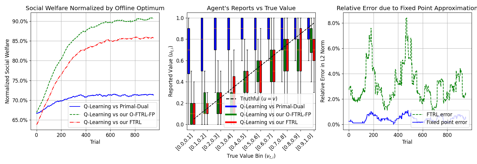
Refer to caption
Figure 3: Vanilla Primal-Dual, Algorithm˜2 with FTRL, and Algorithm˜2 with O-FTRL-FP
Approximation of the Fixed-Point Problem.

Since the minimization in Equation˜11 can be computationally costly to solve, we also give the following alternative approximation of Equation˜10:

𝝀ℓ=argmin𝝀∈𝚲​∑ℓ′<ℓ∑τ∈ℰℓ′(𝝆−𝒄τ,iτ)𝖳​𝝀+𝒈~ℓ​(𝝀)𝖳​𝝀+1ηℓ​Ψ​(𝝀),\bm{\lambda}_{\ell}=\operatornamewithlimits{\mathrm{argmin}}_{\bm{\lambda}\in\bm{\Lambda}}\sum_{\ell^{\prime}<\ell}\sum_{\tau\in\mathcal{E}_{\ell^{\prime}}}(\bm{\rho}-\bm{c}_{\tau,i_{\tau}})^{\mathsf{T}}\bm{\lambda}+\widetilde{\bm{g}}_{\ell}({\color[rgb]{1,0,1}\definecolor[named]{pgfstrokecolor}{rgb}{1,0,1}\pgfsys@color@cmyk@stroke{0}{1}{0}{0}\pgfsys@color@cmyk@fill{0}{1}{0}{0}\bm{\lambda}})^{\mathsf{T}}\bm{\lambda}+\frac{1}{\eta_{\ell}}\Psi(\bm{\lambda}), (12)

where we replace the original 𝒈~ℓ​(𝝀ℓ)\widetilde{\bm{g}}_{\ell}(\bm{\lambda}_{\ell}) with 𝒈~ℓ​(𝝀)\widetilde{\bm{g}}_{\ell}(\bm{\lambda}). The rationale of this approximation is that ∥∇𝒈~ℓ​(𝝀)∥\lVert\nabla\widetilde{\bm{g}}_{\ell}(\bm{\lambda})\rVert is reasonably small: According to Lemma˜C.5, for any 𝝀1,𝝀2∈𝚲\bm{\lambda}_{1},\bm{\lambda}_{2}\in\bm{\Lambda} such that ∥𝝀1−𝝀2∥1≤ϵ\lVert\bm{\lambda}_{1}-\bm{\lambda}_{2}\rVert_{1}\leq\epsilon, 𝒈~ℓ​(𝝀1)≈𝒈~ℓ​(𝝀2)\widetilde{\bm{g}}_{\ell}(\bm{\lambda}_{1})\approx\widetilde{\bm{g}}_{\ell}(\bm{\lambda}_{2}) w.h.p. Therefore, when the numerical optimization of Equation˜12 has small step sizes, all tentative next-iteration of 𝝀ℓ\bm{\lambda}_{\ell} have very similar g~ℓ​(𝝀ℓ)\widetilde{g}_{\ell}(\bm{\lambda}_{\ell})’s. To further justify this approximation through numerical illustrations, we plot in Figure˜3 the relative difference (in terms of ℓ2\ell_{2}-norm) between Equations˜11 and 12. To help understand how large the relative error is, we additionally plotted the relative error between Equation˜11 and the 𝝀ℓ\bm{\lambda}_{\ell} resulted from vanilla FTRL in Equation˜5.

Discussion of Figure˜3.

In Figure˜3 we additionally plotted the FTRL version, i.e., Algorithm˜2 equipped with FTRL updates in Equation˜5. From the left plot, we can see that FTRL (red) gives slightly worse performance than O-FTRL-FP (green) but significantly outperforms the vanilla primal-dual method (blue), agreeing with our theoretical analyses. From the middle plot, Algorithm˜2 – regardless of equipped with FTRL or O-FTRL-FP (green and red) – incentives agents to be truthful; on the other hand, vanilla primal-dual (blue) encourages agents to misreport a lot. From the right plot, which is a new plot in this section, we empirically illustrate that Equation˜12 serves as a valid efficient approximation to the original fixed-point problem in Equation˜11: The relative error between Equations˜11 and 12 is no more than 1%, while that between O-FTRL-FP and FTRL is much larger than 1%.

6 Conclusion and Future Directions

This paper investigates the dynamic allocation of reusable resources to strategic agents under multi-dimensional long-term cost constraints. We show that standard primal-dual methods, though effective in non-strategic settings, are vulnerable to manipulation when agents act strategically. To address this, we introduce a novel incentive-aware mechanism that stabilizes dual updates via an epoch-based structure and leverages randomized exploration rounds to extract truthful signals. Equipped with a computationally efficient FTRL dual update rule, our mechanism guarantees sublinear regret with respect to an offline benchmark, satisfies all cost constraints, and admits a PBE; further leveraging a novel O-FTRL-FP dual update rule, we boost the regret to 𝒪~⁡(T)\operatorname{\widetilde{\operatorname{\mathcal{O}}}}(\sqrt{T}) that is near-optimal even in non-strategic constrained dynamic resource allocation settings. Looking ahead, several promising research directions remain open. For example, while our mechanism uses monetary transfers to ensure incentive compatibility, many real-world applications – such as organ matching, school admissions, or vaccine distribution – operate under non-monetary constraints. Extending our framework to such settings is an important step toward more broadly applicable mechanism design.

References

  • Adan et al. (2009) Ivo Adan, Jos Bekkers, Nico Dellaert, Jan Vissers, and Xiaoting Yu. Patient mix optimisation and stochastic resource requirements: A case study in cardiothoracic surgery planning. Health care management science, 12:129–141, 2009.
  • Agrawal et al. (2014) Shipra Agrawal, Zizhuo Wang, and Yinyu Ye. A dynamic near-optimal algorithm for online linear programming. Operations Research, 62(4):876–890, 2014.
  • Amin et al. (2013) Kareem Amin, Afshin Rostamizadeh, and Umar Syed. Learning prices for repeated auctions with strategic buyers. Advances in neural information processing systems, 26, 2013.
  • Amin et al. (2014) Kareem Amin, Afshin Rostamizadeh, and Umar Syed. Repeated contextual auctions with strategic buyers. Advances in Neural Information Processing Systems, 27, 2014.
  • Arlotto and Gurvich (2019) Alessandro Arlotto and Itai Gurvich. Uniformly bounded regret in the multisecretary problem. Stochastic Systems, 9(3):231–260, 2019.
  • Arrow (1950) Kenneth J Arrow. A difficulty in the concept of social welfare. Journal of political economy, 58(4):328–346, 1950.
  • Badanidiyuru et al. (2018) Ashwinkumar Badanidiyuru, Robert Kleinberg, and Aleksandrs Slivkins. Bandits with knapsacks. Journal of the ACM (JACM), 65(3):1–55, 2018.
  • Balseiro and Gur (2019) Santiago R Balseiro and Yonatan Gur. Learning in repeated auctions with budgets: Regret minimization and equilibrium. Management Science, 65(9):3952–3968, 2019.
  • Balseiro et al. (2019) Santiago R Balseiro, Huseyin Gurkan, and Peng Sun. Multiagent mechanism design without money. Operations Research, 67(5):1417–1436, 2019.
  • Balseiro et al. (2023) Santiago R Balseiro, Haihao Lu, and Vahab Mirrokni. The best of many worlds:: Dual mirror descent for online allocation problems. Operations Research, 71(1):101–119, 2023.
  • Banerjee et al. (2023) Siddhartha Banerjee, Giannis Fikioris, and Eva Tardos. Robust pseudo-markets for reusable public resources. In Proceedings of the 24th ACM Conference on Economics and Computation, pages 241–241, 2023.
  • Berriaud et al. (2024) Damien Berriaud, Ezzat Elokda, Devansh Jalota, Emilio Frazzoli, Marco Pavone, and Florian Dörfler. To spend or to gain: Online learning in repeated karma auctions. arXiv preprint arXiv:2403.04057, 2024.
  • Bertsekas et al. (2003) Dimitri Bertsekas, Angelia Nedic, and Asuman Ozdaglar. Convex analysis and optimization, volume 1. Athena Scientific, 2003.
  • Blanchard and Jaillet (2024) Moise Blanchard and Patrick Jaillet. Near-optimal mechanisms for resource allocation without monetary transfers. arXiv preprint arXiv:2408.10066, 2024.
  • Buyya et al. (2008) Rajkumar Buyya, Chee Shin Yeo, and Srikumar Venugopal. Market-oriented cloud computing: Vision, hype, and reality for delivering it services as computing utilities. In 2008 10th IEEE international conference on high performance computing and communications, pages 5–13. Ieee, 2008.
  • Castiglioni et al. (2022) Matteo Castiglioni, Andrea Celli, and Christian Kroer. Online learning with knapsacks: the best of both worlds. In International Conference on Machine Learning, pages 2767–2783. PMLR, 2022.
  • Cesa-Bianchi et al. (2024a) Nicolò Cesa-Bianchi, Tommaso Cesari, Roberto Colomboni, Federico Fusco, and Stefano Leonardi. Regret analysis of bilateral trade with a smoothed adversary. Journal of Machine Learning Research, 25(234):1–36, 2024a.
  • Cesa-Bianchi et al. (2024b) Nicolò Cesa-Bianchi, Tommaso Cesari, Roberto Colomboni, Federico Fusco, and Stefano Leonardi. The role of transparency in repeated first-price auctions with unknown valuations. In Proceedings of the 56th Annual ACM Symposium on Theory of Computing, pages 225–236, 2024b.
  • Clarke (1971) Edward H Clarke. Multipart pricing of public goods. Public choice, pages 17–33, 1971.
  • Cole et al. (2013) Richard Cole, Vasilis Gkatzelis, and Gagan Goel. Positive results for mechanism design without money. In Proceedings of the 2013 international conference on Autonomous agents and multi-agent systems, pages 1165–1166, 2013.
  • Dai et al. (2025) Yan Dai, Moise Blanchard, and Patrick Jaillet. Non-monetary mechanism design without distributional information: Using scarce audits wisely. arXiv preprint arXiv:2502.08412, 2025.
  • Dekel et al. (2014) Ofer Dekel, Jian Ding, Tomer Koren, and Yuval Peres. Bandits with switching costs: T 2/3 regret. In Proceedings of the forty-sixth annual ACM symposium on Theory of computing, pages 459–467, 2014.
  • Devanur and Hayes (2009) Nikhil R Devanur and Thomas P Hayes. The adwords problem: online keyword matching with budgeted bidders under random permutations. In Proceedings of the 10th ACM conference on Electronic commerce, pages 71–78, 2009.
  • Devanur et al. (2019) Nikhil R Devanur, Kamal Jain, Balasubramanian Sivan, and Christopher A Wilkens. Near optimal online algorithms and fast approximation algorithms for resource allocation problems. Journal of the ACM (JACM), 66(1):1–41, 2019.
  • Duchi et al. (2011) John Duchi, Elad Hazan, and Yoram Singer. Adaptive subgradient methods for online learning and stochastic optimization. Journal of machine learning research, 12(7), 2011.
  • Durvasula et al. (2023) Naveen Durvasula, Nika Haghtalab, and Manolis Zampetakis. Smoothed analysis of online non-parametric auctions. In Proceedings of the 24th ACM Conference on Economics and Computation, pages 540–560, 2023.
  • Feldman et al. (2010) Jon Feldman, Monika Henzinger, Nitish Korula, Vahab S Mirrokni, and Cliff Stein. Online stochastic packing applied to display ad allocation. In European Symposium on Algorithms, pages 182–194. Springer, 2010.
  • Fikioris et al. (2023) Giannis Fikioris, Siddhartha Banerjee, and Éva Tardos. Online resource sharing via dynamic max-min fairness: efficiency, robustness and non-stationarity. arXiv preprint arXiv:2310.08881, 2023.
  • Galgana and Golrezaei (2025) Rigel Galgana and Negin Golrezaei. Learning in repeated multiunit pay-as-bid auctions. Manufacturing & Service Operations Management, 27(1):200–229, 2025.
  • Gibbard (1973) A. Gibbard. Manipulation of voting schemes: A general result. Econometrica, 41(4):587–601, 1973.
  • Golrezaei et al. (2014) Negin Golrezaei, Hamid Nazerzadeh, and Paat Rusmevichientong. Real-time optimization of personalized assortments. Management Science, 60(6):1532–1551, 2014.
  • Golrezaei et al. (2020) Negin Golrezaei, Patrick Jaillet, and Jason Cheuk Nam Liang. No-regret learning in price competitions under consumer reference effects. Advances in Neural Information Processing Systems, 33:21416–21427, 2020.
  • Golrezaei et al. (2021a) Negin Golrezaei, Adel Javanmard, and Vahab Mirrokni. Dynamic incentive-aware learning:: Robust pricing in contextual auctions. Operations Research, 69(1):297–314, 2021a.
  • Golrezaei et al. (2021b) Negin Golrezaei, Max Lin, Vahab Mirrokni, and Hamid Nazerzadeh. Boosted second price auctions: Revenue optimization for heterogeneous bidders. In Proceedings of the 27th ACM SIGKDD Conference on Knowledge Discovery & Data Mining, pages 447–457, 2021b.
  • Golrezaei et al. (2023) Negin Golrezaei, Patrick Jaillet, and Jason Cheuk Nam Liang. Incentive-aware contextual pricing with non-parametric market noise. In International Conference on Artificial Intelligence and Statistics, pages 9331–9361. PMLR, 2023.
  • Gorokh et al. (2021a) Artur Gorokh, Siddhartha Banerjee, and Krishnamurthy Iyer. The remarkable robustness of the repeated fisher market. In Proceedings of the 22nd ACM Conference on Economics and Computation, pages 562–562, 2021a.
  • Gorokh et al. (2021b) Artur Gorokh, Siddhartha Banerjee, and Krishnamurthy Iyer. From monetary to nonmonetary mechanism design via artificial currencies. Mathematics of Operations Research, 46(3):835–855, 2021b.
  • Groves (1973) Theodore Groves. Incentives in teams. Econometrica: Journal of the Econometric Society, pages 617–631, 1973.
  • Guo and Conitzer (2010) Mingyu Guo and Vincent Conitzer. Strategy-proof allocation of multiple items between two agents without payments or priors. In AAMAS, pages 881–888, 2010.
  • Gupta and Molinaro (2016) Anupam Gupta and Marco Molinaro. How the experts algorithm can help solve lps online. Mathematics of Operations Research, 41(4):1404–1431, 2016.
  • Han et al. (2011) Li Han, Chunzhi Su, Linpeng Tang, and Hongyang Zhang. On strategy-proof allocation without payments or priors. In International Workshop on Internet and Network Economics, pages 182–193. Springer, 2011.
  • Jalota et al. (2024) Devansh Jalota, Matthew Tsao, and Marco Pavone. Catch me if you can: Combatting fraud in artificial currency based government benefits programs. arXiv preprint arXiv:2402.16162, 2024.
  • Kanoria and Nazerzadeh (2014) Yash Kanoria and Hamid Nazerzadeh. Dynamic reserve prices for repeated auctions: Learning from bids. In Web and Internet Economics: 10th International Conference, volume 8877, page 232. Springer, 2014.
  • Kesselheim et al. (2018) Thomas Kesselheim, Klaus Radke, Andreas Tonnis, and Berthold Vocking. Primal beats dual on online packing lps in the random-order model. SIAM Journal on Computing, 47(5):1939–1964, 2018.
  • Kohler and Lucchi (2017) Jonas Moritz Kohler and Aurelien Lucchi. Sub-sampled cubic regularization for non-convex optimization. In International Conference on Machine Learning, pages 1895–1904. PMLR, 2017.
  • Koufogiannakis and Young (2014) Christos Koufogiannakis and Neal E Young. A nearly linear-time ptas for explicit fractional packing and covering linear programs. Algorithmica, 70:648–674, 2014.
  • Li et al. (2023) Xiaocheng Li, Chunlin Sun, and Yinyu Ye. Simple and fast algorithm for binary integer and online linear programming. Mathematical Programming, 200(2):831–875, 2023.
  • Miralles (2012) Antonio Miralles. Cardinal bayesian allocation mechanisms without transfers. Journal of Economic Theory, 147(1):179–206, 2012.
  • Molinaro and Ravi (2014) Marco Molinaro and Ramamoorthi Ravi. The geometry of online packing linear programs. Mathematics of Operations Research, 39(1):46–59, 2014.
  • Munkres (2000) J.R. Munkres. Topology. Featured Titles for Topology. Prentice Hall, Incorporated, 2000. ISBN 9780131816299. URL https://books.google.com/books?id=XjoZAQAAIAAJ.
  • Nejad et al. (2014) Mahyar Movahed Nejad, Lena Mashayekhy, and Daniel Grosu. Truthful greedy mechanisms for dynamic virtual machine provisioning and allocation in clouds. IEEE transactions on parallel and distributed systems, 26(2):594–603, 2014.
  • Orabona (2019) Francesco Orabona. A modern introduction to online learning. arXiv preprint arXiv:1912.13213, 2019.
  • Rakhlin and Sridharan (2013) Alexander Rakhlin and Karthik Sridharan. Online learning with predictable sequences. In Conference on Learning Theory, pages 993–1019. PMLR, 2013.
  • Satterthwaite (1975) N.A. Satterthwaite. Strategy-proofness and Arrow’s conditions: Existence and correspondence theorems for voting procedures and social welfare functions. Journal of Economic Theory, 10(2):187–217, 1975.
  • Stummer et al. (2004) Christian Stummer, Karl Doerner, Axel Focke, and Kurt Heidenberger. Determining location and size of medical departments in a hospital network: A multiobjective decision support approach. Health care management science, 7:63–71, 2004.
  • Sun et al. (2020) Rui Sun, Xinshang Wang, and Zijie Zhou. Near-optimal primal-dual algorithms for quantity-based network revenue management. arXiv preprint arXiv:2011.06327, 2020.
  • Vickrey (1961) William Vickrey. Counterspeculation, auctions, and competitive sealed tenders. The Journal of finance, 16(1):8–37, 1961.
  • Watkins and Dayan (1992) Christopher JCH Watkins and Peter Dayan. Q-learning. Machine learning, 8:279–292, 1992.
  • Williams (1991) David Williams. Probability with martingales. Cambridge university press, 1991.
  • Yang et al. (2024) Zongjun Yang, Luofeng Liao, Yuan Gao, and Christian Kroer. Online fair allocation with best-of-many-worlds guarantees. arXiv preprint arXiv:2408.02403, 2024.
  • Yin et al. (2022) Steven Yin, Shipra Agrawal, and Assaf Zeevi. Online allocation and learning in the presence of strategic agents. Advances in Neural Information Processing Systems, 35:6333–6344, 2022.
  • Zimmert and Lattimore (2022) Julian Zimmert and Tor Lattimore. Return of the bias: Almost minimax optimal high probability bounds for adversarial linear bandits. In Conference on Learning Theory, pages 3285–3312. PMLR, 2022.
\appendixpage
\startcontents

[section] \printcontents[section]l1

Appendix A Proof of Main Theorems

A.1 Main Theorem for Algorithm˜2 with FTRL

Theorem A.1 (Formal Version of Theorem˜3.1: Algorithm˜2 with FTRL).

In Algorithm˜2, let

L=T1/3,ℰℓ=[(ℓ−1)​TL+1,ℓ​TL],ηℓ=∥𝝆−1∥22​d​(∑ℓ′=1ℓ|ℰℓ|2)−1/2,Ψ​(𝝀)=12​∥𝝀∥22,L=T^{1/3},\leavevmode\nobreak\ \mathcal{E}_{\ell}=\left[(\ell-1)\frac{T}{L}+1,\ell\frac{T}{L}\right],\leavevmode\nobreak\ \eta_{\ell}=\frac{\lVert\bm{\rho}^{-1}\rVert_{2}}{\sqrt{2d}}\left(\sum_{\ell^{\prime}=1}^{\ell}\lvert\mathcal{E}_{\ell}\rvert^{2}\right)^{-1/2},\leavevmode\nobreak\ \Psi(\bm{\lambda})=\frac{1}{2}\lVert\bm{\lambda}\rVert_{2}^{2},

and the sub-routine 𝒜\mathcal{A} chosen as FTRL (Equation˜5). Then under Assumptions˜1 and 3, there exists a PBE of agents’ joint strategies under Algorithm˜2, denoted by 𝛑∗\bm{\pi}^{\ast}, such that

ℜT​(𝝅∗,Algorithm˜2 with Equation˜5)\displaystyle\quad\mathfrak{R}_{T}(\bm{\pi}^{\ast},\text{\lx@cref{creftypecap~refnum}{alg:mech} with \lx@cref{creftypecap~refnum}{eq:lambda FTRL}})
≤T2/3​(4+4​K2​ϵc​∥𝝆−1∥1+5​log⁡T1/3+log⁡(1+4​(1+∥𝝆−1∥1)​K​T4/3)log⁡γ−1+2​d​∥𝝆−1∥2)+∥𝝆−1∥1,\displaystyle\leq T^{2/3}\left(4+4K^{2}\epsilon_{c}\lVert\bm{\rho}^{-1}\rVert_{1}+5\log T^{1/3}+\frac{\log(1+4(1+\lVert\bm{\rho}^{-1}\rVert_{1})KT^{4/3})}{\log\gamma^{-1}}+\sqrt{2d}\lVert\bm{\rho}^{-1}\rVert_{2}\right)+\lVert\bm{\rho}^{-1}\rVert_{1},
and ​𝔅T​(𝝅∗,Algorithm˜2 with Equation˜5)=0.\displaystyle\text{and }\mathfrak{B}_{T}(\bm{\pi}^{\ast},\text{\lx@cref{creftypecap~refnum}{alg:mech} with \lx@cref{creftypecap~refnum}{eq:lambda FTRL}})=0.

Specifically, when only focusing on polynomial dependencies on d,Kd,K, and TT, we have

ℜT​(𝝅∗,Algorithm˜2 with Equation˜5)\displaystyle\mathfrak{R}_{T}(\bm{\pi}^{\ast},\text{\lx@cref{creftypecap~refnum}{alg:mech} with \lx@cref{creftypecap~refnum}{eq:lambda FTRL}}) =𝒪~d,K,T⁡((K2+d)​T2/3),\displaystyle=\operatorname{\widetilde{\operatorname{\mathcal{O}}}}_{d,K,T}((K^{2}+\sqrt{d})T^{2/3}),
𝔅T​(𝝅∗,Algorithm˜2 with Equation˜5)\displaystyle\mathfrak{B}_{T}(\bm{\pi}^{\ast},\text{\lx@cref{creftypecap~refnum}{alg:mech} with \lx@cref{creftypecap~refnum}{eq:lambda FTRL}}) =0.\displaystyle=0.
Proof.

As mentioned in the main text, we introduce an intermediate allocation:

i~t∗:=argmaxi∈{0}∪[K](vt,i−𝝀ℓ𝖳​𝒄t,i),∀ℓ∈[L],t∈ℰℓ.\widetilde{i}_{t}^{\ast}:=\operatornamewithlimits{\mathrm{argmax}}_{i\in\{0\}\cup[K]}\left(v_{t,i}-\bm{\lambda}_{\ell}^{\mathsf{T}}\bm{c}_{t,i}\right),\quad\forall\ell\in[L],t\in\mathcal{E}_{\ell}. (13)

Define stopping time 𝒯v\mathcal{T}_{v} as the last round where no constraint violations can happen:

𝒯v:=min{t∈[T]|∑τ=1t𝒄τ,iτ+𝟏≰T𝝆}∪{T+1}.\mathcal{T}_{v}:=\min\left\{t\in[T]\mathrel{}\middle|\mathrel{}\sum_{{\tau}=1}^{t}\bm{c}_{{\tau},i_{\tau}}+\bm{1}\not\leq T\bm{\rho}\right\}\cup\{T+1\}. (14)

Thus in rounds t≤𝒯vt\leq\mathcal{T}_{v}, Line˜10 never rejects our allocation iti_{t}. Decompose the regret ℜT\mathfrak{R}_{T} as

ℜT\displaystyle\mathfrak{R}_{T} =𝔼​[∑t=1T(vt,it∗−vt,it)]≤𝔼[∑t=1𝒯v(vt,i~t∗−vt,it)⏟PrimalAlloc+∑t=1𝒯v(vt,it∗−vt,i~t∗)⏟DualVar+(T−𝒯v)⏟NoAct].\displaystyle=\mathbb{E}\left[\sum_{t=1}^{T}(v_{t,i_{t}^{\ast}}-v_{t,i_{t}})\right]\leq\operatornamewithlimits{\mathbb{E}}\Bigg{[}\underbrace{\sum_{t=1}^{\mathcal{T}_{v}}(v_{t,\widetilde{i}_{t}^{\ast}}-v_{t,i_{t}})}_{\textsc{PrimalAlloc}}+\underbrace{\sum_{t=1}^{\mathcal{T}_{v}}(v_{t,i_{t}^{\ast}}-v_{t,\widetilde{i}_{t}^{\ast}})}_{\textsc{DualVar}}+\underbrace{\vphantom{\sum_{t=1}^{\mathcal{T}_{v}}}(T-\mathcal{T}_{v})}_{\textsc{NoAct}}\Bigg{]}.

From Theorem˜B.5 presented later in Appendix˜B, there exists a PBE 𝝅∗\bm{\pi}^{\ast} such that

𝔼[PrimalAlloc]≤∑ℓ=1L(Nℓ+3),\displaystyle\operatornamewithlimits{\mathbb{E}}[\textsc{PrimalAlloc}]\leq\sum_{\ell=1}^{L}(N_{\ell}+3),\quad
Nℓ=1+4​K2​ϵc​∥𝝆−1∥1+5​log⁡|ℰℓ|+logγ−1⁡(1+4​(1+∥𝝆−1∥1)​K​|ℰℓ|4).\displaystyle N_{\ell}=1+4K^{2}\epsilon_{c}\lVert\bm{\rho}^{-1}\rVert_{1}+5\log\lvert\mathcal{E}_{\ell}\rvert+\log_{\gamma^{-1}}(1+4(1+\lVert\bm{\rho}^{-1}\rVert_{1})K\lvert\mathcal{E}_{\ell}\rvert^{4}).

This is the first main technical contribution of our paper, namely justifying that Algorithm˜2 – equipped with epoch-based lazy updates, uniform exploration rounds, and dual-adjusted allocation and payment plans – is robust to agents’ strategic manipulations.

From Theorem˜C.2 presented later in Appendix˜C, when setting

Ψ​(𝝀)=12​∥𝝀∥22,ηℓ=∥𝝆−1∥22​d​(∑ℓ′=1ℓ|ℰℓ|2)−1/2,\Psi(\bm{\lambda})=\frac{1}{2}\lVert\bm{\lambda}\rVert_{2}^{2},\quad\eta_{\ell}=\frac{\lVert\bm{\rho}^{-1}\rVert_{2}}{\sqrt{2d}}\left(\sum_{\ell^{\prime}=1}^{\ell}\lvert\mathcal{E}_{\ell}\rvert^{2}\right)^{-1/2},

and under the same 𝝅∗\bm{\pi}^{\ast}, the 𝔼[DualVar]\operatornamewithlimits{\mathbb{E}}[\textsc{DualVar}] term is bounded by

𝔼[DualVar]≤2​d​∥𝝆−1∥2⋅∑ℓ=1L|ℰℓ|2+∑ℓ=1L(Nℓ+3)​∥𝝆−1∥1+∥𝝆−1∥1.\operatornamewithlimits{\mathbb{E}}[\textsc{DualVar}]\leq\sqrt{2d}\lVert\bm{\rho}^{-1}\rVert_{2}\cdot\sqrt{\sum_{\ell=1}^{L}\lvert\mathcal{E}_{\ell}\rvert^{2}}+\sum_{\ell=1}^{L}(N_{\ell}+3)\lVert\bm{\rho}^{-1}\rVert_{1}+\lVert\bm{\rho}^{-1}\rVert_{1}.

Thus it only remains to balance the ∑ℓ=1LNℓ=𝒪~⁡(L)\sum_{\ell=1}^{L}N_{\ell}=\operatorname{\widetilde{\operatorname{\mathcal{O}}}}(L) term and ∑ℓ=1L|ℰℓ|2\sqrt{\sum_{\ell=1}^{L}\lvert\mathcal{E}_{\ell}\rvert^{2}} term. Setting L=T2/3L=T^{2/3} and |ℰℓ|=T1/3\lvert\mathcal{E}_{\ell}\rvert=T^{1/3} for all ℓ∈[L]\ell\in[L] ensures ∑ℓ=1L|ℰℓ|2=T2/3×T2/3=T2/3\sqrt{\sum_{\ell=1}^{L}\lvert\mathcal{E}_{\ell}\rvert^{2}}=\sqrt{T^{2/3}\times T^{2/3}}=T^{2/3} and thus

ℜT​(𝝅∗,Algorithm˜2 with Equation˜5)≤𝔼[PrimalAlloc]+𝔼[DualVar]\displaystyle\quad\mathfrak{R}_{T}(\bm{\pi}^{\ast},\text{\lx@cref{creftypecap~refnum}{alg:mech} with \lx@cref{creftypecap~refnum}{eq:lambda FTRL}})\leq\operatornamewithlimits{\mathbb{E}}[\textsc{PrimalAlloc}]+\operatornamewithlimits{\mathbb{E}}[\textsc{DualVar}]
≤∑ℓ=1L(Nℓ+3)+2​d​∥𝝆−1∥2⋅T2/3+∑ℓ=1L(Nℓ+3)​∥𝝆−1∥1+∥𝝆−1∥1\displaystyle\leq\sum_{\ell=1}^{L}(N_{\ell}+3)+\sqrt{2d}\lVert\bm{\rho}^{-1}\rVert_{2}\cdot T^{2/3}+\sum_{\ell=1}^{L}(N_{\ell}+3)\lVert\bm{\rho}^{-1}\rVert_{1}+\lVert\bm{\rho}^{-1}\rVert_{1}
=∑ℓ=1L(Nℓ+3)​(1+∥𝝆−1∥1)+2​d​∥𝝆−1∥2⋅T2/3+∥𝝆−1∥1.\displaystyle=\sum_{\ell=1}^{L}(N_{\ell}+3)(1+\lVert\bm{\rho}^{-1}\rVert_{1})+\sqrt{2d}\lVert\bm{\rho}^{-1}\rVert_{2}\cdot T^{2/3}+\lVert\bm{\rho}^{-1}\rVert_{1}.

Plugging our specific epoching rule that L=T2/3L=T^{2/3} and |ℰℓ|=T1/3\lvert\mathcal{E}_{\ell}\rvert=T^{1/3} into NℓN_{\ell}, we get

∑ℓ=1L(Nℓ+3)≤T2/3×(4+4​K2​ϵc​∥𝝆−1∥1+5​log⁡T1/3+log⁡(1+4​(1+∥𝝆−1∥1)​K​T4/3)log⁡γ−1),\sum_{\ell=1}^{L}(N_{\ell}+3)\leq T^{2/3}\times\left(4+4K^{2}\epsilon_{c}\lVert\bm{\rho}^{-1}\rVert_{1}+5\log T^{1/3}+\frac{\log(1+4(1+\lVert\bm{\rho}^{-1}\rVert_{1})KT^{4/3})}{\log\gamma^{-1}}\right),

which gives our claimed bound after rearrangement. For 𝔅T\mathfrak{B}_{T}, since Line˜10 rejects every infeasible allocation, we trivially have 𝔅T​(𝝅∗,Algorithm˜2 with Equation˜5)=0\mathfrak{B}_{T}(\bm{\pi}^{\ast},\text{\lx@cref{creftypecap~refnum}{alg:mech} with \lx@cref{creftypecap~refnum}{eq:lambda FTRL}})=0. ∎

A.2 Main Theorem for Algorithm˜2 with O-FTRL-FP

Theorem A.2 (Formal Version of Theorem˜3.2: Algorithm˜2 with O-FTRL-FP).

In Algorithm˜2, let

L=⌈log⁡T⌉,ℰℓ=[2ℓ−1,min⁡(2ℓ−1,T)],ηℓ=∥𝝆−1∥2112​d​K2​(∑ℓ′=1ℓ|ℰℓ|)−1/2,Ψ​(𝝀)=12​∥𝝀∥22,L=\lceil\log T\rceil,\leavevmode\nobreak\ \mathcal{E}_{\ell}=\left[2^{\ell-1},\min(2^{\ell}-1,T)\right],\leavevmode\nobreak\ \eta_{\ell}=\frac{\lVert\bm{\rho}^{-1}\rVert_{2}}{\sqrt{112d}K^{2}}\left(\sum_{\ell^{\prime}=1}^{\ell}\lvert\mathcal{E}_{\ell}\rvert\right)^{-1/2},\leavevmode\nobreak\ \Psi(\bm{\lambda})=\frac{1}{2}\lVert\bm{\lambda}\rVert_{2}^{2},

and the sub-routine 𝒜\mathcal{A} chosen as O-FTRL-FP (Equation˜6). Then under Assumptions˜1 and 3, there exists a PBE of agents’ joint strategies under Algorithm˜2, denoted by 𝛑∗\bm{\pi}^{\ast}, such that

ℜT​(𝝅∗,Algorithm˜2 with Equation˜6)\displaystyle\quad\mathfrak{R}_{T}(\bm{\pi}^{\ast},\text{\lx@cref{creftypecap~refnum}{alg:mech} with \lx@cref{creftypecap~refnum}{eq:lambda O-FTRL-FP}})
≤2​T​(∥𝝆−1∥222+8​d2+48​d​log⁡(d​T​L)+48​d​∑j=1dlog⁡d​K2​ϵc​TT​ρj+16​d+10)\displaystyle\leq 2\sqrt{T}\left(\frac{\lVert\bm{\rho}^{-1}\rVert_{2}^{2}}{2}+8d^{2}+48d\log(dTL)+48d\sum_{j=1}^{d}\log\frac{dK^{2}\epsilon_{c}T}{T\rho_{j}}+16d+10\right)
+∑ℓ=1L(2​Nℓ2+(Nℓ+3)​(∥𝝆−1∥1+1)+8​d​Mℓ2)+3​∥𝝆−1∥1,\displaystyle\quad+\sum_{\ell=1}^{L}\left(2N_{\ell}^{2}+(N_{\ell}+3)(\lVert\bm{\rho}^{-1}\rVert_{1}+1)+8dM_{\ell}^{2}\right)+3\lVert\bm{\rho}^{-1}\rVert_{1},
and ​𝔅T​(𝝅∗,Algorithm˜2 with Equation˜6)=0,\displaystyle\text{and }\mathfrak{B}_{T}(\bm{\pi}^{\ast},\text{\lx@cref{creftypecap~refnum}{alg:mech} with \lx@cref{creftypecap~refnum}{eq:lambda O-FTRL-FP}})=0,

where NℓN_{\ell} and MℓM_{\ell} is defined as follows for all ℓ∈[L]\ell\in[L].

Nℓ\displaystyle N_{\ell} =1+4​K2​ϵc​∥𝝆−1∥1+5​log⁡|ℰℓ|+logγ−1⁡(1+4​(1+∥𝝆−1∥1)​K​|ℰℓ|4),\displaystyle=1+4K^{2}\epsilon_{c}\lVert\bm{\rho}^{-1}\rVert_{1}+5\log\lvert\mathcal{E}_{\ell}\rvert+\log_{\gamma^{-1}}(1+4(1+\lVert\bm{\rho}^{-1}\rVert_{1})K\lvert\mathcal{E}_{\ell}\rvert^{4}),
Mℓ\displaystyle M_{\ell} =ℓ​logγ−1⁡(1+4​(1+∥𝝆−1∥1)​K​|ℰℓ|3⋅4​ℓ​δ−1)+4​ℓ​ϵc​∥𝝆−1∥1+4​(log⁡(d​T)+∑j=1dlog⁡d​K2​ϵc​Tρj​ϵ).\displaystyle=\ell\log_{\gamma^{-1}}\left(1+4(1+\lVert\bm{\rho}^{-1}\rVert_{1})K\lvert\mathcal{E}_{\ell}\rvert^{3}\cdot 4\ell\delta^{-1}\right)+4\ell\epsilon_{c}\lVert\bm{\rho}^{-1}\rVert_{1}+4\left(\log(dT)+\sum_{j=1}^{d}\log\frac{dK^{2}\epsilon_{c}T}{\rho_{j}\epsilon}\right).

Specifically, when only focusing on polynomial dependencies on d,Kd,K, and TT, we have

ℜT​(𝝅∗,Algorithm˜2 with Equation˜6)\displaystyle\mathfrak{R}_{T}(\bm{\pi}^{\ast},\text{\lx@cref{creftypecap~refnum}{alg:mech} with \lx@cref{creftypecap~refnum}{eq:lambda O-FTRL-FP}}) =𝒪~d,K,T⁡(d2​T+K4),\displaystyle=\operatorname{\widetilde{\operatorname{\mathcal{O}}}}_{d,K,T}(d^{2}\sqrt{T}+K^{4}),
𝔅T​(𝝅∗,Algorithm˜2 with Equation˜6)\displaystyle\mathfrak{B}_{T}(\bm{\pi}^{\ast},\text{\lx@cref{creftypecap~refnum}{alg:mech} with \lx@cref{creftypecap~refnum}{eq:lambda O-FTRL-FP}}) =0.\displaystyle=0.
Proof.

The proof follows the same structure as the previous one, but the treatment of the 𝔼[DualVar]\operatornamewithlimits{\mathbb{E}}[\textsc{DualVar}] term is extremely challenging and requests delicate analytical tools; we refer the readers to Theorem˜C.3 for more details. We still include a full proof of this theorem for completeness.

As mentioned in the main text, we introduce an intermediate allocation:

i~t∗:=argmaxi∈{0}∪[K](vt,i−𝝀ℓ𝖳​𝒄t,i),∀ℓ∈[L],t∈ℰℓ.\widetilde{i}_{t}^{\ast}:=\operatornamewithlimits{\mathrm{argmax}}_{i\in\{0\}\cup[K]}\left(v_{t,i}-\bm{\lambda}_{\ell}^{\mathsf{T}}\bm{c}_{t,i}\right),\quad\forall\ell\in[L],t\in\mathcal{E}_{\ell}.

Define stopping time 𝒯v\mathcal{T}_{v} as the last round where no constraint violations can happen:

𝒯v:=min{t∈[T]|∑τ=1t𝒄τ,iτ+𝟏≰T𝝆}∪{T+1}.\mathcal{T}_{v}:=\min\left\{t\in[T]\mathrel{}\middle|\mathrel{}\sum_{{\tau}=1}^{t}\bm{c}_{{\tau},i_{\tau}}+\bm{1}\not\leq T\bm{\rho}\right\}\cup\{T+1\}.

Thus in rounds t≤𝒯vt\leq\mathcal{T}_{v}, Line˜10 never rejects our allocation iti_{t}. Decompose the regret ℜT\mathfrak{R}_{T} as

ℜT\displaystyle\mathfrak{R}_{T} =𝔼​[∑t=1T(vt,it∗−vt,it)]≤𝔼[∑t=1𝒯v(vt,i~t∗−vt,it)⏟PrimalAlloc+∑t=1𝒯v(vt,it∗−vt,i~t∗)⏟DualVar+(T−𝒯v)⏟NoAct].\displaystyle=\mathbb{E}\left[\sum_{t=1}^{T}(v_{t,i_{t}^{\ast}}-v_{t,i_{t}})\right]\leq\operatornamewithlimits{\mathbb{E}}\Bigg{[}\underbrace{\sum_{t=1}^{\mathcal{T}_{v}}(v_{t,\widetilde{i}_{t}^{\ast}}-v_{t,i_{t}})}_{\textsc{PrimalAlloc}}+\underbrace{\sum_{t=1}^{\mathcal{T}_{v}}(v_{t,i_{t}^{\ast}}-v_{t,\widetilde{i}_{t}^{\ast}})}_{\textsc{DualVar}}+\underbrace{\vphantom{\sum_{t=1}^{\mathcal{T}_{v}}}(T-\mathcal{T}_{v})}_{\textsc{NoAct}}\Bigg{]}.

For the PrimalAlloc term, we still use Theorem˜B.5 presented later in Appendix˜B (which holds regardless to the dual update rules). Theorem˜B.5 asserts that there exists a PBE 𝝅∗\bm{\pi}^{\ast} such that

𝔼[PrimalAlloc]≤∑ℓ=1L(Nℓ+3),\operatornamewithlimits{\mathbb{E}}[\textsc{PrimalAlloc}]\leq\sum_{\ell=1}^{L}(N_{\ell}+3)\,,

where

Nℓ=1+4​K2​ϵc​∥𝝆−1∥1+5​log⁡|ℰℓ|+logγ−1⁡(1+4​(1+∥𝝆−1∥1)​K​|ℰℓ|4).N_{\ell}=1+4K^{2}\epsilon_{c}\lVert\bm{\rho}^{-1}\rVert_{1}+5\log\lvert\mathcal{E}_{\ell}\rvert+\log_{\gamma^{-1}}(1+4(1+\lVert\bm{\rho}^{-1}\rVert_{1})K\lvert\mathcal{E}_{\ell}\rvert^{4}).

For the DualVar term, as sketched in Sections˜4.2.4 and 4.2.5, the analysis is much more involved than the FTRL counterpart. Via careful investigation, Theorem˜C.3 in Appendix˜C proves that when configuring

Ψ​(𝝀)=12​∥𝝀∥22,L=log⁡T,ℰℓ=[2ℓ−1,min⁡(2ℓ−1,T)],ηℓ=(∑ℓ′=1ℓ|ℰℓ′|)−1/2,\Psi(\bm{\lambda})=\frac{1}{2}\lVert\bm{\lambda}\rVert_{2}^{2},\leavevmode\nobreak\ L=\log T,\leavevmode\nobreak\ \mathcal{E}_{\ell}=[2^{\ell-1},\min(2^{\ell}-1,T)],\leavevmode\nobreak\ \eta_{\ell}=\left(\sum_{\ell^{\prime}=1}^{\ell}\lvert\mathcal{E}_{\ell^{\prime}}\rvert\right)^{-1/2},

we can control the 𝔼[DualVar]\operatornamewithlimits{\mathbb{E}}[\textsc{DualVar}] as

𝔼[DualVar]\displaystyle\operatornamewithlimits{\mathbb{E}}[\textsc{DualVar}] ≤2​T​(∥𝝆−1∥222+8​d2+48​d​log⁡(d​T​L)+48​d​∑j=1dlog⁡d​K2​ϵc​TT​ρj+16​d+10)\displaystyle\leq 2\sqrt{T}\left(\frac{\lVert\bm{\rho}^{-1}\rVert_{2}^{2}}{2}+8d^{2}+48d\log(dTL)+48d\sum_{j=1}^{d}\log\frac{dK^{2}\epsilon_{c}T}{T\rho_{j}}+16d+10\right)
+∑ℓ=1L(2​Nℓ2+(Nℓ+3)​∥𝝆−1∥1+8​d​Mℓ2)+3​∥𝝆−1∥1.\displaystyle\quad+\sum_{\ell=1}^{L}\left(2N_{\ell}^{2}+(N_{\ell}+3)\lVert\bm{\rho}^{-1}\rVert_{1}+8dM_{\ell}^{2}\right)+3\lVert\bm{\rho}^{-1}\rVert_{1}.

where (the definition of NℓN_{\ell} is the same as that in PrimalAlloc)

Nℓ\displaystyle N_{\ell} =1+4​K2​ϵc​∥𝝆−1∥1+5​log⁡|ℰℓ|+logγ−1⁡(1+4​(1+∥𝝆−1∥1)​K​|ℰℓ|4),\displaystyle=1+4K^{2}\epsilon_{c}\lVert\bm{\rho}^{-1}\rVert_{1}+5\log\lvert\mathcal{E}_{\ell}\rvert+\log_{\gamma^{-1}}(1+4(1+\lVert\bm{\rho}^{-1}\rVert_{1})K\lvert\mathcal{E}_{\ell}\rvert^{4}),
Mℓ\displaystyle M_{\ell} =ℓ​logγ−1⁡(1+4​(1+∥𝝆−1∥1)​K​|ℰℓ|3⋅4​ℓ​δ−1)+4​ℓ​ϵc​∥𝝆−1∥1+4​(log⁡(d​T)+∑j=1dlog⁡d​K2​ϵc​Tρj​ϵ).\displaystyle=\ell\log_{\gamma^{-1}}\left(1+4(1+\lVert\bm{\rho}^{-1}\rVert_{1})K\lvert\mathcal{E}_{\ell}\rvert^{3}\cdot 4\ell\delta^{-1}\right)+4\ell\epsilon_{c}\lVert\bm{\rho}^{-1}\rVert_{1}+4\left(\log(dT)+\sum_{j=1}^{d}\log\frac{dK^{2}\epsilon_{c}T}{\rho_{j}\epsilon}\right).

Putting two parts together, we get

ℜT​(𝝅∗,Algorithm˜2 with Equation˜6)≤𝔼[PrimalAlloc]+𝔼[DualVar]\displaystyle\quad\mathfrak{R}_{T}(\bm{\pi}^{\ast},\text{\lx@cref{creftypecap~refnum}{alg:mech} with \lx@cref{creftypecap~refnum}{eq:lambda O-FTRL-FP}})\leq\operatornamewithlimits{\mathbb{E}}[\textsc{PrimalAlloc}]+\operatornamewithlimits{\mathbb{E}}[\textsc{DualVar}]
≤2​T​(∥𝝆−1∥222+8​d2+48​d​log⁡(d​T​L)+48​d​∑j=1dlog⁡d​K2​ϵc​TT​ρj+16​d+10)\displaystyle\leq 2\sqrt{T}\left(\frac{\lVert\bm{\rho}^{-1}\rVert_{2}^{2}}{2}+8d^{2}+48d\log(dTL)+48d\sum_{j=1}^{d}\log\frac{dK^{2}\epsilon_{c}T}{T\rho_{j}}+16d+10\right)
+∑ℓ=1L(2​Nℓ2+(Nℓ+3)​(∥𝝆−1∥1+1)+8​d​Mℓ2)+3​∥𝝆−1∥1.\displaystyle\quad+\sum_{\ell=1}^{L}\left(2N_{\ell}^{2}+(N_{\ell}+3)(\lVert\bm{\rho}^{-1}\rVert_{1}+1)+8dM_{\ell}^{2}\right)+3\lVert\bm{\rho}^{-1}\rVert_{1}.

The bound that 𝔅T​(𝝅∗,Algorithm˜2 with Equation˜6)=0\mathfrak{B}_{T}(\bm{\pi}^{\ast},\text{\lx@cref{creftypecap~refnum}{alg:mech} with \lx@cref{creftypecap~refnum}{eq:lambda O-FTRL-FP}})=0 directly follows from Line˜10 of Algorithm˜2.

For the 𝒪~d,K,T\operatorname{\widetilde{\operatorname{\mathcal{O}}}}_{d,K,T} version, since L≤⌈log2⁡T⌉=𝒪~d,K,T⁡(1)L\leq\lceil\log_{2}T\rceil=\operatorname{\widetilde{\operatorname{\mathcal{O}}}}_{d,K,T}(1) and |ℰℓ|≤T\lvert\mathcal{E}_{\ell}\rvert\leq T for all ℓ\ell, we know Nℓ=𝒪~d,K,T⁡(K2)N_{\ell}=\operatorname{\widetilde{\operatorname{\mathcal{O}}}}_{d,K,T}(K^{2}) and Mℓ=𝒪~d,K,T⁡(ℓ)=𝒪~d,K,T⁡(1)M_{\ell}=\operatorname{\widetilde{\operatorname{\mathcal{O}}}}_{d,K,T}(\ell)=\operatorname{\widetilde{\operatorname{\mathcal{O}}}}_{d,K,T}(1). This gives ℜT=𝒪~d,K,T⁡(d2​T+K4)\mathfrak{R}_{T}=\operatorname{\widetilde{\operatorname{\mathcal{O}}}}_{d,K,T}(d^{2}\sqrt{T}+K^{4}). ∎

Appendix B PrimalAlloc: Regret due to Agents’ Strategic Reports

B.1 IntraEpoch: Agents Lie to Affect Current-Epoch Allocations

Lemma B.1 (Truthfulness of a Cost-Adjusted Second-Price Auction).

Consider a one-shot monetary allocation setting with KK agents. Each agent i∈[K]i\in[K] privately observes their value vi∼𝒱iv_{i}\sim\mathcal{V}_{i} and publicly incurs a known cost ci∼𝒞ic_{i}\sim\mathcal{C}_{i}. Agents submit scalar reports ui∈[0,1]u_{i}\in[0,1], and the planner allocates the item to one agent it∈[K]i_{t}\in[K] and charges payment pitp_{i_{t}}. The utility of the selected agent is vit−pitv_{i_{t}}-p_{i_{t}}, while all others receive zero utility.

Suppose the planner implements the following mechanism:

it=argmaxi∈{0}∪[K](ui−ci),pit=cit+maxj≠it⁡(uj−cj).i_{t}=\operatornamewithlimits{\mathrm{argmax}}_{i\in\{0\}\cup[K]}(u_{i}-c_{i}),\quad p_{i_{t}}=c_{i_{t}}+\max_{j\neq i_{t}}(u_{j}-c_{j}).

Then:

  1. (i)

    For any agent i∈[K]i\in[K] aiming to maximize their expected utility (vi−pi)⋅𝟙​[it=i](v_{i}-p_{i})\cdot\mathbbm{1}[i_{t}=i], truthful reporting ui=viu_{i}=v_{i} is a weakly dominant strategy.

  2. (ii)

    When all agents report truthfully (ui=viu_{i}=v_{i}), the allocation it=argmaxi∈[K](vi−ci)i_{t}=\operatornamewithlimits{\mathrm{argmax}}_{i\in[K]}(v_{i}-c_{i}), i.e., it maximizes the value-minus-cost vi−civ_{i}-c_{i} across all the agents.

Proof.

Define each agent’s pseudo-report as u~i:=ui−ci\widetilde{u}_{i}:=u_{i}-c_{i}, and let u~i∗:=vi−ci\widetilde{u}_{i}^{\ast}:=v_{i}-c_{i} be the truthful pseudo-report. Fix any agent i∈[K]i\in[K] and suppose all other agents’ reports {uj}j≠i\{u_{j}\}_{j\neq i} are fixed. We evaluate the utility 𝒰i\mathcal{U}_{i} that agent ii obtains under various reporting strategies.

Case 1: Truthfully report ui=viu_{i}=v_{i} so that u~i=u~i∗\widetilde{u}_{i}=\widetilde{u}_{i}^{\ast}:

  • •

    If u~i∗>maxj≠i⁡u~j\widetilde{u}_{i}^{\ast}>\max_{j\neq i}\widetilde{u}_{j}, then it=ii_{t}=i, and 𝒰i=vi−ci−maxj≠i⁡u~j=u~i∗−maxj≠i⁡u~j\mathcal{U}_{i}=v_{i}-c_{i}-\max_{j\neq i}\widetilde{u}_{j}=\widetilde{u}_{i}^{\ast}-\max_{j\neq i}\widetilde{u}_{j}.

  • •

    If u~i∗<maxj≠i⁡u~j\widetilde{u}_{i}^{\ast}<\max_{j\neq i}\widetilde{u}_{j}, then it≠ii_{t}\neq i, and 𝒰i=0\mathcal{U}_{i}=0.

Case 2: Over-reporting ui>viu_{i}>v_{i} so u~i>u~i∗\widetilde{u}_{i}>\widetilde{u}_{i}^{\ast}:

  • •

    If u~i>u~i∗>maxj≠i⁡u~j\widetilde{u}_{i}>\widetilde{u}_{i}^{\ast}>\max_{j\neq i}\widetilde{u}_{j}, 𝒰i=u~i∗−maxj≠i⁡u~j\mathcal{U}_{i}=\widetilde{u}_{i}^{\ast}-\max_{j\neq i}\widetilde{u}_{j} (same as truthful).

  • •

    If maxj≠i⁡u~j>u~i>u~i∗\max_{j\neq i}\widetilde{u}_{j}>\widetilde{u}_{i}>\widetilde{u}_{i}^{\ast}, 𝒰i=0\mathcal{U}_{i}=0 (same as truthful).

  • •

    Otherwise if u~i>maxj≠i⁡u~j>u~i∗\widetilde{u}_{i}>\max_{j\neq i}\widetilde{u}_{j}>\widetilde{u}_{i}^{\ast}, 𝒰i=u~i∗−maxj≠i⁡u~j<0\mathcal{U}_{i}=\widetilde{u}_{i}^{\ast}-\max_{j\neq i}\widetilde{u}_{j}<0 (worse than truthful).

Case 3: Under-reporting ui<viu_{i}<v_{i} so u~i<u~i∗\widetilde{u}_{i}<\widetilde{u}_{i}^{\ast}:

  • •

    If u~i∗>u~i>maxj≠i⁡u~j\widetilde{u}_{i}^{\ast}>\widetilde{u}_{i}>\max_{j\neq i}\widetilde{u}_{j}, 𝒰i=u~i∗−maxj≠i⁡u~j\mathcal{U}_{i}=\widetilde{u}_{i}^{\ast}-\max_{j\neq i}\widetilde{u}_{j} (same as truthful).

  • •

    If maxj≠i⁡u~j>u~i∗>u~i\max_{j\neq i}\widetilde{u}_{j}>\widetilde{u}_{i}^{\ast}>\widetilde{u}_{i}, 𝒰i=0\mathcal{U}_{i}=0 (same as truthful).

  • •

    Otherwise, if u~i∗>maxj≠i⁡u~j>u~i\widetilde{u}_{i}^{\ast}>\max_{j\neq i}\widetilde{u}_{j}>\widetilde{u}_{i}, 𝒰i=0\mathcal{U}_{i}=0. But they originally get u~i∗−maxj≠i⁡u~j≥0\widetilde{u}_{i}^{\ast}-\max_{j\neq i}\widetilde{u}_{j}\geq 0.

In all cases, deviating from truth-telling does not improve agent ii’s utility, and may strictly reduce it. Hence, truthful reporting is a weakly dominant strategy, proving claim (i).

For claim (ii), when all agents report truthfully (ui=viu_{i}=v_{i}), the planner allocates the resource to it=arg⁡maxi⁡(vi−ci)i_{t}=\arg\max_{i}(v_{i}-c_{i}), which maximizes net social value. ∎

Theorem B.2 (Intra-Epoch Truthfulness; Formal Theorem˜4.1).

Fix any epoch ℰℓ⊆[T]\mathcal{E}_{\ell}\subseteq[T] and dual variable 𝛌ℓ∈𝚲\bm{\lambda}_{\ell}\in\bm{\Lambda}. Suppose that all the agents, when crafting their reports only consider their discounted gains within the current epoch (Model 2 in Equation˜8), namely Equation˜15. To highlight the different reports, allocations, and payments due to the different agent model, we add a superscript hh.

max{ut,ih}t∈ℰℓ⁡𝔼​[∑t∈ℰℓγt​(vt,i−pt,ih)⋅𝟙​[ith=i]],∀i∈[K].\max_{\{u_{t,i}^{h}\}_{t\in\mathcal{E}_{\ell}}}\leavevmode\nobreak\ \mathbb{E}\left[\sum_{t\in\mathcal{E}_{\ell}}\gamma^{t}(v_{t,i}-p_{t,i}^{h})\cdot\mathbbm{1}[i_{t}^{h}=i]\right],\quad\forall i\in[K]. (15)

The planner, on the other hand, uses the allocation and payment rule in Line˜9. Formally, in round t∈ℰℓt\in\mathcal{E}_{\ell} the planner allocates to the agent with maximal dual-adjusted report – which we denote by ithi_{t}^{h} to highlight its difference with iti_{t} due to the different agent model – and sets payments accordingly:

ith=argmaxi∈{0}∪[K](ut,ih−𝝀ℓ𝖳​𝒄t,i),pt,ithh=𝝀ℓ𝖳​𝒄t,ith+maxj≠ith⁡(ut,jh−𝝀ℓ𝖳​𝒄t,j),∀t∈ℰℓ.i_{t}^{h}=\operatornamewithlimits{\mathrm{argmax}}_{i\in\{0\}\cup[K]}(u_{t,i}^{h}-\bm{\lambda}_{\ell}^{\mathsf{T}}\bm{c}_{t,i}),\quad p_{t,i_{t}^{h}}^{h}=\bm{\lambda}_{\ell}^{\mathsf{T}}\bm{c}_{t,i_{t}^{h}}+\max_{j\neq i_{t}^{h}}(u_{t,j}^{h}-\bm{\lambda}_{\ell}^{\mathsf{T}}\bm{c}_{t,j}),\quad\forall t\in\mathcal{E}_{\ell}.

Then, truthful reporting ut,i=vt,iu_{t,i}=v_{t,i} for all t∈ℰℓt\in\mathcal{E}_{\ell} and all i∈[K]i\in[K] – a joint strategy denoted as Truth\operatorname{\textsc{Truth}} – constitutes a Perfect Bayesian Equilibrium (PBE). Furthermore, under this PBE, the planner always chooses the optimal agent according to dual-adjusted value:

ith=i~t∗:=arg⁡maxi∈[K]⁡(vt,i−𝝀ℓ⊤​𝒄t,i),i_{t}^{h}=\widetilde{i}_{t}^{\ast}:=\arg\max_{i\in[K]}\left(v_{t,i}-\bm{\lambda}_{\ell}^{\top}\bm{c}_{t,i}\right),

and the regret due to intra-epoch misallocations is zero, i.e., 𝔼​[IntraEpoch]=0\mathbb{E}[\textsc{IntraEpoch}]=0.

Proof.

For any round t∈ℰℓt\in\mathcal{E}_{\ell}, we observe that the planner’s allocation and payment plan (ith,𝒑th)(i_{t}^{h},\bm{p}_{t}^{h}) depends only on the current reports 𝒖th\bm{u}_{t}^{h}, current costs 𝒄t\bm{c}_{t}, and the fixed dual variable 𝝀ℓ\bm{\lambda}_{\ell}. Specifically, it does not depend on historical reports {𝒖τh}τ<t\{\bm{u}_{\tau}^{h}\}_{\tau<t}, past allocations {iτh}τ<t\{i_{\tau}^{h}\}_{\tau<t}, or payments {𝒑τh}τ<t\{\bm{p}_{\tau}^{h}\}_{\tau<t}.

Likewise, for any fixed agent i∈[K]i\in[K], suppose that all the opponents follow truthful reporting Truth−i\operatorname{\textsc{Truth}}_{-i}, i.e., (ut,j=vt,ju_{t,j}=v_{t,j} for all t∈ℰℓt\in\mathcal{E}_{\ell} and j≠ij\neq i). In this case, for any round t∈ℰℓt\in\mathcal{E}_{\ell} whose value is vt,i∈[0,1]v_{t,i}\in[0,1], the expected gain of any tentative report ut,i∈[0,1]u_{t,i}\in[0,1] does not depend on the history but only on 𝒖th\bm{u}_{t}^{h}, 𝒄t\bm{c}_{t}, 𝝀ℓ\bm{\lambda}_{\ell}, and vt,iv_{t,i}. Therefore, agent ii does not benefit from unilaterally deviating to a “history-dependent” strategy that depends on previous public or private information, namely {𝒖τh}τ<t\{\bm{u}_{\tau}^{h}\}_{\tau<t}, {iτh}τ<t\{i_{\tau}^{h}\}_{\tau<t}, {𝒑τh}τ<t\{\bm{p}_{\tau}^{h}\}_{\tau<t}, and {vτ,i}τ<t\{v_{\tau,i}\}_{\tau<t}.

Therefore we only need to consider agent ii’s potential unilateral deviation to history-independent policies, which means we can isolate each round t∈ℰℓt\in\mathcal{E}_{\ell}. From Lemma˜B.1, we know that in any such round tt, given fixed costs and fixed dual 𝝀ℓ\bm{\lambda}_{\ell}, truthful reporting maximizes an agent’s expected utility regardless of opponents’ actions. Hence, no agent can benefit from deviating – whether using a history-dependent strategy or a history-independent one – and thus Truth\operatorname{\textsc{Truth}} is a PBE.

Finally, under PBE Truth\operatorname{\textsc{Truth}}, the planner allocates to the agent with maximal vt,i−𝝀ℓ𝖳​𝒄t,iv_{t,i}-\bm{\lambda}_{\ell}^{\mathsf{T}}\bm{c}_{t,i}, i.e., ith=i~t∗i_{t}^{h}=\widetilde{i}_{t}^{\ast}. Therefore, there is no misallocation in the epoch and thus IntraEpoch=0\textsc{IntraEpoch}=0. ∎

B.2 InterEpoch: Agents Lie to Affect Next-Epoch Dual Variables

The key ideas of Lemmas˜B.3 and B.4 are largely motivated by Golrezaei et al. (2021a; 2023). The main difference is due to the costs {𝒄t}t∈[T]\{\bm{c}_{t}\}_{t\in[T]}, which forbids us from using their results as black-boxes.

For epoch ℓ∈[L]\ell\in[L], consider the “epoch-ℓ\ell game with exploration rounds” induced by Lines 3 to 9 in Algorithm˜2. Theorem˜B.2 proves that under Model 2 in Equation˜8 (i.e., agents only care about current-epoch gains) and when there are no exploration rounds, Truth\operatorname{\textsc{Truth}} is a PBE. Now, we claim that under Model 1 in Equation˜8 (i.e., agents optimize over the whole future) and the actual mechanism with exploration rounds (Lines 3 to 9 in Algorithm˜2), there exists a PBE of agents’ joint strategies 𝝅\bm{\pi} that is not too far from Truth\operatorname{\textsc{Truth}}. Formally, we present Lemma˜B.3.

Lemma B.3 (Large Misreport Happens Rarely).

For an epoch ℓ∈[L]\ell\in[L], consider the agent Model 1 in Equation˜8 and the “epoch-ℓ\ell game with exploration rounds” specified by Lines 3 to 9 in Algorithm˜2. There exists a PBE of agents’ joint strategies 𝛑\bm{\pi}, such that for all i∈[K]i\in[K],

Pr⁡{∑t∈ℰℓ𝟙​[|ut,i−vt,i|≥1|ℰℓ|]≤logγ−1⁡(1+4​(1+∥𝝆−1∥1)​K​|ℰℓ|4)}≥1−1|ℰℓ|,\Pr\left\{\sum_{t\in\mathcal{E}_{\ell}}\mathbbm{1}\left[\lvert u_{t,i}-v_{t,i}\rvert\geq\frac{1}{\lvert\mathcal{E}_{\ell}\rvert}\right]\leq\log_{\gamma^{-1}}(1+4(1+\lVert\bm{\rho}^{-1}\rVert_{1})K\lvert\mathcal{E}_{\ell}\rvert^{4})\right\}\geq 1-\frac{1}{\lvert\mathcal{E}_{\ell}\rvert},

where {ut,i}t∈ℰℓ\{u_{t,i}\}_{t\in\mathcal{E}_{\ell}} are the reports made by agent ii under 𝛑\bm{\pi}.

Proof.

Consider the history-independent auxiliary game defined in the proof of Theorem˜B.2, where for every round t∈ℰℓt\in\mathcal{E}_{\ell}, agent i∈[K]i\in[K] is only allowed to craft their reports ut,iu_{t,i} based on current-epoch dual variable 𝝀ℓ\bm{\lambda}_{\ell}, round number tt, current-round private value vt,iv_{t,i}, and current-round public costs 𝒄t\bm{c}_{t}.

Let 𝝅\bm{\pi} be a PBE in this history-independent auxiliary game. Using same arguments from Theorem˜B.2, unilaterally deviating to a history-dependent strategy is not beneficial as all opponents’ strategies 𝝅−i\bm{\pi}_{-i} and the mechanism (Lines 3 to 9 in Algorithm˜2) are history-independent. Hence, 𝝅\bm{\pi} remains a PBE in the actual “epoch-ℓ\ell game with exploration rounds” where history dependency is allowed.

To prove the claim for this PBE 𝝅\bm{\pi}, consider the unilateral deviation of any agent i∈[K]i\in[K] to the truth-telling policy, i.e., 𝝅i:=Truthi∘𝝅−i\bm{\pi}^{i}:=\operatorname{\textsc{Truth}}_{i}\circ\bm{\pi}_{-i}. Since 𝝅\bm{\pi} is a PBE, 𝝅i\bm{\pi}^{i} is no better than 𝝅\bm{\pi} under Model 1 (the actual model). That is, for sℓ:=min⁡{t∣t∈ℰℓ}s_{\ell}:=\min\{t\mid t\in\mathcal{E}_{\ell}\} and any history ℋsℓ\mathcal{H}_{s_{\ell}}, we always have

0\displaystyle 0 ≤𝔼𝝅[∑τ=tTγτ(vτ,i−pτ,i)𝟙[iτ=i]|ℋsℓ]−𝔼𝝅i[∑τ=tTγτ(vτ,i−pτ,i)𝟙[iτ=i]|ℋsℓ]\displaystyle\leq\operatornamewithlimits{\mathbb{E}}_{\bm{\pi}}\left[\sum_{\tau=t}^{T}\gamma^{\tau}(v_{{\tau},i}-p_{{\tau},i})\mathbbm{1}[i_{\tau}=i]\mathrel{}\middle|\mathrel{}\mathcal{H}_{s_{\ell}}\right]-\operatornamewithlimits{\mathbb{E}}_{\bm{\pi}^{i}}\left[\sum_{\tau=t}^{T}\gamma^{\tau}(v_{{\tau},i}-p_{{\tau},i})\mathbbm{1}[i_{\tau}=i]\mathrel{}\middle|\mathrel{}\mathcal{H}_{s_{\ell}}\right]
=𝔼𝝅[∑τ∈ℰℓγτ(vτ,i−pτ,i)𝟙[iτ=i]|ℋsℓ]−𝔼𝝅i[∑τ∈ℰℓγτ(vτ,i−pτ,i)𝟙[iτ=i]|ℋsℓ]⏟Current-Epoch Difference+\displaystyle=\underbrace{\operatornamewithlimits{\mathbb{E}}_{\bm{\pi}}\left[\sum_{{\tau}\in\mathcal{E}_{\ell}}\gamma^{\tau}(v_{{\tau},i}-p_{{\tau},i})\mathbbm{1}[i_{\tau}=i]\mathrel{}\middle|\mathrel{}\mathcal{H}_{s_{\ell}}\right]-\operatornamewithlimits{\mathbb{E}}_{\bm{\pi}^{i}}\left[\sum_{{\tau}\in\mathcal{E}_{\ell}}\gamma^{\tau}(v_{{\tau},i}-p_{{\tau},i})\mathbbm{1}[i_{\tau}=i]\mathrel{}\middle|\mathrel{}\mathcal{H}_{s_{\ell}}\right]}_{\text{Current-Epoch Difference}}+
𝔼𝝅[∑ℓ′>ℓ,τ∈ℰℓ′γτ(vτ,i−pτ,i)𝟙[iτ=i]|ℋsℓ]−𝔼𝝅i[∑ℓ′>ℓ,τ∈ℰℓ′γτ(vτ,i−pτ,i)𝟙[iτ=i]|ℋsℓ]⏟Future-Epoch Difference.\displaystyle\quad\underbrace{\operatornamewithlimits{\mathbb{E}}_{\bm{\pi}}\left[\sum_{\ell^{\prime}>\ell,{\tau}\in\mathcal{E}_{\ell^{\prime}}}\gamma^{\tau}(v_{{\tau},i}-p_{{\tau},i})\mathbbm{1}[i_{\tau}=i]\mathrel{}\middle|\mathrel{}\mathcal{H}_{s_{\ell}}\right]-\operatornamewithlimits{\mathbb{E}}_{\bm{\pi}^{i}}\left[\sum_{\ell^{\prime}>\ell,{\tau}\in\mathcal{E}_{\ell^{\prime}}}\gamma^{\tau}(v_{{\tau},i}-p_{{\tau},i})\mathbbm{1}[i_{\tau}=i]\mathrel{}\middle|\mathrel{}\mathcal{H}_{s_{\ell}}\right]}_{\text{Future-Epoch Difference}}. (16)

For the second term, fix any ℓ′>ℓ\ell^{\prime}>\ell and τ∈ℰℓ′\tau\in\mathcal{E}_{\ell^{\prime}}. Since the values 𝒗τ\bm{v}_{\tau}, reports 𝒖τ\bm{u}_{\tau}, and costs 𝒄τ\bm{c}_{\tau} are all bounded by [0,1][0,1], and that 𝝀ℓ′∈𝚲=⨂j=1d[0,ρj−1]\bm{\lambda}_{\ell^{\prime}}\in\bm{\Lambda}=\bigotimes_{j=1}^{d}[0,\rho_{j}^{-1}] (which infers ∥𝝀ℓ′∥1≤∥𝝆−1∥1\lVert\bm{\lambda}_{\ell^{\prime}}\rVert_{1}\leq\lVert\bm{\rho}^{-1}\rVert_{1}), we have

pτ,iτ=𝝀ℓ′𝖳𝒄τ,iτ+maxj≠iτ(uτ,j−𝝀ℓ′𝖳𝒄τ,j)∈[−2∥𝝀ℓ′∥1⋅maxj∈{0}∪[K]∥𝒄τ,j∥∞,1+2∥𝝀ℓ′∥1⋅maxj∈{0}∪[K]∥𝒄τ,j∥∞],\displaystyle p_{\tau,i_{\tau}}=\bm{\lambda}_{\ell^{\prime}}^{\mathsf{T}}\bm{c}_{\tau,i_{\tau}}+\max_{j\neq i_{\tau}}(u_{\tau,j}-\bm{\lambda}_{\ell^{\prime}}^{\mathsf{T}}\bm{c}_{\tau,j})\in\left[-2\lVert\bm{\lambda}_{\ell^{\prime}}\rVert_{1}\cdot\max_{j\in\{0\}\cup[K]}\lVert\bm{c}_{\tau,j}\rVert_{\infty},1+2\lVert\bm{\lambda}_{\ell^{\prime}}\rVert_{1}\cdot\max_{j\in\{0\}\cup[K]}\lVert\bm{c}_{\tau,j}\rVert_{\infty}\right],

for all ℓ′>ℓ,τ∈ℰℓ′\ell^{\prime}>\ell,\tau\in\mathcal{E}_{\ell^{\prime}}. Since vt,i∈[0,1]v_{t,i}\in[0,1], this suggests that vτ,i−pτ,i∈[−1−2​∥𝝆−1∥1,1+2​∥𝝆−1∥1]v_{\tau,i}-p_{\tau,i}\in[-1-2\lVert\bm{\rho}^{-1}\rVert_{1},1+2\lVert\bm{\rho}^{-1}\rVert_{1}] for all i∈[K]i\in[K], and thus

Future-Epoch Difference≤∑ℓ′=ℓ+1L∑τ∈ℰℓ′γτ⋅2​(1+2​∥𝝆−1∥1)≤2​(1+2​∥𝝆−1∥1)​γsℓ+11−γ,\text{Future-Epoch Difference}\leq\sum_{\ell^{\prime}=\ell+1}^{L}\sum_{{\tau}\in\mathcal{E}_{\ell^{\prime}}}\gamma^{{\tau}}\cdot 2(1+2\lVert\bm{\rho}^{-1}\rVert_{1})\leq 2(1+2\lVert\bm{\rho}^{-1}\rVert_{1})\frac{\gamma^{s_{\ell+1}}}{1-\gamma},

where the second inequality uses the fact that ∑τ=sℓ+1Tγτ≤γsℓ+11−γ\sum_{\tau=s_{\ell+1}}^{T}\gamma^{\tau}\leq\frac{\gamma^{s_{\ell+1}}}{1-\gamma}.

We now focus on the current-epoch difference part. Since both 𝝅\bm{\pi} and 𝝅i\bm{\pi}^{i} are history independent (recall that 𝝅\bm{\pi} is a joint strategy from the history-independent auxiliary game and 𝝅i=Truthi∘𝝅−i\bm{\pi}^{i}=\operatorname{\textsc{Truth}}_{i}\circ\bm{\pi}_{-i}), the conditioning on ℋsℓ\mathcal{H}_{s_{\ell}} is redundant and consequently

Current-Epoch Difference=𝔼𝝅[∑τ∈ℰℓγτ​(vτ,i−pτ,i)​𝟙​[iτ=i]]−𝔼𝝅i[∑τ∈ℰℓγτ​(vτ,i−pτ,i)​𝟙​[iτ=i]].\text{Current-Epoch Difference}=\operatornamewithlimits{\mathbb{E}}_{\bm{\pi}}\left[\sum_{{\tau}\in\mathcal{E}_{\ell}}\gamma^{\tau}(v_{{\tau},i}-p_{{\tau},i})\mathbbm{1}[i_{\tau}=i]\right]-\operatornamewithlimits{\mathbb{E}}_{\bm{\pi}^{i}}\left[\sum_{{\tau}\in\mathcal{E}_{\ell}}\gamma^{\tau}(v_{{\tau},i}-p_{{\tau},i})\mathbbm{1}[i_{\tau}=i]\right].

For any round t∈ℰℓt\in\mathcal{E}_{\ell}, we control this difference utilizing the exploration rounds:

  • •

    Suppose that round t∈ℰℓt\in\mathcal{E}_{\ell} is an exploration round for agent ii (which happens with probability 1|ℰℓ|⋅1K\frac{1}{\lvert\mathcal{E}_{\ell}\rvert}\cdot\frac{1}{K}), the expected gain of reporting ut,iu_{t,i} rather than vt,iv_{t,i} (i.e., under 𝝅\bm{\pi} versus under 𝝅i\bm{\pi}^{i}) is

    𝔼p∈Unif​([0,1])[(vt,i−p)​𝟙​[ut,i≥p]−(vt,i−p)​𝟙​[vt,i≥p]]=−12​(ut,i−vt,i)2.\operatornamewithlimits{\mathbb{E}}_{p\in\text{Unif}([0,1])}\left[(v_{t,i}-p)\mathbbm{1}[u_{t,i}\geq p]-(v_{t,i}-p)\mathbbm{1}[v_{t,i}\geq p]\right]=-\frac{1}{2}(u_{t,i}-v_{t,i})^{2}.
  • •

    If round tt is an exploration round but not for agent ii, then reporting ut,iu_{t,i} and vt,iv_{t,i} both give 0 gain.

  • •

    Finally, suppose that round t∈ℰℓt\in\mathcal{E}_{\ell} is not an exploration round. Notice that i) both 𝝅\bm{\pi} and 𝝅−i\bm{\pi}_{-i} are history-independent, and ii) if round t∈ℰℓt\in\mathcal{E}_{\ell} is not an exploration round, then the epoch-ℓ\ell game in Lines 3 to 9 in Algorithm˜2 coincides with Line˜9. Therefore, via Lemma˜B.1, the gain of reporting ut,iu_{t,i} is no larger than that of reporting vt,iv_{t,i}, i.e., the expectation difference is non-positive.

Let ℳℓ,i:={t∈ℰℓ∣|ut,i−vt,i|≥1|ℰℓ|}\mathcal{M}_{\ell,i}:=\left\{t\in\mathcal{E}_{\ell}\mid\lvert u_{t,i}-v_{t,i}\rvert\geq\frac{1}{\lvert\mathcal{E}_{\ell}}\rvert\right\} be the set of large misreports from agent ii (regardless of whether tt turns out to be an exploration round, since reports happen before it). Let the last round in epoch ℰℓ\mathcal{E}_{\ell} be eℓ:=max⁡{t∣t∈ℰℓ}e_{\ell}:=\max\{t\mid t\in\mathcal{E}_{\ell}\}. Since ∑t∈ℳℓ,iγt≥∑t=eℓ−|ℳℓ,i|+1eℓγt\sum_{t\in\mathcal{M}_{\ell,i}}\gamma^{t}\geq\sum_{t=e_{\ell}-\lvert\mathcal{M}_{\ell,i}\rvert+1}^{e_{\ell}}\gamma^{t}, we have

Current-Epoch Difference ≤−𝔼[∑t∈ℳℓ,iγt​1|ℰℓ|⋅K​12​(ut,i−vt,i)2]\displaystyle\leq-\operatornamewithlimits{\mathbb{E}}\left[\sum_{t\in\mathcal{M}_{\ell,i}}\gamma^{t}\frac{1}{\lvert\mathcal{E}_{\ell}\rvert\cdot K}\frac{1}{2}(u_{t,i}-v_{t,i})^{2}\right]
≤−𝔼[γeℓ−|ℳℓ,i|+1​(1−γ|ℳℓ,i|)1−γ​1|ℰℓ|⋅K​12​|ℰℓ|2].\displaystyle\leq-\operatornamewithlimits{\mathbb{E}}\left[\frac{\gamma^{e_{\ell}-\lvert\mathcal{M}_{\ell,i}\rvert+1}(1-\gamma^{\lvert\mathcal{M}_{\ell,i}\rvert})}{1-\gamma}\frac{1}{\lvert\mathcal{E}_{\ell}\rvert\cdot K}\frac{1}{2\lvert\mathcal{E}_{\ell}\rvert^{2}}\right].

In order for 𝝅i\bm{\pi}^{i} to be inferior when compared with 𝝅\bm{\pi}, i.e., Equation˜16 holds, we therefore must have

2​(1+2​∥𝝆−1∥1)​γsℓ+11−γ\displaystyle 2(1+2\lVert\bm{\rho}^{-1}\rVert_{1})\frac{\gamma^{s_{\ell+1}}}{1-\gamma} ≥𝔼[γeℓ−|ℳℓ,i|+1​(1−γ|ℳℓ,i|)1−γ​1|ℰℓ|⋅K​12​|ℰℓ|2]\displaystyle\geq\operatornamewithlimits{\mathbb{E}}\left[\frac{\gamma^{e_{\ell}-\lvert\mathcal{M}_{\ell,i}\rvert+1}(1-\gamma^{\lvert\mathcal{M}_{\ell,i}\rvert})}{1-\gamma}\frac{1}{\lvert\mathcal{E}_{\ell}\rvert\cdot K}\frac{1}{2\lvert\mathcal{E}_{\ell}\rvert^{2}}\right]
≥Pr⁡{|ℳℓ,i|≥c}​γsℓ+11−γ​γ−c−12​K​|ℰℓ|3,∀c>0,\displaystyle\geq\Pr\{\lvert\mathcal{M}_{\ell,i}\rvert\geq c\}\frac{\gamma^{s_{\ell+1}}}{1-\gamma}\frac{\gamma^{-c}-1}{2K\lvert\mathcal{E}_{\ell}\rvert^{3}},\quad\forall c>0, (17)

where the last step uses the fact that sℓ+1=eℓ+1s_{\ell+1}=e_{\ell}+1.

Picking cc such that 2​(1+2​∥𝝆−1∥1)​2​K​|ℰℓ|3γ−c−1=1|ℰℓ|2(1+2\lVert\bm{\rho}^{-1}\rVert_{1})\frac{2K\lvert\mathcal{E}_{\ell}\rvert^{3}}{\gamma^{-c}-1}=\frac{1}{\lvert\mathcal{E}_{\ell}\rvert}, we reach our conclusion that

Pr⁡{|ℳℓ,i|≥logγ−1⁡(1+4​(1+∥𝝆−1∥1)​K​|ℰℓ|4)}≤1|ℰℓ|.\Pr\left\{\lvert\mathcal{M}_{\ell,i}\rvert\geq\log_{\gamma^{-1}}(1+4(1+\lVert\bm{\rho}^{-1}\rVert_{1})K\lvert\mathcal{E}_{\ell}\rvert^{4})\right\}\leq\frac{1}{\lvert\mathcal{E}_{\ell}\rvert}.

This completes the proof. ∎

Still focusing on a fixed epoch ℓ∈[L]\ell\in[L], Lemma˜B.3 bounds the number of rounds with large misreports. We now turn to the remaining rounds, i.e., those t∈ℰℓt\in\mathcal{E}_{\ell} such that |ut,i−vt,i|≤1|ℰℓ|\lvert u_{t,i}-v_{t,i}\rvert\leq\frac{1}{\lvert\mathcal{E}_{\ell}\rvert} for all i∈[K]i\in[K]. We claim that misallocations are rare among these rounds, formalized in Lemma˜B.4.

Lemma B.4 (Misallocation with Small Misreports Happens Rarely).

Consider an epoch ℓ∈[L]\ell\in[L] with dual variable 𝛌ℓ∈𝚲\bm{\lambda}_{\ell}\in\bm{\Lambda}. We have

Pr{∑t∈ℰℓ𝟙[argmaxi∈{0}∪[K](ut,i−𝝀ℓ𝖳𝒄t,i)≠argmaxi∈{0}∪[K](vt,i−𝝀ℓ𝖳𝒄t,i)]𝟙[|ut,i−vt,i|≤1|ℰℓ|,∀i∈[K]]\displaystyle\Pr\Bigg{\{}\sum_{t\in\mathcal{E}_{\ell}}\mathbbm{1}\left[\operatornamewithlimits{\mathrm{argmax}}_{i\in\{0\}\cup[K]}(u_{t,i}-\bm{\lambda}_{\ell}^{\mathsf{T}}\bm{c}_{t,i})\neq\operatornamewithlimits{\mathrm{argmax}}_{i\in\{0\}\cup[K]}(v_{t,i}-\bm{\lambda}_{\ell}^{\mathsf{T}}\bm{c}_{t,i})\right]\mathbbm{1}\left[\lvert u_{t,i}-v_{t,i}\rvert\leq\frac{1}{\lvert\mathcal{E}_{\ell}\rvert},\forall i\in[K]\right]
≤4K2ϵc∥𝝀ℓ∥1+4log|ℰℓ|}≥1−2|ℰℓ|.\displaystyle\qquad\leq 4K^{2}\epsilon_{c}\lVert\bm{\lambda}_{\ell}\rVert_{1}+4\log\lvert\mathcal{E}_{\ell}\rvert\Bigg{\}}\geq 1-\frac{2}{\lvert\mathcal{E}_{\ell}\rvert}.
Proof.

For any round t∈ℰℓt\in\mathcal{E}_{\ell}, we bound the probability that the allocation based on reported utilities differs from that based on true values, even when reports are close to truthful. Specifically, consider the event

argmaxi∈{0}∪[K](ut,i−𝝀ℓ𝖳​𝒄t,i)≠argmaxi∈{0}∪[K](vt,i−𝝀ℓ𝖳​𝒄t,i)and|ut,i−vt,i|≤1|ℰℓ|,∀i∈[K].\operatornamewithlimits{\mathrm{argmax}}_{i\in\{0\}\cup[K]}(u_{t,i}-\bm{\lambda}_{\ell}^{\mathsf{T}}\bm{c}_{t,i})\neq\operatornamewithlimits{\mathrm{argmax}}_{i\in\{0\}\cup[K]}(v_{t,i}-\bm{\lambda}_{\ell}^{\mathsf{T}}\bm{c}_{t,i})\quad\text{and}\quad\lvert u_{t,i}-v_{t,i}\rvert\leq\frac{1}{|\mathcal{E}_{\ell}|},\leavevmode\nobreak\ \forall i\in[K].

Such a mismatch can only happen if there exists a pair of indices i≠ji\neq j whose true dual-adjusted values are very close – within 2|ℰℓ|\tfrac{2}{|\mathcal{E}_{\ell}|} – so that small deviations in reported utilities (bounded by 1|ℰℓ|\tfrac{1}{|\mathcal{E}_{\ell}|}) are able to flip the argmax decision. We apply a union bound over all such pairs to upper bound this probability:

Pr⁡{argmaxi∈{0}∪[K](ut,i−𝝀ℓ𝖳​𝒄t,i)≠argmaxi∈{0}∪[K](vt,i−𝝀ℓ𝖳​𝒄t,i)∧|ut,i−vt,i|≤1|ℰℓ|}\displaystyle\quad\Pr\left\{\operatornamewithlimits{\mathrm{argmax}}_{i\in\{0\}\cup[K]}(u_{t,i}-\bm{\lambda}_{\ell}^{\mathsf{T}}\bm{c}_{t,i})\neq\operatornamewithlimits{\mathrm{argmax}}_{i\in\{0\}\cup[K]}(v_{t,i}-\bm{\lambda}_{\ell}^{\mathsf{T}}\bm{c}_{t,i})\wedge\lvert u_{t,i}-v_{t,i}\rvert\leq\frac{1}{\lvert\mathcal{E}_{\ell}\rvert}\right\}
≤∑0≤i<j≤KPr⁡{|(vt,i−𝝀ℓ𝖳​𝒄t,i)−(vt,j−𝝀ℓ𝖳​𝒄t,j)|≤2|ℰℓ|}≤2​K2|ℰℓ|​ϵc​∥𝝀ℓ∥1,\displaystyle\leq\sum_{0\leq i<j\leq K}\Pr\left\{\lvert(v_{t,i}-\bm{\lambda}_{\ell}^{\mathsf{T}}\bm{c}_{t,i})-(v_{t,j}-\bm{\lambda}_{\ell}^{\mathsf{T}}\bm{c}_{t,j})\rvert\leq\frac{2}{\lvert\mathcal{E}_{\ell}\rvert}\right\}\leq\frac{2K^{2}}{\lvert\mathcal{E}_{\ell}\rvert}\epsilon_{c}\lVert\bm{\lambda}_{\ell}\rVert_{1}, (18)

where the second inequality comes from Assumption˜3: Since it assumes that PDF(𝝀ℓ𝖳​𝒄t,i)\operatornamewithlimits{\mathrm{PDF}}(\bm{\lambda}_{\ell}^{\mathsf{T}}\bm{c}_{t,i}) is uniformly upper bounded by ϵc\epsilon_{c} where 𝝀ℓ∈𝚲\bm{\lambda}_{\ell}\in\bm{\Lambda}, we know

Pr𝒄t,i∼𝒞i⁡{−2|ℰℓ|≤𝝀ℓ𝖳​𝒄t,i−(vt,i−vt,j+𝝀ℓ𝖳​𝒄t,j)≤2|ℰℓ|}≤4|ℰℓ|​ϵc.\Pr_{\bm{c}_{t,i}\sim\mathcal{C}_{i}}\left\{-\frac{2}{\lvert\mathcal{E}_{\ell}\rvert}\leq\bm{\lambda}_{\ell}^{\mathsf{T}}\bm{c}_{t,i}-(v_{t,i}-v_{t,j}+\bm{\lambda}_{\ell}^{\mathsf{T}}\bm{c}_{t,j})\leq\frac{2}{\lvert\mathcal{E}_{\ell}\rvert}\right\}\leq\frac{4}{\lvert\mathcal{E}_{\ell}\rvert}\epsilon_{c}.

Now consider the martingale difference sequence {Xt−𝔼[Xt∣ℱt−1]}t∈ℰℓ\{X_{t}-\operatornamewithlimits{\mathbb{E}}[X_{t}\mid\mathcal{F}_{t-1}]\}_{t\in\mathcal{E}_{\ell}} where

Xt:=𝟙​[argmaxi∈{0}∪[K](ut,i−𝝀ℓ𝖳​𝒄t,i)≠argmaxi∈{0}∪[K](vt,i−𝝀ℓ𝖳​𝒄t,i)]​𝟙​[|ut,i−vt,i|≤1|ℰℓ],X_{t}:=\mathbbm{1}\left[\operatornamewithlimits{\mathrm{argmax}}_{i\in\{0\}\cup[K]}(u_{t,i}-\bm{\lambda}_{\ell}^{\mathsf{T}}\bm{c}_{t,i})\neq\operatornamewithlimits{\mathrm{argmax}}_{i\in\{0\}\cup[K]}(v_{t,i}-\bm{\lambda}_{\ell}^{\mathsf{T}}\bm{c}_{t,i})\right]\mathbbm{1}\left[\lvert u_{t,i}-v_{t,i}\rvert\leq\frac{1}{\lvert\mathcal{E}_{\ell}}\right],

and (ℱt)t(\mathcal{F}_{t})_{t} is the natural filtration defined as ℱt=σ​(X1,X2,…,Xt)\mathcal{F}_{t}=\sigma(X_{1},X_{2},\ldots,X_{t}).

We apply the multiplicative Azuma-Hoeffding inequality restated as Lemma˜D.4 (Koufogiannakis and Young, 2014, Lemma 10) with Yt=𝔼[Xt∣ℱt−1]Y_{t}=\operatornamewithlimits{\mathbb{E}}[X_{t}\mid\mathcal{F}_{t-1}], ϵ=12\epsilon=\frac{1}{2}, and A=2​log⁡|ℰℓ|A=2\log\lvert\mathcal{E}_{\ell}\rvert. Since Xt∈[0,1]X_{t}\in[0,1] a.s. and 𝔼[Xt−Yt∣ℱt−1]=𝔼[Xt−𝔼[Xt∣ℱt−1]∣ℱt−1]=0\operatornamewithlimits{\mathbb{E}}[X_{t}-Y_{t}\mid\mathcal{F}_{t-1}]=\operatornamewithlimits{\mathbb{E}}[X_{t}-\operatornamewithlimits{\mathbb{E}}[X_{t}\mid\mathcal{F}_{t-1}]\mid\mathcal{F}_{t-1}]=0, the two conditions in Lemma˜D.4 hold and thus

Pr⁡{12​∑t∈ℰℓXt≥∑t∈ℰℓ𝔼[Xt∣ℱt−1]+2​log⁡|ℰℓ|}≤exp⁡(−log⁡|ℰℓ|).\Pr\left\{\frac{1}{2}\sum_{t\in\mathcal{E}_{\ell}}X_{t}\geq\sum_{t\in\mathcal{E}_{\ell}}\operatornamewithlimits{\mathbb{E}}[X_{t}\mid\mathcal{F}_{t-1}]+2\log\lvert\mathcal{E}_{\ell}\rvert\right\}\leq\exp(-\log\lvert\mathcal{E}_{\ell}\rvert).

From Equation˜18, we know 𝔼[Xt∣ℱt−1]=Pr⁡{Xt∣ℱt−1}≤2​K2|ℰℓ|​ϵc​∥𝝀ℓ∥1\operatornamewithlimits{\mathbb{E}}[X_{t}\mid\mathcal{F}_{t-1}]=\Pr\{X_{t}\mid\mathcal{F}_{t-1}\}\leq\frac{2K^{2}}{\lvert\mathcal{E}_{\ell}\rvert}\epsilon_{c}\lVert\bm{\lambda}_{\ell}\rVert_{1}. Therefore, rearranging the above concentration result gives

Pr⁡{∑t∈ℰℓXt≤4​K2​ϵc​∥𝝀ℓ∥1+4​log⁡|ℰℓ|}≥1−1|ℰℓ|.\Pr\left\{\sum_{t\in\mathcal{E}_{\ell}}X_{t}\leq 4K^{2}\epsilon_{c}\lVert\bm{\lambda}_{\ell}\rVert_{1}+4\log\lvert\mathcal{E}_{\ell}\rvert\right\}\geq 1-\frac{1}{\lvert\mathcal{E}_{\ell}\rvert}.

Plugging back the definition of XtX_{t} completes the proof. ∎

Putting the previous two parts together for all ℓ∈[L]\ell\in[L] gives the following theorem.

Theorem B.5 (InterEpoch Guarantee; Formal Theorem˜4.2).

Under the mechanism specified in Algorithm˜2, there exists a PBE of agents’ strategies 𝛑∗\bm{\pi}^{\ast}, such that the PrimalAlloc term (which is the sum of IntraEpoch and InterEpoch terms) is bounded as

𝔼[PrimalAlloc]=𝔼[∑t=1𝒯v(vt,i~t∗−vt,it)]≤∑ℓ=1L(Nℓ+3),\displaystyle\operatornamewithlimits{\mathbb{E}}[\textsc{PrimalAlloc}]=\operatornamewithlimits{\mathbb{E}}\left[\sum_{t=1}^{\mathcal{T}_{v}}(v_{t,\widetilde{i}_{t}^{\ast}}-v_{t,i_{t}})\right]\leq\sum_{\ell=1}^{L}(N_{\ell}+3),
where ​Nℓ:=1+4​K2​ϵc​∥𝝆−1∥1+5​log⁡|ℰℓ|+logγ−1⁡(1+4​(1+∥𝝆−1∥1)​K​|ℰℓ|4),∀ℓ∈[L].\displaystyle\text{where }N_{\ell}:=1+4K^{2}\epsilon_{c}\lVert\bm{\rho}^{-1}\rVert_{1}+5\log\lvert\mathcal{E}_{\ell}\rvert+\log_{\gamma^{-1}}(1+4(1+\lVert\bm{\rho}^{-1}\rVert_{1})K\lvert\mathcal{E}_{\ell}\rvert^{4}),\forall\ell\in[L].
Proof.

Applying Lemma˜B.3 to every epoch ℓ∈[L]\ell\in[L], we get a PBE 𝝅ℓ\bm{\pi}_{\ell} for every “epoch-ℓ\ell game with exploration rounds” (Lines 3 to 9 in Algorithm˜2). By definition of 𝒯v\mathcal{T}_{v}, the safety constraint is never violated before that and thus Line˜10 has no effect. Furthermore, since Algorithm˜2’s allocations and payments within every epoch ℓ∈[L]\ell\in[L] only directly depend on the current dual variable 𝝀ℓ\bm{\lambda}_{\ell} but not anything else from the past, using the same auxiliary game arguments as in Theorem˜B.2, there is a PBE 𝝅∗\bm{\pi}^{\ast} for the whole game under mechanism Algorithm˜2 that matches (𝝅ℓ)ℓ∈[L](\bm{\pi}_{\ell})_{\ell\in[L]} up to 𝒯v\mathcal{T}_{v}.

For every epoch t∈ℰℓt\in\mathcal{E}_{\ell}, it can be either i) an exploration round, which happens w.p. 1|ℰℓ|\frac{1}{\lvert\mathcal{E}_{\ell}\rvert} independently, ii) a standard round with large misreports: ∃i∈[K]\exists i\in[K] such that |ut,i−vt,i≥1|ℰℓ|\lvert u_{t,i}-v_{t,i}\geq\frac{1}{\lvert\mathcal{E}_{\ell}\rvert}, or iii) a standard round with only small misreports. For ii), we apply Lemma˜B.3; for iii), we apply Lemma˜B.4. For i), applying Chernoff inequality,

Pr⁡{∑t∈ℰℓ𝟙​[t​ exploration round]>1+c}≤exp⁡(−c22+2​c/3),∀c>0.\Pr\left\{\sum_{t\in\mathcal{E}_{\ell}}\mathbbm{1}[t\text{ exploration round}]>1+c\right\}\leq\exp\left(-\frac{c^{2}}{2+2c/3}\right),\quad\forall c>0.

Setting c=log⁡|ℰℓ|c=\log\lvert\mathcal{E}_{\ell}\rvert so that the RHS is no more than 1|ℰℓ|\frac{1}{\lvert\mathcal{E}_{\ell}\rvert}, we get

Pr⁡{∑t∈ℰℓ𝟙​[t​ exploration round]≤1+log⁡|ℰℓ|}≥1−1|ℰℓ|.\Pr\left\{\sum_{t\in\mathcal{E}_{\ell}}\mathbbm{1}[t\text{ exploration round}]\leq 1+\log\lvert\mathcal{E}_{\ell}\rvert\right\}\geq 1-\frac{1}{\lvert\mathcal{E}_{\ell}\rvert}. (19)

Now we put the aforementioned three cases together:

𝔼[PrimalAlloc]⁡≤(a)​𝔼[∑t=1𝒯v𝟙​[i~t∗≠it]]\displaystyle\quad\operatornamewithlimits{\mathbb{E}}[\textsc{PrimalAlloc}]\overset{(a)}{\leq}\operatornamewithlimits{\mathbb{E}}\left[\sum_{t=1}^{\mathcal{T}_{v}}\mathbbm{1}[\widetilde{i}_{t}^{\ast}\neq i_{t}]\right]
≤(b)∑ℓ=1L𝔼[∑t∈ℰℓ(𝟙[t exploration round]+𝟙[∃i∈[K],|ut,i−vt,i|≥1|ℰℓ]\displaystyle\overset{(b)}{\leq}\sum_{\ell=1}^{L}\operatornamewithlimits{\mathbb{E}}\Bigg{[}\sum_{t\in\mathcal{E}_{\ell}}\Bigg{(}\mathbbm{1}[t\text{ exploration round}]+\mathbbm{1}\left[\exists i\in[K],\lvert u_{t,i}-v_{t,i}\rvert\geq\frac{1}{\lvert\mathcal{E}_{\ell}}\right]
+𝟙[argmaxi∈{0}∪[K](ut,i−𝝀ℓ𝖳𝒄t,i)≠argmaxi∈{0}∪[K](vt,i−𝝀ℓ𝖳𝒄t,i)∧|ut,i−vt,i|≤1|ℰℓ|,∀i∈[K]])]\displaystyle\qquad+\mathbbm{1}\left[\operatornamewithlimits{\mathrm{argmax}}_{i\in\{0\}\cup[K]}(u_{t,i}-\bm{\lambda}_{\ell}^{\mathsf{T}}\bm{c}_{t,i})\neq\operatornamewithlimits{\mathrm{argmax}}_{i\in\{0\}\cup[K]}(v_{t,i}-\bm{\lambda}_{\ell}^{\mathsf{T}}\bm{c}_{t,i})\wedge\lvert u_{t,i}-v_{t,i}\rvert\leq\frac{1}{\lvert\mathcal{E}_{\ell}\rvert},\forall i\in[K]\right]\Bigg{)}\Bigg{]}
≤(c)​∑ℓ=1L(1+log⁡|ℰℓ|+4​K2​ϵc​∥𝝆−1∥1+4​log⁡|ℰℓ|+logγ−1⁡(1+4​(1+∥𝝆−1∥1)​K​|ℰℓ|4)+3​|ℰℓ||ℰℓ|)\displaystyle\overset{(c)}{\leq}\sum_{\ell=1}^{L}\left(1+\log\lvert\mathcal{E}_{\ell}\rvert+4K^{2}\epsilon_{c}\lVert\bm{\rho}^{-1}\rVert_{1}+4\log\lvert\mathcal{E}_{\ell}\rvert+\log_{\gamma^{-1}}(1+4(1+\lVert\bm{\rho}^{-1}\rVert_{1})K\lvert\mathcal{E}_{\ell}\rvert^{4})+\frac{3\lvert\mathcal{E}_{\ell}\rvert}{\lvert\mathcal{E}_{\ell}\rvert}\right) (20)
=∑ℓ=1L(Nℓ+3),Nℓ:=1+4​K2​ϵc​∥𝝆−1∥1+5​log⁡|ℰℓ|+logγ−1⁡(1+4​(1+∥𝝆−1∥1)​K​|ℰℓ|4),\displaystyle=\sum_{\ell=1}^{L}(N_{\ell}+3),\quad N_{\ell}:=1+4K^{2}\epsilon_{c}\lVert\bm{\rho}^{-1}\rVert_{1}+5\log\lvert\mathcal{E}_{\ell}\rvert+\log_{\gamma^{-1}}(1+4(1+\lVert\bm{\rho}^{-1}\rVert_{1})K\lvert\mathcal{E}_{\ell}\rvert^{4}),

where (a) uses the fact that vt,i∈[0,1]v_{t,i}\in[0,1] for all tt and ii, (b) uses the above discussions of (i), (ii), and (iii), and (c) applied Line˜7 to (i), Lemma˜B.3 to (ii), Lemma˜B.4 to (iii), and the trivial bound that ∑t∈ℰℓ𝟙​[i~t∗≠it]≤|ℰℓ|\sum_{t\in\mathcal{E}_{\ell}}\mathbbm{1}[\widetilde{i}_{t}^{\ast}\neq i_{t}]\leq\lvert\mathcal{E}_{\ell}\rvert if any of the conclusions in Line˜7 or Lemmas˜B.3 and B.4 do not hold (every conclusion holds with probability 1−1|ℰℓ|1-\frac{1}{\lvert\mathcal{E}_{\ell}\rvert}, and thus a Union Bound controls the overall failure probability by 3|ℰℓ|\frac{3}{\lvert\mathcal{E}_{\ell}\rvert}). This completes the proof. ∎

Appendix C DualVar: Regret due to Primal-Dual Framework

C.1 DualVar and Online Learning Regret

Lemma C.1 (DualVar and Online Learning Regret; Formal Lemma˜4.3).

Under Algorithm˜2, the DualVar term can be controlled as follows:

𝔼[DualVar]=𝔼[∑t=1Tvt,it∗−∑t=1𝒯vvt,i~t∗]\displaystyle\quad\operatornamewithlimits{\mathbb{E}}[\textsc{DualVar}]=\operatornamewithlimits{\mathbb{E}}\left[\sum_{t=1}^{T}v_{t,i_{t}^{\ast}}-\sum_{t=1}^{\mathcal{T}_{v}}v_{t,\widetilde{i}_{t}^{\ast}}\right]
≤𝔼[sup𝝀∗∈𝚲∑t=1𝒯v(𝝆−𝒄t,it)𝖳​(𝝀t−𝝀∗)]+∑ℓ=1L(Nℓ+3)​∥𝝆−1∥1+∥𝝆−1∥1,\displaystyle\leq\operatornamewithlimits{\mathbb{E}}\left[\sup_{\bm{\lambda}^{\ast}\in\bm{\Lambda}}\sum_{t=1}^{\mathcal{T}_{v}}(\bm{\rho}-\bm{c}_{t,i_{t}})^{\mathsf{T}}(\bm{\lambda}_{t}-\bm{\lambda}^{\ast})\right]+\sum_{\ell=1}^{L}(N_{\ell}+3)\lVert\bm{\rho}^{-1}\rVert_{1}+\lVert\bm{\rho}^{-1}\rVert_{1},

where

Nℓ=1+4​K2​ϵc​∥𝝆−1∥1+5​log⁡|ℰℓ|+logγ−1⁡(1+4​(1+∥𝝆−1∥1)​K​|ℰℓ|4).N_{\ell}=1+4K^{2}\epsilon_{c}\lVert\bm{\rho}^{-1}\rVert_{1}+5\log\lvert\mathcal{E}_{\ell}\rvert+\log_{\gamma^{-1}}(1+4(1+\lVert\bm{\rho}^{-1}\rVert_{1})K\lvert\mathcal{E}_{\ell}\rvert^{4}).
Proof.

This lemma largely adopts Theorem 1 of Balseiro et al. (2023), but we incorporate some arguments of Castiglioni et al. (2022) to fix a measurability issue in the original proof.

Slightly abusing the notations, for any round tt belonging to an epoch ℰℓ\mathcal{E}_{\ell}, we define 𝝀t:=𝝀ℓ\bm{\lambda}_{t}:=\bm{\lambda}_{\ell}. Let (ℱt)t≥0(\mathcal{F}_{t})_{t\geq 0} be the filtration specified as ℱt=σ​(𝝀1,…,𝝀t,𝒗1,…,𝒗t,𝒄1,…,𝒄t)\mathcal{F}_{t}=\sigma(\bm{\lambda}_{1},\ldots,\bm{\lambda}_{t},\bm{v}_{1},\ldots,\bm{v}_{t},\bm{c}_{1},\ldots,\bm{c}_{t}).

For any t∈[T]t\in[T], let vt∗​(𝝀)v_{t}^{\ast}(\bm{\lambda}) be the dual value with Lagrangian 𝝀∈𝚲\bm{\lambda}\in\bm{\Lambda}, namely

vt∗​(𝝀):=maxi∈{0}∪[K]⁡(vt,i+𝝀𝖳​(𝝆−𝒄t,i)),∀𝝀∈𝚲,v_{t}^{\ast}(\bm{\lambda}):=\max_{i\in\{0\}\cup[K]}(v_{t,i}+\bm{\lambda}^{\mathsf{T}}(\bm{\rho}-\bm{c}_{t,i})),\quad\forall\bm{\lambda}\in\bm{\Lambda},

which is convex in 𝝀\bm{\lambda} since it’s the maximum of convex functions.

Also define v∗​(𝝀)=𝔼𝒗∼𝒱,𝒄∼𝒞[maxi∈{0}∪[K]⁡(vi+𝝀𝖳​(𝝆−𝒄i))]v^{\ast}(\bm{\lambda})=\operatornamewithlimits{\mathbb{E}}_{\bm{v}\sim\mathcal{V},\bm{c}\sim\mathcal{C}}[\max_{i\in\{0\}\cup[K]}(v_{i}+\bm{\lambda}^{\mathsf{T}}(\bm{\rho}-\bm{c}_{i}))], which is an expectation of a convex function and thus also convex.

Step 1: Lower bound the values collected by {i~t∗}t∈[𝒯v]\{\widetilde{i}_{t}^{\ast}\}_{t\in[\mathcal{T}_{v}]}.

By definition of i~t∗\widetilde{i}_{t}^{\ast} from Equation˜13 that i~t∗=argmaxi∈{0}∪[K](vt,i−𝝀t𝖳​𝒄t,i)\widetilde{i}_{t}^{\ast}=\operatornamewithlimits{\mathrm{argmax}}_{i\in\{0\}\cup[K]}(v_{t,i}-\bm{\lambda}_{t}^{\mathsf{T}}\bm{c}_{t,i}), we have

vt,i~t∗=vt∗​(𝝀t)+𝝀t𝖳​𝒄t,i~t∗−𝝀t𝖳​𝝆,∀t≤𝒯v.v_{t,\widetilde{i}_{t}^{\ast}}=v_{t}^{\ast}(\bm{\lambda}_{t})+\bm{\lambda}_{t}^{\mathsf{T}}\bm{c}_{t,\widetilde{i}_{t}^{\ast}}-\bm{\lambda}_{t}^{\mathsf{T}}\bm{\rho},\quad\forall t\leq\mathcal{T}_{v}.

Since 𝝀t\bm{\lambda}_{t} is ℱt−1\mathcal{F}_{t-1}-measurable but 𝒗t\bm{v}_{t} and 𝒄t\bm{c}_{t} are sampled from 𝒱\mathcal{V} and 𝒞\mathcal{C} independently to ℱt−1\mathcal{F}_{t-1},

𝔼[vt,i~t∗|ℱt−1]=𝔼[vt∗(𝝀t)+𝝀t𝖳𝒄t,i~t∗−𝝀t𝖳𝝆|ℱt−1]=v∗(𝝀t)−𝝀t𝖳𝝆+𝔼[𝝀t𝖳𝒄t,i~t∗|ℱt−1].\operatornamewithlimits{\mathbb{E}}\left[v_{t,\widetilde{i}_{t}^{\ast}}\mathrel{}\middle|\mathrel{}\mathcal{F}_{t-1}\right]=\operatornamewithlimits{\mathbb{E}}\left[v_{t}^{\ast}(\bm{\lambda}_{t})+\bm{\lambda}_{t}^{\mathsf{T}}\bm{c}_{t,\widetilde{i}_{t}^{\ast}}-\bm{\lambda}_{t}^{\mathsf{T}}\bm{\rho}\mathrel{}\middle|\mathrel{}\mathcal{F}_{t-1}\right]=v^{\ast}(\bm{\lambda}_{t})-\bm{\lambda}_{t}^{\mathsf{T}}\bm{\rho}+\operatornamewithlimits{\mathbb{E}}\left[\bm{\lambda}_{t}^{\mathsf{T}}\bm{c}_{t,\widetilde{i}_{t}^{\ast}}\mathrel{}\middle|\mathrel{}\mathcal{F}_{t-1}\right].

Put this equality in another way, the stochastic process (Xt)t≥1(X_{t})_{t\geq 1} adapted to (ℱt)t≥0(\mathcal{F}_{t})_{t\geq 0} defined as

Xt:=vt,i~t∗+𝝀t𝖳​(𝝆−𝒄t,i~t∗)−v∗​(𝝀t),∀t≤𝒯v,X_{t}:=v_{t,\widetilde{i}_{t}^{\ast}}+\bm{\lambda}_{t}^{\mathsf{T}}(\bm{\rho}-\bm{c}_{t,\widetilde{i}_{t}^{\ast}})-v^{\ast}(\bm{\lambda}_{t}),\quad\forall t\leq\mathcal{T}_{v},

ensures 𝔼[Xt∣ℱt−1]=0\operatornamewithlimits{\mathbb{E}}[X_{t}\mid\mathcal{F}_{t-1}]=0 and is thus a martingale difference sequence. Since 𝒯v≤T+1\mathcal{T}_{v}\leq T+1 a.s. by definition from Equation˜14, Optional Stopping Time theorem (Williams, 1991, Theorem 10.10) gives

𝔼[∑t=1𝒯vXt]=0⟹𝔼[∑t=1𝒯vvt,i~t∗]=𝔼[∑t=1𝒯vv∗​(𝝀t)−∑t=1𝒯v𝝀t𝖳​(𝝆−𝒄t,i~t∗)].\operatornamewithlimits{\mathbb{E}}\left[\sum_{t=1}^{\mathcal{T}_{v}}X_{t}\right]=0\Longrightarrow\operatornamewithlimits{\mathbb{E}}\left[\sum_{t=1}^{\mathcal{T}_{v}}v_{t,\widetilde{i}_{t}^{\ast}}\right]=\operatornamewithlimits{\mathbb{E}}\left[\sum_{t=1}^{\mathcal{T}_{v}}v^{\ast}(\bm{\lambda}_{t})-\sum_{t=1}^{\mathcal{T}_{v}}\bm{\lambda}_{t}^{\mathsf{T}}(\bm{\rho}-\bm{c}_{t,\widetilde{i}_{t}^{\ast}})\right].

We now utilize the convexity of v∗v^{\ast}, which is the expectation of a convex function, and conclude that

𝔼[∑t=1𝒯vvt,i~t∗]\displaystyle\operatornamewithlimits{\mathbb{E}}\left[\sum_{t=1}^{\mathcal{T}_{v}}v_{t,\widetilde{i}_{t}^{\ast}}\right] =𝔼[𝒯v⋅1𝒯v​∑t=1𝒯vv∗​(𝝀t)−∑t=1𝒯v𝝀t𝖳​(𝝆−𝒄t,i~t∗)]\displaystyle=\operatornamewithlimits{\mathbb{E}}\left[\mathcal{T}_{v}\cdot\frac{1}{\mathcal{T}_{v}}\sum_{t=1}^{\mathcal{T}_{v}}v^{\ast}(\bm{\lambda}_{t})-\sum_{t=1}^{\mathcal{T}_{v}}\bm{\lambda}_{t}^{\mathsf{T}}(\bm{\rho}-\bm{c}_{t,\widetilde{i}_{t}^{\ast}})\right]
≥(a)​𝔼[𝒯v⋅v∗​(1𝒯v​∑t=1𝒯v𝝀t)−∑t=1𝒯v𝝀t𝖳​(𝝆−𝒄t,i~t∗)]\displaystyle\overset{(a)}{\geq}\operatornamewithlimits{\mathbb{E}}\left[\mathcal{T}_{v}\cdot v^{\ast}\left(\frac{1}{\mathcal{T}_{v}}\sum_{t=1}^{\mathcal{T}_{v}}\bm{\lambda}_{t}\right)-\sum_{t=1}^{\mathcal{T}_{v}}\bm{\lambda}_{t}^{\mathsf{T}}(\bm{\rho}-\bm{c}_{t,\widetilde{i}_{t}^{\ast}})\right]
≥(b)​𝔼[𝒯v]​inf𝝀∈𝚲v∗​(𝝀)−𝔼[∑t=1𝒯v𝝀t𝖳​(𝝆−𝒄t,i~t∗)],\displaystyle\overset{(b)}{\geq}\operatornamewithlimits{\mathbb{E}}[\mathcal{T}_{v}]\inf_{\bm{\lambda}\in\bm{\Lambda}}v^{\ast}(\bm{\lambda})-\operatornamewithlimits{\mathbb{E}}\left[\sum_{t=1}^{\mathcal{T}_{v}}\bm{\lambda}_{t}^{\mathsf{T}}(\bm{\rho}-\bm{c}_{t,\widetilde{i}_{t}^{\ast}})\right], (21)

where (a) uses Jensen’s inequality and (b) uses the fact that 𝝀=1𝒯v​∑τ=1𝒯v𝝀τ∈𝚲\bm{\lambda}=\frac{1}{\mathcal{T}_{v}}\sum_{\tau=1}^{\mathcal{T}_{v}}\bm{\lambda}_{\tau}\in\bm{\Lambda} because 𝝀τ∈𝚲\bm{\lambda}_{\tau}\in\bm{\Lambda} for all τ\tau and the fact that 𝚲=⨂j=1d[0,ρj−1]\bm{\Lambda}=\bigotimes_{j=1}^{d}[0,\rho_{j}^{-1}] is convex.

Step 2: Upper bound the offline optimal social welfare ∑t=1Tvt,it∗\sum_{t=1}^{T}v_{t,i_{t}^{\ast}}.

We now work on the other term in 𝔼[DualVar]\operatornamewithlimits{\mathbb{E}}[\textsc{DualVar}], namely 𝔼[∑t=1Tvt,it∗]\operatornamewithlimits{\mathbb{E}}[\sum_{t=1}^{T}v_{t,i_{t}^{\ast}}]. For any fixed 𝝀∈𝚲\bm{\lambda}\in\bm{\Lambda}, recall the definition that

vt∗​(𝝀)=maxi∈{0}∪[K]⁡(vt,i+𝝀𝖳​(𝝆−𝒄t,i))≥vt,it∗+𝝀𝖳​(𝝆−𝒄t,it∗).v_{t}^{\ast}(\bm{\lambda})=\max_{i\in\{0\}\cup[K]}(v_{t,i}+\bm{\lambda}^{\mathsf{T}}(\bm{\rho}-\bm{c}_{t,i}))\geq v_{t,i_{t}^{\ast}}+\bm{\lambda}^{\mathsf{T}}(\bm{\rho}-\bm{c}_{t,i_{t}^{\ast}}). (22)

Consider the stochastic process (Yt)t=1T(Y_{t})_{t=1}^{T} adapted to (ℱt)t=0T(\mathcal{F}_{t})_{t=0}^{T}

Yt:=(T−t)​v∗​(𝝀)+∑τ=1t(vτ,iτ∗+𝝀𝖳​(𝝆−𝒄τ,iτ∗)),Y_{t}:=(T-t)v^{\ast}(\bm{\lambda})+\sum_{\tau=1}^{t}(v_{\tau,i_{\tau}^{\ast}}+\bm{\lambda}^{\mathsf{T}}(\bm{\rho}-\bm{c}_{\tau,i_{\tau}^{\ast}})),

where ℱt=σ​(Y1,Y2,…,Yt)\mathcal{F}_{t}=\sigma(Y_{1},Y_{2},\ldots,Y_{t}) is the natural filtration. Equation˜22 ensures (Yt)t=1T(Y_{t})_{t=1}^{T} is a super-martingale:

𝔼[Yt∣ℱt−1]−Yt−1=𝔼[vt,it∗+𝝀𝖳​(𝝆−𝒄t,it∗)∣ℱt−1]−v∗​(𝝀)≤0,\operatornamewithlimits{\mathbb{E}}[Y_{t}\mid\mathcal{F}_{t-1}]-Y_{t-1}=\operatornamewithlimits{\mathbb{E}}[v_{t,i_{t}^{\ast}}+\bm{\lambda}^{\mathsf{T}}(\bm{\rho}-\bm{c}_{t,i_{t}^{\ast}})\mid\mathcal{F}_{t-1}]-v^{\ast}(\bm{\lambda})\leq 0,

where we recall that 𝔼[vt∗​(𝝀)∣ℱt−1]=v∗​(𝝀)\operatornamewithlimits{\mathbb{E}}[v_{t}^{\ast}(\bm{\lambda})\mid\mathcal{F}_{t-1}]=v^{\ast}(\bm{\lambda}) due to the i.i.d. nature of 𝒗t\bm{v}_{t} and 𝒄t\bm{c}_{t}. Since 𝒯v≤(T+1)\mathcal{T}_{v}\leq(T+1) a.s., the Optional Stopping Time theorem (Williams, 1991, Theorem 10.10) gives

T​v∗​(𝝀)=𝔼[Y0]≥𝔼[Y𝒯v]=𝔼[(T−𝒯v)​v∗​(𝝀)+∑t=1𝒯v(vt,it∗+𝝀𝖳​(𝝆−𝒄t,it∗))].Tv^{\ast}(\bm{\lambda})=\operatornamewithlimits{\mathbb{E}}[Y_{0}]\geq\operatornamewithlimits{\mathbb{E}}[Y_{\mathcal{T}_{v}}]=\operatornamewithlimits{\mathbb{E}}\left[(T-\mathcal{T}_{v})v^{\ast}(\bm{\lambda})+\sum_{t=1}^{\mathcal{T}_{v}}(v_{t,i_{t}^{\ast}}+\bm{\lambda}^{\mathsf{T}}(\bm{\rho}-\bm{c}_{t,i_{t}^{\ast}}))\right]. (23)

Since {it∗}t=1T\{i_{t}^{\ast}\}_{t=1}^{T} is a feasible allocation sequence, we must have ∑t=1𝒯v𝒄t,it∗≤T​𝝆\sum_{t=1}^{\mathcal{T}_{v}}\bm{c}_{t,i_{t}^{\ast}}\leq T\bm{\rho}, which gives

𝔼[Y𝒯v]\displaystyle\operatornamewithlimits{\mathbb{E}}[Y_{\mathcal{T}_{v}}] =𝔼[(T−𝒯v)​v∗​(𝝀)+∑t=1𝒯v(vt,it∗+𝝀𝖳​(𝝆−𝒄t,it∗))]\displaystyle=\operatornamewithlimits{\mathbb{E}}\left[(T-\mathcal{T}_{v})v^{\ast}(\bm{\lambda})+\sum_{t=1}^{\mathcal{T}_{v}}(v_{t,i_{t}^{\ast}}+\bm{\lambda}^{\mathsf{T}}(\bm{\rho}-\bm{c}_{t,i_{t}^{\ast}}))\right]
≥𝔼[(T−𝒯v)​v∗​(𝝀)+∑t=1𝒯vvt,it∗+𝒯v​𝝀𝖳​𝝆−T​𝝀𝖳​𝝆]\displaystyle\geq\operatornamewithlimits{\mathbb{E}}\left[(T-\mathcal{T}_{v})v^{\ast}(\bm{\lambda})+\sum_{t=1}^{\mathcal{T}_{v}}v_{t,i_{t}^{\ast}}+\mathcal{T}_{v}\bm{\lambda}^{\mathsf{T}}\bm{\rho}-T\bm{\lambda}^{\mathsf{T}}\bm{\rho}\right]
=𝔼[∑t=1𝒯vvt,it∗+(T−𝒯v)​(v∗​(𝝀)−𝝀𝖳​𝝆)]⁡≥(a)​𝔼[∑t=1𝒯vvt,it∗],\displaystyle=\operatornamewithlimits{\mathbb{E}}\left[\sum_{t=1}^{\mathcal{T}_{v}}v_{t,i_{t}^{\ast}}+(T-\mathcal{T}_{v})(v^{\ast}(\bm{\lambda})-\bm{\lambda}^{\mathsf{T}}\bm{\rho})\right]\overset{(a)}{\geq}\operatornamewithlimits{\mathbb{E}}\left[\sum_{t=1}^{\mathcal{T}_{v}}v_{t,i_{t}^{\ast}}\right],

where (a) is because 0 is always a feasible action and thus v∗​(𝝀)≥𝝀𝖳​𝝆v^{\ast}(\bm{\lambda})\geq\bm{\lambda}^{\mathsf{T}}\bm{\rho}, i.e.,

v∗​(𝝀)=𝔼𝒗∼𝒱,𝒄∼𝒞[maxi∈{0}∪[K]⁡(vi+𝝀𝖳​(𝝆−𝒄i))]≥𝔼𝒗∼𝒱,𝒄∼𝒞[(0+𝝀𝖳​(𝝆−𝟎))]=𝝀𝖳​𝝆.v^{\ast}(\bm{\lambda})=\operatornamewithlimits{\mathbb{E}}_{\bm{v}\sim\mathcal{V},\bm{c}\sim\mathcal{C}}\left[\max_{i\in\{0\}\cup[K]}(v_{i}+\bm{\lambda}^{\mathsf{T}}(\bm{\rho}-\bm{c}_{i}))\right]\geq\operatornamewithlimits{\mathbb{E}}_{\bm{v}\sim\mathcal{V},\bm{c}\sim\mathcal{C}}\left[(0+\bm{\lambda}^{\mathsf{T}}(\bm{\rho}-\bm{0}))\right]=\bm{\lambda}^{\mathsf{T}}\bm{\rho}.

Plugging this back into Equation˜23, we get

𝔼[∑t=1𝒯vvt,it∗]≤𝔼[Y𝒯v]≤𝔼[Y0]≤T​v∗​(𝝀),∀𝝀∈𝚲.\operatornamewithlimits{\mathbb{E}}\left[\sum_{t=1}^{\mathcal{T}_{v}}v_{t,i_{t}^{\ast}}\right]\leq\operatornamewithlimits{\mathbb{E}}[Y_{\mathcal{T}_{v}}]\leq\operatornamewithlimits{\mathbb{E}}[Y_{0}]\leq Tv^{\ast}(\bm{\lambda}),\quad\forall\bm{\lambda}\in\bm{\Lambda}. (24)

This reveals that the hindsight optimal social welfare has an expectation bounded by T​inf𝝀∈𝚲v∗​(𝝀)T\inf_{\bm{\lambda}\in\bm{\Lambda}}v^{\ast}(\bm{\lambda}).

Step 3: Combine Steps 1 and 2.

Putting Equations˜21 and 24 together, we get

𝔼[DualVar]=𝔼[∑t=1Tvt,it∗−∑t=1𝒯vvt,i~t∗]\displaystyle\quad\operatornamewithlimits{\mathbb{E}}[\textsc{DualVar}]=\operatornamewithlimits{\mathbb{E}}\left[\sum_{t=1}^{T}v_{t,i_{t}^{\ast}}-\sum_{t=1}^{\mathcal{T}_{v}}v_{t,\widetilde{i}_{t}^{\ast}}\right]
≤T​inf𝝀∈𝚲v∗​(𝝀)−𝔼[𝒯v]​inf𝝀∈𝚲v∗​(𝝀)+𝔼[∑t=1𝒯v𝝀t𝖳​(𝝆−𝒄t,i~t∗)]\displaystyle\leq T\inf_{\bm{\lambda}\in\bm{\Lambda}}v^{\ast}(\bm{\lambda})-\operatornamewithlimits{\mathbb{E}}[\mathcal{T}_{v}]\inf_{\bm{\lambda}\in\bm{\Lambda}}v^{\ast}(\bm{\lambda})+\operatornamewithlimits{\mathbb{E}}\left[\sum_{t=1}^{\mathcal{T}_{v}}\bm{\lambda}_{t}^{\mathsf{T}}(\bm{\rho}-\bm{c}_{t,\widetilde{i}_{t}^{\ast}})\right]
≤𝔼[T−𝒯v]+𝔼[∑t=1𝒯v𝝀t𝖳​(𝝆−𝒄t,i~t∗)],\displaystyle\leq\operatornamewithlimits{\mathbb{E}}[T-\mathcal{T}_{v}]+\operatornamewithlimits{\mathbb{E}}\left[\sum_{t=1}^{\mathcal{T}_{v}}\bm{\lambda}_{t}^{\mathsf{T}}(\bm{\rho}-\bm{c}_{t,\widetilde{i}_{t}^{\ast}})\right], (25)

where we used the upper bound that inf𝝀∈𝚲v∗​(𝝀)≤v∗​(𝟎)=𝔼[maxi⁡vi]≤1\inf_{\bm{\lambda}\in\bm{\Lambda}}v^{\ast}(\bm{\lambda})\leq v^{\ast}(\bm{0})=\operatornamewithlimits{\mathbb{E}}[\max_{i}v_{i}]\leq 1, where the last inequality is due to the bound that vi∈[0,1]v_{i}\in[0,1].

Comparing Equation˜25 to our conclusion, it only remains to associate 𝝀t𝖳​𝒄t,i~t∗\bm{\lambda}_{t}^{\mathsf{T}}\bm{c}_{t,\widetilde{i}_{t}^{\ast}} with 𝝀t𝖳​𝒄t,it\bm{\lambda}_{t}^{\mathsf{T}}\bm{c}_{t,i_{t}} and control 𝔼[T−𝒯v]\operatornamewithlimits{\mathbb{E}}[T-\mathcal{T}_{v}]. We first focus on the former objective.

Step 4: Relate 𝝀t𝖳​(𝝆−𝒄t,i~t∗)\bm{\lambda}_{t}^{\mathsf{T}}(\bm{\rho}-\bm{c}_{t,\widetilde{i}_{t}^{\ast}}) to 𝝀t𝖳​(𝝆−𝒄t,it)\bm{\lambda}_{t}^{\mathsf{T}}(\bm{\rho}-\bm{c}_{t,i_{t}}).

Using Equation˜20 from Theorem˜B.5, with probability 1−3|ℰℓ|1-\frac{3}{\lvert\mathcal{E}_{\ell}\rvert}, the sequence {i~t∗}t∈ℰℓ\{\widetilde{i}_{t}^{\ast}\}_{t\in\mathcal{E}_{\ell}} and {it}t∈ℰℓ\{i_{t}\}_{t\in\mathcal{E}_{\ell}} only differs by no more than NℓN_{\ell}, where

Nℓ:=1+4​K2​ϵc​∥𝝆−1∥1+5​log⁡|ℰℓ|+logγ−1⁡(1+4​(1+∥𝝆−1∥1)​K​|ℰℓ|4),∀ℓ∈[L].N_{\ell}:=1+4K^{2}\epsilon_{c}\lVert\bm{\rho}^{-1}\rVert_{1}+5\log\lvert\mathcal{E}_{\ell}\rvert+\log_{\gamma^{-1}}(1+4(1+\lVert\bm{\rho}^{-1}\rVert_{1})K\lvert\mathcal{E}_{\ell}\rvert^{4}),\quad\forall\ell\in[L].

That is, we have shown than 𝔼[∑t=1𝒯v𝟙​[i~t∗≠it]]≤∑ℓ=1L(Nℓ+3)\operatornamewithlimits{\mathbb{E}}\left[\sum_{t=1}^{\mathcal{T}_{v}}\mathbbm{1}[\widetilde{i}_{t}^{\ast}\neq i_{t}]\right]\leq\sum_{\ell=1}^{L}({N_{\ell}}+3) where the 3 comes from the 3|ℰℓ|\frac{3}{\lvert\mathcal{E}_{\ell}\rvert} failure probability and the fact that ∑t∈ℰℓ𝟙​[i~t∗≠it]≤|ℰℓ|\sum_{t\in\mathcal{E}_{\ell}}\mathbbm{1}[\widetilde{i}_{t}^{\ast}\neq i_{t}]\leq\lvert\mathcal{E}_{\ell}\rvert. Combining it with the observation that

|𝒄t,i𝖳​𝝀t−𝒄t,j𝖳​𝝀t|≤∥𝝀t∥1⋅∥𝒄t,i−𝒄t,i∥1≤∥𝝆−1∥1,∀i≠j,\lvert\bm{c}_{t,i}^{\mathsf{T}}\bm{\lambda}_{t}-\bm{c}_{t,j}^{\mathsf{T}}\bm{\lambda}_{t}\rvert\leq\lVert\bm{\lambda}_{t}\rVert_{1}\cdot\lVert\bm{c}_{t,i}-\bm{c}_{t,i}\rVert_{1}\leq\bm{\lVert}\bm{\rho}^{-1}\rVert_{1},\quad\forall i\neq j,

where we shall recall that 𝒄t,i,𝒄t,j∈[0,1]d\bm{c}_{t,i},\bm{c}_{t,j}\in[0,1]^{d} and that 𝝀t∈𝚲=⨂j=1d[0,ρj−1]\bm{\lambda}_{t}\in\bm{\Lambda}=\bigotimes_{j=1}^{d}[0,\rho_{j}^{-1}], Equation˜25 gives

𝔼[DualVar]\displaystyle\operatornamewithlimits{\mathbb{E}}[\textsc{DualVar}] ≤𝔼[∑t=1𝒯v𝝀t𝖳​(𝝆−𝒄t,i~t∗)]+𝔼[T−𝒯v]\displaystyle\leq\operatornamewithlimits{\mathbb{E}}\left[\sum_{t=1}^{\mathcal{T}_{v}}\bm{\lambda}_{t}^{\mathsf{T}}(\bm{\rho}-\bm{c}_{t,\widetilde{i}_{t}^{\ast}})\right]+\operatornamewithlimits{\mathbb{E}}[T-\mathcal{T}_{v}]
≤𝔼[∑t=1𝒯v(𝝀t𝖳​(𝝆−𝒄t,it)+∥𝝆−1∥1⋅𝟙​[i~t∗≠it])]+𝔼[T−𝒯v]\displaystyle\leq\operatornamewithlimits{\mathbb{E}}\left[\sum_{t=1}^{\mathcal{T}_{v}}(\bm{\lambda}_{t}^{\mathsf{T}}(\bm{\rho}-\bm{c}_{t,i_{t}})+\lVert\bm{\rho}^{-1}\rVert_{1}\cdot\mathbbm{1}[\widetilde{i}_{t}^{\ast}\neq i_{t}])\right]+\operatornamewithlimits{\mathbb{E}}[T-\mathcal{T}_{v}]
≤𝔼[∑t=1𝒯v𝝀t𝖳​(𝝆−𝒄t,it)]+∥𝝆−1∥1​∑ℓ=1L(Nℓ+3)+𝔼[T−𝒯v].\displaystyle\leq\operatornamewithlimits{\mathbb{E}}\left[\sum_{t=1}^{\mathcal{T}_{v}}\bm{\lambda}_{t}^{\mathsf{T}}(\bm{\rho}-\bm{c}_{t,i_{t}})\right]+\lVert\bm{\rho}^{-1}\rVert_{1}\sum_{\ell=1}^{L}(N_{\ell}+3)+\operatornamewithlimits{\mathbb{E}}[T-\mathcal{T}_{v}]. (26)
Step 5: Control 𝔼[T−𝒯v]\operatornamewithlimits{\mathbb{E}}[T-\mathcal{T}_{v}].

We recall the definition of 𝒯v\mathcal{T}_{v} from Equation˜14:

𝒯v:=min{t∈[T]|∑τ=1t𝒄τ,iτ+𝟏≰T𝝆}∪{T+1}.\mathcal{T}_{v}:=\min\left\{t\in[T]\mathrel{}\middle|\mathrel{}\sum_{{\tau}=1}^{t}\bm{c}_{{\tau},i_{\tau}}+\bm{1}\not\leq T\bm{\rho}\right\}\cup\{T+1\}.

If 𝒯v=T+1\mathcal{T}_{v}=T+1, then (T−𝒯v)(T-\mathcal{T}_{v}) is trivially bounded. Otherwise, suppose that ∑τ=1𝒯v𝒄τ,iτ+𝟏≰T​𝝆\sum_{{\tau}=1}^{\mathcal{T}_{v}}\bm{c}_{{\tau},i_{\tau}}+\bm{1}\not\leq T\bm{\rho} is violated for the j∈[d]j\in[d]-th coordinate (if there are multiple jj’s, pick one arbitrarily). We have

∑t=1𝒯vct,it,j+1>T​ρj⟹∑t=1𝒯v(ρj−ct,it,j)<1−(T−𝒯v)​ρj.\sum_{t=1}^{\mathcal{T}_{v}}c_{t,i_{t},j}+1>T\rho_{j}\Longrightarrow\sum_{t=1}^{\mathcal{T}_{v}}(\rho_{j}-c_{t,i_{t},j})<1-(T-\mathcal{T}_{v})\rho_{j}. (27)

Let 𝝀∗=1ρj​𝒆j\bm{\lambda}^{\ast}=\frac{1}{\rho_{j}}\bm{e}_{j} where 𝒆j\bm{e}_{j} is the one-hot vector over coordinate jj, we know 𝝀∗∈𝚲\bm{\lambda}^{\ast}\in\bm{\Lambda} and that

∑t=1𝒯v(𝝆−𝒄t,it)𝖳​𝝀∗=∑t=1𝒯vρj−ct,it,jρj​<Equation˜27​1−(T−𝒯v)​ρjρj=ρj−1−(T−𝒯v).\sum_{t=1}^{\mathcal{T}_{v}}(\bm{\rho}-\bm{c}_{t,i_{t}})^{\mathsf{T}}\bm{\lambda}^{\ast}=\sum_{t=1}^{\mathcal{T}_{v}}\frac{\rho_{j}-c_{t,i_{t},j}}{\rho_{j}}\overset{\text{\lx@cref{creftypecap~refnum}{eq:j violates rho}}}{<}\frac{1-(T-\mathcal{T}_{v})\rho_{j}}{\rho_{j}}=\rho_{j}^{-1}-(T-\mathcal{T}_{v}).

Rearranging gives

(T−𝒯v)≤maxj∈[d]⁡ρj−1+sup𝝀∗∈𝚲(∑t=1𝒯v(𝝆−𝒄t,it)𝖳​𝝀∗).(T-\mathcal{T}_{v})\leq\max_{j\in[d]}\rho_{j}^{-1}+\sup_{\bm{\lambda}^{\ast}\in\bm{\Lambda}}\left(\sum_{t=1}^{\mathcal{T}_{v}}(\bm{\rho}-\bm{c}_{t,i_{t}})^{\mathsf{T}}\bm{\lambda}^{\ast}\right).
Final Bound.

Taking expectation and plugging it back to Equation˜26, we yield

𝔼[DualVar]≤𝔼[∑t=1𝒯v(𝝆−𝒄t,it)𝖳​𝝀t]+∑ℓ=1L(Nℓ+3)​∥𝝆−1∥1+𝔼[T−𝒯v]\displaystyle\quad\operatornamewithlimits{\mathbb{E}}[\textsc{DualVar}]\leq\operatornamewithlimits{\mathbb{E}}\left[\sum_{t=1}^{\mathcal{T}_{v}}(\bm{\rho}-\bm{c}_{t,i_{t}})^{\mathsf{T}}\bm{\lambda}_{t}\right]+\sum_{\ell=1}^{L}(N_{\ell}+3)\lVert\bm{\rho}^{-1}\rVert_{1}+\operatornamewithlimits{\mathbb{E}}[T-\mathcal{T}_{v}]
≤𝔼[∑t=1𝒯v(𝝆−𝒄t,it)𝖳​𝝀t]+∑ℓ=1L(Nℓ+3)​∥𝝆−1∥1+𝔼[maxj∈[d]⁡ρj−1+sup𝝀∗∈𝚲(∑t=1𝒯v(𝝆−𝒄t,it)𝖳​𝝀∗)]\displaystyle\leq\operatornamewithlimits{\mathbb{E}}\left[\sum_{t=1}^{\mathcal{T}_{v}}(\bm{\rho}-\bm{c}_{t,i_{t}})^{\mathsf{T}}\bm{\lambda}_{t}\right]+\sum_{\ell=1}^{L}(N_{\ell}+3)\lVert\bm{\rho}^{-1}\rVert_{1}+\operatornamewithlimits{\mathbb{E}}\left[\max_{j\in[d]}\rho_{j}^{-1}+\sup_{\bm{\lambda}^{\ast}\in\bm{\Lambda}}\left(\sum_{t=1}^{\mathcal{T}_{v}}(\bm{\rho}-\bm{c}_{t,i_{t}})^{\mathsf{T}}\bm{\lambda}^{\ast}\right)\right]
≤𝔼[sup𝝀∗∈𝚲∑t=1𝒯v(𝝆−𝒄t,it)𝖳​(𝝀t−𝝀∗)]+∑ℓ=1L(Nℓ+3)​∥𝝆−1∥1+∥𝝆−1∥∞.\displaystyle\leq\operatornamewithlimits{\mathbb{E}}\left[\sup_{\bm{\lambda}^{\ast}\in\bm{\Lambda}}\sum_{t=1}^{\mathcal{T}_{v}}(\bm{\rho}-\bm{c}_{t,i_{t}})^{\mathsf{T}}(\bm{\lambda}_{t}-\bm{\lambda}^{\ast})\right]+\sum_{\ell=1}^{L}(N_{\ell}+3)\lVert\bm{\rho}^{-1}\rVert_{1}+\lVert\bm{\rho}^{-1}\rVert_{\infty}.

This completes the proof. ∎

C.2 DualVar Guarantee for FTRL in Equation˜5

Theorem C.2 (DualVar Guarantee with FTRL).

When using Follow-the-Regularized-Leader (FTRL) in Equation˜5 to decide {𝛌ℓ}ℓ∈[L]\{\bm{\lambda}_{\ell}\}_{\ell\in[L]}, the online learning regret is no more than

ℜL𝝀:=𝔼[sup𝝀∗∈𝚲∑t=1𝒯v(𝝆−𝒄t,it)𝖳​(𝝀t−𝝀∗)]≤sup𝝀∗∈𝚲Ψ​(𝝀∗)ηL+d​∑ℓ=1Lηℓ​|ℰℓ|2.\mathfrak{R}_{L}^{\bm{\lambda}}:=\operatornamewithlimits{\mathbb{E}}\left[\sup_{\bm{\lambda}^{\ast}\in\bm{\Lambda}}\sum_{t=1}^{\mathcal{T}_{v}}(\bm{\rho}-\bm{c}_{t,i_{t}})^{\mathsf{T}}(\bm{\lambda}_{t}-\bm{\lambda}^{\ast})\right]\leq\sup_{\bm{\lambda}^{\ast}\in\bm{\Lambda}}\frac{\Psi(\bm{\lambda}^{\ast})}{\eta_{L}}+d\sum_{\ell=1}^{L}\eta_{\ell}\lvert\mathcal{E}_{\ell}\rvert^{2}.

Specifically, when setting

Ψ​(𝝀)=12​∥𝝀∥22,ηℓ=∥𝝆−1∥22​d​(∑ℓ′=1ℓ|ℰℓ′|2)−1/2,\Psi(\bm{\lambda})=\frac{1}{2}\lVert\bm{\lambda}\rVert_{2}^{2},\quad\eta_{\ell}=\frac{\lVert\bm{\rho}^{-1}\rVert_{2}}{\sqrt{2d}}\left(\sum_{\ell^{\prime}=1}^{\ell}\lvert\mathcal{E}_{\ell^{\prime}}\rvert^{2}\right)^{-1/2},

the 𝔼[DualVar]\operatornamewithlimits{\mathbb{E}}[\textsc{DualVar}] term is bounded by

𝔼[DualVar]≤2​d​∥𝝆−1∥2⋅∑ℓ=1L|ℰℓ|2+∑ℓ=1L(Nℓ+3)​∥𝝆−1∥1+∥𝝆−1∥1,\operatornamewithlimits{\mathbb{E}}[\textsc{DualVar}]\leq\sqrt{2d}\lVert\bm{\rho}^{-1}\rVert_{2}\cdot\sqrt{\sum_{\ell=1}^{L}\lvert\mathcal{E}_{\ell}\rvert^{2}}+\sum_{\ell=1}^{L}(N_{\ell}+3)\lVert\bm{\rho}^{-1}\rVert_{1}+\lVert\bm{\rho}^{-1}\rVert_{1},

where

Nℓ=1+4​K2​ϵc​∥𝝆−1∥1+5​log⁡|ℰℓ|+logγ−1⁡(1+4​(1+∥𝝆−1∥1)​K​|ℰℓ|4).N_{\ell}=1+4K^{2}\epsilon_{c}\lVert\bm{\rho}^{-1}\rVert_{1}+5\log\lvert\mathcal{E}_{\ell}\rvert+\log_{\gamma^{-1}}(1+4(1+\lVert\bm{\rho}^{-1}\rVert_{1})K\lvert\mathcal{E}_{\ell}\rvert^{4}).
Proof.

We apply the FTRL guarantee stated as Lemma˜D.1 with their decision region 𝒳\mathcal{X} as our dual decision region 𝚲=⨂j=1d[0,ρj−1]\bm{\Lambda}=\bigotimes_{j=1}^{d}[0,\rho_{j}^{-1}], their norm ∥⋅∥\lVert\cdot\rVert as ℓ2\ell_{2}-norm, their round number RR as our epoch number LL, their round-ℓ\ell loss function fℓf_{\ell} as our observed loss Fℓ​(𝝀):=∑t∈ℰℓ(𝝆−𝒄t,it)𝖳​𝝀F_{\ell}(\bm{\lambda}):=\sum_{t\in\mathcal{E}_{\ell}}(\bm{\rho}-\bm{c}_{t,i_{t}})^{\mathsf{T}}\bm{\lambda}, the FTRL decisions {𝝀ℓ}ℓ∈[L]\{\bm{\lambda}_{\ell}\}_{\ell\in[L]} suggested by Lemma˜D.1 recover our dual-decision rule in Equation˜5, i.e.,

𝝀ℓ=argmin𝝀∈𝝀​∑ℓ′<ℓ∑τ∈ℰℓ′(𝝆−𝒄τ,iτ)𝖳​𝝀+1ηℓ​Ψ​(𝝀),∀ℓ∈[L].\bm{\lambda}_{\ell}=\operatornamewithlimits{\mathrm{argmin}}_{\bm{\lambda}\in\bm{\lambda}}\sum_{\ell^{\prime}<\ell}\sum_{\tau\in\mathcal{E}_{\ell^{\prime}}}(\bm{\rho}-\bm{c}_{\tau,i_{\tau}})^{\mathsf{T}}\bm{\lambda}+\frac{1}{\eta_{\ell}}\Psi(\bm{\lambda}),\quad\forall\ell\in[L].

Since ∇𝝀Fℓ​(𝝀)=∑t∈ℰℓ(𝝆−𝒄t,it)\nabla_{\bm{\lambda}}F_{\ell}(\bm{\lambda})=\sum_{t\in\mathcal{E}_{\ell}}(\bm{\rho}-\bm{c}_{t,i_{t}}) and the dual norm of ℓ2\ell_{2}-norm is still ℓ2\ell_{2}-norm, Lemma˜D.1 gives

ℜL𝝀=𝔼[sup𝝀∗∈𝚲∑t=1𝒯v(𝝆−𝒄t,it)𝖳​(𝝀t−𝝀∗)]≤sup𝝀∗∈𝚲Ψ​(𝝀∗)ηL+∑ℓ=1Lηℓ​𝔼[‖∑t∈ℰℓ(𝝆−𝒄t,it)‖22].\mathfrak{R}_{L}^{\bm{\lambda}}=\operatornamewithlimits{\mathbb{E}}\left[\sup_{\bm{\lambda}^{\ast}\in\bm{\Lambda}}\sum_{t=1}^{\mathcal{T}_{v}}(\bm{\rho}-\bm{c}_{t,i_{t}})^{\mathsf{T}}(\bm{\lambda}_{t}-\bm{\lambda}^{\ast})\right]\leq\sup_{\bm{\lambda}^{\ast}\in\bm{\Lambda}}\frac{\Psi(\bm{\lambda}^{\ast})}{\eta_{L}}+\sum_{\ell=1}^{L}\eta_{\ell}\operatornamewithlimits{\mathbb{E}}\left[\left\lVert\sum_{t\in\mathcal{E}_{\ell}}(\bm{\rho}-\bm{c}_{t,i_{t}})\right\rVert_{2}^{2}\right].

Recalling that 𝝆,𝒄t,i∈[0,1]d\bm{\rho},\bm{c}_{t,i}\in[0,1]^{d}, we have ∥∑t∈ℰℓ(𝝆−𝒄t,it)∥22≤d​|ℰℓ|2\lVert\sum_{t\in\mathcal{E}_{\ell}}(\bm{\rho}-\bm{c}_{t,i_{t}})\rVert_{2}^{2}\leq d\lvert\mathcal{E}_{\ell}\rvert^{2} and hence

ℜL𝝀≤sup𝝀∗∈𝚲Ψ​(𝝀∗)ηL+d​∑ℓ=1Lηℓ​|ℰℓ|2.\mathfrak{R}_{L}^{\bm{\lambda}}\leq\sup_{\bm{\lambda}^{\ast}\in\bm{\Lambda}}\frac{\Psi(\bm{\lambda}^{\ast})}{\eta_{L}}+d\sum_{\ell=1}^{L}\eta_{\ell}\lvert\mathcal{E}_{\ell}\rvert^{2}.

This gives the first conclusion in this theorem.

We now move on to the second conclusion in this theorem, namely the online learning regret under the given configuration of Ψ​(𝝀)=12​∥𝝀∥22\Psi(\bm{\lambda})=\frac{1}{2}\lVert\bm{\lambda}\rVert_{2}^{2} and ηℓ=∥𝝆−1∥22​d​(∑ℓ′=1ℓ|ℰℓ′|2)−1/2\eta_{\ell}=\frac{\lVert\bm{\rho}^{-1}\rVert_{2}}{\sqrt{2d}}\left(\sum_{\ell^{\prime}=1}^{\ell}\lvert\mathcal{E}_{\ell^{\prime}}\rvert^{2}\right)^{-1/2}. First of all,

Ψ​(𝝀∗)=12​∥𝝀∗∥22≤12​∥𝝆−1∥22,∀𝝀∗∈𝚲=⨂j=1d[0,ρj−1].\Psi(\bm{\lambda}^{\ast})=\frac{1}{2}\lVert\bm{\lambda}^{\ast}\rVert_{2}^{2}\leq\frac{1}{2}\lVert\bm{\rho}^{-1}\rVert_{2}^{2},\quad\forall\bm{\lambda}^{\ast}\in\bm{\Lambda}=\bigotimes_{j=1}^{d}[0,\rho_{j}^{-1}].

Plugging in the specific choice that ηℓ=∥𝝆−1∥22​d​(∑ℓ′=1ℓ|ℰℓ′|2)−1/2\eta_{\ell}=\frac{\lVert\bm{\rho}^{-1}\rVert_{2}}{\sqrt{2d}}\left(\sum_{\ell^{\prime}=1}^{\ell}\lvert\mathcal{E}_{\ell^{\prime}}\rvert^{2}\right)^{-1/2}, we therefore have

ℜL𝝀\displaystyle\mathfrak{R}_{L}^{\bm{\lambda}} ≤2​d∥𝝆−1∥2⋅12​∥𝝆−1∥22​∑ℓ=1L|ℰℓ|2+∥𝝆−1∥22​d⋅d​∑ℓ=1L|ℰℓ|2∑ℓ′≤ℓ|ℰℓ′|2\displaystyle\leq\frac{\sqrt{2d}}{\lVert\bm{\rho}^{-1}\rVert_{2}}\cdot\frac{1}{2}\lVert\bm{\rho}^{-1}\rVert_{2}^{2}\sqrt{\sum_{\ell=1}^{L}\lvert\mathcal{E}_{\ell}\rvert^{2}}+\frac{\lVert\bm{\rho}^{-1}\rVert_{2}}{\sqrt{2d}}\cdot d\sum_{\ell=1}^{L}\frac{\lvert\mathcal{E}_{\ell}\rvert^{2}}{\sqrt{\sum_{\ell^{\prime}\leq\ell}\lvert\mathcal{E}_{\ell^{\prime}}\rvert^{2}}}
≤(a)​2​d⋅12​∥𝝆−1∥2​∑ℓ=1L|ℰℓ|2+∥𝝆−1∥22​d⋅2​d2​∑ℓ=1L|ℰℓ|2\displaystyle\overset{(a)}{\leq}\sqrt{2d}\cdot\frac{1}{2}\lVert\bm{\rho}^{-1}\rVert_{2}\sqrt{\sum_{\ell=1}^{L}\lvert\mathcal{E}_{\ell}\rvert^{2}}+\frac{\lVert\bm{\rho}^{-1}\rVert_{2}}{\sqrt{2d}}\cdot\frac{2d}{2}\sqrt{\sum_{\ell=1}^{L}\lvert\mathcal{E}_{\ell}\rvert^{2}}
=(b)​2​d​∥𝝆−1∥2​∑ℓ=1L|ℰℓ|2,\displaystyle\overset{(b)}{=}\sqrt{2d}\lVert\bm{\rho}^{-1}\rVert_{2}\sqrt{\sum_{\ell=1}^{L}\lvert\mathcal{E}_{\ell}\rvert^{2}},

where (a) uses the folklore summation lemma that ∑t=1Txt∑s=1txs≤2​∑t=1Txt\sum_{t=1}^{T}\frac{x_{t}}{\sqrt{\sum_{s=1}^{t}x_{s}}}\leq 2\sqrt{\sum_{t=1}^{T}x_{t}} for all x1,x2,…,xT∈ℝ≥0x_{1},x_{2},\ldots,x_{T}\in\mathbb{R}_{\geq 0} (Duchi et al., 2011, Lemma 4) and (b) follows from rearranging the terms.

Plugging the online learning regret ℜL𝝀\mathfrak{R}_{L}^{\bm{\lambda}} into Lemma˜C.1, we therefore get

𝔼[DualVar]≤2​d​∥𝝆−1∥2​∑ℓ=1L|ℰℓ|2+∑ℓ=1L(Nℓ+3)​∥𝝆−1∥1+∥𝝆−1∥1,\operatornamewithlimits{\mathbb{E}}[\textsc{DualVar}]\leq\sqrt{2d}\lVert\bm{\rho}^{-1}\rVert_{2}\sqrt{\sum_{\ell=1}^{L}\lvert\mathcal{E}_{\ell}\rvert^{2}}+\sum_{\ell=1}^{L}(N_{\ell}+3)\lVert\bm{\rho}^{-1}\rVert_{1}+\lVert\bm{\rho}^{-1}\rVert_{1},

where

Nℓ=1+4​K2​ϵc​∥𝝆−1∥1+5​log⁡|ℰℓ|+logγ−1⁡(1+4​(1+∥𝝆−1∥1)​K​|ℰℓ|4).N_{\ell}=1+4K^{2}\epsilon_{c}\lVert\bm{\rho}^{-1}\rVert_{1}+5\log\lvert\mathcal{E}_{\ell}\rvert+\log_{\gamma^{-1}}(1+4(1+\lVert\bm{\rho}^{-1}\rVert_{1})K\lvert\mathcal{E}_{\ell}\rvert^{4}).

This finishes the proof. ∎

C.3 DualVar Guarantee for O-FTRL-FP in Equation˜6

Theorem C.3 (DualVar Guarantee with O-FTRL-FP).

When using Optimistic Follow-the-Regularized-Leader with Fixed-Points (O-FTRL-FP) in Equation˜6 to decide {𝛌ℓ}ℓ∈[L]\{\bm{\lambda}_{\ell}\}_{\ell\in[L]}, the online learning regret is no more than 333For the readers to better interpret this long inequality, we provide an 𝒪~T\operatorname{\widetilde{\operatorname{\mathcal{O}}}}_{T} version as Equation 34 in the proof.

ℜL𝝀:=𝔼[sup𝝀∗∈𝚲∑t=1𝒯v(𝝆−𝒄t,it)𝖳​(𝝀t−𝝀∗)]\displaystyle\quad\mathfrak{R}_{L}^{\bm{\lambda}}:=\operatornamewithlimits{\mathbb{E}}\left[\sup_{\bm{\lambda}^{\ast}\in\bm{\Lambda}}\sum_{t=1}^{\mathcal{T}_{v}}(\bm{\rho}-\bm{c}_{t,i_{t}})^{\mathsf{T}}(\bm{\lambda}_{t}-\bm{\lambda}^{\ast})\right]
≤sup𝝀∗∈𝚲Ψ​(𝝀∗)ηL+∑ℓ=1Lηℓ​|ℰℓ|2∑ℓ′<ℓ|ℰℓ′|​(4​d2+24​d​log⁡(d​T​L)+24​d​∑j=1dlog⁡d​K2​ϵc​Tρj)\displaystyle\leq\sup_{\bm{\lambda}^{\ast}\in\bm{\Lambda}}\frac{\Psi(\bm{\lambda}^{\ast})}{\eta_{L}}+\sum_{\ell=1}^{L}\eta_{\ell}\frac{\lvert\mathcal{E}_{\ell}\rvert^{2}}{\sum_{\ell^{\prime}<\ell}\lvert\mathcal{E}_{\ell^{\prime}}\rvert}\left(4d^{2}+24d\log(dTL)+24d\sum_{j=1}^{d}\log\frac{dK^{2}\epsilon_{c}T}{\rho_{j}}\right)
+∑ℓ=1Lηℓ​|ℰℓ|​(16​d+10)+∑ℓ=1Lηℓ​(2​Nℓ2+2​d​|ℰℓ|2​Mℓ2(∑ℓ′=1ℓ−1|ℰℓ′|)2)+2​∥𝝆−1∥1,\displaystyle\quad+\sum_{\ell=1}^{L}\eta_{\ell}\lvert\mathcal{E}_{\ell}\rvert(16d+10)+\sum_{\ell=1}^{L}\eta_{\ell}\left(2N_{\ell}^{2}+\frac{2d\lvert\mathcal{E}_{\ell}\rvert^{2}M_{\ell}^{2}}{(\sum_{\ell^{\prime}=1}^{\ell-1}\lvert\mathcal{E}_{\ell^{\prime}}\rvert)^{2}}\right)+2\lVert\bm{\rho}^{-1}\rVert_{1},

where for any ℓ∈[L]\ell\in[L], NℓN_{\ell} and MℓM_{\ell} are defined as follows:

Nℓ\displaystyle N_{\ell} =1+4​K2​ϵc​∥𝝆−1∥1+5​log⁡|ℰℓ|+logγ−1⁡(1+4​(1+∥𝝆−1∥1)​K​|ℰℓ|4),\displaystyle=1+4K^{2}\epsilon_{c}\lVert\bm{\rho}^{-1}\rVert_{1}+5\log\lvert\mathcal{E}_{\ell}\rvert+\log_{\gamma^{-1}}(1+4(1+\lVert\bm{\rho}^{-1}\rVert_{1})K\lvert\mathcal{E}_{\ell}\rvert^{4}),
Mℓ\displaystyle M_{\ell} =ℓ​logγ−1⁡(1+4​(1+∥𝝆−1∥1)​K​|ℰℓ|3⋅4​ℓ​δ−1)+4​ℓ​ϵc​∥𝝆−1∥1+4​(log⁡(d​T)+∑j=1dlog⁡d​K2​ϵc​Tρj​ϵ).\displaystyle=\ell\log_{\gamma^{-1}}\left(1+4(1+\lVert\bm{\rho}^{-1}\rVert_{1})K\lvert\mathcal{E}_{\ell}\rvert^{3}\cdot 4\ell\delta^{-1}\right)+4\ell\epsilon_{c}\lVert\bm{\rho}^{-1}\rVert_{1}+4\left(\log(dT)+\sum_{j=1}^{d}\log\frac{dK^{2}\epsilon_{c}T}{\rho_{j}\epsilon}\right).

Specifically, when setting

Ψ​(𝝀)=12​∥𝝀∥22,L=log⁡T,ℰℓ=[2ℓ−1,min⁡(2ℓ−1,T)],ηℓ=∥𝝆−1∥2112​d​K2​(∑ℓ′=1ℓ|ℰℓ′|)−1/2,\Psi(\bm{\lambda})=\frac{1}{2}\lVert\bm{\lambda}\rVert_{2}^{2},\leavevmode\nobreak\ L=\log T,\leavevmode\nobreak\ \mathcal{E}_{\ell}=[2^{\ell-1},\min(2^{\ell}-1,T)],\leavevmode\nobreak\ \eta_{\ell}=\frac{\lVert\bm{\rho}^{-1}\rVert_{2}}{\sqrt{112d}K^{2}}\left(\sum_{\ell^{\prime}=1}^{\ell}\lvert\mathcal{E}_{\ell^{\prime}}\rvert\right)^{-1/2},

the 𝔼[DualVar]\operatornamewithlimits{\mathbb{E}}[\textsc{DualVar}] term is bounded by

𝔼[DualVar]\displaystyle\operatornamewithlimits{\mathbb{E}}[\textsc{DualVar}] ≤2​T​(∥𝝆−1∥222+8​d2+48​d​log⁡(d​T​L)+48​d​∑j=1dlog⁡d​K2​ϵc​TT​ρj+16​d+10)\displaystyle\leq 2\sqrt{T}\left(\frac{\lVert\bm{\rho}^{-1}\rVert_{2}^{2}}{2}+8d^{2}+48d\log(dTL)+48d\sum_{j=1}^{d}\log\frac{dK^{2}\epsilon_{c}T}{T\rho_{j}}+16d+10\right)
+∑ℓ=1L(2​Nℓ2+(Nℓ+3)​∥𝝆−1∥1+8​d​Mℓ2)+3​∥𝝆−1∥1.\displaystyle\quad+\sum_{\ell=1}^{L}\left(2N_{\ell}^{2}+(N_{\ell}+3)\lVert\bm{\rho}^{-1}\rVert_{1}+8dM_{\ell}^{2}\right)+3\lVert\bm{\rho}^{-1}\rVert_{1}.
Proof.

We would like to apply the O-FTRL-FP guarantee stated as Lemma˜C.4. One main challenge we face is the discontinuity of our predictions; recall the O-FTRL-FP dual update rule from Equation˜6:

𝝀ℓ\displaystyle\bm{\lambda}_{\ell} =argmin𝝀∈𝝀​∑ℓ′<ℓ∑τ∈ℰℓ′(𝝆−𝒄τ,iτ)𝖳​𝝀+𝒈~ℓ​(𝝀ℓ)𝖳​𝝀+1ηℓ​Ψ​(𝝀),\displaystyle=\operatornamewithlimits{\mathrm{argmin}}_{\bm{\lambda}\in\bm{\lambda}}\sum_{\ell^{\prime}<\ell}\sum_{\tau\in\mathcal{E}_{\ell^{\prime}}}(\bm{\rho}-\bm{c}_{\tau,i_{\tau}})^{\mathsf{T}}\bm{\lambda}+\widetilde{\bm{g}}_{\ell}(\bm{\lambda}_{\ell})^{\mathsf{T}}\bm{\lambda}+\frac{1}{\eta_{\ell}}\Psi(\bm{\lambda}),
𝒈~ℓ​(𝝀ℓ)\displaystyle\widetilde{\bm{g}}_{\ell}(\bm{\lambda}_{\ell}) =|ℰℓ|⋅1∑ℓ′<ℓ|ℰℓ′|​∑ℓ′<ℓ,τ∈ℰℓ′(𝝆−𝒄τ,i~τ​(𝝀ℓ)),\displaystyle=\lvert\mathcal{E}_{\ell}\rvert\cdot\frac{1}{\sum_{\ell^{\prime}<\ell}\lvert\mathcal{E}_{\ell^{\prime}}\rvert}\sum_{\ell^{\prime}<\ell,\tau\in\mathcal{E}_{\ell^{\prime}}}\left(\bm{\rho}-\bm{c}_{\tau,\widetilde{i}_{\tau}(\bm{\lambda}_{\ell})}\right),
i~τ​(𝝀ℓ)\displaystyle\widetilde{i}_{\tau}(\bm{\lambda}_{\ell}) =argmaxi∈{0}∪[K](uτ,i−𝝀ℓ𝖳​𝒄τ,i),∀ℓ′<ℓ,τ∈ℰℓ′.\displaystyle=\operatornamewithlimits{\mathrm{argmax}}_{i\in\{0\}\cup[K]}\left(u_{\tau,i}-\bm{\lambda}_{\ell}^{\mathsf{T}}\bm{c}_{\tau,i}\right),\quad\forall\ell^{\prime}<\ell,\tau\in\mathcal{E}_{\ell^{\prime}}.
Step 1: Make sure Lemma˜C.4 is applicable.

Since predicted loss term 𝒈~ℓ​(𝝀ℓ)𝖳​𝝀\widetilde{\bm{g}}_{\ell}(\bm{\lambda}_{\ell})^{\mathsf{T}}\bm{\lambda} – where 𝒈~ℓ​(𝝀ℓ)\widetilde{\bm{g}}_{\ell}(\bm{\lambda}_{\ell}) is the estimated gradient from historical reports and costs – is not continuous w.r.t. 𝝀ℓ\bm{\lambda}_{\ell} due to the argmax in i~τ​(𝝀ℓ)\widetilde{i}_{\tau}(\bm{\lambda}_{\ell}), we cannot directly apply the Brouwer’s Fixed Point theorem (Munkres, 2000, Theorem 55.6) to conclude the existence of an exact fixed point 𝝀ℓ\bm{\lambda}_{\ell}. Fortunately, in Lemma˜C.4, we prove the existence of an (ηℓ​Lℓ​ϵℓ)(\eta_{\ell}L_{\ell}\epsilon_{\ell})-approximate fixed point given (ϵℓ,Lℓ)(\epsilon_{\ell},L_{\ell})-approximate continuity, which requires the existence of two constants (ϵℓ,Lℓ)(\epsilon_{\ell},L_{\ell}) such that

∥𝒈~ℓ​(𝝀1)−𝒈~ℓ​(𝝀2)∥2≤Lℓ,∀𝝀1,𝝀2∈𝚲​ s.t. ​∥𝝀1−𝝀2∥≤ϵℓ.\lVert\widetilde{\bm{g}}_{\ell}(\bm{\lambda}^{1})-\widetilde{\bm{g}}_{\ell}(\bm{\lambda}^{2})\rVert_{2}\leq L_{\ell},\quad\forall\bm{\lambda}^{1},\bm{\lambda}^{2}\in\bm{\Lambda}\text{ s.t. }\lVert\bm{\lambda}^{1}-\bm{\lambda}^{2}\rVert\leq\epsilon_{\ell}.

We refer the readers to Lemma˜C.4 for a more general version of the (ϵℓ,Lℓ)(\epsilon_{\ell},L_{\ell})-approximate continuity condition that we propose, which generalizes to non-linear predicted losses. In Lemma˜C.5, we prove

∥𝒈~ℓ​(𝝀1)−𝒈~ℓ​(𝝀2)∥2≤4​|ℰℓ|​K2​ϵℓ​ϵc​d+4​|ℰℓ|​(log⁡1δℓ+∑j=1dlog⁡dρj​ϵℓ)∑ℓ′<ℓ|ℰℓ′|​d,\displaystyle\lVert\widetilde{\bm{g}}_{\ell}(\bm{\lambda}_{1})-\widetilde{\bm{g}}_{\ell}(\bm{\lambda}_{2})\rVert_{2}\leq 4\lvert\mathcal{E}_{\ell}\rvert K^{2}\epsilon_{\ell}\epsilon_{c}d+\frac{4\lvert\mathcal{E}_{\ell}\rvert(\log\frac{1}{\delta_{\ell}}+\sum_{j=1}^{d}\log\frac{\sqrt{d}}{\rho_{j}\epsilon_{\ell}})}{\sum_{\ell^{\prime}<\ell}\lvert\mathcal{E}_{\ell^{\prime}}\rvert}\sqrt{d},
∀𝝀1,𝝀2∈𝚲​ s.t. ​∥𝝀1−𝝀2∥2≤ϵℓ,w.p. ​1−δℓ,\displaystyle\quad\forall\bm{\lambda}_{1},\bm{\lambda}_{2}\in\bm{\Lambda}\text{ s.t. }\lVert\bm{\lambda}_{1}-\bm{\lambda}_{2}\rVert_{2}\leq\epsilon_{\ell},\quad\textit{w.p. }1-\delta_{\ell}, (28)

for any fixed constant ϵℓ>0\epsilon_{\ell}>0 and δℓ∈(0,1)\delta_{\ell}\in(0,1). Roughly speaking, Lemma˜C.5 first picks an ϵℓ2\frac{\epsilon_{\ell}}{2}-net of 𝚲\bm{\Lambda} and then utilizes the smooth cost condition (Assumption˜3) to conclude that close 𝝀\bm{\lambda}’s give similar i~τ​(𝝀)\widetilde{i}_{\tau}(\bm{\lambda})’s for all τ\tau, which consequently give similar 𝒈~ℓ​(𝝀)\widetilde{\bm{g}}_{\ell}(\bm{\lambda})’s within every small ball in the net.

Properly tuning ϵℓ\epsilon_{\ell} to minimize the RHS in Equation˜28, it translates to the (ϵℓ,Lℓ)(\epsilon_{\ell},L_{\ell})-approximate continuity of prediction 𝒈~ℓ​(𝝀ℓ)𝖳​𝝀\widetilde{\bm{g}}_{\ell}(\bm{\lambda}_{\ell})^{\mathsf{T}}\bm{\lambda} w.r.t. 𝝀ℓ\bm{\lambda}_{\ell} where

ϵℓ=dK2​ϵc​∑ℓ′<ℓ|ℰℓ′|,Lℓ=4​|ℰℓ|​d∑ℓ′<ℓ|ℰℓ′|​(d+log⁡1δℓ+∑j=1dlog⁡dρj​ϵℓ),∀ℓ∈[L].\epsilon_{\ell}=\frac{\sqrt{d}}{K^{2}\epsilon_{c}\sum_{\ell^{\prime}<\ell}\lvert\mathcal{E}_{\ell^{\prime}}\rvert},\quad L_{\ell}=\frac{4\lvert\mathcal{E}_{\ell}\rvert\sqrt{d}}{\sum_{\ell^{\prime}<\ell}\lvert\mathcal{E}_{\ell^{\prime}}\rvert}\left(d+\log\frac{1}{\delta_{\ell}}+\sum_{j=1}^{d}\log\frac{\sqrt{d}}{\rho_{j}\epsilon_{\ell}}\right),\quad\forall\ell\in[L].

Under this specific configuration of ϵℓ\epsilon_{\ell} and LℓL_{\ell}, we call the event defined in in Equation˜28 𝒢ℓ\mathcal{G}_{\ell}. Conditioning on 𝒢1,…,𝒢L\mathcal{G}_{1},\ldots,\mathcal{G}_{L} which happens with probability at least 1−∑ℓ=1Lδℓ1-\sum_{\ell=1}^{L}\delta_{\ell} (the conditioning is valid because 𝒢ℓ\mathcal{G}_{\ell} only depends on a fixed ϵℓ2\frac{\epsilon_{\ell}}{2}-net of 𝚲\bm{\Lambda} and historical reports and costs, and is thus measurable before the start of epoch ℰℓ\mathcal{E}_{\ell}), we can apply the O-FTRL-FP guarantee stated as Lemma˜C.4.

Specifically, set their decision region 𝒳\mathcal{X} as our dual decision region 𝚲=⨂j=1d[0,ρj−1]\bm{\Lambda}=\bigotimes_{j=1}^{d}[0,\rho_{j}^{-1}], their norm ∥⋅∥\lVert\cdot\rVert as ℓ2\ell_{2}-norm, their round number RR as our epoch number LL, their round-ℓ\ell loss function fℓf_{\ell} as our observed loss Fℓ​(𝝀):=∑t∈ℰℓ(𝝆−𝒄t,it)𝖳​𝝀F_{\ell}(\bm{\lambda}):=\sum_{t\in\mathcal{E}_{\ell}}(\bm{\rho}-\bm{c}_{t,i_{t}})^{\mathsf{T}}\bm{\lambda}, their prediction f~ℓ​(𝝀ℓ,𝝀)\widetilde{f}_{\ell}(\bm{\lambda}_{\ell},\bm{\lambda}) as our 𝒈~ℓ​(𝝀ℓ)𝖳​𝝀\widetilde{\bm{g}}_{\ell}(\bm{\lambda}_{\ell})^{\mathsf{T}}\bm{\lambda}. The O-FTRL-FP decisions {𝝀ℓ}ℓ∈[L]\{\bm{\lambda}_{\ell}\}_{\ell\in[L]} suggested by Lemma˜C.4 recover our dual-decision rule in Equation˜5:

𝝀ℓ≈argmin𝝀∈𝝀​∑ℓ′<ℓ∑τ∈ℰℓ′(𝝆−𝒄τ,iτ)𝖳​𝝀+𝒈~ℓ​(𝝀ℓ)𝖳​𝝀+1ηℓ​Ψ​(𝝀),∀ℓ∈[L],\bm{\lambda}_{\ell}\approx\operatornamewithlimits{\mathrm{argmin}}_{\bm{\lambda}\in\bm{\lambda}}\sum_{\ell^{\prime}<\ell}\sum_{\tau\in\mathcal{E}_{\ell^{\prime}}}(\bm{\rho}-\bm{c}_{\tau,i_{\tau}})^{\mathsf{T}}\bm{\lambda}+\widetilde{\bm{g}}_{\ell}(\bm{\lambda}_{\ell})^{\mathsf{T}}\bm{\lambda}+\frac{1}{\eta_{\ell}}\Psi(\bm{\lambda}),\quad\forall\ell\in[L],

where the ≈\approx means the (ηℓ​Lℓ)(\eta_{\ell}L_{\ell})-approximate fixed point suggested by Lemma˜C.4.

Further noticing that ∇𝝀Fℓ​(𝝀)=∑t∈ℰℓ(𝝆−𝒄t,it)\nabla_{\bm{\lambda}}F_{\ell}(\bm{\lambda})=\sum_{t\in\mathcal{E}_{\ell}}(\bm{\rho}-\bm{c}_{t,i_{t}}), ∇𝝀(𝒈~ℓ​(𝝀ℓ)𝖳​𝝀)=𝒈~ℓ​(𝝀ℓ)\nabla_{\bm{\lambda}}(\widetilde{\bm{g}}_{\ell}(\bm{\lambda}_{\ell})^{\mathsf{T}}\bm{\lambda})=\widetilde{\bm{g}}_{\ell}(\bm{\lambda}_{\ell}), the loss Fℓ​(𝝀)F_{\ell}(\bm{\lambda}) is d​|ℰℓ|\sqrt{d}\lvert\mathcal{E}_{\ell}\rvert-Lipschitz since (𝝆−𝒄t,it)∈[0,1]d(\bm{\rho}-\bm{c}_{t,i_{t}})\in[0,1]^{d}, the loss and predictions are 0-smooth w.r.t. 𝝀\bm{\lambda} since they are linear, and the dual norm of ℓ2\ell_{2}-norm is still ℓ2\ell_{2}-norm, Lemma˜C.4 gives

𝔼[sup𝝀∗∈𝚲∑t=1𝒯v(𝝆−𝒄t,it)𝖳​(𝝀t−𝝀∗)]\displaystyle\operatornamewithlimits{\mathbb{E}}\left[\sup_{\bm{\lambda}^{\ast}\in\bm{\Lambda}}\sum_{t=1}^{\mathcal{T}_{v}}(\bm{\rho}-\bm{c}_{t,i_{t}})^{\mathsf{T}}(\bm{\lambda}_{t}-\bm{\lambda}^{\ast})\right] ≤sup𝝀∗∈𝚲Ψ​(𝝀∗)ηL⏟Diameter+∑ℓ=1Lηℓ​𝔼[‖∑t∈ℰℓ(𝝆−𝒄t,it)−𝒈~ℓ​(𝝀ℓ)‖22]⏟Stabilityℓ\displaystyle\leq\underbrace{\sup_{\bm{\lambda}^{\ast}\in\bm{\Lambda}}\frac{\Psi(\bm{\lambda}^{\ast})}{\eta_{L}}}_{\texttt{Diameter}}+\sum_{\ell=1}^{L}\eta_{\ell}\underbrace{\operatornamewithlimits{\mathbb{E}}\left[\left\lVert\sum_{t\in\mathcal{E}_{\ell}}(\bm{\rho}-\bm{c}_{t,i_{t}})-\widetilde{\bm{g}}_{\ell}(\bm{\lambda}_{\ell})\right\rVert_{2}^{2}\right]}_{\texttt{Stability}_{\ell}}
+∑ℓ=1Ld​|ℰℓ|​ηℓ​Lℓ+(∑ℓ=1Lδℓ)​2​T​∥𝝆−1∥1⏟Fixed Point Error,\displaystyle\quad+\underbrace{\sum_{\ell=1}^{L}\sqrt{d}\lvert\mathcal{E}_{\ell}\rvert\eta_{\ell}L_{\ell}+\left(\sum_{\ell=1}^{L}\delta_{\ell}\right)2T\lVert\bm{\rho}^{-1}\rVert_{1}}_{\texttt{Fixed Point Error}}, (29)

where the last term considers the failure probability of 𝒢1,…,𝒢L\mathcal{G}_{1},\ldots,\mathcal{G}_{L}, in which case we use the trivial bound that ∑t=1T(𝝆−𝒄t,it)𝖳(𝝀t−𝝀∗)≤T⋅(maxt,i∥𝝆−𝒄t,i∥∞)(2sup𝝀∈𝚲∥𝝀∥1)≤2T∥𝝆−1∥1\sum_{t=1}^{T}(\bm{\rho}-\bm{c}_{t,i_{t}})^{\mathsf{T}}(\bm{\lambda}_{t}-\bm{\lambda}^{\ast})\leq T\cdot(\max_{t,i}\lVert\bm{\rho}-\bm{c}_{t,i}\rVert_{\infty})(2\sup_{\bm{\lambda}\in\bm{\Lambda}}\lVert\bm{\lambda}\rVert_{1})\leq 2T\lVert\bm{\rho}^{-1}\rVert_{1}, where the last inequality is due to 𝝆−𝒄t,i∈[−1,1]2\bm{\rho}-\bm{c}_{t,i}\in[-1,1]^{2} and 𝝀∈⨂j=1d[0,ρj−]\bm{\lambda}\in\bigotimes_{j=1}^{d}[0,\rho_{j}^{-}].

Step 2: Control the Stability terms.

For analytical convenience, we add a superscript uu to the notation 𝒈~ℓ​(𝝀)\widetilde{\bm{g}}_{\ell}(\bm{\lambda}) to highlight it is yielded from reports {𝒖τ}ℓ′<ℓ,τ∈ℰℓ′\{\bm{u}_{\tau}\}_{\ell^{\prime}<\ell,\tau\in\mathcal{E}_{\ell^{\prime}}}. Analogous to 𝒈~ℓu​(𝝀)\widetilde{\bm{g}}_{\ell}^{u}(\bm{\lambda}), which is computed from agents’ strategic reports {𝒖τ}ℓ′<ℓ,τ∈ℰℓ′\{\bm{u}_{\tau}\}_{\ell^{\prime}<\ell,\tau\in\mathcal{E}_{\ell^{\prime}}}, we define 𝒈~ℓv​(𝝀)\widetilde{\bm{g}}_{\ell}^{v}(\bm{\lambda}) using the true values {𝒗τ}ℓ′<ℓ,τ∈ℰℓ′\{\bm{v}_{\tau}\}_{\ell^{\prime}<\ell,\tau\in\mathcal{E}_{\ell^{\prime}}}, and 𝒈~ℓ∗​(𝝀)\widetilde{\bm{g}}_{\ell}^{\ast}(\bm{\lambda}) using the underlying true distributions 𝒱={𝒱i}i∈[K]\mathcal{V}=\{\mathcal{V}_{i}\}_{i\in[K]} and 𝒞={𝒞i}i∈[K]\mathcal{C}=\{\mathcal{C}_{i}\}_{i\in[K]}:

𝒈~ℓu​(𝝀)\displaystyle\widetilde{\bm{g}}_{\ell}^{{\color[rgb]{1,0,1}\definecolor[named]{pgfstrokecolor}{rgb}{1,0,1}\pgfsys@color@cmyk@stroke{0}{1}{0}{0}\pgfsys@color@cmyk@fill{0}{1}{0}{0}u}}(\bm{\lambda}) =|ℰℓ|⋅1∑ℓ′<ℓ|ℰℓ′|​∑ℓ′<ℓ,τ∈ℰℓ′(𝝆−𝒄τ,i~τu​(𝝀)),\displaystyle=\lvert\mathcal{E}_{\ell}\rvert\cdot\frac{1}{\sum_{\ell^{\prime}<\ell}\lvert\mathcal{E}_{\ell^{\prime}}\rvert}\sum_{\ell^{\prime}<\ell,\tau\in\mathcal{E}_{\ell^{\prime}}}\left(\bm{\rho}-\bm{c}_{\tau,\widetilde{i}_{\tau}^{{\color[rgb]{1,0,1}\definecolor[named]{pgfstrokecolor}{rgb}{1,0,1}\pgfsys@color@cmyk@stroke{0}{1}{0}{0}\pgfsys@color@cmyk@fill{0}{1}{0}{0}u}}(\bm{\lambda})}\right), i~τu​(𝝀)=argmaxi∈{0}∪[K](uτ,i−𝝀𝖳​𝒄τ,i);\displaystyle\widetilde{i}_{\tau}^{{\color[rgb]{1,0,1}\definecolor[named]{pgfstrokecolor}{rgb}{1,0,1}\pgfsys@color@cmyk@stroke{0}{1}{0}{0}\pgfsys@color@cmyk@fill{0}{1}{0}{0}u}}(\bm{\lambda})=\operatornamewithlimits{\mathrm{argmax}}_{i\in\{0\}\cup[K]}\left({\color[rgb]{1,0,1}\definecolor[named]{pgfstrokecolor}{rgb}{1,0,1}\pgfsys@color@cmyk@stroke{0}{1}{0}{0}\pgfsys@color@cmyk@fill{0}{1}{0}{0}u_{\tau,i}}-\bm{\lambda}^{\mathsf{T}}\bm{c}_{\tau,i}\right);
𝒈~ℓv​(𝝀)\displaystyle\widetilde{\bm{g}}_{\ell}^{{\color[rgb]{1,0,1}\definecolor[named]{pgfstrokecolor}{rgb}{1,0,1}\pgfsys@color@cmyk@stroke{0}{1}{0}{0}\pgfsys@color@cmyk@fill{0}{1}{0}{0}v}}(\bm{\lambda}) =|ℰℓ|⋅1∑ℓ′<ℓ|ℰℓ′|​∑ℓ′<ℓ,τ∈ℰℓ′(𝝆−𝒄τ,i~τv​(𝝀)),\displaystyle=\lvert\mathcal{E}_{\ell}\rvert\cdot\frac{1}{\sum_{\ell^{\prime}<\ell}\lvert\mathcal{E}_{\ell^{\prime}}\rvert}\sum_{\ell^{\prime}<\ell,\tau\in\mathcal{E}_{\ell^{\prime}}}\left(\bm{\rho}-\bm{c}_{\tau,\widetilde{i}_{\tau}^{{\color[rgb]{1,0,1}\definecolor[named]{pgfstrokecolor}{rgb}{1,0,1}\pgfsys@color@cmyk@stroke{0}{1}{0}{0}\pgfsys@color@cmyk@fill{0}{1}{0}{0}v}}(\bm{\lambda})}\right), i~τv​(𝝀)=argmaxi∈{0}∪[K](vτ,i−𝝀𝖳​𝒄τ,i);\displaystyle\widetilde{i}_{\tau}^{{\color[rgb]{1,0,1}\definecolor[named]{pgfstrokecolor}{rgb}{1,0,1}\pgfsys@color@cmyk@stroke{0}{1}{0}{0}\pgfsys@color@cmyk@fill{0}{1}{0}{0}v}}(\bm{\lambda})=\operatornamewithlimits{\mathrm{argmax}}_{i\in\{0\}\cup[K]}\left({\color[rgb]{1,0,1}\definecolor[named]{pgfstrokecolor}{rgb}{1,0,1}\pgfsys@color@cmyk@stroke{0}{1}{0}{0}\pgfsys@color@cmyk@fill{0}{1}{0}{0}v_{\tau,i}}-\bm{\lambda}^{\mathsf{T}}\bm{c}_{\tau,i}\right);
𝒈~ℓ∗​(𝝀)\displaystyle\widetilde{\bm{g}}_{\ell}^{{\color[rgb]{1,0,1}\definecolor[named]{pgfstrokecolor}{rgb}{1,0,1}\pgfsys@color@cmyk@stroke{0}{1}{0}{0}\pgfsys@color@cmyk@fill{0}{1}{0}{0}\ast}}(\bm{\lambda}) =|ℰℓ|⋅𝔼𝒗∗∼𝒱,𝒄∗∼𝒞[𝝆−𝒄∗,i~∗​(𝝀)],\displaystyle=\lvert\mathcal{E}_{\ell}\rvert\cdot\operatornamewithlimits{\mathbb{E}}_{\bm{v}_{\ast}\sim\mathcal{V},\bm{c}_{\ast}\sim\mathcal{C}}\left[\bm{\rho}-\bm{c}_{\ast,\widetilde{i}^{{\color[rgb]{1,0,1}\definecolor[named]{pgfstrokecolor}{rgb}{1,0,1}\pgfsys@color@cmyk@stroke{0}{1}{0}{0}\pgfsys@color@cmyk@fill{0}{1}{0}{0}\ast}}(\bm{\lambda})}\right], i~∗​(𝝀)=argmaxi∈{0}∪[K](v∗,i−𝝀𝖳​𝒄∗,i).\displaystyle\widetilde{i}^{{\color[rgb]{1,0,1}\definecolor[named]{pgfstrokecolor}{rgb}{1,0,1}\pgfsys@color@cmyk@stroke{0}{1}{0}{0}\pgfsys@color@cmyk@fill{0}{1}{0}{0}\ast}}(\bm{\lambda})=\operatornamewithlimits{\mathrm{argmax}}_{i\in\{0\}\cup[K]}\left({\color[rgb]{1,0,1}\definecolor[named]{pgfstrokecolor}{rgb}{1,0,1}\pgfsys@color@cmyk@stroke{0}{1}{0}{0}\pgfsys@color@cmyk@fill{0}{1}{0}{0}v_{\ast,i}}-\bm{\lambda}^{\mathsf{T}}\bm{c}_{\ast,i}\right). (30)

We now decompose the Stabilityℓ\texttt{Stability}_{\ell} term above as

Stabilityℓ=𝔼[‖∑t∈ℰℓ(𝝆−𝒄t,it)−𝒈~ℓu​(𝝀ℓ)‖22]\displaystyle\quad\texttt{Stability}_{\ell}=\operatornamewithlimits{\mathbb{E}}\left[\left\lVert\sum_{t\in\mathcal{E}_{\ell}}(\bm{\rho}-\bm{c}_{t,i_{t}})-\widetilde{\bm{g}}_{\ell}^{u}(\bm{\lambda}_{\ell})\right\rVert_{2}^{2}\right]
≤2​𝔼[‖∑t∈ℰℓ(𝝆−𝒄t,it)−𝒈~ℓ∗​(𝝀ℓ)‖22]⏟Difference between {it}t∈ℰℓ and {i~t∗}t∈ℰℓ+2​𝔼[∥𝒈~ℓ∗​(𝝀ℓ)−𝒈~ℓv​(𝝀ℓ)∥22]⏟Empirical Estimation+2​𝔼[∥𝒈~ℓv​(𝝀ℓ)−𝒈~ℓu​(𝝀ℓ)∥22]⏟Untruthful Reports.\displaystyle\leq 2\underbrace{\operatornamewithlimits{\mathbb{E}}\left[\left\lVert\sum_{t\in\mathcal{E}_{\ell}}(\bm{\rho}-\bm{c}_{t,i_{t}})-\widetilde{\bm{g}}_{\ell}^{\ast}(\bm{\lambda}_{\ell})\right\rVert_{2}^{2}\right]}_{\text{Difference between $\{i_{t}\}_{t\in\mathcal{E}_{\ell}}$ and $\{\widetilde{i}_{t}^{\ast}\}_{t\in\mathcal{E}_{\ell}}$}}+2\underbrace{\operatornamewithlimits{\mathbb{E}}\left[\lVert\widetilde{\bm{g}}_{\ell}^{\ast}(\bm{\lambda}_{\ell})-\widetilde{\bm{g}}_{\ell}^{v}(\bm{\lambda}_{\ell})\rVert_{2}^{2}\right]}_{\text{Empirical Estimation}}+2\underbrace{\operatornamewithlimits{\mathbb{E}}\left[\lVert\widetilde{\bm{g}}_{\ell}^{v}(\bm{\lambda}_{\ell})-\widetilde{\bm{g}}_{\ell}^{u}(\bm{\lambda}_{\ell})\rVert_{2}^{2}\right]}_{\text{Untruthful Reports}}.

In Lemmas˜C.6, C.7 and C.8 presented immediately after this theorem, we control these three terms one by one. Specifically, Lemma˜C.6 relates 𝒈~ℓ∗​(𝝀ℓ)\widetilde{\bm{g}}_{\ell}^{\ast}(\bm{\lambda}_{\ell}) first to ∑t∈ℰℓ(𝝆−𝒄t,i~t∗)\sum_{t\in\mathcal{E}_{\ell}}(\bm{\rho}-\bm{c}_{t,\widetilde{i}_{t}^{\ast}}) and then to ∑t∈ℰℓ(𝝆−𝒄t,it)\sum_{t\in\mathcal{E}_{\ell}}(\bm{\rho}-\bm{c}_{t,i_{t}}), which gives

𝔼[‖∑t∈ℰℓ(𝝆−𝒄t,it)−𝒈~ℓ∗​(𝝀ℓ)‖22]≤(d+3)​|ℰℓ|+Nℓ2,\displaystyle\operatornamewithlimits{\mathbb{E}}\left[\left\lVert\sum_{t\in\mathcal{E}_{\ell}}(\bm{\rho}-\bm{c}_{t,i_{t}})-\widetilde{\bm{g}}_{\ell}^{\ast}(\bm{\lambda}_{\ell})\right\rVert_{2}^{2}\right]\leq(d+3)\lvert\mathcal{E}_{\ell}\rvert+N_{\ell}^{2}, (31)
where ​Nℓ=1+4​K2​ϵc​∥𝝆−1∥1+5​log⁡|ℰℓ|+logγ−1⁡(1+4​(1+∥𝝆−1∥1)​K​|ℰℓ|4).\displaystyle\text{where }N_{\ell}=1+4K^{2}\epsilon_{c}\lVert\bm{\rho}^{-1}\rVert_{1}+5\log\lvert\mathcal{E}_{\ell}\rvert+\log_{\gamma^{-1}}(1+4(1+\lVert\bm{\rho}^{-1}\rVert_{1})K\lvert\mathcal{E}_{\ell}\rvert^{4}).

Meanwhile, in Lemmas˜C.7 and C.8, by an ϵ\epsilon-net argument, we first prove 𝒈~ℓ∗​(𝝀)≈𝒈~ℓv​(𝝀)\widetilde{\bm{g}}_{\ell}^{\ast}(\bm{\lambda})\approx\widetilde{\bm{g}}_{\ell}^{v}(\bm{\lambda}) (resp. 𝒈~ℓv​(𝝀)≈𝒈~ℓu​(𝝀)\widetilde{\bm{g}}_{\ell}^{v}(\bm{\lambda})\approx\widetilde{\bm{g}}_{\ell}^{u}(\bm{\lambda})) for all 𝝀\bm{\lambda}’s in the ϵ\epsilon-net and then extend this similarity to all 𝝀∈𝚲\bm{\lambda}\in\bm{\Lambda} using the smooth cost condition; we refer the readers to corresponding proofs for more details. Summing up their conclusions and taking Union Bound, they together ensure that for any ϵ>0\epsilon>0 and δ∈(0,1)\delta\in(0,1), with probability 1−6​δ1-6\delta, we have

sup𝝀∈𝚲(∥𝒈~ℓ∗​(𝝀)−𝒈~ℓv​(𝝀)∥22+∥𝒈~ℓv​(𝝀)−𝒈~ℓu​(𝝀)∥22)\displaystyle\quad\sup_{\bm{\lambda}\in\bm{\Lambda}}\left(\lVert\widetilde{\bm{g}}_{\ell}^{\ast}(\bm{\lambda})-\widetilde{\bm{g}}_{\ell}^{v}(\bm{\lambda})\rVert_{2}^{2}+\lVert\widetilde{\bm{g}}_{\ell}^{v}(\bm{\lambda})-\widetilde{\bm{g}}_{\ell}^{u}(\bm{\lambda})\rVert_{2}^{2}\right)
≤7​d​|ℰℓ|2⋅(K2​ϵ​ϵc)2+10​d​|ℰℓ|2⋅log⁡1δ+∑j=1dlog⁡dρj​ϵ∑ℓ′=1ℓ−1|ℰℓ′|+d​|ℰℓ|2(∑ℓ′=1ℓ−1|ℰℓ′|)2​Mℓ2,\displaystyle\leq 7d\lvert\mathcal{E}_{\ell}\rvert^{2}\cdot(K^{2}\epsilon\epsilon_{c})^{2}+10d\lvert\mathcal{E}_{\ell}\rvert^{2}\cdot\frac{\log\frac{1}{\delta}+\sum_{j=1}^{d}\log\frac{d}{\rho_{j}\epsilon}}{\sum_{\ell^{\prime}=1}^{\ell-1}\lvert\mathcal{E}_{\ell^{\prime}}\rvert}+\frac{d\lvert\mathcal{E}_{\ell}\rvert^{2}}{(\sum_{\ell^{\prime}=1}^{\ell-1}\lvert\mathcal{E}_{\ell^{\prime}}\rvert)^{2}}M_{\ell}^{2}, (32)

where

Mℓ:=ℓ​logγ−1⁡(1+4​(1+∥𝝆−1∥1)​K​|ℰℓ|3⋅4​ℓ​δ−1)+4​ℓ​ϵc​∥𝝆−1∥1+4​(log⁡1δ+∑j=1dlog⁡dρj​ϵ).M_{\ell}:=\ell\log_{\gamma^{-1}}\left(1+4(1+\lVert\bm{\rho}^{-1}\rVert_{1})K\lvert\mathcal{E}_{\ell}\rvert^{3}\cdot 4\ell\delta^{-1}\right)+4\ell\epsilon_{c}\lVert\bm{\rho}^{-1}\rVert_{1}+4\left(\log\frac{1}{\delta}+\sum_{j=1}^{d}\log\frac{d}{\rho_{j}\epsilon}\right).
Step 3: Plug Stability back to O-FTRL-FP guarantee.

Now we plug the Stability bounds from Equations˜31 and 32 into the online learning regret bound derived in Equation˜29. For every ℓ∈[L]\ell\in[L], Equation˜32 happen with probability 1−6​δ1-6\delta; in case it does not hold, we use the trivial bound that ∥𝒈~ℓ∗​(𝝀)−𝒈~ℓv​(𝝀)∥22+∥𝒈~ℓv​(𝝀)−𝒈~ℓu​(𝝀)∥22≤2​d​|ℰℓ|2\lVert\widetilde{\bm{g}}_{\ell}^{\ast}(\bm{\lambda})-\widetilde{\bm{g}}_{\ell}^{v}(\bm{\lambda})\rVert_{2}^{2}+\lVert\widetilde{\bm{g}}_{\ell}^{v}(\bm{\lambda})-\widetilde{\bm{g}}_{\ell}^{u}(\bm{\lambda})\rVert_{2}^{2}\leq 2d\lvert\mathcal{E}_{\ell}\rvert^{2}. Therefore, Equation˜29 translates to:

ℜL𝝀=𝔼[sup𝝀∗∈𝚲∑t=1𝒯v(𝝆−𝒄t,it)𝖳​(𝝀t−𝝀∗)]\displaystyle\quad\mathfrak{R}_{L}^{\bm{\lambda}}=\operatornamewithlimits{\mathbb{E}}\left[\sup_{\bm{\lambda}^{\ast}\in\bm{\Lambda}}\sum_{t=1}^{\mathcal{T}_{v}}(\bm{\rho}-\bm{c}_{t,i_{t}})^{\mathsf{T}}(\bm{\lambda}_{t}-\bm{\lambda}^{\ast})\right]
≤sup𝝀∗∈𝚲Ψ​(𝝀∗)ηL+2∑ℓ=1Lηℓ((d+3)|ℰℓ|+Nℓ2+7d|ℰℓ|2⋅(K2ϵϵc)2\displaystyle\leq\sup_{\bm{\lambda}^{\ast}\in\bm{\Lambda}}\frac{\Psi(\bm{\lambda}^{\ast})}{\eta_{L}}+2\sum_{\ell=1}^{L}\eta_{\ell}\Bigg{(}(d+3)\lvert\mathcal{E}_{\ell}\rvert+N_{\ell}^{2}+7d\lvert\mathcal{E}_{\ell}\rvert^{2}\cdot(K^{2}\epsilon\epsilon_{c})^{2}
+10d|ℰℓ|2⋅log⁡1δ+∑j=1dlog⁡dρj​ϵ∑ℓ′=1ℓ−1|ℰℓ′|+d​|ℰℓ|2(∑ℓ′=1ℓ−1|ℰℓ′|)2Mℓ2+6δ⋅2d|ℰℓ|2)\displaystyle\qquad\qquad\qquad\qquad\qquad+10d\lvert\mathcal{E}_{\ell}\rvert^{2}\cdot\frac{\log\frac{1}{\delta}+\sum_{j=1}^{d}\log\frac{d}{\rho_{j}\epsilon}}{\sum_{\ell^{\prime}=1}^{\ell-1}\lvert\mathcal{E}_{\ell^{\prime}}\rvert}+\frac{d\lvert\mathcal{E}_{\ell}\rvert^{2}}{(\sum_{\ell^{\prime}=1}^{\ell-1}\lvert\mathcal{E}_{\ell^{\prime}}\rvert)^{2}}M_{\ell}^{2}+6\delta\cdot 2d\lvert\mathcal{E}_{\ell}\rvert^{2}\Bigg{)}
+∑ℓ=1Ld​|ℰℓ|​ηℓ​4​|ℰℓ|​d∑ℓ′<ℓ|ℰℓ′|​(d+log⁡1δℓ+∑j=1dlog⁡dρj​ϵℓ)+(∑ℓ=1Lδℓ)​2​T​∥𝝆−1∥1,\displaystyle\quad+\sum_{\ell=1}^{L}\sqrt{d}\lvert\mathcal{E}_{\ell}\rvert\eta_{\ell}\frac{4\lvert\mathcal{E}_{\ell}\rvert\sqrt{d}}{\sum_{\ell^{\prime}<\ell}\lvert\mathcal{E}_{\ell^{\prime}}\rvert}\left(d+\log\frac{1}{\delta_{\ell}}+\sum_{j=1}^{d}\log\frac{\sqrt{d}}{\rho_{j}\epsilon_{\ell}}\right)+\left(\sum_{\ell=1}^{L}\delta_{\ell}\right)2T\lVert\bm{\rho}^{-1}\rVert_{1},

where ϵℓ=dK2​ϵc​∑ℓ′<ℓ|ℰℓ′|\epsilon_{\ell}=\frac{\sqrt{d}}{K^{2}\epsilon_{c}\sum_{\ell^{\prime}<\ell}\lvert\mathcal{E}_{\ell^{\prime}}\rvert} and {δℓ}ℓ∈[L]\{\delta_{\ell}\}_{\ell\in[L]}, ϵ\epsilon, and δ\delta are some parameters that we can tune. We also recall the definitions of NℓN_{\ell} and MℓM_{\ell}:

Nℓ\displaystyle N_{\ell} =1+4​K2​ϵc​∥𝝆−1∥1+5​log⁡|ℰℓ|+logγ−1⁡(1+4​(1+∥𝝆−1∥1)​K​|ℰℓ|4),\displaystyle=1+4K^{2}\epsilon_{c}\lVert\bm{\rho}^{-1}\rVert_{1}+5\log\lvert\mathcal{E}_{\ell}\rvert+\log_{\gamma^{-1}}(1+4(1+\lVert\bm{\rho}^{-1}\rVert_{1})K\lvert\mathcal{E}_{\ell}\rvert^{4}),
Mℓ\displaystyle M_{\ell} =ℓ​logγ−1⁡(1+4​(1+∥𝝆−1∥1)​K​|ℰℓ|3⋅4​ℓ​δ−1)+4​ℓ​ϵc​∥𝝆−1∥1+4​(log⁡1δ+∑j=1dlog⁡dρj​ϵ).\displaystyle=\ell\log_{\gamma^{-1}}\left(1+4(1+\lVert\bm{\rho}^{-1}\rVert_{1})K\lvert\mathcal{E}_{\ell}\rvert^{3}\cdot 4\ell\delta^{-1}\right)+4\ell\epsilon_{c}\lVert\bm{\rho}^{-1}\rVert_{1}+4\left(\log\frac{1}{\delta}+\sum_{j=1}^{d}\log\frac{d}{\rho_{j}\epsilon}\right).
Step 4: Deriving first half of this theorem.

We now configure ϵ\epsilon, δ\delta, and δℓ\delta_{\ell}’s as follows:

ϵ=1T​K2​ϵc,δ=16​d​T,δℓ=1T​L,\epsilon=\frac{1}{\sqrt{T}K^{2}\epsilon_{c}},\quad\delta=\frac{1}{6dT},\quad\delta_{\ell}=\frac{1}{TL},

We remark that we did not make every effort to make the overall online learning regret as small as possible. Instead, the above tuning mainly focuses on polynomial dependencies on TT and LL.

Under this specific tuning and simplifying using the fact that ∑ℓ=1L|ℰℓ|≤T\sum_{\ell=1}^{L}\lvert\mathcal{E}_{\ell}\rvert\leq T, we get

ℜL𝝀\displaystyle\mathfrak{R}_{L}^{\bm{\lambda}} ≤sup𝝀∗∈𝚲Ψ​(𝝀∗)ηL\displaystyle\leq\sup_{\bm{\lambda}^{\ast}\in\bm{\Lambda}}\frac{\Psi(\bm{\lambda}^{\ast})}{\eta_{L}}
+2​∑ℓ=1Lηℓ​((8​d+5)​|ℰℓ|+Nℓ2+10​d​|ℰℓ|2​log⁡(d​T)+∑j=1dlog⁡d​K2​ϵc​Tρj∑ℓ′=1ℓ−1|ℰℓ′|+d​|ℰℓ|2​Mℓ2(∑ℓ′=1ℓ−1|ℰℓ′|)2)\displaystyle\quad+2\sum_{\ell=1}^{L}\eta_{\ell}\Bigg{(}(8d+5)\lvert\mathcal{E}_{\ell}\rvert+N_{\ell}^{2}+10d\lvert\mathcal{E}_{\ell}\rvert^{2}\frac{\log(dT)+\sum_{j=1}^{d}\log\frac{dK^{2}\epsilon_{c}T}{\rho_{j}}}{\sum_{\ell^{\prime}=1}^{\ell-1}\lvert\mathcal{E}_{\ell^{\prime}}\rvert}+\frac{d\lvert\mathcal{E}_{\ell}\rvert^{2}M_{\ell}^{2}}{(\sum_{\ell^{\prime}=1}^{\ell-1}\lvert\mathcal{E}_{\ell^{\prime}}\rvert)^{2}}\Bigg{)}
+∑ℓ=1Lηℓ​4​d​|ℰℓ|2∑ℓ′<ℓ|ℰℓ′|​(d+log⁡(T​L)+∑j=1dlog⁡K2​ϵc​∑ℓ′<ℓ|ℰℓ′|ρj)+2​∥𝝆−1∥1\displaystyle\quad+\sum_{\ell=1}^{L}\eta_{\ell}\frac{4d\lvert\mathcal{E}_{\ell}\rvert^{2}}{\sum_{\ell^{\prime}<\ell}\lvert\mathcal{E}_{\ell^{\prime}}\rvert}\left(d+\log(TL)+\sum_{j=1}^{d}\log\frac{K^{2}\epsilon_{c}\sum_{\ell^{\prime}<\ell}\lvert\mathcal{E}_{\ell^{\prime}}\rvert}{\rho_{j}}\right)+2\lVert\bm{\rho}^{-1}\rVert_{1}
≤sup𝝀∗∈𝚲Ψ​(𝝀∗)ηL+∑ℓ=1Lηℓ​|ℰℓ|2∑ℓ′<ℓ|ℰℓ′|​(4​d2+24​d​log⁡(d​T​L)+24​d​∑j=1dlog⁡d​K2​ϵc​Tρj)\displaystyle\leq\sup_{\bm{\lambda}^{\ast}\in\bm{\Lambda}}\frac{\Psi(\bm{\lambda}^{\ast})}{\eta_{L}}+\sum_{\ell=1}^{L}\eta_{\ell}\frac{\lvert\mathcal{E}_{\ell}\rvert^{2}}{\sum_{\ell^{\prime}<\ell}\lvert\mathcal{E}_{\ell^{\prime}}\rvert}\left(4d^{2}+24d\log(dTL)+24d\sum_{j=1}^{d}\log\frac{dK^{2}\epsilon_{c}T}{\rho_{j}}\right)
+∑ℓ=1Lηℓ​|ℰℓ|​(16​d+10)+∑ℓ=1Lηℓ​(2​Nℓ2+2​d​|ℰℓ|2​Mℓ2(∑ℓ′=1ℓ−1|ℰℓ′|)2)+2​∥𝝆−1∥1.\displaystyle\quad+\sum_{\ell=1}^{L}\eta_{\ell}\lvert\mathcal{E}_{\ell}\rvert(16d+10)+\sum_{\ell=1}^{L}\eta_{\ell}\left(2N_{\ell}^{2}+\frac{2d\lvert\mathcal{E}_{\ell}\rvert^{2}M_{\ell}^{2}}{(\sum_{\ell^{\prime}=1}^{\ell-1}\lvert\mathcal{E}_{\ell^{\prime}}\rvert)^{2}}\right)+2\lVert\bm{\rho}^{-1}\rVert_{1}. (33)

For the readers to better interpret, we annotate the order of every term in terms of 𝒪~T\operatorname{\widetilde{\operatorname{\mathcal{O}}}}_{T}, which only highlights the polynomial dependency on TT, and consequently, also LL, {|ℰℓ|}ℓ∈[L]\{\lvert\mathcal{E}_{\ell}\rvert\}_{\ell\in[L]}, and {ηℓ}ℓ∈[L]\{\eta_{\ell}\}_{\ell\in[L]}:

ℜL𝝀=𝒪~T⁡(ηL−1+∑ℓ=1Lηℓ​|ℰℓ|2∑ℓ′<ℓ|ℰℓ′|+∑ℓ=1Lηℓ​|ℰℓ|+∑ℓ=1Lηℓ+1).\mathfrak{R}_{L}^{\bm{\lambda}}=\operatorname{\widetilde{\operatorname{\mathcal{O}}}}_{T}\left(\eta_{L}^{-1}+\sum_{\ell=1}^{L}\eta_{\ell}\frac{\lvert\mathcal{E}_{\ell}\rvert^{2}}{\sum_{\ell^{\prime}<\ell}\lvert\mathcal{E}_{\ell^{\prime}}\rvert}+\sum_{\ell=1}^{L}\eta_{\ell}\lvert\mathcal{E}_{\ell}\rvert+\sum_{\ell=1}^{L}\eta_{\ell}+1\right). (34)
Step 5: Plug in specific tuning of Ψ,L,{ℰℓ}ℓ∈[L]\Psi,L,\{\mathcal{E}_{\ell}\}_{\ell\in[L]}, and {ηℓ}ℓ∈[L]\{\eta_{\ell}\}_{\ell\in[L]}.

We now plug in the following specific configuration:

Ψ​(𝝀)=12​∥𝝀∥22,L=log⁡T,ℰℓ=[2ℓ−1,min⁡(2ℓ−1,T)],ηℓ=(∑ℓ′=1ℓ|ℰℓ′|)−1/2.\Psi(\bm{\lambda})=\frac{1}{2}\lVert\bm{\lambda}\rVert_{2}^{2},\leavevmode\nobreak\ L=\log T,\leavevmode\nobreak\ \mathcal{E}_{\ell}=[2^{\ell-1},\min(2^{\ell}-1,T)],\leavevmode\nobreak\ \eta_{\ell}=\left(\sum_{\ell^{\prime}=1}^{\ell}\lvert\mathcal{E}_{\ell^{\prime}}\rvert\right)^{-1/2}.

Due to the doubling epoch length structure, we observe that

|ℰℓ|∑ℓ′=1ℓ−1|ℰℓ′|≤(2ℓ−1)2ℓ−1−1≤2,∀ℓ>1.\frac{\lvert\mathcal{E}_{\ell}\rvert}{\sum_{\ell^{\prime}=1}^{\ell-1}\lvert\mathcal{E}_{\ell^{\prime}}\rvert}\leq\frac{(2^{\ell-1})}{2^{\ell-1}-1}\leq 2,\quad\forall\ell>1.

Therefore the informal bound in Equation˜34 becomes 𝒪~T⁡(ηL−1+∑ℓ=1Lηℓ​|ℰℓ|)\operatorname{\widetilde{\operatorname{\mathcal{O}}}}_{T}(\eta_{L}^{-1}+\sum_{\ell=1}^{L}\eta_{\ell}\lvert\mathcal{E}_{\ell}\rvert). This explains our choice that ηℓ=(∑ℓ′=1ℓ|ℰℓ′|)−1/2\eta_{\ell}=(\sum_{\ell^{\prime}=1}^{\ell}\lvert\mathcal{E}_{\ell^{\prime}}\rvert)^{-1/2}. To make it formal, substituting |ℰℓ|∑ℓ′=1ℓ−1|ℰℓ′|≤2\frac{\lvert\mathcal{E}_{\ell}\rvert}{\sum_{\ell^{\prime}=1}^{\ell-1}\lvert\mathcal{E}_{\ell^{\prime}}\rvert}\leq 2 into Equation˜33:

ℜL𝝀\displaystyle\mathfrak{R}_{L}^{\bm{\lambda}} ≤sup𝝀∗∈𝚲Ψ​(𝝀∗)ηL+∑ℓ=1Lηℓ​|ℰℓ|​(8​d2+48​d​log⁡(d​T​L)+48​d​∑j=1dlog⁡d​K2​ϵc​TT​ρj+16​d+10)\displaystyle\leq\sup_{\bm{\lambda}^{\ast}\in\bm{\Lambda}}\frac{\Psi(\bm{\lambda}^{\ast})}{\eta_{L}}+\sum_{\ell=1}^{L}\eta_{\ell}\lvert\mathcal{E}_{\ell}\rvert\left(8d^{2}+48d\log(dTL)+48d\sum_{j=1}^{d}\log\frac{dK^{2}\epsilon_{c}T}{T\rho_{j}}+16d+10\right)
+∑ℓ=1Lηℓ​(2​Nℓ2+8​d​Mℓ2)+2​∥𝝆−1∥1.\displaystyle+\sum_{\ell=1}^{L}\eta_{\ell}\left(2N_{\ell}^{2}+8dM_{\ell}^{2}\right)+2\lVert\bm{\rho}^{-1}\rVert_{1}.

Under the specific choice of Ψ​(𝝀∗)=12​∥𝝀∥22\Psi(\bm{\lambda}^{\ast})=\frac{1}{2}\lVert\bm{\lambda}\rVert_{2}^{2} and that ηℓ=(∑ℓ′=1ℓ|ℰℓ′|)−1/2\eta_{\ell}=(\sum_{\ell^{\prime}=1}^{\ell}\lvert\mathcal{E}_{\ell^{\prime}}\rvert)^{-1/2}, we get

ℜL𝝀\displaystyle\mathfrak{R}_{L}^{\bm{\lambda}} ≤∥𝝆−1∥222​(∑ℓ=1L|ℰℓ|)1/2\displaystyle\leq\frac{\lVert\bm{\rho}^{-1}\rVert_{2}^{2}}{2}\left(\sum_{\ell=1}^{L}\lvert\mathcal{E}_{\ell}\rvert\right)^{1/2}
+∑ℓ=1L|ℰℓ|∑ℓ′=1ℓ|ℰℓ′|​(8​d2+48​d​log⁡(d​T​L)+48​d​∑j=1dlog⁡d​K2​ϵc​TT​ρj+16​d+10)\displaystyle\quad+\sum_{\ell=1}^{L}\frac{\lvert\mathcal{E}_{\ell}\rvert}{\sqrt{\sum_{\ell^{\prime}=1}^{\ell}\lvert\mathcal{E}_{\ell^{\prime}}\rvert}}\left(8d^{2}+48d\log(dTL)+48d\sum_{j=1}^{d}\log\frac{dK^{2}\epsilon_{c}T}{T\rho_{j}}+16d+10\right)
+∑ℓ=1Lηℓ​(2​Nℓ2+8​d​Mℓ2)+2​∥𝝆−1∥1\displaystyle\quad+\sum_{\ell=1}^{L}\eta_{\ell}\left(2N_{\ell}^{2}+8dM_{\ell}^{2}\right)+2\lVert\bm{\rho}^{-1}\rVert_{1}
≤2​∑ℓ=1L|ℰℓ|​(∥𝝆−1∥222+8​d2+48​d​log⁡(d​T​L)+48​d​∑j=1dlog⁡d​K2​ϵc​TT​ρj+16​d+10)\displaystyle\leq 2\sqrt{\sum_{\ell=1}^{L}\lvert\mathcal{E}_{\ell}\rvert}\left(\frac{\lVert\bm{\rho}^{-1}\rVert_{2}^{2}}{2}+8d^{2}+48d\log(dTL)+48d\sum_{j=1}^{d}\log\frac{dK^{2}\epsilon_{c}T}{T\rho_{j}}+16d+10\right)
+∑ℓ=1L(2​Nℓ2+8​d​Mℓ2)+2​∥𝝆−1∥1.\displaystyle\quad+\sum_{\ell=1}^{L}\left(2N_{\ell}^{2}+8dM_{\ell}^{2}\right)+2\lVert\bm{\rho}^{-1}\rVert_{1}.

where the second inequality again uses the folklore summation lemma that ∑t=1Txt∑s=1txs≤2​∑t=1Txt\sum_{t=1}^{T}\frac{x_{t}}{\sqrt{\sum_{s=1}^{t}x_{s}}}\leq 2\sqrt{\sum_{t=1}^{T}x_{t}} for all x1,x2,…,xT∈ℝ≥0x_{1},x_{2},\ldots,x_{T}\in\mathbb{R}_{\geq 0} (Duchi et al., 2011, Lemma 4); we also used the trivial bound that ηℓ≤1\eta_{\ell}\leq 1 for the non-dominant terms. Once again, we remark that the final bound is only optimized w.r.t. poly​(T)\text{poly}(T) dependencies.

To translate the online learning regret ℜL𝝀\mathfrak{R}_{L}^{\bm{\lambda}} to the 𝔼[DualVar]\operatornamewithlimits{\mathbb{E}}[\textsc{DualVar}] guarantee, we use Lemma˜C.1 (we also usd the fact that ∑ℓ=1L|ℰℓ|=T\sum_{\ell=1}^{L}\lvert\mathcal{E}_{\ell}\rvert=T):

𝔼[DualVar]\displaystyle\operatornamewithlimits{\mathbb{E}}[\textsc{DualVar}] ≤𝔼[sup𝝀∗∈𝚲∑t=1𝒯v(𝝆−𝒄t,it)𝖳​(𝝀t−𝝀∗)]+∑ℓ=1L(Nℓ+3)​∥𝝆−1∥1+∥𝝆−1∥1\displaystyle\leq\operatornamewithlimits{\mathbb{E}}\left[\sup_{\bm{\lambda}^{\ast}\in\bm{\Lambda}}\sum_{t=1}^{\mathcal{T}_{v}}(\bm{\rho}-\bm{c}_{t,i_{t}})^{\mathsf{T}}(\bm{\lambda}_{t}-\bm{\lambda}^{\ast})\right]+\sum_{\ell=1}^{L}(N_{\ell}+3)\lVert\bm{\rho}^{-1}\rVert_{1}+\lVert\bm{\rho}^{-1}\rVert_{1}
≤2​T​(∥𝝆−1∥222+8​d2+48​d​log⁡(d​T​L)+48​d​∑j=1dlog⁡d​K2​ϵc​TT​ρj+16​d+10)\displaystyle\leq 2\sqrt{T}\left(\frac{\lVert\bm{\rho}^{-1}\rVert_{2}^{2}}{2}+8d^{2}+48d\log(dTL)+48d\sum_{j=1}^{d}\log\frac{dK^{2}\epsilon_{c}T}{T\rho_{j}}+16d+10\right)
+∑ℓ=1L(2​Nℓ2+(Nℓ+3)​∥𝝆−1∥1+8​d​Mℓ2)+3​∥𝝆−1∥1.\displaystyle\quad+\sum_{\ell=1}^{L}\left(2N_{\ell}^{2}+(N_{\ell}+3)\lVert\bm{\rho}^{-1}\rVert_{1}+8dM_{\ell}^{2}\right)+3\lVert\bm{\rho}^{-1}\rVert_{1}.

This finishes the proof. ∎

C.3.1 O-FTRL-FP Framework for Non-Continuous Predictions

Lemma C.4 (O-FTRL-FP Guarantee).

For a convex and compact region 𝒳\mathcal{X} within an Euclidean space ℝd\mathbb{R}^{d}, an 11-strongly-convex regularizer Ψ:𝒳→ℝ\Psi\colon\mathcal{X}\to\mathbb{R} w.r.t. some norm ∥⋅∥\lVert\cdot\rVert with min𝐱∈𝒳⁡Ψ​(𝐱)=0\min_{\bm{x}\in\mathcal{X}}\Psi(\bm{x})=0, a sequence of continuous, differentiable, convex, LL-Lipschitz, and LfL_{f}-smooth losses f1,f2,…,fRf_{1},f_{2},\ldots,f_{R}, a sequence of learning rates η1≥η2≥⋯≥ηR≥0\eta_{1}\geq\eta_{2}\geq\cdots\geq\eta_{R}\geq 0, a (stochastic) action-dependent prediction sequence {f~r:𝒳×𝒳→ℝ}r∈[R]\{\widetilde{f}_{r}\colon\mathcal{X}\times\mathcal{X}\to\mathbb{R}\}_{r\in[R]} such that the following conditions hold:

  1. 1.

    f~r\widetilde{f}_{r} is ℱr−1\mathcal{F}_{r-1}-measurable where (ℱr)t(\mathcal{F}_{r})_{t} is the natural filtration that ℱr=σ​(f1,f2,…,fr)\mathcal{F}_{r}=\sigma(f_{1},f_{2},\ldots,f_{r}),

  2. 2.

    For any fixed 𝒚∈𝒳\bm{y}\in\mathcal{X}, f~r​(𝒚,⋅)\widetilde{f}_{r}(\bm{y},\cdot) is continuous, differentiable, convex, and LfL_{f}-smooth, and

  3. 3.

    f~r​(𝒚,𝒙)\widetilde{f}_{r}(\bm{y},\bm{x}) is (ϵr,Lr)(\epsilon_{r},L_{r})-approximately-continuous w.r.t. its first parameter 𝒚\bm{y} in the sense that

    sup𝒙∈𝒳‖∇2f~r​(𝒚1,𝒙)−∇2f~r​(𝒚2,𝒙)‖∗≤Lr,∀𝒚1,𝒚2∈𝒳​ s.t. ​∥𝒚1−𝒚2∥<ϵr,\sup_{\bm{x}\in\mathcal{X}}\left\lVert\nabla_{2}\widetilde{f}_{r}(\bm{y}_{1},\bm{x})-\nabla_{2}\widetilde{f}_{r}(\bm{y}_{2},\bm{x})\right\rVert_{\ast}\leq L_{r},\quad\forall\bm{y}_{1},\bm{y}_{2}\in\mathcal{X}\text{ s.t. }\lVert\bm{y}_{1}-\bm{y}_{2}\rVert<\epsilon_{r},

    where ∇2f~r\nabla_{2}\widetilde{f}_{r} is the gradient of f~r​(𝒚,𝒙)\widetilde{f}_{r}(\bm{y},\bm{x}) taken only w.r.t. the second parameter 𝒙\bm{x}, and ∥⋅∥∗\lVert\cdot\rVert_{\ast} is the dual norm of ∥⋅∥\lVert\cdot\rVert.

Then, for all r=1,2,…,Rr=1,2,\ldots,R, consider the following fixed-point system:

𝒙r=argmin𝒙∈𝒳(∑𝔯=1r−1f𝔯​(𝒙)+f~r​(𝒙r,𝒙)+1ηr​Ψ​(𝒙)).\bm{x}_{r}=\operatornamewithlimits{\mathrm{argmin}}_{\bm{x}\in\mathcal{X}}\left(\sum_{\mathfrak{r}=1}^{r-1}f_{\mathfrak{r}}(\bm{x})+\widetilde{f}_{r}(\bm{x}_{r},\bm{x})+\frac{1}{\eta_{r}}\Psi(\bm{x})\right). (35)

First of all, the argmin in the RHS of Equation˜35 exists and is unique. Furthermore, Equation˜35 allows an (ηr​Lr)(\eta_{r}L_{r})-approximate fixed point 𝐱r\bm{x}_{r} such that

‖𝒙r−argmin𝒙∈𝒳(∑𝔯=1r−1f𝔯​(𝒙)+f~r​(𝒙r,𝒙)+1ηr​Ψ​(𝒙))‖≤ηr​Lr,∀r∈[R].\left\lVert\bm{x}_{r}-\operatornamewithlimits{\mathrm{argmin}}_{\bm{x}\in\mathcal{X}}\left(\sum_{\mathfrak{r}=1}^{r-1}f_{\mathfrak{r}}(\bm{x})+\widetilde{f}_{r}(\bm{x}_{r},\bm{x})+\frac{1}{\eta_{r}}\Psi(\bm{x})\right)\right\rVert\leq\eta_{r}L_{r},\quad\forall r\in[R].

Using this {𝐱r}r∈[R]\{\bm{x}_{r}\}_{r\in[R]}, we have the following guarantee for all 𝐱∗∈𝒳\bm{x}^{\ast}\in\mathcal{X}:

∑r=1R(fr​(𝒙r)−fr​(𝒙∗))≤Ψ​(𝒙∗)ηR+12​∑r=1Rηr​∥∇fr​(𝒙r)−∇f^r​(𝒙r)∥∗2+∑r=1R(L​ηr​Lr+2​Lf2​ηr2​Lr2).\sum_{r=1}^{R}\left(f_{r}(\bm{x}_{r})-f_{r}(\bm{x}^{\ast})\right)\leq\frac{\Psi(\bm{x}^{\ast})}{\eta_{R}}+\frac{1}{2}\sum_{r=1}^{R}\eta_{r}\lVert\nabla f_{r}(\bm{x}_{r})-\nabla\widehat{f}_{r}(\bm{x}_{r})\rVert_{\ast}^{2}+\sum_{r=1}^{R}(L\eta_{r}L_{r}+2L_{f}^{2}\eta_{r}^{2}L_{r}^{2}).
Proof.

We first study the system Equation˜35 for any fixed r∈[R]r\in[R]. For simplicity, we drop the subscripts rr from F​(𝒙)F(\bm{x}) and 𝑮​(𝒚)\bm{G}(\bm{y}) defined soon. Since Ψ​(x)\Psi(x) is 1-strongly-convex and f𝔯​(𝒙)f_{\mathfrak{r}}(\bm{x}) is convex, ∀𝔯<r\forall\mathfrak{r}<r,

F​(𝒙):=∑𝔯=1r−1f𝔯​(𝒙)+1ηr​Ψ​(𝒙)​ is ηr−1-strongly-convex,∀r∈[R].F(\bm{x}):=\sum_{\mathfrak{r}=1}^{r-1}f_{\mathfrak{r}}(\bm{x})+\frac{1}{\eta_{r}}\Psi(\bm{x})\text{ is $\eta_{r}^{-1}$-strongly-convex},\quad\forall r\in[R].

Fix any 𝒚1,𝒚2∈𝒳\bm{y}_{1},\bm{y}_{2}\in\mathcal{X} such that ∥𝒚1−𝒚2∥<ϵr\lVert\bm{y}_{1}-\bm{y}_{2}\rVert<\epsilon_{r}. From Condition 2 of f~r\widetilde{f}_{r}, H1​(𝒙):=F​(𝒙)+f~r​(𝒚1,𝒙)H_{1}(\bm{x}):=F(\bm{x})+\widetilde{f}_{r}(\bm{y}_{1},\bm{x}) and H2​(𝒙):=F​(𝒙)+f~r​(𝒚2,𝒙)H_{2}(\bm{x}):=F(\bm{x})+\widetilde{f}_{r}(\bm{y}_{2},\bm{x}) are continuous, differentiable, and ηr−1\eta_{r}^{-1}-strongly-convex. Hence 𝒙1:=argmin𝒙∈𝒳H1​(𝒙)\bm{x}_{1}:=\operatornamewithlimits{\mathrm{argmin}}_{\bm{x}\in\mathcal{X}}H_{1}(\bm{x}) and 𝒙2:=argmin𝒙∈𝒳H2​(𝒙)\bm{x}_{2}:=\operatornamewithlimits{\mathrm{argmin}}_{\bm{x}\in\mathcal{X}}H_{2}(\bm{x}) exist and are unique. Further utilizing the ηr−1\eta_{r}^{-1}-strong-convexity of H1H_{1}, we have (Bertsekas et al., 2003, Exercise 1.10)

ηr−1​∥𝒙1−𝒙2∥2\displaystyle\eta_{r}^{-1}\lVert\bm{x}_{1}-\bm{x}_{2}\rVert^{2} ≤⟨∇H1​(𝒙1)−∇H1​(𝒙2),𝒙1−𝒙2⟩\displaystyle\leq\langle\nabla H_{1}(\bm{x}_{1})-\nabla H_{1}(\bm{x}_{2}),\bm{x}_{1}-\bm{x}_{2}\rangle
=⟨∇H1​(𝒙1),𝒙1−𝒙2⟩+⟨∇H1​(𝒙2),𝒙2−𝒙1⟩\displaystyle=\langle\nabla H_{1}(\bm{x}_{1}),\bm{x}_{1}-\bm{x}_{2}\rangle+\langle\nabla H_{1}(\bm{x}_{2}),\bm{x}_{2}-\bm{x}_{1}\rangle
≤(a)​⟨∇H1​(𝒙2),𝒙2−𝒙1⟩\displaystyle\overset{(a)}{\leq}\langle\nabla H_{1}(\bm{x}_{2}),\bm{x}_{2}-\bm{x}_{1}\rangle
≤(b)​⟨∇H1​(𝒙2),𝒙2−𝒙1⟩+⟨∇H2​(𝒙2),𝒙1−𝒙2⟩\displaystyle\overset{(b)}{\leq}\langle\nabla H_{1}(\bm{x}_{2}),\bm{x}_{2}-\bm{x}_{1}\rangle+\langle\nabla H_{2}(\bm{x}_{2}),\bm{x}_{1}-\bm{x}_{2}\rangle
≤(c)​∥𝒙1−𝒙2∥⋅∥∇H1​(𝒙2)−∇H2​(𝒙2)∥∗,\displaystyle\overset{(c)}{\leq}\lVert\bm{x}_{1}-\bm{x}_{2}\rVert\cdot\lVert\nabla H_{1}(\bm{x}_{2})-\nabla H_{2}(\bm{x}_{2})\rVert_{\ast},

where (a) uses the first-order condition of H1​(𝒙1)H_{1}(\bm{x}_{1}) that ⟨∇H1​(𝒙1),𝒙2−𝒙1⟩≥0\langle\nabla H_{1}(\bm{x}_{1}),\bm{x}_{2}-\bm{x}_{1}\rangle\geq 0, (b) uses the first-order condition of H2​(𝒙2)H_{2}(\bm{x}_{2}) that ⟨∇H2​(𝒙2),𝒙1−𝒙2⟩≥0\langle\nabla H_{2}(\bm{x}_{2}),\bm{x}_{1}-\bm{x}_{2}\rangle\geq 0, and (c) applies Cauchy-Schwartz inequality. Using Condition 3 of f~r\widetilde{f}_{r} and rearranging terms, we further have

∥𝒙1−𝒙2∥≤ηr⋅∥∇H1​(𝒙2)−∇H2​(𝒙2)∥∗=ηr⋅∥∇2f~r​(𝒚1,𝒙2)−∇2f~r​(𝒚2,𝒙2)∥∗≤ηr​Lr.\lVert\bm{x}_{1}-\bm{x}_{2}\rVert\leq\eta_{r}\cdot\lVert\nabla H_{1}(\bm{x}_{2})-\nabla H_{2}(\bm{x}_{2})\rVert_{\ast}=\eta_{r}\cdot\lVert\nabla_{2}\widetilde{f}_{r}(\bm{y}_{1},\bm{x}_{2})-\nabla_{2}\widetilde{f}_{r}(\bm{y}_{2},\bm{x}_{2})\rVert_{\ast}\leq\eta_{r}L_{r}.

For any 𝒚∈𝒳\bm{y}\in\mathcal{X}, due to strong convexity of F​(𝒙)+f~r​(𝒚,𝒙)F(\bm{x})+\widetilde{f}_{r}(\bm{y},\bm{x}), the following 𝑮​(𝒚)\bm{G}(\bm{y}) is well-defined:

𝑮​(𝒚):=argmin𝒙∈𝒳(∑𝔯=1r−1f𝔯​(𝒙)+f~r​(𝒚,𝒙)+1ηr​Ψ​(𝒙))=argmin𝒙∈𝒳(F​(𝒙)+f~r​(𝒚,𝒙)).\bm{G}(\bm{y}):=\operatornamewithlimits{\mathrm{argmin}}_{\bm{x}\in\mathcal{X}}\left(\sum_{\mathfrak{r}=1}^{r-1}f_{\mathfrak{r}}(\bm{x})+\widetilde{f}_{r}(\bm{y},\bm{x})+\frac{1}{\eta_{r}}\Psi(\bm{x})\right)=\operatornamewithlimits{\mathrm{argmin}}_{\bm{x}\in\mathcal{X}}\left(F(\bm{x})+\widetilde{f}_{r}(\bm{y},\bm{x})\right).

Equation˜35 translates to 𝒙r=𝑮​(𝒙r)\bm{x}_{r}=\bm{G}(\bm{x}_{r}), and the aforementioned 𝒙1=𝑮​(𝒚1)\bm{x}_{1}=\bm{G}(\bm{y}_{1}), 𝒙2=𝑮​(𝒚2)\bm{x}_{2}=\bm{G}(\bm{y}_{2}). Thus

∥𝑮​(𝒚1)−𝑮​(𝒚2)∥=∥𝒙1−𝒙2∥≤ηr​Lr,∀𝒚1,𝒚2∈𝒳​ s.t. ​∥𝒚1−𝒚2∥<ϵr.\lVert\bm{G}(\bm{y}_{1})-\bm{G}(\bm{y}_{2})\rVert=\lVert\bm{x}_{1}-\bm{x}_{2}\rVert\leq\eta_{r}L_{r},\quad\forall\bm{y}_{1},\bm{y}_{2}\in\mathcal{X}\text{ s.t. }\lVert\bm{y}_{1}-\bm{y}_{2}\rVert<\epsilon_{r}. (36)

We now utilize the partitions of unity tool in topology. Consider an ϵr2\frac{\epsilon_{r}}{2}-net of 𝒳\mathcal{X}, whose size is finite since 𝒳\mathcal{X} is a compact subset of the Euclidean space. Denote it by 𝒳⊆⋃i=1Mℬi\mathcal{X}\subseteq\bigcup_{i=1}^{M}\mathcal{B}_{i} where ℬi\mathcal{B}_{i} is a ball with radius ϵr2\frac{\epsilon_{r}}{2} centered at some 𝒚~i∈𝒳\widetilde{\bm{y}}_{i}\in\mathcal{X}. It induces a continuous partition of unity {ϕi:ℬi→[0,1]}i∈[M]\{\phi_{i}\colon\mathcal{B}_{i}\to[0,1]\}_{i\in[M]} such that ∑i=1Mϕi​(𝒚)=1\sum_{i=1}^{M}\phi_{i}(\bm{y})=1 for all 𝒚∈𝒳\bm{y}\in\mathcal{X} (Munkres, 2000, Theorem 36.1). Consider

𝑮~​(𝒚):=∑i=1Mϕi​(𝒚)​𝑮​(𝒚~i),∀𝒚∈𝒳,\widetilde{\bm{G}}(\bm{y}):=\sum_{i=1}^{M}\phi_{i}(\bm{y})\bm{G}(\widetilde{\bm{y}}_{i}),\quad\forall\bm{y}\in\mathcal{X},

which is continuous since every ϕi\phi_{i} is. Furthermore, as 𝑮​(𝒚~i)∈𝒳\bm{G}(\widetilde{\bm{y}}_{i})\in\mathcal{X} for all i∈[M]i\in[M], we know 𝑮~\widetilde{\bm{G}} is a continuous map from 𝒳\mathcal{X} to 𝒳\mathcal{X}. As 𝒳\mathcal{X} is a non-empty, convex, and compact set, the Brouwer’s Fixed Point theorem (Munkres, 2000, Theorem 55.6) suggests the existence of 𝒚∗∈𝒳\bm{y}^{\ast}\in\mathcal{X} such that 𝑮~​(𝒚∗)=𝒚∗\widetilde{\bm{G}}(\bm{y}^{\ast})=\bm{y}^{\ast}. This 𝒚∗∈𝒳\bm{y}^{\ast}\in\mathcal{X} then ensures

∥𝒚∗−𝑮​(𝒚∗)∥=∥𝑮~​(𝒚∗)−𝑮​(𝒚∗)∥=‖∑i=1Mϕi​(𝒚)​(𝑮​(𝒚~i)−𝑮​(𝒚∗))‖\displaystyle\quad\lVert\bm{y}^{\ast}-\bm{G}(\bm{y}^{\ast})\rVert=\lVert\widetilde{\bm{G}}(\bm{y}^{\ast})-\bm{G}(\bm{y}^{\ast})\rVert=\left\lVert\sum_{i=1}^{M}\phi_{i}(\bm{y})(\bm{G}(\widetilde{\bm{y}}_{i})-\bm{G}(\bm{y}^{\ast}))\right\rVert
≤∑i=1Mϕi​(𝒚∗)​∥𝑮​(𝒚i~)−𝑮​(𝒚∗)∥​≤(a)​∑i=1Mϕi​(𝒚∗)⋅ηr​Lr≤ηr​Lr,\displaystyle\leq\sum_{i=1}^{M}\phi_{i}(\bm{y}^{\ast})\lVert\bm{G}(\widetilde{\bm{y}_{i}})-\bm{G}(\bm{y}^{\ast})\rVert\overset{(a)}{\leq}\sum_{i=1}^{M}\phi_{i}(\bm{y}^{\ast})\cdot\eta_{r}L_{r}\leq\eta_{r}L_{r},

where (a) uses the fact that if ϕi​(𝒚∗)≠0\phi_{i}(\bm{y}^{\ast})\neq 0, then 𝒚∗∈ℬi\bm{y}^{\ast}\in\mathcal{B}_{i} and hence ∥𝒚∗−𝒚~i∥<ϵr\lVert\bm{y}^{\ast}-\widetilde{\bm{y}}_{i}\rVert<\epsilon_{r}, which gives ∥𝑮​(𝒚∗)−𝑮​(𝒚~i)∥≤ηr​Lr\lVert\bm{G}(\bm{y}^{\ast})-\bm{G}(\widetilde{\bm{y}}_{i})\rVert\leq\eta_{r}L_{r} from Equation˜36. Therefore, for any round r∈[R]r\in[R], the system Equation˜35 indeed allows an (ηr​Lr)(\eta_{r}L_{r})-approximate fixed point 𝒙r∈𝒳\bm{x}_{r}\in\mathcal{X}.

After proving the existence of approximate fixed points in Equation˜35, we utilize the vanilla O-FTRL result stated as Lemma˜D.2. Since every term in Equation˜35 is ℱr−1\mathcal{F}_{r-1}-measurable, the approximate fixed point 𝒙r\bm{x}_{r} and its induced prediction ℓ^r​(⋅):=ℓ~r​(𝒙r,⋅)\widehat{\ell}_{r}(\cdot):=\widetilde{\ell}_{r}(\bm{x}_{r},\cdot) are ℱr−1\mathcal{F}_{r-1}-measurable. Therefore, the {ℓ^r}r∈[R]\{\widehat{\ell}_{r}\}_{r\in[R]} serves as a valid prediction required by Lemma˜D.2. Applying Lemma˜D.2, for the sequence

𝒙r∗=argmin𝒙∈𝒳(∑𝔯=1r−1f𝔯​(𝒙)+f^r​(𝒙)+1ηr​Ψ​(𝒙))=𝑮​(𝒙r),∀r∈[R],\bm{x}_{r}^{\ast}=\operatornamewithlimits{\mathrm{argmin}}_{\bm{x}\in\mathcal{X}}\left(\sum_{\mathfrak{r}=1}^{r-1}f_{\mathfrak{r}}(\bm{x})+\widehat{f}_{r}(\bm{x})+\frac{1}{\eta_{r}}\Psi(\bm{x})\right)=\bm{G}(\bm{x}_{r}),\quad\forall r\in[R],

we have

∑r=1R(fr​(𝒙r∗)−fr​(𝒙∗))≤Ψ​(𝒙∗)ηR+12​∑r=1Rηr​∥∇fr​(𝒙r∗)−∇f^r​(𝒙r∗)∥∗2,∀𝒙∗∈𝒳.\sum_{r=1}^{R}\left(f_{r}(\bm{x}_{r}^{\ast})-f_{r}(\bm{x}^{\ast})\right)\leq\frac{\Psi(\bm{x}^{\ast})}{\eta_{R}}+\frac{1}{2}\sum_{r=1}^{R}\eta_{r}\lVert\nabla f_{r}(\bm{x}_{r}^{\ast})-\nabla\widehat{f}_{r}(\bm{x}_{r}^{\ast})\rVert_{\ast}^{2},\quad\forall\bm{x}^{\ast}\in\mathcal{X}.

Since 𝒙r\bm{x}_{r} is an (ηr​Lr)(\eta_{r}L_{r})-approximate fixed point of 𝑮\bm{G}, we know ∥𝒙r−𝒙r∗∥=∥𝒙r−𝑮​(𝒙r)∥≤ηr​Lr​ϵr\lVert\bm{x}_{r}-\bm{x}_{r}^{\ast}\rVert=\lVert\bm{x}_{r}-\bm{G}(\bm{x}_{r})\rVert\leq\eta_{r}L_{r}\epsilon_{r}. Further realizing that ∇f^r​(𝒙)=∇2f~r​(𝒙r,𝒙)\nabla\widehat{f}_{r}(\bm{x})=\nabla_{2}\widetilde{f}_{r}(\bm{x}_{r},\bm{x}) by definition of f^r​(⋅)=f~r​(𝒙r,⋅)\widehat{f}_{r}(\cdot)=\widetilde{f}_{r}(\bm{x}_{r},\cdot), we get

|fr​(𝒙r)−fr​(𝒙r∗)|\displaystyle\lvert f_{r}(\bm{x}_{r})-f_{r}(\bm{x}_{r}^{\ast})\rvert ≤L⋅ηr​Lr,\displaystyle\leq L\cdot\eta_{r}L_{r},
∥∇fr​(𝒙r)−∇fr​(𝒙r∗)∥∗\displaystyle\lVert\nabla f_{r}(\bm{x}_{r})-\nabla f_{r}(\bm{x}_{r}^{\ast})\rVert_{\ast} ≤Lf⋅ηr​Lr,\displaystyle\leq L_{f}\cdot\eta_{r}L_{r},
∥∇2f~r​(𝒙r,𝒙r)−∇2f~r​(𝒙r,𝒙r∗)∥∗\displaystyle\lVert\nabla_{2}\widetilde{f}_{r}(\bm{x}_{r},\bm{x}_{r})-\nabla_{2}\widetilde{f}_{r}(\bm{x}_{r},\bm{x}_{r}^{\ast})\rVert_{\ast} ≤Lf⋅ηr​Lr,∀r∈[R],\displaystyle\leq L_{f}\cdot\eta_{r}L_{r},\quad\forall r\in[R],

where the first inequality uses the LL-Lipschitzness of frf_{r}, and the second and third inequalities use the LfL_{f}-smoothness of frf_{r} and f~r​(𝒙r,⋅)\widetilde{f}_{r}(\bm{x}_{r},\cdot). Plugging back gives our conclusion that for any 𝒙∗∈𝒳\bm{x}^{\ast}\in\mathcal{X},

∑r=1R(fr​(𝒙r)−fr​(𝒙∗))≤Ψ​(𝒙∗)ηR+12​∑r=1Rηr​∥∇fr​(𝒙r)−∇f^r​(𝒙r)∥∗2+∑r=1R(L​ηr​Lr+2​Lf2​ηr2​Lr2).\sum_{r=1}^{R}\left(f_{r}(\bm{x}_{r})-f_{r}(\bm{x}^{\ast})\right)\leq\frac{\Psi(\bm{x}^{\ast})}{\eta_{R}}+\frac{1}{2}\sum_{r=1}^{R}\eta_{r}\lVert\nabla f_{r}(\bm{x}_{r})-\nabla\widehat{f}_{r}(\bm{x}_{r})\rVert_{\ast}^{2}+\sum_{r=1}^{R}(L\eta_{r}L_{r}+2L_{f}^{2}\eta_{r}^{2}L_{r}^{2}).

This finishes the proof. ∎

C.3.2 Approximate Continuity of Predictions in O-FTRL-FP

Lemma C.5 (Approximate Continuity of Predictions).

Recall the definition of 𝐠~ℓ​(𝛌)\widetilde{\bm{g}}_{\ell}(\bm{\lambda}) from Equation˜6:

𝒈~ℓ​(𝝀)\displaystyle\widetilde{\bm{g}}_{\ell}(\bm{\lambda}) =|ℰℓ|⋅1∑ℓ′<ℓ|ℰℓ′|​∑ℓ′<ℓ,τ∈ℰℓ′(𝝆−𝒄τ,i~τ​(𝝀)),\displaystyle=\lvert\mathcal{E}_{\ell}\rvert\cdot\frac{1}{\sum_{\ell^{\prime}<\ell}\lvert\mathcal{E}_{\ell^{\prime}}\rvert}\sum_{\ell^{\prime}<\ell,\tau\in\mathcal{E}_{\ell^{\prime}}}\left(\bm{\rho}-\bm{c}_{\tau,\widetilde{i}_{\tau}(\bm{\lambda})}\right),
i~τ​(𝝀)\displaystyle\widetilde{i}_{\tau}(\bm{\lambda}) =argmaxi∈{0}∪[K](uτ,i−𝝀𝖳​𝒄τ,i),∀ℓ′<ℓ,τ∈ℰℓ′.\displaystyle=\operatornamewithlimits{\mathrm{argmax}}_{i\in\{0\}\cup[K]}\left(u_{\tau,i}-\bm{\lambda}^{\mathsf{T}}\bm{c}_{\tau,i}\right),\quad\forall\ell^{\prime}<\ell,\tau\in\mathcal{E}_{\ell^{\prime}}.

For any fixed ϵ>0\epsilon>0 and δ∈(0,1)\delta\in(0,1), with probability at least 1−δ1-\delta,

∥𝒈~ℓ​(𝝀1)−𝒈~ℓ​(𝝀2)∥2≤4​|ℰℓ|​K2​ϵ​ϵc​d+4​|ℰℓ|​(log⁡1δ+∑j=1dlog⁡dρj​ϵ)∑ℓ′<ℓ|ℰℓ′|​d,\displaystyle\lVert\widetilde{\bm{g}}_{\ell}(\bm{\lambda}_{1})-\widetilde{\bm{g}}_{\ell}(\bm{\lambda}_{2})\rVert_{2}\leq 4\lvert\mathcal{E}_{\ell}\rvert K^{2}\epsilon\epsilon_{c}d+\frac{4\lvert\mathcal{E}_{\ell}\rvert(\log\frac{1}{\delta}+\sum_{j=1}^{d}\log\frac{\sqrt{d}}{\rho_{j}\epsilon})}{\sum_{\ell^{\prime}<\ell}\lvert\mathcal{E}_{\ell^{\prime}}\rvert}\sqrt{d},
∀𝝀1,𝝀2∈𝚲​ s.t. ​∥𝝀1−𝝀2∥2≤ϵ.\displaystyle\quad\forall\bm{\lambda}_{1},\bm{\lambda}_{2}\in\bm{\Lambda}\text{ s.t. }\lVert\bm{\lambda}_{1}-\bm{\lambda}_{2}\rVert_{2}\leq\epsilon.
Proof.

Take an ϵ2\frac{\epsilon}{2}-net of 𝚲\bm{\Lambda} defined in Lemma˜D.3, and denote it by 𝚲ϵ\bm{\Lambda}_{\epsilon} (which we slightly abused the notation; note that ϵ2\frac{\epsilon}{2}-nets are also ϵ\epsilon-nets since ϵ2<ϵ\frac{\epsilon}{2}<\epsilon). Then we have |𝚲ϵ|≤∏j=1d(2​d/ρj​ϵ)\lvert\bm{\Lambda}_{\epsilon}\rvert\leq\prod_{j=1}^{d}(2d/\rho_{j}\epsilon).

Fix a 𝝀ϵ∈𝚲ϵ\bm{\lambda}_{\epsilon}\in\bm{\Lambda}_{\epsilon} and consider the stochastic process (Xτ)τ≥1(X_{\tau})_{\tau\geq 1} adapted to (ℱτ)τ≥0(\mathcal{F}_{\tau})_{\tau\geq 0}: 444This ∃𝝀∈ℬϵ​(𝝀ϵ)\exists\bm{\lambda}\in\mathcal{B}_{\epsilon}(\bm{\lambda}_{\epsilon}) is pivotal because we cannot afford to take a Union Bound over all 𝝀∈ℬϵ​(𝝀ϵ)\bm{\lambda}\in\mathcal{B}_{\epsilon}(\bm{\lambda}_{\epsilon}). We call this step “uniform smoothness”, since it ensures the similarity holds uniformly in the neighborhood of 𝝀ϵ\bm{\lambda}_{\epsilon}.

Xτ:=𝟙​[∃𝝀∈ℬϵ​(𝝀ϵ)​ s.t. ​i~τ​(𝝀)≠i~τ​(𝝀ϵ)],∀ℓ′<ℓ,τ∈ℰℓ′,X_{\tau}:=\mathbbm{1}[\exists\bm{\lambda}\in\mathcal{B}_{\epsilon}(\bm{\lambda}_{\epsilon})\text{ s.t. }\widetilde{i}_{\tau}(\bm{\lambda})\neq\widetilde{i}_{\tau}(\bm{\lambda}_{\epsilon})],\quad\forall\ell^{\prime}<\ell,\tau\in\mathcal{E}_{\ell^{\prime}},

where (ℱτ)τ≥0(\mathcal{F}_{\tau})_{\tau\geq 0} is defined as ℱτ=σ​(⋃i∈{0}∪[K]ℋτ+1,i)\mathcal{F}_{\tau}=\sigma(\bigcup_{i\in\{0\}\cup[K]}\mathcal{H}_{\tau+1,i}), i.e., the smallest σ\sigma-algebra containing all revealed history up to the end of round τ\tau. Then XτX_{\tau} is ℱτ\mathcal{F}_{\tau}-measurable. Using the Multiplicative Azuma-Hoeffding inequality given as Lemma˜D.4 with Yt=𝔼[Xt∣ℱt−1]Y_{t}=\operatornamewithlimits{\mathbb{E}}[X_{t}\mid\mathcal{F}_{t-1}] and ϵ=12\epsilon=\frac{1}{2},

Pr⁡{12​∑ℓ′<ℓ,τ∈ℰℓ′Xτ≥∑ℓ′<ℓ,τ∈ℰℓ′𝔼[Xτ∣ℱτ−1]+A}≤exp⁡(−A2),∀A>0.\Pr\left\{\frac{1}{2}\sum_{\ell^{\prime}<\ell,\tau\in\mathcal{E}_{\ell^{\prime}}}X_{\tau}\geq\sum_{\ell^{\prime}<\ell,\tau\in\mathcal{E}_{\ell^{\prime}}}\operatornamewithlimits{\mathbb{E}}[X_{\tau}\mid\mathcal{F}_{\tau-1}]+A\right\}\leq\exp\left(-\frac{A}{2}\right),\quad\forall A>0.

For any ℓ′<ℓ\ell^{\prime}<\ell and τ∈ℰℓ′\tau\in\mathcal{E}_{\ell^{\prime}}, the distribution of 𝒖τ\bm{u}_{\tau} conditional on all previous history, namely ⋃i∈{0}∪[K]ℋτ,i\bigcup_{i\in\{0\}\cup[K]}\mathcal{H}_{\tau,i}, is ℱτ−1\mathcal{F}_{\tau-1}-measurable (i.e., it follows a ℱτ−1\mathcal{F}_{\tau-1}-measurable joint distribution 𝒰∈△​([0,1]d)\mathcal{U}\in\triangle([0,1]^{d})). 𝝀ϵ∈𝚲ϵ\bm{\lambda}_{\epsilon}\in\bm{\Lambda}_{\epsilon} is fixed before the game and thus also ℱτ−1\mathcal{F}_{\tau-1}-measurable. Lemma˜D.3 gives

𝔼[Xτ∣ℱτ−1]\displaystyle\operatornamewithlimits{\mathbb{E}}[X_{\tau}\mid\mathcal{F}_{\tau-1}] =Pr⁡{∃𝝀∈ℬϵ​(𝝀ϵ)​ s.t. ​argmaxi∈{0}∪[K](uτ,i−𝝀𝖳​𝒄τ,i)≠argmaxi∈{0}∪[K](uτ,i−𝝀ϵ𝖳​𝒄τ,i)}\displaystyle=\Pr\left\{\exists\bm{\lambda}\in\mathcal{B}_{\epsilon}(\bm{\lambda}_{\epsilon})\text{ s.t. }\operatornamewithlimits{\mathrm{argmax}}_{i\in\{0\}\cup[K]}\left(u_{\tau,i}-\bm{\lambda}^{\mathsf{T}}\bm{c}_{\tau,i}\right)\neq\operatornamewithlimits{\mathrm{argmax}}_{i\in\{0\}\cup[K]}\left(u_{\tau,i}-\bm{\lambda}_{\epsilon}^{\mathsf{T}}\bm{c}_{\tau,i}\right)\right\}
≤K2​ϵ​ϵc,∀ℓ′<ℓ,τ∈ℰℓ′,\displaystyle\leq K^{2}\epsilon\epsilon_{c},\quad\forall\ell^{\prime}<\ell,\tau\in\mathcal{E}_{\ell^{\prime}},

where the Pr\Pr is taken w.r.t. the randomness of generating 𝒖τ\bm{u}_{\tau} according to the conditional joint distribution 𝒖τ∣⋃i∈{0}∪[K]ℋτ,i\bm{u}_{\tau}\mid\bigcup_{i\in\{0\}\cup[K]}\mathcal{H}_{\tau,i} and the independent sampling of 𝒄τ∼𝒞\bm{c}_{\tau}\sim\mathcal{C}.

Hence, for any failure probability δ>0\delta>0 that we determine later, with probability 1−δ1-\delta,

∑ℓ′<ℓ,τ∈ℰℓ′𝟙​[∃𝝀∈ℬϵ​(𝝀ϵ)​ s.t. ​i~τ​(𝝀)≠i~τ​(𝝀ϵ)]≤2​∑ℓ′<ℓ|ℰℓ′|⋅K2​ϵ​ϵc+4​log⁡1δ.\sum_{\ell^{\prime}<\ell,\tau\in\mathcal{E}_{\ell^{\prime}}}\mathbbm{1}[\exists\bm{\lambda}\in\mathcal{B}_{\epsilon}(\bm{\lambda}_{\epsilon})\text{ s.t. }\widetilde{i}_{\tau}(\bm{\lambda})\neq\widetilde{i}_{\tau}(\bm{\lambda}_{\epsilon})]\leq 2\sum_{\ell^{\prime}<\ell}\lvert\mathcal{E}_{\ell^{\prime}}\rvert\cdot K^{2}\epsilon\epsilon_{c}+4\log\frac{1}{\delta}.

Taking Union Bound over 𝝀ϵ∈𝚲ϵ\bm{\lambda}_{\epsilon}\in\bm{\Lambda}_{\epsilon}, with probability 1−δ​∏j=1d(2​d/ρj​ϵ)1-\delta\prod_{j=1}^{d}(2d/\rho_{j}\epsilon), the above good event holds for all 𝝀ϵ∈𝚲\bm{\lambda}_{\epsilon}\in\bm{\Lambda} at the same time. Consider any 𝝀1,𝝀2∈𝚲\bm{\lambda}_{1},\bm{\lambda}_{2}\in\bm{\Lambda} such that ∥𝝀1−𝝀2∥2≤ϵ2​d\lVert\bm{\lambda}_{1}-\bm{\lambda}_{2}\rVert_{2}\leq\frac{\epsilon}{2\sqrt{d}}, which immediately gives ∥𝝀1−𝝀2∥1≤ϵ2\lVert\bm{\lambda}_{1}-\bm{\lambda}_{2}\rVert_{1}\leq\frac{\epsilon}{2}. Take 𝝀ϵ∈𝚲ϵ\bm{\lambda}_{\epsilon}\in\bm{\Lambda}_{\epsilon} such that 𝝀1∈ℬϵ/2​(𝝀ϵ)\bm{\lambda}_{1}\in\mathcal{B}_{\epsilon/2}(\bm{\lambda}_{\epsilon}) (recall that 𝚲ϵ\bm{\Lambda}_{\epsilon} is in fact a ϵ2\frac{\epsilon}{2}-net), we therefore have ∥𝝀2−𝝀ϵ∥1≤ϵ\lVert\bm{\lambda}_{2}-\bm{\lambda}_{\epsilon}\rVert_{1}\leq\epsilon, which means 𝝀1,𝝀2∈ℬϵ​(𝝀ϵ)\bm{\lambda}_{1},\bm{\lambda}_{2}\in\mathcal{B}_{\epsilon}(\bm{\lambda}_{\epsilon}). Thus

‖∑ℓ′<ℓ,τ∈ℰℓ′(𝝆−𝒄τ,i~τ​(𝝀1))−∑ℓ′<ℓ,τ∈ℰℓ′(𝝆−𝒄τ,i~τ​(𝝀2))‖2≤(2​∑ℓ′<ℓ|ℰℓ′|⋅K2​ϵ​ϵc+4​log⁡1δ)​d,\displaystyle\left\lVert\sum_{\ell^{\prime}<\ell,\tau\in\mathcal{E}_{\ell^{\prime}}}(\bm{\rho}-\bm{c}_{\tau,\widetilde{i}_{\tau}(\bm{\lambda}_{1})})-\sum_{\ell^{\prime}<\ell,\tau\in\mathcal{E}_{\ell^{\prime}}}(\bm{\rho}-\bm{c}_{\tau,\widetilde{i}_{\tau}(\bm{\lambda}_{2})})\right\rVert_{2}\leq\left(2\sum_{\ell^{\prime}<\ell}\lvert\mathcal{E}_{\ell^{\prime}}\rvert\cdot K^{2}\epsilon\epsilon_{c}+4\log\frac{1}{\delta}\right)\sqrt{d},
∀𝝀1,𝝀2∈𝚲​ s.t. ​∥𝝀1−𝝀2∥2≤ϵ2​d,w.p. ​1−δ​∏j=1d(2​d/ρj​ϵ),\displaystyle\quad\forall\bm{\lambda}_{1},\bm{\lambda}_{2}\in\bm{\Lambda}\text{ s.t. }\lVert\bm{\lambda}_{1}-\bm{\lambda}_{2}\rVert_{2}\leq\frac{\epsilon}{2\sqrt{d}},\quad\textit{w.p. }1-\delta\prod_{j=1}^{d}(2d/\rho_{j}\epsilon),

where we used the fact that 𝒄τ,i∈[0,1]d\bm{c}_{\tau,i}\in[0,1]^{d} for any i∈[K]i\in[K]. This ensures that

∥𝒈~ℓ​(𝝀1)−𝒈~ℓ​(𝝀2)∥2≤|ℰℓ|∑ℓ′<ℓ|ℰℓ′|​(2​∑ℓ′<ℓ|ℰℓ′|⋅K2​ϵ​ϵc+4​log⁡1δ)​d\displaystyle\quad\lVert\widetilde{\bm{g}}_{\ell}(\bm{\lambda}_{1})-\widetilde{\bm{g}}_{\ell}(\bm{\lambda}_{2})\rVert_{2}\leq\frac{\lvert\mathcal{E}_{\ell}\rvert}{\sum_{\ell^{\prime}<\ell}\lvert\mathcal{E}_{\ell^{\prime}}\rvert}\left(2\sum_{\ell^{\prime}<\ell}\lvert\mathcal{E}_{\ell^{\prime}}\rvert\cdot K^{2}\epsilon\epsilon_{c}+4\log\frac{1}{\delta}\right)\sqrt{d}
=2​|ℰℓ|​K2​ϵ​ϵc​d+4​|ℰℓ|​log⁡1δ∑ℓ′<ℓ|ℰℓ′|​d,∀𝝀1,𝝀2∈𝚲​ s.t. ​∥𝝀1−𝝀2∥2≤ϵ2​d\displaystyle=2\lvert\mathcal{E}_{\ell}\rvert K^{2}\epsilon\epsilon_{c}\sqrt{d}+\frac{4\lvert\mathcal{E}_{\ell}\rvert\log\frac{1}{\delta}}{\sum_{\ell^{\prime}<\ell}\lvert\mathcal{E}_{\ell^{\prime}}\rvert}\sqrt{d},\quad\forall\bm{\lambda}_{1},\bm{\lambda}_{2}\in\bm{\Lambda}\text{ s.t. }\lVert\bm{\lambda}_{1}-\bm{\lambda}_{2}\rVert_{2}\leq\frac{\epsilon}{2\sqrt{d}}

with probability at least 1−δ​∏j=1d(2​d/ρj​ϵ)1-\delta\prod_{j=1}^{d}(2d/\rho_{j}\epsilon). Substituting ϵ′=ϵ2​d\epsilon^{\prime}=\frac{\epsilon}{2\sqrt{d}} and δ′=δ​∏j=1d(2​d/ρj​ϵ)\delta^{\prime}=\delta\prod_{j=1}^{d}(2d/\rho_{j}\epsilon) gives the conclusion. ∎

C.3.3 Stability Term Bounds in O-FTRL-FP

Lemma C.6 (Difference between {it}t∈ℰℓ\{i_{t}\}_{t\in\mathcal{E}_{\ell}} and {i~t∗}t∈ℰℓ\{\widetilde{i}_{t}^{\ast}\}_{t\in\mathcal{E}_{\ell}}).

For any epoch ℓ∈[L]\ell\in[L],

𝔼[‖∑t∈ℰℓ(𝝆−𝒄t,it)−𝒈~ℓ∗​(𝝀ℓ)‖22]≤(d+3)​|ℰℓ|+Nℓ2\operatornamewithlimits{\mathbb{E}}\left[\left\lVert\sum_{t\in\mathcal{E}_{\ell}}(\bm{\rho}-\bm{c}_{t,i_{t}})-\widetilde{\bm{g}}_{\ell}^{\ast}(\bm{\lambda}_{\ell})\right\rVert_{2}^{2}\right]\leq(d+3)\lvert\mathcal{E}_{\ell}\rvert+N_{\ell}^{2}

where NℓN_{\ell} is defined as in Lemma˜C.1:

Nℓ=1+4​K2​ϵc​∥𝝆−1∥1+5​log⁡|ℰℓ|+logγ−1⁡(1+4​(1+∥𝝆−1∥1)​K​|ℰℓ|4),N_{\ell}=1+4K^{2}\epsilon_{c}\lVert\bm{\rho}^{-1}\rVert_{1}+5\log\lvert\mathcal{E}_{\ell}\rvert+\log_{\gamma^{-1}}(1+4(1+\lVert\bm{\rho}^{-1}\rVert_{1})K\lvert\mathcal{E}_{\ell}\rvert^{4}),

and we recall that

𝒈~ℓ∗​(𝝀)=|ℰℓ|⋅𝔼𝒗∗∼𝒱,𝒄∗∼𝒞[𝝆−𝒄∗,i~∗​(𝝀)],i~∗​(𝝀)=argmaxi∈{0}∪[K](v∗,i−𝝀𝖳​𝒄∗,i).\widetilde{\bm{g}}_{\ell}^{\ast}(\bm{\lambda})=\lvert\mathcal{E}_{\ell}\rvert\cdot\operatornamewithlimits{\mathbb{E}}\limits_{\bm{v}_{\ast}\sim\mathcal{V},\bm{c}_{\ast}\sim\mathcal{C}}\left[\bm{\rho}-\bm{c}_{\ast,\widetilde{i}^{\ast}(\bm{\lambda})}\right],\quad\widetilde{i}^{\ast}(\bm{\lambda})=\operatornamewithlimits{\mathrm{argmax}}\limits_{i\in\{0\}\cup[K]}\left({v_{\ast,i}}-\bm{\lambda}^{\mathsf{T}}\bm{c}_{\ast,i}\right).
Proof.

In this proof, we first control 𝔼[∥∑t∈ℰℓ(𝝆−𝒄t,i~t∗)−𝒈~ℓ∗​(𝝀ℓ)∥22]\operatornamewithlimits{\mathbb{E}}[\lVert\sum_{t\in\mathcal{E}_{\ell}}(\bm{\rho}-\bm{c}_{t,\widetilde{i}_{t}^{\ast}})-\widetilde{\bm{g}}_{\ell}^{\ast}(\bm{\lambda}_{\ell})\rVert_{2}^{2}], i.e., the squared ℓ2\ell_{2}-error of |ℰℓ|\lvert\mathcal{E}_{\ell}\rvert random vectors from their mean – which is of order |ℰℓ|\lvert\mathcal{E}_{\ell}\rvert because they are i.i.d. We then relate it to 𝔼[∥∑t∈ℰℓ(𝝆−𝒄t,it)−𝒈~ℓ∗​(𝝀ℓ)∥22]\operatornamewithlimits{\mathbb{E}}[\lVert\sum_{t\in\mathcal{E}_{\ell}}(\bm{\rho}-\bm{c}_{t,i_{t}})-\widetilde{\bm{g}}_{\ell}^{\ast}(\bm{\lambda}_{\ell})\rVert_{2}^{2}] by utilizing the similarity between {i~t∗}t∈ℰℓ\{\widetilde{i}_{t}^{\ast}\}_{t\in\mathcal{E}_{\ell}} and {it}t∈ℰℓ\{i_{t}\}_{t\in\mathcal{E}_{\ell}} that we derived in Theorem˜B.5.

Step 1: Control 𝔼[∥∑t∈ℰℓ(𝝆−𝒄t,i~t∗)−𝒈~ℓ∗​(𝝀ℓ)∥22]\operatornamewithlimits{\mathbb{E}}[\lVert\sum_{t\in\mathcal{E}_{\ell}}(\bm{\rho}-\bm{c}_{t,\widetilde{i}_{t}^{\ast}})-\widetilde{\bm{g}}_{\ell}^{\ast}(\bm{\lambda}_{\ell})\rVert_{2}^{2}].

Recall the definition of {i~t∗}t∈[T]\{\widetilde{i}_{t}^{\ast}\}_{t\in[T]} from Equation˜13:

i~t∗=argmaxi∈{0}∪[K](vt,i−𝝀ℓ𝖳​𝒄t,i),∀t∈ℰℓ,\widetilde{i}_{t}^{\ast}=\operatornamewithlimits{\mathrm{argmax}}_{i\in\{0\}\cup[K]}\left(v_{t,i}-\bm{\lambda}_{\ell}^{\mathsf{T}}\bm{c}_{t,i}\right),\quad\forall t\in\mathcal{E}_{\ell},

and noticing that 𝒗t\bm{v}_{t} and 𝒄t\bm{c}_{t} are i.i.d. samples from 𝒱\mathcal{V} and 𝒞\mathcal{C}, we have PDF(i~t∗)=PDF(i~∗​(𝝀ℓ))\operatornamewithlimits{\mathrm{PDF}}(\widetilde{i}_{t}^{\ast})=\operatornamewithlimits{\mathrm{PDF}}(\widetilde{i}^{\ast}(\bm{\lambda}_{\ell})) for all t∈ℰℓt\in\mathcal{E}_{\ell}. Therefore,

𝔼[𝝆−𝒄t,i~t∗]=𝔼𝒗∗∼𝒱,𝒄∗∼𝒞[𝝆−𝒄∗,i~∗​(𝝀ℓ)]=1|ℰℓ|​𝒈~ℓ∗​(𝝀ℓ),∀t∈ℰℓ,\operatornamewithlimits{\mathbb{E}}\left[\bm{\rho}-\bm{c}_{t,{\widetilde{i}_{t}^{\ast}}}\right]=\operatornamewithlimits{\mathbb{E}}_{\bm{v}_{\ast}\sim\mathcal{V},\bm{c}_{\ast}\sim\mathcal{C}}\left[\bm{\rho}-\bm{c}_{\ast,\widetilde{i}^{\ast}(\bm{\lambda}_{\ell})}\right]=\frac{1}{\lvert\mathcal{E}_{\ell}\rvert}\widetilde{\bm{g}}_{\ell}^{\ast}(\bm{\lambda}_{\ell}),\quad\forall t\in\mathcal{E}_{\ell},

where the last equation is precisely the definition of 𝒈~ℓ∗​(𝝀ℓ)\widetilde{\bm{g}}_{\ell}^{\ast}(\bm{\lambda}_{\ell}). Since for a dd-dimensional random vector XX, 𝔼[∥X−𝔼[X]∥22]=𝔼[∑i=1d(Xi−𝔼[Xi])2]=∑i=1dVar​(Xi)=Tr​(Cov​(X))\operatornamewithlimits{\mathbb{E}}[\lVert X-\operatornamewithlimits{\mathbb{E}}[X]\rVert_{2}^{2}]=\operatornamewithlimits{\mathbb{E}}[\sum_{i=1}^{d}(X_{i}-\operatornamewithlimits{\mathbb{E}}[X_{i}])^{2}]=\sum_{i=1}^{d}\text{Var}(X_{i})=\text{Tr}(\text{Cov}(X)) where Tr is the trace and Cov is the covariance matrix, we have

𝔼[‖∑t∈ℰℓ(𝝆−𝒄t,i~t∗)−𝒈~ℓ∗​(𝝀ℓ)‖22]=Tr​(|ℰℓ|⋅Cov𝒗∗∼𝒱,𝒄∗∼𝒞(𝝆−𝒄∗,i~∗​(𝝀ℓ)))≤|ℰℓ|​d,\operatornamewithlimits{\mathbb{E}}\left[\left\lVert\sum_{t\in\mathcal{E}_{\ell}}(\bm{\rho}-\bm{c}_{t,\widetilde{i}_{t}^{\ast}})-\widetilde{\bm{g}}_{\ell}^{\ast}(\bm{\lambda}_{\ell})\right\rVert_{2}^{2}\right]=\text{Tr}\left(\lvert\mathcal{E}_{\ell}\rvert\cdot\operatornamewithlimits{Cov}_{\bm{v}_{\ast}\sim\mathcal{V},\bm{c}_{\ast}\sim\mathcal{C}}\left(\bm{\rho}-\bm{c}_{\ast,\widetilde{i}^{\ast}(\bm{\lambda}_{\ell})}\right)\right)\leq\lvert\mathcal{E}_{\ell}\rvert d,

using the fact that i~t∗\widetilde{i}_{t}^{\ast}’s are independent from each other and that 𝝆\bm{\rho} and 𝒄∗,i\bm{c}_{\ast,i} are all within [0,1]d[0,1]^{d}.

Step 2: Relate ∑t∈ℰℓ(𝝆−𝒄t,i~t∗)\sum_{t\in\mathcal{E}_{\ell}}(\bm{\rho}-\bm{c}_{t,\widetilde{i}_{t}^{\ast}}) to ∑t∈ℰℓ(𝝆−𝒄t,it)\sum_{t\in\mathcal{E}_{\ell}}(\bm{\rho}-\bm{c}_{t,i_{t}}).

Recall Equation˜20 from Theorem˜B.5:

Pr⁡{∑t∈ℰℓ𝟙​[it≠i~t∗]>Nℓ}≤3|ℰℓ|,\Pr\left\{\sum_{t\in\mathcal{E}_{\ell}}\mathbbm{1}[i_{t}\neq\widetilde{i}_{t}^{\ast}]>N_{\ell}\right\}\leq\frac{3}{\lvert\mathcal{E}_{\ell}\rvert}, (37)

where Nℓ:=1+4​K2​ϵc​∥𝝆−1∥1+5​log⁡|ℰℓ|+logγ−1⁡(1+4​(1+∥𝝆−1∥1)​K​|ℰℓ|4)N_{\ell}:=1+4K^{2}\epsilon_{c}\lVert\bm{\rho}^{-1}\rVert_{1}+5\log\lvert\mathcal{E}_{\ell}\rvert+\log_{\gamma^{-1}}(1+4(1+\lVert\bm{\rho}^{-1}\rVert_{1})K\lvert\mathcal{E}_{\ell}\rvert^{4}).

As (𝝆−𝒄t,i)∈[−1,1]d(\bm{\rho}-\bm{c}_{t,i})\in[-1,1]^{d}, we have

𝔼[‖∑t∈ℰℓ(𝝆−𝒄t,it)−𝒈~ℓ∗​(𝝀ℓ)‖22]\displaystyle\quad\operatornamewithlimits{\mathbb{E}}\left[\left\lVert\sum_{t\in\mathcal{E}_{\ell}}(\bm{\rho}-\bm{c}_{t,i_{t}})-\widetilde{\bm{g}}_{\ell}^{\ast}(\bm{\lambda}_{\ell})\right\rVert_{2}^{2}\right]
≤𝔼[‖∑t∈ℰℓ(𝝆−𝒄t,i~t∗)−𝒈~ℓ∗​(𝝀ℓ)‖22]+𝔼[d​(∑t∈ℰℓ𝟙​[it≠i~t∗])2]\displaystyle\leq\operatornamewithlimits{\mathbb{E}}\left[\left\lVert\sum_{t\in\mathcal{E}_{\ell}}(\bm{\rho}-\bm{c}_{t,\widetilde{i}_{t}^{\ast}})-\widetilde{\bm{g}}_{\ell}^{\ast}(\bm{\lambda}_{\ell})\right\rVert_{2}^{2}\right]+\operatornamewithlimits{\mathbb{E}}\left[d\left(\sum_{t\in\mathcal{E}_{\ell}}\mathbbm{1}[i_{t}\neq\widetilde{i}_{t}^{\ast}]\right)^{2}\right]
≤|ℰℓ|​d+Nℓ2+3​|ℰℓ|2|ℰℓ|,\displaystyle\leq\lvert\mathcal{E}_{\ell}\rvert d+N_{\ell}^{2}+3\frac{\lvert\mathcal{E}_{\ell}\rvert^{2}}{\lvert\mathcal{E}_{\ell}\rvert},

where the last term considers the failure probability of Equation˜37, in which case we use the trivial bound (∑t∈ℰℓ𝟙​[it≠i~t∗])2≤|ℰℓ|2(\sum_{t\in\mathcal{E}_{\ell}}\mathbbm{1}[i_{t}\neq\widetilde{i}_{t}^{\ast}])^{2}\leq\lvert\mathcal{E}_{\ell}\rvert^{2}. Rearranging gives the desired conclusion. ∎

Lemma C.7 (Empirical Estimation).

For any ℓ∈[L]\ell\in[L], ϵ>0\epsilon>0, and δ∈(0,1)\delta\in(0,1), with probability 1−2​δ1-2\delta,

∥𝒈~ℓ∗​(𝝀)−𝒈~ℓv​(𝝀)∥22\displaystyle\lVert\widetilde{\bm{g}}_{\ell}^{\ast}(\bm{\lambda})-\widetilde{\bm{g}}_{\ell}^{v}(\bm{\lambda})\rVert_{2}^{2} ≤3​d​|ℰℓ|2⋅(K2​ϵ​ϵc)2+6​d​|ℰℓ|2⋅log⁡1δ+∑j=1dlog⁡dρj​ϵ∑ℓ′=1ℓ−1|ℰℓ′|\displaystyle\leq 3d\lvert\mathcal{E}_{\ell}\rvert^{2}\cdot(K^{2}\epsilon\epsilon_{c})^{2}+6d\lvert\mathcal{E}_{\ell}\rvert^{2}\cdot\frac{\log\frac{1}{\delta}+\sum_{j=1}^{d}\log\frac{d}{\rho_{j}\epsilon}}{\sum_{\ell^{\prime}=1}^{\ell-1}\lvert\mathcal{E}_{\ell^{\prime}}\rvert}
=𝒪~⁡(|ℰℓ|2​ϵ2+|ℰℓ|2∑ℓ′=1ℓ−1|ℰℓ′|​(log⁡1δ+∑j=1dlog⁡dρj​ϵ)),∀𝝀∈𝚲,\displaystyle=\operatorname{\widetilde{\operatorname{\mathcal{O}}}}\left(\lvert\mathcal{E}_{\ell}\rvert^{2}\epsilon^{2}+\frac{\lvert\mathcal{E}_{\ell}\rvert^{2}}{\sum_{\ell^{\prime}=1}^{\ell-1}\lvert\mathcal{E}_{\ell^{\prime}}\rvert}\left(\log\frac{1}{\delta}+\sum_{j=1}^{d}\log\frac{d}{\rho_{j}\epsilon}\right)\right),\quad\forall\bm{\lambda}\in\bm{\Lambda},

where we recall that

𝒈~ℓv​(𝝀)\displaystyle\widetilde{\bm{g}}_{\ell}^{{v}}(\bm{\lambda}) =|ℰℓ|⋅1∑ℓ′<ℓ|ℰℓ′|​∑ℓ′<ℓ,τ∈ℰℓ′(𝝆−𝒄τ,i~τv​(𝝀)),\displaystyle=\lvert\mathcal{E}_{\ell}\rvert\cdot\frac{1}{\sum_{\ell^{\prime}<\ell}\lvert\mathcal{E}_{\ell^{\prime}}\rvert}\sum_{\ell^{\prime}<\ell,\tau\in\mathcal{E}_{\ell^{\prime}}}\left(\bm{\rho}-\bm{c}_{\tau,\widetilde{i}_{\tau}^{{v}}(\bm{\lambda})}\right), i~τv​(𝝀)=argmaxi∈{0}∪[K](vτ,i−𝝀𝖳​𝒄τ,i);\displaystyle\widetilde{i}_{\tau}^{{v}}(\bm{\lambda})=\operatornamewithlimits{\mathrm{argmax}}_{i\in\{0\}\cup[K]}\left({v_{\tau,i}}-\bm{\lambda}^{\mathsf{T}}\bm{c}_{\tau,i}\right);
𝒈~ℓ∗​(𝝀)\displaystyle\widetilde{\bm{g}}_{\ell}^{\ast}(\bm{\lambda}) =|ℰℓ|⋅𝔼𝒗∗∼𝒱,𝒄∗∼𝒞[𝝆−𝒄∗,i~∗​(𝝀)],\displaystyle=\lvert\mathcal{E}_{\ell}\rvert\cdot\operatornamewithlimits{\mathbb{E}}_{\bm{v}_{\ast}\sim\mathcal{V},\bm{c}_{\ast}\sim\mathcal{C}}\left[\bm{\rho}-\bm{c}_{\ast,\widetilde{i}^{{\ast}}(\bm{\lambda})}\right], i~∗​(𝝀)=argmaxi∈{0}∪[K](v∗,i−𝝀𝖳​𝒄∗,i).\displaystyle\widetilde{i}^{{\ast}}(\bm{\lambda})=\operatornamewithlimits{\mathrm{argmax}}_{i\in\{0\}\cup[K]}\left({v_{\ast,i}}-\bm{\lambda}^{\mathsf{T}}\bm{c}_{\ast,i}\right).
Proof.

In contrast to Lemma˜C.6 where we directly applied concentration bounds at the realized dual iterate 𝝀ℓ\bm{\lambda}_{\ell}, here we cannot proceed in the same way. The reason is that the value samples 𝒗τ\bm{v}_{\tau} used to compute 𝒈~ℓv​(𝝀ℓ)\widetilde{\bm{g}}_{\ell}^{v}(\bm{\lambda}_{\ell}) were drawn in the past, and 𝝀ℓ\bm{\lambda}_{\ell} itself is computed based on reports dependent on these values. As a result, conditioning on the event that 𝒈~ℓ∗​(𝝀ℓ)≈𝒈~ℓv​(𝝀ℓ)\widetilde{\bm{g}}_{\ell}^{\ast}(\bm{\lambda}_{\ell})\approx\widetilde{\bm{g}}_{\ell}^{v}(\bm{\lambda}_{\ell}) introduces a dependence on future information from the perspective of those past realizations, violating valid conditioning.

To overcome this, we establish uniform concentration over all 𝝀∈𝚲\bm{\lambda}\in\bm{\Lambda} by discretizing the domain. Specifically, we construct an ϵ\epsilon-net 𝚲ϵ⊆𝚲\bm{\Lambda}_{\epsilon}\subseteq\bm{\Lambda} and first show that for every 𝝀ϵ∈𝚲ϵ\bm{\lambda}_{\epsilon}\in\bm{\Lambda}_{\epsilon}, the approximation 𝒈~ℓ∗​(𝝀ϵ)≈𝒈~ℓv​(𝝀ϵ)\widetilde{\bm{g}}_{\ell}^{\ast}(\bm{\lambda}_{\epsilon})\approx\widetilde{\bm{g}}_{\ell}^{v}(\bm{\lambda}_{\epsilon}) holds with high probability. We then extend this guarantee to all 𝝀∈𝚲\bm{\lambda}\in\bm{\Lambda} by considering the stochastic process {𝟙​[∃𝝀∈ℬϵ​(𝝀ϵ)​ s.t. ​i~τv​(𝝀)≠i~τv​(𝝀ϵ)]}ℓ′<ℓ,τ∈ℰℓ′\{\mathbbm{1}[\exists\bm{\lambda}\in\mathcal{B}_{\epsilon}(\bm{\lambda}_{\epsilon})\text{ s.t. }\widetilde{i}_{\tau}^{v}(\bm{\lambda})\neq\widetilde{i}_{\tau}^{v}(\bm{\lambda}_{\epsilon})]\}_{\ell^{\prime}<\ell,\tau\in\mathcal{E}_{\ell^{\prime}}} where ℬϵ​(𝝀ϵ)\mathcal{B}_{\epsilon}(\bm{\lambda}_{\epsilon}) is the ϵ\epsilon-radius ball centered at 𝝀ϵ\bm{\lambda}_{\epsilon}. The proof goes in three steps.

Step 1: Cover 𝚲\bm{\Lambda} with an ϵ\epsilon-net.

From Lemma˜D.3, for any ϵ>0\epsilon>0, there exists an ϵ\epsilon-net 𝚲ϵ⊆𝚲\bm{\Lambda}_{\epsilon}\subseteq\bm{\Lambda} of size 𝒪⁡((d/ϵ)d)\operatorname{\mathcal{O}}((d/\epsilon)^{d}), such that every 𝝀∈𝚲\bm{\lambda}\in\bm{\Lambda} has some 𝝀ϵ∈𝚲ϵ\bm{\lambda}_{\epsilon}\in\bm{\Lambda}_{\epsilon} with ∥𝝀−𝝀ϵ∥1≤ϵ\lVert\bm{\lambda}-\bm{\lambda}_{\epsilon}\rVert_{1}\leq\epsilon. We remark that our final guarantee does not have a dd-exponent, because the dependency on |𝚲ϵ|\lvert\bm{\Lambda}_{\epsilon}\rvert is logarithmic.

Step 2: Yield concentration for any fixed 𝝀ϵ∈𝚲ϵ\bm{\lambda}_{\epsilon}\in\bm{\Lambda}_{\epsilon}.

Fix 𝝀ϵ∈𝚲ϵ\bm{\lambda}_{\epsilon}\in\bm{\Lambda}_{\epsilon}. Let

𝒙τ:=(𝝆−𝒄τ,i~τv​(𝝀ϵ))−𝔼𝒗∗∼𝒱,𝒄∗∼𝒞[𝝆−𝒄∗,i~∗​(𝝀ϵ)],∀ℓ′<ℓ,τ∈ℰℓ′.\bm{x}_{\tau}:=(\bm{\rho}-\bm{c}_{\tau,\widetilde{i}_{\tau}^{v}(\bm{\lambda}_{\epsilon})})-\operatornamewithlimits{\mathbb{E}}_{\bm{v}_{\ast}\sim\mathcal{V},\bm{c}_{\ast}\sim\mathcal{C}}\left[\bm{\rho}-\bm{c}_{\ast,\widetilde{i}^{\ast}(\bm{\lambda}_{\epsilon})}\right],\quad\forall\ell^{\prime}<\ell,\tau\in\mathcal{E}_{\ell^{\prime}}.

Since 𝒙τ\bm{x}_{\tau} only depends on 𝒗τ\bm{v}_{\tau} and 𝒄τ\bm{c}_{\tau} which are i.i.d. samples from 𝒱\mathcal{V} and 𝒞\mathcal{C}, these vectors are i.i.d., zero-mean, and ensures ∥𝒙τ∥2≤d\lVert\bm{x}_{\tau}\rVert_{2}\leq\sqrt{d} a.s. since 𝝆−𝒄τ∈[−1,1]d\bm{\rho}-\bm{c}_{\tau}\in[-1,1]^{d}. Applying the vector Bernstein inequality (Kohler and Lucchi, 2017, Lemma 18) restated as Lemma˜D.5 gives:

Pr⁡{∥𝒈~ℓ∗​(𝝀ϵ)−𝒈~ℓv​(𝝀ϵ)∥2≥|ℰℓ|​c}=Pr⁡{‖∑ℓ′<ℓ,τ∈ℰℓ′𝒙τ∑ℓ′<ℓ|ℰℓ′|‖2≥c}≤exp⁡(−∑ℓ′<ℓ|ℰℓ′|⋅c28​d+14).\Pr\left\{\lVert\widetilde{\bm{g}}_{\ell}^{\ast}(\bm{\lambda}_{\epsilon})-\widetilde{\bm{g}}_{\ell}^{v}(\bm{\lambda}_{\epsilon})\rVert_{2}\geq\lvert\mathcal{E}_{\ell}\rvert c\right\}=\Pr\left\{\left\lVert\frac{\sum_{\ell^{\prime}<\ell,\tau\in\mathcal{E}_{\ell^{\prime}}}\bm{x}_{\tau}}{\sum_{\ell^{\prime}<\ell}\lvert\mathcal{E}_{\ell^{\prime}}\rvert}\right\rVert_{2}\geq c\right\}\leq\exp\left(-\sum_{\ell^{\prime}<\ell}\lvert\mathcal{E}_{\ell^{\prime}}\rvert\cdot\frac{c^{2}}{8d}+\frac{1}{4}\right).

Taking a union bound over all 𝝀ϵ∈𝚲ϵ\bm{\lambda}_{\epsilon}\in\bm{\Lambda}_{\epsilon}, we obtain that

Pr{max𝝀ϵ∈𝚲ϵ∥𝒈~ℓ∗(𝝀ϵ)−𝒈~ℓv(𝝀ϵ)∥22≥|ℰℓ|2c2}≤∏i=1ddρj​ϵ⋅exp(−2∑ℓ′=1ℓ−1|ℰℓ′|⋅c28​d+14),∀c>0.\displaystyle\Pr\left\{\max_{\bm{\lambda}_{\epsilon}\in\bm{\Lambda}_{\epsilon}}\lVert\widetilde{\bm{g}}_{\ell}^{\ast}(\bm{\lambda}_{\epsilon})-\widetilde{\bm{g}}_{\ell}^{v}(\bm{\lambda}_{\epsilon})\rVert_{2}^{2}\geq\lvert\mathcal{E}_{\ell}\rvert^{2}c^{2}\right\}\leq\prod_{i=1}^{d}\frac{d}{\rho_{j}\epsilon}\cdot\exp\left(-2\sum_{\ell^{\prime}=1}^{\ell-1}\lvert\mathcal{E}_{\ell^{\prime}}\rvert\cdot\frac{c^{2}}{8d}+\frac{1}{4}\right),\quad\forall c>0.

Therefore, for the given failure probability δ\delta, with probability at least 1−δ1-\delta,

∥𝒈~ℓ∗​(𝝀ϵ)−𝒈~ℓv​(𝝀ϵ)∥22≤|ℰℓ|2⋅4​d⋅log⁡1δ+∑j=1dlog⁡dρj​ϵ∑ℓ′=1ℓ−1|ℰℓ′|,∀𝝀ϵ∈𝚲ϵ.\lVert\widetilde{\bm{g}}_{\ell}^{\ast}(\bm{\lambda}_{\epsilon})-\widetilde{\bm{g}}_{\ell}^{v}(\bm{\lambda}_{\epsilon})\rVert_{2}^{2}\leq\lvert\mathcal{E}_{\ell}\rvert^{2}\cdot 4d\cdot\frac{\log\frac{1}{\delta}+\sum_{j=1}^{d}\log\frac{d}{\rho_{j}\epsilon}}{\sum_{\ell^{\prime}=1}^{\ell-1}\lvert\mathcal{E}_{\ell^{\prime}}\rvert},\quad\forall\bm{\lambda}_{\epsilon}\in\bm{\Lambda}_{\epsilon}. (38)
Step 3: Extend the similarity to all 𝝀∈𝚲\bm{\lambda}\in\bm{\Lambda}.

We now fix a 𝝀ϵ∈𝚲ϵ\bm{\lambda}_{\epsilon}\in\bm{\Lambda}_{\epsilon} and try to ensure a uniform concentration guarantee for all 𝝀∈ℬϵ​(𝝀ϵ)\bm{\lambda}\in\mathcal{B}_{\epsilon}(\bm{\lambda}_{\epsilon}). Using boundedness ∥𝝆−𝒄τ,i∥2≤d\lVert\bm{\rho}-\bm{c}_{\tau,i}\rVert_{2}\leq\sqrt{d}, we have:

∥𝒈~ℓv​(𝝀)−𝒈~ℓv​(𝝀ϵ)∥22\displaystyle\lVert\widetilde{\bm{g}}_{\ell}^{v}(\bm{\lambda})-\widetilde{\bm{g}}_{\ell}^{v}(\bm{\lambda}_{\epsilon})\rVert_{2}^{2} ≤d​(|ℰℓ|∑ℓ′<ℓ|ℰℓ′|​∑ℓ′<ℓ,τ∈ℰℓ′𝟙​[i~τv​(𝝀)≠i~τv​(𝝀ϵ)])2,\displaystyle\leq d\left(\frac{\lvert\mathcal{E}_{\ell}\rvert}{\sum_{\ell^{\prime}<\ell}\lvert\mathcal{E}_{\ell^{\prime}}\rvert}\sum_{\ell^{\prime}<\ell,\tau\in\mathcal{E}_{\ell^{\prime}}}\mathbbm{1}[\widetilde{i}_{\tau}^{v}(\bm{\lambda})\neq\widetilde{i}_{\tau}^{v}(\bm{\lambda}_{\epsilon})]\right)^{2},
∥𝒈~ℓ∗​(𝝀)−𝒈~ℓ∗​(𝝀ϵ)∥22\displaystyle\lVert\widetilde{\bm{g}}_{\ell}^{\ast}(\bm{\lambda})-\widetilde{\bm{g}}_{\ell}^{\ast}(\bm{\lambda}_{\epsilon})\rVert_{2}^{2} ≤d​(|ℰℓ|⋅Pr⁡{i~∗​(𝝀)≠i~∗​(𝝀ϵ)})2,∀𝝀∈ℬϵ​(𝝀ϵ).\displaystyle\leq d\left(\lvert\mathcal{E}_{\ell}\rvert\cdot\Pr\{\widetilde{i}^{\ast}(\bm{\lambda})\neq\widetilde{i}^{\ast}(\bm{\lambda}_{\epsilon})\}\right)^{2},\quad\forall\bm{\lambda}\in\mathcal{B}_{\epsilon}(\bm{\lambda}_{\epsilon}).

From Lemma˜D.3, we know

Pr𝒗∼𝒱,𝒄∼𝒞⁡{∃𝝀∈ℬϵ​(𝝀ϵ)​ s.t. ​i~∗​(𝝀)≠i~∗​(𝝀ϵ)}≤K2​(ϵ⋅ϵc),∀𝝀ϵ∈𝚲ϵ,\displaystyle\Pr_{\bm{v}\sim\mathcal{V},\bm{c}\sim\mathcal{C}}\left\{\exists\bm{\lambda}\in\mathcal{B}_{\epsilon}(\bm{\lambda}_{\epsilon})\text{ s.t. }\widetilde{i}^{\ast}(\bm{\lambda})\neq\widetilde{i}^{\ast}(\bm{\lambda}_{\epsilon})\right\}\leq K^{2}(\epsilon\cdot\epsilon_{c}),\quad\forall\bm{\lambda}_{\epsilon}\in\bm{\Lambda}_{\epsilon}, (39)

where we remark that the ∃𝝀∈ℬϵ​(𝝀ϵ)\exists\bm{\lambda}\in\mathcal{B}_{\epsilon}(\bm{\lambda}_{\epsilon}) clause is important since it ensures “uniform smoothness” in the neighborhood of 𝝀ϵ\bm{\lambda}_{\epsilon}. If we instead fix a 𝝀\bm{\lambda} and its corresponding 𝝀ϵ\bm{\lambda}_{\epsilon} and apply concentration to this specific 𝝀\bm{\lambda}, we need to do an prohibitively expensive Union Bound afterwards; see also Footnote˜4.

Hence the error between 𝒈~ℓ∗​(𝝀)\widetilde{\bm{g}}_{\ell}^{\ast}(\bm{\lambda}) and 𝒈~ℓ∗​(𝝀ϵ)\widetilde{\bm{g}}_{\ell}^{\ast}(\bm{\lambda}_{\epsilon}) is bounded by

max𝝀∈ℬϵ​(𝝀ϵ)∥𝒈~ℓ∗(𝝀)−𝒈~ℓ∗(𝝀ϵ)∥22≤d|ℰℓ|2⋅(K2ϵϵc)2,a.s.\max_{\bm{\lambda}\in\mathcal{B}_{\epsilon}(\bm{\lambda}_{\epsilon})}\lVert\widetilde{\bm{g}}_{\ell}^{\ast}(\bm{\lambda})-\widetilde{\bm{g}}_{\ell}^{\ast}(\bm{\lambda}_{\epsilon})\rVert_{2}^{2}\leq d\lvert\mathcal{E}_{\ell}\rvert^{2}\cdot(K^{2}\epsilon\epsilon_{c})^{2},\quad\textit{a.s.} (40)

For the error between 𝒈~ℓv​(𝝀)\widetilde{\bm{g}}_{\ell}^{v}(\bm{\lambda}) and 𝒈~ℓv​(𝝀ϵ)\widetilde{\bm{g}}_{\ell}^{v}(\bm{\lambda}_{\epsilon}), consider a stochastic process (Xτ)τ≥1(X_{\tau})_{\tau\geq 1} adapted to (ℱτ)τ≥0(\mathcal{F}_{\tau})_{\tau\geq 0}:

Xτ:=𝟙​[∃𝝀∈ℬϵ​(𝝀ϵ)​ s.t. ​i~τv​(𝝀)≠i~τv​(𝝀ϵ)],∀ℓ′<ℓ,τ∈ℰℓ′,X_{\tau}:=\mathbbm{1}[\exists\bm{\lambda}\in\mathcal{B}_{\epsilon}(\bm{\lambda}_{\epsilon})\text{ s.t. }\widetilde{i}_{\tau}^{v}(\bm{\lambda})\neq\widetilde{i}_{\tau}^{v}(\bm{\lambda}_{\epsilon})],\quad\forall\ell^{\prime}<\ell,\tau\in\mathcal{E}_{\ell^{\prime}},

where ℱτ=σ​(⋃i∈{0}∪[K]ℋτ+1,i)=σ​(𝒗1,…,𝒗τ,𝒖1,…,𝒖τ,𝒄1,…,𝒄τ,i1,…,iτ,𝒑1,…,𝒑τ)\mathcal{F}_{\tau}=\sigma(\bigcup_{i\in\{0\}\cup[K]}\mathcal{H}_{\tau+1,i})=\sigma(\bm{v}_{1},\ldots,\bm{v}_{\tau},\bm{u}_{1},\ldots,\bm{u}_{\tau},\bm{c}_{1},\ldots,\bm{c}_{\tau},i_{1},\ldots,i_{\tau},\bm{p}_{1},\ldots,\bm{p}_{\tau}) is the smallest σ\sigma-algebra containing all generated history up to the end of round τ\tau.555In fact, the XτX_{\tau}’s here are i.i.d. variables since 𝒗τ∼𝒱\bm{v}_{\tau}\sim\mathcal{V} and 𝒄τ∼𝒞\bm{c}_{\tau}\sim\mathcal{C} are independent. However, when controlling ∥𝒈~ℓu​(𝝀)−𝒈~ℓu​(𝝀ϵ)∥22\lVert\widetilde{\bm{g}}_{\ell}^{u}(\bm{\lambda})-\widetilde{\bm{g}}_{\ell}^{u}(\bm{\lambda}_{\epsilon})\rVert_{2}^{2} in Lemma C.8, since reports 𝒖τ\bm{u}_{\tau} can be history-dependent, to make Lemma D.3 still applicable we need to make sure the conditional distribution of reports 𝒖τ∣ℋτ\bm{u}_{\tau}\mid\mathcal{H}_{\tau} is ℱτ−1\mathcal{F}_{\tau-1}-measurable. Then XτX_{\tau} is ℱτ\mathcal{F}_{\tau}-measurable, and we have

𝔼[Xτ∣ℱτ−1]=Pr𝒗∼𝒱,𝒄∼𝒞⁡{∃𝝀∈ℬϵ​(𝝀ϵ)​ s.t. ​i~∗​(𝝀)≠i~∗​(𝝀ϵ)}≤K2​(ϵ⋅ϵc),\operatornamewithlimits{\mathbb{E}}[X_{\tau}\mid\mathcal{F}_{\tau-1}]=\Pr_{\bm{v}\sim\mathcal{V},\bm{c}\sim\mathcal{C}}\left\{\exists\bm{\lambda}\in\mathcal{B}_{\epsilon}(\bm{\lambda}_{\epsilon})\text{ s.t. }\widetilde{i}^{\ast}(\bm{\lambda})\neq\widetilde{i}^{\ast}(\bm{\lambda}_{\epsilon})\right\}\leq K^{2}(\epsilon\cdot\epsilon_{c}),

where the last step uses Equation˜39. Applying Azuma-Hoeffding to martingale difference sequence {Xτ−𝔼[Xτ∣ℱτ−1]}ℓ′<ℓ,τ∈ℰℓ′\{X_{\tau}-\operatornamewithlimits{\mathbb{E}}[X_{\tau}\mid\mathcal{F}_{\tau-1}]\}_{\ell^{\prime}<\ell,\tau\in\mathcal{E}_{\ell^{\prime}}}, we know for any c>0c>0,

Pr⁡{∑ℓ′<ℓ,τ∈ℰℓ′𝟙​[∃𝝀∈ℬϵ​(𝝀ϵ)​ s.t. ​i~τv​(𝝀)≠i~τv​(𝝀ϵ)]∑ℓ′=1ℓ−1|ℰℓ′|≥K2​ϵ​ϵc+c}≤exp⁡(−2​c2​∑ℓ′=1ℓ−1|ℰℓ′|).\Pr\left\{\frac{\sum_{\ell^{\prime}<\ell,\tau\in\mathcal{E}_{\ell^{\prime}}}\mathbbm{1}[\exists\bm{\lambda}\in\mathcal{B}_{\epsilon}(\bm{\lambda}_{\epsilon})\text{ s.t. }\widetilde{i}_{\tau}^{v}(\bm{\lambda})\neq\widetilde{i}_{\tau}^{v}(\bm{\lambda}_{\epsilon})]}{\sum_{\ell^{\prime}=1}^{\ell-1}\lvert\mathcal{E}_{\ell^{\prime}}\rvert}\geq K^{2}\epsilon\epsilon_{c}+c\right\}\leq\exp\left(-2c^{2}\sum_{\ell^{\prime}=1}^{\ell-1}\lvert\mathcal{E}_{\ell^{\prime}}\rvert\right).

Applying a Union Bound over all 𝝀ϵ∈𝚲ϵ\bm{\lambda}_{\epsilon}\in\bm{\Lambda}_{\epsilon} and recalling the expression of ∥𝒈~ℓv​(𝝀)−𝒈~ℓv​(𝝀ϵ)∥22\lVert\widetilde{\bm{g}}_{\ell}^{v}(\bm{\lambda})-\widetilde{\bm{g}}_{\ell}^{v}(\bm{\lambda}_{\epsilon})\rVert_{2}^{2},

Pr⁡{∃𝝀ϵ∈𝚲ϵ,𝝀∈𝚲​ s.t. ​∥𝒈~ℓv​(𝝀)−𝒈~ℓv​(𝝀ϵ)∥22≥d​|ℰℓ|2​(K2​ϵ​ϵc+c)2}≤∏i=1ddρj​ϵ⋅exp⁡(−2​c2​∑ℓ′=1ℓ−1|ℰℓ′|).\displaystyle\Pr\left\{\exists\bm{\lambda}_{\epsilon}\in\bm{\Lambda}_{\epsilon},\bm{\lambda}\in\bm{\Lambda}\text{ s.t. }\lVert\widetilde{\bm{g}}_{\ell}^{v}(\bm{\lambda})-\widetilde{\bm{g}}_{\ell}^{v}(\bm{\lambda}_{\epsilon})\rVert_{2}^{2}\geq d\lvert\mathcal{E}_{\ell}\rvert^{2}(K^{2}\epsilon\epsilon_{c}+c)^{2}\right\}\leq\prod_{i=1}^{d}\frac{d}{\rho_{j}\epsilon}\cdot\exp\left(-2c^{2}\sum_{\ell^{\prime}=1}^{\ell-1}\lvert\mathcal{E}_{\ell^{\prime}}\rvert\right).

Therefore, with probability at least 1−δ1-\delta, we have

∥𝒈~ℓv​(𝝀)−𝒈~ℓv​(𝝀ϵ)∥22≤d​|ℰℓ|2​(K2​ϵ​ϵc+log⁡1δ+∑j=1dlog⁡dρj​ϵ∑ℓ′=1ℓ−1|ℰℓ′|)2,∀𝝀ϵ∈𝚲ϵ,𝝀∈ℬϵ​(𝝀ϵ).\displaystyle\lVert\widetilde{\bm{g}}_{\ell}^{v}(\bm{\lambda})-\widetilde{\bm{g}}_{\ell}^{v}(\bm{\lambda}_{\epsilon})\rVert_{2}^{2}\leq d\lvert\mathcal{E}_{\ell}\rvert^{2}\left(K^{2}\epsilon\epsilon_{c}+\frac{\sqrt{\log\frac{1}{\delta}+\sum_{j=1}^{d}\log\frac{d}{\rho_{j}\epsilon}}}{\sqrt{\sum_{\ell^{\prime}=1}^{\ell-1}\lvert\mathcal{E}_{\ell^{\prime}}\rvert}}\right)^{2},\quad\forall\bm{\lambda}_{\epsilon}\in\bm{\Lambda}_{\epsilon},\bm{\lambda}\in\mathcal{B}_{\epsilon}(\bm{\lambda}_{\epsilon}). (41)
Final Bound.

Via Union Bound, with probability 1−2​δ1-2\delta, Equations˜40, 38 and 41 are all true and

∥𝒈~ℓ∗​(𝝀)−𝒈~ℓv​(𝝀)∥22\displaystyle\lVert\widetilde{\bm{g}}_{\ell}^{\ast}(\bm{\lambda})-\widetilde{\bm{g}}_{\ell}^{v}(\bm{\lambda})\rVert_{2}^{2} ≤3​d​|ℰℓ|2⋅(K2​ϵ​ϵc)2+6​d​|ℰℓ|2⋅log⁡1δ+∑j=1dlog⁡dρj​ϵ∑ℓ′=1ℓ−1|ℰℓ′|,∀𝝀∈𝚲.\displaystyle\leq 3d\lvert\mathcal{E}_{\ell}\rvert^{2}\cdot(K^{2}\epsilon\epsilon_{c})^{2}+6d\lvert\mathcal{E}_{\ell}\rvert^{2}\cdot\frac{\log\frac{1}{\delta}+\sum_{j=1}^{d}\log\frac{d}{\rho_{j}\epsilon}}{\sum_{\ell^{\prime}=1}^{\ell-1}\lvert\mathcal{E}_{\ell^{\prime}}\rvert},\quad\forall\bm{\lambda}\in\bm{\Lambda}.

This finishes the proof. ∎

Lemma C.8 (Untruthful Reports).

For any ℓ∈[L]\ell\in[L], ϵ>0\epsilon>0, and δ∈(0,1)\delta\in(0,1), with probability 1−4​δ1-4\delta,

∥𝒈~ℓu​(𝝀)−𝒈~ℓv​(𝝀)∥22\displaystyle\quad\lVert\widetilde{\bm{g}}_{\ell}^{u}(\bm{\lambda})-\widetilde{\bm{g}}_{\ell}^{v}(\bm{\lambda})\rVert_{2}^{2}
≤d​|ℰℓ|2​(ℓ​logγ−1⁡(1+4​(1+∥𝝆−1∥1)​K​|ℰℓ|3⋅4​ℓ​δ−1)+4​ℓ​ϵc​∥𝝆−1∥1+4​(log⁡1δ+∑j=1dlog⁡dρj​ϵ)∑ℓ′=1ℓ−1|ℰℓ′|)2\displaystyle\leq d\lvert\mathcal{E}_{\ell}\rvert^{2}\left(\frac{\ell\log_{\gamma^{-1}}\left(1+4(1+\lVert\bm{\rho}^{-1}\rVert_{1})K\lvert\mathcal{E}_{\ell}\rvert^{3}\cdot 4\ell\delta^{-1}\right)+4\ell\epsilon_{c}\lVert\bm{\rho}^{-1}\rVert_{1}+4\left(\log\frac{1}{\delta}+\sum_{j=1}^{d}\log\frac{d}{\rho_{j}\epsilon}\right)}{\sum_{\ell^{\prime}=1}^{\ell-1}\lvert\mathcal{E}_{\ell^{\prime}}\rvert}\right)^{2}
+4​d​|ℰℓ|2​((K2​ϵ​ϵc)2+log⁡1δ+∑j=1dlog⁡dρj​ϵ∑ℓ′=1ℓ−1|ℰℓ′|)\displaystyle\quad+4d\lvert\mathcal{E}_{\ell}\rvert^{2}\left((K^{2}\epsilon\epsilon_{c})^{2}+\frac{\log\frac{1}{\delta}+\sum_{j=1}^{d}\log\frac{d}{\rho_{j}\epsilon}}{\sum_{\ell^{\prime}=1}^{\ell-1}\lvert\mathcal{E}_{\ell^{\prime}}\rvert}\right)
=𝒪~T,δ,ϵ⁡(|ℰℓ|2​ϵ2+|ℰℓ|2∑ℓ′=1ℓ−1|ℰℓ′|​(L+log⁡1δ+∑j=1dlog⁡dρj​ϵ)2),∀𝝀∈𝚲,\displaystyle=\operatorname{\widetilde{\operatorname{\mathcal{O}}}}_{T,\delta,\epsilon}\left(\lvert\mathcal{E}_{\ell}\rvert^{2}\epsilon^{2}+\frac{\lvert\mathcal{E}_{\ell}\rvert^{2}}{\sum_{\ell^{\prime}=1}^{\ell-1}\lvert\mathcal{E}_{\ell^{\prime}}\rvert}\left(L+\log\frac{1}{\delta}+\sum_{j=1}^{d}\log\frac{d}{\rho_{j}\epsilon}\right)^{2}\right),\quad\forall\bm{\lambda}\in\bm{\Lambda},

where we recall that

𝒈~ℓu​(𝝀)\displaystyle\widetilde{\bm{g}}_{\ell}^{{u}}(\bm{\lambda}) =|ℰℓ|⋅1∑ℓ′<ℓ|ℰℓ′|​∑ℓ′<ℓ,τ∈ℰℓ′(𝝆−𝒄τ,i~τu​(𝝀)),\displaystyle=\lvert\mathcal{E}_{\ell}\rvert\cdot\frac{1}{\sum_{\ell^{\prime}<\ell}\lvert\mathcal{E}_{\ell^{\prime}}\rvert}\sum_{\ell^{\prime}<\ell,\tau\in\mathcal{E}_{\ell^{\prime}}}\left(\bm{\rho}-\bm{c}_{\tau,\widetilde{i}_{\tau}^{{u}}(\bm{\lambda})}\right), i~τu​(𝝀)=argmaxi∈{0}∪[K](uτ,i−𝝀𝖳​𝒄τ,i);\displaystyle\widetilde{i}_{\tau}^{{u}}(\bm{\lambda})=\operatornamewithlimits{\mathrm{argmax}}_{i\in\{0\}\cup[K]}\left({u_{\tau,i}}-\bm{\lambda}^{\mathsf{T}}\bm{c}_{\tau,i}\right);
𝒈~ℓv​(𝝀)\displaystyle\widetilde{\bm{g}}_{\ell}^{{v}}(\bm{\lambda}) =|ℰℓ|⋅1∑ℓ′<ℓ|ℰℓ′|​∑ℓ′<ℓ,τ∈ℰℓ′(𝝆−𝒄τ,i~τv​(𝝀)),\displaystyle=\lvert\mathcal{E}_{\ell}\rvert\cdot\frac{1}{\sum_{\ell^{\prime}<\ell}\lvert\mathcal{E}_{\ell^{\prime}}\rvert}\sum_{\ell^{\prime}<\ell,\tau\in\mathcal{E}_{\ell^{\prime}}}\left(\bm{\rho}-\bm{c}_{\tau,\widetilde{i}_{\tau}^{{v}}(\bm{\lambda})}\right), i~τv​(𝝀)=argmaxi∈{0}∪[K](vτ,i−𝝀𝖳​𝒄τ,i).\displaystyle\widetilde{i}_{\tau}^{{v}}(\bm{\lambda})=\operatornamewithlimits{\mathrm{argmax}}_{i\in\{0\}\cup[K]}\left({v_{\tau,i}}-\bm{\lambda}^{\mathsf{T}}\bm{c}_{\tau,i}\right).
Proof.

We now bound the impact of untruthful reporting, specifically the difference between past reported values 𝒖t\bm{u}_{t} and true values 𝒗t\bm{v}_{t}. Similar to the reason in Lemma˜C.7, we cannot directly apply concentration inequalities to 𝝀ℓ\bm{\lambda}_{\ell} which is unmeasurable when the reports are generated. Therefore, we still consider an ϵ\epsilon-net 𝚲ϵ\bm{\Lambda}_{\epsilon} of 𝚲\bm{\Lambda}, ensure that 𝒈~ℓv​(𝝀ϵ)≈𝒈~ℓu​(𝝀ϵ)\widetilde{\bm{g}}_{\ell}^{v}(\bm{\lambda}_{\epsilon})\approx\widetilde{\bm{g}}_{\ell}^{u}(\bm{\lambda}_{\epsilon}) for all 𝝀ϵ∈𝚲ϵ\bm{\lambda}_{\epsilon}\in\bm{\Lambda}_{\epsilon}, and then extend it to all 𝝀∈𝚲\bm{\lambda}\in\bm{\Lambda} via Chernoff-Hoeffding inequalities.

Step 1: Cover 𝚲\bm{\Lambda} with an ϵ\epsilon-net.

From Lemma˜D.3, for any ϵ>0\epsilon>0, there exists an ϵ\epsilon-net 𝚲ϵ⊆𝚲\bm{\Lambda}_{\epsilon}\subseteq\bm{\Lambda} of size 𝒪⁡((d/ϵ)d)\operatorname{\mathcal{O}}((d/\epsilon)^{d}), such that every 𝝀∈𝚲\bm{\lambda}\in\bm{\Lambda} has some 𝝀ϵ∈𝚲ϵ\bm{\lambda}_{\epsilon}\in\bm{\Lambda}_{\epsilon} with ∥𝝀−𝝀ϵ∥1≤ϵ\lVert\bm{\lambda}-\bm{\lambda}_{\epsilon}\rVert_{1}\leq\epsilon. We remark that our final guarantee does not have a dd-exponent, because the dependency on |𝚲ϵ|\lvert\bm{\Lambda}_{\epsilon}\rvert is logarithmic.

Step 2: Yield concentration for any fixed 𝝀ϵ∈𝚲ϵ\bm{\lambda}_{\epsilon}\in\bm{\Lambda}_{\epsilon}.

Fix 𝝀ϵ∈𝚲ϵ\bm{\lambda}_{\epsilon}\in\bm{\Lambda}_{\epsilon}. From Lemma˜B.3, which underpins the InterEpoch analysis in Theorem˜B.5, we know that for any previous epoch ℓ′<ℓ\ell^{\prime}<\ell, the event |uτ,i−vτ,i|≥1|ℰℓ′||u_{\tau,i}-v_{\tau,i}|\geq\frac{1}{|\mathcal{E}_{\ell^{\prime}}|} occurs in only 𝒪~⁡(1)\operatorname{\widetilde{\operatorname{\mathcal{O}}}}(1) rounds (with τ∈ℰℓ′\tau\in\mathcal{E}_{\ell^{\prime}}) with probability at least 1−1|ℰℓ′|1-\frac{1}{|\mathcal{E}_{\ell^{\prime}}|}. Following the approach in Lemma˜B.4, we now leverage the smoothness of costs in Assumption˜3 in combination with Azuma-Hoeffding inequalities to conclude that 𝒈~ℓv​(𝝀ϵ)≈𝒈~ℓu​(𝝀ϵ)\widetilde{\bm{g}}_{\ell}^{v}(\bm{\lambda}_{\epsilon})\approx\widetilde{\bm{g}}_{\ell}^{u}(\bm{\lambda}_{\epsilon}).

Formally, to compare 𝒈~ℓu​(𝝀ϵ)\widetilde{\bm{g}}_{\ell}^{u}(\bm{\lambda}_{\epsilon}) and 𝒈~ℓv​(𝝀ϵ)\widetilde{\bm{g}}_{\ell}^{v}(\bm{\lambda}_{\epsilon}), we need only to control the number of previous rounds τ\tau such that i~τu​(𝝀ϵ)≠i~τv​(𝝀ϵ)\widetilde{i}_{\tau}^{u}(\bm{\lambda}_{\epsilon})\neq\widetilde{i}_{\tau}^{v}(\bm{\lambda}_{\epsilon}). We decompose such events by whether large misreports happen:

∑ℓ′<ℓ,τ∈ℰℓ′𝟙​[i~τu​(𝝀ϵ)≠i~τv​(𝝀ϵ)]≤∑ℓ′<ℓ,τ∈ℰℓ′𝟙​[∃i∈[K]​ s.t. ​|uτ,i−vτ,i|≥1|ℰℓ′|]\displaystyle\sum_{\ell^{\prime}<\ell,\,\tau\in\mathcal{E}_{\ell^{\prime}}}\mathbbm{1}\left[\widetilde{i}_{\tau}^{u}(\bm{\lambda}_{\epsilon})\neq\widetilde{i}_{\tau}^{v}(\bm{\lambda}_{\epsilon})\right]\leq\sum_{\ell^{\prime}<\ell,\,\tau\in\mathcal{E}_{\ell^{\prime}}}\mathbbm{1}\left[\exists i\in[K]\text{ s.t. }\lvert u_{\tau,i}-v_{\tau,i}\rvert\geq\frac{1}{\lvert\mathcal{E}_{\ell^{\prime}}\rvert}\right]
+∑ℓ′<ℓ,τ∈ℰℓ′𝟙​[∃i≠j∈[K]​ s.t. ​(vτ,i−vτ,j)−𝝀ϵ𝖳​(𝒄τ,i−𝒄τ,j)∈[0,2|ℰℓ′|]],\displaystyle\quad\qquad+\sum_{\ell^{\prime}<\ell,\,\tau\in\mathcal{E}_{\ell^{\prime}}}\mathbbm{1}\left[\exists i\neq j\in[K]\text{ s.t. }(v_{\tau,i}-v_{\tau,j})-\bm{\lambda}_{\epsilon}^{\mathsf{T}}(\bm{c}_{\tau,i}-\bm{c}_{\tau,j})\in\left[0,\frac{2}{\lvert\mathcal{E}_{\ell^{\prime}}\rvert}\right]\right], (42)

where the second term plugs |uτ,i−vτ,i|≥1|ℰℓ′|,∀i∈[K]\lvert u_{\tau,i}-v_{\tau,i}\rvert\geq\frac{1}{\lvert\mathcal{E}_{\ell^{\prime}}\rvert},\forall i\in[K] into definitions of i~τu​(𝝀ϵ)\widetilde{i}_{\tau}^{u}(\bm{\lambda}_{\epsilon}) and i~τv​(𝝀ϵ)\widetilde{i}_{\tau}^{v}(\bm{\lambda}_{\epsilon}).

For the first term, we use the following inequality which appeared as Equation˜17 in Lemma˜B.3:

Pr⁡{∑τ∈ℰℓ′𝟙​[|uτ,i−vτ,i|≥1|ℰℓ′|]≥c}≤2​(1+2​∥𝝆−1∥1)⋅2​K​|ℰℓ′|3γ−c−1,∀ℓ′<ℓ,c>0.\Pr\left\{\sum_{\tau\in\mathcal{E}_{\ell^{\prime}}}\mathbbm{1}\left[\lvert u_{\tau,i}-v_{\tau,i}\rvert\geq\frac{1}{\lvert\mathcal{E}_{\ell^{\prime}}\rvert}\right]\geq c\right\}\leq 2(1+2\lVert\bm{\rho}^{-1}\rVert_{1})\cdot\frac{2K\lvert\mathcal{E}_{\ell^{\prime}}\rvert^{3}}{\gamma^{-c}-1},\quad\forall\ell^{\prime}<\ell,c>0.

For any fixed failure probability δ∈(0,1)\delta\in(0,1), for every ℓ′<ℓ\ell^{\prime}<\ell, picking cc so that the RHS is δℓ\frac{\delta}{\ell} gives

Pr⁡{∑ℓ′<ℓ,τ∈ℰℓ′𝟙​[|uτ,i−vτ,i|≥1|ℰℓ′|]≥ℓ​logγ−1⁡(1+4​(1+∥𝝆−1∥1)​K​|ℰℓ|3⋅ℓ​δ−1)}≤δ.\Pr\left\{\sum_{\ell^{\prime}<\ell,\tau\in\mathcal{E}_{\ell^{\prime}}}\mathbbm{1}\left[\lvert u_{\tau,i}-v_{\tau,i}\rvert\geq\frac{1}{\lvert\mathcal{E}_{\ell^{\prime}}\rvert}\right]\geq\ell\log_{\gamma^{-1}}\left(1+4(1+\lVert\bm{\rho}^{-1}\rVert_{1})K\lvert\mathcal{E}_{\ell}\rvert^{3}\cdot\ell\delta^{-1}\right)\right\}\leq\delta.

For the second term, under Assumption˜3 that PDF(𝝀ϵ𝖳​𝒄τ,i)\operatornamewithlimits{\mathrm{PDF}}(\bm{\lambda}_{\epsilon}^{\mathsf{T}}\bm{c}_{\tau,i}) is uniformly bounded by ϵc\epsilon_{c}, ∀i∈[K]\forall i\in[K],

Pr⁡{(vτ,i−vτ,j)−𝝀ϵ𝖳​(𝒄τ,i−𝒄τ,j)∈[0,2|ℰℓ′|]}≤2|ℰℓ′|​ϵc​∥𝝀ϵ∥1,∀i≠j∈{0}∪[K],ℓ′<ℓ,τ∈ℰℓ′.\displaystyle\Pr\left\{(v_{\tau,i}-v_{\tau,j})-\bm{\lambda}_{\epsilon}^{\mathsf{T}}(\bm{c}_{\tau,i}-\bm{c}_{\tau,j})\in\left[0,\frac{2}{\lvert\mathcal{E}_{\ell^{\prime}}\rvert}\right]\right\}\leq\frac{2}{\lvert\mathcal{E}_{\ell^{\prime}}\rvert}\epsilon_{c}\lVert\bm{\lambda}_{\epsilon}\rVert_{1},\leavevmode\nobreak\ \leavevmode\nobreak\ \forall i\neq j\in\{0\}\cup[K],\ell^{\prime}<\ell,\tau\in\mathcal{E}_{\ell^{\prime}}.

Although we are now standing at epoch ℓ\ell, the ϵ\epsilon-nets are fixed before the game (as it only depends on 𝚲\bm{\Lambda}). Hence, the indicator Xτ:=𝟙​[(vτ,i−vτ,j)−𝝀ϵ𝖳​(𝒄τ,i−𝒄τ,j)∈[0,2|ℰℓ′|]]X_{\tau}:=\mathbbm{1}[(v_{\tau,i}-v_{\tau,j})-\bm{\lambda}_{\epsilon}^{\mathsf{T}}(\bm{c}_{\tau,i}-\bm{c}_{\tau,j})\in[0,\frac{2}{\lvert\mathcal{E}_{\ell^{\prime}}\rvert}]] is indeed ℱτ\mathcal{F}_{\tau}-measurable back in the past when τ∈ℰℓ′\tau\in\mathcal{E}_{\ell^{\prime}} and ℓ′<ℓ\ell^{\prime}<\ell, where (ℱτ)τ≥0(\mathcal{F}_{\tau})_{\tau\geq 0} is the natural filtration ℱτ=σ​(X1,…,Xτ)\mathcal{F}_{\tau}=\sigma(X_{1},\ldots,X_{\tau}). Thus, applying multiplicative Azuma-Hoeffding inequality in Lemma˜D.4 to the martingale difference sequence {Xτ−𝔼[Xτ∣ℱτ−1]}ℓ′<ℓ,τ∈ℰℓ′\{X_{\tau}-\operatornamewithlimits{\mathbb{E}}[X_{\tau}\mid\mathcal{F}_{\tau-1}]\}_{\ell^{\prime}<\ell,\tau\in\mathcal{E}_{\ell^{\prime}}}, we get

Pr⁡{12​∑ℓ′<ℓ,τ∈ℰℓ′Xτ≥∑ℓ′<ℓ,τ∈ℰℓ′𝔼[Xτ∣ℱτ−1]+2​A}≤exp⁡(−A),∀A∈ℝ.\displaystyle\Pr\left\{\frac{1}{2}\sum_{\ell^{\prime}<\ell,\tau\in\mathcal{E}_{\ell^{\prime}}}X_{\tau}\geq\sum_{\ell^{\prime}<\ell,\tau\in\mathcal{E}_{\ell^{\prime}}}\operatornamewithlimits{\mathbb{E}}[X_{\tau}\mid\mathcal{F}_{\tau-1}]+2A\right\}\leq\exp(-A),\quad\forall A\in\mathbb{R}.

Since XτX_{\tau} only involves 𝒗τ∼𝒱\bm{v}_{\tau}\sim\mathcal{V} and 𝒄τ∼𝒞\bm{c}_{\tau}\sim\mathcal{C} which are i.i.d., we know 𝔼[Xτ∣ℱτ−1]=𝔼[Xτ]≤2|ℰℓ′|​ϵc​∥𝝀ϵ∥1\operatornamewithlimits{\mathbb{E}}[X_{\tau}\mid\mathcal{F}_{\tau-1}]=\operatornamewithlimits{\mathbb{E}}[X_{\tau}]\leq\frac{2}{\lvert\mathcal{E}_{\ell^{\prime}}\rvert}\epsilon_{c}\lVert\bm{\lambda}_{\epsilon}\rVert_{1}. Setting the RHS as δ|𝚲ϵ|​K2\frac{\delta}{\lvert\bm{\Lambda}_{\epsilon}\rvert K^{2}} and taking a Union Bound over all 𝝀ϵ∈𝚲ϵ\bm{\lambda}_{\epsilon}\in\bm{\Lambda}_{\epsilon}, we have

Pr{max𝝀ϵ∈𝚲ϵ∑ℓ′<ℓ,τ∈ℰℓ′𝟙[(vτ,i−vτ,j)−𝝀ϵ𝖳(𝒄τ,i−𝒄τ,j)∈[0,2|ℰℓ′|]]\displaystyle\Pr\Bigg{\{}\max_{\bm{\lambda}_{\epsilon}\in\bm{\Lambda}_{\epsilon}}\sum_{\ell^{\prime}<\ell,\tau\in\mathcal{E}_{\ell^{\prime}}}\mathbbm{1}\left[(v_{\tau,i}-v_{\tau,j})-\bm{\lambda}_{\epsilon}^{\mathsf{T}}(\bm{c}_{\tau,i}-\bm{c}_{\tau,j})\in\left[0,\frac{2}{\lvert\mathcal{E}_{\ell^{\prime}}\rvert}\right]\right]
≥4ℓϵc∥𝝆−1∥1+4(log1δ+∑j=1dlogdρj​ϵ)}≤δK2,∀i≠j∈{0}∪[K].\displaystyle\qquad\geq 4\ell\epsilon_{c}\lVert\bm{\rho}^{-1}\rVert_{1}+4\left(\log\frac{1}{\delta}+\sum_{j=1}^{d}\log\frac{d}{\rho_{j}\epsilon}\right)\Bigg{\}}\leq\frac{\delta}{K^{2}},\quad\forall i\neq j\in\{0\}\cup[K].

Using another Union Bound over all i≠j∈{0}∪[K]i\neq j\in\{0\}\cup[K] and plugging it back into Equation˜42, we get

max𝝀ϵ∈𝚲ϵ​∑ℓ′<ℓ,τ∈ℰℓ′𝟙​[i~τu​(𝝀ϵ)≠i~τv​(𝝀ϵ)]\displaystyle\quad\max_{\bm{\lambda}_{\epsilon}\in\bm{\Lambda}_{\epsilon}}\sum_{\ell^{\prime}<\ell,\tau\in\mathcal{E}_{\ell^{\prime}}}\mathbbm{1}[\widetilde{i}_{\tau}^{u}(\bm{\lambda}_{\epsilon})\neq\widetilde{i}_{\tau}^{v}(\bm{\lambda}_{\epsilon})]
≤ℓ​logγ−1⁡(1+4​(1+∥𝝆−1∥1)​K​|ℰℓ|3⋅4​ℓ​δ−1)+4​ℓ​ϵc​∥𝝆−1∥1+4​(log⁡1δ+∑j=1dlog⁡dρj​ϵ),\displaystyle\leq\ell\log_{\gamma^{-1}}\left(1+4(1+\lVert\bm{\rho}^{-1}\rVert_{1})K\lvert\mathcal{E}_{\ell}\rvert^{3}\cdot 4\ell\delta^{-1}\right)+4\ell\epsilon_{c}\lVert\bm{\rho}^{-1}\rVert_{1}+4\left(\log\frac{1}{\delta}+\sum_{j=1}^{d}\log\frac{d}{\rho_{j}\epsilon}\right),

with probability at least 1−2​δ1-2\delta. Therefore, with probability at least 1−2​δ1-2\delta, we have

max𝝀ϵ∈𝚲ϵ∥𝒈~ℓu(𝝀ϵ)−𝒈~ℓv(𝝀ϵ)∥22≤d(|ℰℓ|∑ℓ′<ℓ|ℰℓ′|∑ℓ′<ℓ,τ∈ℰℓ′𝟙[i~τu(𝝀ϵ)≠i~τv(𝝀ϵ)])2\displaystyle\quad\max_{\bm{\lambda}_{\epsilon}\in\bm{\Lambda}_{\epsilon}}\lVert\widetilde{\bm{g}}_{\ell}^{u}(\bm{\lambda}_{\epsilon})-\widetilde{\bm{g}}_{\ell}^{v}(\bm{\lambda}_{\epsilon})\rVert_{2}^{2}\leq d\left(\frac{\lvert\mathcal{E}_{\ell}\rvert}{\sum_{\ell^{\prime}<\ell}\lvert\mathcal{E}_{\ell^{\prime}}\rvert}\sum_{\ell^{\prime}<\ell,\tau\in\mathcal{E}_{\ell^{\prime}}}\mathbbm{1}[\widetilde{i}_{\tau}^{u}(\bm{\lambda}_{\epsilon})\neq\widetilde{i}_{\tau}^{v}(\bm{\lambda}_{\epsilon})]\right)^{2}
≤d​|ℰℓ|2(∑ℓ′<ℓ|ℰℓ′|)2(ℓlogγ−1(1+4(1+∥𝝆−1∥1)K|ℰℓ|3⋅4ℓδ−1)+4ℓϵc∥𝝆−1∥1\displaystyle\leq\frac{d\lvert\mathcal{E}_{\ell}\rvert^{2}}{(\sum_{\ell^{\prime}<\ell}\lvert\mathcal{E}_{\ell^{\prime}}\rvert)^{2}}\left(\ell\log_{\gamma^{-1}}\Bigg{(}1+4(1+\lVert\bm{\rho}^{-1}\rVert_{1})K\lvert\mathcal{E}_{\ell}\rvert^{3}\cdot 4\ell\delta^{-1}\right)+4\ell\epsilon_{c}\lVert\bm{\rho}^{-1}\rVert_{1}
+4(log1δ+∑j=1dlogdρj​ϵ))2,\displaystyle\qquad\qquad\qquad\qquad+4\left(\log\frac{1}{\delta}+\sum_{j=1}^{d}\log\frac{d}{\rho_{j}\epsilon}\right)\Bigg{)}^{2},

where the first inequality uses the boundedness of ∥𝝆−𝒄τ,i∥22≤d\lVert\bm{\rho}-\bm{c}_{\tau,i}\rVert_{2}^{2}\leq d.

Step 3: Extend the similarity to all 𝝀∈𝚲\bm{\lambda}\in\bm{\Lambda}.

After yielding the similarity that 𝒈~ℓu​(𝝀ϵ)≈𝒈~ℓv​(𝝀ϵ)\widetilde{\bm{g}}_{\ell}^{u}(\bm{\lambda}_{\epsilon})\approx\widetilde{\bm{g}}_{\ell}^{v}(\bm{\lambda}_{\epsilon}) for all 𝝀ϵ∈𝚲ϵ\bm{\lambda}_{\epsilon}\in\bm{\Lambda}_{\epsilon}, we extend it to all 𝝀∈𝚲\bm{\lambda}\in\bm{\Lambda} using the arguments already derived in Lemma˜C.7. Recall from Equation˜41 that we already proved that with probability 1−δ1-\delta,

∥𝒈~ℓv​(𝝀)−𝒈~ℓv​(𝝀ϵ)∥22≤d​|ℰℓ|2​(K2​ϵ​ϵc+log⁡1δ+∑j=1dlog⁡dρj​ϵ∑ℓ′=1ℓ−1|ℰℓ′|)2,∀𝝀ϵ∈𝚲ϵ,𝝀∈ℬϵ​(𝝀ϵ).\displaystyle\lVert\widetilde{\bm{g}}_{\ell}^{v}(\bm{\lambda})-\widetilde{\bm{g}}_{\ell}^{v}(\bm{\lambda}_{\epsilon})\rVert_{2}^{2}\leq d\lvert\mathcal{E}_{\ell}\rvert^{2}\left(K^{2}\epsilon\epsilon_{c}+\frac{\sqrt{\log\frac{1}{\delta}+\sum_{j=1}^{d}\log\frac{d}{\rho_{j}\epsilon}}}{\sqrt{\sum_{\ell^{\prime}=1}^{\ell-1}\lvert\mathcal{E}_{\ell^{\prime}}\rvert}}\right)^{2},\quad\forall\bm{\lambda}_{\epsilon}\in\bm{\Lambda}_{\epsilon},\bm{\lambda}\in\mathcal{B}_{\epsilon}(\bm{\lambda}_{\epsilon}).

Using exactly the same arguments (see Footnote˜5 for the reason why Lemma˜D.3 is still applicable when reports {𝒖τ}ℓ′<ℓ,τ∈ℰℓ′\{\bm{u}_{\tau}\}_{\ell^{\prime}<\ell,\tau\in\mathcal{E}_{\ell^{\prime}}} can be history-dependent), with probability 1−δ1-\delta,

∥𝒈~ℓu​(𝝀)−𝒈~ℓu​(𝝀ϵ)∥22≤d​|ℰℓ|2​(K2​ϵ​ϵc+log⁡1δ+∑j=1dlog⁡dρj​ϵ∑ℓ′=1ℓ−1|ℰℓ′|)2,∀𝝀ϵ∈𝚲ϵ,𝝀∈ℬϵ​(𝝀ϵ).\displaystyle\lVert\widetilde{\bm{g}}_{\ell}^{u}(\bm{\lambda})-\widetilde{\bm{g}}_{\ell}^{u}(\bm{\lambda}_{\epsilon})\rVert_{2}^{2}\leq d\lvert\mathcal{E}_{\ell}\rvert^{2}\left(K^{2}\epsilon\epsilon_{c}+\frac{\sqrt{\log\frac{1}{\delta}+\sum_{j=1}^{d}\log\frac{d}{\rho_{j}\epsilon}}}{\sqrt{\sum_{\ell^{\prime}=1}^{\ell-1}\lvert\mathcal{E}_{\ell^{\prime}}\rvert}}\right)^{2},\quad\forall\bm{\lambda}_{\epsilon}\in\bm{\Lambda}_{\epsilon},\bm{\lambda}\in\mathcal{B}_{\epsilon}(\bm{\lambda}_{\epsilon}).
Final Bound.

Putting the three inequalities together and taking Union Bound,

sup𝝀∈𝚲∥𝒈~ℓu​(𝝀)−𝒈~ℓv​(𝝀)∥22\displaystyle\quad\sup_{\bm{\lambda}\in\bm{\Lambda}}\lVert\widetilde{\bm{g}}_{\ell}^{u}(\bm{\lambda})-\widetilde{\bm{g}}_{\ell}^{v}(\bm{\lambda})\rVert_{2}^{2}
≤d​|ℰℓ|2​(ℓ​logγ−1⁡(1+4​(1+∥𝝆−1∥1)​K​|ℰℓ|3⋅4​ℓ​δ−1)+4​ℓ​ϵc​∥𝝆−1∥1+4​(log⁡1δ+∑j=1dlog⁡dρj​ϵ)∑ℓ′=1ℓ−1|ℰℓ′|)2\displaystyle\leq d\lvert\mathcal{E}_{\ell}\rvert^{2}\left(\frac{\ell\log_{\gamma^{-1}}\left(1+4(1+\lVert\bm{\rho}^{-1}\rVert_{1})K\lvert\mathcal{E}_{\ell}\rvert^{3}\cdot 4\ell\delta^{-1}\right)+4\ell\epsilon_{c}\lVert\bm{\rho}^{-1}\rVert_{1}+4\left(\log\frac{1}{\delta}+\sum_{j=1}^{d}\log\frac{d}{\rho_{j}\epsilon}\right)}{\sum_{\ell^{\prime}=1}^{\ell-1}\lvert\mathcal{E}_{\ell^{\prime}}\rvert}\right)^{2}
+4​d​|ℰℓ|2​((K2​ϵ​ϵc)2+log⁡1δ+∑j=1dlog⁡dρj​ϵ∑ℓ′=1ℓ−1|ℰℓ′|),w.p. ​1−4​δ.\displaystyle\quad+4d\lvert\mathcal{E}_{\ell}\rvert^{2}\left((K^{2}\epsilon\epsilon_{c})^{2}+\frac{\log\frac{1}{\delta}+\sum_{j=1}^{d}\log\frac{d}{\rho_{j}\epsilon}}{\sum_{\ell^{\prime}=1}^{\ell-1}\lvert\mathcal{E}_{\ell^{\prime}}\rvert}\right),\quad\textit{w.p. }1-4\delta.

This completes the proof. ∎

Appendix D Auxiliary Lemmas

We first include several classical online learning guarantees.

Lemma D.1 (FTRL Guarantee (Orabona, 2019, Corollary 7.7)).

For a convex region 𝒳\mathcal{X}, an 11-strongly-convex regularizer Ψ:𝒳→ℝ\Psi\colon\mathcal{X}\to\mathbb{R} w.r.t. some norm ∥⋅∥\lVert\cdot\rVert with min𝐱∈𝒳⁡Ψ​(𝐱)=0\min_{\bm{x}\in\mathcal{X}}\Psi(\bm{x})=0, a sequence of convex and differentiable losses f1,f2,…,fRf_{1},f_{2},\ldots,f_{R}, a sequence of learning rates η1≥η2≥⋯≥ηR≥0\eta_{1}\geq\eta_{2}\geq\cdots\geq\eta_{R}\geq 0,

𝒙r=argmin𝒙∈𝒳(∑𝔯=1r−1f𝔯​(𝒙)+1ηr​Ψ​(𝒙)),∀r=1,2,…,R,\bm{x}_{r}=\operatornamewithlimits{\mathrm{argmin}}_{\bm{x}\in\mathcal{X}}\left(\sum_{\mathfrak{r}=1}^{r-1}f_{\mathfrak{r}}(\bm{x})+\frac{1}{\eta_{r}}\Psi(\bm{x})\right),\quad\forall r=1,2,\ldots,R,

we have the following regret guarantee where ∥⋅∥∗\lVert\cdot\rVert_{\ast} is the dual norm of ∥⋅∥\lVert\cdot\rVert:

∑r=1R(fr​(𝒙r)−fr​(𝒙∗))≤Ψ​(𝒙∗)ηR+12​∑r=1Rηr​∥∇fr​(𝒙r)∥∗2,∀𝒙∗∈𝒳.\sum_{r=1}^{R}\left(f_{r}(\bm{x}_{r})-f_{r}(\bm{x}^{\ast})\right)\leq\frac{\Psi(\bm{x}^{\ast})}{\eta_{R}}+\frac{1}{2}\sum_{r=1}^{R}\eta_{r}\lVert\nabla f_{r}(\bm{x}_{r})\rVert_{\ast}^{2},\quad\forall\bm{x}^{\ast}\in\mathcal{X}.
Lemma D.2 (O-FTRL Guarantee (Orabona, 2019, Theorem 7.39)).

For a convex region 𝒳\mathcal{X}, an 11-strongly-convex regularizer Ψ:𝒳→ℝ\Psi\colon\mathcal{X}\to\mathbb{R} w.r.t. some norm ∥⋅∥\lVert\cdot\rVert with min𝐱∈𝒳⁡Ψ​(𝐱)=0\min_{\bm{x}\in\mathcal{X}}\Psi(\bm{x})=0, a sequence of convex and differentiable losses f1,f2,…,fRf_{1},f_{2},\ldots,f_{R}, a sequence of learning rates η1≥η2≥⋯≥ηR≥0\eta_{1}\geq\eta_{2}\geq\cdots\geq\eta_{R}\geq 0, a (stochastic) prediction sequence {f^r:𝒳→ℝ}r∈[R]\{\widehat{f}_{r}\colon\mathcal{X}\to\mathbb{R}\}_{r\in[R]} that is ℱr−1\mathcal{F}_{r-1}-measurable (where (ℱr)t(\mathcal{F}_{r})_{t} is the natural filtration that ℱr=σ​(f1,f2,…,fr)\mathcal{F}_{r}=\sigma(f_{1},f_{2},\ldots,f_{r})), and

𝒙r=argmin𝒙∈𝒳(∑𝔯=1r−1f𝔯​(𝒙)+ℓ^r​(𝒙)+1ηr​Ψ​(𝒙)),∀r=1,2,…,R,\bm{x}_{r}=\operatornamewithlimits{\mathrm{argmin}}_{\bm{x}\in\mathcal{X}}\left(\sum_{\mathfrak{r}=1}^{r-1}f_{\mathfrak{r}}(\bm{x})+\widehat{\ell}_{r}(\bm{x})+\frac{1}{\eta_{r}}\Psi(\bm{x})\right),\quad\forall r=1,2,\ldots,R,

we have the following regret guarantee where ∥⋅∥∗\lVert\cdot\rVert_{\ast} is the dual norm of ∥⋅∥\lVert\cdot\rVert:

∑r=1R(fr​(𝒙r)−fr​(𝒙∗))≤Ψ​(𝒙∗)ηR+12​∑r=1Rηr​∥∇(fr−f^r)⁡(𝒙r)∥∗2,∀𝒙∗∈𝒳.\sum_{r=1}^{R}\left(f_{r}(\bm{x}_{r})-f_{r}(\bm{x}^{\ast})\right)\leq\frac{\Psi(\bm{x}^{\ast})}{\eta_{R}}+\frac{1}{2}\sum_{r=1}^{R}\eta_{r}\lVert\nabla(f_{r}-\widehat{f}_{r})(\bm{x}_{r})\rVert_{\ast}^{2},\quad\forall\bm{x}^{\ast}\in\mathcal{X}.

We now present a covering of the dual variable space 𝚲\bm{\Lambda}.

Lemma D.3 (Covering of Dual Variables).

For any fixed constant ϵ>0\epsilon>0, there exists a subset 𝚲ϵ\bm{\Lambda}_{\epsilon} of 𝚲:=⨂j=1d[0,ρj−1]\bm{\Lambda}:=\bigotimes_{j=1}^{d}[0,\rho_{j}^{-1}] that has a size no more than ∏j=1d(d/ρj​ϵ)\prod_{j=1}^{d}(d/\rho_{j}\epsilon) and ensures

∀𝝀∈𝚲,\displaystyle\forall\bm{\lambda}\in\bm{\Lambda}, ∃𝝀ϵ∈𝚲ϵ​ s.t. ​∥𝝀−𝝀ϵ∥1≤ϵ.\displaystyle\quad\exists\bm{\lambda}_{\epsilon}\in\bm{\Lambda}_{\epsilon}\text{ s.t. }\lVert\bm{\lambda}-\bm{\lambda}_{\epsilon}\rVert_{1}\leq\epsilon.

Furthermore, for any ϵ\epsilon-net 𝚲ϵ\bm{\Lambda}_{\epsilon} such that 𝚲⊆⋃𝛌ϵ∈𝚲ϵℬϵ​(𝛌ϵ)\bm{\Lambda}\subseteq\bigcup_{\bm{\lambda}_{\epsilon}\in\bm{\Lambda}_{\epsilon}}\mathcal{B}_{\epsilon}(\bm{\lambda}_{\epsilon}) where ℬϵ​(𝛌ϵ)={𝛌∈𝚲∣∥𝛌−𝛌ϵ∥1≤ϵ}\mathcal{B}_{\epsilon}(\bm{\lambda}_{\epsilon})=\{\bm{\lambda}\in\bm{\Lambda}\mid\lVert\bm{\lambda}-\bm{\lambda}_{\epsilon}\rVert_{1}\leq\epsilon\} is the neighborhood of 𝛌ϵ∈𝚲ϵ\bm{\lambda}_{\epsilon}\in\bm{\Lambda}_{\epsilon}, under Assumption˜3, we have for all 𝛌ϵ∈𝚲ϵ\bm{\lambda}_{\epsilon}\in\bm{\Lambda}_{\epsilon} and any distribution 𝒰∈△​([0,1]K)\mathcal{U}\in\triangle([0,1]^{K}) that

Pr𝒖∼𝒰,𝒄∼𝒞⁡{∃𝝀∈ℬϵ​(𝝀ϵ)​ s.t. ​argmaxi∈{0}∪[K](ui−𝝀𝖳​𝒄i)≠argmaxi∈[K](ui−𝝀ϵ𝖳​𝒄i)}≤K2​(ϵ⋅ϵc).\Pr_{\bm{u}\sim\mathcal{U},\bm{c}\sim\mathcal{C}}\left\{\exists\bm{\lambda}\in\mathcal{B}_{\epsilon}(\bm{\lambda}_{\epsilon})\text{ s.t. }\operatornamewithlimits{\mathrm{argmax}}_{i\in\{0\}\cup[K]}(u_{i}-\bm{\lambda}^{\mathsf{T}}\bm{c}_{i})\neq\operatornamewithlimits{\mathrm{argmax}}_{i\in[K]}(u_{i}-\bm{\lambda}_{\epsilon}^{\mathsf{T}}\bm{c}_{i})\right\}\leq K^{2}(\epsilon\cdot\epsilon_{c}).
Proof.

The first claim is standard from covering arguments and the fact that 𝚲=⨂j=1d[0,ρj−1]\bm{\Lambda}=\bigotimes_{j=1}^{d}[0,\rho_{j}^{-1}] is bounded. For the second part, we make use of Assumption˜3: For any fixed i≠j∈{0}∪[K]i\neq j\in\{0\}\cup[K],

Pr𝒖∼𝒰,𝒄∼𝒞⁡{∃𝝀∈ℬϵ​(𝝀ϵ)​ s.t. ​(ui−𝝀ϵ𝖳​𝒄i>uj−𝝀ϵ𝖳​𝒄j)∧(ui−𝝀𝖳​𝒄i<uj−𝝀𝖳​𝒄j)}\displaystyle\quad\Pr_{\bm{u}\sim\mathcal{U},\bm{c}\sim\mathcal{C}}\left\{\exists\bm{\lambda}\in\mathcal{B}_{\epsilon}(\bm{\lambda}_{\epsilon})\text{ s.t. }(u_{i}-\bm{\lambda}_{\epsilon}^{\mathsf{T}}\bm{c}_{i}>u_{j}-\bm{\lambda}_{\epsilon}^{\mathsf{T}}\bm{c}_{j})\wedge(u_{i}-\bm{\lambda}^{\mathsf{T}}\bm{c}_{i}<u_{j}-\bm{\lambda}^{\mathsf{T}}\bm{c}_{j})\right\}
≤(a)​Pr𝒖∼𝒰,𝒄∼𝒞⁡{0≤(ui−𝝀ϵ𝖳​𝒄i)−(uj−𝝀ϵ𝖳​𝒄j)≤ϵ}​≤(b)​ϵ⋅ϵc,\displaystyle\overset{(a)}{\leq}\Pr_{\bm{u}\sim\mathcal{U},\bm{c}\sim\mathcal{C}}\left\{0\leq(u_{i}-\bm{\lambda}_{\epsilon}^{\mathsf{T}}\bm{c}_{i})-(u_{j}-\bm{\lambda}_{\epsilon}^{\mathsf{T}}\bm{c}_{j})\leq\epsilon\right\}\overset{(b)}{\leq}\epsilon\cdot\epsilon_{c},

where (a) uses |⟨𝝀−𝝀ϵ,𝒄i−𝒄j⟩|≤∥𝝀−𝝀ϵ∥1⋅∥𝒄i−𝒄j∥∞≤ϵ\lvert\langle\bm{\lambda}-\bm{\lambda}_{\epsilon},\bm{c}_{i}-\bm{c}_{j}\rangle\rvert\leq\lVert\bm{\lambda}-\bm{\lambda}_{\epsilon}\rVert_{1}\cdot\lVert\bm{c}_{i}-\bm{c}_{j}\rVert_{\infty}\leq\epsilon for all 𝝀∈ℬϵ​(𝝀ϵ)\bm{\lambda}\in\mathcal{B}_{\epsilon}(\bm{\lambda}_{\epsilon}), and (b) uses Assumption˜3 and the independence of 𝒄i\bm{c}_{i} and 𝒄j\bm{c}_{j}: If either ii or jj equals 0, then the inequality directly holds from applying Assumption˜3 to the other cost distribution; otherwise, if both ii and jj are non-zero, since for any two independent real-valued random variables X⟂YX\perp Y have their PDFs fXf_{X} and fYf_{Y} uniformly bounded by ϵc\epsilon_{c},

fX−Y​(z)=∫−∞∞fX​(z+y)​fY​(y)​𝑑y≤ϵc​∫−∞∞fY​(y)​𝑑y≤ϵc,∀z∈ℝ,f_{X-Y}(z)=\int_{-\infty}^{\infty}f_{X}(z+y)f_{Y}(y)dy\leq\epsilon_{c}\int_{-\infty}^{\infty}f_{Y}(y)dy\leq\epsilon_{c},\quad\forall z\in\mathbb{R},

(b) is still true. Applying Union Bound to the K2K^{2} pairs of (i,j)∈({0}∪[K])2(i,j)\in(\{0\}\cup[K])^{2} such that i≠ji\neq j gives the second conclusion. ∎

Finally, we introduce some martingale or random variable concentration inequalities.

Lemma D.4 (Multiplicative Azuma-Hoeffding Inequality (Koufogiannakis and Young, 2014, Lemma 10)).

Let 𝒯\mathcal{T} be a stopping time such that 𝔼[𝒯]<∞\operatornamewithlimits{\mathbb{E}}[\mathcal{T}]<\infty. Let {Xt}t≥1\{X_{t}\}_{t\geq 1} and {Yt}t≥1\{Y_{t}\}_{t\geq 1} be two sequence of random variables such that

|Xt−Yt|≤1 a.s.,𝔼[Xt−Yt|∑τ<tXτ,∑τ<tYτ]≤0,∀1≤t≤𝒯,\lvert X_{t}-Y_{t}\rvert\leq 1\textit{ a.s.},\operatornamewithlimits{\mathbb{E}}\left[X_{t}-Y_{t}\mathrel{}\middle|\mathrel{}\sum_{\tau<t}X_{\tau},\sum_{\tau<t}Y_{\tau}\right]\leq 0,\quad\forall 1\leq t\leq\mathcal{T},

then for any ϵ∈[0,1]\epsilon\in[0,1] and A∈ℝA\in\mathbb{R}, we have

Pr⁡{(1−ϵ)​∑t=1𝒯Xt≥∑t=1𝒯Yt+A}≤exp⁡(−ϵ​A).\Pr\left\{(1-\epsilon)\sum_{t=1}^{\mathcal{T}}X_{t}\geq\sum_{t=1}^{\mathcal{T}}Y_{t}+A\right\}\leq\exp(-\epsilon A).
Lemma D.5 (Vector Bernstein Inequality (Kohler and Lucchi, 2017, Lemma 18)).

Let 𝐱1,𝐱2,…,𝐱n\bm{x}_{1},\bm{x}_{2},\ldots,\bm{x}_{n} be independent random dd-dimensional vectors such that they are zero-mean 𝔼[𝐱i]=𝟎\operatornamewithlimits{\mathbb{E}}[\bm{x}_{i}]=\bm{0}, uniformly bounded ∥𝐱i∥2≤C\lVert\bm{x}_{i}\rVert_{2}\leq C a.s. for some C>0C>0, and have bounded variance 𝔼[∥𝐱i∥2]≤σ2\operatornamewithlimits{\mathbb{E}}[\lVert\bm{x}_{i}\rVert^{2}]\leq\sigma^{2} for some σ>0\sigma>0. Let 𝐳=1n​∑i=1n𝐱i\bm{z}=\frac{1}{n}\sum_{i=1}^{n}\bm{x}_{i}, then

Pr⁡{∥𝒛∥2≥ϵ}≤exp⁡(−n​ϵ28​σ2+14),∀0<ϵ<σ2C.\Pr\{\lVert\bm{z}\rVert_{2}\geq\epsilon\}\leq\exp\left(-n\frac{\epsilon^{2}}{8\sigma^{2}}+\frac{1}{4}\right),\quad\forall 0<\epsilon<\frac{\sigma^{2}}{C}.