Probing Fundamental Constant Oscillation in the Galactic Center with S-Star Spectroscopy

Zhaoyu Bai

{}^{a}\,\lx@orcidlink{0000-0002-0758-1579}{\orcidlogo}

, Vitor Cardoso

{}^{b,c}\,\lx@orcidlink{0000-0003-0553-0433}{\orcidlogo}

, Yifan Chen^d,e¹¹1Corresponding authors. , Tuan Do^f , Aurélien Hees^g¹¹footnotemark: 1 , Huangyu Xiao

{}^{h,i}\,\lx@orcidlink{0000-0003-2485-5700}{\orcidlogo}

, and Xiao Xue

{}^{j}\,\lx@orcidlink{0000-0002-0740-1283}{\orcidlogo}

Abstract

Astrophysical spectroscopy provides a powerful probe of spacetime variations of fundamental constants, as atomic and ionic emission and absorption lines depend sensitively on the fine-structure constant. In particular, coherent temporal oscillations induced by an ultralight scalar background produce characteristic, time-resolved signatures that can be robustly disentangled from intrinsic variability. In the Galactic Center, such scalar backgrounds can be substantially enhanced, either through the formation of dense scalar clouds powered by black hole rotational energy extraction or as ultralight scalar dark matter forming a soliton-like core. These scalar configurations generically induce oscillations of the fine-structure constant, with periods set by the scalar mass and spatial profiles determined by the scalar wavefunction and its coupling to the electromagnetic sector. We show that precise, time-resolved spectroscopy of S-stars orbiting the supermassive black hole Sgr A^∗ provides a sensitive test of these effects, enabling constraints on quadratic scalar–photon couplings in the exceptionally high boson-density environment of the Galactic Center.

1 Introduction

Ultralight bosons, including the QCD axion originally proposed to solve the strong CP problem [1, 2, 3] and more broadly predicted in theories with extra dimensions [4, 5], are well-motivated candidates for physics beyond the Standard Model. Spanning a wide mass range from $\sim 10^{-22}$ to $1~\mathrm{eV}$ , such particles can constitute dark matter (DM) and behave as coherently oscillating classical fields with large occupation numbers. This wave-like nature gives rise to distinctive dynamical and interference phenomena, motivating a broad program of terrestrial experiments and astrophysical observations to search for their signatures.

Searches for ultralight bosons often target their interaction portals with Standard Model sectors. A particularly precise approach probes modulations of the electromagnetic fine-structure constant, $\alpha_{\rm EM}$ , induced by couplings to the kinetic term $F_{\mu\nu}F^{\mu\nu}$ [6, 7, 8, 9, 10, 11, 12]. Such modulations arise directly for dilatons [13, 14, 15, 16, 17] and relaxions [18, 19], or at loop level for axions [20, 21, 22]. Terrestrial experiments, including atomic spectroscopy [23, 24, 25, 26] and optomechanical systems [27, 28, 29, 30, 31], have achieved unprecedented sensitivity to variations in $\alpha_{\rm EM}$ .

Recent progress in astrophysical spectroscopy has enabled tests of the fine-structure constant at the Galactic Center [32]. While current observations lack the precision of laboratory experiments, the signal can be strongly enhanced by the high density of ultralight bosons in this region. Mechanisms such as superradiance [33, 34, 35] or relaxation driven by self-interactions [36, 37] can generate dense boson clouds around compact objects, with field amplitudes approaching $\sim 10^{16}$ GeV [38, 39, 40]. The vicinity of black holes (BHs) therefore provides a particularly powerful environment to probe ultralight bosons in the relevant mass range.

In this work, we propose using high-precision spectroscopic observations of stars orbiting the supermassive BH (SMBH) Sgr A^∗ to search for ultralight scalar fields with quadratic couplings to the electromagnetic sector. In the case of axions, superradiant amplification around the rotating SMBH can drive the field amplitude toward saturation near the decay constant, leading to predictable, time-dependent variations of the fine-structure constant in the vicinity of Sgr A^∗. We also consider scenarios in which ultralight scalar DM forms a soliton-like core at the Galactic Center.

2 Quadratic Scalar Couplings to Photons

As pseudoscalars, axions $\phi$ couple linearly to parity-odd operators such as $\phi\,G_{\mu\nu}\tilde{G}^{\mu\nu}$ and $\phi\,F_{\mu\nu}\tilde{F}^{\mu\nu}$ , where $G_{\mu\nu}$ and $F_{\mu\nu}$ are the gluon and photon field strength tensors. At one loop, however, quadratic couplings to the electromagnetic kinetic term are generically induced [20, 21, 22],

\mathcal{L}_{\text{EM}}=\frac{C_{\gamma}}{4}\frac{\phi^{2}}{f_{\phi}^{2}}F_{\mu\nu}F^{\mu\nu},

(2.1)

where $f_{\phi}$ is the axion decay constant and $C_{\gamma}$ is a dimensionless coefficient. For ALPs, this coupling depends on the ultraviolet realization of shift-symmetry breaking and $C_{\gamma}$ may be treated as a free parameter [21].

A particularly well-motivated class of models consists of axions that possess the standard dimension-five coupling to gluons,

\mathcal{L}\supset\frac{\phi}{f_{\phi}}\frac{\alpha_{s}}{8\pi}G_{\mu\nu}\tilde{G}^{\mu\nu},

(2.2)

where $\alpha_{s}$ is the QCD gauge coupling. In this case, pion–axion mixing together with hadronic loop effects generates a quadratic coupling to photons of the form in Eq. (2.1), yielding the robust prediction

C_{\gamma}^{\rm QCD}\simeq-3\times 10^{-5},

(2.3)

with only mild sensitivity to ultraviolet details [20, 21, 22]. Throughout this work, we use $C_{\gamma}^{\rm QCD}$ to denote the characteristic value generated from the axion-gluon coupling.

For the minimal QCD axion, the axion mass $\mu$ and decay constant $f_{\phi}$ are related through the QCD scale, $\mu f_{\phi}\sim(100\,{\rm MeV})^{2}$ . However, this relation can be modified in models with discrete $\mathbb{Z}_{N}$ shift symmetries, which allow parametrically smaller $f_{\phi}$ at fixed $\mu$ while preserving the axion solution to the strong CP problem [41]. Motivated by these constructions, we treat $\mu$ and $f_{\phi}$ as independent parameters and consider a broader ultralight parameter space than that of the minimal QCD axion.

More generally, similar quadratic couplings to photons can arise for scalar fields protected by symmetries such as $\mathbb{Z}_{2}$ , parameterized as

\mathcal{L}\supset\frac{1}{4\Lambda^{2}}\phi^{2}{F_{\mu\nu}F^{\mu\nu}},

(2.4)

with $\Lambda$ the ultraviolet scale [27, 9, 28, 42, 43, 44, 45, 46, 47, 48, 49]. Identifying $C_{\gamma}/f_{\phi}^{2}\leftrightarrow 1/\Lambda^{2}$ , we express both cases in a common framework. We then focus on quadratic couplings, since linear scalar interactions are already strongly constrained by fifth-force and equivalence-principle tests [50, 43]. Quadratic interactions evade these bounds by inducing fifth forces only at loop level. If the scalar does not make up most of the DM, the dominant constraint arises from SN 1987A cooling, requiring $\Lambda=f_{\phi}/|C_{\gamma}|^{1/2}\gtrsim 3$ TeV [7, 51, 52].

Relative to the canonical electromagnetic term, $\mathcal{L}\supset-F_{\mu\nu}F^{\mu\nu}/4$ , Eq. (2.1) and related scalar couplings induce shifts in the fine-structure constant,

\frac{\delta\alpha_{\text{EM}}}{\alpha_{\text{EM}}}\simeq C_{\gamma}\frac{\phi^{2}}{f_{\phi}^{2}}\quad\text{or}\quad\frac{\phi^{2}}{\Lambda^{2}},

(2.5)

assuming $|\delta\alpha_{\rm EM}|\ll\alpha_{\rm EM}$ .

3 Fine-Structure Constant Oscillations at the Galactic Center

3.1 Superradiant Scalar Cloud

Ultralight scalars with a Compton wavelength exceeding the BH horizon can form quasi-bound clouds around Kerr BHs. These hydrogen-like states are labeled by quantum numbers $(n,\ell,m)$ , representing the principal, orbital angular, and azimuthal numbers, respectively [53]. The size of the cloud is governed by the gravitational fine-structure constant $\alpha_{G}\equiv G_{\rm N}M_{\rm BH}\mu$ , where $G_{\rm N}$ is Newton’s constant and $M_{\rm BH}$ is the BH mass. The rapid rotation of BHs can select specific bound states, transitioning them from decaying states due to the horizon to exponentially growing modes [33, 34, 53, 54, 55, 35].

This phenomenon, known as superradiance, occurs when the horizon rotates faster than the angular phase velocity of the bound state. This condition can be written as

\frac{\alpha_{G}}{m}<\frac{a_{J}}{2\left(1+\sqrt{1-a_{J}^{2}}\right)},

(3.1)

where $a_{J}\leq 1$ is the dimensionless BH spin. For minimally coupled scalars, superradiant growth continues until it significantly spins down the BH, producing a cloud mass $M_{\rm cloud}$ up to $\sim 10\%$ of $M_{\rm BH}$ [56, 57, 58] and field amplitudes approaching $\sim 10^{16}$ GeV, making BH environments sensitive probes of ultraviolet physics [38, 39, 40, 59].

When the axion decay constant lies below $\sim 10^{16}$ GeV, strong self-interactions from the cosine potential $V=-\mu^{2}f_{\phi}^{2}\cos(\phi/f_{\phi})$ terminate the exponential growth before significant BH spin-down [60, 61, 62, 63, 64, 65, 66, 67, 68, 69, 70, 71, 72, 73]. In the Newtonian limit $\alpha_{G}\ll 1$ , self-interactions drive a saturated state of the $(2,1,1)$ and $(3,2,2)$ modes, where weak axion leakage from $(3,2,2)$ annihilation balances superradiant injection [62, 64].

Since the $(2,1,1)$ mode grows fastest and dominates the saturated field, we focus on this mode, whose wavefunction is [62, 64]

\phi=\phi_{0}^{\rm max}\,R(r)\cos\left(\mu t-\varphi+\Delta_{0}\right)\sin\theta,

(3.2)

where $(t,r,\theta,\varphi)$ are spherical coordinates with $\theta=0$ aligned with the BH spin axis and $\Delta_{0}$ is an arbitrary initial phase. The normalized radial wavefunction is

R(r)=e^{1-\frac{\alpha_{G}^{2}r}{2r_{g}}}\frac{\alpha_{G}^{2}r}{2r_{g}},

(3.3)

which ranges from $0$ to $1$ . Here $r_{g}\equiv G_{N}M_{\rm BH}$ is the gravitational radius. The maximum field amplitude occurs at $r=2r_{g}/\alpha_{G}^{2}$ and $\theta=\pi/2$ , and is related to the cloud mass through

\phi_{0}^{\rm max}\simeq 0.07\,\alpha_{G}^{2}M_{\rm pl}\sqrt{\frac{M_{\rm cloud}}{M_{\rm BH}}},

(3.4)

obtained by integrating the cloud energy density in the Newtonian limit, where $M_{\rm pl}\equiv G_{N}^{-1/2}$ is the Planck mass.

For a self-interaction-saturated cloud, the maximum amplitude approaches

\phi_{0}^{\rm max}\simeq\frac{1}{2}\,\alpha_{G}f_{\phi}.

(3.5)

Within the superradiant mass window, the BH spin and superradiant growth rate have little influence on the Newtonian wavefunction and saturated field amplitude, as the latter is primarily determined by self-interaction-driven multi-mode dynamics [62, 64].

Refer to caption — Figure 1: An example of the normalized axion/scalar cloud density, $\phi_{0}/\phi_{0}^{\rm max}$ , for $\alpha_{G}=0.03$ on the $xy$ -plane (left) and $xz$ -plane (right) in the BH frame, where the BH spin axis is aligned with the $+z$ direction. The projected orbit of the S0-2/S2 star is also shown on both planes. The transformation of the S0-2/S2 orbit into the BH frame adopts fiducial values of $i_{\rm BH}=155^{\circ}$ and $\Omega_{\rm BH}=177^{\circ}$ [74].

Because the variation of the fine-structure constant depends on $\phi^{2}$ , the signal contains a rapidly oscillating component at frequency $2\mu$ . Substituting Eq. (3.2) and Eq. (3.5) into Eq. (2.5) and using Eq. (3.5) yields

\frac{\delta\alpha_{\rm EM}}{\alpha_{\rm EM}}=\frac{1}{8}\alpha_{G}^{2}C_{\gamma}R(r)^{2}\sin^{2}\theta\left[1+\cos\!\left(2\mu t-2\varphi+2\Delta_{0}\right)\right].

(3.6)

The first term corresponds to a static shift of the fine-structure constant, while the second term produces a coherent oscillation at frequency $2\mu$ . In this work, we focus on the oscillatory component, which can be robustly distinguished from long-term astrophysical variability and orbital evolution.

Equation (3.6) shows that the spatial dependence of the oscillation amplitude follows the squared cloud profile.

\left(\frac{\phi_{0}}{\phi_{0}^{\rm max}}\right)^{2}=R(r)^{2}\sin^{2}\theta.

(3.7)

The corresponding profile is shown in Fig. 1 on two orthogonal planes.

3.2 Soliton Core Dark Matter

Because the superradiant cloud wavefunction decays exponentially for $r\gg 1/(\mu\alpha_{G})$ , the corresponding modulation of the fine-structure constant becomes strongly suppressed at large radii. An alternative scenario we consider is when ultralight scalars constitute dark matter and form a soliton-like core at the Galactic Center. For a typical virial velocity $v_{\rm vir}\sim 10^{-3}$ , the characteristic core radius is of order the de-Broglie wavelength [75],

r_{c}\simeq 4~{\rm pc}\left(\frac{10^{-18}{\rm eV}}{\mu}\right).

(3.8)

Inside the soliton core, the scalar field is approximately spatially uniform and can be written as

\phi=\phi_{0}^{c}\cos(\mu t+\Delta_{0}),

(3.9)

with amplitude

\phi_{0}^{c}\simeq 2\times 10^{11}\ {\rm GeV},

(3.10)

which is largely independent of $\mu$ for $f_{\phi}\gg\phi_{0}^{c}$ [75, 76]. The soliton may be regarded as a flattened inner Navarro-Frenk-White profile [77], providing a conservative estimate of the central density, since additional mechanisms can further enhance the dark matter distribution near the Galactic Center [78, 36].

Substituting the soliton solution into Eq. (2.5) yields

\frac{\delta\alpha_{\rm EM}}{\alpha_{\rm EM}}=\frac{1}{2}C_{\gamma}\left(\frac{\phi_{0}^{c}}{f_{\phi}}\right)^{2}\left[1+\cos\!\left(2\mu t+2\Delta_{0}\right)\right].

(3.11)

As in the superradiant case, the first term corresponds to a static shift of the fine-structure constant, while the second term produces a coherent oscillation at frequency $2\mu$ .

The oscillatory component remains coherent throughout the soliton core. The coherence time, $\sim 1/(\mu v_{\rm vir}^{2})$ , is much longer than the observation timescales considered in this work, ensuring a persistent signal shared by all stars residing within the core.

4 S-star Spectroscopic Measurements

The Galactic Center hosts a population of approximately 40 S-stars orbiting the SMBH Sgr A^∗ [79]. Their atmospheres exhibit numerous atomic absorption lines whose frequencies depend sensitively on the fine-structure constant. Spectroscopic monitoring of these stars therefore provides a direct probe of temporal variations in $\alpha_{\rm EM}$ [32].

For stars orbiting near an SMBH, the observed line frequencies are affected by both Doppler shifts and gravitational redshift. In the case of S-stars, whose orbital periods exceed 10 years, these effects evolve on timescales much longer than the scalar-induced oscillations considered here and can be accurately modeled and removed [89, 90, 32]. Residual variations in the line positions therefore provide a direct probe of oscillations in the fine-structure constant.

More explicitly, the residual deviation $\delta\lambda_{j}$ of the $j$ -th spectral line relative to its rest wavelength $\lambda_{j}$ is related to variations in $\alpha_{\rm EM}$ through

\frac{\delta\lambda_{j}}{\lambda_{j}}\simeq-k_{\alpha,j}\frac{\delta\alpha_{\rm EM}}{\alpha_{\rm EM}},

(4.1)

where $k_{\alpha,j}$ quantifies the sensitivity of the corresponding atomic transition to $\alpha_{\rm EM}$ and is tabulated in Ref. [32].

We focus on the oscillatory component of $\delta\alpha_{\rm EM}$ with frequency $2\mu$ . Owing to its periodic nature, this signal can be distinguished from the non-oscillatory component of the scalar field, which varies only on orbital timescales [91]. The oscillation period is

T=\frac{2\pi}{2\mu}\simeq 34.5~{\rm min}\left(\frac{10^{-18}\,{\rm eV}}{\mu}\right),

(4.2)

which motivates high-cadence spectroscopic observations. The observational cadence limits the highest oscillation frequency that can be resolved. For example, a typical exposure time of $\sim 10$ minutes implies sensitivity primarily to oscillation periods longer than about $20$ minutes.

For our sensitivity analysis, we consider recent spectroscopic observations of S0-2/S2 obtained with the Gemini Near-Infrared Integral Field Spectrometer (NIFS) during its closest approach to the SMBH in 2017 and 2018 [90]. The dataset consists of 25 observing epochs, each lasting approximately three hours.

The raw data comprise individual exposures with integration times of 10-15 minutes, which were subsequently averaged on a nightly basis in Ref. [90]. In our analysis, we instead treat the individual exposures separately in order to search for oscillatory signals on comparable timescales. To estimate the characteristic spectroscopic uncertainty per exposure, we analyze a representative night of NIFS observations, which naturally incorporates instrumental effects, telluric contamination, and stellar variability. Since the total observing duration is much longer than the expected oscillation period, stochastic astrophysical fluctuations can be efficiently distinguished from a coherent periodic signal. We then generate mock residual datasets for the hydrogen line over the 2017-2018 observing campaign, corresponding to the data reported in Ref. [90], in the form of $\delta\lambda_{j}/\lambda_{j}$ , assuming $k_{\alpha,j}\simeq 2$ and a characteristic uncertainty of order $10^{-4}$ per exposure.

Based on this setup, we derive projected constraints on both superradiant scalar clouds and soliton core dark matter by marginalizing over the unknown initial phase $\Delta_{0}$ , as described in the following subsections and Supplemental Material.

Future facilities such as the High-resolution Infrared Spectrograph for Exoplanet Characterization (HISPEC) at the Keck Observatory and the Multi-Objective Diffraction-limited High-Resolution Infrared Spectrograph (MODHIS) at the Thirty Meter Telescope are expected to substantially improve spectroscopic capabilities [94, 95]. These instruments are projected to achieve roughly three orders of magnitude better spectral precision together with higher observing cadence, with exposure times as short as five minutes. The improved cadence extends the accessible scalar-mass range, while the enhanced precision significantly increases sensitivity to oscillatory variations of the fine-structure constant.

In addition, these facilities will enable observations of fainter late-type stars closer to Sgr A^∗. Compared to hot early-type stars such as S0-2/S2, late-type stars exhibit richer spectral features and lower intrinsic variability. Combining multiple spectral lines within a single star, as well as correlated measurements from multiple stars, therefore provides a promising route to suppress astrophysical systematics and further enhance sensitivity.

4.1 Constraints from a Superradiant Scalar Cloud

We first consider a scalar superradiant cloud around Sgr A^∗. For axions, the field amplitude saturates at the decay constant due to self-interactions, Eq. (3.5), making $C_{\gamma}$ the primary parameter of interest. The accessible axion mass range is determined by the superradiance condition, Eq. (3.1), together with the requirement that the cloud grows on astrophysically relevant timescales.

Since the superradiance condition is expressed in terms of the gravitational fine-structure constant $\alpha_{G}=G_{N}M_{\rm BH}\mu$ , the BH mass is required to translate $\alpha_{G}$ into the corresponding axion mass. The mass of Sgr A^∗ has been measured with high precision, $M_{\rm BH}=4.30\times 10^{6}~M_{\odot}$ , with an uncertainty of only $\pm 0.25\%$ based on stellar-orbit measurements [80].

We adopt a conservative range

0.025\leq\alpha_{G}\leq 0.11,

(4.3)

for which the Newtonian approximation underlying Eqs. (3.2) and (3.5) remains valid. The superradiance condition, Eq. (3.1), is satisfied throughout this range for $a_{J}\gtrsim 0.5$ , consistent with Event Horizon Telescope (EHT) indications that Sgr A^∗ is rapidly rotating [81, 82]. The lower bound ensures that the superradiant growth timescale [53],

\tau_{\rm SR}\simeq\frac{24}{a_{J}\alpha_{G}^{8}\mu},

(4.4)

remains shorter than $\sim 10^{9}$ years, compatible with both the estimated time since a possible major merger event involving Sgr A^∗ [83] and the age of the Universe [84]. The upper bound is determined by the observational cadence. This range corresponds to

\mu=\frac{\alpha_{G}}{G_{N}M_{\rm BH}}\in[7.8\times 10^{-19},\,3.4\times 10^{-18}]~{\rm eV},

(4.5)

corresponding to modulation periods of the quadratic signal

T\simeq\frac{\pi}{\mu}\in[10,44]~{\rm minutes}.

(4.6)

The extreme mass ratio between Sgr A^∗ and the S-stars, together with their large separations $\gg 10^{3}r_{g}$ , ensures that the superradiant cloud is largely insensitive to tidal and environmental effects [5, 85, 86]. The very low accretion rate of Sgr A^∗ [82] further guarantees the stability of the BH mass and spin throughout the superradiant evolution.

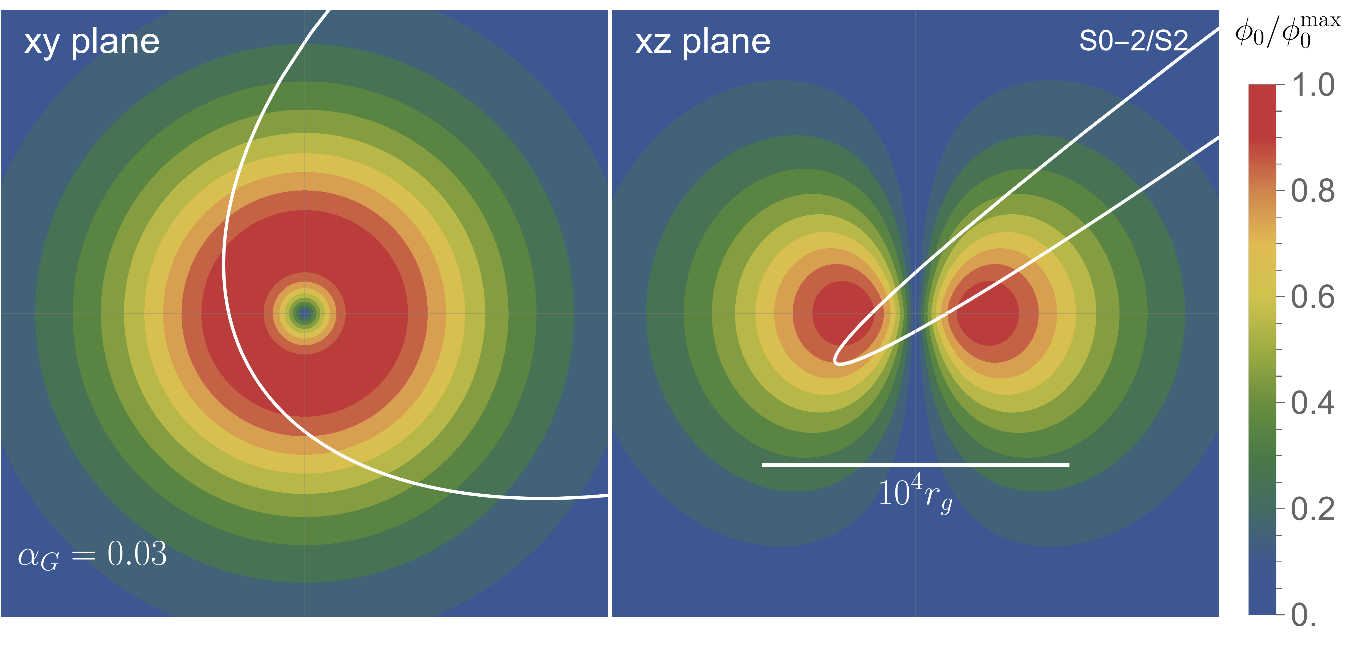
Since the scalar cloud wavefunction, Eq. (3.2), is anisotropic and aligned with the BH spin axis, it is necessary to analyze S-star orbits in the BH reference frame. We follow the procedure of Ref. [87] to transform the orbital motion into the BH frame, as detailed in Supplemental Material. This transformation requires the BH inclination angle $i_{\rm BH}$ and spin-projection position angle $\Omega_{\rm BH}$ . We adopt

i_{\rm BH}=155^{\circ}\pm 5^{\circ},\qquad\Omega_{\rm BH}=177^{\circ}\pm 25^{\circ},

(4.7)

obtained from fits to hotspot motion [74], consistent with previous GRAVITY and EHT measurements [88, 81]. The orbit of S0-2/S2, one of the closest and best-characterized S-stars, is shown as the white curve in Fig. 1, based on the fiducial values.

We first consider the Gemini/NIFS observations of S0-2/S2 during its pericenter passage in 2017 and 2018 [90]. Since the cloud wavefunction decays exponentially for $r\gg 1/(\mu\alpha_{G})$ , the strongest spectroscopic signals arise near periastron for highly eccentric orbits. The finite exposure time of approximately 10 minutes restricts the accessible parameter space to $\alpha_{G}\lesssim 0.055$ .

The projected constraints on $|C_{\gamma}|$ are shown in Fig. 2, with details provided in Supplemental Material. The exclusion curve exhibits a shallow minimum below $|C_{\gamma}|=1$ , reflecting the $\alpha_{G}^{2}$ suppression in Eq. (3.5) at lower masses and the decreasing overlap with the peak cloud density at larger masses. The black curve corresponds to the central values of $i_{\rm BH}$ and $\Omega_{\rm BH}$ , while the gray band indicates the associated uncertainties, which have only a minor impact on the overall sensitivity. For comparison, we also show the SN1987A constraint $\Lambda\equiv f_{\phi}/|C_{\gamma}|^{1/2}\gtrsim 3~{\rm TeV}$ [7], displayed on the right-hand axis and related to the left-hand axis for a fixed value of $f_{\phi}$ .

In Fig. 2, we also present a future projection that includes a late-type star with one-tenth the semi-major axis of S0-2/S2 and a similar eccentricity of $0.8$ , orbiting in the equatorial plane of the BH, with a total observation duration $10$ times longer than the data collected for S0-2/S2 in 2017 and 2018. The extension of the upper mass reach by a factor of two $(\alpha\lesssim 0.11)$ is enabled by the improved observational cadence, while the enhanced sensitivity is driven primarily by the anticipated three-order-of-magnitude improvement in spectral resolution.

Reaching sensitivities of $|C_{\gamma}|\sim 3\times 10^{-5}$ would begin to probe the QCD axion parameter space for decay constants not already excluded by SMBH spin measurements, namely $f_{\phi}\lesssim 10^{16}$ GeV, where such values can arise naturally in models with a $\mathbb{Z}_{N}$ symmetry [41]. We note, however, that QCD axions in this mass range are already subject to strong constraints from axion-potential flipping in dense nucleon environments [96, 97, 98, 99, 52]. Even for generic ALPs with quadratic photon couplings, higher-order effects can induce ALP–nucleon interactions that restrict the viable range of $f_{\phi}$ . Such constraints may nevertheless be relaxed in the presence of additional sectors [100, 101].

We finally comment on the role of leading dimension-five axion couplings in superradiant clouds, compared with the quadratic photon coupling considered in this work. Although the dimension-six operator is formally suppressed by one additional power of the scalar field, this suppression is substantially reduced in a superradiant cloud, where the field amplitude can approach the symmetry-breaking scale. In the saturated regime, the quadratic signal carries only an additional factor of order $\phi_{0}/f_{\phi}\sim{\cal O}(\alpha_{G})$ relative to a linear coupling, rather than an arbitrarily small perturbative suppression.

For the QCD axion, the dominant dimension-five interaction is the gluonic coupling, which induces an oscillating effective $\theta$ angle and hence time-dependent hadron and meson masses [20]. In practice, however, these effects leave much weaker and less distinctive imprints on stellar spectral lines than oscillations of $\alpha_{\rm EM}$ , and are considerably harder to isolate, since hadronic mass variations enter atomic spectra through multiple correlated quantities and are subject to significant degeneracies with stellar-atmosphere modeling, elemental abundances, and isotope-dependent effects. Similarly, a linear axion-photon coupling would primarily induce polarization rotation [129, 130, 131] rather than the spectroscopic modulation considered here. Its coefficient is controlled by an independent anomaly coefficient and is therefore not necessarily related to the quadratic photon coupling. Moreover, the achievable sensitivity is limited by polarization systematics, including uncertainties associated with propagation effects, magnetic-field modeling, and the intrinsic degree of linear polarization. For these reasons, the quadratic photon coupling provides a particularly clean and comparatively less degenerate observable.

4.2 Constraints from Soliton Core Dark Matter

We finally consider projected constraints on soliton core dark matter, as shown in Fig. 3. We present limits on $1/\Lambda$ (right $y$ -axis) for a generic quadratic scalar coupling and on $1/f_{\phi}$ (left $y$ -axis) assuming the benchmark value $|C_{\gamma}|=|C_{\gamma}^{\rm QCD}|\simeq 3\times 10^{-5}$ generated by an axion-gluon coupling.

For $\mu\lesssim 10^{-18}$ eV, the soliton core extends over parsec scales and encompasses the entire observed S-star cluster. Combined with the large field of view of future facilities, this enables simultaneous observations of approximately $40$ stars within a single coherent dark matter configuration. The coherent nature of the soliton core naturally facilitates a network of correlated spectroscopic measurements, in which multiple stars and multiple spectral lines can be analyzed jointly to search for a common oscillatory signal. This coherence provides a unique advantage by allowing many spatially separated stellar probes to sample the same high-density dark matter configuration.

For comparison, we also show existing terrestrial constraints on oscillations of the fine-structure constant, displayed as solid curves, including atomic-clock measurements [24, 26, 25, 102, 103, 104] and fifth-force/equivalence-principle-violation (EPV) tests [105, 50, 43]. These EPV bounds have recently been refined to incorporate momentum-dependent effects arising from couplings to nucleons [112, 111]. We also include a future projection from HISPEC/MODHIS, assuming a setup similar to that of Fig. 2 but incorporating simultaneous observations of $40$ late-type stars. This configuration is expected to achieve comparable sensitivity at higher frequencies, providing complementary reach under conservative assumptions for the dark matter distribution.

Additional constraints arising from axion-gluon couplings are shown as dashed curves, including limits from SN1987A [106], nuclear-parameter oscillations [20, 110, 101, 113], neutron electric dipole moment (nEDM) searches [107, 108, 109], and nuclear EPV tests [111]. Additionally, cosmological constraints from Big Bang nucleosynthesis [114, 46] and limits arising from nucleon environment backreaction [96, 97, 98, 99, 115] provide further restrictions on the parameter space. Figure 3 focuses on laboratory and astrophysical constraints, while relic-abundance considerations depend on the underlying cosmological history and are not shown.

5 Discussion

The environment near an SMBH at the Galactic Center can host extremely dense populations of ultralight bosons. Two representative scenarios are (i) BH superradiance, which exponentially amplifies a bound boson condensate and can drive the axion field to saturation near its decay constant, and (ii) ultralight DM forming a soliton core. The large field amplitudes in both cases substantially enhance axion-induced observables relative to terrestrial DM searches, making this system particularly sensitive to loop-induced interactions such as quadratic axion/scalar couplings to photons. In this work, we simulated precision spectroscopic measurements of S-stars orbiting Sgr A^∗ to probe these couplings, considering axion profiles sourced by either a superradiant cloud or a soliton core. Current data already demonstrate sensitivity to sizable regions of parameter space, while near-future improvements in spectroscopic sensitivity promise substantially broader coverage. Beyond Sgr A^∗, our framework applies to other BHs with companion stars or line-emitting plasma environments, enabling probes over many decades of scalar mass, including regimes relevant to vanilla QCD axions. Achieving this broader reach will require improved observational cadence, and the secular modulation of the bosonic cloud [116, 117, 118] provides an additional probe of higher-mass regimes that complements sensitivity to rapid oscillatory signals.

While we focused on the Newtonian $(2,1,1)$ superradiant mode, other cloud profiles are also relevant. At larger $\alpha_{G}$ , relativistic corrections become important and the $(3,2,2)$ mode may dominate the cloud mass and spatial extent, increasing stellar coverage [67, 71]. Additional possibilities include spherical $(1,0,0)$ gravitational atoms formed from DM relaxation [119, 36, 37], as well as gravitational molecules corotating with comparable-mass binaries [120, 121, 122, 123, 124, 125, 126]. These systems span diverse mass ranges and may exhibit nonlinear phenomena such as bosenova [127, 128, 36, 37, 69, 70]. Spectroscopic observations offer a novel means of visualizing these dynamics, effectively enabling tomographic reconstruction of the evolving bosonic wavefunction.

A range of complementary observations can further elucidate both macroscopic cloud properties and microscopic axion couplings. Axions with linear photon couplings rotate the plane of linear polarization, allowing EHT measurements to probe the parameter $c\equiv g_{a\gamma}f_{\phi}$ once saturation is reached [129, 76, 130, 131, 40, 132]. Combined polarimetry and spectroscopy thus provide a pathway to testing the ultraviolet origin of axions, alongside BH spin measurements that constrain large decay constants [60, 133, 56, 134, 135, 136, 137, 138, 139, 140]. Finally, purely gravitational observables can calibrate the cloud morphology through measurements of the cloud mass [141, 142, 38, 143, 144, 145, 146].

Acknowledgments

We are grateful to Sebastian A. R. Ellis, Xucheng Gan, Stefan Gillessen, Yuxin Liu, Minyuan Jiang, Hyungjin Kim, Hidetoshi Omiya, Gilad Perez, Diogo Ribeiro, Matteo Sadun-Bordoni, Wolfram Ratzinger, Konstantin Springmann, Pham Ngoc Hoa Vuong, Sam Witte, Guan-Wen Yuan, Qiang Yuan, and Yue Zhao for useful discussions. The Center of Gravity is a Center of Excellence funded by the Danish National Research Foundation under grant No. 184. V.C. and Y.C. acknowledge support by VILLUM Foundation (grant no. VIL37766) and the DNRF Chair program (grant no. DNRF162) by the Danish National Research Foundation. V.C. is a Villum Investigator and a DNRF Chair. V.C. acknowledges financial support provided under the European Union’s H2020 ERC Advanced Grant “Black holes: gravitational engines of discovery” grant agreement no. Gravitas–101052587. Views and opinions expressed are however those of the author only and do not necessarily reflect those of the European Union or the European Research Council. Neither the European Union nor the granting authority can be held responsible for them. This project has received funding from the European Union’s Horizon 2020 research and innovation programme under the Marie Sklodowska-Curie grant agreement No 101007855 and No 101131233. Y.C. is supported by the Rosenfeld foundation in the form of an Exchange Travel Grant and by the COST Action COSMIC WISPers CA21106, supported by COST (European Cooperation in Science and Technology). IFAE is partially funded by the CERCA program of the Generalitat de Catalunya. X.X. is funded by the grant CNS2023-143767. Grant CNS2023-143767 funded by MICIU/AEI/10.13039/501100011033 and by European Union NextGenerationEU/PRTR. Y.C. and X.X. acknowledge the support of the Rosenfeld foundation and the European Consortium for Astroparticle Theory in the form of an Exchange Travel Grant. H.X. is supported by Fermi Forward Discovery Group, LLC under Contract No. 89243024CSC000002 with the U.S. Dept. of Energy, Office of Science, Office of High Energy Physics.

Supplemental Material: Probing Fundamental Constant Oscillation in the Galactic Center with S-Star Spectroscopy

Appendix A S-Star Orbits in the Black Hole Frame

This section provides details on how to specify the orbit of a star in the black hole (BH) frame, where the BH spin axis aligns with the $\hat{z}$ -axis, following the procedures outlined in Ref. [87].

The orbital motion is initially defined in the observer frame, where the $\hat{z}$ -axis points from the observer to the orbit, and the $\hat{x}$ -axis points to the north/declination, as illustrated in Fig. A.1. The orbit is characterized by six orbital elements:

•

The eccentricity $e$ and semi-major axis $a$ , which describe the size and shape of the orbit.
•

The inclination $i_{s}$ and the longitude of the ascending node $\Omega_{s}$ , which define the orientation of the orbital plane.
•

The argument of periapsis $\omega_{s}$ , which specifies the direction of the orbit’s closest approach to the BH.
•

The true anomaly $\nu_{s}$ , which indicates the phase of the star along its orbit.

In the observer frame, the orbital motion can be expressed as

\vec{r}_{s}=\frac{a(1-e^{2})}{1+e\cos\nu_{s}}\left(\cos\nu_{s}\,\hat{a}+\sin\nu_{s}\,\hat{b}\right),

(A.1)

where

\hat{a}\equiv\begin{pmatrix}-\cos\omega_{s}\sin\Omega_{s}-\sin\omega_{s}\cos\Omega_{s}\cos i_{s}\\ \cos\omega_{s}\cos\Omega_{s}-\sin\omega_{s}\sin\Omega_{s}\cos i_{s}\\ \sin\omega_{s}\sin i_{s}\end{pmatrix},\quad\hat{b}\equiv\begin{pmatrix}\sin\omega_{s}\sin\Omega_{s}-\cos\omega_{s}\cos\Omega_{s}\cos i_{s}\\ -\sin\omega_{s}\cos\Omega_{s}-\cos\omega_{s}\sin\Omega_{s}\cos i_{s}\\ \cos\omega_{s}\sin i_{s}\end{pmatrix}.

(A.2)

To transform into the BH frame, we first consider the BH spin direction $\hat{J}_{\rm BH}$ , represented by the blue arrow in Fig. A.1. This direction is specified by the inclination angle $i_{\rm BH}$ and the position angle $\Omega_{\rm BH}$ , expressed as

\hat{J}_{\rm BH}=\left(\sin i_{\rm BH}\cos\Omega_{\rm BH},\sin i_{\rm BH}\sin\Omega_{\rm BH},\cos i_{\rm BH}\right).

(A.3)

To align $\hat{J}_{\rm BH}$ with the $\hat{z}$ -axis in the BH frame, we introduce a rotation matrix $\mathcal{R}_{\rm BH}$ :

\mathcal{R}_{\rm BH}=\begin{pmatrix}\sin\Omega_{\rm BH}&-\cos\Omega_{\rm BH}&0\\ \cos i_{\rm BH}\cos\Omega_{\rm BH}&\cos i_{\rm BH}\sin\Omega_{\rm BH}&-\sin i_{\rm BH}\\ \sin i_{\rm BH}\cos\Omega_{\rm BH}&\sin i_{\rm BH}\sin\Omega_{\rm BH}&\cos i_{\rm BH}\end{pmatrix}.

(A.4)

Using this transformation matrix, the star’s orbit in the BH frame is given by

\vec{r}_{s,{\rm BH}}=\frac{a(1-e^{2})}{1+e\cos\nu_{s}}\left(\cos\nu_{s}\,\hat{a}_{\rm BH}+\sin\nu_{s}\,\hat{b}_{\rm BH}\right),

(A.5)

where

\hat{a}_{\rm BH}=\mathcal{R}_{\rm BH}\hat{a}=\begin{pmatrix}-\cos\omega_{s}\cos(\Omega_{\rm BH}-\Omega_{s})-\cos i_{s}\sin\omega_{s}\sin(\Omega_{\rm BH}-\Omega_{s})\\ \cos i_{\rm BH}\left[\cos\omega_{s}\sin(\Omega_{\rm BH}-\Omega_{s})-\cos i_{s}\sin\omega_{s}\cos(\Omega_{\rm BH}-\Omega_{s})\right]-\sin i_{\rm BH}\sin i_{s}\sin\omega_{s}\\ \sin\omega_{s}\left[\cos i_{\rm BH}\sin i_{s}-\sin i_{\rm BH}\cos i_{s}\cos(\Omega_{\rm BH}-\Omega_{s})\right]+\sin i_{\rm BH}\cos\omega_{s}\sin(\Omega_{\rm BH}-\Omega_{s})\end{pmatrix},

(A.6)

and

\hat{b}_{\rm BH}=\mathcal{R}_{\rm BH}\hat{b}=\begin{pmatrix}\sin\omega_{s}\cos(\Omega_{\rm BH}-\Omega_{s})-\cos i_{s}\cos\omega_{s}\sin(\Omega_{\rm BH}-\Omega_{s})\\ -\cos i_{\rm BH}\left[\sin\omega_{s}\sin(\Omega_{\rm BH}-\Omega_{s})+\cos i_{s}\cos\omega_{s}\cos(\Omega_{\rm BH}-\Omega_{s})\right]-\sin i_{\rm BH}\cos i_{s}\sin\Omega_{s}\\ -\sin i_{\rm BH}\left[\sin\omega_{s}\sin(\Omega_{\rm BH}-\Omega_{s})+\cos i_{s}\cos\omega_{s}\cos(\Omega_{\rm BH}-\Omega_{s})\right]+\cos i_{\rm BH}\cos i_{s}\sin\Omega_{s}\end{pmatrix}.

(A.7)

Appendix B Statistics/Data Analysis

B.1 Data analysis

The data consists of spectroscopic measurements indexed by $I$ (star), $n$ (night), and $i$ (exposure). The measured data $d_{I,n,i}$ includes contributions from a potential signal $s_{I,n,i}(\bm{\Theta})$ (dependent on parameters $\bm{\Theta}$ ) and Gaussian noise $n_{I,n,i}\sim\mathcal{N}(0,\sigma_{I,n,i}^{2})$ . The likelihood function is given by:

\ln\mathcal{L}(\bm{\Theta}|\{d\})=-\frac{1}{2}\sum_{I,n,i}\left(\frac{d_{I,n,i}-s_{I,n,i}(\bm{\Theta})}{\sigma_{I,n,i}}\right)^{2}+\text{constant}.

(B.1)

For a signal model linear in parameters ( $s_{a}=\sum_{\mu}\mathcal{P}_{a,\mu}\Theta_{\mu}$ , where $a\equiv\{I,n,i\}$ ), the maximum likelihood estimate is obtained by solving:

\frac{\partial}{\partial\Theta_{\mu}}\ln\mathcal{L}(\bm{\Theta}|\{d\})=0,

(B.2)

yielding:

\displaystyle\bm{\Theta}_{\rm best-fit}=(\mathcal{P^{\prime}}^{T}\mathcal{P^{\prime}})^{-1}\mathcal{P^{\prime}}^{T}\bm{b},\quad\text{where }\ b_{a}\equiv\frac{d_{a}}{\sigma_{a}},\quad\mathcal{P}^{\prime}_{a,\mu}\equiv\frac{1}{\sigma_{a}}\mathcal{P}_{a,\mu}

(B.3)

Under the null hypothesis, mock data $d^{\rm mock}_{a}$ are generated as:

d^{\rm mock}_{a}=n_{a},\quad n_{a}\sim\mathcal{N}(0,\sigma_{a}^{2}).

(B.4)

The marginalized posterior distribution of $\Theta_{\rm best-fit,\mu}^{\rm mock}$ derived from mock data follows:

\Theta_{\rm best-fit,\mu}^{\rm mock}\sim\mathcal{N}\left(0,\sigma_{\Theta_{\mu}}^{2}\right),\quad\text{with }\sigma_{\Theta_{\mu}}^{2}=\left[(\mathcal{P}^{\prime T}\mathcal{P}^{\prime})^{-1}\right]_{\mu\mu},

(B.5)

where $\sigma_{\Theta_{\mu}}$ is the theoretical uncertainty from the Fisher information matrix $\mathcal{I}=\mathcal{P}^{\prime T}\mathcal{P}^{\prime}$ .

An $x\%$ confidence level exclusion limit $\Theta_{\mu}^{\rm up}$ is defined as the value satisfying:

P\left(\Theta_{\rm best-fit,\mu}\geq\Theta_{\mu}^{\rm up}\,|\,\Theta_{\mu}^{\rm true}=\Theta_{\mu}^{\rm up}\right)=(1-x)\%.

(B.6)

For Gaussian-distributed $\Theta_{\rm best-fit,\mu}$ , this corresponds to the $(1-x)\%$ quantile of the $\mathcal{N}(0,\sigma_{\Theta_{\mu}}^{2})$ distribution.

B.2 Signal modeling

From the main part of the paper, the spectroscopic signal due to ALP is

\frac{\delta\lambda_{j}}{\lambda_{j}}=-k_{\alpha,j}\frac{\delta\alpha_{\rm EM}}{\alpha_{\rm EM}}=-k_{\alpha,j}C_{\gamma}\frac{\phi^{2}}{f_{\phi}^{2}}\,,

(B.7)

where the subscript $j$ refers to a particular atomic line, $k_{\alpha,j}$ is the sensitivity of the atomic transition to the fine structure constant (typically $\sim 2$ for H atomic lines).

Using the solution for the ALP scalar field $\phi$ provided in the main part of the paper, one finds that the signal can be written as


	$\displaystyle\frac{\delta\lambda}{\lambda}=s(t,\bm{x})$	$\displaystyle=-k_{\alpha}C_{\gamma}\frac{\left(\sin\theta\phi_{0}^{\mathrm{max}}R(r)\right)^{2}}{2f_{\phi}^{2}}\left[1+\cos 2(\mu t-\varphi)\cos 2\Delta_{0}-\sin 2(\mu t-\varphi)\sin 2\Delta_{0}\right]\,$	(B.8a)
		$\displaystyle=s_{0}(\bm{x})\Big[A\sin(2\mu t-2\varphi)+B\cos(2\mu t-2\varphi)\Big]+\cdots\,,$	(B.8b)
where $s_{0}(x)=k_{\alpha}\Big(\sin\theta\phi_{0}^{\mathrm{max}}R(r)\Big)^{2}/2$ , and the $\cdots$ denotes terms evolving on the orbital timescale, which are not considered in this analysis focused on rapid oscillations. Note that in the data analysis, it is better to infer the $2$ parameters $A$ and $B$ since the model is linear in these parameters and to convert the resulting posterior into a posterior on the coupling parameter using $C_{\gamma}/f_{\phi}^{2}=\sqrt{A^{2}+B^{2}}$ .

B.3 Example: Simplified Observational Scenario

Here, for pedagogical purposes, we give an example of a data analysis in a simplified observational scenario.

Consider a signal model of the form:

s(t,\bm{x})=s_{0}(\bm{x})\Big[A\sin(2\mu t-2\varphi)+B\cos(2\mu t-2\varphi)\Big]+k_{I,n},

(B.9)

where $k_{I,n}$ represents a night-specific instrumental systematic offset for the night $n$ . The free parameters are:

\bm{\Theta}=\{A,\,B,\,k_{I,n}\}.

(B.10)

We will consider a case where we observe 2 stars, with the following observation scheduling:

•
Star 1:
- –
  
  Night 1: 2 exposures (Obs a, Obs b)
- –
  
  Night 2: 1 exposure (Obs c)
•
Star 2:
- –
  
  Night 1: 1 exposure (Obs d)

This yields $4$ exposures and $5$ free parameters. The $\mathcal{P}^{\prime}$ -matrix (dimensions $4\times 5$ ) becomes:

\mathcal{P}^{\prime}=\begin{pmatrix}\dfrac{s_{0}(\bm{x}_{a})\sin\phi_{a}}{\sigma_{a}}&\dfrac{s_{0}(\bm{x}_{a})\cos\phi_{a}}{\sigma_{a}}&\dfrac{1}{\sigma_{a}}&0&0\\ \dfrac{s_{0}(\bm{x}_{b})\sin\phi_{b}}{\sigma_{b}}&\dfrac{s_{0}(\bm{x}_{b})\cos\phi_{b}}{\sigma_{b}}&\dfrac{1}{\sigma_{b}}&0&0\\ \dfrac{s_{0}(\bm{x}_{c})\sin\phi_{c}}{\sigma_{c}}&\dfrac{s_{0}(\bm{x}_{c})\cos\phi_{c}}{\sigma_{c}}&0&\dfrac{1}{\sigma_{c}}&0\\ \dfrac{s_{0}(\bm{x}_{d})\sin\phi_{d}}{\sigma_{d}}&\dfrac{s_{0}(\bm{x}_{d})\cos\phi_{d}}{\sigma_{d}}&0&0&\dfrac{1}{\sigma_{d}}\\ \end{pmatrix},

(B.11)

where $\phi_{i}\equiv 2\mu t_{i}-2\varphi$ , and subscripts $i=a,b,c,d$ denote observations (e.g., $\sigma_{a}=\sigma_{1,1,1}$ , $\bm{x}_{c}=\bm{x}_{1,2,1}$ ).

Appendix C Generation of Mock data

In this analysis, we explore two scenarios: (i) a case of existing data for the star S0-2/S2 and (ii) a case of futuristic measurements that will be performed using the next generation of instrument.

C.1 Existing data

We consider the spectroscopic measurements of the short period star S0-2/S2 during the 2017-2018 measurement campaign, when the star was going through its periastron. The dataset is presented in Ref. [90] (see Sec. $1.1$ from the Supplementary Materials of Ref. [90]). In 2017-2018, spectroscopic data has been taken from three instruments: (i) OSIRIS at the Keck observatory, (ii) IRCS at the SUBARU telescope and (iii) NISF from the Gemini observatory.

Each night of observation, several frames of integration time between 300 and 900 s are taken. In Ref. [90], all the frames for each night are combined together to produce a daily estimate of the star radial velocity (RV). In this analysis, since we are interested in measuring fast oscillations in the spectroscopic measurements such that it is more powerful to work directly with individual frames. This would require a detailed re-analysis of all raw data presented in Sec. $1.1$ from the Supplementary Materials of Ref. [90], which is beyond the scope of our sensitivity analysis.

In order to perform our sensitivity analysis, we need to have a realistic estimate of the expected uncertainty of the spectroscopic measurement for each individual frame. In this sensitivity analysis, we use one night of data from the Gemini NIFS instrument and assume that the characteristic instrumental noise is representative of all spectroscopic measurements conducted between 2017 and 2019 across various instruments. Specifically, we consider the Gemini NIFS dataset from 2018-05-13, which is part of the data presented in Ref. [90], consisting of 12 frames with 600 s integration time each. Of the 12 frames, only 8 of the individual data points were useful for individual relative RV measurements. The relative spectroscopic measurement is obtained by cross-correlating each individual spectrum with a combined spectrum of the night. For simplicity, we only used the Hydrogen line at 2.1661 microns (Br- $\gamma$ ). The individual extracted data is presented in Fig. C.1. The median RV uncertainty is $28$ km/s and the RV scatter throughout the night is about $24$ km/s, which is consistent with the uncertainties. The results can be sensitive to how the spectra are extracted and correlated so this could be refined in the future.

In our analysis, we generated a mock dataset for 2017-2018 using the characteristic of the measurement noise from the night 2018-05-13. Specifically, we assume that 25 % of the frames will not be usable and we draw the RV uncertainty for each frame from a probability distribution that has been fitted to the distribution of the RV distribution from Fig. C.1; namely, $(\sigma_{\mathrm{RV}}-10\,\mathrm{km/s})/10\,\mathrm{km/s}$ is modeled by a Gamma distribution with shape parameter $3$ .

C.2 Future data

In our analysis, we also simulated data that would be representative of future instruments such as HISPEC and MODHIS [94, 95]. With these instruments, we expect a three-order-of-magnitude improvement in spectroscopic resolution, a halved cadence [94, 95]. Such instruments would also enable the detection of late-type stars. With cooler atmospheres, these stars exhibit a rich variety of spectral lines with smaller intrinsic variance, in contrast to hot, early-type stars like S0-2/S2. Thus, we assume a reduction of $\sigma_{\mathrm{RV}}$ by a factor of $10^{3}$ .

We generate mock data incorporating these instrumental properties and spanning a time baseline ten times longer than the current dataset. To probe superradiant clouds, we consider a hypothetical late-type star with a semi-major axis equal to 10% that of S0-2/S2, which would yield a significantly larger signal due to its closer proximity to the BH. For soliton-core dark matter, we assume simultaneous spectroscopic observations of $40$ stars within both the telescope’s field of view and the spatial extent of the soliton core.

Appendix D Plasma Effects

A key question is whether the scalar cloud can continue to grow once corrections to the fine-structure constant become sizable. In vacuum, when the scalar field approaches the cutoff scale $\Lambda$ , parametric annihilation into photons can efficiently deplete the cloud. In the astrophysical environment considered here, however, the photon plasma mass $\omega_{p}$ is several orders of magnitude larger than the scalar masses of interest, kinematically suppressing such annihilation channels. As a result, the dominant dissipation mechanism becomes plasma heating, analogous to constraints on low-mass dark photon dark matter [92].

We consider the quadratic coupling $\phi^{2}F_{\mu\nu}F^{\mu\nu}/(4\Lambda^{2})$ and focus on the perturbative regime, where the induced variation of the fine-structure constant is small,

\frac{\delta\alpha_{\rm EM}}{\alpha_{\rm EM}}\sim\frac{\phi_{0}^{2}}{\Lambda^{2}}\equiv\varepsilon\ll 1.

(D.1)

Expanding around the background field $\phi=\phi_{0}+\delta\phi$ , and considering a background magnetic field $\vec{B}_{0}$ and a transverse photon mode $A_{T}$ in a plasma, the linearized equations of motion in Fourier space $(\omega,\vec{k})$ read

\left[\vec{k}^{\,2}-\omega^{2}+\begin{pmatrix}\Omega_{p}^{2}&\omega\,\dfrac{\phi_{0}}{\Lambda^{2}}B_{0}\\ \omega\,\dfrac{\phi_{0}}{\Lambda^{2}}B_{0}&\mu^{2}\end{pmatrix}\right]\begin{pmatrix}A_{T}\\ \delta\phi\end{pmatrix}=0\,,

(D.2)

where $B_{0}\equiv|\vec{B}_{0}|$ . The complex plasma frequency is

\Omega_{p}^{2}\equiv\frac{\omega_{p}^{2}}{1+i\nu/\omega},\qquad\omega_{p}^{2}=\frac{4\pi\alpha_{\rm EM}n_{e}}{m_{e}},

(D.3)

with $n_{e}$ and $m_{e}$ the electron number density and mass. The electron–ion collision rate governing collisional damping is

\nu=\frac{4\sqrt{2\pi}\,\alpha_{\rm EM}^{2}\,n_{e}}{3m_{e}^{1/2}T_{e}^{3/2}}\log\Lambda_{C}\;\simeq\;2\times 10^{-23}~{\rm eV}\left(\frac{n_{e}}{10~{\rm cm}^{-3}}\right)\left(\frac{10^{7}~{\rm K}}{T_{e}}\right)^{3/2},

(D.4)

where we take the Coulomb logarithm $\log\Lambda_{C}\simeq 30$ , and $T_{e}$ denotes the electron temperature.

Diagonalizing the $2\times 2$ system in Eq. (D.2) for small mixing and in the non-relativistic limit for the scalar ( $|\vec{k}|\ll\omega\simeq\mu$ ), with $\mu\ll\omega_{p}$ , one finds that the scalar eigenfrequency acquires an imaginary part inherited from the photon, corresponding to a damping rate

\gamma_{\phi}^{\rm(plasma)}\;\simeq\;\frac{\phi_{0}^{2}}{\Lambda^{4}}\,\frac{B_{0}^{2}\,\nu}{2\omega_{p}^{2}}.

(D.5)

For the superradiant cloud considered in our work, the relevant region lies at radii $r\gtrsim 100~r_{g}$ , where the plasma is relatively dilute and the magnetic field corresponds to the large-scale Galactic Center environment rather than the near-horizon region. As representative values we take [93, 147, 148]

n_{e}\sim 10~{\rm cm}^{-3},\qquad T_{e}\sim 10^{7}~{\rm K},\qquad B_{0}\sim 1~{\rm mG}.

(D.6)

These parameters yield $\nu\sim 2\times 10^{-23}~{\rm eV}$ and $\omega_{p}\sim 1\times 10^{-10}~{\rm eV}$ .

Imposing the perturbative condition $\phi_{0}^{2}/\Lambda^{2}=\varepsilon\ll 1$ and the current constraint $\Lambda\gtrsim 3~{\rm TeV}$ , we obtain a conservative upper bound on the scalar cloud decay rate due to plasma heating,

\gamma_{\phi}^{\rm(plasma)}\;\lesssim\;\frac{1}{\Lambda^{2}}\frac{B_{0}^{2}\,\nu}{2\omega_{p}^{2}}\;\sim\;3\times 10^{-38}~{\rm eV}.

(D.7)

In our analysis, the mass windows of interest require the superradiant growth rate to exceed the inverse age of the Universe,

\Gamma_{\rm SR}\gtrsim 10^{-32}~{\rm eV}.

(D.8)

Therefore, even in the most conservative perturbative limit, $\gamma_{\phi}^{\rm(plasma)}\ll\Gamma_{\rm SR}$ , and collisional plasma heating cannot halt or significantly modify the exponential growth of the superradiant cloud. Consequently, the superradiant mass window remains unchanged.

We now consider the regime in which the scalar background continues to grow and the induced correction to the fine-structure constant becomes comparable to, or larger than, the vacuum contribution, while remaining below the fully nonperturbative QED limit $\delta\alpha_{\rm EM}\sim\mathcal{O}(1)$ . For a superradiant cloud, this occurs only when $|C_{\gamma}|=f_{\phi}^{2}/\Lambda^{2}\gg 1$ . In this regime, the scalar evolution is still adiabatic compared to electromagnetic and plasma timescales, so the electromagnetic sector responds quasi-instantaneously to a slowly varying, scalar-dominated coupling.

Once $\alpha_{\rm EM}$ is no longer dominated by its vacuum value, plasma effects are significantly enhanced. In particular, the electron–ion collision rate and other dissipative processes increase with the effective electromagnetic coupling, while the photon plasma mass is also modified accordingly. As a consequence, plasma heating becomes increasingly efficient. This enhanced dissipation rapidly transfers energy from the scalar cloud into the plasma and leads to a saturation of the cloud configuration, in which the superradiant energy injection is balanced by plasma dissipation.

In this regime, the fine-structure constant exhibits adiabatic oscillations with amplitudes substantially larger than those allowed in vacuum. Such stable and large variations are already strongly constrained by the observed stability of atomic and molecular spectral lines in the Galactic Center.

For the scalar mass window, the region satisfying the superradiant condition and a sufficiently rapid growth rate remains the one constrained by our analysis, since the saturation phase extracts BH rotational energy linearly and induces only minor gravitational backreaction. Stronger coupling at smaller $\Lambda$ could marginally extend the low-mass end by reducing the threshold field value for saturation; for conservativeness, we do not include this possible extension.

On the other hand, a strong background magnetic field $B_{0}$ can modify superradiant dynamics by inducing an effective scalar mass through the quadratic interaction,

\mu_{\rm eff}^{2}\;=\;\mu^{2}+\Delta\mu^{2},\qquad\Delta\mu^{2}\sim\frac{B_{0}^{2}}{\Lambda^{2}}\;\simeq\;\left(6\times 10^{-18}\,\mathrm{eV}\right)^{2}\left(\frac{B_{0}}{1~\mathrm{mG}}\right)^{2}\left(\frac{3~\mathrm{TeV}}{\Lambda}\right)^{2},

(D.9)

up to order-unity geometric factors.

Superradiance is governed by the effective scalar mass $\mu_{\rm eff}$ rather than the bare mass $\mu$ . Accordingly, the superradiant condition and the associated growth rate should be evaluated using $\mu_{\rm eff}$ . If $\mu_{\rm eff}$ falls within the superradiant window probed in our analysis, then scalar masses below the nominal lower edge of the vacuum mass window can also be excluded, since the enhanced effective mass shortens the superradiant timescale and enables efficient cloud growth. Conversely, if the induced effective mass exceeds the upper boundary of the superradiant window, set by the superradiant condition and observational cadence limitations, no additional constraint can be obtained, leading instead to a cutoff of the exclusion region at large coupling.

As seen from Eq. (D.9), for Galactic Center magnetic fields at the mG level and $\Lambda$ near the current bound of $3~\mathrm{TeV}$ , the induced effective mass lies within the mass range relevant to this study. Consequently, its impact on the exclusion region in Fig. 2 introduces a cutoff near the upper edge of the constrained parameter space. The same applies to the soliton-core dark matter scenario, where only the uppermost region is modified.

References

[1] J. Preskill, M. B. Wise and F. Wilczek, Cosmology of the Invisible Axion, Phys. Lett. B 120 (1983) 127–132.
[2] L. F. Abbott and P. Sikivie, A Cosmological Bound on the Invisible Axion, Phys. Lett. B 120 (1983) 133–136.
[3] M. Dine and W. Fischler, The Not So Harmless Axion, Phys. Lett. B 120 (1983) 137–141.
[4] P. Svrcek and E. Witten, Axions In String Theory, JHEP 06 (2006) 051, [hep-th/0605206].
[5] A. Arvanitaki, S. Dimopoulos, S. Dubovsky, N. Kaloper and J. March-Russell, String Axiverse, Phys. Rev. D 81 (2010) 123530, [0905.4720].
[6] J.-P. Uzan, The Fundamental Constants and Their Variation: Observational Status and Theoretical Motivations, Rev. Mod. Phys. 75 (2003) 403, [hep-ph/0205340].
[7] K. A. Olive and M. Pospelov, Environmental dependence of masses and coupling constants, Phys. Rev. D 77 (2008) 043524, [0709.3825].
[8] J.-P. Uzan, Varying Constants, Gravitation and Cosmology, Living Rev. Rel. 14 (2011) 2, [1009.5514].
[9] Y. V. Stadnik and V. V. Flambaum, Can dark matter induce cosmological evolution of the fundamental constants of Nature?, Phys. Rev. Lett. 115 (2015) 201301, [1503.08540].
[10] C. J. A. P. Martins, The status of varying constants: a review of the physics, searches and implications, 1709.02923.
[11] M. S. Safronova, D. Budker, D. DeMille, D. F. J. Kimball, A. Derevianko and C. W. Clark, Search for New Physics with Atoms and Molecules, Rev. Mod. Phys. 90 (2018) 025008, [1710.01833].
[12] J.-P. Uzan, Fundamental constants: from measurement to the universe, a window on gravitation and cosmology, 2410.07281.
[13] T. R. Taylor and G. Veneziano, Dilaton Couplings at Large Distances, Phys. Lett. B 213 (1988) 450–454.
[14] T. Damour and A. M. Polyakov, String theory and gravity, Gen. Rel. Grav. 26 (1994) 1171–1176, [gr-qc/9411069].
[15] I. Antoniadis, N. Arkani-Hamed, S. Dimopoulos and G. R. Dvali, New dimensions at a millimeter to a Fermi and superstrings at a TeV, Phys. Lett. B 436 (1998) 257–263, [hep-ph/9804398].
[16] T. Damour and J. F. Donoghue, Phenomenology of the Equivalence Principle with Light Scalars, Class. Quant. Grav. 27 (2010) 202001, [1007.2790].
[17] T. Damour and J. F. Donoghue, Equivalence Principle Violations and Couplings of a Light Dilaton, Phys. Rev. D 82 (2010) 084033, [1007.2792].
[18] P. W. Graham, D. E. Kaplan and S. Rajendran, Cosmological Relaxation of the Electroweak Scale, Phys. Rev. Lett. 115 (2015) 221801, [1504.07551].
[19] T. Flacke, C. Frugiuele, E. Fuchs, R. S. Gupta and G. Perez, Phenomenology of relaxion-Higgs mixing, JHEP 06 (2017) 050, [1610.02025].
[20] H. Kim and G. Perez, Oscillations of atomic energy levels induced by QCD axion dark matter, Phys. Rev. D 109 (2024) 015005, [2205.12988].
[21] C. Beadle, S. A. R. Ellis, J. Quevillon and P. N. Hoa Vuong, Quadratic coupling of the axion to photons, Phys. Rev. D 110 (2024) 035019, [2307.10362].
[22] H. Kim, A. Lenoci, G. Perez and W. Ratzinger, Probing an ultralight QCD axion with electromagnetic quadratic interaction, Phys. Rev. D 109 (2024) 015030, [2307.14962].
[23] A. Arvanitaki, J. Huang and K. Van Tilburg, Searching for dilaton dark matter with atomic clocks, Phys. Rev. D 91 (2015) 015015, [1405.2925].
[24] K. Van Tilburg, N. Leefer, L. Bougas and D. Budker, Search for ultralight scalar dark matter with atomic spectroscopy, Phys. Rev. Lett. 115 (2015) 011802, [1503.06886].
[25] A. Hees, J. Guéna, M. Abgrall, S. Bize and P. Wolf, Searching for an oscillating massive scalar field as a dark matter candidate using atomic hyperfine frequency comparisons, Phys. Rev. Lett. 117 (2016) 061301, [1604.08514].
[26] X. Zhang, A. Banerjee, M. Leyser, G. Perez, S. Schiller, D. Budker et al., Search for Ultralight Dark Matter with Spectroscopy of Radio-Frequency Atomic Transitions, Phys. Rev. Lett. 130 (2023) 251002, [2212.04413].
[27] Y. V. Stadnik and V. V. Flambaum, Searching for dark matter and variation of fundamental constants with laser and maser interferometry, Phys. Rev. Lett. 114 (2015) 161301, [1412.7801].
[28] Y. V. Stadnik and V. V. Flambaum, Enhanced effects of variation of the fundamental constants in laser interferometers and application to dark matter detection, Phys. Rev. A 93 (2016) 063630, [1511.00447].
[29] A. Branca et al., Search for an Ultralight Scalar Dark Matter Candidate with the AURIGA Detector, Phys. Rev. Lett. 118 (2017) 021302, [1607.07327].
[30] W. M. Campbell, B. T. McAllister, M. Goryachev, E. N. Ivanov and M. E. Tobar, Searching for Scalar Dark Matter via Coupling to Fundamental Constants with Photonic, Atomic and Mechanical Oscillators, Phys. Rev. Lett. 126 (2021) 071301, [2010.08107].
[31] S. M. Vermeulen et al., Direct limits for scalar field dark matter from a gravitational-wave detector, 2103.03783.
[32] A. Hees et al., Search for a Variation of the Fine Structure Constant around the Supermassive Black Hole in Our Galactic Center, Phys. Rev. Lett. 124 (2020) 081101, [2002.11567].
[33] R. Penrose and R. M. Floyd, Extraction of rotational energy from a black hole, Nature 229 (1971) 177–179.
[34] Y. B. Zel’Dovich, Generation of Waves by a Rotating Body, Soviet Journal of Experimental and Theoretical Physics Letters 14 (Aug., 1971) 180.
[35] R. Brito, V. Cardoso and P. Pani, Superradiance: New Frontiers in Black Hole Physics, Lect. Notes Phys. 906 (2015) pp.1–237, [1501.06570].
[36] D. Budker, J. Eby, M. Gorghetto, M. Jiang and G. Perez, A generic formation mechanism of ultralight dark matter solar halos, JCAP 12 (2023) 021, [2306.12477].
[37] X. Gan, L.-T. Wang and H. Xiao, Detecting axion dark matter with black hole polarimetry, Phys. Rev. D 110 (2024) 063039, [2311.02149].
[38] Y. Chen, X. Xue, R. Brito and V. Cardoso, Photon Ring Astrometry for Superradiant Clouds, Phys. Rev. Lett. 130 (2023) 111401, [2211.03794].
[39] Y. Chen, X. Xue and V. Cardoso, Black holes as fermion factories, JCAP 02 (2025) 035, [2308.00741].
[40] D. Ayzenberg et al., Fundamental physics opportunities with future ground-based mm/sub-mm VLBI arrays, Living Rev. Rel. 28 (2025) 4, [2312.02130].
[41] A. Hook, Solving the Hierarchy Problem Discretely, Phys. Rev. Lett. 120 (2018) 261802, [1802.10093].
[42] Y. V. Stadnik and V. V. Flambaum, Improved limits on interactions of low-mass spin-0 dark matter from atomic clock spectroscopy, Phys. Rev. A 94 (2016) 022111, [1605.04028].
[43] A. Hees, O. Minazzoli, E. Savalle, Y. V. Stadnik and P. Wolf, Violation of the equivalence principle from light scalar dark matter, Phys. Rev. D 98 (2018) 064051, [1807.04512].
[44] A. Hees, O. Minazzoli, E. Savalle, Y. V. Stadnik, P. Wolf and B. Roberts, Violation of the equivalence principle from light scalar fields: from Dark Matter candidates to scalarized black holes, in 54th Rencontres de Moriond on Gravitation, 5, 2019, 1905.08524.
[45] H. Masia-Roig et al., Intensity interferometry for ultralight bosonic dark matter detection, Phys. Rev. D 108 (2023) 015003, [2202.02645].
[46] T. Bouley, P. Sørensen and T.-T. Yu, Constraints on ultralight scalar dark matter with quadratic couplings, JHEP 03 (2023) 104, [2211.09826].
[47] A. Banerjee, G. Perez, M. Safronova, I. Savoray and A. Shalit, The phenomenology of quadratically coupled ultra light dark matter, JHEP 10 (2023) 042, [2211.05174].
[48] X. Gan and D. Liu, Cosmologically varying kinetic mixing, JHEP 11 (2023) 031, [2302.03056].
[49] P. Brax, C. Burrage, J. A. R. Cembranos and P. Valageas, Invisible dilaton, Phys. Rev. D 107 (2023) 095015, [2303.14469].
[50] J. Bergé, P. Brax, G. Métris, M. Pernot-Borràs, P. Touboul and J.-P. Uzan, MICROSCOPE Mission: First Constraints on the Violation of the Weak Equivalence Principle by a Light Scalar Dilaton, Phys. Rev. Lett. 120 (2018) 141101, [1712.00483].
[51] P. Cox, M. J. Dolan and F. J. Hiskens, Photonic Freeze-In, 2412.17308.
[52] X. Gan, D. Liu, D. Liu, X. Luo and B. Yu, Detecting Ultralight Dark Matter with Matter Effect, 2504.11522.
[53] S. L. Detweiler, KLEIN-GORDON EQUATION AND ROTATING BLACK HOLES, Phys. Rev. D 22 (1980) 2323–2326.
[54] V. Cardoso and S. Yoshida, Superradiant instabilities of rotating black branes and strings, JHEP 07 (2005) 009, [hep-th/0502206].
[55] S. R. Dolan, Instability of the massive Klein-Gordon field on the Kerr spacetime, Phys. Rev. D 76 (2007) 084001, [0705.2880].
[56] R. Brito, V. Cardoso and P. Pani, Black holes as particle detectors: evolution of superradiant instabilities, Class. Quant. Grav. 32 (2015) 134001, [1411.0686].
[57] W. E. East and F. Pretorius, Superradiant Instability and Backreaction of Massive Vector Fields around Kerr Black Holes, Phys. Rev. Lett. 119 (2017) 041101, [1704.04791].
[58] C. A. R. Herdeiro, E. Radu and N. M. Santos, A bound on energy extraction (and hairiness) from superradiance, Phys. Lett. B 824 (2022) 136835, [2111.03667].
[59] Z.-H. Lyu, R.-G. Cai, Z.-K. Guo, J.-F. He and J. Liu, Ring formation from black hole superradiance through repeated particle production on bound orbits, 2507.03490.
[60] A. Arvanitaki and S. Dubovsky, Exploring the String Axiverse with Precision Black Hole Physics, Phys. Rev. D 83 (2011) 044026, [1004.3558].
[61] H. Yoshino and H. Kodama, Bosenova collapse of axion cloud around a rotating black hole, Prog. Theor. Phys. 128 (2012) 153–190, [1203.5070].
[62] A. Gruzinov, Black Hole Spindown by Light Bosons, 1604.06422.
[63] H. Fukuda and K. Nakayama, Aspects of Nonlinear Effect on Black Hole Superradiance, JHEP 01 (2020) 128, [1910.06308].
[64] M. Baryakhtar, M. Galanis, R. Lasenby and O. Simon, Black hole superradiance of self-interacting scalar fields, Phys. Rev. D 103 (2021) 095019, [2011.11646].
[65] H. Omiya, T. Takahashi and T. Tanaka, Renormalization group analysis of superradiant growth of self-interacting axion cloud, PTEP 2021 (2021) 043E02, [2012.03473].
[66] H. Omiya, T. Takahashi and T. Tanaka, Adiabatic evolution of the self-interacting axion field around rotating black holes, PTEP 2022 (2022) 043E03, [2201.04382].
[67] H. Omiya, T. Takahashi, T. Tanaka and H. Yoshino, Impact of multiple modes on the evolution of self-interacting axion condensate around rotating black holes, JCAP 06 (2023) 016, [2211.01949].
[68] S. Collaviti, L. Sun, M. Galanis and M. Baryakhtar, Observational prospects of self-interacting scalar superradiance with next-generation gravitational-wave detectors, Class. Quant. Grav. 42 (2025) 025006, [2407.04304].
[69] T. Takahashi, H. Omiya and T. Tanaka, Self-interacting axion clouds around rotating black holes in binary systems, Phys. Rev. D 110 (2024) 104038, [2408.08349].
[70] J. C. Aurrekoetxea, J. Marsden, K. Clough and P. G. Ferreira, Self-interacting scalar dark matter around binary black holes, Phys. Rev. D 110 (2024) 083011, [2409.01937].
[71] S. J. Witte and A. Mummery, Stepping up superradiance constraints on axions, Phys. Rev. D 111 (2025) 083044, [2412.03655].
[72] A. L. Miller, Gravitational wave probes of particle dark matter: a review, 2503.02607.
[73] N. Xie and F. P. Huang, The self-interaction effects on the Kerr black hole superradiance and their observational implications, 2503.10347.
[74] GRAVITY collaboration, R. Abuter et al., Polarimetry and astrometry of NIR flares as event horizon scale, dynamical probes for the mass of Sgr A*, Astron. Astrophys. 677 (2023) L10, [2307.11821].
[75] H.-Y. Schive, T. Chiueh and T. Broadhurst, Cosmic Structure as the Quantum Interference of a Coherent Dark Wave, Nature Phys. 10 (2014) 496–499, [1406.6586].
[76] G.-W. Yuan, Z.-Q. Xia, C. Tang, Y. Zhao, Y.-F. Cai, Y. Chen et al., Testing the ALP-photon coupling with polarization measurements of Sagittarius A^∗, JCAP 03 (2021) 018, [2008.13662].
[77] J. F. Navarro, C. S. Frenk and S. D. M. White, The Structure of cold dark matter halos, Astrophys. J. 462 (1996) 563–575, [astro-ph/9508025].
[78] H. Kim, A. Lenoci, I. Stomberg and X. Xue, Adiabatically compressed wave dark matter halo and intermediate-mass-ratio inspirals, Phys. Rev. D 107 (2023) 083005, [2212.07528].
[79] S. Gillessen, P. M. Plewa, F. Eisenhauer, R. Sari, I. Waisberg, M. Habibi et al., An update on monitoring stellar orbits in the galactic center, The Astrophysical Journal 837 (Feb., 2017) 30.
[80] GRAVITY collaboration, R. Abuter et al., Mass distribution in the Galactic Center based on interferometric astrometry of multiple stellar orbits, Astron. Astrophys. 657 (2022) L12, [2112.07478].
[81] Event Horizon Telescope collaboration, K. Akiyama et al., First Sagittarius A* Event Horizon Telescope Results. I. The Shadow of the Supermassive Black Hole in the Center of the Milky Way, Astrophys. J. Lett. 930 (2022) L12, [2311.08680].
[82] Event Horizon Telescope collaboration, K. Akiyama et al., First Sagittarius A* Event Horizon Telescope Results. V. Testing Astrophysical Models of the Galactic Center Black Hole, Astrophys. J. Lett. 930 (2022) L16, [2311.09478].
[83] Y. Wang and B. Zhang, Evidence of a past merger of the Galactic Centre black hole, Nature Astron. 8 (2024) 1592–1601, [2403.06416].
[84] Planck collaboration, N. Aghanim et al., Planck 2018 results. VI. Cosmological parameters, Astron. Astrophys. 641 (2020) A6, [1807.06209].
[85] D. Baumann, H. S. Chia and R. A. Porto, Probing Ultralight Bosons with Binary Black Holes, Phys. Rev. D 99 (2019) 044001, [1804.03208].
[86] V. Cardoso, F. Duque and T. Ikeda, Tidal effects and disruption in superradiant clouds: a numerical investigation, Phys. Rev. D 101 (2020) 064054, [2001.01729].
[87] M. Grould, F. H. Vincent, T. Paumard and G. Perrin, General relativistic effects on the orbit of the S2 star with GRAVITY, Astron. Astrophys. 608 (2017) A60, [1709.04492].
[88] GRAVITY collaboration, R. Abuter et al., Detection of orbital motions near the last stable circular orbit of the massive black hole sgra*, Astron. Astrophys. 618 (Oct., 2018) L10.
[89] D. S. Chu et al., Investigating the Binarity of S0-2: Implications for its Origins and Robustness as a Probe of the Laws of Gravity around a Supermassive Black Hole, Astrophys. J. 854 (2018) 12, [1709.04890].
[90] T. Do et al., Relativistic redshift of the star S0-2 orbiting the Galactic center supermassive black hole, Science 365 (2019) 664–668, [1907.10731].
[91] G.-W. Yuan, Z.-Q. Shen, Y.-L. S. Tsai, Q. Yuan and Y.-Z. Fan, Constraining ultralight bosonic dark matter with Keck observations of S2’s orbit and kinematics, Phys. Rev. D 106 (2022) 103024, [2205.04970].
[92] S. Dubovsky and G. Hernández-Chifflet, Heating up the Galaxy with Hidden Photons, JCAP 12 (2015) 054, [1509.00039].
[93] R. M. Crocker, D. I. Jones, F. Melia, J. Ott and R. J. Protheroe, A lower limit of 50 microgauss for the magnetic field near the galactic centre, Nature 463 (Jan., 2010) 65–67.
[94] D. Mawet et al., High-resolution Infrared Spectrograph for Exoplanet Characterization with the Keck and Thirty Meter Telescopes, 1908.03623.
[95] Q. M. Konopacky et al., The development of HISPEC for Keck and MODHIS for TMT: science cases and predicted sensitivities, in Techniques and Instrumentation for Detection of Exoplanets XI (G. J. Ruane, ed.), vol. 12680, p. 1268007, International Society for Optics and Photonics, SPIE, 2023, DOI.
[96] A. Hook and J. Huang, Probing axions with neutron star inspirals and other stellar processes, JHEP 06 (2018) 036, [1708.08464].
[97] J. Zhang, Z. Lyu, J. Huang, M. C. Johnson, L. Sagunski, M. Sakellariadou et al., First Constraints on Nuclear Coupling of Axionlike Particles from the Binary Neutron Star Gravitational Wave Event GW170817, Phys. Rev. Lett. 127 (2021) 161101, [2105.13963].
[98] R. Balkin, J. Serra, K. Springmann, S. Stelzl and A. Weiler, White dwarfs as a probe of exceptionally light QCD axions, Phys. Rev. D 109 (2024) 095032, [2211.02661].
[99] A. Gómez-Bañón, K. Bartnick, K. Springmann and J. A. Pons, Constraining Light QCD Axions with Isolated Neutron Star Cooling, Phys. Rev. Lett. 133 (2024) 251002, [2408.07740].
[100] R. Budnik, H. Kim, O. Matsedonskyi, G. Perez and Y. Soreq, Probing the relaxed relaxion and Higgs portal scenarios with XENON1T scintillation and ionization data, Phys. Rev. D 104 (2021) 015012, [2006.14568].
[101] E. Madge, G. Perez and Z. Meir, Prospects of nuclear-coupled-dark-matter detection via correlation spectroscopy of I2+ and Ca+, Phys. Rev. D 110 (2024) 015008, [2404.00616].
[102] C. J. Kennedy, E. Oelker, J. M. Robinson, T. Bothwell, D. Kedar, W. R. Milner et al., Precision Metrology Meets Cosmology: Improved Constraints on Ultralight Dark Matter from Atom-Cavity Frequency Comparisons, Phys. Rev. Lett. 125 (2020) 201302, [2008.08773].
[103] M. Filzinger, S. Dörscher, R. Lange, J. Klose, M. Steinel, E. Benkler et al., Improved Limits on the Coupling of Ultralight Bosonic Dark Matter to Photons from Optical Atomic Clock Comparisons, Phys. Rev. Lett. 130 (2023) 253001, [2301.03433].
[104] N. Sherrill et al., Analysis of atomic-clock data to constrain variations of fundamental constants, New J. Phys. 25 (2023) 093012, [2302.04565].
[105] T. A. Wagner, S. Schlamminger, J. H. Gundlach and E. G. Adelberger, Torsion-balance tests of the weak equivalence principle, Class. Quant. Grav. 29 (2012) 184002, [1207.2442].
[106] K. Springmann, M. Stadlbauer, S. Stelzl and A. Weiler, A Universal Bound on QCD Axions from Supernovae, 2410.19902.
[107] C. Abel et al., Search for Axionlike Dark Matter through Nuclear Spin Precession in Electric and Magnetic Fields, Phys. Rev. X 7 (2017) 041034, [1708.06367].
[108] T. S. Roussy et al., Experimental Constraint on Axionlike Particles over Seven Orders of Magnitude in Mass, Phys. Rev. Lett. 126 (2021) 171301, [2006.15787].
[109] I. Schulthess et al., New Limit on Axionlike Dark Matter Using Cold Neutrons, Phys. Rev. Lett. 129 (2022) 191801, [2204.01454].
[110] A. Banerjee, D. Budker, M. Filzinger, N. Huntemann, G. Paz, G. Perez et al., Oscillating nuclear charge radii as sensors for ultralight dark matter, 2301.10784.
[111] J. Gué, P. Wolf and A. Hees, Search for QCD coupled axion dark matter with the MICROSCOPE space experiment, 2504.00720.
[112] A. Banerjee, I. M. Bloch, Q. Bonnefoy, S. A. R. Ellis, G. Perez, I. Savoray et al., Momentum and Matter Matter for Axion Dark Matter Matters on Earth, 2502.04455.
[113] E. Fuchs, F. Kirk, E. Madge, C. Paranjape, E. Peik, G. Perez et al., Searching for Dark Matter with the Th229 Nuclear Lineshape from Laser Spectroscopy, Phys. Rev. X 15 (2025) 021055, [2407.15924].
[114] K. Blum, R. T. D’Agnolo, M. Lisanti and B. R. Safdi, Constraining Axion Dark Matter with Big Bang Nucleosynthesis, Phys. Lett. B 737 (2014) 30–33, [1401.6460].
[115] M. Kumamoto, J. Huang, C. Drischler, M. Baryakhtar and S. Reddy, Pi in the Sky: Neutron Stars with Exceptionally Light QCD Axions, 2410.21590.
[116] H. Kim, Gravitational interaction of ultralight dark matter with interferometers, JCAP 12 (2023) 018, [2306.13348].
[117] H. Kim and A. Mitridate, Stochastic ultralight dark matter fluctuations in pulsar timing arrays, Phys. Rev. D 109 (2024) 055017, [2312.12225].
[118] X. Gan, H. Kim and A. Mitridate, Probing Quadratically Coupled Ultralight Dark Matter with Pulsar Timing Arrays, 2510.13945.
[119] A. Banerjee, D. Budker, J. Eby, H. Kim and G. Perez, Relaxion Stars and their detection via Atomic Physics, Commun. Phys. 3 (2020) 1, [1902.08212].
[120] T. Ikeda, L. Bernard, V. Cardoso and M. Zilhão, Black hole binaries and light fields: Gravitational molecules, Phys. Rev. D 103 (2021) 024020, [2010.00008].
[121] T. Liu and K.-F. Lyu, The BH-PSR Gravitational Molecule, 2107.09971.
[122] J. Bamber, J. C. Aurrekoetxea, K. Clough and P. G. Ferreira, Black hole merger simulations in wave dark matter environments, Phys. Rev. D 107 (2023) 024035, [2210.09254].
[123] Y. Guo, W. Zhong, Y. Ma and D. Su, Mass transfer and boson cloud depletion in a binary black hole system, Phys. Rev. D 109 (2024) 104046, [2309.07790].
[124] J. C. Aurrekoetxea, K. Clough, J. Bamber and P. G. Ferreira, Effect of Wave Dark Matter on Equal Mass Black Hole Mergers, Phys. Rev. Lett. 132 (2024) 211401, [2311.18156].
[125] A. Guo, J. Zhang and H. Yang, Superradiant clouds may be relevant for close compact object binaries, Phys. Rev. D 110 (2024) 023022, [2401.15003].
[126] Y. Guo, Z. Zhong, Y. Chen, V. Cardoso, T. Ikeda and L. Zhou, Ultralight Boson Ionization from Comparable-Mass Binary Black Holes, 2509.09643.
[127] J. Eby, M. Leembruggen, P. Suranyi and L. C. R. Wijewardhana, Collapse of Axion Stars, JHEP 12 (2016) 066, [1608.06911].
[128] D. G. Levkov, A. G. Panin and I. I. Tkachev, Relativistic axions from collapsing Bose stars, Phys. Rev. Lett. 118 (2017) 011301, [1609.03611].
[129] Y. Chen, J. Shu, X. Xue, Q. Yuan and Y. Zhao, Probing Axions with Event Horizon Telescope Polarimetric Measurements, Phys. Rev. Lett. 124 (2020) 061102, [1905.02213].
[130] Y. Chen, Y. Liu, R.-S. Lu, Y. Mizuno, J. Shu, X. Xue et al., Stringent axion constraints with Event Horizon Telescope polarimetric measurements of M87^∗, Nature Astron. 6 (2022) 592–598, [2105.04572].
[131] Y. Chen, C. Li, Y. Mizuno, J. Shu, X. Xue, Q. Yuan et al., Birefringence tomography for axion cloud, JCAP 09 (2022) 073, [2208.05724].
[132] Z. Wang and A. E. Broderick, Constraining the Existence of Axion Clouds in M87* with Closure Trace Analyses, Astrophys. J. 962 (2024) 121, [2311.01565].
[133] A. Arvanitaki, M. Baryakhtar and X. Huang, Discovering the QCD Axion with Black Holes and Gravitational Waves, Phys. Rev. D91 (2015) 084011, [1411.2263].
[134] V. Cardoso, O. J. C. Dias, G. S. Hartnett, M. Middleton, P. Pani and J. E. Santos, Constraining the mass of dark photons and axion-like particles through black-hole superradiance, JCAP 03 (2018) 043, [1801.01420].
[135] H. Davoudiasl and P. B. Denton, Ultralight Boson Dark Matter and Event Horizon Telescope Observations of M87*, Phys. Rev. Lett. 123 (2019) 021102, [1904.09242].
[136] C. Ünal, F. Pacucci and A. Loeb, Properties of ultralight bosons from heavy quasar spins via superradiance, JCAP 05 (2021) 007, [2012.12790].
[137] L.-d. Cheng, H. Zhang and S.-s. Bao, Constraints on an axionlike particle from black hole spin superradiance, Phys. Rev. D 107 (2023) 063021, [2201.11338].
[138] A. K. Saha, P. Parashari, T. N. Maity, A. Dubey, S. Bouri and R. Laha, Bounds on ultralight bosons from the Event Horizon Telescope observation of Sgr A^∗, Eur. Phys. J. C 84 (2024) 901, [2208.03530].
[139] Y.-D. Guo, N. Jia, S.-S. Bao, H. Zhang and X. Zhang, Evolution and detection of vector superradiant instabilities, Phys. Rev. D 110 (2024) 083029, [2407.00767].
[140] Y.-D. Guo, S.-S. Bao, T. Li and H. Zhang, The effect of accretion on scalar superradiant instability, 2501.09280.
[141] P. V. P. Cunha, C. A. R. Herdeiro and E. Radu, EHT constraint on the ultralight scalar hair of the M87 supermassive black hole, Universe 5 (2019) 220, [1909.08039].
[142] Y. Chen, R. Roy, S. Vagnozzi and L. Visinelli, Superradiant evolution of the shadow and photon ring of Sgr A $\star$ , Phys. Rev. D 106 (2022) 043021, [2205.06238].
[143] Z.-Q. Shen, G.-W. Yuan, C.-Z. Jiang, Y.-L. S. Tsai, Q. Yuan and Y.-Z. Fan, Exploring dark matter spike distribution around the Galactic centre with stellar orbits, Mon. Not. Roy. Astron. Soc. 527 (2023) 3196–3207, [2303.09284].
[144] GRAVITY collaboration, A. Foschi et al., Using the motion of S2 to constrain scalar clouds around Sgr A*, Mon. Not. Roy. Astron. Soc. 524 (2023) 1075–1086, [2306.17215].
[145] M. Khalaf, E. Kuflik, A. Lenoci and N. C. Stone, Boson Cloud Atlas: Direct Observation of Superradiance Clouds, 2408.16051.
[146] GRAVITY collaboration, K. Abd El Dayem et al., Improving constraints on the extended mass distribution in the Galactic center with stellar orbits, Astron. Astrophys. 692 (2024) A242, [2409.12261].
[147] R. M. Crocker, D. I. Jones, F. Aharonian, C. J. Law, F. Melia, T. Oka et al., Wild at heart: the particle astrophysics of the galactic centre: Particle astrophysics of the galactic centre, Monthly Notices of the Royal Astronomical Society 413 (Mar., 2011) 763–788.
[148] S. E. Hosseini, M. Zajaček, A. Eckart, N. B. Sabha and L. Labadie, Constraining the accretion flow density profile near sgr a^∗ using the l’-band emission of the s2 star, Astronomy Astrophysics 644 (Dec., 2020) A105.