Subgraph Counting under Edge Local Differential Privacy Based on Noisy Adjacency Matrix
Abstract
When analyzing connection patterns within graphs, subgraph counting serves as an effective and fundamental approach. Edge-local differential privacy(edge-LDP) and shuffle model have been employed to achieve subgraph counting under a privacy-preserving situation. Existing algorithms are plagued by high time complexity, excessive download costs, low accuracy, or dependence on trusted third parties.
To address the aforementioned challenges, we propose the Noisy Adjacency Matrix(NAM), which combines differential privacy with the adjacency matrix of the graph. NAM offers strong versatility and scalability, making it applicable to a wider range of DP variants, DP mechanisms, and graph types. Based on NAM, we designed 5 algorithms (TriOR, TriTR, TriMTR, QuaTR, and 2STAR) to count 3 types of subgraphs: triangles, quadrangles, and 2-stars. Theoretical and experimental results demonstrate that in triangle counting, TriOR maximizes accuracy with reduced time complexity among one-round algorithms, TriTR achieves optimal accuracy, TriMTR achieves the highest accuracy under low download costs, and QuaTR stands as the first quadrangle counting algorithm under pure edge-LDP. We implement edge-LDP for noisy data via a confidence interval-inspired method, providing DP guarantees on randomized data. Our 2STAR algorithm achieves the highest accuracy in 2-star counting and can be derived as a byproduct of two-round triangle or quadrangle counting algorithms, enabling efficient joint estimation of triangle, quadrangle, and 2-star counts within two query rounds.
1 Introduction

Background. Subgraph counting is a fundamental task to analyze connection patterns in graph data obtained from social networks, communication networks, or transaction networks. Subgraphs such as triangle, quadrangle, and 2-star counting are three of the most basic tasks. The difficulty of triangle and quadrangle counting arises from the limited scope of users(nodes), as it typically assumes that users only know the relationship(edge) with their friends(neighboring nodes). However, the process of analyzing and generating statistical results can lead to the disclosure of sensitive data, with edge privacy being the most representative case [22]. This is because edges have strong real-world implications, representing relationships such as friendships, transactions, and communications. Therefore, a lot of research has been conducted on how to count the number of subgraphs while preserving user’s edge privacy [42, 35].
Considering the security risks associated with central servers[39], Local Differential Privacy (LDP)[1, 40, 54, 26, 35] is commonly employed to protect the privacy of edges in a graph, specifically known as edge-LDP [43, 46].
Existing Solutions and Their Limitations. Since subgraph statistics typically focus only on the binary existence of edges between two nodes, current algorithms [22, 23, 24, 18] universally employ Randomized Response(RR)[57] to perturb graph data to achieve edge-LDP and then employ empirical estimation methods to obtain an estimator for the number of subgraphs.
This leads to some limitations with existing algorithms. For example, existing one-round algorithms[22, 18] all use the enumeration of triplets of nodes to perform estimation, making their time complexity difficult to handle large-scale networks; two-round algorithms[22, 23] face significant transmission cost, and to address this issue, they employ edge sampling, thereby sacrificing a large amount of useful data, which results in suboptimal algorithm accuracy; currently there is no pure edge-LDP algorithm to estimate the number of quadrangles[24]. The challenges of current algorithms arise from a lack of deep understanding of the intrinsic properties of graphs and the absence of an effective framework that integrates differential privacy mechanisms with the graph’s adjacency matrix.
Our Intuition. In the context of privacy-preserving subgraph counting, any perturbation strategy can be viewed as adding noise to the original graph data, and subsequent downstream tasks are performed on the noisy data. In the context of edge-LDP, the core mechanism involves perturbing the adjacency lists of nodes in the graph, which essentially equates to perturbing the entire adjacency matrix representation of the graph. Therefore, our intuition is to directly establish a relationship between differential privacy mechanisms and the adjacency matrix, which we define as the Noisy Adjacency Matrix(NAM). Based on this, we designed 4 algorithms to achieve subgraph counting.
Figure 1 illustrates the main structure of this paper and the algorithm application processes. In Section 4, we define the NAM, analyze its properties, and give the algorithm GNAM to generate it. In Section 5, leveraging the properties of NAM, we designed four algorithms, Triangle’s One-Round Algorithm (TriOR), Triangle’s Two-Round Algorithm (TriTR), Triangle’s Modified Two-Round Algorithm (TriMTR), Quadrangle’s Two-Round Algorithm (QuaTR), to address the triangle and quadrangle counting problems. In Section 6, to address the need to provide edge-LDP for data with added randomness in the first round during the second round, we adopt a method analogous to confidence intervals to ensure edge-LDP for perturbed data. In Section 7, we further conducted theoretical analyzes on the convergence of relative error for selected algorithms, proposed 2STAR—a 2-star counting algorithm based on Graph Projection’s outputs, and theoretically compared all our algorithms with existing methods. In Section 8, we experimentally validate the theoretical performance of our algorithms and evaluate their practical utility.
Our Contribution. Our contributions are as follows:
-
•
Designing more effective algorithms. In the field of private subgraph counting under edge-LDP, the algorithms proposed in this paper achieve the following milestones: TriOR stands out as the most accurate and fastest among one-round algorithms. TriTR surpasses all existing algorithms in terms of accuracy. TriMTR achieves the highest accuracy while maintaining acceptable communication costs. QuaTR represents the first algorithm designed for quadrangle counting under pure edge-LDP. 2STAR algorithm achieves highest accuracy in 2-star counting
-
•
Achieving DP on randomized data. In the two-round algorithm, ensuring differential privacy protection on the randomized data is a challenge. To address this, we propose the second round’s randomizer algorithm, which is inspired by confidence intervals, designed to achieve differential privacy protection with minimal loss in accuracy.
-
•
Adopting to more variants of DP. The generation of the noisy adjacency matrix does not specify a particular DP mechanism. It can utilize RR, Laplace mechanism, Gaussian mechanism, or any other DP mechanism capable of producing unbiased estimates. Therefore, both traditional ()-DP[16] and -DP[12] can be used within this framework.
-
•
Applying to more types of graphs. Existing subgraph counting under edge LDP is set in the context of undirected graphs, while all of our theorem guarantees can be transferred to directed graphs and weighted graphs with only minor modifications.
2 Related Work
Non-private Subgraph Counting. In a non-private setting [47], the methods for subgraph counting have been extensively studied. The subgraphs primarily include triangles [5, 17, 30, 3, 53, 44, 52, 49, 48], quadrangles (4-cycle) [5, 27, 36, 37], -stars [2, 21], and -hop paths [8, 28].
The primary issue in this field is how to efficiently compute the number of subgraphs. For example, in the domain of triangle counting, the exact number of triangles can be obtained by calculating the trace of the cubed adjacency matrix [48, 3] or by enumeration [53, 10]. Nevertheless, these two methods face the problem of high time complexity when dealing with large-scale networks. To reduce the time complexity, there are generally two approaches: one is to accelerate the computation through algorithm design, such as developing more efficient matrix multiplication algorithms to reduce the time complexity [51, 11, 50, 58, 31, 13]. The other is to speed up the subgraph counting by sacrificing some accuracy, for example, by efficiently estimating the trace of the matrix [3], or by sampling vertices or edges to count a portion of the subgraphs, and then estimating the number of subgraphs in the entire network [17, 30, 52].
Private Subgraph Counting. Differential privacy has been widely applied in graph statistics. Categorized by the type of protected information, it can be divided into edge differential privacy (edge DP) [45, 55] and node differential privacy (node DP) [29, 25]. Based on the noise addition step, it can be classified into local differential privacy (LDP) [59, 7, 41] and central differential privacy (CDP) [41, 6]. Generally speaking, node DP provides stronger privacy protection than edge DP, and LDP offers more robust privacy safeguards than CDP. However, these stronger privacy protections come at the cost of increased estimation errors [14, 29, 25, 45, 55].
As a result, edge LDP has garnered more attention in recent years, and a series of papers have emerged that employ edge LDP to address the problem of subgraph counting: [22, 18], [22], [23], [23], [23], [24], and the [24]. These algorithms are designed under the assumption that nodes have no prior knowledge of their neighbors’ adjacency lists, a condition that closely mirrors real-world situations.
However, each of the existing algorithms faces distinct challenges. For example, the algorithm exhibits a time complexity of , rendering it impractical for large-scale networks [22, 23, 18]. The algorithm, an improved version of through double-clipping [23], still faces substantial download cost overhead during the second round [23]. and mitigate time complexity and download cost via [23], but they suffer from reduced accuracy [23, 24]. Furthermore, and , which leverage the shuffle model [4, 9, 19, 20], a framework between CDP and LDP that employs a third-party shuffler to enhance privacy protection from -LDP to ()-DP by shuffling. If an adversary successfully compromises the shuffler, and can only provide -LDP, where is typically significantly larger than , making this level of privacy protection unacceptable.
3 Preliminaries
3.1 Notations
Let , , , and denote the sets of real numbers, and non-negative real numbers, natural numbers, non-negative integers. Let .
Let denote the set of all undirected graphs without self-loops. For a graph , let , where denotes the set of nodes, denotes the set of edges. Let denote the number of nodes in , and denote the number of undirected edges. If the nodes of are labeled with indices, let denote the degree of node , and define , .
Let denote the adjacency matrix corresponding to graph . If , then , otherwise .
Let the -th row of matrix , denoted as , represent the adjacency list of node . Let and , which are referred to as the two-step and three-step matrices of graph , respectively.
Let , and be triangle, quadrangle and 2-star counting functions, respectively. They take graph as input and output the corresponding subgraph numbers , and .
3.2 Differential Privacy
Definition of Differential Privacy. Differential privacy (DP) was first proposed by Dwork et al., who defined -DP to measure privacy loss:
Definition 1 (-DP [16]).
Let be a randomized mechanism, where is the space of datasets containing data points, and is the output space. For any two neighboring datasets and (i.e., and differ in only one record), and for any subset of outputs , if the mechanism satisfies:
| (1) |
then the mechanism is said to satisfy -differential privacy.
If , it is commonly abbreviated as -DP. is typically referred to as the privacy budget, A smaller indicates a stronger privacy protection.
In recent years, Dong et al. proposed a novel concept of DP from the perspective of hypothesis testing, termed -Differential Privacy (-DP) [12]. Gaussian Differential Privacy (GDP) emerges as the focal privacy definition within the -DP framework, effectively characterizing the limiting behavior of privacy mechanisms under composition theorem.
Implementing Differential Privacy. There are numerous approaches to achieving DP [16, 15, 38, 56], in this paper, we employ the most commonly used mechanisms, RR and the Laplace mechanism, to implement DP.
Laplace Mechanism [14]. Let be a function that maps a dataset to a vector of real numbers. The global sensitivity of , denoted by , is defined as:
| (2) |
where the maximum is taken over all pairs of neighboring datasets and that differ in at most one entry. For a given privacy parameter , the Laplace Mechanism releases:
| (3) |
where are independent and identically distributed (i.i.d.) random variables drawn from the Laplace distribution .
Warner’s RR [57]. Given , maps to with the probablity:
| (4) |
3.3 Local Differential Privacy on Graphs
We adopt the definition of -edge LDP as our privacy metric:
Definition 2 (-edge LDP [45].).
Let . A local randomizer with domain provides -edge LDP if for any two neighbor lists that differ in one bit and any ,
| (5) |
Interaction among Users and Multiple Rounds. It is common to provide users with auxiliary information through multiple rounds of queries to generate more accurate estimation. Therefore, we leverage the sequential composition of edge LDP to ensure privacy guarantees:
Proposition 1 (Sequential Composition of Edge LDP [23]).
For , let be a local randomizer of user that takes as input. Let be a post-processing algorithm on , and be its output. Let be a local randomizer of that depends on . If provides -edge LDP and for any , provides -edge LDP, then the sequential composition provides -edge LDP.
3.4 Utility Metrics
We evaluate the utility of the algorithm from two perspectives: accuracy and data transmission cost.
Accuracy. We introduce two metrics: Mean Squared Error (MSE) and Relative Error (RE). The MSE is defined as , where represents the estimated value and denotes the true value. The RE is defined as . While MSE is convenient for theoretical analysis, RE is often of greater practical interest in real-world applications.
Data transmission cost. Since the node transmission cost of existing subgraph counting algorithms under edge LDP is generally bounded by , this does not typically impose significant constraints on the practical application of such algorithms. The primary limitation arises from the substantial download cost(denoted as ) incurred by nodes during multiple rounds of the algorithm.
Assuming there are users and a total of rounds of queries, let denote the download volume of user in the -th round. We define the download cost as:
| (6) |
4 Noisy Adjacency Matrix
This section introduces the Noisy Adjacency Matrix (NAM), which serves as the foundation for our algorithms. Section 4.1 defines NAM and analyzes its mathematical properties under power operations. Section 4.2 explains how to obtain NAM in real-world applications. Section 4.3 compares how different DP mechanisms affect NAM. Section 4.4 presents efficient computation methods for NAM.
4.1 Definition and Properties
We define the noisy adjacency matrix:
Definition 3 (Noisy adjacency matrix).
is the noisy adjacency matrix of undirected graph , if satisfies:
;
.
where is the adjacency matrix of graph , is the number of nodes, denotes the independence between random variables.
For a graph , the -th power of its adjacency matrix has the following property:
Proposition 2.
The value of the element in the -th row and -th column of the -th power of adjacency matrix equals the number of solutions for node i to reach node j exactly after k steps.
Proposition 2 establishes the relationship between paths of varying lengths in a graph and its adjacency matrix. Through our research, we have discovered that the noisy adjacency matrix exhibits similar properties.
Theorem 1.
and be the adjacency matrix and the noisy adjacency matrix of graph , respectively. Then:
-
1.
Let , . , for any .
-
2.
Let , . , for any .
Next, we will demonstrate how to integrate the noisy adjacency matrix with edge LDP, which will serve as the foundation for all subsequent algorithm designs.
4.2 Generating Noisy Adjacency Matrix
We designed the Generate Noisy Adjacency Matrix (GNAM) outlined in Algorithm 1. Initially, each user employs a local randomizer to apply LDP to their adjacency list. Subsequently, the noisy adjacency relationships of nodes with a higher index are set to 0, and the final output is sent to the data collector. The data collector then aggregates the , and completes the upper half of the matrix depending on the symmetry of the undirected graph. Finally, generating unbiased estimates for each element of the matrix , resulting in the noisy adjacency matrix .
Because each user only uploads the perturbed data of the adjacency relationships with nodes that have a smaller index than their own, with the rest set to 0, the relationship between any two nodes in the graph is uploaded only once after being noise-added. So GNAM has the safe-guarantee promise:
Theorem 2.
GNAM satisfies -edge LDP.
Any DP mechanism capable of producing unbiased estimates can be employed as the local randomizer. If one opts to adopt the -DP framework, mechanisms such as adding Gaussian noise could be considered. However, since this paper utilizes the -edge LDP, we will focus on the most commonly used mechanisms, RR and Laplace mechanism, as examples.
Proposition 3.
Let be the output of Warner’s RR, i.e. X=, where , then satisfies .
If choosing RR to provide DP, what we do in line 7 of Algorithm 1 is: if , then set ; if , then set .
If the Laplace mechanism is chosen to provide edge-LDP, can be directly used as , since satisfies all the conditions required for a noisy adjacency matrix.
Although numerous DP mechanisms are available for selection, different choices can introduce subtle variations that may impact the performance of subsequent algorithms. In the following discussion, we will continue to use the RR and Laplace mechanism as examples to illustrate the effects of choosing different DP mechanisms.
4.3 Different Noise Analysis
Accuracy. Given and the chosen DP mechanism, the variance of each off-diagonal element in the noisy adjacency matrix is fixed and the same for all off-diagonal elements. Let denote the variance of every single element in the noisy adjacency matrix. Under a fixed , the choice of DP mechanism affects the magnitude of , which will influence the accuracy of subsequent algorithms.
If employing RR, . If employing the Laplace mechanism, . Figure 2 illustrates the comparative variance between the two mechanisms. The results demonstrate that RR achieves significantly lower values than the Laplace Mechanism. RR’s variance approximates half that of the Laplace Mechanism (as evidenced by the near-overlap between the blue dot-dash line and the red line), yielding for RR. These findings indicate that given the same privacy budgets, RR provides superior estimation accuracy compared to the Laplace Mechanism.
Security. Although both provide -edge LDP, their actual protection effectiveness differs when analyzed from an attacker’s perspective. We analyze the security comparison in two ways: hypothesis testing and confusion matrices.
To facilitate the discussion, we note the attack function: Let denote the true value of the data, denote the local randomizer in GNAM, and be the attack function that takes the perturbed data as input and outputs a judgment .
| Attack Strategy for RR | 1’st Attack Strategy for Laplace | 2’ed Attack Strategy for Laplace | ||||
|---|---|---|---|---|---|---|
| Precision | ||||||
| Recall | ||||||
Hypothesis testing. We set up the null hypothesis as and the alternative hypothesis as . The probability of a Type I error is given by , and the probability of a Type II error is given by .
In attacks against the Laplace mechanism, given a threshold , if , then ; otherwise, . For each distinct value of , the probabilities of Type I and Type II errors of the Laplace mechanism will vary; then we can plot the trade-off curve. The closer the curve is to both axes, the better the performance of the inference attack.
In attacks against the RR, if , and otherwise. We can draw the inflection point of RR’s trade-off curve in Figure 3(a). To plot a whole trade-off curve for RR, we can make an adjustment by introducing a probability parameter . For the lower portion of the curve, we randomly flip a proportion of the attack decisions from to while varying from 0 to 1; conversely, the upper portion is generated by flipping a proportion of decisions from to in the same manner, thereby completing the entire trade-off curve.

Figure 3 (a) provides the trade-off curve of RR and Laplace Mechanism when . It can be observed that the red curve lies below the entire blue curve. This occurs because, for any given privacy budget , RR yields equal Type I and Type II error probabilities of . In contrast, for the Laplace mechanism, when the total error probability is minimized (achieved at , corresponding to the red line in Figure 3(b)), both error probabilities become - a value strictly greater than . Therefore, it can be concluded that compared to the Laplace mechanism, RR demonstrates superior attack effectiveness when subjected to adversarial attempts, consequently offering weaker privacy protection.

Confusion matrix. We employ two attack strategies for the Laplace mechanism. The first strategy uses as the threshold (corresponding to the green line in Figure 3(b)), while the second strategy uses (corresponding to the red line in Figure 3(b)). The first strategy achieves the minimum recall while maintaining the maximum precision. The second strategy, mentioned in hypothesis testing, identifies the threshold that minimizes the sum of Type I and Type II errors. For RR, we employ the most basic attack strategy, which does not involve any post-decision flipping operations.
Given the same privacy budget and the density of edges in the graph , the confusion matrix and their corresponding precision and recall for the three attack strategies are shown in Table 1. For clearer comparison of Precision versus Recall, we visualize the Table 1 results in Figure 4.

Combining Table 1 and Figure 4: comparing RR and the first attack of Laplace mechanism, RR has a higher recall while maintaining the same precision. Comparing RR and the second attack of Laplace mechanism, RR has both higher precision and recall. Therefore, the attack effect for RR is stronger compared to the Laplace mechanism, indicating that the Laplace mechanism provides better protection than RR.
4.4 Acceleration of Noisy Adjacency Matrix
The primary drawback of all existing one-round algorithms is that the time complexity during computation is [22, 23, 18], which makes it challenging to handle counting problems in large-scale graph scenarios. We can significantly reduce the high time complexity by leveraging faster matrix multiplication in our algorithms.
According to research on matrix multiplication [51, 11, 50, 58, 31, 13], the complexity has been reduced from to [13]. Although this may seem like a small difference, it becomes particularly significant as n increases. For example, when is , their running times will differ by a factor of , which is approximately 1000 times. We will also verify this in our experiment section.
5 Subgraph Counting
In this section, we will design four algorithms based on the properties of the noisy adjacency matrix. Among these, the latter three algorithms achieve more accurate estimations through multiple rounds of queries. However, in second round they face the challenge of providing DP for the data perturbed by GNAM. To address this, we employ a unified idea and method in the next section. Therefore, we use the second randomizer serves as a placeholder, the specific implementations for second randomizer are detailed in the next section. And we only provide accuracy guarantees without the bias caused by the second randomizer in this section.
5.1 Triangle’s One-Round Algorithm
According to Proposition 1, it can be deduced that the elements on the diagonal of the cube of the adjacency matrix represent the number of ways a node can return to itself in exactly three steps. Since we assume there are no self-loops in the graph, any path that returns to the starting node in three steps must form a triangle. For each triangle, each node traverses the triangle in two directions, hence the total number of triangles .
By the second property of Theorem 1, we can conclude that . Consequently, by directly computing , we can obtain an unbiased estimate of the number of triangles in the graph. We denote this algorithm as Triangle’s One-Round Algorithm (TriOR), because there is only one interaction between users and data collector in GNAM. Algorithm 2 presents the detailed implementation of TriOR. Then we show its security guarantees and accuracy bounds:
Theorem 3.
TriOR provides -edge LDP.
Theorem 4.
TriOR provides an unbiased estimate of , and its MSE is:
| (7) |
And it satisfies: .
5.2 Triangle’s Two-Round Algorithm
If a user knows the existence of edges between their neighbors, they can count the number of triangles formed by themselves and their neighbors (denoted as ). However, the presence or absence of edges among neighbors is private information, which is not accessible to the user. However, users can estimate edge connections between neighbors based on the noisy adjacency matrix, thus inferring the missing third edge in triangles and subsequently estimating .
Algorithm 3 shows the Triangle’s Two-Round Algorithm (TriTR). In the first round, the data collector obtains a noisy adjacency matrix through GNAM. Subsequently, in the second round, each user downloads the whole noisy adjacency matrix . Each user obtains by summing the values between their neighbors in . satisfies , so . To guarantee -edge LDP in the second round, each user process their to derive which is then transmitted to the data collector. The collector subsequently sums all and divides the total by six to obtain the final triangle count estimate . If the second randomizer in line 6 provides -edge LDP, we have:
Theorem 5.
TriTR provides -edge LDP.
Theorem 6.
provides an unbiased estimate of , and its MSE is:
| (8) |
And it satisfies: .
5.3 Triangle’s Modified Two-Round Algorithm
TriTR has achieved a significant improvement in accuracy compared to TriOR. However, it faces the challenge of substantial download costs in the second round, where each user is required to download the entire . To address this issue, we adopt a trade-off approach by increasing the number of noisy edges in each triangle from one to two. This strategy sacrifices a little on accuracy (as shown in Section 7, they achieve similar relative error performance), while significantly reducing the download cost (from the entire matrix to just one column).
Algorithm 4 shows the Triangle’s Modified Two-Round Algorithm (TriMTR). The data collector computes the squared matrix in the first round. In the second round, each user downloads the -th column of , sums the neighbor-associated entries in , applies privacy protection to generate , and uploads it to the data collector. According to the first property of Theorem 1, . Therefore, if , then , which represents the number of triangles formed by the edge . And thus . Consequently, . TriTR holds the following guarantees:
Theorem 7.
TriMTR provides -edge LDP.
Theorem 8.
provides an unbiased estimate of , and its MSE is:
| (9) |
And it satisfies: .
5.4 Quadrangle’s Two-Round Algorithm
User provides the two edges connecting themselves and their neighbors, and then utilizes to derive the noisy two-step relationships among their neighbors. This enables the estimation of the number of quadrangles they are part of (denoted as ). Following this rationale, we designed Quadrangle’s Two-Round Algorithm (QuaTR) shown in Algorithm 5.
The implementation of QuaTR is similar to that of TriTR, with modifications only in lines and . The change in line 5 is necessary because user provides two edges and , while the remaining paths of the form are provided by . Since includes the path , which cannot form a quadrangle with and , it is necessary to minus 1 to exclude this invalid path. Since each of the four vertices of a quadrangle will traverse the quadrangle from two distinct directions, we need to change line by dividing by . Similarly, we have the following guarantees:
Theorem 9.
QuaTR provides -edge LDP.
Theorem 10.
provides an unbiased estimate of , and its MSE is:
| (10) |
And it satisfies: .
5.5 Subgraph Algorithms and Matrix Powers
The intuitive ideas behind the design of these algorithms are illustrated in Figure 5. The black edges represent edges within the real graph, while the red edges denote noisy edges in . The powers of the noisy adjacency matrix correspond to the number of noisy edges within paths of a given length.
Moreover, the variance of each algorithm can be expressed in terms of the powers of the adjacency matrix, which further reveals a profound connection between the design of the algorithm and the matrix. The Frobenius Norm of a matrix is:
| (11) |
In this analysis, we focus solely on the variance terms presented in Section 5. By defining the -th power of any matrix as the identity matrix and ignoring coefficients, we observe the following patterns:
| (12) |
| (13) |
| (14) |
| (15) |
6 Second Round’s Randomizer
The two-round algorithms need to provide edge LDP for the data randomized in the first round, which makes it challenging to determine and thus prevents directly using the Laplace mechanism to achieve -edge LDP. In this section, we present our solution to this problem, including the key ideas and implementation details.
6.1 Differential Privacy on Randomized Data
Key idea. Due to the randomness of , we can utilize the distribution of to determine its quantile. This approach allows us to constrain within a smaller range, thereby providing -edge LDP.
We employ the clamp function to bound . Let denote the bound set for . We set equal to the larger absolute value between the upper and lower quantiles of . Then, using clamp function: to restrict the change. After clamping, the , then we can provide -edge LDP by Laplace mechanism.
If is too small, it can reduce the error introduced by clamping but may result in a larger , thereby introducing excessive noise in the second round. Conversely, if is too large, the error caused by clamp operation will increase. Therefore, it is crucial to select an appropriate . Then the key challenge is to determine the appropriate based on .

6.2 Implementation
The majority of real networks holds , if all nodes employ the same , this would result in excessive noise being added to the majority of nodes. To address this issue, for each node , we utilize its noisy degree value to provide a more tailored and tighter bound . We denote the privacy budget allocated for obtaining as . According to Proposition 1, this "customized" assignment of to each user still ensures that the overall system provides edge LDP.
We use GraphProjection (showed in Algorithm 6) to obtain noisy degrees . To prevent an excessive number of edges from being removed in the graph, we introduce a parameter to . This ensures that edges of nodes with remain intact, while nodes with have a probability of for edge removal.
Let be the index set of the user ’s neighbor. is the inverse distribution function of the standard normal distribution. Then using Algorithm 7 replaces lines 4-5 in TriTR, Algorithm 8 replaces lines 5-6 in TriMTR, and Algorithm 9 replaces lines 5-6 in QuaTR. Each user , bounds the change contributed by any one of ’s neighbors to within . The ’s difference between neighbor lists and is kept below . Consequently, adding noise achieves -edge LDP. Let denote the first input of each clamp function. Algorithms 7-9 possess the following probabilistic guarantee to constrain the impact of the clamp function on the final accuracy.
Theorem 11.
It can be approximated that:
| (16) |
| (17) |
Because we use the Central Limit Theorem in the proof of Theorem 11, the term "approximate" appears in the theorem. Next, we present the safety and accuracy guarantees for each two-round algorithm.
Theorem 12.
TriTR provides ()-edge LDP, and if we use RR or Laplace mechanism in GNAM, the total MSE satisfies:
| (18) |
Theorem 13.
TriMTR provides ()-edge LDP, and if we use RR or Laplace mechanism in GNAM, the total MSE satisfies:
| (19) |
Theorem 14.
QuaTR provides ()-edge LDP, and if we use RR or Laplace mechanism in GNAM, the total MSE satisfies:
| (20) |
7 Theoretical Analysis
In this section, we theoretically analyze the proposed algorithms to guide the experimental evaluation. Section 7.1 shows the convergence properties on relative error for both two-round triangle counting algorithms. Section 7.2 develops and analyzes a noisy degree-based estimation algorithm for 2-stars, complete with theoretical performance guarantees. Section 7.3 presents a theoretical comparison between our proposed algorithms and existing algorithms in the literature.
7.1 Convergence on Relative Err
The specific expression of MSE has already been provided in the previous sections, so we now focus on RE.
To analyze the Relative Error, we will employ the Jensen’s Inequality: . In this way, we can bounded the Absolute Error (ABE). Next, dividing ABE by , we can bound RE.
Because the graph may not have any triangles, such as in a bipartite graph, which would make RE meaningless. Therefore, we need to make some constraints on the graph structure. Assuming that the clustering coefficient (equals to ) exists, the relative error of TriTR and TriMTR satisfies:
Theorem 15.
If the clustering coefficient of the graph exists, the RE of TriTR satisfies:
| (21) |
The RE of TriMTR satisfies:
| (22) |
According to Theorem 15, we can conclude that the denser the network (larger ), the smaller the relative error. This also draws our attention to the fact that, given an overall privacy budget , appropriately allocating more to can reduce the overall error. Additionally, the accuracy of TriTR and TriMTR slightly improves as the graph size increases.
| Subgraph | Algorithm | Model | Variance | |||
| Triangle | TriOR | one-round | 0 | |||
| Triangle | [22] | one-round | 0 | |||
| Triangle | [23] | one-round | 0 | |||
| Triangle | TriTR | two-rounds | ||||
| Triangle | [23] | two-rounds | ||||
| Triangle | TriMTR | two-rounds | ||||
| Triangle | [23] | two-rounds | ||||
| Triangle | [24] | shuffle | 0 | |||
| Quadrangle | QuaTR | two-rounds | ||||
| Quadrangle | [24] | shuffle | 0 | |||
| 2-star | 2STAR | one-round | 0 | |||
| 2-star | [22] | one-round | 0 |
Since if all the privacy budget is considered as a constant, both TriTR and TriMTR satisfy , we can conclude that the performance of these two algorithms in relative err is not significantly different. Therefore, it can be seen that TriMTR achieves a reduction in download cost by a factor of at the cost of only a slight decrease in accuracy, which should be considered a good trade-off in real-world applications.
7.2 Two-Star Counting
Through GraphProjection, we obtained , which not only serves to mitigate the errors introduced in the second round but also provides the count of 2-stars within the graph. This can be specifically achieved by implementing Algorithm 10.
We cannot provide its exact theoretical MSE, but we can explain the inspiration behind this algorithm and offer an approximate theoretical guarantee:
Theorem 16.
Let , denote the true number of -star in graph , then the estimator:
| (23) |
has the following properties:
| (24) |
| (25) |
| (26) |
Algorithm 10 does not align fully with the above theorem because the GraphProjection step requires ensuring . However, the discrepancy should be minimal. This is because the majority of 2-stars in the graph are contributed by nodes with higher degrees, and for these nodes, approximately equals .
This implies that in practical implementations, the two-round algorithm operates as follows: In the first round, each user applies GraphProjection to obtain then applies GNAM to generate , both and are uploaded to the data collector. This allows the collector to simultaneously derive the 2-star count estimate before proceeding with the second round for triangle or quadrangle estimation. If downloading the entire matrix is acceptable in the second round, users can download and upload and concurrently, allowing simultaneous estimation of triangle, quadrangle, and 2-star counts.
7.3 Theoretical Comparison
Table 2 presents the state-of-the-art subgraph counting algorithms under edge-LDP: [22], [23], [23], [23], [24], [24], [22] and our algorithms: TriOR, TriTR, TriMTR, QuaTR, 2STAR.
with a sampling probability in edge-sampling, the time complexity can be reduced to . (which is in [23]) with a sampling probability , the can be reduced to [24]. It should be noted that the term in arises from representing the node indices in binary form, since the nodes require bits. The transmission of our algorithms uses floating-point numbers. If we treat the number of bits required for floating-point numbers and for representing nodes as constants, then the for both and TriMTR is .
Among one-round algorithms, TriOR has achieved an enhancement in accuracy while reducing the time complexity. Although the theoretical analysis of TriTR does not indicate improvement in precision, experiments in next section demonstrate that TriTR has attained the highest accuracy among all algorithms. This discrepancy occurs because TriTR introduces less cumulative noise in the second round compared to . When the is O(n), TriMTR exhibits superior precision compared to . QuaTR surpasses in terms of accuracy. The 2STAR provides higher accuracy than since requires first knowing or estimating , after which each user computes their local 2-star count, adds noise, and uploads the result. This noise addition leads to larger MSE than 2STAR.
8 Experimental Evaluation
In this section, we will conduct experimental tests on all the algorithms proposed in this paper. The experiments are designed to address the following questions:
RQ1. Does the selection of different DP mechanisms in GNAM affect the accuracy of the algorithm? If so, is the impact significant?
RQ2. For the two-round algorithms in this paper, which parts have a significant impact on the precision of the algorithms? Is it due to the algorithm framework, the GraphProjection, or the noise addition in the second round?
RQ3. How does the comparison of the algorithms provided in this paper with existing algorithms in practical applications? Does it align with the theoretical analysis?
8.1 Experimental Set-up
Datasets. We used the following two real graph datasets, they can be downloaded at [33] :
Facebook [34]. The first dataset is Facebook, which contains 4039 users and 88234 edges. Facebook data was collected from survey participants using the Facebook app. If users and are in a friendship relationship, an undirected edge will be connected between them.
CA-AstroPH [32]. The second dataset is Astro Physics collaboration network, which contains 18,772 users and 198,110 edges. CA-AstroPH is from the arXiv e-print and covers scientific collaborations between authors papers submitted to the Astro Physics category. If an author co-authored a paper with the author , the graph contains an undirected edge from to .

Experimental set up. We performed the experiments on a system equipped with an 11th Gen Intel(R) Core(TM) i7-11700K CPU @ 3.60 GHz, 3600 MHz, 8 cores, and 16 logical processors. We took 12 data points for total privacy budget ranging from to , ran the algorithm 20 times for each data point, and then averaged the experimental results to calculate the MSE and RE. For the two round algorithms in this paper, we uniformly set , , , , and .
To RQ1, each algorithm in this paper is experimentally evaluated respectively under the RR and Laplace mechanisms.
To RQ2, we conduct experiments on each two-round algorithm across four stages: Stage 1, the total privacy budget is entirely allocated to in GNAM, without applying GraphProjection or second-round noise addition. Stage 2, based on the previous stage, we reduce the privacy budget of GNAM, setting . Stage 3, GraphProjection is added before GNAM. Stage 4, in the last stage, added second-round noise to complete the entire algorithm.
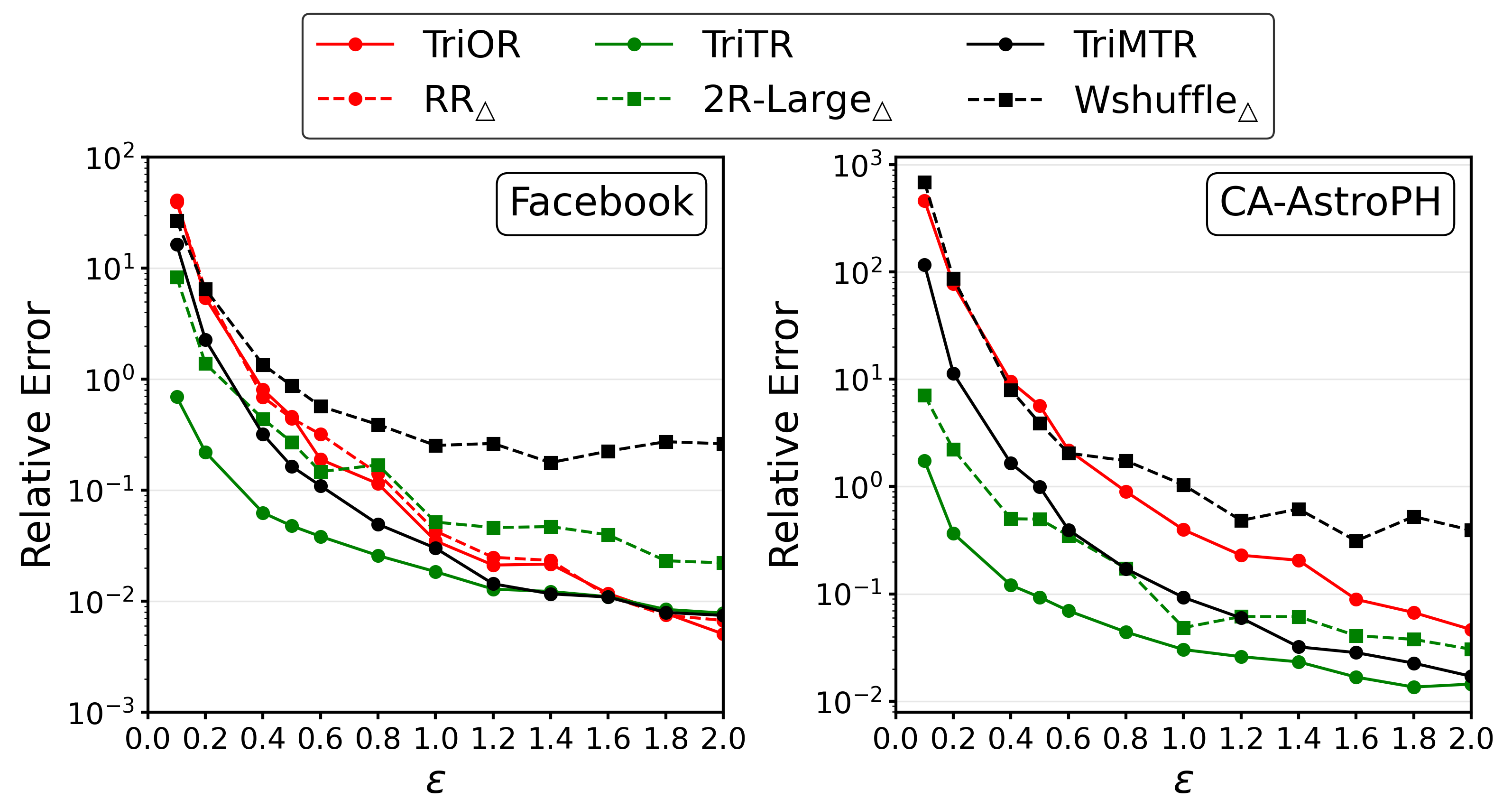
To RQ3, we replicate a subset of the algorithms from Table 2: , , and . These three are compared with our TriOR, TriTR, and TriMTR, respectively. The use of instead of is based on the findings in [24], which demonstrate that consistently outperforms in practical performance.


8.2 Experimental Results
Figures 6 provides answers to RQ1. A comparison between the RR and Laplace mechanisms shows that, under the same privacy budget, RR consistently achieves higher accuracy than the Laplace mechanism. This is consistent with the theory presented in the paper, as the variance of RR is approximately half that of the Laplace mechanism under the same privacy budget. Additionally, it is noticeable that the curves for RR and Laplace corresponding to TriOR, TriMTR, and TriTR diverge more as the privacy budget decreases. This is because their variances are inversely proportional to , , and , respectively. Furthermore, the accuracy of TriOR, TriMTR, and TriTR decreases as decreases, which is also due to the same reason. Since RR achieves higher accuracy and existing algorithms also use RR, all following data will use RR in GNAM.
Figures 7 provides answers to RQ2. A comparison between the red and green lines reveals minimal divergence, indicating that a slight reduction in has negligible impact on overall accuracy. Comparative analysis reveals a larger divergence in TriTR between the blue and green trajectories, whereas TriMTR and QuaTR exhibit marginal variations. This shows that GraphProjection is not the primary determinant of accuracy degradation. The most noticeable change occurs after the addition of second-round noise, where the relative error of the three two-round algorithms shows a more significant increase.
Figures 8 provides answers to RQ3. As demonstrated, all solid lines remain consistently below their dashed counterparts (except TriOR and ), which is perfectly consistent with the theoretical analysis presented in Section 7. The observed anomalies in TriOR and arise from the scaling operation applied to during the theoretical MSE derivation process. The triplet enumeration based required 63,033 s for 240 estimations on Facebook dataset (vs. TriOR’s 780 s). In CA-AstroPH, TriOR required 17, 955 s, while ’s prohibitive computational cost prevented its evaluation.
| (a) Facebook | ||||
|---|---|---|---|---|
| Algorithm | RE () | RE () | Time | |
| TriOR | s | 0 | ||
| TriTR | s | 124.97 MB | ||
| TriMTR | s | 31.58 KB | ||
| QuaTR | s | 124.97 MB | ||
| 2STAR | s | 0 | ||
| (b) CA-AstroPH | ||||
| Algorithm | RE () | RE () | Time | |
| TriOR | s | 0 | ||
| TriTR | s | 2.66 GB | ||
| TriMTR | s | 147.46 KB | ||
| QuaTR | s | 2.66 GB | ||
| 2STAR | s | 0 | ||
Figure 9 compares the 2-star counting algorithms. It can be observed that 2STAR achieves higher accuracy than . On CA-AstroPH, 2STAR exhibits a faster decreasing rate, which is due to its lower . This causes the term in its MSE to play a more significant role, resulting in a higher rate of change with respect to .
Tables 3 provides the accuracy, computation time and of our algorithms. The data is stored in float64 format. From the perspective of relative error, the four algorithms achieve high accuracy (RE < ). It can also be observed that the algorithm achieves higher accuracy on Facebook compared to CA-AstroPH. For TriOR, this is due to the increase in , as the actual number of triangles struggles to keep up with the growth of the term in MSE. As for the two-round algorithms, this is primarily because Facebook has larger .
9 Conclusion
This paper proposes TriOR, TriTR, TriMTR, and QuaTR algorithms based on the properties of noisy adjacency matrices. We implement edge LDP guarantees for the second round of two-round algorithms using a confidence interval-inspired mechanism, while designing the 2STAR algorithm for 2-star counting. Theoretical upper bounds on MSE are established for every algorithm. The experimental evaluation demonstrates that TriOR achieves an accuracy comparable to the existing one-round algorithm while reducing the time complexity to . Other proposed algorithms exhibit precision improvements over existing algorithms. All Algorithms maintain relative errors below 0.4 with reasonable privacy budgets .
In future work, we will integrate the noisy adjacency matrix with the graph convolutional neural network to enable model training while preserving users’ edge privacy.
References
- [1] Acharya, J., Sun, Z., and Zhang, H. Hadamard response: Estimating distributions privately, efficiently, and with little communication. In The 22nd International Conference on Artificial Intelligence and Statistics (2019), PMLR, pp. 1120–1129.
- [2] Aliakbarpour, M., Biswas, A. S., Gouleakis, T., Peebles, J., Rubinfeld, R., and Yodpinyanee, A. Sublinear-time algorithms for counting star subgraphs via edge sampling. Algorithmica 80 (2018), 668–697.
- [3] Avron, H. Counting triangles in large graphs using randomized matrix trace estimation. In Workshop on Large-scale Data Mining: Theory and Applications (2010), vol. 10, p. 9.
- [4] Balle, B., Bell, J., Gascón, A., and Nissim, K. The privacy blanket of the shuffle model. In Advances in Cryptology–CRYPTO 2019: 39th Annual International Cryptology Conference, Santa Barbara, CA, USA, August 18–22, 2019, Proceedings, Part II 39 (2019), Springer, pp. 638–667.
- [5] Bera, S. K., and Seshadhri, C. How the degeneracy helps for triangle counting in graph streams. In Proceedings of the 39th ACM SIGMOD-SIGACT-SIGAI Symposium on Principles of Database Systems (2020), pp. 457–467.
- [6] Bernau, D., Robl, J., Grassal, P. W., Schneider, S., and Kerschbaum, F. Comparing local and central differential privacy using membership inference attacks. In IFIP Annual Conference on Data and Applications Security and Privacy (2021), Springer, pp. 22–42.
- [7] Bi, M., Wang, Y., Cai, Z., and Tong, X. A privacy-preserving mechanism based on local differential privacy in edge computing. China Communications 17, 9 (2020), 50–65.
- [8] Björklund, A., Lokshtanov, D., Saurabh, S., and Zehavi, M. Approximate counting of k-paths: Deterministic and in polynomial space. In 46th International Colloquium on Automata, Languages, and Programming (ICALP 2019) (2019), Schloss Dagstuhl-Leibniz-Zentrum fuer Informatik.
- [9] Cheu, A., Smith, A., Ullman, J., Zeber, D., and Zhilyaev, M. Distributed differential privacy via shuffling. In Advances in Cryptology–EUROCRYPT 2019: 38th Annual International Conference on the Theory and Applications of Cryptographic Techniques, Darmstadt, Germany, May 19–23, 2019, Proceedings, Part I 38 (2019), Springer, pp. 375–403.
- [10] Chiba, N., and Nishizeki, T. Arboricity and subgraph listing algorithms. SIAM Journal on computing 14, 1 (1985), 210–223.
- [11] Coppersmith, D., and Winograd, S. Matrix multiplication via arithmetic progressions. In Proceedings of the nineteenth annual ACM symposium on Theory of computing (1987), pp. 1–6.
- [12] Dong, J., Roth, A., and Su, W. J. Gaussian differential privacy. Journal of the Royal Statistical Society: Series B (Statistical Methodology) 84, 1 (2022), 3–37.
- [13] Duan, R., Wu, H., and Zhou, R. Faster matrix multiplication via asymmetric hashing. In 2023 IEEE 64th Annual Symposium on Foundations of Computer Science (FOCS) (2023), IEEE, pp. 2129–2138.
- [14] Dwork, C. Differential privacy. In International colloquium on automata, languages, and programming (2006), Springer, pp. 1–12.
- [15] Dwork, C., McSherry, F., Nissim, K., and Smith, A. Calibrating noise to sensitivity in private data analysis. In Theory of Cryptography: Third Theory of Cryptography Conference, TCC 2006, New York, NY, USA, March 4-7, 2006. Proceedings 3 (2006), Springer, pp. 265–284.
- [16] Dwork, C., Roth, A., et al. The algorithmic foundations of differential privacy. Foundations and Trends® in Theoretical Computer Science 9, 3–4 (2014), 211–407.
- [17] Eden, T., Levi, A., Ron, D., and Seshadhri, C. Approximately counting triangles in sublinear time. SIAM Journal on Computing 46, 5 (2017), 1603–1646.
- [18] Eden, T., Liu, Q. C., Raskhodnikova, S., and Smith, A. Triangle counting with local edge differential privacy. arXiv preprint arXiv:2305.02263 (2023).
- [19] Erlingsson, Ú., Feldman, V., Mironov, I., Raghunathan, A., Talwar, K., and Thakurta, A. Amplification by shuffling: From local to central differential privacy via anonymity. In Proceedings of the Thirtieth Annual ACM-SIAM Symposium on Discrete Algorithms (2019), SIAM, pp. 2468–2479.
- [20] Feldman, V., McMillan, A., and Talwar, K. Hiding among the clones: A simple and nearly optimal analysis of privacy amplification by shuffling. In 2021 IEEE 62nd Annual Symposium on Foundations of Computer Science (FOCS) (2022), IEEE, pp. 954–964.
- [21] Gonen, M., Ron, D., and Shavitt, Y. Counting stars and other small subgraphs in sublinear-time. SIAM Journal on Discrete Mathematics 25, 3 (2011), 1365–1411.
- [22] Imola, J., Murakami, T., and Chaudhuri, K. Locally differentially private analysis of graph statistics. In 30th USENIX security symposium (USENIX Security 21) (2021), pp. 983–1000.
- [23] Imola, J., Murakami, T., and Chaudhuri, K. Communication-Efficient triangle counting under local differential privacy. In 31st USENIX security symposium (USENIX Security 22) (2022), pp. 537–554.
- [24] Imola, J., Murakami, T., and Chaudhuri, K. Differentially private triangle and 4-cycle counting in the shuffle model. In Proceedings of the 2022 ACM SIGSAC Conference on Computer and Communications Security (2022), pp. 1505–1519.
- [25] Jian, X., Wang, Y., and Chen, L. Publishing graphs under node differential privacy. IEEE Transactions on Knowledge and Data Engineering 35, 4 (2021), 4164–4177.
- [26] Kairouz, P., Bonawitz, K., and Ramage, D. Discrete distribution estimation under local privacy. In International Conference on Machine Learning (2016), PMLR, pp. 2436–2444.
- [27] Kallaugher, J., McGregor, A., Price, E., and Vorotnikova, S. The complexity of counting cycles in the adjacency list streaming model. In Proceedings of the 38th ACM SIGMOD-SIGACT-SIGAI Symposium on Principles of Database Systems (2019), pp. 119–133.
- [28] Kartun-Giles, A. P., and Kim, S. Counting -hop paths in the random connection model. IEEE Transactions on Wireless Communications 17, 5 (2018), 3201–3210.
- [29] Kasiviswanathan, S. P., Nissim, K., Raskhodnikova, S., and Smith, A. Analyzing graphs with node differential privacy. In Theory of Cryptography: 10th Theory of Cryptography Conference, TCC 2013, Tokyo, Japan, March 3-6, 2013. Proceedings (2013), Springer, pp. 457–476.
- [30] Kolountzakis, M. N., Miller, G. L., Peng, R., and Tsourakakis, C. E. Efficient triangle counting in large graphs via degree-based vertex partitioning. Internet Mathematics 8, 1-2 (2012), 161–185.
- [31] Le Gall, F. Powers of tensors and fast matrix multiplication. In Proceedings of the 39th international symposium on symbolic and algebraic computation (2014), pp. 296–303.
- [32] Leskovec, J., Kleinberg, J., and Faloutsos, C. Graph evolution: Densification and shrinking diameters. ACM transactions on Knowledge Discovery from Data (TKDD) 1, 1 (2007), 2–es.
- [33] Leskovec, J., and Krevl, A. SNAP Datasets: Stanford large network dataset collection. http://snap.stanford.edu/data, June 2014.
- [34] Leskovec, J., and Mcauley, J. Learning to discover social circles in ego networks. Advances in neural information processing systems 25 (2012).
- [35] Liu, Y., Zhao, S., Liu, Y., Zhao, D., Chen, H., and Li, C. Collecting triangle counts with edge relationship local differential privacy. In 2022 IEEE 38th International Conference on Data Engineering (ICDE) (2022), IEEE, pp. 2008–2020.
- [36] Manjunath, M., Mehlhorn, K., Panagiotou, K., and Sun, H. Approximate counting of cycles in streams. In Algorithms–ESA 2011: 19th Annual European Symposium, Saarbrücken, Germany, September 5-9, 2011. Proceedings 19 (2011), Springer, pp. 677–688.
- [37] McGregor, A., and Vorotnikova, S. Triangle and four cycle counting in the data stream model. In Proceedings of the 39th ACM SIGMOD-SIGACT-SIGAI Symposium on Principles of Database Systems (2020), pp. 445–456.
- [38] McSherry, F. D. Privacy integrated queries: an extensible platform for privacy-preserving data analysis. In Proceedings of the 2009 ACM SIGMOD International Conference on Management of data (2009), pp. 19–30.
- [39] Morris, C. The number of data breaches in 2021 has already surpassed last year’s total, 2021.
- [40] Murakami, T., and Kawamoto, Y. Utility-optimized local differential privacy mechanisms for distribution estimation. In 28th USENIX Security Symposium (USENIX Security 19) (2019), pp. 1877–1894.
- [41] Naseri, M., Hayes, J., and De Cristofaro, E. Local and central differential privacy for robustness and privacy in federated learning. arXiv preprint arXiv:2009.03561 (2020).
- [42] Nguyen, D., Halappanavar, M., Srinivasan, V., and Vullikanti, A. Faster approximate subgraph counts with privacy. Advances in Neural Information Processing Systems 36 (2024).
- [43] Nissim, K., Raskhodnikova, S., and Smith, A. Smooth sensitivity and sampling in private data analysis. In Proceedings of the thirty-ninth annual ACM symposium on Theory of computing (2007), pp. 75–84.
- [44] Ortmann, M., and Brandes, U. Triangle listing algorithms: Back from the diversion. In 2014 Proceedings of the Sixteenth Workshop on Algorithm Engineering and Experiments (ALENEX) (2014), SIAM, pp. 1–8.
- [45] Qin, Z., Yu, T., Yang, Y., Khalil, I., Xiao, X., and Ren, K. Generating synthetic decentralized social graphs with local differential privacy. In Proceedings of the 2017 ACM SIGSAC conference on computer and communications security (2017), pp. 425–438.
- [46] Raskhodnikova, S., and Smith, A. Differentially private analysis of graphs. Encyclopedia of Algorithms (2016).
- [47] Ribeiro, P., Paredes, P., Silva, M. E., Aparicio, D., and Silva, F. A survey on subgraph counting: concepts, algorithms, and applications to network motifs and graphlets. ACM Computing Surveys (CSUR) 54, 2 (2021), 1–36.
- [48] Satish, N., Sundaram, N., Patwary, M. M. A., Seo, J., Park, J., Hassaan, M. A., Sengupta, S., Yin, Z., and Dubey, P. Navigating the maze of graph analytics frameworks using massive graph datasets. In Proceedings of the 2014 ACM SIGMOD international conference on Management of data (2014), pp. 979–990.
- [49] Seshadhri, C., Pinar, A., and Kolda, T. G. Triadic measures on graphs: The power of wedge sampling. In Proceedings of the 2013 SIAM international conference on data mining (2013), SIAM, pp. 10–18.
- [50] Stothers, A. J. On the complexity of matrix multiplication.
- [51] Strassen, V. Gaussian elimination is not optimal. Numerische mathematik 13, 4 (1969), 354–356.
- [52] Tsourakakis, C. E., Kang, U., Miller, G. L., and Faloutsos, C. Doulion: counting triangles in massive graphs with a coin. In Proceedings of the 15th ACM SIGKDD international conference on Knowledge discovery and data mining (2009), pp. 837–846.
- [53] Wang, N., Zhang, J., Tan, K.-L., and Tung, A. K. On triangulation-based dense neighborhood graph discovery. Proceedings of the VLDB Endowment 4, 2 (2010), 58–68.
- [54] Wang, T., Blocki, J., Li, N., and Jha, S. Locally differentially private protocols for frequency estimation. In 26th USENIX Security Symposium (USENIX Security 17) (2017), pp. 729–745.
- [55] Wang, T., Mei, Y., Jia, W., Zheng, X., Wang, G., and Xie, M. Edge-based differential privacy computing for sensor–cloud systems. Journal of Parallel and Distributed computing 136 (2020), 75–85.
- [56] Wang, Y., Wu, X., and Hu, D. Using randomized response for differential privacy preserving data collection. In EDBT/ICDT Workshops (2016), vol. 1558, pp. 0090–6778.
- [57] Warner, S. L. Randomized response: A survey technique for eliminating evasive answer bias. Journal of the American Statistical Association 60, 309 (1965), 63–69.
- [58] Williams, V. V. Multiplying matrices faster than coppersmith-winograd. In Proceedings of the forty-fourth annual ACM symposium on Theory of computing (2012), pp. 887–898.
- [59] Yang, M., Guo, T., Zhu, T., Tjuawinata, I., Zhao, J., and Lam, K.-Y. Local differential privacy and its applications: A comprehensive survey. Computer Standards & Interfaces 89 (2024), 103827.
Appendix A Directed Graph Application
In the main text, we mentioned that our algorithm can be easily adapted to directed graphs. This is because, by simply removing the symmetry condition in the definition of the Noisy Adjacency Matrix, it can be seamlessly applied to directed graphs while still preserving all its properties.
Here, we provide the definition of the noisy adjacency matrix for directed graphs:
Definition 4 (Noisy adjacency matrix).
is the noisy adjacency matrix of directed graph , if satisfies:
;
.
where is the adjacency matrix of graph , is the number of nodes.
It still retains the properties stated in Theorem 1. Moreover, the subsequent algorithm design is largely similar to that for undirected graphs, with the only necessary adjustment being the consideration of directionality. Here, if we define triangles and quadrangles in directed graphs as 3/4-step loops without traversing the same edge more than once, the corresponding algorithms are as follows:
Among these changes, there are only three modifications: (1) the coefficient by which each algorithm divides at the end is adjusted to account for the single directionality of edges in directed graphs, as opposed to the bidirectional nature in undirected graphs; (2) in the quadrangle algorithm, there is no need to subtract 1 in line 5, as the directed nature of the edges prevents traversal back along the original path; and (3) in TriTR and QuaTR, when calculating , the noise relationship added changes from to .
Furthermore, although their variances do not match the specific expressions in undirected graphs, they still satisfy the Variance in Matrix Form when coefficients are ignored. The proofs for directed graphs are not elaborated in detail here, as the proof methodology closely resembles that used for undirected graphs.
Appendix B Weighted Graph Application
If the original adjacency matrix , it still retains the properties stated in Theorem 1, as the proof of Theorem 1 does not require to belong to . When dealing with weighted graphs, GNAM can utilize the Laplace mechanism for edge-LDP.
Appendix C Estimate Three Subgraphs in Two Rounds
| Dataset | TriMTR | QuaTR | 2STAR |
|---|---|---|---|
| 0.0301 | 0.1108 | 0.0052 | |
| CA-AstroPH | 0.0926 | 0.3531 | 0.0322 |
Table 4 shows the estimation performance for three subgraphs obtained by two-round query. We allocated to GraphProjection, to GNAM, to the second round of TriMTR, and to the second round of QuaTR. Thus, a total privacy budget of suffices to estimate all three subgraph counts while achieving the accuracy shown in the table.
Appendix D Second Round Risk without Randomizer
At the beginning of Chapter 6, we mentioned the necessity of addressing the issue of adding noise in the second round, as directly uploading is not feasible. Uploading directly would not only fail to provide -edge LDP in the second round but also expose to the following attack risks:
If the DP mechanism employed in GNAM is a continuous noise mechanism, such as the Laplace Mechanism or Gaussian Mechanism. Because the probability of the continuous random variable taking any specific value is zero, this characteristic enables the following potential attack strategy:
Assume adversary can obtain the noisy adjacency matrix . The adversary can enumerate node ’s possible neighbor list: . Denote the true neighbor list of user as . If a certain satisfies: For TriTR, ; For TriMTR, ; For QuaTR, . Then the adversary can determine that this is the correct neighbor list () of .
Appendix E Proof of Statements
E.1 Proof of Theorem 1
Given that the noisy adjacency matrix satisfies all the conditions of Definition 7, we can view from an alternative perspective: , where is the adjacency matrix of the original graph, and is a noise matrix that satisfies the following properties:
First properity.
.
For each :
Focusing on the second item:
The third item is similar to the second item. Then the forth item, since , and are independent. Therefore, we have:
Therefore, For each , .
Second peoperity.
.
For each :
The expected value of each subsequent term is zero except for the first term, .
For the second, third, and fourth terms, each summation contains only a single . Since , the expectation of these terms is also zero.
For the fifth, sixth, and seventh terms, each summation contains two terms and . Given and , if these terms are independent, their product has an expectation of zero. If they are not independent, or , there exist or , because for any , we have .
Therefore, the expectation of the fifth, sixth, and seventh terms is zero.
For the eighth term, each summation includes . If these three terms are independent, the expectation of their product is the product of their expectations, which equals zero. If at least two among , , and are not independent, then at least one pair among , , and must be equal. Then for any , , which consequently ensures that the product of them is zero. Therefore, in all cases, the expectation of the eighth term is zero. Then for each , .
E.2 Proof of Theorem 2
In the adjacency list of node , indicates that node can reach node in one step, while 0 indicates that it cannot. Thus, for any two adjacent adjacency lists and , they differ by at most one bit, . According to the Laplace mechanism theorem as guaranteed by [15], we have:
The local randomizer satisfies: for any two neighboring lists that differ by one bit and any ,
Thus, uploading can provide -edge LDP.
Each node only uploads the connection information with nodes that have a smaller index. This approach is taken to avoid the scenario where the information of the same edge is uploaded by both of its endpoints. According to the composition theorem [15], if an adversary gains access to information uploaded by both of them, it would only guarantee -edge differential privacy [43].
E.3 Proof of Proposition 3
If , then . If , then takes . Given the original true value is 1, we have the expected value . Given the original true value is 0, we have the expected value .
E.4 Proof of Theorem 3
Given that GNAM provides -edge LDP, and based on the immunity to post-processing [14], it follows that TriTR also provides -edge LDP.
E.5 Lemma 1
To facilitate subsequent proofs, let us get Lemma 1.
Lemma 1.
Let be a sequence of mutually independent random variables, and for each , . Then, for two finite integer sequences and , and their corresponding exponent sequences , satisfies:
And there exists a number , , and the corresponding exponent for that number is , it holds that:
Proof.
The expectation holds because there exists an , and the exponent of is 1. Because the independence among , can be factored out. Let denote the remaining product. Then we have:
E.6 Proof of Theorem 4
In the proof that follows, we continue to use the notation in Theorem 1, denoting .
The proof of unbiasedness follows easily from the second clause of Theorem 3:
Then the MSE:
.
On the diagnal:
Therefore:
According to Lemma 1, the variance of the aforementioned expression is equal to the sum of the variances of its individual components:
Next, the overall variance can be calculated by determining the variance of these four components. The first:
This is a constant, equal to , and its variance is 0.
The second item:
From the perspective of the graph, means that there exist a path starting from and passing through to in the actual graph. If this path exists, then will be added to this term. So will be added times. Since this is in an undirected graph, will also be added times, and , therefore:
Given that , we have:
Next, we analyze the third term:
If there exists an undirected edge in the graph, then will be added into the third term. Let if the proposition holds true, and otherwise. In addition, beacuse , therefore:
According to Lemma 1, and . Therefore:
The fourth term:
Since in an undirected graph, , , thus:
Based on Lemma 1, and , we get:
According to all the above equations, we get:
Even if each node has edges, there can be at most paths of the form in the graph. Each . Given a fixed number of paths like , concentrating all the paths on , each , can maximize to . In undirected graph, , and . Therefore:
Therefore,
E.7 Proof of Theorem 5
According to Theorem 3, GNAM provides -edge LDP, and since the second randomizer provides -edge LDP, by the composition theorem, the entire TriTR provides -edge LDP.
E.8 Proof of Theorem 6
Let us denote , where follows the same property as in Theorem 1. For each :
where is the number of triangles in which user is involved. Therefore:
The first item . For the second item, because , , we get:
In the proof of Theorem 4, we get:
Therefore:
Finally we get:
In the proof of Theorem 6, we have , therefore:
E.9 Proof of Theorem 7
Since GNAM provides an -edge LDP and the second round’s second randomizer provides -edge LDP, therefore, according to the composition theorem, TriMTR provides -edge LDP.
E.10 Proof of Theorem 8
Align with Theorem 1, . For each :
Therefore:
In the proof of Theorem 4, we get:
Therefore:
In the proof of Theorem 6, we have , , therefore:
E.11 Proof of Theorem 9
Since GNAM provides an -edge LDP and the second randomizer provides -edge LDP, therefore, according to the composition theorem, QuaMTR provides -edge LDP.
E.12 Proof of Theorem 10
Align with Theorem 1, . For each :
It should be noted that the physical meaning of is the number of ways node can return to itself after 4 steps. From the perspective of taking four steps, encompasses two scenarios: one is , which corresponds to the case where the same edge is traversed four times, specifically when ; the other scenario is , which involves traversing one edge twice and then another edge twice, specifically when . Therefore,
Here, represents the number of quadrangles that node is part of. This is because subtracting the two scenarios where the path does not involve four distinct nodes from all possible four-step paths leaves us with paths that traverse a quadrangle. Since each quadrangle is traversed in both directions, the count is twice that of . Therefore:
Then focus on the MSE (equals to Variance) part:
According to Lemma 1, we get:
The first item:
Let represent the number of ways to reach node from node in exactly three steps, i.e. .
Similarly to Theorem 6, based on Lemma 1 and the symmetry of and , we have the following:
The second item:
Let’s make some changes to the above expression.
From a graph perspective, represents the sum of the product of the adjacency relationships’ noise between node and node with the remaining nodes. Therefore, for different pairs of nodes and , and satisfy the conditions of Lemma 1. Hence, we have:
Then based on Lemma 1, we get:
Therefore:
In the given graph, each edge (denoted as ) represents the product of the degrees of its two vertices, which physically signifies the number of that have this edge as the middle edge. Taking all the edges in the graph, we can obtain the total number of such as follows:
The equation holds as an equality if and only if every node in the graph has edges.
Due to the maximum value of each being only , this situation occurs when every neighbor of node is connected to every neighbor of node . Therefore, we have . To maximize , we can set each . As mentioned above, , and therefore there can be at most instances of . At this point, reaches its maximum value of .
Therefore, .
E.13 Proof of Theorem 11
Let us first address Algorithm 7.
Denote neighbor adjacency list of , which is derived by either adding or removing a single neighbor from the original list of , let denote the index of the newly added neighbor. The resulting change in can be expressed as . Assuming that the newly added neighbor is connected by edges to all existing neighbors of user , the resulting increment in attains its maximum value. By the Central Limit Theorem:
The upper and lower quantiles are given by:
After Graph Projection on graph G, for any vertex , we have . Therefore, the absolute values of the upper and lower quantiles are less than:
Therefore:
The change in resulting from removing a neighbor from the original neighbor list of is less significant than the maximum change induced by adding a neighbor. Therefore, we focus solely on analyzing the impact of adding a neighbor on . By the same reasoning, the subsequent proofs will also restrict their discussion to the scenario of adding an edge to the adjacency list, as the case for removing an edge follows a similar logic.
Then deal with the Algorithm 8.
According to Lemma 1, we get:
Since for different , the terms are mutually independent, and their variances differ by at most , it follows from the Central Limit Theorem for independent but non-identically distributed random variables that:
Its upper and lower quantiles are given by:
Similarly, their absolute values are both less than:
Set for user , we have:
Then deal with the Algorithm 9. Readers may have noticed that calculating does not require determining its exact distribution. Instead, one can use looser bounds on the expectation and variance of the distribution, which ensures that the determined satisfies the two probability inequalities.
Any element in satisfies:
If a neighbor is added, the change in can be expressed as:. Assuming that each is equal to , and the variance of each is , the approximate distribution of can be described as follows:
According to Lemma 1 and the properties of the sum of multivariate normal distributions, even though the are not independent, we still obtain: the approximate distribution of is:
Therefore, set as:
satisfies:
E.14 Proof of Theorem 12
We proof the privacy guarantee firstly. If a user adds a neighbor , in line 2 of Algorithm 7, the maximum increase to would be . In line 2, the impact on is constrained to the range by the clamp function. Consequently, the maximum change to caused by adding a node is also . Therefore, according to the Laplace mechanism, adding noise ensures -edge LDP.
The multiplication by 2 at the end serves to ensure that the expected value of the final remains , thereby allowing it to be seamlessly integrated into Algorithm 3.
The composition theorem to be applied here is Proposition 1, where is derived from the output () of the GraphProjection function. In GraphProjection, -edge LDP is provided, in GNAM, -edge LDP is provided, and in Algorithm 7, -edge LDP is provided. Thus, according to Proposition 1, the overall system provides -edge LDP.
The total MSE can be divided into four parts. The first part is the error introduced by GraphProjection; the second part is that in the second round, Less than proportion of the data is clamped. The parameters affecting these two parts include , , and . Setting and to a larger value can reduce the number of edges removed. By setting to a smaller value, the amount of data that is clamped can be minimized. These two parts have a relatively small impact on the final MSE.
The main part of the MSE comes from the third and fourth parts. The third part is the error inside the , and the fourth part is the error introduced by the newly added Lap() in the second round. In Theorem 8, we have already obtained the MSE of the third part. Therefore, we focus on the fourth part.
Because the Laplace noise added in the second round for each node is not only independent of the part but also independent among the Laplace noises themselves, the variance of this part can be calculated as the sum of the variances of each individual Laplace noise.
Let the Laplace noise added in the second round by node be denoted as . For the sake of simplicity in the formula, let’s denote as . Once is determined, is a constant and will not be too large. For example, when is taken as , .
In the previous analysis, if using RR or Laplace mechanism, we have , and we have , therefore:
Therefore:
Combining this with Theorem 8, and , we get:
E.15 Proof of Theorem 13
We proof the privacy guarantee firstly. In essence, during the second round, user is presented with a sequence of data , from which selects numbers to sum and upload. The privacy to be protected here lies in the specific choice of numbers selected by . After applying the clamp function, the range of these numbers is effectively constrained to . If user gains or loses a neighbor, it essentially means adding or removing one number from this sequence. Since the impact of such a change on is bounded by , the mechanism ensures -edge LDP.
Following a reasoning similar to the proof of Theorem 12, and by applying Proposition 1, the overall system provides -edge LDP.
Then the total MSE.
Because the value of after clamping will not exceed , the second round will provide -edge LDP. By combining this with the composition theorem, TriMTR will provide a total of -edge LDP.
Using the same notation as in Theorem 14, let be the Laplace noise added to node in the second round, and . We have:
In the previous analysis, if using RR or Laplace mechanism, we have , and we have , therefore:
Therefore:
Combining this with Theorem 8, and , we get:
E.16 Proof of Theorem 14
The method to prove the provision of -edge LDP is similar to the methods used in Theorem 2, so we will not elaborate further here. Next, we will bound its MSE.
Using the same notation as in Theorem 14, let be the Laplace noise added to node in the second round, and . We have:
In the previous analysis, if using RR or Laplace mechanism, we have , and we have , therefore:
Therefore:
Combining this with Theorem 8, and , we get:
E.17 Proof of Theorem 15
Given the assumption that the clustering coefficient of a graph remains constant, the number of triangles in the graph is proportional to the number of 2-stars in the graph. This relationship can be denoted as .
Considering a 2-star to be composed of a central node and its two incident edges, the total number of 2-stars in the graph can be calculated by the following formula:
Therefore, .
Here, we focus specifically on the impact of the privacy budget and the structure of the graph (number of nodes and the degree values ) on convergence. We primarily consider the order of magnitude and treat other terms as constant coefficients. Therefore, we get .
First, we address TriTR, whose more precise expression for MSE is:
Because , Therefore:
Therefore:
According to Jensen’s inequality, we have:
Then the RE:
Because , with equality if and only if for any . Therefore:
Next, we address TriMTR. Because , the more precise expression for the MSE of TriTR is:
Using a similar scaling method as TriTR, we obtain:
Therefore, the Relative Err:
E.18 Proof of Theorem 16
Proof. Given the true number:
Let , then , , , , the first property:
Second property:
Treating as a constant, we obtain:
Thus:
