跳到论文正文
W Papers独立论文阅读器 arXiv:2507.02459 论文正文 计算阅读时间 · 0%
引用这篇论文根据当前论文元数据生成,正式投稿前建议核对。


A modified Crank-Nicolson scheme for the Vlasov-Poisson system with a strong external magnetic field

Francis Filbet Institut de Mathématiques de Toulouse, Université Paul Sabatier, Toulouse, France francis.filbet@math.univ-toulouse.fr ,  L. Miguel Rodrigues Univ Rennes, CNRS, IRMAR - UMR 6625, F-35000 Rennes, France luis-miguel.rodrigues@univ-rennes.fr  and  Kim Han Trinh Univ Rennes, CNRS, IRMAR - UMR 6625, F-35000 Rennes, France kim-han.trinh@univ-rennes.fr
Abstract.

We propose and study a Particle-In-Cell (PIC) method utilizing Crank-Nicolson time discretization for the Vlasov-Poisson system with a strong, inhomogeneous external magnetic field with fixed direction. Our focus is on particle dynamics in the plane orthogonal to the magnetic field – commonly referred to as the poloidal plane. In this regime, traditional explicit schemes are constrained by stability conditions linked to the small Larmor radius and plasma frequency [21]. To avoid this limitation, our approach is based on numerical schemes [9, 10, 12], providing a consistent PIC discretization of the guiding-center system taking into account variations of the magnetic field. We carry out some theoretical proofs and perform several numerical experiments to validate the method demonstrating its robustness and accuracy.

Key words and phrases:
Vlasov-Poisson systems; Strong magnetic field; Particle methods.
2010 Mathematics Subject Classification:
Primary: 65M75 Secondary: 82D10 76X05 35Q83
Research of L.M.R. was partially supported by the ANR Project HEAD ANR-24-CE40-3260 and the Institut Universitaire de France.
Research of K.H.T. was partially supported by the Institut Universitaire de France.

1. Introduction

This paper focuses on plasma confinement in the presence of a strong, spatially varying external magnetic field, where charged particles evolve under the influence of both electrostatic forces and intense magnetic confinement. Such configurations are characteristic of tokamak plasmas [1, 19], where the magnetic field plays a crucial role in containing particles within the core of the device. Kinetic models, which provide a mesoscopic description of charged particle dynamics, are highly accurate and essential tools for investigating the behavior of thermonuclear fusion plasmas.
We assume that collective effects dominate, and the plasma is modeled entirely through transport equations. The primary unknown is the particle number density f≡f​(t,𝐱,𝐯)f\equiv f(t,{\mathbf{x}},{\mathbf{v}}), which depends on time t≥0t\geq 0, position 𝐱∈Ω⊂ℝd{\mathbf{x}}\in\Omega\subset{\mathbb{R}}^{d}, and velocity 𝐯∈ℝd{\mathbf{v}}\in{\mathbb{R}}^{d}, with d≥2d\geq 2. Its behaviour is given by the Vlasov equation,

(1.1) ∂f∂t+𝐯⋅∇𝐱f+𝐅​(t,𝐱,𝐯)⋅∇𝐯f= 0,\frac{\partial f}{\partial t}\,+\,{\mathbf{v}}\cdot\nabla_{\mathbf{x}}f\,+\,\mathbf{F}(t,{\mathbf{x}},{\mathbf{v}})\cdot\nabla_{\mathbf{v}}f\,=\,0,

where the force field F​(t,𝐱,𝐯)F(t,{\mathbf{x}},{\mathbf{v}}) is coupled with the distribution function ff giving a nonlinear system.

Here, we consider the two-dimensional case where the magnetic field acts in the vertical direction and only depends on 𝐱=(x1,x2)∈ℝ2{\mathbf{x}}=(x_{1},x_{2})\in{\mathbb{R}}^{2}, that is,

𝐁​(𝐱)=1ε​(00b​(𝐱)),{\mathbf{B}}({\mathbf{x}})\,\,=\,\,\frac{1}{\varepsilon}\,\left(\begin{array}[]{l}0\\ 0\\ b({\mathbf{x}})\end{array}\right)\,,

where the function bb describes the variations of the amplitude with b∈W1,∞​(ℝ2)b\in W^{1,\infty}(\mathbb{R}^{2}) and

(1.2) b​(𝐱)≥b0>0.b({\mathbf{x}})\geq b_{0}>0\,.

The number ε>0\varepsilon>0 is a small parameter related to the ratio between the reciprocal Larmor frequency and the advection time scale (see [8, 18, 17] and the references therein for more details on scalings).

We will focus on the long-time behavior of positive ions in the orthogonal plane to the external magnetic field. Therefore, the distribution function fεf_{\varepsilon} is a solution to the Vlasov equation coupled with the Poisson equation for the electrical potential ϕε\phi_{\varepsilon} generated by the motion of these charged particles, that is,

(1.3) {ε​∂fε∂t+𝐯⋅∇𝐱fε+(𝐄ε​(t,𝐱)−b​(𝐱)​𝐯⟂ε)⋅∇𝐯fε= 0,𝐄ε=−∇𝐱ϕε,−Δ𝐱​ϕε=ρε,\displaystyle\begin{dcases}\varepsilon\dfrac{\partial f_{\varepsilon}}{\partial t}\,+\,\mathbf{v}\cdot\nabla_{\mathbf{x}}f_{\varepsilon}\,+\,\left(\mathbf{E}_{\varepsilon}(t,\mathbf{x})-b(\mathbf{x})\,\dfrac{\mathbf{v}^{\perp}}{\varepsilon}\right)\cdot\nabla_{\mathbf{v}}f_{\varepsilon}\,=\,0\,,\\ \mathbf{E}_{\varepsilon}\,=\,-\nabla_{\mathbf{x}}\phi_{\varepsilon}\,,\qquad-\Delta_{\mathbf{x}}\phi_{\varepsilon}\,=\,\rho_{\varepsilon}\,,\end{dcases}

where 𝐯⟂=(−v2,v1)∈ℝ2{\mathbf{v}}^{\perp}\,=\,(-v_{2},v_{1})\in{\mathbb{R}}^{2} and the density ρε\rho_{\varepsilon} is given by

ρε​(t,𝐱):=∫ℝ2fε​(t,𝐱,𝐯)​d𝐯.\rho_{\varepsilon}(t,\mathbf{x})\,:=\,\displaystyle\int_{\mathbb{R}^{2}}f_{\varepsilon}(t,{\mathbf{x}},{\mathbf{v}})\,\mathrm{d}{\mathbf{v}}\,.

Here we aim to construct numerical approximations for the Vlasov-Poisson system (1.3) using particle methods (see [2]), which involve in approximating the distribution function by a finite number of macro-particles. The trajectories of these particles are determined from the characteristic curves associated to the Vlasov equation

(1.4) {ε​d​𝐱εd​t=𝐯ε,ε​d​𝐯εd​t=𝐄ε​(t,𝐱ε)−b​(𝐱ε)​𝐯ε⟂ε,𝐱ε​(0)=𝐱ε0,𝐯ε​(0)=𝐯ε0,\displaystyle\begin{dcases}\varepsilon\dfrac{\mathrm{d}\mathbf{x}_{\varepsilon}}{\mathrm{d}t}=\mathbf{v}_{\varepsilon}\,,\\[8.00003pt] \varepsilon\dfrac{\mathrm{d}\mathbf{v}_{\varepsilon}}{\mathrm{d}t}=\mathbf{E}_{\varepsilon}(t,\mathbf{x}_{\varepsilon})-b(\mathbf{x}_{\varepsilon})\dfrac{\mathbf{v}_{\varepsilon}^{\perp}}{\varepsilon}\,,\\[8.00003pt] \mathbf{x}_{\varepsilon}(0)=\mathbf{x}_{\varepsilon}^{0}\,,\qquad\mathbf{v}_{\varepsilon}(0)=\mathbf{v}_{\varepsilon}^{0}\,,\end{dcases}

then we use the conservation of fεf_{\varepsilon} along the characteristic curves, that is,

fε​(t,𝐱ε​(t),𝐯ε​(t))=fε​(t0,𝐱ε0,𝐯ε0).\displaystyle f_{\varepsilon}(t,\mathbf{x}_{\varepsilon}(t),\mathbf{v}_{\varepsilon}(t))\,=\,f_{\varepsilon}(t^{0},\mathbf{x}^{0}_{\varepsilon},\mathbf{v}^{0}_{\varepsilon})\,.

In particular, we will focus on the construction of numerical schemes for the ODE system (1.4), where the time step Δ​t\Delta t is arbitrary and free from any stability constraint. Following the work of Filbet and Rodrigues [10, 11, 12], the ODE system can be decomposed into fast dynamics, driven by the fast variable 𝐯ε{\mathbf{v}}_{\varepsilon}, and slow dynamics, governed by the variables (𝐱ε,eε)({\mathbf{x}}_{\varepsilon},e_{\varepsilon}), where eε=12​|𝐯ε|2e_{\varepsilon}=\frac{1}{2}|{\mathbf{v}}_{\varepsilon}|^{2}. This decomposition allows the design of a class of numerical schemes that precisely capture slow-scale variables, while faster scales are correctly filtered. More precisely, when the intensity of the magnetic field is sufficiently large, i.e. when ε≪1\varepsilon\ll 1, the scheme provides a consistent approximation to the asymptotic model [10].

1.1. Formal asymptotic behavior for a given electromagnetic field

Before describing a numerical scheme for the nonlinear Vlasov-Poisson system (1.3), we first briefly expound on what may be expected from the continuous model with a given electric field in the limit ε→0\varepsilon\to 0. For this purpose, we consider a function ϕ∈W3,∞\phi\in W^{3,\infty} such that, for all 𝐱∈ℝ2\mathbf{x}\in\mathbb{R}^{2}, 𝐄​(𝐱)=−∇𝐱ϕ​(𝐱)\mathbf{E}(\mathbf{x})=-\nabla_{\mathbf{x}}\phi(\mathbf{x}) and observe that the system (1.4) has an Hamiltonian structure associated with the total energy ℰε​(t)\mathcal{E}_{\varepsilon}(t),

(1.5) ℰε​(t)=‖𝐯ε​(t)‖22+ϕ​(𝐱ε​(t)),t≥0,\displaystyle\mathcal{E}_{\varepsilon}(t)=\dfrac{\|\mathbf{v}_{\varepsilon}(t)\|^{2}}{2}+\phi(\mathbf{x}_{\varepsilon}(t)),\qquad t\geq 0\,,

which is an invariant of the system. Therefore, to study the limit ε→0\varepsilon\rightarrow 0, we first define the kinetic energy as a slow scale variable

eε​(t):=12​‖𝐯ε​(t)‖2,e_{\varepsilon}(t)\,:=\,\frac{1}{2}\|\mathbf{v}_{\varepsilon}(t)\|^{2}\,,

leading to the study of the augmented system

(1.6) {d​𝐱εd​t=𝐯εε,d​eεd​t=1ε​𝐄​(𝐱ε)⋅𝐯ε,\displaystyle\begin{dcases}\dfrac{\mathrm{d}\mathbf{x}_{\varepsilon}}{\mathrm{d}t}\,=\,\frac{\mathbf{v}_{\varepsilon}}{\varepsilon}\,,\\[8.99994pt] \dfrac{\mathrm{d}e_{\varepsilon}}{\mathrm{d}t}\;=\,\frac{1}{\varepsilon}\,\mathbf{E}(\mathbf{x}_{\varepsilon})\cdot\mathbf{v}_{\varepsilon}\,,\end{dcases}

still coupled with the equation on 𝐯ε{\mathbf{v}}_{\varepsilon}

(1.7) ε​d​𝐯εd​t=𝐄​(𝐱ε)−b​(𝐱ε)​𝐯ε⟂ε,\varepsilon\dfrac{\mathrm{d}\mathbf{v}_{\varepsilon}}{\mathrm{d}t}\,=\,\mathbf{E}(\mathbf{x}_{\varepsilon})\,-\,b(\mathbf{x}_{\varepsilon})\,\dfrac{\mathbf{v}_{\varepsilon}^{\perp}}{\varepsilon}\,,

which describes the fastest scale. Of course the second equation of (1.6) is a consequence of (1.7) but it retains only its slower part.

Following [11], one may prove that 𝐱ε​(t)→𝐲​(t)\mathbf{x}_{\varepsilon}(t)\rightarrow\mathbf{y}(t) and eε​(t)→g​(t)e_{\varepsilon}(t)\rightarrow g(t), as ε→0\varepsilon\rightarrow 0 where (𝐲,g)(\mathbf{y},g) is solution to the so-called guiding center system,

(1.8) {d​𝐲d​t=−𝐄⟂b​(𝐲)+g​∇𝐲⟂bb2​(𝐲),d​gd​t=g​𝐄⋅∇𝐲⟂bb2​(𝐲).\displaystyle\begin{dcases}\dfrac{\mathrm{d}\mathbf{y}}{\mathrm{d}t}\,=\,-\dfrac{\mathbf{E}^{\perp}}{b}(\mathbf{y})\,+\,g\,\dfrac{\nabla_{\mathbf{y}}^{\perp}b}{b^{2}}(\mathbf{y})\,,\\[8.99994pt] \dfrac{\mathrm{d}g}{\mathrm{d}t}\,=\,g\,\mathbf{E}\cdot\dfrac{\nabla_{\mathbf{y}}^{\perp}b}{b^{2}}(\mathbf{y})\,.\end{dcases}

For the convenience of the reader we provide in Appendix A the main formal computations leading to (1.8).

Furthermore, we may identify the limit for the total energy ℰε​(t)\mathcal{E}_{\varepsilon}(t), as ε→0\varepsilon\rightarrow 0, this quantity converging to

ℰg​c​(t):=g​(t)+ϕ​(𝐲​(t)),\displaystyle\mathcal{E}_{gc}(t)\,:=\,g(t)\,+\,\phi(\mathbf{y}(t))\,,

which is indeed an invariant of the guiding center model (1.8),

(1.9) d​ℰg​cd​t=d​gd​t+∇𝐲ϕ​(𝐲)⋅d​𝐲d​t=g​𝐄⋅∇𝐲⟂bb2​(𝐲)−g​𝐄⋅∇𝐲⟂bb2​(𝐲)= 0.\displaystyle\dfrac{\mathrm{d}\mathcal{E}_{gc}}{\mathrm{d}t}\,=\,\dfrac{\mathrm{d}g}{\mathrm{d}t}\,+\,\nabla_{\mathbf{y}}\phi(\mathbf{y})\cdot\dfrac{\mathrm{d}\mathbf{y}}{\mathrm{d}t}\,=\,g\,\mathbf{E}\cdot\dfrac{\nabla_{\mathbf{y}}^{\perp}b}{b^{2}}(\mathbf{y})\,-\,g\,\mathbf{E}\cdot\dfrac{\nabla_{\mathbf{y}}^{\perp}b}{b^{2}}(\mathbf{y})\,=\,0\,.

Furthermore, we may define the magnetic moment as

μg​c​(t)=gb​(𝐲),\mu_{gc}(t)\,=\,\dfrac{g}{b(\mathbf{y})}\,,

which is an invariant for the guiding center system (1.8) without counterpart for the original (1.4), thus called an adiabatic invariant for (1.8). Indeed, we have

(1.10) d​μg​cd​t=dd​t​(gb​(𝐲))=g​𝐄⋅∇𝐲⟂bb3​(𝐲)−g​∇𝐲bb2​(𝐲)⋅(−𝐄⟂b​(𝐲)+g​∇𝐲⟂bb2​(𝐲))= 0.\displaystyle\dfrac{\mathrm{d}\mu_{gc}}{\mathrm{d}t}\,=\,\dfrac{\mathrm{d}}{\mathrm{d}t}\left(\dfrac{g}{b(\mathbf{y})}\right)\,=\,g\,\mathbf{E}\cdot\dfrac{\nabla_{\mathbf{y}}^{\perp}b}{b^{3}}(\mathbf{y})\,-\,g\dfrac{\nabla_{\mathbf{y}}b}{b^{2}}(\mathbf{y})\cdot\left(-\dfrac{\mathbf{E}^{\perp}}{b}(\mathbf{y})+g\dfrac{\nabla_{\mathbf{y}}^{\perp}b}{b^{2}}(\mathbf{y})\right)\,=\,0\,.

Reproducing these properties at the discrete level is a target when designing a scheme for (1.4) preserving asymptotics when ε\varepsilon tends to zero.

1.2. Formal asymptotic limit of the Vlasov-Poisson system

We come back to the Vlasov-Poisson system (1.3). Here one cannot anymore remain completely at the characteristic level (1.4). Moreover whereas arguments of the previous subsection could be turned into sound analytic arguments (by slight variations on [11]), to the best of our knowledge the present situation does not fall directly into the range of the actually available analysis of gyro-kinetic limits. We refer the reader to the introductions of [11, 24] and references therein for a representative sample of such analytic techniques.

Nevertheless the known results and the previous subsection strongly suggests for (fε,𝐄ε)(f^{\varepsilon},{\mathbf{E}}^{\varepsilon}) solving the Vlasov-Poisson system (1.3) that in the limit ε→0\varepsilon\rightarrow 0, the electric field 𝐄ε{\mathbf{E}}^{\varepsilon} and the following velocity-averaged version of F¯ε\bar{F}^{\varepsilon}

F¯ε:(t,𝐱,e)↦12​π​∫02​πfε​(t,𝐱,2​e​(cos⁡(θ),sin⁡(θ)))​dθ\bar{F}^{\varepsilon}\,:\,(t,{\mathbf{x}},e)\mapsto\frac{1}{2\pi}\int_{0}^{2\pi}f^{\varepsilon}(t,{\mathbf{x}},\sqrt{2e}(\cos(\theta),\sin(\theta)))\,\mathrm{d}\theta

converge to some 𝐄:(t,𝐲)↦𝐄​(t,𝐲){\mathbf{E}}:(t,\mathbf{y})\mapsto{\mathbf{E}}(t,\mathbf{y}) and some111We use distinct notation of variables for limiting functions to be consistent with asymptotic analysis at the characteristic level. This is of course completely immaterial. f:(t,𝐲,g)↦f​(t,𝐲,g)f:(t,\mathbf{y},g)\mapsto f(t,\mathbf{y},g) solving the following system consisting in a transport equation supplemented with a Poisson equation,

(1.11) {∂f∂t+𝐔⋅∇𝐲f+ug​∂f∂g= 0,−Δ𝐲​ϕ=ρ,ρ=2​π​∫ℝ+f​dg,\left\{\begin{array}[]{l}\displaystyle\frac{\partial f}{\partial t}\,+\,\mathbf{U}\cdot\nabla_{\mathbf{y}}f\,+\,u_{g}\frac{\partial f}{\partial g}\,=\,0,\\ \\ \displaystyle-\Delta_{\mathbf{y}}\phi\,=\,\rho\,,\quad\rho=2\pi\,\int_{{\mathbb{R}}^{+}}f\,\mathrm{d}g,\end{array}\right.

where the velocity field is given by

𝐔​(t,𝐲,g)=𝐅​(t,𝐲)+g​∇𝐲⟂bb2​(t,𝐲),ug=−div𝐲​(𝐅)​(t,𝐲)​g,{\bf U}(t,\mathbf{y},g)\,=\,{\mathbf{F}}(t,\mathbf{y})\,+\,g\,\frac{\nabla_{\mathbf{y}}^{\perp}b}{b^{2}}(t,\mathbf{y})\,,\qquad u_{g}=-{\rm div}_{\mathbf{y}}({\mathbf{F}})(t,\mathbf{y})\,g\,,

with 𝐄=−∇𝐲ϕ{\mathbf{E}}=-\nabla_{\mathbf{y}}\phi, 𝐅=−𝐄⟂/b{\mathbf{F}}=-{\mathbf{E}}^{\perp}/b. We remind the reader that 𝐔{\mathbf{U}} contains two classical components of the guiding center velocity, the 𝐄×𝐁{\mathbf{E}}\times{\mathbf{B}} drift and the grad 𝐁{\mathbf{B}} drift.

1.3. Particle methods for the Vlasov-Poisson system

To make the most of the previous discussions in order to discretize the Vlasov equation (1.3), particle methods are particularly well suited since they directly involve an approximation of the characteristic curves (1.4). Here, we will consider the Particle-In-Cell (PIC) method, in which trajectories are computed via the characteristic curves (1.4), while the self-consistent electric field is calculated using the Poisson equation on a grid of the physical space. We refer the reader to [2, 7] or [9] for a brief review of particle methods.

To keep the notation as concise as possible, we temporarily omit the dependence of solutions on ε\varepsilon. The starting point is the approximation of the solution ff, which solves (1.3), by a finite sum of smoothed functions — viewed as macro particles. More explicitly, in dimension dd, one computes

fN​(t,𝐱,𝐯)=∑1≤k≤Nωk​φα​(𝐱−𝐱k​(t))⊗φα​(𝐯−𝐯k​(t)),\displaystyle f_{N}(t,\mathbf{x},\mathbf{v})=\sum\limits_{1\leq k\leq N}\omega_{k}\,\varphi_{\alpha}\left(\mathbf{x}-\mathbf{x}_{k}(t)\right)\otimes\varphi_{\alpha}\left(\mathbf{v}-\mathbf{v}_{k}(t)\right)\,,

where φα=α−dφ(⋅/α)\varphi_{\alpha}=\alpha^{-d}\varphi(\cdot/\alpha) is a particle shape function with radius proportional to α\alpha — usually seen as a smooth approximation of the Dirac measure δ0\delta_{0} — obtained by rescaling a fixed compactly supported mollifier φ\varphi whereas the set (𝐱k,𝐯k)1≤k≤N(\mathbf{x}_{k},\mathbf{v}_{k})_{1\leq k\leq N} represents the position in phase space of NN macro-particles evolving along characteristic curves (1.4) from the initial data (𝐱k0,𝐯k0),1≤k≤N(\mathbf{x}^{0}_{k},\mathbf{v}^{0}_{k}),1\leq k\leq N. More explicitly, (𝐱k,𝐯k)1≤k≤N(\mathbf{x}_{k},\mathbf{v}_{k})_{1\leq k\leq N} is solution to

{ε​d​𝐱kd​t=𝐯k,ε​d​𝐱kd​t=𝐄​(t,𝐱k)−b​(t,𝐱k)​𝐯k⟂ε,𝐱k​(0)=𝐱k0,𝐯k​(0)=𝐯k0,\displaystyle\begin{dcases}\varepsilon\dfrac{\mathrm{d}\mathbf{x}_{k}}{\mathrm{d}t}=\mathbf{v}_{k},\\ \varepsilon\dfrac{\mathrm{d}\mathbf{x}_{k}}{\mathrm{d}t}\,=\,\mathbf{E}(t,\mathbf{x}_{k})-b(t,\mathbf{x}_{k})\dfrac{\mathbf{v}_{k}^{\perp}}{\varepsilon}\,,\\[8.99994pt] \mathbf{x}_{k}(0)\,=\,\mathbf{x}_{k}^{0},\quad\mathbf{v}_{k}(0)\,=\,\mathbf{v}_{k}^{0}\,,\end{dcases}

where the electric field 𝐄\mathbf{E} is computed by discretizing the Poisson equation on a mesh of the physical space.

In recent years, several advanced methods have been developed to improve the stability properties of the Particle-In-Cell (PIC) method222For a discussion of some other classes of methods, we refer to the introduction of [12] and some references therein. in the presence of a large, inhomogeneous external magnetic field. Among these, the earliest schemes were introduced by Boris [3, 2] for relativistic plasma simulation. It is a second-order explicit method, often referred to as an explicit PIC method, employing a time-centered electromagnetic field and an averaged phase-space representation (𝐱,𝐯)(\mathbf{x},\mathbf{v}) for (1.4). Later, this scheme was extended by Parker and Birdsall [20] to address the high magnetic field regime, aiming to accurately capture drift motions of particles in three dimensions. However, these standard explicit PIC approaches still suffer from temporal numerical stability constraints imposed by the Courant-Friedrichs-Lewy (CFL) condition [2]. As a result, despite their simplicity and computational efficiency, these schemes are significantly constrained in high-field regimes.

To overcome this lack of stability, several implicit PIC schemes have been developed to solve (1.4) and to capture grad 𝐁{\mathbf{B}} drifts in strongly magnetized plasma. We refer to Brackbill, Forslund, and Vu [5, 25], who introduce an effective force into the velocity equation such that the scheme remains consistent with (1.4) for small time steps. The scheme is formulated in a fully implicit manner as a modified version of the Crank-Nicolson scheme. Alternatively, the magnetized implicit (MI) scheme proposed by Genoni, Clark, and Welch [16] employs a two-step predictor-corrector approximation. However, these schemes overlook the role of kinetic energy, which significantly contributes to particle motion when ε→0\varepsilon\rightarrow 0, as shown in (1.8). Consequently, these schemes fail to capture the correct regime when, for a fixed time step, ε→0\varepsilon\rightarrow 0.

More recently, Ricketson, Chacón and Chen [21, 22, 6] built upon the Crank-Nicolson scheme with an additional effective force designed to achieve two objectives. First, they addressed the challenges arising in the regime ε≪1\varepsilon\ll 1, by capturing grad 𝐁{\mathbf{B}} drifts. Second, the additional force is designed to conserve energy for all ε>0\varepsilon>0. However, this method still requires to adapt the time step when ε\varepsilon becomes small. In parallel, building on [4], Filbet and Rodrigues proposed a class of semi-implicit methods (IMEX) where the position is updated explicitly whereas velocity is treated implicitly [9, 10, 12]. These schemes are developed to solve the augmented system (1.6), which introduces additional variable to separate slow scale and fast scale dynamics. As a result, in the regime ε→0\varepsilon\rightarrow 0 and for a fixed time step, IMEX schemes accurately describe the dynamics of both position and kinetic energy. This ensures a consistent approximation to the guiding center system (1.6).

In this article, we propose to delve deeper and extend the strategy already proposed by Filbet and Rodrigues [9, 10, 12] for Crank-Nicolson-type schemes. On the one hand, these schemes are widely recognized in the computational physics community and are valued for their effective energy preservation [5, 25, 21]. On the other hand, it is important to note that the schemes proposed by Filbet and Rodrigues, relying on IMEX methods that are more dissipative, can sometimes compromise their accuracy for intermediate values of the parameter ε\varepsilon. The present work aims to maximize their efficiency and robustness by applying Crank-Nicolson schemes to the augmented system (1.6) to separate slow and fast scale dynamics. Moreover, this numerical scheme is implemented within the PIC framework for long-term simulations of the Vlasov-Poisson system (1.3).

The rest of the paper is organized as follows. In Section 2, we recall and analyze several numerical schemes based on the Crank-Nicolson scheme, including those developed by Brackbill, Forslund, and Vu [5, 25] as well as Ricketson and Chacón [21, 22]. These schemes will be analyzed in the asymptotic limit ε→0\varepsilon\rightarrow 0 with a fixed time step to clarify the importance of decomposing the solution into fast and slow variables, as in [9, 10]. In Section 3, we propose a new numerical scheme built upon the Crank-Nicolson scheme, following the strategy of Filbet and Rodrigues in [10], and we examine its accuracy in the regime ε→0\varepsilon\rightarrow 0. Finally, in Section 4, we present numerical experiments for the new scheme, both for the computation of single-particle motion and as a particle pusher within the PIC framework for the Vlasov-Poisson system.


Acknowledgement. KHT expresses his appreciation of the hospitality of IMT, Université Toulouse III, during the preparation of the present contribution. FF and LMR are grateful to Luis Chacón for stimulating discussions that have motivated the present piece of work.

2. Review of Crank-Nicolson schemes

In this section, we aim to discuss the Crank-Nicolson method, applied in the framework of Particle-In-Cell methods for the Vlasov-Poisson system. In [23], the authors show that the Crank-Nicolson scheme is second-order accurate, unconditionally stable, and energy-conserving for quadratic potentials when considering the system for a single particle motion (1.4). Later, this scheme has been studied for the Vlasov-Poisson system [25, 6, 21, 22].

Here, we will review different modified Crank-Nicolson schemes proposed in the literature and discuss their conservation properties and asymptotic behavior when ε\varepsilon approaches zero, that is, when the external magnetic field becomes large. Our aim is to investigate the consistency of the numerical approximation with the guiding center model (1.8) at the discrete level in the limit as ε→0\varepsilon\to 0.

Let us start with the original Crank-Nicolson scheme and consider a time step Δ​t>0\Delta t>0 and tn=n​Δ​tt^{n}=n\,\Delta t, for n∈ℕn\in{\mathbb{N}}, we define (𝐱εn,𝐯εn)({\mathbf{x}}^{n}_{\varepsilon},{\mathbf{v}}^{n}_{\varepsilon}) as an approximation of the solution (𝐱ε,𝐯ε)({\mathbf{x}}_{\varepsilon},{\mathbf{v}}_{\varepsilon}) to (1.4). Applying the Crank-Nicolson scheme, the sequence (𝐱εn,𝐯εn)n∈ℕ({\mathbf{x}}_{\varepsilon}^{n},{\mathbf{v}}_{\varepsilon}^{n})_{n\in{\mathbb{N}}} is given by

(2.1) {ε​𝐱εn+1−𝐱εnΔ​t=𝐯εn+1/2,ε​𝐯εn+1−𝐯εnΔ​t=𝐄​(𝐱εn+1/2)−b​(𝐱εn+1/2)​(𝐯εn+1/2)⟂ε,\begin{dcases}\varepsilon\,\dfrac{\mathbf{x}^{n+1}_{\varepsilon}-\mathbf{x}^{n}_{\varepsilon}}{\Delta t}\,=\,\mathbf{v}^{n+1/2}_{\varepsilon}\,,\\[8.99994pt] \varepsilon\,\dfrac{\mathbf{v}^{n+1}_{\varepsilon}-\mathbf{v}^{n}_{\varepsilon}}{\Delta t}\,=\,\mathbf{E}(\mathbf{x}^{n+1/2}_{\varepsilon})\,-\,b(\mathbf{x}^{n+1/2}_{\varepsilon})\,\dfrac{(\mathbf{v}^{n+1/2}_{\varepsilon})^{\perp}}{\varepsilon}\,,\end{dcases}

where

𝐯εn+1/2=𝐯εn+1+𝐯εn2and𝐱εn+1/2=𝐱εn+1+𝐱εn2.\mathbf{v}^{n+1/2}_{\varepsilon}\,=\,\dfrac{\mathbf{v}^{n+1}_{\varepsilon}+\mathbf{v}^{n}_{\varepsilon}}{2}\qquad{\rm and}\qquad\mathbf{x}^{n+1/2}_{\varepsilon}\,=\,\dfrac{\mathbf{x}^{n+1}_{\varepsilon}+\mathbf{x}^{n}_{\varepsilon}}{2}\,.

First, it is worth mentioning that this scheme provides a good approximation of the energy for a wide range of values of ε\varepsilon. To be precise, assume that the electric field derives from a given smooth potential ϕ\phi, hence we have 𝐄=−∇𝐱ϕ\mathbf{E}=-\nabla_{\mathbf{x}}\phi and the discrete kinetic energy is defined as

eεn=12​‖𝐯εn‖2.e^{n}_{\varepsilon}=\frac{1}{2}\|\mathbf{v}^{n}_{\varepsilon}\|^{2}.

The total discrete energy is then

(2.2) ℰεn=eεn+ϕ​(𝐱εn),n≥0.\displaystyle\mathcal{E}^{n}_{\varepsilon}\,=\,e^{n}_{\varepsilon}+\phi({\mathbf{x}}_{\varepsilon}^{n}),\qquad n\geq 0\,.

From (2.1), it follows that the variation of the total energy is given by

(2.3) ℰεn+1−ℰεnΔ​t\displaystyle\dfrac{\mathcal{E}^{n+1}_{\varepsilon}-\mathcal{E}^{n}_{\varepsilon}}{\Delta t} =eεn+1−eεnΔ​t+ϕ​(𝐱εn+1)−ϕ​(𝐱εn)Δ​t,\displaystyle\,=\,\dfrac{e^{n+1}_{\varepsilon}-e^{n}_{\varepsilon}}{\Delta t}+\dfrac{\phi({\mathbf{x}}_{\varepsilon}^{n+1})-\phi({\mathbf{x}}_{\varepsilon}^{n})}{\Delta t}\,,
=−∇𝐱ϕ​(𝐱εn+1/2)⋅𝐱εn+1−𝐱εnΔ​t+ϕ​(𝐱εn+1)−ϕ​(𝐱εn)Δ​t.\displaystyle\,=\,-\nabla_{\mathbf{x}}\phi({\mathbf{x}}_{\varepsilon}^{n+1/2})\cdot\dfrac{\mathbf{x}_{\varepsilon}^{n+1}-\mathbf{x}_{\varepsilon}^{n}}{\Delta t}+\dfrac{\phi({\mathbf{x}}_{\varepsilon}^{n+1})-\phi({\mathbf{x}}_{\varepsilon}^{n})}{\Delta t}\,.

where 𝐄​(𝐱εn+1/2)=−∇𝐱ϕ​(𝐱εn+1/2)\mathbf{E}(\mathbf{x}^{n+1/2}_{\varepsilon})=-\nabla_{\mathbf{x}}\phi(\mathbf{x}_{\varepsilon}^{n+1/2}). Therefore, as is well-known, this scheme conserves the discrete energy only for quadratic potentials and for more general potential ϕ∈W3,∞\phi\in W^{3,\infty}, a Taylor expansion yields

(2.4) ϕ​(𝐱εn+1)−ϕ​(𝐱εn)=∇𝐱ϕ​(𝐱εn+1/2)⋅(𝐱εn+1−𝐱εn)+Δ​t3​𝒪​(‖𝐱εn+1−𝐱εnΔ​t‖3).\displaystyle\phi({\mathbf{x}}^{n+1}_{\varepsilon})-\phi({\mathbf{x}}^{n}_{\varepsilon})\,=\,\nabla_{\mathbf{x}}\phi({\mathbf{x}}^{n+1/2}_{\varepsilon})\cdot(\mathbf{x}_{\varepsilon}^{n+1}-\mathbf{x}_{\varepsilon}^{n})\,+\,\Delta t^{3}\,\mathcal{O}\left(\left\|\dfrac{\mathbf{x}_{\varepsilon}^{n+1}-\mathbf{x}_{\varepsilon}^{n}}{\Delta t}\right\|^{3}\right)\,.

thus

(2.5) ℰεn+1−ℰεnΔ​t=Δ​t2​𝒪​(‖𝐱εn+1−𝐱εnΔ​t‖3).\displaystyle\dfrac{\mathcal{E}^{n+1}_{\varepsilon}-\mathcal{E}^{n}_{\varepsilon}}{\Delta t}\,=\,\Delta t^{2}\,\mathcal{O}\left(\left\|\dfrac{\mathbf{x}_{\varepsilon}^{n+1}-\mathbf{x}_{\varepsilon}^{n}}{\Delta t}\right\|^{3}\right)\,.

In other words, under our above assumptions and the further reasonable assumption that 𝐱εn\mathbf{x}_{\varepsilon}^{n} is bounded, the variations of the total discrete energy is of order Δ​t2\Delta t^{2}, which endows this scheme with a form of stability for large time simulations and for all ε>0\varepsilon>0.

Now, concerning the asymptotic limit of the scheme (2.1) as ε\varepsilon tends to zero, we have the following result.

Proposition 2.1 (Asymptotic behavior ε→0\varepsilon\rightarrow 0 with a fixed Δ​t\Delta t).

Let ϕ∈W3,∞​(ℝ2)\phi\in W^{3,\infty}(\mathbb{R}^{2}), choose a sufficiently small fixed time step Δ​t\Delta t and a final time T>0T>0. We set NT=⌊T/Δ​t⌋N_{T}=\left\lfloor T/\Delta t\right\rfloor. Assume that the Crank-Nicolson scheme (2.1) defines a numerical approximation (𝐱εn,𝐯εn)0≤n≤NT(\mathbf{x}^{n}_{\varepsilon},\mathbf{v}^{n}_{\varepsilon})_{0\leq n\leq N_{T}} satisfying

  • (i)(i)

    for all 1≤n≤NT1\leq n\leq N_{T}, 𝐱εn\mathbf{x}^{n}_{\varepsilon} is uniformly bounded with respect to ε>0\varepsilon>0 ;

  • (i​i)(ii)

    in the limit ε→0\varepsilon\rightarrow 0, (𝐱ε0,12​‖𝐯ε0‖2)(\mathbf{x}^{0}_{\varepsilon},\frac{1}{2}\|\mathbf{v}^{0}_{\varepsilon}\|^{2}) converges to some (𝐲0,g0)(\mathbf{y}^{0},g^{0}) .

Then, we have

  • •

    for all 1≤n≤NT1\leq n\leq N_{T}, (𝐱εn,eεn)(\mathbf{x}_{\varepsilon}^{n},e^{n}_{\varepsilon}) converges to (𝐲n,gn)(\mathbf{y}^{n},g^{n}), as ε→0\varepsilon\rightarrow 0 with eεn=12​‖𝐯εn‖2e^{n}_{\varepsilon}=\frac{1}{2}\|\mathbf{v}^{n}_{\varepsilon}\|^{2} and the limit (𝐲n,gn)1≤n≤NT(\mathbf{y}^{n},g^{n})_{1\leq n\leq N_{T}} solves

    (2.6) {𝐲n+1−𝐲nΔ​t=−𝐄⟂b​(𝐲n+1/2),gn+1−gnΔ​t=0;\begin{dcases}\dfrac{\mathbf{y}^{n+1}-\mathbf{y}^{n}}{\Delta t}=-\dfrac{\mathbf{E}^{\perp}}{b}(\mathbf{y}^{n+1/2})\,,\\ \dfrac{g^{n+1}-g^{n}}{\Delta t}=0\,;\end{dcases}
  • •

    for all 1≤n≤NT1\leq n\leq N_{T}, the total energy ℰεn=eεn+ϕ​(𝐱εn)\mathcal{E}^{n}_{\varepsilon}=e^{n}_{\varepsilon}+\phi(\mathbf{x}^{n}_{\varepsilon}) converges to ℰg​cn:=gn+ϕ​(𝐲n)\mathcal{E}^{n}_{gc}:=g^{n}+\phi(\mathbf{y}^{n}) as ε→0\varepsilon\rightarrow 0, which satisfies

    (2.7) ℰg​cn+1−ℰg​cnΔ​t=𝒪​(Δ​t2);\displaystyle\dfrac{\mathcal{E}^{n+1}_{gc}-\mathcal{E}^{n}_{gc}}{\Delta t}=\mathcal{O}\left(\Delta t^{2}\right)\,;
  • •

    defining the discrete magnetic moment μεn\mu^{n}_{\varepsilon} as

    μεn=eεnb​(𝐱εn),\mu^{n}_{\varepsilon}=\dfrac{e^{n}_{\varepsilon}}{b(\mathbf{x}_{\varepsilon}^{n})},

    (μεn)ε>0(\mu_{\varepsilon}^{n})_{\varepsilon>0} converges to μg​cn:=gnb​(𝐲n)\mu^{n}_{gc}:=\dfrac{g^{n}}{b(\mathbf{y}^{n})} as ε→0\varepsilon\rightarrow 0 such that

    (2.8) μg​cn+1−μg​cnΔ​t=−g0​𝐄⋅∇𝐲⟂bb3​(𝐲n+1/2)+𝒪​(Δ​t2),\displaystyle\dfrac{\mu^{n+1}_{gc}-\mu^{n}_{gc}}{\Delta t}\,=\,-g^{0}\,\dfrac{\mathbf{E}\cdot\nabla_{\mathbf{y}}^{\perp}b}{b^{3}}(\mathbf{y}^{n+1/2})\,+\,\mathcal{O}\left(\Delta t^{2}\right)\,,

    where 𝐲n+1/2\mathbf{y}^{n+1/2} is defined as 𝐲n+1/2=(𝐲n+1+𝐲n)/2\mathbf{y}^{n+1/2}\,=\,{(\mathbf{y}^{n+1}+\mathbf{y}^{n})}/{2}.

Proof.

From our first assumption and the first equation of (2.1), we derive that each (ε−1​𝐯εn+1/2)ε>0(\varepsilon^{-1}\mathbf{v}^{n+1/2}_{\varepsilon})_{\varepsilon>0} is uniformly bounded with respect to ε\varepsilon. By taking the limit ε→0\varepsilon\to 0 in the triangle inequality |‖𝐯εn+1‖−‖𝐯εn‖|≤2​‖𝐯εn+1/2‖|\|\mathbf{v}^{n+1}_{\varepsilon}\|-\|\mathbf{v}^{n}_{\varepsilon}\||\leq 2\|\mathbf{v}^{n+1/2}_{\varepsilon}\|, one then deduces the convergence of eεne^{n}_{\varepsilon} and the second equation of (2.6), thus also a uniform bound on (𝐯εn)ε>0(\mathbf{v}^{n}_{\varepsilon})_{\varepsilon>0}.

Now, let us extract a subsequence still abusively labeled by ε\varepsilon such that 𝐱εn\mathbf{x}^{n}_{\varepsilon} converges to some 𝐲n\mathbf{y}^{n} as ε\varepsilon goes to zero. By using the derived boundedness one may then take first a limit in the second equation of (2.1) to obtain

limε→0𝐯εn+1/2ε=−1b​(𝐲n+1/2)​𝐄⟂​(𝐲n+1/2).\lim_{\varepsilon\rightarrow 0}\dfrac{\mathbf{v}^{n+1/2}_{\varepsilon}}{\varepsilon}\,=\,-\frac{1}{b(\mathbf{y}^{n+1/2})}\mathbf{E}^{\perp}(\mathbf{y}^{n+1/2})\,.

Then, take a limit in the first equation of (2.1) to conclude the derivation of (2.6). The latter uniquely characterizes the limit of the subsequence, thereby implying full convergence. At this stage, we use the smallness of Δ​t\Delta t (independent of TT and ε\varepsilon) to guarantee that the implicit scheme (2.6) is indeed solvable.

Let us now turn to the evolution of the total energy ℰεn{\mathcal{E}}_{\varepsilon}^{n} and the magnetic moment μεn\mu_{\varepsilon}^{n}. For any 0≤n≤NT−10\leq n\leq N_{T}-1, the convergence of (𝐱εn,eεn)(\mathbf{x}^{n}_{\varepsilon},e^{n}_{\varepsilon}) to (𝐲n,gn)(\mathbf{y}^{n},g^{n}) as ε\varepsilon goes to zero implies the convergence of (ℰεn,μεn)({\mathcal{E}}_{\varepsilon}^{n},\mu_{\varepsilon}^{n}) to (ℰg​cn,μg​cn)(\mathcal{E}_{gc}^{n},\mu_{gc}^{n}). The total energy of the limiting system ℰg​cn\mathcal{E}_{gc}^{n} satisfies

ℰg​cn+1−ℰg​cnΔ​t=gn+1−gnΔ​t+ϕ​(𝐲n+1)−ϕ​(𝐲n)Δ​t=−∇𝐲ϕ​(𝐲n+1/2)⋅(𝐲n+1−𝐲n)Δ​t+𝒪​(Δ​t2)=𝒪​(Δ​t2),\dfrac{\mathcal{E}_{gc}^{n+1}-\mathcal{E}_{gc}^{n}}{\Delta t}\,=\,\dfrac{g^{n+1}-g^{n}}{\Delta t}\,+\,\dfrac{\phi(\mathbf{y}^{n+1})-\phi(\mathbf{y}^{n})}{\Delta t}\,=\,-\nabla_{\mathbf{y}}\phi(\mathbf{y}^{n+1/2})\cdot\dfrac{\left(\mathbf{y}^{n+1}-\mathbf{y}^{n}\right)}{\Delta t}\,+\,\mathcal{O}\left(\Delta t^{2}\right)\,=\,\mathcal{O}\left(\Delta t^{2}\right)\,,

as deduced from a Taylor expansion and the insertion of 𝐄​(𝐲n+1/2)=−∇𝐲ϕ​(𝐲n+1/2)\mathbf{E}(\mathbf{y}^{n+1/2})=-\nabla_{\mathbf{y}}\phi(\mathbf{y}^{n+1/2}) in the first equation of (2.6). Similarly, the evolution of the discrete magnetic moment μg​cn\mu_{gc}^{n} obeys for all 0≤n≤NT−10\leq n\leq N_{T}-1,

μg​cn+1−μg​cnΔ​t\displaystyle\dfrac{\mu_{gc}^{n+1}-\mu_{gc}^{n}}{\Delta t} =1Δ​t​(gn+1b​(𝐲n+1)−gnb​(𝐲n))\displaystyle=\,\dfrac{1}{\Delta t}\left(\dfrac{g^{n+1}}{b(\mathbf{y}^{n+1})}-\dfrac{g^{n}}{b(\mathbf{y}^{n})}\right)
=−g0​∇𝐲bb2​(𝐲n+1/2)⋅(𝐲n+1−𝐲n)Δ​t+𝒪​(Δ​t2)\displaystyle=\,\,-\,g^{0}\,\dfrac{\nabla_{\mathbf{y}}b}{b^{2}}(\mathbf{y}^{n+1/2})\cdot\dfrac{(\mathbf{y}^{n+1}-\mathbf{y}^{n})}{\Delta t}\,+\,\mathcal{O}\left(\Delta t^{2}\right)
=−g0​𝐄⋅∇𝐲⟂bb3​(𝐲n+1/2)+𝒪​(Δ​t2).\displaystyle=\,-g^{0}\,\dfrac{\mathbf{E}\cdot\nabla_{\mathbf{y}}^{\perp}b}{b^{3}}(\mathbf{y}^{n+1/2})+\mathcal{O}\left(\Delta t^{2}\right)\,.

∎

It is worth mentioning that Proposition 2.1, clearly indicates that as ε\varepsilon goes to zero, the discrete guiding center system (2.6) obtained by passing to the limit in the Crank-Nicolson scheme is not consistent with the continuous system (1.8). Indeed, it fails to capture the correct drift ∇𝐲⟂b/b2\nabla_{\mathbf{y}}^{\perp}b/b^{2} for both position 𝐲\mathbf{y} and kinetic energy gg. Similarly, the evolution of the magnetic moment (μg​cn)n∈ℕ(\mu_{gc}^{n})_{n\in\mathbb{N}} derived from solution (𝐲n,gn)n∈ℕ(\mathbf{y}^{n},g^{n})_{n\in\mathbb{N}} is not consistent with the continuous evolution. Even if the Crank-Nicolson scheme provides a second order in time variation of the total energy uniformly with respect to ε>0\varepsilon>0 as indicated by (2.5) and (2.7), the variations of the discrete energy and discrete potential energy are not consistent.

Thus, several works have been devoted to modifications of the Crank-Nicolson scheme for (1.4) to obtain a result of uniform consistency with respect to ε\varepsilon. For instance, we mention the work of Brackbill, Forslund and Vu [5, 25] who first introduced an effective force into the equation on 𝐯{\mathbf{v}} in order to capture the ∇𝐱⟂b/b2\nabla_{\mathbf{x}}^{\perp}b/b^{2} term in the limit ε→0\varepsilon\rightarrow 0. We also refer to the recent work of Ricketson and Chacón [21, 22], who proposed an alternative approach, which is expected to conserve energy within the Particle-In-Cell framework.

2.1. The Brackbill-Forslund-Vu scheme

The scheme developed by Brackbill, Forslund and Vu in [5, 25] incorporates an effective force into the second equation of the Crank-Nicolson scheme (2.1). This additional force is designed to capture the correct drift ∇𝐱⟂b/b2\nabla_{\mathbf{x}}^{\perp}b/b^{2} when ε→0\varepsilon\rightarrow 0. Obviously in the regime Δ​t≪ε\Delta t\ll\varepsilon, this force is expected to be significantly small, actually of order 𝒪​(Δ​t2/ε4){\mathcal{O}}(\Delta t^{2}/\varepsilon^{4}), see [5] for instance. More precisely, for a given time step Δ​t>0\Delta t>0, we define tn=n​Δ​tt^{n}=n\Delta t, for n∈ℕn\in\mathbb{N} and (𝐱εn,𝐯εn)({\mathbf{x}}^{n}_{\varepsilon},{\mathbf{v}}^{n}_{\varepsilon}), an approximation of the solution (𝐱ε,𝐯ε)({\mathbf{x}}_{\varepsilon},{\mathbf{v}}_{\varepsilon}) to (1.4) at time tnt^{n}, through

(2.9) {ε​𝐱εn+1−𝐱εnΔ​t=𝐯εn+1/2,ε​𝐯εn+1−𝐯εnΔ​t=𝐄​(𝐱εn+1/2)+𝐅effn+1/2−b​(𝐱εn+1/2)​(𝐯εn+1/2)⟂ε,𝐱ε0=𝐱​(0),𝐯ε0=𝐯​(0),\begin{dcases}\varepsilon\,\dfrac{{\mathbf{x}}^{n+1}_{\varepsilon}-{\mathbf{x}}^{n}_{\varepsilon}}{\Delta t}\,=\,{\mathbf{v}}^{n+1/2}_{\varepsilon}\,,\\[8.99994pt] \varepsilon\,\dfrac{{\mathbf{v}}^{n+1}_{\varepsilon}-{\mathbf{v}}^{n}_{\varepsilon}}{\Delta t}\,=\,{\mathbf{E}}({\mathbf{x}}^{n+1/2}_{\varepsilon})\,+\,{\mathbf{F}}^{n+1/2}_{\rm eff}-b({\mathbf{x}}^{n+1/2}_{\varepsilon})\dfrac{({\mathbf{v}}^{n+1/2}_{\varepsilon})^{\perp}}{\varepsilon}\,,\\[8.99994pt] {\mathbf{x}}^{0}_{\varepsilon}={\mathbf{x}}(0),\,\quad{\mathbf{v}}^{0}_{\varepsilon}={\mathbf{v}}(0)\,,\end{dcases}

where the effective force 𝐅eff\mathbf{F}_{\rm eff} is given by

(2.10) 𝐅effn+1/2:=−ηn+1/2​∇𝐱bb​(𝐱εn+1/2),ηn+1/2=12​(‖𝐯εn+1‖2+‖𝐯εn‖22−‖𝐯εn+1/2‖2),\displaystyle{\mathbf{F}}^{n+1/2}_{\rm eff}\,:=\,-\eta^{n+1/2}\dfrac{\nabla_{{\mathbf{x}}}b}{b}({\mathbf{x}}^{n+1/2}_{\varepsilon})\,,\quad\eta^{n+1/2}\,=\,\dfrac{1}{2}\left(\dfrac{\|{\mathbf{v}}^{n+1}_{\varepsilon}\|^{2}\,+\,\|{\mathbf{v}}^{n}_{\varepsilon}\|^{2}}{2}-\|{\mathbf{v}}^{n+1/2}_{\varepsilon}\|^{2}\right)\,,

and we again use notation

𝐯εn+1/2=𝐯εn+1+𝐯εn2,𝐱εn+1/2=𝐱εn+1+𝐱εn2.\mathbf{v}^{n+1/2}_{\varepsilon}\,=\,\dfrac{{\mathbf{v}}^{n+1}_{\varepsilon}+{\mathbf{v}}^{n}_{\varepsilon}}{2},\qquad{\mathbf{x}}^{n+1/2}_{\varepsilon}\,=\,\dfrac{{\mathbf{x}}^{n+1}_{\varepsilon}+{\mathbf{x}}^{n}_{\varepsilon}}{2}\,.

We now define the discrete kinetic energy eεn=12​‖𝐯εn‖2e^{n}_{\varepsilon}=\frac{1}{2}\|{\mathbf{v}}^{n}_{\varepsilon}\|^{2} and total energy as

ℰεn:=eεn+ϕ​(𝐱εn),{\mathcal{E}}^{n}_{\varepsilon}\,:=\,e^{n}_{\varepsilon}\,+\,\phi({\mathbf{x}}^{n}_{\varepsilon})\,,

in which ϕ\phi is a given smooth function ϕ∈W3,∞​(ℝ2)\phi\in W^{3,\infty}(\mathbb{R}^{2}). Hence, we obtain the variation of the discrete kinetic energy by multiplying the second equation of (2.9) by 𝐯εn+1/2{\mathbf{v}}^{n+1/2}_{\varepsilon}, which gives

(2.11) eεn+1−eεnΔ​t=𝐄​(𝐱εn+1/2)⋅𝐯εn+1/2ε+𝐅effn+1/2⋅𝐯εn+1/2ε.\displaystyle\dfrac{e^{n+1}_{\varepsilon}-e^{n}_{\varepsilon}}{\Delta t}\,=\,{\mathbf{E}}({\mathbf{x}}_{\varepsilon}^{n+1/2})\cdot\dfrac{{\mathbf{v}}^{n+1/2}_{\varepsilon}}{\varepsilon}+{\mathbf{F}}^{n+1/2}_{\rm eff}\cdot\dfrac{{\mathbf{v}}^{n+1/2}_{\varepsilon}}{\varepsilon}\,.

Then, applying a Taylor expansion to the potential ϕ\phi, it yields that

ℰεn+1−ℰεnΔ​t\displaystyle\dfrac{{\mathcal{E}}^{n+1}_{\varepsilon}\,-\,{\mathcal{E}}^{n}_{\varepsilon}}{\Delta t} =eεn+1−eεnΔ​t+ϕεn+1−ϕεnΔ​t,\displaystyle\,=\,\dfrac{e^{n+1}_{\varepsilon}-e^{n}_{\varepsilon}}{\Delta t}\,+\,\dfrac{\phi_{\varepsilon}^{n+1}-\phi_{\varepsilon}^{n}}{\Delta t}\,,
(2.12) =𝐅effn+1/2⋅𝐱εn+1−𝐱εnΔ​t+Δ​t2​𝒪​(‖𝐱εn+1−𝐱εnΔ​t‖3).\displaystyle\,=\,{\mathbf{F}}^{n+1/2}_{\rm eff}\cdot\dfrac{{\mathbf{x}}^{n+1}_{\varepsilon}-{\mathbf{x}}^{n}_{\varepsilon}}{\Delta t}\,+\,\Delta t^{2}\,{\mathcal{O}}\left(\left\|\dfrac{{\mathbf{x}}^{n+1}_{\varepsilon}-{\mathbf{x}}^{n}_{\varepsilon}}{\Delta t}\right\|^{3}\right)\,.

Using the definition of the effective force 𝐅effn+1/2{\mathbf{F}}^{n+1/2}_{\rm eff}, we have

|ηn+1/2|=18​‖𝐯n+1−𝐯n‖2=(Δ​tε)2​𝒪​(‖𝐱εn+1−𝐱εnΔ​t‖).|\eta^{n+1/2}|\,=\,\frac{1}{8}\|{\mathbf{v}}^{n+1}-{\mathbf{v}}^{n}\|^{2}\,=\,\left(\frac{\Delta t}{\varepsilon}\right)^{2}\,{\mathcal{O}}\left(\left\|\dfrac{{\mathbf{x}}^{n+1}_{\varepsilon}-{\mathbf{x}}^{n}_{\varepsilon}}{\Delta t}\right\|\right).

Then under our above assumptions and the further reasonable assumption that 𝐱εn\mathbf{x}_{\varepsilon}^{n} is bounded, the evolution of the discrete energy obtained by (2.9) is much worse than the one (2.5) corresponding to the Crank-Nicolson scheme. Now, let us study the asymptotic behavior of (2.9) as ε\varepsilon tends to zero.

Proposition 2.2 (Asymptotic behavior ε→0\varepsilon\rightarrow 0 with a fixed Δ​t\Delta t).

Let ϕ∈W3,∞​(ℝ2)\phi\in W^{3,\infty}(\mathbb{R}^{2}), choose a sufficiently small fixed time step Δ​t\Delta t and a final time T>0T>0. We set NT=⌊T/Δ​t⌋N_{T}=\left\lfloor T/\Delta t\right\rfloor. Assume that the modified Crank-Nicolson scheme (2.9) defines a numerical approximation (𝐱εn,𝐯εn)0≤n≤NT(\mathbf{x}^{n}_{\varepsilon},\mathbf{v}^{n}_{\varepsilon})_{0\leq n\leq N_{T}} satisfying

  • (i)(i)

    for all 1≤n≤NT1\leq n\leq N_{T}, 𝐱εn\mathbf{x}^{n}_{\varepsilon} is uniformly bounded with respect to ε>0\varepsilon>0 ;

  • (i​i)(ii)

    in the limit ε→0\varepsilon\rightarrow 0, (𝐱ε0,12​‖𝐯ε0‖2)(\mathbf{x}^{0}_{\varepsilon},\frac{1}{2}\|\mathbf{v}^{0}_{\varepsilon}\|^{2}) converges to some (𝐲0,g0)(\mathbf{y}^{0},g^{0}) .

Then, we have

  • •

    for all 1≤n≤NT1\leq n\leq N_{T}, (𝐱εn,eεn)(\mathbf{x}_{\varepsilon}^{n},e^{n}_{\varepsilon}) converges to (𝐲n,gn)(\mathbf{y}^{n},g^{n}), as ε→0\varepsilon\rightarrow 0 with eεn=12​‖𝐯εn‖2e^{n}_{\varepsilon}=\frac{1}{2}\|\mathbf{v}^{n}_{\varepsilon}\|^{2} and the limit (𝐲n,gn)1≤n≤NT(\mathbf{y}^{n},g^{n})_{1\leq n\leq N_{T}} solves

    (2.13) {𝐲n+1−𝐲nΔ​t=−𝐄⟂b​(𝐲n+1/2)+g0​∇𝐲⟂bb2​(𝐲n+1/2),gn+1−gnΔ​t=0.\begin{dcases}\dfrac{\mathbf{y}^{n+1}-\mathbf{y}^{n}}{\Delta t}\,=\,-\dfrac{\mathbf{E}^{\perp}}{b}(\mathbf{y}^{n+1/2})\,+\,g^{0}\dfrac{\nabla_{\mathbf{y}}^{\perp}b}{b^{2}}(\mathbf{y}^{n+1/2}),\\ \dfrac{g^{n+1}-g^{n}}{\Delta t}=0.\end{dcases}
  • •

    for all 1≤n≤NT1\leq n\leq N_{T}, the total energy ℰεn=eεn+ϕ​(𝐱εn)\mathcal{E}^{n}_{\varepsilon}=e^{n}_{\varepsilon}+\phi(\mathbf{x}^{n}_{\varepsilon}) converges to ℰg​cn:=gn+ϕ​(𝐲n)\mathcal{E}^{n}_{gc}:=g^{n}+\phi(\mathbf{y}^{n}) as ε→0\varepsilon\rightarrow 0, which satisfies

    (2.14) ℰg​cn+1−ℰg​cnΔ​t=−g0​𝐄⋅∇𝐲⟂bb2​(𝐲n+1/2)+𝒪​(Δ​t2);\displaystyle\dfrac{\mathcal{E}^{n+1}_{gc}-\mathcal{E}^{n}_{gc}}{\Delta t}\,=\,-g^{0}\dfrac{\mathbf{E}\cdot\nabla_{\mathbf{y}}^{\perp}b}{b^{2}}(\mathbf{y}^{n+1/2})+\mathcal{O}\left(\Delta t^{2}\right)\,;
  • •

    defining the discrete magnetic moment μεn=eεnb​(𝐱εn)\mu^{n}_{\varepsilon}=\dfrac{e^{n}_{\varepsilon}}{b(\mathbf{x}_{\varepsilon}^{n})} converges to μg​cn:=gnb​(𝐲n)\mu^{n}_{gc}:=\dfrac{g^{n}}{b(\mathbf{y}^{n})} as ε→0\varepsilon\rightarrow 0 such that

    (2.15) μg​cn+1−μg​cnΔ​t=−g0​𝐄⋅∇𝐲⟂bb3​(𝐲n+1/2)+𝒪​(Δ​t2).\displaystyle\dfrac{\mu^{n+1}_{gc}-\mu^{n}_{gc}}{\Delta t}\,=\,-g^{0}\dfrac{\mathbf{E}\cdot\nabla_{\mathbf{y}}^{\perp}b}{b^{3}}(\mathbf{y}^{n+1/2})\,+\,\mathcal{O}\left(\Delta t^{2}\right).

    where 𝐲n+1/2\mathbf{y}^{n+1/2} is defined as 𝐲n+1/2=(𝐲n+1+𝐲n)/2\mathbf{y}^{n+1/2}\,=\,{(\mathbf{y}^{n+1}\,+\,\mathbf{y}^{n})}/{2}.

Proof.

The beginning of the proof of Proposition 2.1 applies word by word to the present case since it only uses the first equation of the scheme. In this way one arrives at a stage where one knows that (ε−1​𝐯εn+1/2)ε>0(\varepsilon^{-1}\mathbf{v}^{n+1/2}_{\varepsilon})_{\varepsilon>0} is uniformly bounded with respect to ε\varepsilon and a subsequence (𝐱εn,eεn)(\mathbf{x}^{n}_{\varepsilon},e^{n}_{\varepsilon}) converges to some (𝐲n,gn)(\mathbf{y}^{n},g^{n}) as ε\varepsilon goes to zero, satisfying the second equation of (2.13).

Note that this also implies

limε→0ηn+1/2=g0\lim_{\varepsilon\rightarrow 0}\eta^{n+1/2}=g^{0}

so that when taking the limit ε→0\varepsilon\to 0 in the second equation of (2.9) one receives

limε→0𝐯εn+1/2ε=−𝐄⟂b​(𝐲n+1/2)+g0​∇𝐲⟂bb2​(𝐲n+1/2).\lim_{\varepsilon\rightarrow 0}\frac{\mathbf{v}^{n+1/2}_{\varepsilon}}{\varepsilon}\,=\,-\dfrac{\mathbf{E}^{\perp}}{b}(\mathbf{y}^{n+1/2})+g^{0}\dfrac{\nabla_{\mathbf{y}}^{\perp}b}{b^{2}}(\mathbf{y}^{n+1/2}).

This is sufficient to complete the derivation of (2.13). As in the proof of Proposition 2.1, we conclude the full convergence (and not only the convergence of a subsequence) from the fact that (2.13) defines a unique solution.

We then proceed as in the proof of Proposition 2.1 for the evolution of the total energy ℰεn{\mathcal{E}}_{\varepsilon}^{n} and the magnetic moment μεn\mu_{\varepsilon}^{n}, and derive

ℰg​cn+1−ℰg​cnΔ​t\displaystyle\dfrac{\mathcal{E}_{gc}^{n+1}-\mathcal{E}_{gc}^{n}}{\Delta t} =∇𝐲ϕ​(𝐲n+1/2)⋅(𝐲n+1−𝐲nΔ​t)+𝒪​(Δ​t2)=−g0​𝐄⋅∇𝐲⟂bb2​(𝐲n+1/2)+𝒪​(Δ​t2)\displaystyle=\nabla_{\mathbf{y}}\phi(\mathbf{y}^{n+1/2})\cdot\left(\dfrac{\mathbf{y}^{n+1}-\mathbf{y}^{n}}{\Delta t}\right)+\mathcal{O}\left(\Delta t^{2}\right)=-g^{0}\dfrac{\mathbf{E}\cdot\nabla_{\mathbf{y}}^{\perp}b}{b^{2}}(\mathbf{y}^{n+1/2})+\mathcal{O}\left(\Delta t^{2}\right)

and

μg​cn+1−μg​cnΔ​t\displaystyle\dfrac{\mu_{gc}^{n+1}-\mu_{gc}^{n}}{\Delta t} =−g0​(𝐲n+1−𝐲n)Δ​t⋅∇𝐲bb2​(𝐲n+1/2)+𝒪​(Δ​t2)=−g0​𝐄⋅∇𝐲⟂bb3​(𝐲n+1/2)+𝒪​(Δ​t2).\displaystyle=-g^{0}\dfrac{(\mathbf{y}^{n+1}-\mathbf{y}^{n})}{\Delta t}\cdot\dfrac{\nabla_{\mathbf{y}}b}{b^{2}}(\mathbf{y}^{n+1/2})+\mathcal{O}\left(\Delta t^{2}\right)=-g^{0}\dfrac{\mathbf{E}\cdot\nabla_{\mathbf{y}}^{\perp}b}{b^{3}}(\mathbf{y}^{n+1/2})+\mathcal{O}\left(\Delta t^{2}\right).

∎

Here it is worth mentioning that Proposition 2.2 shows that the scheme with the effective force (2.9) does not give a consistent approximation of slow variables (𝐱ε,eε)(\mathbf{x}_{\varepsilon},e_{\varepsilon}) in the limit ε→0\varepsilon\rightarrow 0. Indeed, in the limit ε→0\varepsilon\rightarrow 0, the scheme (2.9) exactly preserves the kinetic energy over time while this quantity should vary according to the gradient of the magnetic field (grad 𝐁{\mathbf{B}} drift). Therefore, neither the discrete guiding center variable 𝐲n\mathbf{y}^{n} nor the kinetic energy gng^{n} are consistent approximation of the guiding center system (1.8). As a consequence, the evolution of the discrete magnetic moment μg​c\mu_{gc} is also not consistent with the continuous equation (1.10). Furthermore, the scheme (2.9) fails to preserve the second order accuracy with respect to Δ​t\Delta t of the total energy ℰg​c\mathcal{E}_{gc}, in contrast to the Crank-Nicolson scheme (2.1).

In order to overcome this drawback, an alternative numerical scheme, still based on the Crank-Nicolson method has been proposed recently by Ricketson and Chacón [21].

2.2. The Ricketson-Chacón scheme

The numerical scheme proposed by L. F. Ricketson and L. Chacón [21] still consists in adding a force term to capture the ∇𝐱⟂b/b2\nabla_{\mathbf{x}}^{\perp}b/b^{2} drift in the asymptotic limit ε→0\varepsilon\rightarrow 0. More precisely, the force 𝐅effn+1/2\mathbf{F}^{n+1/2}_{\rm eff} is chosen to be orthogonal to the velocity 𝐯εn+1/2\mathbf{v}^{n+1/2}_{\varepsilon}, so that it does not interfere with the evolution of the discrete kinetic energy. Explicitly as in [21], set

(2.16) 𝐅consn+1/2=(Id−𝐯εn+1/2⊗𝐯εn+1/2‖𝐯εn+1/2‖2)​𝐆n+1/2,\displaystyle\mathbf{F}^{n+1/2}_{\rm cons}=\left({\rm Id}-\dfrac{\mathbf{v}_{\varepsilon}^{n+1/2}\otimes\mathbf{v}_{\varepsilon}^{n+1/2}}{\|\mathbf{v}_{\varepsilon}^{n+1/2}\|^{2}}\right)\,\mathbf{G}^{n+1/2}\,,

where 𝐆n+1/2\mathbf{G}^{n+1/2} is given by

(2.17) 𝐆n+1/2={2​𝐅effn+1/2if ‖𝐯εn+1/2−𝐯𝐄,εn+1/2‖≥‖𝐯𝐄,εn+1/2‖,(2βεn+1/2​𝐯^𝐄,εn+1/2⊗𝐯^𝐄,εn+1/2+Id−𝐯^𝐄,εn+1/2⊗𝐯^𝐄,εn+1/21−βεn+1/22)​𝐅effn+1/2 otherwise\displaystyle\mathbf{G}^{n+1/2}=\begin{dcases}2\,\mathbf{F}^{n+1/2}_{\rm eff}\quad\textrm{if }\quad\|\mathbf{v}^{n+1/2}_{\varepsilon}-\mathbf{v}^{n+1/2}_{\mathbf{E},\varepsilon}\|\,\geq\,\|\mathbf{v}^{n+1/2}_{\mathbf{E},\varepsilon}\|,\\[8.99994pt] \left(\dfrac{2}{\beta^{n+1/2}_{\varepsilon}}\hat{\mathbf{v}}^{n+1/2}_{\mathbf{E},\varepsilon}\otimes\hat{\mathbf{v}}^{n+1/2}_{\mathbf{E},\varepsilon}\,+\,\dfrac{{\rm Id}\,-\,\hat{\mathbf{v}}^{n+1/2}_{\mathbf{E},\varepsilon}\otimes\hat{\mathbf{v}}^{n+1/2}_{\mathbf{E},\varepsilon}}{1-\frac{\beta^{n+1/2}_{\varepsilon}}{2}}\right)\mathbf{F}^{n+1/2}_{\rm eff}\quad\textrm{ otherwise}\end{dcases}

with

𝐯𝐄,εn+1/2\displaystyle{\mathbf{v}}^{n+1/2}_{{\mathbf{E}},\varepsilon} =−𝐄⟂b​(𝐱εn+1/2),\displaystyle\,=\,-\dfrac{{\mathbf{E}}^{\perp}}{b}({\mathbf{x}}^{n+1/2}_{\varepsilon})\,, 𝐯^𝐄,εn+1/2\displaystyle\hat{\mathbf{v}}^{n+1/2}_{\mathbf{E},\varepsilon} =𝐯𝐄,εn+1/2‖𝐯𝐄,εn+1/2‖,\displaystyle\,=\,\dfrac{\mathbf{v}^{n+1/2}_{\mathbf{E},\varepsilon}}{\|\mathbf{v}^{n+1/2}_{\mathbf{E},\varepsilon}\|}\,, βεn+1/2\displaystyle\beta^{n+1/2}_{\varepsilon} =‖𝐯εn+1/2−𝐯𝐄,εn+1/2‖2‖𝐯𝐄,εn+1/2‖2,\displaystyle\,=\,\frac{\|\mathbf{v}^{n+1/2}_{\varepsilon}-\mathbf{v}^{n+1/2}_{\mathbf{E},\varepsilon}\|^{2}}{\|\mathbf{v}^{n+1/2}_{\mathbf{E},\varepsilon}\|^{2}}\,,

whereas the effective force 𝐅effn+1/2\mathbf{F}^{n+1/2}_{\rm eff} is given in (2.10) and Id{\rm Id} is the identity matrix. Then, the modified Crank-Nicolson scheme now becomes [21]

(2.18) {ε​𝐱εn+1−𝐱εnΔ​t=𝐯εn+1/2,ε​𝐯εn+1−𝐯εnΔ​t=𝐄​(𝐱εn+1/2)+𝐅consn+1/2−b​(𝐱εn+1/2)​(𝐯εn+1/2)⟂ε,𝐱ε0=𝐱​(0),𝐯ε0=𝐯​(0).\begin{dcases}\varepsilon\dfrac{\mathbf{x}^{n+1}_{\varepsilon}-\mathbf{x}^{n}_{\varepsilon}}{\Delta t}\,=\,\mathbf{v}^{n+1/2}_{\varepsilon},\\ \varepsilon\dfrac{\mathbf{v}^{n+1}_{\varepsilon}-\mathbf{v}^{n}_{\varepsilon}}{\Delta t}\,=\,\mathbf{E}(\mathbf{x}^{n+1/2}_{\varepsilon})\,+\,\mathbf{F}^{n+1/2}_{\rm cons}\,-\,b(\mathbf{x}^{n+1/2}_{\varepsilon})\,\dfrac{(\mathbf{v}^{n+1/2}_{\varepsilon})^{\perp}}{\varepsilon},\\ \mathbf{x}^{0}_{\varepsilon}\,=\,\mathbf{x}(0),\quad\mathbf{v}^{0}_{\varepsilon}=\mathbf{v}(0).\end{dcases}

where again

𝐯εn+1/2=𝐯εn+1+𝐯εn2,𝐱εn+1/2=𝐱εn+1+𝐱εn2.\mathbf{v}^{n+1/2}_{\varepsilon}=\dfrac{\mathbf{v}^{n+1}_{\varepsilon}+\mathbf{v}^{n}_{\varepsilon}}{2},\qquad\qquad\mathbf{x}^{n+1/2}_{\varepsilon}=\dfrac{\mathbf{x}^{n+1}_{\varepsilon}+\mathbf{x}^{n}_{\varepsilon}}{2}.

As we did previously, we define the kinetic energy eεn=12​‖𝐯εn‖2e^{n}_{\varepsilon}=\frac{1}{2}\|\mathbf{v}^{n}_{\varepsilon}\|^{2} and the discrete total energy as ℰεn=eεn+ϕ​(𝐱εn)\mathcal{E}^{n}_{\varepsilon}=e^{n}_{\varepsilon}+\phi(\mathbf{x}_{\varepsilon}^{n}) for a given potential charge ϕ∈W3,∞​(ℝ2)\phi\in W^{3,\infty}(\mathbb{R}^{2}). Using that 𝐅consn+1/2\mathbf{F}^{n+1/2}_{\rm cons} is orthogonal to 𝐯εn+1/2\mathbf{v}^{n+1/2}_{\varepsilon} thus to 𝐱εn+1−𝐱εn\mathbf{x}^{n+1}_{\varepsilon}-\mathbf{x}^{n}_{\varepsilon}, we recover the same evolution of the discrete total energy as the one for the Crank-Nicolson scheme: for all ε>0\varepsilon>0,

(2.19) ℰεn+1−ℰεnΔ​t=Δ​t2​𝒪​(‖𝐱εn+1−𝐱εnΔ​t‖3).\displaystyle\dfrac{\mathcal{E}^{n+1}_{\varepsilon}-\mathcal{E}^{n}_{\varepsilon}}{\Delta t}\,=\,\Delta t^{2}\,\mathcal{O}\left(\left\|\frac{\mathbf{x}^{n+1}_{\varepsilon}-\mathbf{x}^{n}_{\varepsilon}}{\Delta t}\right\|^{3}\right)\,.

Note that strictly speaking, because of (2.16), when 𝐯εn+1/2\mathbf{v}^{n+1/2}_{\varepsilon} is zero an alternative for 𝐅consn+1/2\mathbf{F}^{n+1/2}_{\rm cons} should be used. Now, let us investigate the asymptotic limit of the scheme (2.18) when ε→0\varepsilon\rightarrow 0 with a fixed Δ​t\Delta t.

Proposition 2.3 (Asymptotic behavior ε→0\varepsilon\rightarrow 0 with a fixed Δ​t\Delta t).

Let ϕ∈W3,∞​(ℝ2)\phi\in W^{3,\infty}(\mathbb{R}^{2}) such that ∇ϕ\nabla\phi is nowhere vanishing, choose a sufficiently small fixed time step Δ​t\Delta t and a final time T>0T>0. We set NT=⌊T/Δ​t⌋N_{T}=\left\lfloor T/\Delta t\right\rfloor. Assume that the modified Crank-Nicolson scheme (2.18) defines a numerical approximation (𝐱εn,𝐯εn)0≤n≤NT(\mathbf{x}^{n}_{\varepsilon},\mathbf{v}^{n}_{\varepsilon})_{0\leq n\leq N_{T}} satisfying

  • (i)(i)

    for all 1≤n≤NT1\leq n\leq N_{T}, 𝐱εn\mathbf{x}^{n}_{\varepsilon} is uniformly bounded with respect to ε>0\varepsilon>0 ;

  • (i​i)(ii)

    in the limit ε→0\varepsilon\rightarrow 0, (𝐱ε0,12​‖𝐯ε0‖2)(\mathbf{x}^{0}_{\varepsilon},\frac{1}{2}\|\mathbf{v}^{0}_{\varepsilon}\|^{2}) converges to some (𝐲0,g0)(\mathbf{y}^{0},g^{0}) .

Then, we have

  • •

    for all 1≤n≤NT1\leq n\leq N_{T}, (𝐱εn,eεn)(\mathbf{x}_{\varepsilon}^{n},e^{n}_{\varepsilon}) converges to (𝐲n,gn)(\mathbf{y}^{n},g^{n}), as ε→0\varepsilon\rightarrow 0 with eεn=12​‖𝐯εn‖2e^{n}_{\varepsilon}=\frac{1}{2}\|\mathbf{v}^{n}_{\varepsilon}\|^{2} and the limit (𝐲n,gn)1≤n≤NT(\mathbf{y}^{n},g^{n})_{1\leq n\leq N_{T}} solves

    (2.20) {𝐲n+1−𝐲nΔ​t=−𝐄⟂b​(𝐲n+1/2)+ 2​g0​(𝐄⋅∇𝐲bb2​‖𝐄‖2)​𝐄⟂​(𝐲n+1/2),gn+1−gnΔ​t= 0.\begin{dcases}\dfrac{\mathbf{y}^{n+1}-\mathbf{y}^{n}}{\Delta t}\,=\,-\dfrac{\mathbf{E}^{\perp}}{b}(\mathbf{y}^{n+1/2})\,+\,2\,g^{0}\,\left(\dfrac{\mathbf{E}\cdot\nabla_{\mathbf{y}}b}{b^{2}\,\|\mathbf{E}\|^{2}}\right)\,\mathbf{E}^{\perp}(\mathbf{y}^{n+1/2}),\\ \dfrac{g^{n+1}-g^{n}}{\Delta t}\,=\,0.\end{dcases}
  • •

    for all 1≤n≤NT1\leq n\leq N_{T}, the total energy ℰεn=eεn+ϕ​(𝐱εn)\mathcal{E}^{n}_{\varepsilon}=e^{n}_{\varepsilon}+\phi(\mathbf{x}^{n}_{\varepsilon}) converges to ℰg​cn:=gn+ϕ​(𝐲n)\mathcal{E}^{n}_{gc}:=g^{n}+\phi(\mathbf{y}^{n}) as ε→0\varepsilon\rightarrow 0, which satisfies

    (2.21) ℰg​cn+1−ℰg​cnΔ​t=𝒪​(Δ​t2),\displaystyle\dfrac{\mathcal{E}^{n+1}_{gc}-\mathcal{E}^{n}_{gc}}{\Delta t}\,=\,\mathcal{O}\left(\Delta t^{2}\right),
  • •

    defining the discrete magnetic moment μεn=eεnb​(𝐱εn)\mu^{n}_{\varepsilon}=\dfrac{e^{n}_{\varepsilon}}{b(\mathbf{x}_{\varepsilon}^{n})} converges to μg​cn:=gnb​(𝐲n)\mu^{n}_{gc}:=\dfrac{g^{n}}{b(\mathbf{y}^{n})} as ε→0\varepsilon\rightarrow 0, which satisfies

    (2.22) μg​cn+1−μg​cnΔ​t=−g0​𝐄⟂⋅∇𝐲bb2​(𝐲n+1/2)− 2​(g0)2​(𝐄⟂⋅∇𝐲b)​(𝐄⋅∇𝐲b)b4​‖𝐄‖2​(𝐲n+1/2)+𝒪​(Δ​t2).\displaystyle\dfrac{\mu_{gc}^{n+1}-\mu_{gc}^{n}}{\Delta t}\,=\,-g^{0}\,\dfrac{\mathbf{E}^{\perp}\cdot\nabla_{\mathbf{y}}b}{b^{2}}(\mathbf{y}^{n+1/2})\,-\,2\,\left(g^{0}\right)^{2}\,\dfrac{\left(\mathbf{E}^{\perp}\cdot\nabla_{\mathbf{y}}b\right)\left(\mathbf{E}\cdot\nabla_{\mathbf{y}}b\right)}{b^{4}\|\mathbf{E}\|^{2}}(\mathbf{y}^{n+1/2})\,+\,\mathcal{O}\left(\Delta t^{2}\right).

    where 𝐲n+1/2\mathbf{y}^{n+1/2} is defined as 𝐲n+1/2=(𝐲n+1+𝐲n)/2\mathbf{y}^{n+1/2}\,=\,{(\mathbf{y}^{n+1}\,+\,\mathbf{y}^{n})}/{2}.

Proof.

The beginning of the proof of Proposition 2.2 applies verbatim to the present case, since it only utilizes the first equation of the scheme and the definition of 𝐅effn+1/2\mathbf{F}^{n+1/2}_{\rm eff}. In this way, one arrives at a stage where it is known that (ε−1​𝐯εn+1/2)ε>0(\varepsilon^{-1}\mathbf{v}^{n+1/2}_{\varepsilon})_{\varepsilon>0} is uniformly bounded with respect to ε\varepsilon and a subsequence (𝐱εn,eεn)(\mathbf{x}^{n}_{\varepsilon},e^{n}_{\varepsilon}) converges to some (𝐲n,gn)(\mathbf{y}^{n},g^{n}) as ε\varepsilon goes to zero, satisfying the second equation of (2.20) and

limε→0𝐅effn+1/2=−g0​∇𝐲bb​(𝐲n+1/2).\lim\limits_{\varepsilon\rightarrow 0}\mathbf{F}_{\rm eff}^{n+1/2}\,=\,-\,g^{0}\dfrac{\nabla_{\mathbf{y}}b}{b}(\mathbf{y}^{n+1/2}).

Note that, since by assumption 𝐄{\mathbf{E}} is nowhere vanishing, this also implies

limε→0βn+1/2=1\lim_{\varepsilon\rightarrow 0}\beta^{n+1/2}=1

so that

limε→0𝐆n+1/2= 2​limε→0𝐅effn+1/2=−2​g0​∇𝐲bb​(𝐲n+1/2).\displaystyle\lim\limits_{\varepsilon\rightarrow 0}\mathbf{G}^{n+1/2}\,=\,2\,\lim\limits_{\varepsilon\rightarrow 0}\mathbf{F}_{\rm eff}^{n+1/2}\,=\,-2\,g^{0}\dfrac{\nabla_{\mathbf{y}}b}{b}(\mathbf{y}^{n+1/2}).

This time the determination of the limit of ε−1​𝐯εn+1/2\varepsilon^{-1}\mathbf{v}^{n+1/2}_{\varepsilon} is much more complicated. By extracting further if necessary we may assume that it converges to some 𝐮n+1/2\mathbf{u}^{n+1/2} and that 𝐯εn+1/2/‖𝐯εn+1/2‖\mathbf{v}^{n+1/2}_{\varepsilon}/\|\mathbf{v}^{n+1/2}_{\varepsilon}\| converges to some 𝐮^n+1/2\hat{\mathbf{u}}^{n+1/2}. By using that for any nonzero 𝐳\mathbf{z}

Id−𝐳⊗𝐳‖𝐳‖2=𝐳⟂⊗𝐳⟂‖𝐳‖2{\rm Id}-\frac{\mathbf{z}\otimes\mathbf{z}}{\|\mathbf{z}\|^{2}}\,=\,\frac{\mathbf{z}^{\perp}\otimes\mathbf{z}^{\perp}}{\|\mathbf{z}\|^{2}}

and taking a limit in the second equation of (2.18), we derive

𝐮^n+1/2​(‖𝐮n+1/2‖−2​g0​𝐮^n+1/2⋅∇𝐲⟂bb2​(𝐲n+1/2))=−𝐄⟂b​(𝐲n+1/2)\hat{\mathbf{u}}^{n+1/2}\left(\|\mathbf{u}^{n+1/2}\|-2g^{0}\,\hat{\mathbf{u}}^{n+1/2}\cdot\frac{\nabla_{\mathbf{y}}^{\perp}b}{b^{2}}(\mathbf{y}^{n+1/2})\right)\,=\,-\frac{{\mathbf{E}}^{\perp}}{b}(\mathbf{y}^{n+1/2})

Since 𝐄{\mathbf{E}} is non vanishing, this implies that 𝐮^n+1/2\hat{\mathbf{u}}^{n+1/2} is colinear to 𝐄⟂{\mathbf{E}}^{\perp} and thus

𝐮n+1/2=−𝐄⟂b​(𝐲n+1/2)+2​g0​𝐄⟂​(𝐲n+1/2)​𝐄⋅∇𝐲bb2​‖𝐄‖2​(𝐲n+1/2).\mathbf{u}^{n+1/2}\,=\,-\frac{{\mathbf{E}}^{\perp}}{b}(\mathbf{y}^{n+1/2})+2g^{0}\,{\mathbf{E}}^{\perp}(\mathbf{y}^{n+1/2})\,\frac{{\mathbf{E}}\cdot\nabla_{\mathbf{y}}b}{b^{2}\|{\mathbf{E}}\|^{2}}(\mathbf{y}^{n+1/2})\,.

This completes the derivation of (2.20), which then may be used as before to upgrade the convergence to the full convergence.

The rest of the proof for the variations of the total discrete energy and the discrete adiabatic invariant is then analogous to the ones in the proof of Propositions 2.1 and 2.2. ∎

This latter Proposition shows that the modified scheme (2.18) does not provide a consistent asymptotic limit when ε\varepsilon goes to zero and Δ​t\Delta t is fixed. It is worth mentioning that the Crank-Nicolson is well suited to design an approximation preserving the total energy. In particular, we refer to [23] where the following modified electric field

(2.23) 𝐄~​(𝐱εn+1/2)=ϕ​(𝐱εn+1)−ϕ​(𝐱εn)(𝐱εn+1−𝐱εn)⋅𝐄​(𝐱εn+1/2)​𝐄​(𝐱εn+1/2).\displaystyle\mathbf{\tilde{E}}({\mathbf{x}}_{\varepsilon}^{n+1/2})\,=\,\dfrac{\phi(\mathbf{x}^{n+1}_{\varepsilon})-\phi(\mathbf{x}^{n}_{\varepsilon})}{(\mathbf{x}^{n+1}_{\varepsilon}-\mathbf{x}^{n}_{\varepsilon})\cdot\mathbf{E}({\mathbf{x}}_{\varepsilon}^{n+1/2})}\,\mathbf{E}({\mathbf{x}}_{\varepsilon}^{n+1/2}).

is applied ensuring exact preservation of the total energy, that is ℰεn=ℰε0\mathcal{E}^{n}_{\varepsilon}=\mathcal{E}^{0}_{\varepsilon}, for all n∈ℕn\in\mathbb{N}. However, this exact preservation does not help to provide a consistent approximation as ε→0\varepsilon\to 0 since the discrete kinetic energy is not uniformly consistent with respect to ε\varepsilon. Actually, in [21], the authors propose an adaptive time step procedure to overcome this drawback. Here our aim is to design a modified Crank-Nicolson scheme which is asymptotically consistent when ε→0\varepsilon\to 0.

3. A modified Crank-Nicolson scheme with an additional variable

We now propose a new numerical scheme based on the Crank-Nicolson method (2.1), designed to be asymptotically consistent with the guiding center model (1.8) as ε→0\varepsilon\to 0. To this aim, we apply the strategy developed in [10] which consists in solving an augmented system incorporating the discrete kinetic energy (eεn)n∈ℕ(e_{\varepsilon}^{n})_{n\in{\mathbb{N}}} into the discrete system. Furthermore, as in the previous work, we add an effective force to capture the drift ∇𝐱⟂b/b2\nabla_{{\mathbf{x}}}^{\perp}b/b^{2} in the limit ε→0\varepsilon\to 0. More precisely, we reformulate the system (1.4) for (𝐱ε,𝐯ε)({\mathbf{x}}_{\varepsilon},{\mathbf{v}}_{\varepsilon}) in an equivalent manner for the new unknowns (𝐱ε,𝐰ε,eε)({\mathbf{x}}_{\varepsilon},{\mathbf{w}}_{\varepsilon},e_{\varepsilon}) as

(3.1) {ε​d​𝐱εd​t=𝐰ε,ε​d​eεd​t=𝐄​(𝐱ε)⋅𝐰ε,ε​d​𝐰εd​t=𝐄​(𝐱ε)−χ​(𝐰ε,eε)​∇𝐱bb​(𝐱ε)−b​(𝐱ε)​𝐰ε⟂ε,𝐱ε0=𝐱​(0),𝐰ε0=𝐯​(0),eε0=12​‖𝐯​(0)‖2,\begin{dcases}\,\varepsilon\,\dfrac{\mathrm{d}{\mathbf{x}}_{\varepsilon}}{{\mathrm{d}}t}\,=\,\mathbf{w}_{\varepsilon}\,,\\ \,\varepsilon\,\dfrac{\mathrm{d}e_{\varepsilon}}{{\mathrm{d}}t}\,=\,{\mathbf{E}}({\mathbf{x}}_{\varepsilon})\cdot\mathbf{w}_{\varepsilon}\,,\\ \,\varepsilon\,\dfrac{\mathrm{d}\mathbf{w}_{\varepsilon}}{{\mathrm{d}}t}\,=\,{\mathbf{E}}({\mathbf{x}}_{\varepsilon})\,-\,\chi\left(\mathbf{w}_{\varepsilon},e_{\varepsilon}\right)\,\dfrac{\nabla_{{\mathbf{x}}}b}{b}({\mathbf{x}}_{\varepsilon})\,-\,b({\mathbf{x}}_{\varepsilon})\,\dfrac{\mathbf{w}_{\varepsilon}^{\perp}}{\varepsilon},\\ \,{\mathbf{x}}_{\varepsilon}^{0}\,=\,{\mathbf{x}}(0)\,,\quad\mathbf{w}_{\varepsilon}^{0}\,=\,{\mathbf{v}}(0)\,,\quad e_{\varepsilon}^{0}\,=\,\dfrac{1}{2}\|{\mathbf{v}}(0)\|^{2}\,,\end{dcases}

where χ\chi is chosen as

χ​(𝐰,e)=max⁡(e−12​‖𝐰‖2,0),∀(𝐰,e)∈ℝ2×ℝ+.\chi\left(\mathbf{w},e\right)\,=\,\max\left(e-\dfrac{1}{2}\left\|\mathbf{w}\right\|^{2},0\right),\quad\forall\,(\mathbf{w},e)\,\in\,{\mathbb{R}}^{2}\times{\mathbb{R}}^{+}\,.

Then, we discretize this system applying a classical Crank-Nicolson scheme to (𝐱εn,𝐰εn,eεn)({\mathbf{x}}^{n}_{\varepsilon},\mathbf{w}^{n}_{\varepsilon},e^{n}_{\varepsilon}),

(3.2) {ε​𝐱εn+1−𝐱εnΔ​t=𝐰εn+1/2,ε​eεn+1−eεnΔ​t=𝐄​(𝐱εn+1/2)⋅𝐰εn+1/2,ε​𝐰εn+1−𝐰εnΔ​t=𝐄​(𝐱εn+1/2)−χ​(𝐰εn+1/2,eεn+1/2)​∇𝐱bb​(𝐱εn+1/2)−b​(𝐱εn+1/2)​(𝐰εn+1/2)⟂ε,𝐱ε0=𝐱ε​(0),𝐰ε0=𝐯ε​(0),eε0=12​‖𝐯ε​(0)‖2,\begin{dcases}\,\varepsilon\,\dfrac{{\mathbf{x}}^{n+1}_{\varepsilon}-{\mathbf{x}}^{n}_{\varepsilon}}{\Delta t}\,=\,\mathbf{w}^{n+1/2}_{\varepsilon}\,,\\ \,\varepsilon\,\dfrac{e^{n+1}_{\varepsilon}-e^{n}_{\varepsilon}}{\Delta t}\,=\,{\mathbf{E}}({\mathbf{x}}^{n+1/2}_{\varepsilon})\cdot\mathbf{w}^{n+1/2}_{\varepsilon}\,,\\ \,\varepsilon\,\dfrac{\mathbf{w}^{n+1}_{\varepsilon}-\mathbf{w}^{n}_{\varepsilon}}{\Delta t}\,=\,{\mathbf{E}}({\mathbf{x}}^{n+1/2}_{\varepsilon})\,-\,\chi(\mathbf{w}_{\varepsilon}^{n+1/2},e_{\varepsilon}^{n+1/2})\,\dfrac{\nabla_{{\mathbf{x}}}b}{b}({\mathbf{x}}^{n+1/2}_{\varepsilon})\,-\,b({\mathbf{x}}^{n+1/2}_{\varepsilon})\,\dfrac{(\mathbf{w}^{n+1/2}_{\varepsilon})^{\perp}}{\varepsilon}\,,\\ \,\mathbf{x}_{\varepsilon}^{0}\,=\,\mathbf{x}_{\varepsilon}(0),\quad\mathbf{w}_{\varepsilon}^{0}\,=\,{\mathbf{v}}_{\varepsilon}(0),\quad e_{\varepsilon}^{0}\,=\,\frac{1}{2}\|{\mathbf{v}}_{\varepsilon}(0)\|^{2}\,,\end{dcases}

in which

𝐰εn+1/2=𝐰εn+1+𝐰εn2,𝐱εn+1/2=𝐱εn+1+𝐱εn2.\mathbf{w}^{n+1/2}_{\varepsilon}\,=\,\dfrac{\mathbf{w}^{n+1}_{\varepsilon}+\mathbf{w}^{n}_{\varepsilon}}{2}\,,\quad{\mathbf{x}}^{n+1/2}_{\varepsilon}\,=\,\dfrac{{\mathbf{x}}^{n+1}_{\varepsilon}\,+\,{\mathbf{x}}^{n}_{\varepsilon}}{2}\,.

At each time step, the velocity (𝐯εn)n∈ℕ({\mathbf{v}}^{n}_{\varepsilon})_{n\in{\mathbb{N}}} is given by

𝐯εn=2​eεn​𝐰εn‖𝐰εn‖.{\mathbf{v}}^{n}_{\varepsilon}\,=\,\sqrt{2\,e^{n}_{\varepsilon}}\,\dfrac{\mathbf{w}^{n}_{\varepsilon}}{\|\mathbf{w}^{n}_{\varepsilon}\|}\,.

As for the original Crank-Nicolson scheme (2.5), the variation of the discrete total energy obeys

(3.3) ℰεn+1−ℰεnΔ​t=eεn+1−eεnΔ​t+ϕεn+1−ϕεnΔ​t=Δ​t2​𝒪​(‖𝐱εn+1−𝐱εnΔ​t‖3).\displaystyle\dfrac{\mathcal{E}^{n+1}_{\varepsilon}-\mathcal{E}^{n}_{\varepsilon}}{\Delta t}\,=\,\dfrac{e^{n+1}_{\varepsilon}-e^{n}_{\varepsilon}}{\Delta t}\,+\,\dfrac{\phi_{\varepsilon}^{n+1}-\phi_{\varepsilon}^{n}}{\Delta t}\,=\,\Delta t^{2}\,\mathcal{O}\left(\left\|\frac{\mathbf{x}_{\varepsilon}^{n+1}-\mathbf{x}_{\varepsilon}^{n}}{\Delta t}\right\|^{3}\right).

Therefore, under the reasonable assumption that 𝐱εn\mathbf{x}_{\varepsilon}^{n} is bounded, the variation of the total discrete energy is of order Δ​t2\Delta t^{2}. Now, let us investigate the asymptotic behavior of the scheme (3.2) as ε\varepsilon goes to zero.

Proposition 3.1 (Consistency in the limit ε→0\varepsilon\rightarrow 0 for a fixed Δ​t\Delta t).

Let ϕ∈W3,∞​(ℝ2)\phi\in W^{3,\infty}(\mathbb{R}^{2}), choose an a priori bound MM and a final time T>0T>0 then a sufficiently small fixed time step Δ​t\Delta t. We set NT=⌊T/Δ​t⌋N_{T}=\left\lfloor T/\Delta t\right\rfloor.
Assume that the Crank-Nicolson scheme (3.2) defines a numerical approximation (𝐱εn,𝐰εn,eεn)0≤n≤NT(\mathbf{x}^{n}_{\varepsilon},\mathbf{w}^{n}_{\varepsilon},e^{n}_{\varepsilon})_{0\leq n\leq N_{T}} satisfying

  • (i)(i)

    for all 1≤n≤NT1\leq n\leq N_{T}, 𝐱εn\mathbf{x}^{n}_{\varepsilon} is uniformly bounded with respect to ε>0\varepsilon>0 ;

  • (i​i)(ii)

    in the limit ε→0\varepsilon\rightarrow 0, (𝐱ε0,eεn)(\mathbf{x}^{0}_{\varepsilon},e^{n}_{\varepsilon}) converges to some (𝐲0,g0)(\mathbf{y}^{0},g^{0}) such that g0≤Mg^{0}\leq M .

Then we have

  • •

    for all 1≤n≤NT1\leq n\leq N_{T}, (𝐱εn,eεn)(\mathbf{x}_{\varepsilon}^{n},e^{n}_{\varepsilon}) converges to (𝐲n,gn)(\mathbf{y}^{n},g^{n}), as ε→0\varepsilon\rightarrow 0 and the limit (𝐲n,gn)1≤n≤NT(\mathbf{y}^{n},g^{n})_{1\leq n\leq N_{T}} solves

    (3.4) {𝐲n+1−𝐲nΔ​t=−𝐄⟂b​(𝐲n+1/2)+gn+1/2​∇𝐲⟂bb2​(𝐲n+1/2),gn+1−gnΔ​t=gn+1/2​𝐄⋅∇𝐲⟂bb2​(𝐲n+1/2).\begin{dcases}\dfrac{\mathbf{y}^{n+1}-\mathbf{y}^{n}}{\Delta t}\,=\,-\,\dfrac{\mathbf{E}^{\perp}}{b}(\mathbf{y}^{n+1/2})\,+\,g^{n+1/2}\,\dfrac{\nabla_{\mathbf{y}}^{\perp}b}{b^{2}}(\mathbf{y}^{n+1/2})\,,\\ \dfrac{g^{n+1}-g^{n}}{\Delta t}\,=\,g^{n+1/2}\,\dfrac{\mathbf{E}\cdot\nabla_{\mathbf{y}}^{\perp}b}{b^{2}}(\mathbf{y}^{n+1/2})\,.\end{dcases}
  • •

    for all 1≤n≤NT1\leq n\leq N_{T}, the total energy ℰεn=eεn+ϕ​(𝐱εn)\mathcal{E}^{n}_{\varepsilon}\,=\,e^{n}_{\varepsilon}\,+\,\phi(\mathbf{x}^{n}_{\varepsilon}) converges to ℰg​cn:=gn+ϕ​(𝐲n)\mathcal{E}^{n}_{gc}\,:=\,g^{n}\,+\,\phi(\mathbf{y}^{n}) as ε→0\varepsilon\rightarrow 0, which satisfies

    (3.5) ℰg​cn+1−ℰg​cnΔ​t=𝒪​(Δ​t2),\displaystyle\dfrac{\mathcal{E}^{n+1}_{gc}-\mathcal{E}^{n}_{gc}}{\Delta t}\,=\,\mathcal{O}\left(\Delta t^{2}\right)\,,
  • •

    defining the discrete magnetic moment μεn=eεnb​(𝐱εn)\mu^{n}_{\varepsilon}\,=\,\dfrac{e^{n}_{\varepsilon}}{b(\mathbf{x}_{\varepsilon}^{n})} converges to μg​cn:=gnb​(𝐲n)\mu^{n}_{gc}\,:=\,\dfrac{g^{n}}{b(\mathbf{y}^{n})} as ε→0\varepsilon\rightarrow 0 such that

    (3.6) μg​cn+1−μg​cnΔ​t=𝒪​(Δ​t2)\displaystyle\dfrac{\mu_{gc}^{n+1}-\mu_{gc}^{n}}{\Delta t}\,=\,\mathcal{O}\left(\Delta t^{2}\right)\,

    where (𝐲n+1/2,gn+1/2)(\mathbf{y}^{n+1/2},g^{n+1/2}) is defined as 𝐲n+1/2=(𝐲n+1+𝐲n)/2\mathbf{y}^{n+1/2}\,=\,{(\mathbf{y}^{n+1}+\mathbf{y}^{n})}/{2} and gn+1/2=(gn+1+gn)/2g^{n+1/2}\,=\,{(g^{n+1}+g^{n})}/{2}.

Proof.

We again follow the lines of the proof of Proposition 2.1. To begin with, from the first line of (3.2) we deduce that (ε−1​𝐰εn+1/2)ε>0(\varepsilon^{-1}\mathbf{w}^{n+1/2}_{\varepsilon})_{\varepsilon>0} is uniformly bounded with respect to ε\varepsilon. Combined with the second line of (3.2) this implies that each (eεn+1/2)ε>0(e^{n+1/2}_{\varepsilon})_{\varepsilon>0} is also uniformly bounded with respect to ε\varepsilon.

Therefore, up to a subsequence (𝐱εn,eεn)(\mathbf{x}^{n}_{\varepsilon},e^{n}_{\varepsilon}) converges to (𝐲n,gn)(\mathbf{y}^{n},g^{n}) as ε\varepsilon goes to zero. One readily deduces that

limε→0χ​(𝐰εn+1/2,eεn+1/2)=gn+1/2,\lim_{\varepsilon\rightarrow 0}\,\chi(\mathbf{w}_{\varepsilon}^{n+1/2},e_{\varepsilon}^{n+1/2})\,=\,g^{n+1/2}\,,

so that from the third equation of (3.2) stems

limε→0𝐰εn+1/2ε=−𝐄⟂b​(𝐲n+1/2)+gn+1/2​∇𝐲⟂bb2​(𝐲n+1/2).\lim_{\varepsilon\rightarrow 0}\dfrac{\mathbf{w}^{n+1/2}_{\varepsilon}}{\varepsilon}\,=\,-\,\dfrac{\mathbf{E}^{\perp}}{b}(\mathbf{y}^{n+1/2})\,+\,g^{n+1/2}\,\dfrac{\nabla_{\mathbf{y}}^{\perp}b}{b^{2}}(\mathbf{y}^{n+1/2})\,.

Inserting the latter in the first and second equations of (3.2) completes the derivation of (3.4). Then, again, the convergence is upgraded from the convergence of a subsequence to full convergence by the uniqueness of solutions to the limiting system, (3.4). Note that the system (3.4) is more nonlinear from previously derived asymptotic systems, which is why the required constraint on Δ​t\Delta t depends here on a priori bound on g0g^{0} and TT.

The rest of the proof, on the variations of the total discrete energy and the discrete magnetic moment, is omitted as completely analogous to the corresponding one of Proposition 2.1. ∎

Proposition 3.1 shows that the modified scheme (3.2) is consistent uniformly with respect to ε\varepsilon and allows to recover a consistent approximation of the guiding center system (1.8). Moreover, the new scheme also preserves the second order accuracy for the total energy and the magnetic moment.

Let us also stress that a straightforward adaptation of the conservation trick (2.23) from [23] provides a genuinely energy conserving version of the present scheme. Yet our numerical simulations, not reported here, show no further significant improvement so that we have decided not to delve further into this direction.

4. Numerical simulations

In this section, we provide examples of numerical computations to validate and compare the different time discretization schemes introduced in the previous sections. We first consider the motion of a single particle under the effect of a given electromagnetic field. It allows us to illustrate the theoretical results in the limit ε→0\varepsilon\rightarrow 0 of the numerical schemes and their accuracy for multi-scale problems.

Then we consider the Vlasov-Poisson system with an external non uniform magnetic field. We apply a classical Particle-In-Cell method with the time discretization technique based on the Crank-Nicolson scheme (3.2) to describe the diocotron instability in a disk and also the stability of vortices in a D-shape domain.

4.1. One single particle motion

We first investigate the motion of an individual particle in a given electromagnetic field. We consider the electric field 𝐄=−∇𝐱ϕ\mathbf{E}=-\nabla_{\mathbf{x}}\phi where the potential ϕ\phi is given by

(4.1) ϕ​(𝐱)=x222,\phi({\mathbf{x}})\,=\,\frac{x_{2}^{2}}{2}\,,

while the external magnetic field is

(4.2) b​(𝐱)= 1+‖𝐱‖2.b({\mathbf{x}})\,=\,1\,+\,\|{\mathbf{x}}\|^{2}\,.

The initial condition is chosen as 𝐱0=(2,2),𝐯0=(3,3)\mathbf{x}^{0}=(2,2),\mathbf{v}^{0}=(3,3) and the final time T=1T=1. On the one hand, we compute reference solutions (𝐱ε,𝐰ε,eε)ε>0({\mathbf{x}}_{\varepsilon},{\mathbf{w}}_{\varepsilon},e_{\varepsilon})_{\varepsilon>0} and (𝐲,g)(\mathbf{y},g) to the stiff initial value problem (1.4) and to the asymptotic problem (1.8) thanks to an explicit fourth-order Runge-Kutta scheme using a small time step chosen according to the size of order 𝒪​(ε2){\mathcal{O}}(\varepsilon^{2}) for the initial system. On the other hand, for various time steps Δ​t\Delta t, independent of ε\varepsilon, we compute approximate solutions (𝐱ε,Δ​t,𝐰ε,Δ​t,eε,Δ​t)({\mathbf{x}}_{\varepsilon,\Delta t},{\mathbf{w}}_{\varepsilon,\Delta t},e_{\varepsilon,\Delta t}) using the modified Crank-Nicolson scheme (3.2) and also compare the results with those obtained using (2.9) proposed in [5, 25], and (2.18) described in [21, 22, 6]. For completeness, we also compare our results with those obtained using an IMEX2L for the augmented system (1.6) developed in [9, 10]. To evaluate the accuracy, the numerical error is measured as

{‖𝐱ε,Δ​t−𝐱ε‖:=Δ​tT​∑n=0NT‖𝐱ε,Δ​tn−𝐱ε​(tn)‖,‖𝐱ε,Δ​t−𝐲‖:=Δ​tT​∑n=0NT‖𝐱ε,Δ​tn−𝐲​(tn)‖,‖eε,Δ​t−g‖:=Δ​tT​∑n=0NT|eε,Δ​tn−g​(tn)|.\displaystyle\begin{dcases}\|\mathbf{x}_{\varepsilon,\Delta t}-\mathbf{x}_{\varepsilon}\|:=\dfrac{\Delta t}{T}\sum\limits_{n=0}^{N_{T}}\|\mathbf{x}_{\varepsilon,\Delta t}^{n}-\mathbf{x}_{\varepsilon}(t^{n})\|\,,\\ \|\mathbf{x}_{\varepsilon,\Delta t}-\mathbf{y}\|:=\dfrac{\Delta t}{T}\sum\limits_{n=0}^{N_{T}}\|\mathbf{x}_{\varepsilon,\Delta t}^{n}-\mathbf{y}(t^{n})\|\,,\\ \|e_{\varepsilon,\Delta t}-g\|:=\dfrac{\Delta t}{T}\sum\limits_{n=0}^{N_{T}}|e_{\varepsilon,\Delta t}^{n}-g(t^{n})|\,.\end{dcases}

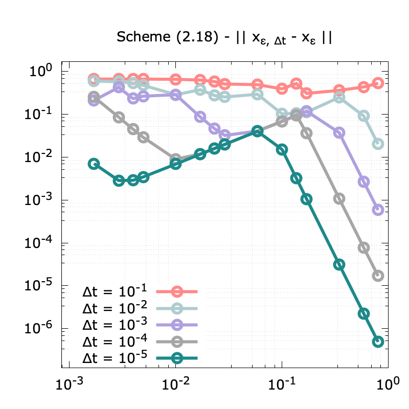
In Figure 4.1, we present the numerical error on ‖𝐱ε,Δ​t−𝐱ε‖\|\mathbf{x}_{\varepsilon,\Delta t}-\mathbf{x}_{\varepsilon}\| expressed with respect to ε\varepsilon in log-log scale for various time steps Δ​t∈{10−5,⋯,10−1}\Delta t\in\{10^{-5},\cdots,10^{-1}\}. When ε≥10−1\varepsilon\geq 10^{-1}, we observe the expected second order accuracy of the different schemes. However, as ε\varepsilon becomes smaller, the time steps are too large and the numerical error for both schemes (2.9) and (2.18) increases. In contrast, the numerical error associated to the modified Crank-Nicolson scheme (3.2) and the IMEX2L [10] decreases with respect to ε\varepsilon. This behavior is typical of an asymptotic preserving scheme for which the error becomes of order ε\varepsilon when the time step Δ​t\Delta t is sufficiently large. It is worth mentioning that the behavior of the errors for (3.2) and the IMEX2L differs significantly as ε≪1\varepsilon\ll 1. Indeed, even with a large time step the modified Crank-Nicolson scheme (3.2) remains so accurate that the error of order Δ​t2\Delta t^{2} is negligible compared to the error with respect to ε\varepsilon. This phenomena can also be observed in Figures 4.2 and 4.3, where we report the errors compared to the reference solution of the asymptotic model ‖𝐱ε,Δ​t−𝐲‖\|\mathbf{x}_{\varepsilon,\Delta t}-\mathbf{y}\| and ‖eε,Δ​t−g‖\|e_{\varepsilon,\Delta t}-g\|. Clearly the schemes (2.9) and (2.18) do not capture a consistent approximation (𝐲,g)(\mathbf{y},g) to the asymptotic solutions (1.8) as ε→0\varepsilon\rightarrow 0. These numerical experiments illustrate the lack of consistency proven in Propositions 2.2 and 2.3. In contrast, both schemes (3.2) and the IMEX2L, based on the approximation of the augmented system (1.6), successfully capture the limit with the correct convergence rate with respect to ε\varepsilon (slope of order one). The advantage of the scheme (3.2) is that, when ε≪1\varepsilon\ll 1, the amplitude of the numerical error is much smaller than the one corresponding to other schemes.

Refer to caption
Refer to caption
Refer to caption
Refer to caption
Figure 4.1. One single particle motion: Numerical errors of discrete solution 𝐱ε,Δ​t\mathbf{x}_{\varepsilon,\Delta t}, approximated by several schemes: (2.9), (2.18), IMEX2L and (3.2), with reference solution 𝐱ε\mathbf{x}_{\varepsilon} of (1.4) for various ε>0\varepsilon>0 and Δ​t>0\Delta t>0.
Refer to caption
Refer to caption
Refer to caption
Refer to caption
Figure 4.2. One single particle motion: Numerical errors of discrete solution 𝐱ε,Δ​t\mathbf{x}_{\varepsilon,\Delta t}, approximated by several schemes: (2.9), (2.18), IMEX2L and (3.2), with guiding center solution 𝐲\mathbf{y} of (1.8) for various ε>0\varepsilon>0 and Δ​t>0\Delta t>0.
Refer to caption
Refer to caption
Refer to caption
Refer to caption
Figure 4.3. One single particle motion: Numerical errors of discrete solution eε,Δ​te_{\varepsilon,\Delta t}, approximated by several schemes: (2.9), (2.18), IMEX2L and (3.2), with guiding center solution gg of (1.8) for various ε>0\varepsilon>0 and Δ​t>0\Delta t>0.

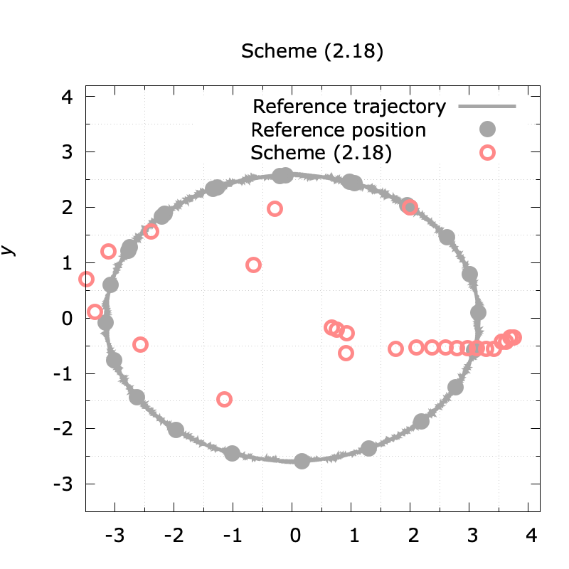
To illustrate this point, we also present the space trajectories corresponding to ε=0.01\varepsilon=0.01 and Δ​t=0.1\Delta t=0.1 for large time simulations (with T=30T=30). In Figure 4.4, we observe that the particle trajectory forms a circular motion under the effect of both drifts 𝐄⟂/b\mathbf{E}^{\perp}/b and ∇𝐱⟂b/b2\nabla_{\mathbf{x}}^{\perp}b/b^{2}, which appear explicitly in the asymptotic model (1.8). The scheme (3.2) provides an approximation close to the reference solution, while other schemes fail to get the correct position of the particle, since they do not capture correctly the drift ∇𝐱⟂b/b2\nabla_{\mathbf{x}}^{\perp}b/b^{2} in the limit ε→0\varepsilon\rightarrow 0.

Refer to caption
Refer to caption
Refer to caption
Refer to caption
Figure 4.4. One single particle motion: Trajectory of particle approximated by several schemes: (2.9), (2.18), IMEX2L and (3.2) with ε=0.01\varepsilon=0.01, Δ​t=0.1\Delta t=0.1 and final time T=30​sT=30s.

Furthermore, from the results presented in Figure 4.5, we observe that the IMEX2L and (3.2) schemes accurately track the variations in kinetic and potential energy over a long period, unlike (2.9) and (2.18).

Refer to caption
Refer to caption
Refer to caption
Refer to caption
Figure 4.5. One single particle motion: Variation of energy approximated by several schemes: (2.9), (2.18), IMEX2L and (3.2) with ε=0.01\varepsilon=0.01, Δ​t=0.1\Delta t=0.1 and final time T=30​sT=30s.

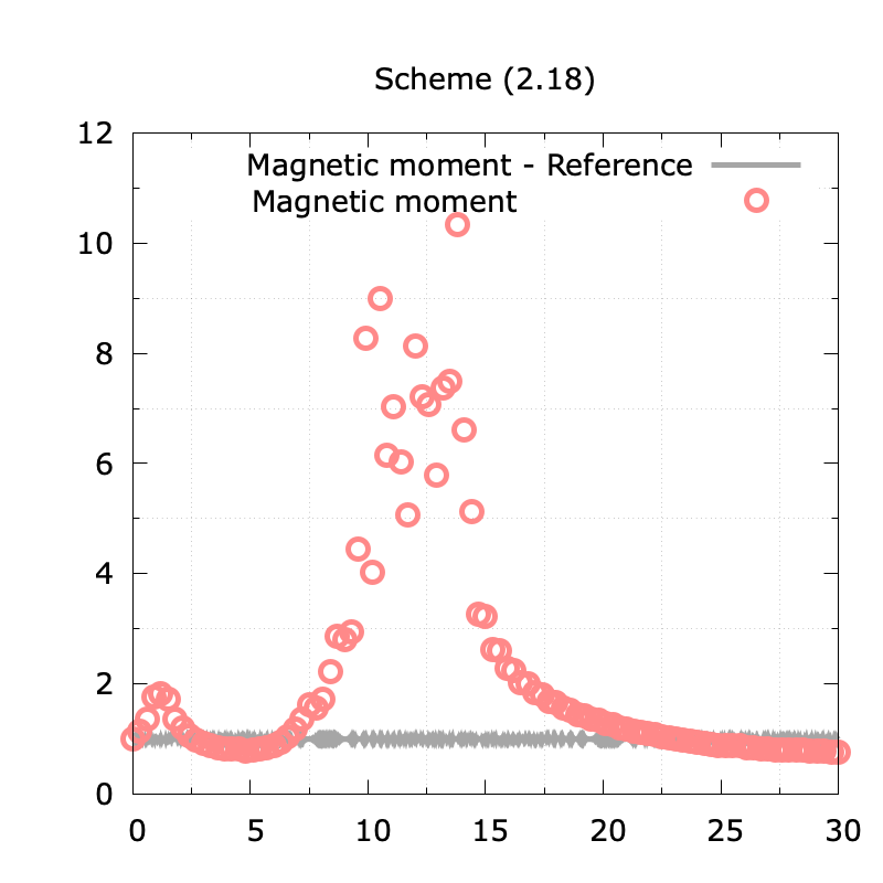
Finally, the time evolution of the magnetic moment approximation is presented and compared with a reference solution in Figure 4.6. Let us emphasize that only the modified scheme (3.2) accurately describes the amplitude of the fast oscillations of με\mu_{\varepsilon} compared to the other schemes. Indeed, even if the time step Δ​t\Delta t is much larger than the fastest time scale of order ε2\varepsilon^{2}, the quantity με,Δ​t\mu_{\varepsilon,\Delta t} oscillates with the correct amplitude of order ε2\varepsilon^{2}.

Refer to caption
Refer to caption
Refer to caption
Refer to caption
Figure 4.6. One single particle motion: Evolution of magnetic moment approximated by several schemes: (2.9), (2.18), IMEX2L and (3.2) with ε=0.01\varepsilon=0.01, Δ​t=0.1\Delta t=0.1 and final time T=30​sT=30s.

As a conclusion, for the single particle motion, the modified Crank-Nicolson scheme (3.2) is much more accurate than the schemes (2.9), (2.18) or IMEX2L, even when ε≪1\varepsilon\ll 1, with a time step Δ​t\Delta t independent of ε\varepsilon. These elementary numerical simulations confirm the ability of the modified Crank-Nicolson scheme (3.2) to capture the evolution of the ”slow” variables (𝐱ε,eε)({\mathbf{x}}_{\varepsilon},e_{\varepsilon}) uniformly with respect to ε\varepsilon by essentially transitioning automatically to the guiding center motion (1.8) when it is not enable anymore to follow the fast oscillations of the initial system.

4.2. Vlasov-Poisson system

We now consider the Vlasov-Poisson system (1.3) on a domain Ω⊂ℝ2\Omega\subset\mathbb{R}^{2}, assuming that the density is concentrated far from the boundary. The Poisson equation is solved with homogeneous Dirichlet boundary conditions using a classical five points second order finite difference method with ghost points to take into account the effect of the boundary conditions [15].

For each time t≥0t\geq 0, we may define the total energy ℰε​(t){\mathcal{E}}_{\varepsilon}(t) as

(4.3) ℰε​(t):=𝐊ε​(t)+𝐔ε​(t),\displaystyle{\mathcal{E}}_{\varepsilon}(t)\,\,:=\,\,{\mathbf{K}}_{\varepsilon}(t)\,+\,{\mathbf{U}}_{\varepsilon}(t),

where the kinetic energy 𝐊ε​(t){\mathbf{K}}_{\varepsilon}(t) and the potential energy 𝐔ε​(t){\mathbf{U}}_{\varepsilon}(t) are given by

{𝐊ε​(t):=12​∫Ω∫ℝ2fε​(t,𝐱,𝐯)​‖𝐯‖2​d𝐯​d𝐱,𝐔ε​(t):=12​∫Ω‖𝐄ε​(t,𝐱)‖2​d𝐱.\left\{\begin{array}[]{l}\displaystyle{\mathbf{K}}_{\varepsilon}(t)\,:=\,\frac{1}{2}\int\limits_{\Omega}\int\limits_{\mathbb{R}^{2}}f_{\varepsilon}(t,\mathbf{x},\mathbf{v})\,\|\mathbf{v}\|^{2}\,\mathrm{d}\mathbf{v}\,\mathrm{d}\mathbf{x},\\[8.99994pt] \displaystyle{\mathbf{U}}_{\varepsilon}(t)\,:=\,\frac{1}{2}\int\limits_{\Omega}\|\mathbf{E}_{\varepsilon}(t,\mathbf{x})\|^{2}\,\mathrm{d}\mathbf{x}\,.\end{array}\right.

Assuming that the distribution function is compactly supported in the open set Ω\Omega, the total energy ℰε​(t){\mathcal{E}}_{\varepsilon}(t) is conserved for all time t≥0t\geq 0.

We also define the magnetic moment for the Vlasov-Poisson system (1.3) given by

(4.4) με​(t):=12​∫Ω∫ℝ2fε​(t,𝐱,𝐯)​‖𝐯‖2b​(𝐱)​d𝐯​d𝐱,t≥0\displaystyle\mu_{\varepsilon}(t)\,:=\,\frac{1}{2}\,\int\limits_{\Omega}\int\limits_{\mathbb{R}^{2}}f_{\varepsilon}(t,\mathbf{x},\mathbf{v})\dfrac{\|\mathbf{v}\|^{2}}{b(\mathbf{x})}\,\mathrm{d}\mathbf{v}\,\mathrm{d}\mathbf{x},\qquad t\geq 0

and expect that με​(t)\mu_{\varepsilon}(t) is an invariant in time in the asymptotic limit ε→0\varepsilon\rightarrow 0 for the limit model (1.8).

For this section, we performed numerical experiments using the modified Crank-Nicolson scheme (3.2) to approximate the particles trajectory corresponding to the Vlasov equation. Despite the fact that the modified Crank-Nicolson scheme (3.2) does not conserves exactly the total energy, we expect that its variations are of order 𝒪​(Δ​t2){\mathcal{O}}(\Delta t^{2}) even when ε\varepsilon tends to zero. Furthermore, the modified Crank-Nicolson scheme (3.2) should capture correctly the asymptotic limit ε→0\varepsilon\rightarrow 0, as it has been shown for the single particle motion.

4.2.1. Diocotron instability

We first consider Vlasov-Poisson system (1.3) set in a disk Ω=D​(0,12)\Omega=D(0,12) centered at the origin with a radius R=12R=12 and a uniform grid of the square (−12,12)2(-12,12)^{2} with Δ​𝐱=0.1\Delta{\mathbf{x}}=0.1. The simulation starts with a Maxwellian distribution in velocity, whose macroscopic density is a perturbed uniform distribution in an annulus. More precisely, we choose

f​(0,𝐱,𝐯)=ρ0​(𝐱)2​π​exp⁡(−‖𝐯‖22),f(0,\mathbf{x},\mathbf{v})\,=\,\dfrac{\rho_{0}(\mathbf{x})}{2\pi}\,\exp\left(-\frac{\|\mathbf{v}\|^{2}}{2}\right),

where ρ0\rho_{0} is given by

ρ0​(𝐱)={n0​(1+α​cos⁡(7​θ)),for​  6≤‖𝐱‖≤7,0,else,\displaystyle\rho_{0}(\mathbf{x})=\left\{\begin{array}[]{l}n_{0}(1\,+\,\alpha\,\cos(7\theta)),\,\,{\rm for}\,\,6\leq\|\mathbf{x}\|\leq 7\,,\\[8.99994pt] 0,\,\,{\rm else,}\end{array}\right.

in which n0=0.25n_{0}=0.25, α=0.001\alpha=0.001, and the angle θ\theta is defined as θ=arctan⁡(x2/x1)\theta=\arctan(x_{2}/x_{1}) with 𝐱=(x1,x2)\mathbf{x}=(x_{1},x_{2}). Moreover, we consider strong external magnetic field which is given by

b​(t,𝐱)=20400−‖𝐱‖2.b(t,\mathbf{x})=\dfrac{20}{\sqrt{400-\|{\mathbf{x}}\|^{2}}}.

Since bb is not homogeneous, even in the asymptotic regime the kinetic and potential parts of the total energy are not preserved separately, but the total energy corresponding to the Vlasov–Poisson system is still preserved. Figure 4.7 shows that all these features are captured satisfactorily by the modified Crank-Nicolson scheme (3.2) even on long time evolutions with a large time step Δ​t=0.1\Delta t=0.1 and small ε=10−2\varepsilon=10^{-2}. On the one hand, the variations of the total energy have an amplitude of order 10−410^{-4}, which is satisfying compared to the physical variations of the potential and kinetic energy of order 2× 10−22\times\,10^{-2}. On the other hand, the quantity με\mu_{\varepsilon} also varies around 10−410^{-4}, which corresponds to the scale of ε2=10−4\varepsilon^{2}=10^{-4}. This phenomena has already been observed for the single particle motion and will be discussed below.

Refer to caption
Refer to caption
Figure 4.7. Diocotron instability: Time evolution of the variations of the relative potential 𝐔ε{\mathbf{U}}_{\varepsilon} and kinetic energy 𝐊ε{\mathbf{K}}_{\varepsilon} (left) and magnetic moment με\mu_{\varepsilon} (right) with ε=10−2\varepsilon=10^{-2} and (Δ​t,Δ​𝐱)=(0.1,0.1)(\Delta t,\Delta{\mathbf{x}})=(0.1,0.1), using the modified Crank-Nicolson scheme (3.2).

In Figure 4.8, we visualize the corresponding dynamics by presenting several snapshots of the macroscopic density at some specific times t=0t=0, 5050, 100100 and 150150. The numerical results obtained with our PIC methods are in good agreements with those obtained with a finite difference scheme [15] for the asymptotic model (1.11).

Refer to caption
Refer to caption
Refer to caption
Refer to caption
Figure 4.8. Diocotron instability: Macroscopic density evolution at some specific time T=0,50,100,150T=0,50,100,150 with ε=10−2\varepsilon=10^{-2} and (Δ​t,Δ​𝐱)=(0.1,0.1)(\Delta t,\Delta{\mathbf{x}})=(0.1,0.1), using the modified Crank-Nicolson scheme (3.2).

Furthermore, we performed simulations for various ε∈{10−2, 5. 10−2, 10−1}\varepsilon\in\{10^{-2},\,5.\,10^{-2},\,10^{-1}\}, shown in Figure 4.9. On the left hand side, we report the total energy variations, which are theoretically of order Δ​t2\Delta t^{2}. However, when ε\varepsilon is small these variations decrease so that the total energy is well preserved in the limit ε→0\varepsilon\to 0. On the right hand side, we present the variations of the adiabatic invariant με\mu_{\varepsilon}, which is not preserved by the solution to the Vlasov-Poisson system but only by the asymptotic model (1.11). Here, we notice that this quantity oscillates with an amplitude of order ε2\varepsilon^{2}. Surprisingly, even with a large time step Δ​t\Delta t, the numerical scheme (3.2) is able to capture the correct amplitude. This can also observed on the variations of both the potential and the kinetic energy in Figures 4.7. The slow variations definitively correspond to the effect of the drifts 𝐄⟂/b\mathbf{E}^{\perp}/b and ∇𝐱⟂b/b2\nabla_{\mathbf{x}}^{\perp}b/b^{2}, but the fast oscillations and their amplitudes are more intricate. In order to verify that these small oscillations are not a numerical artefact, we compute a reference solution with a small time step for ε=10−1\varepsilon=10^{-1} and 10−210^{-2} and compare these results with the those obtained from (3.2) with Δ​t=0.1\Delta t=0.1. Figure 4.10 clearly indicates that with such a time step, the scheme (3.2) described accurately the amplitude of these fast oscillations. However, since Δ​t\Delta t is much larger than the oscillation period, the modified scheme can not describe the physical frequency.

Refer to caption
Refer to caption
Figure 4.9. Diocotron instability: Time evolution of the variations of the relative total energy ℰε{\mathcal{E}}_{\varepsilon} (left) and magnetic moment με\mu_{\varepsilon} (right) with different ε=10−1\varepsilon=10^{-1}, 5. 10−25.\,10^{-2} and 10−210^{-2} with (Δ​t,Δ​𝐱)=(0.1,0.1)(\Delta t,\Delta{\mathbf{x}})=(0.1,0.1), using the modified Crank-Nicolson scheme (3.2).
Refer to caption
Refer to caption
Figure 4.10. Diocotron instability: Time evolution of the variation of the potential energy 𝐔ε{\mathbf{U}}_{\varepsilon} in a short time interval with ε=0.1\varepsilon=0.1 (left) and ε=0.01\varepsilon=0.01 (right) using the modified Crank-Nicolson scheme (3.2).

4.2.2. Vortex interaction

Finally we consider Vlasov-Poisson system (1.3) in a D-Shaped domain Ω⊂ℝ2\Omega\subset\mathbb{R}^{2}, described by a mapping from polar coordinates (r,θ)(r,\theta) to Cartesian coordinates 𝐱=(x1,x2)\mathbf{x}=(x_{1},x_{2}) given by

{x1=a+r​cos⁡(θ+arcsin⁡(0.416)​sin⁡(θ)),x2=b+ 1.66​r​sin⁡(θ),\displaystyle\begin{dcases}\displaystyle x_{1}\,=\,a\,+\,r\,\cos\left(\theta+\arcsin(0.416)\,\sin(\theta)\right)\,,\\ \displaystyle x_{2}\,=\,b\,+\,1.66\,r\,\sin(\theta)\,,\end{dcases}

centered at the origin (a,b)=(0,0)(a,b)=(0,0) where 0<r≤100<r\leq 10 and 0≤θ≤2​π0\leq\theta\leq 2\pi. Then we consider a uniform grid of the rectangle (−11,11)×(−17,17)(-11,11)\times(-17,17) with a space discretization Δ​𝐱=0.1\Delta{\mathbf{x}}=0.1. We choose the initial distribution function such that

(4.5) f​(0,𝐱,𝐯)=58​π2​[exp⁡(−‖𝐱−𝐱0‖22)+exp⁡(−‖𝐱+𝐱0‖22)]​exp⁡(−‖𝐯‖22),f(0,\mathbf{x},\mathbf{v})\,=\,\dfrac{5}{8\pi^{2}}\left[\exp\left(-\dfrac{\|\mathbf{x}-\mathbf{x}_{0}\|^{2}}{2}\right)\,+\,\exp\left(-\dfrac{\|\mathbf{x}+\mathbf{x}_{0}\|^{2}}{2}\right)\right]\,\exp\left(-\dfrac{\|\mathbf{v}\|^{2}}{2}\right),

with 𝐱0=(1.5,−1.5)\mathbf{x}_{0}=(1.5,-1.5). Moreover, we consider a non homogeneous external magnetic field such as

b​(t,𝐱)=20400−x12−x22.b(t,\mathbf{x})\,=\,\dfrac{20}{\sqrt{400-x_{1}^{2}-x_{2}^{2}}}\,.

As expected for such a configuration, since bb is not homogeneous, even in the asymptotic regime the kinetic and potential parts of the total energy are not preserved separately, but the total energy corresponding to the Vlasov–Poisson system is still preserved. In addition, the quantity με\mu_{\varepsilon} is an invariant for the guiding center model but oscillates with a high frequency for the Vlasov-Poisson system with a small amplitude. Indeed, Figure 4.11 shows that all these features are again captured by the scheme (3.2) even on long time evolutions with a large time step. Furthermore, in Figure 4.12, we visualize the corresponding dynamics by presenting several snapshots of the time evolution of the macroscopic charge density for ε=10−2\varepsilon=10^{-2} at time t=0t=0, 8080, 160160, 240240, 320320 and 400400. Since ε≪1\varepsilon\ll 1, the conservation of e/b​(𝐱)e/b({\mathbf{x}}) offers coercivity jointly in (𝐱,e)({\mathbf{x}},e) allowing to confine the density in the D-shape domain. Such a confinement is indeed observed, jointly with the expected eventual merging of two initial vortices in a relatively short time. We also observe small filaments at low density, which generate a ”halo” propagating into the domain as already observed in [15]. Finally, from Figure 4.13, similarly to diocotron instability experiment in Section 4.2.1, the relative variations of the total energy ℰε{\mathcal{E}}_{\varepsilon} and the adiabatic invariant με\mu_{\varepsilon} show the ability of preserving these parameters (ℰε,με)({\mathcal{E}}_{\varepsilon},\mu_{\varepsilon}) in the limit ε→0\varepsilon\to 0.

Refer to caption
Refer to caption
Figure 4.11. Vortex interaction: Time evolution of the variations of the relative potential 𝐔ε{\mathbf{U}}_{\varepsilon} and kinetic energy 𝐊ε{\mathbf{K}}_{\varepsilon} (left) and magnetic moment με\mu_{\varepsilon} (right) with ε=10−2\varepsilon=10^{-2} with (Δ​t,Δ​𝐱)=(0.1,0.1)(\Delta t,\Delta{\mathbf{x}})=(0.1,0.1), using the modified Crank-Nicolson scheme (3.2).
Refer to caption
Refer to caption
Refer to caption
Refer to caption
Refer to caption
Refer to caption
Figure 4.12. Vortex interaction: Macroscopic density evolution at some specific time TT with ε=10−2\varepsilon=10^{-2} with (Δ​t,Δ​𝐱)=(0.1,0.1)(\Delta t,\Delta{\mathbf{x}})=(0.1,0.1), using the modified Crank-Nicolson scheme (3.2).
Refer to caption
Refer to caption
Figure 4.13. Vortex interaction: Time evolution of the variations of the relative total energy ℰε{\mathcal{E}}_{\varepsilon} (left) and magnetic moment με\mu_{\varepsilon} (right) with different ε=10−1\varepsilon=10^{-1}, 5. 10−25.\,10^{-2} and 10−210^{-2} and (Δ​t,Δ​𝐱)=(0.1,0.1)(\Delta t,\Delta{\mathbf{x}})=(0.1,0.1), using the modified Crank-Nicolson scheme (3.2).

In summary, the modified Crank-Nicolson scheme (3.2) integrated into Particle-In-Cell method shows consistency and stability of long time simulations with a coarse time step, even for small ε≪1\varepsilon\ll 1. Moreover, the solutions (ℰε,με)({\mathcal{E}}_{\varepsilon},\mu_{\varepsilon}) of these numerical tests preserve the structure of the limit system ε→0\varepsilon\to 0 and provide accurately the amplitude of these variations.

5. Conclusion

In this paper, we propose a modified Crank-Nicolson time discretization technique for Particle-In-Cell simulations. Our approach guarantees the accuracy and stability of small-scale variables, even when the magnetic field amplitude becomes large, thus correctly capturing their long-term behavior, including in cases of inhomogeneous magnetic fields and coarse time grids. Comparison with previous contributions on Crank-Nicolson and semi-implicit schemes demonstrates the effectiveness of our approach, with accuracy improving by several orders of magnitude. Even for large-time simulations, the resulting numerical schemes provide acceptable accuracy on physical invariants (total energy for all ε\varepsilon, magnetic moment when ε≪1\varepsilon\ll 1), while fast scales are automatically filtered when the time step is large compared to ε2\varepsilon^{2}.

As a theoretical validation, we have proven that, under certain stability assumptions on the numerical approximations, the slow part of the approximation converges, when ε→0\varepsilon\to 0, to the solution of a limit scheme of asymptotic evolution, preserving the initial order of precision. A complete analytical study (including proofs of stability), in the spirit of [14], is currently under investigation [13].

From a practical point of view, the next natural step would be extensions to realistic, genuinely three-dimensional geometries in the spirit of [12].

Appendix A Formal asymptotic behavior for a given electromagnetic field

For the convenience of the reader, we provide here the main algebraic manipulations of equations (1.4) leading to the guiding-center system (1.8). The system is well-known and no details of the derivation is needed in the rest of the paper but consistency with (1.8) is crucially used in our evaluations of numerical schemes.

To begin with, in order to eliminate ε−1​𝐯ε\varepsilon^{-1}{\mathbf{v}}_{\varepsilon} from (1.6), we observe that equation (1.7) may be replaced with

(A.1) ε​dd​t​(𝐯ε⟂b​(𝐱ε))=𝐄⟂​(𝐱ε)b​(𝐱ε)−(∇𝐱b​(𝐱ε)b2​(𝐱ε)⋅𝐯ε)​𝐯ε⟂+𝐯εε.\varepsilon\,\dfrac{\mathrm{d}}{\mathrm{d}t}\left(\dfrac{\mathbf{v}_{\varepsilon}^{\perp}}{b(\mathbf{x}_{\varepsilon})}\right)\,=\,\dfrac{\mathbf{E}^{\perp}(\mathbf{x}_{\varepsilon})}{b(\mathbf{x}_{\varepsilon})}\,-\,\left(\dfrac{\nabla_{\mathbf{x}}b(\mathbf{x}_{\varepsilon})}{b^{2}(\mathbf{x}_{\varepsilon})}\cdot\mathbf{v}_{\varepsilon}\right)\,\mathbf{v}_{\varepsilon}^{\perp}\,+\,\dfrac{\mathbf{v}_{\varepsilon}}{\varepsilon}\,.

In order to characterize the asymptotic dynamics of the slow variables (𝐱ε,eε)(\mathbf{x}_{\varepsilon},e_{\varepsilon}) when ε→0\varepsilon\rightarrow 0, we notice that their equations depend linearly on 𝐯ε{\mathbf{v}}_{\varepsilon}, hence as in [11] we write for all t∈ℝ+t\in{\mathbb{R}}^{+} and any linear operator 𝐋​(t){\mathbf{L}}(t)

ε​dd​t​(𝐋​(t)​𝐯ε⟂b​(𝐱ε))=ε​d​𝐋​(t)d​t​𝐯ε⟂b​(𝐱ε)+𝐋​(t)​(𝐄⟂​(𝐱ε)b​(𝐱ε)−(∇𝐱b​(𝐱ε)b2​(𝐱ε)⋅𝐯ε)​𝐯ε⟂+𝐯εε).\varepsilon\,\dfrac{\mathrm{d}}{\mathrm{d}t}\left({\mathbf{L}}(t)\frac{\mathbf{v}_{\varepsilon}^{\perp}}{b({\mathbf{x}}_{\varepsilon})}\right)\,=\,\varepsilon\dfrac{\mathrm{d}{\mathbf{L}}(t)}{\mathrm{d}t}\,\frac{\mathbf{v}_{\varepsilon}^{\perp}}{b({\mathbf{x}}_{\varepsilon})}\,+\,{\mathbf{L}}(t)\left(\frac{\mathbf{E}^{\perp}(\mathbf{x}_{\varepsilon})}{b(\mathbf{x}_{\varepsilon})}\,-\,\left(\frac{\nabla_{\mathbf{x}}b(\mathbf{x}_{\varepsilon})}{b^{2}(\mathbf{x}_{\varepsilon})}\cdot{\mathbf{v}}_{\varepsilon}\right)\,{\mathbf{v}}_{\varepsilon}^{\perp}\,+\,\frac{\mathbf{v}_{\varepsilon}}{\varepsilon}\right)\,.

Therefore, applying the latter to 𝐋𝐱​(t):𝐮∈ℝ2↦𝐮∈ℝ2\mathbf{L}_{\mathbf{x}}(t):\mathbf{u}\in\mathbb{R}^{2}\mapsto\mathbf{u}\in\mathbb{R}^{2} and 𝐋e​(t):𝐮∈ℝ2↦𝐄​(𝐱ε)⋅𝐮∈ℝ\mathbf{L}_{e}(t):\mathbf{u}\in\mathbb{R}^{2}\mapsto\mathbf{E}(\mathbf{x}_{\varepsilon})\cdot\mathbf{u}\in\mathbb{R} and inserting the outcome into the system of slow variables (1.6), we obtain

(A.2) {dd​t​(𝐱ε−ε​𝐯ε⟂b​(𝐱ε))=−𝐄⟂​(𝐱ε)b​(𝐱ε)+(∇𝐱b​(𝐱ε)b2​(𝐱ε)⋅𝐯ε)​𝐯ε⟂,dd​t​(eε−ε​𝐄​(𝐱ε)⋅𝐯ε⟂b​(𝐱ε))=−(𝐯ε​∇𝐱)​(𝐄b)​(𝐱ε)⋅𝐯ε⟂.\left\{\begin{array}[]{l}\displaystyle\dfrac{\mathrm{d}}{\mathrm{d}t}\left(\mathbf{x}_{\varepsilon}-\varepsilon\,\dfrac{\mathbf{v}_{\varepsilon}^{\perp}}{b(\mathbf{x}_{\varepsilon})}\right)\,=\,-\dfrac{\mathbf{E}^{\perp}(\mathbf{x}_{\varepsilon})}{b(\mathbf{x}_{\varepsilon})}\,+\,\left(\dfrac{\nabla_{\mathbf{x}}b(\mathbf{x}_{\varepsilon})}{b^{2}(\mathbf{x}_{\varepsilon})}\cdot\mathbf{v}_{\varepsilon}\right)\,\mathbf{v}_{\varepsilon}^{\perp},\\[11.99998pt] \displaystyle\dfrac{\mathrm{d}}{\mathrm{d}t}\left(e_{\varepsilon}-\varepsilon\,\mathbf{E}(\mathbf{x}_{\varepsilon})\cdot\dfrac{\mathbf{v}_{\varepsilon}^{\perp}}{b(\mathbf{x}_{\varepsilon})}\right)\,=\,-\left(\mathbf{v}_{\varepsilon}\,\nabla_{\mathbf{x}}\right)\left(\dfrac{\mathbf{E}}{b}\right)(\mathbf{x}_{\varepsilon})\cdot\,\mathbf{v}^{\perp}_{\varepsilon}\,.\end{array}\right.

This latter system may replace (1.6) and is not stiff with respect to ε≪1\varepsilon\ll 1, but it also suggests the introduction of new variables, as the guiding center variable 𝐱ε−ε​𝐯ε⟂/b​(𝐱ε)\mathbf{x}_{\varepsilon}-\varepsilon\,{\mathbf{v}_{\varepsilon}^{\perp}}/{b(\mathbf{x}_{\varepsilon})}. However, these new equations still involve at leading order quadratic terms in 𝐯ε\mathbf{v}_{\varepsilon} on the right hand side. Hence, following [11], we turn our attention to bilinear operators 𝐀​(t)\mathbf{A}(t) and derive

ε2​dd​t​(𝐀​(t)​(𝐯ε,𝐯ε⟂b​(𝐱ε)))\displaystyle\varepsilon^{2}\dfrac{\mathrm{d}}{\mathrm{d}t}\left(\mathbf{A}(t)\left(\mathbf{v}_{\varepsilon},\dfrac{\mathbf{v}_{\varepsilon}^{\perp}}{b({\mathbf{x}}_{\varepsilon})}\right)\right) =\displaystyle= ε2​d​𝐀​(t)d​t​(𝐯ε,𝐯ε⟂b​(𝐱ε))+ε​𝐀​(t)​(𝐄​(𝐱ε)b​(𝐱ε),𝐯ε⟂)\displaystyle\varepsilon^{2}\dfrac{\mathrm{d}\mathbf{A}(t)}{\mathrm{d}t}\left(\mathbf{v}_{\varepsilon}\,,\dfrac{\mathbf{v}_{\varepsilon}^{\perp}}{b({\mathbf{x}}_{\varepsilon})}\right)+\varepsilon\mathbf{A}(t)\left(\frac{\mathbf{E}(\mathbf{x}_{\varepsilon})}{b({\mathbf{x}}_{\varepsilon})}\,,\mathbf{v}_{\varepsilon}^{\perp}\right)
+\displaystyle+ ε​𝐀​(t)​(𝐯ε,𝐄⟂​(𝐱ε)b​(𝐱ε))−ε​(∇𝐱b​(𝐱ε)b2​(𝐱ε)⋅𝐯ε)​𝐀​(t)​(𝐯ε,𝐯ε⟂)\displaystyle\varepsilon\mathbf{A}(t)\left(\mathbf{v}_{\varepsilon}\,,\frac{\mathbf{E}^{\perp}(\mathbf{x}_{\varepsilon})}{b({\mathbf{x}}_{\varepsilon})}\right)-\varepsilon\,\left(\frac{\nabla_{\mathbf{x}}b(\mathbf{x}_{\varepsilon})}{b^{2}(\mathbf{x}_{\varepsilon})}\cdot{\mathbf{v}}_{\varepsilon}\right)\,\mathbf{A}(t)(\mathbf{v}_{\varepsilon},\mathbf{v}_{\varepsilon}^{\perp})
−\displaystyle- 𝐀​(t)​(𝐯ε⟂,𝐯ε⟂)+𝐀​(t)​(𝐯ε,𝐯ε).\displaystyle\mathbf{A}(t)(\mathbf{v}_{\varepsilon}^{\perp},\mathbf{v}_{\varepsilon}^{\perp})+\mathbf{A}(t)(\mathbf{v}_{\varepsilon},\mathbf{v}_{\varepsilon}).

Since (𝐯ε,𝐯ε⟂)(\mathbf{v}_{\varepsilon},\mathbf{v}_{\varepsilon}^{\perp}) is an orthogonal basis of ℝ2\mathbb{R}^{2} (when 𝐯ε{\mathbf{v}}_{\varepsilon} is non zero), introducing the operator Tr{\rm Tr} one observes that

‖𝐯ε‖2​Tr​(𝐀​(t))=𝐀​(t)​(𝐯ε⟂,𝐯ε⟂)+𝐀​(t)​(𝐯ε,𝐯ε).\displaystyle\|\mathbf{v}_{\varepsilon}\|^{2}\,{\rm Tr}(\mathbf{A}(t))\,=\,\mathbf{A}(t)(\mathbf{v}_{\varepsilon}^{\perp},\mathbf{v}_{\varepsilon}^{\perp})\,+\,\mathbf{A}(t)(\mathbf{v}_{\varepsilon},\mathbf{v}_{\varepsilon})\,.

Therefore, one may reformulate (A) as

𝐀​(t)​(𝐯ε,𝐯ε)=12​‖𝐯ε‖2​Tr​(𝐀​(t))+ε2​d​κ𝐀d​t​(t,𝐱ε,𝐯ε)+ε​η𝐀​(t,𝐱ε,𝐯ε),\mathbf{A}(t)(\mathbf{v}_{\varepsilon},\mathbf{v}_{\varepsilon})\,=\,\dfrac{1}{2}\,\|\mathbf{v}_{\varepsilon}\|^{2}\,{\rm Tr}(\mathbf{A}(t))\,+\,\varepsilon^{2}\,\dfrac{\mathrm{d}\kappa_{\mathbf{A}}}{\mathrm{d}t}(t,\mathbf{x}_{\varepsilon},\mathbf{v}_{\varepsilon})\,+\,\varepsilon\,\eta_{\mathbf{A}}(t,\mathbf{x}_{\varepsilon},\mathbf{v}_{\varepsilon})\,,

where κ𝐀\kappa_{\mathbf{A}} and η𝐀\eta_{\mathbf{A}} are given by

{κ𝐀​(t,𝐱ε,𝐯ε)=12​𝐀​(t)​(𝐯ε,𝐯ε⟂b​(𝐱ε)),η𝐀​(t,𝐱ε,𝐯ε)=∇𝐱b​(𝐱ε)2​b2​(𝐱ε)⋅𝐯ε​𝐀​(t)​(𝐯ε,𝐯ε⟂)−ε2​d​𝐀​(t)d​t​(𝐯ε,𝐯ε⟂b​(𝐱ε))−12​(𝐀​(t)​(𝐄​(𝐱ε)b​(𝐱ε),𝐯ε⟂)+𝐀​(t)​(𝐯ε,𝐄⟂​(𝐱ε)b​(𝐱ε))).\left\{\begin{array}[]{l}\displaystyle\kappa_{\mathbf{A}}(t,\mathbf{x}_{\varepsilon},\mathbf{v}_{\varepsilon})\,=\,\dfrac{1}{2}\,\mathbf{A}(t)\left(\mathbf{v}_{\varepsilon},\dfrac{\mathbf{v}_{\varepsilon}^{\perp}}{b(\mathbf{x}_{\varepsilon})}\right),\\[8.99994pt] \displaystyle\eta_{\mathbf{A}}(t,\mathbf{x}_{\varepsilon},\mathbf{v}_{\varepsilon})\,=\,\dfrac{\nabla_{\mathbf{x}}b({\mathbf{x}}_{\varepsilon})}{2\,b^{2}({\mathbf{x}}_{\varepsilon})}\cdot\mathbf{v}_{\varepsilon}\,\mathbf{A}(t)\left(\mathbf{v}_{\varepsilon},\mathbf{v}_{\varepsilon}^{\perp}\right)\,-\,\frac{\varepsilon}{2}\,\frac{\mathrm{d}\mathbf{A}(t)}{\mathrm{d}t}\left(\mathbf{v}_{\varepsilon},\dfrac{\mathbf{v}_{\varepsilon}^{\perp}}{b(\mathbf{x}_{\varepsilon})}\right)\\[8.99994pt] \qquad\qquad\qquad\displaystyle-\frac{1}{2}\left(\mathbf{A}(t)\left(\frac{\mathbf{E}(\mathbf{x}_{\varepsilon})}{b({\mathbf{x}}_{\varepsilon})},\mathbf{v}_{\varepsilon}^{\perp}\right)\,+\,\mathbf{A}(t)\left(\mathbf{v}_{\varepsilon},\dfrac{\mathbf{E}^{\perp}(\mathbf{x}_{\varepsilon})}{b(\mathbf{x}_{\varepsilon})}\right)\right)\,.\end{array}\right.

To apply the latter to the bilinear maps 𝐀𝐱​(t):(𝐮1,𝐮2)∈ℝ2×ℝ2↦𝐮2⟂​∇𝐱b​(𝐱ε)b2​(𝐱ε)⋅𝐮1∈ℝ2\mathbf{A}_{\mathbf{x}}(t):(\mathbf{u}_{1},\mathbf{u}_{2})\in\mathbb{R}^{2}\times\mathbb{R}^{2}\mapsto\mathbf{u}_{2}^{\perp}\dfrac{\nabla_{\mathbf{x}}b(\mathbf{x}_{\varepsilon})}{b^{2}(\mathbf{x}_{\varepsilon})}\cdot\mathbf{u}_{1}\in\mathbb{R}^{2} and 𝐀e​(t):(𝐮1,𝐮2)∈ℝ2×ℝ2↦(𝐮1⋅∇𝐱)​(𝐄​(𝐱ε)b​(𝐱ε))⋅𝐮2⟂∈ℝ\mathbf{A}_{e}(t):(\mathbf{u}_{1},\mathbf{u}_{2})\in\mathbb{R}^{2}\times\mathbb{R}^{2}\mapsto(\mathbf{u}_{1}\cdot\nabla_{\mathbf{x}})\left(\dfrac{\mathbf{E}(\mathbf{x}_{\varepsilon})}{b(\mathbf{x}_{\varepsilon})}\right)\cdot\mathbf{u}_{2}^{\perp}\in\mathbb{R}, we compute

Tr​(𝐀𝐱​(t))=∇𝐱⟂b​(𝐱ε)b2​(𝐱ε)andTr​(𝐀e​(t))=div𝐱​(−𝐄⟂b​(𝐱ε)).{\rm Tr}\left(\mathbf{A}_{\mathbf{x}}(t)\right)\,=\,\dfrac{\nabla_{\mathbf{x}}^{\perp}b(\mathbf{x}_{\varepsilon})}{b^{2}(\mathbf{x}_{\varepsilon})}\quad{\rm and}\quad{\rm Tr}\left(\mathbf{A}_{e}(t)\right)={\rm div}_{\mathbf{x}}\left(-\dfrac{\mathbf{E}^{\perp}}{b}(\mathbf{x}_{\varepsilon})\right)\,.

Then we may replace (A.2) with the new

(A.4) {dd​t​(𝐱ε−ε​𝐯ε⟂b​(𝐱ε)−ε2​κ𝐱ε​(t,𝐱ε,𝐯ε))=−𝐄⟂​(𝐱ε)b​(𝐱ε)+eε​∇𝐱⟂bb2​(𝐱ε)+ε​η𝐱ε​(t,𝐱ε,𝐯ε),dd​t​(eε−ε​𝐄​(𝐱ε)⋅𝐯ε⟂b​(𝐱ε)+ε2​κeε​(t,𝐱ε,𝐯ε))=eε​div𝐱​(𝐄⟂b)​(𝐱ε)−ε​ηeε​(t,𝐱ε,𝐯ε),\displaystyle\left\{\begin{matrix}&\displaystyle\dfrac{\mathrm{d}}{\mathrm{d}t}\left(\mathbf{x}_{\varepsilon}-\varepsilon\,\dfrac{\mathbf{v}_{\varepsilon}^{\perp}}{b(\mathbf{x}_{\varepsilon})}-\varepsilon^{2}\,\kappa_{{\mathbf{x}}_{\varepsilon}}(t,\mathbf{x}_{\varepsilon},\mathbf{v}_{\varepsilon})\right)\,=\,-\dfrac{\mathbf{E}^{\perp}(\mathbf{x}_{\varepsilon})}{b(\mathbf{x}_{\varepsilon})}+e_{\varepsilon}\dfrac{\nabla_{\mathbf{x}}^{\perp}b}{b^{2}}(\mathbf{x}_{\varepsilon})\;+\,\varepsilon\,\eta_{{\mathbf{x}}_{\varepsilon}}(t,\mathbf{x}_{\varepsilon},\mathbf{v}_{\varepsilon})\,,\\[8.99994pt] &\displaystyle\dfrac{\mathrm{d}}{\mathrm{d}t}\left(e_{\varepsilon}-\varepsilon\,\mathbf{E}(\mathbf{x}_{\varepsilon})\cdot\dfrac{\mathbf{v}_{\varepsilon}^{\perp}}{b(\mathbf{x}_{\varepsilon})}+\varepsilon^{2}\,\kappa_{e_{\varepsilon}}(t,\mathbf{x}_{\varepsilon},\mathbf{v}_{\varepsilon})\right)\,=\,e_{\varepsilon}{\rm div}_{\mathbf{x}}\left(\dfrac{\,\mathbf{E}^{\perp}}{b}\right)(\mathbf{x}_{\varepsilon})-\varepsilon\,\eta_{e_{\varepsilon}}(t,\mathbf{x}_{\varepsilon},\mathbf{v}_{\varepsilon})\,,\end{matrix}\right.

coupled with (1.7) for 𝐯ε{\mathbf{v}}_{\varepsilon} and κα\kappa_{\alpha} and ηα\eta_{\alpha}, for α∈{𝐱ε,eε}\alpha\in\{{\mathbf{x}}_{\varepsilon},\,e_{\varepsilon}\} are short-hand for κ𝐀α\kappa_{{\mathbf{A}}_{\alpha}} and κ𝐀α\kappa_{{\mathbf{A}}_{\alpha}}.

This last formulation easily allows to characterize the asymptotic limit as ε→0\varepsilon\rightarrow 0 of the slow variables (𝐱ε,eε)(\mathbf{x}_{\varepsilon},e_{\varepsilon}) provided one already knows that the fast variable 𝐯ε\mathbf{v}_{\varepsilon} remains bounded. Note in particular that 𝐄{\mathbf{E}} is curl-free thus 𝐄⟂\mathbf{E}^{\perp} is divergence-free.

References

  • [1] P. M. Bellan. Fundamentals of plasma physics. Cambridge University Press, 2008.
  • [2] C. K. Birdsall and A. B. Langdon. Plasma physics via computer simulation. Series in plasma physics. Taylor and Francis, New York, 2005. Originally published: New York ; London : McGraw-Hill, 1985.
  • [3] J. P. Boris. Relativistic Plasma Simulation - Optimization of a Hybrid code. Proceeding of Fourth Conference on Numerical Simulations of Plasmas, 1970.
  • [4] S. Boscarino, F. Filbet, and G. Russo. High order semi-implicit schemes for time dependent partial differential equations. Journal of Scientific Computing, 68:975–1001, 2016.
  • [5] J. U. Brackbill and D. W. Forslund. Simulation of Low-Frequency, Electromagnetic Phenomena in Plasmas. Multiple Time Scales, Academic Press, pages 271–310, 1985.
  • [6] G. Chen and L. Chacón. An implicit, conservative and asymptotic-preserving electrostatic particle-in-cell algorithm for arbitrarily magnetized plasmas in uniform magnetic fields. Journal of Computational Physics, 487:112–160, 2023.
  • [7] P. Degond and F. Deluzet. Asymptotic-Preserving methods and multiscale models for plasma physics. Journal of Computational Physics, 336:429–457, 2017.
  • [8] P. Degond and F. Filbet. On the asymptotic limit of the three dimensional Vlasov–Poisson system for large magnetic field: Formal derivation. Journal of Statistical Physics, 165:765–784, 2016.
  • [9] F. Filbet and L. Rodrigues. Asymptotically stable particle-in-cell methods for the Vlasov-Poisson system with a strong external magnetic field. SIAM Journal on Numerical Analysis, 54(2), 2016.
  • [10] F. Filbet and L. Rodrigues. Asymptotically preserving particle-in-cell methods for inhomogeneous strongly magnetized plasmas. SIAM Journal on Numerical Analysis, 55(5), 2017.
  • [11] F. Filbet and L. Rodrigues. Asymptotics of the three-dimensional Vlasov equation in the large magnetic field limit. Journal of Ecole Polytechnique - Mathematics, 7:1009–1067, 2020.
  • [12] F. Filbet and L. Rodrigues. Asymptotically preserving particle methods for strongly magnetized plasmas in a torus. Journal of Computational Physics, 480, 2023.
  • [13] F. Filbet, L. Rodrigues, and K. Trinh. in preparation. 2025.
  • [14] F. Filbet, L. M. Rodrigues, and H. Zakerzadeh. Convergence analysis of asymptotic preserving schemes for strongly magnetized plasmas. Numerische Mathematik, 149(3):549–593, 2021.
  • [15] F. Filbet and C. Yang. Numerical simulations to the Vlasov-Poisson system with a strong magnetic field. arXiv:1805.10888, 2018.
  • [16] T. Genoni, R. Clark, and D. Welch. A fast implicit algorithm for highly magnetized charged particle motion. The Open Plasma Physics Journal, 3:36–41, 2010.
  • [17] R. Hazeltine and F. Waelbrock. The framework of plasma physics. CRC Press, 2018.
  • [18] R. D. Hazeltine and J. D. Meiss. Plasma confinement. Courier Corporation, 2003.
  • [19] K. Miyamoto. Plasma physics and controlled nuclear fusion, volume 38 of Springer Series on Atomic, Optical, and Plasma Physics. Springer-Verlag Berlin-Heidelberg, 2006.
  • [20] S. Parker and C. Birdsall. Numerical error in electron orbits with large ωc​e​δ​t\omega_{ce}\delta t. Journal of Computational Physics, 97:91–102, 1991.
  • [21] L. Ricketson and L. Chacón. An energy-conserving and asymptotic-preserving charged-particle orbit implicit time integrator for arbitrary electromagnetic fields. Journal of Computational Physics, 418, 2020.
  • [22] L. Ricketson and L. Chacón. Asymptotic-preserving gyrokinetic implicit particle-orbit integrator for arbitrary electromagnetic fields. Journal of Computational Physics, 513:113–136, 2023.
  • [23] J. Simo, N. Tarnow, and K. Wong. Exact energy-momentum conserving algorithms and symplectic schemes for nonlinear dynamics. Computer Methods in Applied Mechanics and Engineering, 100:63–116, 1992.
  • [24] A.-T. Vu. Mathematical study of the Vlasov-Poisson equations with intense magnetic field. PhD thesis, Aix-Marseille Université, 2023.
  • [25] H. X. Vu and J. U. Brackbill. Accurate numerical solution of charged particle motion in a magnetic field. Journal of computational physics, 116:384–387, 1995.