Improved sampling bounds and scalable partitioning for quantum circuit cutting beyond bipartitions.
Abstract
We propose a new method for identifying cutting locations for quantum circuit cutting, with a primary focus on partitioning circuits into three or more parts. Under the assumption that the classical postprocessing function is decomposable, we derive a new upper bound on the sampling overhead resulting from both time-like and space-like cuts. We show that this bound improves upon the previously known bound by orders of magnitude in cases of three or more partitions. Based on this bound, we formulate an objective function, , and present a method to determine cutting locations that minimize it. Our method is shown to outperform a previous approach in terms of computation time. Moreover, the quality of the obtained partitioning is found to be comparable to or better than that of the baseline in all but a few cases, as measured by . These results are obtained by identifying cutting locations in a number of benchmark circuits of the size and type expected in quantum computations that outperform classical computers.
1 Introduction
Quantum circuit cutting has been proposed as an approach to perform quantum computations that require more qubits than available on single quantum devices [1, 2]. The basic idea is to partition a large quantum circuit into subcircuits that are smaller in terms of the number of qubits and gates, sample them independently on quantum devices, and classically postprocess the outcomes to reconstruct the output of the original circuit. Quantum circuits can be partitioned using either time-like cuts, which replace identity channels with measurement and initialization operations [1], or space-like cuts, which decompose two-qubit gates into single-qubit operations [2]. The validity of these approaches has been confirmed through several experiments using real quantum devices [3, 4, 5, 6, 7, 8, 9, 10].
While quantum circuit cutting offers the attractive advantage of executing only small subcircuits, it comes with considerable sampling overhead, which appears as the number of circuit runs (often called shots) that is required to achieve a desired accuracy of the final output. A number of methods have been proposed to reduce the sampling overhead by utilizing tools such as ancilla qubits and real-time classical communication in refs. [1, 11, 12, 13, 14, 15, 16, 17, 18] for time-like cutting and in refs. [19, 20, 21, 22, 15, 23, 24] for space-like cutting. In particular, the recent method [22] has demonstrated that we can reach the optimal quantum overhead in joint gate-cutting without real-time classical communication and that in parallel gate-cutting without both ancilla qubits and real-time classical communication.
In order to effectively utilize circuit cutting in practical applications, not only cutting algorithm but preprocessing and postprocessing algorithms and software can be also important [25, 26, 27, 28, 29, 30, 31, 32, 33, 34, 35, 36, 37, 38, 39, 40, 41, 42, 43, 44, 45, 46, 47]. In particular, the identification of cutting locations as a preprocessing algorithm affects not only the width and depth of the resulting subcircuits, but also the sampling overheads, therefore it can significantly impact the execution time of the subsequent computations and the fidelity [25, 27, 31, 38, 40, 41, 47].
In this paper, we study partitioning of large quantum circuits into three or more parts, under the assumption that the classical postprocessing function is decomposable. First, under this assumption, we derive a new upper bound on the sampling overhead. We show that, in cases of three or more partitions, this bound can improve upon the previously known bound by orders of magnitude. The previous studies on sampling overhead reduction (mentioned above) have focused solely on bipartitions, with the exception of ref. [1]. While ref. [1] derives an upper bound on the sampling overhead for the cases of more than two partitions using time-like cuts, our work addresses combinations of time-like and space-like cuts, and also achieves a substantial improvement in the upper bound. Second, based on the above sampling overhead, we define a new objective function , which is considered to appropriately capture the sampling overhead in solutions of three or more partitions, and propose a method to identify cut locations that minimize it. Since the previous methods [25, 27, 31, 38, 40, 41, 48] formulate the objective function based on the total number of cuts, they may fail to yield optimal solutions in terms of sampling overhead. To validate our method, we use a number of quantum circuits from the large-scale category of QASMBench [49], and adopt Qiskit-addon-cutting (QAC) [48] as the baseline. We observe that our method significantly outperforms QAC in terms of computation time. The quality of the solutions with respect to is found to be comparable to or better than QAC in most of the circuits.
This paper is organized as follows. In sec. 2, we provide the new upper bound on the sampling overhead and validate it in numerical simulations. In sec. 3, we define , and describe our partitioning method and its implementation. In sec. 4, we apply our method to the QASMBench and validate it by comparing with QAC. We conclude in sec. 5.
2 Sampling overhead for three or more partitions
In this section we give a formula for sampling overhead applicable to cases with three or more partitions. This is the basis for the objective function used in our partitioning method.
| Type | ||
|---|---|---|
| Time-like cut | 4 [1] | 2 |
| Space-like cut (CX, CZ) | 3 [2] | 1.5 |
Assume that we start with an initial state , apply three unitary operations , measure all qubits in the computational basis, and at the end apply a classical postprocessing function to the measured bitstring . Our goal is to compute the expectation value of an observable , which is related to by introducing the projector, , on the state corresponding to a bitstring as
| (1) |
The expectation value of can be computed from
| (2) | ||||
| (3) |
where and are unitary channels corresponding to and , respectively. Time-like and space-like cutting may be realized by decompositions of the unitary channel ,
| (4) |
Here, are local unitary channels or measurement operations in the case of space-like cutting, and are measurement operations and qubit initialize channels in the case of time-like cutting. are real coefficients, and denotes the number of cutting. By substituting eq. 4 into eq. 3, we may obtain partitioned subcircuits. Note, however, that the substitution does not always mean that the circuit is being partitioned [2, 6]. Let us define
| (5) |
From the Hoeffding’s inequality, the estimated expectation value will be within of the true value with probability at least , namely
| (6) |
if the number of sampling satisfies [1, 2]
| (7) |
Since without cutting, the sampling overhead scales as .

Now we consider the case that the postprocessing function is decomposable into functions,
| (8) |
Typical examples include Pauli observables in variational quantum algorithm and estimating probability densities of specific output bitstrings [1]. When considering applications for noisy intermediate scale quantum (NISQ) devices, it is likely that most cases fall into this class, making this assumption reasonable. As shown in Appendix A, the standard deviation of the expectation value can be bounded by , if the total number of sampling satisfies
| (9a) | ||||
| (9b) | ||||
where denotes the number of sampling for partition , denotes a set of cuts attached to the partition , denotes a set of cuts not attached to it, and
| (10) |
Typical decomposition operations and their overhead factors are summarized in Table 1. Eq. 9b indicates that each partition incurs a different overhead and is largely dependent on the cuts directly attached to it. It also depends on cuts not attached to it, but to a lesser extent. We note that, in the case of a bipartition with only one space-like cutting, our result in eq. 9 coincides with the formula shown in ref. [21]. Therefore, our result can be regarded as an extension of the study in ref. [21].
Both eq. 9 and eq. 7, which is the previously established result, can give the upper bound on the sampling overhead. To see the difference between these two bounds, let us consider a concrete example of and as illustrated in Figure 1. Assuming all the cuts are time-like cuts, eq. 9 gives
| (11) |
This value can be compared with the estimate obtained from eq. 7 by setting . Noting that the sampling number derived from eq. 7 is required for each partition [1], we find
| (12) |
These results clearly show that our result eq. 9 provides a more improved upper bound.

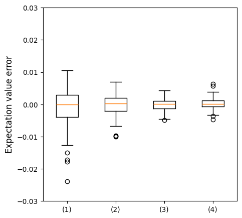
In order to validate our formula, we perform numerical simulations. We consider three and four partitions of an 8-qubit parametric circuit, where the partitions are created by cutting three and four gates, respectively (Figure 2). Note that the gate is identical to the CX gate up to local operations. By randomly choosing parameters in the circuit, we execute 100 different circuits and compute the expectation value of Pauli . For each circuit, the difference between the exact solution and the solution obtained from the circuit cutting algorithm [2] is computed as the expectation value error, and the distributions of these errors are plotted as boxplots (Figure 3). In this figure, (1) and (3) correspond to the results from the three partitions case, and (2) and (4) correspond to those from the four partitions case. The sampling numbers estimated for are used in cases (1) and (2), and those for are used in cases (3) and (4). The observed standard deviations are (1) , (2) , (3) , and (4) , which are smaller than for (1) and (2) and for (3) and (4), as expected. The sampling numbers estimated using our bound in eq. 9 and employed in the analysis are (1) , (2) , (3) , and (4) . These numbers may be compared with the estimations obtained by using eq. 7, (1) , (2) , (3) , and (4) . The discrepancy is particularly large in the cases of four partitions, i.e. (2) and (4). Nevertheless, the numerical results of (2) and (4) fall within the specified standard deviations, supporting the validity of our sampling number estimations using eq. 9. The numerical simulation was performed using Amazon Braket Python SDK [51] version 1.88.3.
3 Partitioning method
In this section, we detail our partitioning method and its implementation. Our method first converts a quantum circuit into an undirected graph with nodes and edges in such a way that each cluster of nodes corresponds to each partition of the circuit. This is detailed in sec. 3.1. The subsequent clustering has two steps. The first step is the modularity maximization clustering step. In this step, clusters are merged to increase modularity. The resulting clusters are further merged in the second step. These steps are detailed in secs. 3.2 and 3.3, respectively.
3.1 Doubly weighted graph

We convert a quantum circuit into an weighted graph with nodes , edges and two weight functions , where each function assigns a weight to each edge. Assume that we start with an input quantum circuit with 1- or 2-qubit gates. 1-qubit gates are ignored. First, a 2-qubit gate contributes to two nodes at the points where it interacts with the two qubit lines, and one edge between these two nodes. Cutting this edge corresponds to a space-like cut. Then, adjacent nodes on a common qubit line are connected with an edge, cutting which corresponds to a time-like cut. By performing node clustering on a graph defined in this way through edge cuts, we can achieve circuit partitioning using a combination of space-like and time-like cuts [31], where one cluster corresponds to one partition of the input circuit (see Figure 4).
As shown in eq. 9b, the sampling overhead can be different for each cluster. Based on eq. 9b, we define
| (13) |
where is the set of edges connecting nodes in the cluster to nodes in other clusters, and is the set of edges connecting nodes in clusters other than the cluster . Focusing on the largest overhead among the clusters, we define the following quantity as our objective function to minimize and as our metric for evaluating the quality of partitioning solutions,
| (14a) | ||||
| (14b) | ||||
where is the set of clusters. Since the overhead for each cluster can differ by orders of magnitude, focusing only on the maximum value is a reasonable approach. Moreover, we define
| (15a) | ||||
| (15b) | ||||
can be a dominant contribution to , therefore it is particularly important to partition the circuit so as to minimize .
We define the weight functions and for edge as
| (16a) | ||||
| (16b) | ||||
Namely, each edge carries the two types of weights at the same time. By defining weights in this way, computing and is as straightforward as counting the number of cut edges or computing the cluster degrees, as done in refs. [25, 27]. Throughout the following discussion, the term ”weight” primarily refers to the weight defined by eq. 16a.
3.2 Qubit-constrained modularity clustering step
The first step of node clustering on our weighted graphs is modularity maximization [52], where clusters are subsequently merged to increase modularity defined as [53, 52]
| (17a) | ||||
| (17b) | ||||
where is the sum of the weights of all the edges, , is the sum of the weights of edges connecting nodes within the cluster (each edge is counted only once), and is the sum of the weights of the edges attached to nodes within the cluster (double counting is possible if both endpoints of an edge belong to the same cluster). It is straightforward to confirm that
| (18a) | ||||
| (18b) | ||||
where eq. 16a is used at the last equal. Modularity maximization clusters nodes in a graph in such a way that increases the first term and decreases the second term in eq. 17a. Since eq. 18b shows that the second term in eq. 17a includes , modularity maximization with our weight definition in eq. 16 can reduce , which can be the dominant contribution to our objective function (see eqs. 15 14). This observation is one of our motivations to adopt modularity maximization. Another motivation is that there exists a simple heuristic algorithm that is known to quickly produce high-quality solutions [54]. Our algorithm of modularity maximization is based on ref. [54] and its implementation is influenced by refs. [55, 56].
Our weighted graph and the maximum number of qubits in devices, , are inputs to our algorithm. First, we assign each node to its own cluster , resulting in clusters. Then, we pick a node . Next, we select a cluster where is a set of clusters containing nodes connected to the node via edges. Assuming that the node is moved from to , we calculate the resulting number of qubits in . If that number is less than or equal to , we calculate the gain of modularity by moving from to . This calculation is performed for all the other . The node is actually moved to that yields the maximum gain. If the maximum gain is zero or negative, the node remains in . This operation is repeated for all the other . The above is repeated as long as node movements occur. This constitutes the first phase.
In the second phase, a new weighted graph is generated by contracting the clusters obtained in the first phase (each containing at least one node) into supernodes. The sum of the weights of all edges connecting two clusters becomes the weight of the new edge connecting the corresponding two supernodes. The sum of the weights of edges connecting nodes within a cluster is retained as the weight of the self-loop edge of the corresponding supernode.
The new weighted graph will be used as the input to the upcoming first phase. These two phases together are referred to as a ”pass”. This pass is repeated as long as node movements (i.e. increases in modularity) occur during the first phase. Note that there is arbitrariness in the order of selecting node in the first phase. In our numerical studies, we take the descending order of the sum of the weights of the edges connected to node . However, since our method is very fast as shown in Sec. 4, it is an option to run the random-order approach multiple times and select the best outcome in terms of .

The gain of modularity can be efficiently calculated from [54]
| (19) |
where is the gain of modularity by removing the node from the cluster :
| (20) |
and is the gain of modularity by adding the node to the cluster :
| (21) |
Here is the sum of the weights of edges connecting the node to nodes within the cluster , and is the sum of the weights of the edges attached to the node (including the self-loop edges). In Figure 5, we show an example of moving a node from its cluster to an adjacent cluster . For this simple example, we can easily find (refer to Figure 4 for the correspondence between the graph and the quantum circuit, and to Table 1 for the weights of edges)
| (22) |
By inputting these values into eqs. 19 20 21, the gain of modularity can be calculated using only the information from the cluster and as
| (23) |
where denotes the sum of the weights of all the edges and is a constant during the algorithm. We show the flow of the algorithm in Algorithm 1.
The use of modularity maximization for identifying cutting locations has already been validated in ref. [40]. However, ref. [40] considers only time-like cutting. In our method, by considering space-like cutting as well as time-like cutting, the size of a graph becomes twice as large as that in ref. [40] in terms of the number of nodes. The scalability of modularity maximization with respect to graph size demonstrates its strength when dealing with such large-scale graphs.
3.3 minimization clustering step
The modularity maximization algorithm [54] adopted in the first step is primarily intended to perform community detection, rather than to directly minimize our objective function in eq. 14 (although it is expected to contribute to reduction of it via reduction of as shown below eq. 18b). Therefore, the second step takes the result of the first step as input and further merges clusters. The merging is performed so as to reduce the value of .
The algorithm proceeds in almost the same manner as the first step. It consists of two phases, with the second phase being exactly the same. A ”pass”, which is the combination of two phases, is repeated in the same way. Differences lie in the first phase. At the beginning of each pass, the metric is computed. First, a node is picked up in the same way as the first step. Assuming that the node is removed from , the resulting in eq. 13 is calculated for . If this value is less than or equal to , we proceed to select a cluster and compute the resulting for assuming that the node is added to . Furthermore, we compute the change in the sum of the weights of all inter-cluster edges resulting from moving the node from to (denoted by ). If , or if and , then the node is moved to , and is updated to . In all the other cases, the node remains in . Naturally, it is also required that the number of qubits resulting from adding the node to does not exceed . This process is applied repeatedly and subsequently for all other clusters and nodes , as long as node movements occur. We show the flow of the algorithm in Algorithm 2.
One of the advantages of our method, which consists of step 1 and step 2, is that the optimal number of partitions is also automatically determined during the optimization process. In contrast, in many of graph partitioning algorithms such as mixed-integer programming (MIP) models, the number of partitions must be specified as input. For example, in ref. [27], which adopts a MIP model, their solver is run for all possible partition numbers from 2 to for a -qubit circuit in order to determine the optimal number of partitions. This approach may become computationally expensive for circuits with a large number of qubits.
4 Application to the QASMBench
| circuit | Time[sec] | |||||||
|---|---|---|---|---|---|---|---|---|
| Step 1 | Step 2 | Step 1 | Step 2 | Step 1 | Step 2 | Step 1 | Step 2 | |
| ising _ n34 _ D30 | 17.33 | 3.47 | 5.55 | 2.77 | 16 | 2 | 0.0025 | 0.0005 |
| ising _ n66 _ D30 | 18.08 | 6.64 | 5.55 | 5.55 | 17 | 3 | 0.0051 | 0.0007 |
| ising _ n66 _ D50 | 18.08 | 3.47 | 5.55 | 2.77 | 17 | 2 | 0.0056 | 0.0009 |
| ising _ n98 _ D30 | 23.28 | 7.62 | 5.55 | 5.55 | 24 | 4 | 0.0080 | 0.0014 |
| ising _ n98 _ D50 | 23.28 | 6.64 | 5.55 | 5.55 | 24 | 3 | 0.0080 | 0.0010 |
| ising _ n98 _ D70 | 23.28 | 3.47 | 5.55 | 2.77 | 24 | 2 | 0.0080 | 0.0008 |
| ising _ n420 _ D30 | 43.46 | 18.83 | 5.55 | 5.55 | 52 | 18 | 0.0887 | 0.0131 |
| ising _ n420 _ D50 | 43.46 | 11.90 | 5.55 | 5.55 | 52 | 9 | 0.0342 | 0.0072 |
| ising _ n420 _ D70 | 43.46 | 10.26 | 5.55 | 5.55 | 52 | 7 | 0.0340 | 0.0057 |
_
_
In order to verify the validity of our method, we apply it on a number of benchmark quantum circuits and compare the results with those obtained using find_cuts function from Qiskit-addon-cutting (QAC) [48] version 0.10.0, which is a representative tool that integrates the functions required for circuit cutting. As benchmark quantum circuits, we adopt the circuits from the large-scale category of QASMBench [49]. Only circuits in which all entangling gates have been transpiled into CX gates, as given by xxx_transpiled.qasm, are adopted. However, circuits containing mid-circuit measurements (e.g., cc_nyyy_transpiled.qasm) and those that are excessively large (e.g., bwt_nyyy_transpiled.qasm) are excluded.
To first verify that our algorithm behaves as intended, we compare the outputs of the first step with those of the second step which takes the output of the first step as its input. Using the Ising circuits from QASMBench as an example, we measure the metric in eq. 14, in eq. 15, the number of partitions , and the execution time (see Table 2). We can observe that the value of is nearly minimized in the first step, and in some cases, no further reduction is observed in the second step. This may be expected from the property of modularity maximization as explained below eq. 18. In the second step, is meaningfully reduced while is preserved or reduced. This indicates that the second step reduces and minimizes the contributions other than . It is also found that, when is large, is not necessarily the dominant contribution to . The execution time is generally quite fast. In particular, the second step tends to be faster than the first step, as it starts with a smaller number of initial clusters.
For a larger set of circuits (83 in total) from QASMBench, we compare the results of this work’s algorithm (TWA) with those of QAC. Let us define () as the number of space-like (time-like) edges in . Since all entangling gates in the circuits are already transpiled into CX gates, in eq. 15 can be expressed as
| (24) |
We also introduce , the total number of space-like cuts, and , the total number of space-like cuts, and define
| (25) |
Note that QAC partitions the circuit with the objective of minimizing the quantity corresponding to .
The two approaches are compared in terms of , , , , and the execution time (see Table LABEL:tbl:all). Regarding , we can observe that the results of TWA are equal to or smaller (i.e. better) than those of QAC in all but 6 out of the 83 circuits. As for , TWA performs worse than QAC only in 6 circuits. Furthermore, QAC encountered overflow errors in a number of the circuits, which are denoted by -|-. It is noteworthy that, although the quantity corresponding to is the objective function of QAC, TWA still achieves the better results with respect to on average. With respect to execution time, TWA significantly outperforms QAC by achieving a speedup ranging from to depending on the circuit with an average speedup of .
_
_
| circuit | Time[sec] | |||||||||
|---|---|---|---|---|---|---|---|---|---|---|
| TWA | QAC | TWA | QAC | TWA | QAC | TWA | QAC | TWA | QAC | |
|
adder
_ _ |
5.5 | 5.5 | 2/0 | 2/0 | 4.4 | 4.4 | 3 | 3 | 0.04 | 0.80 |
|
adder
_ _ |
2.9 | 2.9 | 1/0 | 1/0 | 2.2 | 2.2 | 2 | 2 | 0.03 | 0.05 |
|
adder
_ _ |
6.8 | 54 | 2/0 | 22/0 | 8.8 | 72 | 5 | 4 | 0.06 | 50.9 |
|
adder
_ _ |
5.5 | 5.5 | 2/0 | 2/0 | 4.4 | 4.4 | 3 | 3 | 0.06 | 2.15 |
|
adder
_ _ |
2.9 | 2.9 | 1/0 | 1/0 | 2.2 | 2.2 | 2 | 2 | 0.06 | 0.10 |
|
adder
_ _ |
12 | 104 | 2/0 | 22/0 | 32 | 338 | 16 | 15 | 0.24 | 74.6 |
|
adder
_ _ |
9.5 | 77 | 2/0 | 22/0 | 19 | 193 | 10 | 9 | 0.29 | 87.7 |
|
adder
_ _ |
8.0 | 68 | 2/0 | 22/0 | 13 | 145 | 7 | 7 | 0.23 | 85.6 |
|
bv
_ _ |
3.5 | 6.3 | 0/1 | 0/1 | 2.8 | 2.8 | 2 | 0.04 | ||
|
bv
_ _ |
6.6 | 9.8 | 0/2 | 0/2 | 5.5 | 5.5 | 3 | 2.54 | ||
|
bv
_ _ |
3.5 | 7.0 | 0/1 | 0/1 | 2.8 | 2.8 | 2 | 0.09 | ||
|
bv
_ _ |
3.5 | 7.0 | 0/1 | 0/1 | 2.8 | 2.8 | 2 | 0.16 | ||
|
bv
_ _ |
10 | 275 | 0/2 | 123/0 | 16 | 270 | 7 | 251 | 0.01 | 9.54 |
|
bv
_ _ |
7.6 | 231 | 0/2 | 103/0 | 8.3 | 226 | 4 | 231 | 0.01 | 22.0 |
|
bv
_ _ |
6.6 | 187 | 0/2 | 83/0 | 5.5 | 182 | 3 | 211 | 0.01 | 22.2 |
|
cat
_ _ |
5.5 | 5.5 | 2/0 | 2/0 | 4.4 | 4.4 | 3 | 3 | 0.11 | |
|
cat
_ _ |
2.9 | 2.9 | 1/0 | 1/0 | 2.2 | 2.2 | 2 | 2 | 0.01 | |
|
cat
_ _ |
6.8 | 6.8 | 2/0 | 2/0 | 8.8 | 8.8 | 5 | 5 | 0.01 | 16.4 |
|
cat
_ _ |
5.5 | 5.5 | 2/0 | 2/0 | 4.4 | 4.4 | 3 | 3 | 0.01 | 0.31 |
|
cat
_ _ |
2.9 | 2.9 | 1/0 | 1/0 | 2.2 | 2.2 | 2 | 2 | 0.01 | 0.01 |
|
cat
_ _ |
10 | 9.0 | 2/0 | 2/0 | 21 | 17 | 11 | 9 | 0.02 | 20.6 |
|
cat
_ _ |
7.4 | 7.4 | 2/0 | 2/0 | 10 | 10 | 6 | 6 | 0.01 | 33.9 |
|
cat
_ _ |
6.2 | 6.2 | 2/0 | 2/0 | 6.6 | 6.6 | 4 | 4 | 0.01 | 32.4 |
|
ghz
_ _ |
5.5 | 5.5 | 2/0 | 2/0 | 4.4 | 4.4 | 3 | 3 | 0.11 | |
|
ghz
_ _ |
2.9 | 2.9 | 1/0 | 1/0 | 2.2 | 2.2 | 2 | 2 | 0.01 | |
|
ghz
_ _ |
2.9 | 2.9 | 1/0 | 1/0 | 2.2 | 2.2 | 2 | 2 | 0.01 | |
|
ghz
_ _ |
6.8 | 6.8 | 2/0 | 2/0 | 8.8 | 8.8 | 5 | 5 | 0.01 | 16.6 |
|
ghz
_ _ |
5.5 | 5.5 | 2/0 | 2/0 | 4.4 | 4.4 | 3 | 3 | 0.01 | 0.30 |
|
ghz
_ _ |
2.9 | 2.9 | 1/0 | 1/0 | 2.2 | 2.2 | 2 | 2 | 0.01 | 0.01 |
|
ghz
_ _ |
10 | 9.0 | 2/0 | 2/0 | 21 | 17 | 11 | 9 | 0.01 | 19.9 |
|
ghz
_ _ |
7.4 | 7.4 | 2/0 | 2/0 | 10 | 10 | 6 | 6 | 0.01 | 33.6 |
|
ghz
_ _ |
6.2 | 6.2 | 2/0 | 2/0 | 6.6 | 6.6 | 4 | 4 | 0.01 | 32.2 |
|
ising
_ _ |
6.6 | 6.6 | 0/2 | 0/2 | 5.5 | 5.5 | 3 | 3 | 0.01 | 0.39 |
|
ising
_ _ |
3.5 | 3.5 | 0/1 | 0/1 | 2.8 | 2.8 | 2 | 2 | 0.01 | 0.02 |
|
ising
_ _ |
7.6 | 10 | 0/2 | 4/0 | 8.3 | 13 | 4 | 4 | 0.01 | 16.1 |
|
ising
_ _ |
6.6 | 3.5 | 0/2 | 0/1 | 5.5 | 2.8 | 3 | 2 | 0.01 | 0.03 |
|
ising
_ _ |
3.5 | 3.5 | 0/1 | 0/1 | 2.8 | 2.8 | 2 | 2 | 0.01 | 0.03 |
|
ising
_ _ |
18 | 20 | 0/2 | 4/0 | 47 | 57 | 18 | 14 | 0.05 | 17.9 |
|
ising
_ _ |
11 | 15 | 0/2 | 4/0 | 22 | 35 | 9 | 9 | 0.05 | 27.3 |
|
ising
_ _ |
10 | 13 | 0/2 | 4/0 | 16 | 21 | 7 | 6 | 0.05 | 13.7 |
|
knn
_ _ |
6.6 | 6.6 | 0/2 | 0/2 | 5.5 | 5.5 | 3 | 3 | 0.01 | 0.45 |
|
knn
_ _ |
3.5 | 3.5 | 0/1 | 0/1 | 2.8 | 2.8 | 2 | 2 | 0.01 | 0.04 |
|
knn
_ _ |
8.5 | 443 | 0/2 | 200/0 | 11 | 439 | 5 | 51 | 0.03 | 6.58 |
|
knn
_ _ |
6.6 | 6.6 | 0/2 | 0/2 | 5.5 | 5.5 | 3 | 3 | 0.03 | 1.37 |
|
knn
_ _ |
3.5 | 3.5 | 0/1 | 0/1 | 2.8 | 2.8 | 2 | 2 | 0.03 | 0.08 |
|
knn
_ _ |
15 | 1376 | 0/2 | 624/0 | 36 | 1371 | 14 | 157 | 0.08 | 7.53 |
|
knn
_ _ |
11 | 1288 | 0/2 | 584/0 | 19 | 1283 | 8 | 147 | 0.12 | 26.6 |
|
knn
_ _ |
9.4 | 1200 | 0/2 | 544/0 | 13 | 1195 | 6 | 137 | 0.07 | 30.6 |
|
qft
_ _ |
318 | -|- | 0/60 | -|- | 765 | -|- | 13 | -|- | 0.26 | -|- |
|
qft
_ _ |
246 | -|- | 0/81 | -|- | 307 | -|- | 4 | -|- | 0.27 | -|- |
|
qft
_ _ |
1020 | -|- | 0/70 | -|- | 3482 | -|- | 52 | -|- | 1.02 | -|- |
|
qft
_ _ |
643 | -|- | 0/102 | -|- | 1713 | -|- | 17 | -|- | 2.94 | -|- |
|
qft
_ _ |
481 | -|- | 0/96 | -|- | 1120 | -|- | 10 | -|- | 1.33 | -|- |
|
qft
_ _ |
2120 | -|- | 0/70 | -|- | 7879 | -|- | 115 | -|- | 2.80 | -|- |
|
qft
_ _ |
1169 | -|- | 0/116 | -|- | 3698 | -|- | 36 | -|- | 3.14 | -|- |
|
qft
_ _ |
704 | -|- | 0/102 | -|- | 1960 | -|- | 16 | -|- | 3.10 | -|- |
|
qugan
_ _ |
32 | 448 | 0/6 | 202/0 | 72 | 461 | 9 | 3 | 0.03 | 13.7 |
|
qugan
_ _ |
9.0 | 286 | 0/3 | 130/0 | 8.3 | 285 | 2 | 2 | 0.22 | 30.8 |
|
qugan
_ _ |
9.0 | 22 | 0/3 | 10/0 | 8.3 | 21 | 2 | 2 | 0.04 | 26.5 |
|
qugan
_ _ |
22 | 659 | 0/6 | 282/0 | 33 | 830 | 5 | 4 | 0.05 | 14.7 |
|
qugan
_ _ |
17 | 711 | 0/6 | 322/0 | 16 | 725 | 3 | 3 | 0.05 | 50.7 |
|
qugan
_ _ |
9.0 | 549 | 0/3 | 250/0 | 8.3 | 549 | 2 | 2 | 0.10 | 15.4 |
|
qugan
_ _ |
48 | -|- | 0/6 | -|- | 133 | -|- | 17 | -|- | 0.23 | -|- |
|
qugan
_ _ |
33 | -|- | 0/6 | -|- | 74 | -|- | 10 | -|- | 0.24 | -|- |
|
qugan
_ _ |
26 | -|- | 0/6 | -|- | 49 | -|- | 7 | -|- | 0.23 | -|- |
|
swap
_ _ _ |
6.6 | 6.6 | 0/2 | 0/2 | 5.5 | 5.5 | 3 | 3 | 0.02 | 0.39 |
|
swap
_ _ _ |
3.5 | 3.5 | 0/1 | 0/1 | 2.8 | 2.8 | 2 | 2 | 0.02 | 0.05 |
|
swap
_ _ _ |
3.5 | 3.5 | 0/1 | 0/1 | 2.8 | 2.8 | 2 | 2 | 0.02 | 0.05 |
|
swap
_ _ _ |
8.5 | 381 | 0/2 | 172/0 | 11 | 377 | 5 | 44 | 0.02 | 6.66 |
|
swap
_ _ _ |
6.6 | 6.6 | 0/2 | 0/2 | 5.5 | 5.5 | 3 | 3 | 0.02 | 1.26 |
|
swap
_ _ _ |
3.5 | 3.5 | 0/1 | 0/1 | 2.8 | 2.8 | 2 | 2 | 0.02 | 0.07 |
|
swap
_ _ _ |
16 | -|- | 0/2 | -|- | 38 | -|- | 15 | -|- | 0.09 | -|- |
|
swap
_ _ _ |
11 | 1376 | 0/2 | 624/0 | 19 | 1371 | 8 | 157 | 0.07 | 28.2 |
|
swap
_ _ _ |
9.4 | 1288 | 0/2 | 584/0 | 13 | 1283 | 6 | 147 | 0.08 | 31.6 |
|
wstate
_ _ |
9.9 | 9.9 | 4/0 | 4/0 | 8.8 | 8.8 | 3 | 3 | 0.01 | 14.5 |
|
wstate
_ _ |
5.1 | 5.1 | 2/0 | 2/0 | 4.4 | 4.4 | 2 | 2 | 0.01 | 0.34 |
|
wstate
_ _ |
5.1 | 5.1 | 2/0 | 2/0 | 4.4 | 4.4 | 2 | 2 | 0.01 | 0.55 |
|
wstate
_ _ |
12 | 10 | 4/0 | 4/0 | 17 | 13 | 5 | 4 | 0.01 | 21.0 |
|
wstate
_ _ |
9.9 | 9.9 | 4/0 | 4/0 | 8.8 | 8.8 | 3 | 3 | 0.01 | 31.2 |
|
wstate
_ _ |
5.1 | 5.1 | 2/0 | 2/0 | 4.4 | 4.4 | 2 | 2 | 0.01 | 0.67 |
|
wstate
_ _ |
28 | 19 | 4/0 | 4/0 | 96 | 52 | 23 | 13 | 0.04 | 20.8 |
|
wstate
_ _ |
15 | 14 | 4/0 | 4/0 | 35 | 30 | 9 | 8 | 0.04 | 36.7 |
|
wstate
_ _ |
13 | 13 | 4/0 | 4/0 | 21 | 21 | 6 | 6 | 0.04 | 50.2 |
5 Conclusion and discussion
We have introduced a novel method for identifying cut locations for quantum circuit cutting, with a primary focus on partitioning large circuits into three or more parts. Under the assumption that the classical postprocessing function is decomposable, we have first derived the upper bound on the sampling overhead. We have shown that this new bound significantly improves upon the previously known bound, which is based on the total number of cuts, by orders of magnitude in cases of three or more partitions. The validity of our bound has been confirmed through the numerical simulations on circuits partitioned into three and four parts.
Next, based on the newly derived upper bound on the sampling overhead, we have defined a new objective function and proposed a method to identify cutting locations that minimize it. This objective function more appropriately reflects the sampling overhead in solutions of three or more partitions, compared to the total number of cuts used in the previous methods. To validate our method, we applied it to 83 quantum circuits from the large scale category of QASMBench. We used the results obtained from Qiskit-addon-cutting (QAC) as the baseline. We have observed that our method significantly outperforms QAC in terms of computation time by achieving a speedup ranging from to depending on the circuit with an average speedup of . In terms of solution quality with respect to , our method has performed comparable to or better than QAC in all but 6 out of the 83 circuits.
In our derivation of the upper bound on the sampling overhead, we assume independent cutting approaches [1, 2, 19]. Accordingly, the baseline for comparison (eq. 7) is also based on this assumption. It has been shown that the sampling overhead can be reduced using techniques such as joint cutting and parallel cutting; see e.g. refs. [11, 20, 12, 21]. Since these studies focus on bipartitions, extending joint cutting and/or parallel cutting to cases of more than two partitions may be a promising direction for future research.
Acknowledgments
The views expressed in this research are those of the authors and do not necessarily reflect the official policy or position of PwC Consulting LLC. We wish to thank Mitsuhiro Matsumoto, Tsuyoshi Kitano, Hana Ebi, Hideaki Kawaguchi, Hiroki Kuji, Shigetora Miyashita, Shin Nishio and Takaharu Yoshida for stimulating discussion and support. This work is supported by New Energy and Industrial Technology Development Organization (NEDO).
References
- [1] Tianyi Peng, Aram W. Harrow, Maris Ozols, and Xiaodi Wu. Simulating large quantum circuits on a small quantum computer. Physical Review Letters, 125(15), oct 2020.
- [2] Kosuke Mitarai and Keisuke Fujii. Constructing a virtual two-qubit gate by sampling single-qubit operations. New Journal of Physics, 23(2):023021, feb 2021.
- [3] Thomas Ayral, Francois-Marie Le Regent, Zain Saleem, Yuri Alexeev, and Martin Suchara. Quantum divide and compute: Hardware demonstrations and noisy simulations. In 2020 IEEE Computer Society Annual Symposium on VLSI (ISVLSI), page 138–140. IEEE, July 2020.
- [4] Thomas Ayral, François-Marie Le Régent, Zain Saleem, Yuri Alexeev, and Martin Suchara. Quantum divide and compute: Exploring the effect of different noise sources. SN Computer Science, 2(3), March 2021.
- [5] Chong Ying, Bin Cheng, Youwei Zhao, He-Liang Huang, Yu-Ning Zhang, Ming Gong, Yulin Wu, Shiyu Wang, Futian Liang, Jin Lin, et al. Experimental simulation of larger quantum circuits with fewer superconducting qubits. Physical review letters, 130(11):110601, 2023.
- [6] Takahiro Yamamoto and Ryutaro Ohira. Error suppression by a virtual two-qubit gate. Journal of Applied Physics, 133(17), May 2023.
- [7] Marvin Bechtold, Johanna Barzen, Frank Leymann, Alexander Mandl, Julian Obst, Felix Truger, and Benjamin Weder. Investigating the effect of circuit cutting in qaoa for the maxcut problem on nisq devices. Quantum Science and Technology, 8(4):045022, 2023.
- [8] Almudena Carrera Vazquez, Caroline Tornow, Diego Ristè, Stefan Woerner, Maika Takita, and Daniel J. Egger. Combining quantum processors with real-time classical communication. Nature, 636(8041):75–79, November 2024.
- [9] Akhil Pratap Singh, Kosuke Mitarai, Yasunari Suzuki, Kentaro Heya, Yutaka Tabuchi, Keisuke Fujii, and Yasunobu Nakamura. Experimental demonstration of a high-fidelity virtual two-qubit gate. Physical Review Research, 6(1):013235, 2024.
- [10] Akhil Pratap Singh, Kenji Sugisaki, Srinivasa Prasannaa, Bijaya Kumar Sahoo, Bhanu Pratap Das, and Yasunobu Nakamura. Experimental computations of atomic properties on a superconducting quantum processor. Phys. Rev. A, 110:062620, Dec 2024.
- [11] Angus Lowe, Matija Medvidović, Anthony Hayes, Lee J. O’Riordan, Thomas R. Bromley, Juan Miguel Arrazola, and Nathan Killoran. Fast quantum circuit cutting with randomized measurements. Quantum, 7:934, 2023.
- [12] Hiroyuki Harada, Kaito Wada, and Naoki Yamamoto. Doubly optimal parallel wire cutting without ancilla qubits. PRX Quantum, 5(4):040308, 2024.
- [13] Edwin Pednault. An alternative approach to optimal wire cutting without ancilla qubits, 2023.
- [14] Lukas Brenner, Christophe Piveteau, and David Sutter. Optimal wire cutting with classical communication, 2023.
- [15] Aram W. Harrow and Angus Lowe. Optimal quantum circuit cuts with application to clustered hamiltonian simulation. PRX Quantum, 6(1), January 2025.
- [16] Marvin Bechtold, Johanna Barzen, Frank Leymann, and Alexander Mandl. Circuit cutting with non-maximally entangled states, 2023.
- [17] Marvin Bechtold, Johanna Barzen, Frank Leymann, and Alexander Mandl. Cutting a wire with non-maximally entangled states. In 2024 IEEE International Parallel and Distributed Processing Symposium Workshops (IPDPSW), page 1136–1145. IEEE, May 2024.
- [18] Marvin Bechtold, Johanna Barzen, Frank Leymann, Alexander Mandl, and Felix Truger. Joint wire cutting with non‐maximally entangled states. Advanced Quantum Technologies, 8(5), January 2025.
- [19] Kosuke Mitarai and Keisuke Fujii. Overhead for simulating a non-local channel with local channels by quasiprobability sampling. Quantum, 5:388, 2021.
- [20] Christophe Piveteau and David Sutter. Circuit knitting with classical communication. IEEE Transactions on Information Theory, 70(4):2734–2745, April 2024.
- [21] Christian Ufrecht, Maniraman Periyasamy, Sebastian Rietsch, Daniel D. Scherer, Axel Plinge, and Christopher Mutschler. Cutting multi-control quantum gates with zx calculus. Quantum, 7:1147, October 2023.
- [22] Christian Ufrecht, Laura S Herzog, Daniel D Scherer, Maniraman Periyasamy, Sebastian Rietsch, Axel Plinge, and Christopher Mutschler. Optimal joint cutting of two-qubit rotation gates. Physical Review A, 109(5):052440, 2024.
- [23] Lukas Schmitt, Christophe Piveteau, and David Sutter. Cutting circuits with multiple two-qubit unitaries. Quantum, 9:1634, 2025.
- [24] Marco Schumann, Tobias Stollenwerk, and Alessandro Ciani. Bridging wire and gate cutting with zx-calculus, 2025.
- [25] Wei Tang, Teague Tomesh, Martin Suchara, Jeffrey Larson, and Margaret Martonosi. Cutqc: using small quantum computers for large quantum circuit evaluations. In Proceedings of the 26th ACM International conference on architectural support for programming languages and operating systems, pages 473–486, 2021.
- [26] Michael A. Perlin, Zain H. Saleem, Martin Suchara, and James C. Osborn. Quantum circuit cutting with maximum-likelihood tomography. npj Quantum Information, 7(1), April 2021.
- [27] Wei Tang and Margaret Martonosi. Scaleqc: A scalable framework for hybrid computation on quantum and classical processors. arXiv preprint arXiv:2207.00933, 2022.
- [28] Ryo Nagai, Shu Kanno, Yuki Sato, and Naoki Yamamoto. Quantum channel decomposition with preselection and postselection. Phys. Rev. A, 108:022615, Aug 2023.
- [29] Gian Gentinetta, Friederike Metz, and Giuseppe Carleo. Overhead-constrained circuit knitting for variational quantum dynamics. Quantum, 8:1296, March 2024.
- [30] Gideon Uchehara, Tor M. Aamodt, and Olivia Di Matteo. Rotation-inspired circuit cut optimization, 2022.
- [31] Sebastian Brandhofer, Ilia Polian, and Kevin Krsulich. Optimal partitioning of quantum circuits using gate cuts and wire cuts. IEEE Transactions on Quantum Engineering, 2023.
- [32] Turbasu Chatterjee, Arnav Das, Shah Ishmam Mohtashim, Amit Saha, and Amlan Chakrabarti. Qurzon: A prototype for a divide and conquer-based quantum compiler for distributed quantum systems. SN Computer Science, 3(4):323, 2022.
- [33] Hang Lian, Jinchen Xu, Yu Zhu, Zhiqiang Fan, Yi Liu, and Zheng Shan. Fast reconstruction algorithm based on hmc sampling. Scientific Reports, 13(1):17773, 2023.
- [34] Debasmita Bhoumik, Ritajit Majumdar, Amit Saha, and Susmita Sur-Kolay. Distributed scheduling of quantum circuits with noise and time optimization. arXiv preprint arXiv:2309.06005, 2023.
- [35] Martin Beisel, Johanna Barzen, Marvin Bechtold, Frank Leymann, Felix Truger, Benjamin Weder, et al. Quantme4vqa: Modeling and executing variational quantum algorithms using workflows. In CLOSER, pages 306–315, 2023.
- [36] Daniel T. Chen, Ethan H. Hansen, Xinpeng Li, Vinooth Kulkarni, Vipin Chaudhary, Bin Ren, Qiang Guan, Sanmukh Kuppannagari, Ji Liu, and Shuai Xu. Efficient Quantum Circuit Cutting by Neglecting Basis Elements . In 2023 IEEE International Parallel and Distributed Processing Symposium Workshops (IPDPSW), pages 517–523, Los Alamitos, CA, USA, May 2023. IEEE Computer Society.
- [37] Xinpeng Li, Vinooth Kulkarni, Daniel T. Chen, Qiang Guan, Weiwen Jiang, Ning Xie, Shuai Xu, and Vipin Chaudhary. Efficient circuit wire cutting based on commuting groups, 2024.
- [38] Aditya Pawar, Yingheng Li, Zewei Mo, Yanan Guo, Xulong Tang, Youtao Zhang, and Jun Yang. Qrcc: Evaluating large quantum circuits on small quantum computers through integrated qubit reuse and circuit cutting. In Proceedings of the 29th ACM International Conference on Architectural Support for Programming Languages and Operating Systems, Volume 4, ASPLOS ’24, page 236–251. ACM, April 2024.
- [39] Philipp Seitz, Manuel Geiger, and Christian B. Mendl. Multithreaded parallelism for heterogeneous clusters of qpus. In ISC High Performance 2024 Research Paper Proceedings (39th International Conference), page 1–8. IEEE, May 2024.
- [40] Shuwen Kan, Zefan Du, Miguel Palma, Samuel A Stein, Chenxu Liu, Wenqi Wei, Juntao Chen, Ang Li, and Ying Mao. Scalable circuit cutting and scheduling in a resource-constrained and distributed quantum system. arXiv preprint arXiv:2405.04514, 2024.
- [41] Xiangyu Ren, Mengyu Zhang, and Antonio Barbalace. A hardware-aware gate cutting framework for practical quantum circuit knitting. In Proceedings of the 43rd IEEE/ACM International Conference on Computer-Aided Design, ICCAD ’24, page 1–9. ACM, October 2024.
- [42] Xinglei Dou, Lei Liu, Zhuohao Wang, and Pengyu Li. Larqucut: A new cutting and mapping approach for large-sized quantum circuits in distributed quantum computing (dqc) environments, 2025.
- [43] Ritajit Majumdar and Christopher J. Wood. Error mitigated quantum circuit cutting, 2022.
- [44] Nathaniel Tornow, Emmanouil Giortamis, and Pramod Bhatotia. Scaling quantum computations via gate virtualization, 2024.
- [45] Nathaniel Tornow, Christian B. Mendl, and Pramod Bhatotia. Quantum-classical computing via tensor networks, 2024.
- [46] Saikat Basu, Amit Saha, Amlan Chakrabarti, and Susmita Sur-Kolay. i -qer: An intelligent approach towards quantum error reduction. ACM Transactions on Quantum Computing, 3(4):1–18, July 2022.
- [47] Saikat Basu, Arnav Das, Amit Saha, Amlan Chakrabarti, and Susmita Sur-Kolay. Fragqc: An efficient quantum error reduction technique using quantum circuit fragmentation. Journal of Systems and Software, 214:112085, August 2024.
- [48] Agata M. Brańczyk, Almudena Carrera Vazquez, Daniel J. Egger, Bryce Fuller, Julien Gacon, James R. Garrison, Jennifer R. Glick, Caleb Johnson, Saasha Joshi, Edwin Pednault, C. D. Pemmaraju, Pedro Rivero, Ibrahim Shehzad, and Stefan Woerner. Qiskit addon: circuit cutting. https://github.com/Qiskit/qiskit-addon-cutting, 2024.
- [49] Ang Li, Samuel Stein, Sriram Krishnamoorthy, and James Ang. Qasmbench: A low-level quantum benchmark suite for nisq evaluation and simulation. ACM Transactions on Quantum Computing, 4(2):1–26, 2023.
- [50] Ali Javadi-Abhari, Matthew Treinish, Kevin Krsulich, Christopher J. Wood, Jake Lishman, Julien Gacon, Simon Martiel, Paul D. Nation, Lev S. Bishop, Andrew W. Cross, Blake R. Johnson, and Jay M. Gambetta. Quantum computing with Qiskit, 2024.
- [51] Amazon Web Services. Amazon braket sdk. https://github.com/amazon-braket/amazon-braket-sdk-python.
- [52] Aaron Clauset, M. E. J. Newman, and Cristopher Moore. Finding community structure in very large networks. Physical Review E, 70(6), December 2004.
- [53] Mark EJ Newman. Analysis of weighted networks. Physical Review E—Statistical, Nonlinear, and Soft Matter Physics, 70(5):056131, 2004.
- [54] Vincent D Blondel, Jean-Loup Guillaume, Renaud Lambiotte, and Etienne Lefebvre. Fast unfolding of communities in large networks. Journal of statistical mechanics: theory and experiment, 2008(10):P10008, 2008.
- [55] Aric A Hagberg, Daniel A Schult, and Pieter J Swart. Exploring network structure, dynamics, and function using networkx. In Proceedings of the 7th Python in Science Conference (SciPy2008), pages 11–15. Pasadena, CA USA, 2008.
- [56] NetworkX Developers. Networkx. https://github.com/networkx/networkx. Accessed: 2025-05-29.
Appendix A Derivation of sampling overhead for three or more partitions
Substituting eq. 4 into eq. 3 results in
| (26) |
where is the probability of obtaining provided the circuits specified by are run,
| (27) |
When the postprocess function is decomposed as eq. 8, the observable in eq. 1 can be manipulated as
| (28) |
Moreover, the expectation value in eq. 26 can be written as
| (29) |
To make the manipulation simpler, we will consider a specific case of and as illustrated in Figure 1. In this case, eq. 29 becomes
| (30) |
Let us define a random variable as
| (31) |
with the following random variables,
| (32a) | ||||
| (32b) | ||||
| (32c) | ||||
Since these random variables can be independently sampled as
| (33a) | ||||
| (33b) | ||||
| (33c) | ||||
we find
| (34) | ||||
| (35) |
where eq. 30 is referred. Below we show that the standard deviation of can be bounded by , namely
| (36) |
if the number of sampling for each partition satisfies
| (37a) | ||||
| (37b) | ||||
| (37c) | ||||
Within the partition , the number of samples will be used to run the circuit specified by ,
| (38a) | ||||
| Similarly, for partitions and , | ||||
| (38b) | ||||
| (38c) | ||||
The variance of , which is an each term in of eq. 31, can be calculated as
| (39) | ||||
| (40) |
where it is assumed that each variance is sufficiently controlled as in eq. 39. It is straightforward to show that
| (41) | ||||
| (42) | ||||
| (43) |
where eqs. 37, 38 are used. Generalizing the above argument to any and is straightforward. In particular, eq. 37 can be generalized to eq. 9.
Finally, we compare with the result presented in ref. [1]. Ref. [1] shows that the sampling overhead for three or more partitions via time-like cutting under the assumption of eq. 8 is upper-bounded by
| (44) |
where is the maximum number of time-like cuts on any partition. In the case of our example shown in Figure 1, this formula gives
| (45) |
which is much larger than our estimation in eq. 11. In ref. [1], the upper bound is derived using the Hoeffding’s inequality, whereas our approach differs in that we obtain it by computing the variance. Moreover, while the result in ref. [1] is based on the partition that requires the largest number of samples, our method provides the upper bound for each partition individually. Therefore, our result can be considered as an improvement on the upper bound proposed in ref. [1].
