跳到论文正文
W Papers独立论文阅读器 arXiv:2506.15915 论文正文 计算阅读时间 · 0%
引用这篇论文根据当前论文元数据生成,正式投稿前建议核对。


Estimating Multiple Weighted Networks with Node-Sparse Differences and Shared Low-Rank Structure

Hao Yan Department of Statistics, University of Wisconsin–Madison {hyan84,kdlevin}@wisc.edu Keith Levin Department of Statistics, University of Wisconsin–Madison {hyan84,kdlevin}@wisc.edu
Abstract

We study the problem of modeling multiple symmetric, weighted networks defined on a common set of nodes, where networks arise from different groups or conditions. We propose a model in which each network is expressed as the sum of a shared low-rank structure and a node-sparse matrix that captures the differences between conditions. This formulation is motivated by practical scenarios, such as in connectomics, where most nodes share a global connectivity structure while only a few exhibit condition-specific deviations. We develop a multi-stage estimation procedure that combines a spectral initialization step, semidefinite programming for support recovery, and a debiased refinement step for low-rank estimation. We establish minimax-optimal guarantees for recovering the shared low-rank component under the row-wise ℓ2,∞\ell_{2,\infty} norm and elementwise ℓ∞\ell_{\infty} norm, as well as for detecting node-level perturbations under various signal-to-noise regimes. We demonstrate that the availability of multiple networks can significantly enhance estimation accuracy compared to single-network settings. Additionally, we show that commonly-used methods such as group Lasso may provably fail to recover the sparse structure in this setting, a result which might be of independent interest.

1 Introduction

Networks are a fundamental data object in modern statistical applications, arising in domains as varied as neuroscience (Sporns, 2011; Bassett and Sporns, 2017; Guha et al., 2024), economics (Easley and Kleinberg, 2010; Diebold and Yılmaz, 2014) and social science (Granovetter, 1973; Borgatti et al., 2009), to name just a few. While modeling a single network has received extensive attention in recent decades— e.g., through Stochastic Block Models (SBM; Holland et al., 1983; Airoldi et al., 2008; Karrer and Newman, 2011), latent space models such as Hoff models Hoff et al., (2002), Random Dot Product Graphs (RDPG; Young and Scheinerman, 2007; Sussman et al., 2012; Athreya et al., 2018) and graphons (Lovász, 2012)— modeling multiple networks (also known as multilayer networks Kivelä et al., 2014) has recently been of growing interest to the network analysis community. In many practical scenarios, one observes multiple networks on a common set of nodes, with individual networks corresponding to different experimental conditions, populations, or time points. For example, functional magnetic resonance imaging (fMRI) data yield brain networks in which nodes represent brain regions. These regions can be consistently aligned across subjects, enabling comparisons of brain connectivity across different populations, disease statuses, ages, or cognitive tasks (Vaiana and Muldoon, 2020). Other examples include temporal gene co-expression networks (Bakken et al., 2016) and international food and agriculture trade networks (De Domenico et al., 2015). A central goal of inference in these settings is to identify both the structure that is shared across conditions and the systematic differences between them.

We briefly review recent developments in the statistical analysis of multiple networks. Levin et al., (2017) proposed the omnibus embedding method for jointly embedding multiple networks sharing a common low-rank mean structure. Subsequently, Levin et al., (2022) extended this framework to accommodate heterogeneous edge noise across graphs while maintaining a shared low-rank structure in expectation. Moving beyond shared mean structure, Lei and Lin, (2023) analyzed a multilayer SBM (MLSBM), where each network shares a common community structure but permits heterogeneous edge probabilities. Lei et al., (2024) further investigated the fundamental limits of community detection and parameter estimation in MLSBM. As an extension of the MLSBM, Nielsen and Witten, (2018) considered a model with multiple RDPGs sharing a common eigenspace. Building on this idea, Arroyo et al., (2021) assumed that the adjacency matrices share a common invariant subspace in expectation, and Xie, (2024) proposed a bias-corrected joint spectral embedding method tailored for this setting.

All of the above works assume a shared subspace structure underlying the edge probabilities. Relaxing this assumption, MacDonald et al., 2022b considered collections of networks following the generalized RDPG model (Rubin-Delanchy et al., 2022), under the assumption that the latent position matrix of each network is a concatenation of shared and individual latent position matrices. Several works have also explored incorporating auxiliary covariates into multilayer network models (e.g., MacDonald et al., 2022a ; Zhang et al., 2023). More broadly, various extensions of other models to the multilayer setting have been proposed; see, for example, Gollini and Murphy, (2016); Chen and Hero, (2017); Salter-Townshend and McCormick, (2017); D’Angelo et al., (2019); Sosa and Betancourt, (2022); He et al., (2023).

This paper addresses the problem of modeling symmetric, weighted networks observed on a common set of nodes. We introduce a model in which networks from different groups are expressed as the sum of a shared low-rank matrix, capturing global latent structure, and a node-sparse perturbation that accounts for localized structural differences that are unique to each group. The node-level sparsity of these perturbations reflects the belief that interventions or condition-specific effects often impact only a small subset of entities (e.g., individual brain regions in connectomic data or small groups of individuals in social networks), whose connectivity patterns are selectively altered under various conditions. Such sparsity assumptions are common in network estimation to promote model parsimony. For example, Paul and Chen, (2020) proposed a random effect SBM in which each subject-specific community assignment is a random perturbation of a group-level mean structure, with the assumption that most nodes across different networks retain their group-level memberships. Similarly, Zhang et al., (2023) considered multiple networks with covariate information, and assume sparsity in the coefficient tensor associated with the covariates.

Existing work on multiplex and multilayer networks often assumes that differences across layers are smooth or low-rank, arising from shared latent spaces with layer-specific embeddings, or via stochastic block models with group-specific cluster parameters (Paul and Chen, 2020; MacDonald et al., 2022b ; Lei and Lin, 2023). Due to this low-rank or smooth structure, these frameworks are ill-suited to detect sparse or localized deviations. In contrast, our model is specifically designed to capture such heterogeneity, which cannot be adequately represented by global low-rank structure alone. Besides adding a new model to the multilayer network literature, another primary goal is to provide simple examples where the availability of multiple observations provides non-trivial benefits in estimation over a single observation.

To formalize our setting, we begin with a simplified two-group model, where each group consists of a single undirected, weighted network with adjacency matrices 𝒀(0)\boldsymbol{Y}^{(0)} and 𝒀(1)\boldsymbol{Y}^{(1)} respectively. We model them according to

𝒀(0)=𝑴⋆+𝑾(0) and 𝒀(1)=𝑴⋆+𝑩⋆+𝑾(1),\boldsymbol{Y}^{(0)}=\boldsymbol{M}^{\star}+\boldsymbol{W}^{(0)}\quad\text{ and }\quad\boldsymbol{Y}^{(1)}=\boldsymbol{M}^{\star}+{\boldsymbol{B}}^{\star}+\boldsymbol{W}^{(1)}, (1)

where 𝑴⋆∈ℝn×n\boldsymbol{M}^{\star}\in\mathbb{R}^{n\times n} is a symmetric rank-rr matrix representing the shared latent structure, 𝑩⋆∈ℝn×n{\boldsymbol{B}}^{\star}\in\mathbb{R}^{n\times n} is a symmetric matrix capturing the differential connectivity between the two groups, and 𝑾(0),𝑾(1)∈ℝn×n\boldsymbol{W}^{(0)},\boldsymbol{W}^{(1)}\in\mathbb{R}^{n\times n} are independent symmetric noise matrices. The assumption that 𝒀(0)\boldsymbol{Y}^{(0)} consists solely of the shared component plus noise simplifies identifiability by providing a natural reference point. This is analogous to the classical ANOVA framework, where one distinguishes a baseline (i.e., control) group from one or more treatment conditions, and one aims to characterize the treatment-induced deviations from the baseline group.

Extending this to a more general setting, we consider two groups of weighted networks. Let 𝒢0\mathcal{G}_{0} and 𝒢1\mathcal{G}_{1} denote index sets, with adjacency matrices in group 𝒢0\mathcal{G}_{0} modeled as

𝒀i(0)=𝑴⋆+𝑾i(0),i∈𝒢0,\boldsymbol{Y}^{(0)}_{i}=\boldsymbol{M}^{\star}+\boldsymbol{W}^{(0)}_{i},\quad i\in\mathcal{G}_{0}, (2)

and adjacency matrices of networks in group 𝒢1\mathcal{G}_{1} modeled as

𝒀j(1)=𝑴⋆+𝑩j⋆+𝑾j(1),j∈𝒢1.\boldsymbol{Y}^{(1)}_{j}=\boldsymbol{M}^{\star}+{\boldsymbol{B}}^{\star}_{j}+\boldsymbol{W}^{(1)}_{j},\quad j\in\mathcal{G}_{1}. (3)

Here, 𝑴⋆\boldsymbol{M}^{\star} captures the network structure that is shared across all groups, while 𝑩j⋆{\boldsymbol{B}}^{\star}_{j} encodes a subject-specific perturbation for subject jj in group 𝒢1\mathcal{G}_{1}. To enhance interpretability and reflect practical constraints, we assume that 𝑩j⋆{\boldsymbol{B}}^{\star}_{j} exhibits node-level sparsity, meaning that only a small subset of nodes display altered connectivity patterns under conditions different from the baseline. We will call this type of sparsity node-sparsity, since it captures the node-level differences between treatment groups, and this difference is assumed to be sparse. The precise definition of node-level sparsity is provided below in Equation (5) in Section 2. The same notion of sparsity is also considered in Mohan et al., (2014) for graphical models and Relión et al., (2019) for network classification.

The formulation given in Equations (2) and (3) allows for multiple independent network observations per group, enabling the model to capture subject-specific heterogeneity in the group 𝒢1\mathcal{G}_{1}. Within this proposed framework, we are interested in addressing the following key questions:

  • ❒

    How does the availability of multiple observations from 𝒢0\mathcal{G}_{0} and/or 𝒢1\mathcal{G}_{1} improve the recovery of the shared structure 𝑴⋆\boldsymbol{M}^{\star} or the subject perturbations 𝑩j⋆{\boldsymbol{B}}^{\star}_{j}?

  • ❒

    What estimation procedures are effective for recovering the shared low-rank structure 𝑴⋆\boldsymbol{M}^{\star} and the subject-specific perturbations 𝑩j⋆{\boldsymbol{B}}^{\star}_{j}?

We now provide a brief overview of our main contributions.

  1. 1.

    In Section 3, we show that a single observation from the control group 𝒢0\mathcal{G}_{0} is sufficient to estimate the shared low-rank structure 𝑴⋆\boldsymbol{M}^{\star} at the minimax-optimal rate under the ℓ2,∞\ell_{2,\infty} norm.

  2. 2.

    On the other hand, in Section 5, we demonstrate that having multiple observations from 𝒢0\mathcal{G}_{0} and/or 𝒢1\mathcal{G}_{1} can substantially improve the estimation of 𝑴⋆\boldsymbol{M}^{\star}, both in terms of eigenspace estimation under the ℓ∞\ell_{\infty} and ℓ2,∞\ell_{2,\infty} norms, and in estimating the low-rank signal matrix 𝑴⋆\boldsymbol{M}^{\star} under the ℓ∞\ell_{\infty} norm.

  3. 3.

    In Section 4, we establish that recovering the perturbation matrices 𝑩j⋆{\boldsymbol{B}}^{\star}_{j} from a single observation in 𝒢1\mathcal{G}_{1} requires strong conditions on the noise distribution. However, when multiple observations share the same 𝑩j⋆{\boldsymbol{B}}^{\star}_{j}, these assumptions can be significantly relaxed, leading to improved recovery guarantees.

These results offer a nuanced understanding of how multiple observations from 𝒢0\mathcal{G}_{0} and/or 𝒢1\mathcal{G}_{1} contribute to the recovery of both shared and individual components of network structure.

On the algorithmic front, we develop a suite of estimation procedures that adapt to the number of observations in each group. These include a spectral initialization step (Section 3), semidefinite programming (SDP) approaches for identifying individual perturbations (Sections 4.2 and 4.3), and a refinement procedure for accurately recovering the shared low-rank structure (Section 5).

In addition to algorithm development, we establish minimax lower bounds for both support recovery and low-rank estimation in our model, and demonstrate that our proposed methods attain these bounds under suitable conditions. Moreover, we demonstrate that certain intuitive baseline methods, such as group Lasso, can provably fail to recover the individual perturbations 𝑩j⋆{\boldsymbol{B}}^{\star}_{j}, highlighting the need for specialized methods in this setting.

Notation

Before proceeding, we pause to establish notation. Throughout, cc and CC will denote positive constants whose precise values may change from line to line. For a positive integer nn, we write [n]={1,2,…,n}[n]=\{1,2,\dots,n\}. For a set SS, we use |S||S| to denote its cardinality. For a vector 𝒗=(v1,v2,…,vn)⊤∈ℝn\boldsymbol{v}=\left(v_{1},v_{2},\dots,v_{n}\right)^{\top}\in\mathbb{R}^{n}, we denote the norms ‖𝒗‖2=∑i=1nvi2\|\boldsymbol{v}\|_{2}=\sqrt{\sum_{i=1}^{n}v_{i}^{2}} and ‖𝒗‖∞=maxi⁡|vi|\|\boldsymbol{v}\|_{\infty}=\max_{i}\left|v_{i}\right|. We denote the standard basis vectors of ℝn\mathbb{R}^{n} by 𝒆i∈ℝn\boldsymbol{e}_{i}\in\mathbb{R}^{n} for i∈[n]i\in[n] and write 𝕊n−1={𝒖∈ℝn:‖𝒖‖2=1}\mathbb{S}^{n-1}=\left\{\boldsymbol{u}\in\mathbb{R}^{n}:\|\boldsymbol{u}\|_{2}=1\right\} for the unit sphere. For a matrix 𝑴∈ℝn×n\boldsymbol{M}\in\mathbb{R}^{n\times n}, we write 𝑴i,⋅\boldsymbol{M}_{i,\cdot} for its ii-th row, taken as a row vector, and 𝑴⋅,i\boldsymbol{M}_{\cdot,i} for its ii-th column, taken as a column vector. ‖𝑴‖\|\boldsymbol{M}\| denotes its operator norm and ‖𝑴‖2,∞:=maxi∈[n]⁡‖𝑴i,⋅‖2\|\boldsymbol{M}\|_{2,\infty}:=\max_{i\in[n]}\|\boldsymbol{M}_{i,\cdot}\|_{2} denotes its maximum row-wise ℓ2\ell_{2} norm. We write 𝑰n∈ℝn×n\boldsymbol{I}_{n}\in\mathbb{R}^{n\times n} for the nn-by-nn identity matrix and 𝑱\boldsymbol{J} for the matrix of all ones, with dimensions clear from the context. We use Sym⁡(n)\operatorname{Sym}(n) to denote the space of symmetric nn-by-nn matrices. We use both standard Landau notation and asymptotic notation, switching between the two conventions as is convenient. Given positive functions f​(n)f(n) and g​(n)g(n), we write f​(n)≫g​(n)f(n)\gg g(n), f​(n)=ω​(g​(n))f(n)=\omega(g(n)) or g​(n)=o​(f​(n))g(n)=o(f(n)) if f​(n)/g​(n)→∞f(n)/g(n)\rightarrow\infty as n→∞n\rightarrow\infty. We write f​(n)≳g​(n)f(n)\gtrsim g(n), f​(n)=Ω​(g​(n))f(n)=\Omega(g(n)) or g​(n)=O​(f​(n))g(n)=O(f(n)) if for a positive constant CC, we have f​(n)/g​(n)≥Cf(n)/g(n)\geq C for all sufficiently large nn. We write f​(n)=Θ​(g​(n))f(n)=\Theta(g(n)) if both f​(n)=O​(g​(n))f(n)=O(g(n)) and g​(n)=O​(f​(n))g(n)=O(f(n)).

2 Setup

Recall the model defined in Equations (2) and (3)

𝒀i(0)=𝑴⋆+𝑾i(0), for ​i∈𝒢0, and 𝒀j(1)=𝑴⋆+𝑩j⋆+𝑾j(1), for ​j∈𝒢1.\boldsymbol{Y}^{(0)}_{i}=\boldsymbol{M}^{\star}+\boldsymbol{W}^{(0)}_{i},\;\text{ for }i\in\mathcal{G}_{0},\quad\text{ and }\quad\boldsymbol{Y}^{(1)}_{j}=\boldsymbol{M}^{\star}+{\boldsymbol{B}}^{\star}_{j}+\boldsymbol{W}^{(1)}_{j},\;\text{ for }j\in\mathcal{G}_{1}.

Throughout, we will impose a set of assumptions on the noise matrices 𝑾\boldsymbol{W}.

Assumption 1.

The noise matrix 𝐖∈ℝn×n\boldsymbol{W}\in\mathbb{R}^{n\times n} is symmetric, with independent entries (Wi​j)1≤i≤j≤n(W_{ij})_{1\leq i\leq j\leq n} on and above its diagonal. Furthermore, the entries of WW satisfy

  1. 1.

    (Heteroscedasticity.) For all 1≤i≤j≤n1\leq i\leq j\leq n, 0<σmin2≤𝔼​Wi​j2=σi​j2≤σ20<\sigma_{\min}^{2}\leq\mathbb{E}W_{ij}^{2}=\sigma^{2}_{ij}\leq\sigma^{2}, with σ2σmin2=Θ​(1).\frac{\sigma^{2}}{\sigma^{2}_{\min}}=\Theta(1).

  2. 2.

    (Boundness.) For all 1≤i≤j≤n1\leq i\leq j\leq n, |Wi​j|≤L|W_{ij}|\leq L almost surely.

  3. 3.

    (Symmetry about zero.) For all 1≤i≤j≤n1\leq i\leq j\leq n, Wi​j=d−Wi​jW_{ij}\stackrel{{\scriptstyle d}}{{=}}-W_{ij}.

This assumption is standard in the literature on low-rank matrix estimation (Chen et al., 2021a ; Fan et al., 2022; Zhou and Chen, 2025). The lower bound on the noise variance σmin2\sigma^{2}_{\min} in the heteroscedasticity condition is not required for establishing the upper bounds in our analysis. Rather, it is included to facilitate the derivation of minimax lower bounds. The boundedness condition on the noise entries can be relaxed to a high-probability version. Specifically, it suffices to assume that ℙ​(|Wi​j|≤L)≥1−o​(n−c)\mathbb{P}(|W_{ij}|\leq L)\geq 1-o(n^{-c}) for some suitably large constant c>0c>0. We adopt the deterministic version of this bound for technical simplicity and clarity of exposition. The symmetry assumption on the noise distribution is also introduced primarily for convenience, as it simplifies the analysis, but is not essential to the main results.

Additionally, we will need a near-homoscedastic condition in some scenarios.

Assumption 2 (Near-homoscedasticity).

Let 𝚺=(σi​j2)1≤i,j≤n∈ℝn×n\boldsymbol{\Sigma}=(\sigma^{2}_{ij})_{1\leq i,j\leq n}\in\mathbb{R}^{n\times n}. There exists a value σ0>0\sigma_{0}>0 such that σ0=Θ​(σ)\sigma_{0}=\Theta(\sigma) and

‖𝚺−σ02​𝑱‖≤C​σ2​n.\left\|\boldsymbol{\Sigma}-\sigma^{2}_{0}\boldsymbol{J}\right\|\leq C\sigma^{2}\sqrt{n}.
Remark 1.

Although Assumption 2 requires the overall behavior of the noise to be close to a homoscedastic noise, it does not require the individual entries of the noise to be homoscedastic. Consider a symmetric random matrix 𝚺\boldsymbol{\Sigma} with i.i.d. sub-Gaussian entries with parameter σ2\sigma^{2}, for example, Σi​j∼Unif⁡(0,2)\Sigma_{ij}\sim\operatorname{Unif}(0,2) for 1≤i≤j≤n1\leq i\leq j\leq n. Suppose further that 𝔼​Σi​j=σ02\mathbb{E}\Sigma_{ij}=\sigma^{2}_{0} for some σ0≍σ\sigma_{0}\asymp\sigma. then 𝔼​𝚺=σ02​𝐉\mathbb{E}\boldsymbol{\Sigma}=\sigma^{2}_{0}\boldsymbol{J}. By the matrix Bernstein inequality, we have ‖𝚺−𝔼​𝚺‖≲σ2​n\|\boldsymbol{\Sigma}-\mathbb{E}\boldsymbol{\Sigma}\|\lesssim\sigma^{2}\sqrt{n}, which satisfies Assumption 2. This implies that Assumption 2 can be satisfied by heteroscedastic noise.

Let 𝑴⋆=𝑼⋆​𝚲⋆​𝑼⋆⊤\boldsymbol{M}^{\star}={\boldsymbol{U}^{\star}}\boldsymbol{\Lambda}^{\star}\boldsymbol{U}^{\star\top} be the spectral decomposition of 𝑴⋆\boldsymbol{M}^{\star}, where 𝚲⋆∈ℝr×r\boldsymbol{\Lambda}^{\star}\in\mathbb{R}^{r\times r} is a diagonal matrix corresponding to the nonzero eigenvalues of 𝑴⋆\boldsymbol{M}^{\star}. The nonzero elements of 𝚲⋆\boldsymbol{\Lambda}^{\star} are given by λ1⋆,λ2⋆,…,λr⋆\lambda^{\star}_{1},\lambda^{\star}_{2},\dots,\lambda^{\star}_{r} indexed so that |λ1⋆|≥|λ2⋆|≥⋯≥|λr⋆||\lambda^{\star}_{1}|\geq|\lambda^{\star}_{2}|\geq\cdots\geq|\lambda^{\star}_{r}|. Denote the condition number of 𝑴⋆\boldsymbol{M}^{\star} as κ\kappa, which is given by κ=|λ1⋆|/|λr⋆|\kappa=|\lambda^{\star}_{1}|/|\lambda^{\star}_{r}|. For simplicity of presentation, we assume that κ=O​(1)\kappa=O(1) and refer the reader to Zhou and Chen, (2025) for tackling high conditional number. We define the incoherence of 𝑼⋆{\boldsymbol{U}^{\star}} to be

μ=nr​‖𝑼⋆‖2,∞2∈[1,nr],\mu=\frac{n}{r}\|{\boldsymbol{U}^{\star}}\|_{2,\infty}^{2}\in\left[1,\frac{n}{r}\right],

We impose the following requirement on LL and σ\sigma introduced in Assumption 1:

σ≤L≤C​σ​nμ​log⁡n,\sigma\leq L\leq C\sigma\sqrt{\frac{n}{\mu\log n}}, (4)

where C>0C>0 is a universal constant. We will be primarily interested in the setting where LL and σ\sigma are of the same order up to logarithmic factors, so that we allow a wider range of μ\mu; but whenever possible, we will extend our results to a more general setting, allowing for the possibility that LL is much larger than σ\sigma. As demonstrated in the proof of Theorem 2, Equation (4) enables us to localize the row-wise estimation error of 𝑴⋆\boldsymbol{M}^{\star} and 𝑼⋆{\boldsymbol{U}^{\star}}. Without this assumption, the interplay between high coherence and large magnitude can compromise the accuracy of the entire matrix estimation.

Before we proceed to discuss the estimation procedure, we need to ensure that the model is identifiable. In particular, the structure of the matrix 𝑩l⋆{\boldsymbol{B}}^{\star}_{l} requires careful consideration. For notational convenience, we will omit the subscript ll in 𝑩l⋆{\boldsymbol{B}}^{\star}_{l} and refer to a generic node-sparse signal matrix simply as 𝑩⋆{\boldsymbol{B}}^{\star}. To formalize the notion of node-sparsity, we have the folloing definition.

Definition 1.

The matrix 𝐁⋆{\boldsymbol{B}}^{\star} is node-sparse if there exists a subset of indices I⋆⊆[n]{I_{\star}}\subseteq[n] with |I⋆|=m≤n|{I_{\star}}|=m\leq n, such that

‖𝑩i,⋅⋆‖2=‖𝑩⋅,i⋆‖2>0,\displaystyle\|{\boldsymbol{B}}^{\star}_{i,\cdot}\|_{2}=\|{\boldsymbol{B}}^{\star}_{\cdot,i}\|_{2}>0, if ​i∈I⋆;\displaystyle\mbox{ if }i\in{I_{\star}}; (5)
Bi​j⋆=0,\displaystyle B^{\star}_{ij}=0, for any ​(i,j)∈I⋆c×I⋆c.\displaystyle\mbox{ for any }(i,j)\in I_{\star}^{c}\times I_{\star}^{c}.

We refer to I⋆{I_{\star}} as the node-level support of 𝐁⋆{\boldsymbol{B}}^{\star}, representing the subset of nodes involved in nontrivial perturbations in our treatment group(s).

While the classical definition of support for a matrix typically refers to the set of nonzero entries, we adopt the term node-level support to highlight the row/column sparsity pattern described in Equation (5). More generally, for any symmetric matrix 𝑩∈ℝn×n{\boldsymbol{B}}\in\mathbb{R}^{n\times n}, we introduce the following definition:

Definition 2.

For any symmetric matrix 𝐁∈ℝn×n{\boldsymbol{B}}\in\mathbb{R}^{n\times n}, we define I𝐁⊆[n]I_{{\boldsymbol{B}}}\subseteq[n] to be the smallest index set such that Equation (5) holds with 𝐁{\boldsymbol{B}} in place of 𝐁⋆{\boldsymbol{B}}^{\star}.

An immediate question is whether this node-level support set I⋆{I_{\star}} is well-defined. Although we require I⋆{I_{\star}} to be the smallest such set, minimality alone is not sufficient for uniqueness, as multiple sets of the same size could satisfy the condition in Equation (5). To resolve this ambiguity and guarantee identifiability of the node-level support set, we introduce the following assumption.

Assumption 3.

There exists a subset I⊂[n]I\subset[n] with |I|=m|I|=m such that if i∈Ii\in I, then 𝐁i,⋅⋆{\boldsymbol{B}}^{\star}_{i,\cdot} has at least m+1m+1 nonzero entries.

Lemma 1 shows that under this assumption, the node-level support I⋆{I_{\star}} is uniquely identified.

Lemma 1.

If 𝐁⋆{\boldsymbol{B}}^{\star} satisfies Assumption 3, then the minimal index set I⋆{I_{\star}} satisfying Equation (5) exists, is unique, and I⋆=I{I_{\star}}=I, where I⊆[n]I\subseteq[n] is the set guaranteed by Assumption 3.

Proof.

We note that the set II ensured by Assumption 3 satisfies the conditions of Equation (5), so |I⋆|≤|I|=m|{I_{\star}}|\leq|I|=m trivially. For any i∈Ii\in I, Assumption 3 ensures the existence of at least m+1m+1 indices j1,j2,…,jm+1∈[n]j_{1},j_{2},\dots,j_{m+1}\in[n] such that Bi​jk⋆≠0B^{\star}_{ij_{k}}\neq 0 for all k∈[m+1]k\in[m+1]. Since Bi​jk⋆≠0B^{\star}_{ij_{k}}\neq 0, and Equation (5) requires Bi​j⋆=0B^{\star}_{ij}=0 whenever i,j∉I⋆i,j\notin{I_{\star}}, it must be that either i∈I⋆i\in{I_{\star}} or jk∈I⋆j_{k}\in{I_{\star}} for all k∈[m+1]k\in[m+1]. If i∉I⋆i\notin{I_{\star}}, then at least m+1m+1 distinct indices (namely, j1,j2,…,jm+1j_{1},j_{2},\dots,j_{m+1}) must belong to I⋆{I_{\star}}, contradicting the bound |I⋆|≤m|{I_{\star}}|\leq m. Therefore, i∈I⋆i\in{I_{\star}}, implying I⊆I⋆I\subseteq{I_{\star}}. Since |I⋆|≤|I||{I_{\star}}|\leq|I|, it follows that I⋆=I{I_{\star}}=I, completing the proof. ∎

Assumption 3 is not a necessary condition for the uniqueness of the node-level support set. However, our goal here is not to identify the weakest possible conditions, but rather to provide a simple assumption that guarantees identifiability and easy to check on any given 𝑩⋆{\boldsymbol{B}}^{\star}. Moreover, Assumption 3 is not particularly restrictive. If a row 𝑩i,⋅⋆{\boldsymbol{B}}^{\star}_{i,\cdot} satisfies that ‖𝑩i,⋅⋆‖0=O​(m)\left\|{\boldsymbol{B}}^{\star}_{i,\cdot}\right\|_{0}=O(m), then both the ii-th row and column are sparse, reflecting a form of edge-level sparsity. While such sparsity could be leveraged to improve estimation accuracy in principle, our focus in this paper is on identifying and modeling node-level effects. Thus, we do not pursue additional sparsity assumptions beyond those specified in Equation (5) in the present work. The notation and definitions introduced above are also ready to be extended to the more general case considered in Equation (3). We denote the node support of 𝑩l⋆{\boldsymbol{B}}^{\star}_{l} as Il,⋆I_{l,\star} and assume that |Il,⋆|≤ml|I_{l,\star}|\leq m_{l} for all l∈𝒢1l\in\mathcal{G}_{1}.

2.1 Overview of the Proposed Algorithm

With the setup in place, we now provide an overview of our proposed algorithm, which also serves as a roadmap for the remainder of the paper. The procedure is outlined below in Algorithm 1 and involves three key subroutines, which we refer to as algorithms 𝒜0,𝒜1\mathcal{A}_{0},\mathcal{A}_{1} and 𝒜2\mathcal{A}_{2}. Specifically, 𝒜0\mathcal{A}_{0} provides an initial estimate of the shared structure 𝑴⋆\boldsymbol{M}^{\star}, 𝒜1\mathcal{A}_{1} produces an estimated I^l\hat{I}_{l} of node-level support set of the perturbation 𝑩l⋆{\boldsymbol{B}}^{\star}_{l} for each l∈𝒢1l\in\mathcal{G}_{1}, and 𝒜2\mathcal{A}_{2} refines the initial estimate of the shared structure 𝑴⋆\boldsymbol{M}^{\star}. A more detailed discussion of each step follows.

In Step 3 of Algorithm 1, we obtain an initial estimate 𝑴(0)\boldsymbol{M}^{(0)} of the shared low-rank structure 𝑴⋆\boldsymbol{M}^{\star} using Algorithm 𝒜0\mathcal{A}_{0}, applied to the control group observations {𝒀l(0)}l∈𝒢0\{\boldsymbol{Y}^{(0)}_{l}\}_{l\in\mathcal{G}_{0}}. We specify algorithm 𝒜0\mathcal{A}_{0} to be the standard spectral estimator for low-rank matrices. The resulting estimator 𝑴(0)\boldsymbol{M}^{(0)} is itself low-rank and can be factorized as 𝑼​𝚲​𝑼⊤\boldsymbol{U}\boldsymbol{\Lambda}\boldsymbol{U}^{\top}. In Step 4, we identify a subset of nodes 𝒰⊆[n]\mathcal{U}\subseteq[n] whose corresponding rows in the singular vector matrix 𝑼\boldsymbol{U} have low coherence. The details are provided in Section 3.

Next, we restrict the observations {𝒀l(1)}l∈𝒢1\{\boldsymbol{Y}^{(1)}_{l}\}_{l\in\mathcal{G}_{1}} to the selected node set 𝒰\mathcal{U} and subtract the estimated shared structure 𝑴(0)\boldsymbol{M}^{(0)}, yielding residual matrices 𝒀~l\widetilde{\boldsymbol{Y}}_{l}. In Step 6, we apply algorithm 𝒜1\mathcal{A}_{1} to the residual matrices 𝒀~l\widetilde{\boldsymbol{Y}}_{l} to estimate the node-level support I^l\hat{I}_{l} for each subject in the treatment group. We analyze multiple possible implementations of 𝒜1\mathcal{A}_{1} in Section 4. Our primary proposal is an estimator based on semi-definite programming (SDP), offering both computational efficiency and minimax optimality guarantees. In Section 4.3, we further demonstrate that the availability of multiple observations is crucial for relaxing the assumptions required to recover the node-level support Il,⋆I_{l,\star}.

As an alternative to SDP, we also consider a method based on the group lasso penalty, described in Section 4.5. This approach, originally proposed in Mohan et al., (2014) for graphical models exhibiting sparsity patterns similar to ours, can be computationally more efficient than SDP. However, its theoretical justification in prior work was limited. Specifically, it lacked high-probability guarantees for recovering the support of 𝑩l⋆{\boldsymbol{B}}^{\star}_{l}. We show that because the group lasso method is a greedy algorithm, it can fail to recover the correct support in certain regimes.

Finally, in Step 8, we refine the estimate of the shared structure 𝑴⋆\boldsymbol{M}^{\star}. For each l∈𝒢1l\in\mathcal{G}_{1}, we remove the rows and columns corresponding to the estimated node support I^l\hat{I}_{l} from 𝒀l(1)\boldsymbol{Y}^{(1)}_{l}, obtaining a refined matrix 𝑴l\boldsymbol{M}_{l}. We then apply algorithm 𝒜2\mathcal{A}_{2} to the collection of {𝒀l(0)}l∈𝒢0\{\boldsymbol{Y}^{(0)}_{l}\}_{l\in\mathcal{G}_{0}} and {𝑴l}l∈𝒢1\{\boldsymbol{M}_{l}\}_{l\in\mathcal{G}_{1}} to produce the final estimator 𝑴^\widehat{\boldsymbol{M}}. Algorithm 𝒜2\mathcal{A}_{2} can be viewed as a debiased version of the spectral method, where we make use of multiple observations to improve the estimation of 𝑴⋆\boldsymbol{M}^{\star}. Details are provided in Section 5.

Algorithm 1 General procedure to estimate 𝑴⋆\boldsymbol{M}^{\star} and 𝑩l⋆{\boldsymbol{B}}^{\star}_{l}
1:{𝒀k(0)}k∈𝒢0,{𝒀l(1)}l∈𝒢1\left\{\boldsymbol{Y}^{(0)}_{k}\right\}_{k\in\mathcal{G}_{0}},\left\{\boldsymbol{Y}^{(1)}_{l}\right\}_{l\in\mathcal{G}_{1}}; Algorithms 𝒜0,𝒜1\mathcal{A}_{0},\mathcal{A}_{1} and 𝒜2\mathcal{A}_{2}.
2:Estimators 𝑴^\widehat{\boldsymbol{M}} and {𝑩l}l∈𝒢1\{{\boldsymbol{B}}_{l}\}_{l\in\mathcal{G}_{1}}.
3: 𝑴(0)=𝑼(0)​𝚲(0)​𝑼(0)⊤=𝒜0​({𝒀i(0)}i∈𝒢0)\boldsymbol{M}^{(0)}=\boldsymbol{U}^{(0)}\boldsymbol{\Lambda}^{(0)}\boldsymbol{U}^{(0)\top}=\mathcal{A}_{0}\left(\left\{\boldsymbol{Y}^{(0)}_{i}\right\}_{i\in\mathcal{G}_{0}}\right).
4: Let
𝒰:={i∈[n]:‖𝑼i,⋅(0)‖2≤C​n−1/4}.\mathcal{U}:=\left\{i\in[n]:\left\|\boldsymbol{U}^{(0)}_{i,\cdot}\right\|_{2}\leq Cn^{-1/4}\right\}. (6)
Without loss of generality, we assume that 𝒰=[n~]\mathcal{U}=[\widetilde{n}] for n~≤n\widetilde{n}\leq n.
5:Set
Y~l,i​j←Yl,i​j(1)−Mi​j(0), for ​i,j∈𝒰,\widetilde{Y}_{l,ij}\leftarrow Y^{(1)}_{l,ij}-M^{(0)}_{ij},\mbox{ for }\;i,j\in\mathcal{U}, (7)
where 𝒀~l∈ℝn~×n~\widetilde{\boldsymbol{Y}}_{l}\in\mathbb{R}^{\widetilde{n}\times\widetilde{n}}.
6: Set I^l\hat{I}_{l} to be the estimated node support of 𝑩l⋆{\boldsymbol{B}}^{\star}_{l} given by {I^l}l∈𝒢1←𝒜1​({𝒀~l}l∈𝒢1)\{\hat{I}_{l}\}_{l\in\mathcal{G}_{1}}\leftarrow\mathcal{A}_{1}\left(\left\{\widetilde{\boldsymbol{Y}}_{l}\right\}_{l\in\mathcal{G}_{1}}\right)
7:Set the rows and columns in the node support I^l\hat{I}_{l} from 𝒀l(1)\boldsymbol{Y}^{(1)}_{l} to 0 and obtain 𝑴l\boldsymbol{M}_{l} as follows:
Ml,i​j:={Yl,i​j(1) if ​(i,j)∈I^lc×I^lc,0 otherwise .M_{l,ij}:=\begin{cases}Y^{(1)}_{l,ij}&\mbox{ if }(i,j)\in\hat{I}^{c}_{l}\times\hat{I}^{c}_{l},\\ 0&\mbox{ otherwise }.\end{cases}
8: Set 𝑴^←𝒜2​({𝒀k(0)}k∈𝒢0,{𝑴l}l∈𝒢1)\widehat{\boldsymbol{M}}\leftarrow\mathcal{A}_{2}\left(\left\{\boldsymbol{Y}^{(0)}_{k}\right\}_{k\in\mathcal{G}_{0}},\left\{\boldsymbol{M}_{l}\right\}_{l\in\mathcal{G}_{1}}\right).

We finish this section with an informal statement of our main results, which provides a high-level overview of the theoretical guarantees of Algorithm 1.

Theorem 1.

Under suitable conditions on the noise matrices and the parameters of the model in Equations (2) and 3, Algorithm 1 provides the following guarantees:

  1. 1.

    The spectral initialization procedure 𝒜0\mathcal{A}_{0} in Step 3 yields an estimate 𝑴(0)\boldsymbol{M}^{(0)} that estimates 𝑴⋆\boldsymbol{M}^{\star} under the row-wise ℓ2,∞\ell_{2,\infty} norm at the minimax optimal rate.

  2. 2.

    The support recovery procedure 𝒜1\mathcal{A}_{1} in Step 6 yields an estimate I^l\hat{I}_{l} of the node-level support Il,⋆I_{l,\star} that recovers the true support with high probability under minimal signal-to-noise ratio (SNR) conditions.

  3. 3.

    The debiased refinement 𝒜2\mathcal{A}_{2} in Step 8 yields near-minimax optimal estimates of 𝑼⋆{\boldsymbol{U}^{\star}} under the row-wise ℓ2,∞\ell_{2,\infty} norm, and of 𝑴⋆\boldsymbol{M}^{\star} under the elementwise ℓ∞\ell_{\infty} norm.

Theoretical results for the spectral initialization are presented in Theorems 2 and 3 in Section 3. Upper bounds for support recovery are established in Theorems 7, 10, and 11, while the related lower bounds are provided in Theorems 5 and 8 in Section 4. For the debiased refinement procedure, upper bounds are given in Theorems 16, 18, and 19, and a minimax lower bound is presented in Theorem 20, all in Section 5.

3 Spectral Initialization

In this section, we focus on analyzing Steps 3 and 4 of Algorithm 1. We focus on the case where |𝒢0|=1|\mathcal{G}_{0}|=1, and denote the only matrix in 𝒢0\mathcal{G}_{0} by 𝒀(0)\boldsymbol{Y}^{(0)}. The case where |𝒢0|>1|\mathcal{G}_{0}|>1 is discussed in Section 5. Let the spectral decomposition of 𝒀(0)\boldsymbol{Y}^{(0)} be

𝒀(0)=𝑼(0)​𝚲(0)​𝑼(0)⊤+𝑼⟂​𝚲⟂​𝑼⟂⊤,\boldsymbol{Y}^{(0)}=\boldsymbol{U}^{(0)}\boldsymbol{\Lambda}^{(0)}\boldsymbol{U}^{(0)\top}+\boldsymbol{U}_{\perp}\boldsymbol{\Lambda}_{\perp}\boldsymbol{U}_{\perp}^{\top},

where 𝚲(0)=diag⁡(λ1(0),λ2(0),…,λr(0))\boldsymbol{\Lambda}^{(0)}=\operatorname{diag}(\lambda^{(0)}_{1},\lambda^{(0)}_{2},\dots,\lambda^{(0)}_{r}) is the diagonal matrix of the leading rr eigenvalues, the columns of 𝑼(0)∈ℝn×r\boldsymbol{U}^{(0)}\in\mathbb{R}^{n\times r} are the corresponding rr orthonormal eigenvectors of 𝒀(0)\boldsymbol{Y}^{(0)}, and the columns of 𝑼⟂∈ℝn×(n−r)\boldsymbol{U}_{\perp}\in\mathbb{R}^{n\times(n-r)} are the remaining n−rn-r orthonormal eigenvectors. We take 𝑴(0)=𝑼(0)​𝚲(0)​𝑼(0)⊤\boldsymbol{M}^{(0)}=\boldsymbol{U}^{(0)}\boldsymbol{\Lambda}^{(0)}\boldsymbol{U}^{(0)\top} as the initial spectral estimator of 𝑴⋆\boldsymbol{M}^{\star} and denote the estimation error by the residual matrix

𝚫:=𝑴(0)−𝑴⋆∈ℝn×n.\boldsymbol{\Delta}:=\boldsymbol{M}^{(0)}-\boldsymbol{M}^{\star}\in\mathbb{R}^{n\times n}. (8)

Adapting the proof of Corollary 4.3 in Chen et al., 2021b , we obtain the following refined row-wise and entry-wise bounds.

Theorem 2.

Suppose that 𝐘(0)\boldsymbol{Y}^{(0)} is given by Equation (1) with 𝐖(0)\boldsymbol{W}^{(0)} satisfying Assumption 1 and Equation (4). Assume that |λr⋆|≥C​σ​κ​n​log⁡n|\lambda^{\star}_{r}|\geq C\sigma\kappa\sqrt{n\log n} for some sufficiently large constant CC and κ=O​(1)\kappa=O(1). Then with probability at least 1−O​(n−6)1-O(n^{-6}), the following bounds hold for the residual matrix 𝚫\boldsymbol{\Delta} defined in Equation (8):

  1. 1.

    (Row-wise bound) Uniformly over all ℓ∈[n]\ell\in[n],

    ‖𝚫ℓ,⋅‖2≲(σ​κ2​n)​‖𝑼ℓ,⋅⋆‖2+σ​κ​r​log⁡n≲(σ​n)​‖𝑼ℓ,⋅⋆‖2+σ​r​log⁡n,\left\|\boldsymbol{\Delta}_{{\ell,\cdot}}\right\|_{2}\lesssim\left(\sigma\kappa^{2}\sqrt{n}\right)\left\|\boldsymbol{U}^{\star}_{\ell,\cdot}\right\|_{2}+\sigma\kappa\sqrt{r\log n}\lesssim\left(\sigma\sqrt{n}\right)\left\|\boldsymbol{U}^{\star}_{\ell,\cdot}\right\|_{2}+\sigma\sqrt{r\log n},
  2. 2.

    (Entry-wise bound) Uniformly over all k,ℓ∈[n]k,\ell\in[n]:

    |𝚫ℓ​k|\displaystyle\left|\boldsymbol{\Delta}_{\ell k}\right| ≲(σ​κ2​n)​‖𝑼ℓ,⋅⋆‖2​‖𝑼k,⋅⋆‖2+σ​κ​r​log⁡n​max⁡{‖𝑼ℓ,⋅⋆‖2+‖𝑼k,⋅⋆‖2}+σ​κ​r​log⁡nλr⋆\displaystyle\lesssim\left(\sigma\kappa^{2}\sqrt{n}\right)\left\|\boldsymbol{U}^{\star}_{\ell,\cdot}\right\|_{2}\left\|\boldsymbol{U}^{\star}_{{k,\cdot}}\right\|_{2}+\sigma\kappa\sqrt{r\log n}\max\left\{\left\|\boldsymbol{U}^{\star}_{\ell,\cdot}\right\|_{2}+\left\|\boldsymbol{U}^{\star}_{k,\cdot}\right\|_{2}\right\}+\frac{\sigma\kappa\sqrt{r\log n}}{\lambda^{\star}_{r}}
    ≲(σ​n)​‖𝑼ℓ,⋅⋆‖2​‖𝑼k,⋅⋆‖2+σ​r​log⁡n​max⁡{‖𝑼ℓ,⋅⋆‖2+‖𝑼k,⋅⋆‖2}\displaystyle\lesssim(\sigma\sqrt{n})\left\|\boldsymbol{U}^{\star}_{\ell,\cdot}\right\|_{2}\left\|\boldsymbol{U}^{\star}_{{k,\cdot}}\right\|_{2}+\sigma\sqrt{r\log n}\max\left\{\left\|\boldsymbol{U}^{\star}_{\ell,\cdot}\right\|_{2}+\left\|\boldsymbol{U}^{\star}_{k,\cdot}\right\|_{2}\right\}

The proof Theorem 2 is provided in Appendix C, alongside the proof of an analogous result for subspace estimation, which appears as Theorem 21.

Remark 2.

The bound in Theorem 2 above reveals that the row-wise ℓ2\ell_{2}-norm of 𝚫\boldsymbol{\Delta} scales with the corresponding row norm of 𝐔⋆{\boldsymbol{U}^{\star}}. The condition in Equation (4) is imposed to prevent estimation errors associated with rows having large ‖𝐔⋆ℓ,⋅‖2\|{\boldsymbol{U}^{\star}}_{\ell,\cdot}\|_{2} from propagating to those with small row norms. The proof of Theorem 2 traces this cross-contamination to the term ‖𝐖ℓ,⋅(0)​𝐔⋆‖2\|\boldsymbol{W}^{(0)}_{\ell,\cdot}{\boldsymbol{U}^{\star}}\|_{2}. As an illustration, consider |𝐖ℓ,⋅(0)​𝐮1⋆||\boldsymbol{W}^{(0)}_{\ell,\cdot}\boldsymbol{u}^{\star}_{1}|. We have |Wℓ,i(0)​u1,i⋆|≤L​‖𝐮1⋆‖∞|W^{(0)}_{\ell,i}u^{\star}_{1,i}|\leq L\|\boldsymbol{u}^{\star}_{1}\|_{\infty} for all i∈[n]i\in[n] and ∑i=1n𝔼​(Wl​i(0)​u1​i⋆)2≤σ2.\sum_{i=1}^{n}\mathbb{E}\left(W^{(0)}_{li}u^{\star}_{1i}\right)^{2}\leq\sigma^{2}. Applying Bernstein’s inequality highlights that the condition in Equation (4) is essential for obtaining an upper bound for |𝐖ℓ,⋅(0)​𝐮1⋆||\boldsymbol{W}^{(0)}_{\ell,\cdot}\boldsymbol{u}^{\star}_{1}| that ensures row-wise error localization.

To recover the node support I⋆{I_{\star}} of 𝑩⋆{\boldsymbol{B}}^{\star}, it is necessary for all i∈I⋆i\in{I_{\star}}, each 𝑩i,⋅⋆{\boldsymbol{B}}^{\star}_{i,\cdot} has sufficiently large norm. Specifically, Theorem 5 in Section 4.1 establishes that a signal strength of at least Ω​(σ​n1/4​log1/4⁡n)\Omega(\sigma n^{1/4}\log^{1/4}n) is required for recovering i∈I⋆i\in{I_{\star}} with high probability. However, support recovery becomes more challenging when the rows of the low-rank component 𝑴⋆\boldsymbol{M}^{\star} exihibit high coherence. According to Theorem 2, the row-wise estimation error of 𝑴⋆\boldsymbol{M}^{\star} scales with ‖𝑼ℓ,⋅⋆‖2\|\boldsymbol{U}^{\star}_{\ell,\cdot}\|_{2}, implying that high-coherence rows may suffer from larger estimation errors under spectral initialization. If the node support of 𝑩⋆{\boldsymbol{B}}^{\star} overlaps with these high-error rows, the estimation error in 𝑴⋆\boldsymbol{M}^{\star} may exceed the minimal signal strength required for detecting 𝑩⋆{\boldsymbol{B}}^{\star}, making recovery impossible. More generally, high coherence rows of 𝑴⋆\boldsymbol{M}^{\star} can lead to identifiability issues. Consider the rank-44 matrix 𝑴⋆=λ⋆​(𝒆1​𝒖1⊤+𝒖1​𝒆1⊤+𝒆2​𝒖2⊤+𝒖2​𝒆2⊤)\boldsymbol{M}^{\star}=\lambda^{\star}\left(\boldsymbol{e}_{1}\boldsymbol{u}_{1}^{\top}+\boldsymbol{u}_{1}\boldsymbol{e}_{1}^{\top}+\boldsymbol{e}_{2}\boldsymbol{u}_{2}^{\top}+\boldsymbol{u}_{2}\boldsymbol{e}_{2}^{\top}\right), and let 𝑩⋆=𝒆1​𝒗⊤+𝒗​𝒆1⊤{\boldsymbol{B}}^{\star}=\boldsymbol{e}_{1}\boldsymbol{v}^{\top}+\boldsymbol{v}\boldsymbol{e}_{1}^{\top}, where v1=v2=0v_{1}=v_{2}=0 and vi∼𝒩​(0,σB2)v_{i}\sim\mathcal{N}(0,\sigma_{B}^{2}) for 3≤i≤n3\leq i\leq n. Under our setup, we observe

𝒀(0)=𝑴⋆+𝑾(0),𝒀(1)=𝑴⋆+𝑩⋆+𝑾(1).\displaystyle\boldsymbol{Y}^{(0)}=\boldsymbol{M}^{\star}+\boldsymbol{W}^{(0)},\;\boldsymbol{Y}^{(1)}=\boldsymbol{M}^{\star}+{\boldsymbol{B}}^{\star}+\boldsymbol{W}^{(1)}.

If 𝑴⋆+𝑩⋆\boldsymbol{M}^{\star}+{\boldsymbol{B}}^{\star} still has rank 44, then we can set 𝑴(1)=𝑴⋆+𝑩⋆\boldsymbol{M}^{(1)}=\boldsymbol{M}^{\star}+{\boldsymbol{B}}^{\star} and consider

𝒀(0)=𝑴(1)+𝑾(0),𝒀(1)=𝑴(1)+𝑾(1).\displaystyle\boldsymbol{Y}^{(0)}=\boldsymbol{M}^{(1)}+\boldsymbol{W}^{(0)},\;\boldsymbol{Y}^{(1)}=\boldsymbol{M}^{(1)}+\boldsymbol{W}^{(1)}.

If the first two rows of 𝑾(0)\boldsymbol{W}^{(0)} have higher variance than the remaining rows, then unless σB=Θ​(σ)\sigma_{B}=\Theta(\sigma), one cannot reliably distinguish the above two settings. In this paper, to avoid this possible ambiguity between high coherence rows of 𝑴⋆\boldsymbol{M}^{\star} and the node support of 𝑩⋆{\boldsymbol{B}}^{\star}, we impose the following assumption:

Assumption 4.

Define the index set

𝒰⋆:={ℓ∈[n]:‖𝑼ℓ,⋅⋆‖2=O​(n−1/4)}⊂[n].\mathcal{U}^{\star}:=\left\{\ell\in[n]:\|\boldsymbol{U}^{\star}_{\ell,\cdot}\|_{2}=O(n^{-1/4})\right\}\subset[n]. (9)

The node support set I⋆{I_{\star}} obeys I⋆⊂𝒰⋆{I_{\star}}\subset\mathcal{U}^{\star}.

Under Assumption 4, we only need to discard the high-coherence rows of 𝑴⋆\boldsymbol{M}^{\star} to ensure that the estimation error does not exceed the minimal signal strength required for support recovery. Theorem 21 in Appendix C shows that the spectral estimator 𝑼\boldsymbol{U} is sufficient for us to accurately estimate the magnitude of each row norm ‖𝑼ℓ,⋅⋆‖2\|\boldsymbol{U}^{\star}_{\ell,\cdot}\|_{2} up to the tolerable statistical error rate. Consequently, Step 4 in Algorithm 1 reliably identifies and removes the high-error rows of 𝑴⋆\boldsymbol{M}^{\star}, which is critical for accurate support recovery.

Remark 3.

Under Assumption 4, the high-coherence rows of 𝐌⋆\boldsymbol{M}^{\star} in 𝒰⋆\mathcal{U}^{\star} can be identified and removed with high probability. As a result, they do not impact the analysis of the support recovery problem. For simplicity of exposition, in Sections 4 and 5, we assume without loss of generality that (𝒰⋆)c=∅\left(\mathcal{U}^{\star}\right)^{c}=\emptyset, so that 𝒰⋆=[n]\mathcal{U}^{\star}=[n] holds with high probability.

It is worth noting that explicit estimation of 𝑴⋆\boldsymbol{M}^{\star} is not strictly required for recovering 𝑩⋆{\boldsymbol{B}}^{\star}. For instance, one could instead subtract any matrix 𝒀i(0)\boldsymbol{Y}^{(0)}_{i} for i∈𝒢0i\in\mathcal{G}_{0} from the observed matrix 𝒀j(1)\boldsymbol{Y}^{(1)}_{j} to cancel out the shared component 𝑴⋆\boldsymbol{M}^{\star}, resulting in the residual matrix 𝑩⋆+𝑾(1)−𝑾(0){\boldsymbol{B}}^{\star}+\boldsymbol{W}^{(1)}-\boldsymbol{W}^{(0)}. This differencing approach removes the low-rank component without explicitly estimating it. The benefit of this approach is that it can recover I⋆{I_{\star}} even when Assumption 4 does not hold, but this hinges on the assumption that the noise matrices 𝑾(0)\boldsymbol{W}^{(0)} also satisfy Assumption 2. Further discussion of Assumption 2 is provided in the beginning of Section 4.1. In contrast, estimating and subtracting the low-rank component 𝑴(0)\boldsymbol{M}^{(0)} avoids the need to impose Assumption 2 on the control noise 𝑾(0)\boldsymbol{W}^{(0)}. Moreover, the naïve differencing approach increases the effective noise level, which can hinder support recovery. In practice, one can apply both methods on the data as the analysis and methods developed in Section 4 also apply to both the residual-based and direct “differencing” approaches. For this reason, we focus on the residual-based strategy in what follows.

A natural follow-up question to Theorem 2 concerns whether having more samples in the control group 𝒢0\mathcal{G}_{0} significantly improves the row-wise estimation error rate of 𝑴⋆\boldsymbol{M}^{\star}. Interestingly, even without any additional correction, the spectral estimator 𝑴(0)\boldsymbol{M}^{(0)} already achieves the minimax-optimal rate for estimating 𝑴⋆\boldsymbol{M}^{\star} under the ℓ2,∞\ell_{2,\infty} norm.

Theorem 3.

Let

ℳ0​(μ,σmin):={𝑴⋆=λ⋆​𝒖⋆​𝒖⋆⊤:‖𝒖⋆‖∞=μn,|λ⋆|≥σmin​n}.\mathcal{M}_{0}(\mu,\sigma_{\min}):=\left\{\boldsymbol{M}^{\star}=\lambda^{\star}\boldsymbol{u}^{\star}\boldsymbol{u}^{\star\top}:\left\|\boldsymbol{u}^{\star}\right\|_{\infty}=\sqrt{\frac{\mu}{n}},|\lambda^{\star}|\geq\sigma_{\min}\sqrt{n}\right\}.

Suppose that we observe N≥1N\geq 1 independent copies of 𝐌l=𝐌⋆+𝐖l\boldsymbol{M}_{l}=\boldsymbol{M}^{\star}+\boldsymbol{W}_{l}, where Wl,i​j∼𝒩​(0,σl,i​j2)W_{l,ij}\sim\mathcal{N}(0,\sigma^{2}_{l,ij}) are independent random variables for 1≤i≤j≤n1\leq i\leq j\leq n and l∈[N]l\in[N]. Then

inf𝑴^sup𝑴⋆∈ℳ0​(μ,σmin)𝔼𝑴⋆​‖𝑴^−𝑴⋆‖2,∞≥σmin27​log⁡4​μN,\inf_{\widehat{\boldsymbol{M}}}\sup_{\boldsymbol{M}^{\star}\in\mathcal{M}_{0}(\mu,\sigma_{\min})}\mathbb{E}_{\boldsymbol{M}^{\star}}\left\|\widehat{\boldsymbol{M}}-\boldsymbol{M}^{\star}\right\|_{2,\infty}\geq\frac{\sigma_{\min}}{27\sqrt{\log 4}}\sqrt{\frac{\mu}{N}},

where the infimum is over all estimators of 𝐌⋆\boldsymbol{M}^{\star}.

It is straightforward to extend Theorem 3 to the case where 𝑴⋆\boldsymbol{M}^{\star} is not necessarily rank-one. However, we focus on the rank-one setting for simplicity, as it is sufficient to convey the key message. When N=1N=1, Theorem 2 implies that the spectral estimator achieves this lower bound up to logarithmic factors, and is thus nearly minimax-optimal under the (2,∞)(2,\infty)-norm. When N>1N>1, the minimax rate improves with 1/N1/\sqrt{N}, and is easily attained by averaging the NN independent observations 𝑴1,𝑴2,…,𝑴N\boldsymbol{M}_{1},\boldsymbol{M}_{2},\dots,\boldsymbol{M}_{N} and applying the spectral estimator to the result. In particular, when N=Θ​(1)N=\Theta(1), a single copy from 𝒢0\mathcal{G}_{0} suffices to achieve the minimax-optimal rate. This observation highlights a key theme of this paper: while the estimation error rate under the ℓ2,∞\ell_{2,\infty} norm is unaffected when increasing NN from 11 to a larger constant, other settings, such as support recovery for 𝑩⋆{\boldsymbol{B}}^{\star} and elementwise estimation of 𝑴⋆\boldsymbol{M}^{\star}, exhibit a more pronounced distinction between N=1N=1 and N=2N=2. Details are given in Section 4.3 and Section 5, respectively.

4 Recovery of the Differences 𝑩⋆{\boldsymbol{B}}^{\star}

In this section, we focus on recovering the difference matrix 𝑩⋆{\boldsymbol{B}}^{\star} from the residual matrix 𝒀~\widetilde{\boldsymbol{Y}} defined in Equation (7). We begin by analyzing the case where |𝒢1|=1|\mathcal{G}_{1}|=1, and for notational simplicity, we drop all the subscripts and superscripts associated with the group 𝒢1\mathcal{G}_{1}. Specifically, in the remainder of this section, we write 𝒀~\widetilde{\boldsymbol{Y}}, 𝑩⋆{\boldsymbol{B}}^{\star}, and 𝑾\boldsymbol{W} to denote 𝒀~1\widetilde{\boldsymbol{Y}}_{1}, 𝑩1⋆{\boldsymbol{B}}^{\star}_{1}, and 𝑾1(1)\boldsymbol{W}^{(1)}_{1}, respectively. The more general case where |𝒢1|>1|\mathcal{G}_{1}|>1 will be addressed in Section 4.3.

A natural approach to estimating 𝑩⋆{\boldsymbol{B}}^{\star} and recovering its node support I⋆{I_{\star}} is to solve the following constrained least squares problem:

arg⁡min𝑩,I\displaystyle\arg\min_{{\boldsymbol{B}},I} ∑1≤i≤j≤n(Y~i​j−Bi​j)2,\displaystyle\sum_{1\leq i\leq j\leq n}(\widetilde{Y}_{ij}-B_{ij})^{2}, (10)
s.t. Bi​j=0​ for any ​i,j∈Ic,|I|≤m\displaystyle B_{ij}=0\text{ for any }i,j\in I^{c},|I|\leq m

where mm is an upper bound on the cardinality of I⋆{I_{\star}}. For theoretical analysis, we assume that the true support size m=|I⋆|m=|{I_{\star}}| is known. Practical strategies for choosing mm are discussed in Section 4.4. The formulation in Equation (10) is equivalent to selecting a set of indices I⊆[n]I\subseteq[n] that minimizes the squared residuals outside the support, i.e.,

I^=arg⁡minI⊆[n]​∑i,j∈Ic,i≤jY~i​j2,|I|=m.\hat{I}=\arg\min_{I\subseteq[n]}\sum_{i,j\in I^{c},i\leq j}\widetilde{Y}_{ij}^{2},\quad|I|=m.

The corresponding estimator 𝑩^\widehat{{\boldsymbol{B}}} then takes the form: Bi​j=Y~i​jB_{ij}=\widetilde{Y}_{ij} if i∈I^i\in\hat{I} or j∈I^j\in\hat{I}, and Bi​j=0B_{ij}=0 otherwise. This problem is equivalent to the (n−m)(n-m)-Lightest Subgraph problem, which is known to be NP-hard in general (Watrigant et al., 2012). This NP-hardness in the symmetric setting stands in sharp contrast to the asymmetric case. In an asymmetric version the problem, where 𝑩⋆{\boldsymbol{B}}^{\star} is assumed to be row-sparse (or column-sparse), support recovery becomes significantly easier. In that setting, one can simply rank the row norms of 𝑩⋆{\boldsymbol{B}}^{\star} and greedily select the top-mm rows, making the problem computationally trivial. This contrast highlights the added difficulty posed by the symmetric node-sparse structure considered here.

Remark 4.

The problem of recovering 𝐁⋆{\boldsymbol{B}}^{\star} is closely related to the submatrix detection problem, which involves recovering a row- and column-sparse signal matrix from a noisy observation (Ma and Wu, 2015; Chen and Xu, 2016; Cai et al., 2017; Cai and Wu, 2020; Sohn and Wein, 2025). Much of the existing work in this area focuses on the asymmetric setting with i.i.d. noise and investigates both statistical and computational limits. Notably, these studies identify regimes in which the problem becomes computationally intractable. Extending these results to the symmetric setting, which is more relevant to our model, is an interesting direction for future research. Related work has also examined the estimation of matrices with either row-sparse or column-sparse structure (Klopp and Tsybakov, 2015; Obozinski et al., 2011; Yang et al., 2016). While these problems are similar in spirit, they typically require different techniques and do not directly address the symmetric, node-sparse structure considered here.

As a first step towards understanding the behavior of our proposed method, we consider a simplified benchmark model

𝒀~=𝑩⋆+𝑾,\widetilde{\boldsymbol{Y}}={\boldsymbol{B}}^{\star}+\boldsymbol{W}, (11)

in which we ignore the estimation error introduced by 𝑴(0)\boldsymbol{M}^{(0)}. To formalize the minimal signal strength required for recovery, we define

b=mini∈I⋆⁡‖(Bi​j⋆)j∈([n]\I⋆)∪{i}‖2.b=\min_{i\in{I_{\star}}}\left\|\left(B_{ij}^{\star}\right)_{j\in\left([n]\backslash{I_{\star}}\right)\cup\{i\}}\right\|_{2}. (12)

We will discuss the definition of bb in more detail below in Section 4.1. For now, we simply note that it is the key quantity in determining sufficient conditions for recovering the node support of 𝑩⋆{\boldsymbol{B}}^{\star}, as the following theorem demonstrates.

Theorem 4.

Consider an observed matrix 𝐘~\widetilde{\boldsymbol{Y}} from Equation (11), where 𝐖\boldsymbol{W} satisfies Assumptions 1 and 2, and 𝐁⋆{\boldsymbol{B}}^{\star} satisfies Assumption 3. Assume that n≥3​mn\geq 3m and that

‖𝑩⋆‖∞=o​(σ​nlog⁡n).\left\|{\boldsymbol{B}}^{\star}\right\|_{\infty}=o\left(\sigma\sqrt{\frac{n}{\log n}}\right). (13)

With bb as defined in Equation (12), suppose that

b≥c0​(σ​L)1/2​(n​log⁡n)1/4b\geq c_{0}(\sigma L)^{1/2}\left(n\log n\right)^{1/4} (14)

for a sufficiently large universal constant c0c_{0}. Then it holds with probability at least 1−O​(n−6)1-O(n^{-6}) that the maximum-likelihood estimator I^\hat{I} recovers I⋆{I_{\star}} exactly.

Furthermore, if for some k∈[m]k\in[m], we have

b≥c0​(σ​L)1/2​(n​log⁡nk)1/4,b\geq c_{0}(\sigma L)^{1/2}\left(n\log\frac{n}{k}\right)^{1/4}, (15)

then with probability at least 1−O​(n−6)1-O(n^{-6}), we have

|I^∩I⋆|≥m−k.|\hat{I}\cap{I_{\star}}|\geq m-k.

The proof is provided in Appendix A. The conditoin in Equation (13) is a technical condition to simplify the analysis. In practice, this is a very mild condition, as violating it would imply that some entries of 𝑩⋆{\boldsymbol{B}}^{\star} are very large, making the support recovery problem trivial.

4.1 Minimax Risk for Support Recovery

Before discussing computationally efficient methods to estimate I⋆{I_{\star}}, we first examine whether the lower bound in Equation (14) is optimal in a minimax sense. To illustrate the necessity of certain assumptions on the noise matrix, we begin with a simple example showing that Assumption 2 is essential when only a single observation of 𝒀~\widetilde{\boldsymbol{Y}} is available. Consider the following hypothesis testing problem:

ℋ0:𝒚=𝒃+𝒘1vsℋ1:𝒚=𝒘2,\mathcal{H}_{0}:\boldsymbol{y}=\boldsymbol{b}+\boldsymbol{w}_{1}\quad\text{vs}\quad\mathcal{H}_{1}:\boldsymbol{y}=\boldsymbol{w}_{2},

where 𝒃∼𝒩​(0,σ2​𝑰n)\boldsymbol{b}\sim\mathcal{N}(0,\sigma^{2}\boldsymbol{I}_{n}), 𝒘1∼𝒩​(0,σ2​𝑰n)\boldsymbol{w}_{1}\sim\mathcal{N}(0,\sigma^{2}\boldsymbol{I}_{n}) and 𝒘2∼𝒩​(0,2​σ2​𝑰n)\boldsymbol{w}_{2}\sim\mathcal{N}(0,2\sigma^{2}\boldsymbol{I}_{n}) are independent. Clearly, ℋ0\mathcal{H}_{0} and ℋ1\mathcal{H}_{1} induce the same probability distribution on 𝒚\boldsymbol{y}, making them indistinguishable. This example shows that without further structural assumptions on 𝑩⋆{\boldsymbol{B}}^{\star}, or a large signal strength (e.g., ‖𝑩ℓ,⋅⋆‖2≫σ​n\|{\boldsymbol{B}}^{\star}_{\ell,\cdot}\|_{2}\gg\sigma\sqrt{n} for ℓ∈I⋆\ell\in{I_{\star}}), recovering I⋆{I_{\star}} from 𝒀~\widetilde{\boldsymbol{Y}} is impossible when Assumption 2 does not hold. In contrast, we show in Section 4.3 that Assumption 2 is not necessary if two independent observations of 𝒀~\widetilde{\boldsymbol{Y}} are available.

We now turn to the case where Assumption 2 holds. To formalize the support recovery problem, define the binary selector vector 𝜼⋆∈{0,1}n\boldsymbol{\eta}^{\star}\in\{0,1\}^{n} by

ηi⋆=𝟙​{i∈I⋆}for ​i∈[n],\eta^{\star}_{i}=\mathbbm{1}\{i\in{I_{\star}}\}\quad\text{for }i\in[n], (16)

and let

𝜼∼i⋆=(ηj⋆)1≤j≤n:j≠i.\boldsymbol{\eta}_{\sim i}^{\star}=(\eta^{\star}_{j})_{1\leq j\leq n:j\neq i}.

Consider the collection of hypothesis testing problems

Hi,0:ηi⋆=0vsHi,1:ηi⋆=1, for ​i=1,2,…​n,H_{i,0}:\eta_{i}^{\star}=0\quad\text{vs}\quad H_{i,1}:\eta_{i}^{\star}=1,\quad\text{ for }i=1,2,\dots n,

and note that this task is strictly harder than solving the corresponding set of conditional testing problems,

Hi,0:ηi⋆=0vsHi,1:ηi⋆=1,given ​𝜼∼i⋆, for ​i=1,2,…,n,H_{i,0}:\eta_{i}^{\star}=0\quad\text{vs}\quad H_{i,1}:\eta_{i}^{\star}=1,\quad\text{given }\boldsymbol{\eta}_{\sim i}^{\star},\quad\text{ for }i=1,2,\dots,n,

where one assumes knowledge of the inclusion or exclusion status of all nodes except node ii. Each of these conditional problems is equivalent to testing

Hi,0:(Bi​j⋆)j∈([n]\I⋆)∪{i}=0vsHi,1:(Bi​j⋆)j∈([n]\I⋆)∪{i}≠0.H_{i,0}:(B^{\star}_{ij})_{j\in([n]\backslash{I_{\star}})\cup\{i\}}=0\quad\text{vs}\quad H_{i,1}:(B^{\star}_{ij})_{j\in([n]\backslash{I_{\star}})\cup\{i\}}\neq 0.

This motivates the introduction of the following parameter set, which captures node-sparse symmetric matrices with minimum signal strength:

ℬS(b,n,m):={𝑩∈Sym(n),|I𝑩|≤m:‖𝒃~i‖2≥b,‖𝑩i,⋅‖0≥m+1∀i∈IBi​j=0,∀i,j∈Ic},\mathcal{B}_{S}(b,n,m):=\left\{{\boldsymbol{B}}\in\operatorname{Sym}(n),\;|I_{{\boldsymbol{B}}}|\leq m:\begin{array}[]{cc}\|\tilde{\boldsymbol{b}}_{i}\|_{2}\geq b,\|{\boldsymbol{B}}_{i,\cdot}\|_{0}\geq m+1&\forall i\in I\\ B_{ij}=0,&\forall i,j\in I^{c}\end{array}\right\}, (17)

where for any symmetric matrix 𝑩∈ℝn×n{\boldsymbol{B}}\in\mathbb{R}^{n\times n}, we denote 𝒃~i=(Bi​j)j∈[n]\I𝑩∪{i}\tilde{\boldsymbol{b}}_{i}=(B_{ij})_{j\in[n]\backslash I_{{\boldsymbol{B}}}\cup\{i\}} and I𝑩I_{{\boldsymbol{B}}} is the node support of 𝑩{\boldsymbol{B}} defined in Definition 2.

Let 𝜼∈{0,1}n\boldsymbol{\eta}\in\{0,1\}^{n} be the binary support indicator associated with 𝑩{\boldsymbol{B}}, defined analogously to 𝜼⋆\boldsymbol{\eta}^{\star} in Equation (16), with I𝑩I_{{\boldsymbol{B}}} in place of I⋆{I_{\star}}. For any estimator 𝜼^∈[0,1]n\widehat{\boldsymbol{\eta}}\in[0,1]^{n} derived from the observation 𝒀~=𝑩⋆+𝑾\widetilde{\boldsymbol{Y}}={\boldsymbol{B}}^{\star}+\boldsymbol{W}, we measure the estimation error using the Hamming distance,

‖𝜼^−𝜼‖H=∑j=1n|η^j−ηj|.\|\widehat{\boldsymbol{\eta}}-\boldsymbol{\eta}\|_{\mathrm{H}}=\sum_{j=1}^{n}|\hat{\eta}_{j}-\eta_{j}|.

To facilitate the comparison between bounds on ℙ​(𝜼^≠𝜼)\mathbb{P}\left(\widehat{\boldsymbol{\eta}}\neq\boldsymbol{\eta}\right) and bounds on the expected Hamming error 𝔼𝑩⋆​‖𝜼^−𝜼‖H\mathbb{E}_{{\boldsymbol{B}}^{\star}}\|\widehat{\boldsymbol{\eta}}-\boldsymbol{\eta}\|_{\mathrm{H}}, we note the following implication: if ℙ​(𝜼^≠𝜼⋆)≤α\mathbb{P}(\widehat{\boldsymbol{\eta}}\neq\boldsymbol{\eta}^{\star})\leq\alpha for some α∈[0,1]\alpha\in[0,1], then by the trivial upper bound ‖𝜼⋆−𝜼^‖H≤n\|\boldsymbol{\eta}^{\star}-\widehat{\boldsymbol{\eta}}\|_{\mathrm{H}}\leq n, we have

𝔼𝑩⋆​‖𝜼⋆−𝜼^‖H≤0⋅ℙ​[‖𝜼⋆−𝜼^‖H=0]+n​ℙ​[‖𝜼⋆−𝜼^‖H≠0]≤n​α.\mathbb{E}_{{\boldsymbol{B}}^{\star}}\|\boldsymbol{\eta}^{\star}-\widehat{\boldsymbol{\eta}}\|_{\mathrm{H}}\leq 0\cdot\mathbb{P}\left[\|\boldsymbol{\eta}^{\star}-\widehat{\boldsymbol{\eta}}\|_{\mathrm{H}}=0\right]+n~\mathbb{P}\left[\|\boldsymbol{\eta}^{\star}-\widehat{\boldsymbol{\eta}}\|_{\mathrm{H}}\neq 0\right]\leq n\alpha.

As a result, upper bounds on the misclassification probability ℙ​(𝜼^≠𝜼)\mathbb{P}\left(\widehat{\boldsymbol{\eta}}\neq\boldsymbol{\eta}\right) can be translated into corresponding bounds on 𝔼𝑩⋆​‖𝜼−𝜼^‖H\mathbb{E}_{{\boldsymbol{B}}^{\star}}\|\boldsymbol{\eta}-\widehat{\boldsymbol{\eta}}\|_{\mathrm{H}}. Theorem 5 provides a minimax lower bound for the expected Hamming error over the parameter set ℬS​(b,n,m)\mathcal{B}_{S}(b,n,m).

Theorem 5.

Consider observed data 𝐘~=𝐁⋆+𝐖\widetilde{\boldsymbol{Y}}={\boldsymbol{B}}^{\star}+\boldsymbol{W}, where 𝐖\boldsymbol{W} is a symmetric noise matrix with entries (Wi​j)1≤i≤j≤n(W_{ij})_{1\leq i\leq j\leq n} drawn i.i.d. from 𝒩​(0,σ2)\mathcal{N}(0,\sigma^{2}). Assume |I⋆|=m<n/3|{I_{\star}}|=m<n/3. Then, there exists a universal constant C>0C>0, such that for sufficiently large nn,

inf𝜼^∈[0,1]nsup𝑩⋆∈ℬS​(b,n,m)𝔼𝑩⋆​‖𝜼−𝜼^‖H\displaystyle\inf_{\widehat{\boldsymbol{\eta}}\in[0,1]^{n}}\sup_{{\boldsymbol{B}}^{\star}\in\mathcal{B}_{S}(b,n,m)}\mathbb{E}_{{\boldsymbol{B}}^{\star}}\|\boldsymbol{\eta}-\widehat{\boldsymbol{\eta}}\|_{\mathrm{H}} ≥maxm′∈(0,m]⁡4​m′​[116​fn​(C​b4σ4,m′)−e−(m−m′)22​m],\displaystyle\geq\max_{m^{\prime}\in(0,m]}4m^{\prime}\left[\frac{1}{16}f_{n}\left(\frac{Cb^{4}}{\sigma^{4}},m^{\prime}\right)-e^{\frac{-(m-m^{\prime})^{2}}{2m}}\right], (18)

where for any a∈ℝa\in\mathbb{R}, the function fn​(a,m′)f_{n}(a,m^{\prime}) is defined as

fn​(a,m′)=3−m′n​(exp⁡{a−C′​n​log⁡(n3​m′)}+exp⁡(alog⁡n−C′​n)+exp⁡{C′​an})f_{n}(a,m^{\prime})=3-\frac{m^{\prime}}{n}\left(\exp\left\{a-C^{\prime}n\log\left(\frac{n}{3m^{\prime}}\right)\right\}+\exp\left(\frac{a}{\log n}-C^{\prime}n\right)+\exp\left\{\frac{C^{\prime}a}{n}\right\}\right)

for some universal constant C′>0C^{\prime}>0.

A proof of Theorem 5 is given in Appendix B, alongside a proof of the following corollary.

Corollary 1.

Under the same setting as Theorem 5, for any m<n/3m<n/3 and m′∈[1,m]m^{\prime}\in[1,m], there exists a universal constant C>0C>0, independent of all other parameters, such that if

b<C​σ​n1/4​log1/4⁡(n/3​m′),b<C\sigma n^{1/4}\log^{1/4}\left(n/3m^{\prime}\right),

then it follows that

inf𝜼^∈[0,1]nsup𝑩⋆∈ℬS​(b,n,m)𝔼𝑩⋆​‖𝜼^−𝜼‖H≥4​m′​[18−exp⁡{−(m−m′)22​m}].\inf_{\widehat{\boldsymbol{\eta}}\in[0,1]^{n}}\sup_{{\boldsymbol{B}}^{\star}\in\mathcal{B}_{S}(b,n,m)}\mathbb{E}_{{\boldsymbol{B}}^{\star}}\|\widehat{\boldsymbol{\eta}}-\boldsymbol{\eta}\|_{\mathrm{H}}\geq 4m^{\prime}\left[\frac{1}{8}-\exp\left\{-\frac{\left(m-m^{\prime}\right)^{2}}{2m}\right\}\right]. (19)

Corollary 1 is readily extended to a multiple sample setting, where we observe NN independent copies of 𝒀~\widetilde{\boldsymbol{Y}}.

Theorem 6.

Suppose we observe N≥1N\geq 1 independent samples of the form

𝒀~ℓ=𝑩⋆+𝑾ℓ,ℓ=1,2,…,N\widetilde{\boldsymbol{Y}}_{\ell}={\boldsymbol{B}}^{\star}+\boldsymbol{W}_{\ell},~~~\ell=1,2,\dots,N

where {𝐖ℓ:ℓ∈[N]}\{\boldsymbol{W}_{\ell}:\ell\in[N]\} are independent symmetric noise matrices with entries (Wℓ,i​j)1≤i≤j≤n(W_{\ell,ij})_{1\leq i\leq j\leq n} drawn i.i.d. from 𝒩​(0,σ2)\mathcal{N}(0,\sigma^{2}). Assume that m<n/3m<n/3. Then there exists a universal constant C>0C>0, such that for sufficiently large nn and any m′∈[1,m]m^{\prime}\in[1,m], if

b<C​σ​n1/4​log1/4⁡(n/3​m′)N,b<\frac{C\sigma n^{1/4}\log^{1/4}\left(n/3m^{\prime}\right)}{\sqrt{N}},

it holds that

inf𝜼^∈[0,1]nsup𝑩⋆∈ℬS​(b,n,m)𝔼𝑩⋆​‖𝜼^−𝜼‖H≥4​m′​[18−exp⁡{−(m−m′)22​m}].\inf_{\widehat{\boldsymbol{\eta}}\in[0,1]^{n}}\sup_{{\boldsymbol{B}}^{\star}\in\mathcal{B}_{S}(b,n,m)}\mathbb{E}_{{\boldsymbol{B}}^{\star}}\|\widehat{\boldsymbol{\eta}}-\boldsymbol{\eta}\|_{\mathrm{H}}\geq 4m^{\prime}\left[\frac{1}{8}-\exp\left\{-\frac{\left(m-m^{\prime}\right)^{2}}{2m}\right\}\right]. (20)

The proof of Theorem 6 is similar to that of Theorem 5. Details are provided in Appendix B.3.

Remark 5.

By Equations (19) and (20), when m≥6m\geq 6, we may take m′=1m^{\prime}=1 and conclude that, for some constant c0c_{0},

inf𝜼^∈[0,1]nsup𝑩⋆∈ℬS​(b,n,m)𝔼𝑩⋆​‖𝜼^−𝜼‖H\displaystyle\inf_{\widehat{\boldsymbol{\eta}}\in[0,1]^{n}}\sup_{{\boldsymbol{B}}^{\star}\in\mathcal{B}_{S}(b,n,m)}\mathbb{E}_{{\boldsymbol{B}}^{\star}}\|\widehat{\boldsymbol{\eta}}-\boldsymbol{\eta}\|_{\mathrm{H}} ≥c0>0,\displaystyle\geq c_{0}>0,

provided that b<C​N−1/2​σ​n1/4​log1/4⁡(n/3)b<CN^{-1/2}\sigma n^{1/4}\log^{1/4}\left(n/3\right). To express this condition in terms of the signal-to-noise ratio, define

SNR=mini∈I⋆⁡∑j∈([n]\I⋆)∪{i}Bi​j⋆2σ/N.\operatorname{SNR}=\frac{\min_{i\in{I_{\star}}}\sqrt{\sum_{j\in([n]\backslash{I_{\star}})\cup\{i\}}{B^{\star}_{ij}}^{2}}}{\sigma/\sqrt{N}}.

Our results imply that no estimator can achieve exact recovery of the node support I⋆{I_{\star}} when

SNR<C​n1/4​log1/4⁡n\operatorname{SNR}<Cn^{1/4}\log^{1/4}n

for some universal constant C>0C>0. We refer to the rate Ω​(n1/4​log1/4⁡n)\Omega(n^{1/4}\log^{1/4}n) as the exact recovery threshold.

Moreover, taking m′=m/2m^{\prime}=m/2 in Equations (19) and (20) yields

inf𝜼^∈[0,1]nsup𝑩⋆∈ℬS​(b,n,m)𝔼𝑩⋆​‖𝜼^−𝜼‖H≥18​m,\inf_{\widehat{\boldsymbol{\eta}}\in[0,1]^{n}}\sup_{{\boldsymbol{B}}^{\star}\in\mathcal{B}_{S}(b,n,m)}\mathbb{E}_{{\boldsymbol{B}}^{\star}}\|\widehat{\boldsymbol{\eta}}-\boldsymbol{\eta}\|_{\mathrm{H}}\geq\frac{1}{8}m,

provided that b<C​N−1/2​σ​n1/4​log1/4⁡(2​n/3​m)b<CN^{-1/2}\sigma n^{1/4}\log^{1/4}\left(2n/3m\right) and m≥25m\geq 25. Therefore, to recover a non-trivial fraction of the entries of 𝛈\boldsymbol{\eta} correctly, Equation (18) implies that we require

SNR=Ω​(n1/4​log1/4⁡(n/m)).\operatorname{SNR}=\Omega\left(n^{1/4}\log^{1/4}\left(n/m\right)\right).

We refer to this lower bound on the SNR as the partial recovery threshold.

Both the exact recovery threshold and the partial recovery threshold can be achieved by the least squares estimator (LSE) when the noise satisfies L≍σL\asymp\sigma, as established in Equation (15) in Theorem 4. Consequently, the LSE is minimax rate-optimal in recovering I⋆{I_{\star}} under this regime.

4.2 Semidefinite Programming: Single Observation

Motivated by the optimality of the LSE, we now seek a computationally tractable approximation by formulating a Semidefinite Programming (SDP) relaxation. In this section, we continue to focus on the case where |𝒢1|=1|\mathcal{G}_{1}|=1. Recall from Equation (7) that 𝒀~\widetilde{\boldsymbol{Y}} denotes the residual matrix after subtracting off the initial estimate produced by procedure 𝒜0\mathcal{A}_{0}. Let 𝚫~\widetilde{\boldsymbol{\Delta}} denote the estimation error matrix 𝚫∈ℝ|𝒰|×|𝒰|\boldsymbol{\Delta}\in\mathbb{R}^{|\mathcal{U}|\times|\mathcal{U}|} restricted to rows and columns indexed by 𝒰\mathcal{U}, so that

Δ~i​j:=Δi​jfor ​i,j∈𝒰.\widetilde{\Delta}_{ij}:=\Delta_{ij}\quad\text{for }i,j\in\mathcal{U}. (21)

Similarly, let 𝑾~(1)\widetilde{\boldsymbol{W}}^{(1)} denote the restriction of the noise matrix 𝑾(1)\boldsymbol{W}^{(1)} to the same index set. Following the same reason stated in Remark 3, without loss of generality, we assume 𝒰⋆=[n]\mathcal{U}^{\star}=[n] so that with high probability, we have 𝒰=[n]\mathcal{U}=[n]. Under this setup, the residual matrix can be decomposed as

𝒀~=𝑩⋆+𝑾~(1)+𝚫~.\widetilde{\boldsymbol{Y}}={\boldsymbol{B}}^{\star}+\widetilde{\boldsymbol{W}}^{(1)}+\widetilde{\boldsymbol{\Delta}}.

We define the incoherence parameter for the remaining rows of 𝑼⋆{\boldsymbol{U}^{\star}} as

μ~:=maxi∈𝒰⁡nr​‖𝑼i,⋅⋆‖22≲n1/2,\tilde{\mu}:=\max_{i\in\mathcal{U}}\frac{n}{r}\left\|\boldsymbol{U}^{\star}_{i,\cdot}\right\|^{2}_{2}\lesssim n^{1/2},

where the last inequality follows from Step 4 in Algorithm 1. Let 𝑪:=𝒀~∘𝒀~\boldsymbol{C}:=\widetilde{\boldsymbol{Y}}\circ\widetilde{\boldsymbol{Y}} be the entrywise square and let K=n−mK=n-m. We consider the following convex relaxation of the LSE as defined in Equation (10):

𝒁^SDP=arg⁡min𝒁∈ℝn×n\displaystyle\widehat{\boldsymbol{Z}}_{\mathrm{SDP}}=\underset{\boldsymbol{Z}\in\mathbb{R}^{n\times n}}{\arg\min} ⟨𝑪,𝒁⟩\displaystyle\langle\boldsymbol{C},\boldsymbol{Z}\rangle (22)
s.t. 𝒁⪰0\displaystyle\boldsymbol{Z}\succeq 0
Zi​i≤1,∀i∈[n]\displaystyle Z_{ii}\leq 1,\quad\forall i\in[n]
Zi​j≥0,∀i,j∈[n]\displaystyle Z_{ij}\geq 0,\quad\forall i,j\in[n]
⟨𝑰,𝒁⟩=K\displaystyle\langle\boldsymbol{I},\boldsymbol{Z}\rangle=K
⟨𝑱,𝒁⟩=K2.\displaystyle\langle\boldsymbol{J},\boldsymbol{Z}\rangle=K^{2}.

This SDP formulation is closely related to the one proposed in Hajek et al., (2016) for the community detection problem under the SBM with two clusters. Similar SDP-based relaxations have been extensively studied in the context of community detection. See the survey Li et al., (2021) for a comprehensive overview of convex optimization methods in this domain.

Denote the indicator vector for nodes not in the support set and the corresponding support matrix as

𝝂⋆:=𝟏n−𝜼⋆and𝒁⋆:=𝝂⋆​𝝂⋆⊤.\boldsymbol{\nu}_{\star}:=\boldsymbol{1}_{n}-\boldsymbol{\eta}^{\star}\quad\text{and}\quad\boldsymbol{Z}^{\star}:=\boldsymbol{\nu}_{\star}\boldsymbol{\nu}_{\star}^{\top}. (23)

We aim to identify sufficient conditions under which the SDP formulation in Equation (22) recovers the ground truth matrix 𝒁⋆\boldsymbol{Z}^{\star}. Given the recovered support encoded by 𝒁^SDP\widehat{\boldsymbol{Z}}_{\mathrm{SDP}}, we construct an estimator for 𝑩⋆{\boldsymbol{B}}^{\star} by masking the residual matrix 𝒀~\widetilde{\boldsymbol{Y}}:

𝑩^SDP:=𝒁^SDP∘𝒀~.\widehat{{\boldsymbol{B}}}_{\mathrm{SDP}}:=\widehat{\boldsymbol{Z}}_{\mathrm{SDP}}\circ\widetilde{\boldsymbol{Y}}.

To understand the theoretical performance of the SDP estimator in Equation (22), we begin by analyzing a simplified structure for 𝑩⋆{\boldsymbol{B}}^{\star}. Specifically, we consider the case where

|Bi​j⋆|={0, if ​i,j∈I⋆c0, if ​i,j∈I⋆β, otherwise. \left|B_{ij}^{\star}\right|=\begin{cases}0,&\text{ if }i,j\in{{I_{\star}}}^{c}\\ 0,&\text{ if }i,j\in{I_{\star}}\\ \beta,&\text{ otherwise. }\end{cases} (24)

A more general structure we will later consider is:

|Bi​j⋆|​{=0, if ​i,j∈I⋆c≥0, if ​i,j∈I⋆≥β, otherwise. \left|B_{ij}^{\star}\right|\begin{cases}=0,&\text{ if }i,j\in{I_{\star}}^{c}\\ \geq 0,&\text{ if }i,j\in{I_{\star}}\\ \geq\beta,&\text{ otherwise. }\end{cases} (25)

which permits heterogeneous signal strengths within the support of 𝑩⋆{\boldsymbol{B}}^{\star}.

We quantify the estimation error between 𝒁^\widehat{\boldsymbol{Z}} and 𝒁⋆\boldsymbol{Z}^{\star} using the ℓ1\ell_{1} norm. This choice facilitates the analysis of support recovery guarantees for I⋆{I_{\star}}. The following key lemma provides a bound on this error.

Lemma 2.

Suppose that 𝐁⋆{\boldsymbol{B}}^{\star} satisfies Equation (24). Let

𝑪(1)=(𝑩⋆+𝑾~(1))∘(𝑩⋆+𝑾~(1)),\boldsymbol{C}^{(1)}=({\boldsymbol{B}}^{\star}+\widetilde{\boldsymbol{W}}^{(1)})\circ({\boldsymbol{B}}^{\star}+\widetilde{\boldsymbol{W}}^{(1)}), (26)

where 𝐖~(1)\widetilde{\boldsymbol{W}}^{(1)} is a noise matrix satisfying Assumption 1. If n>3​mn>3m, then for 𝐙^\widehat{\boldsymbol{Z}} and 𝐙⋆\boldsymbol{Z}^{\star} defined in Equations (72) and (23) respectively, we have

‖𝒁^−𝒁⋆‖1≤52​β2​⟨𝒁⋆−𝒁^,𝑪−𝔼​𝑪(1)+𝚺−σ02​𝑱⟩,\|\widehat{\boldsymbol{Z}}-\boldsymbol{Z}^{\star}\|_{1}\leq\frac{5}{2\beta^{2}}\left\langle\boldsymbol{Z}^{\star}-\widehat{\boldsymbol{Z}},\boldsymbol{C}-\mathbb{E}\boldsymbol{C}^{(1)}+\boldsymbol{\Sigma}-\sigma_{0}^{2}\boldsymbol{J}\right\rangle, (27)

where 𝚺\boldsymbol{\Sigma} and σ0\sigma_{0} are as defined in Assumption 2. Furthermore, conditioned on the event {‖𝚫~‖F≤C​σ​n​r}\{\|\widetilde{\boldsymbol{\Delta}}\|_{\mathrm{F}}\leq C\sigma\sqrt{nr}\} and under Assumption 2, we have

‖𝒁^−𝒁⋆‖1≲1β2​|⟨𝒁⋆−𝒁^,𝑪(1)−𝔼​𝑪(1)+2​𝚫~∘𝑾~(1)⟩|+σ2​n3/2+σ2​n​rβ2+σ​r1/2​n3/2β.\|\widehat{\boldsymbol{Z}}-\boldsymbol{Z}^{\star}\|_{1}\lesssim\frac{1}{\beta^{2}}\left|\left\langle\boldsymbol{Z}^{\star}-\widehat{\boldsymbol{Z}},\boldsymbol{C}^{(1)}-\mathbb{E}\boldsymbol{C}^{(1)}+2\widetilde{\boldsymbol{\Delta}}\circ\widetilde{\boldsymbol{W}}^{(1)}\right\rangle\right|+\frac{\sigma^{2}n^{3/2}+\sigma^{2}nr}{\beta^{2}}+\frac{\sigma r^{1/2}n^{3/2}}{\beta}.

The proof of Lemma 2 is provided in Appendix D.1. We note that a similar result was established by Fei and Chen, (2018) in the context of community detection under the SBM. We will adapt several proof techniques from their work to obtain a sharp bound on the estimation error ‖𝒁^−𝒁⋆‖1\|\widehat{\boldsymbol{Z}}-\boldsymbol{Z}^{\star}\|_{1} in our setting. To this end, it suffices to derive a upper bound on the right-hand side of Equation (27).

Our first step toward analyzing the estimation error is to establish a preliminary, albeit coarse, upper bound for the matrix inner product using Grothendieck’s inequality, which states that for any symmetric matrix 𝑨∈ℝn×n\boldsymbol{A}\in\mathbb{R}^{n\times n},

sup𝒁⪰0,maxi∈[n]⁡Zi​i≤1|⟨𝒁,𝑨⟩|≤c0​max𝒙,𝒚∈{±1}n⁡|∑i,jAi​j​xi​yj|,\sup_{\begin{subarray}{c}\boldsymbol{Z}\succeq 0,\\ \max_{i\in[n]}Z_{ii}\leq 1\end{subarray}}|\langle\boldsymbol{Z},\boldsymbol{A}\rangle|\leq c_{0}\max_{\boldsymbol{x},\boldsymbol{y}\in\{\pm 1\}^{n}}\left|\sum_{i,j}A_{ij}x_{i}y_{j}\right|, (28)

where 0<c0<1.7830<c_{0}<1.783 is an absolute constant. For a detailed reference, see Theorem 3.5.1 in Vershynin, (2018).

Lemma 3.

Under the same conditions as Lemma 2, suppose that β≤L\beta\leq L. Conditioned on the event

{‖𝚫‖F≤C​σ​r​n}∩{‖𝚫‖∞≤C​σ}\{\|\boldsymbol{\Delta}\|_{\mathrm{F}}\leq C\sigma\sqrt{rn}\}\cap\{\|\boldsymbol{\Delta}\|_{\infty}\leq C\sigma\} (29)

for some constant C>0C>0, we have with probability at least 1−O​(n−40)1-O(n^{-40})

|⟨𝒁^−𝒁⋆,𝑪(1)−𝔼​𝑪(1)+2​𝚫~∘𝑾~(1)⟩|≤C′​σ​L​n3/2\left|\langle\widehat{\boldsymbol{Z}}-\boldsymbol{Z}^{\star},\boldsymbol{C}^{(1)}-\mathbb{E}\boldsymbol{C}^{(1)}+2\widetilde{\boldsymbol{\Delta}}\circ\widetilde{\boldsymbol{W}}^{(1)}\rangle\right|\leq C^{\prime}\sigma Ln^{3/2}

for a constant C′C^{\prime} sufficiently large.

A proof is provided in Appendix D.2. It is reasonable to focus on the regime β≤L\beta\leq L. Otherwise, the signal in the entries of 𝒀~\widetilde{\boldsymbol{Y}} would dominate the noise, rendering the support recovery problem trivial. Combining Lemma 3 with Equation (27) shows that when β=ω​(σ1/2​L1/2​n−1/4)\beta=\omega(\sigma^{1/2}L^{1/2}n^{-1/4}), the estimation error ‖𝒁^−𝒁⋆‖1\|\widehat{\boldsymbol{Z}}-\boldsymbol{Z}^{\star}\|_{1} satisfies

1n2​‖𝒁^−𝒁⋆‖1=oℙ​(1).\frac{1}{n^{2}}\left\|\widehat{\boldsymbol{Z}}-\boldsymbol{Z}^{\star}\right\|_{1}=o_{\mathbb{P}}(1). (30)

While this provides a consistency guarantee, the bound in Equation (30) is rather weak: it becomes vacuous as soon as m=o​(n)m=o(n), since in that case any feasible solution to the SDP in Equation (22) would trivially satisfy the bound. Nonetheless, establishing Equation (30) serves as a crucial first step that enables sharper control through more refined analysis.

To improve upon Equation (30), we leverage the low-rank structure of 𝒁⋆\boldsymbol{Z}^{\star}. Recall from Equation (23) that 𝒁⋆\boldsymbol{Z}^{\star} is a rank-one matrix with spectral decomposition given by

𝒁⋆=K​(1K​𝝂⋆)​(1K​𝝂⋆)⊤.\boldsymbol{Z}^{\star}=K\left(\frac{1}{\sqrt{K}}\boldsymbol{\nu}_{\star}\right)\left(\frac{1}{\sqrt{K}}\boldsymbol{\nu}_{\star}\right)^{\top}.

Motivated by the geometric structure of the manifold of rank-one symmetric matrices, we decompose the key inner product in Lemma 2 into components along the tangent space at 𝒁⋆\boldsymbol{Z}^{\star} and its orthogonal complement. For further background on tangent space geometry in low-rank matrix manifolds, see Chapter 7.5 of Boumal, (2023). Specifically, following the approach of Fei and Chen, (2018), we define

S1:=⟨𝒁⋆−𝒁^,𝒫T​(𝑪−𝔼​𝑪(1)+𝚺−σ02​𝑱)⟩S_{1}:=\left\langle\boldsymbol{Z}^{\star}-\widehat{\boldsymbol{Z}},\mathcal{P}_{T}\left(\boldsymbol{C}-\mathbb{E}\boldsymbol{C}^{(1)}+\boldsymbol{\Sigma}-\sigma_{0}^{2}\boldsymbol{J}\right)\right\rangle (31)

and

S2:=⟨𝒁⋆−𝒁^,𝒫T⟂​(𝑪−𝔼​𝑪(1)+𝚺−σ02​𝑱)⟩S_{2}:=\left\langle\boldsymbol{Z}^{\star}-\widehat{\boldsymbol{Z}},\mathcal{P}_{T^{\perp}}\left(\boldsymbol{C}-\mathbb{E}\boldsymbol{C}^{(1)}+\boldsymbol{\Sigma}-\sigma_{0}^{2}\boldsymbol{J}\right)\right\rangle (32)

and decompose the key inner product term as

⟨𝒁⋆−𝒁^,𝑪−𝔼​𝑪(1)+𝚺−σ02​𝑱⟩=S1+S2,\displaystyle\left\langle\boldsymbol{Z}^{\star}-\widehat{\boldsymbol{Z}},\boldsymbol{C}-\mathbb{E}\boldsymbol{C}^{(1)}+\boldsymbol{\Sigma}-\sigma_{0}^{2}\boldsymbol{J}\right\rangle=S_{1}+S_{2},

where for any matrix 𝑨∈ℝn×n\boldsymbol{A}\in\mathbb{R}^{n\times n}, the projections 𝒫T​(𝑨)\mathcal{P}_{T}(\boldsymbol{A}) and 𝒫T⟂​(𝑨)\mathcal{P}_{T^{\perp}}(\boldsymbol{A}) are defined as

𝒫T​(𝑨):=K−1​𝒁⋆​𝑨+K−1​𝑨​𝒁⋆−K−2​𝒁⋆​𝑨​𝒁⋆,and𝒫T⟂​(𝑨):=𝑨−𝒫T​(𝑨).\mathcal{P}_{T}(\boldsymbol{A}):=K^{-1}\boldsymbol{Z}^{\star}\boldsymbol{A}+K^{-1}\boldsymbol{A}\boldsymbol{Z}^{\star}-K^{-2}\boldsymbol{Z}^{\star}\boldsymbol{A}\boldsymbol{Z}^{\star},\quad\text{and}\quad\mathcal{P}_{T^{\perp}}(\boldsymbol{A}):=\boldsymbol{A}-\mathcal{P}_{T}(\boldsymbol{A}). (33)

This decomposition is standard in the low-rank matrix estimation literature. See, for example, Recht, (2011) and Negahban and Wainwright, (2011). The operator 𝒫T\mathcal{P}_{T} captures deviations aligned with the column and row space of 𝒁⋆\boldsymbol{Z}^{\star}, while 𝒫T⟂\mathcal{P}_{T^{\perp}} captures orthogonal directions. Bounding S1S_{1} and S2S_{2} precisely is key to obtaining a sharp control of the estimation error. This is carried out in Lemmas  14 and 15 in Appendices D.4 and D.3, respectively.

We are now ready to state a result characterizing the estimation error ‖𝒁^−𝒁⋆‖1\|\widehat{\boldsymbol{Z}}-\boldsymbol{Z}^{\star}\|_{1} under the SDP relaxation.

Theorem 7.

Suppose the noise matrix 𝐖~(1)\widetilde{\boldsymbol{W}}^{(1)} satisfies Assumptions 1 and 2, as well as Equation (4). Assume the conditions of Theorem 2 hold. Furthermore, suppose n>3​mn>3m, β≤L\beta\leq L, and either β=Ω​(σ1/2​L1/2​n−1/4)\beta=\Omega(\sigma^{1/2}L^{1/2}n^{-1/4}) or m=o​(n)m=o(n). If μ~​r3/2≤c​n​β2/σ2\tilde{\mu}r^{3/2}\leq cn\beta^{2}/\sigma^{2} for some sufficiently small constant c>0c>0, then any solution to the SDP in Equation (22) with 𝐁⋆{\boldsymbol{B}}^{\star} given by Equation (24) satisfies

‖𝒁^−𝒁⋆‖1≤n2​exp⁡{−C​n​β4σ2​L2}\|\widehat{\boldsymbol{Z}}-\boldsymbol{Z}^{\star}\|_{1}\leq n^{2}\exp\left\{-\frac{Cn\beta^{4}}{\sigma^{2}L^{2}}\right\} (34)

with probability at least 1−O​(n−6)1-O(n^{-6}).

The proof is included in Appendix D.5. Next, we extend the results established under the simplified model in Equation (24) to the more general setting of Equation (25), which allows for heterogeneous signal strengths on the support of 𝑩⋆{\boldsymbol{B}}^{\star}. To accommodate this extension, we introduce the following condition on the noise distribution:

Assumption 5.

For any 1≤i≤j≤n1\leq i\leq j\leq n, Wi​jW_{ij} is a continuous random variable. The density function fi​jf_{ij} of Wi​jW_{ij} is such that fi​j​(x)≥fi​j​(y)f_{ij}(x)\geq f_{ij}(y) for any 0≤x≤y0\leq x\leq y.

Combined with the symmetric-about-zero conditon in Assumption 1, this monotonicity condition ensures that smaller absolute values of Wi​jW_{ij} are more likely, which allows us to apply stochastic dominance arguments.

Corollary 2.

Suppose the noise matrix 𝐖~(1)\widetilde{\boldsymbol{W}}^{(1)} satisfies Assumptions 1 and 2, as well as Equation (4). Assume the conditions of Theorem 2 hold. If n>3​mn>3m, μ~​r3/2≤c​n​β2/σ2\tilde{\mu}r^{3/2}\leq cn\beta^{2}/\sigma^{2} for some sufficiently small constant c>0c>0 and either β=Ω​(σ1/2​L1/2​n−1/4)\beta=\Omega(\sigma^{1/2}L^{1/2}n^{-1/4}) or m=o​(n)m=o(n), then under Assumption 5, any solution to the SDP in Equation (22) with 𝐁⋆{\boldsymbol{B}}^{\star} from Equation (24) satisfies

‖𝒁^−𝒁⋆‖1≤n2​exp⁡{−C​n​β4σ2​L2}\|\widehat{\boldsymbol{Z}}-\boldsymbol{Z}^{\star}\|_{1}\leq n^{2}\exp\left\{-\frac{Cn\beta^{4}}{\sigma^{2}L^{2}}\right\}

with probability at least 1−O​(n−6)1-O(n^{-6}).

When L/σ=Θ​(1)L/\sigma=\Theta(1), as a consequence of Theorem 2, if β=C​σ​n−1/4​log1/4⁡n\beta=C\sigma n^{-1/4}\log^{1/4}n for some sufficiently large constant CC, any solution 𝒁^\widehat{\boldsymbol{Z}} to the SDP in Equation (22) with 𝑩⋆{\boldsymbol{B}}^{\star} from Equation (24) obeys the bound

‖𝒁^−𝒁⋆‖1≤c​n\left\|\widehat{\boldsymbol{Z}}-\boldsymbol{Z}^{\star}\right\|_{1}\leq cn

with high probability, where c>0c>0 is a small constant. In this case, we can recover the exact support I⋆{I_{\star}} by sorting the rows of 𝒁^\widehat{\boldsymbol{Z}} according to their sums and selecting the indices corresponding to the mm smallest row sums. Moreover, if β=C​σ​n−1/4​log1/4⁡(n/m)\beta=C\sigma n^{-1/4}\log^{1/4}(n/m) for some sufficiently large CC, then the solution satisfies

‖𝒁^−𝒁⋆‖1≤c​m​n.\left\|\widehat{\boldsymbol{Z}}-\boldsymbol{Z}^{\star}\right\|_{1}\leq cmn.

Under the above setting, for 𝒁^\widehat{\boldsymbol{Z}}, at most 2​c​m2cm rows of i∈I⋆i\in{I_{\star}} have row sum greater than n/2n/2, while at most 2​c​m2cm rows i∈I⋆ci\in I_{\star}^{c} have row sum less than n/2n/2, and we have |I⋆c∩I^|+|I⋆∩I^c|≤4​c​m|I_{\star}^{c}\cap\hat{I}|+|I_{\star}\cap\hat{I}^{c}|\leq 4cm. Thus, when cc is sufficiently small, this guarantees partial recovery of the support I⋆{I_{\star}}.

4.2.1 Minimax Recovery for SDP

Compared to the minimax lower bound in Corollary 1, the SDP approach imposes an additional structural requirement, namely, an entrywise lower bound on the signal strength of 𝑩⋆{\boldsymbol{B}}^{\star}. While it may be possible to derive stronger guarantees for SDP under weaker conditions, we instead focus on a restricted parameter space where this additional assumption holds. Toward this end, define the restricted class

ℬS′(β,n,m):={𝑩∈Sym(n):|I𝑩|≤m,|Bi​j|≥β,∀i∈I𝑩,j∈I𝑩cBi​j=0,∀i,j∈I𝑩c},\mathcal{B}^{\prime}_{S}(\beta,n,m):=\left\{{\boldsymbol{B}}\in\operatorname{Sym}(n):|I_{{\boldsymbol{B}}}|\leq m,~\begin{array}[]{cc}|B_{ij}|\geq\beta,&\forall i\in I_{{\boldsymbol{B}}},j\in I_{{\boldsymbol{B}}}^{c}\\ B_{ij}=0,&\forall i,j\in I_{{\boldsymbol{B}}}^{c}\end{array}\right\},

which enforces a uniform lower bound β\beta on the signal magnitude between active and inactive nodes.

We show that over the class ℬS′​(β,n,m)\mathcal{B}^{\prime}_{S}(\beta,n,m), the SDP estimator achieves the minimax optimal rate for support recovery under Gaussian noise.

Theorem 8.

Suppose we observe N≥1N\geq 1 independent samples of the form

𝒀~ℓ=𝑩⋆+𝑾ℓ,ℓ=1,2,…,N,\widetilde{\boldsymbol{Y}}_{\ell}={\boldsymbol{B}}^{\star}+\boldsymbol{W}_{\ell},~~~\ell=1,2,\dots,N,

where 𝐖ℓ\boldsymbol{W}_{\ell} are independent symmetric noise matrices with i.i.d. entries Wℓ,i​jW_{\ell,ij} drawn from 𝒩​(0,σ2)\mathcal{N}(0,\sigma^{2}). Then there exists a universal constant C>0C>0 such that for sufficiently large nn and any m′∈[1,m]m^{\prime}\in[1,m] with m<n/3m<n/3, if

β<C​σ​n−1/4​log1/4⁡(n/(3​m′)),\beta<C\sigma n^{-1/4}\log^{1/4}\left(n/\left(3m^{\prime}\right)\right),

then

inf𝜼^∈[0,1]nsup𝑩⋆∈ℬS′​(β,n,m)𝔼𝑩⋆​‖𝜼−𝜼^‖H≥4​m′​[18−exp⁡(−(m−m′)22​m)].\inf_{\hat{\boldsymbol{\eta}}\in[0,1]^{n}}\sup_{{\boldsymbol{B}}^{\star}\in\mathcal{B}^{\prime}_{S}(\beta,n,m)}\mathbb{E}_{{\boldsymbol{B}}^{\star}}\|\boldsymbol{\eta}-\hat{\boldsymbol{\eta}}\|_{\mathrm{H}}\geq 4m^{\prime}\left[\frac{1}{8}-\exp\left(-\frac{\left(m-m^{\prime}\right)^{2}}{2m}\right)\right].
Remark 6.

Following Remark 5, define

SNRβ:=mini∈I⋆,j∈I⋆c⁡|Bi​j⋆|σ/N.\operatorname{SNR}_{\beta}:=\frac{\min_{i\in{I_{\star}},j\in I_{\star}^{c}}|B_{ij}^{\star}|}{\sigma/\sqrt{N}}.

Theorem 8 shows that no method can achieve exact recovery over ℬS′​(β,m,n)\mathcal{B}_{S}^{\prime}(\beta,m,n) when

SNRβ<C​n−1/4​log1/4⁡n.\operatorname{SNR}_{\beta}<Cn^{-1/4}\log^{1/4}n.

We call n−1/4​log1/4⁡nn^{-1/4}\log^{1/4}n the exact recovery threshold over ℬS′​(β,m,n)\mathcal{B}_{S}^{\prime}(\beta,m,n). Following Remark 5, we also call n−1/4​log1/4⁡(n/m)n^{-1/4}\log^{1/4}(n/m) the partial recovery threshold over ℬS′​(β,m,n)\mathcal{B}_{S}^{\prime}(\beta,m,n). As shown in Corollary 2, both the exact and partial recovery thresholds over ℬS′​(β,m,n)\mathcal{B}_{S}^{\prime}(\beta,m,n) can be achieved by SDP.

4.2.2 Truncated SDP

Compared to the minimax lower bound established in Theorem 8, the estimation error bound in Theorem 7 demonstrates that the SDP estimator in Equation (22) achieves the minimax rate. This result relies on two key assumptions: (i) the noise is approximately isotropic, and (ii) the truncation level satisfies L≍σL\asymp\sigma. In this section, we examine the setting where the truncation level is much larger than the noise scale, i.e., L≫σL\gg\sigma. We defer analysis of the heteroscedastic case to Section 4.3.

When LL is large, the observed noise entries Wi​j(1)W_{ij}^{(1)} as defined in Equation (3) may exhibit heavy-tailed behavior, potentially following a power law distribution. This presents challenges for both the SDP and the LSE, as the ℓ2\ell_{2} norm is sensitive to large outliers and lacks robustness under such noise conditions. A principled remedy is to replace the squared loss in the least squares formulation with a robust alternative, such as the Huber loss or Jaeckel’s dispersion function, and then develop a suitable convex relaxation or other computationally tractable approximation. For an overview of such methods, see standard references on robust statistics, e.g., Hettmansperger and McKean, (2010); Huber and Ronchetti, (2011). We leave this direction for future work. Instead, to demonstrate that our SDP-based approach can be extended to handle some heavy-tailed scenarios, we instead adopt a simple truncation strategy.

Consider the truncation operator 𝒯γ​(⋅)\mathcal{T}_{\gamma}(\cdot) defined entrywise as

𝒯γ​(a)=a∧γ.\mathcal{T}_{\gamma}(a)=a\wedge\gamma.

Let τ02\tau_{0}^{2} be a threshold that serves as a proxy for the noise variance σ2\sigma^{2}. To reduce the impact of extreme noise values, we apply truncation to the entrywise square of the residual matrix 𝒀~\widetilde{\boldsymbol{Y}}, and solve the SDP using the truncated matrix

𝑪¯:=𝒯τ02​(𝒀~∘𝒀~)\overline{\boldsymbol{C}}:=\mathcal{T}_{\tau_{0}^{2}}(\widetilde{\boldsymbol{Y}}\circ\widetilde{\boldsymbol{Y}})

in place of 𝑪\boldsymbol{C} in Equation (22).

We impose the following regularity condition on the noise distribution.

Assumption 6.

For c​σ≤τ0≤C​σc\sigma\leq\tau_{0}\leq C\sigma, where cc is a sufficiently large constant, we have for any |x|≤τ02|x|\leq\frac{\tau_{0}}{2},

|f​(τ0+x)−f​(τ0)|≤γ​x,and ​γ≤c′​σ−2​(τ0/σ)−3|f(\tau_{0}+x)-f(\tau_{0})|\leq\gamma x,\quad\text{and }\gamma\leq c^{\prime}\sigma^{-2}(\tau_{0}/\sigma)^{-3}

for some sufficiently small constant c′>0c^{\prime}>0.

Remark 7.

A distribution f​(x;μ,σ)f(x;\mu,\sigma) is a location-scale family if it can be expressed as

f​(x;μ,σ)=1σ​g​(x−μσ),f(x;\mu,\sigma)=\frac{1}{\sigma}g\left(\frac{x-\mu}{\sigma}\right),

where gg is a standardized density function with mean 0 and variance 11, μ\mu is a location parameter and σ\sigma is a scale parameter. Assumption 6 is satisfied by location-scale family with gg that has a small Lipschitz constant. Indeed, one has

|f​(x1)−f​(x2)|≤γ0​|x1−x2|for all ​x1,x2∈ℝ\left|f(x_{1})-f(x_{2})\right|\leq\gamma_{0}\left|x_{1}-x_{2}\right|\quad\text{for all }x_{1},x_{2}\in\mathbb{R}

with

γ0=σ−2​supz∈ℝ|g′​(z)|.\gamma_{0}=\sigma^{-2}\sup_{z\in\mathbb{R}}\left|g^{\prime}(z)\right|.

Thus, if the Lipschitz constant of gg is sufficiently small, then Assumption 6 holds. For example, consider the t3t_{3} distribution, which has density

f​(t)=2η​π​3​(1+t23​η2)2,f(t)=\frac{2}{\eta\pi\sqrt{3}\left(1+\frac{t^{2}}{3\eta^{2}}\right)^{2}},

standard deviation of 3​η\sqrt{3}\eta and derivative given by

f′​(t)=4​t3​η3​π​3​(1+t23​η2)3≤t/η4​η2​(1+t23​η2)3≤94​η2​(t/η)4.f^{\prime}(t)=\frac{4t}{3\eta^{3}\pi\sqrt{3}\left(1+\frac{t^{2}}{3\eta^{2}}\right)^{3}}\leq\frac{t/\eta}{4\eta^{2}\left(1+\frac{t^{2}}{3\eta^{2}}\right)^{3}}\leq\frac{9}{4\eta^{2}(t/\eta)^{4}}.

This satisfies Assumption 6 with c1=1/2c_{1}=1/2 when t>9​ηt>9\eta. By picking a larger tt, one can then choose a smaller value for c1c_{1}.

To select a suitable truncation level τ0\tau_{0}, we require it to lie within a constant factor of the noise standard deviation:

c0​σ≤τ0≤C0​σc_{0}\sigma\leq\tau_{0}\leq C_{0}\sigma (35)

for some fixed constants 0<c0<C00<c_{0}<C_{0}. We obtain τ0\tau_{0} using a subset of rows from the initial observation matrix 𝒀(0)\boldsymbol{Y}^{(0)}. Specifically, define the index set

𝒮:={ℓ∈[n]:n​‖𝑼ℓ,⋅‖2≤C​log⁡n},\mathcal{S}:=\left\{\ell\in[n]:\sqrt{n}\left\|\boldsymbol{U}_{\ell,\cdot}\right\|_{2}\leq C\sqrt{\log n}\right\},

and denote the submatrix of 𝒀(0)\boldsymbol{Y}^{(0)} corresponding to the rows and columns in 𝒮\mathcal{S} as

𝒀𝒮(0):=(Yi​j(0))(i,j)∈𝒮×𝒮∈ℝ|𝒮|×|𝒮|.\boldsymbol{Y}^{(0)}_{\mathcal{S}}:=\left(Y^{(0)}_{ij}\right)_{(i,j)\in\mathcal{S}\times\mathcal{S}}\in\mathbb{R}^{|\mathcal{S}|\times|\mathcal{S}|}.

Using the estimated low-rank component 𝑴(0)\boldsymbol{M}^{(0)} obtained from 𝒀(0)\boldsymbol{Y}^{(0)}, we define the residual matrix as

𝑾♮:=𝒀𝒮(0)−𝑴^𝒮,\boldsymbol{W}^{\natural}:=\boldsymbol{Y}^{(0)}_{\mathcal{S}}-\widehat{\boldsymbol{M}}_{\mathcal{S}}, (36)

and estimate the truncation threshold τ\tau via

τ:=1|𝒮|​‖𝑾♮‖F.\tau:=\frac{1}{|\mathcal{S}|}\left\|\boldsymbol{W}^{\natural}\right\|_{\mathrm{F}}. (37)

The following theorem guarantees that τ\tau satisfies the required bounds in Equation (35) with high probability. A proof is included in Appendix D.8.

Theorem 9.

Suppose the observed matrix 𝐘(0)\boldsymbol{Y}^{(0)} follows the model in Equation (3) with |𝒢1|=1|\mathcal{G}_{1}|=1 and that the noise matrix 𝐖(0)\boldsymbol{W}^{(0)} satisfies Assumption 1 along with the condition in Equation (4). If κ​r=O​(1)\kappa r=O(1), then the estimated threshold τ\tau satisfies the bound in Equation (35) with probability at least 1−O​(n−6)1-O(n^{-6}).

With a properly-chosen threshold τ\tau, we now turn to its application in robustifying the SDP estimator. We truncate the input matrix used in the SDP formulation and establish the following robust recovery guarantee. Specifically, we truncate the input matrix in the SDP formulation by applying the entrywise operator 𝒯τ2\mathcal{T}_{\tau^{2}} to 𝒀~∘𝒀~\widetilde{\boldsymbol{Y}}\circ\widetilde{\boldsymbol{Y}}, resulting in the modified input 𝑪¯:=𝒯τ2​(𝒀~∘𝒀~)\overline{\boldsymbol{C}}:=\mathcal{T}_{\tau^{2}}(\widetilde{\boldsymbol{Y}}\circ\widetilde{\boldsymbol{Y}}). We then solve the SDP in Equation (22) using 𝑪¯\overline{\boldsymbol{C}} in place of the original matrix 𝑪\boldsymbol{C}. To establish theoretical guarantees for this truncated formulation, we impose an additional condition to control the second-order behavior of the truncated noise matrix.

Assumption 7.

For any τ\tau satisfying c0​σ≤τ≤C0​σc_{0}\sigma\leq\tau\leq C_{0}\sigma, let

𝑾¯:=𝒯τ2​(𝑾~(1)∘𝑾~(1)).\overline{\boldsymbol{W}}:=\mathcal{T}_{\tau^{2}}(\widetilde{\boldsymbol{W}}^{(1)}\circ\widetilde{\boldsymbol{W}}^{(1)}).

There exists a scalar στ2\sigma_{\tau}^{2} such that

‖𝔼​(𝑾¯∘𝑾¯)−στ2​𝑱‖1≤C​σ2​n3/2and‖𝔼​(𝑾¯∘𝑾¯)−στ2​𝑱‖≤C​σ2​n.\left\|\mathbb{E}(\overline{\boldsymbol{W}}\circ\overline{\boldsymbol{W}})-\sigma^{2}_{\tau}\boldsymbol{J}\right\|_{1}\leq C\sigma^{2}n^{3/2}\quad\text{and}\quad\left\|\mathbb{E}(\overline{\boldsymbol{W}}\circ\overline{\boldsymbol{W}})-\sigma^{2}_{\tau}\boldsymbol{J}\right\|\leq C\sigma^{2}\sqrt{n}.
Remark 8.

By requiring uniform concentration for a range of τ\tau, Assumption 7 is stronger than Assumption 2. It is satisfied, for example, when the majority of entries in 𝐖~(1)\widetilde{\boldsymbol{W}}^{(1)} have identical variance and only a small subset exhibit larger deviations.

The next theorem establishes a non-asymptotic error bound for the truncated SDP estimator.

Theorem 10.

Suppose the noise matrix 𝐖~(1)\widetilde{\boldsymbol{W}}^{(1)} satisfies Assumptions 1 and 2, as well as Equation (4). Assume the conditions of Theorem 2 hold. When n>3​mn>3m, if κ=O​(1)\kappa=O(1), μ~​r3/2=O​(n)\tilde{\mu}r^{3/2}=O(\sqrt{n}), and either β=Ω​(σ​n−1/4)\beta=\Omega(\sigma n^{-1/4}) or m=o​(n)m=o(n) holds, then under Assumption 5, 6 and 7, any solution to the SDP in Equation (22) with 𝐁⋆{\boldsymbol{B}}^{\star} from Equation (24) and 𝐂¯\overline{\boldsymbol{C}} substituted for 𝐂\boldsymbol{C}, satisfies

‖𝒁^−𝒁⋆‖1≤n2​exp⁡{−C​n​β4σ4}\left\|\widehat{\boldsymbol{Z}}-\boldsymbol{Z}^{\star}\right\|_{1}\leq n^{2}\exp\left\{-\frac{Cn\beta^{4}}{\sigma^{4}}\right\}

with probability at least 1−O​(n−6)1-O(n^{-6}).

A proof is provided in Appendix D.9. As a result of Theorem 10, we conclude that under some heavy-tailed noise regimes, the exact and partial recovery thresholds can still be achieved by SDP, after suitable entrywise truncation.

4.3 SDP: Multiple Observations

We now extend the above results to |𝒢1|>1|\mathcal{G}_{1}|>1. In general, if we do not impose any additional assumptions on 𝑩j⋆{\boldsymbol{B}}^{\star}_{j} for j∈𝒢1j\in\mathcal{G}_{1}, we may treat each jj to be its own singleton group 𝒢1,j\mathcal{G}_{1,j}, and apply the methods introduced in the previous section independently to recover the support I⋆j{I_{\star}}_{j} for each j∈𝒢1j\in\mathcal{G}_{1}. In particular, the SDP-based procedures introduced earlier remain applicable and yield accurate recovery under the same conditions as Theorems 7 and 10.

However, when multiple observations share the same underlying difference matrix 𝑩⋆{\boldsymbol{B}}^{\star}, i.e., 𝑩j⋆=𝑩⋆{\boldsymbol{B}}^{\star}_{j}={\boldsymbol{B}}^{\star} for several j∈𝒢1j\in\mathcal{G}_{1}, we can refine both the estimation procedure and the accompanying analysis. In Section 4.1, we demonstrated that Assumption 2 is essential to attain the minimax lower bound in Theorem 5 when |𝒢1|=1|\mathcal{G}_{1}|=1. Remarkably, we now demonstrate that this assumption can be relaxed in the presence of multiple independent observations sharing the same 𝑩⋆{\boldsymbol{B}}^{\star}. Specifically, suppose we are given two independent copies 𝒀1(1)\boldsymbol{Y}^{(1)}_{1} and 𝒀2(1)\boldsymbol{Y}^{(1)}_{2} following Equation (3) with 𝑩1⋆=𝑩2⋆=𝑩⋆{\boldsymbol{B}}^{\star}_{1}={\boldsymbol{B}}^{\star}_{2}={\boldsymbol{B}}^{\star}. Constructing 𝒀~1\widetilde{\boldsymbol{Y}}_{1} and 𝒀~2\widetilde{\boldsymbol{Y}}_{2} from Equation (7) in Algorithm 1, we set 𝑪~=𝒀~1∘𝒀~2\widetilde{\boldsymbol{C}}=\widetilde{\boldsymbol{Y}}_{1}\circ\widetilde{\boldsymbol{Y}}_{2} and run the SDP in Equation (22) on 𝑪~\widetilde{\boldsymbol{C}} in place of 𝑪\boldsymbol{C}. Owing to the independence of 𝒀~1\widetilde{\boldsymbol{Y}}_{1} and 𝒀~2\widetilde{\boldsymbol{Y}}_{2}, we have 𝔼​𝑪~=𝑩⋆∘𝑩⋆\mathbb{E}\widetilde{\boldsymbol{C}}={\boldsymbol{B}}^{\star}\circ{\boldsymbol{B}}^{\star}. This construction effectively removes the bias introduced by heteroscedastic noise, enabling accurate estimation under weaker assumptions.

Theorem 11.

Assume the conditions of Theorem 2 hold. Under Assumption 1, if μ~​r3/2⩽c​n​β2/σ2\tilde{\mu}r^{3/2}\leqslant cn\beta^{2}/\sigma^{2}, any solution 𝐙^\widehat{\boldsymbol{Z}} to the SDP in Equation (22), when applied to 𝐂~\widetilde{\boldsymbol{C}} in place of 𝐂\boldsymbol{C} and with 𝐁⋆{\boldsymbol{B}}^{\star} given by Equation (25), satisfies

‖𝒁^−𝒁⋆‖1≲n2​max⁡{exp⁡(−C​n​β2L2),exp⁡(−C​n​β4σ4)}\left\|\widehat{\boldsymbol{Z}}-\boldsymbol{Z}^{\star}\right\|_{1}\lesssim n^{2}\max\left\{\exp\left(-\frac{Cn\beta^{2}}{L^{2}}\right),\exp\left(-\frac{Cn\beta^{4}}{\sigma^{4}}\right)\right\}

with probability at least 1−O​(n−6)1-O(n^{-6}).

Theorem 11 holds under significantly weaker assumptions compared to Theorem 7 and Corollary 2. In particular, it does not require the near-isotropic noise condition in Assumption 2, nor does it rely on Assumption 5 regarding the noise density. Moreover, the bound remains valid for any 𝑩⋆{\boldsymbol{B}}^{\star} that satisfies the general structure in Equation (25). When the noise parameters are such that L≍σL\asymp\sigma, the SDP based on multiple observations also achieves the exact and partial recovery thresholds established in Theorem 8. Moreover, this approach naturally extends to NN independent observations via sample splitting and averaging: divide the NN observations into two groups of size N/2N/2, compute the empirical averages within each group to obtain 𝒀~1\widetilde{\boldsymbol{Y}}_{1} and 𝒀~2\widetilde{\boldsymbol{Y}}_{2}, and apply the same procedure using the elementwise product 𝑪~=𝒀~1∘𝒀~2\widetilde{\boldsymbol{C}}=\widetilde{\boldsymbol{Y}}_{1}\circ\widetilde{\boldsymbol{Y}}_{2}. As discussed above in Section 4.2.2, when L≫σL\gg\sigma, the performance of the SDP might be suboptimal due to heavy-tailed noise. We anticipate that a truncation-based approach similar to that presented in Section 4.2.2 can be applied in the present setting, but we leave a thorough investigation of this regime to future work.

Remark 9.

A similar phenomenon to that described in Theorem 11, in which access to multiple networks leads to a nontrivial improvement, has also been observed in Ghoshdastidar et al., (2020). In that work, the authors studied the problem of two-sample graph testing under Bernoulli edge weights, with the goal of determining whether two collections of graphs are drawn from the same distribution. In contrast, our focus is on weighted networks and recovery of the node support of the difference matrix 𝐁⋆{\boldsymbol{B}}^{\star}. The underlying intuition is that when only a single observation is available, the difference matrix 𝐁⋆{\boldsymbol{B}}^{\star} behaves similar to a noise matrix, necessitating stronger assumptions for recovery or testing to be feasible. By contrast, when multiple observations are available, the signal component 𝐁⋆{\boldsymbol{B}}^{\star} must remain consistent across them, which enables accurate recovery under substantially weaker conditions.

4.4 Model Selection in SDP

One important practical consideration is the selection of the parameter mm. Under a homoscedastic Gaussian model, the entries of the matrix outside the support of 𝑩⋆{\boldsymbol{B}}^{\star} follow a noncentral chi-squared distribution, specifically χ12​(Δi​j2)\chi^{2}_{1}(\Delta^{2}_{ij}), where 𝚫\boldsymbol{\Delta} is the residual matrix defined in Equation (8). Assume without loss of generality that the set 𝒰\mathcal{U} in Step 4 is [n][n]. For all i∈I⋆ci\in I_{\star}^{c}, it follows from Theorem 2 and χ2\chi^{2}-concentration inequality that

|∑j∈I⋆cY~i​j2−σ2​(n−m)|≤C​σ2​(n−m)​log⁡n+C​σ2​κ4​μ~​r+C​σ2​r​log⁡n\left|\sum_{j\in I_{\star}^{c}}\widetilde{Y}^{2}_{ij}-\sigma^{2}(n-m)\right|\leq C\sigma^{2}\sqrt{(n-m)\log n}+C\sigma^{2}\kappa^{4}\tilde{\mu}r+C\sigma^{2}r\log n

holds with high probability. When κ4​μ~​r=o​(n​log⁡n)\kappa^{4}\tilde{\mu}r=o(\sqrt{n\log n}) and r=o​(n/log⁡n)r=o(\sqrt{n/\log n}), we will thus have that

−C​σ2​(n−m)​log⁡n≤maxi∈I⋆c​∑j∈I⋆cY~i​j2−σ2​(n−m)≤C​σ2​(n−m)​log⁡n.-C\sigma^{2}\sqrt{(n-m)\log n}\leq\max_{i\in I_{\star}^{c}}\sum_{j\in I_{\star}^{c}}\widetilde{Y}^{2}_{ij}-\sigma^{2}(n-m)\leq C\sigma^{2}\sqrt{(n-m)\log n}.

This suggests using a heuristic threshold of C​σ2​(n−m)​log⁡nC\sigma^{2}\sqrt{(n-m)\log n} to guide the choice of mm. A practical selection strategy is as follows.

Algorithm 2 Heuristic Selection of mm for SDP
1:Observed matrix 𝒀~\widetilde{\boldsymbol{Y}}, noise variance estimate σ^2\widehat{\sigma}^{2}, initial guess m0m_{0}
2:Set m←m0m\leftarrow m_{0}
3:repeat
4:  Solve the SDP in Equation (22) with cardinality parameter mm, and obtain solution 𝒁^\widehat{\boldsymbol{Z}}
5:  Let I^\hat{I} be the set of indices corresponding to the mm smallest row sums of 𝒁^\widehat{\boldsymbol{Z}}
6:  Compute the maximum row sum in I^c\hat{I}^{c}: smax←maxi∈I^c​∑j∈I^cY~i​j2s_{\max}\leftarrow\max_{i\in\hat{I}^{c}}\sum_{j\in\hat{I}^{c}}\widetilde{Y}^{2}_{ij}
7:  Compute heuristic threshold t←c​σ^2​(n−m)​log⁡nt\leftarrow c\widehat{\sigma}^{2}\sqrt{(n-m)\log n} for some constant c>0c>0
8:  if |smax−σ^2​(n−m)|>t|s_{\max}-\widehat{\sigma}^{2}(n-m)|>t then
9:   Increase m←m+1m\leftarrow m+1
10:  else
11:   Decrease m←m−1m\leftarrow m-1
12:  end if
13:until  smax>ts_{\max}>t and the maximum row sum drops below threshold when mm is decreased by one
14:return Final value of mm

The above procedure combines an SDP with a hard-thresholding step. While hard-thresholding alone is generally insufficient for recovering the support of 𝑩⋆{\boldsymbol{B}}^{\star} (see Theorem 14), it remains a useful diagnostic tool for detecting signal components that may be excluded from the estimated support set I^\hat{I}. In particular, evaluating the maximum row sum over I^c\hat{I}^{c} can help identify whether the current choice of mm is too small. To implement the thresholding rule, one may estimate the noise variance σ^2\widehat{\sigma}^{2} using the same approach employed in constructing the truncation threshold for the SDP, as defined in Equation (37). In this work, we assume that either mm is known a priori or there is a preferred choice based on domain knowledge. A complete development of a data-driven selection procedure is an interesting direction for future research, but we do not pursue it here.

4.5 Group Lasso

While semidefinite programming offers a principled framework for exact and partial recovery of the support set I⋆{I_{\star}}, it can be computationally intensive for large-scale problems. Using a general-purpose interior-point method to exactly solve the SDP in Equation (22) requires a per-iteration runtime complexity of O​(n6)O(n^{6}) (Vandenberghe et al., 2005). Faster implementations exist, but they still require at least O​(n4)O(n^{4}) runtime complexity per iteration in our setting (Jiang et al., 2020). As discussed earlier in Section 2, an alternative and potentially more scalable approach is to exploit the sparsity structure of 𝑩⋆{\boldsymbol{B}}^{\star} through a structured penalization framework. In particular, the overlapping group Lasso has been widely used in the network analysis literature, including applications in graphical model selection (Mohan et al., 2014), network regression (Kessler et al., 2022), and classification (Relión et al., 2019). On the theoretical side, Mohan et al., (2014) provided sufficient conditions under which the overlapping group Lasso yields node-sparse solutions, though without guarantees on support recovery. Relión et al., (2019) later established high-probability support recovery guarantees under the irrepresentability condition, which unfortunately does not hold in our setting.

To formulate the overlapping group Lasso, for each i∈[n]i\in[n], we define the ii-th group to be the collection of parameters

{Bi​j:j∈[n]}∪{Bj​i:j∈[n]},\{B_{ij}:j\in[n]\}\cup\{B_{ji}:j\in[n]\},

resulting in nn overlapping groups. Each parameter appears in two groups, and we maintain the symmetry of 𝑩{\boldsymbol{B}} via the reparameterization Bi​j=vi​j+vj​iB_{ij}=v_{ij}+v_{ji} for all i,j∈[n]i,j\in[n]. Applied to an observed matrix 𝒀=[yi​j]1≤i,j≤n\boldsymbol{Y}=[y_{ij}]_{1\leq i,j\leq n}, the overlapping group Lasso solves the following convex optimization problem:

min𝑽∈ℝn×n⁡12​∑1≤i≤j≤n(yi​j−vi​j−vj​i)2+λ​Ω​(𝑩),\min_{\boldsymbol{V}\in\mathbb{R}^{n\times n}}\frac{1}{2}\sum_{1\leq i\leq j\leq n}(y_{ij}-v_{ij}-v_{ji})^{2}+\lambda\Omega({\boldsymbol{B}}), (38)

where λ≥0\lambda\geq 0 is the regularization parameter, Ω​(𝑩)\Omega({\boldsymbol{B}}) is the group Lasso penalty defined as

Ω​(𝑩):=∑i=1n∑j=1nvi​j2.\Omega({\boldsymbol{B}}):=\sum_{i=1}^{n}\sqrt{\sum_{j=1}^{n}v_{ij}^{2}}.

This formulation has a natural interpretation: each vi​jv_{ij} can be viewed as the contribution of node ii to edge (i,j)(i,j). Defining

αi:=∑j=1nvi​j2,for ​i∈[n],\alpha_{i}:=\sqrt{\sum_{j=1}^{n}v_{ij}^{2}},\quad\text{for }i\in[n], (39)

the group Lasso selects the ii-th group if and only if αi>0\alpha_{i}>0. To solve the optimization problem in Equation (38), following Mohan et al., (2014), we adopt an approach based on the alternating direction method of multipliers approach (see Boyd et al., 2011, for a comprehensive review). Details are provided in Algorithm 5 in Appendix E.

We also extend the theoretical analysis of the overlapping group Lasso in our setting. A particularly useful structural property that we establish is the existence of a stable solution path:

If αi>0\alpha_{i}>0 for some penalty parameter λ0\lambda_{0}, then αi>0\alpha_{i}>0 for all λ<λ0\lambda<\lambda_{0}.

In other words, the overlapping group Lasso behaves like a greedy procedure: once a node enters the model (i.e., its group is selected), it remains active as the regularization strength λ\lambda decreases. A formal statement and proof of this property can be found in Lemma 27 in Appendix E. While not central to our main goal of establishing exact recovery guarantees for I⋆{I_{\star}}, this result provides insight into the behavior of group Lasso estimators and may guide practical strategies for algorithm choice.

Rather than analyzing the full solution path of the group Lasso estimator, we focus on its performance near the exact recovery threshold. Specifically, Theorem 12 shows that under Gaussian noise and appropriate conditions on the signal strength and sparsity, the group Lasso achieves exact support recovery with high probability. A proof is given in Appendix F.1.

Theorem 12.

Let 𝐘~\widetilde{\boldsymbol{Y}} be the symmetric matrix obtained from Step 4 in Algorithm 1, where the data-generating model follows Equation (3) with signal matrix 𝐁⋆{\boldsymbol{B}}^{\star} and noise matrix 𝐖(1)\boldsymbol{W}^{(1)}. Assume that 𝐖(1)\boldsymbol{W}^{(1)} is a symmetric noise matrix with entries (Wi​j(1))1≤i≤j≤n(W^{(1)}_{ij})_{1\leq i\leq j\leq n} drawn i.i.d. from 𝒩​(0,σ2)\mathcal{N}(0,\sigma^{2}). Suppose that n>3​mn>3m, κ2​μ~​r=O​(n1/4​log−1/4⁡n)\kappa^{2}\sqrt{\tilde{\mu}r}=O(n^{1/4}\log^{-1/4}n), and that

maxi∈[m]⁡‖𝑩i,⋅⋆‖2\displaystyle\max_{i\in[m]}\|{\boldsymbol{B}}^{\star}_{i,\cdot}\|_{2} ≍mini∈[m]⁡‖𝑩i,⋅⋆‖2=Θ​(σ​n1/4​log1/4⁡n),\displaystyle\asymp\min_{i\in[m]}\|{\boldsymbol{B}}^{\star}_{i,\cdot}\|_{2}=\Theta(\sigma n^{1/4}\log^{1/4}n), (40)
maxi∈[m]c(∑k=1mBi​k⋆2)1/2\displaystyle\max_{i\in[m]^{c}}\left(\sum_{k=1}^{m}B_{ik}^{\star 2}\right)^{1/2} =O​(σ​n1/4​log1/4⁡n)​ and\displaystyle=O(\sigma n^{1/4}\log^{1/4}n)~~~\text{ and }
mini∈[m]⁡‖𝑩i,⋅⋆‖22\displaystyle\min_{i\in[m]}\|{\boldsymbol{B}}^{\star}_{i,\cdot}\|_{2}^{2} ≥maxℓ∈[m]c​∑k=1mBℓ​k⋆2+C​σ2​n​log⁡n\displaystyle\geq\max_{\ell\in[m]^{c}}\sum_{k=1}^{m}B_{\ell k}^{\star 2}+C\sigma^{2}\sqrt{n\log n}

for some suitably large constant C>0C>0. Then, for sufficiently large nn, there exists a regularization parameter λ>0\lambda>0 such that the group Lasso estimator in Equation (38), when applied to 𝐘~\widetilde{\boldsymbol{Y}}, selects exactly the true support set I⋆{I_{\star}} with probability at least 1−O​(n−6)1-O(n^{-6}).

Theorem 12 characterizes a parameter regime in which group Lasso succeeds with high probability. Notably, this regime coincides with the minimax exact recovery threshold described in Remark 5, highlighting the near-optimality of the method. Interestingly, under the same set of conditions, a much simpler procedure, namely top-mm hard thresholding, also achieves exact support recovery. Theorem 13 formalizes this observation. Its proof is given in Appendix F.3.

Theorem 13.

Under the same set of conditions as Theorem 12, the hard thresholding method selects all and only groups from I⋆{I_{\star}} with probability at least 1−O​(n−6)1-O(n^{-6}).

While the preceding results demonstrate that both the group Lasso and hard thresholding can successfully recover the true support under suitable conditions, their inherently greedy nature makes them vulnerable in more challenging regimes. The following result formalizes a specific setting in which both methods provably fail to achieve exact support recovery. The proof is given in Appendix F.4.

Theorem 14.

Consider a signal-plus-noise model of the form

𝒀=𝑩+𝑾,\boldsymbol{Y}={\boldsymbol{B}}+\boldsymbol{W},

where 𝐖\boldsymbol{W} is a symmetric matrix with i.i.d. 𝒩​(0,σ2)\mathcal{N}(0,\sigma^{2}) entries on and above diagonal. Let the true node support be I⋆=[m]{I_{\star}}=[m], and define the signal matrix 𝐁{\boldsymbol{B}} with entries

Bi​j={0 if ​i,j∈[m]​ or ​i,j∈[m]c;β1 if ​i=m+1,j∈[m]​ or ​i∈[m],j=m+1β2 if ​i∈[m],j∈[m+1]c​ or ​j∈[m],i∈[m+1]c,B_{ij}=\begin{cases}0&\text{ if }i,j\in[m]\text{ or }i,j\in[m]^{c};\\ \beta_{1}&\text{ if }i=m+1,j\in[m]\text{ or }i\in[m],j=m+1\\ \beta_{2}&\text{ if }i\in[m],j\in[m+1]^{c}\text{ or }j\in[m],i\in[m+1]^{c},\end{cases} (41)

where β2=C​σ​n−1/4​log1/4⁡n\beta_{2}=C\sigma n^{-1/4}\log^{1/4}n for some constant CC sufficiently large. Then, both the group Lasso and the top-mm hard-thresholding approach fail to recover the true support I⋆{I_{\star}} with high probability whenever

β1≥C​σ​(n​log⁡n)1/4m\beta_{1}\geq C\sigma\frac{(n\log n)^{1/4}}{\sqrt{m}}

for some constant CC sufficiently large.

Remark 10.

When β1=Θ​(σ)\beta_{1}=\Theta(\sigma), Theorem 14 implies that the group Lasso and hard thresholding methods fail to exactly recover the support I⋆{I_{\star}} when the sparsity level satisfies m=Ω​(n)m=\Omega(\sqrt{n}). Together with Theorems 12 and 13, this highlights a nuanced landscape: although these methods can succeed under favorable signal-to-noise and sparsity conditions, their effectiveness is fundamentally constrained by their greedy selection procedure. Compared to semidefinite programming (SDP), group Lasso and hard thresholding offer computational advantages. However, due to the NP-hardness of the underlying problem, their effective regime is fundamentally restricted. It is plausible that analogous failure modes may arise in related models, such as the graphical Lasso, and a more thorough investigation into such phenomena is a promising direction for future research.

5 Estimating the Common Structure

We now turn to the final stage of the procedure, which refines the estimation of the low-rank signal component 𝑴⋆\boldsymbol{M}^{\star} using the residual data. Specifically, we analyze Step 8 of Algorithm 1, where spectral estimation is performed after we have subtracted off the estimated node-sparse component. To reduce the bias introduced by node-wise sparsity, we follow the asymmetric rearrangement strategy proposed by Chen et al., 2021a . For clarity, we first focus on the simplified case where both |𝒢0|=1|\mathcal{G}_{0}|=1 and |𝒢1|=1|\mathcal{G}_{1}|=1, as described in Equations (2) and (3).

Let I^1\hat{I}_{1} denote the estimated node support obtained from Step 6 of Algorithm 1. We define the matrix 𝑴1\boldsymbol{M}_{1} as the remaining of 𝒀1(1)\boldsymbol{Y}^{(1)}_{1} after zeroing out rows and columns corresponding to I^1\hat{I}_{1}:

M1,i​j:={Y1,i​j(1) if ​(i,j)∈I^1c×I^1c,0 otherwise .M_{1,ij}:=\begin{cases}Y^{(1)}_{1,ij}&\mbox{ if }(i,j)\in\hat{I}^{c}_{1}\times\hat{I}^{c}_{1},\\ 0&\mbox{ otherwise }.\end{cases} (42)

Notably, if I⋆⊆I^1{I_{\star}}\subseteq\hat{I}_{1}, then the entries in 𝑴1\boldsymbol{M}_{1} are independent elements drawn from a low-rank-plus-noise model. Define

M0,i​j={Y0,i​j(0) if ​(i,j)∈I^1c×I^1c0 otherwise. M_{0,ij}=\begin{cases}Y^{(0)}_{0,ij}&\mbox{ if }(i,j)\in\hat{I}^{c}_{1}\times\hat{I}^{c}_{1}\\ 0&\mbox{ otherwise. }\end{cases} (43)

The asymmetric rearranged matrix 𝑴\boldsymbol{M} obtained from 𝑴1\boldsymbol{M}_{1} and 𝒀0\boldsymbol{Y}_{0} is then given by

Mi​j={M1,i​j if ​1≤i<j≤nM0,i​j if ​1≤j≤i≤n.M_{ij}=\begin{cases}M_{1,ij}&\mbox{ if }1\leq i<j\leq n\\ M_{0,ij}&\mbox{ if }1\leq j\leq i\leq n.\end{cases}

Since restricting a low-rank matrix to a submatrix cannot increase its rank, the rearranged matrix 𝑴\boldsymbol{M} still adheres to a low-rank-plus-noise structure. For notational simplicity, we continue to use 𝑴⋆\boldsymbol{M}^{\star} to denote the low-rank signal component corresponding to the submatrix 𝑴\boldsymbol{M}, and denote its spectral decomposition as 𝑼⋆​𝚲⋆​𝑼⋆⊤{\boldsymbol{U}^{\star}}\boldsymbol{\Lambda}^{\star}\boldsymbol{U}^{\star\top}. See Remark 11 for further discussion of this notation. To differentiate its incoherence parameter from that of the original matrix 𝑴⋆\boldsymbol{M}^{\star}, we denote its incoherece parameter as μ¯\bar{\mu} with

μ¯:=nr​‖𝑼⋆‖2,∞2.\bar{\mu}:=\frac{n}{r}\|{\boldsymbol{U}^{\star}}\|^{2}_{2,\infty}. (44)

Given I^1=I⋆\hat{I}_{1}={I_{\star}}, this construction ensures that the entries of 𝑴\boldsymbol{M} are independent, and we have

𝑴=𝑴⋆+𝑯,\boldsymbol{M}=\boldsymbol{M}^{\star}+\boldsymbol{H}, (45)

where 𝑯\boldsymbol{H} is an asymmetric noise matrix with independent entries satisfying the same set of distributional assumptions as those in Assumption 1 and Equation (4). In fact, the results in this section holds under weaker assumption than Equation (4):

L≪σ​min⁡{nμ¯​log3/2⁡n,nlog3⁡n}L\ll\sigma\min\left\{\frac{n}{\bar{\mu}\log^{3/2}n},\sqrt{\frac{n}{\log^{3}n}}\right\} (46)

Throughout this section, we assume that the true support I⋆{I_{\star}} is successfully recovered, i.e., I⋆⊆I^1{I_{\star}}\subseteq\hat{I}_{1}. As a reminder, the regime under which recovering I⋆{I_{\star}} is possible is analyzed in Section 4 and the conditions under which this recovery is guaranteed are established in Section 4. Since I^1\hat{I}_{1} recover I⋆{I_{\star}} with high probability, without loss of generality, we can assume that I^1c=[n]\hat{I}^{c}_{1}=[n]. Following the same reason as given in the beginning of Section 4, we also assume that the selected node set 𝒰\mathcal{U} from Step 4 is equal to [n][n].

Remark 11.

We give another reason for using the same notation 𝐌⋆\boldsymbol{M}^{\star} for the low-rank signal component of the rearranged matrix 𝐌\boldsymbol{M}. If we have multiple observations in 𝒢0\mathcal{G}_{0} and 𝒢1\mathcal{G}_{1} with estimated node support I^k\hat{I}_{k} for k∈𝒢1k\in\mathcal{G}_{1}, then we can similarly obtain

Mk,i​j={Y0,i​j(0) if ​(i,j)∈I^kc×I^kc∗ otherwise. M_{k,ij}=\begin{cases}Y^{(0)}_{0,ij}&\mbox{ if }(i,j)\in\hat{I}^{c}_{k}\times\hat{I}^{c}_{k}\\ *&\mbox{ otherwise. }\end{cases} (47)

If |𝒢0|≥2|\mathcal{G}_{0}|\geq 2, then we can divide the matrices in 𝒢0\mathcal{G}_{0} into two sets 𝒢0,1\mathcal{G}_{0,1} and 𝒢0,2\mathcal{G}_{0,2} with size difference at most one. We can also divide matrices 𝐌k\boldsymbol{M}_{k} for k∈𝒢1k\in\mathcal{G}_{1} into two sets 𝒢1,1\mathcal{G}_{1,1} and 𝒢1,2\mathcal{G}_{1,2} with size difference at most one. Define Ωl:={k∈𝒢0,l∪𝒢1,l:Mk,i​j≠∗}\Omega_{l}:=\{k\in\mathcal{G}_{0,l}\cup\mathcal{G}_{1,l}:M_{k,ij}\neq*\} for l=1,2l=1,2. For l=1,2l=1,2, we then combine 𝒢0,l\mathcal{G}_{0,l} with 𝒢1,l\mathcal{G}_{1,l} to obtain an averaged matrix 𝐌lavg\boldsymbol{M}^{\text{avg}}_{l} with

Ml,i​javg=1|Ωl|​∑k∈ΩlMk,i​j.M^{\text{avg}}_{l,ij}=\frac{1}{|\Omega_{l}|}\sum_{k\in\Omega_{l}}M_{k,ij}.

We can then asymmetrically arrange the entries of 𝐌1avg\boldsymbol{M}^{\text{avg}}_{1} and 𝐌2avg\boldsymbol{M}^{\text{avg}}_{2} to obtain the final matrix 𝐌\boldsymbol{M}. Under this construction, the obtained matrix 𝐌\boldsymbol{M} indeed has 𝐌⋆\boldsymbol{M}^{\star} as its low-rank signal component.

With the above setup, we now pause to provide an overview of the goal of this section.

  • •

    The primary objective is to construct an improved entry-wise estimator for the low-rank signal matrix 𝑴⋆\boldsymbol{M}^{\star}. Although Theorem 2 establishes an entry-wise error bound for the initial spectral estimator 𝑴(0)\boldsymbol{M}^{(0)}, we show that this estimator is sub-optimal in the minimax sense. In Section 5.2, we propose a refined estimator that achieves the optimal entry-wise rate.

  • •

    While restricting the original signal matrix to a submatrix alters its eigenspace structure, accurate estimation of the resulting eigenspace remains essential, both as an independent objective and as a key ingredient in achieving optimal entry-wise recovery. In Section 5.1, we analyze the estimation error of linear forms of the eigenvectors of 𝑴⋆\boldsymbol{M}^{\star} and derive sharp perturbation bounds. We also introduce an improved eigenspace estimator that achieves the minimax-optimal rate.

We adopt the estimation method proposed in Cheng et al., (2021), which provides sharp entry-wise error bounds for eigenvectors under certain perturbation regimes. Let the right and left eigenvectors of 𝑴\boldsymbol{M} be

𝑴​𝒖l=λl​𝒖l and 𝑴⊤​𝒘l=λl​𝒘l\boldsymbol{M}\boldsymbol{u}_{l}=\lambda_{l}\boldsymbol{u}_{l}\quad\text{ and }\quad\boldsymbol{M}^{\top}\boldsymbol{w}_{l}=\lambda_{l}\boldsymbol{w}_{l} (48)

for all l∈[r]l\in[r], where λ1,λ2,…,λr\lambda_{1},\lambda_{2},\dots,\lambda_{r} are eigenvalues of 𝑴\boldsymbol{M}. To ensure that the leading eigenvectors of 𝑴\boldsymbol{M} provide a reliable estimate, we impose a lower bound on the minimal signal strength:

Assumption 8.

There exists some sufficiently large constant C>0C>0 such that

λmin⋆≥C​max⁡{σ​n​log3⁡n,L​log3⁡n}.\lambda^{\star}_{\min}\geq C\max\left\{\sigma\sqrt{n\log^{3}n},L\log^{3}n\right\}. (49)

To establish fine-grained eigenspace perturbation bounds, we introduce the notion of eigengaps. For each l∈[r]l\in[r], define the eigengap of the ll-th eigenvalue of 𝑴⋆\boldsymbol{M}^{\star} as

δl⋆:={min1≤k≤r,k≠l⁡|λl⋆−λk⋆|, if ​l>1∞ otherwise. \delta_{l}^{\star}:=\begin{cases}\min_{1\leq k\leq r,k\neq l}\left|\lambda^{\star}_{l}-\lambda^{\star}_{k}\right|,&\mbox{ if }l>1\\ \infty&\mbox{ otherwise. }\end{cases} (50)

We caution the reader not to confuse this quantity with the matrix 𝚫\boldsymbol{\Delta} used earlier in Section 3 to denote the estimation error of the low-rank initializer 𝑴(0)\boldsymbol{M}^{(0)}. For notational convenience, we also define

δmax⋆:=maxl∈[r]⁡δl⋆andδmin⋆:=minl∈[r]⁡δl⋆.\delta^{\star}_{\max}:=\max_{l\in[r]}\delta^{\star}_{l}\quad\text{and}\quad\delta^{\star}_{\min}:=\min_{l\in[r]}\delta^{\star}_{l}.

To control the perturbation of individual eigenspaces, we require that each one-dimensional signal eigenspace is sufficiently well-separated from the others. The following eigengap condition guarantees such separation:

Assumption 9.

There exists a sufficiently large constant C>0C>0 such that

δmin⋆≥C​κ3​r2​max⁡{μ¯​L​log5⁡nn,σ​log7/2⁡n}.\displaystyle\delta^{\star}_{\min}\geq C\kappa^{3}r^{2}\!\max\!\left\{\!\frac{\bar{\mu}L\!\log^{5}\!n}{n},\sigma\log^{7/2}n\right\}. (51)

5.1 Linear form of eigenvectors

We begin by considering estimating a linear form 𝒂⊤​𝒖l⋆\boldsymbol{a}^{\top}\boldsymbol{u}^{\star}_{l}, that is, the projection of 𝒖l⋆\boldsymbol{u}^{\star}_{l} onto a known direction 𝒂∈ℝd\boldsymbol{a}\in\mathbb{R}^{d}. This formulation generalizes the entry-wise estimation problem, which corresponds to taking 𝒂\boldsymbol{a} to be a standard basis vector. To estimate this quantity, we adopt the estimator proposed by Cheng et al., (2021),

u^𝒂,l:=min⁡{|(𝒂⊤​𝒖l)​(𝒂⊤​𝒘l)𝒘l⊤​𝒖l|,‖𝒂‖2},\widehat{u}_{\boldsymbol{a},l}:=\min\left\{\sqrt{\left|\frac{\left(\boldsymbol{a}^{\top}\boldsymbol{u}_{l}\right)\left(\boldsymbol{a}^{\top}\boldsymbol{w}_{l}\right)}{\boldsymbol{w}_{l}^{\top}\boldsymbol{u}_{l}}\right|},\|\boldsymbol{a}\|_{2}\right\}, (52)

where 𝒖l\boldsymbol{u}_{l} and 𝒘l\boldsymbol{w}_{l} are the left- and right-eigenvectors of the observed matrix 𝑴\boldsymbol{M}, defined in Equation (48). Our analysis builds on a combination of techniques from Yan and Levin, (2025) and Cheng et al., (2021), and improves the original results in Cheng et al., (2021) in terms of the dependence on the incoherence parameter μ¯\bar{\mu} of 𝑴⋆\boldsymbol{M}^{\star} (see Equation (44) for the reason to use the notation μ¯\bar{\mu} rather than μ\mu).

Before presenting the formal result, we provide some intuition behind the estimator. By the standard Neumann expansion (see Lemma 35 in Appendix I), we have

𝒖l=∑j=1rλj⋆λl​(𝒖j⋆⊤​𝒖l)​𝒖j⋆+∑j=1rλj⋆λl​(𝒖j⋆⊤​𝒖l)​{∑s=1∞1λls​𝑯s​𝒖j⋆}.\boldsymbol{u}_{l}=\sum_{j=1}^{r}\frac{\lambda^{\star}_{j}}{\lambda_{l}}\left(\boldsymbol{u}^{\star\top}_{j}\boldsymbol{u}_{l}\right)\boldsymbol{u}^{\star}_{j}+\sum_{j=1}^{r}\frac{\lambda^{\star}_{j}}{\lambda_{l}}\left(\boldsymbol{u}^{\star\top}_{j}\boldsymbol{u}_{l}\right)\left\{\sum_{s=1}^{\infty}\frac{1}{\lambda_{l}^{s}}\boldsymbol{H}^{s}\boldsymbol{u}^{\star}_{j}\right\}. (53)

From Theorem 24 in Appendix I, we know that λl≈λl⋆\lambda_{l}\approx\lambda^{\star}_{l}. Therefore, when the condition number κ\kappa obeys κ=O​(1)\kappa=O(1), it follows that

𝒖l≈∑j=1rλj⋆λl⋆​(𝒖j⋆⊤​𝒖l)​𝒖j⋆+∑j=1rO​(1)⋅{∑s=1∞1λls​𝑯s​𝒖j⋆}.\boldsymbol{u}_{l}\approx\sum_{j=1}^{r}\frac{\lambda^{\star}_{j}}{\lambda^{\star}_{l}}\left(\boldsymbol{u}^{\star\top}_{j}\boldsymbol{u}_{l}\right)\boldsymbol{u}^{\star}_{j}+\sum_{j=1}^{r}O(1)\cdot\left\{\sum_{s=1}^{\infty}\frac{1}{\lambda_{l}^{s}}\boldsymbol{H}^{s}\boldsymbol{u}^{\star}_{j}\right\}.

Moreover, Theorem 22 refines this expansion and gives the sharper bound

𝒖l≈∑j=1rλj⋆λl⋆​(𝒖j⋆⊤​𝒖l)​𝒖j⋆+O~​(σλmin⋆),\boldsymbol{u}_{l}\approx\sum_{j=1}^{r}\frac{\lambda^{\star}_{j}}{\lambda^{\star}_{l}}\left(\boldsymbol{u}^{\star\top}_{j}\boldsymbol{u}_{l}\right)\boldsymbol{u}^{\star}_{j}+\widetilde{O}\left(\frac{\sigma}{\lambda^{\star}_{\min}}\right), (54)

where O~​(⋅)\widetilde{O}(\cdot) denotes that we are suppressing logarithmic factors. This indicates that 𝒖l\boldsymbol{u}_{l} is well-approximated to first order by a linear combination of the true eigenvectors {𝒖j⋆}j∈[r]\{\boldsymbol{u}^{\star}_{j}\}_{j\in[r]}. This accurate first-order expansion guides the development of methods to perform bias-correction when estimating the linear form 𝒂⊤​𝒖l\boldsymbol{a}^{\top}\boldsymbol{u}_{l}.

To formalize the above intuition, we first rederive certain results from Cheng et al., (2021), focusing on the empirical right eigenvectors and obtaining an improved dependence on the incoherence parameter μ¯\bar{\mu}. The proof of the following theorem is provided in Appendix G.1.

Theorem 15.

Consider the model given in Equation (45) and suppose that the noise matrix 𝐇\boldsymbol{H} with independent entries satisfies Assumption 1 and Equation (4). Assume that λmin⋆\lambda^{\star}_{\min} satisfies Assumption 8 and δmin⋆\delta^{\star}_{\min} satisfies Assumption 9. Then

  1. 1.

    (ℓ2\ell_{2}-perturbation) It holds with probability at least 1−O​(n−17)1-O(n^{-17}) that for all l∈[r]l\in[r],

    min⁡{‖𝒖l±𝒖l⋆‖2}≲κ​σ​n​log⁡nλmin⋆+σ(δl⋆)​κ2​r​log7/2⁡n,\min\left\{\|\boldsymbol{u}_{l}\pm\boldsymbol{u}^{\star}_{l}\|_{2}\right\}\lesssim\kappa\frac{\sigma\sqrt{n\log n}}{\lambda^{\star}_{\min}}+\frac{\sigma}{\left(\delta^{\star}_{l}\right)}\kappa^{2}r\log^{7/2}n, (55)
    |𝒖k⋆⊤​𝒖l|≲σ​κ4​r​log7⁡nδl⋆,\left|\boldsymbol{u}^{\star\top}_{k}\boldsymbol{u}_{l}\right|\lesssim\frac{\sigma\sqrt{\kappa^{4}r\log^{7}n}}{\delta^{\star}_{l}}, (56)

    and

    |𝒖l⋆⊤​𝒖l|≥1−O​(σmax2​κ4​r2​log7⁡n(δl⋆)2+κ2​σmax2​n​log⁡n(λmin⋆)2);\left|\boldsymbol{u}^{\star\top}_{l}\boldsymbol{u}_{l}\right|\geq 1-O\left(\frac{\sigma^{2}_{\max}\kappa^{4}r^{2}\log^{7}n}{\left(\delta^{\star}_{l}\right)^{2}}+\frac{\kappa^{2}\sigma^{2}_{\max}n\log n}{\left(\lambda^{\star}_{\min}\right)^{2}}\right); (57)
  2. 2.

    (perturbation of linear forms) For any fixed vector 𝒂\boldsymbol{a} with ‖𝒂‖2=1\|\boldsymbol{a}\|_{2}=1 and any l∈[r]l\in[r], with probability at least 1−O​(n−17)1-O(n^{-17}), we have

    min⁡|𝒂⊤​(𝒖l±𝒖l⋆)|\displaystyle\min\left|\boldsymbol{a}^{\top}\!\left(\boldsymbol{u}_{l}\pm\boldsymbol{u}^{\star}_{l}\right)\right| ≲σmax​κ2​r​log7⁡n​{1λmin⋆+κ​r​maxk:k≠l⁡|𝒂⊤​𝒖k⋆||λl⋆−λk⋆|}\displaystyle\lesssim~\sigma_{\max}\sqrt{\kappa^{2}r\log^{7}n}\left\{\frac{1}{\lambda_{\min}^{\star}}+\kappa r\max_{k:k\neq l}\frac{\left|\boldsymbol{a}^{\top}\boldsymbol{u}_{k}^{\star}\right|}{\left|\lambda_{l}^{\star}-\lambda_{k}^{\star}\right|}\right\} (58)
    +(σmax2​κ4​r2​log7⁡n(δl⋆)2+κ2​σmax2​n​log⁡n(λmin⋆)2)​|𝒂⊤​𝒖l⋆|.\displaystyle~~~~~~+\left(\frac{\sigma_{\max}^{2}\kappa^{4}r^{2}\log^{7}n}{\left(\delta_{l}^{\star}\right)^{2}}+\frac{\kappa^{2}\sigma_{\max}^{2}n\log n}{\left(\lambda_{\min}^{\star}\right)^{2}}\right)\left|\boldsymbol{a}^{\top}\boldsymbol{u}^{\star}_{l}\right|.
  3. 3.

    (ℓ∞\ell_{\infty}-perturbation) For any l∈[r]l\in[r], with probability at least 1−O​(n−17)1-O(n^{-17}), we have

    min⁡‖𝒖l±𝒖l⋆‖∞\displaystyle\min\left\|\boldsymbol{u}_{l}\pm\boldsymbol{u}^{\star}_{l}\right\|_{\infty} ≲σmax​κ2​r​log7⁡n​{1λmin⋆+κ​rδl⋆​μ¯n}\displaystyle\lesssim\sigma_{\max}\sqrt{\kappa^{2}r\log^{7}n}\left\{\frac{1}{\lambda_{\min}^{\star}}+\frac{\kappa r}{\delta^{\star}_{l}}\sqrt{\frac{\bar{\mu}}{n}}\right\} (59)
    +(σmax2​κ4​r2​log7⁡n(δl⋆)2+κ2​σmax2​n​log⁡n(λmin⋆)2)​μ¯n.\displaystyle~~~~~~+\left(\frac{\sigma_{\max}^{2}\kappa^{4}r^{2}\log^{7}n}{\left(\delta^{\star}_{l}\right)^{2}}+\frac{\kappa^{2}\sigma_{\max}^{2}n\log n}{\left(\lambda_{\min}^{\star}\right)^{2}}\right)\sqrt{\frac{\bar{\mu}}{n}}.
Remark 12.

By Theorem 15, we have the approximation

𝒖k⋆⊤​𝒖l≈O~​(σ|λl⋆−λk⋆|)\boldsymbol{u}^{\star\top}_{k}\boldsymbol{u}_{l}\approx\tilde{O}\left(\frac{\sigma}{\left|\lambda^{\star}_{l}-\lambda^{\star}_{k}\right|}\right)

for k≠lk\neq l. In addition, ignoring the terms involving eigengaps, we also have

𝒖l⋆⊤​𝒖l≈1−O~​(σ2​n(λmin⋆)2).\boldsymbol{u}^{\star\top}_{l}\boldsymbol{u}_{l}\approx 1-\tilde{O}\left(\frac{\sigma^{2}n}{\left(\lambda^{\star}_{\min}\right)^{2}}\right).

We observe that these approximations resemble the asymptotic behavior seen in the BBP phase transition limit (Benaych-Georges and Nadakuditi, 2011). Unfortunately, deriving the precise limiting form in our setting is challenging due to the heteroscedasticity in the variance structure of 𝐇\boldsymbol{H}.

Armed with the previous results, we are now ready to establish an error bound for the improved estimator defined in Equation (52). To maintain technical simplicity, we state the following results under κ=O​(1)\kappa=O(1). The precise dependence on κ\kappa can be found in the Appendix.

Theorem 16.

Suppose that κ=O​(1)\kappa=O(1) and r=O​(1)r=O(1). Under the same assumptions as Theorem 15, for any l∈[r]l\in[r], the estimation error of the improved estimator in Equation (52) is bounded by

min⁡|u^𝒂,l±𝒂⊤​𝒖l⋆|≲{1λmin⋆+maxk:k≠l⁡|𝒂⊤​𝒖k⋆||λl⋆−λk⋆|}​σ2​log7⁡n+|𝒂⊤​𝒖l⋆|​σ2​log7⁡n(δl⋆)2.\min\left|\widehat{u}_{\boldsymbol{a},l}\pm\boldsymbol{a}^{\top}\boldsymbol{u}^{\star}_{l}\right|\lesssim\left\{\frac{1}{\lambda_{\min}^{\star}}+\max_{k:k\neq l}\frac{\left|\boldsymbol{a}^{\top}\boldsymbol{u}^{\star}_{k}\right|}{\left|\lambda^{\star}_{l}-\lambda^{\star}_{k}\right|}\right\}\sqrt{\sigma^{2}\log^{7}n}+\left|\boldsymbol{a}^{\top}\boldsymbol{u}^{\star}_{l}\right|\frac{\sigma^{2}\log^{7}n}{\left(\delta^{\star}_{l}\right)^{2}}. (60)

with probability at least 1−O​(n−17)1-O(n^{-17}).

The proof is included in Appendix G.2. To establish the tightness of Theorem 16, we have the following minimax result adapted from Theorem 3 in Cheng et al., (2021).

Theorem 17.

Suppose that we observe N≥1N\geq 1 independent copies of symmetric matrices {𝐌(l):l∈[N]},\{\boldsymbol{M}^{(l)}:l\in[N]\}, where 𝐌(l)=𝐌⋆+𝐖(l)\boldsymbol{M}^{(l)}=\boldsymbol{M}^{\star}+\boldsymbol{W}^{(l)}. Suppose that {𝐖(l):l∈[N]}\{\boldsymbol{W}^{(l)}:l\in[N]\} has independent Gaussian entries on and above diagonal, with

Wi​j(l)∼𝒩​(0,(σi​j(l))2)W_{ij}^{(l)}\sim\mathcal{N}\left(0,\left(\sigma_{ij}^{(l)}\right)^{2}\right)

and σmin≤σi​j(l)≤σ\sigma_{\min}\leq\sigma_{ij}^{(l)}\leq\sigma for all i,j∈[n]i,j\in[n] and l∈[N]l\in[N]. Let

ℳ0​(𝑴⋆):={𝑨∈𝕊n∣rank⁡(𝑨)=r,λi​(𝑨)=λi⋆​(i∈[r]),‖𝑨−𝑴⋆‖F≤σmin2}.\mathcal{M}_{0}(\boldsymbol{M}^{\star}):=\left\{\boldsymbol{A}\in\mathbb{S}^{n}\mid\operatorname{rank}(\boldsymbol{A})=r,\lambda_{i}(\boldsymbol{A})=\lambda^{\star}_{i}\;(i\in[r]),\left\|\boldsymbol{A}-\boldsymbol{M}^{\star}\right\|_{\mathrm{F}}\leq\frac{\sigma_{\min}}{2}\right\}.

Assume that |λl⋆|≥4​σmin​n/N|\lambda^{\star}_{l}|\geq 4\sigma_{\min}\sqrt{n/N} and δl⋆≥σmin/N\delta^{\star}_{l}\geq\sigma_{\min}/\sqrt{N}. Then there exists a constant c>0c>0 such that

infu^𝒂,lsup𝑨∈ℳ0​(𝑴⋆)𝔼​[min⁡|u^𝒂,l±𝒂⊤​𝒖l​(𝑨)|]≥c​{|𝒂⊤​𝒖l⋆|​σmin2N​(δl⋆)2+σminN​maxk:k≠l⁡|𝒂⊤​𝒖k⋆||λl⋆−λk⋆|}.\inf_{\widehat{u}_{\boldsymbol{a},l}}\sup_{\boldsymbol{A}\in\mathcal{M}_{0}(\boldsymbol{M}^{\star})}\mathbb{E}\left[\min\left|\widehat{u}_{\boldsymbol{a},l}\pm\boldsymbol{a}^{\top}\boldsymbol{u}_{l}(\boldsymbol{A})\right|\right]\geq c\left\{\left|\boldsymbol{a}^{\top}\boldsymbol{u}_{l}^{\star}\right|\frac{\sigma_{\min}^{2}}{N\left(\delta^{\star}_{l}\right)^{2}}+\frac{\sigma_{\min}}{\sqrt{N}}\max_{k:k\neq l}\frac{\left|\boldsymbol{a}^{\top}\boldsymbol{u}_{k}^{\star}\right|}{\left|\lambda_{l}^{\star}-\lambda_{k}^{\star}\right|}\right\}.

The proof largely follows that of Theorem 3 in Cheng et al., (2021), which uses Le Cam’s two-point method. The main difference is that we have NN independent observed matrices, resulting in a factor of NN in the upper bound of the KL-divergence between the two hypotheses, which in turn leads to a factor of 1/N1/\sqrt{N} in the lower bound. We omit the proof for the sake of brevity. Comparing Equation (60) with the rate in Theorem 17, we see that the estimator in Equation (52) is optimal up to a logarithmic factor under Gaussian noise.

For any l∈[r]l\in[r], taking 𝒂=𝒆1,𝒆2,…,𝒆n\boldsymbol{a}=\boldsymbol{e}_{1},\boldsymbol{e}_{2},\dots,\boldsymbol{e}_{n} in Equation (60), the following corollary follows immediately from Theorems 16 and 15.

Corollary 3.

Suppose that κ​r=O​(1)\kappa r=O(1). Under the same assumptions in Theorem 15, for any l∈[r]l\in[r], the estimation error of the improved estimator in Equation (52) is bounded by

min⁡‖𝒖^l±𝒖l⋆‖∞≲σ​{1λmin⋆+μ¯/nδl⋆}​log7⁡n+σ2​log7⁡n(δl⋆)2​μ¯n\min\|\widehat{\boldsymbol{u}}_{l}\pm\boldsymbol{u}^{\star}_{l}\|_{\infty}\lesssim\sigma\left\{\frac{1}{\lambda_{\min}^{\star}}+\frac{\sqrt{\bar{\mu}/n}}{\delta^{\star}_{l}}\right\}\sqrt{\log^{7}n}+\frac{\sigma^{2}\log^{7}n}{\left(\delta^{\star}_{l}\right)^{2}}\sqrt{\frac{\bar{\mu}}{n}} (61)

with probability at least 1−O​(n−16)1-O(n^{-16}), where 𝐮^l\widehat{\boldsymbol{u}}_{l} is given by

u^l,i:=sgn⁡(ul,i)​|u^𝒆i,l|,i∈[n].\widehat{u}_{l,i}:=\operatorname{sgn}(u_{l,i})\left|\widehat{u}_{\boldsymbol{e}_{i},l}\right|,\quad i\in[n]. (62)

More generally, writing

𝑼^:=(𝒖^1,𝒖^2,…,𝒖^r),\widehat{\boldsymbol{U}}:=\left(\widehat{\boldsymbol{u}}_{1},\widehat{\boldsymbol{u}}_{2},\dots,\widehat{\boldsymbol{u}}_{r}\right), (63)

we have that with probability at least 1−O​(n−16)1-O(n^{-16}),

min𝑺=diag⁡(s1,s2,…,sr),sl∈{−1,1},l∈[r]⁡‖𝑼^​𝑺−𝑼⋆‖2,∞≲σ​{1λmin⋆+μ¯/nδmin⋆}​log7⁡n.\min_{\begin{subarray}{c}\boldsymbol{S}=\operatorname{diag}(s_{1},s_{2},\dots,s_{r}),\\ s_{l}\in\{-1,1\},\;l\in[r]\end{subarray}}\left\|\widehat{\boldsymbol{U}}\boldsymbol{S}-{\boldsymbol{U}^{\star}}\right\|_{2,\infty}\lesssim\sigma\left\{\frac{1}{\lambda_{\min}^{\star}}+\frac{\sqrt{\bar{\mu}/n}}{\delta^{\star}_{\min}}\right\}\sqrt{\log^{7}n}. (64)

When the incoherence parameter satisfies μ¯/n/δmin⋆≍(λmin⋆)−1\sqrt{\bar{\mu}/n}/\delta^{\star}_{\min}\asymp\left(\lambda^{\star}_{\min}\right)^{-1}, we obtain the row-wise bound

min𝑺=diag⁡(s1,s2,…,sr),sl∈{−1,1},l∈[r]⁡‖𝑼^​𝑺−𝑼⋆‖2,∞≲σ​log7⁡nλmin⋆.\min_{\begin{subarray}{c}\boldsymbol{S}=\operatorname{diag}(s_{1},s_{2},\dots,s_{r}),\\ s_{l}\in\{-1,1\},\;l\in[r]\end{subarray}}\left\|\widehat{\boldsymbol{U}}\boldsymbol{S}-{\boldsymbol{U}^{\star}}\right\|_{2,\infty}\lesssim\frac{\sigma\sqrt{\log^{7}n}}{\lambda^{\star}_{\min}}.

This rate matches the known minimax lower-bound up to logarithmic factors, provided that the eigengap is sufficiently large. See, for example, Remark 7 in Agterberg and Zhang, (2024).

Remark 13.

When estimating the linear form 𝐚⊤​𝐮l⋆\boldsymbol{a}^{\top}\boldsymbol{u}^{\star}_{l} from a single observation 𝐌=𝐌⋆+𝐖\boldsymbol{M}=\boldsymbol{M}^{\star}+\boldsymbol{W}, where 𝐖\boldsymbol{W} is a symmetric noise matrix, our analysis reveals that the term 𝐚⊤​𝐖​𝐮l⋆\boldsymbol{a}^{\top}\boldsymbol{W}\boldsymbol{u}^{\star}_{l} can introduce a non-negligible bias. Due to the heteroscedasticity of the noise, removing this bias without additional samples is challenging. A similar issue arises when estimating the eigenspace 𝐔⋆{\boldsymbol{U}^{\star}}: the term 𝐇⊤​𝐇\boldsymbol{H}^{\top}\boldsymbol{H} introduces systematic bias that is difficult to correct in the single-sample setting. One possible remedy might involve diagonal deletion techniques, as explored in Zhang et al., (2022). In contrast, our goal is to demonstrate that with multiple independent network copies, one can construct estimators that match the minimax optimal rate using conceptually simpler methods and more straightforward analysis.

If additional independent samples are available, the eigenspace can be estimated more accurately under weaker eigengap conditions. Suppose that we observe two extra independent copies, 𝑴(1)\boldsymbol{M}^{(1)} and 𝑴(2)\boldsymbol{M}^{(2)}, each generated as

𝑴(i)=𝑴⋆+𝑾i,for ​i=1,2.\boldsymbol{M}^{(i)}=\boldsymbol{M}^{\star}+\boldsymbol{W}_{i},\quad\text{for }i=1,2.

Here, 𝑾i\boldsymbol{W}_{i} are symmetric noise matrices satisfying Assumption 1 and Equation (4). This could be obtained from having multiple copies from either 𝒢0\mathcal{G}_{0} or 𝒢1\mathcal{G}_{1}. Define the matrix

𝑮:=(𝚲−1​𝑼⊤​𝑴(1)​𝑴(2)​𝑼​𝚲−1)−1\boldsymbol{G}:=\left(\boldsymbol{\Lambda}^{-1}\boldsymbol{U}^{\top}\boldsymbol{M}^{(1)}\boldsymbol{M}^{(2)}\boldsymbol{U}\boldsymbol{\Lambda}^{-1}\right)^{-1} (65)

and its symmetrized version

𝑮symm:=12​(𝑮+𝑮⊤).\boldsymbol{G}_{\text{symm}}:=\frac{1}{2}\left(\boldsymbol{G}+\boldsymbol{G}^{\top}\right). (66)

Let the spectral decomposition of 𝑮symm\boldsymbol{G}_{\text{symm}} be

𝑮symm=𝚪^symm​𝚺^symm−2​𝚪^symm⊤\boldsymbol{G}_{\text{symm}}=\widehat{\boldsymbol{\Gamma}}_{\text{symm}}\widehat{\boldsymbol{\Sigma}}^{-2}_{\text{symm}}\widehat{\boldsymbol{\Gamma}}^{\top}_{\text{symm}} (67)

and define the inverse square root matrix

𝚿^:=𝚪^symm​𝚺^symm−1​𝚪^symm⊤.\widehat{\boldsymbol{\Psi}}:=\widehat{\boldsymbol{\Gamma}}_{\text{symm}}\widehat{\boldsymbol{\Sigma}}^{-1}_{\text{symm}}\widehat{\boldsymbol{\Gamma}}^{\top}_{\text{symm}}. (68)

We then obtain the following result, the proof of which is provided in Appendix G.4.

Theorem 18.

Under the same assumptions as Theorem 15, the ℓ2,∞\ell_{2,\infty} estimation error of the corrected estimator 𝐔​𝚿^\boldsymbol{U}\widehat{\boldsymbol{\Psi}} is bounded by

min𝑶∈𝕆r⁡‖𝑼​𝚿^−𝑼⋆​𝑶‖2,∞≲σ​κ​r​log7⁡nλmin⋆\min_{\boldsymbol{O}\in\mathbb{O}_{r}}\left\|\boldsymbol{U}\widehat{\boldsymbol{\Psi}}-{\boldsymbol{U}^{\star}}\boldsymbol{O}\right\|_{2,\infty}\lesssim\frac{\sigma\kappa r\sqrt{\log^{7}n}}{\lambda^{\star}_{\min}} (69)

with probability at least 1−O​(n−16)1-O(n^{-16}).

Notably, by leveraging two additional independent networks and a simple correction step, the estimator 𝑼​𝚿^\boldsymbol{U}\widehat{\boldsymbol{\Psi}} achieves a near-optimal ℓ2,∞\ell_{2,\infty} error rate. This result holds under significantly milder eigengap conditions compared to single-copy estimators, highlighting the benefit of using additional copies to perform bias-correction in recovering low-rank eigenspace.

5.2 Entrywise Estimation

We now conclude by addressing the entry-wise estimation of the low-rank signal matrix 𝑴⋆\boldsymbol{M}^{\star}. Using the best rank-rr approximation of 𝒀0\boldsymbol{Y}_{0}, the spectral estimator 𝑴^spec\widehat{\boldsymbol{M}}_{\mathrm{spec}} yields an entry-wise estimation error of the form

‖𝑴^spec−𝑴⋆‖∞≲σ​κ2​μ¯​r​log⁡nn\left\|\widehat{\boldsymbol{M}}_{\mathrm{spec}}-\boldsymbol{M}^{\star}\right\|_{\infty}\lesssim\sigma\kappa^{2}\bar{\mu}r\sqrt{\frac{\log n}{n}} (70)

with probability at least 1−O​(n−5)1-O(n^{-5}) (See Corollary 4.3 in Chen et al., 2021b ). This bound has a suboptimal dependence on the incoherence parameter μ¯\bar{\mu}. We will give more comments on this in Section 6. By using the improved eigenvector estimator 𝑼^\widehat{\boldsymbol{U}} from Corollary 3 along with the empirical eigenvalues of 𝑴\boldsymbol{M}, we obtain the following bound on the entry-wise estimation error.

Corollary 4.

Let 𝐌^:=𝐔^​𝚲​𝐔^⊤\widehat{\boldsymbol{M}}:=\widehat{\boldsymbol{U}}\boldsymbol{\Lambda}\widehat{\boldsymbol{U}}^{\top}, where 𝐔^\widehat{\boldsymbol{U}} is given by Equation (63) and 𝚲\boldsymbol{\Lambda} is the diagonal matrix of eigenvalues of the observed matrix 𝐌\boldsymbol{M} given by Equation (45). Suppose that κ​r=O​(1)\kappa r=O(1). Under the same assumptions as Theorem 15, it holds with probability at least 1−O​(n−16)1-O(n^{-16}) that

‖𝑴^−𝑴⋆‖∞≲σ​μ¯​log7⁡nn+σ​λmax⋆​log7⁡nδmin⋆​μ¯n.\|\widehat{\boldsymbol{M}}-\boldsymbol{M}^{\star}\|_{\infty}\lesssim\sigma\sqrt{\frac{\bar{\mu}\log^{7}n}{n}}+\frac{\sigma\lambda^{\star}_{\max}\sqrt{\log^{7}n}}{\delta^{\star}_{\min}}\frac{\bar{\mu}}{n}.

The proof is stated in Appendix G.5. While Corollary 4 shows that accurate entry-wise estimation is achievable, it still requires a sufficiently large eigengap to control the second term in the upper bound. To further improve the rate, especially under weaker eigengap conditions, we make use of the corrected estimator 𝑼​𝚿^\boldsymbol{U}\widehat{\boldsymbol{\Psi}} from Theorem 18, which leverages additional independent copies. The following result provides a sharper entry-wise bound for this improved estimator, provided that such additional independent networks are available. A proof is given in Appendix G.6.

Theorem 19.

Let 𝚿^\widehat{\boldsymbol{\Psi}} be as defined in Equation (68). Under the same assumptions as Theorem 18, it holds with probability at least 1−O​(n−16)1-O(n^{-16}) that

‖𝑼​𝚿^​𝚲​𝚿^⊤​𝑼⊤−𝑴⋆‖∞≲σ​κ2​r2​μ¯​log7⁡nn+μ¯n​δmax⋆δmin⋆​σ​κ3​r3​log7⁡n.\left\|\boldsymbol{U}\widehat{\boldsymbol{\Psi}}\boldsymbol{\Lambda}\widehat{\boldsymbol{\Psi}}^{\top}\boldsymbol{U}^{\top}-\boldsymbol{M}^{\star}\right\|_{\infty}\lesssim\sigma\kappa^{2}r^{2}\sqrt{\frac{\bar{\mu}\log^{7}n}{n}}+\frac{\bar{\mu}}{n}\frac{\delta^{\star}_{\max}}{\delta_{\min}^{\star}}\sigma\kappa^{3}r^{3}\sqrt{\log^{7}n}.

This result shows that incorporating additional independent observations enables near-optimal entry-wise recovery of the low-rank structure, even under weak eigengap conditions. We suspect that the dependence on the eigengap likely reflects a technical artifact of the proof rather than a fundamental limitation, and we conjecture that a more careful analysis may eliminate this dependence altogether.

Finally, we complement our upper bounds with a matching minimax lower bound for the entry-wise estimation error in the rank-one case. The proof is given in Appendix H.2.

Theorem 20.

For 1≤μ≤n1\leq\mu\leq n, define the parameter set

ℳ​(μ,σmin)={𝑴⋆=λ⋆​𝒖⋆​𝒖⋆⊤:12​μn≤‖𝒖⋆‖∞≥2​μn,|λ⋆|≥σmin​n}.\mathcal{M}(\mu,\sigma_{\min})=\left\{\boldsymbol{M}^{\star}=\lambda^{\star}\boldsymbol{u}^{\star}\boldsymbol{u}^{\star\top}:\frac{1}{2}\sqrt{\frac{\mu}{n}}\leq\|\boldsymbol{u}^{\star}\|_{\infty}\geq 2\sqrt{\frac{\mu}{n}},\;\left|\lambda^{\star}\right|\geq\sigma_{\min}\sqrt{n}\right\}. (71)

Suppose that the observed matrix 𝐌\boldsymbol{M} is given by Equation (45), where 𝐇\boldsymbol{H} has independent Gaussian entries, with

Hi​j∼𝒩​(0,σi​j2)H_{ij}\sim\mathcal{N}(0,\sigma_{ij}^{2})

and 0<σmin≤σi​j≤σ0<\sigma_{\min}\leq\sigma_{ij}\leq\sigma for all i,j∈[n]i,j\in[n]. We have

inf𝑴^∈ℝn×nsup𝑴⋆∈ℳ​(μ,σmin)𝔼​‖𝑴^−𝑴⋆‖∞≥σmin8​3​μn.\inf_{\widehat{\boldsymbol{M}}\in\mathbb{R}^{n\times n}}~\sup_{\boldsymbol{M}^{\star}\in\mathcal{M}(\mu,\sigma_{\min})}~\mathbb{E}\left\|\widehat{\boldsymbol{M}}-\boldsymbol{M}^{\star}\right\|_{\infty}\geq\frac{\sigma_{\min}}{8}\sqrt{\frac{3\mu}{n}}.

An immediate question is whether access to multiple independent copies of the matrix 𝑴\boldsymbol{M} can lead to a fundamental improvement in the minimax rate for entrywise estimation. The following result shows that the benefit of having NN independent samples is limited to a standard variance reduction factor of 1/N1/\sqrt{N}. No further gain is possible in terms of dependence on other parameters.

Corollary 5.

Suppose that we observe N≥1N\geq 1 independent matrices 𝐌(1),𝐌(2),…,𝐌(N)\boldsymbol{M}^{(1)},\boldsymbol{M}^{(2)},\dots,\boldsymbol{M}^{(N)} from the model specified in Equation (45), where {𝐇(l):l∈[N]}\{\boldsymbol{H}^{(l)}:l\in[N]\} has independent Gaussian entries, with

Hi​j(l)∼𝒩​(0,(σi​j(l))2)H^{(l)}_{ij}\sim\mathcal{N}\left(0,\left(\sigma^{(l)}_{ij}\right)^{2}\right)

and 0<σmin≤σi​j(l)≤σ0<\sigma_{\min}\leq\sigma^{(l)}_{ij}\leq\sigma for all i,j∈[n]i,j\in[n] and l∈[N]l\in[N]. Over the set of rank-one signal matrices ℳ​(μ,σmin)\mathcal{M}(\mu,\sigma_{\min}) as defined in Equation (71), we have

inf𝑴^∈ℝn×nsup𝑴⋆∈ℳ​(μ,σmin)𝔼​‖𝑴^−𝑴⋆‖∞≥σmin8​N​3​μn,\inf_{\widehat{\boldsymbol{M}}\in\mathbb{R}^{n\times n}}~\sup_{\boldsymbol{M}^{\star}\in\mathcal{M}(\mu,\sigma_{\min})}~\mathbb{E}\left\|\widehat{\boldsymbol{M}}-\boldsymbol{M}^{\star}\right\|_{\infty}\geq\frac{\sigma_{\min}}{8\sqrt{N}}\sqrt{\frac{3\mu}{n}},

where the infimum is over all estimators of 𝐌⋆\boldsymbol{M}^{\star} that take as input the observed matrices {𝐌(l)}l∈[N]\{\boldsymbol{M}^{(l)}\}_{l\in[N]}.

This corollary quantifies the impact of sample size on entrywise estimation: having NN independent observations improves the minimax rate by a factor of 1/N1/\sqrt{N}, reflecting the classical variance reduction from averaging. However, this improvement is purely in terms of sample size and does not affect the dependence on the structural parameters μ\mu, nn, or σmin\sigma_{\min}. In this sense, additional samples help only in a trivial way, and do not change the intrinsic difficulty of the problem. Comparing with the upper bound in Theorem 19, we see that when δmax⋆≍δmin⋆\delta^{\star}_{\max}\asymp\delta^{\star}_{\min}, our estimator 𝑼​𝚿^​𝚲​𝚿^⊤​𝑼⊤\boldsymbol{U}\widehat{\boldsymbol{\Psi}}\boldsymbol{\Lambda}\widehat{\boldsymbol{\Psi}}^{\top}\boldsymbol{U}^{\top} achieves a near-optimal rate, up to constant factors.

6 Numerical Results

From our prior analysis, we see that recovering the node support I⋆{I_{\star}} of 𝑩⋆{\boldsymbol{B}}^{\star} and estimating the common structure 𝑴⋆\boldsymbol{M}^{\star} are two nearly orthogonal tasks. In the experiments below, we treat them separately, with Section 6.1 focusing on the recovery of 𝑩⋆{\boldsymbol{B}}^{\star} and Section 6.2 on estimating 𝑴⋆\boldsymbol{M}^{\star}.

6.1 Recovering the Node Support of 𝑩⋆{\boldsymbol{B}}^{\star}

In this section, we conduct a series of experiments to evaluate the recovery of 𝑩⋆{\boldsymbol{B}}^{\star} under various conditions. In what follows, the symmetric noise matrix 𝑾\boldsymbol{W} is generated with independent entries (Wi​j)1≤i≤j≤n(W_{ij})_{1\leq i\leq j\leq n}, where the variances and distribution may vary across entries depending on the experimental setting. Unless otherwise specified, we assume that (Wi​j)1≤i≤j≤n​∼i.i.d.​𝒩​(0,1)(W_{ij})_{1\leq i\leq j\leq n}\overset{\text{i.i.d.}}{\sim}\mathcal{N}(0,1), and set Wj​i=Wi​jW_{ji}=W_{ij} for i<ji<j to ensure symmetry. Unless otherwise specified, 𝑩⋆{\boldsymbol{B}}^{\star} is generated with signal strength σB=2​n−1/4​log1/4⁡n\sigma_{B}=2n^{-1/4}\log^{1/4}n as follows:

Algorithm 3 Generate 𝑩⋆{\boldsymbol{B}}^{\star}
1:: Matrix dimension nn, node-support size mm, signal strength parameter σB\sigma_{B}.
2:: 𝑩⋆{\boldsymbol{B}}^{\star}
3:Randomly select a subset I⋆⊂[n]{I_{\star}}\subset[n] with |I⋆|=m|{I_{\star}}|=m.
4:Construct a matrix 𝑩0∈ℝn×n{\boldsymbol{B}}_{0}\in\mathbb{R}^{n\times n} row-wise:
𝑩0,i,⋅={𝟎n,if ​i∉I⋆;i.i.d. samples from ​𝒩​(0,σB2),if ​i∈I⋆.{\boldsymbol{B}}_{0,i,\cdot}=\begin{cases}\mathbf{0}_{n},&\text{if }i\notin{I_{\star}};\\ \text{i.i.d.~samples from }\mathcal{N}(0,\sigma_{B}^{2}),&\text{if }i\in{I_{\star}}.\end{cases}
5:Set 𝑩⋆←𝑩0+𝑩0⊤{\boldsymbol{B}}^{\star}\leftarrow{\boldsymbol{B}}_{0}+{\boldsymbol{B}}_{0}^{\top}.

We generate a random low-rank singular subspace 𝑼⋆{\boldsymbol{U}^{\star}} as follows:

Algorithm 4 Generate 𝑼⋆{\boldsymbol{U}^{\star}}
1:: Matrix dimension nn, matrix rank rr, incoherence parameter μ\mu.
2:: 𝑼⋆{\boldsymbol{U}^{\star}}
3:Set m←⌊n/μ⌋m\leftarrow\lfloor n/\mu\rfloor. Initialize 𝑼⋆←𝟎n×r{\boldsymbol{U}^{\star}}\leftarrow\mathbf{0}_{n\times r}.
4:Denote the Stiefel manifold as
St⁡(n,p)={𝑿∈ℝn×p:𝑿⊤​𝑿=𝑰p}\operatorname{St}(n,p)=\left\{\boldsymbol{X}\in\mathbb{R}^{n\times p}:\boldsymbol{X}^{\top}\boldsymbol{X}=\boldsymbol{I}_{p}\right\}
Fill the top mm rows of 𝑼⋆{\boldsymbol{U}^{\star}} with a random orthonormal matrix drawn uniformly from St⁡(m,r)\operatorname{St}(m,r), i.e., according to the Haar measure on the Stiefel manifold.
5:Fill the remaining rows with another random singular subspace in St⁡(n−m,r)\operatorname{St}(n-m,r).
6:Normalize each column of 𝑼⋆{\boldsymbol{U}^{\star}} to unit ℓ2\ell_{2} norm.

We assume that the node support size m=|I⋆|m=|{I_{\star}}| is known a priori. For the SDP method, the estimated support I^\hat{I} is obtained by solving the SDP in Equation (72) and selecting the mm rows of 𝒁^SDP\widehat{\boldsymbol{Z}}_{\mathrm{SDP}} with the largest ℓ1\ell_{1}-norm. For the group Lasso method, I^\hat{I} consists of the mm nodes corresponding to the largest values of αi\alpha_{i}, as defined in Equation (39). Our primary evaluation metric is the false negative rate (FNR), defined as

FNR:=1−|I^∩I⋆||I⋆|.\mathrm{FNR}:=1-\frac{|\hat{I}\cap{I_{\star}}|}{|{I_{\star}}|}.

All experiments are repeated over 30 independent trials per combination of parameters. The shaded regions in the figures represent 95% bootstrap confidence intervals computed using the Seaborn package (Waskom, 2021) in Python.

Before presenting the numerical results, we briefly discuss the details of solving the SDP in Equation (22). As noted in Section 4.5, the original SDP suffers from scalability issues: naïve implementations are inefficient for large-scale problems due to the presence of Θ​(n2)\Theta(n^{2}) constraints. This renders the computation of the Schur complement, which is central to interior-point methods, prohibitively expensive in both time and space (Vandenberghe and Boyd, 1996).

From a theoretical perspective, it is known that if an SDP has qq affine constraints and a compact search space, then it admits a global optimum of rank at most p0p_{0} with p0​(p0+1)/2≤qp_{0}(p_{0}+1)/2\leq q (Barvinok, 1995; Pataki, 1998). This results motivates a simplification of the original SDP by eliminating the inequality constraints and considering the relaxed problem

𝒁^SDP=arg⁡min𝒁∈ℝn×n\displaystyle\widehat{\boldsymbol{Z}}_{\mathrm{SDP}}=\underset{\boldsymbol{Z}\in\mathbb{R}^{n\times n}}{\arg\min} ⟨𝑪,𝒁⟩\displaystyle\langle\boldsymbol{C},\boldsymbol{Z}\rangle (72)
s.t. 𝒁⪰0,⟨𝐈,𝒁⟩=K,⟨𝐉,𝒁⟩=K2,\displaystyle\boldsymbol{Z}\succeq 0,\;\langle\mathbf{I},\boldsymbol{Z}\rangle=K,\;\langle\mathbf{J},\boldsymbol{Z}\rangle=K^{2},

which reduces the number of constraints from Θ​(n2)\Theta(n^{2}) to just 22. This simplification significantly improves computational efficiency and enables the use of off-the-shelf SDP solvers on moderately large problems. In our experiments, we are able to handle problem sizes up to n=7500n=7500 using commodity hardware. Computations were carried out on the UW–Madison Center for High Throughput Computing (CHTC) infrastructure (Center for High Throughput Computing, 2006).

Among the available techniques, one popular approach is the Burer-Monteiro factorization (Burer and Monteiro, 2003), which reparametrizes the matrix variable as 𝒁=𝑿​𝑿⊤\boldsymbol{Z}=\boldsymbol{X}\boldsymbol{X}^{\top}, where 𝑿∈ℝn×p\boldsymbol{X}\in\mathbb{R}^{n\times p} is a matrix with p≪np\ll n. This yields a non-convex optimization problem over 𝑿\boldsymbol{X}, but under mild regularity assumptions (which are satisfied by the SDP in Equation (72)), it has been shown that all second-order critical points of the reparametrized problem are globally optimal (Boumal et al., 2016, Theorem 2). The resulting non-convex problem can be solved using Riemannian optimization methods, which are efficient and scalable. In our experiments, we solve Equation (72) using the commercial solver MOSEK (MOSEK ApS, 2025), which efficiently handles SDPs of this form.

6.1.1 Effect of Step 4 in Algorithm 1

We first examine the necessity of Step 4 in Algorithm 1. Suppose we observe 𝒀(0)\boldsymbol{Y}^{(0)} and 𝒀(1)\boldsymbol{Y}^{(1)} following Equations (2) and (3), respectively. We vary the incoherence parameter μ\mu according to

μ∈{log⁡n,n/log⁡n,n​log⁡n,n3/4}\mu\in\left\{\log n,\sqrt{n/\log n},\sqrt{n}\log n,n^{3/4}\right\}

and let nn range from 500500 to 75007500 in increments of 500500. We fix the rank at r=3r=3 and the eigenvalues of 𝑴⋆\boldsymbol{M}^{\star} are set to λi⋆=3​n+(3−i)​log⁡n\lambda^{\star}_{i}=3\sqrt{n}+(3-i)\log n for i=1,2,3i=1,2,3. We estimate 𝑴⋆\boldsymbol{M}^{\star} using the spectral initializer 𝑴(0)\boldsymbol{M}^{(0)} on 𝒀(0)\boldsymbol{Y}^{(0)}, and form the residual matrix 𝒀~=𝒀(1)−𝑴(0)\widetilde{\boldsymbol{Y}}=\boldsymbol{Y}^{(1)}-\boldsymbol{M}^{(0)}. We then apply both the SDP and group Lasso methods to 𝒀~\widetilde{\boldsymbol{Y}}, with m=10m=10.

Figure 1 shows the results of this experiment. Inspecting the figure, a clear phase transition can be seen to occur near μ=n\mu=\sqrt{n}. When μ≪n\mu\ll\sqrt{n}, both the SDP and group Lasso methods successfully recover the support I⋆{I_{\star}}, and they perform quite similarly, as indicated by the overlapping curves and markers. On the other hand, when μ≫n\mu\gg\sqrt{n}, the FNRs increase with nn, indicating a breakdown in support recovery under high incoherence. This observation is in accodance with Theorem 2, which states that when μ≫n\mu\gg\sqrt{n}, the rowwise estimation error for high-coherence rows exceeds Θ​(n1/4​log1/4⁡n)\Theta(n^{1/4}\log^{1/4}n). In this regime, the signal strength σB=Θ​(σ​n−1/4​log1/4⁡n)\sigma_{B}=\Theta(\sigma n^{-1/4}\log^{1/4}n) is insufficient for accurate recovery of I⋆{I_{\star}}. These results highlight the importance of Step 4, which removes high-coherence rows prior to applying the spectral initializer.
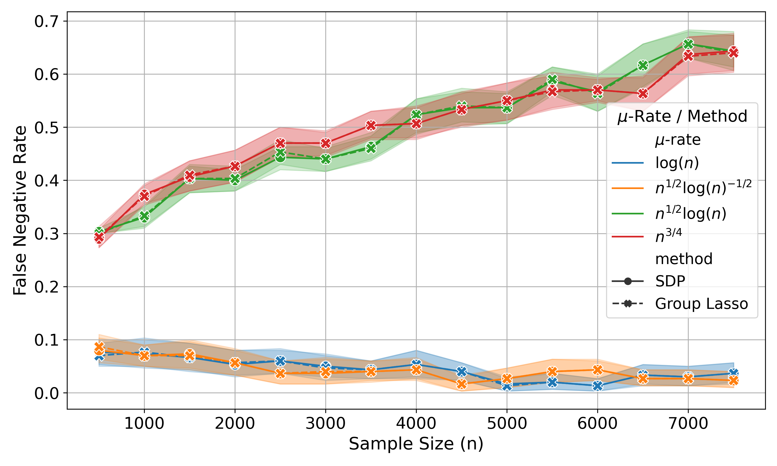
Refer to caption
Figure 1: False negative rate of I⋆{I_{\star}} without Step 4 in Algorithm 1, across different coherence levels μ\mu. Each curve corresponds to a different rate of the incoherence parameter μ\mu, with solid lines for SDP and dashed lines for group Lasso.

6.1.2 Identifying the Recovery Threshold

We next investigate the effect of the signal strength constant CC in the theoretical threshold σB=C​n−1/4​log1/4⁡n\sigma_{B}=Cn^{-1/4}\log^{1/4}n. We first vary C∈{0.8,1.2,1.6,2.0,2.4}C\in\{0.8,1.2,1.6,2.0,2.4\} and generate 𝑩⋆{\boldsymbol{B}}^{\star} using Algorithm 3. To assess recovery under heteroscedastic noise, we sample Wi​j∼𝒩​(0,σi​j2)W_{ij}\sim\mathcal{N}(0,\sigma_{ij}^{2}) with σi​j\sigma_{ij} uniformly drawn from [σmin,σmax][\sigma_{\min},\sigma_{\max}]. The node support size is set to m=10m=10.

Figure 2 shows the results of this experiment. We observe a phase transition at C≈1.6C\approx 1.6:

  1. 1.

    When C≤1.2C\leq 1.2, the FNR increases with nn, indicating recovery failure.

  2. 2.

    When C≥2.0C\geq 2.0, the FNR converges to zero.

  3. 3.

    At the threshold C=1.6C=1.6, the FNR stabilizes around 0.30.3.

These observations align closely with the theoretical predictions in Remark 5, which identifies the signal-to-noise ratio (SNR) threshold

SNR=Ω​(n1/4​log1/4⁡n)\operatorname{SNR}=\Omega(n^{1/4}\log^{1/4}n)

as the minimum rate required for exact recovery of the node support I⋆{I_{\star}}. Below this threshold, no estimator can succeed uniformly over the class of node-sparse signals. Our empirical findings support this characterization: when CC is too small, the effective SNR falls below the exact recovery threshold, and recovery fails. Both SDP and group Lasso perform similarly in this setting, and are robust to heteroscedasticity when Assumption 2 is satisfied.

Recall from Remark 5 that the partial recovery threshold is given by

SNR=Ω​(n1/4​log1/4⁡(nm)).\operatorname{SNR}=\Omega\left(n^{1/4}\log^{1/4}\left(\frac{n}{m}\right)\right).

When m=10m=10, this threshold has the same asymptotic form as the exact recovery threshold, differing only in the constant factor. The stablization of the FNR around 0.30.3 at C=1.6C=1.6 provides empirical support for this theoretical prediction, suggesting that C=1.6C=1.6 lies in the regime of partial recovery.

To investigate the partial recovery threshold in finer detail, we further vary the signal strength constant over a denser grid: C∈{1.3,1.4,1.5,1.6,1.7,1.8}C\in\{1.3,1.4,1.5,1.6,1.7,1.8\}. For each combination of sample size nn, signal strength CC, and method, we repeat the experiment 100100 times and compute the FNR for each trial. The results, summarized in Figure 3, show that as nn increases, the FNR converges to a stable value for each fixed CC. Notably, stronger signals yield better limiting FNRs: for example, when C=1.3C=1.3, the FNR levels off around 0.70.7, while for C=1.8C=1.8, it approaches 0.10.1. This trend aligns with the theoretical prediction based on the partial recovery threshold in Remark 5.
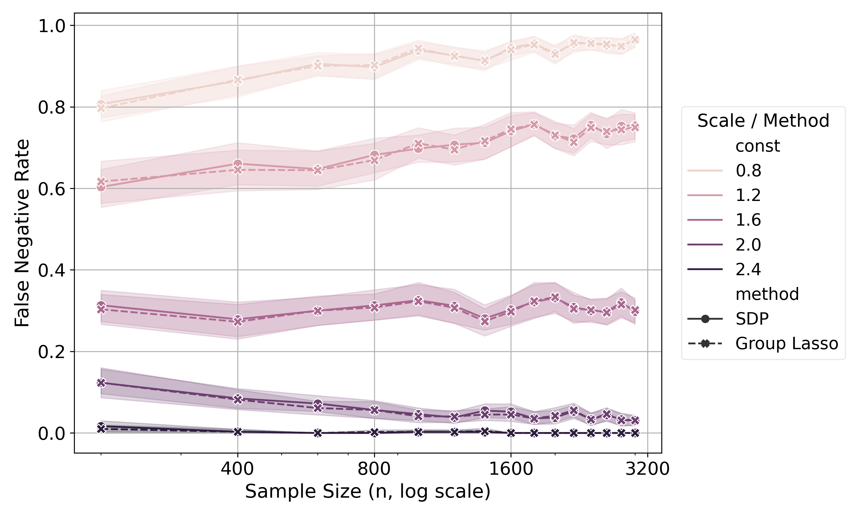
Refer to caption
Figure 2: False negative rate of I⋆{I_{\star}} for SDP and group Lasso under varying signal strength constant CC in σB=C​n−1/4​log1/4⁡n\sigma_{B}=Cn^{-1/4}\log^{1/4}n. Each color corresponds to a different value of the scale parameter C∈{0.8,1.2,1.6,2.0,2.4}C\in\{0.8,1.2,1.6,2.0,2.4\}. As CC increases, both methods transition from failure to successful recovery. A phase transition occurs near C=1.6C=1.6: when C≤1.2C\leq 1.2, the FNR remains high and increases with nn; when C≥2.0C\geq 2.0, the FNR decays toward zero. Both SDP and group Lasso perform similarly in this heteroscedastic setting.
Refer to caption
Figure 3: False negative rate of I⋆{I_{\star}} for SDP and group Lasso under varying signal strength constant CC in σB=C​n−1/4​log1/4⁡n\sigma_{B}=Cn^{-1/4}\log^{1/4}n. Each color corresponds to a different value of the scale parameter C∈{1.3,1.4,1.5,1.6,1.7,1.8}C\in\{1.3,1.4,1.5,1.6,1.7,1.8\}. As the matrix dimension nn increases, all curves eventually stablize around some constant FNRs, with larger CC leading to lower FNRs. Both SDP and group Lasso perform similarly in this heteroscedastic setting.

6.1.3 Failure Case for Group Lasso

We now demonstrate a failure mode for group Lasso by constructing a signal matrix 𝑩⋆{\boldsymbol{B}}^{\star} that satisfies the sparsity assumption but induces misleading group-level structure. Our construction is similar to Equation (41) in Theorem 14.

We set the number of signal nodes to m=⌊2​n⌋m=\lfloor 2\sqrt{n}\rfloor and define an augmented support set I⋆∪J{I_{\star}}\cup J of size m+km+k, where k=max⁡{5,⌊0.2​m⌋}k=\max\{5,\lfloor 0.2m\rfloor\}. We randomly select m+km+k nodes without replacement and let I⋆{I_{\star}} denote the first mm indices (true signal nodes) and JJ the remaining kk indices (perturbation nodes). The signal matrix 𝑩⋆{\boldsymbol{B}}^{\star} is constructed as follows:

  1. 1.

    For each (i,j)∈I⋆×J(i,j)\in{I_{\star}}\times J (and symmetrically (j,i)(j,i)), set Bi​j⋆=β1B^{\star}_{ij}=\beta_{1}, where β1=2.5​(n​log⁡n)1/4m\beta_{1}=\frac{2.5(n\log n)^{1/4}}{\sqrt{m}}.

  2. 2.

    For each i∈I⋆i\in{I_{\star}} and j∉I⋆∪Jj\notin{I_{\star}}\cup J, set Bi​j⋆=β2B^{\star}_{ij}=\beta_{2}, where β2=2​n−1/4​log1/4⁡n\beta_{2}=2n^{-1/4}\log^{1/4}n.

  3. 3.

    All other entries of 𝑩⋆{\boldsymbol{B}}^{\star} are set to zero.

This construction creates two types of signal entries in 𝑩{\boldsymbol{B}}: a few relatively large entries, corresponding to entries indexed by an element of I⋆{I_{\star}} and an element of JJ, and many weaker entries corresponding to entries indexed by an index in I⋆{I_{\star}} and the rest of the nodes. Under this setting, although nodes in I⋆{I_{\star}} have signal strength above the exact recovery threshold given in Remark 5, the group Lasso struggles to separate JJ and I⋆{I_{\star}} due to its greedy selection mechanism.

We apply both SDP and group Lasso to the observed matrix 𝒀=𝑩⋆+𝑾\boldsymbol{Y}={\boldsymbol{B}}^{\star}+\boldsymbol{W} to recover the support I⋆{I_{\star}}. As shown in Table 1, the SDP method consistently achieves exact support recovery across all sample sizes considered, since the signal in 𝑩⋆{\boldsymbol{B}}^{\star} is well above the exact recovery threshold. In contrast, group Lasso exhibits persistent recovery failure, with its false negative rate stabilizing around 0.20.2. This value aligns with the fraction k/(m+k)k/(m+k) of perturbation nodes, suggesting that group Lasso tends to select the larger-magnitude but spurious connections to JJ rather than the true support. These empirical observations corroborate the theoretical limitations of group Lasso established in Theorem 14.

Table 1: False negative rate (FNR) in recovering I⋆{I_{\star}} of SDP and group Lasso across various sample sizes. Each value is reported as the mean (standard deviation) over 5050 repeated trials.
Sample Size (nn) SDP FNR Group Lasso FNR
200 0.000 (0.000) 0.152 (0.026)
1200 0.000 (0.000) 0.168 (0.016)
2200 0.000 (0.000) 0.180 (0.012)
3200 0.000 (0.000) 0.181 (0.009)
4200 0.000 (0.000) 0.184 (0.007)
5200 0.000 (0.000) 0.184 (0.007)
6200 0.000 (0.000) 0.189 (0.006)
7200 0.000 (0.000) 0.190 (0.005)

6.1.4 Multiple Copies versus Single Copy in SDP

In Section 4.1, we established that the SDP method requires Assumption 2 to recover the node support I⋆{I_{\star}} of 𝑩⋆{\boldsymbol{B}}^{\star} when there is only one observed copy of 𝑩⋆{\boldsymbol{B}}^{\star}. We demonstrate that access to multiple copies allows us to relax Assumption 2 as shown in Theorem 11. Set the node support size m=⌈2​log⁡n⌉m=\lceil 2\log n\rceil and generate 𝒀1=𝑩⋆+𝑾1\boldsymbol{Y}_{1}={\boldsymbol{B}}^{\star}+\boldsymbol{W}_{1} and 𝒀2=𝑩⋆+𝑾2\boldsymbol{Y}_{2}={\boldsymbol{B}}^{\star}+\boldsymbol{W}_{2}, where noise is constructed as follows:

  1. 1.

    For each row ii, sample σi∼Unif⁡[σmin,σmax]\sigma_{i}\sim\operatorname{Unif}[\sigma_{\min},\sigma_{\max}], with σmin=0.8\sigma_{\min}=0.8 and σmax=1.3\sigma_{\max}=1.3.

  2. 2.

    Set the ii-th row of 𝚺0\boldsymbol{\Sigma}_{0} to σi2\sigma_{i}^{2} and define 𝚺=𝚺0+𝚺0⊤\boldsymbol{\Sigma}=\boldsymbol{\Sigma}_{0}+\boldsymbol{\Sigma}_{0}^{\top}.

  3. 3.

    Generate a symmetric matrix 𝑾0\boldsymbol{W}_{0} as before and let 𝑾=𝑾0∘𝚺\boldsymbol{W}=\boldsymbol{W}_{0}\circ\boldsymbol{\Sigma}.

This setup yields symmetric but row-heteroscedastic noise. We apply two versions of SDP, where for the multiple-copy SDP, the cost matrix is 𝒀1∘𝒀2\boldsymbol{Y}_{1}\circ\boldsymbol{Y}_{2}, and for the single-copy SDP, the cost matrix is 𝒀avg∘𝒀avg\boldsymbol{Y}_{\mathrm{avg}}\circ\boldsymbol{Y}_{\mathrm{avg}}, where 𝒀avg=(𝒀1+𝒀2)/2\boldsymbol{Y}_{\mathrm{avg}}=(\boldsymbol{Y}_{1}+\boldsymbol{Y}_{2})/2.

The results in Figure 4 demonstrate that the single-copy SDP fails under row-heteroscedastic noise, with FNR increasing as nn grows. This aligns with the discussion at the beginning of Section 4.1, confirming that support recovery is ill-posed in the presence of row-wise heteroscedasticity. By comparison, the multiple-copy SDP accurately recovers I⋆{I_{\star}} without Assumption 2, consistent with Theorem 11.
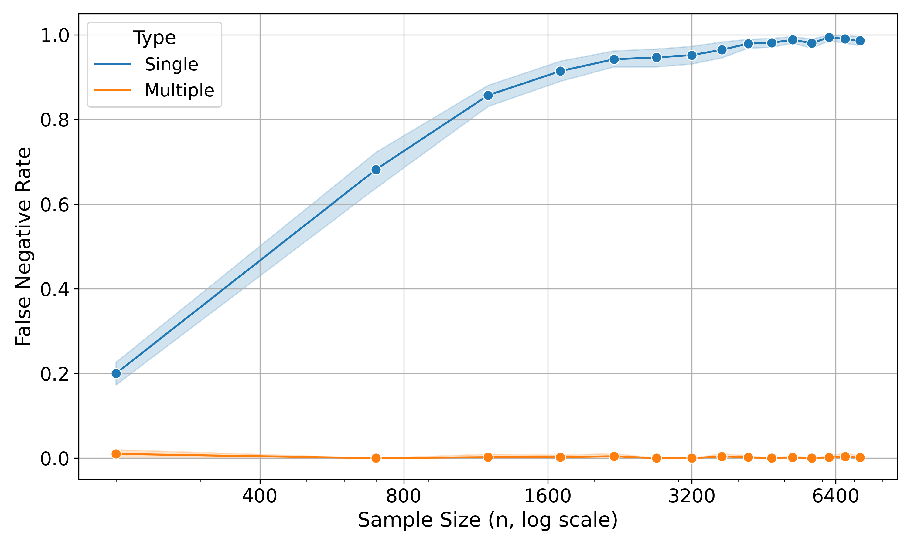
Refer to caption
Figure 4: False negative rate for recovering I⋆{I_{\star}} as a function of sample size nn (log scale), comparing two SDP-based methods: single-copy SDP (labeled “Single”) and multiple-copy SDP (labeled “Multiple”).

6.1.5 Truncated SDP for Heavy-Tailed Noise

Finally, we consider a heavy-tailed noise setting where the entries of the noise matrix are drawn i.i.d. according to a t4t_{4} distribution rescaled to have unit variance. The noise matrix 𝑾\boldsymbol{W} and signal matrix 𝑩⋆{\boldsymbol{B}}^{\star} are otherwise generated as inthe previous experiments as described in Section 6.1. We set the node support size |I⋆||{I_{\star}}| to m=⌈2​log⁡n⌉m=\lceil 2\log n\rceil and compare the performance of the vanilla SDP estimator with the truncated version that clips extreme entries, as described in Section 4.2.2. As shown in Figure 5, the truncated SDP reliably recovers I⋆{I_{\star}}, in agreement with the theoretical guarantees established in Theorem 10. Specifically, truncated SDP achieves exact support recovery under heavy-tailed noise when the signal-to-noise ratio exceeds the exact recovery threshold Θ​(n1/4​log1/4⁡n)\Theta(n^{1/4}\log^{1/4}n) defined in Remark 5. In contrast, the vanilla SDP fails under this setting, with its FNR diverging to 1 as nn increases. This behavior also aligns with Theorem 7, which indicates that when the noise magnitude LL significantly exceeds its standard deviation σ\sigma, the vanilla SDP requires a substantially higher SNR to achieve support recovery.
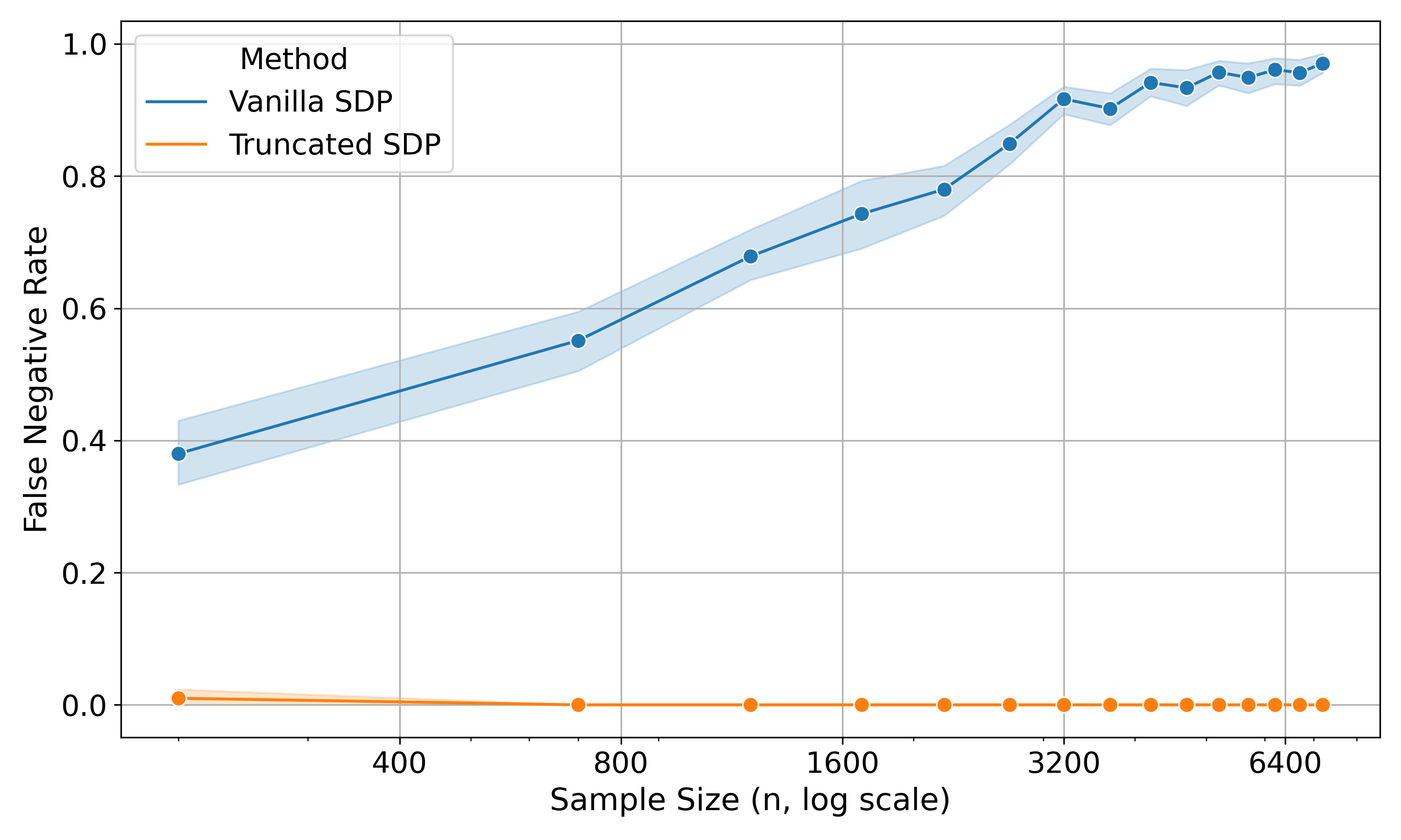
Refer to caption
Figure 5: False negative rate of recovering I⋆{I_{\star}} under scaled t4t_{4}-distributed noise as a function of sample size nn (log scale). The plot compares two methods: vanilla SDP (blue) and truncated SDP (orange).

6.2 Improved Estimation of 𝑴⋆\boldsymbol{M}^{\star}

We now empirically validate our findings from Section 5. Throughout this section, we assume access to four observations 𝒀11,𝒀12,𝒀21,𝒀22\boldsymbol{Y}_{11},\boldsymbol{Y}_{12},\boldsymbol{Y}_{21},\boldsymbol{Y}_{22} generated according to a low-rank-plus-noise model with fixed rank r=3r=3. The noise matrices are generated as described in Section 6.1. To construct the estimators, we asymmetrically arrange 𝒀i​1\boldsymbol{Y}_{i1} and 𝒀i​2\boldsymbol{Y}_{i2} to obtain 𝒀i\boldsymbol{Y}_{i} for i=1,2i=1,2.

6.2.1 Varying μ\mu and λmin⋆\lambda^{\star}_{\min}

We vary nn over a range of values from 700700 to 4000040000. The incoherence parameter μ\mu is set to either n4/5n^{4/5} or n5/6n^{5/6}, and the minimum eigenvalue of the low rank signal matrix 𝑴⋆\boldsymbol{M}^{\star} is chosen as λmin⋆∈{2.05,3}​n\lambda^{\star}_{\min}\in\{2.05,3\}\sqrt{n}. We consider three approaches to estimating 𝑼⋆{\boldsymbol{U}^{\star}} and consequently 𝑴⋆\boldsymbol{M}^{\star}:

  1. 1.

    Estimate 𝑼⋆{\boldsymbol{U}^{\star}} using the bias-corrected eigenvectors 𝑼^\widehat{\boldsymbol{U}} from Equation (63) applied to the average matrix 𝒀asym\boldsymbol{Y}_{\mathrm{asym}} of two assymetrically arranged matrices 𝒀1\boldsymbol{Y}_{1} and 𝒀2\boldsymbol{Y}_{2}. Form the estimator 𝑴^1:=𝑼^​𝚲​𝑼^⊤\widehat{\boldsymbol{M}}_{1}:=\widehat{\boldsymbol{U}}\boldsymbol{\Lambda}\widehat{\boldsymbol{U}}^{\top} as in Corollary 4, where 𝚲\boldsymbol{\Lambda} are the eigenvalues of 𝒀asym\boldsymbol{Y}_{\mathrm{asym}}.

  2. 2.

    Averaging all four matrices 𝒀i​j\boldsymbol{Y}_{ij} for i,j∈[2]i,j\in[2] and compute the top-rr eigenspace 𝑼^spec\widehat{\boldsymbol{U}}_{\mathrm{spec}} and eigenvalues 𝚲spec\boldsymbol{\Lambda}_{\mathrm{spec}} from the spectral decomposition of the average. Then form 𝑴^spec:=𝑼^spec​𝚲spec​𝑼^spec⊤\widehat{\boldsymbol{M}}_{\mathrm{spec}}:=\widehat{\boldsymbol{U}}_{\mathrm{spec}}\boldsymbol{\Lambda}_{\mathrm{spec}}\widehat{\boldsymbol{U}}_{\mathrm{spec}}^{\top} as the spectral estimator of 𝑴⋆\boldsymbol{M}^{\star}.

  3. 3.

    Use the refined eigenspace estimate 𝑼​𝚿^\boldsymbol{U}\widehat{\boldsymbol{\Psi}} from Theorem 18, and construct 𝑴^2:=𝑼​𝚿^​𝚲​𝚿^⊤​𝑼⊤\widehat{\boldsymbol{M}}_{2}:=\boldsymbol{U}\widehat{\boldsymbol{\Psi}}\boldsymbol{\Lambda}\widehat{\boldsymbol{\Psi}}^{\top}\boldsymbol{U}^{\top} as in Theorem 19, where 𝑼\boldsymbol{U} consists of the right-eigenvectors of 𝒀1\boldsymbol{Y}_{1}, and 𝚿^\widehat{\boldsymbol{\Psi}} is the bias-correction factor computed from 𝒀21\boldsymbol{Y}_{21} and 𝒀22\boldsymbol{Y}_{22} following Equations (65) to (68).

The subspace recovery and matrix entrywise recovery results are summarized in Figures 6 and 7, respectively. We highlight the following observations:

  1. 1.

    Estimation of U⋆{\boldsymbol{U}^{\star}}: The error rate of 𝑼^\widehat{\boldsymbol{U}} is the worse among all methods, since its error is dominated by the term μ/n/δmin⋆\sqrt{\mu/n}/\delta^{\star}_{\min} as given in Corollary 3, which is significantly larger compared to that of 𝑼​𝚿^\boldsymbol{U}\widehat{\boldsymbol{\Psi}} in Theorem 18 and 𝑼^spec\widehat{\boldsymbol{U}}_{\mathrm{spec}} in Theorem 21. When μ\mu is small, 𝑼^spec\widehat{\boldsymbol{U}}_{\mathrm{spec}} achieves the lowest error for smaller matrix dimension nn. As nn increases, the behavior of 𝑼^spec\widehat{\boldsymbol{U}}_{\mathrm{spec}} exhibits a clear transition: the error initially decreases with nn, then flattens, and eventually become worse than that of 𝑼​𝚿^\boldsymbol{U}\widehat{\boldsymbol{\Psi}}. This transition point depends on both μ\mu and λmin⋆\lambda^{\star}_{\min}. For instance, when μ=n4/5\mu=n^{4/5} and λmin⋆=3​n\lambda^{\star}_{\min}=3\sqrt{n}, the turning point occurs around n=8000n=8000, beyond which the error of 𝑼^spec\widehat{\boldsymbol{U}}_{\mathrm{spec}} levels off. As μ\mu increases, the transition shifts to smaller nn, while increasing λmin⋆\lambda^{\star}_{\min} delays the transition to larger nn. According to Theorem 21, this suggests that for small nn, the term σ​r​log⁡n/|λmin⋆|\sigma\sqrt{r\log n}/|\lambda^{\star}_{\min}| initially dominates the estimation error of 𝑼^spec\widehat{\boldsymbol{U}}_{\mathrm{spec}}, while the asymptotic term σ​μ​r/|λmin⋆|\sigma\sqrt{\mu r}/|\lambda^{\star}_{\min}| becomes dominant only for sufficiently large nn.

  2. 2.

    Estimation of M⋆\boldsymbol{M}^{\star}: We observe a similar trend in the estimation of 𝑴⋆\boldsymbol{M}^{\star}. The estimation error of 𝑴^1=𝑼^​𝚲​𝑼^⊤\widehat{\boldsymbol{M}}_{1}=\widehat{\boldsymbol{U}}\boldsymbol{\Lambda}\widehat{\boldsymbol{U}}^{\top} increases as λmin⋆\lambda^{\star}_{\min} increases, consistent with Corollary 4. Among all methods, the spectral estimator 𝑴^spec\widehat{\boldsymbol{M}}_{\mathrm{spec}} performs best when μ\mu is small and λmin⋆\lambda^{\star}_{\min} is large, particularly for small to moderate nn. As nn increases, the error of 𝑴^spec\widehat{\boldsymbol{M}}_{\mathrm{spec}} increases, while the error of 𝑴^2\widehat{\boldsymbol{M}}_{2} remains nearly flat or slightly decreases. Eventually, for large nn, the error of 𝑴^spec\widehat{\boldsymbol{M}}_{\mathrm{spec}} surpasses that of 𝑴^2\widehat{\boldsymbol{M}}_{2}, in line with Theorem 19, which shows that 𝑴^2\widehat{\boldsymbol{M}}_{2} achieves a better error rate than 𝑴^spec\widehat{\boldsymbol{M}}_{\mathrm{spec}} for sufficiently large nn.

Remark 14.

The estimators 𝐔​𝚿^\boldsymbol{U}\widehat{\boldsymbol{\Psi}} and 𝐌^2\widehat{\boldsymbol{M}}_{2} are likely suboptimal in terms of the leading constant in their error bounds. This inefficiency arises because they do not fully exploit the information available from all four observations: two copies are primarily used for estimation, while the remaining two are incorporated only as a correction term. It might be possible to improve the efficiency by combining the spectral estimator with 𝐔​𝚿^\boldsymbol{U}\widehat{\boldsymbol{\Psi}} and 𝐌^2\widehat{\boldsymbol{M}}_{2}, which we leave for the future work.

Refer to caption
Figure 6: Estimation error of 𝑼⋆{\boldsymbol{U}^{\star}} under the ℓ2,∞\ell_{2,\infty} norm across varying coherence μ\mu and signal strength λmin⋆\lambda^{\star}_{\min}. Each subplot corresponds to a specific pair of (μ,λmin⋆)(\mu,\lambda^{\star}_{\min}), with μ∈{n4/5,n5/6}\mu\in\{n^{4/5},n^{5/6}\} (columns, left to right) and λmin⋆∈{2.05​n,3​n}\lambda^{\star}_{\min}\in\{2.05\sqrt{n},3\sqrt{n}\} (rows, top to bottom). The estimators compared are 𝑼​𝚿^\boldsymbol{U}\widehat{\boldsymbol{\Psi}} (blue), 𝑼^\widehat{\boldsymbol{U}} (orange), and the spectral estimator 𝑼^spec\widehat{\boldsymbol{U}}_{\mathrm{spec}} (green). The yy-axis shows the ℓ2,∞\ell_{2,\infty} error on a log scale.
Refer to caption
Figure 7: Estimation error of 𝑴⋆\boldsymbol{M}^{\star} under the ℓ∞\ell_{\infty} norm across various regimes of coherence μ\mu and signal strength λmin⋆\lambda^{\star}_{\min}. Each subplot corresponds to a different combination of (μ,λmin⋆)(\mu,\lambda^{\star}_{\min}), where μ∈{n4/5,n5/6}\mu\in\{n^{4/5},n^{5/6}\} (columns, left to right) and λmin⋆∈{2.05​n,3​n}\lambda^{\star}_{\min}\in\{2.05\sqrt{n},3\sqrt{n}\} (rows, top to bottom). Three estimators are compared: 𝑼​𝚿^​𝚲​𝚿^⊤​𝑼⊤\boldsymbol{U}\widehat{\boldsymbol{\Psi}}\boldsymbol{\Lambda}\widehat{\boldsymbol{\Psi}}^{\top}\boldsymbol{U}^{\top} (blue), 𝑼^​𝚲​𝑼^⊤\widehat{\boldsymbol{U}}\boldsymbol{\Lambda}\widehat{\boldsymbol{U}}^{\top} (orange), and the spectral estimator 𝑴^spec\widehat{\boldsymbol{M}}_{\mathrm{spec}} (green).

6.2.2 Varying Eigengap Ratio

We conclude by examining the effect of the ratio ρ:=δmax⋆/δmin⋆\rho:=\delta^{\star}_{\max}/\delta^{\star}_{\min} on the estimation error rates of 𝑴⋆\boldsymbol{M}^{\star} when using the estimator 𝑴^2\widehat{\boldsymbol{M}}_{2}. We fix μ=n​log⁡n\mu=\sqrt{n}\log n and δmin⋆=log⁡n\delta^{\star}_{\min}=\log n in the experiments, and vary δmax⋆∈{log⁡n,n1/3,n1/2}\delta^{\star}_{\max}\in\{\log n,n^{1/3},n^{1/2}\}. The result is shown in Figure 8. Different values of ρ\rho yield overlapping error curves, indicating that changes in ρ\rho have negligible impact on the estimation error rates. This empirical finding suggests that the dependence on δmax⋆/δmin⋆\delta^{\star}_{\max}/\delta^{\star}_{\min} displayed by the upper bound in Theorem 19 is likely a technical artifact rather than a fundamental limitation. We leave the pursuit of this improvement to future work.

Refer to caption
Figure 8: Estimation errors of 𝑴^2:=𝑼​𝚿^​𝚲​𝚿^⊤​𝑼^⊤\widehat{\boldsymbol{M}}_{2}:=\boldsymbol{U}\widehat{\boldsymbol{\Psi}}\boldsymbol{\Lambda}\widehat{\boldsymbol{\Psi}}^{\top}\widehat{\boldsymbol{U}}^{\top} as a function of nn under the ℓ∞\ell_{\infty} norm. Each curve corresponds to a different scaling rate for the ratio ρ:=δmax⋆/δmin⋆\rho:=\delta^{\star}_{\max}/\delta^{\star}_{\min}. Each point represents the average error over 30 independent trials.

7 Discussion

In this paper, we proposed a new statistical framework for analyzing multiple weighted networks that share a low-rank structure but differ through sparse, node-specific perturbations. Our model captures a broad class of practical scenarios, extending beyond traditional multilayer network formulations that primarily address global or smooth variations across conditions.

We introduced a suite of estimation procedures that adapt to the number of observations available per group. Our approach combines spectral initialization, semidefinite programming (SDP) for support recovery, and bias-corrected refinement for improved low-rank estimation. Theoretical results establish minimax optimality under various signal and sparsity regimes, and highlight the interplay between observation multiplicity and statistical efficiency.

We further examined the limitations of commonly used alternatives such as Group Lasso, which fails under certain structured perturbation settings. In contrast, our SDP-based methods exhibit robust support recovery even under heteroscedastic and heavy-tailed noise. Comprehensive numerical experiments corroborate the theory and demonstrate key behaviors, including phase transitions, the role of coherence, and the benefits of bias-correction and multiple network observations.

Several directions for future research also emerge from our findings:

Node-sparse structure estimation.

First, a deeper understanding of the computational barriers for node-sparse recovery is needed. It remains open whether the limitations of Group Lasso observed here also apply in broader settings, such as covariance estimation. Second, while our SDP formulation is based on a least-squares loss, it is not robust to outliers. Incorporating robust loss functions (e.g., Huber or quantile-based objectives) and designing tractable algorithms under such losses would be interesting. Third, our current framework assumes continuous weights. Extending support recovery guarantees to discrete-weight networks such as binary or count-valued adjacency matrices poses both theoretical and algorithmic challenges.

Low-rank structure estimation.

The low-rank model for the control group may be oversimplified for real-world data. In many applications, the assumption of a clean low-rank plus noise decomposition may not hold. While our bias-corrected estimator achieves a near-optimal rate under the ℓ∞\ell_{\infty} norm, it only outperforms baseline methods when the matrix dimension is sufficiently large. Improving the efficiency of this estimator, especially in terms of its leading constant, would enhance its practical utility in moderate-sized problems. Moreover, the fundamental limits of low-rank matrix recovery under ℓ∞\ell_{\infty} and ℓ2,∞\ell_{2,\infty} norms with only a single observation remain unresolved. In particular, it is unclear whether a coherence-independent estimator exists for subspace recovery in this setting. Developing such an estimator, if it exists, may require substantially more sophisticated techniques.

Our results provide a foundation for future work on structure recovery in high-dimensional network models, and contribute to a broader understanding of statistical estimation under sparsity and low-rank constraints.

References

  • Agterberg and Zhang, (2024) Agterberg, J. and Zhang, A. R. (2024). Estimating higher-order mixed memberships via the ℓ2,∞\ell_{2,\infty} tensor perturbation bound. Journal of the American Statistical Association, 0(0):1–11.
  • Airoldi et al., (2008) Airoldi, E. M., Blei, D., Fienberg, S., and Xing, E. (2008). Mixed membership stochastic blockmodels. Joural of Machine Learning Research, 9:1981–2014.
  • Arroyo et al., (2021) Arroyo, J., Athreya, A., Cape, J., Chen, G., Priebe, C. E., and Vogelstein, J. T. (2021). Inference for Multiple Heterogeneous Networks with a Common Invariant Subspace. Journal of Machine Learning Research, 22(142):1–49.
  • Athreya et al., (2018) Athreya, A., Fishkind, D. E., Tang, M., Priebe, C. E., Park, Y., Vogelstein, J. T., Levin, K., Lyzinski, V., Qin, Y., and Sussman, D. L. (2018). Statistical inference on random dot product graphs: a survey. Journal of Machine Learning Research, 18(226):1–92.
  • Bakken et al., (2016) Bakken, T. E., Miller, J. A., Ding, S.-L., Sunkin, S. M., Smith, K. A., Ng, L., Szafer, A., Dalley, R. A., Royall, J. J., Lemon, T., et al. (2016). A comprehensive transcriptional map of primate brain development. Nature, 535(7612):367–375.
  • Barvinok, (1995) Barvinok, A. I. (1995). Problems of distance geometry and convex properties of quadratic maps. Discrete & Computational Geometry, 13:189–202.
  • Bassett and Sporns, (2017) Bassett, D. S. and Sporns, O. (2017). Network neuroscience. Nature Neuroscience, 20(3):353–364.
  • Benaych-Georges and Nadakuditi, (2011) Benaych-Georges, F. and Nadakuditi, R. R. (2011). The eigenvalues and eigenvectors of finite, low rank perturbations of large random matrices. Advances in Mathematics, 227(1):494–521.
  • Bhatia, (2013) Bhatia, R. (2013). Matrix Analysis, volume 169. Springer Science & Business Media.
  • Borgatti et al., (2009) Borgatti, S. P., Mehra, A., Brass, D. J., and Labianca, G. (2009). Network analysis in the social sciences. Science, 323(5916):892–895.
  • Boumal, (2023) Boumal, N. (2023). An Introduction to Optimization on Smooth Manifolds. Cambridge University Press.
  • Boumal et al., (2016) Boumal, N., Voroninski, V., and Bandeira, A. (2016). The non-convex Burer-Monteiro approach works on smooth semidefinite programs. Advances in Neural Information Processing Systems, 29.
  • Boyd et al., (2011) Boyd, S., Parikh, N., Chu, E., Peleato, B., Eckstein, J., et al. (2011). Distributed optimization and statistical learning via the alternating direction method of multipliers. Foundations and Trends in Machine Learning, 3(1):1–122.
  • Burer and Monteiro, (2003) Burer, S. and Monteiro, R. D. (2003). A nonlinear programming algorithm for solving semidefinite programs via low-rank factorization. Mathematical Programming, 95(2):329–357.
  • Butucea et al., (2018) Butucea, C., Ndaoud, M., Stepanova, N. A., and Tsybakov, A. B. (2018). Variable selection with Hamming loss. The Annals of Statistics, 46(5):1837 – 1875.
  • Cai et al., (2017) Cai, T. T., Liang, T., and Rakhlin, A. (2017). Computational and statistical boundaries for submatrix localization in a large noisy matrix. The Annals of Statistics, 45(4):1403–1430.
  • Cai and Wu, (2020) Cai, T. T. and Wu, Y. (2020). Statistical and computational limits for sparse matrix detection. The Annals of Statistics, 48(3):1593 – 1614.
  • Center for High Throughput Computing, (2006) Center for High Throughput Computing (2006). Center for high throughput computing.
  • Chen and Hero, (2017) Chen, P.-Y. and Hero, A. O. (2017). Multilayer spectral graph clustering via convex layer aggregation: theory and algorithms. IEEE Transactions on Signal and Information Processing over Networks, 3(3):553–567.
  • (20) Chen, Y., Cheng, C., and Fan, J. (2021a). Asymmetry helps: Eigenvalue and eigenvector analyses of asymmetrically perturbed low-rank matrices. The Annals of Statistics, 49(1):435.
  • (21) Chen, Y., Chi, Y., Fan, J., and Ma, C. (2021b). Spectral methods for data science: A statistical perspective. Foundations and Trends in Machine Learning, 14(5):566–806.
  • Chen and Xu, (2016) Chen, Y. and Xu, J. (2016). Statistical-computational tradeoffs in planted problems and submatrix localization with a growing number of clusters and sub-matrices. Journal of Machine Learning Research, 17(27):1–57.
  • Cheng et al., (2021) Cheng, C., Wei, Y., and Chen, Y. (2021). Tackling small eigen-gaps: Fine-grained eigenvector estimation and inference under heteroscedastic noise. IEEE Transactions on Information Theory, 67(11):7380–7419.
  • De Domenico et al., (2015) De Domenico, M., Nicosia, V., Arenas, A., and Latora, V. (2015). Structural reducibility of multilayer networks. Nature communications, 6(1):6864.
  • Diebold and Yılmaz, (2014) Diebold, F. X. and Yılmaz, K. (2014). On the network topology of variance decompositions: Measuring the connectedness of financial firms. Journal of econometrics, 182(1):119–134.
  • D’Angelo et al., (2019) D’Angelo, S., Murphy, T. B., and Alfò, M. (2019). Latent space modelling of multidimensional networks with application to the exchange of votes in Eurovision song contest. The Annals of Applied Statistics, 13(2):900–930.
  • Easley and Kleinberg, (2010) Easley, D. and Kleinberg, J. (2010). Networks, crowds, and markets: Reasoning about a highly connected world. Cambridge University Press.
  • Fan et al., (2022) Fan, J., Fan, Y., Han, X., and Lv, J. (2022). Asymptotic theory of eigenvectors for random matrices with diverging spikes. Journal of the American Statistical Association, 117(538):996–1009.
  • Fei and Chen, (2018) Fei, Y. and Chen, Y. (2018). Exponential error rates of SDP for block models: Beyond Grothendieck’s inequality. IEEE Transactions on Information Theory, 65(1):551–571.
  • Ghoshdastidar et al., (2020) Ghoshdastidar, D., Gutzeit, M., Carpentier, A., and Von Luxburg, U. (2020). Two-sample hypothesis testing for inhomogeneous random graphs. The Annals of Statistics, 48(4):2208–2229.
  • Gollini and Murphy, (2016) Gollini, I. and Murphy, T. B. (2016). Joint modeling of multiple network views. Journal of Computational and Graphical Statistics, 25(1):246–265.
  • Granovetter, (1973) Granovetter, M. S. (1973). The strength of weak ties. American Journal of Sociology, 78(6):1360–1380.
  • Guha et al., (2024) Guha, S., J. Rodriguez-Acosta, J., and Dinov, I. D. (2024). A Bayesian multiplex graph classifier of functional brain connectivity across diverse tasks of cognitive control. Neuroinformatics, 22(4):457–472.
  • Hajek et al., (2016) Hajek, B., Wu, Y., and Xu, J. (2016). Achieving exact cluster recovery threshold via semidefinite programming. IEEE Transactions on Information Theory, 62(5):2788–2797.
  • He et al., (2023) He, Y., Sun, J., Tian, Y., Ying, Z., and Feng, Y. (2023). Semiparametric modeling and analysis for longitudinal network data. arXiv preprint arXiv:2308.12227.
  • Hettmansperger and McKean, (2010) Hettmansperger, T. P. and McKean, J. W. (2010). Robust nonparametric statistical methods. CRC Press.
  • Hoff et al., (2002) Hoff, P. D., Raftery, A. E., and Handcock, M. S. (2002). Latent space approaches to social network analysis. Journal of the American Statistical Association, 97(460):1090–1098.
  • Holland et al., (1983) Holland, P. W., Laskey, K. B., and Leinhardt, S. (1983). Stochastic blockmodels: First steps. Social networks, 5(2):109–137.
  • Huber and Ronchetti, (2011) Huber, P. J. and Ronchetti, E. M. (2011). Robust Statistics. John Wiley & Sons.
  • Ingster and Suslina, (2003) Ingster, Y. and Suslina, I. A. (2003). Nonparametric goodness-of-fit testing under Gaussian models, volume 169. Springer Science & Business Media.
  • Jiang et al., (2020) Jiang, H., Kathuria, T., Lee, Y. T., Padmanabhan, S., and Song, Z. (2020). A faster interior point method for semidefinite programming. In 2020 IEEE 61st Annual Symposium on Foundations of Computer Science (FOCS), pages 910–918. IEEE.
  • Karrer and Newman, (2011) Karrer, B. and Newman, M. E. (2011). Stochastic blockmodels and community structure in networks. Physical Review E—Statistical, Nonlinear, and Soft Matter Physics, 83(1):016107.
  • Kessler et al., (2022) Kessler, D., Levin, K., and Levina, E. (2022). Prediction of network covariates using edge and node attributes. arXiv preprint arXiv:2210.17519.
  • Kivelä et al., (2014) Kivelä, M., Arenas, A., Barthelemy, M., Gleeson, J. P., Moreno, Y., and Porter, M. A. (2014). Multilayer networks. Journal of Complex Networks, 2(3):203–271.
  • Klenke, (2013) Klenke, A. (2013). Probability Theory: a comprehensive course. Springer Science & Business Media.
  • Klopp and Tsybakov, (2015) Klopp, O. and Tsybakov, A. B. (2015). Estimation of matrices with row sparsity. Problems of Information Transmission, 51(4):335–348.
  • Lei and Lin, (2023) Lei, J. and Lin, K. Z. (2023). Bias-adjusted spectral clustering in multi-layer stochastic block models. Journal of the American Statistical Association, 118(544):2433–2445.
  • Lei et al., (2024) Lei, J., Zhang, A. R., and Zhu, Z. (2024). Computational and statistical thresholds in multi-layer stochastic block models. The Annals of Statistics, 52(5):2431–2455.
  • Levin et al., (2017) Levin, K., Athreya, A., Tang, M., Lyzinski, V., and Priebe, C. E. (2017). A central limit theorem for an omnibus embedding of multiple random dot product graphs. In 2017 IEEE International Conference on Data Mining Workshops (ICDMW), pages 964–967. IEEE.
  • Levin et al., (2022) Levin, K., Lodhia, A., and Levina, E. (2022). Recovering shared structure from multiple networks with unknown edge distributions. Journal of Machine Learning Research, 23(3):1–48.
  • Li et al., (2021) Li, X., Chen, Y., and Xu, J. (2021). Convex Relaxation Methods for Community Detection. Statistical Science, 36(1):2 – 15.
  • Lovász, (2012) Lovász, L. (2012). Large Networks and Graph Limits. American Mathematical Society.
  • Ma and Wu, (2015) Ma, Z. and Wu, Y. (2015). Computational barriers in minimax submatrix detection. The Annals of Statistics, pages 1089–1116.
  • (54) MacDonald, P. W., Levina, E., and Zhu, J. (2022a). Latent process models for functional network data. arXiv preprint arXiv:2210.07491.
  • (55) MacDonald, P. W., Levina, E., and Zhu, J. (2022b). Latent space models for multiplex networks with shared structure. Biometrika, 109(3):683–706.
  • Massart, (2007) Massart, P. (2007). Concentration inequalities and model selection: Ecole d’Été de Probabilités de Saint-Flour XXXIII-2003. Springer.
  • Mohan et al., (2014) Mohan, K., London, P., Fazel, M., Witten, D., and Lee, S.-I. (2014). Node-based learning of multiple Gaussian graphical models. The Journal of Machine Learning Research, 15(1):445–488.
  • MOSEK ApS, (2025) MOSEK ApS (2025). The MOSEK Python Fusion API manual. Version 11.0.
  • Müller and Stoyan, (2002) Müller, A. and Stoyan, D. (2002). Comparison Methods for Stochastic Models and Risks. John Wiley & Sons.
  • Negahban and Wainwright, (2011) Negahban, S. and Wainwright, M. J. (2011). Estimation of (near) low-rank matrices with noise and high-dimensional scaling. The Annals of Statistics, 39(2):1069 – 1097.
  • Nielsen and Witten, (2018) Nielsen, A. M. and Witten, D. (2018). The multiple random dot product graph model. arXiv preprint arXiv:1811.12172.
  • Obozinski et al., (2011) Obozinski, G., Wainwright, M. J., and Jordan, M. I. (2011). Support union recovery in high-dimensional multivariate regression. The Annals of Statistics, 39(1):1 – 47.
  • Pataki, (1998) Pataki, G. (1998). On the rank of extreme matrices in semidefinite programs and the multiplicity of optimal eigenvalues. Mathematics of Operations Research, 23(2):339–358.
  • Paul and Chen, (2020) Paul, S. and Chen, Y. (2020). A random effects stochastic block model for joint community detection in multiple networks with applications to neuroimaging. The Annals of Applied Statistics, 14(2):993–1029.
  • Recht, (2011) Recht, B. (2011). A simpler approach to matrix completion. Journal of Machine Learning Research, 12(12).
  • Relión et al., (2019) Relión, J. D. A., Kessler, D., Levina, E., and Taylor, S. F. (2019). Network classification with applications to brain connectomics. The Annals of Applied Statistics, 13(3):1648.
  • Rubin-Delanchy et al., (2022) Rubin-Delanchy, P., Cape, J., Tang, M., and Priebe, C. E. (2022). A statistical interpretation of spectral embedding: the generalised random dot product graph. Journal of the Royal Statistical Society Series B: Statistical Methodology, 84(4):1446–1473.
  • Salter-Townshend and McCormick, (2017) Salter-Townshend, M. and McCormick, T. H. (2017). Latent space models for multiview network data. The Annals of Applied Statistics, 11(3):1217.
  • Sohn and Wein, (2025) Sohn, Y. and Wein, A. S. (2025). Sharp phase transitions in estimation with low-degree polynomials. In Proceedings of the 57th Annual ACM Symposium on Theory of Computing, STOC ’25, page 891–902, New York, NY, USA. Association for Computing Machinery.
  • Sosa and Betancourt, (2022) Sosa, J. and Betancourt, B. (2022). A latent space model for multilayer network data. Computational Statistics & Data Analysis, 169:107432.
  • Sporns, (2011) Sporns, O. (2011). The human connectome: a complex network. Annals of the New York Academy of Sciences, 1224(1):109–125.
  • Sussman et al., (2012) Sussman, D. L., Tang, M., Fishkind, D. E., and Priebe, C. E. (2012). A consistent adjacency spectral embedding for stochastic blockmodel graphs. Journal of the American Statistical Association, 107:1119–1128.
  • Tsybakov, (2008) Tsybakov, A. B. (2008). Introduction to Nonparametric Estimation. Springer.
  • Vaiana and Muldoon, (2020) Vaiana, M. and Muldoon, S. F. (2020). Multilayer brain networks. Journal of Nonlinear Science, 30(5):2147–2169.
  • Vandenberghe et al., (2005) Vandenberghe, L., Balakrishnan, V. R., Wallin, R., Hansson, A., and Roh, T. (2005). Interior-point algorithms for semidefinite programming problems derived from the kyp lemma. In Positive Polynomials in Control, pages 195–238. Springer.
  • Vandenberghe and Boyd, (1996) Vandenberghe, L. and Boyd, S. (1996). Semidefinite programming. SIAM review, 38(1):49–95.
  • Varah, (1975) Varah, J. (1975). A lower bound for the smallest singular value of a matrix. Linear Algebra and its Applications, 11(1):3–5.
  • Vershynin, (2018) Vershynin, R. (2018). High-Dimensional Probability: an Introduction with Applications in Data Science. Cambridge Series in Statistical and Probabilistic Mathematics. Cambridge University Press.
  • Wainwright, (2019) Wainwright, M. J. (2019). High-Dimensional Statistics: a Non-asymptotic Viewpoint, volume 48. Cambridge University Press.
  • Waskom, (2021) Waskom, M. L. (2021). seaborn: statistical data visualization. Journal of Open Source Software, 6(60):3021.
  • Watrigant et al., (2012) Watrigant, R., Bougeret, M., and Giroudeau, R. (2012). The k-Sparsest Subgraph Problem. Technical Report RR-12019, Université de Montpellier.
  • Xie, (2024) Xie, F. (2024). Bias-corrected joint spectral embedding for multilayer networks with invariant subspace: Entrywise eigenvector perturbation and inference. IEEE Transactions on Information Theory.
  • Yan and Levin, (2025) Yan, H. and Levin, K. (2025). Improved dependence on coherence in eigenvector and eigenvalue estimation error bounds. In Li, Y., Mandt, S., Agrawal, S., and Khan, E., editors, Proceedings of The 28th International Conference on Artificial Intelligence and Statistics, volume 258, pages 1549–1557.
  • Yang et al., (2016) Yang, D., Ma, Z., and Buja, A. (2016). Rate optimal denoising of simultaneously sparse and low rank matrices. Journal of Machine Learning Research, 17(92):1–27.
  • Young and Scheinerman, (2007) Young, S. and Scheinerman, E. (2007). Random dot product graph models for social networks. In Proceedings of the 5th International Conference on Algorithms and Models for the Web-Graph, pages 138–149.
  • Yu, (1997) Yu, B. (1997). Assouad, Fano, and Le Cam. In Festschrift for Lucien Le Cam: research papers in probability and statistics, pages 423–435. Springer.
  • Zhang et al., (2022) Zhang, A. R., Cai, T. T., and Wu, Y. (2022). Heteroskedastic PCA: Algorithm, optimality, and applications. The Annals of Statistics, 50(1):53–80.
  • Zhang et al., (2023) Zhang, J., Sun, W. W., and Li, L. (2023). Generalized connectivity matrix response regression with applications in brain connectivity studies. Journal of Computational and Graphical Statistics, 32(1):252–262.
  • Zhou and Chen, (2025) Zhou, Y. and Chen, Y. (2025). Deflated HeteroPCA: Overcoming the curse of ill-conditioning in heteroskedastic PCA. The Annals of Statistics, 53(1):91–116.

Appendix

Appendix A Proof of Theorem 4

Proof.

To analyze the LSE, the high level idea is to make use of the optimality condition of the LSE that the I^\hat{I} is a solution to the optimization problem in Equation (10). Combining with standard concentration inequalities yields the exact and partial recovery results for the LSE. Below, we first prove a few concentration inequalities.

m−km-kkkkkkk
Figure 9: The overlap pattern of II and I⋆{I_{\star}} when I⋆=[m]{I_{\star}}=[m] and |I∩I⋆|=m−k|I\cap{I_{\star}}|=m-k.

Without loss of generality, we assume that I⋆=[m]{I_{\star}}=[m]. Let I⊂[n]I\subset[n] be any set of size |I|=m|I|=m and |I∩I⋆|=m−k|I\cap{I_{\star}}|=m-k. A demonstration of the overlapping pattern of the rows and columns indexed by II and I⋆{I_{\star}} is shown in Figure 9. Let

𝒮I:={(i,j)∈[n]×[n]:i<j,i∈I}\mathcal{S}_{I}:=\left\{(i,j)\in[n]\times[n]:i<j,i\in I\right\}

and, for each k∈[m]k\in[m], define

Nk=k​(n−m)+k/2−k2/2,N_{k}=k(n-m)+k/2-k^{2}/2, (73)

which is precisely the cardinality of the set 𝒮I∖𝒮I⋆\mathcal{S}_{I}\setminus\mathcal{S}_{{I_{\star}}} when |I∩I⋆|=m−k|I\cap{I_{\star}}|=m-k. Under the assumption that n≥3​mn\geq 3m, we have that Nk=Ω​(k​n)N_{k}=\Omega(kn) for all k∈[m]k\in[m].

We first fix a k∈[m]k\in[m]. With index set II fixed, we proceed to bound the sum of squares for Wi​jW_{ij} in the purple shaded region shown in Figure 9, which has NkN_{k} entries in total. It follows from Lemma 38 that for tk>0t_{k}>0,

ℙ​[|∑(i,j)∈𝒮I−𝒮I⋆(Wi​j2−𝔼​Wi​j2)|≥tk]≤2​exp⁡(−12​min⁡{tk2Nk​L2​σ2,tkL2}).\displaystyle\mathbb{P}\left[\left|\sum_{(i,j)\in\mathcal{S}_{I}-\mathcal{S}_{{I_{\star}}}}(W_{ij}^{2}-\mathbb{E}W_{ij}^{2})\right|\geq t_{k}\right]\leq 2\exp\left(-\frac{1}{2}\min\left\{\frac{t_{k}^{2}}{N_{k}L^{2}\sigma^{2}},\frac{t_{k}}{L^{2}}\right\}\right).

Since there are (n−mk)\binom{n-m}{k} choices for I∩I⋆cI\cap{{I_{\star}}}^{c}, an application of the union bound yields

ℙ​[maxI⊂[n]I∩[m]c=k⁡|∑(i,j)∈𝒮I∖𝒮I⋆(Wi​j2−𝔼​Wi​j2)|≥tk]\displaystyle\mathbb{P}\left[\max_{\begin{subarray}{c}I\subset[n]\\ I\cap[m]^{c}=k\end{subarray}}\left|\sum_{(i,j)\in\mathcal{S}_{I}\setminus\mathcal{S}_{{I_{\star}}}}\!\!\!\!(W_{ij}^{2}-\mathbb{E}W_{ij}^{2})\right|\geq t_{k}\right] ≤2​(n−mk)​exp⁡(−12​min⁡{tk2Nk​L2​σ2,tkL2})\displaystyle\leq 2\binom{n-m}{k}\exp\!\left(-\frac{1}{2}\min\left\{\frac{t_{k}^{2}}{N_{k}L^{2}\sigma^{2}},\frac{t_{k}}{L^{2}}\right\}\right)
≤2​(e​nk)k​exp⁡(−12​min⁡{tk2Nk​L2​σ2,tkL2})\displaystyle\leq 2\left(\frac{en}{k}\right)^{k}\exp\!\left(-\frac{1}{2}\min\left\{\frac{t_{k}^{2}}{N_{k}L^{2}\sigma^{2}},\frac{t_{k}}{L^{2}}\right\}\right)
≤2​exp⁡(2​k​log⁡(nk)−12​min⁡{tk2Nk​L2​σ2,tkL2}),\displaystyle\leq 2\exp\!\left(2k\log\left(\frac{n}{k}\right)-\frac{1}{2}\min\!\left\{\frac{t_{k}^{2}}{N_{k}L^{2}\sigma^{2}},\frac{t_{k}}{L^{2}}\right\}\right),

where the last inequality holds from the fact that k≤mk\leq m and our assumption that n>3​mn>3m. Setting

tk=C​max⁡{L​σ​k​n​log⁡(nk),L2​k​log⁡(nk)},t_{k}=C\max\left\{L\sigma k\sqrt{n\log\left(\frac{n}{k}\right)},L^{2}k\log\left(\frac{n}{k}\right)\right\},

for a suitably large constant C>0C>0, it holds for for any k∈[m]k\in[m] that

maxI⊂[n]I∩[m]c=k⁡|∑(i,j)∈𝒮I−𝒮I⋆(Wi​j2−𝔼​Wi​j2)|≥C​max⁡{L​σ​k​n​log⁡(nk),L2​k​log⁡(nk)}\max_{\begin{subarray}{c}I\subset[n]\\ I\cap[m]^{c}=k\end{subarray}}\left|\sum_{(i,j)\in\mathcal{S}_{I}-\mathcal{S}_{{I_{\star}}}}(W_{ij}^{2}-\mathbb{E}W_{ij}^{2})\right|\geq C\max\left\{L\sigma k\sqrt{n\log\left(\frac{n}{k}\right)},L^{2}k\log\left(\frac{n}{k}\right)\right\} (74)

holds with probability at most O​((k/n)7​k)O(\left(k/n\right)^{7k}), where we have used Equation (73) to bound the probability that Equation (74) fails to hold.

Observing that

∑k=1m(kn)7​k=O​(n−7),\sum_{k=1}^{m}\left(\frac{k}{n}\right)^{7k}=O(n^{-7}),

a second union bound over all k∈[m]k\in[m] yields that for all suitably large nn, with probability at least 1−O​(n−7)1-O(n^{-7}), it holds for all k∈[m]k\in[m] that

maxI⊂[n],I∩[m]c=k⁡|∑(i,j)∈𝒮I−𝒮I⋆(Wi​j2−𝔼​Wi​j2)|≤C​max⁡{L​σ​k​n​log⁡(nk),L2​k​log⁡(nk)}.\displaystyle\max_{I\subset[n],I\cap[m]^{c}=k}\left|\sum_{(i,j)\in\mathcal{S}_{I}-\mathcal{S}_{{I_{\star}}}}(W_{ij}^{2}-\mathbb{E}W_{ij}^{2})\right|\leq C\max\left\{L\sigma k\sqrt{n\log\left(\frac{n}{k}\right)},L^{2}k\log\left(\frac{n}{k}\right)\right\}. (75)

By the same argument, this time applied to the sum of squares of Wi​jW_{ij} in the orange shaded region in Figure 9, it holds with probability at least 1−O​(n−7)1-O(n^{-7}) that for all k∈[m]k\in[m],

maxI⊂[n],I∩[m]c=k\displaystyle\max_{I\subset[n],I\cap[m]^{c}=k} |∑(i,j)∈𝒮I⋆−𝒮I(Wi​j2−𝔼​Wi​j2)|≤C​max⁡{L​σ​k​n​log⁡(nk),L2​k​log⁡(nk)}.\displaystyle\left|\sum_{(i,j)\in\mathcal{S}_{{I_{\star}}}-\mathcal{S}_{I}}(W_{ij}^{2}-\mathbb{E}W_{ij}^{2})\right|\leq C\max\left\{L\sigma k\sqrt{n\log\left(\frac{n}{k}\right)},L^{2}k\log\left(\frac{n}{k}\right)\right\}. (76)

We now bound the sum of Wi​j​Bi​j⋆W_{ij}B^{\star}_{ij} terms corresponding to entries in the orange shaded region shown in Figure 9. Under the condition in Equation (15), we have

maxi,j∈𝒮I⋆−𝒮I⁡|Bi​j⋆|(∑i,j∈𝒮I⋆−𝒮IBi​j⋆2)1/2=O​(k−1/2​log−1/2⁡(nk)).\frac{\max_{i,j\in\mathcal{S}_{{I_{\star}}}-\mathcal{S}_{I}}|B^{\star}_{ij}|}{\left(\sum_{i,j\in\mathcal{S}_{{I_{\star}}}-\mathcal{S}_{I}}B^{\star 2}_{ij}\right)^{1/2}}=O\left(k^{-1/2}\log^{-1/2}\left(\frac{n}{k}\right)\right). (77)

Applying standard sub-exponential tail bounds (Vershynin, 2018), it holds for any I⊂[n]I\subset[n] with |I∩I⋆|=k∈[m]|I\cap{I_{\star}}|=k\in[m] that

ℙ​(|∑(i,j)∈𝒮I⋆−𝒮IBi​j⋆​Wi​j|≥t)\displaystyle\mathbb{P}\left(\left|\sum_{(i,j)\in\mathcal{S}_{{I_{\star}}}-\mathcal{S}_{I}}\!\!B^{\star}_{ij}W_{ij}\right|\geq t\right) ≤2​exp⁡(−12​min⁡{t2σ2​∑(i,j)∈𝒮I⋆−𝒮IBi​j⋆2,tL​max(i,j)∈𝒮I⋆−𝒮I⁡|Bi​j⋆|}).\displaystyle\leq 2\exp\left(-\frac{1}{2}\min\left\{\frac{t^{2}}{\sigma^{2}\sum_{(i,j)\in\mathcal{S}_{{I_{\star}}}-\mathcal{S}_{I}}B^{\star 2}_{ij}},\frac{t}{L\max_{(i,j)\in\mathcal{S}_{{I_{\star}}}-\mathcal{S}_{I}}|B^{\star}_{ij}|}\right\}\right).

Taking

t=C​max⁡{σ​(∑(i,j)∈𝒮I⋆−𝒮IBi​j⋆2)1/2​k​log⁡(nk),L​maxi,j∈𝒮I⋆−𝒮I⁡|Bi​j⋆|⋅k​log⁡(nk)}t=C\max\left\{\sigma\left(\sum_{(i,j)\in\mathcal{S}_{{I_{\star}}}-\mathcal{S}_{I}}B^{\star 2}_{ij}\right)^{1/2}\sqrt{k\log\left(\frac{n}{k}\right)},L\max_{i,j\in\mathcal{S}_{{I_{\star}}}-\mathcal{S}_{I}}|B^{\star}_{ij}|\cdot k\log\left(\frac{n}{k}\right)\right\}

and applying a union bound over k∈[m]k\in[m] and I⊂[n]I\subset[n] such that |I∩I⋆|=k∈[m]|I\cap{I_{\star}}|=k\in[m], it holds with probability at least 1−O​(n−7)1-O(n^{-7}), for all k∈[m]k\in[m] and I⊆[n]I\subseteq[n] with |I∩I⋆|=k|I\cap{I_{\star}}|=k that,

|∑(i,j)∈𝒮I⋆−𝒮IBi​j⋆​Wi​j|\displaystyle\left|\sum_{(i,j)\in\mathcal{S}_{{I_{\star}}}-\mathcal{S}_{I}}B^{\star}_{ij}W_{ij}\right| (78)
≤C​max⁡{σ​(∑(i,j)∈𝒮I⋆−𝒮IBi​j⋆2)1/2​k​log⁡(nk),L​max(i,j)∈𝒮I⋆−𝒮I⁡|Bi​j⋆|⋅k​log⁡(nk)}\displaystyle~~\leq C\max\left\{\sigma\left(\sum_{(i,j)\in\mathcal{S}_{{I_{\star}}}-\mathcal{S}_{I}}B^{\star 2}_{ij}\right)^{1/2}\sqrt{k\log\left(\frac{n}{k}\right)},L\max_{(i,j)\in\mathcal{S}_{{I_{\star}}}-\mathcal{S}_{I}}|B^{\star}_{ij}|\cdot k\log\left(\frac{n}{k}\right)\right\}
≤C​max⁡{σ​(∑(i,j)∈𝒮I⋆−𝒮IBi​j⋆2)1/2​k​log⁡(nk),o​(L​σ​k​n​log⁡(nk))}\displaystyle~~\leq C\max\left\{\sigma\left(\sum_{(i,j)\in\mathcal{S}_{{I_{\star}}}-\mathcal{S}_{I}}B^{\star 2}_{ij}\right)^{1/2}\sqrt{k\log\left(\frac{n}{k}\right)},o\left(L\sigma k\sqrt{n\log\left(\frac{n}{k}\right)}\right)\right\}

where the last inequality follows from the condition in Equation (13).

For a matrix 𝑩{\boldsymbol{B}} and a set I⊆[n]I\subseteq[n], we define the matrix 𝑩I=(BI,i​j)1≤i,j≤n∈ℝn×n{\boldsymbol{B}}_{I}=(B_{I,ij})_{1\leq i,j\leq n}\in\mathbb{R}^{n\times n} according to

BI,i​j={Bi​j if ​(i,j)∈I×I,0 otherwise.B_{I,ij}=\begin{cases}B_{ij}&\mbox{ if }(i,j)\in I\times I,\\ 0&\mbox{ otherwise.}\end{cases} (79)

For a matrix 𝑨\boldsymbol{A}, we let ℳ​(𝑨)\mathcal{M}(\boldsymbol{A}) denote the masked matrix whose upper triangle is filled with entries of 𝑨\boldsymbol{A} and the lower triangle is all zero. To establish exact recovery for the LSE I^\hat{I}, we start with the basic inequality. By the optimality of LSE, we have

‖ℳ​(𝒀I^c)‖F2=‖ℳ​(𝑩I^c⋆+𝑾I^c)‖F2≤‖ℳ​(𝒀I⋆c)‖F2=‖ℳ​(𝑾I⋆c)‖F2.\|\mathcal{M}(\boldsymbol{Y}_{\hat{I}^{c}})\|_{\mathrm{F}}^{2}=\|\mathcal{M}({\boldsymbol{B}}^{\star}_{\hat{I}^{c}}+\boldsymbol{W}_{\hat{I}^{c}})\|_{\mathrm{F}}^{2}\leq\|\mathcal{M}(\boldsymbol{Y}_{I_{\star}^{c}})\|_{\mathrm{F}}^{2}=\|\mathcal{M}(\boldsymbol{W}_{I_{\star}^{c}})\|_{\mathrm{F}}^{2}.

Expanding the squared Frobenius norm and rearranging terms, we have

‖ℳ​(𝑩I^c⋆)‖F2+2​⟨ℳ​(𝑩I^c⋆),ℳ​(𝑾I^c)⟩≤‖ℳ​(𝑾I⋆c)‖F2−‖ℳ​(𝑾I^c)‖F2.\displaystyle\|\mathcal{M}({\boldsymbol{B}}^{\star}_{\hat{I}^{c}})\|_{\mathrm{F}}^{2}+2\langle\mathcal{M}({\boldsymbol{B}}^{\star}_{\hat{I}^{c}}),\mathcal{M}(\boldsymbol{W}_{\hat{I}^{c}})\rangle\leq\|\mathcal{M}(\boldsymbol{W}_{I_{\star}^{c}})\|_{\mathrm{F}}^{2}-\|\mathcal{M}(\boldsymbol{W}_{\hat{I}^{c}})\|_{\mathrm{F}}^{2}. (80)

We will now show that in order for Equation (80) to hold, we must have |I^∩I⋆|=m|\hat{I}\cap{I_{\star}}|=m with high probability under the condition given in Equation (14). If for some k∈[m]k\in[m], |I^∩I⋆|=m−k|\hat{I}\cap{I_{\star}}|=m-k, combining Equations (75)-(78) into Equation (80) yields that with probability at least 1−O​(n−7)1-O(n^{-7}), we have

‖ℳ​(𝑩I^c⋆)‖F2\displaystyle\|\mathcal{M}({\boldsymbol{B}}^{\star}_{\hat{I}^{c}})\|_{\mathrm{F}}^{2} ≤C​σ​‖ℳ​(𝑩I^c⋆)‖F​k​log⁡(nk)+C​L​σ​k​n​log⁡(nk)\displaystyle\leq C\sigma\|\mathcal{M}({\boldsymbol{B}}^{\star}_{\hat{I}^{c}})\|_{\mathrm{F}}\sqrt{k\log\left(\frac{n}{k}\right)}+CL\sigma k\sqrt{n\log\left(\frac{n}{k}\right)}

where the second inequality follows from Equation (73). Taking square roots, it follows that

‖ℳ​(𝑩I^c⋆)‖F\displaystyle\|\mathcal{M}({\boldsymbol{B}}^{\star}_{\hat{I}^{c}})\|_{F} ≤C​(L​σ​k)1/2​n1/4​log1/4⁡(nk).\displaystyle\leq C(L\sigma k)^{1/2}n^{1/4}\log^{1/4}\left(\frac{n}{k}\right).

Noting that by the condition in Equation (14), we have

‖ℳ​(𝑩I^c⋆)‖F≥k​b\|\mathcal{M}({\boldsymbol{B}}^{\star}_{\hat{I}^{c}})\|_{\mathrm{F}}\geq\sqrt{k}b

where bb is defined in Equation (12), we have

b\displaystyle b ≤C​(L​σ)1/2​n1/4​log1/4⁡(nk)\displaystyle\leq C(L\sigma)^{1/2}n^{1/4}\log^{1/4}\left(\frac{n}{k}\right)

Hence, if for some k0>0k_{0}>0 and a sufficiently large constant c0>0c_{0}>0,

b≥c0​(L​σ)1/2​n1/4​log1/4⁡(nk0)b\geq c_{0}(L\sigma)^{1/2}n^{1/4}\log^{1/4}\left(\frac{n}{k_{0}}\right)

the inequality in Equation (80) cannot hold for any k≥k0k\geq k_{0} with probability at least 1−O​(n−7)1-O(n^{-7}) and therefore, we must have |I^∩I⋆|≥m−k0|\hat{I}\cap{I_{\star}}|\geq m-k_{0}. Taking k0=1k_{0}=1 yields exact recovery.

∎

Appendix B Proof of Minimax Results for Support Recovery

In this section, we provide a proof of Theorem 5, along with the proof of Corollaries 1 and 6. Several supporting technical lemmas are deferred to Section B.4.

B.1 Proof of Theorem 5

Proof.

We start with an overview of the proof strategy. Since the minimax risk is lower-bounded by the Bayes risk under any proper prior over 𝑩∈ℬS​(b,n,m){\boldsymbol{B}}\in\mathcal{B}_{S}(b,n,m) defined in Equation (17), it suffices to construct a prior for which the lower bound in Equation (18) holds. For details on minimax hypothesis testing, we refer the reader to Ingster and Suslina, (2003). Our argument proceeds in four steps:

  • •

    Step 1. We construct a hierarchical prior over the parameter set ℬS​(b,n,m)\mathcal{B}_{S}(b,n,m), and then replace it with a more tractable product prior. The Bayes risk under this product prior serves as a lower bound of the minimax risk, and is easier to analyze.

  • •

    Step 2. We reduce the Bayes risk to sum of expected errors in a sequence of nn binary hypothesis testing problems, one for each node, allowing a tractable lower bound on the Bayes risk.

  • •

    Step 3. We derive lower bound on the expected testing risk for each hypothesis by analyzing a Gaussian mixture testing problem, where the risk is defined as a weighted combination of the Type I and Type II errors.

  • •

    Step 4. Finally, we aggregate the binary hypothesis testing risks to obtain the desired lower bound on the overall Bayes risk.

Step 1: Constructing a prior.

To define a probability measure over ℬS​(b,n,m)\mathcal{B}_{S}(b,n,m), we proceed in two steps. First, we sample the binary support indicator vector 𝜼∈{0,1}n\boldsymbol{\eta}\in\{0,1\}^{n} from a prior πΘ\pi_{\Theta}, defined in Lemma 4, with parameter m′∈(0,m]m^{\prime}\in(0,m]. Conditioned on 𝜼\boldsymbol{\eta}, for each i∈[n]i\in[n]:

  • •

    If with ηi=1\eta_{i}=1, we sample the vector of entries {Bi​i}∪{Bi​j|j:ηj=0}\{B_{ii}\}\cup\{B_{ij}|j:\eta_{j}=0\} uniformly from the sphere b​𝕊n−∑j=1nηjb\mathbb{S}^{n-\sum_{j=1}^{n}\eta_{j}}. For Bi​jB_{ij} where i≠ji\neq j and ηi=ηj=1\eta_{i}=\eta_{j}=1, we set Bi​jB_{ij} to be a small fixed nonzero value, for example, Bi​j=σ/nB_{ij}=\sigma/n.

  • •

    If ηi=0\eta_{i}=0, for j∈[n]j\in[n] and ηj=0\eta_{j}=0, we set Bi​j=0B_{ij}=0.

By definition of ℬS​(b,n,m)\mathcal{B}_{S}(b,n,m), the prior must exclude the set

ℰ:={𝑩∈Sym(n),|I𝑩|≤m:∥𝑩i,⋅∥0≤m for all i∈I𝑩},\mathcal{E}:=\left\{{\boldsymbol{B}}\in\operatorname{Sym}(n),|I_{\boldsymbol{B}}|\leq m:\|{\boldsymbol{B}}_{i,\cdot}\|_{0}\leq m\text{ for all }i\in I_{\boldsymbol{B}}\right\},

which includes matrices that violate Assumption 3, thereby making the node support I𝑩I_{{\boldsymbol{B}}} potentially non-identifiable. However, since the event ℰc\mathcal{E}^{c} occurs almost surely under our construction (since ‖𝑩i,⋅‖0>m\|{\boldsymbol{B}}_{i,\cdot}\|_{0}>m occurs almost surely), including it does not affect the resulting Bayes risk. Thus, for notational and technical simplicity, we proceed with the sampling distribution defined above. Under ℬS​(b,n,m)∖ℰ\mathcal{B}_{S}(b,n,m)\setminus\mathcal{E}, the support I𝑩I_{{\boldsymbol{B}}} corresponds to the indices ii such that ηi=1\eta_{i}=1.

Although the prior πΘ\pi_{\Theta} defines a valid probability distribution over ℬS​(b,n,m)\mathcal{B}_{S}(b,n,m), computing the Bayes risk under this prior is challenging. Fortunately, we can construct a simpler distribution that yields a lower bound on the Bayes risk under πΘ\pi_{\Theta} that is easier to analyze. Let π\pi denote the product measure of nn independent Bernoulli distributions with shared parameter m′/nm^{\prime}/n. By Equation (92) in Lemma 4, we have

inf𝜼^𝔼πΘ​𝔼𝜼​‖𝜼−𝜼^‖H≥inf𝜼^∈[0,1]n𝔼π​𝔼𝜼​‖𝜼^−𝜼‖H−4​m′​exp⁡(−(m−m′)22​m),\inf_{\widehat{\boldsymbol{\eta}}}\mathbb{E}_{\pi_{\Theta}}\mathbb{E}_{\boldsymbol{\eta}}\|\boldsymbol{\eta}-\widehat{\boldsymbol{\eta}}\|_{\mathrm{H}}\geq\inf_{\widehat{\boldsymbol{\eta}}\in[0,1]^{n}}\mathbb{E}_{\pi}\mathbb{E}_{\boldsymbol{\eta}}\|\widehat{\boldsymbol{\eta}}-\boldsymbol{\eta}\|_{\mathrm{H}}-4m^{\prime}\exp\left(-\frac{\left(m-m^{\prime}\right)^{2}}{2m}\right), (81)

which implies that it suffices to analyze the Bayes risk under the simpler product prior π\pi.

Accordingly, we revise our sampling procedure as follows. First, sample 𝜼\boldsymbol{\eta} from π\pi. Then, conditioned on 𝜼\boldsymbol{\eta}, draw {Bi​i}∪{Bi​j|j:ηj=0}\{B_{ii}\}\cup\{B_{ij}|j:\eta_{j}=0\} from the uniform distribution over b​𝕊n−∑j=1nηjb\mathbb{S}^{n-\sum_{j=1}^{n}\eta_{j}}. For i,j∈[n]i,j\in[n] distinct such that ηi=ηj=1\eta_{i}=\eta_{j}=1, set Bi​jB_{ij} to be a small fixed nonzero value such as σ/n\sigma/n. In this way, we are guaranteed that I𝑩I_{{\boldsymbol{B}}} as well as 𝜼\boldsymbol{\eta} are almost surely identifiable.

Step 2: Bayes risk reduces to testing nn hypotheses.

To analyze the information available for estimating ηi\eta_{i}, define the following subsets of observed entries:

𝒀~∼i={Y~j​k:j≠i,k≠i}∪{Y~i​k:ηk=1,k≠i},and𝒚~i={Y~i​k:ηk=0}∪{Y~i​i}.\widetilde{\boldsymbol{Y}}_{\sim i}=\{\widetilde{Y}_{jk}:j\neq i,k\neq i\}\cup\{\widetilde{Y}_{ik}:\eta_{k}=1,k\neq i\},\quad\text{and}\quad\widetilde{\boldsymbol{y}}_{i}=\{\widetilde{Y}_{ik}:\eta_{k}=0\}\cup\{\widetilde{Y}_{ii}\}.

Denote

g​(𝜼,𝒀~∼i):=𝔼​[|η^i​(𝒀~)−ηi||𝜼,𝒀~∼i].g(\boldsymbol{\eta},\widetilde{\boldsymbol{Y}}_{\sim i}):=\mathbb{E}\left[\left.\left|\hat{\eta}_{i}(\widetilde{\boldsymbol{Y}})-\eta_{i}\right|\right|\boldsymbol{\eta},\widetilde{\boldsymbol{Y}}_{\sim i}\right]. (82)

By definition of the Hamming distance, we have

inf𝜼^∈[0,1]n𝔼π​𝔼𝜼​‖𝜼^−𝜼‖H\displaystyle\inf_{\widehat{\boldsymbol{\eta}}\in[0,1]^{n}}\mathbb{E}_{\pi}\mathbb{E}_{\boldsymbol{\eta}}\|\widehat{\boldsymbol{\eta}}-\boldsymbol{\eta}\|_{\mathrm{H}} ≥∑i=1ninfη^i∈[0,1]𝔼π​𝔼𝜼​|η^i​(𝒀~)−ηi|\displaystyle\geq\sum_{i=1}^{n}\inf_{\hat{\eta}_{i}\in[0,1]}\mathbb{E}_{\pi}\mathbb{E}_{\boldsymbol{\eta}}\left|\hat{\eta}_{i}(\widetilde{\boldsymbol{Y}})-\eta_{i}\right| (83)
=∑i=1ninfη^i∈[0,1]𝔼π​𝔼​[𝔼​[|η^i​(𝒀~)−ηi||𝜼,𝒀~∼i]|𝜼]\displaystyle=\sum_{i=1}^{n}\inf_{\hat{\eta}_{i}\in[0,1]}\mathbb{E}_{\pi}\mathbb{E}\left[\mathbb{E}\left.\left[\left.\left|\hat{\eta}_{i}(\widetilde{\boldsymbol{Y}})-\eta_{i}\right|\right|\boldsymbol{\eta},\widetilde{\boldsymbol{Y}}_{\sim i}\right]\right|\boldsymbol{\eta}\right]
=∑i=1ninfη^i∈[0,1]𝔼π​𝔼​[g​(𝜼,𝒀~∼i)|𝜼].\displaystyle=\sum_{i=1}^{n}\inf_{\hat{\eta}_{i}\in[0,1]}\mathbb{E}_{\pi}\mathbb{E}\left[\left.g(\boldsymbol{\eta},\widetilde{\boldsymbol{Y}}_{\sim i})\right|\boldsymbol{\eta}\right].

Recall that under the product measure π\pi, the indicator ηi\eta_{i} is independent of 𝒀~∼i\widetilde{\boldsymbol{Y}}_{\sim i} and 𝜼∼i\boldsymbol{\eta}_{\sim i}, and follows a Bernoulli distribution with parameter m′/nm^{\prime}/n, denoted π0\pi_{0}. We can rewrite Equation (83) as

inf𝜼^∈[0,1]n𝔼π​𝔼𝜼​‖𝜼^−𝜼‖H\displaystyle\inf_{\widehat{\boldsymbol{\eta}}\in[0,1]^{n}}\mathbb{E}_{\pi}\mathbb{E}_{\boldsymbol{\eta}}\|\widehat{\boldsymbol{\eta}}-\boldsymbol{\eta}\|_{\mathrm{H}} ≥∑i=1ninfη^i∈[0,1]𝔼π0n−1​𝔼π0​[𝔼​[g​(𝜼,𝒀~∼i)|𝜼]​𝜼∼i]\displaystyle\geq\sum_{i=1}^{n}\inf_{\hat{\eta}_{i}\in[0,1]}\mathbb{E}_{\pi_{0}^{n-1}}\mathbb{E}_{\pi_{0}}\left[\mathbb{E}\left[\left.g(\boldsymbol{\eta},\widetilde{\boldsymbol{Y}}_{\sim i})\right|\boldsymbol{\eta}\right]\boldsymbol{\eta}_{\sim i}\right]
=∑i=1ninfη^i∈[0,1]𝔼π0n−1​𝔼​[𝔼π0​[g​(𝜼,𝒀~∼i)|𝜼∼i,𝒀~∼i]|𝜼∼i].\displaystyle=\sum_{i=1}^{n}\inf_{\hat{\eta}_{i}\in[0,1]}\mathbb{E}_{\pi_{0}^{n-1}}\mathbb{E}\left[\left.\mathbb{E}_{\pi_{0}}\left[\left.g(\boldsymbol{\eta},\widetilde{\boldsymbol{Y}}_{\sim i})\right|\boldsymbol{\eta}_{\sim i},\widetilde{\boldsymbol{Y}}_{\sim i}\right]\right|\boldsymbol{\eta}_{\sim i}\right].

Interchanging the order of infimum and 𝔼π0n−1​𝔼\mathbb{E}_{\pi_{0}^{n-1}}\mathbb{E} in the above display and using the definition of gg in Equation (82) yields that

inf𝜼^∈[0,1]n𝔼π​𝔼𝜼​‖𝜼^−𝜼‖H\displaystyle\inf_{\widehat{\boldsymbol{\eta}}\in[0,1]^{n}}\mathbb{E}_{\pi}\mathbb{E}_{\boldsymbol{\eta}}\|\widehat{\boldsymbol{\eta}}-\boldsymbol{\eta}\|_{\mathrm{H}} (84)
≥∑i=1n𝔼π0n−1​𝔼​[infη^i∈[0,1]𝔼π0​{𝔼​[|η^i​(𝒀~)−ηi||𝜼,𝒀~∼i]|𝜼∼i,𝒀~∼i}|𝜼∼i].\displaystyle~~\geq\sum_{i=1}^{n}\mathbb{E}_{\pi_{0}^{n-1}}\mathbb{E}\left[\left.\inf_{\hat{\eta}_{i}\in[0,1]}\mathbb{E}_{\pi_{0}}\left\{\mathbb{E}\left[\left.\left|\hat{\eta}_{i}(\widetilde{\boldsymbol{Y}})-\eta_{i}\right||\boldsymbol{\eta},\widetilde{\boldsymbol{Y}}_{\sim i}\right]\right|\boldsymbol{\eta}_{\sim i},\widetilde{\boldsymbol{Y}}_{\sim i}\right\}\right|\boldsymbol{\eta}_{\sim i}\right].

Now, since ηi\eta_{i} is independent of 𝜼∼i\boldsymbol{\eta}_{\sim i} and 𝒀~∼i\widetilde{\boldsymbol{Y}}_{\sim i}, and since the only part of 𝒀~\widetilde{\boldsymbol{Y}} that depends on ηi\eta_{i} is 𝒚~i\widetilde{\boldsymbol{y}}_{i}, the inner expectation of Equation (84) reduces to

infη^i∈[0,1]𝔼π0​[𝔼​[|η^i​(𝒚~i,𝒀~∼i)−ηi||𝜼,𝒀~∼i]|𝜼∼i,𝒀~∼i]=\displaystyle\inf_{\hat{\eta}_{i}\in[0,1]}\mathbb{E}_{\pi_{0}}\left[\left.\mathbb{E}\left[\left|\hat{\eta}_{i}(\widetilde{\boldsymbol{y}}_{i},\widetilde{\boldsymbol{Y}}_{\sim i})-\eta_{i}\right||\boldsymbol{\eta},\widetilde{\boldsymbol{Y}}_{\sim i}\right]\right|\boldsymbol{\eta}_{\sim i},\widetilde{\boldsymbol{Y}}_{\sim i}\right]= infTi​(𝒚~i)∈[0,1]𝔼π0​[𝔼​[|Ti​(𝒚~i)−ηi||𝜼]|𝜼∼i],\displaystyle\inf_{T_{i}(\widetilde{\boldsymbol{y}}_{i})\in[0,1]}\mathbb{E}_{\pi_{0}}\left[\mathbb{E}\left[\left|T_{i}(\widetilde{\boldsymbol{y}}_{i})-\eta_{i}\right||\boldsymbol{\eta}\right]|\boldsymbol{\eta}_{\sim i}\right], (85)

where the infimum on the right hand side is taken over all test functions Ti​(𝒚~i)∈[0,1]T_{i}(\widetilde{\boldsymbol{y}}_{i})\in[0,1] that is a measurable function of 𝒚~i\widetilde{\boldsymbol{y}}_{i}. Taking Equation (85) into Equation (84), we have

inf𝜼^∈[0,1]n𝔼π​𝔼𝜼​‖𝜼^−𝜼‖H≥∑i=1n𝔼π0n−1​[infTi​(𝒚~i)∈[0,1]𝔼π0​[𝔼​[|Ti​(𝒚~i)−ηi||𝜼]|𝜼∼i]].\displaystyle\inf_{\widehat{\boldsymbol{\eta}}\in[0,1]^{n}}\mathbb{E}_{\pi}\mathbb{E}_{\boldsymbol{\eta}}\|\widehat{\boldsymbol{\eta}}-\boldsymbol{\eta}\|_{\mathrm{H}}\geq\sum_{i=1}^{n}\mathbb{E}_{\pi_{0}^{n-1}}\left[\inf_{T_{i}(\widetilde{\boldsymbol{y}}_{i})\in[0,1]}\mathbb{E}_{\pi_{0}}\left[\mathbb{E}\left[\left|T_{i}(\widetilde{\boldsymbol{y}}_{i})-\eta_{i}\right||\boldsymbol{\eta}\right]|\boldsymbol{\eta}_{\sim i}\right]\right]. (86)
Step 3: Lower bound the expected test errors.

Recall the sampling scheme for 𝜼\boldsymbol{\eta} and 𝑩{\boldsymbol{B}} described in Step 1. For a given 𝜼∼i\boldsymbol{\eta}_{\sim i}, the right hand side of Equation (85) corresponds to a hypothesis testing problem under a Gaussian mixture model. Let

k=n−∑j≠iηj.k=n-\sum_{j\neq i}\eta_{j}. (87)

We consider a binary random variable η∈{0,1}\eta\in\{0,1\} drawn from the prior distribution π0\pi_{0}, and define a random vector 𝒚∈ℝk\boldsymbol{y}\in\mathbb{R}^{k} according to the following mixture model:

𝒚=d{𝒘 if ​η=0,𝜽+𝒘 if ​η=1,\boldsymbol{y}\stackrel{{\scriptstyle d}}{{=}}\begin{cases}\boldsymbol{w}&\mbox{ if }\eta=0,\\ \boldsymbol{\theta}+\boldsymbol{w}&\mbox{ if }\eta=1,\end{cases}

where 𝜽∼Unif⁡(b​𝕊k−1)\boldsymbol{\theta}\sim\operatorname{Unif}(b\mathbb{S}^{k-1}) and 𝒘∼𝒩​(0,σ2​𝑰k)\boldsymbol{w}\sim\mathcal{N}(0,\sigma^{2}\boldsymbol{I}_{k}) are independent. By construction, 𝒚~i\widetilde{\boldsymbol{y}}_{i} has the same distribution as 𝒚\boldsymbol{y} and we have

infTi​(𝒚~i)∈[0,1]𝔼π0​[𝔼​[|Ti​(𝒚~i)−ηi|​𝜼]|𝜼∼i]=infT​(𝒚)∈[0,1]𝔼π0​𝔼η​[|T​(𝒚)−η|],\inf_{T_{i}(\widetilde{\boldsymbol{y}}_{i})\in[0,1]}\mathbb{E}_{\pi_{0}}[\mathbb{E}\left[\left|T_{i}(\widetilde{\boldsymbol{y}}_{i})-\eta_{i}\right|\boldsymbol{\eta}\right]|\boldsymbol{\eta}_{\sim i}]=\inf_{T(\boldsymbol{y})\in[0,1]}\mathbb{E}_{\pi_{0}}\mathbb{E}_{\eta}\left[\left|T(\boldsymbol{y})-\eta\right|\right],

where the infimum on the right hand side is taken over all test functions T​(𝒚)∈[0,1]T(\boldsymbol{y})\in[0,1] that is a measurable function of 𝒚\boldsymbol{y}. We also use the fact that η\eta is independent of 𝜼∼i\boldsymbol{\eta}_{\sim i} under the product measure π\pi to obtain the above equality.

Combining the above display with Lemma 7, when we choose a sufficiently small bb, it follows that

infTi​(𝒚~i)∈[0,1]𝔼π0​[𝔼​[|Ti​(𝒚~i)−ηi|​𝜼]|𝜼∼i]\displaystyle\inf_{T_{i}(\widetilde{\boldsymbol{y}}_{i})\in[0,1]}\mathbb{E}_{\pi_{0}}[\mathbb{E}\left[\left|T_{i}(\widetilde{\boldsymbol{y}}_{i})-\eta_{i}\right|\boldsymbol{\eta}\right]|\boldsymbol{\eta}_{\sim i}] =infT​(𝒚)∈[0,1]𝔼π0​𝔼η​[|T​(𝒚)−η|]\displaystyle=\inf_{T(\boldsymbol{y})\in[0,1]}\mathbb{E}_{\pi_{0}}\mathbb{E}_{\eta}\left[\left|T(\boldsymbol{y})-\eta\right|\right] (88)
≥m′n−m′⁣24​n2​exp⁡(b4​Ck​σ4)−3​m′⁣24​n2,\displaystyle\geq\frac{m^{\prime}}{n}-\frac{m^{\prime 2}}{4n^{2}}\exp\left(\frac{b^{4}C}{k\sigma^{4}}\right)-\frac{3m^{\prime 2}}{4n^{2}},

where C>0C>0 is a universal constant. As a reminder, kk in Equation (88) is a random quantity defined in Equation (87).

Step 4: Combining the results.

Combining Equations (86) and (88),

inf𝜼^∈[0,1]n𝔼π​𝔼𝜼​‖𝜼^−𝜼‖H≥maxm′∈(0,m]⁡[m′−3​m′⁣24​n−m′⁣24​n​𝔼​[exp⁡(b4​Ck​σ4)]].\inf_{\widehat{\boldsymbol{\eta}}\in[0,1]^{n}}\mathbb{E}_{\pi}\mathbb{E}_{\boldsymbol{\eta}}\|\widehat{\boldsymbol{\eta}}-\boldsymbol{\eta}\|_{\mathrm{H}}\geq\max_{m^{\prime}\in(0,m]}\left[m^{\prime}-\frac{3m^{\prime 2}}{4n}-\frac{m^{\prime 2}}{4n}\mathbb{E}\left[\exp\left(\frac{b^{4}C}{k\sigma^{4}}\right)\right]\right].

Defining a=C​b4/σ4a=Cb^{4}/\sigma^{4} and applying Lemma 9, we have for sufficiently large nn and 3​m<n3m<n,

inf𝜼^∈[0,1]n\displaystyle\inf_{\widehat{\boldsymbol{\eta}}\in[0,1]^{n}} 𝔼π​𝔼𝜼​‖𝜼^−𝜼‖H\displaystyle\mathbb{E}_{\pi}\mathbb{E}_{\boldsymbol{\eta}}\|\widehat{\boldsymbol{\eta}}-\boldsymbol{\eta}\|_{\mathrm{H}}
≥maxm′∈(0,m]⁡m′4​[3−m′n​(exp⁡{a−C​n​log⁡n3​m′}+exp⁡{alog⁡n−C​n}+eC​an)].\displaystyle\geq\max_{m^{\prime}\in(0,m]}\frac{m^{\prime}}{4}\left[3-\frac{m^{\prime}}{n}\left(\exp\left\{a-Cn\log\frac{n}{3m^{\prime}}\right\}+\exp\left\{\frac{a}{\log n}-Cn\right\}+e^{\frac{Ca}{n}}\right)\right].

Recalling the definition of fn​(a,m′)f_{n}(a,m^{\prime}) from the statement of Theorem 5, it follows that

inf𝜼^∈[0,1]n𝔼π​𝔼𝜼​‖𝜼^−𝜼‖H≥maxm′∈(0,m]⁡(m′4​fn​(a,m′)).\inf_{\widehat{\boldsymbol{\eta}}\in[0,1]^{n}}\mathbb{E}_{\pi}\mathbb{E}_{\boldsymbol{\eta}}\|\widehat{\boldsymbol{\eta}}-\boldsymbol{\eta}\|_{\mathrm{H}}\geq\max_{m^{\prime}\in(0,m]}\left(\frac{m^{\prime}}{4}f_{n}(a,m^{\prime})\right). (89)

Thus, combining Equations (81)-(89), we have

inf𝜼^𝔼πΘ​𝔼𝜼​‖𝜼^−𝜼‖H\displaystyle\inf_{\widehat{\boldsymbol{\eta}}}\mathbb{E}_{\pi_{\Theta}}\mathbb{E}_{\boldsymbol{\eta}}\|\widehat{\boldsymbol{\eta}}-\boldsymbol{\eta}\|_{\mathrm{H}} ≥infT∈[0,1]inf𝜼^∈[0,1]n𝔼π​𝔼𝜼​‖𝜼^−𝜼‖H−4​m′​exp⁡{−(m−m′)22​m}\displaystyle\geq\inf_{T\in[0,1]}\inf_{\widehat{\boldsymbol{\eta}}\in[0,1]^{n}}\mathbb{E}_{\pi}\mathbb{E}_{\boldsymbol{\eta}}\|\widehat{\boldsymbol{\eta}}-\boldsymbol{\eta}\|_{\mathrm{H}}-4m^{\prime}\exp\left\{-\frac{\left(m-m^{\prime}\right)^{2}}{2m}\right\}
≥maxm′∈(0,m]⁡[m′4​fn​(a,m′)−4​m′​exp⁡{−(m−m′)22​m}]\displaystyle\geq\max_{m^{\prime}\in(0,m]}\left[\frac{m^{\prime}}{4}f_{n}(a,m^{\prime})-4m^{\prime}\exp\left\{-\frac{\left(m-m^{\prime}\right)^{2}}{2m}\right\}\right]

which completes the proof. ∎

B.2 Proof of Corollary 1

Proof.

To show that exact recovery of 𝜼\boldsymbol{\eta} is infeasible, it suffices to provide a nontrivial lower bound of the Hamming risk

inf𝜼^∈[0,1]n𝔼π​𝔼𝜼​‖𝜼^−𝜼‖H.\inf_{\widehat{\boldsymbol{\eta}}\in[0,1]^{n}}\mathbb{E}_{\pi}\mathbb{E}_{\boldsymbol{\eta}}\|\widehat{\boldsymbol{\eta}}-\boldsymbol{\eta}\|_{\mathrm{H}}.

Let a=C​b4/σ4a=Cb^{4}/\sigma^{4}. For any m′∈[1,m]m^{\prime}\in[1,m], when

a<C​n​log⁡(n3​m′),a<Cn\log\left(\frac{n}{3m^{\prime}}\right),

we have

max⁡{a−C​n​log⁡(n3​m′),alog⁡n−C​n,C​an}<log⁡(n3​m′).\max\left\{a-Cn\log\left(\frac{n}{3m^{\prime}}\right),~\frac{a}{\log n}-Cn,~\frac{Ca}{n}\right\}<\log\left(\frac{n}{3m^{\prime}}\right).

Taking exponentials on both sides and applying Theorem 5, the following inequality holds:

3−m′n​(exp⁡{a−C​n​log⁡n3​m′}+exp⁡{alog⁡n−C​n}+exp⁡{C​an})>2.3-\frac{m^{\prime}}{n}\left(\exp\left\{a-Cn\log\frac{n}{3m^{\prime}}\right\}+\exp\left\{\frac{a}{\log n}-Cn\right\}+\exp\left\{\frac{Ca}{n}\right\}\right)>2. (90)

Combining this with Equation (89), we have that

inf𝜼^∈[0,1]n𝔼π​𝔼𝜼​‖𝜼^−𝜼‖H>m′2.\inf_{\widehat{\boldsymbol{\eta}}\in[0,1]^{n}}\mathbb{E}_{\pi}\mathbb{E}_{\boldsymbol{\eta}}\|\widehat{\boldsymbol{\eta}}-\boldsymbol{\eta}\|_{\mathrm{H}}>\frac{m^{\prime}}{2}.

Plugging the above bound into Equation (81), we conclude that

inf𝜼^𝔼πΘ​𝔼𝜼​‖𝜼−𝜼^‖H\displaystyle\inf_{\widehat{\boldsymbol{\eta}}}\mathbb{E}_{\pi_{\Theta}}\mathbb{E}_{\boldsymbol{\eta}}\|\boldsymbol{\eta}-\widehat{\boldsymbol{\eta}}\|_{\mathrm{H}} ≥inf𝜼^∈[0,1]n𝔼π​𝔼𝜼​‖𝜼^−𝜼‖H−4​m′​exp⁡(−(m−m′)22​m)\displaystyle\geq\inf_{\widehat{\boldsymbol{\eta}}\in[0,1]^{n}}\mathbb{E}_{\pi}\mathbb{E}_{\boldsymbol{\eta}}\|\widehat{\boldsymbol{\eta}}-\boldsymbol{\eta}\|_{\mathrm{H}}-4m^{\prime}\exp\left(-\frac{\left(m-m^{\prime}\right)^{2}}{2m}\right)
≥m′2−4​m′​exp⁡(−(m−m′)22​m)\displaystyle\geq\frac{m^{\prime}}{2}-4m^{\prime}\exp\left(-\frac{\left(m-m^{\prime}\right)^{2}}{2m}\right)

as claimed. ∎

B.3 Proof of Theorem 6

Proof.

Following the same argument as in the proof of Theorem 5, we can construct a prior over ℬS​(b,n,m)\mathcal{B}_{S}(b,n,m) and then replace it with a more tractable product prior via Lemma 4. We use the same priors for 𝜼\boldsymbol{\eta} and 𝑩{\boldsymbol{B}} in the proof of Theorem 5, but we must consider different observed data. Thus, as counterparts to 𝒀~∼i\widetilde{\boldsymbol{Y}}_{\sim i} and 𝒚~i\widetilde{\boldsymbol{y}}_{i} in the proof of Theorem 5, consider

𝒀~∼i(1:N)=⋃ℓ∈[N]{Y~ℓ,j​k,j≠i,k≠i}∪{Y~ℓ,i​k,:ηk=1,k≠i}\widetilde{\boldsymbol{Y}}^{(1:N)}_{\sim i}=\bigcup_{\ell\in[N]}\left\{\widetilde{Y}_{\ell,jk},j\neq i,k\neq i\right\}\cup\left\{\widetilde{Y}_{\ell,ik},:\eta_{k}=1,k\neq i\right\}

and

𝒚~i(1:N)=⋃ℓ∈[N]{Y~ℓ,i​k:ηk=0}∪{Y~ℓ,i​i},\widetilde{\boldsymbol{y}}^{(1:N)}_{i}=\bigcup_{\ell\in[N]}\left\{\widetilde{Y}_{\ell,ik}:\eta_{k}=0\right\}\cup\left\{\widetilde{Y}_{\ell,ii}\right\},

respectively. Following the same argument as Step 2 in the proof of Theorem 5, we can show that

inf𝜼^∈[0,1]n𝔼π​𝔼𝜼​‖𝜼^−𝜼‖H≥∑i=1ninfη^i∈[0,1]𝔼π​𝔼𝜼​[|η^i​(𝒀~1,𝒀~2,⋯,𝒀~N)−ηi|∣𝜼∼i,𝒀~∼i(1:N)].\inf_{\widehat{\boldsymbol{\eta}}\in[0,1]^{n}}\mathbb{E}_{\pi}\mathbb{E}_{\boldsymbol{\eta}}\|\widehat{\boldsymbol{\eta}}-\boldsymbol{\eta}\|_{\mathrm{H}}\geq\sum_{i=1}^{n}\inf_{\hat{\eta}_{i}\in[0,1]}\mathbb{E}_{\pi}\mathbb{E}_{\boldsymbol{\eta}}\left[\left|\hat{\eta}_{i}(\widetilde{\boldsymbol{Y}}_{1},\widetilde{\boldsymbol{Y}}_{2},\cdots,\widetilde{\boldsymbol{Y}}_{N})-\eta_{i}\right|\mid\boldsymbol{\eta}_{\sim i},\widetilde{\boldsymbol{Y}}^{(1:N)}_{\sim i}\right].

By arguments similar to those yielding Equations (84) and (85), we can once again reduce the Bayes risk to the sum of expected errors in a sequence of nn binary hypothesis testing problems, one for each node. To specify the hypotheses, for any i∈[n]i\in[n], given 𝜼∼i\boldsymbol{\eta}_{\sim i}, we let k=n−∑j≠iηjk=n-\sum_{j\neq i}\eta_{j} and

𝒚(ℓ)=𝜽+𝒘(ℓ),ℓ∈[N],\boldsymbol{y}^{(\ell)}=\boldsymbol{\theta}+\boldsymbol{w}^{(\ell)},\quad\ell\in[N],

where 𝒘(ℓ)∼i.i.d.𝒩​(0,σ2​𝑰k)\boldsymbol{w}^{(\ell)}\stackrel{{\scriptstyle i.i.d.}}{{\sim}}\mathcal{N}(0,\sigma^{2}\boldsymbol{I}_{k}) for all ℓ∈[N]\ell\in[N]. Under the null hypothesis, we have 𝜽=𝟎\boldsymbol{\theta}=\boldsymbol{0}, while under the alternative hypothesis, 𝜽∼Unif⁡(b​𝕊k−1)\boldsymbol{\theta}\sim\operatorname{Unif}(b\mathbb{S}^{k-1}). Then the binary hypothesis testing risk associated with the ii-th node is

infT∈[0,1]𝔼π0​𝔼η​[|T​(𝒚(1),𝒚(2),…,𝒚(N))−η|],\inf_{T\in[0,1]}\mathbb{E}_{\pi_{0}}\mathbb{E}_{\eta}\left[\left|T(\boldsymbol{y}^{(1)},\boldsymbol{y}^{(2)},\dots,\boldsymbol{y}^{(N)})-\eta\right|\right],

where η∈{0,1}\eta\in\{0,1\} is a binary selector drawn from a Bernoulli distribution with parameter m′/nm^{\prime}/n, denoted as π0\pi_{0}.

As seen in the proof of Lemma 7, the testing risk above can be bounded by the expectation of the likelihood ratio under the null hypothesis. This likelihood ratio is given by

L\displaystyle L =f1​(𝒚(1),𝒚(2),⋯,𝒚(N))∏ℓ=1Nf0​(𝒚(ℓ))=𝔼𝜽∼Unif⁡(b​𝕊k−1)​∏ℓ=1Nexp⁡{−12​σ2​‖𝒚(ℓ)−𝜽‖22}∏ℓ=1Nexp⁡{−12​σ2​‖𝒚(ℓ)‖22}\displaystyle=\frac{f_{1}\left(\boldsymbol{y}^{(1)},\boldsymbol{y}^{(2)},\cdots,\boldsymbol{y}^{(N)}\right)}{\prod_{\ell=1}^{N}f_{0}\left(\boldsymbol{y}^{(\ell)}\right)}=\frac{\mathbb{E}_{\boldsymbol{\theta}\sim\operatorname{Unif}(b\mathbb{S}^{k-1})}\prod_{\ell=1}^{N}\exp\left\{-\frac{1}{2\sigma^{2}}\left\|\boldsymbol{y}^{(\ell)}-\boldsymbol{\theta}\right\|^{2}_{2}\right\}}{\prod_{\ell=1}^{N}\exp\left\{-\frac{1}{2\sigma^{2}}\left\|\boldsymbol{y}^{(\ell)}\right\|_{2}^{2}\right\}} (91)
=𝔼𝜽∼Unif⁡(b​𝕊k−1)​exp⁡{−N2​σ2​‖𝜽‖22+1σ2​∑ℓ=1N𝒚(ℓ)⊤​𝜽}.\displaystyle=\mathbb{E}_{\boldsymbol{\theta}\sim\operatorname{Unif}(b\mathbb{S}^{k-1})}\exp\left\{-\frac{N}{2\sigma^{2}}\left\|\boldsymbol{\theta}\right\|_{2}^{2}+\frac{1}{\sigma^{2}}\sum_{\ell=1}^{N}\boldsymbol{y}^{(\ell)\top}\boldsymbol{\theta}\right\}.

Setting 𝒚¯:=1N​∑ℓ=1N𝒚(ℓ)\bar{\boldsymbol{y}}:=\frac{1}{N}\sum_{\ell=1}^{N}\boldsymbol{y}^{(\ell)}, we have

L=𝔼𝜽∼Unif⁡(b​𝕊k−1)​exp⁡{−N2​σ2​‖𝜽‖22+Nσ2​𝒚¯⊤​𝜽}.L=\mathbb{E}_{\boldsymbol{\theta}\sim\operatorname{Unif}(b\mathbb{S}^{k-1})}\exp\left\{-\frac{N}{2\sigma^{2}}\left\|\boldsymbol{\theta}\right\|_{2}^{2}+\frac{N}{\sigma^{2}}\bar{\boldsymbol{y}}^{\top}\boldsymbol{\theta}\right\}.

Thus, replacing σ2\sigma^{2} with σ2/N\sigma^{2}/N and 𝒚\boldsymbol{y} with 𝒚¯\bar{\boldsymbol{y}} in the proof of Lemma 5, we obtain that

𝔼0​L2≤exp⁡{C​b4k​(σ/N)4}.\mathbb{E}_{0}L^{2}\leq\exp\left\{\frac{Cb^{4}}{k(\sigma/\sqrt{N})^{4}}\right\}.

The remainder of the proof directly follows the same argument as in the proof of Theorem 5. ∎

B.4 Technical Lemmas

Lemma 4.

Let 𝐘~ℓ=𝐁+𝐖ℓ\widetilde{\boldsymbol{Y}}_{\ell}={\boldsymbol{B}}+\boldsymbol{W}_{\ell} for ℓ∈[N]\ell\in[N], where 𝐁∈ℬS​(b,n,m){\boldsymbol{B}}\in\mathcal{B}_{S}(b,n,m) and 𝐖ℓ\boldsymbol{W}_{\ell} are symmetric matrices with Wℓ,i​j∼i.i.d.𝒩​(0,σ2)W_{\ell,ij}\stackrel{{\scriptstyle\text{i.i.d.}}}{{\sim}}\mathcal{N}(0,\sigma^{2}) for all 1≤i≤j≤n1\leq i\leq j\leq n and ℓ∈[N]\ell\in[N]. Define the set of sparse binary vectors with at most mm non-zero entries as

Θ​(n,m)={𝜻∈{0,1}n:‖𝜻‖0≤m}.\Theta(n,m)=\left\{\boldsymbol{\zeta}\in\{0,1\}^{n}:\|\boldsymbol{\zeta}\|_{0}\leq m\right\}.

Let π\pi denote the product measure of nn independent Bernoulli distributions with shared parameter m′/nm^{\prime}/n, for some real number m′∈(0,m]m^{\prime}\in(0,m], and let πΘ\pi_{\Theta} be the conditional distribution of π\pi restricted to Θ​(n,m)\Theta(n,m), i.e., for any subset E⊂{0,1}nE\subset\{0,1\}^{n},

πΘ​(E)=π​(E∩{𝜻∈Θ​(n,m)})π​(𝜻∈Θ​(n,m)).\pi_{\Theta}(E)=\frac{\pi(E\cap\{\boldsymbol{\zeta}\in\Theta(n,m)\})}{\pi(\boldsymbol{\zeta}\in\Theta(n,m))}.

Let 𝛈∈{0,1}n\boldsymbol{\eta}\in\{0,1\}^{n} be the binary indicator vector defined as

ηi=𝟙​{i∈I𝑩},i∈[n].\eta_{i}=\mathbbm{1}\{i\in I_{{\boldsymbol{B}}}\},\quad i\in[n].

Then for any 𝛈^∈ℝn\widehat{\boldsymbol{\eta}}\in\mathbb{R}^{n} that is a measurable function of (𝐘~1,𝐘~2,…,𝐘~N)(\widetilde{\boldsymbol{Y}}_{1},\widetilde{\boldsymbol{Y}}_{2},\dots,\widetilde{\boldsymbol{Y}}_{N}),

inf𝜼^𝔼πΘ​𝔼𝜼​‖𝜼−𝜼^‖H≥inf𝜼^∈[0,1]n𝔼π​𝔼𝜼​‖𝜼^−𝜼‖H−4​m′​exp⁡(−(m−m′)22​m).\inf_{\widehat{\boldsymbol{\eta}}}\mathbb{E}_{\pi_{\Theta}}\mathbb{E}_{\boldsymbol{\eta}}\|\boldsymbol{\eta}-\widehat{\boldsymbol{\eta}}\|_{\mathrm{H}}\geq\inf_{\widehat{\boldsymbol{\eta}}\in[0,1]^{n}}\mathbb{E}_{\pi}\mathbb{E}_{\boldsymbol{\eta}}\|\widehat{\boldsymbol{\eta}}-\boldsymbol{\eta}\|_{\mathrm{H}}-4m^{\prime}\exp\left(-\frac{(m-m^{\prime})^{2}}{2m}\right). (92)
Proof.

The result follows from a minor adaptation of Theorem 1.1 in Butucea et al., (2018). Details are omitted for the sake of space. ∎

Lemma 5.

Consider 𝐲=𝛉+𝐰\boldsymbol{y}=\boldsymbol{\theta}+\boldsymbol{w}, where 𝐰∼𝒩​(0,σ2​𝐈k)\boldsymbol{w}\sim\mathcal{N}(0,\sigma^{2}\boldsymbol{I}_{k}) and we test the two hypotheses

H0:𝜽=𝟎 v.s. H1:𝜽∼Unif⁡(b​𝕊k−1).H_{0}:\boldsymbol{\theta}=\mathbf{0}\quad\text{ v.s. }\quad H_{1}:\boldsymbol{\theta}\sim\operatorname{Unif}\left(b\mathbb{S}^{k-1}\right).

Let fif_{i} be the probability density function of 𝐲\boldsymbol{y} under hypothesis HiH_{i} for i=0,1i=0,1 and let L​(𝐲)=f1​(𝐲)/f0​(𝐲)L(\boldsymbol{y})=f_{1}(\boldsymbol{y})/f_{0}(\boldsymbol{y}) denote the likelihood ratio. Then for some universal constant CC,

𝔼0​L2≤exp⁡{C​b4k​σ4}.\mathbb{E}_{0}L^{2}\leq\exp\left\{\frac{Cb^{4}}{k\sigma^{4}}\right\}.
Proof.

The likelihood ratio is given by

L\displaystyle L =f1​(𝒚)f0​(𝒚)=𝔼𝜽∼Unif⁡(b​𝕊k−1)​exp⁡{−12​σ2​‖𝒚−𝜽‖2}exp⁡{−12​σ2​‖𝒚‖2}\displaystyle=\frac{f_{1}(\boldsymbol{y})}{f_{0}(\boldsymbol{y})}=\frac{\mathbb{E}_{\boldsymbol{\theta}\sim\operatorname{Unif}(b\mathbb{S}^{k-1})}\exp\left\{-\frac{1}{2\sigma^{2}}\left\|\boldsymbol{y}-\boldsymbol{\theta}\right\|^{2}\right\}}{\exp\left\{-\frac{1}{2\sigma^{2}}\|\boldsymbol{y}\|^{2}\right\}}
=𝔼𝜽∼Unif⁡(b​𝕊k−1)​exp⁡{−12​σ2​‖𝜽‖2+1σ2​𝒚⊤​𝜽}\displaystyle=\mathbb{E}_{\boldsymbol{\theta}\sim\operatorname{Unif}(b\mathbb{S}^{k-1})}\exp\left\{-\frac{1}{2\sigma^{2}}\left\|\boldsymbol{\theta}\right\|^{2}+\frac{1}{\sigma^{2}}\boldsymbol{y}^{\top}\boldsymbol{\theta}\right\}
=exp⁡{−b22​σ2}​𝔼𝜽∼Unif⁡(b​𝕊k−1)​exp⁡{1σ2​𝒚⊤​𝜽}.\displaystyle=\exp\left\{-\frac{b^{2}}{2\sigma^{2}}\right\}\mathbb{E}_{\boldsymbol{\theta}\sim\operatorname{Unif}(b\mathbb{S}^{k-1})}\exp\left\{\frac{1}{\sigma^{2}}\boldsymbol{y}^{\top}\boldsymbol{\theta}\right\}.

To compute the second moment of LL under the null hypothesis, we have

𝔼0​L2\displaystyle\mathbb{E}_{0}L^{2} =𝔼0​[exp⁡{−b2σ2}​𝔼𝜽∼Unif⁡(b​𝕊k−1)​(exp⁡{1σ2​𝒚⊤​𝜽})​𝔼𝜽~∼Unif⁡(b​𝕊k−1)​(exp⁡{1σ2​𝒚⊤​𝜽~})]\displaystyle=\mathbb{E}_{0}\left[\exp\left\{-\frac{b^{2}}{\sigma^{2}}\right\}\mathbb{E}_{\boldsymbol{\theta}\sim\operatorname{Unif}(b\mathbb{S}^{k-1})}\left(\exp\left\{\frac{1}{\sigma^{2}}\boldsymbol{y}^{\top}\boldsymbol{\theta}\right\}\right)\mathbb{E}_{\tilde{\boldsymbol{\theta}}\sim\operatorname{Unif}(b\mathbb{S}^{k-1})}\left(\exp\left\{\frac{1}{\sigma^{2}}\boldsymbol{y}^{\top}\tilde{\boldsymbol{\theta}}\right\}\right)\right]
=exp⁡{−b2σ2}​𝔼0​[𝔼𝜽,𝜽~∼Unif⁡(b​𝕊k−1)​exp⁡{1σ2​𝒚⊤​(𝜽+𝜽~)}].\displaystyle=\exp\left\{-\frac{b^{2}}{\sigma^{2}}\right\}\mathbb{E}_{0}\left[\mathbb{E}_{\boldsymbol{\theta},\tilde{\boldsymbol{\theta}}\sim\operatorname{Unif}(b\mathbb{S}^{k-1})}\exp\left\{\frac{1}{\sigma^{2}}\boldsymbol{y}^{\top}(\boldsymbol{\theta}+\tilde{\boldsymbol{\theta}})\right\}\right].

By Fubini’s Theorem and properties of the Gaussian moment generating function, it follows that

𝔼0​L2\displaystyle\mathbb{E}_{0}L^{2} =exp⁡{−b2σ2}​𝔼𝜽,𝜽~∼Unif⁡(b​𝕊k−1)​[𝔼0​exp⁡{1σ2​𝒚⊤​(𝜽+𝜽~)}]\displaystyle=\exp\left\{-\frac{b^{2}}{\sigma^{2}}\right\}\mathbb{E}_{\boldsymbol{\theta},\tilde{\boldsymbol{\theta}}\sim\operatorname{Unif}(b\mathbb{S}^{k-1})}\left[\mathbb{E}_{0}\exp\left\{\frac{1}{\sigma^{2}}\boldsymbol{y}^{\top}(\boldsymbol{\theta}+\tilde{\boldsymbol{\theta}})\right\}\right]
=exp⁡{−b2σ2}​𝔼𝜽,𝜽~∼Unif⁡(b​𝕊k−1)​[exp⁡{‖𝜽+𝜽~‖222​σ2}]\displaystyle=\exp\left\{-\frac{b^{2}}{\sigma^{2}}\right\}\mathbb{E}_{\boldsymbol{\theta},\tilde{\boldsymbol{\theta}}\sim\operatorname{Unif}(b\mathbb{S}^{k-1})}\left[\exp\left\{\frac{\|\boldsymbol{\theta}+\tilde{\boldsymbol{\theta}}\|_{2}^{2}}{2\sigma^{2}}\right\}\right]
=exp⁡{−b2σ2}​𝔼𝜽,𝜽~∼Unif⁡(b​𝕊k−1)​[exp⁡{b2σ2+𝜽⊤​𝜽~σ2}]\displaystyle=\exp\left\{-\frac{b^{2}}{\sigma^{2}}\right\}\mathbb{E}_{\boldsymbol{\theta},\tilde{\boldsymbol{\theta}}\sim\operatorname{Unif}(b\mathbb{S}^{k-1})}\left[\exp\left\{\frac{b^{2}}{\sigma^{2}}+\frac{\boldsymbol{\theta}^{\top}\tilde{\boldsymbol{\theta}}}{\sigma^{2}}\right\}\right]
=𝔼𝜽,𝜽~∼Unif⁡(b​𝕊k−1)​[exp⁡{𝜽⊤​𝜽~σ2}]\displaystyle=\mathbb{E}_{\boldsymbol{\theta},\tilde{\boldsymbol{\theta}}\sim\operatorname{Unif}(b\mathbb{S}^{k-1})}\left[\exp\left\{\frac{\boldsymbol{\theta}^{\top}\tilde{\boldsymbol{\theta}}}{\sigma^{2}}\right\}\right]
=𝔼𝒗,𝒗~∼Unif⁡(𝕊k−1)​[exp⁡{b2​𝒗⊤​𝒗~σ2}].\displaystyle=\mathbb{E}_{\boldsymbol{v},\tilde{\boldsymbol{v}}\sim\operatorname{Unif}(\mathbb{S}^{k-1})}\left[\exp\left\{\frac{b^{2}\boldsymbol{v}^{\top}\tilde{\boldsymbol{v}}}{\sigma^{2}}\right\}\right].

Denote 𝒙=k​𝒗\boldsymbol{x}=\sqrt{k}\boldsymbol{v}, where 𝒗∼Unif⁡(𝕊k−1)\boldsymbol{v}\sim\operatorname{Unif}(\mathbb{S}^{k-1}). By Theorem 3.4.6 in Vershynin, (2018), 𝒙∼Unif⁡(k​𝕊k−1)\boldsymbol{x}\sim\operatorname{Unif}(\sqrt{k}\mathbb{S}^{k-1}) is a sub-Gaussian random vector with sub-Gaussian norm bounded by a constant. Hence, fixing 𝒗~∈𝕊k−1\tilde{\boldsymbol{v}}\in\mathbb{S}^{k-1}, by the property of the moment generating functions of sub-Gaussian random variables, we have

𝔼𝒙∼Unif⁡(k​𝕊k−1)​[exp⁡{b2​𝒙⊤​𝒗~k​σ2}]\displaystyle\mathbb{E}_{\boldsymbol{x}\sim\operatorname{Unif}(\sqrt{k}\mathbb{S}^{k-1})}\left[\exp\left\{\frac{b^{2}\boldsymbol{x}^{\top}\tilde{\boldsymbol{v}}}{\sqrt{k}\sigma^{2}}\right\}\right] ≤exp⁡{b4​‖𝒗~‖22​C22​k​σ4}=exp⁡{C​b4k​σ4},\displaystyle\leq\exp\left\{\frac{b^{4}\|\tilde{\boldsymbol{v}}\|^{2}_{2}C^{2}}{2k\sigma^{4}}\right\}=\exp\left\{\frac{Cb^{4}}{k\sigma^{4}}\right\},

where the last equality follows from the fact that ‖𝒗~‖22=1\|\tilde{\boldsymbol{v}}\|^{2}_{2}=1 since 𝒗~∈𝕊k−1\tilde{\boldsymbol{v}}\in\mathbb{S}^{k-1}. Noting the right hand side does not depend on 𝒗~\tilde{\boldsymbol{v}}, we have

𝔼0​L2≤exp⁡{C​b4k​σ4},\mathbb{E}_{0}L^{2}\leq\exp\left\{\frac{Cb^{4}}{k\sigma^{4}}\right\},

as we set out to show. ∎

Lemma 6.

Consider 𝐲=𝛉+𝐰\boldsymbol{y}=\boldsymbol{\theta}+\boldsymbol{w}, where 𝐰∼𝒩​(0,σ2​𝐈k)\boldsymbol{w}\sim\mathcal{N}(0,\sigma^{2}\boldsymbol{I}_{k}) and we test the two hypotheses

H0:𝜽=𝟎 v.s. H1:𝜽∼β​Unif⁡({±1}k).H_{0}:\boldsymbol{\theta}=\mathbf{0}\quad\text{ v.s. }\quad H_{1}:\boldsymbol{\theta}\sim\beta\operatorname{Unif}\left(\{\pm 1\}^{k}\right).

Let fif_{i} be the probability density of 𝐲\boldsymbol{y} under hypothesis HiH_{i} for i=0,1i=0,1 and let L​(𝐲)=f1​(𝐲)/f0​(𝐲)L(\boldsymbol{y})=f_{1}(\boldsymbol{y})/f_{0}(\boldsymbol{y}) denote the likelihood ratio. Then for some universal constant CC,

𝔼0​L2≤exp⁡{β4​C22​k​σ4}.\mathbb{E}_{0}L^{2}\leq\exp\left\{\frac{\beta^{4}C^{2}}{2k\sigma^{4}}\right\}.
Proof.

Following the same proof of Lemma 5, we have that

L\displaystyle L =𝔼𝜽∼β​Unif⁡({±1}k)​exp⁡{−12​σ2​‖𝒚−𝜽‖2}exp⁡{−12​σ2​‖𝒚‖2}\displaystyle=\frac{\mathbb{E}_{\boldsymbol{\theta}\sim\beta\operatorname{Unif}(\{\pm 1\}^{k})}\exp\{-\frac{1}{2\sigma^{2}}\|\boldsymbol{y}-\boldsymbol{\theta}\|^{2}\}}{\exp\{-\frac{1}{2\sigma^{2}}\|\boldsymbol{y}\|^{2}\}}
=exp⁡{−k​β22​σ2}​𝔼𝜽∼β​Unif⁡({±1}k)​exp⁡{1σ2​𝒚⊤​𝜽}\displaystyle=\exp\left\{-\frac{k\beta^{2}}{2\sigma^{2}}\right\}\mathbb{E}_{\boldsymbol{\theta}\sim\beta\operatorname{Unif}(\{\pm 1\}^{k})}\exp\left\{\frac{1}{\sigma^{2}}\boldsymbol{y}^{\top}\boldsymbol{\theta}\right\}

and

𝔼0​L2=exp⁡{−k​β2σ2}​𝔼0​[𝔼𝜽,𝜽~∼β​Unif⁡({±1}k)​exp⁡{1σ2​𝒚⊤​(𝜽+𝜽~)}].\displaystyle\mathbb{E}_{0}L^{2}=\exp\left\{-\frac{k\beta^{2}}{\sigma^{2}}\right\}\mathbb{E}_{0}\left[\mathbb{E}_{\boldsymbol{\theta},\tilde{\boldsymbol{\theta}}\sim\beta\operatorname{Unif}(\{\pm 1\}^{k})}\exp\left\{\frac{1}{\sigma^{2}}\boldsymbol{y}^{\top}(\boldsymbol{\theta}+\tilde{\boldsymbol{\theta}})\right\}\right].

Interchanging the order of the expectation and using properties of the Gaussian moment generating function, we have

𝔼0​L2\displaystyle\mathbb{E}_{0}L^{2} =exp⁡{−k​β2σ2}​𝔼𝜽,𝜽~∼β​Unif⁡({±1}k)​[exp⁡{‖𝜽+𝜽~‖222​σ2}]\displaystyle=\exp\left\{-\frac{k\beta^{2}}{\sigma^{2}}\right\}\mathbb{E}_{\boldsymbol{\theta},\tilde{\boldsymbol{\theta}}\sim\beta\operatorname{Unif}(\{\pm 1\}^{k})}\left[\exp\left\{\frac{\|\boldsymbol{\theta}+\tilde{\boldsymbol{\theta}}\|_{2}^{2}}{2\sigma^{2}}\right\}\right]
=𝔼𝜽,𝜽~∼β​Unif⁡({±1}k)​[exp⁡{𝜽⊤​𝜽~σ2}].\displaystyle=\mathbb{E}_{\boldsymbol{\theta},\tilde{\boldsymbol{\theta}}\sim\beta\operatorname{Unif}(\{\pm 1\}^{k})}\left[\exp\left\{\frac{\boldsymbol{\theta}^{\top}\tilde{\boldsymbol{\theta}}}{\sigma^{2}}\right\}\right].

By Lemma 3.4.2 in Vershynin, (2018), 𝜽\boldsymbol{\theta} is a sub-Gaussian vector with sub-Gaussian norm bounded by C​βC\beta for some constant C>0C>0. Fixing 𝜽~\tilde{\boldsymbol{\theta}}, we have that the sub-Gaussian norm of 𝜽⊤​𝜽~\boldsymbol{\theta}^{\top}\tilde{\boldsymbol{\theta}} is bounded by C​β2​kC\beta^{2}\sqrt{k}. By the property of the moment generating functions of sub-Gaussian random variables, it follows that

𝔼𝜽∼β​Unif⁡({±1}k)​[exp⁡{𝜽⊤​𝜽~σ2}]≤exp⁡(C​β4​kσ4).\mathbb{E}_{\boldsymbol{\theta}\sim\beta\operatorname{Unif}(\{\pm 1\}^{k})}\left[\exp\left\{\frac{\boldsymbol{\theta}^{\top}\tilde{\boldsymbol{\theta}}}{\sigma^{2}}\right\}\right]\leq\exp\left(\frac{C\beta^{4}k}{\sigma^{4}}\right).

Noting that the right hand side does not depend on 𝜽~\tilde{\boldsymbol{\theta}}, we have

𝔼0​L2≤exp⁡(C​β4​kσ4),\mathbb{E}_{0}L^{2}\leq\exp\left(\frac{C\beta^{4}k}{\sigma^{4}}\right),

completing the proof. ∎

Lemma 7.

Consider a random vector 𝐲∈ℝk\boldsymbol{y}\in\mathbb{R}^{k} and a random variable η∈{0,1}\eta\in\{0,1\} such that η∼π0\eta\sim\pi_{0}, where π0\pi_{0} is a Bernoulli distributions with parameter m′/nm^{\prime}/n. Assume that when η=0\eta=0, 𝐲∼𝒩​(0,σ2​𝐈k)\boldsymbol{y}\sim\mathcal{N}(0,\sigma^{2}\boldsymbol{I}_{k}) and when η=1\eta=1, 𝐲=d𝛉+𝐰\boldsymbol{y}\stackrel{{\scriptstyle d}}{{=}}\boldsymbol{\theta}+\boldsymbol{w}, where 𝛉∼Unif⁡(b​𝕊k−1)\boldsymbol{\theta}\sim\operatorname{Unif}(b\mathbb{S}^{k-1}) and 𝐰∼𝒩​(0,σ2​𝐈k)\boldsymbol{w}\sim\mathcal{N}(0,\sigma^{2}\boldsymbol{I}_{k}). Suppose that

4​m′n−m′2n2​exp⁡{b4​C2k​σ4}−3​m′2n2∈[0,1],\frac{4m^{\prime}}{n}-\frac{{m^{\prime}}^{2}}{n^{2}}\exp\left\{\frac{b^{4}C^{2}}{k\sigma^{4}}\right\}-\frac{3{m^{\prime}}^{2}}{n^{2}}\in[0,1], (93)

then

infT∈[0,1]𝔼π0​𝔼η​[|T​(𝒚)−η|]≥m′n−m′24​n2​exp⁡{b4​C2k​σ4}−3​m′24​n2,\inf_{T\in[0,1]}\mathbb{E}_{\pi_{0}}\mathbb{E}_{\eta}\left[\left|T(\boldsymbol{y})-\eta\right|\right]\geq\frac{m^{\prime}}{n}-\frac{{m^{\prime}}^{2}}{4n^{2}}\exp\left\{\frac{b^{4}C^{2}}{k\sigma^{4}}\right\}-\frac{3{m^{\prime}}^{2}}{4n^{2}},

where the infimum is taken over all test functions T​(𝐲)∈[0,1]T(\boldsymbol{y})\in[0,1] that is a measurable function of 𝐲\boldsymbol{y}.

Proof.

By the definition of π0\pi_{0}, we can write the risk of TT as

R​(T)=𝔼π0​𝔼η​|T​(𝒚)−η|\displaystyle R(T)=\mathbb{E}_{\pi_{0}}\mathbb{E}_{\eta}|T(\boldsymbol{y})-\eta| =m′n​𝔼1​(1−T​(𝒚))+n−m′n​𝔼0​T​(𝒚).\displaystyle=\frac{m^{\prime}}{n}\mathbb{E}_{1}(1-T(\boldsymbol{y}))+\frac{n-m^{\prime}}{n}\mathbb{E}_{0}T(\boldsymbol{y}).

Consider the simple versus simple hypothesis testing problem

H0:𝜽=𝟎 vs. H1:𝜽∼Unif⁡(b​𝕊k−1),H_{0}:\boldsymbol{\theta}=\boldsymbol{0}\quad\text{ vs. }\quad H_{1}:\boldsymbol{\theta}\sim\operatorname{Unif}(b\mathbb{S}^{k-1}),

with a prior distribution ℙ​[H0]=1−m′/n\mathbb{P}[H_{0}]=1-m^{\prime}/n and ℙ​[H1]=m′/n\mathbb{P}[H_{1}]=m^{\prime}/n. From the Bayesian version of the Neyman-Pearson Lemma, the optimal test T⋆T^{\star} is given by

T⋆​(𝒚)=𝟙​{(m′/n)​f1​(𝒚)(1−m′/n)​f0​(𝒚)>1},T^{\star}(\boldsymbol{y})=\mathbbm{1}\left\{\frac{(m^{\prime}/n)f_{1}(\boldsymbol{y})}{\left(1-m^{\prime}/n\right)f_{0}(\boldsymbol{y})}>1\right\},

where fif_{i} is the probability density function of 𝒚\boldsymbol{y} under hypothesis HiH_{i} for i=0,1i=0,1. Let α=m′/n\alpha=m^{\prime}/n and denote the likelihood ratio as L​(𝒚)=f1​(𝒚)/f0​(𝒚)L(\boldsymbol{y})=f_{1}(\boldsymbol{y})/f_{0}(\boldsymbol{y}). Then the minimum risk can be written as

R​(T⋆)\displaystyle R(T^{\star}) =α+(1−α)​𝔼0​T⋆−α​𝔼1​T⋆\displaystyle=\alpha+(1-\alpha)\mathbb{E}_{0}T^{\star}-\alpha\mathbb{E}_{1}T^{\star}
=α−∫α1−α​L>1[α​f1−(1−α)​f0]​𝑑𝒚\displaystyle=\alpha-\int_{\frac{\alpha}{1-\alpha}L>1}[\alpha f_{1}-(1-\alpha)f_{0}]d\boldsymbol{y}
=α−∫α1−α​L>1α​f1−(1−α)​f0(1−α)​f0⋅(1−α)​f0​𝑑𝒚\displaystyle=\alpha-\int_{\frac{\alpha}{1-\alpha}L>1}\frac{\alpha f_{1}-(1-\alpha)f_{0}}{(1-\alpha)f_{0}}\cdot(1-\alpha)f_{0}d\boldsymbol{y}
=α−∫α1−α​L>1(α​L−(1−α))⋅f0​𝑑𝒚\displaystyle=\alpha-\int_{\frac{\alpha}{1-\alpha}L>1}\left(\alpha L-(1-\alpha)\right)\cdot f_{0}d\boldsymbol{y}

Noting that

∫α​f1−(1−α)​f0​d​𝒚\displaystyle\int\alpha f_{1}-(1-\alpha)f_{0}d\boldsymbol{y} =∫α1−α​L>1α​f1−(1−α)​f0​d​𝒚+∫α1−α​L<1α​f1−(1−α)​f0​d​𝒚\displaystyle=\int_{\frac{\alpha}{1-\alpha}L>1}\alpha f_{1}-(1-\alpha)f_{0}d\boldsymbol{y}+\int_{\frac{\alpha}{1-\alpha}L<1}\alpha f_{1}-(1-\alpha)f_{0}d\boldsymbol{y}
=2​α−1,\displaystyle=2\alpha-1,

and

𝔼0​|α​L−(1−α)|\displaystyle\mathbb{E}_{0}\left|\alpha L-(1-\alpha)\right| =∫α1−α​L>1α​f1−(1−α)​f0​d​𝒚−∫α1−α​L<1α​f1−(1−α)​f0​d​𝒚,\displaystyle=\int_{\frac{\alpha}{1-\alpha}L>1}\alpha f_{1}-(1-\alpha)f_{0}d\boldsymbol{y}-\int_{\frac{\alpha}{1-\alpha}L<1}\alpha f_{1}-(1-\alpha)f_{0}d\boldsymbol{y},

it follows that

R​(T⋆)\displaystyle R(T^{\star}) =α−12​(2​α−1+𝔼0​|α​L−(1−α)|)\displaystyle=\alpha-\frac{1}{2}(2\alpha-1+\mathbb{E}_{0}\left|\alpha L-(1-\alpha)\right|)
=12−12​𝔼0​|α​L−(1−α)|.\displaystyle=\frac{1}{2}-\frac{1}{2}\mathbb{E}_{0}\left|\alpha L-(1-\alpha)\right|.

Applying Jensen’s inequality,

R​(T⋆)\displaystyle R(T^{\star}) ≥12−12​𝔼0​(α​L−(1−α))2\displaystyle\geq\frac{1}{2}-\frac{1}{2}\sqrt{\mathbb{E}_{0}\left(\alpha L-(1-\alpha)\right)^{2}} (94)
=12−12​α2​𝔼0​L2−2​(1−α)​α​𝔼0​L+(1−α)2.\displaystyle=\frac{1}{2}-\frac{1}{2}\sqrt{\alpha^{2}\mathbb{E}_{0}L^{2}-2(1-\alpha)\alpha\mathbb{E}_{0}L+(1-\alpha)^{2}}.

Combining Equation (94) with Lemma 5, we have

R​(T⋆)\displaystyle R(T^{\star}) ≥12−12​α2​exp⁡(b4​C2k​σ4)−2​(1−α)​α+(1−α)2\displaystyle\geq\frac{1}{2}-\frac{1}{2}\sqrt{\alpha^{2}\exp\left(\frac{b^{4}C^{2}}{k\sigma^{4}}\right)-2(1-\alpha)\alpha+(1-\alpha)^{2}}
=12−12​1+m′2n2​exp⁡{b4​C2k​σ4}−4​m′n+3​m′2n2\displaystyle=\frac{1}{2}-\frac{1}{2}\sqrt{1+\frac{{m^{\prime}}^{2}}{n^{2}}\exp\left\{\frac{b^{4}C^{2}}{k\sigma^{4}}\right\}-\frac{4{m^{\prime}}}{n}+\frac{3{m^{\prime}}^{2}}{n^{2}}}

Since 1−1−x≥x/21-\sqrt{1-x}\geq x/2 for x∈[0,1]x\in[0,1], under Equation (93) we have

infT∈[0,1]R​(T)≥R​(T⋆)≥14​(4​m′n−m′2n2​exp⁡(b4​C2k​σ4)−3​m′2n2),\inf_{T\in[0,1]}R(T)\geq R(T^{\star})\geq\frac{1}{4}\left(\frac{4m^{\prime}}{n}-\frac{{m^{\prime}}^{2}}{n^{2}}\exp\left(\frac{b^{4}C^{2}}{k\sigma^{4}}\right)-\frac{3{m^{\prime}}^{2}}{n^{2}}\right),

which completes the proof. ∎

Lemma 8.

Consider a random vector 𝐲∈ℝk\boldsymbol{y}\in\mathbb{R}^{k} and a random variable η∈{0,1}\eta\in\{0,1\} such that η∼π0\eta\sim\pi_{0}, where π0\pi_{0} is a Bernoulli distributions with parameter m′/nm^{\prime}/n. Assume that we have 𝐲∼𝒩​(0,σ2​𝐈k)\boldsymbol{y}\sim\mathcal{N}(0,\sigma^{2}\boldsymbol{I}_{k}) when η=0\eta=0 and when η=1\eta=1 we have 𝐲=d𝛉+𝐰\boldsymbol{y}\stackrel{{\scriptstyle d}}{{=}}\boldsymbol{\theta}+\boldsymbol{w}, where 𝛉∼β​Unif⁡({±1}k)\boldsymbol{\theta}\sim\beta\operatorname{Unif}(\{\pm 1\}^{k}) and 𝐰∼𝒩​(0,σ2​𝐈k)\boldsymbol{w}\sim\mathcal{N}(0,\sigma^{2}\boldsymbol{I}_{k}). Suppose that

4​m′n−m′2n2​exp⁡{C​β4​kσ4}−3​m′2n2∈[0,1],\frac{4m^{\prime}}{n}-\frac{{m^{\prime}}^{2}}{n^{2}}\exp\left\{\frac{C\beta^{4}k}{\sigma^{4}}\right\}-\frac{3{m^{\prime}}^{2}}{n^{2}}\in[0,1],

then

infT∈[0,1]𝔼π0​𝔼η​[|T​(𝒚)−η|]≥m′n−m′24​n2​exp⁡{C​β4​kσ4}−3​m′24​n2.\inf_{T\in[0,1]}\mathbb{E}_{\pi_{0}}\mathbb{E}_{\eta}\left[\left|T(\boldsymbol{y})-\eta\right|\right]\geq\frac{m^{\prime}}{n}-\frac{{m^{\prime}}^{2}}{4n^{2}}\exp\left\{\frac{C\beta^{4}k}{\sigma^{4}}\right\}-\frac{3{m^{\prime}}^{2}}{4n^{2}}.
Proof.

The result follows from the same argument as in the proof of Lemma 7, and thus we omit the details. ∎

Lemma 9.

For a>0a>0 and a random variable kk such that k−1∼Binom⁡(n−1,m′/n)k-1\sim\operatorname{Binom}(n-1,m^{\prime}/n) for 3​m′<n3m^{\prime}<n, it follows that for nn sufficiently large,

𝔼​eak≤exp⁡{a−C​n​log⁡(n3​m′)}+exp⁡{alog⁡n−C​n}+eC​an,\mathbb{E}e^{\frac{a}{k}}\leq\exp\left\{a-Cn\log\left(\frac{n}{3m^{\prime}}\right)\right\}+\exp\left\{\frac{a}{\log n}-Cn\right\}+e^{\frac{Ca}{n}},

where C>0C>0 is a universal constant that does not depend on a,na,n or m′m^{\prime}.

Proof.

Letting μk=𝔼​(k−1)\mu_{k}=\mathbb{E}(k-1), we have that

𝔼​[eak]\displaystyle\mathbb{E}\left[e^{\frac{a}{k}}\right] =𝔼​[exp⁡{ak}​𝟙​{k−1≤log⁡n}]+𝔼​[exp⁡{ak}​𝟙​{log⁡n≤k−1≤(1−δ)​μk}]\displaystyle=\mathbb{E}\left[\exp\left\{\frac{a}{k}\right\}\mathbbm{1}\{k-1\leq\log n\}\right]+\mathbb{E}\left[\exp\left\{\frac{a}{k}\right\}\mathbbm{1}\{\log n\leq k-1\leq(1-\delta)\mu_{k}\}\right] (95)
+𝔼​[exp⁡{ak}​𝟙​{k−1≥(1−δ)​μk}]\displaystyle~~~~~~+\mathbb{E}\left[\exp\left\{\frac{a}{k}\right\}\mathbbm{1}\{k-1\geq(1-\delta)\mu_{k}\}\right]
≤ea​ℙ​(k−1≤log⁡n)⏟P1+ea1+log⁡n​ℙ​(k−1≤(1−δ)​μk)⏟P2+ea(1−δ)​μk+1.\displaystyle\leq e^{a}\underbrace{\mathbb{P}\left(k-1\leq\log n\right)}_{P_{1}}+e^{\frac{a}{1+\log n}}\underbrace{\mathbb{P}\left(k-1\leq(1-\delta)\mu_{k}\right)}_{P_{2}}+e^{\frac{a}{(1-\delta)\mu_{k}+1}}.

To bound P1P_{1}, let X=∑j≠iηjX=\sum_{j\neq i}\eta_{j} and observe that X∼Binom⁡(n−1,m′/n)X\sim\operatorname{Binom}(n-1,m^{\prime}/n). It follows that

P1\displaystyle P_{1} =ℙ​(X≥n−1−log⁡n)≤e−n−1n​m′​(e​(n−1)​m′/nn−1−log⁡n)n−1−log⁡n,\displaystyle=\mathbb{P}\left(X\geq n-1-\log n\right)\leq e^{-\frac{n-1}{n}m^{\prime}}\left(\frac{e(n-1)m^{\prime}/n}{n-1-\log n}\right)^{n-1-\log n},

where the inequality follows from Chernoff’s inequality for large deviations (see Theorem 2.3.1 in Vershynin, 2018). For suitably large nn, we have n−1−log⁡n>e​n/3n-1-\log n>en/3, and it follows that

P1\displaystyle P_{1} ≤e−n−1n​m′​(e​m′n−1−log⁡n)n−1−log⁡n≤(3​m′n)2​n/3=exp⁡{−2​n3​log⁡(n3​m′)}.\displaystyle\leq e^{-\frac{n-1}{n}m^{\prime}}\left(\frac{em^{\prime}}{n-1-\log n}\right)^{n-1-\log n}\leq\left(\frac{3m^{\prime}}{n}\right)^{2n/3}=\exp\left\{-\frac{2n}{3}\log\left(\frac{n}{3m^{\prime}}\right)\right\}. (96)

To bound P2P_{2}, since k−1∼Binom⁡(n−1,1−m′/n)k-1\sim\operatorname{Binom}(n-1,1-m^{\prime}/n), Chernoff’s inequality for small deviations (see Exercise 2.3.5 in Vershynin, 2018) yields that

P2\displaystyle P_{2} ≤e−μk​δ22=exp⁡{−δ22​(n−1−(n−1)​m′n)}≤e−δ2​n/6,\displaystyle\leq e^{-\frac{\mu_{k}\delta^{2}}{2}}=\exp\left\{-\frac{\delta^{2}}{2}\left(n-1-\frac{(n-1)m^{\prime}}{n}\right)\right\}\leq e^{-\delta^{2}n/6}, (97)

where the second inequality holds for n>2n>2 by our assumption that m′<n/3m^{\prime}<n/3.

Applying Equations (96) and (97) to Equation (95) and taking δ=1/2\delta=1/2,

𝔼​[eak]\displaystyle\mathbb{E}\left[e^{\frac{a}{k}}\right] ≤exp⁡{a−2​n3​log⁡(n3​m′)}+exp⁡{a1+log⁡n−C​n}+e2​an−(n−1)​m′/n\displaystyle\leq\exp\left\{a-\frac{2n}{3}\log\left(\frac{n}{3m^{\prime}}\right)\right\}+\exp\left\{\frac{a}{1+\log n}-Cn\right\}+e^{\frac{2a}{n-(n-1)m^{\prime}/n}}
≤exp⁡{a−C​n​log⁡(n3​m′)}+exp⁡{alog⁡n−C​n}+eC​an,\displaystyle\leq\exp\left\{a-Cn\log\left(\frac{n}{3m^{\prime}}\right)\right\}+\exp\left\{\frac{a}{\log n}-Cn\right\}+e^{\frac{Ca}{n}},

where C>0C>0 is a universal constant that does not depend on nn and m′m^{\prime} as long as nn is sufficiently large (and again using our assumption that n>3​m′n>3m^{\prime}). ∎

Appendix C Localized Error Bound for Initial Estimator

We begin by stating a refined bound on the row-wise estimation error of 𝑼⋆{\boldsymbol{U}^{\star}}. For any matrix 𝑨\boldsymbol{A} with singular value decomposition 𝑨=𝑿1​𝚺​𝑿2⊤\boldsymbol{A}=\boldsymbol{X}_{1}\boldsymbol{\Sigma}\boldsymbol{X}_{2}^{\top}, we define the generalized sign matrix as sgn⁡(𝑨):=𝑿1​𝑿2⊤\operatorname{sgn}(\boldsymbol{A}):=\boldsymbol{X}_{1}\boldsymbol{X}_{2}^{\top}. Adapting the proof of Theorem 4.2 in Chen et al., 2021b , we obtain the following refined bound on the row-wise estimation error of 𝑼⋆{\boldsymbol{U}^{\star}}.

Theorem 21.

Suppose that 𝐘(0)\boldsymbol{Y}^{(0)} is given by Equation (1), that is, 𝐘(0)=𝐌⋆+𝐖(0)\boldsymbol{Y}^{(0)}=\boldsymbol{M}^{\star}+\boldsymbol{W}^{(0)}, where the noise matrix 𝐖(0)\boldsymbol{W}^{(0)} satisfies Assumption 1 and Equation (4). Assume that

|λr⋆|≥C​σ​κ​n​log⁡n|\lambda^{\star}_{r}|\geq C\sigma\kappa\sqrt{n\log n} (98)

for some sufficiently large constant CC, and that the condition number κ=O​(1)\kappa=O(1). Then with probability at least 1−O​(n−6)1-O(n^{-6}), the following bound holds uniformly for all ℓ∈[n]\ell\in[n]:

‖𝑼ℓ,⋅(0)​sgn⁡(𝕺)−𝑼ℓ,⋅⋆‖2≲σ​κ​n​‖𝑼ℓ,⋅⋆‖2|λr⋆|+σ​r​log⁡n|λr⋆|\left\|\boldsymbol{U}^{(0)}_{\ell,\cdot}\operatorname{sgn}(\boldsymbol{\mathfrak{O}})-\boldsymbol{U}^{\star}_{\ell,\cdot}\right\|_{2}\lesssim\frac{\sigma\kappa\sqrt{n}\|\boldsymbol{U}^{\star}_{\ell,\cdot}\|_{2}}{|\lambda^{\star}_{r}|}+\frac{\sigma\sqrt{r\log n}}{|\lambda^{\star}_{r}|}

where

𝕺:=𝑼(0)⊤​𝑼⋆.\boldsymbol{\mathfrak{O}}:=\boldsymbol{U}^{(0)\top}{\boldsymbol{U}^{\star}}. (99)

C.1 Proof of Theorem 21

Proof.

For any ℓ∈[n]\ell\in[n], we have

‖𝑼ℓ,⋅(0)​sgn⁡(𝕺)−𝑼ℓ,⋅⋆‖2\displaystyle\left\|\boldsymbol{U}^{(0)}_{\ell,\cdot}\operatorname{sgn}(\boldsymbol{\mathfrak{O}})-\boldsymbol{U}^{\star}_{\ell,\cdot}\right\|_{2} ≤‖𝑼ℓ,⋅(0)​𝕺−𝑼ℓ,⋅⋆‖2+‖𝑼ℓ,⋅(0)​𝕺−𝑼ℓ,⋅(0)​sgn⁡(𝕺)‖2.\displaystyle\leq\left\|\boldsymbol{U}^{(0)}_{\ell,\cdot}\boldsymbol{\mathfrak{O}}-\boldsymbol{U}^{\star}_{\ell,\cdot}\right\|_{2}+\left\|\boldsymbol{U}^{(0)}_{\ell,\cdot}\boldsymbol{\mathfrak{O}}-\boldsymbol{U}^{(0)}_{\ell,\cdot}\operatorname{sgn}(\boldsymbol{\mathfrak{O}})\right\|_{2}.

Without loss of generality, we assume that λr⋆>0\lambda^{\star}_{r}>0. Using Lemma 11 to bound the first term,

‖𝑼ℓ,⋅(0)​sgn⁡(𝕺)−𝑼ℓ,⋅⋆‖2≤‖𝑼ℓ,⋅(0)​𝕺−𝑼ℓ,⋅(0)​sgn⁡(𝕺)‖2+σ​κ​nλr⋆​‖𝑼ℓ,⋅⋆‖2+σ​r​log⁡nλr⋆.\left\|\boldsymbol{U}^{(0)}_{\ell,\cdot}\operatorname{sgn}(\boldsymbol{\mathfrak{O}})-\boldsymbol{U}^{\star}_{\ell,\cdot}\right\|_{2}\leq\left\|\boldsymbol{U}^{(0)}_{\ell,\cdot}\boldsymbol{\mathfrak{O}}-\boldsymbol{U}^{(0)}_{\ell,\cdot}\operatorname{sgn}(\boldsymbol{\mathfrak{O}})\right\|_{2}+\frac{\sigma\kappa\sqrt{n}}{\lambda^{\star}_{r}}\left\|\boldsymbol{U}^{\star}_{\ell,\cdot}\right\|_{2}+\frac{\sigma\sqrt{r\log n}}{\lambda^{\star}_{r}}. (100)

Applying submultiplicativity of the norm followed by Lemma 10,

‖𝑼ℓ,⋅(0)​𝕺−𝑼ℓ,⋅(0)​sgn⁡(𝕺)‖2\displaystyle\|\boldsymbol{U}^{(0)}_{\ell,\cdot}\boldsymbol{\mathfrak{O}}-\boldsymbol{U}^{(0)}_{\ell,\cdot}\operatorname{sgn}(\boldsymbol{\mathfrak{O}})\|_{2} ≤‖𝑼ℓ,⋅(0)‖2​‖𝕺−sgn⁡(𝕺)‖≤2​‖𝑾(0)‖2(λr⋆)2​‖𝑼ℓ,⋅(0)‖2.\displaystyle\leq\|\boldsymbol{U}^{(0)}_{\ell,\cdot}\|_{2}\|\boldsymbol{\mathfrak{O}}-\operatorname{sgn}(\boldsymbol{\mathfrak{O}})\|\leq\frac{2\left\|\boldsymbol{W}^{(0)}\right\|^{2}}{(\lambda^{\star}_{r})^{2}}\left\|\boldsymbol{U}^{(0)}_{\ell,\cdot}\right\|_{2}.

Since

‖𝑼ℓ,⋅(0)‖2≤‖𝑼ℓ,⋅(0)​𝕺‖2​‖𝕺−1‖≤2​‖𝑼ℓ,⋅(0)​𝕺‖2,\left\|\boldsymbol{U}^{(0)}_{\ell,\cdot}\right\|_{2}\leq\left\|\boldsymbol{U}^{(0)}_{\ell,\cdot}\boldsymbol{\mathfrak{O}}\right\|_{2}\|\boldsymbol{\mathfrak{O}}^{-1}\|\leq 2\left\|\boldsymbol{U}^{(0)}_{\ell,\cdot}\boldsymbol{\mathfrak{O}}\right\|_{2},

where the last inequality follows from Lemma 10. By the above display and the triangle inequality,

‖𝑼ℓ,⋅(0)​𝕺−𝑼ℓ,⋅(0)​sgn⁡(𝕺)‖2\displaystyle\left\|\boldsymbol{U}^{(0)}_{\ell,\cdot}\boldsymbol{\mathfrak{O}}-\boldsymbol{U}^{(0)}_{\ell,\cdot}\operatorname{sgn}(\boldsymbol{\mathfrak{O}})\right\|_{2} ≤4​‖𝑾(0)‖2(λr⋆)2​‖𝑼ℓ,⋅(0)​𝕺‖2\displaystyle\leq\frac{4\left\|\boldsymbol{W}^{(0)}\right\|^{2}}{(\lambda^{\star}_{r})^{2}}\left\|\boldsymbol{U}^{(0)}_{\ell,\cdot}\boldsymbol{\mathfrak{O}}\right\|_{2}
≤4​‖𝑾(0)‖2(λr⋆)2​(‖𝑼ℓ,⋅(0)​𝕺−𝑼ℓ,⋅⋆‖2+‖𝑼ℓ,⋅⋆‖2)\displaystyle\leq\frac{4\left\|\boldsymbol{W}^{(0)}\right\|^{2}}{(\lambda^{\star}_{r})^{2}}\left(\|\boldsymbol{U}^{(0)}_{\ell,\cdot}\boldsymbol{\mathfrak{O}}-\boldsymbol{U}^{\star}_{\ell,\cdot}\|_{2}+\|\boldsymbol{U}^{\star}_{\ell,\cdot}\|_{2}\right)
≲σ2​n(λr⋆)2​(‖𝑼ℓ,⋅(0)​𝕺−𝑼ℓ,⋅⋆‖2+‖𝑼ℓ,⋅⋆‖2),\displaystyle\lesssim\frac{\sigma^{2}n}{(\lambda^{\star}_{r})^{2}}\left(\left\|\boldsymbol{U}^{(0)}_{\ell,\cdot}\boldsymbol{\mathfrak{O}}-\boldsymbol{U}^{\star}_{\ell,\cdot}\right\|_{2}+\left\|\boldsymbol{U}^{\star}_{\ell,\cdot}\right\|_{2}\right),

where the last inequality follows from ‖𝑾(0)‖≤C​σ​n\|\boldsymbol{W}^{(0)}\|\leq C\sigma\sqrt{n} holds with probability at least 1−O​(n−6)1-O(n^{-6}) for some constant C>0C>0 (see for example, Theorem 3.4 in Chen et al., 2021b ). Thus, applying the above bound to Equation (100) under the assumption in Equation (98) gives

‖𝑼ℓ,⋅(0)​sgn⁡(𝕺)−𝑼ℓ,⋅⋆‖2\displaystyle\left\|\boldsymbol{U}^{(0)}_{\ell,\cdot}\operatorname{sgn}(\boldsymbol{\mathfrak{O}})-\boldsymbol{U}^{\star}_{\ell,\cdot}\right\|_{2} ≤2​‖𝑼ℓ,⋅(0)​𝕺−𝑼ℓ,⋅⋆‖2+σ2​n(λr⋆)2​‖𝑼ℓ,⋅⋆‖2+σ​r​log⁡nλr⋆\displaystyle\leq 2\left\|\boldsymbol{U}^{(0)}_{\ell,\cdot}\boldsymbol{\mathfrak{O}}-\boldsymbol{U}^{\star}_{\ell,\cdot}\right\|_{2}+\frac{\sigma^{2}n}{(\lambda^{\star}_{r})^{2}}\left\|\boldsymbol{U}^{\star}_{\ell,\cdot}\right\|_{2}+\frac{\sigma\sqrt{r\log n}}{\lambda^{\star}_{r}}
≲σ​κ​n​‖𝑼ℓ,⋅⋆‖2λr⋆+σ​r​log⁡nλr⋆\displaystyle\lesssim\frac{\sigma\kappa\sqrt{n}\|\boldsymbol{U}^{\star}_{\ell,\cdot}\|_{2}}{\lambda^{\star}_{r}}+\frac{\sigma\sqrt{r\log n}}{\lambda^{\star}_{r}}

where the last inequality follows from Lemma 11. ∎

Lemma 10.

Under the same assumptions as in Theorem 21, if |λr⋆|>2​‖𝐖(0)‖|\lambda^{\star}_{r}|>2\|\boldsymbol{W}^{(0)}\|, then

‖𝕺−sgn⁡(𝕺)‖≤2​‖𝑾(0)‖2(λr⋆)2and‖𝕺−1‖≤2,\left\|\boldsymbol{\mathfrak{O}}-\operatorname{sgn}(\boldsymbol{\mathfrak{O}})\right\|\leq\frac{2\|\boldsymbol{W}^{(0)}\|^{2}}{(\lambda^{\star}_{r})^{2}}\quad\text{and}\quad\|\boldsymbol{\mathfrak{O}}^{-1}\|\leq 2,

where 𝕺=𝐔(0)⊤​𝐔⋆\boldsymbol{\mathfrak{O}}=\boldsymbol{U}^{(0)\top}{\boldsymbol{U}^{\star}} is the matrix defined in Theorem 21. The same bounds hold when we replace 𝕺\boldsymbol{\mathfrak{O}} by its leave-one-out version 𝕺(ℓ)\boldsymbol{\mathfrak{O}}^{(\ell)}, for any ℓ∈[n]\ell\in[n].

Proof.

Denote the SVD of 𝕺\boldsymbol{\mathfrak{O}} as 𝕺=𝑿​(cos⁡𝚯)​𝒀⊤\boldsymbol{\mathfrak{O}}=\boldsymbol{X}\left(\cos\boldsymbol{\Theta}\right)\boldsymbol{Y}^{\top} and define the matrix sgn⁡(𝕺)=𝑿​𝒀⊤\operatorname{sgn}(\boldsymbol{\mathfrak{O}})=\boldsymbol{X}\boldsymbol{Y}^{\top}. We write the singular values of 𝕺\boldsymbol{\mathfrak{O}} as a diagonal matrix cos⁡(𝚯)=diag⁡(cos⁡(θ1),⋯,cos⁡(θr))\cos(\boldsymbol{\Theta})=\operatorname{diag}(\cos(\theta_{1}),\cdots,\cos(\theta_{r})), since the singular values of 𝕺\boldsymbol{\mathfrak{O}} are the cosines of the principal angles between the subspaces spanned by the columns of 𝑼(0)\boldsymbol{U}^{(0)} and 𝑼⋆{\boldsymbol{U}^{\star}}. Then we have

‖𝕺−sgn⁡(𝕺)‖\displaystyle\|\boldsymbol{\mathfrak{O}}-\operatorname{sgn}(\boldsymbol{\mathfrak{O}})\| =‖𝑿​(cos⁡𝚯−𝑰)​𝒀⊤‖≤‖𝑰−cos⁡𝚯‖\displaystyle=\left\|\boldsymbol{X}(\cos\boldsymbol{\Theta}-\boldsymbol{I})\boldsymbol{Y}^{\top}\right\|\leq\|\boldsymbol{I}-\cos\boldsymbol{\Theta}\|
≤‖𝑰−cos2⁡𝚯‖=‖sin2⁡𝚯‖\displaystyle\leq\|\boldsymbol{I}-\cos^{2}\boldsymbol{\Theta}\|=\|\sin^{2}\boldsymbol{\Theta}\|
≤2​‖𝑾(0)‖2(λr⋆)2,\displaystyle\leq\frac{2\left\|\boldsymbol{W}^{(0)}\right\|^{2}}{(\lambda^{\star}_{r})^{2}},

where the second inequality follows from the fact that 1−cos⁡θi≥1−cos2⁡θi1-\cos\theta_{i}\geq 1-\cos^{2}\theta_{i} for all i∈[r]i\in[r], and the last inequality follows from the Davis-Kahan sin⁡Θ\sin\Theta theorem (see Theorem 2.7 in Chen et al., 2021b , for a reference). Thus, we have

σmin​(𝕺)≥‖sgn⁡(𝕺)‖−‖𝕺−sgn⁡(𝕺)‖≥1−2​‖𝑾(0)‖2(λr⋆)2≥1/2,\sigma_{\min}(\boldsymbol{\mathfrak{O}})\geq\|\operatorname{sgn}(\boldsymbol{\mathfrak{O}})\|-\|\boldsymbol{\mathfrak{O}}-\operatorname{sgn}(\boldsymbol{\mathfrak{O}})\|\geq 1-\frac{2\|\boldsymbol{W}^{(0)}\|^{2}}{(\lambda^{\star}_{r})^{2}}\geq 1/2,

as long as |λr⋆|>2​‖𝑾(0)‖|\lambda_{r}^{\star}|>2\|\boldsymbol{W}^{(0)}\|. Noting that

‖𝕺−1‖=1σmin​(𝕺)≤2\|\boldsymbol{\mathfrak{O}}^{-1}\|=\frac{1}{\sigma_{\min}(\boldsymbol{\mathfrak{O}})}\leq 2

completes the proof. ∎

With the help of Theorem 21, we can now prove the main result of this section, which provides a bound on the row-wise estimation error of 𝑴(0)\boldsymbol{M}^{(0)} relative to 𝑴⋆\boldsymbol{M}^{\star}. Some supporting technical results are deferred to Section C.3 below.

C.2 Proof of Theorem 2

Proof.

Recall from Equation (99) that 𝕺:=𝑼(0)⊤​𝑼⋆\boldsymbol{\mathfrak{O}}:=\boldsymbol{U}^{(0)\top}{\boldsymbol{U}^{\star}}. For notational simplicity, we will drop the superscript (0)(0) in 𝑼(0)\boldsymbol{U}^{(0)} when it is clear from context in this section. We caution the reader not to confuse this with the matrix 𝑼\boldsymbol{U} that appears in Section 5, which serves a distinct role.

By the triangle inequality, we have

‖𝑴ℓ,⋅(0)−𝑴ℓ,⋅⋆‖2≤‖𝑼ℓ,⋅​(𝚲(0)−𝕺​𝚲⋆​𝕺⊤)​𝑼⊤‖2⏟γ1+‖𝑼ℓ,⋅​𝕺​𝚲⋆​𝕺⊤​𝑼⊤−𝑼ℓ,⋅⋆​𝚲⋆​𝑼⋆⊤‖2⏟γ2.\left\|\boldsymbol{M}^{(0)}_{\ell,\cdot}-\boldsymbol{M}^{\star}_{\ell,\cdot}\right\|_{2}\leq\underbrace{\left\|\boldsymbol{U}_{\ell,\cdot}\left(\boldsymbol{\Lambda}^{(0)}-\boldsymbol{\mathfrak{O}}\boldsymbol{\Lambda}^{\star}\boldsymbol{\mathfrak{O}}^{\top}\right)\boldsymbol{U}^{\top}\right\|_{2}}_{\gamma_{1}}+\underbrace{\left\|\boldsymbol{U}_{\ell,\cdot}\boldsymbol{\mathfrak{O}}\boldsymbol{\Lambda}^{\star}\boldsymbol{\mathfrak{O}}^{\top}\boldsymbol{U}^{\top}-\boldsymbol{U}^{\star}_{\ell,\cdot}\boldsymbol{\Lambda}^{\star}\boldsymbol{U}^{\star\top}\right\|_{2}}_{\gamma_{2}}. (101)

and, similarly, for any k∈[n]k\in[n],

|𝑴ℓ​k(0)−𝑴ℓ​k⋆|≤|𝑼ℓ,⋅​(𝚲(0)−𝕺​𝚲⋆​𝕺⊤)​𝑼k,⋅⊤|⏟γ1(ℓ,k)+|𝑼ℓ,⋅​𝕺​𝚲⋆​𝕺⊤​𝑼k,⋅⊤−𝑼ℓ,⋅⋆​𝚲⋆​𝑼k,⋅⋆⊤|⏟γ2(ℓ,k).\left|\boldsymbol{M}^{(0)}_{\ell k}-\boldsymbol{M}^{\star}_{\ell k}\right|\leq\underbrace{\left|\boldsymbol{U}_{\ell,\cdot}\left(\boldsymbol{\Lambda}^{(0)}-\boldsymbol{\mathfrak{O}}\boldsymbol{\Lambda}^{\star}\boldsymbol{\mathfrak{O}}^{\top}\right)\boldsymbol{U}_{k,\cdot}^{\top}\right|}_{\gamma^{(\ell,k)}_{1}}+\underbrace{\left|\boldsymbol{U}_{\ell,\cdot}\boldsymbol{\mathfrak{O}}\boldsymbol{\Lambda}^{\star}\boldsymbol{\mathfrak{O}}^{\top}\boldsymbol{U}^{\top}_{k,\cdot}-\boldsymbol{U}^{\star}_{\ell,\cdot}\boldsymbol{\Lambda}^{\star}\boldsymbol{U}^{\star\top}_{k,\cdot}\right|}_{\gamma^{(\ell,k)}_{2}}. (102)

Throughout the proof that follows, we will repeatedly use the inequalities

|𝒙⊤​𝑨​𝒚|≤‖𝒙‖2​‖𝑨​𝒚‖2≤‖𝒙‖2​‖𝒚‖2​‖𝑨‖\left|\boldsymbol{x}^{\top}\boldsymbol{A}\boldsymbol{y}\right|\leq\left\|\boldsymbol{x}\right\|_{2}\left\|\boldsymbol{A}\boldsymbol{y}\right\|_{2}\leq\left\|\boldsymbol{x}\right\|_{2}\left\|\boldsymbol{y}\right\|_{2}\left\|\boldsymbol{A}\right\|

and

‖𝑨​𝑩‖≤‖𝑨‖​‖𝑩‖\|\boldsymbol{A}{\boldsymbol{B}}\|\leq\|\boldsymbol{A}\|\|{\boldsymbol{B}}\|

without explicit referencing, where 𝒙,𝒚\boldsymbol{x},\boldsymbol{y} are real vectors and 𝑨,𝑩\boldsymbol{A},{\boldsymbol{B}} are real matrices and they have compatible dimensions.

Step 1: Bounding γ1\gamma_{1}.

By definition of γ1\gamma_{1} above, we have

γ1≤‖𝑼ℓ,⋅‖2​‖𝚲(0)−𝕺​𝚲⋆​𝕺⊤‖​‖𝑼‖≤‖𝑼ℓ,⋅‖2​‖𝚲(0)−𝕺​𝚲⋆​𝕺⊤‖.\gamma_{1}\leq\left\|\boldsymbol{U}_{\ell,\cdot}\right\|_{2}\left\|\boldsymbol{\Lambda}^{(0)}-\boldsymbol{\mathfrak{O}}\boldsymbol{\Lambda}^{\star}\boldsymbol{\mathfrak{O}}^{\top}\right\|\left\|\boldsymbol{U}\right\|\leq\left\|\boldsymbol{U}_{\ell,\cdot}\right\|_{2}\left\|\boldsymbol{\Lambda}^{(0)}-\boldsymbol{\mathfrak{O}}\boldsymbol{\Lambda}^{\star}\boldsymbol{\mathfrak{O}}^{\top}\right\|. (103)

and, similarly for γ1(ℓ,k)\gamma^{(\ell,k)}_{1}, writing νk=‖𝑼k,⋅‖2\nu_{k}=\left\|\boldsymbol{U}_{k,\cdot}\right\|_{2} for k∈[n]k\in[n],

γ1(ℓ,k)≤‖𝑼ℓ,⋅‖2​‖𝑼k,⋅‖2​‖𝚲(0)−𝕺​𝚲⋆​𝕺⊤‖=νℓ​νk​‖𝚲(0)−𝕺​𝚲⋆​𝕺⊤‖.\gamma^{(\ell,k)}_{1}\leq\left\|\boldsymbol{U}_{\ell,\cdot}\right\|_{2}\left\|\boldsymbol{U}_{k,\cdot}\right\|_{2}\left\|\boldsymbol{\Lambda}^{(0)}-\boldsymbol{\mathfrak{O}}\boldsymbol{\Lambda}^{\star}\boldsymbol{\mathfrak{O}}^{\top}\right\|=\nu_{\ell}\nu_{k}\left\|\boldsymbol{\Lambda}^{(0)}-\boldsymbol{\mathfrak{O}}\boldsymbol{\Lambda}^{\star}\boldsymbol{\mathfrak{O}}^{\top}\right\|. (104)

By Equation (4.139) in Chen et al., 2021b ,

‖𝕺​𝚲⋆​𝕺⊤−𝚲(0)‖≲κ​σ2​nλr⋆+σ​r​log⁡n\left\|\boldsymbol{\mathfrak{O}}\boldsymbol{\Lambda}^{\star}\boldsymbol{\mathfrak{O}}^{\top}-\boldsymbol{\Lambda}^{(0)}\right\|\lesssim\frac{\kappa\sigma^{2}n}{\lambda_{r}^{\star}}+\sigma\sqrt{r\log n}

holds with probability at least 1−O​(n−6)1-O(n^{-6}) by choosing sufficiently large constants in the bound. Substituting the above bound into Equations (103) and (104) yields that

γ1(2)\displaystyle\gamma^{(2)}_{1} ≲νℓ​(κ​σ2​nλr⋆+σ​r​log⁡n)\displaystyle\lesssim\nu_{\ell}\left(\frac{\kappa\sigma^{2}n}{\lambda^{\star}_{r}}+\sigma\sqrt{r\log n}\right) (105)
≤(κ​σ2​nλr⋆+σ​r​log⁡n)​(‖(𝑼​𝕺−𝑼⋆)ℓ,⋅‖2+‖𝑼ℓ,⋅⋆‖2)\displaystyle\leq\left(\frac{\kappa\sigma^{2}n}{\lambda_{r}^{\star}}+\sigma\sqrt{r\log n}\right)\left(\left\|(\boldsymbol{U}\boldsymbol{\mathfrak{O}}-{\boldsymbol{U}^{\star}})_{\ell,\cdot}\right\|_{2}+\left\|\boldsymbol{U}^{\star}_{\ell,\cdot}\right\|_{2}\right)

and

γ1(ℓ,k)\displaystyle\gamma^{(\ell,k)}_{1} ≲νℓ​νk​(κ​σ2​nλr⋆+σ​r​log⁡n)\displaystyle\lesssim\nu_{\ell}\nu_{k}\left(\frac{\kappa\sigma^{2}n}{\lambda_{r}^{\star}}+\sigma\sqrt{r\log n}\right)
≤(κ​σ2​nλr⋆+σ​r​log⁡n)​(‖(𝑼​𝕺−𝑼⋆)ℓ,⋅‖2+‖𝑼ℓ,⋅⋆‖2)​(‖(𝑼​𝕺−𝑼⋆)k,⋅‖2+‖𝑼k,⋅⋆‖2).\displaystyle\leq\left(\frac{\kappa\sigma^{2}n}{\lambda_{r}^{\star}}+\sigma\sqrt{r\log n}\right)\left(\left\|(\boldsymbol{U}\boldsymbol{\mathfrak{O}}-{\boldsymbol{U}^{\star}})_{\ell,\cdot}\right\|_{2}+\left\|\boldsymbol{U}^{\star}_{\ell,\cdot}\right\|_{2}\right)\left(\left\|(\boldsymbol{U}\boldsymbol{\mathfrak{O}}-{\boldsymbol{U}^{\star}})_{k,\cdot}\right\|_{2}+\left\|\boldsymbol{U}^{\star}_{k,\cdot}\right\|_{2}\right).

Let

δk=‖(𝑼​𝕺−𝑼⋆)k,⋅‖2​ and ​νk⋆=‖𝑼k,⋅⋆‖2​ for all ​k∈[n].\delta_{k}=\left\|(\boldsymbol{U}\boldsymbol{\mathfrak{O}}-{\boldsymbol{U}^{\star}})_{k,\cdot}\right\|_{2}\text{ and }\nu^{\star}_{k}=\left\|\boldsymbol{U}^{\star}_{k,\cdot}\right\|_{2}\text{ for all }k\in[n].

Then we can rewrite the above bound as

γ1(ℓ,k)\displaystyle\gamma^{(\ell,k)}_{1} ≲(κ​σ2​nλr⋆+σ​r​log⁡n)​(δℓ+νℓ⋆)​(δk+νk⋆).\displaystyle\lesssim\left(\frac{\kappa\sigma^{2}n}{\lambda_{r}^{\star}}+\sigma\sqrt{r\log n}\right)\left(\delta_{\ell}+\nu^{\star}_{\ell}\right)\left(\delta_{k}+\nu^{\star}_{k}\right). (106)
Step 2: Bounding γ2\gamma_{2}.

Since the difference 𝑼​𝕺​𝚲⋆​𝕺⊤​𝑼−𝑼⋆​𝚲⋆​𝑼⋆⊤\boldsymbol{U}\boldsymbol{\mathfrak{O}}\boldsymbol{\Lambda}^{\star}\boldsymbol{\mathfrak{O}}^{\top}\boldsymbol{U}-{\boldsymbol{U}^{\star}}\boldsymbol{\Lambda}^{\star}\boldsymbol{U}^{\star\top} can be decomposed into

(𝑼​𝕺−𝑼⋆)​𝚲⋆​𝑼⋆⊤+(𝑼​𝕺−𝑼⋆)​𝚲⋆​(𝑼​𝕺−𝑼⋆)⊤+𝑼⋆​𝚲⋆​(𝑼​𝕺−𝑼⋆)⊤.\displaystyle\left(\boldsymbol{U}\boldsymbol{\mathfrak{O}}-{\boldsymbol{U}^{\star}}\right)\boldsymbol{\Lambda}^{\star}\boldsymbol{U}^{\star\top}+\left(\boldsymbol{U}\boldsymbol{\mathfrak{O}}-{\boldsymbol{U}^{\star}}\right)\boldsymbol{\Lambda}^{\star}\left(\boldsymbol{U}\boldsymbol{\mathfrak{O}}-{\boldsymbol{U}^{\star}}\right)^{\top}+{\boldsymbol{U}^{\star}}\boldsymbol{\Lambda}^{\star}\left(\boldsymbol{U}\boldsymbol{\mathfrak{O}}-{\boldsymbol{U}^{\star}}\right)^{\top}.

By triangle inequality, one can upper bound γ2\gamma_{2} by

‖(𝑼​𝕺−𝑼⋆)ℓ,⋅​𝚲⋆​𝑼⋆⊤‖2+‖(𝑼​𝕺−𝑼⋆)ℓ,⋅​𝚲⋆​(𝕺⊤​𝑼⊤−𝑼⋆⊤)‖2+‖𝑼ℓ,⋅⋆​𝚲⋆​(𝕺⊤​𝑼⊤−𝑼⋆⊤)‖2,\left\|\left(\boldsymbol{U}\boldsymbol{\mathfrak{O}}-{\boldsymbol{U}^{\star}}\right)_{\ell,\cdot}\boldsymbol{\Lambda}^{\star}\boldsymbol{U}^{\star\top}\right\|_{2}+\left\|\left(\boldsymbol{U}\boldsymbol{\mathfrak{O}}-{\boldsymbol{U}^{\star}}\right)_{\ell,\cdot}\boldsymbol{\Lambda}^{\star}\left(\boldsymbol{\mathfrak{O}}^{\top}\boldsymbol{U}^{\top}-\boldsymbol{U}^{\star\top}\right)\right\|_{2}+\left\|\boldsymbol{U}^{\star}_{\ell,\cdot}\boldsymbol{\Lambda}^{\star}\left(\boldsymbol{\mathfrak{O}}^{\top}\boldsymbol{U}^{\top}-\boldsymbol{U}^{\star\top}\right)\right\|_{2},

which is further bounded by

λ1⋆​δℓ+λ1⋆​(δℓ+νℓ⋆)​‖𝑼​𝕺−𝑼⋆‖≲λ1⋆​(δℓ+νℓ⋆)​σ​nλr⋆+λ1⋆​δℓ≲κ​σ​n​νℓ⋆+λ1⋆​δℓ.\lambda^{\star}_{1}\delta_{\ell}+\lambda^{\star}_{1}\left(\delta_{\ell}+\nu^{\star}_{\ell}\right)\left\|\boldsymbol{U}\boldsymbol{\mathfrak{O}}-{\boldsymbol{U}^{\star}}\right\|\lesssim\lambda^{\star}_{1}\left(\delta_{\ell}+\nu^{\star}_{\ell}\right)\frac{\sigma\sqrt{n}}{\lambda^{\star}_{r}}+\lambda^{\star}_{1}\delta_{\ell}\lesssim\kappa\sigma\sqrt{n}\nu^{\star}_{\ell}+\lambda^{\star}_{1}\delta_{\ell}.

up to some constant factor. Similarly, one can bound γ2(ℓ,k)\gamma^{(\ell,k)}_{2} by

|(𝑼​𝕺−𝑼⋆)ℓ,⋅​𝚲⋆​𝑼k,⋅⋆⊤|+|(𝑼​𝕺−𝑼⋆)ℓ,⋅​𝚲⋆​(𝑼​𝕺−𝑼⋆)k,⋅⊤|+|𝑼ℓ,⋅⋆​𝚲⋆​(𝑼​𝕺−𝑼⋆)k,⋅⊤|,\left|\left(\boldsymbol{U}\boldsymbol{\mathfrak{O}}-{\boldsymbol{U}^{\star}}\right)_{\ell,\cdot}\boldsymbol{\Lambda}^{\star}\boldsymbol{U}^{\star\top}_{k,\cdot}\right|+\left|\left(\boldsymbol{U}\boldsymbol{\mathfrak{O}}-{\boldsymbol{U}^{\star}}\right)_{\ell,\cdot}\boldsymbol{\Lambda}^{\star}\left(\boldsymbol{U}\boldsymbol{\mathfrak{O}}-{\boldsymbol{U}^{\star}}\right)^{\top}_{k,\cdot}\right|+\left|\boldsymbol{U}^{\star}_{\ell,\cdot}\boldsymbol{\Lambda}^{\star}\left(\boldsymbol{U}\boldsymbol{\mathfrak{O}}-{\boldsymbol{U}^{\star}}\right)^{\top}_{k,\cdot}\right|,

and it is further bounded by

λ1⋆​δℓ​νk⋆+λ1⋆​δℓ​δk+λ1⋆​δk​νℓ⋆.\lambda^{\star}_{1}\delta_{\ell}\nu^{\star}_{k}+\lambda^{\star}_{1}\delta_{\ell}\delta_{k}+\lambda^{\star}_{1}\delta_{k}\nu^{\star}_{\ell}.

It follows that

γ2\displaystyle\gamma_{2} ≲κ​σ​n​‖𝑼ℓ,⋅⋆‖2+λ1⋆​‖(𝑼​𝕺−𝑼⋆)ℓ,⋅‖2≲(σ​κ2​n)​νℓ⋆+σ​κ​r​log⁡n,\displaystyle\lesssim\kappa\sigma\sqrt{n}\left\|\boldsymbol{U}^{\star}_{\ell,\cdot}\right\|_{2}+\lambda^{\star}_{1}\left\|\left(\boldsymbol{U}\boldsymbol{\mathfrak{O}}-{\boldsymbol{U}^{\star}}\right)_{\ell,\cdot}\right\|_{2}\lesssim\left(\sigma\kappa^{2}\sqrt{n}\right)\nu^{\star}_{\ell}+\sigma\kappa\sqrt{r\log n}, (107)

where the second inequality follows from Equation (108) in Lemma 11. Similarly, one has

γ2(ℓ,k)≲(σ​κ2​n)​νk⋆​νℓ⋆+σ​κ​r​log⁡n​(νk⋆+νℓ⋆)+σ​κ3​n​νℓ⋆​νk⋆λr⋆+σ2​κ​r​log⁡nλr⋆.\gamma^{(\ell,k)}_{2}\lesssim\left(\sigma\kappa^{2}\sqrt{n}\right)\nu^{\star}_{k}\nu^{\star}_{\ell}+\sigma\kappa\sqrt{r\log n}\left(\nu^{\star}_{k}+\nu^{\star}_{\ell}\right)+\frac{\sigma\kappa^{3}n\nu^{\star}_{\ell}\nu^{\star}_{k}}{\lambda^{\star}_{r}}+\frac{\sigma^{2}\kappa r\log n}{\lambda^{\star}_{r}}.
Step 3: Putting everything together.

Combining Equations 105 and 107 with Equation (101), we have

‖𝑴ℓ,⋅(0)−𝑴ℓ,⋅⋆‖2≲(σ​κ2​n)​‖𝑼ℓ,⋅⋆‖2+σ​κ​r​log⁡n,\left\|\boldsymbol{M}^{(0)}_{\ell,\cdot}-\boldsymbol{M}^{\star}_{\ell,\cdot}\right\|_{2}\lesssim\left(\sigma\kappa^{2}\sqrt{n}\right)\left\|\boldsymbol{U}^{\star}_{\ell,\cdot}\right\|_{2}+\sigma\kappa\sqrt{r\log n},

as desired. ∎

C.3 Supporting technical results

Lemma 11.

Under the setting of Theorem 2, with probability at least 1−O​(n−6)1-O(n^{-6}), it holds for all ℓ∈[n]\ell\in[n] that

‖(𝑼​𝕺−𝑼⋆)ℓ,⋅‖2≲(σ​κ​n)​νℓ⋆λr⋆+σ​r​log⁡nλr⋆,\left\|\left(\boldsymbol{U}\boldsymbol{\mathfrak{O}}-{\boldsymbol{U}^{\star}}\right)_{\ell,\cdot}\right\|_{2}\lesssim\frac{\left(\sigma\kappa\sqrt{n}\right)\nu^{\star}_{\ell}}{\lambda^{\star}_{r}}+\frac{\sigma\sqrt{r\log n}}{\lambda^{\star}_{r}}, (108)

where νℓ⋆=‖𝐔ℓ,⋅⋆‖2\nu^{\star}_{\ell}=\left\|\boldsymbol{U}^{\star}_{\ell,\cdot}\right\|_{2} and we abbreviate 𝐔(0)\boldsymbol{U}^{(0)} to 𝐔\boldsymbol{U} for notational simplicity.

Proof.

By the triangle inequality,

‖(𝑼​𝕺−𝑼⋆)ℓ,⋅‖2\displaystyle\left\|\left(\boldsymbol{U}\boldsymbol{\mathfrak{O}}-{\boldsymbol{U}^{\star}}\right)_{\ell,\cdot}\right\|_{2} =‖𝑼ℓ,⋅​𝕺−𝑴ℓ,⋅⋆​𝑼⋆​(𝚲⋆)−1‖2\displaystyle=\left\|\boldsymbol{U}_{\ell,\cdot}\boldsymbol{\mathfrak{O}}-\boldsymbol{M}^{\star}_{\ell,\cdot}{\boldsymbol{U}^{\star}}\left(\boldsymbol{\Lambda}^{\star}\right)^{-1}\right\|_{2}
≤‖𝑼ℓ,⋅​𝕺−𝑴ℓ,⋅(0)​𝑼⋆​(𝚲⋆)−1‖2+‖𝑾ℓ,⋅(0)​𝑼⋆​(𝚲⋆)−1‖2.\displaystyle\leq\left\|\boldsymbol{U}_{\ell,\cdot}\boldsymbol{\mathfrak{O}}-\boldsymbol{M}^{(0)}_{\ell,\cdot}{\boldsymbol{U}^{\star}}\left(\boldsymbol{\Lambda}^{\star}\right)^{-1}\right\|_{2}+\left\|\boldsymbol{W}^{(0)}_{\ell,\cdot}{\boldsymbol{U}^{\star}}\left(\boldsymbol{\Lambda}^{\star}\right)^{-1}\right\|_{2}.

By standard concentration inequalities (Vershynin, 2018), with probability at least 1−O​(n−6)1-O(n^{-6}), it holds uniformly over all ℓ∈[n]\ell\in[n] that

‖(𝑼​𝕺−𝑼⋆)ℓ,⋅‖2≲‖𝑼ℓ,⋅​𝕺−𝑴ℓ,⋅(0)​𝑼⋆​(𝚲⋆)−1‖2+σ​r​log⁡n+L​log⁡n​‖𝑼⋆‖2,∞λr⋆.\left\|\left(\boldsymbol{U}\boldsymbol{\mathfrak{O}}-{\boldsymbol{U}^{\star}}\right)_{\ell,\cdot}\right\|_{2}\lesssim\left\|\boldsymbol{U}_{\ell,\cdot}\boldsymbol{\mathfrak{O}}-\boldsymbol{M}^{(0)}_{\ell,\cdot}{\boldsymbol{U}^{\star}}\left(\boldsymbol{\Lambda}^{\star}\right)^{-1}\right\|_{2}+\frac{\sigma\sqrt{r\log n}+L\log n\left\|{\boldsymbol{U}^{\star}}\right\|_{2,\infty}}{\lambda^{\star}_{r}}.

Applying Lemma 12 and the assumptions in Equations (4) and (98),

‖(𝑼​𝕺−𝑼⋆)ℓ,⋅‖2\displaystyle\left\|\left(\boldsymbol{U}\boldsymbol{\mathfrak{O}}-{\boldsymbol{U}^{\star}}\right)_{\ell,\cdot}\right\|_{2} ≲(σ​κ​n)​‖𝑼ℓ,⋅⋆‖2λr⋆+σ​r​log⁡nλr⋆+σ​L​n​log2⁡n(λr⋆)2​‖𝑼​𝕺−𝑼⋆‖2,∞.\displaystyle\lesssim\frac{\left(\sigma\kappa\sqrt{n}\right)\left\|\boldsymbol{U}^{\star}_{\ell,\cdot}\right\|_{2}}{\lambda^{\star}_{r}}+\frac{\sigma\sqrt{r\log n}}{\lambda^{\star}_{r}}+\frac{\sigma L\sqrt{n\log^{2}n}}{\left(\lambda^{\star}_{r}\right)^{2}}\|\boldsymbol{U}\boldsymbol{\mathfrak{O}}-{\boldsymbol{U}^{\star}}\|_{2,\infty}.

Taking maximum over ℓ∈[n]\ell\in[n] on both sides in the above display and rearranging terms, one has

‖𝑼​𝕺−𝑼⋆‖2,∞≲(σ​κ​n)​‖𝑼⋆‖2λr⋆+σ​r​log⁡nλr⋆,\|\boldsymbol{U}\boldsymbol{\mathfrak{O}}-{\boldsymbol{U}^{\star}}\|_{2,\infty}\lesssim\frac{\left(\sigma\kappa\sqrt{n}\right)\left\|{\boldsymbol{U}^{\star}}\right\|_{2}}{\lambda^{\star}_{r}}+\frac{\sigma\sqrt{r\log n}}{\lambda^{\star}_{r}},

which implies that

‖(𝑼​𝕺−𝑼⋆)ℓ,⋅‖2≲(σ​κ​n)​‖𝑼ℓ,⋅⋆‖2λr⋆+σ​r​log⁡nλr⋆,\left\|\left(\boldsymbol{U}\boldsymbol{\mathfrak{O}}-{\boldsymbol{U}^{\star}}\right)_{\ell,\cdot}\right\|_{2}\lesssim\frac{\left(\sigma\kappa\sqrt{n}\right)\left\|\boldsymbol{U}^{\star}_{\ell,\cdot}\right\|_{2}}{\lambda^{\star}_{r}}+\frac{\sigma\sqrt{r\log n}}{\lambda^{\star}_{r}},

as we set out to show. ∎

Lemma 12.

Under the assumption of Theorem 2, with probability at least 1−O​(n−6)1-O(n^{-6}), for all ℓ∈[n]\ell\in[n], the difference ‖𝐔ℓ,⋅​𝕺−𝐌ℓ,⋅(0)​𝐔​𝕺​(𝚲⋆)−1‖2\|\boldsymbol{U}_{\ell,\cdot}\boldsymbol{\mathfrak{O}}-\boldsymbol{M}^{(0)}_{\ell,\cdot}\boldsymbol{U}\boldsymbol{\mathfrak{O}}\left(\boldsymbol{\Lambda}^{\star}\right)^{-1}\|_{2} is bounded by

σ​κ​nλr⋆​‖𝑼ℓ,⋅⋆‖2+σ2​r​n​log⁡n(λr⋆)2+σ​L​n​log2⁡n(λr⋆)2​‖𝑼​𝕺−𝑼⋆‖2,∞+σ3​n3/2(λr⋆)3​‖𝑼ℓ,⋅​𝕺−𝑼ℓ,⋅⋆‖2.\frac{\sigma\kappa\sqrt{n}}{\lambda^{\star}_{r}}\left\|\boldsymbol{U}^{\star}_{\ell,\cdot}\right\|_{2}+\frac{\sigma^{2}\sqrt{rn\log n}}{\left(\lambda^{\star}_{r}\right)^{2}}+\frac{\sigma L\sqrt{n\log^{2}n}}{\left(\lambda^{\star}_{r}\right)^{2}}\|\boldsymbol{U}\boldsymbol{\mathfrak{O}}-{\boldsymbol{U}^{\star}}\|_{2,\infty}+\frac{\sigma^{3}n^{3/2}}{(\lambda^{\star}_{r})^{3}}\left\|\boldsymbol{U}_{\ell,\cdot}\boldsymbol{\mathfrak{O}}-\boldsymbol{U}^{\star}_{\ell,\cdot}\right\|_{2}.
Proof.

Following essentially the same proof as Equations (4.124)-(4.127) in Chen et al., 2021b , one arrives at the bound

‖𝑼ℓ,⋅​𝕺−𝑴ℓ,⋅(0)​𝑼​𝕺​(𝚲⋆)−1‖2\displaystyle\left\|\boldsymbol{U}_{\ell,\cdot}\boldsymbol{\mathfrak{O}}-\boldsymbol{M}^{(0)}_{\ell,\cdot}\boldsymbol{U}\boldsymbol{\mathfrak{O}}\left(\boldsymbol{\Lambda}^{\star}\right)^{-1}\right\|_{2} ≲σ​n(λr⋆)2​(‖𝑴ℓ,⋅(0)​(𝑼​𝕺−𝑼⋆)‖2+‖𝑴ℓ,⋅(0)​𝑼⋆‖2)\displaystyle\lesssim\frac{\sigma\sqrt{n}}{(\lambda^{\star}_{r})^{2}}\left(\left\|\boldsymbol{M}^{(0)}_{\ell,\cdot}\left(\boldsymbol{U}\boldsymbol{\mathfrak{O}}-{\boldsymbol{U}^{\star}}\right)\right\|_{2}+\left\|\boldsymbol{M}^{(0)}_{\ell,\cdot}{\boldsymbol{U}^{\star}}\right\|_{2}\right)
≲σ​n(λr⋆)2​(‖𝑴ℓ,⋅(0)​(𝑼​𝕺−𝑼⋆)‖2+λ1⋆​‖𝑼ℓ,⋅⋆‖2+‖𝑾ℓ,⋅(0)​𝑼⋆‖2).\displaystyle\lesssim\frac{\sigma\sqrt{n}}{(\lambda^{\star}_{r})^{2}}\left(\left\|\boldsymbol{M}^{(0)}_{\ell,\cdot}\left(\boldsymbol{U}\boldsymbol{\mathfrak{O}}-{\boldsymbol{U}^{\star}}\right)\right\|_{2}+\lambda^{\star}_{1}\|\boldsymbol{U}^{\star}_{\ell,\cdot}\|_{2}+\left\|\boldsymbol{W}^{(0)}_{\ell,\cdot}{\boldsymbol{U}^{\star}}\right\|_{2}\right).

Applying standard concentration inequalities (Vershynin, 2018) to control the 𝑾ℓ,⋅(0)\boldsymbol{W}^{(0)}_{\ell,\cdot} term, with probability at least 1−O​(n−6)1-O(n^{-6}), it holds uniformly over all ℓ∈[n]\ell\in[n] that

‖𝑼ℓ,⋅​𝕺−𝑴ℓ,⋅(0)​𝑼​𝕺​(𝚲⋆)−1‖2≲σ​nλr⋆​‖𝑼ℓ,⋅⋆‖2+σ2​r​n​log⁡n(λr⋆)2+σ​n(λr⋆)2​‖𝑴ℓ,⋅(0)​(𝑼​𝕺−𝑼⋆)‖2.\left\|\boldsymbol{U}_{\ell,\cdot}\boldsymbol{\mathfrak{O}}-\boldsymbol{M}^{(0)}_{\ell,\cdot}\boldsymbol{U}\boldsymbol{\mathfrak{O}}\left(\boldsymbol{\Lambda}^{\star}\right)^{-1}\right\|_{2}\lesssim\frac{\sigma\sqrt{n}}{\lambda^{\star}_{r}}\|\boldsymbol{U}^{\star}_{\ell,\cdot}\|_{2}+\frac{\sigma^{2}\sqrt{rn\log n}}{(\lambda^{\star}_{r})^{2}}+\frac{\sigma\sqrt{n}}{(\lambda^{\star}_{r})^{2}}\left\|\boldsymbol{M}^{(0)}_{\ell,\cdot}\left(\boldsymbol{U}\boldsymbol{\mathfrak{O}}-{\boldsymbol{U}^{\star}}\right)\right\|_{2}. (109)

By the triangle inequality, one has

‖𝑴ℓ,⋅(0)​(𝑼​𝕺−𝑼⋆)‖2≤‖𝑴ℓ,⋅⋆​(𝑼​𝕺−𝑼⋆)‖2+‖𝑾ℓ,⋅(0)​(𝑼​𝕺−𝑼⋆)‖2.\left\|\boldsymbol{M}^{(0)}_{\ell,\cdot}\left(\boldsymbol{U}\boldsymbol{\mathfrak{O}}-{\boldsymbol{U}^{\star}}\right)\right\|_{2}\leq\left\|\boldsymbol{M}^{\star}_{\ell,\cdot}\left(\boldsymbol{U}\boldsymbol{\mathfrak{O}}-{\boldsymbol{U}^{\star}}\right)\right\|_{2}+\left\|\boldsymbol{W}^{(0)}_{\ell,\cdot}\left(\boldsymbol{U}\boldsymbol{\mathfrak{O}}-{\boldsymbol{U}^{\star}}\right)\right\|_{2}. (110)

The first term on the right hand side can be bounded directly by

‖𝑴ℓ,⋅⋆​(𝑼​𝕺−𝑼⋆)‖2\displaystyle\left\|\boldsymbol{M}^{\star}_{\ell,\cdot}\left(\boldsymbol{U}\boldsymbol{\mathfrak{O}}-{\boldsymbol{U}^{\star}}\right)\right\|_{2} =‖𝑼ℓ,⋅⋆​𝚲⋆​𝑼⋆⊤​(𝑼​𝕺−𝑼⋆)‖2≤‖𝑼ℓ,⋅⋆‖2​‖𝚲⋆‖​‖𝕺⊤​𝕺−𝑰‖\displaystyle=\left\|\boldsymbol{U}^{\star}_{\ell,\cdot}\boldsymbol{\Lambda}^{\star}\boldsymbol{U}^{\star\top}\left(\boldsymbol{U}\boldsymbol{\mathfrak{O}}-{\boldsymbol{U}^{\star}}\right)\right\|_{2}\leq\left\|\boldsymbol{U}^{\star}_{\ell,\cdot}\right\|_{2}\|\boldsymbol{\Lambda}^{\star}\|\|\boldsymbol{\mathfrak{O}}^{\top}\boldsymbol{\mathfrak{O}}-\boldsymbol{I}\|
≲κ​σ2​nλr⋆​‖𝑼ℓ,⋅⋆‖2,\displaystyle\lesssim\frac{\kappa\sigma^{2}n}{\lambda^{\star}_{r}}\left\|\boldsymbol{U}^{\star}_{\ell,\cdot}\right\|_{2},

where the last inequality follows from the Davis-Kahan sin⁡Θ\sin\Theta theorem. Applying this bound to Equation (110),

‖𝑴ℓ,⋅(0)​(𝑼​𝕺−𝑼⋆)‖2≲κ​σ2​nλr⋆​‖𝑼ℓ,⋅⋆‖2+‖𝑾ℓ,⋅(0)​(𝑼​𝕺−𝑼⋆)‖2.\left\|\boldsymbol{M}^{(0)}_{\ell,\cdot}\left(\boldsymbol{U}\boldsymbol{\mathfrak{O}}-{\boldsymbol{U}^{\star}}\right)\right\|_{2}\lesssim\frac{\kappa\sigma^{2}n}{\lambda^{\star}_{r}}\left\|\boldsymbol{U}^{\star}_{\ell,\cdot}\right\|_{2}+\left\|\boldsymbol{W}^{(0)}_{\ell,\cdot}\left(\boldsymbol{U}\boldsymbol{\mathfrak{O}}-{\boldsymbol{U}^{\star}}\right)\right\|_{2}.

Combined the above bound and Lemma 13 with Equation (110) yields that

‖𝑴ℓ,⋅(0)​(𝑼​𝕺−𝑼⋆)‖2≲\displaystyle\left\|\boldsymbol{M}^{(0)}_{\ell,\cdot}\left(\boldsymbol{U}\boldsymbol{\mathfrak{O}}-{\boldsymbol{U}^{\star}}\right)\right\|_{2}\lesssim κ​σ2​nλr⋆​‖𝑼ℓ,⋅⋆‖2+(L​log⁡n)​‖𝑼​𝕺−𝑼⋆‖2,∞\displaystyle\frac{\kappa\sigma^{2}n}{\lambda^{\star}_{r}}\left\|\boldsymbol{U}^{\star}_{\ell,\cdot}\right\|_{2}+(L\log n)\|\boldsymbol{U}\boldsymbol{\mathfrak{O}}-{\boldsymbol{U}^{\star}}\|_{2,\infty}
+σ2​r​n​log⁡nλr⋆+σ2​nλr⋆​‖𝑼ℓ,⋅​𝕺−𝑼ℓ,⋅⋆‖2,\displaystyle+\frac{\sigma^{2}\sqrt{rn\log n}}{\lambda^{\star}_{r}}+\frac{\sigma^{2}n}{\lambda^{\star}_{r}}\left\|\boldsymbol{U}_{\ell,\cdot}\boldsymbol{\mathfrak{O}}-\boldsymbol{U}^{\star}_{\ell,\cdot}\right\|_{2},

where we use the fact that κ≥1\kappa\geq 1 to collect terms. Taking the above bound into the right hand side of Equation (109) gives

σ​κ​nλr⋆​‖𝑼ℓ,⋅⋆‖2+σ2​r​n​log⁡n(λr⋆)2+σ​L​n​log2⁡n(λr⋆)2​‖𝑼​𝕺−𝑼⋆‖2,∞+σ3​n3/2(λr⋆)3​‖𝑼ℓ,⋅​𝕺−𝑼ℓ,⋅⋆‖2\frac{\sigma\kappa\sqrt{n}}{\lambda^{\star}_{r}}\left\|\boldsymbol{U}^{\star}_{\ell,\cdot}\right\|_{2}+\frac{\sigma^{2}\sqrt{rn\log n}}{\left(\lambda^{\star}_{r}\right)^{2}}+\frac{\sigma L\sqrt{n\log^{2}n}}{\left(\lambda^{\star}_{r}\right)^{2}}\|\boldsymbol{U}\boldsymbol{\mathfrak{O}}-{\boldsymbol{U}^{\star}}\|_{2,\infty}+\frac{\sigma^{3}n^{3/2}}{(\lambda^{\star}_{r})^{3}}\left\|\boldsymbol{U}_{\ell,\cdot}\boldsymbol{\mathfrak{O}}-\boldsymbol{U}^{\star}_{\ell,\cdot}\right\|_{2}

as desired. ∎

Lemma 13.

Under the assumption of Theorem 2, with probability at least 1−O​(n−6)1-O(n^{-6}), for all ℓ∈[n]\ell\in[n],

‖𝑾ℓ,⋅(0)​(𝑼​𝕺−𝑼⋆)‖2≲(L​log⁡n)​‖𝑼​𝕺−𝑼⋆‖2,∞+σ2​r​n​log⁡nλr⋆+σ2​nλr⋆​(‖𝑼ℓ,⋅​𝕺−𝑼ℓ,⋅⋆‖2+‖𝑼ℓ,⋅⋆‖2).\left\|\boldsymbol{W}^{(0)}_{\ell,\cdot}\left(\boldsymbol{U}\boldsymbol{\mathfrak{O}}-{\boldsymbol{U}^{\star}}\right)\right\|_{2}\lesssim(L\log n)\|\boldsymbol{U}\boldsymbol{\mathfrak{O}}-{\boldsymbol{U}^{\star}}\|_{2,\infty}+\frac{\sigma^{2}\sqrt{rn\log n}}{\lambda^{\star}_{r}}+\frac{\sigma^{2}n}{\lambda^{\star}_{r}}\left(\left\|\boldsymbol{U}_{\ell,\cdot}\boldsymbol{\mathfrak{O}}-\boldsymbol{U}^{\star}_{\ell,\cdot}\right\|_{2}+\left\|\boldsymbol{U}^{\star}_{\ell,\cdot}\right\|_{2}\right).
Proof.

By the triangle inequality and basic properties of the norm,

‖𝑾ℓ,⋅(0)​(𝑼​𝕺−𝑼⋆)‖2\displaystyle\left\|\boldsymbol{W}^{(0)}_{\ell,\cdot}\left(\boldsymbol{U}\boldsymbol{\mathfrak{O}}-{\boldsymbol{U}^{\star}}\right)\right\|_{2} ≤‖𝑾ℓ,⋅(0)​(𝑼(ℓ)​𝕺(ℓ)−𝑼⋆)‖2+‖𝑾ℓ,⋅(0)‖2​‖𝑼(ℓ)​𝕺(ℓ)−𝑼​𝕺‖F.\displaystyle\leq\left\|\boldsymbol{W}^{(0)}_{\ell,\cdot}\left(\boldsymbol{U}^{(\ell)}\boldsymbol{\mathfrak{O}}^{(\ell)}-{\boldsymbol{U}^{\star}}\right)\right\|_{2}+\left\|\boldsymbol{W}^{(0)}_{\ell,\cdot}\right\|_{2}\left\|\boldsymbol{U}^{(\ell)}\boldsymbol{\mathfrak{O}}^{(\ell)}-\boldsymbol{U}\boldsymbol{\mathfrak{O}}\right\|_{\mathrm{F}}.

Controlling the 𝑾ℓ,⋅(0)\boldsymbol{W}^{(0)}_{\ell,\cdot} term using basic concentration inequalities (Vershynin, 2018), it holds with high probability that, uniformly over all ℓ∈[n]\ell\in[n],

‖𝑾ℓ,⋅(0)​(𝑼​𝕺−𝑼⋆)‖2\displaystyle\left\|\boldsymbol{W}^{(0)}_{\ell,\cdot}\left(\boldsymbol{U}\boldsymbol{\mathfrak{O}}-{\boldsymbol{U}^{\star}}\right)\right\|_{2} ≤‖𝑾ℓ,⋅(0)​(𝑼(ℓ)​𝕺(ℓ)−𝑼⋆)‖2+σ​n​‖𝑼(ℓ)​𝕺(ℓ)−𝑼​𝕺‖F\displaystyle\leq\left\|\boldsymbol{W}^{(0)}_{\ell,\cdot}\left(\boldsymbol{U}^{(\ell)}\boldsymbol{\mathfrak{O}}^{(\ell)}-{\boldsymbol{U}^{\star}}\right)\right\|_{2}+\sigma\sqrt{n}\left\|\boldsymbol{U}^{(\ell)}\boldsymbol{\mathfrak{O}}^{(\ell)}-\boldsymbol{U}\boldsymbol{\mathfrak{O}}\right\|_{\mathrm{F}} (111)

where the last inequality holds with probability at least 1−O​(n−6)1-O(n^{-6}) uniformly over all ℓ∈[n]\ell\in[n] by choosing sufficiently large constants in the bound. The first term in Equation (111) can be directly bounded by

(L​log⁡n)​‖𝑼(ℓ)​𝕺(ℓ)−𝑼⋆‖2,∞+σ​log⁡n​‖𝑼(ℓ)​𝕺(ℓ)−𝑼⋆‖F.(L\log n)\left\|\boldsymbol{U}^{(\ell)}\boldsymbol{\mathfrak{O}}^{(\ell)}-{\boldsymbol{U}^{\star}}\right\|_{2,\infty}+\sigma\sqrt{\log n}\left\|\boldsymbol{U}^{(\ell)}\boldsymbol{\mathfrak{O}}^{(\ell)}-{\boldsymbol{U}^{\star}}\right\|_{\mathrm{F}}.

Applying triangle inequality, the above is further bounded by

(L​log⁡n)​‖𝑼(ℓ)​𝕺(ℓ)−𝑼⋆‖2,∞+σ​log⁡n​‖𝑼(ℓ)​𝕺(ℓ)−𝑼​𝕺‖F+σ​log⁡n​‖𝑼⋆−𝑼​𝕺‖F\displaystyle(L\log n)\left\|\boldsymbol{U}^{(\ell)}\boldsymbol{\mathfrak{O}}^{(\ell)}-{\boldsymbol{U}^{\star}}\right\|_{2,\infty}+\sigma\sqrt{\log n}\left\|\boldsymbol{U}^{(\ell)}\boldsymbol{\mathfrak{O}}^{(\ell)}-\boldsymbol{U}\boldsymbol{\mathfrak{O}}\right\|_{\mathrm{F}}+\sigma\sqrt{\log n}\left\|{\boldsymbol{U}^{\star}}-\boldsymbol{U}\boldsymbol{\mathfrak{O}}\right\|_{\mathrm{F}} (112)
≲\displaystyle\lesssim (L​log⁡n)​(‖𝑼​𝕺−𝑼⋆‖2,∞+‖𝑼(ℓ)​𝕺(ℓ)−𝑼​𝕺‖F)+σ2​r​n​log⁡nλr⋆,\displaystyle(L\log n)\left(\left\|\boldsymbol{U}\boldsymbol{\mathfrak{O}}-{\boldsymbol{U}^{\star}}\right\|_{2,\infty}+\left\|\boldsymbol{U}^{(\ell)}\boldsymbol{\mathfrak{O}}^{(\ell)}-\boldsymbol{U}\boldsymbol{\mathfrak{O}}\right\|_{\mathrm{F}}\right)+\frac{\sigma^{2}\sqrt{rn\log n}}{\lambda^{\star}_{r}},

where the last inequality follows from the fact that L​log⁡n>σ​log⁡nL\log n>\sigma\sqrt{\log n} and triangle inequality. Since L​log⁡n≲σ​nL\log n\lesssim\sigma\sqrt{n} under the assumption in Equation (4), the main contribution of Equation (112) is

(L​log⁡n)​‖𝑼​𝕺−𝑼⋆‖2,∞+σ2​r​n​log⁡nλr⋆.(L\log n)\left\|\boldsymbol{U}\boldsymbol{\mathfrak{O}}-{\boldsymbol{U}^{\star}}\right\|_{2,\infty}+\frac{\sigma^{2}\sqrt{rn\log n}}{\lambda^{\star}_{r}}. (113)

It remains to control the second term in Equation (111). By Equation (4.105) in Chen et al., 2021b , we have

‖𝑼(ℓ)​𝕺(ℓ)−𝑼​𝕺‖F≲‖(𝑴(0)−𝑴(0,ℓ))​𝑼(ℓ)‖Fλr⋆.\left\|\boldsymbol{U}^{(\ell)}\boldsymbol{\mathfrak{O}}^{(\ell)}-\boldsymbol{U}\boldsymbol{\mathfrak{O}}\right\|_{\mathrm{F}}\lesssim\frac{\left\|\left(\boldsymbol{M}^{(0)}-\boldsymbol{M}^{(0,\ell)}\right)\boldsymbol{U}^{(\ell)}\right\|_{\mathrm{F}}}{\lambda^{\star}_{r}}. (114)

By construction of 𝑴(0,ℓ)\boldsymbol{M}^{(0,\ell)}, we bound the numerator in Equation (114) by

(𝑴(0)−𝑴(0,ℓ))​𝑼(ℓ)=𝒆ℓ​𝑾ℓ,⋅(0)​𝑼(ℓ)+(𝑾⋅,ℓ(0)−Wℓ​ℓ​𝒆l)​𝑼ℓ,⋅(ℓ).\left(\boldsymbol{M}^{(0)}-\boldsymbol{M}^{(0,\ell)}\right)\boldsymbol{U}^{(\ell)}=\boldsymbol{e}_{\ell}\boldsymbol{W}^{(0)}_{\ell,\cdot}\boldsymbol{U}^{(\ell)}+\left(\boldsymbol{W}^{(0)}_{\cdot,\ell}-W_{\ell\ell}\boldsymbol{e}_{l}\right)\boldsymbol{U}^{(\ell)}_{\ell,\cdot}.

Together with the triangle inequality, we have

‖(𝑴(0)−𝑴(0,ℓ))​𝑼(ℓ)‖F\displaystyle\left\|\left(\boldsymbol{M}^{(0)}-\boldsymbol{M}^{(0,\ell)}\right)\boldsymbol{U}^{(\ell)}\right\|_{\mathrm{F}} ≤‖𝑾ℓ,⋅(0)​𝑼(ℓ)‖2+‖𝑾⋅,ℓ(0)−Wℓ​ℓ(0)​𝒆ℓ‖2​‖𝑼ℓ,⋅(ℓ)‖2\displaystyle\leq\left\|\boldsymbol{W}^{(0)}_{\ell,\cdot}\boldsymbol{U}^{(\ell)}\right\|_{2}+\left\|\boldsymbol{W}^{(0)}_{\cdot,\ell}-W^{(0)}_{\ell\ell}\boldsymbol{e}_{\ell}\right\|_{2}\left\|\boldsymbol{U}^{(\ell)}_{\ell,\cdot}\right\|_{2} (115)
≲‖𝑾ℓ,⋅(0)​𝑼(ℓ)‖2+σ​n​‖𝑼ℓ,⋅(ℓ)‖2\displaystyle\lesssim\left\|\boldsymbol{W}^{(0)}_{\ell,\cdot}\boldsymbol{U}^{(\ell)}\right\|_{2}+\sigma\sqrt{n}\left\|\boldsymbol{U}^{(\ell)}_{\ell,\cdot}\right\|_{2}

We have

‖𝑾ℓ,⋅(0)​𝑼(ℓ)‖2\displaystyle\left\|\boldsymbol{W}^{(0)}_{\ell,\cdot}\boldsymbol{U}^{(\ell)}\right\|_{2} ≲σ​log⁡n​‖𝑼(ℓ)‖F+L​log⁡n​‖𝑼(ℓ)‖2,∞\displaystyle\lesssim\sigma\sqrt{\log n}\left\|\boldsymbol{U}^{(\ell)}\right\|_{\mathrm{F}}+L\log n\left\|\boldsymbol{U}^{(\ell)}\right\|_{2,\infty} (116)
≲σ​r​log⁡n+L​log⁡n​(‖𝑼(ℓ)​𝕺(ℓ)−𝑼​𝕺‖2,∞+‖𝑼​𝕺−𝑼⋆‖2,∞+‖𝑼⋆‖2,∞)\displaystyle\lesssim\sigma\sqrt{r\log n}+L\log n\left(\left\|\boldsymbol{U}^{(\ell)}\boldsymbol{\mathfrak{O}}^{(\ell)}-\boldsymbol{U}\boldsymbol{\mathfrak{O}}\right\|_{2,\infty}+\left\|\boldsymbol{U}\boldsymbol{\mathfrak{O}}-{\boldsymbol{U}^{\star}}\right\|_{2,\infty}+\left\|{\boldsymbol{U}^{\star}}\right\|_{2,\infty}\right)

where the first inequality holds with probability at least 1−O​(n−6)1-O(n^{-6}) uniformly over all ℓ∈[n]\ell\in[n] by choosing sufficiently large constants in the bound. To control ‖𝑼ℓ,⋅(ℓ)‖2\left\|\boldsymbol{U}^{(\ell)}_{\ell,\cdot}\right\|_{2}, we apply Lemma 10 and use triangle inequality to obtain

‖𝑼ℓ,⋅(ℓ)‖2≲‖𝑼ℓ,⋅(ℓ)​𝕺(ℓ)‖2≤‖𝑼ℓ,⋅(ℓ)​𝕺(ℓ)−𝑼ℓ,⋅​𝕺‖2+‖𝑼ℓ,⋅​𝕺−𝑼ℓ,⋅⋆‖2+‖𝑼ℓ,⋅⋆‖2\left\|\boldsymbol{U}^{(\ell)}_{\ell,\cdot}\right\|_{2}\lesssim\left\|\boldsymbol{U}^{(\ell)}_{\ell,\cdot}\boldsymbol{\mathfrak{O}}^{(\ell)}\right\|_{2}\leq\left\|\boldsymbol{U}^{(\ell)}_{\ell,\cdot}\boldsymbol{\mathfrak{O}}^{(\ell)}-\boldsymbol{U}_{\ell,\cdot}\boldsymbol{\mathfrak{O}}\right\|_{2}+\left\|\boldsymbol{U}_{\ell,\cdot}\boldsymbol{\mathfrak{O}}-\boldsymbol{U}^{\star}_{\ell,\cdot}\right\|_{2}+\left\|\boldsymbol{U}^{\star}_{\ell,\cdot}\right\|_{2}

Taking the above bound and Equations (115) and (116) into Equation (114) yields

‖𝑼(ℓ)​𝕺(ℓ)−𝑼​𝕺‖F≲\displaystyle\left\|\boldsymbol{U}^{(\ell)}\boldsymbol{\mathfrak{O}}^{(\ell)}-\boldsymbol{U}\boldsymbol{\mathfrak{O}}\right\|_{\mathrm{F}}\lesssim σ​r​log⁡nλr⋆+L​log⁡nλr⋆​(‖𝑼​𝕺−𝑼⋆‖2,∞+‖𝑼⋆‖2,∞)\displaystyle\frac{\sigma\sqrt{r\log n}}{\lambda^{\star}_{r}}+\frac{L\log n}{\lambda^{\star}_{r}}\left(\left\|\boldsymbol{U}\boldsymbol{\mathfrak{O}}-{\boldsymbol{U}^{\star}}\right\|_{2,\infty}+\left\|{\boldsymbol{U}^{\star}}\right\|_{2,\infty}\right)
+σ​nλr⋆​(‖𝑼ℓ,⋅(ℓ)​𝕺(ℓ)−𝑼ℓ,⋅​𝕺‖2+‖𝑼ℓ,⋅​𝕺−𝑼ℓ,⋅⋆‖2+‖𝑼ℓ,⋅⋆‖2)\displaystyle+\frac{\sigma\sqrt{n}}{\lambda^{\star}_{r}}\left(\left\|\boldsymbol{U}^{(\ell)}_{\ell,\cdot}\boldsymbol{\mathfrak{O}}^{(\ell)}-\boldsymbol{U}_{\ell,\cdot}\boldsymbol{\mathfrak{O}}\right\|_{2}+\left\|\boldsymbol{U}_{\ell,\cdot}\boldsymbol{\mathfrak{O}}-\boldsymbol{U}^{\star}_{\ell,\cdot}\right\|_{2}+\left\|\boldsymbol{U}^{\star}_{\ell,\cdot}\right\|_{2}\right)

which after reorganizing, yields

‖𝑼(ℓ)​𝕺(ℓ)−𝑼​𝕺‖F≲\displaystyle\left\|\boldsymbol{U}^{(\ell)}\boldsymbol{\mathfrak{O}}^{(\ell)}-\boldsymbol{U}\boldsymbol{\mathfrak{O}}\right\|_{\mathrm{F}}\lesssim σ​r​log⁡nλr⋆+L​log⁡nλr⋆​(‖𝑼​𝕺−𝑼⋆‖2,∞+‖𝑼⋆‖2,∞)\displaystyle\frac{\sigma\sqrt{r\log n}}{\lambda^{\star}_{r}}+\frac{L\log n}{\lambda^{\star}_{r}}\left(\left\|\boldsymbol{U}\boldsymbol{\mathfrak{O}}-{\boldsymbol{U}^{\star}}\right\|_{2,\infty}+\left\|{\boldsymbol{U}^{\star}}\right\|_{2,\infty}\right)
+σ​nλr⋆​(‖𝑼ℓ,⋅​𝕺−𝑼ℓ,⋅⋆‖2+‖𝑼ℓ,⋅⋆‖2)\displaystyle~~~~+\frac{\sigma\sqrt{n}}{\lambda^{\star}_{r}}\left(\left\|\boldsymbol{U}_{\ell,\cdot}\boldsymbol{\mathfrak{O}}-\boldsymbol{U}^{\star}_{\ell,\cdot}\right\|_{2}+\left\|\boldsymbol{U}^{\star}_{\ell,\cdot}\right\|_{2}\right)

By the assumption in Equation (4), the above bound for ‖𝑼(ℓ)​𝕺(ℓ)−𝑼​𝕺‖F\left\|\boldsymbol{U}^{(\ell)}\boldsymbol{\mathfrak{O}}^{(\ell)}-\boldsymbol{U}\boldsymbol{\mathfrak{O}}\right\|_{\mathrm{F}} can be simplified as

‖𝑼(ℓ)​𝕺(ℓ)−𝑼​𝕺‖F≲σ​r​log⁡nλr⋆+σ​nλr⋆​(‖𝑼ℓ,⋅​𝕺−𝑼ℓ,⋅⋆‖2+‖𝑼ℓ,⋅⋆‖2)\left\|\boldsymbol{U}^{(\ell)}\boldsymbol{\mathfrak{O}}^{(\ell)}-\boldsymbol{U}\boldsymbol{\mathfrak{O}}\right\|_{\mathrm{F}}\lesssim\frac{\sigma\sqrt{r\log n}}{\lambda^{\star}_{r}}+\frac{\sigma\sqrt{n}}{\lambda^{\star}_{r}}\left(\left\|\boldsymbol{U}_{\ell,\cdot}\boldsymbol{\mathfrak{O}}-\boldsymbol{U}^{\star}_{\ell,\cdot}\right\|_{2}+\left\|\boldsymbol{U}^{\star}_{\ell,\cdot}\right\|_{2}\right) (117)

Taking Equations (117) and (113) into Equation (111) yields

‖𝑾ℓ,⋅(0)​(𝑼​𝕺−𝑼⋆)‖2≲(L​log⁡n)​‖𝑼​𝕺−𝑼⋆‖2,∞+σ2​r​n​log⁡nλr⋆+σ2​nλr⋆​(‖𝑼ℓ,⋅​𝕺−𝑼ℓ,⋅⋆‖2+‖𝑼ℓ,⋅⋆‖2)\left\|\boldsymbol{W}^{(0)}_{\ell,\cdot}\left(\boldsymbol{U}\boldsymbol{\mathfrak{O}}-{\boldsymbol{U}^{\star}}\right)\right\|_{2}\lesssim(L\log n)\|\boldsymbol{U}\boldsymbol{\mathfrak{O}}-{\boldsymbol{U}^{\star}}\|_{2,\infty}+\frac{\sigma^{2}\sqrt{rn\log n}}{\lambda^{\star}_{r}}+\frac{\sigma^{2}n}{\lambda^{\star}_{r}}\left(\left\|\boldsymbol{U}_{\ell,\cdot}\boldsymbol{\mathfrak{O}}-\boldsymbol{U}^{\star}_{\ell,\cdot}\right\|_{2}+\left\|\boldsymbol{U}^{\star}_{\ell,\cdot}\right\|_{2}\right)

as desired. ∎

Appendix D Proof of SDP

Here we collect proof details related to SDP. Throughout this section, we treat the error matrix 𝚫\boldsymbol{\Delta}, given by Equation (8), as fixed, since it comes from 𝒀(0)\boldsymbol{Y}^{(0)} and is independent of 𝒀(1)\boldsymbol{Y}^{(1)}. Appendices D.1-D.6 gives a detailed proof of the SDP formulated in Equation (22), along with necessary technical lemmas. Specifically, the main result Theorem 7, is shown in Appendix D.5, and Corollary 2 is proved in Appendix D.6. Appendix D.7 provides the proof of Theorem 8, which establishes the minimax optimality of SDP. Appendices D.8 and D.9 establishes results related to the truncated SDP. Appendix D.10 handles results related to the SDP when multiple observations are available, specifically Theorem 11. Finally, Appendix D.11 contains technical results that are used in the proofs in this section.

D.1 Proof of Lemma 2

Proof.

Recall that the cost matrix 𝑪=𝒀~∘𝒀~\boldsymbol{C}=\widetilde{\boldsymbol{Y}}\circ\widetilde{\boldsymbol{Y}}. By the optimality of 𝒁^\widehat{\boldsymbol{Z}}, we have

⟨𝒁^−𝒁⋆,𝑪⟩≤0.\langle\widehat{\boldsymbol{Z}}-\boldsymbol{Z}^{\star},\boldsymbol{C}\rangle\leq 0. (118)

Recall that the matrix 𝑪(1)\boldsymbol{C}^{(1)} defined in Equation (26) removes 𝚫~\widetilde{\boldsymbol{\Delta}} from the cost matrix 𝑪\boldsymbol{C}, where 𝚫~\widetilde{\boldsymbol{\Delta}} denotes the estimation error matrix of the low rank component 𝑴⋆\boldsymbol{M}^{\star}. Since we can relabel the indices in I⋆{I_{\star}}, without loss of generality, we assume that I⋆=[m]{I_{\star}}=[m]. Under this assumption, the matrix 𝑩⋆{\boldsymbol{B}}^{\star} in Equation (24) ican be written as

𝑩⋆=β2​[𝑱−(𝑱1𝑱2)].{\boldsymbol{B}}^{\star}=\beta^{2}\left[\boldsymbol{J}-\begin{pmatrix}\boldsymbol{J}_{1}&\\ &\boldsymbol{J}_{2}\end{pmatrix}\right].

The expectation of 𝑪(1)\boldsymbol{C}^{(1)} is given by

𝔼​𝑪(1)=β2​[𝑱−(𝑱1𝑱2)]+𝚺=(σ02+β2)​𝑱−β2​(𝑱1𝑱2)+(𝚺−σ02​𝑱),\mathbb{E}\boldsymbol{C}^{(1)}=\beta^{2}\left[\boldsymbol{J}-\begin{pmatrix}\boldsymbol{J}_{1}&\\ &\boldsymbol{J}_{2}\end{pmatrix}\right]+\boldsymbol{\Sigma}=\left(\sigma_{0}^{2}+\beta^{2}\right)\boldsymbol{J}-\beta^{2}\begin{pmatrix}\boldsymbol{J}_{1}&\\ &\boldsymbol{J}_{2}\end{pmatrix}+\left(\boldsymbol{\Sigma}-\sigma_{0}^{2}\boldsymbol{J}\right),

where 𝑱1∈ℝm×m\boldsymbol{J}_{1}\in\mathbb{R}^{m\times m} and 𝑱2∈ℝK×K\boldsymbol{J}_{2}\in\mathbb{R}^{K\times K} are matrices of all ones. By Equation (118),

⟨𝒁^−𝒁⋆,𝑪−𝔼​𝑪(1)⟩≤⟨𝒁⋆−𝒁^,𝔼​𝑪(1)⟩.\left\langle\widehat{\boldsymbol{Z}}-\boldsymbol{Z}^{\star},\boldsymbol{C}-\mathbb{E}\boldsymbol{C}^{(1)}\right\rangle\leq\left\langle\boldsymbol{Z}^{\star}-\widehat{\boldsymbol{Z}},\mathbb{E}\boldsymbol{C}^{(1)}\right\rangle.

Expanding 𝔼​𝑪(1)\mathbb{E}\boldsymbol{C}^{(1)} and using the SDP constraint ⟨𝑱,𝒁^⟩=⟨𝑱,𝒁⋆⟩=K2\langle\boldsymbol{J},\widehat{\boldsymbol{Z}}\rangle=\langle\boldsymbol{J},\boldsymbol{Z}^{\star}\rangle=K^{2}, it follows that

⟨𝒁^−𝒁⋆,𝑪−𝔼​𝑪(1)⟩≤−β2​⟨𝒁⋆−𝒁^,(𝑱1𝑱2)⟩+⟨𝒁⋆−𝒁^,𝚺−σ02​𝑱⟩.\left\langle\widehat{\boldsymbol{Z}}-\boldsymbol{Z}^{\star},\boldsymbol{C}-\mathbb{E}\boldsymbol{C}^{(1)}\right\rangle\leq-\beta^{2}\left\langle\boldsymbol{Z}^{\star}-\widehat{\boldsymbol{Z}},\begin{pmatrix}\boldsymbol{J}_{1}&\\ &\boldsymbol{J}_{2}\end{pmatrix}\right\rangle+\langle\boldsymbol{Z}^{\star}-\widehat{\boldsymbol{Z}},\boldsymbol{\Sigma}-\sigma^{2}_{0}\boldsymbol{J}\rangle. (119)

By the definition of 𝒁⋆\boldsymbol{Z}^{\star} in Equation (23), since 𝒁⋆\boldsymbol{Z}^{\star} is all one over its support I⋆c×I⋆cI_{\star}^{c}\times I_{\star}^{c}, we have

⟨𝒁⋆,(𝑱1𝑱2)−𝑱⟩=0,⟨𝒁⋆,𝑱⟩=K2.\left\langle\boldsymbol{Z}^{\star},\begin{pmatrix}\boldsymbol{J}_{1}&\\ &\boldsymbol{J}_{2}\end{pmatrix}-\boldsymbol{J}\right\rangle=0,\quad\left\langle\boldsymbol{Z}^{\star},\boldsymbol{J}\right\rangle=K^{2}. (120)

Additionally, by the constraint ⟨𝑱,𝒁^⟩=K2\langle\boldsymbol{J},\widehat{\boldsymbol{Z}}\rangle=K^{2} in Equation (22), we have

⟨𝑱,𝒁^−𝒁⋆⟩=0.\langle\boldsymbol{J},\widehat{\boldsymbol{Z}}-\boldsymbol{Z}^{\star}\rangle=0. (121)

it follows from Equations (119)-(121) that

⟨𝒁^−𝒁⋆,𝑪−𝔼​𝑪(1)⟩≤β2​⟨𝒁^,(𝑱1𝑱2)−𝑱⟩+⟨𝒁⋆−𝒁^,𝚺−σ02​𝑱⟩.\left\langle\widehat{\boldsymbol{Z}}-\boldsymbol{Z}^{\star},\boldsymbol{C}-\mathbb{E}\boldsymbol{C}^{(1)}\right\rangle\leq\beta^{2}\left\langle\widehat{\boldsymbol{Z}},\begin{pmatrix}\boldsymbol{J}_{1}&\\ &\boldsymbol{J}_{2}\end{pmatrix}-\boldsymbol{J}\right\rangle+\langle\boldsymbol{Z}^{\star}-\widehat{\boldsymbol{Z}},\boldsymbol{\Sigma}-\sigma^{2}_{0}\boldsymbol{J}\rangle.

Rearranging terms, it follows that

2​∑i=1m∑j=m+1nZ^i​j\displaystyle 2\sum_{i=1}^{m}\sum_{j=m+1}^{n}\widehat{Z}_{ij} =⟨𝒁^,𝑱−(𝑱1𝑱2)⟩\displaystyle=\left\langle\widehat{\boldsymbol{Z}},\boldsymbol{J}-\begin{pmatrix}\boldsymbol{J}_{1}&\\ &\boldsymbol{J}_{2}\end{pmatrix}\right\rangle (122)
≤1β2​⟨𝒁⋆−𝒁^,𝑪−𝔼​𝑪(1)+𝚺−σ02​𝑱⟩.\displaystyle\leq\frac{1}{\beta^{2}}\langle\boldsymbol{Z}^{\star}-\widehat{\boldsymbol{Z}},\boldsymbol{C}-\mathbb{E}\boldsymbol{C}^{(1)}+\boldsymbol{\Sigma}-\sigma^{2}_{0}\boldsymbol{J}\rangle.

Applying Lemma 20 to the left hand side of Equation (122)

‖𝒁^−𝒁⋆‖1≤52​β2​⟨𝒁⋆−𝒁^,𝑪−𝔼​𝑪(1)+𝚺−σ02​𝑱⟩,\|\widehat{\boldsymbol{Z}}-\boldsymbol{Z}^{\star}\|_{1}\leq\frac{5}{2\beta^{2}}\left\langle\boldsymbol{Z}^{\star}-\widehat{\boldsymbol{Z}},\boldsymbol{C}-\mathbb{E}\boldsymbol{C}^{(1)}+\boldsymbol{\Sigma}-\sigma^{2}_{0}\boldsymbol{J}\right\rangle,

which yields Equation (27).

Expanding 𝑪−𝔼​𝑪(1)+𝚺−σ02​𝑱\boldsymbol{C}-\mathbb{E}\boldsymbol{C}^{(1)}+\boldsymbol{\Sigma}-\sigma^{2}_{0}\boldsymbol{J} as

𝑪−𝔼​𝑪(1)+𝚺−σ02​𝑱=𝑪(1)−𝔼​𝑪(1)+2​𝚫~∘𝑾~(1)+2​𝚫~∘𝑩⋆+𝚫~∘𝚫~+𝚺−σ02​𝑱,\boldsymbol{C}-\mathbb{E}\boldsymbol{C}^{(1)}+\boldsymbol{\Sigma}-\sigma^{2}_{0}\boldsymbol{J}=\boldsymbol{C}^{(1)}-\mathbb{E}\boldsymbol{C}^{(1)}+2\widetilde{\boldsymbol{\Delta}}\circ\widetilde{\boldsymbol{W}}^{(1)}+2\widetilde{\boldsymbol{\Delta}}\circ{\boldsymbol{B}}^{\star}+\widetilde{\boldsymbol{\Delta}}\circ\widetilde{\boldsymbol{\Delta}}+\boldsymbol{\Sigma}-\sigma^{2}_{0}\boldsymbol{J},

it follows that ‖𝒁^−𝒁⋆‖1\|\widehat{\boldsymbol{Z}}-\boldsymbol{Z}^{\star}\|_{1} is upper bounded by

‖𝒁^−𝒁⋆‖1\displaystyle\|\widehat{\boldsymbol{Z}}-\boldsymbol{Z}^{\star}\|_{1}
≤52​β2​|⟨𝒁⋆−𝒁^,𝑪(1)−𝔼​𝑪(1)+2​𝚫~∘𝑾~(1)⟩|+52​β2​|⟨𝒁⋆−𝒁^,2​𝚫~∘𝑩⋆+𝚫~∘𝚫~+𝚺−σ02​𝑱⟩|.\displaystyle\leq\frac{5}{2\beta^{2}}\left|\left\langle\!\boldsymbol{Z}^{\star}\!\!-\!\widehat{\boldsymbol{Z}},\boldsymbol{C}^{(1)}-\mathbb{E}\boldsymbol{C}^{(1)}+2\widetilde{\boldsymbol{\Delta}}\circ\widetilde{\boldsymbol{W}}^{(1)}\right\rangle\right|+\frac{5}{2\beta^{2}}\left|\left\langle\!\boldsymbol{Z}^{\star}\!\!-\!\widehat{\boldsymbol{Z}},2\widetilde{\boldsymbol{\Delta}}\circ{\boldsymbol{B}}^{\star}+\widetilde{\boldsymbol{\Delta}}\circ\widetilde{\boldsymbol{\Delta}}+\boldsymbol{\Sigma}-\sigma^{2}_{0}\boldsymbol{J}\right\rangle\right|.

Applying Hölder’s inequality, and using the fact that ‖𝒁^−𝒁⋆‖∞≤1\|\widehat{\boldsymbol{Z}}-\boldsymbol{Z}^{\star}\|_{\infty}\leq 1 trivially,

∥\displaystyle\| 𝒁^−𝒁⋆∥1\displaystyle\widehat{\boldsymbol{Z}}-\boldsymbol{Z}^{\star}\|_{1} (123)
≤52​β2​|⟨𝒁⋆−𝒁^,𝑪(1)−𝔼​𝑪(1)+2​𝚫~∘𝑾~(1)⟩|+10β2​‖𝒁^−𝒁⋆‖∞​‖𝚫~∘𝑩⋆+𝚫~∘𝚫~+𝚺−σ02​𝑱‖1\displaystyle\leq\frac{5}{2\beta^{2}}\left|\left\langle\boldsymbol{Z}^{\star}-\widehat{\boldsymbol{Z}},\boldsymbol{C}^{(1)}-\mathbb{E}\boldsymbol{C}^{(1)}+2\widetilde{\boldsymbol{\Delta}}\circ\widetilde{\boldsymbol{W}}^{(1)}\right\rangle\right|+\frac{10}{\beta^{2}}\|\widehat{\boldsymbol{Z}}-\boldsymbol{Z}^{\star}\|_{\infty}\|\widetilde{\boldsymbol{\Delta}}\circ{\boldsymbol{B}}^{\star}+\widetilde{\boldsymbol{\Delta}}\circ\widetilde{\boldsymbol{\Delta}}+\boldsymbol{\Sigma}-\sigma^{2}_{0}\boldsymbol{J}\|_{1}
≤52​β2​|⟨𝒁⋆−𝒁^,𝑪(1)−𝔼​𝑪(1)+2​𝚫~∘𝑾~(1)⟩|+10β2​‖𝚫~∘𝑩⋆+𝚫~∘𝚫~+𝚺−σ02​𝑱‖1.\displaystyle\leq\frac{5}{2\beta^{2}}\left|\left\langle\boldsymbol{Z}^{\star}-\widehat{\boldsymbol{Z}},\boldsymbol{C}^{(1)}-\mathbb{E}\boldsymbol{C}^{(1)}+2\widetilde{\boldsymbol{\Delta}}\circ\widetilde{\boldsymbol{W}}^{(1)}\right\rangle\right|+\frac{10}{\beta^{2}}\left\|\widetilde{\boldsymbol{\Delta}}\circ{\boldsymbol{B}}^{\star}+\widetilde{\boldsymbol{\Delta}}\circ\widetilde{\boldsymbol{\Delta}}+\boldsymbol{\Sigma}-\sigma^{2}_{0}\boldsymbol{J}\right\|_{1}.

By construction of 𝑩⋆{\boldsymbol{B}}^{\star}, we have

‖𝚫~∘𝑩⋆‖1≤β​‖𝚫~‖1≤β​n​‖𝚫~‖F≲σ​β​r1/2​n3/2,\|\widetilde{\boldsymbol{\Delta}}\circ{\boldsymbol{B}}^{\star}\|_{1}\leq\beta\|\widetilde{\boldsymbol{\Delta}}\|_{1}\leq\beta n\|\widetilde{\boldsymbol{\Delta}}\|_{\mathrm{F}}\lesssim\sigma\beta r^{1/2}n^{3/2},

where the last inequality follows from the conditioning on {‖𝚫~‖F≤C​σ​r​n}\{\|\widetilde{\boldsymbol{\Delta}}\|_{\mathrm{F}}\leq C\sigma\sqrt{rn}\}. Additionally, we have ‖𝚫~∘𝚫~‖1=‖𝚫~‖F2≲σ2​n​r\|\widetilde{\boldsymbol{\Delta}}\circ\widetilde{\boldsymbol{\Delta}}\|_{1}=\|\widetilde{\boldsymbol{\Delta}}\|_{\mathrm{F}}^{2}\lesssim\sigma^{2}nr and, by Assumption 2, ‖𝚺−σ02​𝑱‖1≲σ2​n3/2\|\boldsymbol{\Sigma}-\sigma^{2}_{0}\boldsymbol{J}\|_{1}\lesssim\sigma^{2}n^{3/2} . Applying the triangle inequality, it follows that

‖𝚫~∘𝑩⋆+𝚫~∘𝚫~+𝚺−σ02​𝑱‖1≤β​n​‖𝚫~‖F≲σ​β​r1/2​n3/2,+σ2​n​r+σ2​n3/2.\left\|\widetilde{\boldsymbol{\Delta}}\circ{\boldsymbol{B}}^{\star}+\widetilde{\boldsymbol{\Delta}}\circ\widetilde{\boldsymbol{\Delta}}+\boldsymbol{\Sigma}-\sigma^{2}_{0}\boldsymbol{J}\right\|_{1}\leq\beta n\|\widetilde{\boldsymbol{\Delta}}\|_{\mathrm{F}}\lesssim\sigma\beta r^{1/2}n^{3/2},+\sigma^{2}nr+\sigma^{2}n^{3/2}.

Applying this bound to Equation (123),

‖𝒁^−𝒁⋆‖1≲1β2​|⟨𝒁⋆−𝒁^,𝑪(1)−𝔼​𝑪(1)+2​𝚫~∘𝑾~(1)⟩|+σ2​n3/2+σ2​n​rβ2+σ​r1/2​n3/2β,\|\widehat{\boldsymbol{Z}}-\boldsymbol{Z}^{\star}\|_{1}\lesssim\frac{1}{\beta^{2}}\left|\left\langle\boldsymbol{Z}^{\star}-\widehat{\boldsymbol{Z}},\boldsymbol{C}^{(1)}-\mathbb{E}\boldsymbol{C}^{(1)}+2\widetilde{\boldsymbol{\Delta}}\circ\widetilde{\boldsymbol{W}}^{(1)}\right\rangle\right|+\frac{\sigma^{2}n^{3/2}+\sigma^{2}nr}{\beta^{2}}+\frac{\sigma r^{1/2}n^{3/2}}{\beta},

as we set out to show. ∎

D.2 Proof of Lemma 3

Proof.

By the triangle inequality,

|⟨𝒁^−𝒁⋆,𝑪(1)−𝔼​𝑪(1)+2​𝚫~∘𝑾~(1)⟩|≤α1+α2,\left|\langle\widehat{\boldsymbol{Z}}-\boldsymbol{Z}^{\star},\boldsymbol{C}^{(1)}-\mathbb{E}\boldsymbol{C}^{(1)}+2\widetilde{\boldsymbol{\Delta}}\circ\widetilde{\boldsymbol{W}}^{(1)}\rangle\right|\leq\alpha_{1}+\alpha_{2}, (124)

where

α1=|⟨𝒁^−𝒁⋆,𝑪(1)−𝔼​𝑪(1)⟩|andα2=|⟨𝒁^−𝒁⋆,𝚫~∘𝑾~(1)⟩|.\alpha_{1}=\left|\langle\widehat{\boldsymbol{Z}}-\boldsymbol{Z}^{\star},\boldsymbol{C}^{(1)}-\mathbb{E}\boldsymbol{C}^{(1)}\rangle\right|\quad\text{and}\quad\alpha_{2}=\left|\langle\widehat{\boldsymbol{Z}}-\boldsymbol{Z}^{\star},\widetilde{\boldsymbol{\Delta}}\circ\widetilde{\boldsymbol{W}}^{(1)}\rangle\right|.

We will thus bound these two quantities in turn. Both bounds are based on Bernstein’s inequality and Grothendieck’s inequality (Vershynin, 2018).

Applying Grothendieck’s inequality as quoted in Equation (28),

α1≤2​c0​max𝒙,𝒚∈{±1}n⁡|∑i,j(Ci​j(1)−𝔼​Ci​j(1))​xi​yj|.\alpha_{1}\leq 2c_{0}\max_{\begin{subarray}{c}\boldsymbol{x},\boldsymbol{y}\in\{\pm 1\}^{n}\end{subarray}}\left|\sum_{i,j}\left(C^{(1)}_{ij}-\mathbb{E}C^{(1)}_{ij}\right)x_{i}y_{j}\right|.

Expanding 𝑪(1)\boldsymbol{C}^{(1)} using Equation (26) and bounding (a+b)2≤2​(a2+b2)(a+b)^{2}\leq 2(a^{2}+b^{2}),

α1≤4​c0​max𝒙,𝒚∈{±1}n⁡|∑i,j((W~i​j(1))2−σi​j2)​xi​yj|+4​c0​max𝒙,𝒚∈{±1}n⁡|∑i,jBi​j​W~i​j(1)​xi​yj|.\alpha_{1}\leq 4c_{0}\max_{\begin{subarray}{c}\boldsymbol{x},\boldsymbol{y}\in\{\pm 1\}^{n}\end{subarray}}\left|\sum_{i,j}\left((\widetilde{W}^{(1)}_{ij})^{2}-\sigma^{2}_{ij}\right)x_{i}y_{j}\right|+4c_{0}\max_{\begin{subarray}{c}\boldsymbol{x},\boldsymbol{y}\in\{\pm 1\}^{n}\end{subarray}}\left|\sum_{i,j}B_{ij}\widetilde{W}^{(1)}_{ij}x_{i}y_{j}\right|. (125)

We will bound the two right-hand terms in Equation (125) separately.

For i,j∈[n]i,j\in[n], define Xi​j=[(W~i​j(1))2−σi​j2]​xi​yjX_{ij}=[(\widetilde{W}^{(1)}_{ij})^{2}-\sigma_{ij}^{2}]x_{i}y_{j}. By Assumption 1 on the magnitude of 𝑾~(1)\widetilde{\boldsymbol{W}}^{(1)}, we have

|Xi​j|=|(W~i​j(1))2−σi​j2|≲L2,and𝔼​Xi​j2≤𝔼​(W~i​j(1))4≤L2​σ2.|X_{ij}|=\left|(\widetilde{W}^{(1)}_{ij})^{2}-\sigma_{ij}^{2}\right|\lesssim L^{2},\quad\text{and}\quad\mathbb{E}X_{ij}^{2}\leq\mathbb{E}(\widetilde{W}^{(1)}_{ij})^{4}\leq L^{2}\sigma^{2}.

Applying Bernstein’s inequality stated in Lemma 38, for any t<n2​σ2t<n^{2}\sigma^{2},

ℙ​[|∑1≤i≤j≤nXi​j|≥t]≤2​exp⁡(−c​min⁡{t2n2​σ2​L2,tL2})=2​exp⁡{−c​t2n2​σ2​L2}.\mathbb{P}\left[\left|\sum_{1\leq i\leq j\leq n}X_{ij}\right|\geq t\right]\leq 2\exp\left(-c\min\left\{\frac{t^{2}}{n^{2}\sigma^{2}L^{2}},\frac{t}{L^{2}}\right\}\right)=2\exp\left\{-\frac{ct^{2}}{n^{2}\sigma^{2}L^{2}}\right\}.

Applying a union bound over all possible choices of 𝒙,𝒚∈{±1}n\boldsymbol{x},\boldsymbol{y}\in\{\pm 1\}^{n},

ℙ​[max𝒙,𝒚∈{±1}n⁡|∑i,j((W~i​j(1))2−σi​j2)​xi​yj|≥t]\displaystyle\mathbb{P}\left[\max_{\begin{subarray}{c}\boldsymbol{x},\boldsymbol{y}\in\{\pm 1\}^{n}\end{subarray}}\left|\sum_{i,j}\left((\widetilde{W}^{(1)}_{ij})^{2}-\sigma^{2}_{ij}\right)x_{i}y_{j}\right|\geq t\right] ≤∑𝒙,𝒚∈{±1}nℙ​(|∑i,j((W~i​j(1))2−σi​j2)​xi​yj|≥t)\displaystyle\leq~\sum_{\boldsymbol{x},\boldsymbol{y}\in\{\pm 1\}^{n}}\mathbb{P}\left(\left|\sum_{i,j}\left((\widetilde{W}^{(1)}_{ij})^{2}-\sigma_{ij}^{2}\right)x_{i}y_{j}\right|\geq t\right)
≲4n​exp⁡(−c​t2n2​σ2​L2)\displaystyle\lesssim~4^{n}\exp\left(-\frac{ct^{2}}{n^{2}\sigma^{2}L^{2}}\right)
≤exp⁡(−c​t2n2​σ2​L2+n).\displaystyle\leq\exp\left(-\frac{ct^{2}}{n^{2}\sigma^{2}L^{2}}+n\right).

Noting that n3/2​σ​L≪n2​σ2n^{3/2}\sigma L\ll n^{2}\sigma^{2} by Equation (4) and taking t=C​n3/2​σ​Lt=Cn^{3/2}\sigma L for some sufficiently large constant C>0C>0, we obtain that with probability at least 1−O​(n−40)1-O(n^{-40}),

max𝒙,𝒚∈{±1}n⁡|∑i,j((W~i​j(1))2−σi​j2)​xi​yj|≲σ​L​n3/2.\max_{\begin{subarray}{c}\boldsymbol{x},\boldsymbol{y}\in\{\pm 1\}^{n}\end{subarray}}\left|\sum_{i,j}\left((\widetilde{W}^{(1)}_{ij})^{2}-\sigma_{ij}^{2}\right)x_{i}y_{j}\right|\lesssim\sigma Ln^{3/2}. (126)

Using the same arguement as above, for any 𝒙,𝒚∈{±1}n\boldsymbol{x},\boldsymbol{y}\in\{\pm 1\}^{n}, under Assumption 1 we have

|Bi​j⋆​W~i​j(1)​xi​yj|≤β​L,and𝔼​(Bi​j⋆​W~i​j(1)​xi​yj)2≤β2​σ2.\left|B^{\star}_{ij}\widetilde{W}^{(1)}_{ij}x_{i}y_{j}\right|\leq\beta L,\quad\text{and}\quad\mathbb{E}\left(B^{\star}_{ij}\widetilde{W}^{(1)}_{ij}x_{i}y_{j}\right)^{2}\leq\beta^{2}\sigma^{2}.

Applying Bernstein’s inequality as stated in Lemma 38 followed by a union bound over 𝒙,𝒚∈{±1}\boldsymbol{x},\boldsymbol{y}\in\{\pm 1\}, it holds with probability at least 1−O​(n−40)1-O(n^{-40}) that

max𝒙,𝒚∈{±1}n⁡|∑1≤i,j≤nBi​j⋆​W~i​j(1)​xi​yj|≲max⁡{m1/2​n​β​σ,β​L​n}≲n3/2​β​σ,\max_{\begin{subarray}{c}\boldsymbol{x},\boldsymbol{y}\in\{\pm 1\}^{n}\end{subarray}}\left|\sum_{1\leq i,j\leq n}B^{\star}_{ij}\widetilde{W}^{(1)}_{ij}x_{i}y_{j}\right|\lesssim\max\left\{m^{1/2}n\beta\sigma,\beta Ln\right\}\lesssim n^{3/2}\beta\sigma, (127)

where the last inequality follows from Equation (4) and the fact that m≤nm\leq n.

Applying Equations (126) and (127) to Equation (125) and using the assumption that β≤L\beta\leq L,

α1≲σ​n3/2​L.\alpha_{1}\lesssim\sigma n^{3/2}L. (128)

Again applying Grothendieck’s inequality,

α2≲max𝒙,𝒚∈{±}n⁡|∑1≤i,j≤nΔ~i​j​W~i​j(1)​xi​yj|.\alpha_{2}\lesssim\max_{\boldsymbol{x},\boldsymbol{y}\in\{\pm\}^{n}}\left|\sum_{1\leq i,j\leq n}\widetilde{\Delta}_{ij}\widetilde{W}^{(1)}_{ij}x_{i}y_{j}\right|. (129)

Noting that

|Δ~i​j​W~i​j(1)​xi​yj|≤‖𝚫~‖∞​Land𝔼​(Δ~i​j​W~i​j(1)​xi​yj)2≤Δ~i​j2​σ2,\left|\widetilde{\Delta}_{ij}\widetilde{W}^{(1)}_{ij}x_{i}y_{j}\right|\leq\|\widetilde{\boldsymbol{\Delta}}\|_{\infty}L\quad\text{and}\quad\mathbb{E}\left(\widetilde{\Delta}_{ij}\widetilde{W}^{(1)}_{ij}x_{i}y_{j}\right)^{2}\leq\widetilde{\Delta}_{ij}^{2}\sigma^{2},

applying Bernstein’s inequality as stated in Lemma 38 yields that for any t>0t>0,

ℙ​[|∑1≤i≤j≤nΔ~i​j​W~i​j(1)​xi​yj|≥t]≤2​exp⁡(−c​min⁡{t‖𝚫~‖∞​L,t2σ2​‖𝚫‖F2}).\mathbb{P}\left[\left|\sum_{1\leq i\leq j\leq n}\widetilde{\Delta}_{ij}\widetilde{W}^{(1)}_{ij}x_{i}y_{j}\right|\geq t\right]\leq 2\exp\left(-c\min\left\{\frac{t}{\|\widetilde{\boldsymbol{\Delta}}\|_{\infty}L},\frac{t^{2}}{\sigma^{2}\|\boldsymbol{\Delta}\|_{\mathrm{F}}^{2}}\right\}\right).

Applying the union bound and choosing a suitable tt, it follows that with probability at least 1−O​(n−40)1-O(n^{-40})

max𝒙,𝒚∈{±1}n⁡|∑1≤i≤j≤nΔ~i​j​W~i​j(1)​xi​yj|\displaystyle\max_{\boldsymbol{x},\boldsymbol{y}\in\{\pm 1\}^{n}}\left|\sum_{1\leq i\leq j\leq n}\widetilde{\Delta}_{ij}\widetilde{W}^{(1)}_{ij}x_{i}y_{j}\right| ≲max⁡{L​n​‖𝚫~‖∞,σ​‖𝚫~‖F​n}≲max⁡{σ​L​n,σ2​n​r1/2}\displaystyle\lesssim\max\left\{Ln\|\widetilde{\boldsymbol{\Delta}}\|_{\infty},\sigma\|\widetilde{\boldsymbol{\Delta}}\|_{\mathrm{F}}\sqrt{n}\right\}\lesssim\max\left\{\sigma Ln,\sigma^{2}nr^{1/2}\right\}
≲σ2​n3/2\displaystyle\lesssim\sigma^{2}n^{3/2}

where the second inequality holds as we conditioned on the event {‖𝚫~‖F≤C​σ​r​n}∩{‖𝚫~‖∞≤C​σ}\{\|\widetilde{\boldsymbol{\Delta}}\|_{\mathrm{F}}\leq C\sigma\sqrt{rn}\}\cap\{\|\widetilde{\boldsymbol{\Delta}}\|_{\infty}\leq C\sigma\}, the last inequality follows from Equation (4) and the fact that r≤nr\leq n. Applying this bound to Equation (129) yields

α2≲σ2​n3/2.\alpha_{2}\lesssim\sigma^{2}n^{3/2}. (130)

Applying Equations (128) and (130) to Equation (124)

|⟨𝒁^−𝒁⋆,𝑪(1)−𝔼​𝑪(1)+2​𝚫~∘𝑾~(1)⟩|≲σ​n3/2​L+σ2​n3/2≤σ​n3/2​L,\left|\langle\widehat{\boldsymbol{Z}}-\boldsymbol{Z}^{\star},\boldsymbol{C}^{(1)}-\mathbb{E}\boldsymbol{C}^{(1)}+2\widetilde{\boldsymbol{\Delta}}\circ\widetilde{\boldsymbol{W}}^{(1)}\rangle\right|\lesssim\sigma n^{3/2}L+\sigma^{2}n^{3/2}\leq\sigma n^{3/2}L, (131)

with probability at least 1−O​(n−40)1-O(n^{-40}) conditioned on the event {‖𝚫~‖F≤C​σ​r​n}∩{‖𝚫~‖∞≤C​σ}\{\|\widetilde{\boldsymbol{\Delta}}\|_{\mathrm{F}}\leq C\sigma\sqrt{rn}\}\cap\{\|\widetilde{\boldsymbol{\Delta}}\|_{\infty}\leq C\sigma\}, as we set out to show, where the last inequality follows from the assumption in Equation (4). ∎

D.3 Lemma 14 and Proof

Lemma 14.

Suppose that β≤L\beta\leq L, n>2​mn>2m and that the conditions in Lemma 2 hold. Conditional on the event

{‖𝚫‖≤C​σ​n}∩{‖𝚫‖∞≤C​σ​μ~1/2​r​(μ~∨log⁡n)1/2n},\left\{\|\boldsymbol{\Delta}\|\leq C\sigma\sqrt{n}\right\}\cap\left\{\|\boldsymbol{\Delta}\|_{\infty}\leq\frac{C\sigma\tilde{\mu}^{1/2}r(\tilde{\mu}\vee\log n)^{1/2}}{\sqrt{n}}\right\}, (132)

with probability at least 1−O​(n−7)1-O(n^{-7}), we have

|S2|≲(σ2​μ~1/2​r3/2​(μ~∨log⁡n)1/2n+σ​Ln)​‖𝒁^−𝒁⋆‖1,|S_{2}|\lesssim\left(\frac{\sigma^{2}\tilde{\mu}^{1/2}r^{3/2}\left(\tilde{\mu}\vee\log n\right)^{1/2}}{n}+\frac{\sigma L}{\sqrt{n}}\right)\|\widehat{\boldsymbol{Z}}-\boldsymbol{Z}^{\star}\|_{1},

where S2S_{2} is defined in Equation (32).

Proof.

Recall that 𝒫T⟂\mathcal{P}_{T^{\perp}} is defined in Equation (33). Expanding the definition of S2S_{2},

|S2|\displaystyle|S_{2}| =|⟨𝒫T⟂​(𝒁⋆−𝒁^),𝑪−𝔼​𝑪(1)+𝚺−σ02​𝑱⟩|=|⟨𝒫T⟂​(𝒁^),𝑪−𝔼​𝑪(1)+𝚺−σ02​𝑱⟩|\displaystyle=\left|\left\langle\mathcal{P}_{T^{\perp}}(\boldsymbol{Z}^{\star}-\widehat{\boldsymbol{Z}}),\boldsymbol{C}-\mathbb{E}\boldsymbol{C}^{(1)}+\boldsymbol{\Sigma}-\sigma^{2}_{0}\boldsymbol{J}\right\rangle\right|=\left|\left\langle\mathcal{P}_{T^{\perp}}(\widehat{\boldsymbol{Z}}),\boldsymbol{C}-\mathbb{E}\boldsymbol{C}^{(1)}+\boldsymbol{\Sigma}-\sigma^{2}_{0}\boldsymbol{J}\right\rangle\right| (133)
≤tr⁡(𝒫T⟂​(𝒁^))​(‖𝑪−𝔼​𝑪(1)‖+‖𝚺−σ02​𝑱‖),\displaystyle\leq\operatorname{tr}\left(\mathcal{P}_{T^{\perp}}(\widehat{\boldsymbol{Z}})\right)\left(\left\|\boldsymbol{C}-\mathbb{E}\boldsymbol{C}^{(1)}\right\|+\left\|\boldsymbol{\Sigma}-\sigma_{0}^{2}\boldsymbol{J}\right\|\right),

where the last inequality holds by the matrix Hölder inequality and the fact that 𝒫T⟂​(𝒁^)⪰0\mathcal{P}_{T^{\perp}}(\widehat{\boldsymbol{Z}})\succeq 0. By the triangle inequality,

‖𝑪−𝔼​𝑪(1)‖≲‖𝚫~∘𝚫~‖+‖𝑾~(1)∘𝑾~(1)−𝚺‖+‖𝑩⋆∘𝚫~‖+‖𝑩⋆∘𝑾~(1)‖+‖𝚫~∘𝑾~(1)‖.\left\|\boldsymbol{C}-\mathbb{E}\boldsymbol{C}^{(1)}\right\|\lesssim\|\widetilde{\boldsymbol{\Delta}}\circ\widetilde{\boldsymbol{\Delta}}\|+\|\widetilde{\boldsymbol{W}}^{(1)}\circ\widetilde{\boldsymbol{W}}^{(1)}-\boldsymbol{\Sigma}\|+\|{\boldsymbol{B}}^{\star}\circ\widetilde{\boldsymbol{\Delta}}\|+\|{\boldsymbol{B}}^{\star}\circ\widetilde{\boldsymbol{W}}^{(1)}\|+\|\widetilde{\boldsymbol{\Delta}}\circ\widetilde{\boldsymbol{W}}^{(1)}\|. (134)

By basic properties of matrix norms,

‖𝚫~∘𝚫~‖\displaystyle\|\widetilde{\boldsymbol{\Delta}}\circ\widetilde{\boldsymbol{\Delta}}\| ≤‖𝚫~∘𝚫~‖F=(∑1≤i,j≤nΔ~i​j4)1/2≤‖𝚫~‖∞​‖𝚫~‖F\displaystyle\leq\|\widetilde{\boldsymbol{\Delta}}\circ\widetilde{\boldsymbol{\Delta}}\|_{\mathrm{F}}=\left(\sum_{1\leq i,j\leq n}\widetilde{\Delta}_{ij}^{4}\right)^{1/2}\leq\|\widetilde{\boldsymbol{\Delta}}\|_{\infty}\|\widetilde{\boldsymbol{\Delta}}\|_{\mathrm{F}} (135)
≲σ2​μ~1/2​r3/2​(μ~∨log⁡n)1/2.\displaystyle\lesssim\sigma^{2}\tilde{\mu}^{1/2}r^{3/2}\left(\tilde{\mu}\vee\log n\right)^{1/2}.

By Assumption 1,

|(W~i​j(1))2−σi​j2|≤2​L2and𝔼​((W~i​j(1))2−σi​j2)2≤σ2​L2.\left|(\widetilde{W}^{(1)}_{ij})^{2}-\sigma_{ij}^{2}\right|\leq 2L^{2}\quad\text{and}\quad\mathbb{E}\left((\widetilde{W}^{(1)}_{ij})^{2}-\sigma_{ij}^{2}\right)^{2}\leq\sigma^{2}L^{2}.

The matrix version of Bernstein’s inequality, as stated in Theorem 25, implies that for any t>0t>0,

ℙ​[‖𝑾~(1)∘𝑾~(1)−𝚺‖≥4​σ​L​n+t]≤n​exp⁡(−c​t2L4).\mathbb{P}\left[\|\widetilde{\boldsymbol{W}}^{(1)}\circ\widetilde{\boldsymbol{W}}^{(1)}-\boldsymbol{\Sigma}\|\geq 4\sigma L\sqrt{n}+t\right]\leq n\exp\left(-\frac{ct^{2}}{L^{4}}\right).

Taking t=C​L2​log1/2⁡nt=CL^{2}\log^{1/2}n for suitably large constant CC, with probability at least 1−O​(n−8)1-O(n^{-8}),

‖𝑾~(1)∘𝑾~(1)−𝚺‖≲σ​L​n+L2​log1/2⁡n≲σ​L​n.\left\|\widetilde{\boldsymbol{W}}^{(1)}\circ\widetilde{\boldsymbol{W}}^{(1)}-\boldsymbol{\Sigma}\right\|\lesssim\sigma L\sqrt{n}+L^{2}\log^{1/2}n\lesssim\sigma L\sqrt{n}. (136)

By basic properties of the norm and Equation (132),

‖𝑩⋆∘𝚫~‖≤β​‖𝚫~‖≤β​σ​n.\|{\boldsymbol{B}}^{\star}\circ\widetilde{\boldsymbol{\Delta}}\|\leq\beta\|\widetilde{\boldsymbol{\Delta}}\|\leq\beta\sigma\sqrt{n}. (137)

By Lemma 36, we have

‖𝑩⋆∘𝑾~(1)‖≲σ​‖𝑩⋆‖2,∞+L​‖𝑩⋆‖∞​log⁡n=σ​β​n+L​β​log⁡n\left\|{\boldsymbol{B}}^{\star}\circ\widetilde{\boldsymbol{W}}^{(1)}\right\|\lesssim\sigma\|{\boldsymbol{B}}^{\star}\|_{2,\infty}+L\|{\boldsymbol{B}}^{\star}\|_{\infty}\sqrt{\log n}=\sigma\beta\sqrt{n}+L\beta\sqrt{\log n} (138)

and

‖𝚫~∘𝑾~(1)‖\displaystyle\left\|\widetilde{\boldsymbol{\Delta}}\circ\widetilde{\boldsymbol{W}}^{(1)}\right\| ≲σ​‖𝚫~‖2,∞+L​‖𝚫~‖∞​log⁡n\displaystyle\lesssim\sigma\|\widetilde{\boldsymbol{\Delta}}\|_{2,\infty}+L\|\widetilde{\boldsymbol{\Delta}}\|_{\infty}\sqrt{\log n} (139)
≲σ2​r1/2​(μ~∨log⁡n)1/2+σ​L​μ~1/2​r​log1/2⁡nn​(μ~∨log⁡n)1/2.\displaystyle\lesssim\sigma^{2}r^{1/2}\left(\tilde{\mu}\vee\log n\right)^{1/2}+\frac{\sigma L\tilde{\mu}^{1/2}r\log^{1/2}n}{\sqrt{n}}\left(\tilde{\mu}\vee\log n\right)^{1/2}.

Applying Equations (135) through (139) to Equation (134), under the assumption that β≤L\beta\leq L and the growth rate assumption on σ,L\sigma,L in Equation (4)

‖𝑪−𝔼​𝑪(1)‖≲σ2​μ~1/2​r3/2​(μ~∨log⁡n)1/2+σ​L​n.\|\boldsymbol{C}-\mathbb{E}\boldsymbol{C}^{(1)}\|\lesssim\sigma^{2}\tilde{\mu}^{1/2}r^{3/2}\left(\tilde{\mu}\vee\log n\right)^{1/2}+\sigma L\sqrt{n}.

Additionally, under Assumption 2, we have

‖𝑪−𝔼​𝑪(1)‖+‖𝚺−σ02​𝑱‖≲σ2​μ~1/2​r3/2​(μ~∨log⁡n)1/2+σ​L​n.\left\|\boldsymbol{C}-\mathbb{E}\boldsymbol{C}^{(1)}\right\|+\|\boldsymbol{\Sigma}-\sigma_{0}^{2}\boldsymbol{J}\|\lesssim\sigma^{2}\tilde{\mu}^{1/2}r^{3/2}\left(\tilde{\mu}\vee\log n\right)^{1/2}+\sigma L\sqrt{n}.

Applying this bound to Equation (133),

|S2|≤[σ2​μ~1/2​r3/2​(μ~∨log⁡n)1/2+σ​L​n]​tr⁡(𝒫T⟂​(𝒁^)).|S_{2}|\leq\left[\sigma^{2}\tilde{\mu}^{1/2}r^{3/2}\left(\tilde{\mu}\vee\log n\right)^{1/2}+\sigma L\sqrt{n}\right]\operatorname{tr}\left(\mathcal{P}_{T^{\perp}}(\widehat{\boldsymbol{Z}})\right).

Applying Lemma 21,

|S2|≤[σ2​μ~1/2​r3/2​(μ~∨log⁡n)1/2+σ​L​n]​‖𝒁^−𝒁⋆‖1K.|S_{2}|\leq\left[\sigma^{2}\tilde{\mu}^{1/2}r^{3/2}\left(\tilde{\mu}\vee\log n\right)^{1/2}+\sigma L\sqrt{n}\right]\frac{\|\widehat{\boldsymbol{Z}}-\boldsymbol{Z}^{\star}\|_{1}}{K}.

By K=n−mK=n-m and m<n/3m<n/3, the above bound implies the result stated in Lemma 14. ∎

D.4 Lemma 15 and Proof

Lemma 15.

Under the conditions in Lemmas 2 and 3 hold, suppose that the event

{‖𝚫‖F≤C​σ​n​r,‖𝚫‖∞≤C​σ​μ~1/2​r​(μ~∨log⁡n)1/2n,‖𝚫‖2,∞≤C​σ​r1/2​(μ~∨log⁡n)1/2},\left\{\|\boldsymbol{\Delta}\|_{\mathrm{F}}\leq C\sigma\sqrt{nr},\;\|\boldsymbol{\Delta}\|_{\infty}\leq\frac{C\sigma\tilde{\mu}^{1/2}r(\tilde{\mu}\vee\log n)^{1/2}}{\sqrt{n}},\;\|\boldsymbol{\Delta}\|_{2,\infty}\leq C\sigma r^{1/2}\left(\tilde{\mu}\vee\log n\right)^{1/2}\right\}, (140)

holds for some sufficiently large constant C>0C>0. Then with probability at least 1−O​(n−7)1-O(n^{-7}), the quantity S1S_{1} defined in Equation (31) satisfies

|S1|\displaystyle|S_{1}| ≲σ​‖𝒁^−𝒁⋆‖1​(β​r​(μ~∨log⁡n)n+σ​r​(μ~∨log⁡n)n+L​log⁡(n2​‖𝒁^−𝒁⋆‖1−1)n)\displaystyle\lesssim\sigma\|\widehat{\boldsymbol{Z}}-\boldsymbol{Z}^{\star}\|_{1}\left(\beta\sqrt{\frac{r(\tilde{\mu}\vee\log n)}{n}}+\sigma\frac{r(\tilde{\mu}\vee\log n)}{n}+L\sqrt{\frac{\log\left(n^{2}\|\widehat{\boldsymbol{Z}}-\boldsymbol{Z}^{\star}\|_{1}^{-1}\right)}{n}}\right)
Proof.

Recalling the definition of S1S_{1} and applying the triangle inequality, we have

|S1|≤|⟨𝒁⋆−𝒁^,𝒫T​(𝑪−𝔼​𝑪(1))⟩|+|⟨𝒁⋆−𝒁^,𝒫T​(𝚺−σ02​𝑱)⟩|.|S_{1}|\leq\left|\left\langle\boldsymbol{Z}^{\star}-\widehat{\boldsymbol{Z}},\mathcal{P}_{T}\left(\boldsymbol{C}-\mathbb{E}\boldsymbol{C}^{(1)}\right)\right\rangle\right|+\left|\left\langle\boldsymbol{Z}^{\star}-\widehat{\boldsymbol{Z}},\mathcal{P}_{T}\left(\boldsymbol{\Sigma}-\sigma_{0}^{2}\boldsymbol{J}\right)\right\rangle\right|. (141)

We remind the reader that 𝒫T\mathcal{P}_{T} is defined in Equation (33).

Consider two upper-triangular matrices: 𝚵(1)=[ξi​j(1)]∈ℝn×n\boldsymbol{\Xi}^{(1)}=[\xi^{(1)}_{ij}]\in\mathbb{R}^{n\times n} with entries

ξi​j(1)={2​(Δ~i​j+Bi​j⋆)​W~i​j(1) if ​1≤i<j≤n0 otherwise \xi^{(1)}_{ij}=\begin{cases}2(\widetilde{\Delta}_{ij}+B^{\star}_{ij})\widetilde{W}^{(1)}_{ij}&\text{ if }1\leq i<j\leq n\\ 0&\text{ otherwise }\\ \end{cases} (142)

and 𝚵(2)=[ξi​j(2)]∈ℝn×n\boldsymbol{\Xi}^{(2)}=[\xi^{(2)}_{ij}]\in\mathbb{R}^{n\times n} with entries

ξi​j(2)={(W~i​j(1))2−σi​j2 if ​1≤i<j≤n12​(W~i​i(1))2−12​σi​i2 if ​1≤i=j≤n0 if ​1≤j<i≤n.\xi^{(2)}_{ij}=\begin{cases}(\widetilde{W}^{(1)}_{ij})^{2}-\sigma^{2}_{ij}&\text{ if }1\leq i<j\leq n\\ \frac{1}{2}(\widetilde{W}^{(1)}_{ii})^{2}-\frac{1}{2}\sigma^{2}_{ii}&\text{ if }1\leq i=j\leq n\\ 0&\text{ if }1\leq j<i\leq n.\end{cases} (143)

Expanding out the Hadamard products, one may verify that

2​(𝑩⋆+𝚫~)∘𝑾~(1)+(𝑾~(1)∘𝑾~(1)−𝚺)=𝚵(1)+𝚵(1)⊤+𝚵(2)+𝚵(2)⊤,2({\boldsymbol{B}}^{\star}+\widetilde{\boldsymbol{\Delta}})\circ\widetilde{\boldsymbol{W}}^{(1)}+\left(\widetilde{\boldsymbol{W}}^{(1)}\circ\widetilde{\boldsymbol{W}}^{(1)}-\boldsymbol{\Sigma}\right)=\boldsymbol{\Xi}^{(1)}+\boldsymbol{\Xi}^{(1)\top}+\boldsymbol{\Xi}^{(2)}+\boldsymbol{\Xi}^{(2)\top},

and we can decompose 𝑪−𝔼​𝑪(1)\boldsymbol{C}-\mathbb{E}\boldsymbol{C}^{(1)} as

𝑪−𝔼​𝑪(1)=𝚵(1)+𝚵(1)⊤+𝚵(2)+𝚵(2)⊤+𝚫~∘𝚫~+2​𝑩⋆∘𝚫~.\boldsymbol{C}-\mathbb{E}\boldsymbol{C}^{(1)}=\boldsymbol{\Xi}^{(1)}+\boldsymbol{\Xi}^{(1)\top}+\boldsymbol{\Xi}^{(2)}+\boldsymbol{\Xi}^{(2)\top}+\widetilde{\boldsymbol{\Delta}}\circ\widetilde{\boldsymbol{\Delta}}+2{\boldsymbol{B}}^{\star}\circ\widetilde{\boldsymbol{\Delta}}. (144)

Defining the quantities

S11\displaystyle S_{11} =⟨𝒁⋆−𝒁^,𝒫T​(𝚵(1)+𝚵(1)⊤)⟩\displaystyle=\left\langle\boldsymbol{Z}^{\star}-\widehat{\boldsymbol{Z}},\mathcal{P}_{T}(\boldsymbol{\Xi}^{(1)}+\boldsymbol{\Xi}^{(1)\top})\right\rangle (145)
S12\displaystyle S_{12} =⟨𝒁⋆−𝒁^,𝒫T​(𝚵(2)+𝚵(2)⊤)⟩​ and\displaystyle=\left\langle\boldsymbol{Z}^{\star}-\widehat{\boldsymbol{Z}},\mathcal{P}_{T}(\boldsymbol{\Xi}^{(2)}+\boldsymbol{\Xi}^{(2)\top})\right\rangle~~~\text{ and }
S13\displaystyle S_{13} =⟨𝒁⋆−𝒁^,𝒫T​(𝚫~∘𝚫~+2​𝑩⋆∘𝚫~)⟩,\displaystyle=\left\langle\boldsymbol{Z}^{\star}-\widehat{\boldsymbol{Z}},\mathcal{P}_{T}(\widetilde{\boldsymbol{\Delta}}\circ\widetilde{\boldsymbol{\Delta}}+2{\boldsymbol{B}}^{\star}\circ\widetilde{\boldsymbol{\Delta}})\right\rangle,

applying the decomposition in Equation (144) and applying the triangle inequality,

|⟨𝒁⋆−𝒁^,𝒫T​(𝑪−𝔼​𝑪(1))⟩|≤|S11|+|S12|+|S13|.\left|\left\langle\boldsymbol{Z}^{\star}-\widehat{\boldsymbol{Z}},\mathcal{P}_{T}\left(\boldsymbol{C}-\mathbb{E}\boldsymbol{C}^{(1)}\right)\right\rangle\right|\leq|S_{11}|+|S_{12}|+|S_{13}|. (146)

We will proceed to bound these three terms separately. Throughout the proof, we will frequently use the equalities

⟨𝑨1,𝑨2​𝑨3⟩=tr⁡(𝑨1⊤​𝑨2​𝑨3)=tr⁡(𝑨3​𝑨1⊤​𝑨2)=⟨𝑨1​𝑨3⊤,𝑨2⟩\left\langle\boldsymbol{A}_{1},\boldsymbol{A}_{2}\boldsymbol{A}_{3}\right\rangle=\operatorname{tr}(\boldsymbol{A}_{1}^{\top}\boldsymbol{A}_{2}\boldsymbol{A}_{3})=\operatorname{tr}(\boldsymbol{A}_{3}\boldsymbol{A}_{1}^{\top}\boldsymbol{A}_{2})=\left\langle\boldsymbol{A}_{1}\boldsymbol{A}_{3}^{\top},\boldsymbol{A}_{2}\right\rangle

and

⟨𝑨1,𝑨2⟩=tr⁡(𝑨1⊤​𝑨2)=tr⁡(𝑨2⊤​𝑨1)=⟨𝑨2,𝑨1⟩\left\langle\boldsymbol{A}_{1},\boldsymbol{A}_{2}\right\rangle=\operatorname{tr}\left(\boldsymbol{A}_{1}^{\top}\boldsymbol{A}_{2}\right)=\operatorname{tr}\left(\boldsymbol{A}_{2}^{\top}\boldsymbol{A}_{1}\right)=\left\langle\boldsymbol{A}_{2},\boldsymbol{A}_{1}\right\rangle

which holds for any compatible matrices 𝑨1,𝑨2\boldsymbol{A}_{1},\boldsymbol{A}_{2} and 𝑨3\boldsymbol{A}_{3}.

Recalling the definition of S11S_{11} from Equation (145), the definition of 𝒫T\mathcal{P}_{T} in Equation (33) and K=n−mK=n-m, we have

S11\displaystyle S_{11} =⟨𝒁⋆−𝒁^,𝒫T​(𝚵(1)+𝚵(1)⊤)⟩\displaystyle=\left\langle\boldsymbol{Z}^{\star}-\widehat{\boldsymbol{Z}},\mathcal{P}_{T}(\boldsymbol{\Xi}^{(1)}+\boldsymbol{\Xi}^{(1)\top})\right\rangle
=2​⟨𝒁⋆−𝒁^,𝒁⋆​𝚵(1)K+𝒁⋆​𝚵(1)⊤K⟩−⟨𝒁⋆−𝒁^,𝒁⋆​𝚵(1)​𝒁⋆K2+𝒁⋆​𝚵(1)⊤​𝒁⋆K2⟩.\displaystyle=2\left\langle\boldsymbol{Z}^{\star}-\widehat{\boldsymbol{Z}},\frac{\boldsymbol{Z}^{\star}\boldsymbol{\Xi}^{(1)}}{K}+\frac{\boldsymbol{Z}^{\star}\boldsymbol{\Xi}^{(1)\top}}{K}\right\rangle-\left\langle\boldsymbol{Z}^{\star}-\widehat{\boldsymbol{Z}},\frac{\boldsymbol{Z}^{\star}\boldsymbol{\Xi}^{(1)}\boldsymbol{Z}^{\star}}{K^{2}}+\frac{\boldsymbol{Z}^{\star}\boldsymbol{\Xi}^{(1)\top}\boldsymbol{Z}^{\star}}{K^{2}}\right\rangle.

Since

⟨𝒁⋆−𝒁^,1K2​𝒁⋆​𝚵(1)​𝒁⋆⟩=⟨(𝒁⋆−𝒁^)​𝒁⋆K,1K​𝒁⋆​𝚵(1)⟩\displaystyle\left\langle\boldsymbol{Z}^{\star}-\widehat{\boldsymbol{Z}},\frac{1}{K^{2}}\boldsymbol{Z}^{\star}\boldsymbol{\Xi}^{(1)}\boldsymbol{Z}^{\star}\right\rangle=\left\langle\left(\boldsymbol{Z}^{\star}-\widehat{\boldsymbol{Z}}\right)\frac{\boldsymbol{Z}^{\star}}{K},\frac{1}{K}\boldsymbol{Z}^{\star}\boldsymbol{\Xi}^{(1)}\right\rangle

and

⟨𝒁⋆−𝒁^,1K2​𝒁⋆​𝚵(1)⊤​𝒁⋆⟩\displaystyle\left\langle\boldsymbol{Z}^{\star}-\widehat{\boldsymbol{Z}},\frac{1}{K^{2}}\boldsymbol{Z}^{\star}\boldsymbol{\Xi}^{(1)\top}\boldsymbol{Z}^{\star}\right\rangle =⟨(𝒁⋆−𝒁^)​𝒁⋆K,𝒁⋆K​𝚵(1)⟩,\displaystyle=\left\langle\left(\boldsymbol{Z}^{\star}-\widehat{\boldsymbol{Z}}\right)\frac{\boldsymbol{Z}^{\star}}{K},\frac{\boldsymbol{Z}^{\star}}{K}\boldsymbol{\Xi}^{(1)}\right\rangle,

we have

S11=2​⟨𝒁⋆−𝒁^,𝒁⋆K​𝚵(1)+𝒁⋆K​𝚵(1)⊤⟩−2​⟨(𝒁⋆−𝒁^)​𝒁⋆K,𝒁⋆K​𝚵(1)⟩.S_{11}=2\left\langle\boldsymbol{Z}^{\star}-\widehat{\boldsymbol{Z}},\frac{\boldsymbol{Z}^{\star}}{K}\boldsymbol{\Xi}^{(1)}+\frac{\boldsymbol{Z}^{\star}}{K}\boldsymbol{\Xi}^{(1)\top}\right\rangle-2\left\langle\left(\boldsymbol{Z}^{\star}-\widehat{\boldsymbol{Z}}\right)\frac{\boldsymbol{Z}^{\star}}{K},\frac{\boldsymbol{Z}^{\star}}{K}\boldsymbol{\Xi}^{(1)}\right\rangle.

Hence, by the triangle inequality, it holds that

|S11|≲|⟨𝒁⋆−𝒁^,𝒁⋆​𝚵(1)K⟩|+|⟨𝒁⋆−𝒁^,𝒁⋆​𝚵(1)⊤K⟩|+|⟨(𝒁⋆−𝒁^)​𝒁⋆K,𝒁⋆​𝚵(1)K⟩|.|S_{11}|\lesssim\left|\left\langle\boldsymbol{Z}^{\star}-\widehat{\boldsymbol{Z}},\frac{\boldsymbol{Z}^{\star}\boldsymbol{\Xi}^{(1)}}{K}\right\rangle\right|+\left|\left\langle\boldsymbol{Z}^{\star}-\widehat{\boldsymbol{Z}},\frac{\boldsymbol{Z}^{\star}\boldsymbol{\Xi}^{(1)\top}}{K}\right\rangle\right|+\left|\left\langle\left(\boldsymbol{Z}^{\star}-\widehat{\boldsymbol{Z}}\right)\frac{\boldsymbol{Z}^{\star}}{K},\frac{\boldsymbol{Z}^{\star}\boldsymbol{\Xi}^{(1)}}{K}\right\rangle\right|. (147)

By a similar argument,

|S12|\displaystyle|S_{12}| ≲|⟨𝒁⋆−𝒁^,𝒁⋆K​𝚵(2)⟩|+|⟨𝒁⋆−𝒁^,𝒁⋆​𝚵(2)⊤K⟩|+|⟨(𝒁⋆−𝒁^)​𝒁⋆K,𝒁⋆​𝚵(2)K⟩|.\displaystyle\lesssim\left|\left\langle\boldsymbol{Z}^{\star}-\widehat{\boldsymbol{Z}},\frac{\boldsymbol{Z}^{\star}}{K}\boldsymbol{\Xi}^{(2)}\right\rangle\right|+\left|\left\langle\boldsymbol{Z}^{\star}-\widehat{\boldsymbol{Z}},\frac{\boldsymbol{Z}^{\star}\boldsymbol{\Xi}^{(2)\top}}{K}\right\rangle\right|+\left|\left\langle\left(\boldsymbol{Z}^{\star}-\widehat{\boldsymbol{Z}}\right)\frac{\boldsymbol{Z}^{\star}}{K},\frac{\boldsymbol{Z}^{\star}\boldsymbol{\Xi}^{(2)}}{K}\right\rangle\right|. (148)

Recalling the definitions of the matrices 𝚵(1)\boldsymbol{\Xi}^{(1)} and 𝚵(2)\boldsymbol{\Xi}^{(2)} from Equations (142) and (143), define the random variables Xj(ℓ)=|∑k=m+1nξk​j(ℓ)|X^{(\ell)}_{j}=\left|\sum_{k=m+1}^{n}\xi^{(\ell)}_{kj}\right| for j∈[n]j\in[n] and ℓ∈{1,2}\ell\in\{1,2\}. Let

ε0=‖𝒁⋆−𝒁^‖1.\varepsilon_{0}=\|\boldsymbol{Z}^{\star}-\widehat{\boldsymbol{Z}}\|_{1}.

Since ‖𝒁⋆−𝒁^‖∞≤1\|\boldsymbol{Z}^{\star}-\widehat{\boldsymbol{Z}}\|_{\infty}\leq 1, it follows from Lemma 22 that

|⟨𝒁⋆−𝒁^,𝒁⋆​𝚵(ℓ)K⟩|≤∑j=1⌈ε0/K⌉X(j)(ℓ),and|⟨(𝒁⋆−𝒁^)​𝒁⋆K,𝒁⋆​𝚵(ℓ)/K⟩|≤∑j=1⌈ε0/K⌉X(j)(ℓ).\left|\left\langle\boldsymbol{Z}^{\star}-\widehat{\boldsymbol{Z}},\frac{\boldsymbol{Z}^{\star}\boldsymbol{\Xi}^{(\ell)}}{K}\right\rangle\right|\leq\sum_{j=1}^{\lceil\varepsilon_{0}/K\rceil}X^{(\ell)}_{(j)},\quad\text{and}\quad\left|\left\langle\left(\boldsymbol{Z}^{\star}-\widehat{\boldsymbol{Z}}\right)\frac{\boldsymbol{Z}^{\star}}{K},\boldsymbol{Z}^{\star}\boldsymbol{\Xi}^{(\ell)}/K\right\rangle\right|\leq\sum_{j=1}^{\lceil\varepsilon_{0}/K\rceil}X^{(\ell)}_{(j)}. (149)

The terms involving 𝚵(ℓ)⊤\boldsymbol{\Xi}^{(\ell)\top} in S11S_{11} and S12S_{12} can be controlled similarly. Following the assumptions in Lemma 2 and 3, we have ε0/K=oℙ​(n)\varepsilon_{0}/K=o_{\mathbb{P}}(n). Hence, the conditions in Lemma 16 are satisfied with high probability. Two applications of Lemma 16, one with

νξ(1)≲n​β2​σ2+σ2​‖𝚫~‖2,∞2,Lξ(1)≤(‖𝚫~‖∞+β)​L\nu_{\xi^{(1)}}\lesssim n\beta^{2}\sigma^{2}+\sigma^{2}\|\widetilde{\boldsymbol{\Delta}}\|_{2,\infty}^{2},\quad L_{\xi^{(1)}}\leq(\|\widetilde{\boldsymbol{\Delta}}\|_{\infty}+\beta)L

and the other with

νξ(2)≲n​L2​σ2,Lξ(2)≲L2.\nu_{\xi^{(2)}}\lesssim nL^{2}\sigma^{2},\quad L_{\xi^{(2)}}\lesssim L^{2}.

yield that with probability at least 1−O​(n−40)1-O(n^{-40}) that

∑j=1⌈ε0/K⌉X(j)(1)\displaystyle\sum_{j=1}^{\lceil\varepsilon_{0}/K\rceil}X^{(1)}_{(j)} ≤C0​⌈ε0/K⌉​max⁡{νξ(1)​log⁡(K2/ε0),Lξ​log⁡(K2/ε0)}\displaystyle\leq C_{0}\lceil\varepsilon_{0}/K\rceil\max\left\{\sqrt{\nu_{\xi^{(1)}}\log(K^{2}/\varepsilon_{0})},L_{\xi}\log\left(K^{2}/\varepsilon_{0}\right)\right\}
≲(ε0n)​max⁡{σ​(β​n+‖𝚫~‖2,∞)​log⁡(n2ε0),(‖𝚫~‖∞+β)​L​log⁡(n2ε0)}\displaystyle\lesssim\left(\frac{\varepsilon_{0}}{n}\right)\max\left\{\sigma\left(\beta\sqrt{n}+\|\widetilde{\boldsymbol{\Delta}}\|_{2,\infty}\right)\sqrt{\log\left(\frac{n^{2}}{\varepsilon_{0}}\right)},(\|\widetilde{\boldsymbol{\Delta}}\|_{\infty}+\beta)L\log\left(\frac{n^{2}}{\varepsilon_{0}}\right)\right\}

and

∑j=1⌈ε0/K⌉X(j)(2)\displaystyle\sum_{j=1}^{\lceil\varepsilon_{0}/K\rceil}X^{(2)}_{(j)} ≲(ε0n)​max⁡{σ​L​n​log⁡(n2ε0),L2​log⁡(n2ε0)}.\displaystyle\lesssim\left(\frac{\varepsilon_{0}}{n}\right)\max\left\{\sigma L\sqrt{n\log\left(\frac{n^{2}}{\varepsilon_{0}}\right)},L^{2}\log\left(\frac{n^{2}}{\varepsilon_{0}}\right)\right\}.

Applying the above two displays to Equation (149) and applying the result in turn to Equations (147) and (148),

|S11|+|S12|≲ε0​L​max⁡{σ​log1/2⁡n2ε0n,L​log⁡n2ε0n}≲σ​ε0​L​log1/2⁡n2ε0n,|S_{11}|+|S_{12}|\lesssim\varepsilon_{0}L\max\left\{\frac{\sigma\log^{1/2}\frac{n^{2}}{\varepsilon_{0}}}{\sqrt{n}},\frac{L\log\frac{n^{2}}{\varepsilon_{0}}}{n}\right\}\lesssim\sigma\varepsilon_{0}L\frac{\log^{1/2}\frac{n^{2}}{\varepsilon_{0}}}{\sqrt{n}}, (150)

where the last inequality follows from the growth rate conditions in Lemma 2.

By the triangle inequality, we have

|S13|≲|⟨𝒁⋆−𝒁^,𝒫T​(𝚫~∘𝚫~)⟩|+|⟨𝒁⋆−𝒁^,𝒫T​(𝚫~∘𝑩⋆)⟩|.\displaystyle\left|S_{13}\right|\lesssim\left|\left\langle\boldsymbol{Z}^{\star}-\widehat{\boldsymbol{Z}},\mathcal{P}_{T}(\widetilde{\boldsymbol{\Delta}}\circ\widetilde{\boldsymbol{\Delta}})\right\rangle\right|+\left|\left\langle\boldsymbol{Z}^{\star}-\widehat{\boldsymbol{Z}},\mathcal{P}_{T}(\widetilde{\boldsymbol{\Delta}}\circ{\boldsymbol{B}}^{\star})\right\rangle\right|. (151)

To bound the first of these terms, we expand the definition of 𝒫T\mathcal{P}_{T} and apply the triangle inequality to obtain

|⟨𝒁⋆−𝒁^,𝒫T​(𝚫~∘𝚫~)⟩|\displaystyle\left|\left\langle\boldsymbol{Z}^{\star}-\widehat{\boldsymbol{Z}},\mathcal{P}_{T}(\widetilde{\boldsymbol{\Delta}}\circ\widetilde{\boldsymbol{\Delta}})\right\rangle\right|
≤|⟨𝒁⋆−𝒁^,𝒁⋆K​(𝚫~∘𝚫~)⟩|+|⟨𝒁⋆−𝒁^,(𝚫~∘𝚫~)​𝒁⋆K⟩|+|⟨𝒁⋆−𝒁^,𝒁⋆​(𝚫~∘𝚫~)​𝒁⋆K2⟩|\displaystyle~~~~~~\leq\left|\left\langle\boldsymbol{Z}^{\star}-\widehat{\boldsymbol{Z}},\frac{\boldsymbol{Z}^{\star}}{K}(\widetilde{\boldsymbol{\Delta}}\circ\widetilde{\boldsymbol{\Delta}})\right\rangle\right|+\left|\left\langle\boldsymbol{Z}^{\star}-\widehat{\boldsymbol{Z}},(\widetilde{\boldsymbol{\Delta}}\circ\widetilde{\boldsymbol{\Delta}})\frac{\boldsymbol{Z}^{\star}}{K}\right\rangle\right|+\left|\left\langle\boldsymbol{Z}^{\star}-\widehat{\boldsymbol{Z}},\frac{\boldsymbol{Z}^{\star}(\widetilde{\boldsymbol{\Delta}}\circ\widetilde{\boldsymbol{\Delta}})\boldsymbol{Z}^{\star}}{K^{2}}\right\rangle\right|
=2​|⟨𝒁⋆−𝒁^,𝒁⋆K​(𝚫~∘𝚫~)⟩|+|⟨(𝒁⋆−𝒁^)​𝒁⋆K,𝒁⋆K​(𝚫~∘𝚫~)⟩|.\displaystyle~~~~~~=2\left|\left\langle\boldsymbol{Z}^{\star}-\widehat{\boldsymbol{Z}},\frac{\boldsymbol{Z}^{\star}}{K}(\widetilde{\boldsymbol{\Delta}}\circ\widetilde{\boldsymbol{\Delta}})\right\rangle\right|+\left|\left\langle\left(\boldsymbol{Z}^{\star}-\widehat{\boldsymbol{Z}}\right)\frac{\boldsymbol{Z}^{\star}}{K},\frac{\boldsymbol{Z}^{\star}}{K}(\widetilde{\boldsymbol{\Delta}}\circ\widetilde{\boldsymbol{\Delta}})\right\rangle\right|.

Let Xj(3)=∑i=m+1nΔ~i​j2X^{(3)}_{j}=\sum_{i=m+1}^{n}\widetilde{\Delta}_{ij}^{2} for j∈[n]j\in[n]. Applying Lemma 22, we have

|⟨𝒁⋆−𝒁^,𝒫T​(𝚫~∘𝚫~)⟩|\displaystyle\left|\left\langle\boldsymbol{Z}^{\star}-\widehat{\boldsymbol{Z}},\mathcal{P}_{T}(\widetilde{\boldsymbol{\Delta}}\circ\widetilde{\boldsymbol{\Delta}})\right\rangle\right| ≲∑j=1⌈ε0/K⌉X(j)(3)≲⌈ε0/K⌉​‖𝚫~‖2,∞2\displaystyle\lesssim\sum_{j=1}^{\lceil\varepsilon_{0}/K\rceil}X_{(j)}^{(3)}\lesssim\lceil\varepsilon_{0}/K\rceil\|\widetilde{\boldsymbol{\Delta}}\|_{2,\infty}^{2} (152)
≲σ2​r​(μ~∨log⁡n)​⌈ε0/K⌉,\displaystyle\lesssim\sigma^{2}r(\tilde{\mu}\vee\log n)\lceil\varepsilon_{0}/K\rceil,

where the last inequality follows from Equation (140).

Similarly, for the second term in Equation (151),

|⟨𝒁⋆−𝒁^,𝒫T​(𝚫~∘𝑩⋆)⟩|≤2​|⟨𝒁⋆−𝒁^,𝒁⋆K​(𝚫~∘𝑩⋆)⟩|+|⟨(𝒁⋆−𝒁^)​𝒁⋆K,𝒁⋆K​(𝚫~∘𝑩⋆)⟩|\left|\left\langle\boldsymbol{Z}^{\star}-\widehat{\boldsymbol{Z}},\mathcal{P}_{T}(\widetilde{\boldsymbol{\Delta}}\circ{\boldsymbol{B}}^{\star})\right\rangle\right|\leq 2\left|\left\langle\boldsymbol{Z}^{\star}-\widehat{\boldsymbol{Z}},\frac{\boldsymbol{Z}^{\star}}{K}(\widetilde{\boldsymbol{\Delta}}\circ{\boldsymbol{B}}^{\star})\right\rangle\right|+\left|\left\langle\left(\boldsymbol{Z}^{\star}-\widehat{\boldsymbol{Z}}\right)\frac{\boldsymbol{Z}^{\star}}{K},\frac{\boldsymbol{Z}^{\star}}{K}(\widetilde{\boldsymbol{\Delta}}\circ{\boldsymbol{B}}^{\star})\right\rangle\right|

Following the same argument as above, we let Xj(4)=|∑i=m+1nΔ~i​j​Bi​j⋆|X^{(4)}_{j}=\left|\sum_{i=m+1}^{n}\widetilde{\Delta}_{ij}B^{\star}_{ij}\right| for j∈[n]j\in[n]. Applying Lemma 22

|⟨𝒁⋆−𝒁^,𝒫T​(𝚫~∘𝑩⋆)⟩|\displaystyle\left|\left\langle\boldsymbol{Z}^{\star}-\widehat{\boldsymbol{Z}},\mathcal{P}_{T}(\widetilde{\boldsymbol{\Delta}}\circ{\boldsymbol{B}}^{\star})\right\rangle\right| ≲|⟨𝒁⋆−𝒁^,𝒁⋆K​(𝚫~∘𝑩⋆)⟩|+|⟨(𝒁⋆−𝒁^)​𝒁⋆K,𝒁⋆K​(𝚫~∘𝑩⋆)⟩|\displaystyle\lesssim\left|\left\langle\boldsymbol{Z}^{\star}-\widehat{\boldsymbol{Z}},\frac{\boldsymbol{Z}^{\star}}{K}(\widetilde{\boldsymbol{\Delta}}\circ{\boldsymbol{B}}^{\star})\right\rangle\right|+\left|\left\langle\left(\boldsymbol{Z}^{\star}-\widehat{\boldsymbol{Z}}\right)\frac{\boldsymbol{Z}^{\star}}{K},\frac{\boldsymbol{Z}^{\star}}{K}(\widetilde{\boldsymbol{\Delta}}\circ{\boldsymbol{B}}^{\star})\right\rangle\right|
≲∑j=1⌈ε0/K⌉X(j)(4)≲β​⌈ε0/K⌉​maxj∈[m]⁡|∑i=m+1nΔ~i​j|.\displaystyle\lesssim\sum_{j=1}^{\lceil\varepsilon_{0}/K\rceil}X_{(j)}^{(4)}\lesssim\beta\lceil\varepsilon_{0}/K\rceil\max_{j\in[m]}\left|\sum_{i=m+1}^{n}\widetilde{\Delta}_{ij}\right|.

Conditioned on the event in Equation (140), we apply the bound

|∑i=m+1nΔ~i​j|≤n​‖𝚫~‖2,∞≲σ​n​r​(μ~∨log⁡n),\left|\sum_{i=m+1}^{n}\widetilde{\Delta}_{ij}\right|\leq\sqrt{n}\|\widetilde{\boldsymbol{\Delta}}\|_{2,\infty}\lesssim\sigma\sqrt{nr(\tilde{\mu}\vee\log n)},

and obtain

|⟨𝒁⋆−𝒁^,𝒫T​(𝚫~∘𝑩⋆)⟩|≲σ​β​⌈ε0/K⌉​n​r​(μ~∨log⁡n).\left|\left\langle\boldsymbol{Z}^{\star}-\widehat{\boldsymbol{Z}},\mathcal{P}_{T}(\widetilde{\boldsymbol{\Delta}}\circ{\boldsymbol{B}}^{\star})\right\rangle\right|\lesssim\sigma\beta\lceil\varepsilon_{0}/K\rceil\sqrt{nr(\tilde{\mu}\vee\log n)}. (153)

Applying Equations (152) and (153) to Equation (151),

|S13|≲σ​β​⌈ε0/K⌉​n​r​(μ~∨log⁡n)+σ2​⌈ε0/K⌉​r​(μ~∨log⁡n).|S_{13}|\lesssim\sigma\beta\lceil\varepsilon_{0}/K\rceil\sqrt{nr(\tilde{\mu}\vee\log n)}+\sigma^{2}\lceil\varepsilon_{0}/K\rceil r(\tilde{\mu}\vee\log n). (154)

Applying Equations (150) and (154) to Equation (146) and using the fact that K=Θ​(n)K=\Theta(n) yields

|⟨𝒁⋆−𝒁^,𝒫T​(𝑪−𝔼​𝑪(1))⟩|\displaystyle\left|\left\langle\boldsymbol{Z}^{\star}-\widehat{\boldsymbol{Z}},\mathcal{P}_{T}\left(\boldsymbol{C}-\mathbb{E}\boldsymbol{C}^{(1)}\right)\right\rangle\right| (155)
≲σ​L​ε0​log1/2⁡n2ε0n+σ​β​ε0​r​(μ~∨log⁡n)n+σ2​ε0​r​(μ~∨log⁡n)n.\displaystyle~~~\lesssim\sigma L\varepsilon_{0}\frac{\log^{1/2}\frac{n^{2}}{\varepsilon_{0}}}{\sqrt{n}}+\sigma\beta\varepsilon_{0}\sqrt{\frac{r(\tilde{\mu}\vee\log n)}{n}}+\sigma^{2}\varepsilon_{0}\frac{r(\tilde{\mu}\vee\log n)}{n}.

By Assumption 2, for all j∈[n]j\in[n],

|∑i=m+1nσi​j2−σ02|≲σ2​n\left|\sum_{i=m+1}^{n}\sigma^{2}_{ij}-\sigma_{0}^{2}\right|\lesssim\sigma^{2}\sqrt{n}

Using the same argument as above, we can also show that

|⟨𝒁⋆−𝒁^,𝒫T​(𝚺−σ02​𝑱)⟩|≲σ2​⌈ε0/K⌉​n≲σ2​ε0n.\left|\left\langle\boldsymbol{Z}^{\star}-\widehat{\boldsymbol{Z}},\mathcal{P}_{T}(\boldsymbol{\Sigma}-\sigma_{0}^{2}\boldsymbol{J})\right\rangle\right|\lesssim\sigma^{2}\lceil\varepsilon_{0}/K\rceil\sqrt{n}\lesssim\frac{\sigma^{2}\varepsilon_{0}}{\sqrt{n}}. (156)

We omit the details here, as they are similar to the arguments above.

Since σ≤L\sigma\leq L by Equation (4), applying Equations (156) and (155) to Equation (141) yields

|S1|≲σ​L​ε0​log1/2⁡n2ε0n+σ​β​ε0​r​(μ~∨log⁡n)n+σ2​ε0​r​(μ~∨log⁡n)n.\left|S_{1}\right|\lesssim\sigma L\varepsilon_{0}\frac{\log^{1/2}\frac{n^{2}}{\varepsilon_{0}}}{\sqrt{n}}+\sigma\beta\varepsilon_{0}\sqrt{\frac{r(\tilde{\mu}\vee\log n)}{n}}+\sigma^{2}\varepsilon_{0}\frac{r(\tilde{\mu}\vee\log n)}{n}.

Taking ε0=‖𝒁⋆−𝒁^‖1\varepsilon_{0}=\|\boldsymbol{Z}^{\star}-\widehat{\boldsymbol{Z}}\|_{1} into the above bound yields the desired result.

∎

Lemma 16.

Consider independent, mean zero random variables (ξi​j)i∈[K],j∈[n](\xi_{ij})_{i\in[K],j\in[n]}, where K>n/2K>n/2. Assume that

maxi∈[K],j∈[n]⁡|ξi​j|≤Lξ,and∑i=1K𝔼​ξi​j2≤νξ.\max_{i\in[K],j\in[n]}|\xi_{ij}|\leq L_{\xi},\quad\text{and}\quad\sum_{i=1}^{K}\mathbb{E}\xi_{ij}^{2}\leq\nu_{\xi}.

Define Xj:=|∑i=1Kξi​j|X_{j}:=\left|\sum_{i=1}^{K}\xi_{ij}\right| for j∈[n]j\in[n]. For a constant C0C_{0} sufficiently large and nn sufficiently large, we have

ℙ​{∃ρ∈[1,⌈cu​n⌉]:∑j=1⌈ρ⌉X(j)>C0​⌈ρ⌉​max⁡[νξ​log⁡(K/⌈ρ⌉),Lξ​log⁡(K/⌈ρ⌉)]}=O​(n−40),\mathbb{P}\left\{\exists\rho\in\left[1,\left\lceil c_{u}n\right\rceil\right]:\sum_{j=1}^{\lceil\rho\rceil}X_{(j)}>C_{0}\lceil\rho\rceil\max\left[\sqrt{\nu_{\xi}\log(K/\lceil\rho\rceil)},L_{\xi}\log(K/\lceil\rho\rceil)\right]\right\}=O(n^{-40}), (157)

where cu>0c_{u}>0 is a sufficiently small constant.

Proof.

For any u≥0u\geq 0, consider an integer 0<T<n0<T<n and any integers 1≤k1<k2<⋯<kT≤n1\leq k_{1}<k_{2}<\cdots<k_{T}\leq n. For any 𝒔∈{−1,+1}T\boldsymbol{s}\in\{-1,+1\}^{T}, by Bernstein’s inequality as stated in Lemma 38, we have

ℙ​[∑i=1K∑j=1Tξi​kj​sj>u]≤exp⁡(−c​min⁡{u2T​νξ,uLξ}).\displaystyle\mathbb{P}\left[\sum_{i=1}^{K}\sum_{j=1}^{T}\xi_{ik_{j}}s_{j}>u\right]\leq\exp\left(-c\min\left\{\frac{u^{2}}{T\nu_{\xi}},\frac{u}{L_{\xi}}\right\}\right).

Taking

u=uT=C0​T​max⁡[νξ​log⁡(K/T),Lξ​log⁡(K/T)],u=u_{T}=C_{0}T\max\left[\sqrt{\nu_{\xi}\log(K/T)},L_{\xi}\log(K/T)\right],

where C0=(C/c)1/2C_{0}=(C/c)^{1/2} for CC sufficiently large, it follows that for sufficiently large nn,

ℙ​[∑i=1K∑j=1Tξi​kj​sj>uT]≤(TK)C​T≤(2​Tn)C​T.\displaystyle\mathbb{P}\left[\sum_{i=1}^{K}\sum_{j=1}^{T}\xi_{ik_{j}}s_{j}>u_{T}\right]\leq\left(\frac{T}{K}\right)^{CT}\leq\left(\frac{2T}{n}\right)^{CT}. (158)

Hence, taking a union bound over all 1≤k1<k2<⋯<kT≤n1\leq k_{1}<k_{2}<\cdots<k_{T}\leq n, we have

ℙ​[∑j=1TX(j)>uT]\displaystyle\mathbb{P}\left[\sum_{j=1}^{T}X_{(j)}>u_{T}\right] =ℙ​[⋃k1<⋯<kT{∑j=1TXkj>uT}]≤∑k1<⋯<kTℙ​[∑j=1TXkj>uT]\displaystyle=\mathbb{P}\left[\bigcup_{k_{1}<\cdots<k_{T}}\left\{\sum_{j=1}^{T}X_{k_{j}}>u_{T}\right\}\right]\leq\sum_{k_{1}<\cdots<k_{T}}\mathbb{P}\left[\sum_{j=1}^{T}X_{k_{j}}>u_{T}\right]
=∑k1<⋯<kTℙ​[max𝒔∈{±1}T​∑j=1T∑i=1Kξi​kj​sj>uT]\displaystyle=\sum_{k_{1}<\cdots<k_{T}}\mathbb{P}\left[\max_{\boldsymbol{s}\in\{\pm 1\}^{T}}\sum_{j=1}^{T}\sum_{i=1}^{K}\xi_{ik_{j}}s_{j}>u_{T}\right]
≤∑k1<⋯<kT∑𝒔∈{±1}Tℙ​[∑j=1T∑i=1Kξi​kj​sj>uT].\displaystyle\leq\sum_{k_{1}<\cdots<k_{T}}\sum_{\boldsymbol{s}\in\{\pm 1\}^{T}}\mathbb{P}\left[\sum_{j=1}^{T}\sum_{i=1}^{K}\xi_{ik_{j}}s_{j}>u_{T}\right].

Applying Equation (158) to the summands,

ℙ​[∑j=1TX(j)>uT]\displaystyle\mathbb{P}\left[\sum_{j=1}^{T}X_{(j)}>u_{T}\right] ≤2T​(nT)​(2​Tn)C​T≤(n​eT)T​e(C+1)​T​(Tn)C​T\displaystyle\leq 2^{T}\binom{n}{T}\left(\frac{2T}{n}\right)^{CT}\leq\left(\frac{ne}{T}\right)^{T}e^{(C+1)T}\left(\frac{T}{n}\right)^{CT}
≤e(C+2)​T​(Tn)(C−1)​T=exp⁡{−(C−1)​T​log⁡nT+(C+2)​T}.\displaystyle\leq e^{(C+2)T}\left(\frac{T}{n}\right)^{(C-1)T}=\exp\left\{-(C-1)T\log\frac{n}{T}+(C+2)T\right\}.

For T≤cu​nT\leq c_{u}n where cu=exp⁡{−(C+2)/(C−41)}c_{u}=\exp\{-(C+2)/(C-41)\}, we have

(C+2)​T−(C−1)​T​log⁡nT≤−40​T​log⁡nT,(C+2)T-(C-1)T\log\frac{n}{T}\leq-40T\log\frac{n}{T},

and it follows that

ℙ​[∑j=1TX(j)>uT]≤(Tn)7​T.\mathbb{P}\left[\sum_{j=1}^{T}X_{(j)}>u_{T}\right]\leq\left(\frac{T}{n}\right)^{7T}.

Hence, taking a union bound over ⌈ρ⌉∈[1,⌈cu​n⌉]\lceil\rho\rceil\in[1,\lceil c_{u}n\rceil] yields

ℙ[∃ρ∈[1,⌈cun⌉]:∑j=1⌈ρ⌉X(j)>C0⌈ρ⌉max{νξ​log⁡(K/⌈ρ⌉),Lξlog(K/⌈ρ⌉)}]\displaystyle\mathbb{P}\left[\exists\rho\in[1,\lceil c_{u}n\rceil]:\sum_{j=1}^{\lceil\rho\rceil}X_{(j)}>C_{0}\lceil\rho\rceil\max\left\{\sqrt{\nu_{\xi}\log(K/\lceil\rho\rceil)},L_{\xi}\log(K/\lceil\rho\rceil)\right\}\right]
≤∑T=1⌈cu​n⌉(Tn)40​T=∑t=141(Tn)40​T+∑T=42⌈cu​n⌉(Tn)40​T\displaystyle~~~\leq\sum_{T=1}^{\lceil c_{u}n\rceil}\left(\frac{T}{n}\right)^{40T}=\sum_{t=1}^{41}\left(\frac{T}{n}\right)^{40T}+\sum_{T=42}^{\lceil c_{u}n\rceil}\left(\frac{T}{n}\right)^{40T}
=O​(n−40),\displaystyle~~~=O(n^{-40}),

as we set out to show. ∎

D.5 Proof of Theorem 7

Proof.

Define the events

ℰ1={‖𝚫‖F≤C​σ​n​r}​⋂{‖𝚫‖∞≤C​σ​μ~1/2​r​(μ~∨log⁡n)1/2n}​⋂{‖𝚫‖2,∞≤C​σ​r1/2​(μ~∨log⁡n)1/2},\mathcal{E}_{1}=\left\{\|\boldsymbol{\Delta}\|_{\mathrm{F}}\!\leq\!C\sigma\sqrt{nr}\right\}\bigcap\left\{\|\boldsymbol{\Delta}\|_{\infty}\leq\frac{C\sigma\tilde{\mu}^{1/2}r(\tilde{\mu}\vee\log n)^{1/2}}{\sqrt{n}}\right\}\bigcap\left\{\|\boldsymbol{\Delta}\|_{2,\infty}\!\leq\!C\sigma r^{1/2}\!\left(\tilde{\mu}\vee\log n\right)^{1/2}\right\},

and

ℰ2={‖𝚫‖≤C​σ​n}.\mathcal{E}_{2}=\left\{\|\boldsymbol{\Delta}\|\!\leq\!C\sigma\sqrt{n}\right\}.

We first condition on the event ℰ1∩ℰ2\mathcal{E}_{1}\cap\mathcal{E}_{2}. Let ε0:=‖𝒁^−𝒁⋆‖1\varepsilon_{0}:=\|\widehat{\boldsymbol{Z}}-\boldsymbol{Z}^{\star}\|_{1} and recall the definitions of S1S_{1} and S2S_{2} from Equations (31) and (32), respectively. Combining Lemmas 2, 14 and 15 yields

ε0​β2\displaystyle\varepsilon_{0}\beta^{2} ≲|S1|+|S2|\displaystyle\lesssim|S_{1}|+|S_{2}|
≲σ​ε0​(β​r​(μ~∨log⁡n)n+L​log⁡n2/ε0n)+σ​ε0​(σ​μ~1/2​r3/2​(μ~∨log⁡n)1/2n+Ln).\displaystyle\lesssim\sigma\varepsilon_{0}\left(\beta\sqrt{\frac{r(\tilde{\mu}\vee\log n)}{n}}+L\sqrt{\frac{\log n^{2}/\varepsilon_{0}}{n}}\right)+\sigma\varepsilon_{0}\left(\frac{\sigma\tilde{\mu}^{1/2}r^{3/2}\left(\tilde{\mu}\vee\log n\right)^{1/2}}{n}+\frac{L}{\sqrt{n}}\right).

If ε0=0\varepsilon_{0}=0, then the bound in Equation (34) holds trivially, so we focus on the event {ε0≥0}\{\varepsilon_{0}\geq 0\}. Dividing both sides by ε0\varepsilon_{0} and rearranging, we obtain

β2≲σ​(β​r​(μ~∨log⁡n)n+L​log⁡n2/ε0n)+σ2​μ~1/2​r3/2​(μ~∨log⁡n)1/2n.\beta^{2}\lesssim\sigma\left(\beta\sqrt{\frac{r(\tilde{\mu}\vee\log n)}{n}}+L\sqrt{\frac{\log n^{2}/\varepsilon_{0}}{n}}\right)+\frac{\sigma^{2}\tilde{\mu}^{1/2}r^{3/2}\left(\tilde{\mu}\vee\log n\right)^{1/2}}{n}. (159)

When μ~≤log⁡n\tilde{\mu}\leq\log n, the last term is absorbed by the others. In the case μ~>log⁡n\tilde{\mu}>\log n, to ensure the bound is non-trivial, we require that

c​β>σ​μ~​rnandσ2​μ~​r3/2n≤c​β2c\beta>\sigma\sqrt{\frac{\tilde{\mu}r}{n}}\quad\text{and}\quad\frac{\sigma^{2}\tilde{\mu}r^{3/2}}{n}\leq c\beta^{2}

for some sufficiently small constant cc, which is implied by the assumption μ~​r3/2≤c​n​β2/σ2\tilde{\mu}r^{3/2}\leq cn\beta^{2}/\sigma^{2}. Applying these bounds to Equation (159) and solving for ε0\varepsilon_{0} yields the claimed exponential bound in Equation (34). Standard low rank perturbation theory implies that the event ℰ1∩ℰ2\mathcal{E}_{1}\cap\mathcal{E}_{2} holds with probability at least 1−O​(n−6)1-O(n^{-6}) provided that CC is chosen sufficiently large. Combining this with the high-probability bounds in Lemmas 15 and 14 completes the proof. ∎

D.6 Proof of Corollary 2

Proof.

Define the events

ℰ1={‖𝚫‖F≤C​σ​n​r}​⋂{‖𝚫‖∞≤C​σ​μ~1/2​r​(μ~∨log⁡n)1/2n}​⋂{‖𝚫‖2,∞≤C​σ​r1/2​(μ~∨log⁡n)1/2},\mathcal{E}_{1}=\left\{\|\boldsymbol{\Delta}\|_{\mathrm{F}}\!\leq\!C\sigma\sqrt{nr}\right\}\bigcap\left\{\|\boldsymbol{\Delta}\|_{\infty}\leq\frac{C\sigma\tilde{\mu}^{1/2}r(\tilde{\mu}\vee\log n)^{1/2}}{\sqrt{n}}\right\}\bigcap\left\{\|\boldsymbol{\Delta}\|_{2,\infty}\!\leq\!C\sigma r^{1/2}\!\left(\tilde{\mu}\vee\log n\right)^{1/2}\right\},

and

ℰ2={‖𝚫‖≤C​σ​n}.\mathcal{E}_{2}=\left\{\|\boldsymbol{\Delta}\|\!\leq\!C\sigma\sqrt{n}\right\}.

We first fix 𝚫\boldsymbol{\Delta} to be any matrix satisfying the conditions of

ℰ=ℰ1∩ℰ2.\mathcal{E}=\mathcal{E}_{1}\cap\mathcal{E}_{2}.

Suppose that 𝑩⋆{\boldsymbol{B}}^{\star} satisfies Equation (25) and 𝑩(0){\boldsymbol{B}}^{(0)} satisfies Equation (24) with the same I⋆{I_{\star}}. For all i,j∈[n]i,j\in[n], let the entries of 𝑪\boldsymbol{C} and 𝑪(0)\boldsymbol{C}^{(0)} be

Ci​j=(W~i​j(1)+Δ~i​j+Bi​j⋆)2andCi​j(0)=(W~i​j(1)+Δ~i​j+Bi​j(0))2.C_{ij}=(\widetilde{W}^{(1)}_{ij}+\widetilde{\Delta}_{ij}+B^{\star}_{ij})^{2}\quad\text{and}\quad C^{(0)}_{ij}=(\widetilde{W}^{(1)}_{ij}+\widetilde{\Delta}_{ij}+B^{(0)}_{ij})^{2}. (160)

For any 1≤i,j≤n1\leq i,j\leq n such that |Δ~i​j+Bi​j⋆|<|Δ~i​j+Bi​j(0)|\left|\widetilde{\Delta}_{ij}+B^{\star}_{ij}\right|<\left|\widetilde{\Delta}_{ij}+B^{(0)}_{ij}\right|, one can instead substitue Bi​j(0)B^{(0)}_{ij} for Bi​j⋆B^{\star}_{ij} and shrink |Δ~i​j||\widetilde{\Delta}_{ij}| to |Δ~i​j(0)||\widetilde{\Delta}^{(0)}_{ij}|, so that the new 𝚫~(0)∈ℰ\widetilde{\boldsymbol{\Delta}}^{(0)}\in\mathcal{E} and satisfies

𝚫~(0)+𝑩(0)=𝚫~+𝑩⋆\widetilde{\boldsymbol{\Delta}}^{(0)}+{\boldsymbol{B}}^{(0)}=\widetilde{\boldsymbol{\Delta}}+{\boldsymbol{B}}^{\star}

Repeating the proof of Theorem 7 on 𝚫~(0)+𝑩(0)\widetilde{\boldsymbol{\Delta}}^{(0)}+{\boldsymbol{B}}^{(0)} instead shows that Theorem 7 still holds for the new 𝑩(0){\boldsymbol{B}}^{(0)}.

Based on the above observation, without loss of generality, we assume that |Δ~i​j+Bi​j⋆|≥|Δ~i​j+Bi​j(0)|\left|\widetilde{\Delta}_{ij}+B^{\star}_{ij}\right|\geq\left|\widetilde{\Delta}_{ij}+B^{(0)}_{ij}\right| holds for all 1≤i,j≤n1\leq i,j\leq n. Under Assumption 5 and by Lemma 23, we have that the term Ci​jC_{ij} has first-order stochastic dominance over Ci​j(0)C^{(0)}_{ij}. By Strassen’s theorem (see, e.g., Theorem 17.58 in Klenke, 2013), we can construct a matrix 𝑪′\boldsymbol{C}^{\prime} with entries Ci​j′=dCi​j(0)C^{\prime}_{ij}\stackrel{{\scriptstyle d}}{{=}}C^{(0)}_{ij}, such that Ci​j′≤Ci​jC^{\prime}_{ij}\leq C_{ij} holds almost surely for all i,j∈[n]i,j\in[n]. Noting that for (i,j)∈I⋆c×I⋆c(i,j)\in I_{\star}^{c}\times I_{\star}^{c}, Bi​j⋆=Bi​j(0)=0B^{\star}_{ij}=B^{(0)}_{ij}=0, we can pick Ci​j′=Ci​jC^{\prime}_{ij}=C_{ij} for these entries.

Let 𝑪(1):=(𝑩(0)+𝑾)∘(𝑩(0)+𝑾)\boldsymbol{C}^{(1)}:=\left({\boldsymbol{B}}^{(0)}+\boldsymbol{W}\right)\circ\left({\boldsymbol{B}}^{(0)}+\boldsymbol{W}\right). Let 𝒁^\widehat{\boldsymbol{Z}} be the solution to the SDP in Equation (72) with 𝑪\boldsymbol{C} defined in Equation (160). Following the same proof as Lemma 2, Equation (27) still holds for the 𝑪(1)\boldsymbol{C}^{(1)} given above, since it only relies on the structure of 𝑩(0){\boldsymbol{B}}^{(0)} given in Equation (24). We have

‖𝒁^−𝒁⋆‖1\displaystyle\left\|\widehat{\boldsymbol{Z}}-\boldsymbol{Z}^{\star}\right\|_{1} ≤52​β2​⟨𝒁⋆−𝒁^,𝑪−𝔼​𝑪(1)+𝚺−σ02​𝑱⟩\displaystyle\leq\frac{5}{2\beta^{2}}\left\langle\boldsymbol{Z}^{\star}-\widehat{\boldsymbol{Z}},\boldsymbol{C}-\mathbb{E}\boldsymbol{C}^{(1)}+\boldsymbol{\Sigma}-\sigma_{0}^{2}\boldsymbol{J}\right\rangle
≤52​β2​⟨𝒁⋆−𝒁^,𝑪′−𝔼​𝑪(1)+𝚺−σ02​𝑱⟩,\displaystyle\leq\frac{5}{2\beta^{2}}\left\langle\boldsymbol{Z}^{\star}-\widehat{\boldsymbol{Z}},\boldsymbol{C}^{\prime}-\mathbb{E}\boldsymbol{C}^{(1)}+\boldsymbol{\Sigma}-\sigma_{0}^{2}\boldsymbol{J}\right\rangle,

where the second inequality follows the fact that the support of 𝑪′−𝑪\boldsymbol{C}^{\prime}-\boldsymbol{C} and 𝒁⋆\boldsymbol{Z}^{\star} as given in Equation (23) are disjoint, the matrix 𝒁^\widehat{\boldsymbol{Z}} is entrywise nonnegative and

⟨𝒁⋆−𝒁^,𝑪′−𝑪⟩=⟨𝒁^,𝑪−𝑪′⟩≥0.\left\langle\boldsymbol{Z}^{\star}-\widehat{\boldsymbol{Z}},\boldsymbol{C}^{\prime}-\boldsymbol{C}\right\rangle=\left\langle\widehat{\boldsymbol{Z}},\boldsymbol{C}-\boldsymbol{C}^{\prime}\right\rangle\geq 0.

Noting that the other results from Lemmas 3, 14 and 15 holds for any 𝒁^\widehat{\boldsymbol{Z}} satisfying Equation (27), we conclude that all results proved for 𝑩⋆{\boldsymbol{B}}^{\star} satisfying Equation (24) remain valid for 𝑩⋆{\boldsymbol{B}}^{\star} satisfying Equation (25). Finally, noting that the event ℰ\mathcal{E} holds with probability at least 1−O​(n−6)1-O(n^{-6}) by Thereom 2 completes the proof. ∎

D.7 Proof of Theorem 8

Proof.

The result follows by an adaptation of the proof techniques from Theorems 5 and 6, with the key modification being that we apply Lemma 6 in place of Lemma 5, and Lemma 8 in place of Lemma 7. The essential change occurs in the construction of the prior over 𝑩{\boldsymbol{B}}. Specifically, in the computation of the likelihood ratio as in Equation (91), we replace the uniform distribution on the sphere Unif⁡(b​𝕊k−1)\operatorname{Unif}(b\mathbb{S}^{k-1}) with the uniform distribution over the discrete hypercube Unif⁡(β​{±1}k)\operatorname{Unif}(\beta\{\pm 1\}^{k}), reflecting the entrywise lower-bound condition in ℬS′​(β,n,m)\mathcal{B}^{\prime}_{S}(\beta,n,m). The remainder of the argument proceeds identically, and thus details are omitted. ∎

D.8 Proof of Theorem 9

Proof.

By Theorem 2, when κ​r=O​(1)\kappa r=O(1), the estimation error on the subset 𝒮\mathcal{S} satisfies

‖𝚫𝒮‖∞≲σ​log⁡nn.\left\|\boldsymbol{\Delta}_{\mathcal{S}}\right\|_{\infty}\lesssim\frac{\sigma\log n}{\sqrt{n}}.

Consequently, the Frobenius norm is bounded as

‖𝚫𝒮‖F≤n​‖𝚫𝒮‖∞≲σ​n​log⁡n.\left\|\boldsymbol{\Delta}_{\mathcal{S}}\right\|_{\mathrm{F}}\leq n\left\|\boldsymbol{\Delta}_{\mathcal{S}}\right\|_{\infty}\lesssim\sigma\sqrt{n}\log n. (161)

By the triangle inequality, the residual matrix 𝑾♮\boldsymbol{W}^{\natural} defined in Equation (36) obeys

‖𝑾𝒮‖F−‖𝚫𝒮‖F≤‖𝑾♮‖F≤‖𝑾𝒮‖F+‖𝚫𝒮‖F,\left\|\boldsymbol{W}_{\mathcal{S}}\right\|_{\mathrm{F}}-\left\|\boldsymbol{\Delta}_{\mathcal{S}}\right\|_{\mathrm{F}}\leq\left\|\boldsymbol{W}^{\natural}\right\|_{\mathrm{F}}\leq\left\|\boldsymbol{W}_{\mathcal{S}}\right\|_{\mathrm{F}}+\left\|\boldsymbol{\Delta}_{\mathcal{S}}\right\|_{\mathrm{F}},

and Equation (161) thus implies

‖𝑾𝒮‖F−σ​n​log⁡n≲‖𝑾♮‖F≲‖𝑾𝒮‖F+σ​n​log⁡n.\left\|\boldsymbol{W}_{\mathcal{S}}\right\|_{\mathrm{F}}-\sigma\sqrt{n}\log n\lesssim\left\|\boldsymbol{W}^{\natural}\right\|_{\mathrm{F}}\lesssim\left\|\boldsymbol{W}_{\mathcal{S}}\right\|_{\mathrm{F}}+\sigma\sqrt{n}\log n. (162)

To bound ‖𝑾𝒮‖F\|\boldsymbol{W}_{\mathcal{S}}\|_{\mathrm{F}}, note that

∑i,j∈𝒮𝔼​(W𝒮,i,j)4≤L2​∑i,j∈𝒮σi​j2,and‖𝑾𝒮∘𝑾𝒮‖∞≤L2.\sum_{i,j\in\mathcal{S}}\mathbb{E}\left(W_{\mathcal{S},i,j}\right)^{4}\leq L^{2}\sum_{i,j\in\mathcal{S}}\sigma^{2}_{ij},\quad\text{and}\quad\left\|\boldsymbol{W}_{\mathcal{S}}\circ\boldsymbol{W}_{\mathcal{S}}\right\|_{\infty}\leq L^{2}.

Thus, applying Bernstein’s inequality as stated in Lemma 38, it holds with probability at least 1−O​(n−6)1-O(n^{-6}) that

|∑i,j∈𝒮(W𝒮,i,j)2−𝔼​∑i,j∈𝒮(W𝒮,i,j)2|≲max⁡{L​∑i,j∈𝒮σi​j2​log⁡n,L2​log⁡n}≲σ2​n​log⁡n,\left|\sum_{i,j\in\mathcal{S}}(W_{\mathcal{S},i,j})^{2}-\mathbb{E}\sum_{i,j\in\mathcal{S}}(W_{\mathcal{S},i,j})^{2}\right|\lesssim\max\left\{L\sqrt{\sum_{i,j\in\mathcal{S}}\sigma^{2}_{ij}\log n},L^{2}\log n\right\}\lesssim\sigma^{2}n\log n,

so that

‖𝑾𝒮‖F2≲σ2​n​log⁡n+|𝒮|2​σ2.\left\|\boldsymbol{W}_{\mathcal{S}}\right\|_{\mathrm{F}}^{2}\lesssim\sigma^{2}n\log n+|\mathcal{S}|^{2}\sigma^{2}.

Taking square roots and applying this to Equation (162), we obtain

|𝒮|​σmin−σ​n​log⁡n≲‖𝑾♮‖F≲σ​|𝒮|+σ​n​log⁡n.|\mathcal{S}|\sigma_{\min}-\sigma\sqrt{n}\log n\lesssim\left\|\boldsymbol{W}^{\natural}\right\|_{F}\lesssim\sigma|\mathcal{S}|+\sigma\sqrt{n}\log n.

Since by construction, |𝒮|≥n/2|\mathcal{S}|\geq n/2, it follows that for nn sufficiently large, the threshold τ\tau defined in Equation (37) satisfies

c0​σ≤τ≤C0​σc_{0}\sigma\leq\tau\leq C_{0}\sigma

for some constants c0,C0>0c_{0},C_{0}>0, as desired. ∎

D.9 Proof of Theorem 10

Proof.

We follow the same strategy used in the analysis of the vanilla SDP estimator. We begin by considering the case where 𝑩⋆{\boldsymbol{B}}^{\star} satisfies the structured form in Equation (24), and proceed in four steps. In Step 1, analogous to the basic inequality obtained in Lemma 2, we obtain the basic inequality for the truncated SDP in Equation (164), which yields the key inequality in Equation (167) that serves as the foundation of our analysis. In Step 2, we extend the results in Lemma 14 to the truncated SDP, adapting to the truncated setting our bound for the projection onto the orthogonal complement space T⟂T^{\perp}. In Step 3, we similarly extend Lemma 15 to the truncated SDP. In Step 4, we finally extend Corollary 2 to the truncated SDP setting, thereby concluding the proof under the more general signal model in Equation (25).

We condition our argument on the event

ℰ={‖𝚫~‖F≤C​σ​r​n}​⋂{‖𝚫~‖≤C​σ​n}​⋂{‖𝚫~‖∞≤C​σ​μ~1/2​r​(μ~∨log⁡n)1/2n}​⋂{c0​σ≤τ≤C0​σ}\mathcal{E}=\!\left\{\|\widetilde{\boldsymbol{\Delta}}\|_{\mathrm{F}}\!\leq\!C\sigma\sqrt{rn}\right\}\bigcap\left\{\|\widetilde{\boldsymbol{\Delta}}\|\!\leq\!C\sigma\sqrt{n}\right\}\bigcap\left\{\|\widetilde{\boldsymbol{\Delta}}\|_{\infty}\!\leq\!\frac{C\sigma\tilde{\mu}^{1/2}r(\tilde{\mu}\!\vee\!\log n)^{1/2}}{\sqrt{n}}\right\}\bigcap\left\{c_{0}\sigma\!\leq\!\tau\!\leq\!C_{0}\sigma\right\}

and we first consider the case where

β=o​(σ).\beta=o(\sigma). (163)
Step 1: Basic Inequality and Grothendieck’s Inequality.

By the optimality of 𝒁^\widehat{\boldsymbol{Z}}, we have

⟨𝒁^−𝒁⋆,𝑪¯⟩≤0.\left\langle\widehat{\boldsymbol{Z}}-\boldsymbol{Z}^{\star},\overline{\boldsymbol{C}}\right\rangle\leq 0.

Subtracting the expectation 𝔼​𝑪¯\mathbb{E}\overline{\boldsymbol{C}} from both sides yields

⟨𝒁^−𝒁⋆,𝑪¯−𝔼​𝑪¯⟩≤⟨𝒁⋆−𝒁^,𝔼​𝑪¯⟩.\left\langle\widehat{\boldsymbol{Z}}-\boldsymbol{Z}^{\star},\overline{\boldsymbol{C}}-\mathbb{E}\overline{\boldsymbol{C}}\right\rangle\leq\left\langle\boldsymbol{Z}^{\star}-\widehat{\boldsymbol{Z}},\mathbb{E}\overline{\boldsymbol{C}}\right\rangle. (164)

We now analyze the structure of the expectation 𝔼​C¯i​j\mathbb{E}\overline{C}_{ij}, depending on the location of (i,j)(i,j) in the support pattern of 𝑩⋆{\boldsymbol{B}}^{\star}. First, for i,j∈I⋆ci,j\in I^{c}_{\star}, we have

C¯i​j={(Δ~i​j+W~i​j(1))2, if ​|Δ~i​j+W~i​j(1)|≤ττ2, otherwise. \overline{C}_{ij}=\begin{cases}\left(\widetilde{\Delta}_{ij}+\widetilde{W}^{(1)}_{ij}\right)^{2},&\mbox{ if }\left|\widetilde{\Delta}_{ij}+\widetilde{W}^{(1)}_{ij}\right|\leq\tau\\ \tau^{2},&\mbox{ otherwise. }\end{cases}

By Lemma 19, we have for some constant C1>0C_{1}>0,

𝔼​C¯i​j≤C1​Δ~i​j2+𝔼​W¯i​j2,\mathbb{E}\overline{C}_{ij}\leq C_{1}\widetilde{\Delta}_{ij}^{2}+\mathbb{E}\overline{W}_{ij}^{2},

which yields that

(Zi​j⋆−Z^i​j)​𝔼​C¯i​j≤(Zi​j⋆−Z^i​j)​(C1​Δ~i​j2+𝔼​W¯i​j2).(Z^{\star}_{ij}-\widehat{Z}_{ij})\mathbb{E}\overline{C}_{ij}\leq(Z^{\star}_{ij}-\widehat{Z}_{ij})\left(C_{1}\widetilde{\Delta}_{ij}^{2}+\mathbb{E}\overline{W}_{ij}^{2}\right). (165)

Next, for i∈I⋆i\in{I_{\star}} and j∈[n]j\in[n], under Equation (163) and the assumption that μ~​r3/2=O​(n)\widetilde{\mu}r^{3/2}=O(\sqrt{n}), we have

|Bi​j⋆+Δ~i​j|≤β+C​σ​μ~1/2​r3/2​(μ~∧log⁡n)1/2n=o​(σ)≤τ,\left|B^{\star}_{ij}+\widetilde{\Delta}_{ij}\right|\leq\beta+\frac{C\sigma\tilde{\mu}^{1/2}r^{3/2}(\tilde{\mu}\wedge\log n)^{1/2}}{\sqrt{n}}=o(\sigma)\leq\tau,

by Lemma 18, there exists a constant 0<α≤120<\alpha\leq\frac{1}{2} such that

𝔼​C¯i​j≥α2​(Bi​j⋆+Δ~i​j)2+𝔼​W¯i​j2.\mathbb{E}\overline{C}_{ij}\geq\alpha^{2}(B^{\star}_{ij}+\widetilde{\Delta}_{ij})^{2}+\mathbb{E}\overline{W}^{2}_{ij}.

Since Zi​j⋆=0Z^{\star}_{ij}=0 for i∈I⋆i\in{I_{\star}}, we have

(Zi​j⋆−Z^i​j)​𝔼​C¯i​j=−Z^i​j​𝔼​C¯i​j≤−Z^i​j​[α2​(Bi​j⋆+Δ~i​j)2+𝔼​W¯i​j2].(Z^{\star}_{ij}-\widehat{Z}_{ij})\mathbb{E}\overline{C}_{ij}=-\widehat{Z}_{ij}\mathbb{E}\overline{C}_{ij}\leq-\widehat{Z}_{ij}\left[\alpha^{2}(B^{\star}_{ij}+\widetilde{\Delta}_{ij})^{2}+\mathbb{E}\overline{W}^{2}_{ij}\right]. (166)

For notational convenience, we define

Θi​j={C1​Δ~i​j2, if ​i,j∈I⋆cα2​Δ~i​j2, otherwise. \Theta_{ij}=\begin{cases}C_{1}\widetilde{\Delta}_{ij}^{2},&\mbox{ if }i,j\in I_{\star}^{c}\\ \alpha^{2}\widetilde{\Delta}_{ij}^{2},&\mbox{ otherwise. }\end{cases}

Expanding the inner product in Equation (164) and applying Equations (165) and (166), we have

⟨𝒁^−𝒁⋆,𝑪¯−𝔼​𝑪¯⟩\displaystyle\left\langle\widehat{\boldsymbol{Z}}-\boldsymbol{Z}^{\star},\overline{\boldsymbol{C}}-\mathbb{E}\overline{\boldsymbol{C}}\right\rangle ≤⟨𝒁⋆−𝒁^,𝚯+α2​𝑩⋆∘𝑩⋆+2​α2​𝑩⋆∘𝚫~+𝔼​𝑾¯∘𝑾¯⟩.\displaystyle\leq\left\langle\boldsymbol{Z}^{\star}-\widehat{\boldsymbol{Z}},\boldsymbol{\Theta}+\alpha^{2}{\boldsymbol{B}}^{\star}\circ{\boldsymbol{B}}^{\star}+2\alpha^{2}{\boldsymbol{B}}^{\star}\circ\widetilde{\boldsymbol{\Delta}}+\mathbb{E}\overline{\boldsymbol{W}}\circ\overline{\boldsymbol{W}}\right\rangle. (167)

Following the same proof as Lemma 2, one arrives at the bound

‖𝒁^−𝒁⋆‖1\displaystyle\left\|\widehat{\boldsymbol{Z}}-\boldsymbol{Z}^{\star}\right\|_{1} ≤52​α2​β2​⟨𝒁⋆−𝒁^,𝑪¯−𝔼​𝑪¯⟩\displaystyle\leq\frac{5}{2\alpha^{2}\beta^{2}}\left\langle\boldsymbol{Z}^{\star}-\widehat{\boldsymbol{Z}},\overline{\boldsymbol{C}}-\mathbb{E}\overline{\boldsymbol{C}}\right\rangle (168)
+52​α2​β2​⟨𝒁⋆−𝒁^,2​α2​𝑩⋆∘𝚫~+𝚯+𝔼​𝑾¯∘𝑾¯−στ2​𝑱⟩.\displaystyle~~~~+\frac{5}{2\alpha^{2}\beta^{2}}\left\langle\boldsymbol{Z}^{\star}-\widehat{\boldsymbol{Z}},2\alpha^{2}{\boldsymbol{B}}^{\star}\circ\widetilde{\boldsymbol{\Delta}}+\boldsymbol{\Theta}+\mathbb{E}\overline{\boldsymbol{W}}\circ\overline{\boldsymbol{W}}-\sigma_{\tau}^{2}\boldsymbol{J}\right\rangle.

The first term above is bounded by combining Grothendieck’s inequality (see Theorem 3.5.1 in Vershynin, (2018) for a detailed reference) followed by Lemma 17, which yields that with probability at least 1−O​(n−10)1-O(n^{-10}),

|⟨𝒁⋆−𝒁^,𝑪¯−𝔼​𝑪¯⟩|≲τ2​n3/2≲σ2​n3/2.\left|\left\langle\boldsymbol{Z}^{\star}-\widehat{\boldsymbol{Z}},\overline{\boldsymbol{C}}-\mathbb{E}\overline{\boldsymbol{C}}\right\rangle\right|\lesssim\tau^{2}n^{3/2}\lesssim\sigma^{2}n^{3/2}. (169)

The second term in Equation (168) can be handled by the same argument as in Lemma 2, with Assumption 7 in place of Assumption 2. We omit the details. Applying these bounds to Equation (168), we conclude that when either β=ω​(σ​n−1/4)\beta=\omega(\sigma n^{-1/4}) or m=o​(n)m=o(n), the estimation error satisfies

1n2​‖𝒁^−𝒁⋆‖1=oℙ​(1).\frac{1}{n^{2}}\left\|\widehat{\boldsymbol{Z}}-\boldsymbol{Z}^{\star}\right\|_{1}=o_{\mathbb{P}}(1).
Step 2: Extending Lemma 14.

To control the contribution from the projection onto the orthogonal complement of the tangent space, we define the term

S¯2=⟨𝒫T⟂​(𝒁⋆−𝒁^),𝑪¯−𝔼​𝑪¯+2​α2​𝑩⋆∘𝚫~+𝚯+𝔼​𝑾¯∘𝑾¯−στ2​𝑱⟩,\overline{S}_{2}=\left\langle\mathcal{P}_{T^{\perp}}\left(\boldsymbol{Z}^{\star}-\widehat{\boldsymbol{Z}}\right),\overline{\boldsymbol{C}}-\mathbb{E}\overline{\boldsymbol{C}}+2\alpha^{2}{\boldsymbol{B}}^{\star}\circ\widetilde{\boldsymbol{\Delta}}+\boldsymbol{\Theta}+\mathbb{E}\overline{\boldsymbol{W}}\circ\overline{\boldsymbol{W}}-\sigma_{\tau}^{2}\boldsymbol{J}\right\rangle, (170)

which mirrors the role of S2S_{2}, defined in Equation (32) for the non-truncated setting. Our goal is to bound |S¯2||\overline{S}_{2}| in terms of the estimation error ‖𝒁^−𝒁⋆‖1\|\widehat{\boldsymbol{Z}}-\boldsymbol{Z}^{\star}\|_{1}.

Following the same proof as Lemma 14, we first establish bounds on

‖𝑪¯−𝔼​𝑪¯‖and‖2​α2​𝑩⋆∘𝚫~+𝚯+𝔼​𝑾¯∘𝑾¯−στ2​𝑱‖.\|\overline{\boldsymbol{C}}-\mathbb{E}\overline{\boldsymbol{C}}\|\quad\text{and}\quad\left\|2\alpha^{2}{\boldsymbol{B}}^{\star}\circ\widetilde{\boldsymbol{\Delta}}+\boldsymbol{\Theta}+\mathbb{E}\overline{\boldsymbol{W}}\circ\overline{\boldsymbol{W}}-\sigma_{\tau}^{2}\boldsymbol{J}\right\|.

Observe that since C¯i​j\overline{C}_{ij} are bounded by τ2\tau^{2} due to truncation,

|C¯i​j−𝔼​C¯i​j|≤2​τ2and∑j𝔼​C¯i​j2≤τ4​n,\left|\overline{C}_{ij}-\mathbb{E}\overline{C}_{ij}\right|\leq 2\tau^{2}\quad\text{and}\quad\sum_{j}\mathbb{E}\overline{C}^{2}_{ij}\leq\tau^{4}n,

an application of the matrix Bernstein inequality (see Theorem 26) yields

‖𝑪¯−𝔼​𝑪¯‖≲τ2​n≲σ2​n\left\|\overline{\boldsymbol{C}}-\mathbb{E}\overline{\boldsymbol{C}}\right\|\lesssim\tau^{2}\sqrt{n}\lesssim\sigma^{2}\sqrt{n}

with probability at least 1−O​(n−7)1-O(n^{-7}). Additionally, we invoke the same bounds as in Lemma 14, adapted to the truncated setting:

‖2​α2​𝑩⋆∘𝚫~‖\displaystyle\left\|2\alpha^{2}{\boldsymbol{B}}^{\star}\circ\widetilde{\boldsymbol{\Delta}}\right\| ≤2​α2​β​‖𝚫~‖≤2​α2​β​σ​n\displaystyle\leq 2\alpha^{2}\beta\|\widetilde{\boldsymbol{\Delta}}\|\leq 2\alpha^{2}\beta\sigma\sqrt{n}

and

‖𝚯‖\displaystyle\left\|\boldsymbol{\Theta}\right\| ≤‖𝚯‖F≤32​‖𝚫~∘𝚫~‖F≲σ2​μ~1/2​r3/2​(μ~∧log⁡n)1/2.\displaystyle\leq\left\|\boldsymbol{\Theta}\right\|_{\mathrm{F}}\leq\frac{3}{2}\|\widetilde{\boldsymbol{\Delta}}\circ\widetilde{\boldsymbol{\Delta}}\|_{\mathrm{F}}\lesssim\sigma^{2}\tilde{\mu}^{1/2}r^{3/2}\left(\tilde{\mu}\wedge\log n\right)^{1/2}.

By Assumption 7, we have

‖𝔼​𝑾¯∘𝑾¯−στ2​𝑱‖≲σ2​n.\left\|\mathbb{E}\overline{\boldsymbol{W}}\circ\overline{\boldsymbol{W}}-\sigma_{\tau}^{2}\boldsymbol{J}\right\|\lesssim\sigma^{2}\sqrt{n}.

Taking absolute values in Equation (170), applying the triangle inequality followed by the above four displays yields

|S¯2|≲[σ2​μ~1/2​r3/2​(μ~∧log⁡n)1/2n+σ2n]​‖𝒁^−𝒁⋆‖1\left|\overline{S}_{2}\right|\lesssim\left[\frac{\sigma^{2}\tilde{\mu}^{1/2}r^{3/2}\left(\tilde{\mu}\wedge\log n\right)^{1/2}}{n}+\frac{\sigma^{2}}{\sqrt{n}}\right]\left\|\widehat{\boldsymbol{Z}}-\boldsymbol{Z}^{\star}\right\|_{1} (171)

with probability at least 1−O​(n−7)1-O(n^{-7}).

Step 3: Extending Lemma 15.

We now extend the analysis of the tangent space component to the truncated setting. Similar to Lemmma 15, we define

S¯1=⟨𝒫T​(𝒁⋆−𝒁^),𝑪¯−𝔼​𝑪¯+2​α2​𝑩⋆∘𝚫~+𝚯+𝔼​𝑾¯∘𝑾¯−στ2​𝑱⟩.\overline{S}_{1}=\left\langle\mathcal{P}_{T}\left(\boldsymbol{Z}^{\star}-\widehat{\boldsymbol{Z}}\right),\overline{\boldsymbol{C}}-\mathbb{E}\overline{\boldsymbol{C}}+2\alpha^{2}{\boldsymbol{B}}^{\star}\circ\widetilde{\boldsymbol{\Delta}}+\boldsymbol{\Theta}+\mathbb{E}\overline{\boldsymbol{W}}\circ\overline{\boldsymbol{W}}-\sigma_{\tau}^{2}\boldsymbol{J}\right\rangle. (172)

Following the same proof as Lemma 15, we let

Xj=∑i=m+1n(C¯i​j−𝔼​C¯i​j),for all ​j∈[n].X_{j}=\sum_{i=m+1}^{n}\left(\overline{C}_{ij}-\mathbb{E}\overline{C}_{ij}\right),\quad\text{for all }j\in[n].

By Lemma 16, it holds with probability at least 1−O​(n−40)1-O(n^{-40}) that

∑j=1⌈ε0/K⌉X(j)≤(ε0n)​σ2​n​log⁡(n2ε0),\sum_{j=1}^{\lceil\varepsilon_{0}/K\rceil}X_{(j)}\leq\left(\frac{\varepsilon_{0}}{n}\right)\sigma^{2}\sqrt{n\log\left(\frac{n^{2}}{\varepsilon_{0}}\right)},

where ε0:=‖𝒁^−𝒁⋆‖1\varepsilon_{0}:=\|\widehat{\boldsymbol{Z}}-\boldsymbol{Z}^{\star}\|_{1} and X(j)X_{(j)} is the jj-th order statistic of the random variables X1,X2,…,XnX_{1},X_{2},\ldots,X_{n}. The following the same argument as Lemma 15 and recalling the definition of ϵ0=‖𝒁^−𝒁⋆‖1\epsilon_{0}=\|\widehat{\boldsymbol{Z}}-\boldsymbol{Z}^{\star}\|_{1}, we can bound S¯1\overline{S}_{1} in Equation (172) as

|S¯1|≲‖𝒁^−𝒁⋆‖1​(β∨σ)​σ​log1/2⁡(n2ε0)n.|\overline{S}_{1}|\lesssim\left\|\widehat{\boldsymbol{Z}}-\boldsymbol{Z}^{\star}\right\|_{1}\left(\beta\vee\sigma\right)\frac{\sigma\log^{1/2}\left(\frac{n^{2}}{\varepsilon_{0}}\right)}{\sqrt{n}}. (173)

Combining Equations (173) and (171), we obtain a bound for the truncated SDP equivalent to that given in Theorem 7 for the non-truncated case.

Step 4: Extending Corollary 2.

Our final step is to show that Corollary 2 also holds for the truncated SDP. Suppose that 𝑩⋆{\boldsymbol{B}}^{\star} satisfies Equation (25) and 𝑩(0){\boldsymbol{B}}^{(0)} satisfies Equation (24). Following the same proof as Corollary 2, we assume that without loss of generality,

|Δ~i​j+Bi​j⋆|≥|Δ~i​j+Bi​j(0)|\left|\widetilde{\Delta}_{ij}+B^{\star}_{ij}\right|\geq\left|\widetilde{\Delta}_{ij}+B_{ij}^{(0)}\right|

holds for all i,j∈[n]i,j\in[n]. Let

Ci​j=(W~i​j(1)+Δ~i​j+Bi​j⋆)2 and Ci​j(0)=(W~i​j(1)+Δ~i​j+Bi​j(0))2.C_{ij}=\left(\widetilde{W}^{(1)}_{ij}+\widetilde{\Delta}_{ij}+B_{ij}^{\star}\right)^{2}\quad\text{ and }\quad C_{ij}^{(0)}=\left(\widetilde{W}^{(1)}_{ij}+\widetilde{\Delta}_{ij}+B_{ij}^{(0)}\right)^{2}.

Following the same argument as in the proof of Corollary 2, there exists a Ci​j′=dCi​j(0)C^{\prime}_{ij}\stackrel{{\scriptstyle d}}{{=}}C^{(0)}_{ij}, such that Ci​j′≤Ci​jC^{\prime}_{ij}\leq C_{ij} holds almost surely for all (i,j)∉I⋆c×I⋆c(i,j)\notin I^{c}_{\star}\times I^{c}_{\star}. Taking Ci​j′=Ci​jC^{\prime}_{ij}=C_{ij} for i,j∈I⋆ci,j\in I^{c}_{\star}, set

C¯i​j′=Ci​j′∧τ2,C¯i​j=Ci​j∧τ2\overline{C}^{\prime}_{ij}=C^{\prime}_{ij}\wedge\tau^{2},\quad\overline{C}_{ij}=C_{ij}\wedge\tau^{2}

for all i,j∈[n]i,j\in[n]. Following the same argument as in Step 1, one arrives at a bound similar to Equation (168), namely

‖𝒁^−𝒁⋆‖1\displaystyle\left\|\widehat{\boldsymbol{Z}}-\boldsymbol{Z}^{\star}\right\|_{1} ≤52​α2​β2​⟨𝒁⋆−𝒁^,𝑪¯−𝑬​𝑪¯′⟩\displaystyle\leq\frac{5}{2\alpha^{2}\beta^{2}}\left\langle\boldsymbol{Z}^{\star}-\widehat{\boldsymbol{Z}},\overline{\boldsymbol{C}}-\boldsymbol{E}\overline{\boldsymbol{C}}^{\prime}\right\rangle
+52​α2​β2​⟨𝒁⋆−𝒁^,2​α2​𝑩⋆∘𝚫~+𝚯+𝔼​(𝑾¯∘𝑾¯)−στ2​𝑱⟩.\displaystyle~~~~+\frac{5}{2\alpha^{2}\beta^{2}}\left\langle\boldsymbol{Z}^{\star}-\widehat{\boldsymbol{Z}},2\alpha^{2}{\boldsymbol{B}}^{\star}\circ\widetilde{\boldsymbol{\Delta}}+\boldsymbol{\Theta}+\mathbb{E}(\overline{\boldsymbol{W}}\circ\overline{\boldsymbol{W}})-\sigma_{\tau}^{2}\boldsymbol{J}\right\rangle.

Noting that by construction,

⟨𝒁⋆−𝒁^,𝑪¯′−𝑪¯⟩=⟨𝒁^,𝑪¯−𝑪¯′⟩≥0,\left\langle\boldsymbol{Z}^{\star}-\widehat{\boldsymbol{Z}},\overline{\boldsymbol{C}}^{\prime}-\overline{\boldsymbol{C}}\right\rangle=\left\langle\widehat{\boldsymbol{Z}},\overline{\boldsymbol{C}}-\overline{\boldsymbol{C}}^{\prime}\right\rangle\geq 0,

it follows that

‖𝒁^−𝒁⋆‖1\displaystyle\left\|\widehat{\boldsymbol{Z}}-\boldsymbol{Z}^{\star}\right\|_{1} ≤52​α2​β2​⟨𝒁⋆−𝒁^,𝑪¯′−𝑬​𝑪¯′⟩\displaystyle\leq\frac{5}{2\alpha^{2}\beta^{2}}\left\langle\boldsymbol{Z}^{\star}-\widehat{\boldsymbol{Z}},\overline{\boldsymbol{C}}^{\prime}-\boldsymbol{E}\overline{\boldsymbol{C}}^{\prime}\right\rangle
+52​α2​β2​⟨𝒁⋆−𝒁^,2​α2​𝑩⋆∘𝚫~+𝚯+𝔼​(𝑾¯∘𝑾¯)−στ2​𝑱⟩.\displaystyle~~~~+\frac{5}{2\alpha^{2}\beta^{2}}\left\langle\boldsymbol{Z}^{\star}-\widehat{\boldsymbol{Z}},2\alpha^{2}{\boldsymbol{B}}^{\star}\circ\widetilde{\boldsymbol{\Delta}}+\boldsymbol{\Theta}+\mathbb{E}(\overline{\boldsymbol{W}}\circ\overline{\boldsymbol{W}})-\sigma_{\tau}^{2}\boldsymbol{J}\right\rangle.

Thus, applying the previous analysis in Step 1 to 3 with 𝑪¯′\overline{\boldsymbol{C}}^{\prime} yields the desired bound on ‖𝒁^−𝒁⋆‖1\left\|\widehat{\boldsymbol{Z}}-\boldsymbol{Z}^{\star}\right\|_{1}. Finally, by standard low rank perturbation theory and Theorem 9, the event ℰ\mathcal{E} holds with probability at least 1−O​(n−6)1-O(n^{-6}), completing the proof. ∎

D.9.1 Technical Lemmas for Truncated SDP

Here we collect technical results related to Theorem 10, which concerns the truncated SDP introduced in Section 4.2.2.

Lemma 17.

Let 𝐂¯=𝒯τ2​(𝐘~∘𝐘~)\overline{\boldsymbol{C}}=\mathcal{T}_{\tau^{2}}(\widetilde{\boldsymbol{Y}}\circ\widetilde{\boldsymbol{Y}}), where 𝒯τ2​(a)=a​b​o​u​t∧τ2\mathcal{T}_{\tau^{2}}(a)=about\wedge\tau^{2} is the entrywise truncation operator. Then, the deviation of 𝐂¯\overline{\boldsymbol{C}} obeys, with probability at least 1−O​(n−10)1-O(n^{-10}),

max𝒙,𝒚∈{±1}n⁡|∑i,j(C¯i​j−𝔼​C¯i​j)​xi​yj|≲τ2​n3/2.\max_{\begin{subarray}{c}\boldsymbol{x},\boldsymbol{y}\in\{\pm 1\}^{n}\end{subarray}}\left|\sum_{i,j}\left(\overline{C}_{ij}-\mathbb{E}\overline{C}_{ij}\right)x_{i}y_{j}\right|\lesssim\tau^{2}n^{3/2}.
Proof.

We largely follow the proof of Lemma 3. Since each entry of 𝑪¯\overline{\boldsymbol{C}} is truncated at τ2\tau^{2}, we immediately have the pointwise bounds

|C¯i​j−𝔼​C¯i​j|≤τ2 and 𝔼​(C¯i​j−𝔼​C¯i​j)2≤𝔼​C¯i​j2≤τ4.\left|\overline{C}_{ij}-\mathbb{E}\overline{C}_{ij}\right|\leq\tau^{2}\qquad\text{ and }\qquad\mathbb{E}\left(\overline{C}_{ij}-\mathbb{E}\overline{C}_{ij}\right)^{2}\leq\mathbb{E}\overline{C}_{ij}^{2}\leq\tau^{4}.

Moreover, because the entries C¯i​j\overline{C}_{ij} are functions of independent random variables, we can apply Bernstein’s inequality to write that for any t>0t>0,

ℙ​[|∑1≤i≤j≤n(C¯i​j−𝔼​C¯i​j)​xi​yj|≥t]≤2​exp⁡(−c​min⁡{t2n2​τ4,tτ2}).\mathbb{P}\left[\left|\sum_{1\leq i\leq j\leq n}\left(\overline{C}_{ij}-\mathbb{E}\overline{C}_{ij}\right)x_{i}y_{j}\right|\geq t\right]\leq 2\exp\left(-c\min\left\{\frac{t^{2}}{n^{2}\tau^{4}},\frac{t}{\tau^{2}}\right\}\right).

Combined with the union bound over all 𝒙,𝒚∈{±1}n\boldsymbol{x},\boldsymbol{y}\in\{\pm 1\}^{n}, it is straightforward to show that

max𝒙,𝒚∈{±1}⁡|∑1≤i≤j≤n(C¯i​j−𝔼​C¯i​j)​xi​yj|≲τ2​n3/2.\max_{\begin{subarray}{c}\boldsymbol{x},\boldsymbol{y}\in\{\pm 1\}\end{subarray}}\left|\sum_{1\leq i\leq j\leq n}\left(\overline{C}_{ij}-\mathbb{E}\overline{C}_{ij}\right)x_{i}y_{j}\right|\lesssim\tau^{2}n^{3/2}.

Choosing suitable constants in the bounds above yields the desired probability of failure. ∎

Lemma 18.

Under the same setting as Theorem 10, suppose that

|Bi​j⋆+Δ~i​j|=o​(τ)\left|B^{\star}_{ij}+\widetilde{\Delta}_{ij}\right|=o(\tau) (174)

there exists a constant α>1/2\alpha>1/2 such that for all i,j∈[n]i,j\in[n],

𝔼​C¯i​j≥α2​(Bi​j⋆+Δ~i​j)2+𝔼​W¯i​j2.\mathbb{E}\overline{C}_{ij}\geq\alpha^{2}\left(B^{\star}_{ij}+\widetilde{\Delta}_{ij}\right)^{2}+\mathbb{E}\overline{W}^{2}_{ij}.
Proof.

For notational simplicity, let θ=Bi​j⋆+Δ~i​j\theta=B^{\star}_{ij}+\widetilde{\Delta}_{ij}, dropping the dependence on i,ji,j. Recall that

C¯i​j=(|W~i​j(1)+θ|∧τ)2={(W~i​j(1)+θ)2 if −τ−θ≤W~i​j(1)≤τ−θτ2 otherwise \overline{C}_{ij}=\left(\left|\widetilde{W}^{(1)}_{ij}+\theta\right|\wedge\tau\right)^{2}=\begin{cases}(\widetilde{W}^{(1)}_{ij}+\theta)^{2}&\mbox{ if }-\tau-\theta\leq\widetilde{W}^{(1)}_{ij}\leq\tau-\theta\\ \tau^{2}&\mbox{ otherwise }\end{cases}

and

W¯i​j={W~i​j(1) if −τ≤W~i​j(1)≤ττ​sgn⁡(W~i​j(1)) otherwise. \overline{W}_{ij}=\begin{cases}\widetilde{W}^{(1)}_{ij}&\mbox{ if }-\tau\leq\widetilde{W}^{(1)}_{ij}\leq\tau\\ \tau\operatorname{sgn}(\widetilde{W}^{(1)}_{ij})&\mbox{ otherwise. }\end{cases}

Denote the probability density function of W~i​j(1)\widetilde{W}^{(1)}_{ij} by ff and the corresponding cumulative distribution function as FF. We aim to lower bound 𝔼​C¯i​j−𝔼​W¯i​j2\mathbb{E}\overline{C}_{ij}-\mathbb{E}\overline{W}_{ij}^{2}. Under the assumption that W~i​j(1)\widetilde{W}^{(1)}_{ij} has a symmetric distribution around zero, this differencecan be expressed as

𝔼​C¯i​j−𝔼​W¯i​j2\displaystyle\mathbb{E}\overline{C}_{ij}-\mathbb{E}\overline{W}_{ij}^{2} =∫−τ−θτ−θ(u+θ)2​f​(u)​𝑑u−∫−ττu2​f​(u)​𝑑u\displaystyle=\int_{-\tau-\theta}^{\tau-\theta}(u+\theta)^{2}f(u)du-\int_{-\tau}^{\tau}u^{2}f(u)du (175)
+τ2​[F​(−τ−θ)−F​(−τ)+F​(τ)−F​(τ−θ)]\displaystyle~~~~~~~~+\tau^{2}\left[F(-\tau-\theta)-F(-\tau)+F(\tau)-F(\tau-\theta)\right]
=∫−τ−θτ−θ(u+θ)2​f​(u)​𝑑u−∫−ττu2​f​(u)​𝑑u\displaystyle=\int_{-\tau-\theta}^{\tau-\theta}(u+\theta)^{2}f(u)du-\int_{-\tau}^{\tau}u^{2}f(u)du
+τ2​[F​(τ)−F​(τ+θ)+F​(τ)−F​(τ−θ)]\displaystyle~~~~~~~+\tau^{2}\left[F(\tau)-F(\tau+\theta)+F(\tau)-F(\tau-\theta)\right]

We analyze the right-hand quantity term by term. Since by the Assumption in Equation 174, τ>2​θ>0\tau>2\theta>0, we have

∫−τ−θτ−θ(u+θ)2​f​(u)​𝑑u−∫−ττu2​f​(u)​𝑑u\displaystyle\int_{-\tau-\theta}^{\tau-\theta}(u+\theta)^{2}f(u)du-\int_{-\tau}^{\tau}u^{2}f(u)du (176)
=∫ττ+θu2​f​(u)​𝑑u−∫τ−θτu2​f​(u)​𝑑u−2​θ​∫τ−θτ+θu​f​(u)​𝑑u+θ2​[F​(τ−θ)−F​(−τ−θ)].\displaystyle~~~~=\int_{\tau}^{\tau+\theta}u^{2}f(u)du-\int_{\tau-\theta}^{\tau}u^{2}f(u)du-2\theta\int_{\tau-\theta}^{\tau+\theta}uf(u)du+\theta^{2}\left[F(\tau-\theta)-F(-\tau-\theta)\right].

By Assumption 5, we have

∫ττ+θu2​f​(u)​𝑑u−∫τ−θτu2​f​(u)​𝑑u≥θ​τ2​[f​(τ+θ)−f​(τ−θ)],\int_{\tau}^{\tau+\theta}u^{2}f(u)du-\int_{\tau-\theta}^{\tau}u^{2}f(u)du\geq\theta\tau^{2}\left[f(\tau+\theta)-f(\tau-\theta)\right], (177)
∫τ−θτ+θu​f​(u)​𝑑u≤4​θ​τ​f​(τ−θ)=4​θ​τ​f​(τ)+4​θ​τ​[f​(τ−θ)−f​(τ)],\int_{\tau-\theta}^{\tau+\theta}uf(u)du\leq 4\theta\tau f(\tau-\theta)=4\theta\tau f(\tau)+4\theta\tau\left[f(\tau-\theta)-f(\tau)\right], (178)

and

F​(τ−θ)−F​(−τ−θ)\displaystyle F(\tau-\theta)-F(-\tau-\theta) =F​(τ)+[F​(τ−θ)−F​(τ)]−[1−F​(τ)+F​(τ)−F​(τ+θ)]\displaystyle=F(\tau)+\left[F(\tau-\theta)-F(\tau)\right]-\left[1-F(\tau)+F(\tau)-F(\tau+\theta)\right] (179)
=F​(τ)−F​(−τ)+[F​(τ−θ)−F​(τ)]+[F​(τ+θ)−F​(τ)]\displaystyle=F(\tau)-F(-\tau)+\left[F(\tau-\theta)-F(\tau)\right]+\left[F(\tau+\theta)-F(\tau)\right]
≥F​(τ)−F​(−τ)+θ​f​(τ)+θ​[f​(τ+θ)−f​(τ)]\displaystyle\geq F(\tau)-F(-\tau)+\theta f(\tau)+\theta\left[f(\tau+\theta)-f(\tau)\right]

Under the Lipschitz continuous condition given in Assumption 6,

f​(τ+θ)−f​(τ−θ)≤2​θ​γ,F​(τ+θ)−F​(τ−θ)≤2​θ​f​(τ)+2​θ2​γ.f(\tau+\theta)-f(\tau-\theta)\leq 2\theta\gamma,\quad F(\tau+\theta)-F(\tau-\theta)\leq 2\theta f(\tau)+2\theta^{2}\gamma.

Applying this to Equations (177), (178) and (179) yields, respectively,

∫ττ+θu2​f​(u)​𝑑u−∫τ−θτu2​f​(u)​𝑑u≥2​θ2​τ2​γ,\int_{\tau}^{\tau+\theta}u^{2}f(u)du-\int_{\tau-\theta}^{\tau}u^{2}f(u)du\geq 2\theta^{2}\tau^{2}\gamma,
2​θ​∫τ−θτ+θu​f​(u)​𝑑u≤8​θ2​τ​f​(τ)+4​θ4​τ​γ,2\theta\int_{\tau-\theta}^{\tau+\theta}uf(u)du\leq 8\theta^{2}\tau f(\tau)+4\theta^{4}\tau\gamma,

and

θ2​(F​(τ−θ)−F​(−τ−θ))≥θ2​(F​(τ)−F​(−τ))+θ3​f​(τ)+θ4​γ.\theta^{2}(F(\tau-\theta)-F(-\tau-\theta))\geq\theta^{2}(F(\tau)-F(-\tau))+\theta^{3}f(\tau)+\theta^{4}\gamma.

Applying the above three bounds to Equation (176), it follows that

∫−τ−θτ−θ(u+θ)2​f​(u)​𝑑u−∫−ττu2​f​(u)​𝑑u≥θ2​[F​(τ)−F​(−τ)]−3​θ2​τ2​γ−9​θ2​τ​f​(τ)−4​θ4​τ​γ.\int_{-\tau-\theta}^{\tau-\theta}(u+\theta)^{2}f(u)du-\int_{-\tau}^{\tau}u^{2}f(u)du\geq\theta^{2}\left[F(\tau)-F(-\tau)\right]-3\theta^{2}\tau^{2}\gamma-9\theta^{2}\tau f(\tau)-4\theta^{4}\tau\gamma.

Applying this bound to Equation (175),

𝔼​C¯i​j−𝔼​W¯i​j2\displaystyle\mathbb{E}\overline{C}_{ij}-\mathbb{E}\overline{W}_{ij}^{2} ≥θ2​[F​(τ)−F​(−τ)]−3​θ2​τ2​γ−9​θ2​τ​f​(τ)−4​θ4​τ​γ\displaystyle\geq\theta^{2}\left[F(\tau)-F(-\tau)\right]-3\theta^{2}\tau^{2}\gamma-9\theta^{2}\tau f(\tau)-4\theta^{4}\tau\gamma
+τ2​[F​(τ)−F​(τ+θ)+F​(τ)−F​(τ−θ)].\displaystyle~~~~~~+\tau^{2}\left[F(\tau)-F(\tau+\theta)+F(\tau)-F(\tau-\theta)\right].

By Assumption 5,

F​(τ)−F​(τ+θ)+F​(τ)−F​(τ−θ)≥−θ​f​(τ)+θ​f​(τ)≥0,F(\tau)-F(\tau+\theta)+F(\tau)-F(\tau-\theta)\geq-\theta f(\tau)+\theta f(\tau)\geq 0,

it follows that

𝔼​C¯i​j−𝔼​W¯i​j2≥θ2​[F​(τ)−F​(−τ)]−3​θ2​τ2​γ−9​θ2​τ​f​(τ)−4​θ4​τ​γ.\mathbb{E}\overline{C}_{ij}-\mathbb{E}\overline{W}_{ij}^{2}\geq\theta^{2}\left[F(\tau)-F(-\tau)\right]-3\theta^{2}\tau^{2}\gamma-9\theta^{2}\tau f(\tau)-4\theta^{4}\tau\gamma.

By Assumption 6, we have

3​τ2​γ+4​θ2​τ​γ+9​τ​f​(τ)≤12​(F​(τ)−F​(−τ)),3\tau^{2}\gamma+4\theta^{2}\tau\gamma+9\tau f(\tau)\leq\frac{1}{2}(F(\tau)-F(-\tau)),

whence

𝔼​C¯i​j−𝔼​W¯i​j2≥θ22​[F​(τ)−F​(−τ)].\mathbb{E}\overline{C}_{ij}-\mathbb{E}\overline{W}_{ij}^{2}\geq\frac{\theta^{2}}{2}\left[F(\tau)-F(-\tau)\right].

Choosing α\alpha so that

α2>14≥12​(F​(τ)−F​(−τ))\alpha^{2}>\frac{1}{4}\geq\frac{1}{2}(F(\tau)-F(-\tau))

and recalling the definition of θ\theta completes the proof. ∎

Lemma 19.

Under the same setting as Theorem 10, suppose that c0​σ≤τ≤C0​σc_{0}\sigma\leq\tau\leq C_{0}\sigma, then for all i,j∈[n]i,j\in[n],

𝔼​C¯i​j−𝔼​W¯i​j2≤C1​(Bi​j⋆+Δ~i​j)2\mathbb{E}\overline{C}_{ij}-\mathbb{E}\overline{W}_{ij}^{2}\leq C_{1}\left(B^{\star}_{ij}+\widetilde{\Delta}_{ij}\right)^{2}

for some constant C1>0C_{1}>0.

Proof.

Denote the probability density function of W~i​j(1)\widetilde{W}^{(1)}_{ij} by ff and its cumulative distribution function is FF. If τ≤2​|Bi​j⋆+Δ~i​j|\tau\leq 2|B^{\star}_{ij}+\widetilde{\Delta}_{ij}|, then the bound in Lemma 19 holds trivially, since C¯i​j≤τ2\overline{C}_{ij}\leq\tau^{2} and 𝔼​W¯i​j2≥0\mathbb{E}\overline{W}_{ij}^{2}\geq 0. Letting θ=Bi​j⋆+Δ~i​j\theta=B^{\star}_{ij}+\widetilde{\Delta}_{ij} for notational convenience,

𝔼​C¯i​j−𝔼​W¯i​j2\displaystyle\mathbb{E}\overline{C}_{ij}-\mathbb{E}\overline{W}_{ij}^{2} =∫−τ−θτ−θ(u+θ)2​f​(u)​𝑑u\displaystyle=\int_{-\tau-\theta}^{\tau-\theta}(u+\theta)^{2}f(u)du (180)
−∫−ττu2​f​(u)​𝑑u+τ2​[F​(τ)−F​(τ+θ)+F​(τ)−F​(τ−θ)].\displaystyle~~~~~~-\int_{-\tau}^{\tau}u^{2}f(u)du+\tau^{2}\left[F(\tau)-F(\tau+\theta)+F(\tau)-F(\tau-\theta)\right].

By Assumptions 5 and 6, we have

F​(τ)−F​(τ+θ)+F​(τ)−F​(τ−θ)\displaystyle F(\tau)-F(\tau+\theta)+F(\tau)-F(\tau-\theta) ≤θ​[f​(τ−θ)−f​(τ+θ)]\displaystyle\leq\theta\left[f(\tau-\theta)-f(\tau+\theta)\right]
≤2​θ2​γ.\displaystyle\leq 2\theta^{2}\gamma.

Applying this to Equation (180),

𝔼​C¯i​j−𝔼​W¯i​j2≤∫−τ−θτ−θ(u+θ)2​f​(u)​𝑑u−∫−ττu2​f​(u)​𝑑u+2​θ2​τ2​γ.\displaystyle\mathbb{E}\overline{C}_{ij}-\mathbb{E}\overline{W}_{ij}^{2}\leq\int_{-\tau-\theta}^{\tau-\theta}(u+\theta)^{2}f(u)du-\int_{-\tau}^{\tau}u^{2}f(u)du+2\theta^{2}\tau^{2}\gamma. (181)

Suppose that θ>0\theta>0. The case where θ<0\theta<0 folows similarly, since the distribution of W~i​j(1)\widetilde{W}^{(1)}_{ij} is symmetric around zero. For τ>2​θ>0\tau>2\theta>0, by Assumptions 5 and 6, we have

∫−τ−θτ−θ(u+θ)2​f​(u)​𝑑u−∫−ττu2​f​(u)​𝑑u\displaystyle\int_{-\tau-\theta}^{\tau-\theta}(u+\theta)^{2}f(u)du-\int_{-\tau}^{\tau}u^{2}f(u)du
=∫ττ+θu2​f​(u)​𝑑u−∫τ−θτu2​f​(u)​𝑑u−2​θ​∫τ−θτ+θu​f​(u)​𝑑u+θ2​[F​(τ−θ)−F​(−τ−θ)]\displaystyle~~~~=\int_{\tau}^{\tau+\theta}u^{2}f(u)du-\int_{\tau-\theta}^{\tau}u^{2}f(u)du-2\theta\int_{\tau-\theta}^{\tau+\theta}uf(u)du+\theta^{2}\left[F(\tau-\theta)-F(-\tau-\theta)\right]
≤∫ττ+θu2​f​(u)​𝑑u−∫τ−θτu2​f​(u)​𝑑u+θ2≤θ2​(1+4​τ​f​(τ)).\displaystyle~~~~\leq\int_{\tau}^{\tau+\theta}u^{2}f(u)du-\int_{\tau-\theta}^{\tau}u^{2}f(u)du+\theta^{2}\leq\theta^{2}(1+4\tau f(\tau)).

Applying this to Equation (181),

𝔼​C¯i​j−𝔼​W¯i​j2≤(1+2​γ​τ2+4​τ​f​(τ))​θ2.\mathbb{E}\overline{C}_{ij}-\mathbb{E}\overline{W}_{ij}^{2}\leq(1+2\gamma\tau^{2}+4\tau f(\tau))\theta^{2}. (182)

By Assumption 5, we have

12​τ​f​(τ)≤∫τ2τf​(u)​𝑑u=F​(τ)−F​(τ2)≤1.\frac{1}{2}\tau f(\tau)\leq\int_{\frac{\tau}{2}}^{\tau}f(u)du=F(\tau)-F\left(\frac{\tau}{2}\right)\leq 1. (183)

By Assumption 6 and the assumption that τ≥c0​σ\tau\geq c_{0}\sigma, we have

τ2​γ≤c′​στ≤c′c0\tau^{2}\gamma\leq c^{\prime}\frac{\sigma}{\tau}\leq\frac{c^{\prime}}{c_{0}}

for some sufficiently small constant c′c^{\prime}. Combining this with Equations (182) and (183) yields

𝔼​C¯i​j−𝔼​W¯i​j2≤(1+2​γ​τ2+4​τ​f​(τ))​θ2≤C1​θ2,\mathbb{E}\overline{C}_{ij}-\mathbb{E}\overline{W}_{ij}^{2}\leq(1+2\gamma\tau^{2}+4\tau f(\tau))\theta^{2}\leq C_{1}\theta^{2},

for some constant C1>0C_{1}>0. ∎

D.10 Proof of Theorem 11

Proof.

The proof follows the same structure as Theorem 10. We highlight the key differences, omitting some details. We remind the reader that 𝒀~1\widetilde{\boldsymbol{Y}}_{1} and 𝒀~2\widetilde{\boldsymbol{Y}}_{2} are residual matrices introduced in Equation (7). The matrix 𝚫~\widetilde{\boldsymbol{\Delta}} represents the estimation error matrix 𝚫\boldsymbol{\Delta} restricted to rows and columns indexed by 𝒰\mathcal{U}. The matrices 𝑾~1(1)\widetilde{\boldsymbol{W}}^{(1)}_{1} and 𝑾~2(1)\widetilde{\boldsymbol{W}}^{(1)}_{2} are the noise matrices restricted to the same index set. Following the discussion at the beginning of Section 4, the results are obtained under 𝒰=[n]\mathcal{U}=[n] without loss of generality. Under this notation, we have the following decomposition:

𝒀~l=𝑩⋆+𝑾~l(1)+𝚫~,l=1,2.\widetilde{\boldsymbol{Y}}_{l}={\boldsymbol{B}}^{\star}+\widetilde{\boldsymbol{W}}^{(1)}_{l}+\widetilde{\boldsymbol{\Delta}},\quad l=1,2.

All of the following analysis will be conditioned on the event

{‖𝚫~‖F≤C​σ​n​r}​⋃{‖𝚫~‖≤C​σ​n}​⋃{‖𝚫~‖∞≤C​σ​μ~1/2​r​(μ~∨log⁡n)1/2n}.\left\{\|\widetilde{\boldsymbol{\Delta}}\|_{\mathrm{F}}\leq C\sigma\sqrt{nr}\right\}\bigcup\left\{\|\widetilde{\boldsymbol{\Delta}}\|\leq C\sigma\sqrt{n}\right\}\bigcup\left\{\|\widetilde{\boldsymbol{\Delta}}\|_{\infty}\leq\frac{C\sigma\widetilde{\mu}^{1/2}r(\widetilde{\mu}\vee\log n)^{1/2}}{\sqrt{n}}\right\}.

One can then use a high probability bound obtained in Theorem 2 to show that the above event holds with the desired probability.

We follow the same four steps as in Theorem 10. The first step is to extend the results in Lemmas 2 and 3. The second step is to extend Lemma 14 to the case where the noise matrices are not independent. The third step is to extend Lemma 15 to the case where the noise matrices are not independent. The final step is to extend Corollary 2 to the case where 𝑩⋆{\boldsymbol{B}}^{\star} follows a more general form given in Equation (25).

Step 1: Basic Inequality and Grothendieck’s Inequality.

By the optimality of 𝒁^\widehat{\boldsymbol{Z}},

⟨𝒁^−𝒁⋆,𝑪~⟩≤0.\left\langle\widehat{\boldsymbol{Z}}-\boldsymbol{Z}^{\star},\widetilde{\boldsymbol{C}}\right\rangle\leq 0. (184)

Letting 𝑪~(1)=(𝑩⋆+𝑾~1(1))∘(𝑩⋆+𝑾~2(1))\widetilde{\boldsymbol{C}}^{(1)}=\left({\boldsymbol{B}}^{\star}+\widetilde{\boldsymbol{W}}^{(1)}_{1}\right)\circ\left({\boldsymbol{B}}^{\star}+\widetilde{\boldsymbol{W}}^{(1)}_{2}\right), we have

𝔼​𝑪~(1)=𝑩⋆∘𝑩⋆=β2​[𝑱−(𝑱1𝑱2)]\mathbb{E}\widetilde{\boldsymbol{C}}^{(1)}={\boldsymbol{B}}^{\star}\circ{\boldsymbol{B}}^{\star}=\beta^{2}\left[\boldsymbol{J}-\begin{pmatrix}\boldsymbol{J}_{1}&\\ &\boldsymbol{J}_{2}\end{pmatrix}\right]

and it follows from Equation (184) that

⟨𝒁^−𝒁⋆,𝑪~−𝔼​𝑪~(1)⟩≤⟨𝒁⋆−𝒁^,𝔼​𝑪~(1)⟩=β2​⟨𝒁^,(𝑱1𝑱2)−𝑱⟩.\left\langle\widehat{\boldsymbol{Z}}-\boldsymbol{Z}^{\star},\widetilde{\boldsymbol{C}}-\mathbb{E}\widetilde{\boldsymbol{C}}^{(1)}\right\rangle\leq\left\langle\boldsymbol{Z}^{\star}-\widehat{\boldsymbol{Z}},\mathbb{E}\widetilde{\boldsymbol{C}}^{(1)}\right\rangle=\beta^{2}\left\langle\widehat{\boldsymbol{Z}},\begin{pmatrix}\boldsymbol{J}_{1}&\\ &\boldsymbol{J}_{2}\end{pmatrix}-\boldsymbol{J}\right\rangle.

Thus, following the same argument as in Theorem 2, we have

‖𝒁^−𝒁⋆‖1≤52​β2​⟨𝒁⋆−𝒁^,𝑪~−𝔼​𝑪~(1)⟩.\left\|\widehat{\boldsymbol{Z}}-\boldsymbol{Z}^{\star}\right\|_{1}\leq\frac{5}{2\beta^{2}}\left\langle\boldsymbol{Z}^{\star}-\widehat{\boldsymbol{Z}},\widetilde{\boldsymbol{C}}-\mathbb{E}\widetilde{\boldsymbol{C}}^{(1)}\right\rangle.

Expanding 𝑪~\widetilde{\boldsymbol{C}} in the right hand side of the above display gives

‖𝒁^−𝒁⋆‖1≤52​β2​⟨𝒁⋆−𝒁^,𝑪~(1)−𝔼​𝑪~(1)+𝚫~∘𝑾~2(1)+𝚫~∘𝑾~1(1)+2​𝑩⋆∘𝚫~+𝚫~∘𝚫~⟩.\left\|\widehat{\boldsymbol{Z}}-\boldsymbol{Z}^{\star}\right\|_{1}\leq\frac{5}{2\beta^{2}}\left\langle\boldsymbol{Z}^{\star}-\widehat{\boldsymbol{Z}},\widetilde{\boldsymbol{C}}^{(1)}-\mathbb{E}\widetilde{\boldsymbol{C}}^{(1)}+\widetilde{\boldsymbol{\Delta}}\circ\widetilde{\boldsymbol{W}}^{(1)}_{2}+\widetilde{\boldsymbol{\Delta}}\circ\widetilde{\boldsymbol{W}}^{(1)}_{1}+2{\boldsymbol{B}}^{\star}\circ\widetilde{\boldsymbol{\Delta}}+\widetilde{\boldsymbol{\Delta}}\circ\widetilde{\boldsymbol{\Delta}}\right\rangle.

Among the terms at the right hand side of the above display, we focus on bounding the leading term

⟨𝒁^−𝒁⋆,𝑪~(1)−𝔼​𝑪~(1)⟩.\left\langle\widehat{\boldsymbol{Z}}-\boldsymbol{Z}^{\star},\widetilde{\boldsymbol{C}}^{(1)}-\mathbb{E}\widetilde{\boldsymbol{C}}^{(1)}\right\rangle.

The other terms can be handled in the same manner as in Lemmas 2 and 3, and thus details are omitted. To control the leading term, it boils down to bounding

⟨𝒁^−𝒁⋆,𝑾~1(1)∘𝑾~2(1)⟩≤2​c0​max𝒙,𝒚​{±1}n⁡|∑i,jW~1,i​j(1)​W~2,i​j(1)​xi​yj|,\left\langle\widehat{\boldsymbol{Z}}-\boldsymbol{Z}^{\star},\widetilde{\boldsymbol{W}}^{(1)}_{1}\circ\widetilde{\boldsymbol{W}}^{(1)}_{2}\right\rangle\leq 2c_{0}\max_{\boldsymbol{x},\boldsymbol{y}\{\pm 1\}^{n}}\left|\sum_{i,j}\widetilde{W}^{(1)}_{1,ij}\widetilde{W}^{(1)}_{2,ij}x_{i}y_{j}\right|,

where we have used Grothendieck’s inequality as stated in Theorem 3.5.1 in Vershynin, (2018). Letting Xi​j=W~1,i​j(1)​W~2,i​j(1)​xi​yjX_{ij}=\widetilde{W}^{(1)}_{1,ij}\widetilde{W}^{(1)}_{2,ij}x_{i}y_{j} for i,j∈[n]i,j\in[n], we have

|Xi​j|≤L2,and𝔼​Xi​j2=σ1,i​j2​σ2,i​j2≤σ4.|X_{ij}|\leq L^{2},\quad\text{and}\quad\mathbb{E}X_{ij}^{2}=\sigma_{1,ij}^{2}\sigma_{2,ij}^{2}\leq\sigma^{4}.

Applying Bernstein’s inequality in Lemma 38, it holds for all t≤n2​σ4/L2t\leq n^{2}\sigma^{4}/L^{2} that

ℙ​[|∑1≤i≤j≤nXi​j|≥t]≤2​exp⁡(−c​min⁡{t2n2​σ4,tL2})=2​exp⁡{−c​t2σ4​n2}.\mathbb{P}\left[\left|\sum_{1\leq i\leq j\leq n}X_{ij}\right|\geq t\right]\leq 2\exp\left(-c\min\left\{\frac{t^{2}}{n^{2}\sigma^{4}},\frac{t}{L^{2}}\right\}\right)=2\exp\left\{-\frac{ct^{2}}{\sigma^{4}n^{2}}\right\}.

Applying the union bound and following the same proof as Lemma 3, with probability at least 1−O​(n−10)1-O(n^{-10}),

max𝒙,𝒚∈{±1}n⁡|∑1≤i≤j≤nXi​j|≲σ2​n3/2.\max_{\boldsymbol{x},\boldsymbol{y}\in\{\pm 1\}^{n}}\left|\sum_{1\leq i\leq j\leq n}X_{ij}\right|\lesssim\sigma^{2}n^{3/2}.

Combining all the results and following the same argument as in Lemmas 2 and 3, we have

‖𝒁^−𝒁⋆‖1≲σ2​n3/2β2+σ​r1/2​n3/2β.\left\|\widehat{\boldsymbol{Z}}-\boldsymbol{Z}^{\star}\right\|_{1}\lesssim\frac{\sigma^{2}n^{3/2}}{\beta^{2}}+\frac{\sigma r^{1/2}n^{3/2}}{\beta}.
Step 2: Extending Lemma 14.

Define

S~2=⟨𝒫T⟂​(𝒁⋆−𝒁^),𝑪~−𝔼​𝑪~(1)⟩.\widetilde{S}_{2}=\left\langle\mathcal{P}_{T^{\perp}}\left(\boldsymbol{Z}^{\star}-\widehat{\boldsymbol{Z}}\right),\widetilde{\boldsymbol{C}}-\mathbb{E}\widetilde{\boldsymbol{C}}^{(1)}\right\rangle.

We follow the same argument as in Lemma 14, the key difference being that we need to bound the term

‖𝑾~1(1)∘𝑾~2(1)‖\left\|\widetilde{\boldsymbol{W}}^{(1)}_{1}\circ\widetilde{\boldsymbol{W}}^{(1)}_{2}\right\|

instead of ‖𝑾~(1)∘𝑾~(1)‖\|\widetilde{\boldsymbol{W}}^{(1)}\circ\widetilde{\boldsymbol{W}}^{(1)}\|. Since

|W~1,i​j(1)​W~2,i​j(1)|≤L2,and∑j(W~1,i​j(1)​W~2,i​j(1))2≤σ4​n,\left|\widetilde{W}^{(1)}_{1,ij}\widetilde{W}^{(1)}_{2,ij}\right|\leq L^{2},\quad\text{and}\quad\sum_{j}\left(\widetilde{W}^{(1)}_{1,ij}\widetilde{W}^{(1)}_{2,ij}\right)^{2}\leq\sigma^{4}n,

the matrix Bernstein inequality in Theorem 26 yields

‖𝑾~1(1)∘𝑾~2(1)‖≲σ2​n+L2​log⁡n.\left\|\widetilde{\boldsymbol{W}}^{(1)}_{1}\circ\widetilde{\boldsymbol{W}}^{(1)}_{2}\right\|\lesssim\sigma^{2}\sqrt{n}+L^{2}\sqrt{\log n}.

By the same argument as in the proof of Lemma 14, we have

‖𝑪~−𝔼​𝑪~(1)‖≲σ2​μ~1/2​r3/2​(μ~∨log⁡n)1/2+σ2​n+L2​log⁡n\left\|\widetilde{\boldsymbol{C}}-\mathbb{E}\widetilde{\boldsymbol{C}}^{(1)}\right\|\lesssim\sigma^{2}\widetilde{\mu}^{1/2}r^{3/2}(\widetilde{\mu}\vee\log n)^{1/2}+\sigma^{2}\sqrt{n}+L^{2}\sqrt{\log n}

and

|S~2|\displaystyle|\widetilde{S}_{2}| ≤tr⁡(𝒫T⟂​(𝒁^))​‖𝑪~−𝔼​𝑪~(1)‖≤‖𝑪~−𝔼​𝑪~(1)‖K​‖𝒁^−𝒁⋆‖1\displaystyle\leq\operatorname{tr}\left(\mathcal{P}_{T^{\perp}}(\widehat{\boldsymbol{Z}})\right)\left\|\widetilde{\boldsymbol{C}}-\mathbb{E}\widetilde{\boldsymbol{C}}^{(1)}\right\|\leq\frac{\left\|\widetilde{\boldsymbol{C}}-\mathbb{E}\widetilde{\boldsymbol{C}}^{(1)}\right\|}{K}\left\|\widehat{\boldsymbol{Z}}-\boldsymbol{Z}^{\star}\right\|_{1}
≲‖𝒁^−𝒁⋆‖1​(σ2​μ~1/2​r3/2​(μ~∨log⁡n)1/2n+σ2n+L2​log⁡nn).\displaystyle\lesssim\left\|\widehat{\boldsymbol{Z}}-\boldsymbol{Z}^{\star}\right\|_{1}\ \left(\frac{\sigma^{2}\widetilde{\mu}^{1/2}r^{3/2}(\widetilde{\mu}\vee\log n)^{1/2}}{n}+\frac{\sigma^{2}}{\sqrt{n}}+\frac{L^{2}\sqrt{\log n}}{n}\right).
Step 3: Extending Lemma 15.

Let

S~1=⟨𝒁⋆−𝒁^,𝒫T​(𝑪~−𝔼​𝑪~(1))⟩\widetilde{S}_{1}=\left\langle\boldsymbol{Z}^{\star}-\widehat{\boldsymbol{Z}},\mathcal{P}_{T}\left(\widetilde{\boldsymbol{C}}-\mathbb{E}\widetilde{\boldsymbol{C}}^{(1)}\right)\right\rangle

and define 𝚵~=𝑾1∘𝑾2\widetilde{\boldsymbol{\Xi}}=\boldsymbol{W}_{1}\circ\boldsymbol{W}_{2}. We follow the proof of Lemma 15, with the difference that we need to bound

S~10=⟨𝒁^−𝒁⋆,𝒫T​(𝚵~+𝚵~⊤)⟩\widetilde{S}_{10}=\left\langle\widehat{\boldsymbol{Z}}-\boldsymbol{Z}^{\star},\mathcal{P}_{T}\left(\widetilde{\boldsymbol{\Xi}}+\widetilde{\boldsymbol{\Xi}}^{\top}\right)\right\rangle

instead of 𝚵~\widetilde{\boldsymbol{\Xi}} being 𝑾~(1)∘𝑾~(1)\widetilde{\boldsymbol{W}}^{(1)}\circ\widetilde{\boldsymbol{W}}^{(1)}. Following the same argument as in Lemma 15, we let

Xj:=|∑k=m+1nξ~k​j|X_{j}:=\left|\sum_{k=m+1}^{n}\widetilde{\xi}_{kj}\right|

for j∈[n]j\in[n]. The key quantity to control is the sum of order statistics

∑j=1⌈ε0/K⌉X(j),\sum_{j=1}^{\lceil\varepsilon_{0}/K\rceil}X_{(j)},

where ε0:=‖𝒁^−𝒁⋆‖1\varepsilon_{0}:=\left\|\widehat{\boldsymbol{Z}}-\boldsymbol{Z}^{\star}\right\|_{1}. To apply Lemma 16, we note that the variance and magnitude parameters are given by

νξ~≲n​σ4,andLξ~2≲L2,\nu_{\widetilde{\xi}}\lesssim n\sigma^{4},\quad\text{and}\quad L_{\widetilde{\xi}}^{2}\lesssim L^{2},

which implies that with probability at least 1−O​(n−40)1-O(n^{-40}),

∑j=1⌈ε0/K⌉X(j)≲ε0n​max⁡{σ2​n​log⁡(n2ε0),L2​log⁡(n2ε0)}.\sum_{j=1}^{\lceil\varepsilon_{0}/K\rceil}X_{(j)}\lesssim\frac{\varepsilon_{0}}{n}\max\left\{\sigma^{2}\sqrt{n\log\left(\frac{n^{2}}{\varepsilon_{0}}\right)},L^{2}\log\left(\frac{n^{2}}{\varepsilon_{0}}\right)\right\}.

The remaining terms in S~1\widetilde{S}_{1} follow similarly to Lemma 15, leading to

|S~1|≲ε0​(σ2​log⁡(n2/ε0)n+L2n​log⁡(n2ε0)+σ​β​r​(μ~∨log⁡n)n).|\widetilde{S}_{1}|\lesssim\varepsilon_{0}\left(\sigma^{2}\sqrt{\frac{\log(n^{2}/\varepsilon_{0})}{n}}+\frac{L^{2}}{n}\log\left(\frac{n^{2}}{\varepsilon_{0}}\right)+\sigma\beta\sqrt{\frac{r(\widetilde{\mu}\vee\log n)}{n}}\right).

Under the setting where μ~​r3/2≤c​n​β2/σ2\widetilde{\mu}r^{3/2}\leq cn\beta^{2}/\sigma^{2}, it follows that

β2​‖𝒁^−𝒁⋆‖1≲ε0​(σ2​log⁡(n2/ε0)n+L2n​log⁡(n2ε0)),\beta^{2}\left\|\widehat{\boldsymbol{Z}}-\boldsymbol{Z}^{\star}\right\|_{1}\lesssim\varepsilon_{0}\left(\sigma^{2}\sqrt{\frac{\log(n^{2}/\varepsilon_{0})}{n}}+\frac{L^{2}}{n}\log\left(\frac{n^{2}}{\varepsilon_{0}}\right)\right),

which implies that

‖𝒁^−𝒁⋆‖1≲n2​max⁡{exp⁡(−n​β2L2),exp⁡(−n​β4σ4)}.\left\|\widehat{\boldsymbol{Z}}-\boldsymbol{Z}^{\star}\right\|_{1}\lesssim n^{2}\max\left\{\exp\left(-\frac{n\beta^{2}}{L^{2}}\right),\exp\left(-\frac{n\beta^{4}}{\sigma^{4}}\right)\right\}.
Step 4: Extending Corollary 2.

Our final step is to extend the previous results to the case where 𝑩⋆{\boldsymbol{B}}^{\star} follows Equation (25). For all i,j∈[n]i,j\in[n], let

C~i​j=(W~1,i​j(1)+Δ~i​j+Bi​j⋆)​(W~2,i​j(1)+Δ~i​j+Bi​j⋆)\widetilde{C}_{ij}=\left(\widetilde{W}^{(1)}_{1,ij}+\widetilde{\Delta}_{ij}+B^{\star}_{ij}\right)\left(\widetilde{W}^{(1)}_{2,ij}+\widetilde{\Delta}_{ij}+B^{\star}_{ij}\right)

and

C~i​j(0)=(W~1,i​j(1)+Δ~i​j+Bi​j(0))​(W~2,i​j(1)+Δ~i​j+Bi​j(0)),\widetilde{C}^{(0)}_{ij}=\left(\widetilde{W}^{(1)}_{1,ij}+\widetilde{\Delta}_{ij}+B^{(0)}_{ij}\right)\left(\widetilde{W}^{(1)}_{2,ij}+\widetilde{\Delta}_{ij}+B^{(0)}_{ij}\right),

where 𝑩(0){\boldsymbol{B}}^{(0)} follows Equation (24). By construction of 𝑩⋆{\boldsymbol{B}}^{\star}, we have

Δ~i​j+Bi​j⋆≥Δ~i​j+Bi​j(0)\widetilde{\Delta}_{ij}+B^{\star}_{ij}\geq\widetilde{\Delta}_{ij}+B^{(0)}_{ij} (185)

for all 1≤i,j≤n1\leq i,j\leq n. Let

Θi​j:=Δ~i​j+Bi​j⋆andΘi​j(0):=Δ~i​j+Bi​j(0).\Theta_{ij}:=\widetilde{\Delta}_{ij}+B^{\star}_{ij}\quad\text{and}\quad\Theta_{ij}^{(0)}:=\widetilde{\Delta}_{ij}+B^{(0)}_{ij}.

Our goal is then to show that for any t∈ℝt\in\mathbb{R},

ℙ​[(W~1,i​j(1)+Θi​j)​(W~2,i​j(1)+Θi​j)≥t]≥ℙ​[(W~1,i​j(1)+Θi​j(0))​(W~2,i​j(1)+Θi​j(0))≥t].\mathbb{P}\left[\left(\widetilde{W}^{(1)}_{1,ij}+\Theta_{ij}\right)\left(\widetilde{W}^{(1)}_{2,ij}+\Theta_{ij}\right)\geq t\right]\geq\mathbb{P}\left[\left(\widetilde{W}^{(1)}_{1,ij}+\Theta^{(0)}_{ij}\right)\left(\widetilde{W}^{(1)}_{2,ij}+\Theta^{(0)}_{ij}\right)\geq t\right].

Let Bk,i​j:=W~k,i​j(1)+Θi​jB_{k,ij}:=\widetilde{W}^{(1)}_{k,ij}+\Theta_{ij} and Ak,i​j:=W~k,i​j(1)+Θi​j(0)A_{k,ij}:=\widetilde{W}^{(1)}_{k,ij}+\Theta^{(0)}_{ij}. By Equation (185), we have Ak,i​j⪯Bk,i​jA_{k,ij}\preceq B_{k,ij} for k=1,2k=1,2. By Lemma 39, it follows that A1,i​j​A2,i​j⪯B1,i​j​B2,i​jA_{1,ij}A_{2,ij}\preceq B_{1,ij}B_{2,ij}. The remainder of the argument follows the same argument as in the proof of Corollary 2, and so details are omitted. ∎

D.11 Auxilary Lemmas for SDP Proofs

Lemma 20.

Under the same assumptions as in Lemma 2,

‖𝒁^−𝒁⋆‖1<5​∑i=1m∑j=m+1nZ^i​j\left\|\widehat{\boldsymbol{Z}}-\boldsymbol{Z}^{\star}\right\|_{1}<5\sum_{i=1}^{m}\sum_{j=m+1}^{n}\widehat{Z}_{ij}
Proof.

Let

𝒁^1=(Z^i​j)i,j∈I⋆and𝒁^2=(Z^i​j)i,j∈I⋆c.\widehat{\boldsymbol{Z}}_{1}=\left(\widehat{Z}_{ij}\right)_{i,j\in{I_{\star}}}\quad\text{and}\quad\widehat{\boldsymbol{Z}}_{2}=\left(\widehat{Z}_{ij}\right)_{i,j\in I_{\star}^{c}}. (186)

Without loss of generality, we assume that I⋆=[m]{I_{\star}}=[m] as we can always relabel the indices. Let α:=tr⁡𝒁^1\alpha:=\operatorname{tr}\widehat{\boldsymbol{Z}}_{1}. By the constrain Z^i​i≤1\widehat{Z}_{ii}\leq 1 for all i∈[n]i\in[n] in Equation (22), we have

α=tr⁡𝒁^1=∑i=1mZ^i​i≤mandtr⁡𝒁^2=∑i=m+1nZ^i​i=K−α.\alpha=\operatorname{tr}\widehat{\boldsymbol{Z}}_{1}=\sum_{i=1}^{m}\widehat{Z}_{ii}\leq m\quad\text{and}\quad\operatorname{tr}\widehat{\boldsymbol{Z}}_{2}=\sum_{i=m+1}^{n}\widehat{Z}_{ii}=K-\alpha. (187)

We note that if

∑i=1m∑j=m+1nZ^i​j≤12​∑i=1m∑j=1mZ^i​j,\sum_{i=1}^{m}\sum_{j=m+1}^{n}\widehat{Z}_{ij}\leq\frac{1}{2}\sum_{i=1}^{m}\sum_{j=1}^{m}\widehat{Z}_{ij}, (188)

then expanding the inner product between 𝒁^\widehat{\boldsymbol{Z}} and 𝑱\boldsymbol{J} yields

⟨𝒁^,𝑱⟩\displaystyle\left\langle\widehat{\boldsymbol{Z}},\boldsymbol{J}\right\rangle =∑i=1m∑j=1mZ^i​j+2​∑i=1m∑j=m+1nZ^i​j+∑i=m+1n∑j=m+1nZ^i​j\displaystyle=\sum_{i=1}^{m}\sum_{j=1}^{m}\widehat{Z}_{ij}+2\sum_{i=1}^{m}\sum_{j=m+1}^{n}\widehat{Z}_{ij}+\sum_{i=m+1}^{n}\sum_{j=m+1}^{n}\widehat{Z}_{ij}
≤2​∑i=1m∑j=1mZ^i​i+Z^j​j2+∑i=m+1n∑j=m+1nZ^i​i+Z^j​j2\displaystyle\leq 2\sum_{i=1}^{m}\sum_{j=1}^{m}\frac{\widehat{Z}_{ii}+\widehat{Z}_{jj}}{2}+\sum_{i=m+1}^{n}\sum_{j=m+1}^{n}\frac{\widehat{Z}_{ii}+\widehat{Z}_{jj}}{2}
=(i)2​m​tr⁡(𝒁^1)+K​tr⁡(𝒁^2)\displaystyle\stackrel{{\scriptstyle(i)}}{{=}}2m\operatorname{tr}(\widehat{\boldsymbol{Z}}_{1})+K\operatorname{tr}(\widehat{\boldsymbol{Z}}_{2})
=(i​i)2​m​α+K​(K−α)=K2−α​(n−3​m),\displaystyle\stackrel{{\scriptstyle(ii)}}{{=}}2m\alpha+K(K-\alpha)=K^{2}-\alpha(n-3m),

where the inequality follows from the semidefiniteness of 𝒁^\widehat{\boldsymbol{Z}} that 2​Z^i​j≤Z^i​i+Z^j​j2\widehat{Z}_{ij}\leq\widehat{Z}_{ii}+\widehat{Z}_{jj} for all i,j∈[n]i,j\in[n] and Equation (188), equality (i)(i) follows from the definition of 𝒁^1\widehat{\boldsymbol{Z}}_{1} and 𝒁^2\widehat{\boldsymbol{Z}}_{2} in Equation (186) and equality (i​i)(ii) follows from Equation (187). Hence, under the constraint that ⟨𝒁^,𝑱⟩=K2\langle\widehat{\boldsymbol{Z}},\boldsymbol{J}\rangle=K^{2} and the assumption that 3​m<n3m<n, we must have

∑i=1m∑j=m+1nZ^i​j>12​(∑i=1m∑j=1mZ^i​j).\sum_{i=1}^{m}\sum_{j=m+1}^{n}\widehat{Z}_{ij}>\frac{1}{2}\left(\sum_{i=1}^{m}\sum_{j=1}^{m}\widehat{Z}_{ij}\right). (189)

It follows that

‖𝒁^−𝒁⋆‖1\displaystyle\|\widehat{\boldsymbol{Z}}-\boldsymbol{Z}^{\star}\|_{1} =∑i=1m∑j=1mZ^i​j+2​∑i=1m∑j=m+1nZ^i​j+∑i=m+1n∑j=m+1n(1−Z^i​j)\displaystyle=\sum_{i=1}^{m}\sum_{j=1}^{m}\widehat{Z}_{ij}+2\sum_{i=1}^{m}\sum_{j=m+1}^{n}\widehat{Z}_{ij}+\sum_{i=m+1}^{n}\sum_{j=m+1}^{n}(1-\widehat{Z}_{ij})
=∑i=1m∑j=1mZ^i​j+2​∑i=1m∑j=m+1nZ^i​j+K2−(K2−∑i=1m∑j=1mZ^i​j−2​∑i=1m∑j=m+1nZ^i​j)\displaystyle=\sum_{i=1}^{m}\sum_{j=1}^{m}\widehat{Z}_{ij}+2\sum_{i=1}^{m}\sum_{j=m+1}^{n}\widehat{Z}_{ij}+K^{2}-\left(K^{2}-\sum_{i=1}^{m}\sum_{j=1}^{m}\widehat{Z}_{ij}-2\sum_{i=1}^{m}\sum_{j=m+1}^{n}\widehat{Z}_{ij}\right)
=2​∑i=1m∑j=1mZ^i​j+4​∑i=1m∑j=m+1nZ^i​j<5​∑i=1m∑j=m+1nZ^i​j,\displaystyle=2\sum_{i=1}^{m}\sum_{j=1}^{m}\widehat{Z}_{ij}+4\sum_{i=1}^{m}\sum_{j=m+1}^{n}\widehat{Z}_{ij}<5\sum_{i=1}^{m}\sum_{j=m+1}^{n}\widehat{Z}_{ij},

where the inequality follows from Equation (189). ∎

Lemma 21.

Under the same assumptions as in Lemma 14,

tr⁡(𝒫T⟂​(𝒁^))≤1K​‖𝒁^−𝒁⋆‖1.\operatorname{tr}\left(\mathcal{P}_{T^{\perp}}(\widehat{\boldsymbol{Z}})\right)\leq\frac{1}{K}\|\widehat{\boldsymbol{Z}}-\boldsymbol{Z}^{\star}\|_{1}.
Proof.

Noting that 𝒁^⪰0\widehat{\boldsymbol{Z}}\succeq 0, we have

𝒫T⟂​(𝒁^)=(𝑰−1K​𝒁⋆)​𝒁^​(𝑰−1K​𝒁⋆)⪰0.\mathcal{P}_{T^{\perp}}(\widehat{\boldsymbol{Z}})=\left(\boldsymbol{I}-\frac{1}{K}\boldsymbol{Z}^{\star}\right)\widehat{\boldsymbol{Z}}\left(\boldsymbol{I}-\frac{1}{K}\boldsymbol{Z}^{\star}\right)\succeq 0.

Since 𝒫T⟂​(𝒁⋆)=0\mathcal{P}_{T^{\perp}}(\boldsymbol{Z}^{\star})=0 by definition of 𝒫T⟂\mathcal{P}_{T^{\perp}} in Equation (33), we have

tr⁡(𝒫T⟂​(𝒁^))=tr⁡(𝒫T⟂​(𝒁^−𝒁⋆))=tr⁡(𝑰−1K​𝒁⋆)​(𝒁^−𝒁⋆)​(𝑰−1K​𝒁⋆).\operatorname{tr}\left(\mathcal{P}_{T^{\perp}}(\widehat{\boldsymbol{Z}})\right)=\operatorname{tr}\left(\mathcal{P}_{T^{\perp}}(\widehat{\boldsymbol{Z}}-\boldsymbol{Z}^{\star})\right)=\operatorname{tr}\left(\boldsymbol{I}-\frac{1}{K}\boldsymbol{Z}^{\star}\right)(\widehat{\boldsymbol{Z}}-\boldsymbol{Z}^{\star})\left(\boldsymbol{I}-\frac{1}{K}\boldsymbol{Z}^{\star}\right).

By cyclicity of the trace and the fact that 𝑰−1K​𝒁⋆\boldsymbol{I}-\frac{1}{K}\boldsymbol{Z}^{\star} is a projection matrix, it follows that

tr⁡𝒫T⟂​(𝒁^)\displaystyle\operatorname{tr}\mathcal{P}_{T^{\perp}}(\widehat{\boldsymbol{Z}}) =tr⁡[(𝑰−1K​𝒁⋆)​(𝒁^−𝒁⋆)]\displaystyle=\operatorname{tr}\left[\left(\boldsymbol{I}-\frac{1}{K}\boldsymbol{Z}^{\star}\right)(\widehat{\boldsymbol{Z}}-\boldsymbol{Z}^{\star})\right]
=1K​tr⁡[𝒁⋆​(𝒁⋆−𝒁^)].\displaystyle=\frac{1}{K}\operatorname{tr}\left[\boldsymbol{Z}^{\star}(\boldsymbol{Z}^{\star}-\widehat{\boldsymbol{Z}})\right].

where the last equality holds since tr⁡(𝒁⋆)=tr⁡(𝒁^)=K\operatorname{tr}(\boldsymbol{Z}^{\star})=\operatorname{tr}(\widehat{\boldsymbol{Z}})=K. Since 𝒁i​k⋆=1\boldsymbol{Z}^{\star}_{ik}=1 for i,k∈I⋆ci,k\in I_{\star}^{c} and 𝒁i​k⋆=0\boldsymbol{Z}^{\star}_{ik}=0 otherwise, we have

tr⁡𝒫T⟂​(𝒁^)\displaystyle\operatorname{tr}\mathcal{P}_{T^{\perp}}(\widehat{\boldsymbol{Z}}) =1K​∑i=1n∑k=1nZi​k⋆​(Zi​k⋆−Z^i​k)\displaystyle=\frac{1}{K}\sum_{i=1}^{n}\sum_{k=1}^{n}Z^{\star}_{ik}(Z^{\star}_{ik}-\widehat{Z}_{ik})
=1K​∑i=m+1n∑k=m+1n(Zi​k⋆−Z^i​k)≤1K​‖𝒁^−𝒁⋆‖1,\displaystyle=\frac{1}{K}\sum_{i=m+1}^{n}\sum_{k=m+1}^{n}(Z^{\star}_{ik}-\widehat{Z}_{ik})\leq\frac{1}{K}\|\widehat{\boldsymbol{Z}}-\boldsymbol{Z}^{\star}\|_{1},

as we set out to show. ∎

Lemma 22.

For any matrix 𝐀\boldsymbol{A} such that ‖𝐀‖∞≤1\|\boldsymbol{A}\|_{\infty}\leq 1 and ‖𝐀‖1≤ε0\|\boldsymbol{A}\|_{1}\leq\varepsilon_{0} and any matrix 𝚵\boldsymbol{\Xi}, we have

1K​|⟨𝑨,𝒁⋆​𝚵⟩|≤∑j=1⌈ε0/K⌉X(j)and1K​|⟨𝑨​𝒁⋆K,𝒁⋆​𝚵⟩|≤∑j=1⌈ε0/K⌉X(j),\frac{1}{K}\left|\left\langle\boldsymbol{A},\boldsymbol{Z}^{\star}\boldsymbol{\Xi}\right\rangle\right|\leq\sum_{j=1}^{\lceil\varepsilon_{0}/K\rceil}X_{(j)}\quad\text{and}\quad\frac{1}{K}\left|\left\langle\boldsymbol{A}\frac{\boldsymbol{Z}^{\star}}{K},\boldsymbol{Z}^{\star}\boldsymbol{\Xi}\right\rangle\right|\leq\sum_{j=1}^{\lceil\varepsilon_{0}/K\rceil}X_{(j)},

where 𝐙⋆\boldsymbol{Z}^{\star} is given in Equation (23), K=n−mK=n-m, Xj:=|∑k∈I⋆cΞk​j|X_{j}:=\left|\sum_{k\in I^{c}_{\star}}\Xi_{kj}\right| for j∈[n]j\in[n] and X(j)X_{(j)} denotes the jj-th order statistic of the random variables X1,…,XnX_{1},\ldots,X_{n}.

Proof.

Without loss of generality, we assume that I⋆=[m]{I_{\star}}=[m]. By definition of 𝒁⋆\boldsymbol{Z}^{\star}, we have Zi​k⋆=0Z^{\star}_{ik}=0 if either i∈I⋆=[m]i\in{I_{\star}}=[m] or k∈[m]k\in[m]. It follows that

1K​⟨𝑨,𝒁⋆​𝚵⟩\displaystyle\frac{1}{K}\langle\boldsymbol{A},\boldsymbol{Z}^{\star}\boldsymbol{\Xi}\rangle =1K​∑1≤i,j≤nAi​j​∑k=1nZi​k⋆​Ξk​j=∑j=1n(∑i=m+1nAi​jK)​∑k=m+1nΞk​j.\displaystyle=\frac{1}{K}\sum_{1\leq i,j\leq n}A_{ij}\sum_{k=1}^{n}Z^{\star}_{ik}\Xi_{kj}=\sum_{j=1}^{n}\left(\sum_{i=m+1}^{n}\frac{A_{ij}}{K}\right)\sum_{k=m+1}^{n}\Xi_{kj}.

Let aj:=|∑i=m+1nAi​j|/Ka_{j}:=\left|\sum_{i=m+1}^{n}A_{ij}\right|/K for j∈[n]j\in[n]. By the assumption that ‖𝑨‖∞≤1\|\boldsymbol{A}\|_{\infty}\leq 1, we have aj≤1a_{j}\leq 1 for all j∈[n]j\in[n]. It follows from the above display and the definition of XjX_{j} that

1K​⟨𝑨,𝒁⋆​𝚵⟩\displaystyle\frac{1}{K}\langle\boldsymbol{A},\boldsymbol{Z}^{\star}\boldsymbol{\Xi}\rangle ≤∑j=1naj​Xj≤∑j=1⌈∑i=1nai⌉X(j)≤∑j=1⌈ε0/K⌉X(j),\displaystyle\leq\sum_{j=1}^{n}a_{j}X_{j}\leq\sum_{j=1}^{\lceil\sum_{i=1}^{n}a_{i}\rceil}X_{(j)}\leq\sum_{j=1}^{\lceil\varepsilon_{0}/K\rceil}X_{(j)}, (190)

where the second inequality follows from aj≤1a_{j}\leq 1 for all j∈[n]j\in[n] and properties of order statistics, while the last inequality follows from the assumption that ‖𝑨‖1≤ε0\|\boldsymbol{A}\|_{1}\leq\varepsilon_{0}. We also have that

(1K​𝒁⋆​𝑨)i​j=1K​∑k=1nZi​k⋆​Ak​j≤‖𝑨‖∞≤1,\left(\frac{1}{K}\boldsymbol{Z}^{\star}\boldsymbol{A}\right)_{ij}=\frac{1}{K}\sum_{k=1}^{n}Z^{\star}_{ik}A_{kj}\leq\|\boldsymbol{A}\|_{\infty}\leq 1,

by assumption on ‖𝑨‖∞\|\boldsymbol{A}\|_{\infty}, and

∑i=1n∑j=1n(1K​𝒁⋆​𝑨)i​j\displaystyle\sum_{i=1}^{n}\sum_{j=1}^{n}\left(\frac{1}{K}\boldsymbol{Z}^{\star}\boldsymbol{A}\right)_{ij} =1K​∑i=1n∑j=1n∑k=1nZi​k⋆​Ak​j=∑j=1n∑k=1nAk​j​(∑i=1nZi​k⋆K)\displaystyle=\frac{1}{K}\sum_{i=1}^{n}\sum_{j=1}^{n}\sum_{k=1}^{n}Z^{\star}_{ik}A_{kj}=\sum_{j=1}^{n}\sum_{k=1}^{n}A_{kj}\left(\sum_{i=1}^{n}\frac{Z^{\star}_{ik}}{K}\right)
≤‖𝑨‖1≤ε0,\displaystyle\leq\|\boldsymbol{A}\|_{1}\leq\varepsilon_{0},

from which, respectively, ‖𝒁⋆​𝑨/K‖∞≤1\|\boldsymbol{Z}^{\star}\boldsymbol{A}/K\|_{\infty}\leq 1 and ‖𝒁⋆​𝑨/K‖1≤ε0\|\boldsymbol{Z}^{\star}\boldsymbol{A}/K\|_{1}\leq\varepsilon_{0}. Hence, the matrix 𝒁⋆​𝑨/K\boldsymbol{Z}^{\star}\boldsymbol{A}/K satisfies the same assumptions as 𝑨\boldsymbol{A}. Replacing 𝑨\boldsymbol{A} by 𝒁⋆​𝑨/K\boldsymbol{Z}^{\star}\boldsymbol{A}/K in Equation (190) yields that

1K​|⟨𝑨​𝒁⋆K,𝒁⋆​𝚵⟩|≤∑j=1⌈ε0/K⌉X(j),\frac{1}{K}\left|\left\langle\boldsymbol{A}\frac{\boldsymbol{Z}^{\star}}{K},\boldsymbol{Z}^{\star}\boldsymbol{\Xi}\right\rangle\right|\leq\sum_{j=1}^{\lceil\varepsilon_{0}/K\rceil}X_{(j)},

as we set out to show. ∎

Lemma 23.

Under Assumption 5 and assuming that the distribution of Wi​jW_{ij} is symmetric about 0 for all i,j∈[n]i,j\in[n], for any a,δ>0a,\delta>0, for any 1≤i,j≤n1\leq i,j\leq n, both (Wi​j+a+δ)2(W_{ij}+a+\delta)^{2} and (Wi​j−a−δ)2(W_{ij}-a-\delta)^{2} have first-order stochastic dominance over (Wi​j−a)2(W_{ij}-a)^{2} and (Wi​j+a)2(W_{ij}+a)^{2}, respectively.

Proof.

Denote the cumulative distribution function of Wi​jW_{ij} by F​(x)=ℙ​(Wi​j≤x)F(x)=\mathbb{P}(W_{ij}\leq x) for a given pair of i,j∈[n]i,j\in[n]. We first show that

F​(x+a+δ)+F​(x−a−δ)≤F​(x+a)+F​(x−a).F(x+a+\delta)+F(x-a-\delta)\leq F(x+a)+F(x-a). (191)

Let (v)+:=max⁡{0,v}(v)_{+}:=\max\{0,v\}. If x≥ax\geq a, then using the symmetry about zero assumption of Wi​jW_{ij}, we have

F​(x+a+δ)−F​(x+a)\displaystyle F(x+a+\delta)-F(x+a) =∫x+ax+a+δf​(u)​𝑑u\displaystyle=\int_{x+a}^{x+a+\delta}f(u)du
≤∫(x−a−δ)+x−af​(u)​𝑑u+∫0(a+δ−x)+f​(u)​𝑑u\displaystyle\leq\int_{(x-a-\delta)_{+}}^{x-a}f(u)du+\int_{0}^{(a+\delta-x)_{+}}f(u)du
=∫x−a−δx−af​(u)​𝑑u=F​(x−a)−F​(x−a−δ).\displaystyle=\int_{x-a-\delta}^{x-a}f(u)du=F(x-a)-F(x-a-\delta).

Rearranging the above equation yields that Equation (191) holds when x≥ax\geq a. Similarly, if x<ax<a, we have

F​(x−a)−F​(x−a−δ)\displaystyle F(x-a)-F(x-a-\delta) =ℙ​(x−a−δ≤Wi​j≤x−a)\displaystyle=\mathbb{P}(x-a-\delta\leq W_{ij}\leq x-a)
=ℙ​(a−x≤Wi​j≤a+δ−x)=∫a−xa+δ−xf​(u)​𝑑u\displaystyle=\mathbb{P}(a-x\leq W_{ij}\leq a+\delta-x)=\int_{a-x}^{a+\delta-x}f(u)du
≥∫a+xa+x+δf​(u)​𝑑u=F​(x+a+δ)−F​(x+a),\displaystyle\geq\int_{a+x}^{a+x+\delta}f(u)du=F(x+a+\delta)-F(x+a),

which establishes that Equation (191) also holds for x<ax<a.

Noting that

ℙ​[(Wi​j+a)2≥x2]\displaystyle\mathbb{P}\left[\left(W_{ij}+a\right)^{2}\geq x^{2}\right] =ℙ​(Wi​j≥x−a)+ℙ​(Wi​j≤−a−x)\displaystyle=\mathbb{P}\left(W_{ij}\geq x-a\right)+\mathbb{P}\left(W_{ij}\leq-a-x\right)
=ℙ​(Wi​j≥x−a)+ℙ​(Wi​j≥x+a)=2−(F​(x−a)+F​(x+a))\displaystyle=\mathbb{P}\left(W_{ij}\geq x-a\right)+\mathbb{P}\left(W_{ij}\geq x+a\right)=2-(F(x-a)+F(x+a))

and

ℙ​[(Wi​j+a+δ)2≥x2]=2−(F​(x−a−δ)+F​(x+a+δ))\mathbb{P}\left[\left(W_{ij}+a+\delta\right)^{2}\geq x^{2}\right]=2-(F(x-a-\delta)+F(x+a+\delta))

It follows from Equation (191) that

ℙ​[(Wi​j+a)2≥x2]≤ℙ​[(Wi​j+a+δ)2≥x2].\mathbb{P}\left[\left(W_{ij}+a\right)^{2}\geq x^{2}\right]\leq\mathbb{P}\left[\left(W_{ij}+a+\delta\right)^{2}\geq x^{2}\right].

Since

ℙ​[(Wi​j−a)2≥x2]=ℙ​[(Wi​j+a)2≥x2]\mathbb{P}\left[\left(W_{ij}-a\right)^{2}\geq x^{2}\right]=\mathbb{P}\left[\left(W_{ij}+a\right)^{2}\geq x^{2}\right]

and

ℙ​[(Wi​j−a−δ)2≥x2]=ℙ​[(Wi​j+a+δ)2≥x2],\mathbb{P}\left[\left(W_{ij}-a-\delta\right)^{2}\geq x^{2}\right]=\mathbb{P}\left[\left(W_{ij}+a+\delta\right)^{2}\geq x^{2}\right],

the proof is now complete. ∎

Appendix E The Solution Path of Group Lasso

Let 𝒀∈Sym⁡(n)\boldsymbol{Y}\in\operatorname{Sym}(n) denote an observed symmetric matrix. In this section, our goal is to analyze the theoretical properties of applying the overlapping group lasso estimator to 𝒀\boldsymbol{Y}, with a particular focus on its solution path. We defer the analysis of support recovery properties to Section F. Specifically, we analyze the solution path of the overlapping group lasso optimization problem

min𝑩∈Sym⁡(n)\displaystyle\min_{{\boldsymbol{B}}\in\operatorname{Sym}(n)} 12​∑1≤i≤j≤n(yi​j−Bi​j)2+λ​Ω​(𝑩)\displaystyle\frac{1}{2}\sum_{1\leq i\leq j\leq n}(y_{ij}-B_{ij})^{2}+\lambda\Omega({\boldsymbol{B}})
=min𝑽∈ℝn×n⁡12​∑1≤i≤j≤n(yi​j−vi​j−vj​i)2+λ​∑i=1n∑j=1nvi​j2,\displaystyle=\min_{\boldsymbol{V}\in\mathbb{R}^{n\times n}}\frac{1}{2}\sum_{1\leq i\leq j\leq n}(y_{ij}-v_{ij}-v_{ji})^{2}+\lambda\sum_{i=1}^{n}\sqrt{\sum_{j=1}^{n}v_{ij}^{2}},

where 𝒀=[yi​j]1≤i,j≤n\boldsymbol{Y}=[y_{ij}]_{1\leq i,j\leq n} denotes the observed matrix, and the penalty term Ω​(𝑩)\Omega({\boldsymbol{B}}) enforces node-level group sparsity via the overlapping group Lasso, where 𝑩=𝑽+𝑽⊤{\boldsymbol{B}}=\boldsymbol{V}+\boldsymbol{V}^{\top}:

Ω​(𝑩):=∑i=1n∑j=1nvi​j2\Omega({\boldsymbol{B}}):=\sum_{i=1}^{n}\sqrt{\sum_{j=1}^{n}v_{ij}^{2}}

To efficiently solve this optimization problem, we employ the Alternating Direction Method of Multipliers (ADMM; see Boyd et al., 2011, for an overview). The corresponding iterative procedure is detailed in Algorithm 5. The operator 𝒯2\mathscr{T}_{2} denotes the row-wise soft-thresholding operator, defined for each row i∈[n]i\in[n] by

𝒯2​(𝑨,q)i,⋅=(1−q‖𝑨i,⋅‖2)+​(𝑨i,⋅)\mathscr{T}_{2}(\boldsymbol{A},q)_{i,\cdot}=\left(1-\frac{q}{\left\|\boldsymbol{A}_{i,\cdot}\right\|_{2}}\right)_{+}\left(\boldsymbol{A}_{i,\cdot}\right)

where (x)+=min⁡{x,0}(x)_{+}=\min\{x,0\} and qq is a positive scalar parameter.

Algorithm 5 ADMM for Group Lasso
1:: 𝒀∈ℝn×n\boldsymbol{Y}\in\mathbb{R}^{n\times n}, λ>0\lambda>0, ρ>0\rho>0, T>0T>0; Initialize 𝑽(0)\boldsymbol{V}^{(0)}, 𝒁(0)\boldsymbol{Z}^{(0)}, 𝑼(0)\boldsymbol{U}^{(0)} randomly.
2:: 𝑽(T)\boldsymbol{V}^{(T)}.
3:for t=0,⋯,T−1t=0,\cdots,T-1 do
4:  𝑽\boldsymbol{V}-step: 𝑽(t+1)←1ρ+2​(𝒀−(𝒁(t)−𝑼(t))⊤)+ρ+1ρ+2​(𝒁(t)−𝑼(t))\boldsymbol{V}^{(t+1)}\leftarrow\frac{1}{\rho+2}\left(\boldsymbol{Y}-(\boldsymbol{Z}^{(t)}-\boldsymbol{U}^{(t)})^{\top}\right)+\frac{\rho+1}{\rho+2}(\boldsymbol{Z}^{(t)}-\boldsymbol{U}^{(t)})
5:  𝒁\boldsymbol{Z}-step: 𝒁(t+1)←𝒯2​(𝑽(t+1)+𝑼(t),λρ)\boldsymbol{Z}^{(t+1)}\leftarrow\mathscr{T}_{2}\left(\boldsymbol{V}^{(t+1)}+\boldsymbol{U}^{(t)},\frac{\lambda}{\rho}\right),
6:  𝑼\boldsymbol{U}-step: 𝑼(t+1)←𝑼(t)+𝑽(t+1)−𝒁(t+1)\boldsymbol{U}^{(t+1)}\leftarrow\boldsymbol{U}^{(t)}+\boldsymbol{V}^{(t+1)}-\boldsymbol{Z}^{(t+1)}
7:end for

E.1 KKT Condition and Reformulation

Let 𝒗i=(vi​1,vi​2,…,vi​n)⊤\boldsymbol{v}_{i}=(v_{i1},v_{i2},\ldots,v_{in})^{\top} denote the ii-th row of 𝑽\boldsymbol{V}. Suppose that, for a given index set I⊂[n]I\subset[n], we obtain a solution with the property that 𝒗i≠𝟎\boldsymbol{v}_{i}\neq\boldsymbol{0} for every i∈Ii\in I, while 𝒗j=𝟎\boldsymbol{v}_{j}=\boldsymbol{0} for all j∉Ij\notin I. For such a solution to be optimal for the overlapping group lasso problem, it must satisfy the Karush-Kuhn-Tucker (KKT) conditions. Specifically, these conditions can be stated as follows:

vi​j+vj​i+λ​vi​j‖𝒗i‖2\displaystyle v_{ij}+v_{ji}+\lambda\frac{v_{ij}}{\|\boldsymbol{v}_{i}\|_{2}} =yi​j, if ​i,j∈I,i≠j;\displaystyle=y_{ij},~~~~~~\text{ if }i,j\in I,i\neq j; (192)
vi​j+λ​vi​j‖𝒗i‖2\displaystyle v_{ij}+\lambda\frac{v_{ij}}{\|\boldsymbol{v}_{i}\|_{2}} =yi​j, if ​i∈I,j∈Ic​ or ​i=j;\displaystyle=y_{ij},~~~~~~\text{ if }i\in I,j\in I^{c}\text{ or }i=j;
∑i∈I(yℓ​i−vi​ℓ)2+∑i∈Icyℓ​i2\displaystyle\sum_{i\in I}(y_{\ell i}-v_{i\ell})^{2}+\sum_{i\in I^{c}}y_{\ell i}^{2} ≤λ2,if ​j∈Ic.\displaystyle\leq\lambda^{2},~~~~~~~\text{if }j\in I^{c}.

We remind the reader that λ\lambda is a nonnegative regularization parameter. The KKT reformulation offers valuable structural insight into the solution of the overlapping group lasso problem. Let us denote

αi=‖𝒗i‖2 for ​i∈[n],\alpha_{i}=\|\boldsymbol{v}_{i}\|_{2}\quad\text{ for }i\in[n], (193)

and by the property of 𝒗i\boldsymbol{v}_{i} and II, we have αi>0\alpha_{i}>0 for i∈Ii\in I and αi=0\alpha_{i}=0 for i∈Ici\in I^{c}. Let 𝜶=(α1,α2,…,αn)⊤\boldsymbol{\alpha}=(\alpha_{1},\alpha_{2},\dots,\alpha_{n})^{\top}.

From the first equality in Equation (192) and the symmetry of the observation matrix 𝒀\boldsymbol{Y}, we have

vi​jαi=vj​iαjfor ​i,j∈I.\frac{v_{ij}}{\alpha_{i}}=\frac{v_{ji}}{\alpha_{j}}\quad\text{for }i,j\in I.

Using this identity, we can express the KKT conditions more explicitly in terms of 𝜶\boldsymbol{\alpha} and the observed data:

vi​j\displaystyle v_{ij} =αiαi+αj+λ​yi​j\displaystyle=\frac{\alpha_{i}}{\alpha_{i}+\alpha_{j}+\lambda}~y_{ij} if ​i,j∈I,i≠j;\displaystyle\text{ if }i,j\in I,i\neq j; (194)
vi​j\displaystyle v_{ij} =αiαi+λ​yi​j\displaystyle=\frac{\alpha_{i}}{\alpha_{i}+\lambda}~y_{ij} if ​i∈I,j∈Ic, or ​i=j;\displaystyle\text{ if }i\in I,j\in I^{c},\text{ or }i=j;

and

∑k∈I(λαk+λ)2​yk​j2+∑k∈Icyk​j2≤λ2, if ​j∈Ic.\sum_{k\in I}\left(\frac{\lambda}{\alpha_{k}+\lambda}\right)^{2}y_{kj}^{2}+\sum_{k\in I^{c}}y_{kj}^{2}\leq\lambda^{2},~~~~~~~~~~~~~~~~~\text{ if }j\in I^{c}. (195)

Combining the equalities in Equation (194) with the definition αi=‖𝒗i‖2\alpha_{i}=\|\boldsymbol{v}_{i}\|_{2} yields that

yi​i2+∑j∈Icyi​j2(αi+λ)2+∑j∈I,j≠iyi​j2(αi+αj+λ)2=1, for ​i∈I.\frac{y_{ii}^{2}+\sum_{j\in I^{c}}y_{ij}^{2}}{(\alpha_{i}+\lambda)^{2}}+\sum_{j\in I,j\neq i}\frac{y_{ij}^{2}}{(\alpha_{i}+\alpha_{j}+\lambda)^{2}}=1,~~~~~~~\text{ for }i\in I. (196)

This non-linear system characterizes the 𝜶\boldsymbol{\alpha} values as implicit functions of λ\lambda and the data 𝒀\boldsymbol{Y}. Importantly, the set of equations (196) and inequalities (195) always has at least one solution, due to the continuity and coercivity of the objective function in Equation (38). This ensures the existence of a valid minimizer for the group lasso problem.

E.2 Local Analysis of the Solution Path

To further understand how the solution evolves with λ\lambda, for any fixed λ≥0\lambda\geq 0, we may partition the index set [n][n] into three disjoint subsets E1​(λ),E2​(λ),J​(λ)E_{1}(\lambda),E_{2}(\lambda),J(\lambda) such that:

  • •

    αi>0\alpha_{i}>0 for i∈E1​(λ)i\in E_{1}(\lambda);

  • •

    αi=0\alpha_{i}=0 but the KKT equality holds for i∈E2​(λ)i\in E_{2}(\lambda);

  • •

    the KKT inequality is strict for i∈J​(λ)i\in J(\lambda).

More precisely, this partition gives rise to a set of equations and inequalities:

∑j∈E1​(λ),i≠jyi​j2(αi+αj+λ)2+yi​i2+∑j∈E1​(λ)cyi​j2(αi+λ)2\displaystyle\sum_{j\in E_{1}(\lambda),i\neq j}\frac{y_{ij}^{2}}{(\alpha_{i}+\alpha_{j}+\lambda)^{2}}+\frac{y_{ii}^{2}+\sum_{j\in E_{1}(\lambda)^{c}}y_{ij}^{2}}{(\alpha_{i}+\lambda)^{2}} =1, if ​i∈E1​(λ);\displaystyle=1,~~~~~~~\text{ if }i\in E_{1}(\lambda); (197)
∑i∈E1​(λ)yi​j2(αi+λ)2+∑i∈E1​(λ)cyi​j2λ2\displaystyle\sum_{i\in E_{1}(\lambda)}\frac{y_{ij}^{2}}{(\alpha_{i}+\lambda)^{2}}+\frac{\sum_{i\in E_{1}(\lambda)^{c}}y_{ij}^{2}}{\lambda^{2}} =1, if ​i∈E2​(λ);\displaystyle=1,~~~~~~~~\text{ if }i\in E_{2}(\lambda);
∑j∈E1​(λ)yℓ​j2(αℓ+λ)2+∑j∈E1​(λ)cyℓ​j2λ2\displaystyle\sum_{j\in E_{1}(\lambda)}\frac{y_{\ell j}^{2}}{(\alpha_{\ell}+\lambda)^{2}}+\frac{\sum_{j\in E_{1}(\lambda)^{c}}y_{\ell j}^{2}}{\lambda^{2}} <1, if ​ℓ∈J​(λ).\displaystyle<1,~~~~~~~~\text{ if }\ell\in J(\lambda).

For indices i∈E​(λ)=E1​(λ)∪E2​(λ)i\in E(\lambda)=E_{1}(\lambda)\cup E_{2}(\lambda), we can compactly express the conditions as:

∑j∈E​(λ),j≠iyi​j2(αi+αj+λ)2+yi​i2+∑j∈E​(λ)cyi​j2(αj+λ)2=1, if ​i∈E​(λ).\sum_{j\in E(\lambda),j\neq i}\frac{y_{ij}^{2}}{(\alpha_{i}+\alpha_{j}+\lambda)^{2}}+\frac{y_{ii}^{2}+\sum_{j\in E(\lambda)^{c}}y_{ij}^{2}}{(\alpha_{j}+\lambda)^{2}}=1,~~~~~~~\text{ if }i\in E(\lambda). (198)

We next show that under mild conditions, each αi​(λ)\alpha_{i}(\lambda) evolves smoothly and monotonically in λ\lambda.

Lemma 24.

Suppose that for some λ0>0\lambda_{0}>0, Equation (198) has a solution 𝛂0\boldsymbol{\alpha}_{0} with m0:=|E​(λ0)|<nm_{0}:=|E(\lambda_{0})|<n. Suppose that the observed matrix yi​j>0y_{ij}>0 holds for all 1≤i≠j≤n1\leq i\neq j\leq n. Then there exists a neighborhood (λ0−δ,λ0+δ)(\lambda_{0}-\delta,\lambda_{0}+\delta) for some δ>0\delta>0, such that:

  1. 1.

    A unique solution 𝜶​(λ)\boldsymbol{\alpha}(\lambda) exists in this neighborhood and continuously extends 𝜶0\boldsymbol{\alpha}_{0};

  2. 2.

    For every i∈E​(λ0)i\in E(\lambda_{0}), the function αi​(λ)\alpha_{i}(\lambda) is continuous and strictly decreasing in λ\lambda.

Proof.

Without loss of generality, assume E​(λ0)=[m0]E(\lambda_{0})=[m_{0}]. We denote by 𝜶E=(α1,α2,…,αm0)⊤\boldsymbol{\alpha}_{E}=(\alpha_{1},\alpha_{2},\dots,\alpha_{m_{0}})^{\top} the vector of active group norms, but we will drop the subscript EE for simplicity in the remainder of the proof. For each i∈[m0]i\in[m_{0}], define the function

Fi​(𝜶,λ)=∑j=1,j≠im0yi​j2(αi+αj+λ)2+yi​i2+∑j=m0+1nyi​j2(αi+λ)2−1.F_{i}(\boldsymbol{\alpha},\lambda)=\sum_{j=1,j\neq i}^{m_{0}}\frac{y_{ij}^{2}}{(\alpha_{i}+\alpha_{j}+\lambda)^{2}}+\frac{y_{ii}^{2}+\sum_{j=m_{0}+1}^{n}y_{ij}^{2}}{(\alpha_{i}+\lambda)^{2}}-1. (199)

Let F​(𝜶,λ)=(F1,F2,…,Fm0)⊤F(\boldsymbol{\alpha},\lambda)=(F_{1},F_{2},\dots,F_{m_{0}})^{\top}. We compute the Jacobian matrix ∂F/∂𝜶\partial F/\partial\boldsymbol{\alpha} according to

∂Fi∂αj​(𝜶,λ)={−2​yi​j2(αi+αj+λ)3=−2​ai​j if ​j≠i;−∑ℓ=1,ℓ≠im02​yi​ℓ2(αi+αℓ+λ)3−2​yi​i2+2​∑ℓ=m0+1nyi​ℓ2(αi+λ)3=−2​∑ℓ=1,ℓ≠im0ai​ℓ−2​ai​i, if ​j=i,\frac{\partial F_{i}}{\partial\alpha_{j}}(\boldsymbol{\alpha},\lambda)=\begin{cases}-\frac{2y_{ij}^{2}}{(\alpha_{i}+\alpha_{j}+\lambda)^{3}}=-2a_{ij}&\text{ if }j\neq i;\\ -\sum_{\ell=1,\ell\neq i}^{m_{0}}\frac{2y_{i\ell}^{2}}{(\alpha_{i}+\alpha_{\ell}+\lambda)^{3}}-\frac{2y_{ii}^{2}+2\sum_{\ell=m_{0}+1}^{n}y_{i\ell}^{2}}{(\alpha_{i}+\lambda)^{3}}=-2\sum_{\ell=1,\ell\neq i}^{m_{0}}a_{i\ell}-2a_{ii},&\text{ if }j=i,\end{cases}

where we have set, for i≠ji\neq j,

ai​j=yi​j2(αi+αj+λ)3​ and ​ai​i=yi​i2+∑ℓ=m0+1nyi​ℓ2(αi+λ)3.a_{ij}=\frac{y_{ij}^{2}}{(\alpha_{i}+\alpha_{j}+\lambda)^{3}}~\text{ and }~a_{ii}=\frac{y_{ii}^{2}+\sum_{\ell=m_{0}+1}^{n}y_{i\ell}^{2}}{(\alpha_{i}+\lambda)^{3}}.

Therefore, the Jacobian matrix has the form

∂F∂𝜶​(𝜶,λ)=−2​(∑j=1m0a1​ja12…a1​m0a21∑j=1m0a2​j…a2​m0…am0​1am0​2…∑j=1m0a2​j).\frac{\partial F}{\partial\boldsymbol{\alpha}}\left(\boldsymbol{\alpha},\lambda\right)=-2\left(\begin{array}[]{cccc}\sum_{j=1}^{m_{0}}a_{1j}&a_{12}&\ldots&a_{1m_{0}}\\ a_{21}&\sum_{j=1}^{m_{0}}a_{2j}&\ldots&a_{2m_{0}}\\ &\ldots&&\\ a_{m_{0}1}&a_{m_{0}2}&\ldots&\sum_{j=1}^{m_{0}}a_{2j}\end{array}\right). (200)

Since the observed matrix satisfies yi​j>0y_{ij}>0 for all 1≤i≠j≤n1\leq i\neq j\leq n and m0<nm_{0}<n, we have ai​i>0a_{ii}>0 holds almost surely for all i∈[m0]i\in[m_{0}]. It follows that the Jacobian matrix is strictly diagonally dominant, and thus ∂F/∂𝜶\partial F/\partial\boldsymbol{\alpha} is almost surely invertible at all (𝜶,λ)(\boldsymbol{\alpha},\lambda) such that λ>0\lambda>0 and αj≥0\alpha_{j}\geq 0 for j∈[m0]j\in[m_{0}]. By the Implicit Function Theorem, since F​(𝜶0,λ0)=0F(\boldsymbol{\alpha}_{0},\lambda_{0})=0 and the Jacobian is nonsingular at (𝜶0,λ0)(\boldsymbol{\alpha}_{0},\lambda_{0}), there exists δ>0\delta>0 and a unique continuously differentiable function 𝜶​(λ)\boldsymbol{\alpha}(\lambda) on the interval (λ0−δ,λ0+δ)(\lambda_{0}-\delta,\lambda_{0}+\delta) such that F​(𝜶​(λ),λ)=0F(\boldsymbol{\alpha}(\lambda),\lambda)=0 and 𝜶​(λ0)=𝜶0\boldsymbol{\alpha}(\lambda_{0})=\boldsymbol{\alpha}_{0}.

To establish the monotonicity of 𝜶​(λ)\boldsymbol{\alpha}(\lambda), compute

d​𝜶d​λ=−(∂F∂𝜶​(𝜶​(λ),λ))−1​∂F∂λ​(𝜶​(λ),λ).\frac{d\boldsymbol{\alpha}}{d\lambda}=-\left(\frac{\partial F}{\partial\boldsymbol{\alpha}}\left(\boldsymbol{\alpha}(\lambda),\lambda\right)\right)^{-1}\frac{\partial F}{\partial\lambda}\left(\boldsymbol{\alpha}(\lambda),\lambda\right). (201)

Recalling the definition of FiF_{i} from Equation (199), taking the partial derivative with respect to λ\lambda, we have

∂Fi∂λ=∂Fi∂αi=−2​∑ℓ=1m0ai​ℓ,for ​i∈[m0].\frac{\partial F_{i}}{\partial\lambda}=\frac{\partial F_{i}}{\partial\alpha_{i}}=-2\sum_{\ell=1}^{m_{0}}a_{i\ell},\quad\text{for }i\in[m_{0}]. (202)

Let 𝑫=diag⁡(∑j=1m0a1​j,∑j=1m0a2​j,…,∑j=1m0a2​j)\boldsymbol{D}=\operatorname{diag}\left(\sum_{j=1}^{m_{0}}a_{1j},\sum_{j=1}^{m_{0}}a_{2j},\ldots,\sum_{j=1}^{m_{0}}a_{2j}\right) and define the matrix 𝑺\boldsymbol{S} with entries

Si​j={ai​j∑k=1m0ai​k if ​i≠j;0 if ​i=j.S_{ij}=\begin{cases}\frac{a_{ij}}{\sum_{k=1}^{m_{0}}a_{ik}}&\text{ if }i\neq j;\\ 0&\text{ if }i=j.\end{cases}

Then, by Equation (200) we have

∂F∂𝜶=−2​𝑫​(𝑰m0+𝑺).\frac{\partial F}{\partial\boldsymbol{\alpha}}=-2\boldsymbol{D}\left(\boldsymbol{I}_{m_{0}}+\boldsymbol{S}\right).

Combining this with Equations (201) and (202), we have

d​𝜶d​λ=12​(𝑰m0+𝑺)−1​𝑫−1​∂F∂λ​(𝜶​(λ),λ)=−(𝑰m0+𝑺)−1​𝟏m0\frac{d\boldsymbol{\alpha}}{d\lambda}=\frac{1}{2}(\boldsymbol{I}_{m_{0}}+\boldsymbol{S})^{-1}\boldsymbol{D}^{-1}\frac{\partial F}{\partial\lambda}(\boldsymbol{\alpha}(\lambda),\lambda)=-(\boldsymbol{I}_{m_{0}}+\boldsymbol{S})^{-1}\mathbf{1}_{m_{0}}

Because 𝑺≥0\boldsymbol{S}\geq 0 elementwise and has row sums less than 11, its spectral radius is strictly less than 11 by Gershgorin circle theorem. Thus, the matrix 𝑰+𝑺\boldsymbol{I}+\boldsymbol{S} is invertible and

d​𝜶d​λ=−∑k=0∞𝐒2​k​(𝑰m0−𝐒)​𝟏m0<0,\displaystyle\frac{d\boldsymbol{\alpha}}{d\lambda}=-\sum_{k=0}^{\infty}\mathbf{S}^{2k}(\boldsymbol{I}_{m_{0}}-\mathbf{S})\mathbf{1}_{m_{0}}<0, (203)

where the last inequality holds elementwise. This shows that each αi​(λ)\alpha_{i}(\lambda) is strictly decreasing in λ\lambda for i∈E​(λ0)i\in E(\lambda_{0}), completing the proof. ∎

The preceding lemma establishes that the group norm αi​(λ)\alpha_{i}(\lambda) evolves continuously and strictly decreases as the regularization strength λ\lambda increases. The following lemma quantifies the rate at which αi​(λ)\alpha_{i}(\lambda) decreases with λ\lambda, providing both upper and lower bounds on the derivative d​αi/d​λd\alpha_{i}/d\lambda.

Lemma 25.

Let 𝛂​(λ)\boldsymbol{\alpha}(\lambda) be a solution to Equation (198) and let m0=|E​(λ)|m_{0}=|E(\lambda)| as defined in Equation (198). Under the same assumptions as in Lemma 24, for all i∈E​(λ)i\in E(\lambda), the derivative of αi\alpha_{i} with respect to λ\lambda satisfies

∑ℓ∈E​(λ)cyi​ℓ2∑ℓ=1nyi​ℓ2≤|d​αid​λ|≤1.\frac{\sum_{\ell\in E(\lambda)^{c}}y_{i\ell}^{2}}{\sum_{\ell=1}^{n}y_{i\ell}^{2}}\leq\left|\frac{d\alpha_{i}}{d\lambda}\right|\leq 1. (204)
Proof.

Without loss of generality, assume that E​(λ)=[m0]E(\lambda)=[m_{0}] and denote 𝜶E=(αi)i∈[m0]\boldsymbol{\alpha}_{E}=(\alpha_{i})_{i\in[m_{0}]}. For notational convenience, we omit the subscript and simply write 𝜶=𝜶E\boldsymbol{\alpha}=\boldsymbol{\alpha}_{E} throughout this proof. From the expression derived in Equation (203), we have

|d​𝜶d​λ|\displaystyle\left|\frac{d\boldsymbol{\alpha}}{d\lambda}\right| =∑k=0∞𝑺2​k​(𝑰m0−𝑺)​𝟏m0=𝟏m0−∑k=0∞𝑺2​k+1​(𝑰m0−𝑺)​𝟏m0.\displaystyle=\sum_{k=0}^{\infty}\boldsymbol{S}^{2k}(\boldsymbol{I}_{m_{0}}-\boldsymbol{S})\mathbf{1}_{m_{0}}=\mathbf{1}_{m_{0}}-\sum_{k=0}^{\infty}\boldsymbol{S}^{2k+1}(\boldsymbol{I}_{m_{0}}-\boldsymbol{S})\mathbf{1}_{m_{0}}.

Since 𝑺≥0\boldsymbol{S}\geq 0 elementwise and has row sums strictly less than 11, the term subtracted on the right-hand side is nonnegative. This immediately yields the upper bound:

|d​αid​λ|≤1for all ​i∈[m0].\left|\frac{d\alpha_{i}}{d\lambda}\right|\leq 1\quad\text{for all }i\in[m_{0}].

To obtain the lower bound, observe that

|d​𝜶d​λ|\displaystyle\left|\frac{d\boldsymbol{\alpha}}{d\lambda}\right| =𝟏m0−𝑺​𝟏m0+∑k=0∞𝑺2​k+2​(𝑰m0−𝑺)​𝟏m0≥𝟏m0−𝑺​𝟏m0,\displaystyle=\mathbf{1}_{m_{0}}-\boldsymbol{S}\mathbf{1}_{m_{0}}+\sum_{k=0}^{\infty}\boldsymbol{S}^{2k+2}(\boldsymbol{I}_{m_{0}}-\boldsymbol{S})\mathbf{1}_{m_{0}}\geq\mathbf{1}_{m_{0}}-\boldsymbol{S}\mathbf{1}_{m_{0}},

again holding elementwise. For each i∈[m0]i\in[m_{0}],

(𝑺​𝟏m0)i\displaystyle(\boldsymbol{S}\mathbf{1}_{m_{0}})_{i} =∑ℓ=1,ℓ≠im0ai​ℓ∑j=1m0ai​j=∑ℓ=1,ℓ≠im0ai​ℓai​i+∑j=1,j≠im0ai​j=1−ai​i∑j=1m0ai​j,\displaystyle=\sum_{\ell=1,\ell\neq i}^{m_{0}}\frac{a_{i\ell}}{\sum_{j=1}^{m_{0}}a_{ij}}=\frac{\sum_{\ell=1,\ell\neq i}^{m_{0}}a_{i\ell}}{a_{ii}+\sum_{j=1,j\neq i}^{m_{0}}a_{ij}}=1-\frac{a_{ii}}{\sum_{j=1}^{m_{0}}a_{ij}},

which implies

|d​αid​λ|≥ai​i∑j=1m0ai​j.\left|\frac{d\alpha_{i}}{d\lambda}\right|\geq\frac{a_{ii}}{\sum_{j=1}^{m_{0}}a_{ij}}. (205)

Plugging in the definition of aa into the right-hand of Equation (205), where

ai​i=yi​i2+∑ℓ=m0+1nyi​ℓ2(αi+λ)3,ai​ℓ=yi​ℓ2(αi+αℓ+λ)3,a_{ii}=\frac{y_{ii}^{2}+\sum_{\ell=m_{0}+1}^{n}y_{i\ell}^{2}}{\left(\alpha_{i}+\lambda\right)^{3}},\quad a_{i\ell}=\frac{y_{i\ell}^{2}}{\left(\alpha_{i}+\alpha_{\ell}+\lambda\right)^{3}},

we obtain

|d​αid​λ|\displaystyle\left|\frac{d\alpha_{i}}{d\lambda}\right| ≥(yi​i2+∑ℓ=m0+1nyi​ℓ2)/(αi+λ)3∑ℓ=1,ℓ≠im0yi​ℓ2/(αi+αℓ+λ)3+(yi​i2+∑ℓ=m0+1nyi​ℓ2)/(αi+λ)3\displaystyle\geq\frac{\left(y_{ii}^{2}+\sum_{\ell=m_{0}+1}^{n}y_{i\ell}^{2}\right)/\left(\alpha_{i}+\lambda\right)^{3}}{\sum_{\ell=1,\ell\neq i}^{m_{0}}y_{i\ell}^{2}/\left(\alpha_{i}+\alpha_{\ell}+\lambda\right)^{3}+(y_{ii}^{2}+\sum_{\ell=m_{0}+1}^{n}y_{i\ell}^{2})/\left(\alpha_{i}+\lambda\right)^{3}}
=yi​i2+∑ℓ=m0+1nyi​ℓ2∑ℓ=1,ℓ≠im0(αi+λ)3(αi+αℓ+λ)3​yi​ℓ2+yi​i2+∑ℓ=m0+1nyi​i​ℓ2.\displaystyle=\frac{y_{ii}^{2}+\sum_{\ell=m_{0}+1}^{n}y_{i\ell}^{2}}{\sum_{\ell=1,\ell\neq i}^{m_{0}}\frac{\left(\alpha_{i}+\lambda\right)^{3}}{\left(\alpha_{i}+\alpha_{\ell}+\lambda\right)^{3}}y_{i\ell}^{2}+y_{ii}^{2}+\sum_{\ell=m_{0}+1}^{n}y_{ii\ell}^{2}}.

Observing that all coefficients multiplying yi​ℓ2y_{i\ell}^{2} in the denominator are bounded by 11, it follows that

|d​αid​λ|\displaystyle\left|\frac{d\alpha_{i}}{d\lambda}\right| ≥\displaystyle\geq ≥yi​i2+∑ℓ=m0+1nyi​ℓ2∑ℓ=1nyi​ℓ2,\displaystyle\geq\frac{y_{ii}^{2}+\sum_{\ell=m_{0}+1}^{n}y_{i\ell}^{2}}{\sum_{\ell=1}^{n}y_{i\ell}^{2}},

which yields our desired lower bound. ∎

With Lemmas 24 and 25, we have shown that when the active set E​(λ)E(\lambda) contains fewer than nn indices, the group norm vector 𝜶​(λ)\boldsymbol{\alpha}(\lambda) evolves smoothly ad strictly decreases with respect to the regularization parameter λ\lambda. A natural next step is to examine what happens when the active set saturates the entire index set, i.e., when E​(λ)=[n]E(\lambda)=[n]. The following lemma establishes that the monotonicity of 𝜶​(λ)\boldsymbol{\alpha}(\lambda) persists in this regime as well, and even admits a closed-form derivative when the diagonal entries of 𝒀\boldsymbol{Y} vanish.

Lemma 26.

Assume that yi​j≠0y_{ij}\neq 0 for i,j∈[n],i≠ji,j\in[n],i\neq j. Let 𝛂​(λJ)\boldsymbol{\alpha}(\lambda_{J}) be a solution to Equation (197) such that J​(λJ)=∅J(\lambda_{J})=\emptyset. Then there exists a unique solution path 𝛂​(λ)∈ℝn\boldsymbol{\alpha}(\lambda)\in\mathbb{R}^{n}, continuous on the interval [0,λJ][0,\lambda_{J}], such that

d​αi​(λ)d​λ<0, for all ​i∈[n].\frac{d\alpha_{i}(\lambda)}{d\lambda}<0,\quad\text{ for all }i\in[n].

Moreover, if yi​i=0y_{ii}=0 for all i∈[n]i\in[n], then this derivative is constant and satisfies

d​αi​(λ)d​λ=−12 for all ​i∈[n].\frac{d\alpha_{i}(\lambda)}{d\lambda}=-\frac{1}{2}\quad\text{ for all }i\in[n].
Proof.

We follow the setup of Lemmas 24 and 25. Define the matrix 𝑺∈ℝn×n\boldsymbol{S}\in\mathbb{R}^{n\times n} by

Si​j={ai​j∑k=1nai​k, if ​i≠j,0, if ​i=jS_{ij}=\begin{cases}\frac{a_{ij}}{\sum_{k=1}^{n}a_{ik}},&\mbox{ if }i\neq j,\\ 0,&\mbox{ if }i=j\end{cases}\\

where

ai​j=yi​j2(αi+αj+λJ)3, for ​i≠j,ai​i=yi​i2(αi+λJ)3a_{ij}=\frac{y_{ij}^{2}}{\left(\alpha_{i}+\alpha_{j}+\lambda_{J}\right)^{3}},\quad\text{ for }i\neq j,\quad a_{ii}=\frac{y_{ii}^{2}}{\left(\alpha_{i}+\lambda_{J}\right)^{3}}

Under the assumption that yi​j≠0y_{ij}\neq 0 for all i≠ji\neq j, we have Si​j>0S_{ij}>0 for all off-diagonal entries. If not all yi​i=0y_{ii}=0 for i∈[n]i\in[n], then there exists at least one row (say, the first) such that

∑j=1nS1​j<1.\sum_{j=1}^{n}S_{1j}<1.

It follows that for any k∈[n]k\in[n],

(𝑺2​𝟏n)k=∑j=1n∑i=1nSk​j​Sj​i=Sk​1​∑i=1nS1​i+∑j≠1Sk​j​∑i=1nSj​i<Sk​1+∑j≠1Sk​j≤1,(\boldsymbol{S}^{2}\mathbf{1}_{n})_{k}=\sum_{j=1}^{n}\sum_{i=1}^{n}S_{kj}S_{ji}=S_{k1}\sum_{i=1}^{n}S_{1i}+\sum_{j\neq 1}S_{kj}\sum_{i=1}^{n}S_{ji}<S_{k1}+\sum_{j\neq 1}S_{kj}\leq 1,

which indicates that the row sums of 𝑺2\boldsymbol{S}^{2} are all strictly less than 1. Hence, by Gershgorin circle theorem, all eigenvalues of 𝑺2\boldsymbol{S}^{2} lie strictly within the unit circle. Consequently, limk→∞𝑺k=0\lim_{k\rightarrow\infty}\boldsymbol{S}^{k}=0, and the Neumann series expansion of (𝑰+𝑺)−1(\boldsymbol{I}+\boldsymbol{S})^{-1} is valid. By the same argument as in Lemma 24, this implies that for some δ>0\delta>0, the solution path 𝜶​(λ)\boldsymbol{\alpha}(\lambda) is well-defined and differentiable on the interval (λJ−δ,λJ](\lambda_{J}-\delta,\lambda_{J}], and satisfies

−1≤d​αi​(λ)d​λ<0, for all ​i∈[n].-1\leq\frac{d\alpha_{i}(\lambda)}{d\lambda}<0,\quad\text{ for all }i\in[n].

Because 𝜶​(λ)\boldsymbol{\alpha}(\lambda) is continuous and its derivative is uniformly bounded, we may take the right-handed limit

𝜶​(λJ−δ)=limλ→(λJ−δ)+𝜶​(λ),\boldsymbol{\alpha}(\lambda_{J}-\delta)=\lim_{\lambda\to(\lambda_{J}-\delta)^{+}}\boldsymbol{\alpha}(\lambda),

which exists and satisfies Equation (198) by continuity. Therefore, 𝜶​(λJ−δ)\boldsymbol{\alpha}(\lambda_{J}-\delta) is also a solution to Equation (198) with λ=λJ−δ\lambda=\lambda_{J}-\delta. Moreover, 𝜶​(λJ−δ)\boldsymbol{\alpha}(\lambda_{J}-\delta) is the unique extension of 𝜶​(λJ)\boldsymbol{\alpha}(\lambda_{J}) to the interval [λJ−δ,λJ][\lambda_{J}-\delta,\lambda_{J}] by the implicit function theorem. By repeating this argument, we can uniquely extend 𝜶​(λ)\boldsymbol{\alpha}(\lambda) to the entire interval [0,λJ][0,\lambda_{J}].

For the special case where yi​i=0y_{ii}=0 for all ii, the diagonal entries ai​i=0a_{ii}=0, and 𝑺\boldsymbol{S} becomes row-stochastic with strictly positive off-diagonal entries. Therefore, 𝑺2>0\boldsymbol{S}^{2}>0 and 𝑰n+𝑺\boldsymbol{I}_{n}+\boldsymbol{S} is invertible by Lemma 40. Applying Lemma 41 yields

d​𝜶d​λ=−(𝑰n+𝑺)−1​𝟏n=−12​𝟏n,\frac{d\boldsymbol{\alpha}}{d\lambda}=-(\boldsymbol{I}_{n}+\boldsymbol{S})^{-1}\mathbf{1}_{n}=-\frac{1}{2}\mathbf{1}_{n},

completing the proof. ∎

E.3 Global Extension of the Solution Path

Building on the local continuity and monotonicity results established in Lemmas 24 through 26, we now turn to the global behavior of the group lasso solution path. The preceding lemmas guarantee that for any set of active indices E​(λ0)⊆[n]E(\lambda_{0})\subseteq[n], the corresponding solution vector 𝜶E​(λ0)​(λ)\boldsymbol{\alpha}_{E(\lambda_{0})}(\lambda) evolves continuously and strictly decreases as λ\lambda decreases, at least within a neighborhood of any given λ0\lambda_{0}. Moreover, Lemma 26 ensures that this solution path remains well-defined even when all indices are active.

We now show that starting from any valid solution 𝜶​(λ0)\boldsymbol{\alpha}(\lambda_{0}), this local behavior can be extended inductively to yield a continuous and elementwise decreasing solution path 𝜶​(λ)\boldsymbol{\alpha}(\lambda) for all λ≥0\lambda\geq 0. This result provides a global structural characterization of the overlapping group lasso estimator and underlies its interpretation as a greedy algorithm.

Lemma 27.

Assume that yi​j≠0y_{ij}\neq 0 for i,j∈[n],i≠ji,j\in[n],i\neq j. Given a solution 𝛂​(λ0)\boldsymbol{\alpha}(\lambda_{0}) to the group lasso at λ=λ0>0\lambda=\lambda_{0}>0, there exists a continuous, elementwise decreasing function 𝛂​(λ)\boldsymbol{\alpha}(\lambda) defined for all λ≥0\lambda\geq 0, such that 𝛂​(λ)\boldsymbol{\alpha}(\lambda) solves the group lasso problem for each λ\lambda.

Proof.

First, observe that for any j∈[n]j\in[n], the left-hand side of the KKT inequality condition in Equation (195) is upper bounded by ‖𝒚j‖22\|\boldsymbol{y}_{j}\|_{2}^{2}. Thus, for λ>λmax:=maxj∈[n]⁡‖𝒚j‖2\lambda>\lambda_{\max}:=\max_{j\in[n]}\|\boldsymbol{y}_{j}\|_{2}, the inequality cannot be satisfied with αj>0\alpha_{j}>0, and hence the only solution is the all-zero vector 𝜶​(λ)=0\boldsymbol{\alpha}(\lambda)=0. Therefore, we only need to construct a valid solution path over the compact interval λ∈[0,λmax]\lambda\in[0,\lambda_{\max}].

Fix λ0∈(0,λmax]\lambda_{0}\in(0,\lambda_{\max}] and assume we are given a solution 𝜶​(λ0)\boldsymbol{\alpha}(\lambda_{0}). We aim to extend this solution path continuously and monotonically to the left over the interval [0,λ0][0,\lambda_{0}]. Recall that we partition [n][n] into E1​(λ)E_{1}(\lambda), E2​(λ)E_{2}(\lambda) and J​(λ)J(\lambda) according to Equation (197). We call the indices E​(λ0)=E1​(λ0)∪E2​(λ0)E(\lambda_{0})=E_{1}(\lambda_{0})\cup E_{2}(\lambda_{0}) the set of active groups at λ0\lambda_{0}. We let J​(λ0)J(\lambda_{0}) be the complement of E​(λ0)E(\lambda_{0}). We distinguish two cases based on whether J​(λ0)J(\lambda_{0}) is empty.

If J​(λ0)=∅J(\lambda_{0})=\emptyset, then all groups are already active, and the entire index set participates in the solution. In this case, we invoke Lemma 26 to construct the full solution path on [0,λ0][0,\lambda_{0}]. Otherwise, as we decrease λ\lambda from λ0\lambda_{0}, eventually some inequality constraints in Equation (195) become active, and new group of coordinates may enter the support. Let λ1<λ0\lambda_{1}<\lambda_{0} be the first such value where this occurs. We refer to λ1\lambda_{1} as a breaking point.

We now proceed to extend the solution from λ0\lambda_{0} to λ1\lambda_{1} so that the solution path is continuous over the interval [λ1,λ0][\lambda_{1},\lambda_{0}]. We consider the solution 𝜶E​(λ0)​(λ)\boldsymbol{\alpha}_{E(\lambda_{0})}(\lambda) defined on the active set E​(λ0)E(\lambda_{0}). By Lemma 24, there exists a neighborhood of λ0\lambda_{0} over which 𝜶E​(λ0)​(λ)\boldsymbol{\alpha}_{E(\lambda_{0})}(\lambda) is unique, continuous, and strictly decreasing. Moreover, Lemma 25 ensures that this solution path has bounded derivatives, so the limit

𝜶E​(λ0)​(λ0−δ):=limλ→(λ0−δ)+𝜶E​(λ0)​(λ)\boldsymbol{\alpha}_{E(\lambda_{0})}(\lambda_{0}-\delta):=\lim_{\lambda\to(\lambda_{0}-\delta)^{+}}\boldsymbol{\alpha}_{E(\lambda_{0})}(\lambda)

exists and satisfies the partition KKT conditions at λ=λ0−δ\lambda=\lambda_{0}-\delta. Thus, the solution can be further extended. By repeating this argument, we can continue to extend 𝜶E​(λ0)​(λ)\boldsymbol{\alpha}_{E(\lambda_{0})}(\lambda) leftward until reaching λ1\lambda_{1}, the first point at which a new group of coordinates is activated. By setting 𝜶E​(λ0)c​(λ)=0\boldsymbol{\alpha}_{E(\lambda_{0})^{c}}(\lambda)=0 for λ∈[λ1,λ0]\lambda\in[\lambda_{1},\lambda_{0}], we obtain a complete solution 𝜶​(λ)\boldsymbol{\alpha}(\lambda) over [λ1,λ0][\lambda_{1},\lambda_{0}] that is continuous and decreasing in each coordinate.

Now, we aim to iterate this process to continue the solution path to values smaller than λ1\lambda_{1}. At λ=λ1\lambda=\lambda_{1}, new group become active, corresponding to E2​(λ1)≠∅E_{2}(\lambda_{1})\neq\emptyset. We now recursively apply the argument just given above with λ1\lambda_{1} in place of λ0\lambda_{0}. Each such application of this argument adds new group into the active set, and we continue until eventually J​(λ)=∅J(\lambda)=\emptyset.

Once J​(λ)=∅J(\lambda)=\emptyset, the entire index set participates in the solution. In this regime, Lemma 26 guarantees the existence of a globally defined, strictly decreasing solution path 𝜶​(λ)\boldsymbol{\alpha}(\lambda) over [0,λ][0,\lambda]. This completes the extension over the entire interval [0,λ0][0,\lambda_{0}]. ∎

To summarize, we have shown that for the overlapping group lasso estimator, the solution path 𝜶​(λ)\boldsymbol{\alpha}(\lambda) is continuous and strictly decreasing in λ\lambda, starting from the maximal regularization level λmax:=maxi∈[n]⁡‖𝒚i‖2\lambda_{\max}:=\max_{i\in[n]}\|\boldsymbol{y}_{i}\|_{2}. At this level, the unique solution is 𝜶​(λmax)=𝟎\boldsymbol{\alpha}(\lambda_{\max})=\mathbf{0}, and Lemma 27 guarantees that this solution can be extended to all λ≥0\lambda\geq 0 as a continuous and elementwise decreasing function.

For theoretical purposes, we focus on this canonical solution path initialized at λmax\lambda_{\max} and interpret group lasso as a selection procedure: once a group becomes active at some λ=λ¯\lambda=\bar{\lambda}, it remains active for all smaller values of λ\lambda. This viewpoint allows us to formalize support recovery guarantees based on the structure of 𝜶​(λ)\boldsymbol{\alpha}(\lambda).

E.4 Empirical Results of the Solution Path

To validate the theoretical results developed in Section E, we conduct a simple simulation study illustrating the behavior of the group lasso solution path as a function of the regularization parameter λ\lambda. We fix n=500n=500 and generate a symmetric matrix 𝒀∈Sym⁡(n)\boldsymbol{Y}\in\operatorname{Sym}(n) according to the additive model 𝒀=𝑩⋆+𝑾\boldsymbol{Y}={\boldsymbol{B}}^{\star}+\boldsymbol{W}, where 𝑾\boldsymbol{W} is a symmetric noise matrix with i.i.d. entries from 𝒩​(0,1)\mathcal{N}(0,1) on and above the diagonal. The signal matrix 𝑩⋆{\boldsymbol{B}}^{\star} is constructed as 𝑩0+𝑩0⊤{\boldsymbol{B}}_{0}+{\boldsymbol{B}}_{0}^{\top}, where 𝑩0{\boldsymbol{B}}_{0} contains m=5m=5 randomly selected nonzero rows, each with entries independently drawn from 𝒩​(0,σB2)\mathcal{N}(0,\sigma_{B}^{2}) and σB=1.9​n−1/4​log1/4⁡n\sigma_{B}=1.9\,n^{-1/4}\log^{1/4}n. Let I⋆{I_{\star}} denote the indices of the nonzero rows of 𝑩0{\boldsymbol{B}}_{0}. By construction, 𝑩⋆{\boldsymbol{B}}^{\star} is a node-sparse symmetric matrix, and with high probability, the row norms corresponding to indices in I⋆{I_{\star}} are of order n1/4​log1/4⁡nn^{1/4}\log^{1/4}n, matching the minimax signal strength threshold (see Remark 5).

We compute the group lasso estimator over a grid of T=60T=60 regularization parameters λ\lambda spanning the interval

λmin:=0.85⋅mini∈[n]⁡‖𝒚i‖2,andλmax:=maxi∈[n]⁡‖𝒚i‖2,\lambda_{\min}:=0.85\cdot\min_{i\in[n]}\|\boldsymbol{y}_{i}\|_{2},\quad\text{and}\quad\lambda_{\max}:=\max_{i\in[n]}\|\boldsymbol{y}_{i}\|_{2},

where 𝒚i\boldsymbol{y}_{i} denotes the ii-th row of 𝒀\boldsymbol{Y}. For each value of λ\lambda, we solve the optimization problem in Equation (38) using the ADMM algorithm described in Algorithm 5. We then compute αi​(λ)\alpha_{i}(\lambda) for each i∈[n]i\in[n], where αi\alpha_{i} is defined as the ℓ2\ell_{2} norm of the ii-th row of the estimated matrix 𝑽​(λ)\boldsymbol{V}(\lambda) (see Equation (193)). This yields the full solution path 𝜶​(λ)\boldsymbol{\alpha}(\lambda), which characterizes how the magnitude and support of the estimated rows evolve with the penalty parameter λ\lambda.

Figure 10 displays the resulting solution paths. Each curve represents αi​(λ)\alpha_{i}(\lambda) for a fixed row i∈[n]i\in[n]. Orange curves correspond to signal nodes (i∈I⋆i\in I^{\star}), while blue curves correspond to non-signal nodes (i∉I⋆i\notin I^{\star}). For visual reference, we include two guide lines: a dashed red line with slope −1-1 and a dotted red line with slope −12-\frac{1}{2}. The xx-axis represents the regularization parameter λ\lambda, while the yy-axis represents the ℓ2\ell_{2} norm αi​(λ)\alpha_{i}(\lambda) of the estimated rows 𝒗i\boldsymbol{v}_{i}. The empirical findings are in strong agreement with our theoretical analysis:

  1. 1.

    The solution paths are continuous and strictly decreasing in λ\lambda, as evidenced by the monotonic decay of all curves. This behavior reflects the selection mechanism of the group lasso estimator: once a group becomes active at some threshold λ=λ¯\lambda=\bar{\lambda}, it remains active for all smaller values of λ\lambda along a solution path. This observation is consistent with the global monotonicity result established in Lemma 27.

  2. 2.

    For small values of λ\lambda, the solution paths tend to follow a slope of −12-\frac{1}{2}, closely tracking the dotted reference line in Figure 10. This matches the theoretical prediction in Lemma 26, which shows that when all groups are active and the diagonal entries vanish, the group norms decay linearly with slope −12-\frac{1}{2}. For large values of λ\lambda, the paths approximately follow a slope of −1-1, as indicated by the dashed line, which agrees with Lemma 25. This is expected since, with high probability, the left-hand side of Equation (204) concentrates near one.

  3. 3.

    Finally, we observe that the curves corresponding to rows in the true support set I⋆{I_{\star}} are the first to become active as λ\lambda decreases. This supports the conclusion that, when the signal strength is sufficiently large, the group lasso estimator can correctly recover the ground truth node support I⋆{I_{\star}}. In particular, the empirical behavior suggests that recovery is achievable at the minimax signal strength threshold, in line with the sufficient conditions established in Theorem 12. We provide a detailed analysis of support recovery guarantees in Section F.

In summary, these findings provide compelling empirical support for the theoretical results derived in Section E, and set the stage for our subsequent investigation into the theoretical guarantees for support recovery in Section F.

Refer to caption
Figure 10: Solution path of the overlapping group lasso estimator. Each curve corresponds to a group of coordinates. The yy-axis shows the value of each αi\alpha_{i} while the xx-axis shows the value of the regularization parameter λ\lambda. Orange curves correspond to signal nodes (i∈I⋆i\in I^{\star}), while blue curves correspond to non-signal nodes (i∉I⋆i\notin I^{\star}). The dashed red line has a slope of −1-1 and the dotted red line has a slope of −12-\frac{1}{2}.

Appendix F Group Lasso Support Recovery

With the solution path results established in Section E, we now turn to establishing conditions under which the group Lasso correctly recovers the support of the underlying signal. Throughout this section, we retain the notation introduced earlier in Section E and, without loss of generality, assume the true support is given by I⋆=[m]{I_{\star}}=[m]. We consider the case of applying the group Lasso estimator to a single observed matrix

𝒀~=𝑩⋆+𝚫~+𝑾~(1),\widetilde{\boldsymbol{Y}}={\boldsymbol{B}}^{\star}+\widetilde{\boldsymbol{\Delta}}+\widetilde{\boldsymbol{W}}^{(1)}, (206)

where 𝒀~\widetilde{\boldsymbol{Y}} is the output from Step 4 in Algorithm 1. We will write 𝒀~=(yi​j)1≤i,j≤n\widetilde{\boldsymbol{Y}}=(y_{ij})_{1\leq i,j\leq n}, where yi​jy_{ij} is the (i,j)(i,j)-th entry of 𝒀~\widetilde{\boldsymbol{Y}}, to keep the notation simple and consistent with Section E. As before, we assume without loss of generality that the selected index set is 𝒰=[n]\mathcal{U}=[n] as discussed at the beginning of Section 4 for a discussion on this.

Our goal is to prove the existence of a regularization parameter λ≥0\lambda\geq 0 such that the corresponding group Lasso solution 𝜶​(λ)\boldsymbol{\alpha}(\lambda) satisfies the following:

  • •

    Exact support recovery. αi>0\alpha_{i}>0 for all i∈[m]i\in[m]

  • •

    KKT equalities for active groups. For all i∈[m]i\in[m],

    ∑k∈[m],k≠i(λαk+αi+λ)2​yi​k2+(λαi+λ)2​(yi​i2+∑k∈[m]cyi​k2)=λ2.\sum_{k\in[m],k\neq i}\left(\frac{\lambda}{\alpha_{k}+\alpha_{i}+\lambda}\right)^{2}y_{ik}^{2}+\left(\frac{\lambda}{\alpha_{i}+\lambda}\right)^{2}\left(y_{ii}^{2}+\sum_{k\in[m]^{c}}y_{ik}^{2}\right)=\lambda^{2}. (207)
  • •

    KKT strict inequalities for inactive groups. For all ℓ∈[m]c\ell\in[m]^{c},

    ∑k∈[m](λαk+λ)2​yℓ​k2+∑k∈[m]cyℓ​k2<λ2.\sum_{k\in[m]}\left(\frac{\lambda}{\alpha_{k}+\lambda}\right)^{2}y_{\ell k}^{2}+\sum_{k\in[m]^{c}}y_{\ell k}^{2}<\lambda^{2}. (208)

Establishing these conditions will allow us to guarantee that the support recovered by the group Lasso estimator exactly matches the true support of the underlying signal.

We start with a useful upper bound on αi​(λ)\alpha_{i}(\lambda). By Lemma 25, the group norm satisfies the derivative bound

d​αid​λ≥−1,\frac{d\alpha_{i}}{d\lambda}\geq-1,

For i∈[n]i\in[n], let λ¯i\bar{\lambda}_{i} denote the largest value of λ\lambda such that the ii-th group is active, i.e.,

αi​(λ)>0​ for all ​λ<λ¯i,andαi​(λ¯i)=0, for all ​λ≥λ¯i.\alpha_{i}(\lambda)>0\;\text{ for all }\lambda<\bar{\lambda}_{i},\quad\text{and}\quad\alpha_{i}(\bar{\lambda}_{i})=0,\;\text{ for all }\lambda\geq\bar{\lambda}_{i}.

Then, for any 0≤λ<λ¯i0\leq\lambda<\bar{\lambda}_{i}, we have

αi​(λ)=−∫λλ¯id​αi​(u)d​λ​𝑑u≤λ¯i−λ.\alpha_{i}(\lambda)=-\int_{\lambda}^{\bar{\lambda}_{i}}\frac{d\alpha_{i}(u)}{d\lambda}du\leq\bar{\lambda}_{i}-\lambda. (209)

To establish the existence of (αi)i∈[n](\alpha_{i})_{i\in[n]} satisfying the KKT conditions for support recovery, we analyze a simplified setting. Instead of directly solving the group Lasso problem on the full matrix 𝒀~\widetilde{\boldsymbol{Y}} as given in Equation (206), we consider an auxiliary problem with group Lasso applied to 𝒀~I⋆∈ℝn×n\widetilde{\boldsymbol{Y}}_{{I_{\star}}}\in\mathbb{R}^{n\times n}, where

Y~I⋆,i​j={Y~i​j, if ​i∈I⋆,j∈[n]​ or ​i∈[n],j∈I⋆,0, otherwise.\widetilde{Y}_{{I_{\star}},ij}=\begin{cases}\widetilde{Y}_{ij},&\text{ if }i\in{I_{\star}},j\in[n]\text{ or }i\in[n],j\in{I_{\star}},\\ 0,&\text{ otherwise.}\end{cases}

The following lemma provides a sufficient condition under which the group Lasso solution applied to 𝒀~I⋆\widetilde{\boldsymbol{Y}}_{{I_{\star}}} selects all and only selects the first mm groups. The proof is provided in Section F.2.1.

Lemma 28.

Suppose that n>3​mn>3m and κ2​μ~​r=O​(n1/4​log1/4⁡n)\kappa^{2}\sqrt{\tilde{\mu}r}=O(n^{1/4}\log^{1/4}n) and assume without loss of generality that I⋆=[m]{I_{\star}}=[m]. If

mini∈[m]​∑k=m+1nBi​k⋆2+16​n​σ2≥n1/4+1n1/4−1​maxℓ∈[m]​∑k=1mBℓ​k⋆2,\min_{i\in[m]}\sum_{k=m+1}^{n}B_{ik}^{\star 2}+\frac{1}{6}n\sigma^{2}\geq\frac{n^{1/4}+1}{n^{1/4}-1}\max_{\ell\in[m]}\sum_{k=1}^{m}B_{\ell k}^{\star 2}, (210)

then for sufficiently large nn, there exists λ>0\lambda>0 such that the group Lasso applied to 𝐘~I⋆\widetilde{\boldsymbol{Y}}_{{I_{\star}}} selects exactly the first mm groups with probability at least 1−O​(n−6)1-O(n^{-6}). That is, there exists a solution (α1​(λ),α2​(λ),…,αn​(λ))(\alpha_{1}(\lambda),\alpha_{2}(\lambda),\ldots,\alpha_{n}(\lambda)) such that satisfies the KKT equalities in Equation (207) for all i∈[m]i\in[m] and the KKT inequalities in Equation (208) for all ℓ∈[m]c\ell\in[m]^{c} when applied to 𝐘~I⋆\widetilde{\boldsymbol{Y}}_{{I_{\star}}}.

Let λ¯π​(m)\bar{\lambda}_{\pi(m)} denote the largest regularization parameter for which all of the first mm groups are selected by the group Lasso applied to 𝒀~I⋆\widetilde{\boldsymbol{Y}}_{{I_{\star}}}. In other words, λ¯π​(m)\bar{\lambda}_{\pi(m)} is the largest value of λ\lambda such that equation (198) holds and [m]⊆E​(λ)[m]\subseteq E(\lambda) when applied to 𝒀~I⋆\widetilde{\boldsymbol{Y}}_{{I_{\star}}}. More generally, for each k∈[m]k\in[m], we define λ¯π​(k)\bar{\lambda}_{\pi(k)} as the largest value of λ\lambda such that at least kk groups from the true support [m][m] are selected, and the newly selected group is π​(k)\pi(k). Here, the index function π:[m]→[m]\pi:[m]\to[m] records the order in which the true support groups enter the active set along the solution path: π​(k)\pi(k) identifies the group that is selected when λ\lambda decreases to λ¯π​(k)\bar{\lambda}_{\pi(k)}. To better understand this entry sequence, we next establish that the largest and smallest regularization levels at which groups are selected, λ¯π​(1)\bar{\lambda}_{\pi(1)} and λ¯π​(m)\bar{\lambda}_{\pi(m)}, are close to one another.

Lemma 29.

Suppose κ2​μ~​r=o​(n1/4​log−1/4⁡n)\kappa^{2}\sqrt{\tilde{\mu}r}=o(n^{1/4}\log^{-1/4}n) and m=Ω​(log⁡n)m=\Omega(\log n). Further, assume that

mini∈[m]⁡‖𝑩i,⋅⋆‖22≍maxi∈[m]⁡‖𝑩i,⋅⋆‖22=Θ​(σ2​n​log⁡n).\min_{i\in[m]}\|{\boldsymbol{B}}^{\star}_{i,\cdot}\|^{2}_{2}\asymp\max_{i\in[m]}\|{\boldsymbol{B}}^{\star}_{i,\cdot}\|^{2}_{2}=\Theta(\sigma^{2}\sqrt{n\log n}). (211)

Then with probability at least 1−O​(n−6)1-O(n^{-6}), we have

(λ¯π​(m)λ¯π​(1))2≥1−C​log⁡nn.\left(\frac{\bar{\lambda}_{\pi(m)}}{\bar{\lambda}_{\pi(1)}}\right)^{2}\geq 1-C\sqrt{\frac{\log n}{n}}.

The proof is provided in Section F.2.2.

F.1 Proof of Theorem 12

By Lemma 28, we have constructed a candidate solution (α1​(λ¯π​(m)),α2​(λ¯π​(m)),…,αm​(λ¯π​(m)))(\alpha_{1}(\bar{\lambda}_{\pi(m)}),\alpha_{2}(\bar{\lambda}_{\pi(m)}),\dots,\alpha_{m}(\bar{\lambda}_{\pi(m)})) that satisfies the KKT equalities in Equation (207) for the group Lasso applied to the restricted matrix 𝒀~I⋆\widetilde{\boldsymbol{Y}}_{{I_{\star}}}, we now seek to verify that this solution also satisfies the KKT inequality conditions in Equation (208) when extended to the full matrix 𝒀~\widetilde{\boldsymbol{Y}}. Our approach mirrors the primal-dual witness (PDW) framework, a widely used technique for establishing exact support recovery in structured sparsity problems. For example, see Chapter 7 of Wainwright, (2019) for details of the PDW framework in the context of sparse linear regression. In short, we show that if the KKT inequalities are satisfied, then the group Lasso solution on 𝒀~\widetilde{\boldsymbol{Y}} correctly recovers the support I⋆{I_{\star}}. We formalize this result in Theorem 12, whose proof follows below.

Proof of Theorem 12.

Without loss of generality, assume that the true support is I⋆=[m]{I_{\star}}=[m]. Under the conditions of Theorem 12, one can verify that the sufficient condition in Equation (210) holds. Let λ¯π​(m)\bar{\lambda}_{\pi(m)} denote the largest regularization parameter such that the group Lasso applied to the restricted matrix 𝒀~I⋆\widetilde{\boldsymbol{Y}}_{{I_{\star}}} selects all mm groups as defined above. By Lemma 28, with probability at least 1−O​(n−6)1-O(n^{-6}), the solution at λ=λ¯π​(m)\lambda=\bar{\lambda}_{\pi(m)} selects only the groups in [m][m] when applied to 𝒀~I⋆\widetilde{\boldsymbol{Y}}_{{I_{\star}}}. Define the event

ℰ1:={Group Lasso with ​λ=λ¯π​(m)​ selects exactly the first ​m​ groups}.\mathcal{E}_{1}:=\left\{\text{Group Lasso with }\lambda=\bar{\lambda}_{\pi(m)}\text{ selects exactly the first }m\text{ groups}\right\}.

Since λ¯π​(m)\bar{\lambda}_{\pi(m)} is the largest value of λ\lambda for which all mm groups are selected, the KKT condition in Equation (207) implies that for all i∈[m]i\in[m],

∑k∈[m](λ¯π​(m)αk​(λ¯π​(m))+λ¯π​(m))2​yi​k2+∑k∈[m]cyi​k2≥λ¯π​(m)2.\sum_{k\in[m]}\left(\frac{\bar{\lambda}_{\pi(m)}}{\alpha_{k}(\bar{\lambda}_{\pi(m)})+\bar{\lambda}_{\pi(m)}}\right)^{2}y_{ik}^{2}+\sum_{k\in[m]^{c}}y_{ik}^{2}\geq\bar{\lambda}_{\pi(m)}^{2}.

In particular, by definition of λ¯π​(m)\bar{\lambda}_{\pi(m)}, equality holds for i=π​(m)∈[m]i=\pi(m)\in[m]. Thus, to ensure exact support recovery for 𝒀~\widetilde{\boldsymbol{Y}}, it suffices to show that for all ℓ∈[m]c\ell\in[m]^{c} and i∈[m]i\in[m],

∑k∈[m]c(yi​k2−yℓ​k2)\displaystyle\sum_{k\in[m]^{c}}(y_{ik}^{2}-y_{\ell k}^{2}) >∑k∈[m](λ¯π​(m)αk​(λ¯π​(m))+λ¯π​(m))2​(yℓ​k2−yi​k2),\displaystyle>\sum_{k\in[m]}\left(\frac{\bar{\lambda}_{\pi(m)}}{\alpha_{k}(\bar{\lambda}_{\pi(m)})+\bar{\lambda}_{\pi(m)}}\right)^{2}\left(y^{2}_{\ell k}-y^{2}_{ik}\right), (212)

so that the KKT conditions in Equations (207) and (208) still hold for the group Lasso applied to the full matrix 𝒀~\widetilde{\boldsymbol{Y}}.

By Equation (209), we know for all k∈[m]k\in[m],

(λ¯π​(m)αk​(λ¯π​(m))+λ¯π​(m))2≥(λ¯π​(m)λ¯π​(1))2.\left(\frac{\bar{\lambda}_{\pi(m)}}{\alpha_{k}(\bar{\lambda}_{\pi(m)})+\bar{\lambda}_{\pi(m)}}\right)^{2}\geq\left(\frac{\bar{\lambda}_{\pi(m)}}{\bar{\lambda}_{\pi(1)}}\right)^{2}.

Lemma 29 ensures that with high probability,

(λ¯π​(m)λ¯π​(1))2≥1−C​n−1/2​log1/2⁡n.\left(\frac{\bar{\lambda}_{\pi(m)}}{\bar{\lambda}_{\pi(1)}}\right)^{2}\geq 1-Cn^{-1/2}\log^{1/2}n.

Define the event

ℰ2:={(λ¯π​(m)λ¯π​(1))2≥1−C​n−1/2​log1/2⁡n}.\mathcal{E}_{2}:=\left\{\left(\frac{\bar{\lambda}_{\pi(m)}}{\bar{\lambda}_{\pi(1)}}\right)^{2}\geq 1-Cn^{-1/2}\log^{1/2}n\right\}.

Fix a=C​n−1/2​log1/2⁡na=Cn^{-1/2}\log^{1/2}n and define ak∈[1−2​a,1]a_{k}\in[1-2a,1] for k∈[m]k\in[m]. To upper bound the right-hand side of Equation (212), we consider the term

supak∈[1−2​a,1],k∈[m]∑k=1mak​(yℓ​k2−yi​k2)\displaystyle\sup_{a_{k}\in[1-2a,1],k\in[m]}\sum_{k=1}^{m}a_{k}(y^{2}_{\ell k}-y^{2}_{ik}) (213)

and upper bound it by decomposition into contributions from noise, signal-noise interaction, and signal as

supak∈[1−2​a,1],k∈[m]∑k=1mak​((W~ℓ​k(1))2−(W~i​k(1))2),\displaystyle\sup_{a_{k}\in[1-2a,1],k\in[m]}\sum_{k=1}^{m}a_{k}(\left(\widetilde{W}^{(1)}_{\ell k}\right)^{2}-\left(\widetilde{W}^{(1)}_{ik}\right)^{2}), (214)
+\displaystyle+ supak∈[1−2​a,1],k∈[m]2​∑k=1mak​[(Bℓ​k⋆+Δ~ℓ​k)​W~ℓ​k(1)−(Bi​k⋆+Δ~i​k)​W~i​k(1)]\displaystyle\sup_{a_{k}\in[1-2a,1],k\in[m]}2\sum_{k=1}^{m}a_{k}\left[(B^{\star}_{\ell k}+\widetilde{\Delta}_{\ell k})\widetilde{W}^{(1)}_{\ell k}-(B^{\star}_{ik}+\widetilde{\Delta}_{ik})\widetilde{W}^{(1)}_{ik}\right]
+\displaystyle+ supak∈[1−2​a,1],k∈[m]∑k=1m−1ak[(Bℓ​k⋆+Δ~ℓ​k)2−(Bi​k⋆+Δ~i​k)2]=:γ1+γ2+γ3.\displaystyle\sup_{a_{k}\in[1-2a,1],k\in[m]}\sum_{k=1}^{m-1}a_{k}\left[(B^{\star}_{\ell k}+\widetilde{\Delta}_{\ell k})^{2}-(B^{\star}_{ik}+\widetilde{\Delta}_{ik})^{2}\right]=:\gamma_{1}+\gamma_{2}+\gamma_{3}.

By Lemma 30, each of these three terms can be controlled with high probability. Specifically, with probability at least 1−O​(n−6)1-O(n^{-6}), for all i∈[m]i\in[m] and ℓ∈[m]c\ell\in[m]^{c}, we have

γ1=supak∈[1−2​a,1],k∈[m]\displaystyle\gamma_{1}=\sup_{a_{k}\in[1-2a,1],k\in[m]} ∑k=1mak​((W~ℓ​k(1))2−(W~i​k(1))2)\displaystyle\sum_{k=1}^{m}a_{k}\left(\left(\widetilde{W}^{(1)}_{\ell k}\right)^{2}-\left(\widetilde{W}^{(1)}_{ik}\right)^{2}\right) (215)
≤C​σ2​m​n−1/2​log1/2⁡n+C​σ2​m​log⁡n≤C​σ2​m​log⁡n.\displaystyle\leq C\sigma^{2}mn^{-1/2}\log^{1/2}n+C\sigma^{2}\sqrt{m\log n}\leq C\sigma^{2}\sqrt{m\log n}.

and

γ2:=supak∈[1−2​a,1],k∈[m]\displaystyle\gamma_{2}=\sup_{a_{k}\in[1-2a,1],k\in[m]} ∑k=1mak​[(Bℓ​k⋆+Δ~ℓ​k)​W~ℓ​k(1)−(Bi​k⋆+Δ~i​k)​W~i​k(1)]\displaystyle\sum_{k=1}^{m}a_{k}\left[(B^{\star}_{\ell k}+\widetilde{\Delta}_{\ell k})\widetilde{W}^{(1)}_{\ell k}-(B^{\star}_{ik}+\widetilde{\Delta}_{ik})\widetilde{W}^{(1)}_{ik}\right] (216)
≤C​σ​log⁡n​[(∑k=1mBℓ​k⋆2)1/2+(∑k=1mBi​k⋆2)1/2+‖𝚫~‖2,∞].\displaystyle\leq C\sigma\sqrt{\log n}\left[\left(\sum_{k=1}^{m}B^{\star 2}_{\ell k}\right)^{1/2}+\left(\sum_{k=1}^{m}B^{\star 2}_{ik}\right)^{1/2}+\|\widetilde{\boldsymbol{\Delta}}\|_{2,\infty}\right].

For γ3\gamma_{3}, expanding the squares yields that

γ3=∑k=1m\displaystyle\gamma_{3}=\sum_{k=1}^{m} ak​[(Bℓ​k⋆+Δ~ℓ​k)2−(Bi​k⋆+Δ~i​k)2]\displaystyle a_{k}\left[\left(B^{\star}_{\ell k}+\widetilde{\Delta}_{\ell k}\right)^{2}-\left(B^{\star}_{ik}+\widetilde{\Delta}_{ik}\right)^{2}\right] (217)
≤∑k=1mBℓ​k⋆2−(1−2​a)​∑k=1mBi​k⋆2+∑k=1mΔ~ℓ​k2+2​‖𝚫~‖2,∞​[(∑k=1mBℓ​k⋆2)1/2+(∑k=1mBi​k⋆2)1/2].\displaystyle\leq\sum_{k=1}^{m}B_{\ell k}^{\star 2}-(1-2a)\sum_{k=1}^{m}B_{ik}^{\star 2}+\sum_{k=1}^{m}\widetilde{\Delta}_{\ell k}^{2}+2\|\widetilde{\boldsymbol{\Delta}}\|_{2,\infty}\left[\left(\sum_{k=1}^{m}B^{\star 2}_{\ell k}\right)^{1/2}+\left(\sum_{k=1}^{m}B^{\star 2}_{ik}\right)^{1/2}\right].

Applying Theorem 2 to Equation (217) and combining the upper bounds in Equations (215) (216) and (217) with Equation (214), we conclude that the total expression in Equation (213) is upper bounded by

supak∈[1−2​a,1],k∈[m]∑k=1mak​(yℓ​k2−yi​k2)≤\displaystyle\sup_{a_{k}\in[1-2a,1],k\in[m]}\sum_{k=1}^{m}a_{k}(y^{2}_{\ell k}-y^{2}_{ik})\leq (218)
C​σ​n1/4​log1/4⁡n​[(∑k=1mBℓ​k⋆2)1/2+(∑k=1mBi​k⋆2)1/2]+∑k=1m(Bℓ​k⋆2−(1−2​a)​Bi​k⋆2)+C​σ2​n​log⁡n\displaystyle~~C\sigma n^{1/4}\log^{1/4}n\left[\left(\sum_{k=1}^{m}B^{\star 2}_{\ell k}\right)^{1/2}+\left(\sum_{k=1}^{m}B^{\star 2}_{ik}\right)^{1/2}\right]+\sum_{k=1}^{m}\left(B_{\ell k}^{\star 2}-(1-2a)B_{ik}^{\star 2}\right)+C\sigma^{2}\sqrt{n\log n}

with probability at least 1−O​(n−6)1-O(n^{-6}).

Meanwhile, for the left-hand side of Equation (212), Lemma 31 ensures that with probability at least 1−O​(n−6)1-O(n^{-6}), it holds for all ℓ∈[m]c\ell\in[m]^{c} and all i∈[m]i\in[m] that

∑k∈[m]c(yi​k2−yℓ​k2)≥∑k∈[m]cBi​k⋆2−C​σ​n1/4​log1/4⁡n​(∑k∈[m]cBi​k⋆2)1/2−C​σ2​n​log⁡n.\displaystyle\sum_{k\in[m]^{c}}(y_{ik}^{2}-y_{\ell k}^{2})\geq\sum_{k\in[m]^{c}}B_{ik}^{\star 2}-C\sigma n^{1/4}\log^{1/4}n\left(\sum_{k\in[m]^{c}}B_{ik}^{\star 2}\right)^{1/2}-C\sigma^{2}\sqrt{n\log n}. (219)

Define the event

ℰ3:={∀i∈[m],∀ℓ∈[m]c:∑k∈[m]c(yi​k2−yℓ​k2)≥supak∈[1−2​a,1],k∈[m]∑k=1mak​(yℓ​k2−yi​k2)}.\mathcal{E}_{3}:=\left\{\forall i\in[m],\forall\ell\in[m]^{c}:\sum_{k\in[m]^{c}}(y_{ik}^{2}-y_{\ell k}^{2})\geq\sup_{a_{k}\in[1-2a,1],k\in[m]}\sum_{k=1}^{m}a_{k}\left(y_{\ell k}^{2}-y_{ik}^{2}\right)\right\}.

When there exists a sufficiently large CC such that

mini∈[m]⁡(∑k=1nBi​k⋆2−C​σ​n1/4​log1/4⁡n​(∑k=1nBi​k⋆2)1/2)\displaystyle\min_{i\in[m]}\left(\sum_{k=1}^{n}B_{ik}^{\star 2}-C\sigma n^{1/4}\log^{1/4}n\left(\sum_{k=1}^{n}B_{ik}^{\star 2}\right)^{1/2}\right) (220)
≥maxℓ∈[m]c⁡(∑k=1mBℓ​k⋆2+C​σ​n1/4​log1/4⁡n​(∑k=1mBℓ​k⋆2)1/2)+C​σ2​n​log⁡n,\displaystyle\geq\max_{\ell\in[m]^{c}}\left(\sum_{k=1}^{m}B_{\ell k}^{\star 2}+C\sigma n^{1/4}\log^{1/4}n\left(\sum_{k=1}^{m}B^{\star 2}_{\ell k}\right)^{1/2}\right)+C\sigma^{2}\sqrt{n\log n},

we have that

ℙ​(ℰ3)≥1−O​(n−6)\mathbb{P}(\mathcal{E}_{3})\geq 1-O(n^{-6})

by Equations (218) and (219). Under the assumptions of Theorem 12 in Equation (40), one can verify that condition (220) is satisfied for large enough CC. Therefore, combining with events ℰ1\mathcal{E}_{1} and ℰ2\mathcal{E}_{2}, we conclude that

ℙ​(ℰ1c∪ℰ2c∪ℰ3c)≤ℙ​(ℰ1c)+ℙ​(ℰ2c)+ℙ​(ℰ3c)≤O​(n−6),\mathbb{P}\left(\mathcal{E}_{1}^{c}\cup\mathcal{E}_{2}^{c}\cup\mathcal{E}_{3}^{c}\right)\leq\mathbb{P}(\mathcal{E}_{1}^{c})+\mathbb{P}(\mathcal{E}_{2}^{c})+\mathbb{P}(\mathcal{E}_{3}^{c})\leq O(n^{-6}),

which establishes that with high probability, the group Lasso estimator recovers the correct support, completing the proof. ∎

F.2 Technical Lemmas for Group Lasso Support Recovery

Recall the following definition of the sub-exponential norm (see Definition 2.8.4 in Vershynin, (2018)).

Definition 3 (Sub-exponential Orlicz norm).

For a real-valued random variable XX, the Orlicz ψ1\psi_{1} norm is defined as

‖X‖ψ1:=inf{t>0:𝔼​[exp⁡(|X|t)]≤2}\|X\|_{\psi_{1}}:=\inf\left\{t>0:\mathbb{E}\left[\exp\left(\frac{|X|}{t}\right)\right]\leq 2\right\}

This norm quantifies the tail decay of XX. A finite ψ1\psi_{1}-norm implies that XX is sub-exponential, i.e., it satisfies the tail bound:

ℙ​[|X|>t]≤2​exp⁡{−c​t‖X‖ψ1} for all ​t>0\mathbb{P}\left[|X|>t\right]\leq 2\exp\left\{-c\frac{t}{\|X\|_{\psi_{1}}}\right\}\quad\text{ for all }t>0

where c>0c>0 is an absolute constant. We will use this definition in the following lemma, which provides a bound on the sum of independent sub-exponential random variables.

Lemma 30.

Let {Xk}k=1m\left\{X_{k}\right\}_{k=1}^{m} be independent mean-zero sub-exponential random variables, and suppose ak∈[1−2​a,1]a_{k}\in[1-2a,1] for some a∈(0,1/2)a\in(0,1/2) and all k∈[m]k\in[m]. Assume ‖Xk‖ψ1=Ck\|X_{k}\|_{\psi_{1}}=C_{k} for k∈[m]k\in[m]. Then for some constant c>0c>0 we have

supal∈[1−2​a,1],l∈[m]∑k=1mak​Xk≤c​a​(log⁡n+m1/2)​(∑k=1mCk2)1/2+c​log⁡n​(∑k=1mCk2)1/2\sup_{a_{l}\in[1-2a,1],l\in[m]}\sum_{k=1}^{m}a_{k}X_{k}\leq ca\left(\sqrt{\log n}+m^{1/2}\right)\left(\sum_{k=1}^{m}C_{k}^{2}\right)^{1/2}+c\sqrt{\log n}\left(\sum_{k=1}^{m}C_{k}^{2}\right)^{1/2}

with probability at least 1−O​(n−7)1-O(n^{-7}).

Proof.

Decompose the sum as

∑k=1mak​Xk=∑k=1m(ak−1+a)​Xk⏟A1+(1−a)​∑k=1mXk⏟A2.\displaystyle\sum_{k=1}^{m}a_{k}X_{k}=\underbrace{\sum_{k=1}^{m}(a_{k}-1+a)X_{k}}_{A_{1}}+\underbrace{(1-a)\sum_{k=1}^{m}X_{k}}_{A_{2}}. (221)

To bound A1A_{1}, we note that ak+a−1∈[−a,a]a_{k}+a-1\in[-a,a]. Hence,

A1\displaystyle A_{1} ≤supak∈[1−2​a,1]∑k=1m(ak−1+a)​Xk≤a​∑k=1m|Xk|=max𝒖∈{±1}m⁡a​∑k=1mXk​uk.\displaystyle\leq\sup_{a_{k}\in[1-2a,1]}\sum_{k=1}^{m}(a_{k}-1+a)X_{k}\leq a\sum_{k=1}^{m}|X_{k}|=\max_{\boldsymbol{u}\in\{\pm 1\}^{m}}a\sum_{k=1}^{m}X_{k}u_{k}.

Applying a union bound over the 2m2^{m} sign vectors and using Bernstein’s inequality for sub-exponential variables (see Theorem 2.9.1 in Vershynin, 2018)), we have that for any t>0t>0,

ℙ​[A1>a​t]\displaystyle\mathbb{P}\left[A_{1}>at\right] ≤2m​exp⁡(−c​min⁡{t2∑k=1mCk2,tmaxk∈[m]⁡Ck})\displaystyle\leq 2^{m}\exp\left(-c\min\left\{\frac{t^{2}}{\sum_{k=1}^{m}C_{k}^{2}},\frac{t}{\max_{k\in[m]}C_{k}}\right\}\right)
≤exp⁡(−c​min⁡{t2∑k=1mCk2,tmaxk∈[m]⁡Ck}+m).\displaystyle\leq\exp\left(-c\min\left\{\frac{t^{2}}{\sum_{k=1}^{m}C_{k}^{2}},\frac{t}{\max_{k\in[m]}C_{k}}\right\}+m\right).

Setting t=7​c−1​log1/2⁡n​∑k=1mCk2+c−1​m​∑k=1mCk2t=7c^{-1}\log^{1/2}n\sqrt{\sum_{k=1}^{m}C_{k}^{2}}+c^{-1}\sqrt{m\sum_{k=1}^{m}C_{k}^{2}} yields that

A1≤a​c−1​(7​log⁡n+c−1​m1/2)​(∑k=1mCk2)1/2A_{1}\leq ac^{-1}(7\sqrt{\log n}+c^{-1}m^{1/2})\left(\sum_{k=1}^{m}C_{k}^{2}\right)^{1/2} (222)

with probability 1−O​(n−7)1-O(n^{-7}).

The term A2A_{2} can be bounded via applying Bernstein’s inequality to ∑k=1mXk\sum_{k=1}^{m}X_{k}, and it follows that

A2≤7​c−1​log⁡n​(∑k=1mCk2)1/2A_{2}\leq 7c^{-1}\sqrt{\log n}\left(\sum_{k=1}^{m}C_{k}^{2}\right)^{1/2} (223)

with probability at least 1−O​(n−7)1-O(n^{-7}).

Applying Equations (222) and (223) to Equation (221) completes the proof. ∎

Lemma 31.

Suppose that the assumptions of Theorem 12 holds. Let 𝐘~\widetilde{\boldsymbol{Y}} be the matrix defined in Equation (206) and for each i∈[n]i\in[n], let 𝐲i\boldsymbol{y}_{i} be the ii-th row of 𝐘~\widetilde{\boldsymbol{Y}}. Then, with probability at least 1−O​(n−6)1-O(n^{-6}), for all i∈[n]i\in[n] and ℓ∈[m]c\ell\in[m]^{c}, it holds that With probability at least 1−O​(n−6)1-O(n^{-6}), for some sufficiently large constant C>0C>0, it holds for all suitably large nn that for all i∈[n]i\in[n],

‖𝒚i‖22≥‖𝑩i,⋅⋆‖22+n​σ2−C​σ2​n​log⁡n−C​σ​n1/4​log1/4⁡n​‖𝑩i,⋅⋆‖2,\|\boldsymbol{y}_{i}\|_{2}^{2}\geq\left\|{\boldsymbol{B}}^{\star}_{i,\cdot}\right\|_{2}^{2}+n\sigma^{2}-C\sigma^{2}\sqrt{n\log n}-C\sigma n^{1/4}\log^{1/4}n\|{\boldsymbol{B}}^{\star}_{i,\cdot}\|_{2}, (224)

and

‖𝒚i‖22≤‖𝑩i,⋅⋆‖22+n​σ2+C​σ2​n​log⁡n+C​σ​n1/4​log1/4⁡n​‖𝑩i,⋅⋆‖2.\|\boldsymbol{y}_{i}\|_{2}^{2}\leq\left\|{\boldsymbol{B}}^{\star}_{i,\cdot}\right\|_{2}^{2}+n\sigma^{2}+C\sigma^{2}\sqrt{n\log n}+C\sigma n^{1/4}\log^{1/4}n\|{\boldsymbol{B}}^{\star}_{i,\cdot}\|_{2}. (225)

Further, if m=Ω​(log⁡n)m=\Omega(\log n), it holds with probability at least 1−O​(n−6)1-O(n^{-6}) that for all i∈[n]i\in[n],

∑j=1myi​j2≥∑j=1mBi​j⋆2+m​σ2−C​σ2​n​log⁡n−C​σ​n1/4​log1/4⁡n​(∑j=1mBi​j⋆2)1/2,\sum_{j=1}^{m}y_{ij}^{2}\geq\sum_{j=1}^{m}B^{\star 2}_{ij}+m\sigma^{2}-C\sigma^{2}\sqrt{n\log n}-C\sigma n^{1/4}\log^{1/4}n\left(\sum_{j=1}^{m}B^{\star 2}_{ij}\right)^{1/2}, (226)

and

∑j=1myi​j2≤∑j=1mBi​j⋆2+m​σ2+C​σ2​n​log⁡n+C​σ​n1/4​log1/4⁡n​(∑j=1mBi​j⋆2)1/2.\sum_{j=1}^{m}y_{ij}^{2}\leq\sum_{j=1}^{m}B^{\star 2}_{ij}+m\sigma^{2}+C\sigma^{2}\sqrt{n\log n}+C\sigma n^{1/4}\log^{1/4}n\left(\sum_{j=1}^{m}B^{\star 2}_{ij}\right)^{1/2}. (227)
Proof.

We only present the proof for Equation (224), as the other bouds follow by similar arguments. Straightforward calculation yields that for i∈[n]i\in[n],

‖𝒚i‖22\displaystyle\|\boldsymbol{y}_{i}\|_{2}^{2} ≥‖𝑩i,⋅⋆‖22+‖𝑾~i,⋅(1)‖22−2​|𝚫~i,⋅⊤​𝑩i,⋅⋆|−2​|𝑾~i,⋅(1)⊤​𝚫~i,⋅|−2​|𝑾~i,⋅(1)⊤​𝑩i,⋅⋆|\displaystyle\geq\left\|{\boldsymbol{B}}^{\star}_{i,\cdot}\right\|_{2}^{2}+\left\|\widetilde{\boldsymbol{W}}^{(1)}_{i,\cdot}\right\|_{2}^{2}-2\left|\widetilde{\boldsymbol{\Delta}}_{i,\cdot}^{\top}{\boldsymbol{B}}^{\star}_{i,\cdot}\right|-2\left|\widetilde{\boldsymbol{W}}_{i,\cdot}^{(1)\top}\widetilde{\boldsymbol{\Delta}}_{i,\cdot}\right|-2\left|\widetilde{\boldsymbol{W}}_{i,\cdot}^{(1)\top}{\boldsymbol{B}}^{\star}_{i,\cdot}\right| (228)
≥‖𝑩i,⋅⋆‖22+‖𝑾~i,⋅(1)‖22−2​‖𝚫~i,⋅‖2​‖𝑩i,⋅⋆‖2−2​|𝑾~i,⋅(1)⊤​𝚫~i,⋅|−2​|𝑾~i,⋅(1)⊤​𝑩i,⋅⋆|,\displaystyle\geq\left\|{\boldsymbol{B}}^{\star}_{i,\cdot}\right\|_{2}^{2}+\left\|\widetilde{\boldsymbol{W}}^{(1)}_{i,\cdot}\right\|_{2}^{2}-2\|\widetilde{\boldsymbol{\Delta}}_{i,\cdot}\|_{2}\|{\boldsymbol{B}}^{\star}_{i,\cdot}\|_{2}-2\left|\widetilde{\boldsymbol{W}}_{i,\cdot}^{(1)\top}\widetilde{\boldsymbol{\Delta}}_{i,\cdot}\right|-2\left|\widetilde{\boldsymbol{W}}_{i,\cdot}^{(1)\top}{\boldsymbol{B}}^{\star}_{i,\cdot}\right|,

where the inequality follows from the Cauchy-Schwarz inequality. Conditioned on 𝚫\boldsymbol{\Delta}, we apply Gaussian tail bounds to control 𝑾~i,⋅(1)⊤​𝚫~i,⋅\widetilde{\boldsymbol{W}}_{i,\cdot}^{(1)\top}\widetilde{\boldsymbol{\Delta}}_{i,\cdot}, from which

ℙ​[|𝑾~i,⋅(1)⊤​𝚫~i,⋅|≥t]≤2​exp⁡{−t22​σ2​‖𝚫~i,⋅‖22}.\mathbb{P}\left[\left|\widetilde{\boldsymbol{W}}_{i,\cdot}^{(1)\top}\widetilde{\boldsymbol{\Delta}}_{i,\cdot}\right|\geq t\right]\leq 2\exp\left\{-\frac{t^{2}}{2\sigma^{2}\|\widetilde{\boldsymbol{\Delta}}_{i,\cdot}\|_{2}^{2}}\right\}.

Taking t=C​σ​‖𝚫~‖2,∞​log⁡nt=C\sigma\|\widetilde{\boldsymbol{\Delta}}\|_{2,\infty}\sqrt{\log n} for CC sufficiently large, it holds with probability at least 1−O​(n−7)1-O(n^{-7}) that

|𝑾~i,⋅(1)⊤​𝚫~i,⋅|≤C​σ​‖𝚫~‖2,∞​log⁡n.\left|\widetilde{\boldsymbol{W}}_{i,\cdot}^{(1)\top}\widetilde{\boldsymbol{\Delta}}_{i,\cdot}\right|\leq C\sigma\|\widetilde{\boldsymbol{\Delta}}\|_{2,\infty}\sqrt{\log n}. (229)

Similarly, also with probability at least 1−O​(n−7)1-O(n^{-7}),

|𝑾~i,⋅(1)⊤​𝑩i,⋅⋆|≤C​σ​‖𝑩i,⋅⋆‖2​log⁡n.\left|\widetilde{\boldsymbol{W}}_{i,\cdot}^{(1)\top}{\boldsymbol{B}}^{\star}_{i,\cdot}\right|\leq C\sigma\|{\boldsymbol{B}}^{\star}_{i,\cdot}\|_{2}\sqrt{\log n}. (230)

Applying Equations (229) and (230) to Equation (228) along with Lemma 37 to control the squared ℓ2\ell_{2} norm of rows of 𝑾~(1)\widetilde{\boldsymbol{W}}^{(1)}, it follows that

‖𝒚i‖22≥‖𝑩i,⋅⋆‖22+n​σ2−C​σ2​n​log⁡n−C​σ​‖𝚫~‖2,∞​log⁡n−(C​σ​log⁡n+‖𝚫~‖2,∞)​‖𝑩i,⋅⋆‖2.\displaystyle\|\boldsymbol{y}_{i}\|_{2}^{2}\geq\left\|{\boldsymbol{B}}^{\star}_{i,\cdot}\right\|_{2}^{2}+n\sigma^{2}-C\sigma^{2}\sqrt{n\log n}-C\sigma\|\widetilde{\boldsymbol{\Delta}}\|_{2,\infty}\sqrt{\log n}-(C\sigma\sqrt{\log n}+\|\widetilde{\boldsymbol{\Delta}}\|_{2,\infty})\|{\boldsymbol{B}}^{\star}_{i,\cdot}\|_{2}. (231)

Applying a union bound over i∈[n]i\in[n] yields that Equation (231) holds with probability at least 1−O​(n−6)1-O(n^{-6}) for all i∈[n]i\in[n], conditioned on 𝚫\boldsymbol{\Delta}. Conditioned on the event {‖𝚫‖2,∞≤C​σ​n1/4​log1/4⁡n}\{\|\boldsymbol{\Delta}\|_{2,\infty}\leq C\sigma n^{1/4}\log^{1/4}n\}, we have that

‖𝒚i‖22≥‖𝑩i,⋅⋆‖22+n​σ2−C​σ2​n​log⁡n−C​σ​n1/4​log1/4⁡n​‖𝑩i,⋅⋆‖2\|\boldsymbol{y}_{i}\|_{2}^{2}\geq\left\|{\boldsymbol{B}}^{\star}_{i,\cdot}\right\|_{2}^{2}+n\sigma^{2}-C\sigma^{2}\sqrt{n\log n}-C\sigma n^{1/4}\log^{1/4}n\|{\boldsymbol{B}}^{\star}_{i,\cdot}\|_{2}

from Equation (231). By Theorem 2 and the assumption that κ2​μ~​r=o​(n1/4​log−1/4⁡n)\kappa^{2}\sqrt{\tilde{\mu}r}=o(n^{1/4}\log^{-1/4}n), we have that {‖𝚫‖2,∞≤C​σ​n1/4​log1/4⁡n}\{\|\boldsymbol{\Delta}\|_{2,\infty}\leq C\sigma n^{1/4}\log^{1/4}n\} holds with probability at least 1−O​(n−6)1-O(n^{-6}) for some CC sufficiently large. We then conclude that for all i∈[n]i\in[n], Equation (224) holds with probability at least 1−O​(n−6)1-O(n^{-6}). ∎

F.2.1 Proof of Lemma 28

Proof.

Write 𝒀~I⋆=(yi​j)1≤i≤j≤n\widetilde{\boldsymbol{Y}}_{{I_{\star}}}=(y_{ij})_{1\leq i\leq j\leq n}, where 𝒀~\widetilde{\boldsymbol{Y}} is given in Equation (206) and consider the condition

mini∈[m]​∑k=m+1nyi​k2>maxℓ∈[m]c​∑k=1myℓ​k2.\min_{i\in[m]}\sum_{k=m+1}^{n}y_{ik}^{2}>\max_{\ell\in[m]^{c}}\sum_{k=1}^{m}y_{\ell k}^{2}. (232)

If this condition holds, then we can choose λ~\tilde{\lambda} such that

λ~2∈(maxℓ∈[m]c​∑k=1myℓ​k2,mini∈[m]​∑k=m+1nyi​k2).\tilde{\lambda}^{2}\in\left(\max_{\ell\in[m]^{c}}\sum_{k=1}^{m}y_{\ell k}^{2},\min_{i\in[m]}\sum_{k=m+1}^{n}y_{ik}^{2}\right).

With such a choice, the KKT conditions in Equation (208) imply

∑k=1m(λ~αk+λ~)2​yi​k2<λ~2, if ​i∈[m]c\sum_{k=1}^{m}\left(\frac{\tilde{\lambda}}{\alpha_{k}+\tilde{\lambda}}\right)^{2}y_{ik}^{2}<\tilde{\lambda}^{2},\quad\text{ if }i\in[m]^{c}

and

∑k=1m(λ~αk+λ~)2​yi​k2+∑k=m+1nyi​k2>λ~2, if ​i∈[m].\sum_{k=1}^{m}\left(\frac{\tilde{\lambda}}{\alpha_{k}+\tilde{\lambda}}\right)^{2}y_{ik}^{2}+\sum_{k=m+1}^{n}y_{ik}^{2}>\tilde{\lambda}^{2},\quad\text{ if }i\in[m].

Hence, with regularization parameter λ=λ~\lambda=\tilde{\lambda}, group Lasso will recover exactly the first mm groups provided that Equation (232) holds.

To ensure that Equation (232) holds with high probability, we apply the bounds from Lemma 31. Specifically, using Equation (224) and (227), the left hand side of Equation (232) is lower bounded with probability at least 1−O​(n−6)1-O(n^{-6}) by

mini∈[m]⁡(∑k=m+1nBi​k⋆2−C​σ​n1/4​log1/4⁡n​(∑k=m+1nBi​k⋆2)1/2)+(n−m)​σ2−C​σ2​n​log⁡n\displaystyle\min_{i\in[m]}\left(\sum_{k=m+1}^{n}B_{ik}^{\star 2}-C\sigma n^{1/4}\log^{1/4}n\left(\sum_{k=m+1}^{n}B_{ik}^{\star 2}\right)^{1/2}\right)+(n-m)\sigma^{2}-C\sigma^{2}\sqrt{n\log n}
≥(1−n−1/4)​mini∈[m]​∑k=m+1nBi​k⋆2+(n−m)​σ2−C​σ2​n3/4​log1/2⁡n,\displaystyle~~\geq(1-n^{-1/4})\min_{i\in[m]}\sum_{k=m+1}^{n}B_{ik}^{\star 2}+(n-m)\sigma^{2}-C\sigma^{2}n^{3/4}\log^{1/2}n,

where the inequality holds from the fact that 2​a​b<n−1/4​a2+n1/4​b22ab<n^{-1/4}a^{2}+n^{1/4}b^{2}.

Using Equations (225) and (226), the right hand side of Equation (232) is upper bounded by

maxℓ∈[m]\displaystyle\max_{\ell\in[m]} (∑k=1mBℓ​k⋆2+C​σ​n1/4​log1/4⁡n​(∑k=1mBℓ​k⋆2)1/2)+m​σ2+C​σ2​n​log⁡n\displaystyle\left(\sum_{k=1}^{m}B_{\ell k}^{\star 2}+C\sigma n^{1/4}\log^{1/4}n\left(\sum_{k=1}^{m}B_{\ell k}^{\star 2}\right)^{1/2}\right)+m\sigma^{2}+C\sigma^{2}\sqrt{n\log n}
≤(1+n−1/4)​maxℓ∈[m]​∑k=1mBℓ​k⋆2+m​σ2+C​σ2​n3/4​log1/2⁡n\displaystyle~~\leq(1+n^{-1/4})\max_{\ell\in[m]}\sum_{k=1}^{m}B_{\ell k}^{\star 2}+m\sigma^{2}+C\sigma^{2}n^{3/4}\log^{1/2}n

with probability at least 1−O​(n−6)1-O(n^{-6}), where the last inequality follows similar from the fact that 2​a​b<n−1/4​a2+n1/4​b22ab<n^{-1/4}a^{2}+n^{1/4}b^{2}.

Therefore, under condition (210) and for sufficiently large nn, Equation (232) holds with probability at least 1−O​(n−6)1-O(n^{-6}), completing the proof. ∎

F.2.2 Proof of Lemma 29

Proof.

Under the given assumptions, the assumptions in Lemma 28 hold. Thus, with high probability, applying group Lasso to 𝒀~I⋆\widetilde{\boldsymbol{Y}}_{{I_{\star}}} with λ¯π​(m)\bar{\lambda}_{\pi(m)} only selects the first mm groups. By the KKT equality condition in Equation (207), this implies that for π​(m)∈[m]\pi(m)\in[m],

∑k∈[m](λ¯π​(m)αk​(λ¯π​(m))+λ¯π​(m))2​yπ​(m)​k2+∑k∈[m]cyπ​(m)​k2=λ¯π​(m)2.\sum_{k\in[m]}\left(\frac{\bar{\lambda}_{\pi(m)}}{\alpha_{k}(\bar{\lambda}_{\pi(m)})+\bar{\lambda}_{\pi(m)}}\right)^{2}y_{\pi(m)k}^{2}+\sum_{k\in[m]^{c}}y_{\pi(m)k}^{2}=\bar{\lambda}_{\pi(m)}^{2}.

In other words, π​(m)\pi(m) corresponds to the last group in [m][m] to be selected as λ\lambda decreases. Without loss of generality, we relabel so that π​(m)=m\pi(m)=m and π​(1)=1\pi(1)=1.

We now use the upper bound on αk​(λ)\alpha_{k}(\lambda) from Equation (209) and note that since λ¯k\bar{\lambda}_{k} is the largest regularization parameter at which the kk-th group is selected, we have λ¯k≤λ¯1\bar{\lambda}_{k}\leq\bar{\lambda}_{1} for all k∈[m]k\in[m]. Plugging this into the KKT inequality condition (208), we obtain

∑k=1m−1(λ¯mλ¯k)2​ym​k2+∑k=mnym​k2≤λ¯m2\displaystyle\sum_{k=1}^{m-1}\left(\frac{\bar{\lambda}_{m}}{\bar{\lambda}_{k}}\right)^{2}y_{mk}^{2}+\sum_{k=m}^{n}y_{mk}^{2}\leq\bar{\lambda}_{m}^{2}

Using the bound λ¯k≤λ¯1\bar{\lambda}_{k}\leq\bar{\lambda}_{1}, this implies

∑k=mnym​k2≤(1−∑k=1m−1ym​k2λ¯12)​λ¯m2,\sum_{k=m}^{n}y_{mk}^{2}\leq\left(1-\sum_{k=1}^{m-1}\frac{y_{mk}^{2}}{\bar{\lambda}_{1}^{2}}\right)\bar{\lambda}_{m}^{2},

which futther implies that

(λ¯mλ¯1)2≥∑k=mnym​k2λ¯12−∑k=1m−1yk​j2=(λ¯mλ¯1)2≥∑k=mnyk​j2∑k=1ny1​k2−∑k=1m−1ym​k2\left(\frac{\bar{\lambda}_{m}}{\bar{\lambda}_{1}}\right)^{2}\geq\frac{\sum_{k=m}^{n}y_{mk}^{2}}{\bar{\lambda}^{2}_{1}-\sum_{k=1}^{m-1}y_{kj}^{2}}=\left(\frac{\bar{\lambda}_{m}}{\bar{\lambda}_{1}}\right)^{2}\geq\frac{\sum_{k=m}^{n}y_{kj}^{2}}{\sum_{k=1}^{n}y_{1k}^{2}-\sum_{k=1}^{m-1}y_{mk}^{2}} (233)

where in the last equality, we use the assumption that the first selected group is π​(1)=1\pi(1)=1 so that λ¯1=∑k=1ny1​k2\bar{\lambda}_{1}=\sum_{k=1}^{n}y_{1k}^{2}. To further bound this ratio from below, we invoke Equations (224), (225), and (226) from Lemma 31 to ensure that with probability at least 1−O​(n−6)1-O(n^{-6}), we have

∑k=mnyk​j2∑k=1ny1​k2−∑k=1m−1ym​k2\displaystyle\frac{\sum_{k=m}^{n}y_{kj}^{2}}{\sum_{k=1}^{n}y_{1k}^{2}-\sum_{k=1}^{m-1}y_{mk}^{2}} ≥(n−m)​σ2−C​σ2​n​log⁡n+‖𝑩m,⋅⋆‖22−∑k=1m−1Bm​k⋆2−δm(n−m)​σ2+C​σ2​n​log⁡n+‖𝑩1,⋅⋆‖22−∑k=1m−1Bm​k⋆2+δ1\displaystyle\geq\frac{(n-m)\sigma^{2}-C\sigma^{2}\sqrt{n\log n}+\|{\boldsymbol{B}}^{\star}_{m,\cdot}\|_{2}^{2}-\sum_{k=1}^{m-1}B_{mk}^{\star 2}-\delta_{m}}{(n-m)\sigma^{2}+C\sigma^{2}\sqrt{n\log n}+\|{\boldsymbol{B}}^{\star}_{1,\cdot}\|_{2}^{2}-\sum_{k=1}^{m-1}B_{mk}^{\star 2}+\delta_{1}} (234)
=1−C​σ2​n​log⁡n(n−m)​σ2+C​σ2​n​log⁡n\displaystyle=1-\frac{C\sigma^{2}\sqrt{n\log n}}{(n-m)\sigma^{2}+C\sigma^{2}\sqrt{n\log n}}

where we define the deviation terms

δ1=C​σ​n1/4​log1/4⁡n​(‖𝑩1,⋅⋆‖2+(∑k=1m−1Bm​k⋆2)1/2)≍C​σ2​n​log⁡n\delta_{1}=C\sigma n^{1/4}\log^{1/4}n\left(\|{\boldsymbol{B}}^{\star}_{1,\cdot}\|_{2}+\left(\sum_{k=1}^{m-1}B_{mk}^{\star 2}\right)^{1/2}\right)\asymp C\sigma^{2}\sqrt{n\log n}

and

δm=C​σ​n1/4​log1/4⁡n​(‖𝑩m,⋅⋆‖2+(∑k=1m−1Bm​k⋆2)1/2)≍C​σ2​n​log⁡n.\delta_{m}=C\sigma n^{1/4}\log^{1/4}n\left(\|{\boldsymbol{B}}^{\star}_{m,\cdot}\|_{2}+\left(\sum_{k=1}^{m-1}B_{mk}^{\star 2}\right)^{1/2}\right)\asymp C\sigma^{2}\sqrt{n\log n}.

The rates of δ1\delta_{1} and δm\delta_{m} follow from Equation (211) Substituting the lower bound in Equation (234) into the right hand side of Equation (233) yields

(λ¯mλ¯1)2\displaystyle\left(\frac{\bar{\lambda}_{m}}{\bar{\lambda}_{1}}\right)^{2} ≥1−C​σ2​n​log⁡n(n−m)​σ2+C​σ2​n​log⁡n.\displaystyle\geq 1-\frac{C\sigma^{2}\sqrt{n\log n}}{(n-m)\sigma^{2}+C\sigma^{2}\sqrt{n\log n}}.

Applying the fact that m=o​(n)m=o(n) and σ2>0\sigma^{2}>0 is fixed,

(λ¯mλ¯1)2≥1−C​log⁡nn,\left(\frac{\bar{\lambda}_{m}}{\bar{\lambda}_{1}}\right)^{2}\geq 1-C\sqrt{\frac{\log n}{n}},

completing the proof. ∎

F.3 Proof of Theorem 13

Proof.

Let ℋm\mathcal{H}_{m} denote the hard-thresholding operator that selects the mm rows (i.e., groups) of a symmetric matrix with the largest ℓ2\ell_{2} norms. Formally, for any matrix 𝑨∈Sym⁡(n)\boldsymbol{A}\in\operatorname{Sym}(n), let S⊆[n]S\subseteq[n] be the index set of the mm largest values of ‖𝑨i,⋅‖2\|\boldsymbol{A}_{i,\cdot}\|_{2} for i∈[n]i\in[n]. Then,

[ℋm​(𝑨)]i​j:={Ai​j, if ​i∈S​ or ​j∈S0, otherwise .[\mathcal{H}_{m}(\boldsymbol{A})]_{ij}:=\begin{cases}A_{ij},&\text{ if }i\in S\text{ or }j\in S\\ 0,&\text{ otherwise }.\end{cases} (235)

The hard-thresholding estimator arises from applying the hard-thresholding operator, defined in Equation (235), to the entries of the matrix

𝒀~=𝑩⋆+𝚫~+𝑾~(1),\widetilde{\boldsymbol{Y}}={\boldsymbol{B}}^{\star}+\widetilde{\boldsymbol{\Delta}}+\widetilde{\boldsymbol{W}}^{(1)},

where 𝒀~\widetilde{\boldsymbol{Y}} is the output from Step 4 in Algorithm 1. As before, we assume without loss of generality that the selected index set is 𝒰=[n]\mathcal{U}=[n] and I⋆=[m]{I_{\star}}=[m]. Let 𝒀~=(yi​j)1≤i,j≤n\widetilde{\boldsymbol{Y}}=(y_{ij})_{1\leq i,j\leq n}.

The hard-thresholding estimator selects the mm rows of 𝒀~\widetilde{\boldsymbol{Y}} with the largest row-wise ℓ2\ell_{2} norms. Therefore, to show it recovers the node support I⋆{I_{\star}}, it suffices to show that with high probability,

mini∈[m]​∑j=1nyi​j2>maxℓ∈[m]c​∑j=1nyℓ​j2.\min_{i\in[m]}\sum_{j=1}^{n}y_{ij}^{2}>\max_{\ell\in[m]^{c}}\sum_{j=1}^{n}y_{\ell j}^{2}.

By Equation (224) in Lemma 31, we have that with probability at least 1−O​(n−6)1-O(n^{-6}),

∑j=1nyi​j2\displaystyle\sum_{j=1}^{n}y_{ij}^{2} ≥‖𝑩i,⋅⋆‖22+n​σ2−C​σ2​n​log⁡n−C​σ​‖𝑩i,⋅⋆‖2⋅n1/4​log1/4⁡n,\displaystyle\geq\left\|{\boldsymbol{B}}^{\star}_{i,\cdot}\right\|_{2}^{2}+n\sigma^{2}-C\sigma^{2}\sqrt{n\log n}-C\sigma\|{\boldsymbol{B}}^{\star}_{i,\cdot}\|_{2}\cdot n^{1/4}\log^{1/4}n,

holds for all i∈[m]i\in[m]. Similarly, by Equation (225) in Lemma 31, it also holds with probability at least 1−O​(n−6)1-O(n^{-6}) that

∑j=1nyℓ​j2\displaystyle\sum_{j=1}^{n}y_{\ell j}^{2} ≤‖𝑩ℓ,⋅⋆‖22+n​σ2+C​σ2​n​log⁡n+C​σ​‖𝑩ℓ,⋅⋆‖2⋅n1/4​log1/4⁡n,\displaystyle\leq\left\|{\boldsymbol{B}}^{\star}_{\ell,\cdot}\right\|_{2}^{2}+n\sigma^{2}+C\sigma^{2}\sqrt{n\log n}+C\sigma\|{\boldsymbol{B}}^{\star}_{\ell,\cdot}\|_{2}\cdot n^{1/4}\log^{1/4}n,

for all ℓ∈[m]c\ell\in[m]^{c}. Under the assumptions of Theorem 12, particularly the signal strength and separation conditions, we have

mini∈[m]⁡‖𝑩i,⋅⋆‖22≥maxℓ∈[m]c⁡‖𝑩ℓ,⋅⋆‖22+C​σ2​n​log⁡n,\min_{i\in[m]}\left\|{\boldsymbol{B}}^{\star}_{i,\cdot}\right\|_{2}^{2}\geq\max_{\ell\in[m]^{c}}\left\|{\boldsymbol{B}}^{\star}_{\ell,\cdot}\right\|_{2}^{2}+C\sigma^{2}\sqrt{n\log n},

for some sufficiently large constant C>0C>0. It then follows that

mini∈[m]​∑j=1nyi​j2>maxℓ∈[m]c​∑j=1nyℓ​j2,\min_{i\in[m]}\sum_{j=1}^{n}y_{ij}^{2}>\max_{\ell\in[m]^{c}}\sum_{j=1}^{n}y_{\ell j}^{2}, (236)

with probability at least 1−O​(n−6)1-O(n^{-6}). Equation (236) implies that the top-mm hard-thresholding rule will select the first mm indices with high probability, and thus, correctly recovers the true support I⋆{I_{\star}}. ∎

F.4 Proof of Theorem 14

Proof.

Suppose that without loss of generality, I⋆=[m]{I_{\star}}=[m]. Since both group Lasso and hard thresholding are selection-based procedures, it suffices to show that with high probability, the (m+1)(m+1)-th group, a non-signal group, has the largest row norm, and thus gets selected before any group in I⋆{I_{\star}}. We first bound the squared row norms of the signal and non-signal groups using Lemma 31. Applying Equation (224) shows that for the (m+1)(m+1)th row,

‖𝒚m+1‖22≥m​β12+n​σ2−C​σ2​n​log⁡n−C​β1​σ​m​log⁡n,\|\boldsymbol{y}_{m+1}\|_{2}^{2}\geq m\beta_{1}^{2}+n\sigma^{2}-C\sigma^{2}\sqrt{n\log n}-C\beta_{1}\sigma\sqrt{m\log n},

with high probability. Applying Equation (225), for any ℓ∈[m+1]c\ell\in[m+1]^{c} (i.e., a non-signal row beyond m+1m+1):

maxℓ∈[m+1]c⁡‖𝒚ℓ‖22≤m​β22+n​σ2+C​σ2​n​log⁡n+C​β2​σ​m​log⁡n,\max_{\ell\in[m+1]^{c}}\|\boldsymbol{y}_{\ell}\|_{2}^{2}\leq m\beta_{2}^{2}+n\sigma^{2}+C\sigma^{2}\sqrt{n\log n}+C\beta_{2}\sigma\sqrt{m\log n},

and for any i∈[m]i\in[m] (true signal row):

maxi∈[m]⁡‖𝒚i‖22≤n​β22+n​σ2+C​σ2​n​log⁡n+C​β2​σ​n​log⁡n+β12+C​σ​β1​log⁡n\max_{i\in[m]}\|\boldsymbol{y}_{i}\|_{2}^{2}\leq n\beta_{2}^{2}+n\sigma^{2}+C\sigma^{2}\sqrt{n\log n}+C\beta_{2}\sigma\sqrt{n\log n}+\beta_{1}^{2}+C\sigma\beta_{1}\sqrt{\log n}

both with high probability.

Substituting β2=C​σ​n−1/4​log1/4⁡n\beta_{2}=C\sigma n^{-1/4}\log^{1/4}n, the signal contribution to 𝒚i\boldsymbol{y}_{i} is O​(n1/2​log1/2⁡n)O(n^{1/2}\log^{1/2}n), while the contribution from β1\beta_{1} in 𝒚m+1\boldsymbol{y}_{m+1} is m​β12m\beta_{1}^{2}. If β1≥C​σ​(n​log⁡n)1/4/m\beta_{1}\geq C\sigma(n\log n)^{1/4}/\sqrt{m} for large enough CC, we have

m​β12≫σ2​n​log⁡n,m\beta_{1}^{2}\gg\sigma^{2}\sqrt{n\log n},

and thus ‖𝒚m+1‖22>‖𝒚i‖22\|\boldsymbol{y}_{m+1}\|_{2}^{2}>\|\boldsymbol{y}_{i}\|_{2}^{2} and ‖𝒚m+1‖22>‖𝒚ℓ‖22\|\boldsymbol{y}_{m+1}\|_{2}^{2}>\|\boldsymbol{y}_{\ell}\|_{2}^{2} for all i∈[m]i\in[m] and ℓ∈[m+1]c\ell\in[m+1]^{c} with high probability. Therefore, both group Lasso and hard thresholding will incorrectly prioritize the (m+1)(m+1)-th group, leading to failure in exact support recovery. ∎

Appendix G Proofs of Main Results on Recovering the Common Structure

In this section, we prove the upper bounds on eigenspace and entrywise estimation of the low rank component 𝑴⋆\boldsymbol{M}^{\star} obtained in Section 5 for Theorems 15, 16, 18, 19 and Corollaries 3 and 4.

G.1 Proof of Theorem 15

Proof.

The result largely follows from adapting results in Cheng et al., (2021) and using new concentration results introduced in Yan and Levin, (2025). We will establish the three main results of Theorem 15, namely ℓ2\ell_{2}-perturbation, perturbation of linear forms and ℓ∞\ell_{\infty}-perturbation, in sequence. We will only provide some key steps in the proof, and refer the reader to Cheng et al., (2021) for more details. As a reminder, we remind the reader that 𝑯\boldsymbol{H} is an asymetric noise matrix given in Equation (45), λl\lambda_{l} and 𝒖l\boldsymbol{u}_{l} are the ll-th eigenvalue and eigenvector of 𝑴\boldsymbol{M}, respectively, as given in Equation (48).

ℓ2\ell_{2}-perturbation.

By Equations (83) and (84) in Cheng et al., (2021), we have

1−∑k=1r|𝒖k⋆⊤​𝒖l|2≤‖𝒖l−∑k=1rλk⋆​𝒖k⋆⊤​𝒖lλl​𝒖k⋆‖2≤8​κ3​‖𝑯‖λmin⋆.\sqrt{1-\sum_{k=1}^{r}\left|\boldsymbol{u}^{\star\top}_{k}\boldsymbol{u}_{l}\right|^{2}}\leq\left\|\boldsymbol{u}_{l}-\sum_{k=1}^{r}\frac{\lambda^{\star}_{k}\boldsymbol{u}^{\star\top}_{k}\boldsymbol{u}_{l}}{\lambda_{l}}\boldsymbol{u}^{\star}_{k}\right\|_{2}\leq\frac{8\kappa}{3}\frac{\|\boldsymbol{H}\|}{\lambda^{\star}_{\min}}. (237)

The orthonormality of {𝒖i⋆}i∈[r]\{\boldsymbol{u}^{\star}_{i}\}_{i\in[r]} implies that

𝒖k⋆⊤​𝒖l=(1−λk⋆/λl)−1​𝒖k⋆⊤​(𝒖l−∑i=1r𝒖i⋆⊤​𝒖lλl/λi⋆​𝒖i⋆).\boldsymbol{u}^{\star\top}_{k}\boldsymbol{u}_{l}=\left(1-\lambda^{\star}_{k}/\lambda_{l}\right)^{-1}\boldsymbol{u}^{\star\top}_{k}\left(\boldsymbol{u}_{l}-\sum_{i=1}^{r}\frac{\boldsymbol{u}^{\star\top}_{i}\boldsymbol{u}_{l}}{\lambda_{l}/\lambda^{\star}_{i}}\boldsymbol{u}^{\star}_{i}\right).

Taking 𝒂=𝒖k⋆\boldsymbol{a}=\boldsymbol{u}^{\star}_{k} in Theorem 23, with probability at least 1−O​(n−17)1-O(n^{-17}), we have for all k≠lk\neq l,

|𝒖k⋆⊤​𝒖l|\displaystyle\left|\boldsymbol{u}^{\star\top}_{k}\boldsymbol{u}_{l}\right| ≲|1−λk⋆/λl|−1​κ2​r​log4⁡nn​max⁡{μ¯1/2​L​log3⁡nλmin⋆​‖𝒖k⋆‖∞,(σ​n​log3⁡nλmin⋆)k0}\displaystyle\lesssim\left|1-\lambda^{\star}_{k}/\lambda_{l}\right|^{-1}\sqrt{\frac{\kappa^{2}r\log^{4}n}{n}}\max\left\{\frac{\bar{\mu}^{1/2}L\log^{3}n}{\lambda^{\star}_{\min}}\|\boldsymbol{u}^{\star}_{k}\|_{\infty},\left(\frac{\sigma\sqrt{n\log^{3}n}}{\lambda^{\star}_{\min}}\right)^{k_{0}}\right\} (238)
≲|1−λk⋆/λl|−1​σ​κ2​r​log7⁡nλmin⋆≲σ​κ4​r​log7⁡nδl⋆,\displaystyle\lesssim\left|1-\lambda^{\star}_{k}/\lambda_{l}\right|^{-1}\frac{\sigma\sqrt{\kappa^{2}r\log^{7}n}}{\lambda^{\star}_{\min}}\lesssim\frac{\sigma\sqrt{\kappa^{4}r\log^{7}n}}{\delta^{\star}_{l}},

which yields the bound in 56. Putting the above in Equations (237) and (238) together (which are improved results of Equation (84) and (89) in Cheng et al., (2021)), we obtain the bound in Equation (55) (see details in Equation (90) in Cheng et al., (2021)). The bound in Equation (57) then follows from the identity |𝒖l⋆⊤​𝒖l|=1−12​min⁡{‖𝒖l±𝒖l⋆‖22}\left|\boldsymbol{u}^{\star\top}_{l}\boldsymbol{u}_{l}\right|=1-\frac{1}{2}\min\left\{\left\|\boldsymbol{u}_{l}\pm\boldsymbol{u}^{\star}_{l}\right\|_{2}^{2}\right\}.

Perturbation of linear forms.

By the triangle inequality,

|𝒂⊤​(𝒖l−𝒖l⋆⊤​𝒖lλl/λl⋆​𝒖l⋆)|≤|𝒂⊤​(𝒖l−∑k=1r𝒖k⋆⊤​𝒖lλl/λk⋆​𝒖k⋆)|+∑k≠l,k=1r|𝒖k⋆⊤​𝒖lλl/λk⋆​(𝒂⊤​𝒖k⋆)|.\left|\boldsymbol{a}^{\top}\left(\boldsymbol{u}_{l}-\frac{\boldsymbol{u}^{\star\top}_{l}\boldsymbol{u}_{l}}{\lambda_{l}/\lambda^{\star}_{l}}\boldsymbol{u}^{\star}_{l}\right)\right|\leq\left|\boldsymbol{a}^{\top}\left(\boldsymbol{u}_{l}-\sum_{k=1}^{r}\frac{\boldsymbol{u}^{\star\top}_{k}\boldsymbol{u}_{l}}{\lambda_{l}/\lambda^{\star}_{k}}\boldsymbol{u}^{\star}_{k}\right)\right|+\sum_{k\neq l,k=1}^{r}\left|\frac{\boldsymbol{u}^{\star\top}_{k}\boldsymbol{u}_{l}}{\lambda_{l}/\lambda^{\star}_{k}}\left(\boldsymbol{a}^{\top}\boldsymbol{u}^{\star}_{k}\right)\right|. (239)

Applying Theorem 23 to the first term in the above display, with probability at least 1−O​(n−17)1-O(n^{-17}), we have for all k≠lk\neq l,

|𝒂⊤​(𝒖l−∑k=1r𝒖k⋆⊤​𝒖lλl/λk⋆​𝒖k⋆)|≲σ​κ2​r​log7⁡nλmin⋆.\left|\boldsymbol{a}^{\top}\left(\boldsymbol{u}_{l}-\sum_{k=1}^{r}\frac{\boldsymbol{u}_{k}^{\star\top}\boldsymbol{u}_{l}}{\lambda_{l}/\lambda_{k}^{\star}}\boldsymbol{u}_{k}^{\star}\right)\right|\lesssim\frac{\sigma\sqrt{\kappa^{2}r\log^{7}n}}{\lambda^{\star}_{\min}}. (240)

By Equation (56),

|𝒖k⋆⊤​𝒖lλl/λk⋆|≲σ|λl⋆−λk⋆|​κ4​r​log7⁡n,\left|\frac{\boldsymbol{u}^{\star\top}_{k}\boldsymbol{u}_{l}}{\lambda_{l}/\lambda^{\star}_{k}}\right|\lesssim\frac{\sigma}{\left|\lambda^{\star}_{l}-\lambda^{\star}_{k}\right|}\sqrt{\kappa^{4}r\log^{7}n}, (241)

and it follows that the second term in Equation (239) is bounded as

∑k≠l,k=1r|𝒖k⋆⊤​𝒖lλl/λk⋆​(𝒂⊤​𝒖k⋆)|≲σ​r​κ4​r​log7⁡n​{maxk:k≠l⁡𝒂⊤​𝒖k⋆|λl⋆−λk⋆|}\sum_{k\neq l,k=1}^{r}\left|\frac{\boldsymbol{u}_{k}^{\star\top}\boldsymbol{u}_{l}}{\lambda_{l}/\lambda_{k}^{\star}}(\boldsymbol{a}^{\top}\boldsymbol{u}^{\star}_{k})\right|\lesssim\sigma r\sqrt{\kappa^{4}r\log^{7}n}\left\{\max_{k:k\neq l}\frac{\boldsymbol{a}^{\top}\boldsymbol{u}^{\star}_{k}}{\left|\lambda_{l}^{\star}-\lambda_{k}^{\star}\right|}\right\}

Combining the bound in the above display and Equation (240) with Equation (239), it follows that

|𝒂⊤​(𝒖l−𝒖l⋆⊤​𝒖lλl/λl⋆​𝒖l⋆)|≲σ​κ2​r​log7⁡n​{1λmin⋆+κ​r​maxk:k≠l⁡|𝒂⊤​𝒖k⋆||λl⋆−λk⋆|}.\left|\boldsymbol{a}^{\top}\left(\boldsymbol{u}_{l}-\frac{\boldsymbol{u}^{\star\top}_{l}\boldsymbol{u}_{l}}{\lambda_{l}/\lambda^{\star}_{l}}\boldsymbol{u}^{\star}_{l}\right)\right|\lesssim\sigma\sqrt{\kappa^{2}r\log^{7}n}\left\{\frac{1}{\lambda^{\star}_{\min}}+\kappa r\max_{k:k\neq l}\frac{\left|\boldsymbol{a}^{\top}\boldsymbol{u}^{\star}_{k}\right|}{\left|\lambda^{\star}_{l}-\lambda^{\star}_{k}\right|}\right\}. (242)

Since

min⁡|1±𝒖l⋆⊤​𝒖lλl/λl⋆|≲κ​r2​σ​log⁡nλmin⋆+σ2​κ4​r2​log7⁡n(δl⋆)2+κ2​σ2​n​log⁡n(λmin⋆)2,\min\left|1\pm\frac{\boldsymbol{u}^{\star\top}_{l}\boldsymbol{u}_{l}}{\lambda_{l}/\lambda^{\star}_{l}}\right|\lesssim\frac{\kappa r^{2}\sigma\sqrt{\log n}}{\lambda^{\star}_{\min}}+\frac{\sigma^{2}\kappa^{4}r^{2}\log^{7}n}{\left(\delta_{l}^{\star}\right)^{2}}+\frac{\kappa^{2}\sigma^{2}n\log n}{\left(\lambda^{\star}_{\min}\right)^{2}},

we have

min⁡|𝒂⊤​(𝒖l±𝒖l⋆)|\displaystyle\min\left|\boldsymbol{a}^{\top}\left(\boldsymbol{u}_{l}\pm\boldsymbol{u}_{l}^{\star}\right)\right| ≤|𝒂⊤​(𝒖l−𝒖l⋆⊤​𝒖lλl/λl⋆​𝒖l⋆)|+min⁡|1±𝒖l⋆⊤​𝒖lλl/λl⋆|⋅|𝒂⊤​𝒖l⋆|\displaystyle\leq\left|\boldsymbol{a}^{\top}\left(\boldsymbol{u}_{l}-\frac{\boldsymbol{u}_{l}^{\star\top}\boldsymbol{u}_{l}}{\lambda_{l}/\lambda_{l}^{\star}}\boldsymbol{u}_{l}^{\star}\right)\right|+\min\left|1\pm\frac{\boldsymbol{u}_{l}^{\star\top}\boldsymbol{u}_{l}}{\lambda_{l}/\lambda_{l}^{\star}}\right|\cdot\left|\boldsymbol{a}^{\top}\boldsymbol{u}_{l}^{\star}\right|
≲σ​κ2​r​log7⁡n​{1λmin⋆+κ​r​maxk:k≠l⁡|𝒂⊤​𝒖k⋆||λl⋆−λk⋆|}\displaystyle\lesssim\sigma\sqrt{\kappa^{2}r\log^{7}n}\left\{\frac{1}{\lambda_{\min}^{\star}}+\kappa r\max_{k:k\neq l}\frac{\left|\boldsymbol{a}^{\top}\boldsymbol{u}_{k}^{\star}\right|}{\left|\lambda_{l}^{\star}-\lambda_{k}^{\star}\right|}\right\}
+(σ2​κ4​r2​log7⁡n(δl⋆)2+κ2​σ2​n​log⁡n(λmin⋆)2)​|𝒂⊤​𝒖l⋆|\displaystyle+\left(\frac{\sigma^{2}\kappa^{4}r^{2}\log^{7}n}{\left(\delta_{l}^{\star}\right)^{2}}+\frac{\kappa^{2}\sigma^{2}n\log n}{\left(\lambda_{\min}^{\star}\right)^{2}}\right)\left|\boldsymbol{a}^{\top}\boldsymbol{u}^{\star}_{l}\right|

which completes the proof of Equation (58).

ℓ∞\ell_{\infty}-perturbation.

Setting 𝒂\boldsymbol{a} to the standard bases yields the bound in (59), which completes the proof. ∎

G.2 Proof of Theorem 16

Proof.

We remind the reader that 𝒘l\boldsymbol{w}_{l} is the ll-th left eigenvector of 𝑴\boldsymbol{M} given in Equation (48), and they satisfy the same results as stated in Theorem 15 since one can repeat the proof on 𝑴⊤\boldsymbol{M}^{\top} to obtain the same bounds. By Equation (101) in Cheng et al., (2021) (and also viewing from Equation (54)), the square of u^𝒂,l\widehat{u}_{\boldsymbol{a},l} defined in Equation (52) is given by

|(𝒂⊤​𝒖l⋆⋅𝒖l⋆⊤​𝒖lλl/λl⋆+γ1)​(𝒂⊤​𝒖l⋆⋅𝒖l⋆⊤​𝒘lλl/λl⋆+γ2)𝒖l⋆⊤​𝒘lλl/λl⋆⋅𝒖l⋆⊤​𝒖lλl/λl⋆+γ3|,\left|\frac{\left(\boldsymbol{a}^{\top}\boldsymbol{u}^{\star}_{l}\cdot\frac{\boldsymbol{u}^{\star\top}_{l}\boldsymbol{u}_{l}}{\lambda_{l}/\lambda^{\star}_{l}}+\gamma_{1}\right)\left(\boldsymbol{a}^{\top}\boldsymbol{u}^{\star}_{l}\cdot\frac{\boldsymbol{u}^{\star\top}_{l}\boldsymbol{w}_{l}}{\lambda_{l}/\lambda^{\star}_{l}}+\gamma_{2}\right)}{\frac{\boldsymbol{u}^{\star\top}_{l}\boldsymbol{w}_{l}}{\lambda_{l}/\lambda^{\star}_{l}}\cdot\frac{\boldsymbol{u}^{\star\top}_{l}\boldsymbol{u}_{l}}{\lambda_{l}/\lambda^{\star}_{l}}+\gamma_{3}}\right|, (243)

where

γ1:=𝒂⊤​(𝒖l−𝒖l⋆⊤​𝒖lλl/λl⋆​𝒖l⋆),γ2:=𝒂⊤​(𝒘l−𝒖l⋆⊤​𝒘lλl/λl⋆​𝒖l⋆),γ3:=𝒰1+𝒰2\gamma_{1}:=\boldsymbol{a}^{\top}\left(\boldsymbol{u}_{l}-\frac{\boldsymbol{u}^{\star\top}_{l}\boldsymbol{u}_{l}}{\lambda_{l}/\lambda^{\star}_{l}}\boldsymbol{u}^{\star}_{l}\right),\quad\gamma_{2}:=\boldsymbol{a}^{\top}\left(\boldsymbol{w}_{l}-\frac{\boldsymbol{u}^{\star\top}_{l}\boldsymbol{w}_{l}}{\lambda_{l}/\lambda^{\star}_{l}}\boldsymbol{u}^{\star}_{l}\right),\quad\gamma_{3}:=\mathcal{U}_{1}+\mathcal{U}_{2} (244)

and the quantities 𝒰1\mathcal{U}_{1} and 𝒰2\mathcal{U}_{2} are given by

𝒰1\displaystyle\mathcal{U}_{1} :=∑k:k≠l𝒖k⋆⊤​𝒘lλl/λk⋆⋅𝒖k⋆⊤​𝒖lλl/λk⋆​ and\displaystyle=\sum_{k:k\neq l}\frac{\boldsymbol{u}^{\star\top}_{k}\boldsymbol{w}_{l}}{\lambda_{l}/\lambda^{\star}_{k}}\cdot\frac{\boldsymbol{u}^{\star\top}_{k}\boldsymbol{u}_{l}}{\lambda_{l}/\lambda^{\star}_{k}}~\text{ and }
𝒰2\displaystyle\mathcal{U}_{2} :=∑k1=1r∑k2=1r∑s1,s2:s1+s2≥1𝒖k1⋆⊤​𝒘lλl/λk1⋆⋅𝒖k2⋆⊤​𝒖lλl/λk2⋆⋅𝒖k1⋆⊤​𝑯s1+s2​𝒖k2⋆λls1+s2.\displaystyle=\sum_{k_{1}=1}^{r}\sum_{k_{2}=1}^{r}\sum_{s_{1},s_{2}:s_{1}+s_{2}\geq 1}\frac{\boldsymbol{u}^{\star\top}_{k_{1}}\boldsymbol{w}_{l}}{\lambda_{l}/\lambda^{\star}_{k_{1}}}\cdot\frac{\boldsymbol{u}^{\star\top}_{k_{2}}\boldsymbol{u}_{l}}{\lambda_{l}/\lambda^{\star}_{k_{2}}}\cdot\frac{\boldsymbol{u}^{\star\top}_{k_{1}}\boldsymbol{H}^{s_{1}+s_{2}}\boldsymbol{u}^{\star}_{k_{2}}}{\lambda_{l}^{s_{1}+s_{2}}}.

We will bound γ1\gamma_{1}, γ2\gamma_{2} and γ3\gamma_{3} separately, and then combine the results to obtain the desired bound in Equation (60).

For γ1\gamma_{1} and γ2\gamma_{2}, it follows from Equation (242) that with probability at least 1−O​(n−17)1-O(n^{-17}),

max⁡{|γ1|,|γ2|}≲σ​κ2​r​log7⁡n​{1λmin⋆+κ​r​maxk:k≠l⁡|𝒂⊤​𝒖k⋆||λl⋆−λk⋆|}.\max\left\{\left|\gamma_{1}\right|,\left|\gamma_{2}\right|\right\}\lesssim\sigma\sqrt{\kappa^{2}r\log^{7}n}\left\{\frac{1}{\lambda_{\min}^{\star}}+\kappa r\max_{k:k\neq l}\frac{\left|\boldsymbol{a}^{\top}\boldsymbol{u}^{\star}_{k}\right|}{\left|\lambda^{\star}_{l}-\lambda^{\star}_{k}\right|}\right\}. (245)

To bound γ3\gamma_{3}, we bound 𝒰1\mathcal{U}_{1} and 𝒰2\mathcal{U}_{2} separately. For |𝒰1||\mathcal{U}_{1}|, it follows from Equation (241) that with probability at least 1−O​(n−17)1-O(n^{-17}),

|𝒰1|≲r​(σδl⋆​κ4​r​log7⁡n)2.|\mathcal{U}_{1}|\lesssim r\left(\frac{\sigma}{\delta^{\star}_{l}}\sqrt{\kappa^{4}r\log^{7}n}\right)^{2}. (246)

For |𝒰2||\mathcal{U}_{2}|, using Theorem 24 and the naive bound that for all k1,k2,l∈[r]k_{1},k_{2},l\in[r] the inner products |𝒖k1⋆⊤​𝒘l||\boldsymbol{u}^{\star\top}_{k_{1}}\boldsymbol{w}_{l}| and |𝒖k1⋆⊤​𝒖l||\boldsymbol{u}^{\star\top}_{k_{1}}\boldsymbol{u}_{l}| are upper bounded by 11, with probability at least 1−O​(n−17)1-O(n^{-17}), we have

|𝒰2|\displaystyle\left|\mathcal{U}_{2}\right| ≲∑k1=1r∑k2=1r∑s1,s2:s1+s2≥11|λl⋆/λk1⋆⋅λl⋆/λk2⋆|​|𝒖k1⋆⊤​𝑯s1+s2​𝒖k2⋆(λl⋆/2)s1+s2|.\displaystyle\lesssim\sum_{k_{1}=1}^{r}\sum_{k_{2}=1}^{r}\sum_{s_{1},s_{2}:s_{1}+s_{2}\geq 1}\frac{1}{\left|\lambda^{\star}_{l}/\lambda^{\star}_{k_{1}}\cdot\lambda^{\star}_{l}/\lambda^{\star}_{k_{2}}\right|}\left|\frac{\boldsymbol{u}^{\star\top}_{k_{1}}\boldsymbol{H}^{s_{1}+s_{2}}\boldsymbol{u}^{\star}_{k_{2}}}{\left(\lambda_{l}^{\star}/2\right)^{s_{1}+s_{2}}}\right|.

Recalling the definition of κ=λmax⋆/λmin⋆\kappa=\lambda^{\star}_{\max}/\lambda^{\star}_{\min}, it follows that

|𝒰2|\displaystyle\left|\mathcal{U}_{2}\right| ≤κ2​r2​∑s1,s2:s1+s2≥1(2λmin⋆)s1+s2​|𝒖k1⋆⊤​𝑯s1+s2​𝒖k2⋆|\displaystyle\leq\kappa^{2}r^{2}\sum_{s_{1},s_{2}:s_{1}+s_{2}\geq 1}\left(\frac{2}{\lambda_{\min}^{\star}}\right)^{s_{1}+s_{2}}\left|\boldsymbol{u}_{k_{1}}^{\star\top}\boldsymbol{H}^{s_{1}+s_{2}}\boldsymbol{u}^{\star}_{k_{2}}\right|
=κ2​r2​∑s=1∞∑s1,s2:s1+s2=s(2λmin⋆)s​|𝒖k1⋆⊤​𝑯s​𝒖k2⋆|.\displaystyle=\kappa^{2}r^{2}\sum_{s=1}^{\infty}\sum_{s_{1},s_{2}:s_{1}+s_{2}=s}\left(\frac{2}{\lambda_{\min}^{\star}}\right)^{s}\left|\boldsymbol{u}_{k_{1}}^{\star\top}\boldsymbol{H}^{s}\boldsymbol{u}_{k_{2}}^{\star}\right|.

Applying the naïve bound s≤2ss\leq 2^{s},

|𝒰2|≤κ2​r2​∑s=1∞(4λmin⋆)s​|𝒖k1⋆⊤​𝑯s​𝒖k2⋆|.\left|\mathcal{U}_{2}\right|\leq\kappa^{2}r^{2}\sum_{s=1}^{\infty}\left(\frac{4}{\lambda_{\min}^{\star}}\right)^{s}\left|\boldsymbol{u}_{k_{1}}^{\star\top}\boldsymbol{H}^{s}\boldsymbol{u}_{k_{2}}^{\star}\right|.

Applying Lemma 32,

|𝒰2|≲σ​κ2​r2​log7⁡nλmin⋆.\left|\mathcal{U}_{2}\right|\lesssim\frac{\sigma\kappa^{2}r^{2}\sqrt{\log^{7}n}}{\lambda^{\star}_{\min}}.

Applying this and Equation (246) to bound

|γ3|≤|𝒰1|+|𝒰2|,\left|\gamma_{3}\right|\leq\left|\mathcal{U}_{1}\right|+\left|\mathcal{U}_{2}\right|,

we obtain that with probability at least 1−O​(n−17)1-O(n^{-17}),

|γ3|≲σ2​κ4​r2​log7⁡n(δl⋆)2+σ​κ2​r2​log7⁡nλmin⋆.\left|\gamma_{3}\right|\lesssim\frac{\sigma^{2}\kappa^{4}r^{2}\log^{7}n}{\left(\delta^{\star}_{l}\right)^{2}}+\frac{\sigma\kappa^{2}r^{2}\sqrt{\log^{7}n}}{\lambda^{\star}_{\min}}. (247)

Before applying the bounds on γ1\gamma_{1}, γ2\gamma_{2} and γ3\gamma_{3} to Equation (243), we simplify the proof by following the same strategy as in Cheng et al., (2021) to analyze two cases separately, based on the magnitude of 𝒂⊤​𝒖l⋆\boldsymbol{a}^{\top}\boldsymbol{u}^{\star}_{l}.

  • (a)

    When |𝒂⊤​𝒖l⋆|≤max⁡{|γ1|,|γ2|}\left|\boldsymbol{a}^{\top}\boldsymbol{u}^{\star}_{l}\right|\leq\max\{|\gamma_{1}|,|\gamma_{2}|\}, it follows from Equation (108) in Cheng et al., (2021) that

    (u^𝒂,l)2≲(max⁡{|γ1|,|γ2|})2\left(\widehat{u}_{\boldsymbol{a},l}\right)^{2}\lesssim\left(\max\left\{\left|\gamma_{1}\right|,\left|\gamma_{2}\right|\right\}\right)^{2}

    and we have

    min⁡|u^𝒂,l±𝒂⊤​𝒖l⋆|≤|u^𝒂,l|+|𝒂⊤​𝒖l⋆|≲max⁡{|γ1|,|γ2|}\min\left|\widehat{u}_{\boldsymbol{a},l}\pm\boldsymbol{a}^{\top}\boldsymbol{u}^{\star}_{l}\right|\leq\left|\widehat{u}_{\boldsymbol{a},l}\right|+\left|\boldsymbol{a}^{\top}\boldsymbol{u}^{\star}_{l}\right|\lesssim\max\left\{\left|\gamma_{1}\right|,\left|\gamma_{2}\right|\right\} (248)

    which can then be combined with Equation (245).

  • (b)

    Otherwise, repeating Equation (111) in Cheng et al., (2021) and replacing their upper bounds on |γ1|,|γ2||\gamma_{1}|,|\gamma_{2}| and |γ3||\gamma_{3}| with the refined bounds given in Equation (245) and Equation (247), we have

    |(𝒂⊤​𝒖l)​(𝒂⊤​𝒘l)𝒖l⊤​𝒘l−(𝒂⊤​𝒖l⋆)2|\displaystyle\left|\frac{(\boldsymbol{a}^{\top}\boldsymbol{u}_{l})(\boldsymbol{a}^{\top}\boldsymbol{w}_{l})}{\boldsymbol{u}^{\top}_{l}\boldsymbol{w}_{l}}-\left(\boldsymbol{a}^{\top}\boldsymbol{u}^{\star}_{l}\right)^{2}\right| ≲|𝒂⊤​𝒖l⋆|​max⁡{|γ1|,|γ2|}+(max⁡{|γ1|,|γ2|})2+(𝒂⊤​𝒖l⋆)2​|γ3|(12)2−18\displaystyle\lesssim\frac{\left|\boldsymbol{a}^{\top}\boldsymbol{u}_{l}^{\star}\right|\max\left\{\left|\gamma_{1}\right|,\left|\gamma_{2}\right|\right\}+\left(\max\left\{\left|\gamma_{1}\right|,\left|\gamma_{2}\right|\right\}\right)^{2}+\left(\boldsymbol{a}^{\top}\boldsymbol{u}_{l}^{\star}\right)^{2}\left|\gamma_{3}\right|}{\left(\frac{1}{2}\right)^{2}-\frac{1}{8}}
    ≲|𝒂⊤​𝒖l⋆|​σ​κ2​r​log7⁡n​{1λmin⋆+κ​r​maxk:k≠l⁡|𝒂⊤​𝒖k⋆||λl⋆−λk⋆|}\displaystyle\lesssim\left|\boldsymbol{a}^{\top}\boldsymbol{u}_{l}^{\star}\right|\sigma\sqrt{\kappa^{2}r\log^{7}n}\left\{\frac{1}{\lambda_{\min}^{\star}}+\kappa r\max_{k:k\neq l}\frac{\left|\boldsymbol{a}^{\top}\boldsymbol{u}_{k}^{\star}\right|}{\left|\lambda_{l}^{\star}-\lambda_{k}^{\star}\right|}\right\}
    +(𝒂⊤​𝒖l⋆)2​(σ2​κ4​r2​log7⁡n(δl⋆)2+σ​κ2​r2​log7⁡nλmin⋆).\displaystyle+\left(\boldsymbol{a}^{\top}\boldsymbol{u}_{l}^{\star}\right)^{2}\left(\frac{\sigma^{2}\kappa^{4}r^{2}\log^{7}n}{\left(\delta^{\star}_{l}\right)^{2}}+\frac{\sigma\kappa^{2}r^{2}\sqrt{\log^{7}n}}{\lambda^{\star}_{\min}}\right).

    Taking the above display into Equation (113) in Cheng et al., (2021) yields that

    min⁡|u^𝒂,l±𝒂⊤​𝒖l⋆|\displaystyle\min\left|\widehat{u}_{\boldsymbol{a},l}\pm\boldsymbol{a}^{\top}\boldsymbol{u}_{l}^{\star}\right| ≤|(𝒂⊤​𝒖l)​(𝒂⊤​𝒘l)𝒖l⊤​𝒘l−(𝒂⊤​𝒖l⋆)2||𝒂⊤​𝒖l⋆|\displaystyle\leq\frac{\left|\frac{\left(\boldsymbol{a}^{\top}\boldsymbol{u}_{l}\right)\left(\boldsymbol{a}^{\top}\boldsymbol{w}_{l}\right)}{\boldsymbol{u}_{l}^{\top}\boldsymbol{w}_{l}}-\left(\boldsymbol{a}^{\top}\boldsymbol{u}_{l}^{\star}\right)^{2}\right|}{\left|\boldsymbol{a}^{\top}\boldsymbol{u}_{l}^{\star}\right|}
    ≲σ​κ2​r​log7⁡n​{1λmin⋆+κ​r​maxk:k≠l⁡|𝒂⊤​𝒖k⋆||λl⋆−λk⋆|}\displaystyle\lesssim\sigma\sqrt{\kappa^{2}r\log^{7}n}\left\{\frac{1}{\lambda_{\min}^{\star}}+\kappa r\max_{k:k\neq l}\frac{\left|\boldsymbol{a}^{\top}\boldsymbol{u}_{k}^{\star}\right|}{\left|\lambda_{l}^{\star}-\lambda_{k}^{\star}\right|}\right\}
    +(𝒂⊤​𝒖l⋆)​(σ2​κ4​r2​log7⁡n(δl⋆)2+σ​κ2​r2​log7⁡nλmin⋆).\displaystyle~~~~~~+\left(\boldsymbol{a}^{\top}\boldsymbol{u}_{l}^{\star}\right)\left(\frac{\sigma^{2}\kappa^{4}r^{2}\log^{7}n}{\left(\delta^{\star}_{l}\right)^{2}}+\frac{\sigma\kappa^{2}r^{2}\sqrt{\log^{7}n}}{\lambda^{\star}_{\min}}\right).

    For ease of presentation, Under the assumption κ​r=O​(1)\kappa r=O(1), it follows that

    min⁡|u^𝒂,l±𝒂⊤​𝒖l⋆|≲σ​log7⁡n​{1λmin⋆+maxk:k≠l⁡|𝒂⊤​𝒖k⋆||λl⋆−λk⋆|}+|𝒂⊤​𝒖l⋆|​σ2​log7⁡n(δl⋆)2.\min\left|\widehat{u}_{\boldsymbol{a},l}\pm\boldsymbol{a}^{\top}\boldsymbol{u}_{l}^{\star}\right|\lesssim\sigma\sqrt{\log^{7}n}\left\{\frac{1}{\lambda_{\min}^{\star}}+\max_{k:k\neq l}\frac{\left|\boldsymbol{a}^{\top}\boldsymbol{u}_{k}^{\star}\right|}{\left|\lambda_{l}^{\star}-\lambda_{k}^{\star}\right|}\right\}+\left|\boldsymbol{a}^{\top}\boldsymbol{u}_{l}^{\star}\right|\frac{\sigma^{2}\log^{7}n}{\left(\delta^{\star}_{l}\right)^{2}}. (249)

Taking the maximum over Equation (249) and Equation (248) to cover the two cases, we obtain the bound in Equation (60). ∎

Lemma 32.

For any unit vector 𝐚\boldsymbol{a}, under the same assumptions as Theorem 16, with probability at least 1−O​(n−17)1-O(n^{-17}), for the asymmetric noise matrix 𝐇\boldsymbol{H} given in Equation (45), we have

maxj∈[r]​∑s=1∞|𝒂⊤​𝑯s​𝒖j⋆||λl|s≲σ​log7⁡nλmin⋆.\max_{j\in[r]}\sum_{s=1}^{\infty}\frac{\left|\boldsymbol{a}^{\top}\boldsymbol{H}^{s}\boldsymbol{u}^{\star}_{j}\right|}{|\lambda_{l}|^{s}}\lesssim\frac{\sigma\sqrt{\log^{7}n}}{\lambda^{\star}_{\min}}. (250)
Proof.

We break the sum on the left hand side of Equation (250) into two parts. For s≥20​log⁡ns\geq 20\log n, we have

∑s≥20​log⁡n|𝒂⊤​𝑯s​𝒖j⋆||λl|s≤∑s≥20​log⁡n‖𝑯‖s|λl|s.\sum_{s\geq 20\log n}\frac{\left|\boldsymbol{a}^{\top}\boldsymbol{H}^{s}\boldsymbol{u}^{\star}_{j}\right|}{|\lambda_{l}|^{s}}\leq\sum_{s\geq 20\log n}\frac{\|\boldsymbol{H}\|^{s}}{|\lambda_{l}|^{s}}.

By Theorem 24, we have

‖𝑯‖≤|λl|3and12≤|λlλl⋆|≤2,\|\boldsymbol{H}\|\leq\frac{|\lambda_{l}|}{3}\quad\text{and}\quad\frac{1}{2}\leq\left|\frac{\lambda_{l}}{\lambda_{l}^{\star}}\right|\leq 2,

and it follows that

∑s≥20​log⁡n|𝒂⊤​𝑯s​𝒖j⋆||λl|s\displaystyle\sum_{s\geq 20\log n}\frac{\left|\boldsymbol{a}^{\top}\boldsymbol{H}^{s}\boldsymbol{u}^{\star}_{j}\right|}{|\lambda_{l}|^{s}} ≤∑s≥20​log⁡n‖𝑯‖s|λl|s\displaystyle\leq\sum_{s\geq 20\log n}\frac{\|\boldsymbol{H}\|^{s}}{|\lambda_{l}|^{s}} (251)
≲‖𝑯‖λmin⋆​∑s≥20​log⁡n−1(13)s≲1λmin⋆​max⁡{L​log⁡n,σ​n​log⁡n}⋅n−10.\displaystyle\lesssim\frac{\|\boldsymbol{H}\|}{\lambda^{\star}_{\min}}\sum_{s\geq 20\log n-1}\left(\frac{1}{3}\right)^{s}\lesssim\frac{1}{\lambda^{\star}_{\min}}\max\left\{L\log n,\sigma\sqrt{n\log n}\right\}\cdot n^{-10}.

On the other hand, for s≤20​log⁡ns\leq 20\log n, Theorem 22 implies

∑s=120​log⁡n|𝒂⊤​𝑯s​𝒖j⋆||λl|s\displaystyle\sum_{s=1}^{20\log n}\frac{\left|\boldsymbol{a}^{\top}\boldsymbol{H}^{s}\boldsymbol{u}^{\star}_{j}\right|}{|\lambda_{l}|^{s}} ≲max⁡{L​log5⁡n|λl|​μ¯n​‖𝒂‖∞,σ​log7⁡n|λl|}\displaystyle\lesssim\max\left\{\frac{L\log^{5}n}{|\lambda_{l}|}\sqrt{\frac{\bar{\mu}}{n}}\|\boldsymbol{a}\|_{\infty},\frac{\sigma\sqrt{\log^{7}n}}{|\lambda_{l}|}\right\} (252)
≲max⁡{L​log5⁡n|λmin⋆|​μ¯n​‖𝒂‖∞,σ​log7⁡n|λmin⋆|},\displaystyle\lesssim\max\left\{\frac{L\log^{5}n}{|\lambda^{\star}_{\min}|}\sqrt{\frac{\bar{\mu}}{n}}\|\boldsymbol{a}\|_{\infty},\frac{\sigma\sqrt{\log^{7}n}}{|\lambda^{\star}_{\min}|}\right\},

Adding the two parts in equations (251) and (252) together and using the assumption on the growth rate of LL and σ\sigma in Equation (4) completes the proof. ∎

G.3 Proof of Corollary 3

Proof.

The bound in Equation (64) follows directly from Equation (60). To estabish Equation (61), suppose that Equations (58) and (60) hold for all 𝒂=𝒆1,𝒆2,⋯,𝒆n\boldsymbol{a}=\boldsymbol{e}_{1},\boldsymbol{e}_{2},\cdots,\boldsymbol{e}_{n}, which is the case with probability at least 1−O​(n−16)1-O(n^{-16}) by Theorems 15 and 16. Then, for each l∈[r]l\in[r], we take 𝒂=𝒆i\boldsymbol{a}=\boldsymbol{e}_{i} in Equation (58), there is a binary sign s∈{±1}s\in\{\pm 1\} such that

|ul,i−s​ul,i⋆|\displaystyle\left|u_{l,i}-su^{\star}_{l,i}\right| ≤C​σ​log7⁡n​(1λmin⋆+maxk:k≠l⁡|uk,i⋆||λl⋆−λk⋆|)+12​|ul,i⋆|.\displaystyle\leq C\sigma\sqrt{\log^{7}n}\left(\frac{1}{\lambda^{\star}_{\min}}+\max_{k:k\neq l}\frac{\left|u^{\star}_{k,i}\right|}{|\lambda^{\star}_{l}-\lambda^{\star}_{k}|}\right)+\frac{1}{2}\left|u^{\star}_{l,i}\right|.

Define the index set

𝒜={i∈[n]:|ul,i⋆|≤C​σ​log7⁡n​{1λmin⋆+maxk:k≠l⁡|uk,i⋆||λl⋆−λk⋆|}}\mathcal{A}=\left\{i\in[n]:|u^{\star}_{l,i}|\leq C\sigma\sqrt{\log^{7}n}\left\{\frac{1}{\lambda^{\star}_{\min}}+\max_{k:k\neq l}\frac{\left|u^{\star}_{k,i}\right|}{|\lambda^{\star}_{l}-\lambda^{\star}_{k}|}\right\}\right\}

Recalling the definition of u^l,i\widehat{u}_{l,i} given in Equation (62) and applying the triangle inequality, we have

maxi∈𝒜⁡|u^l,i−s​ul,i⋆|\displaystyle\max_{i\in\mathcal{A}}\left|\widehat{u}_{l,i}-su^{\star}_{l,i}\right| =maxi∈𝒜⁡|sgn⁡(ul,i)|​u^𝒆i,l​|−s​ul,i⋆|\displaystyle=\max_{i\in\mathcal{A}}\left|\operatorname{sgn}(u_{l,i})\left|\widehat{u}_{\boldsymbol{e}_{i},l}\right|-su^{\star}_{l,i}\right|
≤maxi∈𝒜⁡|sgn⁡(ul,i)​|u^𝒆i,l|−sgn⁡(ul,i)​|ul,i⋆|​|+2​maxi∈𝒜|​ui,l⋆|.\displaystyle\leq\max_{i\in\mathcal{A}}\left|\operatorname{sgn}(u_{l,i})\left|\widehat{u}_{\boldsymbol{e}_{i},l}\right|-\operatorname{sgn}(u_{l,i})\left|u^{\star}_{l,i}\right|\right|+2\max_{i\in\mathcal{A}}|u^{\star}_{i,l}|.

Applying the definition of 𝒜\mathcal{A} and Equation (60), it follows that

maxi∈𝒜⁡|u^l,i−s​ul,i⋆|\displaystyle\max_{i\in\mathcal{A}}\left|\widehat{u}_{l,i}-su^{\star}_{l,i}\right| ≤C​σ​log7⁡n​{1λmin⋆+maxk:k≠l⁡|uk,i⋆||λl⋆−λk⋆|}.\displaystyle\leq C\sigma\sqrt{\log^{7}n}\left\{\frac{1}{\lambda^{\star}_{\min}}+\max_{k:k\neq l}\frac{\left|u^{\star}_{k,i}\right|}{|\lambda^{\star}_{l}-\lambda^{\star}_{k}|}\right\}. (253)

For i∈𝒜ci\in\mathcal{A}^{c}, we have

|ul,i−s​ul,i⋆|≤34​|ul,i⋆|,\left|u_{l,i}-su^{\star}_{l,i}\right|\leq\frac{3}{4}|u^{\star}_{l,i}|,

which implies that

sgn⁡(ul,i)=s​sgn⁡(ul,i⋆),for all ​i∈𝒜c.\operatorname{sgn}(u_{l,i})=s\operatorname{sgn}(u^{\star}_{l,i}),\quad\text{for all }i\in\mathcal{A}^{c}.

It follows that

maxi∈𝒜c⁡|u^l,i−s​ul,i⋆|\displaystyle\max_{i\in\mathcal{A}^{c}}\left|\widehat{u}_{l,i}-su^{\star}_{l,i}\right| =maxi∈𝒜c⁡|s​sgn⁡(ul,i⋆)|​u^𝒆i,l​|−s​ul,i⋆|\displaystyle=\max_{i\in\mathcal{A}^{c}}\left|s\operatorname{sgn}(u^{\star}_{l,i})\left|\widehat{u}_{\boldsymbol{e}_{i},l}\right|-su^{\star}_{l,i}\right|
=maxi∈𝒜c⁡||u^𝒆i,l|−|ul,i⋆||\displaystyle=\max_{i\in\mathcal{A}^{c}}\left|\left|\widehat{u}_{\boldsymbol{e}_{i},l}\right|-\left|u^{\star}_{l,i}\right|\right|
≤C​σ​log7⁡n​{1λmin⋆+maxk:k≠l⁡|uk,i⋆||λl⋆−λk⋆|}+C​|ul,i⋆|​σ2​log7⁡n(δl⋆)2,\displaystyle\leq C\sigma\sqrt{\log^{7}n}\left\{\frac{1}{\lambda^{\star}_{\min}}+\max_{k:k\neq l}\frac{\left|u^{\star}_{k,i}\right|}{|\lambda^{\star}_{l}-\lambda^{\star}_{k}|}\right\}+\frac{C|u^{\star}_{l,i}|\sigma^{2}\log^{7}n}{\left(\delta^{\star}_{l}\right)^{2}},

where the inequality follows from taking 𝒂=𝒆i\boldsymbol{a}=\boldsymbol{e}_{i} for i∈𝒜ci\in\mathcal{A}^{c} in Equation (60). Combining Equation (253) with the above display yields the desired bound in Equation (61). ∎

G.4 Proof of Theorem 18

Proof.

By the first order approximation in Equation (54), we have

𝑼\displaystyle\boldsymbol{U} =𝑼⋆​𝚲⋆​𝑼⋆⊤​𝑼​𝚲−1+𝑬=𝑼⋆​𝑹​𝚺​𝚪⊤+𝑬,\displaystyle={\boldsymbol{U}^{\star}}\boldsymbol{\Lambda}^{\star}{\boldsymbol{U}^{\star}}^{\top}\boldsymbol{U}\boldsymbol{\Lambda}^{-1}+\boldsymbol{E}={\boldsymbol{U}^{\star}}\boldsymbol{R}\boldsymbol{\Sigma}\boldsymbol{\Gamma}^{\top}+\boldsymbol{E},

where 𝑬∈ℝn×r\boldsymbol{E}\in\mathbb{R}^{n\times r} is given by

Ei​ℓ=∑j=1rλj⋆λℓ​(𝒖j⋆⊤​𝒖ℓ)​∑s=1∞𝒆i⊤​𝑯s​𝒖j⋆λℓsE_{i\ell}=\sum_{j=1}^{r}\frac{\lambda_{j}^{\star}}{\lambda_{\ell}}\left(\boldsymbol{u}_{j}^{\star\top}\boldsymbol{u}_{\ell}\right)\sum_{s=1}^{\infty}\frac{\boldsymbol{e}_{i}^{\top}\boldsymbol{H}^{s}\boldsymbol{u}_{j}^{\star}}{\lambda_{\ell}^{s}} (254)

and 𝑹​𝚺​𝚪⊤\boldsymbol{R}\boldsymbol{\Sigma}\boldsymbol{\Gamma}^{\top} is the singular value decomposition of

𝑸:=𝚲⋆​𝑼⋆⊤​𝑼​𝚲−1.\boldsymbol{Q}:=\boldsymbol{\Lambda}^{\star}\boldsymbol{U}^{\star\top}\boldsymbol{U}\boldsymbol{\Lambda}^{-1}. (255)

Our proof proceeds in four steps. In Step 1, we show that 𝑮−1\boldsymbol{G}^{-1} is close to 𝚪​𝚺2​𝚪⊤\boldsymbol{\Gamma}\boldsymbol{\Sigma}^{2}\boldsymbol{\Gamma}^{\top} under the operator norm. Denote the singular value of 𝑮−1\boldsymbol{G}^{-1} as 𝚺^−2\widehat{\boldsymbol{\Sigma}}^{-2}. To show that 𝚺^−1\widehat{\boldsymbol{\Sigma}}^{-1} is close to 𝚺\boldsymbol{\Sigma} under the operator norm, we provide an lower bound on 𝚺\boldsymbol{\Sigma} in Step 2. In Step 3, we then symmetrize 𝑮\boldsymbol{G} to get 𝑮symm\boldsymbol{G}_{\text{symm}} and show that 𝑮symm\boldsymbol{G}_{\text{symm}} can produce a bias-corrected matrix 𝚿\boldsymbol{\Psi} in Step 3. In Step 4, we obtain the bound in Equation (69). Some technical details are left to the end of the proof, after these four steps.

Step 1: Bounding ‖𝑮−1−𝚪​𝚺2​𝚪⊤‖\|\boldsymbol{G}^{-1}-\boldsymbol{\Gamma}\boldsymbol{\Sigma}^{2}\boldsymbol{\Gamma}^{\top}\|.

By the definition of 𝑮\boldsymbol{G} in Equation (65), we have

𝑮−1\displaystyle\boldsymbol{G}^{-1} =𝚲−1​𝑼⊤​𝑴(1)​𝑴(2)⊤​𝑼​𝚲−1\displaystyle=\boldsymbol{\Lambda}^{-1}\boldsymbol{U}^{\top}\boldsymbol{M}^{(1)}\boldsymbol{M}^{(2)\top}\boldsymbol{U}\boldsymbol{\Lambda}^{-1}
=𝚲−1​𝑼⊤​[𝑼⋆​(𝚲⋆)2​𝑼⋆⊤+𝑴⋆​𝑾(2)+𝑾(1)​𝑴⋆+𝑾(1)​𝑾(2)]​𝑼​𝚲−1\displaystyle=\boldsymbol{\Lambda}^{-1}\boldsymbol{U}^{\top}\left[{\boldsymbol{U}^{\star}}\left(\boldsymbol{\Lambda}^{\star}\right)^{2}\boldsymbol{U}^{\star\top}+\boldsymbol{M}^{\star}\boldsymbol{W}^{(2)}+\boldsymbol{W}^{(1)}\boldsymbol{M}^{\star}+\boldsymbol{W}^{(1)}\boldsymbol{W}^{(2)}\right]\boldsymbol{U}\boldsymbol{\Lambda}^{-1}
=𝑸⊤​𝑸+𝚲−1​𝑼⊤​(𝑾(1)​𝑴⋆+𝑴⋆​𝑾(2))​𝑼​𝚲−1+𝚲−1​𝑼⊤​𝑾(1)​𝑾(2)​𝑼​𝚲−1,\displaystyle=\boldsymbol{Q}^{\top}\boldsymbol{Q}+\boldsymbol{\Lambda}^{-1}\boldsymbol{U}^{\top}\left(\boldsymbol{W}^{(1)}\boldsymbol{M}^{\star}+\boldsymbol{M}^{\star}\boldsymbol{W}^{(2)}\right)\boldsymbol{U}\boldsymbol{\Lambda}^{-1}+\boldsymbol{\Lambda}^{-1}\boldsymbol{U}^{\top}\boldsymbol{W}^{(1)}\boldsymbol{W}^{(2)}\boldsymbol{U}\boldsymbol{\Lambda}^{-1},

where 𝑸\boldsymbol{Q} is defined in Equation (255). Defining

𝑬1=𝚲−1​𝑼⊤​(𝑾(1)​𝑴⋆+𝑴⋆​𝑾(2))​𝑼​𝚲−1​ and ​𝑬2=𝚲−1​𝑼⊤​𝑾(1)​𝑾(2)​𝑼​𝚲−1,\boldsymbol{E}_{1}=\boldsymbol{\Lambda}^{-1}\boldsymbol{U}^{\top}\left(\boldsymbol{W}^{(1)}\boldsymbol{M}^{\star}+\boldsymbol{M}^{\star}\boldsymbol{W}^{(2)}\right)\boldsymbol{U}\boldsymbol{\Lambda}^{-1}~\text{ and }~\boldsymbol{E}_{2}=\boldsymbol{\Lambda}^{-1}\boldsymbol{U}^{\top}\boldsymbol{W}^{(1)}\boldsymbol{W}^{(2)}\boldsymbol{U}\boldsymbol{\Lambda}^{-1},

and rearranging, we have

𝑮−1−𝚪​𝚺2​𝚪⊤=𝑬1+𝑬2,\boldsymbol{G}^{-1}-\boldsymbol{\Gamma}\boldsymbol{\Sigma}^{2}\boldsymbol{\Gamma}^{\top}=\boldsymbol{E}_{1}+\boldsymbol{E}_{2},

where 𝑸⊤​𝑸=𝚪​𝚺2​𝚪⊤\boldsymbol{Q}^{\top}\boldsymbol{Q}=\boldsymbol{\Gamma}\boldsymbol{\Sigma}^{2}\boldsymbol{\Gamma}^{\top} follows from the SVD of 𝑸\boldsymbol{Q} given by 𝑸=𝑹​𝚺​𝚪⊤\boldsymbol{Q}=\boldsymbol{R}\boldsymbol{\Sigma}\boldsymbol{\Gamma}^{\top}.

Thus, to bound ‖𝑮−1−𝚪​𝚺2​𝚪⊤‖\|\boldsymbol{G}^{-1}-\boldsymbol{\Gamma}\boldsymbol{\Sigma}^{2}\boldsymbol{\Gamma}^{\top}\|, it will suffice to control the operator norms of 𝑬1\boldsymbol{E}_{1} and 𝑬2\boldsymbol{E}_{2}. By the triangle inequality,

‖𝑬1‖≤‖𝚲−1​𝑼⊤​𝑾(1)​𝑴⋆​𝑼​𝚲−1‖+‖𝚲−1​𝑼⊤​𝑴⋆​𝑾(2)​𝑼​𝚲−1‖.\|\boldsymbol{E}_{1}\|\leq\left\|\boldsymbol{\Lambda}^{-1}\boldsymbol{U}^{\top}\boldsymbol{W}^{(1)}\boldsymbol{M}^{\star}\boldsymbol{U}\boldsymbol{\Lambda}^{-1}\right\|+\left\|\boldsymbol{\Lambda}^{-1}\boldsymbol{U}^{\top}\boldsymbol{M}^{\star}\boldsymbol{W}^{(2)}\boldsymbol{U}\boldsymbol{\Lambda}^{-1}\right\|.

It suffices to control the first term in the above display, as we can handle the other term in exactly the same manner. Taking the spectral decomposition of 𝑴⋆\boldsymbol{M}^{\star}, we have

‖𝚲−1​𝑼⊤​𝑾(1)​𝑴⋆​𝑼​𝚲−1‖\displaystyle\left\|\boldsymbol{\Lambda}^{-1}\boldsymbol{U}^{\top}\boldsymbol{W}^{(1)}\boldsymbol{M}^{\star}\boldsymbol{U}\boldsymbol{\Lambda}^{-1}\right\| =‖𝚲−1​𝑼⊤​𝑾(1)​𝑼⋆​𝚲⋆​𝑼⋆⊤​𝑼​𝚲−1‖\displaystyle=\left\|\boldsymbol{\Lambda}^{-1}\boldsymbol{U}^{\top}\boldsymbol{W}^{(1)}{\boldsymbol{U}^{\star}}\boldsymbol{\Lambda}^{\star}\boldsymbol{U}^{\star\top}\boldsymbol{U}\boldsymbol{\Lambda}^{-1}\right\| (256)
≤‖𝚲−1‖2​‖𝑼⊤​𝑾(1)​𝑼⋆‖​‖𝚲⋆‖​‖𝑼⋆⊤​𝑼‖.\displaystyle\leq\left\|\boldsymbol{\Lambda}^{-1}\right\|^{2}\left\|\boldsymbol{U}^{\top}\boldsymbol{W}^{(1)}{\boldsymbol{U}^{\star}}\right\|\left\|\boldsymbol{\Lambda}^{\star}\right\|\left\|\boldsymbol{U}^{\star\top}\boldsymbol{U}\right\|.

To bound ‖𝑬2‖\|\boldsymbol{E}_{2}\|, we note that by submultiplicativity of the norm,

‖𝑬2‖≤‖𝚲−1‖2​‖𝑼⊤​𝑾(1)​𝑾(2)​𝑼‖.\|\boldsymbol{E}_{2}\|\leq\left\|\boldsymbol{\Lambda}^{-1}\right\|^{2}\left\|\boldsymbol{U}^{\top}\boldsymbol{W}^{(1)}\boldsymbol{W}^{(2)}\boldsymbol{U}\right\|. (257)

We show below that with probability at least 1−O​(n−17)1-O(n^{-17}),

‖𝑼⊤​𝑾(1)⊤​𝑼⋆‖≲σ​r​log⁡n\left\|\boldsymbol{U}^{\top}\boldsymbol{W}^{(1)\top}{\boldsymbol{U}^{\star}}\right\|\lesssim\sigma\sqrt{r\log n} (258)

and

‖𝑼⊤​𝑾(1)​𝑾(2)⊤​𝑼‖≲σ2​r​n​log⁡n.\left\|\boldsymbol{U}^{\top}\boldsymbol{W}^{(1)}\boldsymbol{W}^{(2)\top}\boldsymbol{U}\right\|\lesssim\sigma^{2}\sqrt{rn\log n}. (259)

Therefore, applying Equation (258) to Equation (256) yields

‖𝚲−1​𝑼⊤​𝑾(1)⊤​𝑼⋆​𝚲⋆​𝑼⋆⊤​𝑼​𝚲−1‖≲σ​κ​r​log⁡nλmin⋆\left\|\boldsymbol{\Lambda}^{-1}\boldsymbol{U}^{\top}\boldsymbol{W}^{(1)\top}{\boldsymbol{U}^{\star}}\boldsymbol{\Lambda}^{\star}\boldsymbol{U}^{\star\top}\boldsymbol{U}\boldsymbol{\Lambda}^{-1}\right\|\lesssim\frac{\sigma\kappa\sqrt{r\log n}}{\lambda^{\star}_{\min}}

and applying Equation (259) in Equation (257) yields

‖𝚲−1​𝑼⊤​𝑾(1)​𝑾(2)⊤​𝑼​𝚲−1‖≲σ2​r​n​log⁡n(λmin⋆)2.\left\|\boldsymbol{\Lambda}^{-1}\boldsymbol{U}^{\top}\boldsymbol{W}^{(1)}\boldsymbol{W}^{(2)\top}\boldsymbol{U}\boldsymbol{\Lambda}^{-1}\right\|\lesssim\frac{\sigma^{2}\sqrt{rn\log n}}{\left(\lambda^{\star}_{\min}\right)^{2}}.

It follows from the above two displays that

‖𝑮−1−𝚪​𝚺2​𝚪⊤‖≤‖𝑬1‖+‖𝑬2‖≲σ​κ​r​log⁡nλmin⋆.\left\|\boldsymbol{G}^{-1}-\boldsymbol{\Gamma}\boldsymbol{\Sigma}^{2}\boldsymbol{\Gamma}^{\top}\right\|\leq\|\boldsymbol{E}_{1}\|+\|\boldsymbol{E}_{2}\|\lesssim\frac{\sigma\kappa\sqrt{r\log n}}{\lambda^{\star}_{\min}}. (260)

Additionally, denote the singular values of 𝑮−1\boldsymbol{G}^{-1} as 𝚺^2\widehat{\boldsymbol{\Sigma}}^{2}, we have by Weyl’s inequality,

‖𝚺^2−𝚺2‖≲σ​κ​r​log⁡nλmin⋆.\left\|\widehat{\boldsymbol{\Sigma}}^{2}-\boldsymbol{\Sigma}^{2}\right\|\lesssim\frac{\sigma\kappa\sqrt{r\log n}}{\lambda^{\star}_{\min}}. (261)
Step 2: Upper and lower bounds on singular values of 𝑸\boldsymbol{Q}.

To obtain an upper bound on ‖𝚺^−𝚺‖\|\widehat{\boldsymbol{\Sigma}}-\boldsymbol{\Sigma}\|, we need to provide a lower bound on the singular values of 𝑸\boldsymbol{Q}. Recall that by Theorem 15,

|Qk​k|=|λk⋆λk​𝒖k⋆⊤​𝒖k|≥1−O​(σ2​κ4​r2​log7⁡n(δk⋆)2+κ2​σ2​n​log⁡n(λmin⋆)2)|Q_{kk}|=\left|\frac{\lambda^{\star}_{k}}{\lambda_{k}}\boldsymbol{u}^{\star\top}_{k}\boldsymbol{u}_{k}\right|\geq 1-O\left(\frac{\sigma^{2}\kappa^{4}r^{2}\log^{7}n}{\left(\delta^{\star}_{k}\right)^{2}}+\frac{\kappa^{2}\sigma^{2}n\log n}{\left(\lambda^{\star}_{\min}\right)^{2}}\right)

and for any k≠ℓk\neq\ell, we have

∑ℓ≠k|Qk​ℓ|=∑ℓ≠k|λk⋆λℓ​𝒖k⋆⊤​𝒖ℓ|≲∑ℓ≠kσ​κ3​r​log7⁡nδℓ⋆.\sum_{\ell\neq k}\left|Q_{k\ell}\right|=\sum_{\ell\neq k}\left|\frac{\lambda^{\star}_{k}}{\lambda_{\ell}}\boldsymbol{u}^{\star\top}_{k}\boldsymbol{u}_{\ell}\right|\lesssim\sum_{\ell\neq k}\frac{\sigma\kappa^{3}\sqrt{r\log^{7}n}}{\delta^{\star}_{\ell}}.

Thus, for δℓ⋆≫σ​κ3​r​r​log7⁡n\delta^{\star}_{\ell}\gg\sigma\kappa^{3}r\sqrt{r\log^{7}n} and nn sufficiently large, we have

mink∈[r]⁡min⁡{|Qk​k|−∑ℓ≠k|Qℓ​k|,|Qk​k|−∑ℓ≠k|Qℓ​k|}≥12,\min_{k\in[r]}~\min\left\{\left|Q_{kk}\right|-\sum_{\ell\neq k}\left|Q_{\ell k}\right|,~\left|Q_{kk}\right|-\sum_{\ell\neq k}\left|Q_{\ell k}\right|\right\}\geq\frac{1}{2},

and thus by Theorem 27, the smallest singular value of 𝑸\boldsymbol{Q} is lower-bounded as

σr​(𝑸)≥12\sigma_{r}(\boldsymbol{Q})\geq\frac{1}{2} (262)

when nn is sufficiently large. Thus, we have

‖𝚺^−𝚺‖\displaystyle\left\|\widehat{\boldsymbol{\Sigma}}-\boldsymbol{\Sigma}\right\| =‖𝚺^+𝚺‖−1​‖𝚺^2−𝚺2‖\displaystyle=\left\|\widehat{\boldsymbol{\Sigma}}+\boldsymbol{\Sigma}\right\|^{-1}\left\|\widehat{\boldsymbol{\Sigma}}^{2}-\boldsymbol{\Sigma}^{2}\right\| (263)
≤‖𝚺‖−1​‖𝚺^2−𝚺2‖≲σ​κ​r​log⁡nλmin⋆,\displaystyle\leq\left\|\boldsymbol{\Sigma}\right\|^{-1}\left\|\widehat{\boldsymbol{\Sigma}}^{2}-\boldsymbol{\Sigma}^{2}\right\|\lesssim\frac{\sigma\kappa\sqrt{r\log n}}{\lambda^{\star}_{\min}},

where the first inequality follows from the fact that both 𝚺^\widehat{\boldsymbol{\Sigma}} and 𝚺\boldsymbol{\Sigma} are nonnegative diagonal matrices and the last inequality combines Equations (261) and (262). Additionally, we can also obtain an upper bound on ‖𝚺‖\|\boldsymbol{\Sigma}\|. By Lemma 42, we have

‖𝑸‖\displaystyle\|\boldsymbol{Q}\| ≤2​maxk∈[r]⁡{|Qk​k|}=2​maxk∈[r]⁡{|λk⋆λk​𝒖k⋆⊤​𝒖k|}\displaystyle\leq 2\max_{k\in[r]}\{|Q_{kk}|\}=2\max_{k\in[r]}\left\{\left|\frac{\lambda^{\star}_{k}}{\lambda_{k}}\boldsymbol{u}^{\star\top}_{k}\boldsymbol{u}_{k}\right|\right\}
≤2​maxk∈[r]⁡{|λk⋆λk​‖𝒖k⋆‖2​‖𝒖k‖2|}=2​maxk∈[r]⁡{|λk⋆λk|}.\displaystyle\leq 2\max_{k\in[r]}\left\{\left|\frac{\lambda^{\star}_{k}}{\lambda_{k}}\|\boldsymbol{u}^{\star}_{k}\|_{2}\|\boldsymbol{u}_{k}\|_{2}\right|\right\}=2\max_{k\in[r]}\left\{\left|\frac{\lambda^{\star}_{k}}{\lambda_{k}}\right|\right\}.

By Theorem 24, when nn is sufficiently large, we have

12≤maxk∈[r]⁡{|λk⋆λk|}≤2.\frac{1}{2}\leq\max_{k\in[r]}\left\{\left|\frac{\lambda^{\star}_{k}}{\lambda_{k}}\right|\right\}\leq 2.

Thus, it follows that for nn sufficiently large,

‖𝚺‖=‖𝑸‖≤4.\|\boldsymbol{\Sigma}\|=\|\boldsymbol{Q}\|\leq 4. (264)

Combining the fact that ‖𝑨−1−𝑩−1‖≤‖𝑨−1‖​‖𝑨−𝑩‖​‖𝑩−1‖\|\boldsymbol{A}^{-1}-{\boldsymbol{B}}^{-1}\|\leq\|\boldsymbol{A}^{-1}\|\|\boldsymbol{A}-{\boldsymbol{B}}\|\|{\boldsymbol{B}}^{-1}\| with Equations (262), (260) and (261), we have

‖𝑮−𝚪​𝚺−2​𝚪⊤‖\displaystyle\left\|\boldsymbol{G}-\boldsymbol{\Gamma}\boldsymbol{\Sigma}^{-2}\boldsymbol{\Gamma}^{\top}\right\| ≲‖𝚺^−2‖​‖𝑮−1−𝚪​𝚺2​𝚪⊤‖​‖𝚺−2‖≲σ​κ​r​log⁡nλmin⋆.\displaystyle\lesssim\left\|\widehat{\boldsymbol{\Sigma}}^{-2}\right\|\left\|\boldsymbol{G}^{-1}-\boldsymbol{\Gamma}\boldsymbol{\Sigma}^{2}\boldsymbol{\Gamma}^{\top}\right\|\left\|\boldsymbol{\Sigma}^{-2}\right\|\lesssim\frac{\sigma\kappa\sqrt{r\log n}}{\lambda^{\star}_{\min}}. (265)
Step 3: Bounds on 𝑮symm\boldsymbol{G}_{\text{symm}} and 𝚿^\widehat{\boldsymbol{\Psi}}.

Recall the definition of 𝑮symm\boldsymbol{G}_{\text{symm}} in Equation (66). By the triangle inequality, it follows from Equation (265) that

‖𝑮symm−𝚪​𝚺−2​𝚪⊤‖=‖12​(𝑮+𝑮⊤)−𝚪​𝚺−2​𝚪⊤‖≲σ​κ​r​log⁡nλmin⋆.\left\|\boldsymbol{G}_{\text{symm}}-\boldsymbol{\Gamma}\boldsymbol{\Sigma}^{-2}\boldsymbol{\Gamma}^{\top}\right\|=\left\|\frac{1}{2}(\boldsymbol{G}+\boldsymbol{G}^{\top})-\boldsymbol{\Gamma}\boldsymbol{\Sigma}^{-2}\boldsymbol{\Gamma}^{\top}\right\|\lesssim\frac{\sigma\kappa\sqrt{r\log n}}{\lambda^{\star}_{\min}}. (266)

Combining the above display with Weyl’s inequality, we have

‖𝚺^symm−2−𝚺−2‖≤‖𝑮symm−𝚪​𝚺−2​𝚪⊤‖≲σ​κ​r​log⁡nλmin⋆.\left\|\widehat{\boldsymbol{\Sigma}}^{-2}_{\text{symm}}-\boldsymbol{\Sigma}^{-2}\right\|\leq\left\|\boldsymbol{G}_{\text{symm}}-\boldsymbol{\Gamma}\boldsymbol{\Sigma}^{-2}\boldsymbol{\Gamma}^{\top}\right\|\lesssim\frac{\sigma\kappa\sqrt{r\log n}}{\lambda^{\star}_{\min}}.

It is straightforward to see that 𝑮symm\boldsymbol{G}_{\text{symm}} is a positive semidefinite matrix as its eigenvalues are nonnegative combining the above display with the upper bound in Equation (264). Taking the matrix square root of 𝑮symm\boldsymbol{G}_{\text{symm}} given by

𝚿^=𝚪^symm​𝚺^symm−1​𝚪^symm⊤,\widehat{\boldsymbol{\Psi}}=\widehat{\boldsymbol{\Gamma}}_{\text{symm}}\widehat{\boldsymbol{\Sigma}}^{-1}_{\text{symm}}\widehat{\boldsymbol{\Gamma}}_{\text{symm}}^{\top},

it follows from Lemma 43 and Equation (266) that

‖𝚿^−𝚪​𝚺−1​𝚪⊤‖≲‖𝑮symm−𝚪​𝚺−2​𝚪⊤‖≲σ​κ​r​log⁡nλmin⋆.\left\|\widehat{\boldsymbol{\Psi}}-\boldsymbol{\Gamma}\boldsymbol{\Sigma}^{-1}\boldsymbol{\Gamma}^{\top}\right\|\lesssim\left\|\boldsymbol{G}_{\text{symm}}-\boldsymbol{\Gamma}\boldsymbol{\Sigma}^{-2}\boldsymbol{\Gamma}^{\top}\right\|\lesssim\frac{\sigma\kappa\sqrt{r\log n}}{\lambda^{\star}_{\min}}. (267)
Step 4: Bounding the ℓ2,∞\ell_{2,\infty} norm.

Now consider the bias-corrected estimator 𝑼​𝚿^\boldsymbol{U}\widehat{\boldsymbol{\Psi}}, we have

‖𝑼​𝚿^−𝑼⋆​𝑹​𝚪⊤‖2,∞\displaystyle\left\|\boldsymbol{U}\widehat{\boldsymbol{\Psi}}-{\boldsymbol{U}^{\star}}\boldsymbol{R}\boldsymbol{\Gamma}^{\top}\right\|_{2,\infty} ≤‖𝑼⋆​𝑹​𝚺​𝚪⊤​𝚿^−𝑼⋆​𝑹​𝚪⊤‖2,∞+‖𝑬​𝚿^‖2,∞\displaystyle\leq\left\|{\boldsymbol{U}^{\star}}\boldsymbol{R}\boldsymbol{\Sigma}\boldsymbol{\Gamma}^{\top}\widehat{\boldsymbol{\Psi}}-{\boldsymbol{U}^{\star}}\boldsymbol{R}\boldsymbol{\Gamma}^{\top}\right\|_{2,\infty}+\|\boldsymbol{E}\widehat{\boldsymbol{\Psi}}\|_{2,\infty} (268)
=‖𝑼⋆​𝑹​𝚺​𝚪⊤​(𝚿^−𝚪​𝚺−1​𝚪⊤)‖2,∞+‖𝑬​𝚿^‖2,∞\displaystyle=\left\|{\boldsymbol{U}^{\star}}\boldsymbol{R}\boldsymbol{\Sigma}\boldsymbol{\Gamma}^{\top}\left(\widehat{\boldsymbol{\Psi}}-\boldsymbol{\Gamma}\boldsymbol{\Sigma}^{-1}\boldsymbol{\Gamma}^{\top}\right)\right\|_{2,\infty}+\|\boldsymbol{E}\widehat{\boldsymbol{\Psi}}\|_{2,\infty}

For the first right-hand term, it follows from Equation (267) that

‖𝑼⋆​𝑹​𝚺​𝚪⊤​(𝚿^−𝚪​𝚺−1​𝚪⊤)‖2,∞\displaystyle\left\|{\boldsymbol{U}^{\star}}\boldsymbol{R}\boldsymbol{\Sigma}\boldsymbol{\Gamma}^{\top}\left(\widehat{\boldsymbol{\Psi}}-\boldsymbol{\Gamma}\boldsymbol{\Sigma}^{-1}\boldsymbol{\Gamma}^{\top}\right)\right\|_{2,\infty} ≤‖𝑼⋆‖2,∞​‖𝑹​𝚺​𝚪⊤‖​‖𝚿^−𝚪​𝚺−1​𝚪⊤‖\displaystyle\leq\left\|{\boldsymbol{U}^{\star}}\right\|_{2,\infty}\left\|\boldsymbol{R}\boldsymbol{\Sigma}\boldsymbol{\Gamma}^{\top}\right\|\left\|\widehat{\boldsymbol{\Psi}}-\boldsymbol{\Gamma}\boldsymbol{\Sigma}^{-1}\boldsymbol{\Gamma}^{\top}\right\| (269)
≤μ¯​rn​‖𝚺‖​σ​κ​r​log⁡nλmin⋆≲σ​κ​r​log⁡nλmin⋆​μ¯n,\displaystyle\leq\sqrt{\frac{\bar{\mu}r}{n}}\left\|\boldsymbol{\Sigma}\right\|\frac{\sigma\kappa\sqrt{r\log n}}{\lambda^{\star}_{\min}}\lesssim\frac{\sigma\kappa r\sqrt{\log n}}{\lambda^{\star}_{\min}}\sqrt{\frac{\bar{\mu}}{n}},

where the last inequality follows from Equation (264).

For the second right-hand term in Equation (268), recall the definition of 𝑬\boldsymbol{E} in Equation (254), we have for all i∈[n]i\in[n] and l∈[r]l\in[r],

|Ei​l|\displaystyle|E_{il}| ≤(∑j=1r|λj⋆||λl|​|𝒖j⋆⊤​𝒖l|)​{maxj∈[r]​∑s=1∞1|λl|s​|𝒆i⊤​𝑯s​𝒖j⋆|}\displaystyle\leq\left(\sum_{j=1}^{r}\frac{\left|\lambda_{j}^{\star}\right|}{\left|\lambda_{l}\right|}\left|\boldsymbol{u}_{j}^{\star\top}\boldsymbol{u}_{l}\right|\right)\left\{\max_{j\in[r]}\sum_{s=1}^{\infty}\frac{1}{\left|\lambda_{l}\right|^{s}}\left|\boldsymbol{e}_{i}^{\top}\boldsymbol{H}^{s}\boldsymbol{u}_{j}^{\star}\right|\right\} (270)
≲(i)κ​r​{maxj∈[r]​∑s=1∞1|λl|s​|𝒆i⊤​𝑯s​𝒖j⋆|}≲(i​i)σ​κ​r​log7⁡nλmin⋆,\displaystyle\stackrel{{\scriptstyle(i)}}{{\lesssim}}\kappa\sqrt{r}\left\{\max_{j\in[r]}\sum_{s=1}^{\infty}\frac{1}{\left|\lambda_{l}\right|^{s}}\left|\boldsymbol{e}_{i}^{\top}\boldsymbol{H}^{s}\boldsymbol{u}_{j}^{\star}\right|\right\}\stackrel{{\scriptstyle(ii)}}{{\lesssim}}\frac{\sigma\kappa\sqrt{r\log^{7}n}}{\lambda^{\star}_{\min}},

where inequality (i)(i) follows from Equation (50) in Chen et al., 2021a and inequality (i​i)(ii) follows from Lemma 32. We obtain that with probability at least 1−O​(n−17)1-O(n^{-17}),

‖𝑬​𝚿^‖2,∞\displaystyle\|\boldsymbol{E}\widehat{\boldsymbol{\Psi}}\|_{2,\infty} ≤‖𝑬‖2,∞​‖𝚿^‖≲σ​κ​r​log7⁡nλmin⋆,\displaystyle\leq\left\|\boldsymbol{E}\right\|_{2,\infty}\left\|\widehat{\boldsymbol{\Psi}}\right\|\lesssim\frac{\sigma\kappa r\sqrt{\log^{7}n}}{\lambda^{\star}_{\min}},

where the second inequality follows from Equation (270). Noting that 𝑹​𝚪⊤∈𝕆r\boldsymbol{R}\boldsymbol{\Gamma}^{\top}\in\mathbb{O}_{r}, we conclude that

min𝑶∈𝕆r⁡‖𝑼​𝚿^−𝑼⋆​𝑶‖2,∞≤‖𝑼​𝚿^−𝑼⋆​𝑹​𝚪⊤‖2,∞≲σ​κ​r​log7⁡nλmin⋆,\min_{\boldsymbol{O}\in\mathbb{O}_{r}}\left\|\boldsymbol{U}\widehat{\boldsymbol{\Psi}}-{\boldsymbol{U}^{\star}}\boldsymbol{O}\right\|_{2,\infty}\leq\left\|\boldsymbol{U}\widehat{\boldsymbol{\Psi}}-{\boldsymbol{U}^{\star}}\boldsymbol{R}\boldsymbol{\Gamma}^{\top}\right\|_{2,\infty}\lesssim\frac{\sigma\kappa r\sqrt{\log^{7}n}}{\lambda^{\star}_{\min}},

obtaining the desired bound.

Supporting technical bounds.

It remains for us to return the bounds in Equations (258) and (259).

To bound the term ‖𝑼⊤​𝑾(1)⊤​𝑼⋆‖\|\boldsymbol{U}^{\top}\boldsymbol{W}^{(1)\top}{\boldsymbol{U}^{\star}}\|, we instead consider bounding ‖𝑼⊤​𝑯~​𝑼⋆‖\|\boldsymbol{U}^{\top}\widetilde{\boldsymbol{H}}{\boldsymbol{U}^{\star}}\| for any 𝑯~\widetilde{\boldsymbol{H}} that satisfies the same assumptions as 𝑯\boldsymbol{H}. The reason is that for any symmetric random matrix 𝑾\boldsymbol{W}, we can decompose 𝑾=𝑯1+𝑯2\boldsymbol{W}=\boldsymbol{H}_{1}+\boldsymbol{H}_{2}, where 𝑯1\boldsymbol{H}_{1} contains the upper-triangular entries of 𝑾\boldsymbol{W}, and 𝑯2\boldsymbol{H}_{2} contains the strict lower-triangular entries of 𝑾\boldsymbol{W}. Both 𝑯1\boldsymbol{H}_{1} and 𝑯2\boldsymbol{H}_{2} satisfy the same set of assumptions as 𝑯\boldsymbol{H} and one can use triangle inequality to control bounds involving 𝑾\boldsymbol{W}. Thus, it suffices to bound 𝑯~\widetilde{\boldsymbol{H}}.

To bound ‖𝑼⊤​𝑯~​𝑼⋆‖\|\boldsymbol{U}^{\top}\widetilde{\boldsymbol{H}}{\boldsymbol{U}^{\star}}\|, the idea here is to express 𝑼⊤​𝑯~​𝑼⋆\boldsymbol{U}^{\top}\widetilde{\boldsymbol{H}}{\boldsymbol{U}^{\star}} as a sum of independent matrices and apply the matrix Bernstein inequality stated in Theorem 26. Noting that

𝑯~=∑i=1n∑j=1nH~i​j​𝒆i​𝒆j⊤,\widetilde{\boldsymbol{H}}=\sum_{i=1}^{n}\sum_{j=1}^{n}\widetilde{H}_{ij}\boldsymbol{e}_{i}\boldsymbol{e}_{j}^{\top},

we have

𝑼⊤​𝑯~​𝑼⋆\displaystyle\boldsymbol{U}^{\top}\widetilde{\boldsymbol{H}}{\boldsymbol{U}^{\star}} =∑i=1n∑j=1nH~i​j𝑼i,⋅⊤𝑼j,⋅⋆=:∑i=1n∑j=1n𝒁i​j.\displaystyle=\sum_{i=1}^{n}\sum_{j=1}^{n}\widetilde{H}_{ij}\boldsymbol{U}^{\top}_{i,\cdot}\boldsymbol{U}^{\star}_{j,\cdot}=:\sum_{i=1}^{n}\sum_{j=1}^{n}\boldsymbol{Z}_{ij}.

Since

𝔼​[𝒁i​j​𝒁i​j⊤]=σi​j2​𝑼i,⋅⊤​𝑼i,⋅​‖𝑼j,⋅⋆‖22,𝔼​[𝒁i​j⊤​𝒁i​j]=σi​j2​𝑼j,⋅⋆⊤​𝑼j,⋅⋆​‖𝑼i,⋅‖22,\mathbb{E}\left[\boldsymbol{Z}_{ij}\boldsymbol{Z}^{\top}_{ij}\right]=\sigma^{2}_{ij}\boldsymbol{U}^{\top}_{i,\cdot}\boldsymbol{U}_{i,\cdot}\left\|\boldsymbol{U}^{\star}_{j,\cdot}\right\|_{2}^{2},\quad\mathbb{E}\left[\boldsymbol{Z}^{\top}_{ij}\boldsymbol{Z}_{ij}\right]=\sigma^{2}_{ij}\boldsymbol{U}^{\star\top}_{j,\cdot}\boldsymbol{U}^{\star}_{j,\cdot}\left\|\boldsymbol{U}_{i,\cdot}\right\|_{2}^{2},

we have

∑i=1n∑j=1n𝔼​[𝒁i​j​𝒁i​j⊤]\displaystyle\sum_{i=1}^{n}\sum_{j=1}^{n}\mathbb{E}\left[\boldsymbol{Z}_{ij}\boldsymbol{Z}^{\top}_{ij}\right] ⪯∑i=1n∑j=1nσ2​𝑼i,⋅⊤​𝑼i,⋅​‖𝑼j,⋅⋆‖22\displaystyle\preceq\sum_{i=1}^{n}\sum_{j=1}^{n}\sigma^{2}\boldsymbol{U}^{\top}_{i,\cdot}\boldsymbol{U}_{i,\cdot}\left\|\boldsymbol{U}^{\star}_{j,\cdot}\right\|_{2}^{2} (271)
=σ2​∑i=1n𝑼i,⋅⊤​𝑼i,⋅​∑j=1n‖𝑼j,⋅⋆‖22=r​σ2​𝑼⊤​𝑼\displaystyle=\sigma^{2}\sum_{i=1}^{n}\boldsymbol{U}_{i,\cdot}^{\top}\boldsymbol{U}_{i,\cdot}\sum_{j=1}^{n}\left\|\boldsymbol{U}^{\star}_{j,\cdot}\right\|_{2}^{2}=r\sigma^{2}\boldsymbol{U}^{\top}\boldsymbol{U}

and

∑i=1n∑j=1n𝔼​[𝒁i​j⊤​𝒁i​j]\displaystyle\sum_{i=1}^{n}\sum_{j=1}^{n}\mathbb{E}\left[\boldsymbol{Z}_{ij}^{\top}\boldsymbol{Z}_{ij}\right] ⪯∑i=1n∑j=1nσ2​𝑼j,⋅⋆⊤​𝑼j,⋅⋆​‖𝑼i,⋅‖22\displaystyle\preceq\sum_{i=1}^{n}\sum_{j=1}^{n}\sigma^{2}\boldsymbol{U}^{\star\top}_{j,\cdot}\boldsymbol{U}^{\star}_{j,\cdot}\left\|\boldsymbol{U}_{i,\cdot}\right\|_{2}^{2} (272)
=σ2​𝑼⋆⊤​𝑼⋆​‖𝑼‖F2=r​σ2​𝑰,\displaystyle=\sigma^{2}\boldsymbol{U}^{\star\top}{\boldsymbol{U}^{\star}}\left\|\boldsymbol{U}\right\|^{2}_{\mathrm{F}}=r\sigma^{2}\boldsymbol{I},

where the last equality follows from the fact that 𝑼\boldsymbol{U} has unit norm columns as 𝒖1,𝒖2,⋯,𝒖r\boldsymbol{u}_{1},\boldsymbol{u}_{2},\cdots,\boldsymbol{u}_{r} are unit eigenvectors of 𝑴\boldsymbol{M} as given in Equation (48). Thus, combining Equations (271) and (272),

v:=max⁡{‖∑i=1n∑j=1n𝔼​[𝒁i​j​𝒁i​j⊤]‖,‖∑i=1n∑j=1n𝔼​[𝒁i​j⊤​𝒁i​j]‖}≲σ2​r.v:=\max\left\{\left\|\sum_{i=1}^{n}\sum_{j=1}^{n}\mathbb{E}\left[\boldsymbol{Z}_{ij}\boldsymbol{Z}^{\top}_{ij}\right]\right\|,\left\|\sum_{i=1}^{n}\sum_{j=1}^{n}\mathbb{E}\left[\boldsymbol{Z}_{ij}^{\top}\boldsymbol{Z}_{ij}\right]\right\|\right\}\lesssim\sigma^{2}r.

Additionally, we have

maxi,j∥𝒁i​j∥≲L​μ¯​rn=:L0.\max_{i,j}\left\|\boldsymbol{Z}_{ij}\right\|\lesssim\frac{L\bar{\mu}r}{n}=:L_{0}.

By matrix Bernstein inequality given in Theorem 26, it follows that

‖𝑼⊤​𝑯~​𝑼⋆‖≲σ​r​log⁡n+L0​log⁡n≲σ​r​log⁡n,\left\|\boldsymbol{U}^{\top}\widetilde{\boldsymbol{H}}{\boldsymbol{U}^{\star}}\right\|\lesssim\sigma\sqrt{r\log n}+L_{0}\log n\lesssim\sigma\sqrt{r\log n},

holds with probability at least 1−O​(n−17)1-O(n^{-17}) when choosing sufficiently large constants in the bound, completing the proof of Equation (258).

To control the other term ‖𝑼⊤​𝑾(1)​𝑾(2)​𝑼‖\|\boldsymbol{U}^{\top}\boldsymbol{W}^{(1)}\boldsymbol{W}^{(2)}\boldsymbol{U}\| in Equation (259), let us first fix

𝑨:=𝑾(2)​𝑼∈ℝn×r.\boldsymbol{A}:=\boldsymbol{W}^{(2)}\boldsymbol{U}\in\mathbb{R}^{n\times r}. (273)

Similar to the previous case, we decompose 𝑾(1)\boldsymbol{W}^{(1)} into two copies with independent entries. Without loss of generality, we denote one copy to be 𝑯(1)\boldsymbol{H}^{(1)} and only bound ‖𝑼⊤​𝑯(1)​𝑨‖\|\boldsymbol{U}^{\top}\boldsymbol{H}^{(1)}\boldsymbol{A}\|. Set

𝒁i​j=Hi​j(1)​𝑼i,⋅⊤​𝑨j,⋅, for all ​i,j∈[n].\boldsymbol{Z}_{ij}=H^{(1)}_{ij}\boldsymbol{U}_{i,\cdot}^{\top}\boldsymbol{A}_{j,\cdot},\text{ for all }i,j\in[n].

It follows that

∑i=1n∑j=1n𝔼​[𝒁i​j​𝒁i​j⊤]⪯∑i=1n∑j=1nσ2​𝑼i,⋅⊤​𝑼i,⋅​‖𝑨j,⋅‖22=σ2​‖𝑨‖F2​𝑼⊤​𝑼\sum_{i=1}^{n}\sum_{j=1}^{n}\mathbb{E}\left[\boldsymbol{Z}_{ij}\boldsymbol{Z}^{\top}_{ij}\right]\preceq\sum_{i=1}^{n}\sum_{j=1}^{n}\sigma^{2}\boldsymbol{U}^{\top}_{i,\cdot}\boldsymbol{U}_{i,\cdot}\left\|\boldsymbol{A}_{j,\cdot}\right\|_{2}^{2}=\sigma^{2}\|\boldsymbol{A}\|_{\mathrm{F}}^{2}\boldsymbol{U}^{\top}\boldsymbol{U}

and

∑i=1n∑j=1n𝔼​[𝒁i​j⊤​𝒁i​j]⪯∑i=1n∑j=1nσ2​𝑨j,⋅⊤​𝑨j,⋅​‖𝑼i,⋅‖22=σ2​‖𝑼‖F2​𝑨⊤​𝑨.\sum_{i=1}^{n}\sum_{j=1}^{n}\mathbb{E}\left[\boldsymbol{Z}_{ij}^{\top}\boldsymbol{Z}_{ij}\right]\preceq\sum_{i=1}^{n}\sum_{j=1}^{n}\sigma^{2}\boldsymbol{A}^{\top}_{j,\cdot}\boldsymbol{A}_{j,\cdot}\left\|\boldsymbol{U}_{i,\cdot}\right\|_{2}^{2}=\sigma^{2}\left\|\boldsymbol{U}\right\|^{2}_{\mathrm{F}}\boldsymbol{A}^{\top}\boldsymbol{A}.

Therefore, we have

v:=max⁡{‖∑i=1n∑j=1n𝔼​[𝒁i​j​𝒁i​j⊤]‖,‖∑i=1n∑j=1n𝔼​[𝒁i​j⊤​𝒁i​j]‖}≤σ2​max⁡{‖𝑨‖F2​‖𝑼‖2,‖𝑨‖2​‖𝑼‖F2}v:=\max\left\{\left\|\sum_{i=1}^{n}\sum_{j=1}^{n}\mathbb{E}\left[\boldsymbol{Z}_{ij}\boldsymbol{Z}^{\top}_{ij}\right]\right\|,\left\|\sum_{i=1}^{n}\sum_{j=1}^{n}\mathbb{E}\left[\boldsymbol{Z}_{ij}^{\top}\boldsymbol{Z}_{ij}\right]\right\|\right\}\leq\sigma^{2}\max\left\{\|\boldsymbol{A}\|_{\mathrm{F}}^{2}\|\boldsymbol{U}\|^{2},\|\boldsymbol{A}\|^{2}\|\boldsymbol{U}\|_{\mathrm{F}}^{2}\right\}

and

maxi,j⁡‖𝒁i​j‖≤L​μ¯​rn​‖𝑨‖2,∞\max_{i,j}\|\boldsymbol{Z}_{ij}\|\leq L\sqrt{\frac{\bar{\mu}r}{n}}\left\|\boldsymbol{A}\right\|_{2,\infty}

Thus, conditioned on 𝑾(2)\boldsymbol{W}^{(2)}, it follows from the matrix Bernstein inequality given in Theorem 26 that

‖𝑼⊤​𝑾(1)​𝑾(2)⊤​𝑼‖≲σ​log⁡n​max⁡{‖𝑨‖F​‖𝑼‖,‖𝑨‖​‖𝑼‖F}+L​μ¯​rn​‖𝑨‖2,∞​log⁡n.\left\|\boldsymbol{U}^{\top}\boldsymbol{W}^{(1)}\boldsymbol{W}^{(2)\top}\boldsymbol{U}\right\|\lesssim\sigma\sqrt{\log n}\max\left\{\|\boldsymbol{A}\|_{\mathrm{F}}\|\boldsymbol{U}\|,\|\boldsymbol{A}\|\|\boldsymbol{U}\|_{\mathrm{F}}\right\}+L\sqrt{\frac{\bar{\mu}r}{n}}\left\|\boldsymbol{A}\right\|_{2,\infty}\log n.

holds with probability at least 1−O​(n−17)1-O(n^{-17}). Now turning our attention to controlling 𝑨\boldsymbol{A} as given in Equation (273), we have

‖𝑨‖≤‖𝑾(2)‖​‖𝑼‖≲σ​n,‖𝑨‖F≤r​‖𝑨‖≲σ​r​n.\left\|\boldsymbol{A}\right\|\leq\left\|\boldsymbol{W}^{(2)}\right\|\|\boldsymbol{U}\|\lesssim\sigma\sqrt{n},\quad\|\boldsymbol{A}\|_{\mathrm{F}}\leq\sqrt{r}\|\boldsymbol{A}\|\lesssim\sigma\sqrt{rn}.

For ‖𝑨‖2,∞\|\boldsymbol{A}\|_{2,\infty},

‖𝑨‖2,∞=maxℓ∈[n]⁡‖𝑾ℓ,⋅(2)​𝑼‖2≤r​maxℓ∈[n]⁡maxk∈[r]⁡|𝑾ℓ,⋅(2)​𝒖k|.\|\boldsymbol{A}\|_{2,\infty}=\max_{\ell\in[n]}\left\|\boldsymbol{W}^{(2)}_{\ell,\cdot}\boldsymbol{U}\right\|_{2}\leq\sqrt{r}\max_{\ell\in[n]}\max_{k\in[r]}\left|\boldsymbol{W}^{(2)}_{\ell,\cdot}\boldsymbol{u}_{k}\right|.

Since

∑i=1n𝔼​(Wℓ​i​Ui​k)2≤∑i=1nUi​ℓ2​σ2=‖𝒖ℓ‖2​σ2=σ2and|Wℓ​i​Ui​k|≤|Ui​k|​L≲L​μ¯​rn,\sum_{i=1}^{n}\mathbb{E}\left(W_{\ell i}U_{ik}\right)^{2}\leq\sum_{i=1}^{n}U_{i\ell}^{2}\sigma^{2}=\|\boldsymbol{u}_{\ell}\|^{2}\sigma^{2}=\sigma^{2}\quad\text{and}\quad\left|W_{\ell i}U_{ik}\right|\leq|U_{ik}|L\lesssim L\sqrt{\frac{\bar{\mu}r}{n}},

applying Bernstein’s inequality as in Lemma 38 yields for all ℓ∈[n]\ell\in[n]

‖𝑾ℓ,⋅(2)​𝑼‖2≲σ​r​log⁡n+L​r​μ¯n≲σ​r​r​log⁡n,\left\|\boldsymbol{W}^{(2)}_{\ell,\cdot}\boldsymbol{U}\right\|_{2}\lesssim\sigma\sqrt{r\log n}+Lr\sqrt{\frac{\bar{\mu}}{n}}\lesssim\sigma r\sqrt{r\log n},

holds with probability at least 1−O​(n−17)1-O(n^{-17}) and it follows that

‖𝑨‖2,∞≲σ​r​r​log⁡n.\|\boldsymbol{A}\|_{2,\infty}\lesssim\sigma r\sqrt{r\log n}.

Hence, we obtain

‖𝑼⊤​𝑾(1)​𝑾(2)⊤​𝑼‖≲σ2​r​n​log⁡n,\left\|\boldsymbol{U}^{\top}\boldsymbol{W}^{(1)}\boldsymbol{W}^{(2)\top}\boldsymbol{U}\right\|\lesssim\sigma^{2}\sqrt{rn\log n},

holds with probability at least 1−O​(n−17)1-O(n^{-17}), which establishes Equation (259) and completes the proof. ∎

G.5 Proof of Corollary 4

Proof.

Recall that 𝑼^\widehat{\boldsymbol{U}} is defined in Equation (63) with its entries defined in Equation (62). Let 𝑺=diag⁡(s1,s2,⋯,sr)\boldsymbol{S}=\operatorname{diag}\left(s_{1},s_{2},\cdots,s_{r}\right) be a diagonal matrix, where for all l∈[r]l\in[r],

‖sl​𝒖^l−𝒖l⋆‖∞=min⁡{‖𝒖^l±𝒖l⋆‖∞},sl∈{1,−1}.\|s_{l}\widehat{\boldsymbol{u}}_{l}-\boldsymbol{u}^{\star}_{l}\|_{\infty}=\min\left\{\left\|\widehat{\boldsymbol{u}}_{l}\pm\boldsymbol{u}^{\star}_{l}\right\|_{\infty}\right\},\;s_{l}\in\{1,-1\}.

By the triangle inequality and basic properties of the norm,

‖𝑼^​𝚲​𝑼^⊤−𝑼⋆​𝚲⋆​𝑼⋆⊤‖∞\displaystyle\left\|\widehat{\boldsymbol{U}}\boldsymbol{\Lambda}\widehat{\boldsymbol{U}}^{\top}-{\boldsymbol{U}^{\star}}\boldsymbol{\Lambda}^{\star}\boldsymbol{U}^{\star\top}\right\|_{\infty} ≤‖𝑼^​𝑺​(𝚲−𝚲⋆)​𝑺⊤​𝑼^⊤‖∞+‖𝑼^​𝑺​𝚲⋆​𝑺⊤​𝑼^⊤−𝑼⋆​𝚲⋆​𝑼⋆⊤‖∞\displaystyle\leq\left\|\widehat{\boldsymbol{U}}\boldsymbol{S}\left(\boldsymbol{\Lambda}-\boldsymbol{\Lambda}^{\star}\right)\boldsymbol{S}^{\top}\widehat{\boldsymbol{U}}^{\top}\right\|_{\infty}+\left\|\widehat{\boldsymbol{U}}\boldsymbol{S}\boldsymbol{\Lambda}^{\star}\boldsymbol{S}^{\top}\widehat{\boldsymbol{U}}^{\top}-{\boldsymbol{U}^{\star}}\boldsymbol{\Lambda}^{\star}\boldsymbol{U}^{\star\top}\right\|_{\infty}
≤‖𝑼^​𝑺​(𝚲−𝚲⋆)​𝑺⊤​𝑼^⊤‖∞+‖(𝑼^​𝑺−𝑼⋆)​𝚲⋆​𝑼⋆⊤‖∞\displaystyle\leq\left\|\widehat{\boldsymbol{U}}\boldsymbol{S}\left(\boldsymbol{\Lambda}-\boldsymbol{\Lambda}^{\star}\right)\boldsymbol{S}^{\top}\widehat{\boldsymbol{U}}^{\top}\right\|_{\infty}+\left\|(\widehat{\boldsymbol{U}}\boldsymbol{S}-{\boldsymbol{U}^{\star}})\boldsymbol{\Lambda}^{\star}\boldsymbol{U}^{\star\top}\right\|_{\infty}
+‖𝑼^​𝑺​𝚲⋆​(𝑼^​𝑺−𝑼⋆)⊤‖∞\displaystyle~~~+\left\|\widehat{\boldsymbol{U}}\boldsymbol{S}\boldsymbol{\Lambda}^{\star}\left(\widehat{\boldsymbol{U}}\boldsymbol{S}-{\boldsymbol{U}^{\star}}\right)^{\top}\right\|_{\infty}
≤‖𝑼^‖2,∞2​‖𝚲−𝚲⋆‖+2​‖𝑼^​𝑺−𝑼⋆‖2,∞​‖𝚲⋆‖​‖𝑼⋆‖2,∞.\displaystyle\leq\left\|\widehat{\boldsymbol{U}}\right\|_{2,\infty}^{2}\left\|\boldsymbol{\Lambda}-\boldsymbol{\Lambda}^{\star}\right\|+2\left\|\widehat{\boldsymbol{U}}\boldsymbol{S}-{\boldsymbol{U}^{\star}}\right\|_{2,\infty}\left\|\boldsymbol{\Lambda}^{\star}\right\|\left\|{\boldsymbol{U}^{\star}}\right\|_{2,\infty}.

Applying Corollary 3 and Theorem 24 to the above diplay, it holds with probability at least 1−O​(n−16)1-O(n^{-16}) that

‖𝑼^​𝚲​𝑼^⊤−𝑼⋆​𝚲⋆​𝑼⋆⊤‖∞\displaystyle\left\|\widehat{\boldsymbol{U}}\boldsymbol{\Lambda}\widehat{\boldsymbol{U}}^{\top}-{\boldsymbol{U}^{\star}}\boldsymbol{\Lambda}^{\star}\boldsymbol{U}^{\star\top}\right\|_{\infty} ≲σ​μ¯​log7⁡nn+σ​λmax⋆​log7⁡nδmin⋆​μ¯n,\displaystyle\lesssim\sigma\sqrt{\frac{\bar{\mu}\log^{7}n}{n}}+\frac{\sigma\lambda^{\star}_{\max}\sqrt{\log^{7}n}}{\delta^{\star}_{\min}}\frac{\bar{\mu}}{n},

as desired. ∎

G.6 Proof of Theorem 19

Proof.

We remind the reader that 𝚿^\widehat{\boldsymbol{\Psi}} is defined in Equation (68), 𝑸\boldsymbol{Q} is defined in Equation (255), and 𝑹​𝚺​𝚪⊤\boldsymbol{R}\boldsymbol{\Sigma}\boldsymbol{\Gamma}^{\top} is the singular value decomposition of 𝑸\boldsymbol{Q}. By the triangle inequality and basic properties of the norm,

‖𝑼​𝚿^​𝚲​𝚿^⊤​𝑼⊤−𝑴⋆‖∞\displaystyle\left\|\boldsymbol{U}\widehat{\boldsymbol{\Psi}}\boldsymbol{\Lambda}\widehat{\boldsymbol{\Psi}}^{\top}\!\boldsymbol{U}^{\top}\!-\!\boldsymbol{M}^{\star}\right\|_{\infty} ≤‖𝑼​𝚿^​(𝚲−𝚲⋆)​𝚿^⊤​𝑼⊤‖∞+‖𝑼​𝚿^​𝚲⋆​𝚿^⊤​𝑼⊤−𝑼⋆​𝑹​𝚪⊤​𝚲⋆​𝚿^⊤​𝑼⊤‖∞\displaystyle\leq\left\|\boldsymbol{U}\widehat{\boldsymbol{\Psi}}\!\left(\boldsymbol{\Lambda}\!-\!\boldsymbol{\Lambda}^{\star}\right)\!\widehat{\boldsymbol{\Psi}}^{\top}\boldsymbol{U}^{\top}\right\|_{\infty}+\left\|\boldsymbol{U}\widehat{\boldsymbol{\Psi}}\boldsymbol{\Lambda}^{\star}\widehat{\boldsymbol{\Psi}}^{\top}\!\boldsymbol{U}^{\top}\!-\!{\boldsymbol{U}^{\star}}\boldsymbol{R}\boldsymbol{\Gamma}^{\top}\boldsymbol{\Lambda}^{\star}\widehat{\boldsymbol{\Psi}}^{\top}\boldsymbol{U}^{\top}\right\|_{\infty} (274)
+‖𝑼⋆​𝑹​𝚪⊤​𝚲⋆​𝚿^⊤​𝑼⊤−𝑼⋆​𝑹​𝚪⊤​𝚲⋆​𝚪​𝑹⊤​𝑼⋆⊤‖∞\displaystyle~~~+\left\|{\boldsymbol{U}^{\star}}\boldsymbol{R}\boldsymbol{\Gamma}^{\top}\boldsymbol{\Lambda}^{\star}\widehat{\boldsymbol{\Psi}}^{\top}\boldsymbol{U}^{\top}-{\boldsymbol{U}^{\star}}\boldsymbol{R}\boldsymbol{\Gamma}^{\top}\boldsymbol{\Lambda}^{\star}\boldsymbol{\Gamma}\boldsymbol{R}^{\top}\boldsymbol{U}^{\star\top}\right\|_{\infty}
+‖𝑼⋆​(𝑹​𝚪⊤​𝚲⋆​𝚪​𝑹⊤−𝚲⋆)​𝑼⋆⊤‖∞\displaystyle~~~+\left\|{\boldsymbol{U}^{\star}}\left(\boldsymbol{R}\boldsymbol{\Gamma}^{\top}\boldsymbol{\Lambda}^{\star}\boldsymbol{\Gamma}\boldsymbol{R}^{\top}-\boldsymbol{\Lambda}^{\star}\right)\boldsymbol{U}^{\star\top}\right\|_{\infty}
≤‖𝑼​𝚿^‖2,∞2​‖𝚲−𝚲⋆‖+‖𝑼⋆​(𝑹​𝚪⊤​𝚲⋆​𝚪​𝑹⊤−𝚲⋆)​𝑼⋆⊤‖∞\displaystyle\leq\left\|\boldsymbol{U}\widehat{\boldsymbol{\Psi}}\right\|_{2,\infty}^{2}\left\|\boldsymbol{\Lambda}-\boldsymbol{\Lambda}^{\star}\right\|+\left\|{\boldsymbol{U}^{\star}}\left(\boldsymbol{R}\boldsymbol{\Gamma}^{\top}\boldsymbol{\Lambda}^{\star}\boldsymbol{\Gamma}\boldsymbol{R}^{\top}-\boldsymbol{\Lambda}^{\star}\right)\boldsymbol{U}^{\star\top}\right\|_{\infty}
+‖𝑼​𝚿^−𝑼⋆​𝑹​𝚪⊤‖2,∞​‖𝚲⋆‖​(‖𝑼​𝚿^‖2,∞+‖𝑼⋆​𝑹​𝚪⊤‖2,∞).\displaystyle~~~+\left\|\boldsymbol{U}\widehat{\boldsymbol{\Psi}}-{\boldsymbol{U}^{\star}}\boldsymbol{R}\boldsymbol{\Gamma}^{\top}\right\|_{2,\infty}\left\|\boldsymbol{\Lambda}^{\star}\right\|\left(\left\|\boldsymbol{U}\widehat{\boldsymbol{\Psi}}\right\|_{2,\infty}+\left\|{\boldsymbol{U}^{\star}}\boldsymbol{R}\boldsymbol{\Gamma}^{\top}\right\|_{2,\infty}\right).

Combining results in Theorems 18 and 24, it is straightforward to show that with probability at least 1−O​(n−16)1-O(n^{-16}),

‖𝑼​𝚿^‖2,∞2​‖𝚲−𝚲⋆‖\displaystyle\left\|\boldsymbol{U}\widehat{\boldsymbol{\Psi}}\right\|_{2,\infty}^{2}\left\|\boldsymbol{\Lambda}-\boldsymbol{\Lambda}^{\star}\right\| +‖𝑼​𝚿^−𝑼⋆​𝑹​𝚪⊤‖2,∞​‖𝚲⋆‖​(‖𝑼​𝚿^‖2,∞+‖𝑼⋆​𝑹​𝚪⊤‖2,∞)\displaystyle+\left\|\boldsymbol{U}\widehat{\boldsymbol{\Psi}}-{\boldsymbol{U}^{\star}}\boldsymbol{R}\boldsymbol{\Gamma}^{\top}\right\|_{2,\infty}\left\|\boldsymbol{\Lambda}^{\star}\right\|\left(\left\|\boldsymbol{U}\widehat{\boldsymbol{\Psi}}\right\|_{2,\infty}+\left\|{\boldsymbol{U}^{\star}}\boldsymbol{R}\boldsymbol{\Gamma}^{\top}\right\|_{2,\infty}\right) (275)
≲μ¯​rn​σ​r2​log7⁡nλmin⋆+σ​κ2​r​μ¯​log7⁡nn≲σ​κ2​r2​μ¯​log7⁡nn\displaystyle\lesssim\frac{\bar{\mu}r}{n}\frac{\sigma r^{2}\sqrt{\log^{7}n}}{\lambda^{\star}_{\min}}+\sigma\kappa^{2}r\sqrt{\frac{\bar{\mu}\log^{7}n}{n}}\lesssim\sigma\kappa^{2}r^{2}\sqrt{\frac{\bar{\mu}\log^{7}n}{n}}

where the second inequality holds since λmin⋆\lambda^{\star}_{\min} satisfies Assumption 8.

By basic properties of the norm,

‖𝑼⋆​(𝑹​𝚪⊤​𝚲⋆​𝚪​𝑹⊤−𝚲⋆)​𝑼⋆⊤‖∞≤‖𝑼⋆‖2,∞2​‖𝑹​𝚪⊤​𝚲⋆​𝚪​𝑹⊤−𝚲⋆‖.\left\|{\boldsymbol{U}^{\star}}\left(\boldsymbol{R}\boldsymbol{\Gamma}^{\top}\boldsymbol{\Lambda}^{\star}\boldsymbol{\Gamma}\boldsymbol{R}^{\top}-\boldsymbol{\Lambda}^{\star}\right)\boldsymbol{U}^{\star\top}\right\|_{\infty}\leq\left\|{\boldsymbol{U}^{\star}}\right\|_{2,\infty}^{2}\left\|\boldsymbol{R}\boldsymbol{\Gamma}^{\top}\boldsymbol{\Lambda}^{\star}\boldsymbol{\Gamma}\boldsymbol{R}^{\top}-\boldsymbol{\Lambda}^{\star}\right\|. (276)

For ease of notation, Denote 𝑶:=𝑹​𝚪⊤\boldsymbol{O}:=\boldsymbol{R}\boldsymbol{\Gamma}^{\top}

𝑹​𝚪⊤​𝚲⋆​𝚪​𝑹⊤−𝚲⋆=𝑶​𝚲⋆​𝑶⊤−𝚲⋆.\boldsymbol{R}\boldsymbol{\Gamma}^{\top}\boldsymbol{\Lambda}^{\star}\boldsymbol{\Gamma}\boldsymbol{R}^{\top}-\boldsymbol{\Lambda}^{\star}=\boldsymbol{O}\boldsymbol{\Lambda}^{\star}\boldsymbol{O}^{\top}-\boldsymbol{\Lambda}^{\star}. (277)

Define 𝑸:=𝚲⋆​𝑼⋆⊤​𝑼​𝚲−1\boldsymbol{Q}:=\boldsymbol{\Lambda}^{\star}\boldsymbol{U}^{\star\top}\boldsymbol{U}\boldsymbol{\Lambda}^{-1} and observe that by construction, 𝑶\boldsymbol{O} is the unitary polar factor of 𝑸\boldsymbol{Q}.

Plugging in the definition of 𝑸\boldsymbol{Q} and applying the triangle inequality,

‖𝑸−diag⁡(𝑼⋆⊤​𝑼)‖≤‖𝚲⋆​𝑼⋆⊤​𝑼​(𝚲−1−(𝚲⋆)−1)‖+‖𝚲⋆​𝑼⋆⊤​𝑼​(𝚲⋆)−1−diag⁡(𝑼⋆⊤​𝑼)‖,\left\|\boldsymbol{Q}-\operatorname{diag}\left(\boldsymbol{U}^{\star\top}\boldsymbol{U}\right)\right\|\leq\left\|\boldsymbol{\Lambda}^{\star}\boldsymbol{U}^{\star\top}\boldsymbol{U}\left(\boldsymbol{\Lambda}^{-1}-\left(\boldsymbol{\Lambda}^{\star}\right)^{-1}\right)\right\|+\left\|\boldsymbol{\Lambda}^{\star}\boldsymbol{U}^{\star\top}\boldsymbol{U}\left(\boldsymbol{\Lambda}^{\star}\right)^{-1}-\operatorname{diag}\left(\boldsymbol{U}^{\star\top}\boldsymbol{U}\right)\right\|, (278)

where for a matrix AA, we use diag⁡A\operatorname{diag}A to denote the matrix obtained by setting all elements of AA to zero aside from the diagonal. Using Theorem 24 with Equation (46), it is straightforward to show that with probability at least 1−O​(n−17)1-O(n^{-17}),

‖𝚲⋆​𝑼⋆⊤​𝑼​(𝚲−1−(𝚲⋆)−1)‖≲κ​σ​r2​log7⁡nλmin⋆.\left\|\boldsymbol{\Lambda}^{\star}\boldsymbol{U}^{\star\top}\boldsymbol{U}\left(\boldsymbol{\Lambda}^{-1}-\left(\boldsymbol{\Lambda}^{\star}\right)^{-1}\right)\right\|\lesssim\frac{\kappa\sigma r^{2}\sqrt{\log^{7}n}}{\lambda^{\star}_{\min}}.

By Equation (56) in Theorem 15, since we assume the same assumptions as Theorem 15, it holds with probability at least 1−O​(n−17)1-O(n^{-17}) that

‖𝚲⋆​𝑼⋆⊤​𝑼​(𝚲⋆)−1−diag⁡(𝑼⋆⊤​𝑼)‖\displaystyle\left\|\boldsymbol{\Lambda}^{\star}\boldsymbol{U}^{\star\top}\boldsymbol{U}\left(\boldsymbol{\Lambda}^{\star}\right)^{-1}-\operatorname{diag}\left(\boldsymbol{U}^{\star\top}\boldsymbol{U}\right)\right\| ≤κ​‖𝑼⋆⊤​𝑼−diag⁡(𝑼⋆⊤​𝑼)‖F\displaystyle\leq\kappa\left\|\boldsymbol{U}^{\star\top}\boldsymbol{U}-\operatorname{diag}\left(\boldsymbol{U}^{\star\top}\boldsymbol{U}\right)\right\|_{\mathrm{F}}
≲σ​κ3​r​r​log7⁡nδmin⋆.\displaystyle\lesssim\frac{\sigma\kappa^{3}r\sqrt{r\log^{7}n}}{\delta_{\min}^{\star}}.

Applying the above two displays to Equation (278) and using the fact that λmin⋆≥δmin⋆\lambda^{\star}_{\min}\geq\delta^{\star}_{\min},

‖𝑸−diag⁡(𝑼⋆⊤​𝑼)‖≲σ​κ3​r​r​log7⁡nδmin⋆.\left\|\boldsymbol{Q}-\operatorname{diag}\left(\boldsymbol{U}^{\star\top}\boldsymbol{U}\right)\right\|\lesssim\frac{\sigma\kappa^{3}r\sqrt{r\log^{7}n}}{\delta^{\star}_{\min}}. (279)

Let 𝑺\boldsymbol{S} be a diagonal matrix whose diagonal entries are given by the signs of diag⁡(𝑼⋆⊤​𝑼)\operatorname{diag}\left(\boldsymbol{U}^{\star\top}\boldsymbol{U}\right). Recall that for any real matrix 𝑨\boldsymbol{A}, its unitary polar factor is given by

𝑨​(𝑨⊤​𝑨)−1/2.\boldsymbol{A}\left(\boldsymbol{A}^{\top}\boldsymbol{A}\right)^{-1/2}.

Thus, the polar factor of diag⁡(𝑼⋆⊤​𝑼)\operatorname{diag}\left(\boldsymbol{U}^{\star\top}\boldsymbol{U}\right) is given by

𝑺​|diag⁡(𝑼⋆⊤​𝑼)|​(diag⁡(𝑼⋆⊤​𝑼)​diag⁡(𝑼⋆⊤​𝑼))−1/2=𝑺.\boldsymbol{S}\left|\operatorname{diag}\left(\boldsymbol{U}^{\star\top}\boldsymbol{U}\right)\right|\left(\operatorname{diag}\left(\boldsymbol{U}^{\star\top}\boldsymbol{U}\right)\operatorname{diag}\left(\boldsymbol{U}^{\star\top}\boldsymbol{U}\right)\right)^{-1/2}=\boldsymbol{S}.

As observed above, 𝑶\boldsymbol{O} is the unitary polar factor of 𝑸\boldsymbol{Q}. Thus, by perturbation bounds of unitary polar factors (see Theorem VII.5.1 in Bhatia, 2013),

‖𝑶−𝑺‖\displaystyle\left\|\boldsymbol{O}-\boldsymbol{S}\right\| ≤2∥𝑸−1∥−1+∥diag(𝑼⋆⊤𝑼)−1∥−1​‖𝑸−diag⁡(𝑼⋆⊤​𝑼)‖\displaystyle\leq\frac{2}{\left\|\boldsymbol{Q}^{-1}\right\|^{-1}+\left\|\operatorname{diag}\left(\boldsymbol{U}^{\star\top}\boldsymbol{U}\right)^{-1}\right\|^{-1}}\left\|\boldsymbol{Q}-\operatorname{diag}\left(\boldsymbol{U}^{\star\top}\boldsymbol{U}\right)\right\| (280)
≲‖𝑸−diag⁡(𝑼⋆⊤​𝑼)‖≲σ​κ3​r​r​log7⁡nδmin⋆,\displaystyle\lesssim\left\|\boldsymbol{Q}-\operatorname{diag}\left(\boldsymbol{U}^{\star\top}\boldsymbol{U}\right)\right\|\lesssim\frac{\sigma\kappa^{3}r\sqrt{r\log^{7}n}}{\delta_{\min}^{\star}},

where the second inequality holds since ‖𝑸−1‖−1\|\boldsymbol{Q}^{-1}\|^{-1} is lower bounded by 1/21/2 as shown in Equation (262) and ∥diag(𝑼⋆⊤𝑼)−1∥−1\|\operatorname{diag}(\boldsymbol{U}^{\star\top}\boldsymbol{U})^{-1}\|^{-1} is lower bounded by some constant by Equation (57) in Theorem 15 under the growth rate assumption on δl⋆\delta^{\star}_{l} and λmin⋆\lambda^{\star}_{\min}, the last inequality follows from Equation (279).

Noting that for all i,j∈[r]i,j\in[r],

(𝑶​𝚲⋆−𝚲⋆​𝑶)i​j=Oi​j​(λi⋆−λj⋆)\left(\boldsymbol{O}\boldsymbol{\Lambda}^{\star}-\boldsymbol{\Lambda}^{\star}\boldsymbol{O}\right)_{ij}=O_{ij}\left(\lambda^{\star}_{i}-\lambda^{\star}_{j}\right)

and thus by basic properties of the norm,

‖𝑶​𝚲⋆−𝚲⋆​𝑶‖≤δmax⋆​(∑1≤i≠j≤rOi​j2)1/2≤r​δmax⋆​‖𝑶−𝑺‖\left\|\boldsymbol{O}\boldsymbol{\Lambda}^{\star}-\boldsymbol{\Lambda}^{\star}\boldsymbol{O}\right\|\leq\delta^{\star}_{\max}\left(\sum_{1\leq i\neq j\leq r}O_{ij}^{2}\right)^{1/2}\leq\sqrt{r}\delta^{\star}_{\max}\left\|\boldsymbol{O}-\boldsymbol{S}\right\| (281)

where the first inequality holds since (𝑶​𝚲⋆−𝚲⋆​𝑶)i​i=0\left(\boldsymbol{O}\boldsymbol{\Lambda}^{\star}-\boldsymbol{\Lambda}^{\star}\boldsymbol{O}\right)_{ii}=0 for all i∈[r]i\in[r]. Applying Equation (280),

‖𝑶​𝚲⋆−𝚲⋆​𝑶‖≲δmax⋆δmin⋆​σ​κ3​r2​log7⁡n.\left\|\boldsymbol{O}\boldsymbol{\Lambda}^{\star}-\boldsymbol{\Lambda}^{\star}\boldsymbol{O}\right\|\lesssim\frac{\delta^{\star}_{\max}}{\delta^{\star}_{\min}}\sigma\kappa^{3}r^{2}\sqrt{\log^{7}n}.

Since the operator norm is unitarily invariant, we have

‖𝑶​𝚲⋆​𝑶⊤−𝚲⋆‖=‖𝑶​𝚲⋆−𝚲⋆​𝑶‖≲δmax⋆δmin⋆​σ​κ3​r2​log7⁡n.\left\|\boldsymbol{O}\boldsymbol{\Lambda}^{\star}\boldsymbol{O}^{\top}-\boldsymbol{\Lambda}^{\star}\right\|=\left\|\boldsymbol{O}\boldsymbol{\Lambda}^{\star}-\boldsymbol{\Lambda}^{\star}\boldsymbol{O}\right\|\lesssim\frac{\delta^{\star}_{\max}}{\delta^{\star}_{\min}}\sigma\kappa^{3}r^{2}\sqrt{\log^{7}n}.

Recalling the equality in Equation (277), we further bound Equation (276) as

‖𝑼⋆​(𝑹​𝚪⊤​𝚲⋆​𝚪​𝑹⊤−𝚲⋆)​𝑼⋆⊤‖∞≲δmax⋆δmin⋆​μ¯n​σ​κ3​r2​log7⁡n.\left\|{\boldsymbol{U}^{\star}}\left(\boldsymbol{R}\boldsymbol{\Gamma}^{\top}\boldsymbol{\Lambda}^{\star}\boldsymbol{\Gamma}\boldsymbol{R}^{\top}-\boldsymbol{\Lambda}^{\star}\right)\boldsymbol{U}^{\star\top}\right\|_{\infty}\lesssim\frac{\delta^{\star}_{\max}}{\delta^{\star}_{\min}}\frac{\bar{\mu}}{n}\sigma\kappa^{3}r^{2}\sqrt{\log^{7}n}.

Applying this and Equation (275) to Equation (274) completes the proof. ∎

Appendix H Proofs of Minimax Results on Recovering the Common Structure

In this section, we prove the minimax lower bounds related to the low rank component 𝑴⋆\boldsymbol{M}^{\star}, establishing Theorems 3, 20 and Corollary 5.

H.1 Proof of Theorem 3

Before stating the proof of Theorem 3, we establish a few technical lemmas.

Lemma 33 (Generalized Fano method).

Let N≥1N\geq 1 be an integer and θ1,θ2,…,θN⊂Θ\theta_{1},\theta_{2},\dots,\theta_{N}\subset\Theta index a collection of probability measures ℙθi\mathbb{P}_{\theta_{i}} on a measurable space (𝒳,ℱ)(\mathcal{X},\mathcal{F}). Let DD be a pseudometric on Θ\Theta and suppose that for αN,βN>0\alpha_{N},\beta_{N}>0 all i≠ji\neq j,

D​(θi,θj)≥αND(\theta_{i},\theta_{j})\geq\alpha_{N}

and

KL⁡(ℙθi∥ℙθj)≤βN.\operatorname{KL}\left(\mathbb{P}_{\theta_{i}}\left\|\mathbb{P}_{\theta_{j}}\right.\right)\leq\beta_{N}.

Then every ℱ\mathcal{F}-measurable estimator θ^\widehat{\theta} satisfies

maxi∈[N]⁡𝔼θi​d​(θ^,θi)≥αN2​(1−βN+log⁡2log⁡N)\max_{i\in[N]}\mathbb{E}_{\theta_{i}}d(\widehat{\theta},\theta_{i})\geq\frac{\alpha_{N}}{2}\left(1-\frac{\beta_{N}+\log 2}{\log N}\right)

See Lemma 3 in Yu, (1997) for a proof of the above lemma.

Lemma 34 (Varshamov-Gilbert Bound).

Let dd be an integer satisfying 1≤d≤p/41\leq d\leq p/4. There exists a set Ωd(p)⊆{0,1}p\Omega^{(p)}_{d}\subseteq\{0,1\}^{p} that satisfies the following properties:

  1. 1.

    ‖𝝎‖0=d\|\boldsymbol{\omega}\|_{0}=d for all 𝝎∈Ωd(p)\boldsymbol{\omega}\in\Omega^{(p)}_{d};

  2. 2.

    ‖𝝎−𝝎′‖0≥d/2\|\boldsymbol{\omega}-\boldsymbol{\omega}^{\prime}\|_{0}\geq d/2 for all distinct pairs 𝝎,𝝎′∈Ωd(p)\boldsymbol{\omega},\boldsymbol{\omega}^{\prime}\in\Omega^{(p)}_{d};

  3. 3.

    log⁡|Ωd(p)|≥c​d​log⁡(p/d)\log\left|\Omega^{(p)}_{d}\right|\geq cd\log(p/d), where c≥0.233c\geq 0.233.

See Lemma 4.10 in Massart, (2007).

With the above lemmas, we are equipped to prove the minimax lower bound in Theorem 3.

Proof.

We will make use of the generalized Fano method stated in Lemma 33. Let p=⌈n/2⌉−1p=\lceil n/2\rceil-1, d=⌊p/4⌋d=\lfloor p/4\rfloor and Ωd(p)\Omega^{(p)}_{d} be the set defined in Lemma 34. For a pair of given λ⋆\lambda^{\star} and NN, and for each 𝝎∈Ωd(p)\boldsymbol{\omega}\in\Omega^{(p)}_{d}, we associate them with the vectors

𝒗(ω):=c1N​λ⋆​(2​𝝎−𝟏p)∈ℝp,\boldsymbol{v}^{(\omega)}:=\frac{c_{1}}{\sqrt{N}\lambda^{\star}}\left(2\boldsymbol{\omega}-\boldsymbol{1}_{p}\right)\in\mathbb{R}^{p}, (282)

and

𝒖(ω):=(u0,𝒗(ω)⊤,c2⌊n/2⌋​𝟏⌊n/2⌋⊤)⊤∈ℝn,\boldsymbol{u}^{(\omega)}:=\left(u_{0},\;\boldsymbol{v}^{(\omega)\top},\;\frac{c_{2}}{\sqrt{\lfloor n/2\rfloor}}\boldsymbol{1}_{\lfloor n/2\rfloor}^{\top}\right)^{\top}\in\mathbb{R}^{n}, (283)

where u0=μ/nu_{0}=\sqrt{\mu/n}, c1,c2>0c_{1},c_{2}>0 are normalization factors to be specified later so that ‖𝒖(ω)‖2=1\left\|\boldsymbol{u}^{(\omega)}\right\|_{2}=1. For notational simplicity, we let q:=⌊n/2⌋q:=\lfloor n/2\rfloor. For each 𝝎∈Ωd(p)\boldsymbol{\omega}\in\Omega_{d}^{(p)}, we set

𝑴(ω):=λ⋆​𝒖(ω)​𝒖(ω)⊤=λ⋆​(u02u0​𝒗(ω)⊤c2​u0q​𝟏q⊤u0​𝒗(ω)𝒗(ω)​𝒗(ω)⊤c2q​𝒗(ω)​𝟏q⊤c2​u0q​𝟏qc2q​𝟏q​𝒗(ω)⊤c22q​𝟏q​𝟏q⊤).\boldsymbol{M}^{(\omega)}:=\lambda^{\star}\boldsymbol{u}^{(\omega)}\boldsymbol{u}^{(\omega)\top}=\lambda^{\star}\begin{pmatrix}u_{0}^{2}&u_{0}\boldsymbol{v}^{(\omega)\top}&\frac{c_{2}u_{0}}{\sqrt{q}}\boldsymbol{1}_{q}^{\top}\\ u_{0}\boldsymbol{v}^{(\omega)}&\boldsymbol{v}^{(\omega)}\boldsymbol{v}^{(\omega)\top}&\frac{c_{2}}{\sqrt{q}}\boldsymbol{v}^{(\omega)}\boldsymbol{1}_{q}^{\top}\\ \frac{c_{2}u_{0}}{\sqrt{q}}\boldsymbol{1}_{q}&\frac{c_{2}}{\sqrt{q}}\boldsymbol{1}_{q}\boldsymbol{v}^{(\omega)\top}&\frac{c_{2}^{2}}{q}\boldsymbol{1}_{q}\boldsymbol{1}_{q}^{\top}\end{pmatrix}. (284)

and for distinct pairs of ω\omega and ω′\omega^{\prime}, we have

‖𝑴(ω)−𝑴(ω′)‖2,∞\displaystyle\left\|\boldsymbol{M}^{(\omega)}-\boldsymbol{M}^{(\omega^{\prime})}\right\|_{2,\infty} ≥‖𝑴1,⋅(ω)−𝑴1,⋅(ω′)‖2=λ⋆​u0​‖𝒗(ω)−𝒗(ω′)‖2\displaystyle\geq\left\|\boldsymbol{M}^{(\omega)}_{1,\cdot}-\boldsymbol{M}^{(\omega^{\prime})}_{1,\cdot}\right\|_{2}=\lambda^{\star}u_{0}\left\|\boldsymbol{v}^{(\omega)}-\boldsymbol{v}^{(\omega^{\prime})}\right\|_{2} (285)
=(i)λ⋆​2​u0​c1N​λ⋆​‖𝝎−𝝎′‖2\displaystyle\stackrel{{\scriptstyle(i)}}{{=}}\lambda^{\star}\frac{2u_{0}c_{1}}{\sqrt{N}\lambda^{\star}}\left\|\boldsymbol{\omega}-\boldsymbol{\omega}^{\prime}\right\|_{2}
≥(i​i)c1​u0​2​dN.\displaystyle\stackrel{{\scriptstyle(ii)}}{{\geq}}c_{1}u_{0}\sqrt{\frac{2d}{N}}.

where equality (i)(i) follows from the definition of 𝒗(ω)\boldsymbol{v}^{(\omega)} in Equation (282), and inequality (i​i)(ii) follows from the fact that ‖𝝎−𝝎′‖22=‖𝝎−𝝎‖0≥d2\|\boldsymbol{\omega}-\boldsymbol{\omega}^{\prime}\|_{2}^{2}=\|\boldsymbol{\omega}-\boldsymbol{\omega}\|_{0}\geq\frac{d}{2} by Lemma 34. Let ℙN(ω)\mathbb{P}^{(\omega)}_{N} be the probability measure over Sym⁡(n)\operatorname{Sym}(n) associated with

𝑴l=𝑴(ω)+𝑾l,for ​l∈[N],\boldsymbol{M}_{l}=\boldsymbol{M}^{(\omega)}+\boldsymbol{W}_{l},\quad\text{for }l\in[N],

where {𝑾l}l∈[N]\{\boldsymbol{W}_{l}\}_{l\in[N]} are symmetric noise matrices with independent entries Wl,i​j∼𝒩​(0,σl,i​j2)W_{l,ij}\sim\mathcal{N}(0,\sigma^{2}_{l,ij}) on and above diagonal. It follows that

KL⁡(ℙN(ω)∥ℙN(ω′))\displaystyle\operatorname{KL}\left(\mathbb{P}^{(\omega)}_{N}\left\|\mathbb{P}^{(\omega^{\prime})}_{N}\right.\right) =∑l=1N∑1≤i≤j≤nKL⁡(ℙN,i​j(ω)∥ℙN,i​j(ω′))≤N​‖𝑴(ω)−𝑴(ω′)‖F2σmin2\displaystyle=\sum_{l=1}^{N}\sum_{1\leq i\leq j\leq n}\operatorname{KL}\left(\mathbb{P}^{(\omega)}_{N,ij}\left\|\mathbb{P}^{(\omega^{\prime})}_{N,ij}\right.\right)\leq\frac{N\left\|\boldsymbol{M}^{(\omega)}-\boldsymbol{M}^{(\omega^{\prime})}\right\|^{2}_{\mathrm{F}}}{\sigma^{2}_{\min}}
≤(i)N​(λ⋆)2σmin2​‖𝒖(ω)−𝒖(ω′)‖22=(i​i)N​(λ⋆)2σmin2⋅4​c12N​(λ⋆)2​‖𝝎−𝝎′‖22\displaystyle\stackrel{{\scriptstyle(i)}}{{\leq}}\frac{N(\lambda^{\star})^{2}}{\sigma_{\min}^{2}}\left\|\boldsymbol{u}^{(\omega)}-\boldsymbol{u}^{(\omega^{\prime})}\right\|_{2}^{2}\stackrel{{\scriptstyle(ii)}}{{=}}\frac{N(\lambda^{\star})^{2}}{\sigma^{2}_{\min}}\cdot\frac{4c^{2}_{1}}{N\left(\lambda^{\star}\right)^{2}}\left\|\boldsymbol{\omega}-\boldsymbol{\omega}^{\prime}\right\|_{2}^{2}
=4​c12σmin2​‖𝝎−𝝎′‖0≤(i​i​i)8​c12​dσmin2\displaystyle=\frac{4c_{1}^{2}}{\sigma^{2}_{\min}}\left\|\boldsymbol{\omega}-\boldsymbol{\omega}^{\prime}\right\|_{0}\stackrel{{\scriptstyle(iii)}}{{\leq}}\frac{8c_{1}^{2}d}{\sigma^{2}_{\min}}

where inequality (i)(i) follows from Equation (284) using the definition of 𝑴(ω)\boldsymbol{M}^{(\omega)} and 𝑴(ω′)\boldsymbol{M}^{(\omega^{\prime})}, equality (i​i)(ii) follows from the definition of 𝒖(ω)\boldsymbol{u}^{(\omega)} and 𝒖(ω′)\boldsymbol{u}^{(\omega^{\prime})} in Equation (283), equality (i​i​i)(iii) follows from Lemma 34. Thus, combining the above display with Equation (285), by Lemma 33, we have

max𝝎∈Ωd⁡𝔼𝑴(ω)​‖𝑴^−𝑴(ω)‖2,∞\displaystyle\max_{\boldsymbol{\omega}\in\Omega_{d}}\mathbb{E}_{\boldsymbol{M}^{(\omega)}}\left\|\widehat{\boldsymbol{M}}-\boldsymbol{M}^{(\omega)}\right\|_{2,\infty} ≥c1​u0​2​dN​(1−1log⁡|Ωd(p)|​(8​c12​dσmin2+log⁡2))\displaystyle\geq c_{1}u_{0}\sqrt{\frac{2d}{N}}\left(1-\frac{1}{\log\left|\Omega^{(p)}_{d}\right|}\left(\frac{8c_{1}^{2}d}{\sigma^{2}_{\min}}+\log 2\right)\right)
≥c1​u0​2​dN​(1−1c​log⁡(pd)​(8​c12σmin2+log⁡2d))\displaystyle\geq c_{1}u_{0}\sqrt{\frac{2d}{N}}\left(1-\frac{1}{c\log\left(\frac{p}{d}\right)}\left(\frac{8c_{1}^{2}}{\sigma^{2}_{\min}}+\frac{\log 2}{d}\right)\right)

Recalling that d=⌊p/4⌋d=\lfloor p/4\rfloor and taking c1=min⁡{14​2​log⁡4​σmin,c1′}c_{1}=\min\{\frac{1}{4\sqrt{2\log 4}}\sigma_{\min},c_{1}^{\prime}\} where c1′>0c_{1}^{\prime}>0 is a sufficiently small constant that allows us to normalize 𝒖(ω)\boldsymbol{u}^{(\omega)} to have unit norm when σmin\sigma_{\min} is large, it holds for sufficiently large nn that

max𝝎∈Ωd⁡𝔼𝑴(ω)​‖𝑴^−𝑴(ω)‖2,∞\displaystyle\max_{\boldsymbol{\omega}\in\Omega_{d}}\mathbb{E}_{\boldsymbol{M}^{(\omega)}}\left\|\widehat{\boldsymbol{M}}-\boldsymbol{M}^{(\omega)}\right\|_{2,\infty} ≥σmin​u08​log⁡4​dN≥σmin​u027​log⁡4​nN.\displaystyle\geq\frac{\sigma_{\min}u_{0}}{8\sqrt{\log 4}}\sqrt{\frac{d}{N}}\geq\frac{\sigma_{\min}u_{0}}{27\sqrt{\log 4}}\sqrt{\frac{n}{N}}.

Recalling that u0=μ/nu_{0}=\sqrt{\mu/n} and picking a suitable c2c_{2} to make 𝒖(ω)\boldsymbol{u}^{(\omega)} to have unit norm finishes the proof. ∎

H.2 Proof of Theorem 20

Proof.

Consider testing the following two hypotheses

ℋ0:𝑴=𝑴(0)+𝑾 versus ℋ1:𝑴=𝑴(1)+𝑾,\mathcal{H}_{0}:\boldsymbol{M}=\boldsymbol{M}^{(0)}+\boldsymbol{W}\quad\text{ versus }\quad\mathcal{H}_{1}:\boldsymbol{M}=\boldsymbol{M}^{(1)}+\boldsymbol{W},

where 𝑴(0)=λ⋆​𝒖(0)​𝒖(0)⊤\boldsymbol{M}^{(0)}=\lambda^{\star}\boldsymbol{u}^{(0)}\boldsymbol{u}^{(0)\top} and 𝑴(1)=λ⋆​𝒖(1)​𝒖(1)⊤\boldsymbol{M}^{(1)}=\lambda^{\star}\boldsymbol{u}^{(1)}\boldsymbol{u}^{(1)\top} are rank-one matrices and, observed subject to additive noise 𝑾\boldsymbol{W}, where 𝑾\boldsymbol{W} is an independent mean-zero Gaussian matrix with 𝔼​Wi​j2=σi​j2≥σmin2\mathbb{E}W_{ij}^{2}=\sigma^{2}_{ij}\geq\sigma^{2}_{\min}. Let ℙk,i,j\mathbb{P}_{k,i,j} stand for the distribution of 𝑴i​j(k)\boldsymbol{M}^{(k)}_{ij} for k=0,1k=0,1 and ℙk\mathbb{P}_{k} denote the product measure obtained from ℙk,i,j\mathbb{P}_{k,i,j}, i.e., ℙk=∏1≤i,j≤nℙk,i,j\mathbb{P}_{k}=\prod_{1\leq i,j\leq n}\mathbb{P}_{k,i,j} for k=0,1k=0,1. We show how to obtain a lower bound for ‖𝑴⋆−𝑴^‖∞\|\boldsymbol{M}^{\star}-\widehat{\boldsymbol{M}}\|_{\infty} by choosing suitable 𝒖(0)\boldsymbol{u}^{(0)} and 𝒖(1)\boldsymbol{u}^{(1)} such that the KL divergence KL⁡(ℙ1∥ℙ0)\operatorname{KL}\left(\mathbb{P}_{1}\left\|\mathbb{P}_{0}\right.\right) is small, while ‖𝑴(1)−𝑴(0)‖∞\|\boldsymbol{M}^{(1)}-\boldsymbol{M}^{(0)}\|_{\infty} is large, and then applying standard tools from Tsybakov, (2008) to get the minimax rate.

Step 1: calculation of KL divergence.

We first calculate the KL divergence of ℙ0\mathbb{P}_{0} from ℙ1\mathbb{P}_{1} as follows

KL⁡(ℙ1∥ℙ0)=∑1≤i,j≤nKL⁡(ℙ1,i,j∥ℙ0,i,j)=∑1≤i,j≤n(Mi​j(0)−Mi​j(1))22​σi​j2≤‖𝑴(0)−𝑴(1)‖F22​σmin2,\operatorname{KL}\left(\mathbb{P}_{1}\left\|\mathbb{P}_{0}\right.\right)=\sum_{1\leq i,j\leq n}\operatorname{KL}\left(\mathbb{P}_{1,i,j}\left\|\mathbb{P}_{0,i,j}\right.\right)=\sum_{1\leq i,j\leq n}\frac{\left(M^{(0)}_{ij}-M^{(1)}_{ij}\right)^{2}}{2\sigma_{ij}^{2}}\leq\frac{\left\|\boldsymbol{M}^{(0)}-\boldsymbol{M}^{(1)}\right\|^{2}_{\mathrm{F}}}{2\sigma^{2}_{\min}},

where the first equality holds by the decoupling property of the KL divergence (see Equation (15.11a) in Wainwright, 2019) and the second equality fllows from properties of Gaussian KL divergence (see Example 15.13 in Wainwright, 2019).

By definition of 𝑴(0)\boldsymbol{M}^{(0)} and 𝑴(1)\boldsymbol{M}^{(1)},

KL⁡(ℙ1∥ℙ0)=(λ⋆)2​‖𝒖(0)​𝒖(0)⊤−𝒖(1)​𝒖(1)⊤‖F22​σmin2≤(λ⋆)2​‖𝒖(0)−𝒖(1)‖22σmin2,\operatorname{KL}\left(\mathbb{P}_{1}\left\|\mathbb{P}_{0}\right.\right)=\frac{(\lambda^{\star})^{2}\left\|\boldsymbol{u}^{(0)}\boldsymbol{u}^{(0)\top}-\boldsymbol{u}^{(1)}\boldsymbol{u}^{(1)\top}\right\|^{2}_{\mathrm{F}}}{2\sigma^{2}_{\min}}\leq\frac{(\lambda^{\star})^{2}\left\|\boldsymbol{u}^{(0)}-\boldsymbol{u}^{(1)}\right\|_{2}^{2}}{\sigma^{2}_{\min}}, (286)

where the last inequality holds due to the fact that for any unit vectors 𝒖\boldsymbol{u} and 𝒗\boldsymbol{v} (here we repeat Equation (179) in Cheng et al., 2021),

‖𝒖​𝒖⊤−𝒗​𝒗⊤‖F2\displaystyle\left\|\boldsymbol{u}\boldsymbol{u}^{\top}-\boldsymbol{v}\boldsymbol{v}^{\top}\right\|_{\mathrm{F}}^{2} =‖𝒖‖24+‖𝒗‖24−2​⟨𝒖​𝒖⊤,𝒗​𝒗⊤⟩=2−2​(𝒖⊤​𝒗)2\displaystyle=\|\boldsymbol{u}\|_{2}^{4}+\|\boldsymbol{v}\|_{2}^{4}-2\left\langle\boldsymbol{u}\boldsymbol{u}^{\top},\boldsymbol{v}\boldsymbol{v}^{\top}\right\rangle=2-2\left(\boldsymbol{u}^{\top}\boldsymbol{v}\right)^{2}
=(2−2​𝒖⊤​𝒗)​(1+𝒖⊤​𝒗)=12​‖𝒖−𝒗‖22⋅‖𝒖+𝒗‖22\displaystyle=\left(2-2\boldsymbol{u}^{\top}\boldsymbol{v}\right)\left(1+\boldsymbol{u}^{\top}\boldsymbol{v}\right)=\frac{1}{2}\|\boldsymbol{u}-\boldsymbol{v}\|_{2}^{2}\cdot\|\boldsymbol{u}+\boldsymbol{v}\|_{2}^{2}
≤2​‖𝒖−𝒗‖22.\displaystyle\leq 2\|\boldsymbol{u}-\boldsymbol{v}\|_{2}^{2}.
Step 2: bounding minimax probability of error.

Define the minimax probability of errors as

pe,1:=infψmax⁡{ℙ​(ψ​ rejects ​ℋ0∣ℋ0),ℙ​(ψ​ rejects ​ℋ1∣ℋ1)},p_{e,1}:=\inf_{\psi}\max\left\{~\mathbb{P}\left(\psi\text{ rejects }\mathcal{H}_{0}\mid\mathcal{H}_{0}\right),\quad\mathbb{P}\left(\psi\text{ rejects }\mathcal{H}_{1}\mid\mathcal{H}_{1}\right)~\right\},

where the infimum is over all tests. By Theorem 2.2 in Tsybakov, (2008), if KL⁡(ℙ1∥ℙ0)≤α\operatorname{KL}\left(\mathbb{P}_{1}\left\|\mathbb{P}_{0}\right.\right)\leq\alpha, then

pe,1≥max⁡(14​exp⁡(−α),1−α/22).p_{e,1}\geq\max\left(\frac{1}{4}\exp(-\alpha),\frac{1-\sqrt{\alpha/2}}{2}\right).

Taking α=1/16\alpha=1/16, it implies that when

KL⁡(ℙ1∥ℙ0)≤1/8\operatorname{KL}\left(\mathbb{P}_{1}\left\|\mathbb{P}_{0}\right.\right)\leq 1/8 (287)

we have pe,1≥3/8p_{e,1}\geq 3/8. Therefore, we will construct 𝒖(0)\boldsymbol{u}^{(0)} and 𝒖(1)\boldsymbol{u}^{(1)} such that

‖𝒖(0)−𝒖(1)‖2≤σmin4​λ⋆\left\|\boldsymbol{u}^{(0)}-\boldsymbol{u}^{(1)}\right\|_{2}\leq\frac{\sigma_{\min}}{4\lambda^{\star}} (288)

so that by Equation (286), we have KL⁡(ℙ1∥ℙ0)≤1/8\operatorname{KL}\left(\mathbb{P}_{1}\left\|\mathbb{P}_{0}\right.\right)\leq 1/8. Since

‖𝑴(0)−𝑴(1)‖∞≥maxi∈[n]⁡λ⋆​|ui(0)−ui(1)|​|ui(0)+ui(1)|,\left\|\boldsymbol{M}^{(0)}-\boldsymbol{M}^{(1)}\right\|_{\infty}\geq\max_{i\in[n]}\lambda^{\star}\left|u^{(0)}_{i}-u^{(1)}_{i}\right|\left|u^{(0)}_{i}+u^{(1)}_{i}\right|, (289)

we consider

u1(k)=μn​cos⁡θk,u2(k)=μn​sin⁡θku_{1}^{(k)}=\sqrt{\frac{\mu}{n}}\cos\theta_{k},\quad u_{2}^{(k)}=\sqrt{\frac{\mu}{n}}\sin\theta_{k}

and ui(0)=ui(1)u^{(0)}_{i}=u^{(1)}_{i} for all 2≤i≤n2\leq i\leq n. It is straightforward to guarantee that the constructed 𝒖(k)\boldsymbol{u}^{(k)} satisfies that 𝑴(k)∈ℳ​(μ,σmin)\boldsymbol{M}^{(k)}\in\mathcal{M}(\mu,\sigma_{\min}), where ℳ\mathcal{M} is defined in Equation (71). By the construction, we have

‖𝒖(0)−𝒖(1)‖22\displaystyle\left\|\boldsymbol{u}^{(0)}-\boldsymbol{u}^{(1)}\right\|^{2}_{2} =(u1(1)−u1(0))2+(u2(1)−u2(0))2=μn​((cos⁡θ1−cos⁡θ0)2+(sin⁡θ1−sin⁡θ0)2)\displaystyle=\left(u_{1}^{(1)}-u_{1}^{(0)}\right)^{2}+\left(u_{2}^{(1)}-u_{2}^{(0)}\right)^{2}=\frac{\mu}{n}\left(\left(\cos\theta_{1}-\cos\theta_{0}\right)^{2}+\left(\sin\theta_{1}-\sin\theta_{0}\right)^{2}\right)
=2​μn​(1−cos⁡(θ1−θ0)).\displaystyle=\frac{2\mu}{n}\left(1-\cos(\theta_{1}-\theta_{0})\right).

By Equation (71), we have

λ⋆≥σmin​nμ\lambda^{\star}\geq\sigma_{\min}\sqrt{\frac{n}{\mu}} (290)

so that we can set

cos⁡(θ1−θ0)=1−n​σmin232​μ​(λ⋆)2≥3132\cos(\theta_{1}-\theta_{0})=1-\frac{n\sigma^{2}_{\min}}{32\mu\left(\lambda^{\star}\right)^{2}}\geq\frac{31}{32}

and Equation (288) holds. Additionally, we have

|u1(0)−u1(1)|​|u1(0)+u1(1)|\displaystyle\left|u^{(0)}_{1}-u^{(1)}_{1}\right|\left|u^{(0)}_{1}+u^{(1)}_{1}\right| =μn​|cos2⁡θ1−cos2⁡θ0|\displaystyle=\frac{\mu}{n}\left|\cos^{2}\theta_{1}-\cos^{2}\theta_{0}\right|
=μn​|sin⁡(θ1+θ0)|⋅1−cos2⁡(θ1−θ0).\displaystyle=\frac{\mu}{n}\left|\sin\left(\theta_{1}+\theta_{0}\right)\right|\cdot\sqrt{1-\cos^{2}\left(\theta_{1}-\theta_{0}\right)}.

Taking θ1+θ0=π/2\theta_{1}+\theta_{0}=\pi/2, so that

θ0=π4−12​arccos⁡(1−n​σmin232​μ​(λ⋆)2),θ1=π4+12​arccos⁡(1−n​σmin232​μ​(λ⋆)2).\theta_{0}=\frac{\pi}{4}-\frac{1}{2}\arccos\left(1-\frac{n\sigma^{2}_{\min}}{32\mu\left(\lambda^{\star}\right)^{2}}\right),\quad\theta_{1}=\frac{\pi}{4}+\frac{1}{2}\arccos\left(1-\frac{n\sigma^{2}_{\min}}{32\mu\left(\lambda^{\star}\right)^{2}}\right).

One can verify that cos⁡θk≥1/2\cos\theta_{k}\geq 1/2 for k=0k=0 and 11 under Equation (290), implying that

‖𝒖(k)‖∞≥12​μn,for ​k=0,1.\left\|\boldsymbol{u}^{(k)}\right\|_{\infty}\geq\frac{1}{2}\sqrt{\frac{\mu}{n}},\quad\text{for }k=0,1.

It follows that

|u1(0)−u1(1)|​|u1(0)+u1(1)|≥μn​32⋅n​σmin232​μ​(λ⋆)2=σmin8​λ⋆​3​μn\left|u^{(0)}_{1}-u^{(1)}_{1}\right|\left|u^{(0)}_{1}+u^{(1)}_{1}\right|\geq\frac{\mu}{n}\sqrt{\frac{3}{2}}\cdot\sqrt{\frac{n\sigma^{2}_{\min}}{32\mu\left(\lambda^{\star}\right)^{2}}}=\frac{\sigma_{\min}}{8\lambda^{\star}}\sqrt{\frac{3\mu}{n}}

and by Equation (289), we have

‖𝑴(0)−𝑴(1)‖∞≥σmin8​3​μn.\left\|\boldsymbol{M}^{(0)}-\boldsymbol{M}^{(1)}\right\|_{\infty}\geq\frac{\sigma_{\min}}{8}\sqrt{\frac{3\mu}{n}}.

Thus, combining the above bound and Equation (287) with Theorem 2.2 in Tsybakov, (2008) completes the proof. ∎

H.3 Proof of Corollary 5

Proof.

Consider the following collection of hypothesis tests:

ℋ0:𝑴(l)=𝑴~(0)+𝑾(l) versusℋ1:𝑴(l)=𝑴~(1)+𝑾(l),for ​l∈[N].\mathcal{H}_{0}:\boldsymbol{M}^{(l)}=\widetilde{\boldsymbol{M}}^{(0)}+\boldsymbol{W}^{(l)}\quad\text{ versus}\quad\mathcal{H}_{1}:\boldsymbol{M}^{(l)}=\widetilde{\boldsymbol{M}}^{(1)}+\boldsymbol{W}^{(l)},\quad\text{for }l\in[N].

Let ℙk,i,j(l)\mathbb{P}^{(l)}_{k,i,j} stand for the distribution of Mi​j(l)M^{(l)}_{ij} under ℋk\mathcal{H}_{k} for k=0,1k=0,1, l∈[N]l\in[N] and 1≤i,j≤n1\leq i,j\leq n. We have

KL⁡(∏l=1Nℙ(l)∥∏l=1Nℙ0(l))≤∑l=1N∑1≤i,j≤nKL⁡(ℙ1,i,j∥ℙ0,i,j)≤N2​σmin2​‖𝑴(0)−𝑴(1)‖F2.\operatorname{KL}\left(\prod_{l=1}^{N}\mathbb{P}^{(l)}\left\|\prod_{l=1}^{N}\mathbb{P}^{(l)}_{0}\right.\right)\leq\sum_{l=1}^{N}\sum_{1\leq i,j\leq n}\operatorname{KL}\left(\mathbb{P}_{1,i,j}\left\|\mathbb{P}_{0,i,j}\right.\right)\leq\frac{N}{2\sigma^{2}_{\min}}\left\|\boldsymbol{M}^{(0)}-\boldsymbol{M}^{(1)}\right\|^{2}_{\mathrm{F}}.

Following the same proof and construction as Theorem 20 with σmin\sigma_{\min} substituted by σmin/N\sigma_{\min}/\sqrt{N}, we have

KL⁡(∏l=1Nℙ(l)∥∏l=1Nℙ0(l))≤N​(λ⋆)22​σmin2​‖𝒖(0)−𝒖(1)‖22≤18\operatorname{KL}\left(\prod_{l=1}^{N}\mathbb{P}^{(l)}\left\|\prod_{l=1}^{N}\mathbb{P}^{(l)}_{0}\right.\right)\leq\frac{N\left(\lambda^{\star}\right)^{2}}{2\sigma^{2}_{\min}}\left\|\boldsymbol{u}^{(0)}-\boldsymbol{u}^{(1)}\right\|_{2}^{2}\leq\frac{1}{8}

and

‖𝑴~(0)−𝑴~(1)‖∞≥σmin8​3​μn​N.\left\|\widetilde{\boldsymbol{M}}^{(0)}-\widetilde{\boldsymbol{M}}^{(1)}\right\|_{\infty}\geq\frac{\sigma_{\min}}{8}\sqrt{\frac{3\mu}{nN}}.

Combining the above two dislay equations and applying Theorem 2.2 in Tsybakov, (2008) again yields the desired minimax lower bound. ∎

Appendix I Technical Results in Yan and Levin, (2025)

The following are results related to Yan and Levin, (2025), which we reproduce here for ease of reference.

Lemma 35 (Neumann Expansion).

Consider 𝐌\boldsymbol{M} given in Equation (45). Let 𝐮l\boldsymbol{u}_{l} and λl\lambda_{l} be the ll-th leading right eigenvector and the ll-th leading eigenvalue of 𝐌\boldsymbol{M}, respectively. If ‖𝐇‖<|λl⋆|\|\boldsymbol{H}\|<\left|\lambda^{\star}_{l}\right|, then one has

𝒖l=∑j=1rλj⋆λl​(𝒖j⋆⊤​𝒖l)​{∑s=0∞1λls​𝑯s​𝒖j⋆}.\boldsymbol{u}_{l}=\sum_{j=1}^{r}\frac{\lambda_{j}^{\star}}{\lambda_{l}}\left(\boldsymbol{u}_{j}^{\star\top}\boldsymbol{u}_{l}\right)\left\{\sum_{s=0}^{\infty}\frac{1}{\lambda_{l}^{s}}\boldsymbol{H}^{s}\boldsymbol{u}_{j}^{\star}\right\}.
Proof.

See Lemma 1 in Cheng et al., (2021). ∎

Theorem 22 (Theorem 3 in Yan and Levin, (2025)).

Consider a random matrix 𝐇∈ℝn×n\boldsymbol{H}\in\mathbb{R}^{n\times n} with independent entries satisfying Assumption 1 and the bound in Equation (4), for any fixed unit vectors 𝐱\boldsymbol{x} and 𝐲∈ℝn\boldsymbol{y}\in\mathbb{R}^{n}, it holds with probability at least 1−O~​(n−40)1-\tilde{O}(n^{-40}) that for all integers kk satisfying 2≤k≤20​log⁡n2\leq k\leq 20\log n,

|𝒙⊤​𝑯k​𝒚−𝔼​𝒙⊤​𝑯k​𝒚|≲c2k​(log⁡n)2​max⁡{(σ2​n​log3⁡n)kn,(L​log3⁡n)k​‖𝒙‖∞​‖𝒚‖∞}.\displaystyle\left|\boldsymbol{x}^{\top}\boldsymbol{H}^{k}\boldsymbol{y}-\mathbb{E}\boldsymbol{x}^{\top}\boldsymbol{H}^{k}\boldsymbol{y}\right|\lesssim c_{2}^{k}(\log n)^{2}\max\Biggl{\{}\!\sqrt{\frac{(\sigma^{2}n\log^{3}\!n)^{k}}{n}},(L\log^{3}n)^{k}\|\boldsymbol{x}\|_{\infty}\|\boldsymbol{y}\|_{\infty}\!\Biggr{\}}. (291)
Theorem 23 (Theorem 6 in Yan and Levin, (2025)).

Consider a rank-rr symmetric matrix 𝐌⋆∈ℝn×n\boldsymbol{M}^{\star}\in\mathbb{R}^{n\times n} with incoherence parameter μ\mu. Define κ:=λmax⋆/λmin⋆\kappa:=\lambda^{\star}_{\max}/\lambda^{\star}_{\min}, where λmax⋆\lambda^{\star}_{\max} and λmin⋆\lambda^{\star}_{\min} are the largest and smallest eigenvalues of 𝐌⋆\boldsymbol{M}^{\star} in magnitude, respectively. Suppose the noise matrix 𝐇\boldsymbol{H} obeys Assumption 1, and assume the existence of some sufficiently large constant C2≥0C_{2}\geq 0 such that

λmin⋆≥C2​max⁡{σ​n​log3⁡n,L​log3⁡n}.\lambda^{\star}_{\min}\geq C_{2}\max\left\{\sigma\sqrt{n\log^{3}n},L\log^{3}n\right\}. (292)

Then for any fixed unit vector 𝐚∈ℝn\boldsymbol{a}\in\mathbb{R}^{n} and for any l∈[r]l\in[r], with probability at least 1−O​(r​n−20)1-O(rn^{-20}),

|𝒂⊤​𝒖l−∑j=1rλj⋆​𝒖j⋆⊤​𝒖lλl​𝒂⊤​𝒖⋆|≲κ2​r​log4⁡nn​max⁡{μ12​L​log3⁡nλmin⋆​‖𝒂‖∞,σ​n​log3⁡nλmin⋆}.\displaystyle\left|\boldsymbol{a}^{\top}\boldsymbol{u}_{l}-\sum_{j=1}^{r}\frac{\lambda^{\star}_{j}\boldsymbol{u}^{\star\top}_{j}\boldsymbol{u}_{l}}{\lambda_{l}}\boldsymbol{a}^{\top}\boldsymbol{u}^{\star}\right|\lesssim\sqrt{\frac{\kappa^{2}r\log^{4}n}{n}}\max\Bigg{\{}\frac{\mu^{\frac{1}{2}}L\log^{3}n}{\lambda^{\star}_{\min}}\|\boldsymbol{a}\|_{\infty},\frac{\sigma\sqrt{n\log^{3}n}}{\lambda^{\star}_{\min}}\Bigg{\}}. (293)
Theorem 24.

Suppose that the noise parameters defined in Assumption 1 satisfy

δl⋆≥c3​r2​max⁡{κ​μ​L​log5⁡nn,κ​σ​log7/2}\displaystyle\delta^{\star}_{l}\geq c_{3}r^{2}\!\max\!\left\{\!\frac{\kappa\mu L\!\log^{5}\!n}{n},\kappa\sigma\log^{7/2}\right\}

and λmin⋆\lambda^{\star}_{\min} satisfies condition (292) for some sufficiently large constants c3>0c_{3}>0 and C2>0C_{2}>0. Then given any l∈[r]l\in[r], with probability 1−O​(r2​n−20)1-O(r^{2}n^{-20}), the eigenvalue λl\lambda_{l} is real-valued, and

|λl−λl⋆|≤c3​r2​max⁡{κ​μ​L​log5⁡nn,κ​σ​log7/2⁡n}.\displaystyle|\lambda_{l}-\lambda^{\star}_{l}|\leq c_{3}r^{2}\max\Bigg{\{}\frac{\kappa\mu L\log^{5}n}{n},\kappa\sigma\log^{7/2}n\Bigg{\}}. (294)

Appendix J Technical Bounds and Auxiliary Lemmas

Here we collect auxiliary technical results related to concentration inequalities and linear algebra, which are used in proving our main results.

J.1 Probability Inequalities

Lemma 36.

For any symmetric matrix 𝐀∈ℝn×n\boldsymbol{A}\in\mathbb{R}^{n\times n} and 𝐖\boldsymbol{W} satisfying Assumption 1, it holds with probability at least 1−O​(n−40)1-O(n^{-40}) that

‖𝑨∘𝑾‖≲σ​‖𝑨‖2,∞+L​‖𝑨‖∞​log⁡n.\left\|\boldsymbol{A}\circ\boldsymbol{W}\right\|\lesssim\sigma\left\|\boldsymbol{A}\right\|_{2,\infty}+L\left\|\boldsymbol{A}\right\|_{\infty}\sqrt{\log n}.
Proof.

We use the matrix Bernstein inequality stated in Theorem 25. Since

|Ai​j​Wi​j|≤‖𝑨‖∞​Landmaxi​∑j𝔼​(Ai​j​Wi​j)2≤σ2​‖𝑨‖2,∞2,|A_{ij}W_{ij}|\leq\|\boldsymbol{A}\|_{\infty}L\quad\text{and}\quad\max_{i}\sum_{j}\mathbb{E}(A_{ij}W_{ij})^{2}\leq\sigma^{2}\|\boldsymbol{A}\|_{2,\infty}^{2},

we have

ℙ​{‖𝑨∘𝑾‖≥4​σ​‖𝑨‖2,∞+t}≲n​exp⁡(−c​t2L2​‖𝑨‖∞2).\mathbb{P}\left\{\left\|\boldsymbol{A}\circ\boldsymbol{W}\right\|\geq 4\sigma\|\boldsymbol{A}\|_{2,\infty}+t\right\}\lesssim n\exp\left(-\frac{ct^{2}}{L^{2}\|\boldsymbol{A}\|_{\infty}^{2}}\right).

Taking t=C​L​‖𝑨‖2,∞​log⁡nt=CL\|\boldsymbol{A}\|_{2,\infty}\sqrt{\log n} for some sufficiently large constant CC completes the proof. ∎

Lemma 37 (Example 2.11 in Wainwright, (2019)).

For Z1,Z2,…,Zk∼i.i.d.𝒩​(0,1)Z_{1},Z_{2},\dots,Z_{k}\stackrel{{\scriptstyle\text{i.i.d.}}}{{\sim}}\mathcal{N}(0,1) and any t∈(0,1)t\in(0,1),

ℙ​(|1k​∑j=1kZj2−1|≥t)≤2​e−k​t2/8.\mathbb{P}\left(\left|\frac{1}{k}\sum_{j=1}^{k}Z_{j}^{2}-1\right|\geq t\right)\leq 2e^{-kt^{2}/8}.

For nn and knk_{n} such that kn−1​log⁡n=o​(1)k_{n}^{-1}\log n=o(1), taking t=7​kn/log⁡nt=7\sqrt{k_{n}/\log n} yields that for sufficiently large nn, with probability at least 1−O​(n−6)1-O(n^{-6}),

|∑j=1knZkn2−kn|≤7​kn​log⁡n.\left|\sum_{j=1}^{k_{n}}Z_{k_{n}}^{2}-k_{n}\right|\leq 7\sqrt{k_{n}\log n}.
Lemma 38 (Bernstein’s inequality).

Let X1,X2,…,XkX_{1},X_{2},\dots,X_{k} be independent zero-mean random variables such that |Xi|≤L|X_{i}|\leq L and 𝔼​Xi2≤σ2\mathbb{E}X_{i}^{2}\leq\sigma^{2} for all i∈[k]i\in[k]. Then

ℙ​{|∑i=1kXi|≥t}≤2​exp⁡(−t2/2k​σ2+L​t/3)≤2​exp⁡(−c​min⁡{t2k​σ2,tL}).\mathbb{P}\left\{\left|\sum_{i=1}^{k}X_{i}\right|\geq t\right\}\leq 2\exp\left(-\frac{t^{2}/2}{k\sigma^{2}+Lt/3}\right)\leq 2\exp\left(-c\min\left\{\frac{t^{2}}{k\sigma^{2}},\frac{t}{L}\right\}\right).

In other words, by choosing a suitable and universal constant C>0C>0, it holds with probability at least 1−O​(n−40)1-O(n^{-40}), that

|∑i=1k(Xi−𝔼​Xi)|≲max⁡{σ​k​log⁡n,L​log⁡n}.\left|\sum_{i=1}^{k}\left(X_{i}-\mathbb{E}X_{i}\right)\right|\lesssim\max\left\{\sigma\sqrt{k\log n},L\log n\right\}.
Proof.

See Theorem 2.8.4 in Vershynin, (2018). ∎

Theorem 25 (Theorem 3.4 in Chen et al., 2021b ).

Consider a symmetric random matrix 𝐗=[Xi,j]1≤i,j≤n\boldsymbol{X}=\left[X_{i,j}\right]_{1\leq i,j\leq n} in ℝn×n\mathbb{R}^{n\times n}, whose entries are independently generated and obey

𝔼​[Xi,j]=0, and |Xi,j|≤B,1≤i,j≤n.\mathbb{E}\left[X_{i,j}\right]=0,\quad\text{ and }\quad\left|X_{i,j}\right|\leq B,\quad 1\leq i,j\leq n.

Define

ν:=maxi​∑j𝔼​[Xi,j2].\nu:=\max_{i}\sum_{j}\mathbb{E}\left[X_{i,j}^{2}\right].

Then there exists some universal constant c>0c>0 such that for any t≥0t\geq 0,

ℙ​{‖𝑿‖≥4​ν+t}≤n​exp⁡(−t2c​B2).\mathbb{P}\{\|\boldsymbol{X}\|\geq 4\sqrt{\nu}+t\}\leq n\exp\left(-\frac{t^{2}}{cB^{2}}\right).
Theorem 26 (Corollary 3.3 in Chen et al., 2021b ).

Let {𝐗i}1≤i≤m\{\boldsymbol{X}_{i}\}_{1\leq i\leq m} be a set of independent real random matrices of dimension n1×n2n_{1}\times n_{2}. Suppose that

𝔼​[𝑿i]=𝟎, and ‖𝑿i‖≤L0, for all ​i\mathbb{E}\left[\boldsymbol{X}_{i}\right]=\boldsymbol{0},\quad\text{ and }\quad\left\|\boldsymbol{X}_{i}\right\|\leq L_{0},\quad\text{ for all }i

and set n:=max⁡{n1,n2}n:=\max\left\{n_{1},n_{2}\right\}. Define the matrix variance statistic vv as

v:=max{∥∑i=1m𝔼[(𝑿i−𝔼[𝑿i])(𝑿i−𝔼[𝑿i])⊤]∥,\displaystyle v=\max\left\{\left\|\sum_{i=1}^{m}\mathbb{E}\left[\left(\boldsymbol{X}_{i}-\mathbb{E}\left[\boldsymbol{X}_{i}\right]\right)\left(\boldsymbol{X}_{i}-\mathbb{E}\left[\boldsymbol{X}_{i}\right]\right)^{\top}\right]\right\|,\right.
∥∑i=1m𝔼[(𝑿i−𝔼[𝑿i])⊤(𝑿i−𝔼[𝑿i])]∥}.\displaystyle\qquad\qquad~~~~\left.\left\|\sum_{i=1}^{m}\mathbb{E}\left[\left(\boldsymbol{X}_{i}-\mathbb{E}\left[\boldsymbol{X}_{i}\right]\right)^{\top}\left(\boldsymbol{X}_{i}-\mathbb{E}\left[\boldsymbol{X}_{i}\right]\right)\right]\right\|\right\}.

For any a≥2a\geq 2, with probability exceeding 1−2​n−a+11-2n^{-a+1} one has

‖∑i=1m𝑿i‖≤2​a​v​log⁡n+2​a3​L0​log⁡n.\left\|\sum_{i=1}^{m}\boldsymbol{X}_{i}\right\|\leq\sqrt{2av\log n}+\frac{2a}{3}L_{0}\log n.
Lemma 39.

For two random variables AA and BB, we say that AA is stochastically dominated by BB (A⪯BA\preceq B) if for all t∈ℝt\in\mathbb{R},

ℙ​{B≥t}≥ℙ​{A≥t}.\mathbb{P}\{B\geq t\}\geq\mathbb{P}\{A\geq t\}.

If u:ℝn→ℝu:\mathbb{R}^{n}\rightarrow\mathbb{R} is a function increasing in each variable and AiA_{i} and BiB_{i} are independent sets of random variables with Ai⪯BiA_{i}\preceq B_{i} for each ii, then u​(A1,…,An)⪯u​(B1,…,Bn)u\left(A_{1},\ldots,A_{n}\right)\preceq u\left(B_{1},\ldots,B_{n}\right) and in particular ∑i=1nAi⪯∑i=1nBi\sum_{i=1}^{n}A_{i}\preceq\sum_{i=1}^{n}B_{i}.

Proof.

See Theorem 3.3.11 in Müller and Stoyan, (2002). ∎

J.2 Linear Algebra Lemmas

Lemma 40.

If 𝐒∈ℝn×n\boldsymbol{S}\in\mathbb{R}^{n\times n} is a row stochastic matrix and 𝐒2>0\boldsymbol{S}^{2}>0 holds entrywise, then 𝐈n+𝐒\boldsymbol{I}_{n}+\boldsymbol{S} is invertible.

Proof.

By the Gershgorin circle theorem, all of 𝑺\boldsymbol{S}’s eigenvalues are bounded between −1-1 and 11. Thus, all eigenvalues of 𝑺2\boldsymbol{S}^{2} are bounded between 0 and 11. Noting that 𝑺​𝟏n=𝟏n\boldsymbol{S}\mathbf{1}_{n}=\mathbf{1}_{n}, we see that 11 is a eigenvalue of 𝑺\boldsymbol{S}. Since 𝑺2>0\boldsymbol{S}^{2}>0, 𝑺\boldsymbol{S} is irreducible and by the Perron–Frobenius theorem, we have that 11 is an algebraically simple eigenvalue of 𝑺2\boldsymbol{S}^{2}. Thus, all eigenvalues of 𝑺\boldsymbol{S} must be strictly larger than −1-1, and it follows that 𝑰n+𝑺\boldsymbol{I}_{n}+\boldsymbol{S} is invertible. ∎

Lemma 41.

Suppose that 𝐒∈ℝn×n\boldsymbol{S}\in\mathbb{R}^{n\times n} is a row stochastic matrix and 𝐈n+𝐒\boldsymbol{I}_{n}+\boldsymbol{S} is invertible. Then 𝟏n\mathbf{1}_{n} is an eigenvector of (𝐈n+𝐒)−1(\boldsymbol{I}_{n}+\boldsymbol{S})^{-1} with eigenvalue 1/21/2.

Proof.

Since 𝑺\boldsymbol{S} is row stochastic, we have

𝑺​𝟏n=𝟏n and (𝑰n+𝑺)​𝟏n=2​𝟏n.\boldsymbol{S}\mathbf{1}_{n}=\mathbf{1}_{n}\quad\text{ and }\quad(\boldsymbol{I}_{n}+\boldsymbol{S})\mathbf{1}_{n}=2\mathbf{1}_{n}.

Since 𝑰n+𝑺\boldsymbol{I}_{n}+\boldsymbol{S} is invertible, it follows that

(𝑰n+𝑺)−1​𝟏n=12​𝟏n.(\boldsymbol{I}_{n}+\boldsymbol{S})^{-1}\mathbf{1}_{n}=\frac{1}{2}\mathbf{1}_{n}.

∎

Theorem 27.

For a square matrix 𝐀∈ℝr×r\boldsymbol{A}\in\mathbb{R}^{r\times r}, set α=mink∈[r]⁡{|Ak​k|−∑j≠k|Ak​j|}\alpha=\min_{k\in[r]}\left\{|A_{kk}|-\sum_{j\neq k}|A_{kj}|\right\} and β=mink∈[r]⁡{|Ak​k|−∑j≠k|Aj​k|}\beta=\min_{k\in[r]}\{|A_{kk}|-\sum_{j\neq k}|A_{jk}|\}. If 𝐀\boldsymbol{A} is diagonally dominant both by rows and by columns, then

σr​(𝑨)≥α​β,\sigma_{r}(\boldsymbol{A})\geq\sqrt{\alpha\beta},

where σr​(𝐀)\sigma_{r}(\boldsymbol{A}) is the smallest singular value of 𝐀\boldsymbol{A}.

Proof.

See Theorem 1, Corollary 1 and Corollary 2 in Varah, (1975). ∎

Lemma 42.

For a square matrix 𝐀∈ℝr×r\boldsymbol{A}\in\mathbb{R}^{r\times r}, if 𝐀\boldsymbol{A} is diagonally dominant both by rows and by columns,then

‖𝑨‖≤2​maxi∈[r]⁡{|Ai​i|}.\|\boldsymbol{A}\|\leq 2\max_{i\in[r]}\left\{|A_{ii}|\right\}.
Proof.

We have

‖𝑨‖≤max1≤j≤r​∑i=1r|Ai​j|​max1≤i≤r​∑j=1r|Ai​j|≤maxj∈[r]⁡2​|Aj​j|​maxi∈[r]⁡2​|Ai​i|=2​maxi∈[r]⁡{|Ai​i|},\|\boldsymbol{A}\|\leq\sqrt{\max_{1\leq j\leq r}\sum_{i=1}^{r}|A_{ij}|}\sqrt{\max_{1\leq i\leq r}\sum_{j=1}^{r}|A_{ij}|}\leq\max_{j\in[r]}\sqrt{2|A_{jj}|}\max_{i\in[r]}\sqrt{2|A_{ii}|}=2\max_{i\in[r]}\left\{|A_{ii}|\right\},

where the first inequality follows from Corollary 2 in Varah, (1975) and the second inequality follows from the fact that 𝑨\boldsymbol{A} is diagonally dominant both by rows and by columns. ∎

Lemma 43.

For symmetric positive definite matrices 𝐀,𝐁∈ℝn×n\boldsymbol{A},{\boldsymbol{B}}\in\mathbb{R}^{n\times n}, suppose that the eigenvalues of 𝐀\boldsymbol{A} and 𝐁{\boldsymbol{B}} are all greater than λmin>0\lambda_{\min}>0, then

‖𝑨1/2−𝑩1/2‖≤12​λmin​‖𝑨−𝑩‖.\left\|\boldsymbol{A}^{1/2}-{\boldsymbol{B}}^{1/2}\right\|\leq\frac{1}{2\sqrt{\lambda_{\min}}}\left\|\boldsymbol{A}-{\boldsymbol{B}}\right\|.
Proof.

For any unit eigenvector 𝒙\boldsymbol{x} of 𝑨1/2−𝑩1/2\boldsymbol{A}^{1/2}-{\boldsymbol{B}}^{1/2} with eigenvalue λ\lambda, we have

𝒙⊤​(𝑨−𝑩)​𝒙\displaystyle\boldsymbol{x}^{\top}\left(\boldsymbol{A}-{\boldsymbol{B}}\right)\boldsymbol{x} =𝒙⊤​𝑨1/2​(𝑨1/2−𝑩1/2)​𝒙+𝒙⊤​𝑩1/2​(𝑨1/2−𝑩1/2)​𝒙\displaystyle=\boldsymbol{x}^{\top}\boldsymbol{A}^{1/2}\left(\boldsymbol{A}^{1/2}-{\boldsymbol{B}}^{1/2}\right)\boldsymbol{x}+\boldsymbol{x}^{\top}{\boldsymbol{B}}^{1/2}\left(\boldsymbol{A}^{1/2}-{\boldsymbol{B}}^{1/2}\right)\boldsymbol{x}
=λ​𝒙⊤​(𝑨1/2+𝑩1/2)​𝒙.\displaystyle=\lambda\boldsymbol{x}^{\top}\left(\boldsymbol{A}^{1/2}+{\boldsymbol{B}}^{1/2}\right)\boldsymbol{x}.

Thus, it follows that

|λ|≤‖𝑨−𝑩‖min𝒙:‖𝒙‖2=1⁡𝒙⊤​𝑨1/2​𝒙+min𝒚:‖𝒚‖2=1⁡𝒚⊤​𝑩1/2​𝒚≤12​λmin​‖𝑨−𝑩‖.\left|\lambda\right|\leq\frac{\left\|\boldsymbol{A}-{\boldsymbol{B}}\right\|}{\min_{\boldsymbol{x}:\|\boldsymbol{x}\|_{2}=1}\boldsymbol{x}^{\top}\boldsymbol{A}^{1/2}\boldsymbol{x}+\min_{\boldsymbol{y}:\|\boldsymbol{y}\|_{2}=1}\boldsymbol{y}^{\top}{\boldsymbol{B}}^{1/2}\boldsymbol{y}}\leq\frac{1}{2\sqrt{\lambda_{\min}}}\left\|\boldsymbol{A}-{\boldsymbol{B}}\right\|.

Taking the maximum on the left hand side over all eigenvalues of 𝑨1/2−𝑩1/2\boldsymbol{A}^{1/2}-{\boldsymbol{B}}^{1/2} yields the desired bound. ∎