Fluxonium as a control qubit for bosonic quantum information
Abstract
Bosonic codes in superconducting resonators are a hardware-efficient avenue for quantum error correction and benefit from favorable error hierarchies provided by long-lived cavities compared to typical superconducting qubits. The required coupling to an ancillary control qubit, however, can negate these benefits by inducing highly detrimental effects such as excess decoherence and undesired nonlinearities. An important question is thus whether a cavity-qubit coupling can be realized that offers readout and control capabilities without spoiling the cavity. Here, motivated by its long lifetime and design flexibility of its Hamiltonian, we experimentally investigate the fluxonium as a control qubit for superconducting cavities. We couple a fluxonium qubit to a superconducting resonator in the strong-dispersive regime and use it to measure the coherence and inherited nonlinearities of the resonator. We then demonstrate universal control by preparing and characterizing resonator Fock states and their superpositions, with fidelities limited by resonator decay in our planar prototype device. Finally, we use the predictability of the resonator’s inherited nonlinearities to show numerically that the fluxonium can reach cavity-coupling regimes that eliminate undesirable cavity nonlinearities. These results demonstrate the potential of the fluxonium as a high-performance bosonic control qubit for superconducting cavities.
I Introduction
Bosonic codes store quantum states in harmonic oscillators, which offer a hardware-efficient approach for realizing the large Hilbert space required for logical qubits [1, 2, 3, 4]. In superconducting quantum circuits, bosonic encodings are a particularly appealing route toward fault-tolerant quantum computers [5, 6]. For one, superconducting cavities can display quantum state storage times that outperform the best available superconducting qubits [7, 8, 9]. Second, errors in cavities can be strongly biased toward relaxation [10, 11, 12], which reduces requirements on quantum error correction. The challenge in utilizing bosonic encodings is to find strategies for quantum control of the oscillator that preserve these benefits.
Universal control of an oscillator’s quantum state can be achieved by coupling it to an ancillary qubit [13, 14, 15]. In particular, a static dispersive coupling is a simple yet powerful means to achieve arbitrary state manipulation and tomography [16, 17, 18]. In superconducting circuits, this coupling scheme has been investigated extensively with the transmon qubit and has enabled key bosonic code functionalities such as quantum state preparation and manipulation [19, 20, 21], readout and tomography [22, 19], and quantum error correction [23, 24, 25, 26].
The introduction of the ancillary qubit, however, can spoil the oscillator: hybridization gives rise to new error channels, such as Purcell decay or qubit-induced dephasing [7], and spurious nonlinearites induced can dramatically reduce circuit performance [27, 28]. Uncontrolled nonlinearities are unavoidable when using the transmon, which has led to alternative control strategies such as minimized or tuneable qubit-cavity coupling [29, 9, 12, 30] or parametric control schemes [31, 27, 32, 33, 34, 30]; the downside of these approaches is that they can lead to slowed control speed, or added complexity in circuit design or operation. It thus remains a compelling question whether an alternative ancillary qubit could enable a large dispersive coupling for fast and universal bosonic control, while eliminating inherited detrimental effects on the cavity.
Here, we consider the fluxonium [35] as an ancillary qubit for superconducting cavities due to several possible benefits over the transmon. First, it has been shown to have millisecond lifetimes [36, 37, 38] and could thus minimize qubit-induced cavity decoherence. Second, its flux tunability enables in situ tuning of qubit-cavity coupling [39]. Finally, the rich energy level structure of the fluxonium and the resulting interactions with the cavity it is coupled to can be modified through multiple different circuit parameters [40, 41]. This latter property suggests the possibility of tailoring the effective qubit-cavity Hamiltonian such that undesirable nonlinearities are minimized or eliminated.
In this work, we experimentally employ the fluxonium as an ancillary qubit for a superconducting resonator. Operating in the strong-dispersive coupling regime, we use the qubit to characterize the resonator and measure the nonlinearities that the resonator inherits from the coupling, in quantitative agreement with simulations. We demonstrate that the quantum control techniques pioneered with transmon qubits can be similarly used with the fluxonium to manipulate and reconstruct quantum states of the resonator. With our simulations benchmarked against data, we use them to find parameters for a fluxonium that can be coupled to a cavity in the strong-dispersive regime while practically eliminating the self-Kerr nonlinearity of the cavity. Our results establish fluxonium as a promising avenue for the control of bosonic quantum information.

II Fluxonium-resonator system

We consider a minimal circuit composed of a storage resonator and the fluxonium to test it as an ancillary control qubit for a bosonic mode. An additional readout resonator serves to measure the qubit state (for details see Section A.3). The fluxonium-storage Hamiltonian is given by
| (1) |
Here, , , represent the charging, inductive, and Josephson energies of the fluxonium. The Cooper pair number and phase operator are denoted by and . The external flux is represented by , and we introduce . The bare storage mode has a resonant frequency and annihilation operator , and its coupling strength to the fluxonium is given by .
Starting from the circuit design (Eq. 1) we aim to relate circuit parameters to a description of the interaction between fluxonium and storage resonator in the dispersive regime of cavity quantum electrodynamics (cavity QED). Ideally, a dispersive shift of magnitude is the sole interaction (Fig. 1(a)). In practice, however, the resonator also inherits a nonlinearity from the interaction with the qubit. The lowest-order nonlinearity is the self-Kerr, , corresponding to a photon-number dependent shift that results in typically undesired state evolution that limits operation fidelities. To this order, the effective Hamiltonian is
| (2) |
where we model the fluxonium as a two-level system of transition frequency . The dressed frequency of the storage mode is , while is the dressed annihilation operator of the storage mode.
To experimentally make the connection between circuit description and cavity QED model, we have designed a device as shown in (Fig. 1(b)). We chose to implement it using a two-dimensional (2D) on-chip architecture because it offers precise control over fluxonium and resonator circuit parameters. For our proof-of-principle experiment, the benefit of Hamiltonian predictability outweighs the tradeoff in resonator quality factor compared to a high-, three-dimensional (3D) implementation. This circuit provides a simple yet effective platform for investigating the fluxonium-resonator interaction, as well as using the fluxonium to characterize the resonator and the nonlinearity imparted on it.
III Half-flux Characterization
The most favorable operating point for the fluxonium as an ancillary qubit is at half-flux where its lifetime and coherence are maximized. Here, we found relaxation and (Hahn echo) coherence times of and for the qubit (see Appendix A for more information). Our first objective is to characterize the qubit-resonator interaction at this operating point, and to demonstrate elementary control and readout of the resonator using the qubit (Fig. 2). To verify the coupling regime we measured the qubit spectrum after preparing a coherent state with amplitude in the storage mode through a displacement pulse (Fig. 2(a)). The observation of clear number-split qubit resonances confirms the strong-dispersive coupling, with peak separation [42]. The strong dispersive regime allows Fock-state selective qubit rotations which is the basis for bosonic state control and readout. Using this principle, we measured the resonator relaxation rate by monitoring the probability that the resonator is in the vacuum state after a displacement. We extracted a single-photon lifetime of , limited by the internal quality factor of the fabricated device (Fig. 2(b)).
A central concern of our work is the extraction of the inherited self-Kerr nonlinearity of the storage mode. Employing the toolkit provided by the dispersive coupling, we measured the magnitude of the Kerr effect with a ‘cavity Ramsey’ interferometry experiment on the resonator using the sequence of resonator displacements and number-selective measurements shown in Figure 2(c) [19]. The fringes observed confirm that the resonator mode remains phase coherent despite the short lifetime (Fig. 2(d)). The shift of the fringes at larger displacement amplitudes indicates a photon-number dependent detuning, i.e., the Kerr effect. This detuning scales linearly with photon number, , from which we extract a self-Kerr coefficient of . To account for system losses, we fitted the Ramsey fringes at various displacements using a Lindblad master equation incorporating relevant loss mechanisms, yielding quantitative agreement with the experimental data (Fig. 2(e); see Appendix C and Appendix D for details).
IV Flux dependence of and
Because the resonator’s and depend heavily on the fluxonium level structure, an externally applied magnetic flux provides a control knob for in situ adjustment of and . For one, this control is useful for locating decoupled idling points [39]. In addition, mapping and across flux allows us to fully connect the circuit Hamiltonian (Eq. 1) to a flux-dependent cavity QED description and reinforce the predictability of interactions and nonlinearity.
We measured the fluxonium spectrum as a function of flux, and fitted the transition (Fig. 3(a)) as well as the resonator spectrum (Appendix A.3) to Equation 1. Using the extracted circuit parameters, we then numerically computed the expected flux dependence of and . The comparison with the measured and is shown in Figure 3(c) and (e). The data show a markedly wide variation of and across flux, in excellent agreement with our numerical predictions. Notably, similar values of can correspond to drastically different values of , highlighting the possibility of engineering distinct ratios for bosonic control. Moreover, can change sign and cross zero at specific flux bias points, which could help improve control fidelity by suppressing Kerr-induced state evolution. This tunability offered by the fluxonium thus allows dynamic reconfiguration of system properties for specific protocols.
To understand the dependence of and on resonator parameters, we repeated the same characterization with a second device (‘device B’). It shares the same fluxonium design parameters as the initially presented device (‘device A’), but features a different storage resonator frequency (Fig. 3(b); see Appendix A.3 for system parameters). This frequency difference causes the storage mode to intersect different higher-energy levels of the fluxonium, which leads to device B’s distinct flux dependence of and (Fig. 3(d) and (f)) from that observed in device A. The pronounced difference in flux-dependent behavior between the two devices further illustrates the versatility of Hamiltonian engineering achievable with the fluxonium.
V Bosonic control
A detailed understanding of the static system Hamiltonian allows us to predict coherent dynamics, and to design and implement bosonic control schemes. Here we demonstrate this capability as a proof of concept by preparing and characterizing storage resonator Fock states and their superpositions. We employed resonator displacement and the Selective Number-dependent Arbitrary Phase (SNAP) gate [43, 16, 44] to realize universal control over the storage mode (Fig. 4(a)). While other control schemes have been proposed [45], we adopted the SNAP protocol since it only relies on strong dispersive coupling to impart arbitrary phases, and allows for straightforward numerical optimization to suppress coherent errors. We implemented the SNAP gate using optimized selective pulses followed by a fast pulse [44]. As a demonstration, we prepared both the single-photon Fock state and the superposition state .
The prepared states were characterized using qubit spectroscopy and Wigner tomography. In Fig. 4(b), we show fluxonium qubit spectroscopy after state preparation. The measured spectra confirm that we prepared the intended Fock state components. We further leveraged the strong dispersive coupling to perform Wigner tomography, an essential ingredient for bosonic quantum information processing. We note that the full experimental sequence lasted approximately , which is a significant fraction () of the storage mode relaxation time; the fidelity of both state preparation and tomography are thus significantly impacted by incoherent errors. Nevertheless, we were able to prepare and characterize the Fock states, as evidenced by the experimentally measured Wigner functions shown in Figure 4(c). To account for imperfections, we simulated the Wigner function using the master equation, including both the SNAP gate and the Wigner measurement process (Fig. 4(d)). Our simulations are in good quantitative agreement with the experimental data; a cut along is shown in Figure 4(e). This agreement allows us to estimate a preparation fidelity of 79% for and 91% for based on simulations. The dominant sources of infidelity are qubit initialization inefficiency and decay of the storage mode (see Section E.2 for a detailed breakdown of loss mechanisms).
While we have established the core capabilities needed for bosonic quantum information processing in our 2D fluxonium–resonator prototype, fidelities are constrained by the low cavity lifetime of our 2D resonator. Figure 4(f) shows the potential improvement in gate fidelity enabled by increased system lifetimes and coherence, such as those provided by a 3D architecture. We simulated the SNAP gate infidelity due to incoherent errors as a function of the storage mode lifetime and qubit dephasing time, using our current system parameters and pulse durations (Appendix E.2). With a cavity lifetime of and a fluxonium dephasing time of , the incoherent errors can already be suppressed to 1%. These results highlight the viability of universal, high-fidelity bosonic control in a fluxonium-resonator system using experimentally accessible parameters.
VI Outlook
We have experimentally demonstrated that the fluxonium is well-suited to act as an ancillary qubit for bosonic quantum information stored in superconducting microwave cavities. We have shown strong dispersive qubit-resonator coupling with interactions and nonlinearities tailored by circuit design and tuned in situ. We have employed this coupling to demonstrate the manipulation and readout of the quantum state of the resonator, with fidelities limited mainly by the resonator lifetime of our planar prototype device.
While our experiment has realized an interaction regime that is similar to typical transmon implementations, our modeling indicates that the fluxonium qubit can reach regimes that are not possible using the typically-employed transmon. For many bosonic control schemes we desire a large dispersive shift for fast operations but a small nonlinearity . As shown in Section IV, a fluxonium-resonator system allows for independent design of and . This fact allows us to predict fluxonium parameters that can achieve a vanishing while still maintaining a large ; this parameter regime is extremely difficult to reach for the transmon.
The relationship between the dispersive shift and the Kerr nonlinearity for a transmon-resonator system is heavily constrained. In the transmon-resonator system, and are both approximately proportional to the product of and the ratio of coupling strength and detuning, , to some power (see Appendix C.3 for details). The only way to achieve a high ratio given these constraints is to enter the regime where the cavity and qubit become strongly hybridized, as shown in Fig. 5(a). This situation is typically not desirable if the aim is to protect cavity coherence. Avoiding this strong hybridization while staying in the transmon limit allows us to estimate a lower bound on the Kerr nonlinearity, . With reasonable bounds on transmon parameters we evaluate the bound numerically as (see Section C.3 for details). We plot this estimated bound on the ratio for the transmon as the dashed line in Fig. 5(c). A representative selection [46, 9, 43, 47, 44, 23, 48, 25, 49, 50, 51, 24] of transmon and value pairs from the literature (see Table 2) are plotted in Fig. 5(c), in agreement with this limit.
In contrast, the fluxonium can realize a wider range of and , and we can find parameters that result in a vanishing with a large while maintaining low hybridization. To illustrate this, we found an example circuit through numerical optimization that achieves this goal. The simulated for the example fluxonium is plotted in Figure 5(b) as a function of . Notably, when passes through zero, overlap between dressed and bare states (also plotted in 5(b)) stays close to 1. To further illustrate that fluxonium can achieve a broader range of and values compared with the transmon, we contrast our example circuit (marked with a blue star) with the transmon case in Figure 5(c). We see that our predicted large ratio fluxonium clearly falls outside of the transmon bound.
We conclude that the fluxonium is a beneficial pathway for bosonic quantum computation. In combination with long coherence times, its large anharmonicity and potential for negligible self-nonlinearity induced to the cavity make it a compelling choice for a high-performance control qubit with minimal detrimental side effects. More broadly, our work demonstrates that the freedom of design available in superconducting artificial atoms provides unique opportunities for tailoring qubit-photon interactions that are not accessible in traditional cavity QED.
Acknowledgements
We thank R. Goncalves and K. Chow for assistance with device fabrication, and S. Chakram and S. Shankar for valuable comments on the manuscript. This research was carried out in part in the Materials Research Lab Central Facilities and the Holonyak Micro and Nanotechnology Lab, University of Illinois. This work made use of a traveling-wave parametric amplifier provided by IBM. We acknowledge support by the Air Force Office of Scientific Research under award number FA9550-21-1-032, and by the Army Research Office under award W911NF-23-1-0096. The views and conclusions contained in this document are those of the authors and should not be interpreted as representing the official policies, either expressed or implied, of the Army Research Office or the U.S. Government.
Appendix A Experimental setup
A.1 Device fabrication
The devices were fabricated with a Ta baselayer on a sapphire substrate. The Ta was patterned via photolithography and wet etching to form the ground plane, resonators, and qubit capacitor pads. The qubits were made from Josephson junctions using the bridge-free fabrication process [52]. All measured devices were fabricated on the same chip and share a common transmission line.
A.2 Cryogenic setup
The devices were cooled to and measured in an Oxford Instruments Triton 500 dilution refrigerator. A schematic of the measurement setup and device wiring is shown in Fig. 6. A global superconducting coil was used for flux biasing, with a Yokogawa GS200 serving as the current source.
A.3 Spectroscopic Characterization
| Parameter | Device A | Device B |
| 116 | 116 | |
| Half flux | Device A | Device B |
Here we describe the full system Hamiltonian and present spectroscopic characterization of the readout and storage resonators. The full system Hamiltonian is given by
| (3) |
The operator describes the readout resonator mode, and the subscript is used to distinguish quantities from those of the storage mode. By default, symbols without a subscript refer to the storage or qubit mode, consistent with the convention used in the main text. In Fig. 7, we show flux-dependent spectroscopy of the readout and storage resonators for both devices. For the readout mode, its strong coupling to the transmission line allows direct characterization via single-tone spectroscopy (Fig. 7(a), (c)). For the storage mode of device A, the resonance is not directly visible in the transmission due to its weak coupling. Instead, we probed the storage mode via the fluxonium qubit by applying a drive near the storage frequency, followed by a selective qubit -pulse conditioned on the storage being in (Fig. 7(b)). Device B’s storage mode is coupled stronger and we directly measured its flux-dependent spectrum using single-tone spectroscopy (Fig. 7(d)). From resonator spectroscopy, together with the fluxonium spectrum, and , as shown in Fig. 3, we extracted the system parameters summarized in Table 1.
A.4 Error Analysis
Here, we briefly describe the fitting uncertainty associated with the system parameters. In Table 1, the fluxonium circuit parameters, bare resonator frequencies, and their coupling strengths were tuned to simultaneously match spectroscopy data and measured and . While we did not compute uncertainties for this procedure, obtaining a good fit required tuning each parameter to the precision reported. Thus, the uncertainties in these parameters should be at least as small as the order of magnitude of the last digit reported.
For directly measured quantities, such as and , we extracted the uncertainties from the covariance matrix of the fitting functions. Specifically, the uncertainty in was obtained from a multi-Lorentzian fit to the spectrum, while the uncertainty in was extracted directly from a linear fit as a function of . We note that the reported uncertainties do not account for temporal fluctuations, which are discussed separately in Appendix B.5.
The uncertainties in the qubit frequencies at half flux were not obtained from a covariance matrix, but were instead independently estimated from the measured dephasing rate, with .
Appendix B Half flux characterization
B.1 Qubit initialization
In this section, we describe the procedure used to prepare the qubit in its ground state at half flux and provide details on the initialization efficiency. Qubit initialization is necessary due to the low transition frequency of the fluxonium at half flux. We implemented qubit initialization using measurement-based cooling. Prior to each experiment, we applied a readout pulse to perform single-shot measurement of the qubit state. We then post-selected data for which the qubit was in the ground state during this measurement pulse. To ensure the system returns to its computational subspace, we included a buffer time of () after the readout to allow residual photons in the readout resonator to decay before starting the experiment. In Fig. 8, we show two consecutive single-shot readout measurements of the qubit, separated by a buffer time . The second measurement was post-selected based on the outcome of the first. At thermal equilibrium, both devices had approximately 66% qubit population in the ground state (Fig. 8(b)). After post-selection, we achieved greater than 90% ground-state population. For more complex bosonic control protocols where high-fidelity qubit initialization is critical, more effective active reset techniques are available for the fluxonium qubit [53, 54, 55, 56].
B.2 Readout background correction
Here, we describe our general procedure used to correct for measurement background. In the ideal case, the storage resonator is measured via the qubit with a constant readout background. Resonator cross talk and qubit decay after measurement-based cooling, however, cause a skewed background. For the reported experiments with background correction (indicated by an asterisk as ), we performed a control experiment where the qubit pulse was not played. The time slot for the pulse was still preserved to account for any decay during this interval. We subtracted the control data from the measurement to isolate the actual qubit signal.
B.3 Device A displacement calibration
Here, we describe the calibration procedures used to relate the drive amplitude to the displacement in the storage mode for device A. Depending on whether photon-number splitting is observable in the qubit spectrum, different calibration methods were employed. At the flux sweet spots, where the fluxonium qubit is first-order insensitive to flux noise, the dephasing time reaches its maximum. Therefore, one can apply a selective pulse to the qubit to measure the storage mode’s overlap with , which is given by
| (4) |
In Fig. 9(a), we show the pulse sequence used to displace the storage mode to measure the probability of it being in the state. A Gaussian pulse of duration was applied to populate the storage mode, while the pump power was swept to calibrate the displacement amplitude. The measured qubit population as function of displacement amplitude is shown in Fig. 9(b). Away from the flux sweet spots, where the fluxonium is sensitive to flux noise and the dispersive shift is smaller than the qubit linewidth, this method is no longer suitable for displacement calibration. Alternatively, the displacement amplitude can be calibrated by measuring the AC Stark shift induced on the qubit by the photon population in the storage mode. This shift is given by
| (5) |
In Fig. 9(c) and (d), we show the pulse sequence and the corresponding measured data used for the AC Stark shift calibration. We note that the spectral width of the storage pump pulse is significantly larger than the frequency shift of the storage resonator across an entire flux quantum. Consequently, the calibration performed at half-flux bias remains valid across the full flux range. Calibrations performed at different flux points using the two methods yield consistent results.
B.4 Device B half-flux characterization
In this section, we discuss the characterization of device B at half flux, which requires different methods from those used for device A. Due to a nearby spurious mode, the storage mode of device B couples more strongly to the transmission line than intended, resulting in a reduced lifetime for the storage mode. Consequently, displacement calibration via selective measurement is not feasible, as it relies on a sufficiently long storage mode lifetime. Instead, we calibrated the displacement by measuring the AC Stark shift induced on the qubit. In Fig. 10(a), we show the pulse sequence used for this measurement. Unlike the pulse sequence shown in Fig. 9(c), we used two overlapping pulses to simultaneously populate the storage mode and perform qubit spectroscopy. The storage drive was applied on resonance with the resonator frequency corresponding to the qubit in the state. We swept over a range of low powers for the storage drive to extract the AC Stark shift induced on the qubit. Although not explicitly shown in the pulse sequence, we applied a cooling measurement prior to driving the storage mode on resonance with its peak. Therefore, one can safely assume
| (6) |
where denotes the total mean photon number in the storage mode, while refers to the mean photon number when the qubit is in the ground (excited) state.
In Fig. 10(b), we show the measured AC Stark shift data, which exhibits a parabolic dependence, supporting our assumptions. We directly measured the dispersive shift at half flux using single-tone spectroscopy, obtaining (Fig. 10(c)). To extract the self-Kerr nonlinearity, we performed resonator single-tone spectroscopy as a function of pump power. Using the relation
| (7) |
we obtain . We used the same procedures for extracting and across the entire flux range, as shown in Fig. 3(d) and (f) of the main text.
B.5 System fluctuations due to TLS
During our measurements of both devices, we directly observed signatures of two-level systems (TLSs), including fluctuations in system parameters attributable to their presence. For Device A at half flux, we observed a splitting in the fluxonium transition due to coupling to a nearby TLS, as indicated by a small bump adjacent to the main transition peak in the two-tone spectroscopy shown in Fig. 11(a). Due to the fluctuating coupling to this TLS, we observed approximately 10% variation in the qubit’s dispersive shift to the storage mode (Fig. 11(b)). These changes occur on the timescale of several days, which is sufficiently slow to allow stable calibration during our measurements. Similarly, for device B, although we did not directly observe a splitting in the qubit spectroscopy, we observed fluctuations in the qubit measurements over time (Fig. 12).
Appendix C Theoretical modeling
C.1 System Hamiltonian
To simulate the system spectrum, we numerically diagonalized the full Hamiltonian given in Eq. (1) using the scQubits [57, 58] Python package. From the spectrum, we extracted the qubit and resonator frequencies, as well as the dispersive shift and the self-Kerr nonlinearity of the storage mode. At a specific flux bias point, we simulated the system using the effective Hamiltonian given in Eq. (2).
The qubit drive is modeled by
| (8) |
where denotes the time-dependent amplitude of the th microwave drive with pump frequency . For simplicity, we work in the rotating frame given by
| (9) |
In this frame, the effective Hamiltonian and the drive Hamiltonian take the form
| (10) | ||||
| (11) |
where is the detuning between the th drive frequency and the fluxonium transition frequency. A microwave drive on the storage resonator can be included analogously by replacing with the annihilation operator . The total Hamiltonian provides a sufficiently accurate model for our system in the rotating frame.
C.2 Master equation simulation
To incorporate decoherence and energy relaxation, we simulated the system dynamics by numerically solving the Lindblad master equation,
| (12) |
where is the system density operator and are the collapse operators describing dissipation. We included the dominant loss mechanisms using the collapse operators: storage-mode energy decay , fluxonium relaxation , fluxonium excitation , and pure dephasing . In addition to incoherent loss, we incorporated qubit initialization error by setting the initial density matrix to a mixed state. Simulations were carried out using the Python package QuTiP [59].
C.3 Derivation of Transmon limit
| type | Reference | ||
|---|---|---|---|
| 22 2 | 3.825 0.001 | data | [46] |
| simulation | [9] | ||
| 107.9 0.5 | 8.2813 0.001 | data | [43] |
| 8 | 2.86 | data | [47] |
| 5 | 2.29 | data | [47] |
| 0.699(6) | 0.4861(3) | data | [44] |
| 4.5 | 1.97 | data | [23] |
| data | [48] | ||
| data | [25] | ||
| 44 | 1.67 | simulation | [49] |
| 6 | 0.94 | simulation | [49] |
| 1.9 | 0.57 | simulation | [49] |
| 0.19 | 0.29 | simulation | [49] |
| 0.18 | simulation | [49] | |
| simulation | [49] | ||
| 3 | 1.3 | data | [50] |
| 2 | 1.411 | data | [50] |
| 4.9 0.1 | 1.499 0.003 | data | [51] |
| 1.7 | 1.313 | data | [24] |
As derived in [60], and for a transmon dispersively coupled to a cavity are given by
| (13) | |||
| (14) |
Here, we are setting , so all quantities in Eqs. 13 and 14 are in units of angular frequency. The detuning is defined with the sign convention [60], where and denote the bare frequencies of the transmon and cavity, respectively.
We want to find the smallest possible for a given . If we impose a lower limit , then
| (15) |
Plugging this into the expression for yields
| (16) |
Initially, it appears that for constant we could have by taking . However, while that parameter regime can be useful in some situations [30], we aim to keep the storage mode as linear as possible and demand minimal hybridization between the cavity and qubit modes. To measure the hybridization, we computed the overlap between the bare and dressed cavity states, where an overlap less than unity indicates finite qubit-cavity hybridization. To compute the overlap, we numerically diagonalized the transmon-storage system, approximated by
| (17) |
with scQubits [57, 58]. Note that in Eq. 17, we have truncated the transmon Hilbert space in the charge basis. Further, though not shown explicitly in Eq. 17, we have truncated the storage Hilbert space dimension to 5 Fock states. Then we averaged the bare dressed overlap for the states , . We find that the overlap drops dramatically when , exactly where (see Fig. 5 (a)).
Hence, for low hybridization, we must move to the regime . In this regime, we have . This simplifies eq. 16 to
| (18) |
In principle, we can reduce this lower bound by increasing . However, is bounded by practical limitations. In particular, we don’t want the transmon frequency to be too large, and want to stay in the transmon regime [61, 62]. We require that the qubit frequency be less than , which leads to . Plugging this into Eq. 18, we find the bound described in the main text:
| (19) |
C.4 Higher order nonlinearities
Our effective Hamiltonian (Eq. 2) is truncated to the leading-order non-linearity . However, the full non-linearity of the dressed cavity mode generically includes higher-order terms. The terms that are relevant when the qubit is in the ground state can be written as
| (20) |
Note that . The terms in the sum are normal-ordered so that the th term only contributes to the energy once the cavity has at least photons.
Because the bosonic control experiments in this work only need a few cavity photons, the effects of higher are not seen. But later experiments to create bosonic codes will need larger photon numbers. Thus, here we present simulated higher-order for the low- fluxonium proposed in section VI (see Fiq. 5) to verify its viability for general bosonic encoding.
To compute , we first found the dressed energies with scQubits [57, 58]. If is the energy when the fluxonium is in the ground state and the cavity has photons, then the coefficients are given by
| (21) |
The are plotted as a function of detuning in Fig. 13(a) up to ( is shown also in Fig. 5). We find that decreases with in the simulated range of and starting with , the value of reaches the level of numerical noise in our simulation.
As an additional illustration of the non-linearity, we computed the deviation of the cavity frequency away from its single-photon value up to 20 photons (Fig. 13(b)). More precisely, , with . The actual is compared to the deviation accounted for by taking only . We computed the same quantities for devices A and B (Fig. 13(c)). Up to 20 photons, the deviation is well described by just for both device A and our proposed device. For device B, however, higher-order corrections become significant after approximately 10 photons.
Appendix D measurement
D.1 Cavity Ramsey simulation

Under the pulse sequence shown in Fig. 2(c), and not considering dissipation, the storage resonator evolves under the unitary transformation
| (22) |
where denotes the detuning between the storage-mode frequency and the pump frequency. In this case, the Ramsey signal is given by the return probability of the coherent state under the evolution,
| (23) |
For short evolution times, the phase accumulation of a coherent state under this unitary can be approximated as linear in time,
| (24) |
Thus, the effective detuning experienced by the coherent state grows linearly with the mean photon number , with a slope given by , as shown in Fig. 14(a) for half flux.
Due to Kerr-evolution of the coherent state, the Ramsey signal undergoes Gaussian decay at short evolution times. However, the finite lifetime of the storage resonator leads to further incoherent decay. To capture both effects, we modeled the cavity Ramsey signal using the master equation detailed in Section C.2.
We note that away from the flux sweet spot, the reduced qubit coherence limits the ability to perform photon-number-selective measurements. As a result, the measured cavity Ramsey data exhibit reduced contrast, leading to broadened fringes and deviations from the exact predictions of the master equation simulation (Fig. 14(d)). However, extracting the Kerr coefficient from the measured detuning remains possible, as the frequency shift is still reliably observed despite the reduced measurement selectivity. Accordingly, all Kerr values shown in Fig. 3(e) were extracted from the measured detuning rather than from full master equation fits. At flux sweet spots, where selective measurement was feasible, we also verified the extracted Kerr values against full master equation simulations for consistency.
For bosonic encoding, self-Kerr nonlinearity is generally undesirable, as it induces photon-number-dependent dephasing. For fluxonium, it is possible to flux-tune the system to operating points where is small. In Figure 14(b), we show a zoom-in of the same data presented in Figure 3(e) near half flux. Both the data and simulation clearly show the Kerr coefficient transitioning from positive to negative values, indicating a zero-crossing around . In Figure 14(c), we show the cavity Ramsey data as a function of displacement, taken at . At this flux point, as single-shot readout was not feasible, we plot the measured quadrature signal instead of the actual qubit population. As evidenced by the data, there is no visible change in detuning, which remains approximately constant at (Fig. 14(d)). To resolve , we estimate that the shift in the position of the final Ramsey fringe at the largest displacement must be at least . Achieving such a shift would require a Kerr of at least , thereby placing an upper bound on at this flux point. Improved resolution of smaller Kerr would require a cavity with higher coherence.
D.2 Q function characterization of
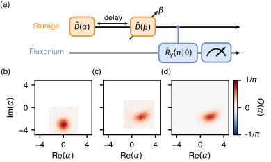
An alternative method to extract is through the time-evolution of the Husimi Q-function. By measuring the overlap between a displaced resonator state and , we can effectively construct the Q function, defined by
| (25) |
Measuring the Q function enables us to identify the Kerr nonlinearity by observing the evolution of the quantum state in phase space (Fig. 15(a)), where the Q function is given by
| (26) | |||
| (27) |
In Fig. 15(b), we prepared a coherent state with amplitude and immediately measured its Q function. As expected for a coherent state, the resulting Q function exhibits a Gaussian-shaped peak centered at in phase space. However, when we waited for before measuring the Q function, the state evolved under the Kerr interaction, leading to a shearing of the Q function distribution, as shown in Fig. 15(c). Photon loss during the evolution caused the Q function peak to shift inward from . We simulated the evolution using a master equation with the system parameters listed in Table 1, which successfully reproduces the data (Fig. 15(d)). The consistency between simulation and measurement provides additional validation of the Kerr nonlinearity extracted from the cavity Ramsey data.
Appendix E Wigner tomography and SNAP
E.1 Power Rabi calibration
This section outlines the power Rabi calibration procedure used for the Wigner tomography measurement. We performed Wigner tomography of the storage resonator by applying parity-selective measurements, where we drove the fluxonium at frequencies corresponding to even and odd photon number peaks, up to the 10th peak (Fig 4(a)). The difference between the measured qubit excitation probabilities after a prior resonator displacement yields the Wigner function. The drives can be described by
| (28) |
where is the duration of the Rabi pulse. We therefore need to perform a Rabi amplitude calibration at each photon-number-resolved peak by preparing a coherent state in the storage resonator and driving the fluxonium at the corresponding transition frequency (Fig. 16(a)). For the Wigner measurements, we used multiplexed Gaussian pulses to selectively address each peak. In Fig. 16(b), we show the Rabi calibration performed at the 0 peak, which exhibits a well-defined Rabi oscillation. However, for higher photon-number peaks, the calibration signal deviates from ideal Rabi oscillations and instead displays an overall rising trend with oscillatory features (Fig. 16(c)). We fitted the measured data using the master equation and extracted the qubit population associated with the neighboring photon-number states (Fig. 16(d)). The significant population in the and states during the pulse arises from the fact that the storage resonator undergoes substantial photon loss due to its limited relaxation time. The residual oscillations observed in the and populations suggest imperfect selectivity of the Rabi pulse, leading to weak off-resonant excitation of neighboring photon-number states. However, we could not use a longer Rabi pulse to improve selectivity due to the strong damping of the storage resonator. Consequently, the Wigner function we reconstruct deviates from the actual quantum state of the resonator. However, this deviation is well captured by our master equation simulation, as evidenced by the agreement between our simulation and experimental data in Fig. 4(c) and (d).
E.2 SNAP simulation and fidelity

| Loss mechanism | ||
|---|---|---|
| Intrinsic limit | ||
| Qubit initialization | ||
| Storage decay | ||
| Qubit depolarization | ||
| Qubit dephasing | ||
| Coherent errors |
Since the state preparation fidelity cannot be directly obtained from the overlap of the reconstructed Wigner function, we simulated the full SNAP process to evaluate the fidelity. The SNAP process was implemented by applying photon-number-selective pulses on the fluxonium, followed by a fast unconditional pulse. We used multiplexed Gaussian pulses for the selective pulses and a short Gaussian pulse for the fast unconditional pulse. The selective pulses were numerically optimized to suppress coherent errors, following the algorithm described in Ref. [44]. The drive pulses are described by
| (29) | |||
| (30) |
where and denote the durations of the slow and fast Rabi pulses, respectively. and are the optimized Fock-state-dependent amplitudes, frequencies, and phases of the selective drives, with . In Fig. 17, we show the Wigner functions of the ideal target state and the output state resulting from the simulated SNAP process, along with a center cut at . From the overlap of the Wigner functions, we extract a state preparation fidelity of 79% for the Fock state and 91% for the superposition state . The lower preparation fidelity of the Fock state arises from the larger displacement required to initialize the state, which results in increased photon loss during the SNAP sequence.
A more detailed breakdown of the loss mechanisms during the SNAP sequence is provided in Table 3. The intrinsic limit refers to the minimum infidelity achievable with our chosen displacement and SNAP parameters. To compute the contribution of each loss channel, we simulated the master equation while adding one loss channel at a time. The resulting contributions were then weighted and summed to account for the loss in addition to the intrinsic limit, using the following equation
| (31) |
Here, is the final weighted error reported for loss channel in Table 3. denotes the unweighted error contribution from a specific loss channel, is the total simulated preparation error, and is the intrinsic error associated with the finite fidelity of the chosen SNAP parameters. This rescaling accounts for the fact that the different loss channels are not strictly independent and ensures that the weighted sum of individual contributions matches the total observed additional error beyond the intrinsic limit. The coherent errors in the table are primarily attributed to phase accumulation during the nonselective pulse, which arises because the pulse is not resonant with all spectral peaks. However, the coherent errors could potentially be corrected with improved optimization algorithms or shorter unselective pulse.
Based on Table 3, aside from qubit initialization, the main sources of incoherent loss are storage decay and qubit dephasing during the selective pulse. Errors from qubit initialization could be addressed with improved active reset methods, whereas mitigating incoherent loss requires better-cohering qubit and resonator systems. To estimate the extent to which improved system coherence suppresses incoherent errors, we simulated the incoherent loss as a function of storage and qubit , as shown in Fig. 4(f). Since the unselective pulse is so short that it incurs essentially no incoherent loss, we only simulated the loss during the selective pulse. To simplify the simulation, we used representative parameters consistent with the experiment, choosing and . We also used pulse parameters identical to those in the experiment. We ran the master equation simulation while sweeping over the coherence times, and subtract out coherent errors to obtain the incoherent loss contribution.
References
- [1] D. Vitali, P. Tombesi, and G. J. Milburn, Quantum-state protection in cavities, Physical Review A 57, 4930 (1998).
- [2] D. Gottesman, A. Kitaev, and J. Preskill, Encoding a qubit in an oscillator, Physical Review A 64, 012310 (2001).
- [3] S. Zippilli, D. Vitali, P. Tombesi, and J.-M. Raimond, Scheme for decoherence control in microwave cavities, Physical Review A 67, 052101 (2003).
- [4] M. H. Michael, M. Silveri, R. T. Brierley, V. V. Albert, J. Salmilehto, L. Jiang, and S. M. Girvin, New Class of Quantum Error-Correcting Codes for a Bosonic Mode, Physical Review X 6, 031006 (2016).
- [5] W. Cai, Y. Ma, W. Wang, C.-L. Zou, and L. Sun, Bosonic quantum error correction codes in superconducting quantum circuits, Fundamental Research 1, 50 (2021).
- [6] W.-L. Ma, S. Puri, R. J. Schoelkopf, M. H. Devoret, S. Girvin, and L. Jiang, Quantum control of bosonic modes with superconducting circuits, Science Bulletin 66, 1789 (2021).
- [7] M. Reagor, W. Pfaff, C. Axline, R. W. Heeres, N. Ofek, K. Sliwa, E. Holland, C. Wang, J. Blumoff, K. Chou, M. J. Hatridge, L. Frunzio, M. H. Devoret, L. Jiang, and R. J. Schoelkopf, Quantum memory with millisecond coherence in circuit QED, Physical Review B 94, 014506 (2016).
- [8] S. Chakram, A. E. Oriani, R. K. Naik, A. V. Dixit, K. He, A. Agrawal, H. Kwon, and D. I. Schuster, Seamless High- Q Microwave Cavities for Multimode Circuit Quantum Electrodynamics, Physical Review Letters 127, 107701 (2021).
- [9] O. Milul, B. Guttel, U. Goldblatt, S. Hazanov, L. M. Joshi, D. Chausovsky, N. Kahn, E. Çiftyürek, F. Lafont, and S. Rosenblum, Superconducting Cavity Qubit with Tens of Milliseconds Single-Photon Coherence Time, PRX Quantum 4, 030336 (2023).
- [10] M. Reagor, H. Paik, G. Catelani, L. Sun, C. Axline, E. Holland, I. M. Pop, N. A. Masluk, T. Brecht, L. Frunzio, M. H. Devoret, L. Glazman, and R. J. Schoelkopf, Reaching 10 ms single photon lifetimes for superconducting aluminum cavities, Applied Physics Letters 102, 192604 (2013).
- [11] S. Rosenblum, P. Reinhold, M. Mirrahimi, L. Jiang, L. Frunzio, and R. J. Schoelkopf, Fault-tolerant detection of a quantum error, Science 361, 266 (2018).
- [12] J. Huang, T. J. DiNapoli, G. Rockwood, M. Yuan, P. Narasimhan, E. Gupta, M. Bal, F. Crisa, S. Garattoni, Y. Lu, L. Jiang, and S. Chakram, Fast Sideband Control of a Weakly Coupled Multimode Bosonic Memory (2025), arXiv:2503.10623 [quant-ph] .
- [13] C. K. Law and J. H. Eberly, Arbitrary Control of a Quantum Electromagnetic Field, Physical Review Letters 76, 1055 (1996).
- [14] S. Lloyd and S. L. Braunstein, Quantum Computation over Continuous Variables, Physical Review Letters 82, 1784 (1999).
- [15] M. Hofheinz, H. Wang, M. Ansmann, R. C. Bialczak, E. Lucero, M. Neeley, A. D. O’Connell, D. Sank, J. Wenner, J. M. Martinis, and A. N. Cleland, Synthesizing arbitrary quantum states in a superconducting resonator, Nature 459, 546 (2009).
- [16] S. Krastanov, V. V. Albert, C. Shen, C.-L. Zou, R. W. Heeres, B. Vlastakis, R. J. Schoelkopf, and L. Jiang, Universal control of an oscillator with dispersive coupling to a qubit, Physical Review A 92, 040303 (2015).
- [17] L. G. Lutterbach and L. Davidovich, Method for Direct Measurement of the Wigner Function in Cavity QED and Ion Traps, Physical Review Letters 78, 2547 (1997).
- [18] P. Bertet, A. Auffeves, P. Maioli, S. Osnaghi, T. Meunier, M. Brune, J. M. Raimond, and S. Haroche, Direct Measurement of the Wigner Function of a One-Photon Fock State in a Cavity, Physical Review Letters 89, 200402 (2002).
- [19] B. Vlastakis, G. Kirchmair, Z. Leghtas, S. E. Nigg, L. Frunzio, S. M. Girvin, M. Mirrahimi, M. H. Devoret, and R. J. Schoelkopf, Deterministically Encoding Quantum Information Using 100-Photon Schrodinger Cat States, Science 342, 607 (2013).
- [20] R. W. Heeres, P. Reinhold, N. Ofek, L. Frunzio, L. Jiang, M. H. Devoret, and R. J. Schoelkopf, Implementing a universal gate set on a logical qubit encoded in an oscillator, Nature Communications 8, 94 (2017).
- [21] S. Chakram, K. He, A. V. Dixit, A. E. Oriani, R. K. Naik, N. Leung, H. Kwon, W.-L. Ma, L. Jiang, and D. I. Schuster, Multimode photon blockade, Nature Physics 18, 879 (2022).
- [22] G. Kirchmair, B. Vlastakis, Z. Leghtas, S. E. Nigg, H. Paik, E. Ginossar, M. Mirrahimi, L. Frunzio, S. M. Girvin, and R. J. Schoelkopf, Observation of quantum state collapse and revival due to the single-photon Kerr effect, Nature 495, 205 (2013).
- [23] N. Ofek, A. Petrenko, R. Heeres, P. Reinhold, Z. Leghtas, B. Vlastakis, Y. Liu, L. Frunzio, S. M. Girvin, L. Jiang, M. Mirrahimi, M. H. Devoret, and R. J. Schoelkopf, Extending the lifetime of a quantum bit with error correction in superconducting circuits, Nature 536, 441 (2016).
- [24] J. M. Gertler, B. Baker, J. Li, S. Shirol, J. Koch, and C. Wang, Protecting a bosonic qubit with autonomous quantum error correction, Nature 590, 243 (2021).
- [25] V. V. Sivak, A. Eickbusch, B. Royer, S. Singh, I. Tsioutsios, S. Ganjam, A. Miano, B. L. Brock, A. Z. Ding, L. Frunzio, S. M. Girvin, R. J. Schoelkopf, and M. H. Devoret, Real-time quantum error correction beyond break-even, Nature 616, 50 (2023).
- [26] Z. Ni, S. Li, X. Deng, Y. Cai, L. Zhang, W. Wang, Z.-B. Yang, H. Yu, F. Yan, S. Liu, C.-L. Zou, L. Sun, S.-B. Zheng, Y. Xu, and D. Yu, Beating the break-even point with a discrete-variable-encoded logical qubit, Nature 616, 56 (2023).
- [27] R. Lescanne, M. Villiers, T. Peronnin, A. Sarlette, M. Delbecq, B. Huard, T. Kontos, M. Mirrahimi, and Z. Leghtas, Exponential suppression of bit-flips in a qubit encoded in an oscillator, Nature Physics 16, 509 (2020).
- [28] C. Berdou, A. Murani, U. Réglade, W. Smith, M. Villiers, J. Palomo, M. Rosticher, A. Denis, P. Morfin, M. Delbecq, T. Kontos, N. Pankratova, F. Rautschke, T. Peronnin, L.-A. Sellem, P. Rouchon, A. Sarlette, M. Mirrahimi, P. Campagne-Ibarcq, S. Jezouin, R. Lescanne, and Z. Leghtas, One Hundred Second Bit-Flip Time in a Two-Photon Dissipative Oscillator, PRX Quantum 4, 020350 (2023).
- [29] A. Eickbusch, V. Sivak, A. Z. Ding, S. S. Elder, S. R. Jha, J. Venkatraman, B. Royer, S. M. Girvin, R. J. Schoelkopf, and M. H. Devoret, Fast universal control of an oscillator with weak dispersive coupling to a qubit, Nature Physics 18, 1464 (2022).
- [30] H. Putterman, K. Noh, C. T. Hann, G. S. MacCabe, S. Aghaeimeibodi, R. N. Patel, M. Lee, W. M. Jones, H. Moradinejad, R. Rodriguez, N. Mahuli, J. Rose, J. C. Owens, H. Levine, E. Rosenfeld, P. Reinhold, L. Moncelsi, J. A. Alcid, N. Alidoust, P. Arrangoiz-Arriola, J. Barnett, P. Bienias, H. A. Carson, C. Chen, L. Chen, H. Chinkezian, E. M. Chisholm, M.-H. Chou, A. Clerk, A. Clifford, R. Cosmic, A. V. Curiel, E. Davis, L. DeLorenzo, J. M. D’Ewart, A. Diky, N. D’Souza, P. T. Dumitrescu, S. Eisenmann, E. Elkhouly, G. Evenbly, M. T. Fang, Y. Fang, M. J. Fling, W. Fon, G. Garcia, A. V. Gorshkov, J. A. Grant, M. J. Gray, S. Grimberg, A. L. Grimsmo, A. Haim, J. Hand, Y. He, M. Hernandez, D. Hover, J. S. C. Hung, M. Hunt, J. Iverson, I. Jarrige, J.-C. Jaskula, L. Jiang, M. Kalaee, R. Karabalin, P. J. Karalekas, A. J. Keller, A. Khalajhedayati, A. Kubica, H. Lee, C. Leroux, S. Lieu, V. Ly, K. V. Madrigal, G. Marcaud, G. McCabe, C. Miles, A. Milsted, J. Minguzzi, A. Mishra, B. Mukherjee, M. Naghiloo, E. Oblepias, G. Ortuno, J. Pagdilao, N. Pancotti, A. Panduro, JP. Paquette, M. Park, G. A. Peairs, D. Perello, E. C. Peterson, S. Ponte, J. Preskill, J. Qiao, G. Refael, R. Resnick, A. Retzker, O. A. Reyna, M. Runyan, C. A. Ryan, A. Sahmoud, E. Sanchez, R. Sanil, K. Sankar, Y. Sato, T. Scaffidi, S. Siavoshi, P. Sivarajah, T. Skogland, C.-J. Su, L. J. Swenson, S. M. Teo, A. Tomada, G. Torlai, E. A. Wollack, Y. Ye, J. A. Zerrudo, K. Zhang, F. G. S. L. Brandão, M. H. Matheny, and O. Painter, Hardware-efficient quantum error correction via concatenated bosonic qubits, Nature 638, 927 (2025).
- [31] A. Vrajitoarea, Z. Huang, P. Groszkowski, J. Koch, and A. A. Houck, Quantum control of an oscillator using a stimulated Josephson nonlinearity, Nature Physics 16, 211 (2020).
- [32] A. Grimm, N. E. Frattini, S. Puri, S. O. Mundhada, S. Touzard, M. Mirrahimi, S. M. Girvin, S. Shankar, and M. H. Devoret, Stabilization and operation of a Kerr-cat qubit, Nature 584, 205 (2020).
- [33] A. Z. Ding, B. L. Brock, A. Eickbusch, A. Koottandavida, N. E. Frattini, R. G. Cortinas, V. R. Joshi, S. J. de Graaf, B. J. Chapman, S. Ganjam, L. Frunzio, R. J. Schoelkopf, and M. H. Devoret, Quantum Control of an Oscillator with a Kerr-cat Qubit (2024), arXiv:2407.10940 [quant-ph] .
- [34] U. Réglade, A. Bocquet, R. Gautier, J. Cohen, A. Marquet, E. Albertinale, N. Pankratova, M. Hallén, F. Rautschke, L.-A. Sellem, P. Rouchon, A. Sarlette, M. Mirrahimi, P. Campagne-Ibarcq, R. Lescanne, S. Jezouin, and Z. Leghtas, Quantum control of a cat qubit with bit-flip times exceeding ten seconds, Nature 629, 778 (2024).
- [35] V. E. Manucharyan, J. Koch, L. I. Glazman, and M. H. Devoret, Fluxonium: Single Cooper-Pair Circuit Free of Charge Offsets, Science 326, 113 (2009).
- [36] A. Somoroff, Q. Ficheux, R. A. Mencia, H. Xiong, R. Kuzmin, and V. E. Manucharyan, Millisecond Coherence in a Superconducting Qubit, Physical Review Letters 130, 267001 (2023).
- [37] L. Ding, M. Hays, Y. Sung, B. Kannan, J. An, A. Di Paolo, A. H. Karamlou, T. M. Hazard, K. Azar, D. K. Kim, B. M. Niedzielski, A. Melville, M. E. Schwartz, J. L. Yoder, T. P. Orlando, S. Gustavsson, J. A. Grover, K. Serniak, and W. D. Oliver, High-fidelity, frequency-flexible two-qubit fluxonium gates with a transmon coupler, Physical Review X 13, 031035 (2023).
- [38] F. Wang, K. Lu, H. Zhan, L. Ma, F. Wu, H. Sun, H. Deng, Y. Bai, F. Bao, X. Chang, R. Gao, X. Gao, G. Gong, L. Hu, R. Hu, H. Ji, X. Ma, L. Mao, Z. Song, C. Tang, H. Wang, T. Wang, Z. Wang, T. Xia, H. Xu, Z. Zhan, G. Zhang, T. Zhou, M. Zhu, Q. Zhu, S. Zhu, X. Zhu, Y. Shi, H.-H. Zhao, and C. Deng, High coherence fluxonium manufactured with a wafer-scale uniformity process, Physical Review Applied 23, 044064 (2025).
- [39] D. Atanasova, I. Yang, T. Hönigl-Decrinis, D. Gusenkova, I. Pop, and G. Kirchmair, In Situ Tunable Interaction with an Invertible Sign between a Fluxonium and a Post Cavity, PRX Quantum 6, 020318 (2025).
- [40] G. Zhu, D. G. Ferguson, V. E. Manucharyan, and J. Koch, Circuit QED with fluxonium qubits: Theory of the dispersive regime, Physical Review B 87, 024510 (2013).
- [41] W. C. Smith, A. Kou, U. Vool, I. M. Pop, L. Frunzio, R. J. Schoelkopf, and M. H. Devoret, Quantization of inductively shunted superconducting circuits, Physical Review B 94, 144507 (2016).
- [42] D. I. Schuster, A. A. Houck, J. A. Schreier, A. Wallraff, J. M. Gambetta, A. Blais, L. Frunzio, J. Majer, B. Johnson, M. H. Devoret, S. M. Girvin, and R. J. Schoelkopf, Resolving photon number states in a superconducting circuit, Nature 445, 515 (2007).
- [43] R. W. Heeres, B. Vlastakis, E. Holland, S. Krastanov, V. V. Albert, L. Frunzio, L. Jiang, and R. J. Schoelkopf, Cavity state manipulation using photon-number selective phase gates, Physical Review Letters 115, 137002 (2015).
- [44] J. Landgraf, C. Flühmann, T. Fösel, F. Marquardt, and R. J. Schoelkopf, Fast quantum control of cavities using an improved protocol without coherent errors, Physical Review Letters 133, 260802 (2024).
- [45] G. Zheng, S. Lieu, E. L. Rosenfeld, K. Noh, and C. T. Hann, Cross-resonance control of an oscillator with an auxiliary fluxonium qubit, Physical Review Applied 23, 024067 (2025).
- [46] W. Pfaff, C. J. Axline, L. D. Burkhart, U. Vool, P. Reinhold, L. Frunzio, L. Jiang, M. H. Devoret, and R. J. Schoelkopf, Controlled release of multiphoton quantum states from a microwave cavity memory, Nature Physics 13, 882 (2017).
- [47] C. J. Axline, L. D. Burkhart, W. Pfaff, M. Zhang, K. Chou, P. Campagne-Ibarcq, P. Reinhold, L. Frunzio, S. M. Girvin, L. Jiang, M. H. Devoret, and R. J. Schoelkopf, On-demand quantum state transfer and entanglement between remote microwave cavity memories, Nature Physics 14, 705 (2018).
- [48] P. Campagne-Ibarcq, A. Eickbusch, S. Touzard, E. Zalys-Geller, N. E. Frattini, V. V. Sivak, P. Reinhold, S. Puri, S. Shankar, R. J. Schoelkopf, L. Frunzio, M. Mirrahimi, and M. H. Devoret, Quantum error correction of a qubit encoded in grid states of an oscillator, Nature 584, 368 (2020).
- [49] F. Valadares, N.-N. Huang, K. T. N. Chu, A. Dorogov, W. Chua, L. Kong, P. Song, and Y. Y. Gao, On-demand transposition across light-matter interaction regimes in bosonic cQED, Nature Communications 15, 5816 (2024).
- [50] W. Cai, X. Mu, W. Wang, J. Zhou, Y. Ma, X. Pan, Z. Hua, X. Liu, G. Xue, H. Yu, H. Wang, Y. Song, C.-L. Zou, and L. Sun, Protecting entanglement between logical qubits via quantum error correction, Nature Physics 20, 1022 (2024).
- [51] I. Yang, T. Agrenius, V. Usova, O. Romero-Isart, and G. Kirchmair, Hot Schrödinger cat states, Science Advances 11, eadr4492 (2025).
- [52] S. V. Lotkhov, S. A. Bogoslovsky, A. B. Zorin, and J. Niemeyer, Bridge-free technique for fabrication of submicron Al/AlOx/Al tunnel junctions for superconducting quantum circuits, Nanotechnology 22, 315302 (2011).
- [53] U. Vool, A. Kou, W. C. Smith, N. E. Frattini, K. Serniak, P. Reinhold, I. M. Pop, S. Shankar, L. Frunzio, S. M. Girvin, and M. H. Devoret, Driving forbidden transitions in the fluxonium artificial atom, Physical Review Applied 9, 054046 (2018).
- [54] H. Zhang, S. Chakram, T. Roy, N. Earnest, Y. Lu, Z. Huang, D. K. Weiss, J. Koch, and D. I. Schuster, Universal fast-flux control of a coherent, low-frequency qubit, Physical Review X 11, 011010 (2021).
- [55] T. Wang, F. Wu, F. Wang, X. Ma, G. Zhang, J. Chen, H. Deng, R. Gao, R. Hu, L. Ma, Z. Song, T. Xia, M. Ying, H. Zhan, H.-H. Zhao, and C. Deng, Efficient initialization of fluxonium qubits based on auxiliary energy levels, Physical Review Letters 132, 230601 (2024).
- [56] K. Nie, A. Bista, K. Chow, W. Pfaff, and A. Kou, Parametrically controlled microwave-photonic interface for the fluxonium, Physical Review Applied 22, 054021 (2024).
- [57] P. Groszkowski and J. Koch, Scqubits: A Python package for superconducting qubits, Quantum 5, 583 (2021).
- [58] S. P. Chitta, T. Zhao, Z. Huang, I. Mondragon-Shem, and J. Koch, Computer-aided quantization and numerical analysis of superconducting circuits, New Journal of Physics 24, 103020 (2022).
- [59] F. C. Binder, W. Ge, J. He, C. Lyu, M. A. C. Rossi, R. S. Coto, F. Minganti, O. Gerardo, T. Ball, X. Zhang, G. García-Pérez, S. Pirandola, M. Paternostro, S. Fux, Z. Leghtas, A. Clerk, A. Le Boité, R. Fazio, K. Murch, S. Hacohen-Gourgy, J. Combes, L. J. Fiderer, K. Brandner, A. Chenu, E. I. Chiacchio, X. Xu, S. Scopa, K. Snizhko, C. Arenz, P. Cappellaro, N. Lambert, F. Nori, and P. D. Nation, QuTiP: An open-source Python framework for the dynamics of open quantum systems, Quantum 7, 933 (2023).
- [60] A. Blais, A. L. Grimsmo, S. M. Girvin, and A. Wallraff, Circuit quantum electrodynamics, Reviews of Modern Physics 93, 025005 (2021).
- [61] J. Koch, T. M. Yu, J. Gambetta, A. A. Houck, D. I. Schuster, J. Majer, A. Blais, M. H. Devoret, S. M. Girvin, and R. J. Schoelkopf, Charge-insensitive qubit design derived from the Cooper pair box, Physical Review A 76, 042319 (2007).
- [62] J. A. Schreier, A. A. Houck, J. Koch, D. I. Schuster, B. R. Johnson, J. M. Chow, J. M. Gambetta, J. Majer, L. Frunzio, M. H. Devoret, S. M. Girvin, and R. J. Schoelkopf, Suppressing charge noise decoherence in superconducting charge qubits, Physical Review B 77, 180502(R) (2008).