CERN-TH-2025-101
FERMILAB-PUB-25-0344-T
INT-PUB-25-015
IPARCOS-UCM-25-029
KEK Preprint 2025-22
LTH 1403
MITP-25-037
UWThPh 2025-15
ZU-TH 37/25
The anomalous magnetic moment of the muon in the Standard Model: an update
Abstract
We present the current Standard Model (SM) prediction for the muon anomalous magnetic moment, , updating the first White Paper (WP20) Aoyama et al. [2020]. The pure QED and electroweak contributions have been further consolidated, while hadronic contributions continue to be responsible for the bulk of the uncertainty of the SM prediction. Significant progress has been achieved in the hadronic light-by-light scattering contribution using both the data-driven dispersive approach as well as lattice-QCD calculations, leading to a reduction of the uncertainty by almost a factor of two. The most important development since WP20 is the change in the estimate of the leading-order hadronic-vacuum-polarization (LO HVP) contribution. A new measurement of the cross section by CMD-3 has increased the tensions among data-driven dispersive evaluations of the LO HVP contribution to a level that makes it impossible to combine the results in a meaningful way. At the same time, the attainable precision of lattice-QCD calculations has increased substantially and allows for a consolidated lattice-QCD average of the LO HVP contribution with a precision of about 0.9%. Adopting the latter in this update has resulted in a major upward shift of the total SM prediction, which now reads (530 ppb). When compared against the current experimental average based on the E821 experiment and runs 1–6 of E989 at Fermilab, one finds , which implies that there is no tension between the SM and experiment at the current level of precision. The final precision of E989 (127 ppb) is the target of future efforts by the Theory Initiative. The resolution of the tensions among data-driven dispersive evaluations of the LO HVP contribution will be a key element in this endeavor.
We dedicate this paper to the memory of Simon Eidelman.
0 Executive summary
The experimental program to study the muon’s anomalous magnetic moment, , which started over sixty years ago at CERN, continues to inspire theoretical efforts to obtain a Standard-Model (SM) prediction with matching precision. In the SM, the dominant contributions to are due to QED corrections, followed by hadronic contributions (governed by QCD) and electroweak (EW) corrections. The CERN experiments provided tests of the Charpak et al. [1962] and Bailey et al. [1968] QED contributions and sensitivity to the leading-order (LO) hadronic corrections Bailey et al. [1979]. The BNL E821 experiment Bennett et al. [2006] reached a precision of 540 parts-per-billion (ppb), yielding sensitivity also to EW and higher-order hadronic contributions and intriguing tensions with the SM predictions available at that time. This provided motivation to launch the Fermilab E989 experiment, which started taking data in 2017, and has obtained measurements with increasing precision, from 460 ppb in 2021 Abi et al. [2021] to 200 ppb in 2023 Aguillard et al. [2023], all consistent with each other as well as with E821. The Fermilab experiment has just announced its final measurement result, with a precision of 127 ppb, and hence will enable, in principle, an exquisitely precise test of the SM.** * This paper was posted on arXiv on May 28, 2025. Sections 2, 3, 4, 5, 6, 7, and 8 and all numbers pertaining to the SM prediction have remained unchanged, but the experimental world average has been updated according to the E989 announcement on June 3, 2025 Aguillard et al. [2025], and the description in Secs. 0, 1, and 9 has been adapted accordingly. In particular, the experimental results in abstract, Table 1, Figs. 27, 40, and 83, and Sec. 9 have been updated. Meanwhile, a new experiment that will employ a largely different experimental method is currently under preparation at J-PARC Abe et al. [2019], allowing an independent cross-check of these results.
On the SM side, the QED and EW corrections are at less than 5 ppb already well quantified, while the notoriously difficult-to-calculate hadronic contributions are the dominant sources of theory error, rendering SM predictions of still considerably less precise than experiment. They, therefore, continue to be the main focus of the Muon Theory Initiative. A lot has happened regarding these corrections since the publication of the first White Paper (WP20) Aoyama et al. [2020].
The hadronic-vacuum-polarization (HVP) contribution was estimated in WP20 from hadronic cross-section data in the dispersive, data-driven method, while lattice-QCD methods were not mature enough to yield reliable results at the required precision. In the present review, we find that this situation is reversed. In the data-driven method, some tensions in the dominant channel were present in WP20 and were accounted for by inflating uncertainties. New cross-section measurements of the same channel that became available after WP20 have increased these tensions to a level that prevents forming any meaningful average for use in obtaining a precise and reliable evaluation of the HVP contribution. Moreover, at present no scientific grounds have been identified that would allow one to disregard any of the data sets relevant for the HVP evaluation.
Resolving the tensions in the hadronic cross-section data will require new analyses and measurements as well as an improved understanding of higher-order radiative corrections. Both are currently being pursued by several experiments and theorists. Despite the present difficult situation, a data-driven estimate of HVP remains an important goal of the Theory Initiative and an essential cornerstone on which to build future precise SM predictions. In this regard, also the -based HVP determination, which relies on consistent data sets, is being reconsidered in view of recent progress towards a model-independent evaluation of the required isospin-breaking corrections. While promising, this is still work in progress: the current status of a -based HVP estimate is reviewed here, but is not yet included in the overall evaluation.
On the other hand, thanks to dedicated efforts by the world-wide lattice field theory community, lattice-QCD calculations of HVP have matured considerably. The present review is informed by more than a dozen new papers (since WP20), which enable consolidated averages of (almost) all the components that are computed separately to construct the total LO HVP contribution in lattice QCD. The result is a reliable determination of the LO HVP contribution at precision that enters the SM prediction of . The change from a data-driven to a lattice-based estimate for the HVP contribution has resulted in a significant shift in the central value.
For the hadronic light-by-light (HLbL) contribution, significant progress since WP20 has been made in both the dispersive method and lattice QCD. On the data-driven side, improved calculations of short-distance constraints and a number of subleading contributions have become available, leading to a reduction of the uncertainty by about a factor of two compared to WP20. At the same time, new lattice-QCD calculations have reached a similar level of precision. The two averages, from phenomenology and lattice QCD, are combined into a final average with a precision below .
Table 1 gives a summary of the contributions to the SM prediction, along with the locations in this White Paper (WP25) where the results are discussed.
1 Introduction
The anomalous magnetic moment of the muon has been an enduring testbed of the SM and of its possible extensions (generically defined as beyond the SM, or BSM, physics). Both experiment and SM theory provide superb precision beyond parts-per-million (ppm), allowing one to put constraints on BSM physics through the comparison between the two. The Muon Theory Initiative (TI) was started in 2017 with the goal of bringing together the community of theorists and experimentalists working on this topic and of coordinating their efforts to provide a single, consensus number for the theoretical estimate of within the SM. The basis and the methodology behind such a number would be detailed in an extensive review, a so-called White Paper. The first edition was published in 2020 (WP20) Aoyama et al. [2020]. Since then, new measurements have been announced by the Fermilab experiment, the first result in 2021 Abi et al. [2021] with a precision of 460 ppb, and the second result in 2023 Aguillard et al. [2023] with 200 ppb. These new measurements are consistent with, but more precise than, the ones of the BNL experiment, and provide the basis of the current world average. The agreement of the two most precise experiments lends a high degree of reliability to this world average. The Fermilab E989 experiment has just announced its final results with the full set of all experimental data collected. Another experiment with a largely different experimental method is currently under preparation at J-PARC Abe et al. [2019], allowing an independent cross-check of these results.
For the physical interpretation of the muon experimental measurement, it is crucial to have a reliable SM prediction. Ideally, uncertainties on the SM prediction would be reduced to the same level as the experimental ones to maximize the BSM sensitivity. In the SM, is calculated from a perturbative expansion in the fine-structure constant . The most important contributions to this quantity arise from pure QED diagrams, but starting from order also hadronic contributions arise, in particular HVP and HLbL. Corrections due to EW bosons are small because of their large mass. They have been calculated at next-to-leading order (NLO) and are relevant at the present level of precision. The uncertainties are currently dominated by hadronic contributions due to the nonperturbative nature thereof, which make the corresponding theoretical calculations highly nontrivial. The goal of this second edition of the White Paper (WP25), as for the previous one, is to provide a detailed snapshot of the present situation and a new consensus SM number, before the final Fermilab result is announced.†† † This paper was posted on arXiv on May 28, 2025. Sections 2, 3, 4, 5, 6, 7, and 8 and all numbers pertaining to the SM prediction have remained unchanged, but the experimental world average has been updated according to the E989 announcement on June 3, 2025 Aguillard et al. [2025], and the description in Secs. 0, 1, and 9 has been adapted accordingly. In particular, the experimental results in abstract, Table 1, Figs. 27, 40, and 83, and Sec. 9 have been updated.
In recent years, the theoretical and experimental work aimed at reducing the uncertainties of the SM prediction has been particularly intense and relied on higher-order calculations, dispersive methods, lattice QCD, effective field theories, as well as new data inputs from experiments. For HLbL these efforts have indeed been successful and the change from WP20 to the present review is that the uncertainty has been reduced by about a factor of two. Concerning HVP the situation is more complicated as reflected by the fact that the present review does not present a number for a data-driven estimate of this contribution, since not yet understood discrepancies among different experiments have emerged. On the other hand, there has been significant progress in lattice-QCD calculations of this quantity, and the consensus number for the HVP contribution presented in this review is based on them. The change from a data-driven to a lattice estimate of this contribution also means that the central value has shifted, unfortunately, by more than the uncertainty quoted in WP20.
Activities of the initiative are coordinated by a Steering Committee that consists of theorists, experimentalists, and representatives from the Fermilab and J-PARC experiments. This committee also functions as the Advisory Committee for the workshops organized by the TI. Since the release of WP20, we organized four plenary workshops as well as focused mini-workshops. The format of the recent plenary workshops follows the previous editions with plenary sessions consisting of updates from experiments, updates from HVP and HLbL evaluations from dispersive approaches as well as lattice QCD. The plenary workshop in 2021 was held virtually during the period of the pandemic and was hosted by KEK Ple [2021]. After 2022, the three plenary workshops were held annually as in-person events in Edinburgh Ple [2022], Bern Ple [2023], and Tsukuba Ple [2024], respectively. The focused mini-workshops, held virtually, were devoted to high-precision calculations of HVP in lattice QCD Min [2020], the CMD-3 result for Min [2023a], Min [2023b], WP25 preparations prior to the Tsukuba workshop Min [2024], and the HVP evaluation from hadronic decays Min [2025]. At the next plenary workshop, planned to take place in Paris Ple [2025], the TI will discuss the next steps after WP25 toward reducing the theory errors to match the experimental precision. A summary of the prospects for such future improvements was compiled as contribution to the US Community Study on the Future of Particle Physics (Snowmass 2021) Colangelo et al. [2022a].
The Steering Committee is chaired by Aida El-Khadra, supported by Christoph Lehner and Michel Davier as co-chairs. Other committee members are‡‡ ‡ Simon Eidelman, a founding member of the Theory Initiative, served on the Steering Committee until he passed away in June 2021. Gilberto Colangelo, Martin Hoferichter, Laurent Lellouch, Tsutomu Mibe, Lee Roberts, Thomas Teubner, and Hartmut Wittig. The Steering Committee’s roles are the long-term planning of the Theory Initiative, the organization of the workshops, and the coordination of writing the White Paper and its updates. This review (WP25) has kept the same structure as the previous one and is organized in four main chapters, namely data-driven HVP, lattice HVP, analytic HLbL, and lattice HLbL, the writing of which was delegated to four corresponding working groups. The coordinators of the working groups are:
- •
Data-driven HVP: Vincenzo Cirigliano, Achim Denig, Fedor Ignatov, Bogdan Malaescu
- •
Lattice HVP: Steven Gottlieb, Antonin Portelli
- •
Analytic HLbL: Johan (Hans) Bijnens, Anton Rebhan
- •
Lattice HLbL: Luchang Jin, Harvey Meyer
In addition, sections on the QED and EW contributions are coordinated by Makiko Nio and Dominik Stöckinger, respectively.
This paper was written under the following agreements within the initiative. All participants of the past workshops, members of working groups, and their collaborators were invited to become co-authors of WP25. Essential input papers that were accepted for publication by May 22, 2025 were fully considered and included in the averages, while brief descriptions of unpublished papers available on arXiv before Apr 22, 2025 are also included.
The rest of the review is organized as follows: we first discuss the evaluations of data-driven HVP calculations in Sec. 2 and lattice-QCD calculations in Sec. 3, followed by comparisons between them in Sec. 4. Then, we describe evaluations of HLbL by using data-driven and analytic approaches in Sec. 5, and lattice QCD in Sec. 6. Lastly, QED and EW contributions are given in Secs. 7 and 8, respectively. We summarize the conclusions and outlook for the current SM prediction in Sec. 9.
2 Data-driven calculations of HVP
R. Aliberti, G. Benton, D. Boito, M. Bruno, C. M. Carloni Calame, V. Cirigliano, G. Colangelo, L. Cotrozzi, M. Cottini, M. Davier, A. Denig, V. Druzhinin, M. Golterman, A. Hoecker, M. Hoferichter, B.-L. Hoid, S. Holz, F. Ignatov, A. Keshavarzi, B. Kubis, A. Kupich, S. Laporta, T. Leplumey, Q. Liu, I. Logashenko, G. López Castro, A.-M. Lutz, B. Malaescu, K. Maltman, A. Miranda, S. E. Müller, A. Nesterenko, D. Nomura, M. Passera, S. Peris, F. Piccinini, R. Pilato, L. Polat, P. Roig, J. Ruiz de Elvira, A. Signer, P. Stoffer, T. Teubner, G. Toledo, Y. Ulrich, G. Venanzoni, A. Wright, E. Zaid, Z. Zhang
2.1 Introduction
The calculation of the LO HVP contribution in terms of hadronic cross sections proceeds via the master formula Bouchiat and Michel [1961], Brodsky and de Rafael [1968], Lautrup and de Rafael [1968], Gourdin and de Rafael [1969]
| (2.1) |
with muon mass , fine-structure constant , and kernel function
| (2.2) |
Here, the hadronic -ratio,
| (2.3) |
is defined photon-inclusively, so that the integration starts at the threshold due to the channel. The challenge in evaluating at sub-percent level thus lies in the extraordinary precision requirements for the measurement of cross sections, especially, for the crucial channel. In this section, various aspects of this program are discussed, including reports from the experiments (Sec. 2.2), indirect cross-section measurements via decays (Sec. 2.3), Monte-Carlo (MC) tools (Sec. 2.4), global data combinations (Sec. 2.5), theory developments (Secs. 2.6, 2.7, and 2.8), higher orders (Sec. 2.9), and the MUonE project (Sec. 2.10). A summary of the current situation together with an outlook to future prospects is provided in Secs. 2.11 and 2.12.
Throughout, in addition to the total LO HVP contribution as defined in Eq. 2.1, also so-called Euclidean-window observables will be considered. First introduced by RBC/UKQCD Blum et al. [2018], weight functions in Euclidean time are introduced that separate the entire integral into a short-distance (SD), intermediate (W), and long-distance (LD) component, see Sec. 3.4 for the precise definitions. Importantly, as detailed in Sec. 4.1, these weight functions can be translated into center-of-mass (CM) energy , to be inserted into Eq. 2.1, so that data-driven evaluations of the same quantities become possible, a connection that is addressed in more detail in Sec. 4.
2.2 Status and perspectives of experiments
2.2.1 CMD-3
The CMD-3 Aulchenko et al. [2001], Khazin [2008] and SND Achasov et al. [2009] experiments have been in operation at the electron–positron collider VEPP-2000 Shatunov et al. [2016], Shwartz et al. [2016] since 2010. The collider provides an instantaneous luminosity of up to at the maximum CM energy , a world record for single-bunch luminosity. Overall, more than 1 fb-1 of data has already been collected by each experiment across the entire available CM energy range from 0.32 to 2.007 GeV. Today, VEPP-2000 is the only collider operating at these energies.
The new generation CMD-3 detector was designed and constructed with a major upgrade of all subsystems compared to its predecessor CMD-2 experiment. In particular, a new drift chamber provided higher efficiency and more than twice better momentum resolution, and a new liquid-xenon (LXe) calorimeter added multi-layer tracking capabilities and shower profile measurement. The detector also has completely new up-to-date electronics and an elaborate trigger system. The main goals of experiments at VEPP-2000 include the high-precision measurement of cross sections of various modes of at low energies. All major channels are under analysis with final states of up to 7 pions, or two kaons and three pions Ignatov et al. [2019]. Many results have already been published by CMD-3 as shown in Fig. 1(left), where Akhmetshin et al. [2020], Akhmetshin et al. [2023], and Ignatov et al. [2024a], Ignatov et al. [2024b] have appeared since WP20, and many more channels are still being analyzed.
The most crucial channel for evaluation of is the simplest production. The study of this process has a long history since the first colliders, with numerous experiments that have contributed over the years, as shown in Fig. 1(right). This enormous effort is still not sufficient; to match the expected precision of the experiments, this channel should be known with a precision better than 0.2%. The latest, and one of the most precise measurements, was provided by the CMD-3 experiment Ignatov et al. [2024a], Ignatov et al. [2024b]. This new measurement was intensely scrutinized and reviewed by the community within a specially organized series of seminars Min [2023a], Min [2023b], where a comprehensive list of questions covering all aspects of the analysis was asked by a panel of experts nominated by the TI Steering Committee. No pitfalls were found.
The CMD-3 analysis is based on the largest ever data set of selected events at , which is an order of magnitude larger statistics compared to most of the previous measurements. The large statistics were crucial to study various systematic effects in detail and to obtain a sharper view of possible detector effects. It would be impossible to apply the analysis procedure, developed for the CMD-3 measurement, to the data collected by the predecessor CMD-2 experiment, as many of the systematic effects would be hidden under statistical fluctuations. The estimation of the possible systematic effects in the CMD-3 analysis is done in the most conservative way, with the goal to achieve a high confidence in the final declared precision even at the expense of possible increase in error.
One of the key features of the analysis, in contrast to other measurements, is the use of three independent sources of information for measuring the number of detected events: using momentum distributions of two particles measured in the tracking system, using detected energy depositions in the LXe calorimeter, or using the polar angular distribution. All three methods are consistent within 0.2%.
Another important aspect of the performed analysis by CMD-3 was a comprehensive study of the detector acceptance systematic uncertainty due to the determination of the polar angle. As a by-product of this investigation, the forward–backward charge asymmetry of was measured with an integrated statistical precision of about 0.025%. A strong 1% deviation was observed from the prediction based on the conventional scalar QED (sQED) approach used for the calculation of radiative corrections, as shown in Fig. 2(left), which was never noted before. The improved generalized-vector-meson-dominance (GVMD) model was proposed in Ref. Ignatov and Lee [2022], which gives remarkable agreement with the experimental data. This was later confirmed by a calculation in the dispersive formalism Colangelo et al. [2022b], see Sec. 2.7.4. At first the dispersive approach prediction still displayed some visible deviation from the data, but a subsequent identification of an incorrect treatment of endpoint singularities in the dispersive calculation integrals led to an astonishing consistency with the experimental asymmetry and the GVMD prediction, see Refs. Budassi et al. [2025], Colangelo et al. [2022b] and Figs. 2 and 23. Independent beyond-sQED calculations within the GVMD and the dispersive formalism were also performed in Ref. Budassi et al. [2025], and some of the cross-checks were facilitated by the RadioMonteCarLow 2 effort, see Sec. 2.4. The observed limitation of the sQED approach also suggests to revisit the radiative corrections used in the initial-state-radiation (ISR) measurements, where this can contribute to the -even two-photon-exchange corrections and consequently affect the experimental extraction of the pion vector form factor (VFF) , see Refs. Abbiendi et al. [2022], Aliberti et al. [2025]. The dispersive approach offers a more comprehensive description of the pion VFF, as it incorporates the correct analytic properties by construction. However, the GVMD model can provide a much simpler framework for more complicated calculations involving additional hard photons, and it also allows for iterative refinement of the VFF through the inclusion of additional terms. Ideally, having both calculations available would be beneficial for cross-checks.
The dominant systematic contribution in the CMD-3 measurement comes from the fiducial-volume determination and was conservatively estimated as 0.5%/0.8% (RHO2018/2013) as shown in the summary systematic Table 2 of Ref. Ignatov et al. [2024b]. The achieved consistency at the permil level in the measured asymmetries of , processes in CMD-3 together with overall stability of the result over different detector regions gives a quite confident level of control of this source of systematics. Such a cross-check with the extracted pion VFF within the different polar angle selections is shown in Fig. 2(right). For comparison, dashed lines show how the experimental points should look like in case of the presence of a 0.5% systematic effect from the fiducial volume in the measured cross section due to the most natural scenarios, either by a miscalibrated -scale of the detector or by a constant bias of the reconstructed polar angle for tracks of one of the charges. It is seen that the data is about 5 times more consistent than the declared assigned systematics. It should also be noted that some other previous measurements, which showed the dependence of results versus the detection polar angle, demonstrated variations an order of magnitude larger than those achieved by CMD-3.
Another important test was the measurement of cross section, predicted by QED. It was done for the momentum-based analysis for only, where the momentum resolution of the tracking system allowed to separate muons from other particles. The observed average ratio of the measured cross section to the QED prediction proves the consistency of most parts of the analysis procedure, including the separation procedure, detector effects, evaluation of radiative corrections, etc.
Reaching improved precision requires support by MC tools. One of the drawbacks of the CMD-3 analysis was that only one generator, MCGPJ, with the required precision was available for the process. Since the CMD-3 publication, the Pavia group presented a calculation of the hadronic channel at NLO matched to a parton shower algorithm, with implementation in the new version of the BabaYaga@NLO MC event generator Budassi et al. [2025]. The values of integrated radiative corrections and the forward–backward charge asymmetry in were confirmed. The strong RadioMonteCarLow 2 community effort, going towards next-to-next-to-leading-order (NNLO) precision and above, will help further clarify and strengthen the theoretical side of the experimental measurements, as discussed in Sec. 2.4. This effort will be mandatory if there is a wish to reach permil-level experimental precision in this channel. This aspect is even more critical for the ISR measurements right now, as the LO of the ISR processes starts at NLO precision of MC tools for the energy-scan experiments.
The total systematic precision of the CMD-3 measurement was conservatively estimated as 0.7% in the central region near the resonance. It is important to give a dedicated clarification regarding the treatment of the provided experimental systematic uncertainties. Being dominated mainly by a single source, the CMD-3 publication provides only the total systematic error for each point and suggests using a single-source full systematic covariance matrix accordingly, for simplicity of further external use. This yields an even more conservative evaluation of the uncertainty of the integral compared to splitting over different statistically independent systematic contributions. Such a prescription in the case of direct point-by-point integration conventionally assumes using 100% correlated systematic uncertainty. However, strictly speaking, the exact energy dependence of the required systematic corrections are unknown. Therefore, it is essential to consider the uncertainties of the uncertainty, as argued in Sec. 2.3.6 of WP20. This is especially important given the reached advancements in statistical precision and the entirely dominant systematic uncertainties of the latest CMD-3 measurement. A strict interpretation of the provided systematic error values is that they accommodate an underlying systematic effect with possible internal correlations up to 100%. Furthermore, these values allow for any energy-dependent functional form of the required systematic correction, provided it remains within the specified systematic band. This prescription was commonly assumed by experimentalists in most of the measurements and for most of the separate systematics sources (even when a correlation matrix was provided). Applications that exploit correlations between data and consider only 100% strict correlation from the first to the last energy point of different split systematic contributions can produce a significant underestimate of the uncertainty on the quantity being evaluated. This, for example, applies to the all analyticity-constrained fits described in Sec. 2.6, where using only “100% correlated systematic” of each separate source strongly reduces the degrees of freedom of the fit and consequently shrinks the systematic part of errors from that. Such an underestimation of the systematic error of the evaluated integrals may in some cases be greater than a factor 1.5, as shown in Ref. Leplumey and Stoffer [2025] and noted in Sec. 2.6.1 for the CMD-3 data treatment case.
The published CMD-3 pion VFF result was based on the full data sample collected at energies below 1 GeV before 2024 (62 pb-1) and on a small subset of data, about 24 pb-1, collected at energies above 1 GeV. The full data sample above 1 GeV is under analysis. The preliminary results on the pion VFF were obtained for data collected in 2019–2021 (about 170 pb-1). The major data sample of 580 pb-1 was collected in 2022 and 2023; these data are yet to be incorporated into the ongoing analysis. Data analysis at these CM energies differs from the one implemented in Ref. Ignatov et al. [2024b]:
- •
The momentum resolution of the CMD-3 tracking system does not allow one to distinguish momenta of , , and in , , and , correspondingly. Thus, the final-state identification is based on the analysis of energy deposition in the calorimeter. In order to cross-check the identification procedures, two independent methods are being developed—one is based on data from the LXe calorimeter only (similar to the method described in Ref. Ignatov et al. [2024b]) and another is based on the data from the full calorimeter and machine learning. Muons and pions cannot be robustly distinguished by the CMD-3 calorimeter response, thus the number of pairs is evaluated from the number of detected . The identification procedure based on the analysis of angular distributions is statistically limited and is applied only as an overall cross-check, not point-by-point.
- •
At energies above 1 GeV, the cross section for the 2 final state drops, but it rises for many other hadronic final states, most notably for . In order to keep background low, strict selection cuts are used, which introduces larger efficiency corrections, which differ for , , and .
New data taking at energies below 1 GeV started in 2024 and is expected to continue through 2025 with the goal to scan the whole CM energy range from 0.32 to 1 GeV and to collect 2–3 times more data compared to previous scans. The CMD-3 result Ignatov et al. [2024b] is systematically limited. Nevertheless, the gain in statistics will be beneficial for the pion VFF measurement as well, as it will open additional possibilities for the systematics studies. It should be noted that a significant bulk of the data collected (and planned to be collected) in 2024/2025 is taken with the directions of and beams reversed; that allows one to cross-check various detector-specific efficiency corrections.
The luminosity provided by VEPP-2000 at energies allows for statistical accuracy of (0.1–0.2)% for the pion VFF. Such precision is required in order to match the accuracy of the evaluation in the dispersive approach to the precision of the final FNAL result. Reduction of the systematic uncertainty to the same level requires a significant upgrade of the CMD-3 detector. The key directions of the upgrade are: a new tracking system with improved momentum resolution; the possibility for the precise and robust measurement of the polar angles of the tracks and the position of the vertex along the beam axis; a dedicated system to study nuclear interactions of pions with the material of the beam pipe and the tracking system. The upgrades are being designed. It is estimated that the data taking with the upgraded detector can start around 2030. It should be mentioned that 0.1% precision for the pion VFF also sets very high requirements for the theoretical models and corresponding MC codes used to evaluate the radiative corrections.
The same data sets discussed here are used for the measurement of cross sections of many exclusive channels of beyond . The second most important channel after for the evaluation is . The first result for this channel was published as a by-product of the measurement Ignatov et al. [2024b], based on the small subset of identified as a background to . A dedicated analysis of the full data set is in progress and is expected to be released in 2025.
2.2.2 SND
Since 2020 several hadronic cross sections were measured at the SND experiment at the VEPP-2000 collider. A precise measurement of the cross section was carried out in the vicinity of the meson resonance Achasov et al. [2024a]. The systematic uncertainty in the measured cross section at the maximum of the resonance is 0.9%. The cross section was measured in the energy range Achasov et al. [2024b]. The SND result is consistent with the previous BaBar measurement Lees et al. [2021a], but is more accurate. The SND data on the cross section below 2 GeV Achasov et al. [2020a] are also in reasonable agreement with the BaBar measurement Aubert et al. [2008]. The process was studied in the energy range from threshold up to 2 GeV. The measured cross section Achasov et al. [2022a], Achasov et al. [2023a], Achasov et al. [2024c] is presented in Fig. 3(left). New data on the processes with multiphoton final state Achasov et al. [2020b], Achasov et al. [2022b], Achasov et al. [2023b], Achasov et al. [2024d] were obtained.
Currently, the SND collaboration works with and channels in the and energy regions, respectively, using 69 pb-1 data. They have faced serious challenges due to the fact that detector performance was very inconsistent during the 2017–2018 experiment. Despite these problems, it is possible to perform high-precision measurements of the cross section, using a modified version of the reconstruction software. A new algorithm of / separation allows one to suppress background by a factor of in the whole energy region, thus limiting the growth of the systematic error with decrease of . An improved reconstruction algorithm allows one to reduce the number of poorly reconstructed tracks. Simulated events now better describe experimental inefficiencies of the cosmic veto and energy-deposition cut, after introduction of the light quenching effects in the plastic scintillator of the muon system and NaI(Tl) of the electromagnetic (EM) calorimeter. The current number of the selected events makes the statistical uncertainty negligible compared to the systematic one. Due to the increased tensions between the most precise measurements of the cross section, a blinding procedure was introduced for the earlier stages of the SND analysis. The efficiency of was modified via multiplying it by , where and are randomly generated parameters, unknown to the researchers. The preliminary results of the unblinded cross-section measurement are shown in Fig. 3(right). Current estimates of the systematic uncertainty are (0.6–0.8)% in the whole energy range, due to much higher statistics and improvements in the simulation and reconstruction algorithms, compared to the 2020 SND analysis. Progress with the channel was delayed, since this analysis relies on the high-precision measurements of the integrated luminosity from the analysis. Preliminary estimates of the systematic uncertainty of cross-section measurements show it to be no greater than 1.4%.
2.2.3 KLOE
The KLOE experiment took data during 2001–2006, with a total integrated luminosity of 2.5 at (the peak) and 250 off-peak at (in 2006). Peak luminosity was reached during the 2005 run with a luminosity of 8.5 /day. KLOE has published three precise cross-section measurements of : KLOE08 Ambrosino et al. [2009], KLOE10 Ambrosino et al. [2011], and KLOE12 Babusci et al. [2013a], which have been used for the evaluation of the 2 contribution to Aoyama et al. [2020]. The KLOE08 and KLOE12 analyses were performed with a small-angle (SA) selection where the photon is required to be within or (i.e., missing momentum) resulting in 240 ( 3.5 million events) of data taken in 2002. The KLOE10 analysis was performed on 232 from 2006 (corresponding to 0.6 million events), after the photon polar angle is selected at large angle (LA), i.e., . Further details of the analyses can be found in Refs. Aoyama et al. [2020], Aliberti et al. [2025], Venanzoni [2018], and details on the agreement and combination of the three results are found in Ref. Anastasi et al. [2018].
In the KLOE08, KLOE10, and KLOE12 analyses, the MC generator Phokhara (version 5) was used, including NLO ISR, final-state-radiation (FSR) corrections, and simultaneous emission of one ISR and one FSR photon Czyż et al. [2020], Müller [2023]. Phokhara was interfaced with the standard KLOE MC GEANFI to compute MC efficiencies as a function of the reconstructed , and to compute the radiator function used to relate the measured differential cross section for to the cross section . In addition, Phokhara was used to correct for the shift between the measured and the invariant mass of the intermediate photons for FSR events. The FSR treatment was done assuming point-like pions (FsQED, see Ref. Aliberti et al. [2025] for definitions).
The KLOE12 analysis normalized the cross section using a cross-section measurement with the photon at SA. The error quoted by the authors of Phokhara on the ISR part of the generator is 0.5%, this error cancels out in the extraction of the pion VFF from the ratio. In the KLOE12 analysis, a global uncertainty of 0.2% was estimated for the factorization approximation when subtracting FSR for muons, and for the correction due to the FSR shift for pions. The effects of additional diagrams not present in Phokhara (v5) for muons was estimated to be 0.1% at most. The SA selection greatly suppresses events with only one hard photon from FSR and no ISR, as well as a large part of events with one photon from ISR and one from FSR. For KLOE08, the uncertainty due to the treatment of FSR events is estimated to be 0.3%. For KLOE10, the uncertainty on the treatment of FSR has been estimated to be 0.5% due to the uncertainty of the pion VFF at and 0.6% due to a comparison of FSR modeled with SU(3) chiral perturbation theory (ChPT) Aliberti et al. [2025], Gasser and Leutwyler [1984] with respect to the treatment used in Phokhara.
Within the RadioMonteCarLow 2 efforts Aliberti et al. [2025], “tuned comparisons” (see Ref. Actis et al. [2010] for the definition) between Phokhara 10.0§§ § Differences between Phokhara5 (which was used by KLOE) and Phokhara10 have been investigated in Ref. Campanario et al. [2019]. (which has a full NLO matrix element for and final state) and other MC generators—namely, AfkQed, BabaYaga@NLO, KKMC, and McMule, all described in Ref. Aliberti et al. [2025]—were performed Venanzoni [2024], Aliberti et al. [2025], in order to investigate radiative correction effects both due to missing NNLO contributions in Phokhara and also to test the validity of the generator at NLO, as questioned in Ref. Davier et al. [2024a]. The following configurations have been studied:
- •
before and after SA angular acceptance, considering both ISR and FSR emission;
- •
before and after SA and LA angular acceptance for only ISR emission—due to limitations of other MC generators used in this comparison Venanzoni [2024]. In the case of LA acceptance, it was also possible to compare AfkQed vs. Phokhara after the trackmass cut;¶¶ ¶ The trackmass is a kinematic variable defined in Ref. Ambrosino et al. [2009]. The tails in its distribution are mainly due to radiative corrections, therefore, it is sensitive to (N)NLO effects. this was not possible in the case of SA due to the AfkQed limitations for the KLOE configuration.
In this study, the and cross sections as a function of the invariant mass of the two pions and muons from Phokhara were compared with the predictions from other generators Venanzoni [2018], Aliberti et al. [2025]. Vacuum polarization (VP) was switched off and detector effects (involving smearing of momenta) were not included. The selection cuts used for the SA and LA comparisons are described in Ref. Aliberti et al. [2025], in the sections “KLOE-like small-angle scenario” and “KLOE-like large-angle scenario,” respectively.
The studies on muons showed good agreement with the SA acceptance between Phokhara, McMule, and KKMC, with a difference below between Phokhara and KKMC for most of the spectrum, as shown in Fig. 4. We note, see Fig. 32 of Ref. Aliberti et al. [2025], that this is not the case for the so-called “-scenario” where differences between generators (particularly KKMC and AfkQed) reach a few percent at . In the inclusive selection (i.e., without angular acceptance cuts), there are known differences for between Phokhara and KKMC Jadach [2005], up to , due to missing exponentiation in Phokhara, but with negligible effects on (in the pion case)—which is dominated by the low-energy region.
The studies on pions showed excellent agreement between Phokhara and McMule in the inclusive and SA Venanzoni [2024] and LA acceptance selections, see Fig. 5(left). This is good confirmation of the correctness of the implementation of full NLO matrix elements in Phokhara. The LA acceptance selection (KLOE10) was studied also after the trackmass cut, see Fig. 5(right), which is sensitive to (N)NLO effects. With acceptance cuts only, an agreement below 0.5% was found around the peak () between Phokhara and AfkQed. With an additional cut on the trackmass variable on top of acceptance cuts, the agreement at the peak was found to be below 1%, as shown in Fig. 5(right). The larger differences observed below are expected to originate from the different treatment of radiative corrections. While the size of the differences is still within the systematic uncertainty of KLOE10 Ambrosino et al. [2011], see Fig. 5(right), for the future analyses this difference is a further indication of the need for a NNLO MC generator, on which work is in progress Aliberti et al. [2025].
Preliminary results, which do not yet account for realistic detector effects, indicate the following:
- •
Phokhara shows excellent agreement with McMule for and . These results confirm the correct implementation of NLO matrix elements in Phokhara and exclude possible issues associated with Phokhara as questioned in scenario 1 of Ref. Davier et al. [2024a].
- •
For , the agreement between Phokhara and KKMC is mostly within for ISR, ISR+FSR in both inclusive and SA selections, before the trackmass selection is applied. Differences above GeV2 (in ), reaching up to approximately are due to missing exponentiation in Phokhara (and have negligible effects on in the pion case). Work is currently in progress to estimate the effects of radiative corrections due to the trackmass cut on muons, which can be sensitive to the presence of additional photon emission.
- •
For a comparison with AfkQed in the LA selection reveals differences below 0.5% when considering acceptance cuts, and below when including also the trackmass cut, at the peak. These findings limit the impact of NNLO effects on the LA analysis (KLOE10) as possible explanation for the discrepancy with BaBar and CMD-3 experiments.
More studies are in progress, specifically: enlarging the statistics; including realistic detector effects (GEANFI); including more refined hadron–photon models for FSR (beyond FsQED) Aliberti et al. [2025] and ISR NNLO radiative corrections; and applying the trackmass selection for SA (KLOE08) and (KLOE12) analyses.
A new SA KLOE 2 analysis on 2004–2005 data, normalized to , has started with the aim of clarifying the current tension with respect to other HVP evaluations. It is based on 25 million events, corresponding to times the statistics of the KLOE published analyses, which have not yet been analyzed. The 2006 off-peak data will also be used for additional cross-checks and systematic studies. This new analysis, called KLOE-nxt, will employ new software tools and additional validation tests aiming to a precision of 0.4% on the contribution to , representing a two-fold improvement in accuracy compared to the previous KLOE12 result Zaid [2024]. It will also benefit from the ongoing work towards a NNLO implementation of Phokhara Aliberti et al. [2025]. KLOE-nxt will provide an important cross-check of the published results and will be conducted in a blinded manner Punzi [2023].
In addition, KLOE is analyzing the three-pion cross section using the radiative-return method with 1.7 fb-1 of data collected at the meson mass Cao and Kang [2020].
2.2.4 BaBar
A number of hadronic processes have been studied by BaBar since WP20, including Lees et al. [2021b] and Lees et al. [2021c] in 2021, as well as Lees et al. [2023a] in 2022. In particular, the cross section, which represents the second largest input of the HVP contribution to , was measured in 2021 Lees et al. [2021a] using 469 of data collected by the experiment near the resonance, with CM energies ranging from 0.62 to 3.5 GeV via the ISR method. The analysis requires all final-state particles to be detected, namely two good-quality opposite-sign charged tracks and at least three photons, one being the ISR candidate with a CM energy larger than 3 GeV while the remaining photons must form one or more candidates with invariant masses GeV. A kinematic fit is performed on selected events and provides a quality value used to reject background processes, estimated with MC simulation. The cross section is studied separately below and above 1.1 GeV because of the detector resolution which significantly distorts the mass spectrum in the lower region. From threshold to 2.0 GeV, the measured HVP contribution of this channel is , with a systematic uncertainty of 1.3% near the and resonances, dominated by the detection efficiency, radiative correction, and luminosity. This result improves the precision by a factor of about 2 compared to calculations based on previous analyses.
The last BaBar analysis to measure the cross section was published in 2009 and 2012 Aubert et al. [2009a], Lees et al. [2012] with around half the BaBar statistics. To cancel out the ISR photon efficiency and the VP, the measured mass spectrum is divided by the spectrum, equivalent to the ratio of each final state’s bare cross section. The separation between pions and muons was based on particle identification (PID) which required both charged tracks to have momenta larger than 1 GeV in order to make the muon identification more reliable. PID was found to be the dominant source of systematic uncertainties on the prediction, with a total relative systematic error of 0.5% for energies from 0.5 to 1 GeV.
An upcoming BaBar analysis, intended to be published in 2025, aims at improving the precision on the HVP contribution to from . For that purpose, the entirety of BaBar data will be studied, while PID requirements on the tracks will be removed. An angular fit is considered as a new method Davier [2017] to distinguish the main signal (, ) and remaining background (, ) processes, based on the cosine of the angle between the negative charge track and the ISR photon in the 2-track CM frame. To further differentiate the shapes of the dipion and dimuon distributions, the track momentum selection required in the previous analysis is released, increasing the statistics at the same time. Overall, this new study will result in an independent measurement of the cross section.
A first step towards this objective was taken with a study of additional radiation in ISR processes, published in 2023 Lees et al. [2023b] and relying on all the data collected by BaBar. The intent was to evaluate how accurate the Phokhara and AfkQed generators are in simulating data and to measure the relative proportions of additional radiations in and processes with ISR, at “LO” (no additional photon), “NLO” ( real photon), and “NNLO” ( real photons, simulated only by AfkQed). Tracks are assumed to have pion masses, while dipion and dimuon events are identified according to tight PID selections. Kinematic fits are performed on events according to the different configurations in which additional photons are emitted. In the case of “NLO” events, two fits are applied depending on whether the single additional photon is detected in the EM calorimeter at a large angle (LA) from the beams, between 0.35 and 2.4 radians, or it is emitted at a small angle (SA), assumed to be collinear with the beams. For “NNLO” events, three fits are devised considering the two additional photons can both make large angles (2LA), small angles (2SA), or one of each configuration (LA+SA).
Inputs to the fits are the measured energy and direction of the ISR photon, the momenta and angles of both charged tracks, as well as the measured energy and angles of detected additional photons in the LA fit. Returned quantities are values and fit kinematic variables. Events are classified depending on the smallest , with the additional requirement that fit energies are larger than 200 MeV either in the laboratory frame for LA photons or in the CM frame for SA photons. Events below these thresholds are classified as “LO.”
The distinction between “NLO” LA radiations from ISR and FSR is performed by fitting the distribution of the minimum angle between the additional photon and the charged tracks, using templates from AfkQed (FSR, no LA ISR simulated) and Phokhara (ISR after subtraction of FSR). The separation is fixed at 20 degrees in both and samples, with FSR peaking below 10 degrees and LA ISR forming a wide bump centered around 60 degrees. Distribution shapes of LA photon energy simulated by both generators are observed to be in good agreement with data.
In contrast, an excess of “NLO” SA photons, all ISR, is observed in Phokhara samples compared to data, evolving with a positive slope as a function of the additional photon’s energy in the CM frame as seen in Fig. 6. This excess has been shown not to be due to the collinear assumption in the “NLO” SA fits with the help of an alternative zero-constraint calculation that does not assume any collinearity. It is however affected by feed-through of “NNLO” 2SA photons, originating from a same beam, into the “NLO” SA category. After correction, the slope disappears and an almost constant excess of simulated events is observed with an overall data/MC ratio of in and in .
Significant “NNLO” contributions are found at the above-mentioned photon energy thresholds, and of events in the muon and pion channels, respectively, more than 3% being due to two additional ISR photons. AfkQed shows overall good performance in describing the rates and energy distributions of data at “NNLO.” A slightly high data/MC ratio of for muons and for pions is found up to the maximum generated energy.
The consequences for past cross-section measurements vary depending on the experiment. The previous BaBar result is unaffected as “NLO” and higher orders were already included in the analysis. The event acceptance determined with Phokhara must be corrected by a factor , negligible compared to the total 0.5% systematic uncertainty. This independence from the treatment of additional radiation in Phokhara confirms the robustness of the BaBar analysis with respect to radiative corrections. On the contrary, unaccounted shortcomings from this generator could potentially affect the results of other experiments which apply more stringent “LO” selections and rely on Phokhara for additional radiations.
2.2.5 BESIII
The BESIII Collaboration is committed to providing experimental inputs to the dispersive evaluation of HVP by measuring the most relevant hadronic channels in electron–positron annihilation. The timelike pion VFF, and related cross section, ), which represents the most important contribution to , was measured in 2015 in the region with a systematic accuracy of 0.9% Ablikim et al. [2016]. The analysis makes use of a data sample of 2.9 fb-1 collected at a CM energy of 3.77 GeV and the ISR technique is employed to access the relevant energy range. The event selection requires the detection of the pair as well as the ISR photon in the fiducial volume of the apparatus. The four-momenta of these particles are subject to a four-constraint kinematic fit (4C), which enforces energy–momentum conservation under the assumption of the final state. Conventional particle-identification methods are applied to reject background contributions from Bhabha scattering events, while for the separation of signal events from the QED process a neural network method has been worked out. The latter is retained as control sample for various cross-checks and for a QED test. The Phokhara Campanario et al. [2019] event generator (version 7) is employed to determine selection efficiencies and corrections (e.g., VP, FSR), as well as to extract the radiator function at NLO. A normalization is obtained by means of the integrated luminosity, which is determined by measuring large-angle Bhabha events using the BabaYaga@NLO Carloni Calame et al. [2004] event generator.
Recent observations of the BaBar collaboration Lees et al. [2023b] have identified a limitation of the Phokhara event generator in the description of those NLO events in which two ISR photons are present (one at small angles, one at large angles). Such a limitation can introduce a mismatch in the distribution of the 4C kinematic fit between the Phokhara simulation and real data, thus leading to an incorrect evaluation of the event-selection efficiency. As claimed in Ref. Davier et al. [2024a], the impact of this Phokhara limitation on the BESIII analysis might be as large as 3.2% in the case of the first of the two scenarios discussed in the paper, while the published BESIII result will be unaffected in the second scenario. The estimate of scenario 1, however, does not consider the effects of the photon efficiency calibration, which is based on a 1C fit. It has indeed been demonstrated that selections based on a 1C kinematic fit are much less affected by an imprecise description of NLO photons as these selections are more inclusive in NLO photon radiation. Effectively, the photon efficiency calibration procedure therefore mitigates the possible Phokhara issues found by the BaBar collaboration. A quantitative investigation has demonstrated that the impact on the BESIII pion VFF measurement can be constrained to . Such a result is also confirmed independently by detailed comparisons of the selection efficiencies calculated using the Phokhara, AfkQed, and KKMC Jadach et al. [2001] event generators in the dimuon control sample. Figure 7(left) shows the selection efficiencies for the three generators (upper plot) and the relative difference with respect to Phokhara (lower plot) for realistic selection cuts including the 4C kinematic fit and the photon efficiency calibration. Also in this case an agreement at the 1% level is observed among the three generators. Figure 7(right) shows the same comparison for a selection in which the 1C kinematic fit is employed. Here, an even better agreement between the three event generators can be observed, which is due to the much more inclusive nature of the 1C kinematic fit. From these studies the scenario 1 of Ref. Davier et al. [2024a] with a big impact on the BESIII measurement cannot be confirmed. The development of additional event generators suited for ISR measurements, as well as the further development of those presently available, will be crucial for pinning down the actual uncertainty due to the employed version of Phokhara.
An improved measurement of the pion VFF at BESIII is foreseen in the upcoming years and aims to achieve 0.5% accuracy, taking advantage of the additional 17 fb-1 collected in the past years at the CM energy of 3.77 GeV, increasing thereby the statistics by a factor of seven with respect to the 2015 result. The BESIII collaboration intends to improve the accuracy in a staged approach with the first result to be expected in 2025. New analysis techniques are presently being worked out, most importantly a selection without the explicit detection of the ISR photon. This is possible by constraining the event kinematics to the production of a pair and one (undetected) photon in a 1C kinematic fit. As mentioned above, this method is largely insensitive to the possible limitations of the Phokhara event generator thanks to an increased acceptance of events with additional (soft) photons emitted. The updated analysis strategy is applied to the 2.9 fb-1 at 3.77 GeV considered in the 2015 analysis and to a data set of 3.1 fb-1 at 4.18 GeV, to produce an intermediate result with normalization to luminosity and a target precision of 0.7%. This measurement represents an important cross-check of the published measurement in terms of both analysis strategy and background contributions, thanks to the different CM energies of the analyzed data sets.
The ultimate precision of 0.5% will be achieved by analyzing the full 20 fb-1 data sample, which opens the avenue to a normalization to events with the additional advantage that the systematic uncertainties related to the radiator function and the luminosity drop in such an approach. In the intermediate future, corresponding high-precision analyses for the , , and channels are planned.
Recently, the BESIII Collaboration has published an inclusive -value measurement in the energy region between 2.2 and 3.7 GeV, based on the energy-scan technique, with unprecedented precision at most of the considered energy points Ablikim et al. [2022a]. The analysis employs, as first in this kind of measurements, two independent event generators for simulating the hadron production: a fully theoretical model based on the Lund model Andersson [1998], called LUARLW Andersson and Hu [1999], and the hybrid generator Ping et al. [2016], which makes use of the well-established Phokhara Campanario et al. [2019] and the data-driven ConExc Ping [2014] event generators in combination with LUARLW used only for the remaining channels. The measured -value shows some tensions with perturbative-QCD (pQCD) predictions, reaching a significance of 2 above 3 GeV, see Fig. 8(left). The data sets analyzed in the published measurement represent a small fraction of the scan-data energy points collected by BESIII between 1.8 and 4 GeV, thus, further results are to be expected in the near future.

The energy region below approximately 2 GeV is inaccessible for inclusive -value measurements using the traditional energy-scan method at colliders. This is mostly due to the dominant production of two-prong final states, e.g., or , which can hardly be distinguished from the overwhelming QED background (mainly Bhabha events). Currently, an alternative approach based on the ISR technique is under development at BESIII for an inclusive measurement below 2 GeV. It is based on the detection of the ISR photon in the central region of the detector and the reconstruction of (at least) one charged particle. The emission of a hard ISR photon boosts the hadronic system within the detector acceptance, such that the selection efficiency (95%) is found to be significantly higher than in traditional energy-scan measurements, see Fig. 8(right). As a consequence, the final result has a minimal dependence on fully inclusive event generators (e.g., LUARLW), which is currently the largest contribution to the systematic uncertainty in traditional measurements. Moreover, in large-angle radiative events, the background contribution from Bhabha scattering significantly reduces and can be effectively suppressed by simple particle-identification conditions. Preliminary studies suggest an accuracy of to be in reach, which will imply a valuable input to the dispersive evaluation of as this inclusive method is a novel and independent approach for determining the HVP contribution.
2.2.6 Belle II
The measurement at Belle II has adopted the same approach as the original BaBar analysis Lees et al. [2012] and will use a data set of 427. ISR events are used to measure the cross section for at the reduced collision energy
| (2.4) |
where is given by
| (2.5) |
and is the ISR photon energy in the CM frame. Muons and pions will be identified using the Belle-II particle-identification (PID) detectors and the ratio of cross sections of the pion pair to the muon pair will be measured. NLO QED effects and other backgrounds are validated or rejected using kinematic fits with multiple-photon hypotheses. Control-sample-based efficiency corrections related to different sources are determined: trigger, PID, tracking, and fit . Thus, the data efficiency is estimated from the MC efficiency as
| (2.6) |
To validate the analysis, the cross section will be measured based on the luminosity derived from other QED processes Adachi et al. [2025].

The ISR-trigger efficiency is determined using a sample of events selected by an independent track trigger. Figure 9(left) shows the trigger efficiency as a function of in the barrel region of the EM calorimeter; the efficiency is 99.9% for . The kinematic fits and background simulations were validated with a subsample of data. Regarding tracking efficiency, a data-driven method tested with signal MC was developed. Studies of background, PID, and trigger are ongoing.
An measurement using 191 Belle II data has been published recently Adachi et al. [2024], with the main result shown in Fig. 9(right). The LO HVP contribution of this analysis to the muon magnetic anomaly is in the energy range. This is 2.5 larger than the current most precise measurement from BaBar Lees et al. [2021a] and the global fit Hoferichter et al. [2023b], see Sec. 2.6.2.
2.3 Tau data and isospin-breaking corrections
Since the hadronic weak charged current and the isovector component of the EM current belong to the same triplet of the isospin group, semi-leptonic decays can provide independent input for the computation of HVP, as first pointed out in Ref. Alemany et al. [1998]. In the limit of exact isospin symmetry, a simple kinematic factor relates the hadronic invariant mass distributions in and in , where and denote hadronic states related by an isospin rotation. However, an analysis of HVP to sub-percent level requires an appropriate set of isospin-breaking (IB) corrections. In what follows, we first briefly review the experimental data sets (Sec. 2.3.1), then discuss the theoretical status and prospects for the IB corrections (Secs. 2.3.2, 2.3.3, 2.3.4, 2.3.5, and 2.3.6), and finally present the current HVP evaluation based on data (Sec. 2.3.6).
2.3.1 Use of hadronic data from decays
Several high-quality data sets for semi-leptonic decays into vector states were collected more than 20 years ago at LEP and also at factories, first by CLEOc, later by Belle and BaBar. The available experimental information was very recently reconsidered Davier et al. [2024a], in view of the poor consistency among results. The spectral function in the dominant decay mode , defined as
| (2.7) |
has been precisely measured by several experiments Schael et al. [2005], Davier et al. [2014], Ackerstaff et al. [1999], Anderson et al. [2000], Fujikawa et al. [2008] under very different conditions at LEP and the factories. Here is the lepton mass, the CKM matrix element, and are the branching fractions of (FSR is implied) and of , and is the normalized invariant mass spectrum of the hadronic final state. The precision achieved in the experiments for the branching fractions (0.4%) and the agreement between the different results, as seen in Fig. 10, provide a highly precise normalization of the spectral functions, even superior to that obtained in data. There is also good agreement between the spectral function results as shown in Ref. Davier et al. [2014]. These measured spectral functions have been widely used (see, e.g., Ref. Davier et al. [2006]) for a number of applications including in particular the evaluation of and as originally proposed in Ref. Alemany et al. [1998]. The evaluation of using the hadronic decay has been valuable in earlier years when the data were not yet precise enough and in recent years given the large discrepancy among the most precise measurements from BaBar Aubert et al. [2009a], Lees et al. [2012], CMD-3 Ignatov et al. [2024a], Ignatov et al. [2024b], and KLOE Ambrosino et al. [2009], Ambrosino et al. [2011], Babusci et al. [2013a], Anastasi et al. [2018]. In order to achieve the required precision in the -based evaluation of , IB corrections have to be understood and applied—a topic that we discuss in Secs. 2.3.2, 2.3.3, 2.3.4, 2.3.5, and 2.3.6.

2.3.2 Theoretical input for the HVP analysis based on data: generalities
We focus on the dominant channel and denote with the invariant mass squared. The photon-inclusive differential decay spectrum can be used to evaluate according to the following dispersive formula Cirigliano et al. [2001], Cirigliano et al. [2002], Davier et al. [2010a] (with threshold )
| (2.8) |
where is the QED kernel Bouchiat and Michel [1961], Brodsky and de Rafael [1968], Lautrup and de Rafael [1968], Gourdin and de Rafael [1969], see 2.2 for the explicit expression,
| (2.9) |
and the IB corrections are encoded in the product of several -dependent factors
| (2.10) |
The physical origin and meaning of the various IB corrections can be summarized as follows:
- •
The factor Davier et al. [2003] is the -independent short-distance EM correction to the weak semi-leptonic decay . The numerator
(2.11) encodes the universal leading logarithmic correction that affects all semi-leptonic decays Sirlin [1982], Marciano and Sirlin [1986], Marciano and Sirlin [1988], Marciano and Sirlin [1993], Braaten and Li [1990], Erler [2004], Cirigliano et al. [2023] and is now known to next-to-leading logarithmic (NLL) accuracy Erler [2004], Cirigliano et al. [2023]. The denominator
(2.12) encodes the radiative corrections to the purely leptonic decay width
(2.13) and needs to be included because the measurements provide normalized to the leptonic mode. This is made explicit by expressing in terms of in Eq. 2.9.
- •
The factor Cirigliano et al. [2001], Cirigliano et al. [2002], Flores-Báez et al. [2006], Miranda and Roig [2020] includes the long-distance QED corrections to the decay with virtual- plus real-photon radiation. The factor, first introduced in in Ref. Davier et al. [2010a], originates from FSR corrections to the channel Schwinger [1998], Drees and Hikasa [1990]. Both FSR and are so far computed at and with the help of hadronic models as specified below. However, the scheme-dependent nonlogarithmic term in is not currently known. In both cases, Eq. 2.10 implies a factorization assumption, separating long-range radiative effects subsumed in FSR and from radiative corrections to the matrix elements, see Sec. 2.7.4 for the case of .
- •
The – mass difference generates a mismatch in the phase-space factors resulting in the correction term , with , where is the magnitude of the pion momentum in the dipion CM frame. This kinematic correction is large for near threshold and carries negligible uncertainty.
- •
The last factor in Eq. 2.10 amounts to the ratio between the EM and the weak pion form factors and , respectively, with IB only due to quark mass difference and to radiatively induced hadronic mass differences. Currently, this is the correction that carries the largest uncertainty, in particular because it is difficult to characterize in a model-independent way.
The shift in caused by the IB corrections, denoted by , is obtained by replacing in Eq. 2.8.
We begin by discussing the impact of the -independent short-distance corrections, which are not sensitive to hadronic structure. We use López Castro et al. [2025], obtained by including the NLL correction from Ref. Cirigliano et al. [2023] and estimating the uncertainty to be of the order of missing nonlogarithmic terms of . The corresponding shift to HVP induced by is López Castro et al. [2025], consistent with the result of Ref. Davier et al. [2024a]. The above results do not account for the uncertainty in associated to the scheme dependence of the short-distance Wilson coefficient at NLL. We discuss this in Sec. 2.3.6. Next, the phase-space correction generates the shift , with negligible intrinsic uncertainty, but the result does depend on the input for the spectral function, thus the small difference to Ref. Davier et al. [2024a].
In the remainder of this section, we discuss the status and prospects for computing the remaining hadron-structure-dependent corrections in various approaches: first, we summarize the current results based on a combination of ChPT and resonance hadronic models. This approach produces the corrections used to arrive at the current -based results for the HVP contribution in Sec. 2.3.6. We then discuss ongoing efforts based on dispersive methods and lattice QCD.
2.3.3 Chiral perturbation theory and phenomenological models
We summarize here the status of IB corrections obtained through a combination of ChPT, resonance chiral theory (RT), and resonance models for radiative corrections and for the pion VFF. This approach has been refined over the years, starting from the early work found in Refs. Alemany et al. [1998], Cirigliano et al. [2001], Cirigliano et al. [2002], Davier et al. [2003], Flores-Báez et al. [2006], Flores-Tlalpa et al. [2007], Flores-Baéz et al. [2007], Davier et al. [2010a]. The state-of-the-art results of this approach have been recently presented in Refs. Davier et al. [2024a], López Castro et al. [2025]. While differing in some details, these two references reach mutually consistent results, as shown below in Table 2. For the sake of simplicity, in this section we closely follow the analysis of Ref. López Castro et al. [2025], pointing out differences from Ref. Davier et al. [2024a] as needed (a comparison with lattice-QCD results in Euclidean-time windows, see Sec. 3.4, was reported in Ref. Masjuan et al. [2024]).
The correction induced by the function is López Castro et al. [2025], which corresponds to the reference value reported in Ref. Miranda and Roig [2020] and is in good agreement with results obtained in Ref. Davier et al. [2010a] using Refs. Cirigliano et al. [2002], Flores-Báez et al. [2006]. This result updates the computation in Ref. Cirigliano et al. [2002], which used RT Ecker et al. [1989a], Ecker et al. [1989b] and included only those resonance operators that—upon integrating out the resonances—contribute to the chiral low-energy constants (LECs). The uncertainty of the updated result is estimated by assessing the spread of results obtained by including a subset of resonance couplings that contribute to the chiral LECs at Cirigliano et al. [2006], Kampf and Novotný [2011], precisely those couplings that are determined by short-distance QCD constraints (ensuring an appropriate asymptotic behavior of suitable two- and three-point Green functions). This analysis concerns entirely the effects of structure-dependent real-photon emission () and lacks the structure-dependent virtual-photon contribution. This missing piece, estimated as in Ref. Escribano et al. [2024] based on the results for the one-meson modes Arroyo-Ureña et al. [2021], Arroyo-Ureña et al. [2022], is covered by the quoted uncertainty. Measurements of the spectrum would greatly help reduce the model dependence of the corrections induced by . The FSR correction is based on sQED, producing a shift of , where missing structure-dependent virtual- and real-photon corrections are assigned a 10% uncertainty Davier et al. [2010a], López Castro et al. [2025].
The remaining IB corrections enter the ratio of form factors in Eq. 2.10. The modifications affecting can be split into the following sources:
- •
The – and—to a much smaller extent—the – mixing (leading to López Castro et al. [2025]).
- •
The – difference, affecting the widths. An analogous mass difference for the kaons is considered in the Guerrero–Pich (GP) form factor Guerrero and Pich [1997] (and other chiral-based descriptions Gómez Dumm and Roig [2013], Gonzàlez-Solís and Roig [2019]), but not in the Gounaris–Sakurai (GS) Gounaris and Sakurai [1968] or Kühn–Santamaría (KS) Kühn and Santamaria [1990] models (leading to López Castro et al. [2025]).
- •
The – difference. For given mass values, the dominant on-shell widths are predictions in GP and related parameterizations, once short-distance QCD constraints Ecker et al. [1989a], Ecker et al. [1989b] have been accounted for (leading to López Castro et al. [2025]).
- •
The contributions to the – width difference dominated by their decay channels Flores-Baéz et al. [2007], where a error is assigned to structure-dependent uncertainties López Castro et al. [2025], Davier et al. [2010a], Flores-Baéz et al. [2007] (leading to López Castro et al. [2025]). We note that the quoted references did not include IB in the coupling. The origin and possible size of this correction is discussed in Sec. 2.3.6.
These corrections were evaluated using a number of different parameterizations in Ref. López Castro et al. [2025], taking inputs for IB in the masses and widths consistent with Ref. Davier et al. [2010a] and the PDG Navas et al. [2024]. Based on analyticity tests, the dispersive form factor based on Ref. Colangelo et al. [2019] is taken as the reference result. The central value is obtained from the dispersive result in the case where it has a conformal polynomial of fourth degree (constrained to comply with -wave behavior) accounting for inelasticities. This yields for the form factor correction López Castro et al. [2025]. The sum of all IB corrections entering (2.8) gives . The associated systematic uncertainties are estimated from the differences among the various dispersive results, and adding linearly a uncertainty to account for the small difference with respect to the GS value, leading to López Castro et al. [2025].
Finally, we comment on – mixing. First, we note that for a proper treatment of the one just needs to correctly describe the resonant behavior of pion form factors, either of the weak or the EM currents. Gauge invariance, leading to the constraint , as is respected in any theoretically sound approach, ultimately settles the issue of a possible – mixing, since the is never needed as an asymptotic state. This is explicit in a dispersive approach, since the does not even enter as a degree of freedom, but also holds in any Lagrangian framework that couples hadrons to external sources representing the currents (this is the case in ChPT, RT, and any resonance model made consistent with chiral symmetry). The – mixing issue may arise in intermediate steps of calculations within a given Lagrangian model. For example, in Ref. Jegerlehner and Szafron [2011] the effect of such a mixing was studied within the hidden-local-symmetry model. In QFT the mixing of two fields can be addressed through a field redefinition. Since physical results should not depend on the field parameterization and given that the meson is not an asymptotic state, performing the field redefinition that diagonalizes the – quadratic terms is a possible, but far from necessary choice. In most approaches it turned out to be more convenient not to perform this diagonalization. However, if one performs the redefinition, the re-defined “” field couples to all charged particles, and the resulting and couplings should be taken into account, given that they affect the leptonic QED cross section used to normalize . This effect and its interplay with higher-order corrections was not discussed in Ref. Jegerlehner and Szafron [2011]. Moreover, the large mixing corrections at and the large slope at , leading to sizable numerical effects in Ref. Jegerlehner and Szafron [2011], seem to arise from the fact that the pion VFF adopted does not incorporate the basic short-distance asymptotic conditions imposed by QCD (i.e., vanishing at high momentum transfer), a constraint whose relevance even at low energy has been thoroughly discussed in Ref. Ecker et al. [1989b].
2.3.4 The dispersive approach
To first order in IB the photon-inclusive differential decay rate for is given by Cirigliano et al. [2001], Cirigliano et al. [2002]
| (2.14) |
where and is the form factor. the EM correction factor defined as:
| (2.15) |
with Mandelstam variable , its lower, upper phase-space borders, and
| (2.16) |
The functions and in Eq. 2.15 account for virtual and real corrections, respectively. While previously these functions were calculated in ChPT or RT Cirigliano et al. [2001], Cirigliano et al. [2002], Miranda and Roig [2020], López Castro et al. [2025], in this section we outline progress in a dispersive approach Colangelo et al. [2025a]. First, the approximation of only taking into account intermediate hadronic states up to two pions is justified phenomenologically: in the energy region and in the channel of interest inelastic effects are known to be small. Radiative corrections to them are therefore considered to be negligible. In this approximation the contribution to in the dispersive framework is depicted in Fig. 11, where the light-blue blobs denote the pion VFF.
In analogous fashion to how radiative corrections to are handled in a dispersive approach in Ref. Colangelo et al. [2022b], a dispersive representation is used for the pion VFF in the unitarity diagram of Fig. 11,
| (2.17) |
In contrast to the approach in Ref. Colangelo et al. [2022b], an unsubtracted dispersion relation for the VFF (with an implicit sum rule for the value at ) is chosen to ensure that the resulting representation of the triangle diagram is manifestly UV finite. However, IR singularities remain: these are handled through dimensional regularization and cancel with the IR-divergent interference of real contributions in Fig. 11 and . In this approach the effects of the VFF inside the loop integral are rigorously accounted for, an effect that was shown to be essential to describe the charge asymmetry in due to resonance enhancement of the IR-finite remainder Ignatov and Lee [2022], Colangelo et al. [2022b]. In previous model-based approaches such effects have only been crudely approximated.
Since the use of an unsubtracted dispersion relation for the pion VFF introduces sensitivity to its high-energy behavior, a matching procedure to the low-energy behavior calculable in ChPT is essential to mitigate this effect. Taking the virtual corrections in ChPT including virtual photons and leptons Weinberg [1968], Gasser and Leutwyler [1984], Gasser and Leutwyler [1985], Urech [1995a], Knecht et al. [2000] at Cirigliano et al. [2001], Cirigliano et al. [2002], denoted by , the matched virtual contribution can be expressed as
| (2.18) |
where refers to the dispersive result based on the unsubtracted dispersion relation. While carries an IR divergence canceled by the interference of ISR and FSR, the term covers the IR divergences of the remaining contributions, e.g., self-energy corrections, which are canceled by real-photon emission of either the initial or final state. The matching to ChPT in Eq. 2.18 entails several further advantages: first, the chiral logarithms only partially captured by the low-energy limit of the dispersive calculation of Fig. 11 are fully restored. Second, the chiral LECs define a convenient bridge to the short-distance amplitude, as their scale dependence needs to cancel in physical observables. While previously only resonance estimates of their finite parts were available, the matching to lattice-QCD calculation Feng et al. [2020a], Ma et al. [2021], Yoo et al. [2023] and incorporation of RG corrections Braaten and Li [1990], Cirigliano et al. [2023] now presents the opportunity to define a consistent set of correction factors and , such that the scale dependence disappears up to a given order in the perturbative expansion.
Work along these lines is ongoing and should provide improved results for the combination of and with controlled uncertainties. Corrections include higher intermediate states and rescattering corrections as shown in Fig. 11, which will also be addressed in a dispersive approach. For a complete estimate of IB corrections two main classes of additional corrections need to be considered:
- 1.
FSR in and – mixing: these corrections can be determined from dispersive analyses of and are therefore already under reasonable control Colangelo et al. [2019], Colangelo et al. [2022c];
- 2.
matrix element in charged and neutral current: these corrections can be expressed as a ratio of form factors , where refers to system and to the one.
While frequently expressed in terms of Breit–Wigner parameters and couplings, leading to model errors that are difficult to control, from a dispersive perspective the second class of corrections should be interpreted as IB in the respective QCD matrix elements. Accordingly, a better understanding of IB in the pion VFF is ultimately required, including pion-mass-difference effects and radiative corrections. Work along these lines was started in Ref. Monnard [2021] and is in progress, see also Sec. 2.7.4.
2.3.5 Lattice-QCD approach
As discussed above, addressing IB effects in the decay mode of the lepton from first principles is highly desirable. In this context lattice QCD+QED simulations can provide useful information, as we briefly review below, see also Sec. 3, in particular Sec. 3.7.1. The first difficulty that one encounters is in the exclusivity of the mode. In fact, even in the isosymmetric limit of QCD, providing the two-pion contribution to the spectral density is a challenging problem for a lattice calculation, due to the rotation to the Euclidean metric. The latter is by-passed in the limited elastic region (below the four-pion threshold) via the finite-volume formalism, while it requires inverse Laplace methods in the inelastic regime, methods that are currently being intensively developed in the community (see, e.g., Refs. Hansen et al. [2017], Hansen et al. [2019], Bailas et al. [2020], Lupo et al. [2024], Bergamaschi et al. [2023], Bruno et al. [2025]). IB effects constitute another layer of difficulty, so for these reasons in Ref. Bruno et al. [2018] it was first proposed to study the problem in a fully inclusive manner.
More specifically, the difference of the inclusive isovector spectral densities, charged and neutral, was examined. Since their relation to Euclidean correlators proceeds via a Laplace transform, e.g., for the HVP contribution to one starts from
| (2.19) |
with trivially related to the experimental -ratio, the corresponding difference of two-point Euclidean correlators, denoted by , is examined in Sec. 3.7.1. Thanks to large cancellations it was shown that it is of purely EM nature and only the diagrams in Fig. 12(left) contribute. As pointed out in Ref. Bruno [2024a], this difference could be used as an intermediate quantity to address some open questions on the model dependence of some effects in , as defined in Eq. 2.10. In simple terms, starting from a model of the charged and neutral pion form factor, after a Laplace transform, one could fit their (squared) difference to the lattice correlators to fix a few of their free parameters. More specifically, despite receiving EM corrections originating also from four-pion states (due to the inclusive nature of the Euclidean correlators considered), in analogy to the charged-neutral pion mass correction, the aforementioned difference may be used to fix the shift of the mass parameter induced by EM interactions. An attractive feature is that being a property of the spectrum, this would not require the renormalization of the charged current.
While the latter does not constitute per se a conceptual obstacle for a lattice calculation, its matching from a scheme suitable for lattice calculations to the typical schemes used to match the EFT without the weak bosons to the SM, e.g., , is still missing. As a consequence this still prevents the usage of lattice data to fix other model-dependent quantities such as the EM shift of the decay width, a rather important effect as outlined in Table 2, which should be prioritized.
Another interesting object is the two-point correlator involving the isoscalar and isovector neutral currents, denoted as in Sec. 3.7.1. From a phenomenological point of view, it contains the mixing between two- and three-pion states and therefore information on the – mixing parameters, as sketched in Fig. 12(center). While on the one hand this could be used again to fix a few model-dependent parameters, its inclusive nature shows the difficulty in using it for a direct estimate of the IB effects alone, since in practice one would have to account and remove the IB effects of the three-pion channel, and neglect the effects of even higher multiplicity channels.
The remaining term that could be ideally addressed in a lattice calculation is the function. The current strategy so far pursued in Ref. Bruno et al. [2018] consists of borrowing the available knowledge on from ChPT Cirigliano et al. [2001], Cirigliano et al. [2002], since a complete lattice calculation would require a study of the necessary triangle diagrams, see Fig. 12(right), from Euclidean space–time, where problems with analytic continuation are present. Developments in this direction are currently being pursued for simpler quantities, but progress is certainly to be expected as these methods become more and more mature. From the short-distance perspective performing the entire calculation using the lattice regulator would presumably simplify the renormalization pattern, leaving only the matching with as the open question.
In summary, while an exclusive study of IB effects for the channel remains a challenging problem for a lattice calculation, an inclusive approach is currently being developed and intermediate quantities, such as the difference of isovector charged and neutral correlators may turn out to be useful, in the short term, to constrain model-dependent parameters.
2.3.6 Summary on isospin-breaking corrections and -based HVP result
In this section we summarize the theoretical IB corrections needed for a -based analysis of HVP, discuss the robustness of the associated uncertainties, and provide recommended values. Table 2 compiles results for various IB effects from recent state-of-the-art analyses, as discussed in previous subsections, and includes in the last column “our estimate,” based on our assessment of the uncertainties.
Before discussing each line in Table 2, we observe that estimating uncertainties in this mostly nonperturbative regime is not a simple exercise, due to the ensuing model-dependence of most results. The current main analyses Davier et al. [2024a], López Castro et al. [2025] address this issue by assigning systematic uncertainties associated with the spread of results obtained with different models. We will not repeat this exercise. Rather, we adopt this approach: (i) for most IB corrections, we combine the results from Refs. Davier et al. [2024a], Davier et al. [2010a], López Castro et al. [2025], Colangelo et al. [2022c], Hoferichter et al. [2023c]; (ii) where appropriate, we identify uncertainties not included in current analyses and provide recommended numerical values for them.
| Refs. Davier et al. [2024a], Davier et al. [2010a] | Ref. López Castro et al. [2025] | Refs. Colangelo et al. [2022c], Hoferichter et al. [2023c] | Our estimate | ||
| Phase space | – | ||||
| – | |||||
| – | |||||
| FSR | |||||
| – mixing | |||||
| – | |||||
| – | |||||
| (w/o –) | – | ||||
| – | – | – | |||
| Total | – | ||||
| Sum | – |
- •
Phase space: The small differences reflect the use of different form-factor parameterizations. We adopt the midpoint of the results shown in the second and third column of Table 2, assigning an uncertainty to cover the full range. Also note that higher-order IB corrections could play a role here, depending on whether one uses the spectra from decay or data.
- •
Scheme dependence in : As anticipated earlier, current analyses do not account for the scheme dependence of the Wilson coefficient whose square gives the factor . As is well known, to NLL, in general the Wilson coefficients acquire a scheme dependence of , to be absorbed by corresponding long-distance matrix elements ( in this case). As discussed in Ref. Cirigliano et al. [2023] in the context of decays, the current result is based on a particular definition of “scheme-independent” NLL Wilson coefficient Buras and Weisz [1990] that effectively factors out the scheme dependence of and assumes it to be reabsorbed in the LECs entering the long-distance correction . Since currently we have no control over the scheme dependence in , we should add this perturbative scheme-dependence uncertainty to . Taking the ambiguity in the decay rate to be leads to , which entails an additional uncertainty of in , adopted in Table 2. Note that if we had assumed an uncertainty at the level of the Wilson coefficient, the impact on would double, leading to an ambiguity in of .
- •
Structure-dependent virtual corrections in : Combining the results from Refs. Davier et al. [2024a], Davier et al. [2010a] and Ref. López Castro et al. [2025] leads to the -induced correction . As discussed in Ref. López Castro et al. [2025], existing results for do not include the effect of hadronic structure dependence in the virtual-photon corrections to —pions are treated as point-like objects. In Ref. Escribano et al. [2024] it was argued that the effect of the missing structure-dependent loops can be estimated by analogy with the single-meson decay modes (), for which structure effects have been studied Arroyo-Ureña et al. [2021], Arroyo-Ureña et al. [2022]. There is, however, one class of diagrams that may lead to a substantial difference between the corrections to and . Before integrating out the , these take the form of box diagrams, in which two gauge bosons ( and ) are exchanged between the lepton and pion lines (after integrating out the boson this reduces to the diagram in Fig. 11(a)). In the case of , the weak current involves just the pion decay constant, while in the case of the weak form factor appears and the box diagram involves the interplay of weak and EM form factors. In Refs. Ignatov and Lee [2022], Colangelo et al. [2022b] it was shown that such diagrams are sensitive to structure-dependent corrections, as the remainder after the cancellation of IR divergences can be strongly enhanced by the resonance. In fact, the measurement of the forward–backward asymmetry by CMD-3 Ignatov et al. [2024b], Ignatov et al. [2024a] showed that these effects were critical to explain the data, substantially increasing the size of the asymmetry in the peak, see Secs. 2.2.1 and 2.7.4. A similar effect could also be present in the virtual corrections to the decay, whose size depends on the strength of the IR enhancement and the interplay with the kernel function in the integral, as currently under investigation (see Sec. 2.3.4). Given the large numerical impact observed in the case, it is prudent to assign to an additional uncertainty, which is currently hard to estimate. As a reference point, we assign to the structure-dependent virtual-photon corrections a similar uncertainty as the one emerging from the structure-dependent real-photon corrections, leading to the -induced correction .
- •
FSR effects in : The results reported in Table 2 are quite consistent and the small differences are likely due to the form-factor input. All calculations use sQED as theoretical input. The result of Ref. Hoferichter et al. [2023c] includes the estimate from Ref. Moussallam [2013] for the non-IR-enhanced contributions, which amounts to an effect of in and shows that in this case sQED indeed captures the dominant effect. We take as our estimate the average of the sQED results and assign an uncertainty to cover the spread of central values, which is large enough to cover possible effects beyond sQED Moussallam [2013]. This leads to .
- •
– mixing: For this contribution the result of Ref. López Castro et al. [2025] differs considerably from the results of Ref. Davier et al. [2024a] and Refs. Colangelo et al. [2022c], Hoferichter et al. [2023c]. The source of this difference can be traced back to the phase of the – mixing parameter, which is in the reference dispersive analysis of Ref. López Castro et al. [2025], while it is in the other analyses. In Ref. Colangelo et al. [2022c] this phase has been bound fairly robustly and therefore in our combination we give more weight to the results from Refs. Davier et al. [2024a], Colangelo et al. [2022c], Hoferichter et al. [2023c], leading to .∥∥ ∥ Reference López Castro et al. [2025] obtains for the – mixing correction using the GS form factor parameterization. Again, the difference can be traced back to the phase of the – mixing parameter. Other (partially compensating) differences are found between dispersive and GS parameterizations in Ref. López Castro et al. [2025], and they are accounted for by increasing the overall uncertainty, as discussed in the text.
- •
and impact of IB in the coupling: The ratio of form factors leads to a number of corrections that largely compensate in the total, as shown in Table 2. The results of Refs. Davier et al. [2024a], Davier et al. [2010a] and Ref. López Castro et al. [2025] are fairly consistent. However, they both omit a potentially large source of IB in the width of the resonance, as discussed below. IB effects in the width of the resonance are usually discussed in the context of resonance models, assuming the form for the off-shell width Flores-Baéz et al. [2007], Davier et al. [2010a]. Here, encodes long-distance radiative corrections, including the effect of the decay channels. In this context there are four effects that can generate the splitting : the coupling , the mass, the kinematic factor , and the radiative corrections . In the literature only the last three effects are discussed and it is found Flores-Baéz et al. [2007], Davier et al. [2010a] that they partially cancel. Here we point out that the effect of is of similar size to the ones included, and therefore, absent a detailed analysis, its impact should be reflected in the total uncertainty. In a purely phenomenological parameterization, one should adopt . In the context of Lagrangian models such as RT, for example, this kind of IB can be induced by operators involving two EM spurions, following common practice in ChPT Urech [1995a] and resonance chiral Lagrangians Bijnens and Gosdzinsky [1996]. The impact of on can be estimated by observing that
(2.20) could range anywhere from to (the typical size of form-factor-related IB effects, e.g., FSR and – mixing), corresponding to and , respectively. The choice is likely too aggressive, because a similar estimate would not capture the actual size of the long-distance radiative corrections to (these induce a shift Flores-Baéz et al. [2007], Davier et al. [2010a]). On the other hand, the choice would lead to , which exceeds the current PDG average Navas et al. [2024].**** ** Alternatively, Ref. Navas et al. [2024] also quotes separate values , , and thus , suggesting a somewhat larger uncertainty. Taking this into account, we adopt as a compromise value , which leads to , reflecting the current PDG uncertainty. Scaling the effect from the pion mass difference from Refs. López Castro et al. [2025], Davier et al. [2024a], Davier et al. [2010a], this corresponds to an additional uncertainty of in , motivating the corresponding entry in Table 2 for .
As an alternative to using theoretical predictions for IB in the parameters, a data-driven approach using the two-pion and spectral functions has very recently been proposed in Ref. Davier et al. [2025]. Given the direct relevance of this work for the topic discussed here, we briefly summarize it, also noting that there has not been enough time for detailed scrutiny. This approach proposes to decouple the normalization of the measured spectral function from its shape, the latter characterized mainly by the mass and width of the resonance, with some small residual contribution from higher resonances. For the correction to the dispersive integral from the pion form factors Ref. Davier et al. [2025] finds , where the first uncertainty is dominated by the data and the second is due to the line-shape dependence. This data-based estimate agrees with the previous results from two different groups as quoted in Table 2, Davier et al. [2024a], Davier et al. [2010a], and López Castro et al. [2025], respectively at the 1.0 and level. It also agrees with the new theoretical estimate in Table 2, . These figures emphasize the need for model-independent input for the ratio of matrix elements .
Putting all the corrections together, the individual analyses arrive at Davier et al. [2024a], Davier et al. [2010a], López Castro et al. [2025], and Davier et al. [2025]. The latter data-based determination is not used in the following because it appeared late in the WP25 schedule and it is not published (at the time of writing). Altogether, based on the above discussion and Table 2, our current best estimate for the IB corrections to be used in a -based evaluation of HVP is
| (2.21) |
While the central value fully reflects the state-of-the-art published analyses, the uncertainty attempts to account for sources of IB that are not yet fully addressed in the literature. Work to tackle the issues summarized above is ongoing and there are good prospects of integrating in the near future new information from the dispersive approach (see Sec. 2.3.4), the lattice-QCD approach (see Sec. 2.3.5), and data-driven constraints (see Ref. Davier et al. [2025]).

In summary, there are two consistent evaluations of HVP based on data Davier et al. [2024a], López Castro et al. [2025], corresponding to the first two columns in Table 2. They lead to Davier et al. [2024a] and López Castro et al. [2025]. Based on our conservative estimate of the IB uncertainties, larger than the ones quoted in the individual analyses, we arrive at
| (2.22) |
see Fig. 13 for a summary. Adding the offset from WP20 for the remainder of the LO HVP contribution, one arrives at a total LO HVP value of
| (2.23) |
The above offset from WP20 is not updated in this work, we instead focus on the major tensions in the channel. However, we emphasize that relevant new information on the subleading channels has become available, e.g., new measurements for Lees et al. [2021a], Adachi et al. [2024], Achasov et al. [2024a], and the inclusive -ratio Ablikim et al. [2022a]. As described in Secs. 2.2.6 and 2.6.2, tensions between the Belle-II data and previous measurements are now visible, other tensions are present in the channel and in the comparison of the BESIII inclusive -ratio measurement with pQCD. While the overall effect is minor compared to the tension seen in the channel, these effects will need to be carefully studied for a new, complete data-driven evaluation of , for which continued progress in the overall measurement program is essential.
2.4 Monte-Carlo generators and radiative corrections
The RadioMonteCarLow 2 community effort, which started in 2022 Abbiendi et al. [2022], Ulrich et al. [2022], Kupść et al. [2023], Carloni Calame et al. [2024], is dedicated to improving the theoretical predictions for hadron and lepton production at low-energy colliders. In Phase I, whose results are documented in Ref. Aliberti et al. [2025], the focus was on and processes for with . This concerns scan-based measurements (no hard photon required) and radiative return measurements (hard photon required).
The long-term goal of the project is to preserve the well-established codes; to provide canonical versions of codes; and to further develop and improve codes. An important aspect is the inclusion of new ideas and approaches. This includes exploiting the technical progress since the last systematic review of low-energy MC tools in 2010 Actis et al. [2010], which is leading to new codes getting developed or extended to cover the processes of interest.
RadioMonteCarLow 2 is committed to open science and has released all codes, input data, and output together with a report as part of a living review at
https://radiomontecarlow2.gitlab.io
Phase I was mostly a theoretical exercise in which seven codes (AfkQed, BabaYaga@NLO, KKMC, MCGPJ, McMule, Phokhara, and Sherpa) were used in five
scenarios inspired by former and current experiments.
It should be stressed that the goal was not to prove any one
code wrong or obtain a theory error for the prediction. The main
purpose was to ascertain the importance of various effects,
exploiting the wide variation of approaches used in
the codes. As documented in the review, the differences among the
results of the codes can be understood, giving valuable information
for further progress.
Beyond Phase I, this community effort is expected to continue for many years yet during which the living review will be continuously updated as new results become available.
2.4.1 Terminology
When discussing the features of the different codes and the effects they include it is important to use a systematic terminology. An often used one is the fixed-order counting in where LO, NLO, and NNLO refer (almost) universally to the full contribution at , , and for (or , , for ). This includes per definition both real and virtual corrections as either would not be finite or physical on their own. Beyond fixed order, a MC might utilize some form of approximations of soft and/or collinear effects—potentially resummed—to capture dominant effects that are related to additional photon emission. However, it is important to stress that even if a given code can generate configurations with two or more extra photons this does not mean it is NNLO exact. The proper use of the term (N)NLO, indicating that all terms of a given order in are taken into account, is encouraged.
Resummation of logarithms in the electron mass involves modeling the splitting , which can be done (semi-) analytically using structure and fragmentation functions or fully numerically using a parton shower. This leads to a good description of observables involving the lepton but does not model the transverse momentum of electrons and photons unless special care is taken. Soft logarithms can be resummed using the Yennie–Frautschi–Suura (YFS) formalism Yennie et al. [1961], leaving an IR finite perturbative expansion. The calculation of these finite residuals allows for the matching of the YFS resummation with higher-order corrections. This can be achieved at the amplitude squared level using the exclusive exponentiation (EEX) Jadach and Ward [1990], Krauss et al. [2022] or directly at the amplitude level using coherent exponentiation (CEEX) Jadach et al. [2001].
Ultimately the goal should always be to combine a fixed-order calculation with some form of approximate higher-order corrections as both effects contribute at the percent level. The current state of the art is NNLO (NLO) or NLO (LO) matched to resummation/additional approximate emission for () scattering.
To further classify the QED aspects, initial-state corrections (ISC), final-state corrections (FSC), mixed corrections (interferences between ISC and FSC), and VP corrections (VPC) are distinguished. This is done by assigning formally different charges to the initial electron and outgoing muon or pion and all parts are gauge invariant and IR finite. The reason for such a distinction is of a purely technical nature. It allows one to use adapted techniques for the various parts. It is quantum mechanically invalid to interpret any photon as being emitted from either the initial or final state. Hence, Ref. Aliberti et al. [2025] refrains from using the term “ISR process” for . Furthermore, it is stressed that a factorized treatment of the corrections into ISC and FSC is always an approximation, the validity of which depends strongly on process and observable.
Beyond the purely perturbative QED aspects, the nonperturbative nature of the hadronic states needs to be considered. First, this concerns the hadronic VPC. While there are different compilations available, in the RadioMonteCarLow 2 report all results were produced with the same HVP, based on Refs. Ignatov [2008], F. Ignatov [2022], Actis et al. [2010]. However, there were different implementations in that some codes resum the HVP corrections, others follow an approach closer to the fixed-order approach. Second, final-state pions require a nonperturbative treatment. In principle the hadronic matrix elements of is well-defined. However, especially if some or all of the photons involved are hard, there is not always sufficient information available for practical calculations.
-
The matrix element reduces to the pion VFF which is known sufficiently well. All results in the report were produced with the same version of the VFF.
-
The two-pion pole contribution (with two insertions of , either using GVMD or dispersively) can be an acceptable approximation, which is called FsQED. On the other hand, a simple multiplication of the sQED result with a form factor evaluated at some scale to ensure finiteness—a method referred to as FsQED—is known to fail in producing the correct asymmetries, see Secs. 2.2.1 and 2.7.4.
-
This contribution is not yet systematically studied beyond FsQED and will require an improved understanding of the hadronic matrix element. Unfortunately, this contribution is especially important for the full NLO corrections to .
- beyond
-
These matrix elements, or approximations of them, will be required for a full NNLO description of . Needless to say, this is still some time away.
It should once again be stressed that despite these shortcomings it is possible to generate approximate higher-order effects using resummation tools. However, these results are not NLO or even NNLO for . It is vital that investigations beyond FsQED be carried out to estimate the impact of this approximation.
2.4.2 Monte-Carlo comparison
A major part of the RadioMonteCarLow 2 report for Phase I was the comparison of seven MC codes in five scenarios to loosely approximate the experiments on which they are based: CMD, KLOE small-angle, KLOE large-angle, BES, and a generic factory. Designing these was a trade-off between complexity, computing requirements, and realism. A major goal of Phase II is streamlining this process and improving the realism of these scenarios.
In the following, some broad conclusions from the comparison of different codes that were used as proxies for the different effects and approximations will be discussed. However, the reader is strongly recommended to refer to the review for a more detailed and nuanced discussion. Specifically, the spread of results for the different codes (“code spread”) cannot be used as an estimate for the theory error.
Starting with processes, for simple, well-behaved observables the code spread is as low as . The notion of “well-behaved” refers to the fact that the result is nonvanishing at LO for the kinematics. Outside this region, the spread gets significantly larger. This is not surprising, since the technical accuracy is reduced by one order. In this region multiple emission becomes the main effect. In most cases that were studied, the resummation methods were dominated by the emission of one extra photon. This is not to say that these effects are small; indeed they can become substantial (several percent) depending on the specific observable under consideration.
The importance of the interference effects between ISC and FSC can be most plainly seen in asymmetries. This is especially important since the ISC are conceptually the simplest and here improvements are expected first. Further, unless special care is taken to match a resummation (completely or approximately) to an NLO-or-better fixed-order result, these effects will not be captured. The treatment of the final state for the process is not too severe an issue. FsQED and GVMD appear to be reasonable approximations.
Turning to processes, the situation is more delicate. Most codes are either NLO without resummation or LO with resummation, allowing one to estimate both the importance of fixed-order and multi-photon topologies. In the case of , the fixed-order result is unambiguous and extensions to NNLO are underway, making it a valuable testing ground for various approximations. The importance of supplementing a parton shower with -effects as is done, e.g., in BabaYaga@NLO, both for capturing the correct shape and the correct cross section, is noted. Similarly, the interference terms that are included in CEEX have proved to be very important and are capable of capturing most of the NLO dynamics though the effect is less pronounced when only considering the shape of the distribution rather than its absolute value. To achieve a precision below the percent level effects beyond NLO need to be incorporated, though the exact details of course depend on scenario and cuts.
For , often small FSC at LO were witnessed, , due to suppression from the VFF since this leads to a larger in the form factor. However, this trend does not continue to NLO and large FSC at NLO around were observed, even if FSC were negligible at LO. It is, therefore, important to realize that extrapolating to the next uncomputed order is fraught with difficulty. Even at LO, there are notable exceptions such as the KLOE-like large-angle scenario where the cuts prefer the photon closer to pion, leading to FSC effects of more than .
The importance of FSC in is a major issue, especially at NLO. This case was not treated really satisfactorily in any of the codes at the time of the comparison. If it is considered at all, it is done using FsQED, the validity of which has been questioned, at least in some cases. Especially worrying are topologies that involve real or virtual corrections to the pion VFF. These are -even, i.e., contributing to the total cross section rather than merely an asymmetry, and at least partially FSC. Without a calculation beyond FsQED for , it is difficult to estimate how large this effect really is.
When it comes to resummation for it is possible to use similar technology as for . For soft logarithms nothing changes because the soft limit is independent of the spin of the emitter, so YFS can be directly used at LO, and can be extended to higher orders by the inclusion of the corresponding amplitudes (even if changes to the code may be required). For collinear logarithms the splitting function needs to be used instead. Both methods inherently assume that the emitting pion is nearly on-shell as part of their constructions.
Finally, many scenarios were seen in which VPC were small at NLO but not at NNLO, where their interplay with the non-VP corrections can be complicated. The size of the VPC depends strongly on the scenario but their careful treatment is very important, especially where narrow resonances such as the become relevant. This again shows the danger of extrapolating to the next uncomputed order.
2.4.3 Next steps
So far, only the first phase of RadioMonteCarLow 2 has concluded, most of which was a review of the existing state-of-the-art. Actual improvements to the codes are expected to take place during Phase II (see, e.g., BabaYaga@NLO Budassi et al. [2025]). The RadioMonteCarLow 2 community strives to update their living review to reflect these developments as they get released.
A major improvement will be the development of NNLO results for where possible. Even for , a full calculation without any approximation would be challenging. However, there are well-established procedures to obtain sufficiently precise results in the near future. These tools could also be used for in FsQED but it is unclear how good an approximation this would be.
Another point that is of high priority for all the developers of MC tools is the inclusion of structure-dependent corrections for pion production. In the case of , this was already done by a few codes (most recently in BabaYaga@NLO Budassi et al. [2025] using GVMD or FsQED). For , these effects were identified to be problematic as they could enter the cross section rather than just asymmetries (cf. Figs. 14 and 15 of Ref. Aliberti et al. [2025]). First investigatory steps are being taken in cases where GVMD or FsQED are assumed to be reliable approximations. The development of a full model of the case is also underway.
The existing NLO calculations and future NNLO calculations will have to be matched with resummation techniques, either based on parton shower or YFS. This will improve the reliability of the prediction and estimate of the truncation error. Further, a strict NLO (NNLO) calculation for processes will never generate events that have more than four (five) photons. If such events turn out to be experimentally important, the exclusive generation of the resummation techniques will be able to at least approximate these events.
Finally, only a few fairly simple scenarios have been considered and only for . As a first step it is planned to consider more complicated experimental scenarios by streamlining the production pipelines. It is also planned to consider more types of hadronic final states with as a first likely candidate. Phase II will also hopefully see estimates of theory errors for some of the processes and scenarios under consideration.
2.5 New developments for the evaluation of HVP
2.5.1 The DHLMZ studies
Data combination and comparisons of mass spectra in the channel
The DHMZ studies employ since 2009 a procedure for combining cross-section data with arbitrary point spacing or binning, redistributed in a fine common binning using spline-based interpolations, as implemented in the HVPTools software Davier et al. [2010a], Davier et al. [2010b], Davier et al. [2011], Davier et al. [2017], Davier et al. [2020], Davier et al. [2024a]. For each narrow final bin, a is minimized to get the average weights and locally test the level of agreement among the input measurements. The average weights also account for the different bin sizes and point-spacing of measurements, in order to compare their precisions on the same footing. This procedure has been validated through a closure test. It features full and realistic (i.e., not too optimistic) treatment of uncertainties and correlations, between the measurements (data points or bins) of a given experiment, between experiments and between different channels. It also fully accounts for systematic tensions between experiments.
The DHMZ average is dominated by the most precise experiments (BaBar Aubert et al. [2009a], Lees et al. [2012], CMD-3 Ignatov et al. [2024b], KLOE Ambrosino et al. [2009], Ambrosino et al. [2011], Babusci et al. [2013a], SND20 Achasov et al. [2021], followed by CMD-2 Akhmetshin et al. [2002], Akhmetshin et al. [2004], Aul’chenko et al. [2005], Akhmetshin et al. [2007], Aul’chenko et al. [2006], BESIII Ablikim et al. [2016], and SND06 Achasov et al. [2005]), BaBar covering the full energy range of interest. Taking the ratio between various measurements and this average, it is found that in the range the BaBar and SND20 data overlap rather well with the average, KLOE is systematically below it, while CMD-3 is above Davier et al. [2024a]. These tensions, especially between KLOE and CMD-3, which provide the smallest and respectively largest cross sections in the region, are also reflected by the enhanced values of . For KLOE slopes are observed when comparing the 2010 and 2012 data with the 2008 ones. These tensions were quantified through fits and found to be at the level. No significant slope is present between 2010 and 2012 data (see Ref. Aoyama et al. [2020] and references therein).
In order to further quantify these tensions, the integrals for individual experiments were computed and compared in various restricted energy ranges. The significance of the difference between pairs of experiments is determined, taking into account the correlations of the uncertainties, see Fig. 14. The largest observed tensions are between CMD-3 and KLOE, going beyond on the peak Davier et al. [2024a]. The impact of these tensions on the comparison of the experimental result to the SM expectation for is displayed in the Fig. 5 from Ref. Davier et al. [2024a] (see more detailed discussion below).
The presence of these tensions among experimental measurements represents a clear indication of underestimated uncertainties. This calls for a conservative uncertainty treatment in combination fits and in the determination of the averaging weights, as implemented in the DHMZ approach Davier et al. [2020], Aoyama et al. [2020]. These systematic tensions go well beyond the effects accounted through the local rescaling. This had already motivated the inclusion of the dominant BaBar–KLOE systematic by DHMZ, since the studies reported in Ref. Davier et al. [2020]. However, the tensions are larger now and therefore require one to understand their actual source.
Impact of higher-order photon emissions: the implications of a unique “(N)NLO” BaBar study
As discussed in Sec. 2.2.4, the higher-order photon emissions (i.e., in addition to the hard ISR photon), were studied in-situ with BaBar data Lees et al. [2023b], for the first time at NLO and NNLO, in the and channels. This allows one to test the most frequently used MC generators, Phokhara and AfkQed. The “(N)NLO” order counting in data and simulations is performed based on the number of additional photons in the final state, having the energy above some given threshold.
It is found that the rate of “NLO” small-angle ISR in Phokhara is higher than in data, while the data/MC ratios for large-angle photon emissions are consistent with unity Lees et al. [2023b]. An independent confirmation of the Phokhara problem has been provided by the measurement of the channel performed by the Belle-II Collaboration Adachi et al. [2024]. The “NNLO” contributions are also clearly observed in data, while they are missing in Phokhara. At the same time, AfkQed provides a reasonable description of the rate and energy distributions for “(N)NLO” data.
The discrepancies observed between BABAR and Phokhara in the energy distributions of additional ISR photons reveal Phokhara shortcomings that cannot be fully interpreted due to the absence of complete NNLO MC generators. A full range of scenarios with extremes labeled 1 and 2, has been considered according to presently unknown NNLO calculations Davier et al. [2024a]. Scenario 1 questions the validity of Phokhara at the NLO level in addition to missing NNLO, while in scenario 2 the discrepancy observed by BABAR would originate solely from missing NNLO. The realistic situation is expected to lie between these two extremes. These findings have triggered further studies performed by BESIII and KLOE. Tests of MC generators regarding the mass distributions are now available (see Secs. 2.2.3, 2.2.5, and 2.4) which confirm the validity of NLO Phokhara at the level (where the uncertainties of the other generators employed in the comparisons are relevant too). This is to be compared with a systematic uncertainty of for Phokhara as quoted in the KLOE/BESIII publications. However, similar comparisons should be done for the energy distribution of additional ISR photons, playing an important role in the event selection. For the moment, the question of re-evaluating Phokhara-related systematic uncertainties for the published KLOE/BESIII results has not yet been considered, particularly for KLOE, which has competitive precision. It is worth noting that the sensitivity to these effects does depend on analysis strategy choices that are somewhat less critical for BESIII. It is important to note that the BaBar measurements Aubert et al. [2009a], Lees et al. [2012] employ a loose selection, incorporating “NLO” and higher-order radiation, minimizing hence the dependence on MC simulations.
A new perspective on
The and central calculations (see Secs. 3.4 and 4.1) were performed employing the dispersive approach, based on the most precise measurements available in the channel (see pages 7, 8, 18, and 19 in Ref. Malaescu [2024]), from BaBar Aubert et al. [2009a], Lees et al. [2012], CMD-3 Ignatov et al. [2024b], and KLOE Anastasi et al. [2018], as well as from hadronic decays Davier et al. [2014] as discussed in Sec. 2.3.1, see the Fig. 5 from Ref. Davier et al. [2024a]. For KLOE, both the full available range () and a restricted range of () were considered. For the latter, the data are most precise and KLOE’s weight in the combination is largest. These various integrals are completed with the combination of all the available measurements in the channel Davier et al. [2024a], in order to cover the full mass range of interest, as well as with contributions from other hadronic channels (as evaluated in Ref. Aoyama et al. [2020]), in view of the comparisons with the BMW lattice QCD result Borsányi et al. [2021] and with the experimental measurement Aguillard et al. [2023].
The -based HVP contribution is close to the values provided by BaBar and CMD-3, see the Fig. 5 from Ref. Davier et al. [2024a]. Their combination is compatible with BMW for , but a tension persists for . Combining BaBar, CMD-3, (and BMW), a difference of () is found with respect to the experiment. When including KLOE in the dispersive calculation, the difference to the experiment becomes larger than . This situation concerning the most precise experiments can be illustrated at the level of the cross sections by comparison with the average of BaBar Aubert et al. [2009a], Lees et al. [2012], CMD-3 Ignatov et al. [2024b], and the IB-corrected data Davier et al. [2014], showing their consistency, while KLOE Anastasi et al. [2018] disagrees, both in magnitude and shape, see Fig. 15.†††† †† The average of BaBar, CMD-3, and the IB-corrected data is employed here just as a reference in the comparisons. It enables a clear visualization of agreement/differences in terms of shape and normalization among various measurements, which would not be the case if, e.g., a full combination were used instead. The SND20 Achasov et al. [2021] and BESIII Ablikim et al. [2016] measurements show also some tensions with this same average, although within somewhat larger uncertainties and hence less statistically significant. To further investigate these problems, tests of MC generators must be performed for experiments which rely on them to correct for missing higher-order contributions. These studies should focus on the rate and angular distributions of additional photons, which impact the selection efficiency Davier et al. [2024a].
These findings provide additional insight into the longstanding deviation among the muon measurement, the SM prediction using the data-driven dispersive approach for calculation of HVP, and the comparison with lattice-QCD calculations.
2.5.2 The KNTW studies
For the first edition of WP20 Aoyama et al. [2020], KNT (now KNTW) provided their data-driven HVP compilation Keshavarzi et al. [2018], Keshavarzi et al. [2020a]. Their data for the full hadronic cross section, see Fig. 16, result in the most precise evaluation of to date of , with overall good agreement observed when compared to other groups. The results were used in the merging procedure between data-driven analyses, which determined the adopted consistent value in Ref. Aoyama et al. [2020]. KNT have also provided the prediction for the NLO HVP contribution, , the data input for the NNLO HVP contribution, Kurz et al. [2014], predictions for the HVP contributions to the electron and tau (both at LO and NLO), for the running of the EM coupling, , and for the hyperfine structure of muonium. Their publicly available, open-access data compilation includes: (1) the full hadronic cross section ranging from the production threshold to 1 TeV, complete with a full covariance matrix for all data, (2) cross-section data and covariance matrices for all individual hadronic modes, and (3) a software package (knt_vp) that produces for both spacelike and timelike .‡‡‡‡ ‡‡ All data are available upon request by contacting the authors directly. These data have been used by the wider particle physics community including in many studies related to the muon , notably for predictions of window-based quantities.
The philosophy of the KNTW compilation is summarized by the main features: (i) Prioritize, wherever possible, direct input from data without modeling, parameterization, or other constraints. (ii) Include all published data unless they are known to be defective. (iii) Understand and minimize/avoid all possible bias that could be present in the analysis. (iv) Incorporate full correlation information between different data points due to systematic uncertainties in the combination to constrain the fits by using all available experimental data. (v) Evaluate and incorporate additional theoretical systematic uncertainties arising from the analysis. (vi) Be fully open-access with regard to the sharing of studies, results, and resulting combination data.
At the time of Ref. Aoyama et al. [2020], the KNT data combination could accommodate tensions between the data sets, still achieving an acceptable fit quality. This was reflected in a global for the most important two-pion channel. For the evaluation of the integral, an energy-dependent chi-square inflation was used, which amounted to a error inflation for in the range GeV. This situation changed dramatically with the publication of the CMD-3 two-pion data Ignatov et al. [2024a], Ignatov et al. [2024b]. Despite sustained efforts by the community, coordinated by the Muon Theory and the RadioMonteCarLow 2 initiatives, see Secs. 2.2.1 and 2.4, no explanations for the discrepancy have been found so far. With further dedicated efforts on the calculation of higher-order radiative corrections and their implementation in MC generators, and new data analyses in the two-pion channel underway, the picture is not yet settled. Therefore, the persistent strong tension with the previous data across the entire energy range in the dominant channel means that the most precise data sets and their combination are highly inconsistent, and extra caution should be taken before trying to proceed with the direct combination as before. KNTW have consequently refrained from providing an updated compilation.
Instead, KNTW are taking the opportunity to fully scrutinize, overhaul, and modernize their analysis and data combination procedure in preparation for crucial, new hadronic cross-section data expected in the future, particularly for the channel, see Sec. 2.2. The aim is to improve all aspects of the data treatment, data combination, and error estimation, and to provide a versatile and modern database and software tool for wider use. This is particularly important given that current tensions in different evaluations of and in the cross-section data indicate either a discovery of new physics or a multi-method confirmation of the SM. Crucially, different analysis choices in data combinations by different groups can lead to different results and, in Ref. Aoyama et al. [2020], have been shown to differ at the level of the uncertainty on the combined cross section. It follows that future data-driven determinations of must attempt to avoid analysis bias wherever possible, including any past or future analysis choices on how to combine the available data. Consequently, implementing analysis blinding in data-driven determinations of is paramount and critical before including new data whose impact on the resulting will be influenced by such analysis choices. The first blinding scheme for data-driven evaluations of HVP has been developed by KNTW and is in place as part of their new, ongoing KNTW analysis, see Fig. 17. The full blinding procedure is described in Ref. Keshavarzi et al. [2025]. Unblinding will occur when the analysis is complete and at an appropriate time with respect to the release of new or updated hadronic cross-section data.
2.6 Dispersive representations for exclusive channels
For the dominant exclusive channels in a data-based evaluation of HVP, the form of the required hadronic matrix elements is sufficiently simple that strong constraints from general principles of QCD can be derived, including analyticity, unitarity, crossing symmetry, and chiral low-energy theorems. In Ref. Aoyama et al. [2020] such constraints were already described for the Colangelo et al. [2019], Ananthanarayan et al. [2018], Davier et al. [2020] and Hoferichter et al. [2019] channels, here, we review the new developments in dispersive representations in these cases, as well as new applications to and .
2.6.1
The central object that defines the contribution to is the pion VFF , related to the cross section via
| (2.24) |
To derive dispersive constraints, it is most useful to separate the contributions from different cuts according to
| (2.25) |
where the Omnès factor Omnès [1958] accounts for intermediate states, includes the IB cut, and further inelastic intermediate states such as are expanded into a conformal polynomial (with degrees of freedom). In the formalism from Ref. Colangelo et al. [2019], the strength of is parameterized by the – mixing parameter , which can be interpreted as the residue at the pole, and apart from a tiny phase from the analytic continuation into the complex plane has to be a real quantity. In Ref. Colangelo et al. [2022c], this formalism was extended to account for radiative intermediate states mediating the – transition, such as , which can produce a small but relevant phase in . The improved parameterization of takes the form Colangelo et al. [2022c]
| (2.26) |
ensuring the absence of imaginary parts below the respective thresholds and their correct threshold behavior above. Moreover, the size of the expected phase of could be estimated to , based on a narrow-width approximation for the intermediate-state vector mesons in , , and . A fit to the different data sets was performed in Refs. Colangelo et al. [2022c], Stoffer et al. [2023], leading to the picture in the upper panel of Fig. 18.**** ** The figure shows the implementation from Ref. Leplumey and Stoffer [2025], which also involves improved error estimates for the -wave elasticity parameter in the solution of Roy equations Roy [1971], Ananthanarayan et al. [2001], García-Martín et al. [2011], Caprini et al. [2012] and the truncation of the conformal expansion. As key result, it was found that all but the SND20 data set could be described in a statistically satisfactory manner, which was therefore excluded from the combined fit of experiments prior to CMD-3. Already in this unconstrained fit, the tension between CMD-3 and the combination evaluates to (excluding the additional BaBar–KLOE tension represented by the outmost gray band in Fig. 18).
The largest uncertainty in the dispersive representation of the VFF from Refs. Colangelo et al. [2019], Colangelo et al. [2022c], Stoffer et al. [2023] is a systematic (theory) uncertainty related to variations with the order of the conformal polynomial describing the inelastic effects. In Ref. Leplumey and Stoffer [2025], it was observed that these large variations coincide with the appearance of zeros in the VFF fits for . Although the assumption that the VFF is free of complex zeros is not proved, there are theoretical arguments against the presence of such zeros Leutwyler [2002]. In Refs. Ananthanarayan et al. [2011], Ruiz Arriola and Sánchez-Puertas [2024], zeros have been excluded in a large region of the complex -plane. In Ref. Leplumey and Stoffer [2025] it was shown that imposing the absence of zeros as a constraint in the fit removes the largest systematic uncertainty without a significant impact on the fit quality. The results of these constrained fits are shown in the lower panel in Fig. 18. While qualitatively leading to similar results, the additional constraint exacerbates the discrepancies between dispersive fits to different experiments. Notably, the discrepancy between the fits to KLOE and CMD-3 reaches Leplumey and Stoffer [2025].
In case that the VFF has no zeros (or the position of zeros is known), its phase can be reconstructed dispersively from the modulus Truong et al. [1968], Geshkenbein [2000], Leutwyler [2002]. In Ref. Ruiz Arriola and Sánchez-Puertas [2024], such a modulus dispersion relation was used to determine the phase of the VFF up to from BaBar data, by parameterizing the data on the modulus with a GS Gounaris and Sakurai [1968] function. This approach can also be combined with an Omnès representation for the elastic rescattering contribution, resulting in a hybrid representation that requires input for the modulus only above the inelastic threshold Ananthanarayan et al. [2011], Ananthanarayan et al. [2014]. In Ref. Leplumey and Stoffer [2025], such a hybrid representation was fit to the different experiments at low energies and to BaBar data Aubert et al. [2009a], Lees et al. [2012] above . The results are compatible with the unconstrained or constrained low-energy Omnès fits, but lead to even smaller uncertainties, at the price of introducing a parameterization dependence for the modulus above the inelastic threshold. While the representation of inelastic contributions in terms of a conformal polynomial in Eq. 2.25 is restricted to energies below , the hybrid representation has the advantage that it can be used also above . An assessment of the parameterization dependence and a further reduction of the uncertainties would be possible with more high-statistics data on the modulus of the VFF above the inelastic threshold.
The dispersive representation of the VFF has the feature that it provides a global fit function: it thus allows one to evaluate each experiment in the entire region below , not only in the range in which data were taken, and to sharpen the tensions among the experiments by taking into account that the allowed form of the cross section is highly constrained by analyticity and unitarity. Moreover, the fit parameters can be compared as well, implying interesting correlations with other low-energy observables, in particular the pion charge radius, see Sec. 2.7.1. An example is provided in Fig. 19(left), where is shown for the fits to the different experiments. Again, considerable spread is observed among the experiments, but in a different order than for the cross section, comparing to Fig. 18, with some experiments preferring phases much bigger than the narrow-width estimate . Another example is given by Euclidean window quantities: as shown in Ref. Leplumey and Stoffer [2025], the dispersive constraints correlate the discrepancies in the -peak region with tensions even at very long Euclidean distance (corresponding to very low energies), see Fig. 19(right) for the spread of results for the two-pion contribution below to the Euclidean window .
In contrast to some other experiments, CMD-3 Ignatov et al. [2024a], Ignatov et al. [2024b] does not provide detailed information on the bin-to-bin correlations of the systematic uncertainties, see Sec. 2.2.1. The fits of Refs. Stoffer et al. [2023], Leplumey and Stoffer [2025] were performed assuming fully correlated systematic uncertainties. Since this assumption might not apply to all systematic effects, Ref. Leplumey and Stoffer [2025] also investigated a toy scenario of a de-correlation of the systematic uncertainties, ranging from fully correlated uncertainties to only diagonal errors, which shows some shifts in the central fit values: in the considered de-correlation scenario for CMD-3, the maximal shift of the central value for amounts to times the fit uncertainty obtained with fully correlated systematics, whereas for all other experiments, the shifts in the central values induced by neglecting correlations remain within the fit uncertainties. Since no detailed information is available on the systematic correlations, for a most conservative treatment of systematic errors the CMD-3 fit uncertainties should be somewhat enlarged. Since the observed shifts for CMD-3 are towards larger values of , these studies indicate that reduced correlations would lead to even larger differences between CMD-3 and the other experiments than the treatment with fully correlated systematic uncertainties. In either case, these studies emphasize the need for improved information on the correlation of systematic uncertainties, especially in cases such as CMD-3 in which both statistical and truncation uncertainties in the conformal expansion are small.
2.6.2 and
The cross section can be described in a dispersive approach by its underlying decay amplitude defined as
| (2.27) |
where , , and are Mandelstam variables and is the photon virtuality. A dispersive representation of this amplitude was constructed in Refs. Niecknig et al. [2012], Schneider et al. [2012], Hoferichter et al. [2012], Hoferichter et al. [2014a], Hoferichter et al. [2019], Niehus et al. [2021a] in terms of a Khuri–Treiman equation Khuri and Treiman [1960], and was used to evaluate the contribution to . The new developments since then mainly concern IB effects, with – mixing and radiative corrections being incorporated into the dispersive representation in Ref. Hoferichter et al. [2023b]. The first effect, – mixing, can be predicted by the coupled-channel formalism from Ref. Holz et al. [2022], from which the correction factor
| (2.28) |
depending on the VP function , emerges. In particular, the –-mixing parameter is introduced in a way consistent with that of , see 2.26. The value of the mixing parameter obtained from the global fit, including the data sets of SND Achasov et al. [2001], Achasov et al. [2002], Achasov et al. [2003a], Achasov et al. [2020c], CMD-2 Akhmetshin et al. [1995], Akhmetshin et al. [1998], Akhmetshin et al. [2004], Akhmetshin et al. [2006], and BaBar Lees et al. [2021a], is in agreement with extracted from the channel at the level of 1.9. An estimate of FSR was derived by focusing on IR-enhanced corrections, and a correction factor analogous to in channel was obtained for the first time, see Ref. Hoferichter et al. [2023b] for details. The total HVP contribution amounts to , of which and arise from IB.
The dispersive representation for is constrained by the Wess–Zumino–Witten (WZW) anomaly for Wess and Zumino [1971], Witten [1983], which, in the chiral limit, predicts in terms of the pion decay constant . Including quark-mass corrections Bijnens et al. [1990], Hoferichter et al. [2012], Hoferichter et al. [2017], this constraint anchors the dispersive representation directly at low energies and indirectly via a sum rule. In Ref. Hoferichter et al. [2025c] an extended data fit was performed to test this input, obtaining and thus validating the anomaly constraint at the level. In addition to the global fit, also the recent Belle II data Adachi et al. [2024] were considered, see Sec. 2.2.6, observing tensions with the dispersive constraints, the width parameters of and , and the chiral anomaly; the latter reflecting the tension in the contribution to .
| Ref. Hoid et al. [2020] | Ref. Stamen et al. [2022] | Ref. Hoferichter et al. [2019] | Ref. Hoferichter et al. [2023b] | PDG Workman et al. [2022] | |
|---|---|---|---|---|---|
| – | |||||
| – | |||||
Similarly, the channel is based on a dispersive representation of the singly-virtual transition form factor. A once-subtracted representation was implemented as Hoid et al. [2020]
| (2.29) |
This process is closely related to the channel since the -wave amplitude turns out to be a building block of its unitarity relation. The resonance parameters were then fit to the existing data sets Achasov et al. [2000], Achasov et al. [2003b], Akhmetshin et al. [2005], Achasov et al. [2016], Achasov et al. [2018] below 1.4 GeV. The final combined fit produced the HVP contribution to from this lowest radiative channel, . As a by-product, the resonance parameters of and can be compared to the determinations from other channels, as shown in Table 3.*†*† *† The resonance parameters also play a crucial role in RT and related approaches, see Refs. Qin et al. [2021], Benayoun et al. [2022], Wang et al. [2023b], Qin et al. [2025] for recent applications to evaluations of the HVP contribution. In particular, good agreement of the mass was found between and in the dispersive approach, evading unphysical phases that afflict previous conflicting determinations in the same channel Akhmetshin et al. [2005].
2.6.3
In Ref. Stamen et al. [2022], a dispersive analysis of the charged- and neutral-kaon EM form factors was performed, based on their lowest-lying singularities, and thus allowing one to correlate both time- and spacelike data. For this purpose, the physical form factors are decomposed into isovector () and isoscalar () components according to
| (2.30) |
The unitarity relation for the isovector part is, at low energies, entirely dominated by two-pion intermediate states, resulting in Blatnik et al. [1979]
| (2.31) |
Here, denotes the -wave amplitude known from corresponding Roy–Steiner analyses Büttiker et al. [2004], Peláez and Rodas [2018], Peláez and Rodas [2022]. The isovector kaon form factor itself is calculated from Eq. 2.31 using an unsubtracted dispersion relation. Higher intermediate states are modeled effectively by a -pole contribution, whose strength is adjusted to fulfill the normalization sum rule . The isoscalar part, on the other hand, is dominated by the narrow and resonances. While the dominates the cross sections above threshold, and its spectral form needs to be described carefully using energy-dependent widths Hoferichter et al. [2014a], the lies in the unphysical region and can be constrained only to some extent as a background effect, from spacelike data Dally et al. [1980], Amendolia et al. [1986], or using SU(3) symmetry. Once more, a heavier, effective, pole is added to ensure the correct isoscalar normalization.
An interesting observation is that combined fits to the Akhmetshin et al. [2008], Kozyrev et al. [2018], Achasov et al. [2001], Lees et al. [2013] and Akhmetshin et al. [2004], Kozyrev et al. [2016], Achasov et al. [2001] data sets suggest an IB difference in the residues at the level of . This is found despite the kaon mass difference, universal FSR for the charged kaons, and the isovector background in the form factors being taken into account. Mass and width of the come out consistently with determinations from the and channels, cf. Table 3. The combined HVP contributions in the -resonance region are found to be
| (2.32) |
while results based on individual data sets reflect the tensions between the data, in particular BaBar Lees et al. [2013] and CMD-3 Kozyrev et al. [2018] for the charged kaons; see Fig. 20 and Ref. Stamen et al. [2022].
The resulting spacelike form factors have also been used to determine the kaon-box contributions to HLbL, see Sec. 5.5.2. Besides, radii for both neutral and charged kaons can be extracted, yielding
| (2.33) |
which both present a significant gain in precision compared to the values cited by the PDG Navas et al. [2024]. Finally, knowledge of the form factors allows one to evaluate the elastic contributions to the EM mass shifts from the Cottingham formula Cottingham [1963],
| (2.34) |
which results in an estimate of the EM charged-to-neutral kaon mass difference and allows one to disentangle EM from quark-mass-induced effects in . This separation serves as important input to the discussion of IB in Sec. 2.7.3. In particular, the scheme implicitly defined by Eq. 2.34, and the resulting mass decomposition in Eq. 2.37, agree well with the FLAG-recommended convention in lattice QCD, see Sec. 3.2.
2.7 Applications of dispersive representations
2.7.1 Correlations with other observables
Having a dispersive representation for the cross section allows one to study interesting correlations with other low-energy observables, see, e.g., Ref. Colangelo et al. [2021a]. First, the resulting values of the -wave phase shift at and , which enter as fit parameters in via the Roy-equation solution, can be compared to partial-wave analyses Hyams et al. [1973], Protopopescu et al. [1973]. The result of the global VFF fit proves consistent with these partial-wave solutions, but appreciably more precise, to the extent that the corresponding phase shift enters as input for global analyses of scattering Peláez et al. [2025]. Surprisingly, even for the fits to CMD-3 the change in these phase-shift values is small Stoffer et al. [2023], Leplumey and Stoffer [2025], essentially realizing scenario (2) from Ref. Colangelo et al. [2021a] in which all changes occur in the conformal polynomial , see Sec. 2.6.1. This observation could potentially allow one to discriminate among the data sets using additional input from data, and work in this direction is ongoing Chanturia [2022], Heuser et al. [2024].
Next, in addition to studying , the results for the pole parameters in VFF fits can be contrasted to determinations from and , see Sec. 2.6.2. While the sensitivity cannot compete with the channel, some deficit in tends to remain, correlated with (in line with a similar observation in Ref. Lees et al. [2012] in the context of GS fits).
Finally, once the pion VFF is determined, the pion charge radius follows via the sum rule
| (2.35) |
defining another low-energy observable that could help discriminate among the data sets in case lattice-QCD calculations Koponen et al. [2016], Feng et al. [2020b], Wang et al. [2021a], Gao et al. [2021] at the required level of precision became available. For such a comparison, the improvements in the evaluation of the inelastic contributions in Ref. Leplumey and Stoffer [2025] become critical, since, with the imaginary part entering in Eq. 2.35 in principle up to arbitrarily high energies, displays an increased sensitivity to . In particular, the hybrid representation of Ref. Leplumey and Stoffer [2025] leads to significantly smaller uncertainties in than the unconstrained Omnès representation Eq. 2.25, see Fig. 21, but in all fits the hybrid representation relies on BaBar data above . Therefore, the main results of Ref. Leplumey and Stoffer [2025] for the pion charge radius are based on the hybrid representation, fit to a combination of all data sets apart from SND20 and CMD-3, as well as the constrained Omnès representation, fit to CMD-3, leading to
| (2.36) |
Apart from these low-energy correlations, connections also exist with -pole observables via the hadronic running of the fine-structure constant, see Refs. Passera et al. [2008], Crivellin et al. [2020], Keshavarzi et al. [2020b], Malaescu and Schott [2021] and Sec. 3.7.2.
2.7.2 Chiral extrapolation
A dispersive representation of the cross section further allows one to improve chiral extrapolations. That is, the pion-mass dependence of Eq. 2.25, and thus the two-pion contribution to , can be evaluated once chiral extrapolations of the phase shift and the conformal polynomial are available. For the former, one may use the inverse-amplitude method (IAM) Guo et al. [2009], Colangelo et al. [2022d], relying on input for the chiral amplitudes up to two loops Bijnens et al. [1996], Niehus et al. [2021b] to be able to assess the convergence by comparing NLO and NNLO results. For the conformal polynomial, the pion-mass dependence can be estimated by matching to ChPT for the pion VFF, e.g., the charge radius, whose dependence is also known up to two loops Bijnens et al. [1998], allows one to include the first nontrivial term in the conformal expansion. In particular, resonance saturation for the required two-loop low-energy constant is validated by lattice-QCD calculations of at heavier-than-physical pion masses Feng et al. [2020b], Colangelo et al. [2022d].
A detailed analysis of the pion-mass dependence of the two-pion contribution along these lines was performed in Ref. Colangelo et al. [2022d]. The results inform the chiral extrapolation (or interpolation) of lattice-QCD calculations, e.g., suggesting the presence of an term in empirical fits in the range . Moreover, also the important IB effect when performing iso-symmetric calculations at the mass of the neutral pion can be estimated, see Fig. 22 for the projection of this correction onto the Euclidean window . As a cross-check, the same effect was evaluated in Ref. Hoferichter et al. [2023c] from a Roy-equation analysis, determining the scattering lengths at the mass of the neutral pion from two-loop ChPT Bijnens et al. [1996], Niehus et al. [2021b], Colangelo et al. [2001], where the difference between left-hand side (LHS) and right-hand side (RHS) of the Roy equations provides an estimate of the systematic uncertainty. Figure 22 shows that the different variants agree very well especially in the long-distance tail, while uncertainties increase towards . This result enters the phenomenological estimate of IB corrections discussed in Sec. 2.7.3.
2.7.3 Isospin breaking
| SD | W | LD | Full | |||||
| – | – | – | – | |||||
| – | – | – | – | |||||
| – | – | – | – | |||||
| FSR () | – | – | – | – | ||||
| FSR () | – | – | – | – | ||||
| FSR () | – | – | – | – | ||||
| – mixing () | – | – | – | – | ||||
| – mixing () | – | – | – | – | ||||
| Pion mass () | – | – | – | – | ||||
| Kaon mass () | ||||||||
| Kaon mass () | ||||||||
| Sum of channels | ||||||||
| residue | ||||||||
| Missing channels | ||||||||
| Sum | ||||||||
The detailed understanding of the dominant exclusive channels summarized in Sec. 2.6 presents an opportunity to estimate a number of IB effects from phenomenology. First, the radiative channels , , and are naturally booked as QED contributions . They are large compared to the naive expectation , especially considering the energy suppression of the latter two channels. Their size can be explained by resonance enhancement, due to for the channels and a double enhancement due to . Next, FSR effects contribute to the , , and channels, and can again be extracted from dispersive fits to data, as can the contribution due to – mixing thanks to the improved representations discussed in Sec. 2.6.1 and Sec. 2.6.2. For the pion-mass correction when defining the isospin limit by the mass of the neutral pion the treatment according to Sec. 2.7.2 applies. Finally, for the kaon channels one needs to further specify the isospin conventions, for which Refs. Hoferichter et al. [2023c], Hoferichter et al. [2022a] suggest the decomposition
| (2.37) |
into and , , contributions, as motivated by the kaon self energies determined via the Cottingham approach Stamen et al. [2022], see Sec. 2.6.3. Equation 2.37 agrees well with the FLAG prescription in lattice QCD, see Sec. 3.2.
The complete summary of all IB effects collected in Ref. Hoferichter et al. [2023c] is reproduced in Table 4, separated into the benchmark RBC/UKQCD SD, intermediate, and LD Euclidean windows as defined in Sec. 3.4, as well as and contributions. For each channel and effect, the uncertainties are well defined and reasonably small, so that the final uncertainties are dominated by potential IB corrections that cannot be fully quantified. The first of these concerns the residue of the in the decay, since it is not clear with which channel the isospin limit should be identified. Accordingly, the difference between the possible choices is added as an additional source of uncertainty.*‡*‡ *‡ A similar effect also occurs for the residue in the channel, which could subsume IB effects, but in this case no phenomenological way to estimate the potential impact is available. Assigning an additional uncertainty for the channel would amount to , for SD, intermediate, LD, and total. Finally, higher multiplicity channels such as may also involve IB contributions, but in those cases no strong enhancements from resonances, threshold effects, or IR cancellations are expected, so that a generic error is assigned in Table 4.
From the sum of exclusive channels one observes that individually large contributions tend to cancel in the sum, leaving remarkably small overall corrections. Moreover, for the SD window a null effect is predicted, with a large uncertainty dominated, as expected, by the estimate of missing channels. In the intermediate window, such effects still play an important role, while evidence for a nonvanishing effect is found largely driven by the radiative channels. The most robust prediction concerns the LD window, in which case the contribution from higher-multiplicity channels is very small and the dominant effects well under control. As illustrated in Fig. 22 for the case of the pion-mass correction, the uncertainties will reduce further if the lower boundary is increased. The complementarity to lattice-QCD results is discussed in Sec. 3.6, especially for the LD window. Within uncertainties, the full result given in Table 4 agrees with the ChPT analysis of Ref. James et al. [2022].
2.7.4 Radiative corrections
At the required level of precision, radiative corrections for the main channel are important and need to be evaluated carefully. In particular, since the final state is produced in an collision, one needs to remove all effects produced by photons emitted by the electron–positron pair before the collision, i.e., all ISR effects, see Ref. Aliberti et al. [2025] and Sec. 2.4 for the required MC framework. In this section, we address the application of dispersive techniques for the calculation of radiative corrections, starting from FSR and interference effects. For both contributions, it is necessary to perform calculations in QCD+QED and to rely on a perturbative expansion only for the latter. At leading order in , one needs hadronic matrix elements involving one, two, or three EM currents in the nonperturbative regime, making model-independent calculations particularly challenging.
In principle, all experiments measuring aim to determine the inclusive final state, so that a calculation of FSR effects would not be strictly necessary if a measurement with complete angular coverage were possible. In practice, corrections are so far evaluated using sQED multiplied by the pion VFF (FsQED in the classification of Ref. Aliberti et al. [2025]), leading to a universal correction factor that captures the leading, IR-enhanced effects Hoefer et al. [2002], Czyż et al. [2005], Gluza et al. [2003], Bystritskiy et al. [2005], see also Sec. 2.6.2. Removing this effect is not only important for the application of dispersive techniques to the QCD matrix elements, see Sec. 2.6.1, but also allows one to estimate one class of isospin corrections for decays, see Sec. 2.3.4. A first step towards a dispersive calculation of FSR corrections was performed in Ref. Moussallam [2013], supporting the assumption that the IR-enhanced contributions are numerically dominant. Here, we discuss the recent approach from Refs. Monnard [2021], Colangelo et al. [2025b], Colangelo et al. [2025c]. Since only the two-pion final state is considered, the quantity of interest becomes the VFF of the pion in QCD+QED, for which an expansion in is employed:
| (2.38) |
The first term is the VFF in pure QCD, while the goal of the dispersive analysis is a complete calculation of the second term, the correction at , by reconstructing this matrix element from its unitarity cuts. For there are three possible cuts that determine its discontinuity:
| (2.39) |
where the vertical dashed lines represent the unitarity cuts, the gray blob the hadronic matrix element, and when cutting through it, in principle, all possible hadronic intermediate states have to be considered. However, since we are interested only in the energy region around 1 GeV and below—for which inelastic contributions to are known to be small—the analysis can be restricted to two-pion intermediate states in a first step. This allows one to translate this schematic representation into a sum of products of well-defined sub-amplitudes by replacing the cut hadronic blob with a two-pion state. These contributions are integrated over a two- or three-body phase space, so that the discontinuity becomes
| (2.40) |
where each term corresponds to a cut in Eq. 2.40. The first term is the product of the purely hadronic VFF with the correction to the scattering amplitude . The second term is the product of with the purely hadronic scattering amplitude. In the last term, and are the transition amplitudes for the processes and , respectively, where the latter involves five external particles, introducing a dependence on five Mandelstam variables ( and , ). The three-body phase-space integral of the last term is due to the presence of an additional photon in the intermediate state, contrary to the two first terms.
If one is able to determine the discontinuity of from this expression, a dispersive integral will allow one to reconstruct the whole function. Among all the sub-amplitudes appearing on the RHS of Eq. 2.40, only the pion VFF in pure QCD can be considered to be known, while all other amplitudes need to be determined. A striking feature of this equation is that the initial amplitude also appears as a sub-amplitude in the two-body phase-space integral of the second term. Therefore, determining not only requires additional input, such as , but also involves solving an implicit integral equation once all sub-amplitudes are known. The building blocks , , and can also be determined using a dispersive approach, following similar lines to those discussed here. A preliminary account of this determination, along with a numerical estimate of these effects, is provided in Ref. Monnard [2021]. Based on these findings, no significant shifts with respect to the FsQED treatment are expected. Ongoing studies of these effects are addressing, in particular, the following important aspects:
- 1.
Self-energy photonic corrections to the pions are responsible for the mass difference between the charged and the neutral pions. These effects can be analyzed by solving Roy equations in the presence of a nonzero pion mass difference, see Ref. Colangelo et al. [2025b].
- 2.
An important step in the determination of within a dispersive approach is represented by the matching to the chiral representation of the same quantity (which is available in the literature Kubis and Meißner [2000], Descotes-Genon and Knecht [2012]). This matching is a necessary step also for the sub-amplitudes occurring in the discontinuity of . While a global matching was performed in Ref. Monnard [2021], an improved treatment should consider the matching for the individual sub-amplitudes, which also rigorously takes into account the chiral counting, see Ref. Colangelo et al. [2025c].
Finally, an important application of the study of FSR effects concerns the calculation of differences between the VFF in the and channels, presenting an avenue for a model-independent determination of this class of IB corrections in the analysis of decays, see Sec. 2.3.6.
Beyond FSR corrections, dispersive techniques have been applied to the charge asymmetry in . Based on a GVMD model, it was observed in Ref. Ignatov and Lee [2022] that the FsQED description is inadequate for this quantity, see Sec. 2.2.1. In a dispersive approach, these findings can be put onto more solid grounds, by avoiding the systematic uncertainties due to unphysical imaginary parts below the threshold. Keeping the dominant cuts (the FsQED approximation in the classification of Ref. Aliberti et al. [2025]), the results shown in Fig. 23 were obtained in Ref. Colangelo et al. [2022b], demonstrating that in this case the difference between GVMD and the dispersive calculation is astonishingly small. Both calculations have already been implemented in MC generators Budassi et al. [2025]. In particular, the full dispersive calculation involves subtle effects related to the treatment of an end-point divergence in the imaginary part, and collaboration within the RadioMonteCarLow 2 project, see Secs. 2.4 and 2.2.1, was critical to establish the correct finite terms.
For energy-scan experiments, the charge asymmetry is odd and therefore does not directly contribute to the cross section that enters the HVP integral. Accordingly, in this case the above studies mainly serve as a consistency check for the CMD-3 data Ignatov et al. [2024a], Ignatov et al. [2024b]. However, as first pointed out in Ref. Abbiendi et al. [2022], for the ISR process a similar effect is possible for the -even cross section: this implies that resonance-enhanced corrections that are not captured by the current FsQED treatment Campanario et al. [2019] could affect such measurements, see Ref. Aliberti et al. [2025] for a more detailed discussion of these classes of diagrams. The calculation of these effects for ISR processes becomes significantly more challenging due to the appearance of matrix elements (in addition to the well-studied pion Compton scattering García-Martín and Moussallam [2010], Hoferichter et al. [2011], Moussallam [2013], Danilkin and Vanderhaeghen [2019], Hoferichter and Stoffer [2019], Danilkin et al. [2020]), but work in this direction is ongoing and could be critical to help resolve the current situation in the data-driven evaluation of the HVP contribution.
2.8 Data-driven results for comparisons to lattice QCD
With the advent of precise calculations of from lattice QCD, the quantitative comparison of data-driven results with lattice-QCD-based counterparts is, obviously, necessary. A detailed comparison should go beyond simply comparing results for itself since, in both the dispersive and lattice approaches, the full result is the sum of components that are physical quantities in their own right. However, the very nature of the lattice approach, which is quark based and inclusive, makes a comparison of intermediate physical quantities obtained from the lattice with data-driven ones built up by summing experimental data for exclusive-mode hadronic cross sections not straightforward. The lattice computation of , as reviewed in Sec. 3, is commonly split into a number of separately computed components. The dominant contributions arise from the isospin-limit light- and strange-quark connected and disconnected diagrams, with the light-quark connected accounting for about of and the sum of all strange- and light-quark disconnected diagrams for about . Additional, smaller, contributions from charm and bottom quarks have also been computed. IB is accounted for by including corrections from EM (QED) and strong (SIB) origin, to first order in an expansion in and the up-down quark-mass difference . In order to scrutinize potential conflicts between the data-driven and lattice approaches to , it is highly desirable to obtain reliable data-driven estimates for different components of the lattice-QCD result.
In a series of recent papers Boito et al. [2022], Boito et al. [2023a], Benton et al. [2023], Benton et al. [2024], Benton et al. [2025], it has been shown that it is possible to reliably determine, in an almost purely data-driven manner, the light-quark connected () and the sum of the full strange- and light-quark disconnected () contributions to . Subtracting from the latter an averaged lattice result for the strange-quark connected contribution also gives access to an estimate of the total light- and strange-quark disconnected components. The strategy starts from the isospin (SU(3)F) decomposition of the EM current into its (flavor ) and (flavor ) parts, and, from this, the decomposition of the EM VP into pure (flavor ), pure (flavor ), and mixed-isospin (MI) (flavor ) parts. It is well known that, in the isospin limit, the MI part vanishes, and the part is purely light-quark connected (see, for example, Refs. Della Morte and Jüttner [2010], Blum et al. [2016a]). One has then
| (2.41) |
The main task to be accomplished is then the identification, with sufficient precision, of the and components of the EM spectral function . Once a procedure is established to accomplish this goal, it is straightforward to obtain the and parts of the total HVP contribution, or of any windowed quantity, including, in particular, the three RBC/UKQCD windows Blum et al. [2018], introduced in Sec. 3.4. The decomposition into parts can be achieved on a mode-by-mode basis in the exclusive-mode region of the data, with this region giving the largest contribution to . The smaller contributions from the inclusive region are obtained from pQCD supplemented with a conservative error estimate for potential residual quark–hadron duality violations. Finally, EM IB contributions have to be subtracted from the data-based pure and components to obtain the isospin-limit results to be compared with lattice-QCD determinations (as shown in Ref. Hoferichter et al. [2023c] they are not large enough to explain discrepancies between data-driven and lattice results). Below we outline how this is done in practice; see the original publications Boito et al. [2022], Boito et al. [2023a], Benton et al. [2023], Benton et al. [2024], Benton et al. [2025] for further details. Data-driven estimates for the RBC/UKQCD window quantities were considered before in Ref. Colangelo et al. [2022e], but not the breakdown in and parts.
In the exclusive-mode region of the data, there are two classes of contributions. The first, which gives the dominant contribution to the results, arises from modes with well-defined -parity: modes with positive/negative -parity have isospin . We refer to these as “unambiguous modes.” The large contributions from modes, for example, fall into this category. The numerically most important mode, in particular, is , and therefore linked directly with the contribution. The second class consists of contributions from modes without well-defined isospin, referred to as “ambiguous modes.” These are of two types: those from modes for which external information can be used to separate the isospin components and those for which no such information is available.
For ambiguous modes for which no external information is available, which turn out to give small contributions, we rely on a maximally conservative separation, based on the observation that, in the isospin limit, due to the positivity of the spectral functions, the and parts of a given mode contribution must lie between zero and the full experimental total. The and components thus lie in the range ()% of that total, with and errors 100% anticorrelated. Fortunately, for the ambiguous modes that give large contributions, leading to unacceptably large errors with this maximally conservative split, external information can be used to achieve a sufficiently precise isospin separation. This is the case for the , and modes. In the case of the mode, BaBar’s results for the differential decay distribution of Lees et al. [2018a] provide a measurement of the charged-current vector spectral function. Using the conservation of the vector current, one then obtains an estimate of the contribution to , and hence an estimate of the contribution from this channel to integrated quantities up to near the end-point of BaBar’s spectrum (). The decomposition of the remaining small contribution from higher is obtained via the maximally conservative separation treatment of the integrated -mode contribution from this region. This approach is crucial to achieving good control of the contributions, dramatically reducing the final uncertainty for the components. A similar treatment of the contribution is possible thanks to BaBar’s Dalitz plot separation of parts of the cross sections Aubert et al. [2008]. Finally, for the radiative channels a reliable decomposition into pure and MI components is possible due to the strong dominance of the observed cross sections by intermediate vector-meson contributions. A detailed description of this separation is given in App. B of Ref. Benton et al. [2024].
The remaining ingredients for the data-driven determination of the and contributions to are: (i) the treatment of the inclusive data region, and (ii) the corrections for IB (both EM and SIB effects). In the inclusive region the type of separation that was outlined above cannot be performed and one has to turn to pQCD, in which the split is straightforward. The value of at which the exclusive-mode region ends and the inclusive region begins depends on the data compilation used Davier et al. [2017], Davier et al. [2020], Keshavarzi et al. [2018], Keshavarzi et al. [2020a], but is always close to . The pQCD spectral function for massless quarks is exactly known to Baikov et al. [2008] and Refs. Boito et al. [2022], Boito et al. [2023a], Benton et al. [2023], Benton et al. [2024], Benton et al. [2025] use these results supplemented with an estimate for the coefficient. Given, however, that recent experimental results from BESIII Ablikim et al. [2022a] show some tension with pQCD below the charm threshold, Refs. Boito et al. [2022], Boito et al. [2023a], Benton et al. [2023], Benton et al. [2024], Benton et al. [2025] include a conservative error estimate based on a model for potential residual duality violations, relying on previous work Boito et al. [2018], Boito et al. [2021]. The pQCD contribution turns out to be small in all quantities of interest, except, as expected, the SD RBC/UKQCD window.
To correct for EM and SIB effects, it is sufficient to define the isospin-symmetric world as that in which all pions have mass . SIB effects, which to order are MI only, are then split into those associated with the and exclusive modes, where SIB effects are expected to be dominated by – mixing, and those associated with the remaining exclusive modes and perturbation theory above the inclusive threshold. For the and modes, rather precise SIB results are available from Refs. Hoferichter et al. [2023c], Colangelo et al. [2022c], Hoferichter et al. [2023b], see also Sec. 2.7.3 and Table 4, based on dispersive representations of the and channels, both for and the RBC/UKQCD window quantities. For the remaining modes, Refs. Boito et al. [2022], Boito et al. [2023a], Benton et al. [2023], Benton et al. [2024], Benton et al. [2025] allow for an SIB-induced uncertainty equal to of the total contribution. For the SD window, the only quantity for which the perturbative contribution is not very small, an additional SIB uncertainty is assigned to that contribution.
EM corrections are the only building blocks for which no complete data-driven estimates are available (see Ref. Boito et al. [2023a] for a discussion). Therefore, inclusive lattice results for the EM contributions to and the intermediate window from Ref. Borsányi et al. [2021] (with updates from Ref. Boccaletti et al. [2024]) were used to estimate these corrections, with conservative estimates for the SD and LD windows for which such lattice results are not available. For all quantities considered, these corrections are very small (the largest being the for the LD window Benton et al. [2025]), and therefore, although relying on this small lattice-QCD input, the results of Refs. Boito et al. [2022], Boito et al. [2023a], Benton et al. [2023], Benton et al. [2024], Benton et al. [2025] are almost entirely data driven.
2.8.1 Light-quark connected contributions
The isospin-limit data-driven contribution to was first discussed in Ref. Boito et al. [2023a] and slightly updated in Refs. Benton et al. [2024], Benton et al. [2025]. In this case, the required exclusive-mode contributions can be found in tables in the publications of the two main data compilations by DHMZ Davier et al. [2017], Davier et al. [2020] and KNT Keshavarzi et al. [2018], Keshavarzi et al. [2020a]. Supplementing this information with the external results required for the separation of ambiguous-mode contributions, the pQCD contribution in the inclusive region, and estimates of IB corrections that partially rely on BMW results Borsányi et al. [2021], Boccaletti et al. [2024], as explained above, one obtains the following pre-CMD-3 results for , based on either the DHMZ or the KNT data compilation Benton et al. [2025], Boito et al. [2023a]
| (2.42) |
These results are smaller than, and show an important tension with, the most precise pure lattice determinations of the same quantity by the BMW Borsányi et al. [2021], the RBC/UKQCD Blum et al. [2025a], the Mainz Djukanovic et al. [2025], and the Fermilab/HPQCD/MILC Bazavov et al. [2025b] collaborations.
Access to the individual exclusive-mode spectra from the KNT data compilation allowed the authors of Refs. Boito et al. [2022], Boito et al. [2023a], Benton et al. [2023], Benton et al. [2024], Benton et al. [2025] to obtain analogous results for the three RBC/UKQCD and other windows proposed in the literature Aubin et al. [2022], Boito et al. [2023b]. Results for the three RBC/UKQCD windows can be found in Ref. Benton et al. [2025]. The pre-CMD-3, purely KNT-based versions of these results are
| (2.43) |
An interesting exercise, performed to explore the potential impact of the new CMD-3 data on the data-driven determinations of the various isospin-limit quantities, was the replacement of the combined data of the KNT compilation with CMD-3 data alone, in the region between 0.33 and 1.2 GeV covered by the CMD-3 data. Of course, as this exercise ignores all other data in this region, these “CMD-3” results are purely exploratory. The results of this exploration are shown in Fig. 38, together with recent lattice results for the same quantities.
In Ref. Benton et al. [2024] also a KNT-based data-driven result for the to fm window “” of Ref. Aubin et al. [2022] was obtained. The value, , is again significantly lower than recent lattice values obtained in Refs. Aubin et al. [2022], Bazavov et al. [2023], Boccaletti et al. [2024]. This discrepancy also vanishes if one replaces the KNT combination with CMD-3 results in the CMD-3 data region.
2.8.2 Strange + light-quark disconnected contributions
The isospin-limit data-driven contribution to was first discussed in Ref. Boito et al. [2022] and again slightly updated in Refs. Benton et al. [2024], Benton et al. [2025]. The methodology employed is much the same as for the contribution, with the exception of the very small EM corrections which can only be bounded based on the results of Ref. Borsányi et al. [2021]. The DHMZ and KNT data-compilation based results are Benton et al. [2024], Benton et al. [2025]
| (2.44) |
For the three RBC/UKQCD window quantities only results based on the KNT compilation have been obtained Benton et al. [2024], Benton et al. [2025]; they read Benton et al. [2025]
| (2.45) |
Results for the SD and intermediate windows, as well as the part of the total HVP, are shown in Fig. 39, together with recent lattice results for the same quantities. The only lattice determination of the contribution to the LD window to date, by the Mainz collaboration Djukanovic et al. [2025], is and is compatible with Eq. 2.45 within .
2.9 Higher-order iterations of HVP
At the required level of precision, also higher-order HVP iterations, including both NLO Calmet et al. [1976] and NNLO Kurz et al. [2014] effects, need to be considered. While traditionally, in the timelike method, the contributions are expressed in terms of the -ratio via the corresponding kernel functions, also spacelike representations are possible, in which case the integrands are related to the HVP function and the Adler function . Specifically, the relation between the spacelike kernel in terms of the timelike kernel has independently been obtained in Refs. Nesterenko [2022], Balzani et al. [2022] and the corresponding explicit expressions calculated at NLO Nesterenko [2022], Balzani et al. [2022] and NNLO Balzani et al. [2022]. Additionally, the complete set of six relations that mutually express all three kernels , , and in terms of each other has been obtained in Ref. Nesterenko [2022], which also provides the results for at NLO. These results are important for calculations in lattice QCD, see Sec. 3, and the HVP measurement in MUonE, see Sec. 2.10, as in both cases spacelike representations are needed. In particular, the time–momentum representation of the NLO spacelike kernel was provided in Ref. Balzani et al. [2024].
Based on these developments, improved higher-order HVP calculations will become available in lattice QCD over the next years, while for existing calculations Chakraborty et al. [2018] the precision is not yet competitive with the data-driven approach despite the tensions among the measurements. To define a conservative estimate, we consider two evaluations obtained in the context of Ref. Di Luzio et al. [2025]
| (2.46) |
where the second variant corresponds to the compilation from Ref. Keshavarzi et al. [2020a] with the low-energy contribution replaced by the CMD-3 measurement Ignatov et al. [2024b], Ignatov et al. [2024a] where applicable, and assign the mean and spread as our value*§*§ *§ The same procedure for would produce an uncertainty of , which roughly reflects the spread observed in Fig. 26, so that the uncertainty assignment in Eq. 2.47 should reasonably cover all presently observed tensions in the data.
| (2.47) |
For the NNLO contribution, we continue to use Kurz et al. [2014]
| (2.48) |
even though the uncertainty is likely somewhat underestimated. The impact of mixed leptonic and hadronic corrections at NNLO was estimated as in Ref. Hoferichter and Teubner [2022], while NNLO hadronic corrections due to virtual photons emitted and reabsorbed by the HVP insertion were estimated to be of size Balzani et al. [2022].
2.10 An alternative approach: MUonE

The MUonE experiment aims to provide an independent calculation of using an innovative method based on the measurement of the hadronic contribution to the running of the EM coupling constant, , for negative squared four-momentum transfers Carloni Calame et al. [2015]. The hadronic running will be extracted from the shape of the – elastic scattering differential cross section Abbiendi et al. [2017], which will be measured by colliding the muon beam available at CERN’s M2 beam line with a thin low- target. The detector will be segmented into 40 identical stations, each consisting of a target followed by a tracking system equipped with silicon strip sensors. The apparatus is completed by an EM calorimeter and a muon ID system placed downstream of the tracking stations, to improve event selection, and a spectrometer placed upstream to measure the beam momentum. A sketch of the experimental apparatus is shown in Fig. 24.
The goal of MUonE is to determine with a statistical accuracy and comparable systematics. This poses several challenges not only on the experimental side Abbiendi et al. [2019], Abbiendi [2022], but also requires a huge effort to determine the higher-order radiative corrections to the – scattering. The complete set of NLO electroweak, NNLO QED, and hadronic corrections have been calculated in Refs. Alacevich et al. [2019], Mastrolia et al. [2017], Di Vita et al. [2018], Fael and Passera [2019], Fael [2019], Carloni Calame et al. [2020], Banerjee et al. [2020a], Banerjee et al. [2020b], Bonciani et al. [2022], Budassi et al. [2021], Budassi et al. [2022], Broggio et al. [2023]. The first steps towards an N3LO computation of the QED corrections were taken recently in Refs. Fael et al. [2022a], Fael et al. [2022b], Fael et al. [2023], Badger et al. [2023], Dave and Torres Bobadilla [2025], Engel [2023], Engel [2024], and atomic binding corrections to – scattering were recently studied in Refs. Plestid and Wise [2024a], Plestid and Wise [2024b]. The dominant NNLO QED and hadronic corrections are implemented in two different independent MC codes, MESMER Carloni Calame et al. [2020] and McMule Banerjee et al. [2020b]. While the former includes also the main background processes Budassi et al. [2021], Budassi et al. [2022], Abbiendi et al. [2024], and is already integrated in the full detector simulations, the latter contains the complete NNLO photonic calculation Broggio et al. [2023]. In addition to this, analytic expressions have been provided in Refs. Balzani et al. [2022], Nesterenko [2022] to compute also and in the spacelike region, see Sec. 2.9, thus extending the capability of MUonE to determine the HVP contribution to to higher orders. Finally, a different method has been proposed in Ref. Ignatov et al. [2024c] to determine from MUonE data in the spacelike region through the derivatives of at zero momentum transfer. Possible fit functions for are also discussed in Refs. Greynat and de Rafael [2022], Boito et al. [2024].
In the last few years, MUonE carried out a series of short beam tests at the M2 beam line with a first tracking station instrumented with prototype 2S modules, silicon strip sensors foreseen for the CMS Phase-2 Upgrade Tumasyan et al. [2017]. This allowed one to commission the system mechanics and the data acquisition chain in view of a longer test performed in Summer 2023, whose goal was to demonstrate the ability to identify and reconstruct – elastic events. The apparatus consisted of two tracking stations equipped with prototype 2S modules, followed by a prototype calorimeter. Graphite targets 2 or thick were installed between the two tracking stations, in order to evaluate multiple scattering effects and study background processes in different configurations. Tracker data are currently being analyzed to optimize reconstruction algorithms, software alignment procedures and event selection. A sample of candidate elastic events is shown in Fig. 25(left). The outgoing tracks are labeled according to the magnitude of their angles, denoted as and , and a large fraction of background events is clearly visible at low . Figure 25(right) shows instead the effect of a preliminary event selection, including cuts on the total number of hits in the downstream station, on the acoplanarity of the event and on the vertex position, which is capable of rejecting most of the background. Residual background can be removed by cutting events with . Further preliminary results on Test Run data analysis can be found in Refs. Hall et al. [2024], Spedicato [2025], Pilato [2025].
The MUonE Collaboration has recently submitted a proposal to the CERN SPS Committee Hall et al. [2024] to run four weeks in 2025 with a small-scale version of the final apparatus, comprising three tracking stations, a calorimeter, a muon filter, and the beam spectrometer, obtaining positive recommendations. The Phase-1 MUonE Run will occur in the first half of 2025, allowing one to study signal and background under realistic conditions with a possible sensitivity to . The 2025 data will also serve as a basis for a full-scale experiment proposal to be prepared during the CERN Long Shutdown 3 (2027–2029), aimed at taking data after 2030.

2.11 HVP dispersive evaluation: comparison of experimental inputs and methods
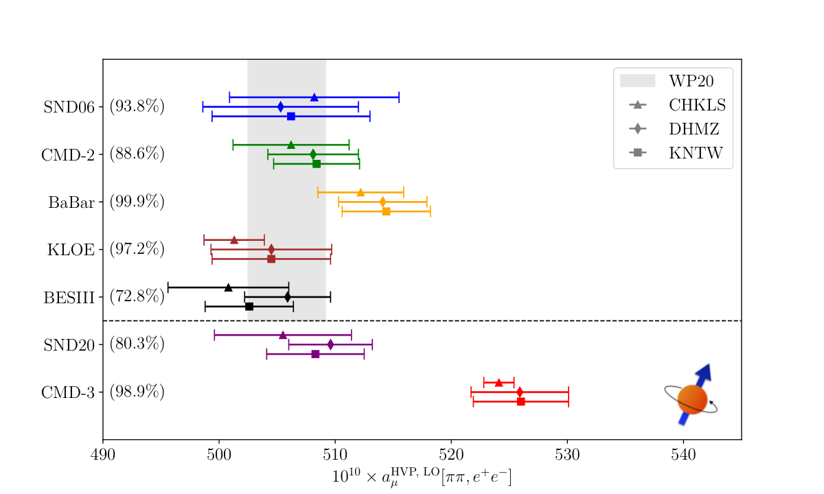
| Experiment | Percentage covered | |||
|---|---|---|---|---|
| CHKLS | DHMZ | KNTW | ||
| SND06 | ||||
| CMD-2 | ||||
| BaBar | ||||
| KLOE | ||||
| BESIII | ||||
| SND20 | ||||
| CMD-3 | ||||
| DHLMZ-23+LMR-24+WP25 | ||||
| Belle+CLEO+ALEPH+OPAL | ||||
Figure 26 presents a summary of the dispersive theoretical predictions for , based on various measurements of , treated using either of the “CHKLS” (Sec. 2.6.1), “DHMZ” (Sec. 2.5.1), and “KNTW” (Sec. 2.5.2) approaches. The various measurements cover the range from threshold up to according to the percentages indicated in the figure.
Contributions from other channels and from the high mass region above 1.8 GeV are based on WP20. It is, however, worth mentioning that significant progress has been made in these other channels since WP20 (see Sec. 2.2), e.g., next by uncertainty amplitude, the contribution from the process was improved by more than a factor of two. However, tensions between the Belle II data and previous measurements are now visible. Other discrepancies are observed in a few other channels as well—see the corresponding discussion in Sec. 2.3.6 in the context of Eq. 2.23—although their overall impact remains minor compared to the tension seen in the channel. Continued progress in the overall measurement program is essential for a future complete data-driven evaluation of .
The most important feature of Fig. 26 concerns the strong tensions observed among the available measurements, regardless of the various methodologies employed for the data integration and extrapolation/completion to the full mass range. The differences among the various methodologies are nevertheless also visible for the resulting central values and uncertainties, the latter differing up to a factor of two in some cases. This comes from different treatment of correlations for fits/weight derivation, strategies to complete the data sets, and usage of additional constraints. The increasing precision of data and the larger tensions among experiments highlight the importance of a conservative treatment of experimental systematic uncertainties. The conventionally used practice to treat the provided experimental systematic errors, whose knowledge is inherently limited, is generally incomplete compared to what was assumed by the measured data as discussed in Secs. 2.3.1–2.3.6 of WP20 and Secs. 2.2.1 and 2.6.1 of WP25. In some cases, this leads to an underestimation of the evaluated integral errors due to assumptions made for the correlations of systematic uncertainties or the energy-dependent amplitude of uncertainties.
The “CHKLS” Colangelo et al. [2019], Colangelo et al. [2022c], Stoffer et al. [2023], Leplumey and Stoffer [2025] points are obtained using a dispersive representation to implement constraints from analyticity, unitarity, and crossing symmetry, so that the cross sections can be analyzed in a global fit (with input for covariance matrices as provided by experiment), and thus the entire low-energy contribution can be evaluated for each experiment individually. In the figure, the variant of the dispersive approach without imposing the absence of zeros in the form factor is shown, see Sec. 2.6.1 for details, evaluated up to , with the remainder taken from WP20.
“DHMZ” perform a direct integration in the full range where a given measurement is available, complemented with data combinations for the rest, while “KNTW” limit their use of individual data to the upper range of 1 GeV, using data combinations for the remaining values. It is important to note that the latter combination-based integrals are by construction more precise than the integrals derived from one measurement alone (i.e., a measurement covering the low- and/or high-mass range can be misleadingly “penalized” when comparing the uncertainties). A local -based uncertainty rescaling is performed when necessary, although there are relatively little tensions in the relevant mass regions.
The “KNTW” numbers are solely based on the KNT19 combination Keshavarzi et al. [2018], Keshavarzi et al. [2020a] and are, in particular, deliberately not including the CMD-3 data (see Sec. 2.5.2 for further details). The combination is fully model-independent, incorporates experimental correlation information in data fits for the full available energy range whilst simultaneously avoiding procedural systematic biases (such as the d’Agostini bias in correlated fits D’Agostini [1994], Blobel [2003]), and determines additional systematic uncertainties.
The “DHMZ” result employs a spline-based relatively-local averaging (minimization of with correlations), with weight derivation accounting for different point-spacing/binning (see Sec. 2.5.1 for further details). All existing data are used on the full mass ranges where combinations are employed. The combination procedure is also validated through a closure test.
The “DHMZ” and “KNTW” direct integration methods yield similar values in most cases (differences not exceeding much more than 1 unit), except for the BESIII integral, where some difference (of about 3 units) arises due to the larger range on which the combined data are employed and the differences of methodologies discussed above and in WP20. The “CHLKS” points show lower uncertainties in a few cases, since the additional theoretical constraints in a global fit reduce the uncertainties in the resulting integral. This reduction is most effective in cases in which the data are relatively scarce in some energy region—the extreme case concerning the ability to extrapolate in a robust manner into regions in which no data were taken—and in which the systematic uncertainties, most prominently from the truncation of the conformal expansion, are small. In the latter case, as for CMD-3, the limited knowledge of exact correlations of the systematic uncertainties in experiment becomes more critical, suggesting to somewhat enlarge the fit uncertainties, see Secs. 2.2.1 and 2.6.1.

2.12 Summary and outlook
The unsatisfactory situation regarding the knowledge of the cross section for the process , which is known to contribute more than 70% to the total HVP dispersion integral, presents a significant limitation to the data-driven evaluation of the HVP contribution and, consequently, to the SM prediction of the anomalous magnetic moment of the muon. This is illustrated in Fig. 27. Since WP20, the introduction of the new CMD-3 measurement, which has a systematic uncertainty of 0.7%, has changed the landscape of hadronic cross-section measurements. The CMD-3 result provides a significantly higher value for the HVP contribution compared to older evaluations. Previously, for WP20, an averaging procedure with inflated uncertainties was adopted to accommodate the two most precise measurements from KLOE and BaBar, which exhibited already some discrepancies. However, this approach is no longer appropriate given the current situation with the new CMD-3 data. Due to the significant spread of experimental results, with relative differences exceeding the claimed systematic uncertainties by substantial factors, it has been decided not to perform a new average for the two-pion channel and, consequently, the HVP contribution within WP25. Clarifying the current situation is of utmost importance, and the following developments from the recent past and the near future will be essential for achieving progress:
- •
The detailed understanding and control of radiative corrections in experimental analyses have become a focal point of research in recent years. The availability of high-precision event generators, along with a well-defined understanding of their uncertainties, is fundamentally important for the field of hadronic cross-section measurements, as well as for the QED normalization processes utilized by experiments. All ISR experiments (BaBar BESIII, KLOE) use the NLO Phokhara event generator, which simulates hadronic and muonic events with one high-energy ISR (or FSR) photon representing the LO configuration. The dependence on Phokhara, however, strongly depends on the event analysis. The BaBar collaboration has conducted a detailed study on the fraction of (N)NLO photons and identified significant limitations of Phokhara in simulating these higher-order corrections Lees et al. [2023b]. They also found that the BaBar measurement, due to its highly inclusive selection of (N)NNLO photons, remains unaffected. A subsequent publication by the DHMZ group Davier et al. [2024a] explored the potential impact of these shortcomings on existing ISR publications for the process . Fast simulation by the DHMZ group suggested that the KLOE and BESIII measurements may have significantly underestimated the uncertainties attributed to radiative corrections. This latter claim holds especially for scenario 1 of the two scenarios considered in Ref. Davier et al. [2024a]. Further analysis by BESIII indicated that the large effect predicted for the BESIII measurement did not account for specific corrections implemented in the BESIII analysis Denig [2024]. Moreover, both KLOE and BESIII demonstrated agreement at the 1% level for the mass spectra for various event generators, which differ in their simulation of higher-order corrections Denig [2024], Venanzoni [2024]. As a result of these studies, it was concluded that scenario 1 in Ref. Davier et al. [2024a] seems unlikely, and the shortcomings of Phokhara most likely do not explain the seen differences between different measurements.
- •
The RadioMonteCarLow 2 initiative is committed to improving the theoretical predictions for hadron and lepton production at low-energy colliders by bringing the available MC generators to NNLO+ precision. In the first phase, a review of the existing state-of-the-art available generators has been concluded Aliberti et al. [2025]. The comparison was performed by using approximated experimental selections as benchmarks. The study will continue by incorporating additional important selection variables. Moreover, Ref. Aliberti et al. [2025] presents a detailed discussion of the different classes of higher-order radiative corrections for both direct-scan and ISR processes, identifying a critical class of virtual ISR corrections that, due to resonance enhancement, could contribute to the cross section at the relevant level (as first pointed out in Ref. Abbiendi et al. [2022]). A similar effect in the -odd asymmetry in direct-scan experiments was observed by CMD-3, demonstrating that such structure-dependent radiative corrections can indeed far exceed estimates in a form-factor-times-sQED prescription Ignatov and Lee [2022], Colangelo et al. [2022b]. Actual improvements to the codes are expected to take place during the next Phase II. To ultimately investigate the accuracy of event generators, high-quality codes with different approaches in simulating the radiative corrections are needed for cross-checks (both for energy scan and ISR experiments). The ongoing extension of the BabaYaga@NLO, Phokhara, McMule, and additional codes are important steps in that context.
- •
Fortunately, new precision measurements of the process are being prepared with significant effort by several experimental collaborations. The CMD-3 and SND experiments will continue their campaigns to analyze the energy scans conducted at the VEPP-2000 collider, while the BaBar, BESIII, and KLOE experiments will produce updated results using the ISR technique. For this purpose, considerably larger data sets will be utilized, and the event analyses will be designed to address possible limitations arising from event generators. In the case of BaBar a new analysis strategy based on angular fits will be employed. The Belle-II collaboration has already presented a preliminary precision ISR analysis for the channel Adachi et al. [2024] and will soon contribute to the leading two-pion channel as well.
- •
Theory developments since WP20 include the derivation and improvement of unitarity and analyticity constraints for the , , , and channels, with applications to chiral extrapolations, the determination of IB contributions, and structure-dependent radiative corrections. In addition, methods were developed to extract quark-flavor-specific results from the data. These efforts provide consistency checks on the data sets, establish correlations with other (low-energy) observables, and facilitate detailed comparisons to lattice-QCD calculations of HVP. Examples include the observed tensions with the dispersive constraints in the case of SND20 ()—while all other measurements pass the consistency check—and Belle II (); spread in the phase of the – mixing parameter and the charge radius among the experiments; predictions for IB in the long-distance tail of the QED correction due to the pion mass difference (as well as other IB effects); the derivation of theoretically robust amplitudes for structure-dependent radiative corrections; and the determination of data-driven comparison values for light-quark-connected and strange + disconnected Euclidean windows.
- •
The phenomenological analysis groups have made significant progress since the release of WP20. The DHMZ group has conducted detailed investigations to quantify the tensions among the various data sets, while the KNTW group has implemented the first fully blind data-driven HVP analysis and is in the process of scrutinizing, improving, and modernizing their data combination procedure. All these efforts over different groups are expected to lead to improved averaging procedures in the near future when the new data sets become available.
- •
The hadronic decay provides an alternative path to the dominant two-pion contribution to HVP. The data sets from the LEP experiments, CLEO, and Belle are consistent and provide a competitive uncertainty, with excellent prospects for further precision improvements with Belle-II measurements. The current uncertainty in the -based determination of HVP is dominated by challenging IB corrections. The two analyses by the DHLMZ and LMR groups have been combined to obtain the WP25 estimate: while the central value fully reflects the published results, the uncertainty has been reassessed to account for sources of IB that are not yet fully addressed in the literature. Work to tackle structure-dependent radiative corrections and IB effects in the ratio of EM and weak form factors is ongoing and new information is expected in the near future from dispersive methods, lattice-QCD, and data-driven constraints.
As an outlook, it can be stated that the coming years will bring a series of new experimental results for the dominant hadronic channels used to evaluate the HVP contribution to the anomalous magnetic moment of the muon. Both the BESIII and BaBar collaborations anticipate presenting new results for the dominant channel already in 2025. The increased sensitivity to the treatment of higher-order radiative corrections in the experimental analyses, along with the development of new event generators to support these analyses, marks a significant improvement and is expected to help clarify the current situation. Furthermore, upcoming new measurements of hadronic decays with unprecedented statistics will be performed at Belle II and will also be crucial to further improve the precision of the SM prediction of . In the more distant future, the MUonE experiment aims to provide an independent and inclusive approach to determining the HVP contribution by measuring the spacelike running of HVP. Additionally, new analyses and highly complementary analysis techniques will be developed, such as BESIII’s attempt to measure the inclusive hadronic cross section at low energies via ISR.
3 Lattice-QCD calculations of HVP
T. Blum, M. Bruno, M. Cè, D. Clarke, M. Della Morte, C. DeTar, A. X. El-Khadra, R. Frezzotti, G. Gagliardi, A. Gérardin, D. Giusti, S. Gottlieb, V. Gülpers, S. Kuberski, S. Lahert, C. Lehner, L. Lellouch, M. K. Marinković, H. Meyer, E. Neil, J. Parrino, A. Portelli, J. Sitison, J. T. Tsang, R. Van de Water, G. Wang, H. Wittig
3.1 Introduction
This section reviews lattice calculations of the HVP contributions to the muon . We start with an introduction summarizing standard definitions and the outcome of WP20. We adopt a Euclidean metric, which is the appropriate setup for lattice formulations. The position-space HVP tensor is given by the QCD and QED expectation value
| (3.1) |
where is the quark EM current
| (3.2) |
where, for a flavor , is the quark field and is the electric charge in units of the elementary charge. The current above is conserved in continuous space–time, and its implementation on a discrete space–time might differ in lattice-QCD calculations. The momentum-space HVP tensor is then given by the Fourier transform
| (3.3) |
The tensor above is known to be transverse as a consequence of gauge invariance and Ward–Takahashi identities, and can be described through a single form factor :
| (3.4) |
The function is known to be UV divergent, and is conventionally regularized by using the subtracted function , which fixes the residue of the photon propagator to one. Finally, with the definitions above, the LO HVP contribution to the muon is given by
| (3.5) |
where the kernel function is defined by
| (3.6) |
Equation 3.5 gives the spacelike analog of the timelike master formula Eq. 2.1, see also Sec. 4.1. In practice, it has become more standard in lattice calculations to evaluate the integral above on the time variable, for zero spatial momentum, as summarized below in Sec. 3.3. Furthermore, we define the LO HVP contribution, denoted by in Eq. 3.5, in terms of the current–current correlator restricted to one-photon-irreducible contributions.
We conclude this introduction by reviewing the status of lattice-QCD calculations of the LO HVP contribution to the anomalous magnetic moment of the muon at the time of WP20. Further details can be found in WP20 and references therein. Additionally, the definitions of the various components of are summarized in the next section. In WP20, six groups quoted complete results for the total LO HVP and were included in a world lattice average. Notice, however, that the disconnected contribution was computed on the lattice by only three groups, and some groups used phenomenological inputs in order to estimate the strong and QED isospin-breaking (IB) contributions. There was a relatively large spread among lattice results, but all calculations were in agreement, at the level. The final estimate was
| (3.7) |
with an uncertainty of 2.6%. As a consequence, the lattice world average was consistent with both the dispersive data-driven estimate and the “no new physics” scenario. The uncertainty was a factor of 4.5 larger than that of the data-driven estimate, and the lattice average was not included in the final SM value for . We also note that the BMW-20 Borsányi et al. [2021] lattice calculation, which reported a precision of 0.8%, was posted on arXiv after the WP20 deadline and published in April 2021. Consequently, it was not included in the WP20 lattice world average of Eq. 3.7.
Since none of the results retained in WP20 for the lattice HVP average of Eq. 3.7 included complete nonperturbative calculations of all components, it was decided to perform averages on individual contributions. In a second step, the errors of the individual contributions were added conservatively, assuming 100% correlation on the uncertainties, leading to the final result given by Eq. 3.7. The total uncertainty was dominated by the isospin-symmetric connected light-quark contribution, followed by strong IB (SIB) and QED corrections and the quark disconnected contribution. For the dominant light-quark contribution itself, the total error was dominated by the uncertainties associated with finite-volume (FV) corrections, statistics, and the continuum extrapolation. The uncertainties on the charm and strange quark contributions were already at or below the permil level relative to .
In order to achieve the permil-level precision needed to match the final Fermilab precision, the community identified a number of challenges early on. Within this section, we present in detail the progress made on them since WP20. Briefly, the main challenges and the progress made to address them so far are:
- •
FV corrections are significant, even on lattices, and are among the largest contributions to the total error quoted in Eq. 3.7. They can be estimated using EFTs or EFT-inspired models, including NNLO ChPT Bijnens and Relefors [2017], Aubin et al. [2016], Aubin et al. [2020a], Aubin et al. [2020b], the Chiral Model Chakraborty et al. [2017], the Meyer–Lellouch–Lüscher (MLL) formalism with a Gounaris–Sakurai parameterization of the timelike pion form factor (MLLGS) Meyer [2011], Francis et al. [2013], Della Morte et al. [2017], Gounaris and Sakurai [1968], and the Hansen and Patella formalism Hansen and Patella [2019], Hansen and Patella [2020]. However, there are now several direct FV studies also at the physical point Borsányi et al. [2021], Blum et al. [2025a], Djukanovic et al. [2025] that guide these extrapolations and provide well-quantified control over the associated uncertainties.
- •
The lattice scale uncertainty is amplified in by close to a factor of two Della Morte et al. [2017], due to its dependence on the muon mass, and, hence must itself be determined with permil-level precision. This is part of the program of every lattice collaboration engaged in an effort to compute HVP at permil-level precision.
- •
A permil determination of requires the full inclusion of IB effects even for quark-disconnected contributions. In principle, these effects also enter the determination of the lattice spacing. In WP20 only partial calculations of these effects were available, while now results for almost all IB effects are available from several groups Blum et al. [2018], Giusti et al. [2019b], Borsányi et al. [2021], Djukanovic et al. [2025], Bazavov et al. [2025a], except for a small fraction associated with sea–sea and sea–valence QED corrections, for which only one calculation exists Borsányi et al. [2021]. The long-distance (LD) QED contributions, which amount to about 0.3% of the total HVP, are, however, still a challenge.
- •
Many of these systematics (e.g., cutoff effects) are discretization dependent, so it is imperative to have results from different lattice actions. The results presented in this review employ gauge field ensembles generated independently by several lattice groups with improved gauge actions and a variety of different fermion actions, including Wilson-Clover, twisted-mass Wilson, Domain Wall, HISQ, and stout-smeared staggered fermion actions.
The rest of this section is organized as follows: Section 3.2 details the standardized lattice breakdown of into the isospin-symmetric flavor components and IB corrections. Section 3.3 is devoted to the discussion of some special features in the analysis of lattice calculations of HVP that are common to all calculations (e.g., blinding). Section 3.4 describes the calculation of time windows, which allow sharper and more detailed comparisons between lattice QCD calculations. Section 3.5 discusses the isospin-symmetric flavor contributions to the full Euclidean-time integration region. In Sec. 3.6, the results from the different collaborations are combined in order to produce a final estimate. The rest of the section describes the IB correction to the data from decays and the hadronic contribution to the running of . Those are presented in Sec. 3.7. Finally, possible cross-checks resulting from the use of alternative approaches such as the covariant coordinate-space representation are introduced in Sec. 3.8.
3.2 Breakdown of the total HVP contribution to into its various contributions
IB corrections to due to the mass difference between up and down quarks, as well as EM effects, are expected to be an correction relative to the total . Therefore, it is desirable to write
| (3.8) |
where denotes the isospin-symmetric component and the first-order IB corrections, which are sufficient in the present context. However, the separation above is not prescription independent. Indeed, since all quarks interact strongly and electromagnetically, any experimental input used to renormalize QCD and QED will only define the sum of the two terms above. Defining the individual terms requires additional conditions which define what physics is kept constant while taking to zero. This issue was discussed in the most recent FLAG review (cf. Sec. 3 in Ref. Aoki et al. [2024]), where a prescription referred to as the Edinburgh Consensus was agreed upon after consultation with the community. This scheme is the recommended prescription for future calculations. However, most calculations in the present review were initiated before the Edinburgh Consensus was agreed upon, and we will use a slightly modified prescription. We define isospin-symmetric QCD (isoQCD) to be the theory where quark masses are tuned to reproduce the following complete set of inputs
| (3.9) |
where is the Wilson flow scale introduced in Ref. Borsányi et al. [2012]. We call this prescription the WP25 scheme. The only difference between the WP25 scheme and the Edinburgh Consensus is the use of to set the QCD scale instead of the pion decay constant. Recent results estimated that this change does not generate significant deviations within the current level of uncertainty (cf. comparison in Sec. 3.4.4), although the matching between the two prescriptions will require more scrutiny in the future. Additionally, the variables used in the prescription above can be changed to other hadronic inputs while keeping the scheme fixed, although this change will generate an additional matching uncertainty in actual numerical calculations. Another set of variables introduced originally by the BMW collaboration Borsányi et al. [2021] are the connected meson masses , where for a quark flavor , is the mass of the pseudoscalar meson considering only quark-connected contributions. These masses, although purely theoretical, are well-defined quantities that can be matched to the physical inputs above. The scheme employed in BMW-20 Borsányi et al. [2021] resulted in isoQCD defined by
| (3.10) |
where is the current world average of the mass experimental measurements [Navas et al., 2024]. It was shown in BMW/DMZ-24 Boccaletti et al. [2024] that Eq. 3.10 matches Eq. 3.9 up to uncertainties small enough to be discarded in the context of the present review. Because of this, Eq. 3.9, or Eq. 3.10 with discarded uncertainties, may be referred to in the literature as BMW-20 or BMW scheme. In summary, we consider that it is well motivated to average results produced with either prescription, and that propagation of matching uncertainties is unnecessary at the current level of precision.
Furthermore, it is convenient to decompose into quark-disconnected and single-flavor quark connected contributions:
| (3.11) |
For a quark flavor , in the equation above is obtained from Eq. 3.5 by considering only the quark-connected contribution for flavor in the current–current correlator , and is the sum for all flavors of the remaining quark-disconnected contributions. We now discuss standard methodologies to predict the quantities defined in this introduction from lattice simulations.
3.3 Methodology
Here, we briefly discuss some of the methodology that is common to the lattice-HVP calculations presented in more detail below.
- •
Time–momentum representation (TMR): The TMR has become the standard method for estimating the LO HVP contribution using lattice methods Bernecker and Meyer [2011]. In this approach, Eq. 3.5 is re-written
(3.12) with the zero-momentum time correlator
(3.13) and the kernel function
(3.14) In the equations above, and are defined in Sec. 3.1. The function can be expressed in terms of a modified Bessel function of the second kind and Meijer’s function Della Morte et al. [2017] as
(3.15) where . The nonperturbative input computed on the lattice is the time correlator . Other approaches, based on a direct evaluation of the HVP tensor, (see, for example, Ref. Aubin et al. [2012]), or on the method of time moments introduced in Ref. Chakraborty et al. [2014] have been superseded by the TMR.
- •
Error treatment in HVP calculations: Lattice-QCD calculations yield ab initio theoretical predictions that are systematically improvable. Since lattice QCD is a MC method, statistical analysis is a crucial part of producing physical results. In addition to statistical errors from the MC process, systematic errors can enter in a variety of forms, for example, through truncating the functional form that guides continuum limit extrapolations of lattice data obtained at finite sets of lattice spacings. While the details may vary from group to group, all lattice analyses described below include estimates of systematic errors based on studies of variations of the functional forms of the underlying EFT expansions, e.g., consideration of various functional forms for continuum extrapolation, that allow the assessment of systematic errors associated with the respective extrapolation (or interpolation). More detailed discussions of specific types of systematic errors, for which the dominant uncertainties may be different for different windows, will be provided in context below.
- •
Blinding: Most of the HVP results presented below, including (for example) all three calculations discussed for the dominant LD light-quark connected contribution Blum et al. [2025a], Djukanovic et al. [2025], Bazavov et al. [2025b], are based on blinded analyses. Blinding has been used widely in lattice QCD for many years, to prevent the introduction of bias in calculations of quantities whose values are known either from experiment or from previous calculations. To conduct a blind analysis, a small but unknown blinding factor is introduced into the analysis, modifying the final HVP result. Different lattice groups introduce the blinding in different places, but most commonly the blinding is applied as part of the analysis code, which has the advantage that different blinding factors can be easily applied for different windows. As the precision of lattice calculations improves, the importance of blinding will only increase, and we encourage all groups to adopt blind analyses going forward.
- •
Treatment of correlations using FLAG procedure: Except where explicitly noted otherwise, to combine results from different lattice calculations, we adopt the procedure used by the FLAG group for averaging Aoki et al. [2024]. Central values in this procedure amount to uncorrelated weighted averages of individual central values, with statistical and systematic errors added in quadrature. Error bars for averages are constructed using a procedure by which 100% correlation can be assumed between specific contributions to individual error estimates, as described in Eqs. (7)–(10) of the reference. In cases where the overall per degree of freedom implied by the average over individual results is poor (i.e., ), a rescaling to increase the error bars by is performed to compensate.
In some cases, results for certain quantities from lattice groups have been superseded by updated calculations. Such superseded results are shown in tables and figures below, but are excluded from averages. Depending on the quantity considered, different sources of uncertainty are taken to conservatively be 100% correlated. This may include statistical uncertainties in cases where the two calculations share the same gauge configurations, or systematic uncertainties for shared FV correction schemes, valence quark discretization, or other sources of error as described below.
3.4 Window contributions
Dividing the Euclidean time integral into different ranges has proved to be a very valuable tool in comparing the results of various collaborations and also for comparison with calculations of HVP based on dispersion relations (where time ranges correspond to energy ranges). After defining the three windows most commonly used, we consider details of the results for each window.
3.4.1 Definitions
Breaking the time integral Eq. 3.12 into three components allows for a better separation of the different sources of uncertainty Blum et al. [2018]. The window contributions are defined by
| (3.16) | ||||
| (3.17) | ||||
| (3.18) | ||||
| (3.19) |
where
| (3.20) |
defines the window as a smooth function in Euclidean time. The width parameter , in particular, smooths out the window on both sides of the interval. The community advocated the use of the widely studied choice fm, fm, and fm Blum et al. [2018] as benchmark parameters. Each window can then be treated independently and extrapolated to the continuum and infinite-volume limits. With this choice, the intermediate window (W) is less sensitive to discretization effects than the short-distance (SD) window . It is also designed to be less sensitive to LD effects than the long-distance window and hence much less affected by the signal-to-noise problems at large .
3.4.2 Short-distance window
We begin by reviewing the SD window observable, denoted as and defined in Eq. 3.17. As in the case of the total LO HVP correction, also in the SD window region the most important hadronic contribution is the one due to the light - and -quark-connected contractions, , representing of , while the strange- and charm-quark-connected terms, and , constitute and of the total SD contribution, respectively. In Table 6 and Fig. 28, we collect results for the flavor-specific contributions, namely, , , and , as well as for the subleading correction reported by the various lattice QCD groups.
| Collaboration | |||||
|---|---|---|---|---|---|
| ETM-24 Alexandrou et al. [2025] | 2+1+1 | – | – | ||
| FNAL/HPQCD/MILC-24 Bazavov et al. [2025a] | 2+1+1 | ||||
| BMW/DMZ-24 Boccaletti et al. [2024] | 2+1+1 | ||||
| RBC/UKQCD-23 Blum et al. [2023] | 2+1(+1) | – | – | – | |
| ETM-22 Alexandrou et al. [2023a] | 2+1+1 | ||||
| QCD-22 Wang et al. [2023a] | 2+1(+1) | – | – | ||
| ETM-21 Giusti and Simula [2022] | 2+1+1 | – | – | – | |
| SL-24 Spiegel and Lehner [2025] | 2+1/0 | – | – | – | |
| Mainz/CLS-24 Kuberski et al. [2024] | 2+1 |
The calculations in BMW/DMZ-24 Boccaletti et al. [2024], Fermilab/HPQCD/MILC-24 Bazavov et al. [2025a], and ETM-22/24 Alexandrou et al. [2023a], Alexandrou et al. [2025] were performed on ensembles. Those in Mainz/CLS-24 Kuberski et al. [2024] and SL-24 Spiegel and Lehner [2025] are based on ensembles. The former allow SD matching to the full SM at renormalization scales equal to , up to corrections, while that scale is and corrections are of order for calculations based on ensembles. The Mainz/CLS-24 Kuberski et al. [2024] determination of , however, includes the leading correction due to the quenching of sea-charm quarks, estimating it to be at the level of based on perturbation theory Hoang et al. [1994]. The RBC/UKQCD calculation (RBC/UKQCD-23 Blum et al. [2023]) addresses that subleading systematic effect from first principles, by generating gauge ensembles with dynamical charm quarks matched to those with sea quarks, and finds it to be small compared to the quoted uncertainties. The gauge- and fermion-action dependence of the SD window is studied by the QCD group (QCD-22 Wang et al. [2023a]) using the overlap valence fermion action on ensembles with either the domain-wall fermion (and the Iwasaki gauge action) -flavor sea from the RBC/UKQCD collaboration or the highly-improved-staggered-quark (with the Symanzik gauge action) -flavor sea from the MILC collaboration. Further details of the lattice formulations adopted for the QCD action by the various groups can be found in the corresponding references indicated in Table 6.
The SD window observable can be obtained very precisely in lattice-QCD calculations as far as statistical errors are concerned, not being affected by the signal-to-noise problems present at large Euclidean time distances. FV effects, which typically represent a source of uncertainty relevant for the calculation of , play hardly any role in . Quantitatively, direct lattice evaluations, estimates based on ChPT and data-driven determinations point to sub-permil FV corrections for and physical Boccaletti et al. [2024]. As observed in Refs. Blum et al. [2023], Kuberski et al. [2024], Bazavov et al. [2025a] the dependence of on quark masses is mild as well. Also, the sensitivity to the lattice scale is found to be subdominant Alexandrou et al. [2023a], Kuberski et al. [2024]. On the contrary, the SD window suffers from large discretization effects, associated to the behavior of the lattice vector correlator at small-time distances, which are expected to be logarithmically enhanced with respect to the naive scaling typical of -improved calculations (compared to the usual case with on-shell observables), as discussed in Refs. Della Morte et al. [2009], Cè et al. [2021], Sommer et al. [2023], Alexandrou et al. [2023a]. Even though this may present a significant challenge, the comparison among the results obtained with different lattice regularizations provides the opportunity to test the robustness of the continuum-limit extrapolation.
The QCD action and the vector correlator employed in the calculations listed in Table 6 are -improved and all groups use data with at least three lattice spacings (or two lattice spacings and two or more lattice regularizations of the observable of interest) to control the extrapolation to the continuum limit. Furthermore, different strategies are adopted to reduce the impact of () lattice artifacts from very short Euclidean distances: in Refs. Alexandrou et al. [2023a], Blum et al. [2023], Boccaletti et al. [2024], Kuberski et al. [2024], Alexandrou et al. [2025], tree-level perturbative cutoff effects on lattice correlators are subtracted from the nonperturbative data; the use of a suitably subtracted SD TMR kernel function together with perturbative computations at very high momenta has been devised by the Mainz group Kuberski et al. [2024]; SL scrutinize the continuum limit of the SD window using purely lattice QCD methods, without perturbative input, via a combination of a quenched () continuum extrapolation with a separate one of the dynamical sea-quark corrections Spiegel and Lehner [2025]; while the Fermilab/HPQCD/MILC collaboration adopts a highly-improved vector-current discretization Bazavov et al. [2025a]. In the case of the staggered formulations adopted in Refs. Boccaletti et al. [2024], Bazavov et al. [2025a], additional lattice artifacts that generate the taste splittings among the pions are heavily suppressed in the SD window region and found to be negligible at the level of precision reached. The quality of the extrapolations to the continuum limit is shown in Fig. 29 through the examples of the computations of by BMW/DMZ-24, who use the largest number (seven) of lattice spacings, and of by ETM-24, who quote the smallest relative uncertainty for that flavor-specific contribution ().

All results presented in Table 6 are extrapolated to the continuum and infinite-volume limits and interpolated or extrapolated to the physical point. The quoted errors in all lattice results include statistical and systematic uncertainties, where the latter estimates effects from scale setting, input parameters, continuum extrapolation (which represents the main source of uncertainty in the case of ), infinite-volume extrapolation, and chiral interpolations/extrapolations. Typically, these systematic errors are estimated by varying the chiral, continuum, or FV fit functions, including adding higher-order terms in the corresponding EFT expansions, or varying which lattice data are included, among other things. Overall, agreement is observed among the various (seven), currently available and more recent determinations of the -quark connected contribution, shown in the upper-left panel of Fig. 28, with the most pronounced differences occurring between the calculations in Mainz/CLS-24 Kuberski et al. [2024] and BMW/DMZ-24 Boccaletti et al. [2024] on the one hand and those in ETM-22 Alexandrou et al. [2023a] and Fermilab/HPQCD/MILC-24 Bazavov et al. [2025a] on the other, at most at the level of about . As far as the -quark connected contribution is concerned, except for a tension between the ETM-24 Alexandrou et al. [2025] and Fermilab/HPQCD/MILC-24 Bazavov et al. [2025a] determinations, the five most up-to-date results, listed in Table 6 and collected in the upper-right panel of Fig. 28, exhibit good compatibility. The four results for and for (lower-left and -right panels of Fig. 28, respectively) from Refs. Alexandrou et al. [2023a], Boccaletti et al. [2024], Kuberski et al. [2024], Bazavov et al. [2025a], Alexandrou et al. [2025] are nicely consistent. For the -quark connected contribution the ETM, Mainz, and Fermilab/HPQCD/MILC groups provide the following estimates: Alexandrou et al. [2023a] (based on perturbation theory); Kuberski et al. [2024] (given by a combination of phenomenological/perturbative estimates Källén and Sabry [1955], Chetyrkin et al. [1996a], Chetyrkin et al. [1996b], Erler et al. [2021], and a nonrelativistic-QCD-based lattice calculation Colquhoun et al. [2015]); and Bazavov et al. [2025a] (from the direct lattice determination in Ref. Hatton et al. [2021] and pQCD inputs), respectively. Finally, the challenging nonperturbative calculation of the subleading IB contributions has been performed by only two collaborations so far. The Mainz group performs an explicit calculation of the IB corrections to the connected light- and strange-quark contributions due to unequal up- and down-quark masses (SIB) and electric charges de Divitiis et al. [2012], de Divitiis et al. [2013], while the QED correction to the charm-quark contribution is estimated in perturbation theory. IB effects in the lattice scale and in the quark sea, as well as quark-disconnected contributions in the calculation of the relevant correlation functions are neglected. The total quoted correction is Kuberski et al. [2024]. The Fermilab/HPQCD/MILC collaboration computes from first principles the LO SIB corrections for both the connected- and disconnected-quark contractions. QED corrections are estimated in perturbation theory. Higher-order contributions, including QED corrections to disconnected diagrams are neglected. The resulting SIB connected, SIB disconnected and Bazavov et al. [2025a] QED perturbative estimates yield a total SIB+QED contribution equal to .


To average the lattice results for , , , and given in Table 6, we use the strategy of the FLAG group described in Ref. Aoki et al. [2024]. Any result that has been updated or superseded by a more recent determination by the same lattice group is excluded from the average. In Table 6 superseded results are marked with an asterisk. In addition, the results from BMW/DMZ-24 are not yet published, hence are also excluded from the following average. We treat the statistical and systematic errors in QCD-22 Wang et al. [2023a] and RBC/UKQCD-23 Blum et al. [2023], QCD-22 Wang et al. [2023a] and Fermilab/HPQCD/MILC-24 Bazavov et al. [2025a], as well as in RBC/UKQCD-23 Blum et al. [2023] and SL-24 Spiegel and Lehner [2025] as 100% correlated since these calculations are based on overlapping MILC and/or RBC/UKQCD gauge configurations, (partially) on the same formulation of the QCD action, on common ensembles for the evaluation of systematic errors (such as FV corrections) and/or on common scale uncertainty. All the other determinations are treated as uncorrelated. Since sea-charm-quark effects on are found to be below the permil level (see the above estimate in QCD perturbation theory Kuberski et al. [2024]), we can combine and results in Table 6. Note that -quark effects are even more subleading and, therefore, can be neglected here. For the valence-bottom-quark-connected contribution, , we consider the uncertainties of the estimates mentioned above as 100% correlated, since the methods used by different teams to get them are similar. We provide an estimate for the SIB+QED IB corrections, , by combining the two previously described results given in Mainz/CLS-24 Kuberski et al. [2024] and Fermilab/HPQCD/MILC-24 Bazavov et al. [2025a] (see Fig. 30). Since both determinations come from first-generation calculations of some of those effects, we choose the conservative approach of averaging Mainz/CLS-24 and Fermilab/HPQCD/MILC-24 under the assumption that the uncertainties of the two calculations are 100% correlated. IB effects in the lattice scale and in the quark sea, as well as quark-disconnected QED contributions neglected in those calculations are expected to be small and, thus, covered by the quoted conservative error. The averages carry a in all cases.

Our averages for the individual flavor contributions to , in the isospin limit and for the leading SIB and QED corrections, are summarized in Table 7.
It should be stressed that the separation into isospin-symmetric flavor terms ( and ) and IB corrections is scheme dependent, while the sum of those contributions is unambiguous. We refer the reader to the various references given in Table 6 for details on the schemes adopted by the lattice groups. Here it is sufficient to note that ambiguities related to the different prescriptions used to define isoQCD with respect to the full QCD+QED theory are negligible for the SD window at the current permil precision level, as can be inferred from the very modest impact of variations in the lattice-scale setting Alexandrou et al. [2023a], Bazavov et al. [2025b] and quark-mass tuning Blum et al. [2023], Kuberski et al. [2024], Bazavov et al. [2025a] on .
The contributions in Table 7 can now be combined to obtain average lattice numbers for the SD window contribution to LO HVP in the isospin limit, . Adding to this result the SIB and QED corrections yields the LO HVP correction , which can be compared with the phenomenological determinations of (see also Figs. 38 and 39 below). A final choice has to be made on how to combine uncertainties in adding up the individual flavor and SIB+QED contributions. The uncertainty associated with the determination of the overall scale is 100% correlated among these contributions in a same calculation. Also, in a calculation of the various contributions performed on the same set of ensembles, statistical errors will be correlated. Thus, we choose the conservative approach of adding the errors of the individual contributions linearly in our final results. This procedure leads the following world average for the isospin-symmetric SD window contribution to the total LO HVP correction:
| (3.21) |
Adding to this result the average SIB+QED correction, we obtain the following lattice world average for the total SD, LO HVP contribution to the muon :
| (3.22) |
where we include subleading digits at intermediate stages before rounding to the digits shown. This result, which is roughly 10% of the total LO HVP contribution, has a relative uncertainty of about 0.4%, and it is compatible with the estimate from -ratio data given in Ref. Colangelo et al. [2022e] in the pre-CMD-3 scenario. The absence of significant tensions in comparing lattice and -data-driven results for is consistent with what is found for the HVP at large Euclidean momentum , as well as with the constraints from EW precision tests of the SM.
Another way of getting an average value for , though with a less conservative error, is to use directly the results quoted by a few groups, specifically by the ETM collaboration Alexandrou et al. [2023a], Alexandrou et al. [2025], by Mainz Kuberski et al. [2024], by Fermilab/HPQCD/MILC Bazavov et al. [2025a]. The average à la FLAG of those independent determinations, treating the errors as uncorrelated across calculations, amounts to which, remarkably, is in excellent agreement with our final value given in Eq. 3.22.
3.4.3 Intermediate window
The standard intermediate window observable contributing to the LO HVP term of is defined in Sec. 3.4.1, Eq. 3.18. Over the past few years the intermediate window has played an important role, since it allows for a high-precision comparison between SM predictions and experimental data for the annihilation cross section into hadrons in the CM energy range around . Indeed, from the perspective of lattice QCD, the computation of the intermediate window is significantly less challenging than that of the full HVP contribution. The LD tail of the vector correlator is exponentially suppressed by the integration kernel of , thereby mitigating both the signal-to-noise ratio issues that affect the correlator at large times and the large finite-size effects associated with two-pion states. Moreover, unlike the SD window, does not suffer from large cutoff effects. Altogether these features enable very precise lattice calculations of .
We first review results for that are given in isoQCD. Since tiny differences in the scheme defining isoQCD are present in the results obtained by the various groups we adopt the WP25 scheme as a reference scheme prior to building averages (see details below). Then we consider determinations of in QCD+QED as quoted by individual groups or coming from our average in the WP25-scheme isoQCD and from available estimates of IB effects (see Table 9).
We begin by separately discussing the connected light, strange, and charm quark contributions to in isospin-symmetric lattice QCD, denoted as , , and , respectively. For the connected -quark term, , which is by far the numerically dominant contribution to , we consider here all the lattice results obtained using data with at least one ensemble at the physical pion mass point, three lattice spacings (or two lattice spacings and two or more lattice regularizations of the observable), and . This criterion is relaxed for the subdominant contributions, where results based on two lattice spacings are also included. Since the deadline for inclusion in WP20, several lattice results have appeared: LM-20 Lehner and Meyer [2020], BMW-20 Borsányi et al. [2021], ABGP-22 Aubin et al. [2022], Mainz/CLS-22 Cè et al. [2022a], QCD-22 Wang et al. [2023a], ETM-22 Alexandrou et al. [2023a], RBC/UKQCD-23 Blum et al. [2023], Fermilab/HPQCD/MILC-23 Bazavov et al. [2023], BMW/DMZ-24 Boccaletti et al. [2024], and Fermilab/HPQCD/MILC-24 Bazavov et al. [2025a]. Concerning the lattice formulation adopted, LM-20, ABGP-22, Fermilab/HPQCD/MILC-23, and Fermilab/HPQCD/MILC-24 employ the HISQ staggered fermion discretization, BMW/DMZ-24 (BMW-20) use a staggered quark action with stout smearing (4stout), RBC/UKQCD use domain-wall fermions, ETM-22 use Wilson-Clover twisted-mass fermions, QCD-22 use overlap valence fermions on both domain-wall and HISQ sea, and Mainz/CLS-22 use -improved Wilson fermions. These determinations of the light-connected term, are collected in Table 8, and graphically shown in the upper-left panel of Fig. 31. Within the quoted (statistical plus systematic) errors a striking agreement is observed among all of them. The somewhat older and since superseded result from RBC/UKQCD-18 Blum et al. [2018] is also included in the table for completeness.
For the - and -quark connected contributions, and , new results have recently been presented by QCD-22 (-quark only), Mainz/CLS-22, ETM-22, BMW/DMZ-24, and Fermilab/HPQCD/MILC-24, with an additional update from the ETM collaboration (ETM-24 Alexandrou et al. [2025]). All currently available data for these contributions to the intermediate window are compiled in Table 8 and displayed in the upper-right and lower-left panels of Fig. 31. Overall, good agreement is observed among the various determinations of the -quark connected contribution, with the Mainz/CLS-22 result lying slightly above the other ones. For the -quark connected contribution, a somewhat larger spread is evident, with the most pronounced differences occurring between Fermilab/HPQCD/MILC-24 and RBC/UKQCD-18, and between Fermilab/HPQCD/MILC-24 and ETM-24, each at the level of about .
Turning to the quark-disconnected contribution to in isoQCD, which we denote as , six lattice results are available: RBC/UKQCD-18 Blum et al. [2018], BMW-20 Borsányi et al. [2021], Mainz/CLS-22 Cè et al. [2022a], ETM-22 Alexandrou et al. [2023a], BMW/DMZ-24 Boccaletti et al. [2024], and Fermilab/HPQCD/MILC-24 Bazavov et al. [2025a]. These are listed in Table 8 and shown in the lower-right panel of Fig. 31. The disconnected term gives only a tiny contribution to the total , of the order of , which is similar in size to the uncertainty on the dominant light-connected term. A moderate compatibility is observed overall among the different lattice results: the largest discrepancy, about , arises between the new BMW/DMZ-24 result and Mainz/CLS-22. We note that the BMW/DMZ-24 result is larger in magnitude than BMW-20 (which had a relative uncertainty of about ).
In order to average the lattice results for , we follow the procedure established by the FLAG group Aoki et al. [2024]. We exclude from the average any result that has been superseded by a more recent determination by the same collaboration, with the only exception of the BMW/DMZ-24 results, which have not yet been published. Consequently in our averages we use the BMW-20 determinations, supplementing them, when necessary, as specified in the caption of Table 8, with an additional systematic uncertainty. In Fig. 31, superseded results appear in gray, while in Table 8 they are indicated by an asterisk. The final central values are determined via an uncorrelated weighted average of the results, as described in Eqs. (3)–(6) of Ref. Aoki et al. [2024]. To estimate the final uncertainties, we apply the method summarized in Eqs. (7)–(10) of Ref. Aoki et al. [2024], which takes into account correlations among the various results. As a conservative choice, in averaging we assume a correlation in the statistical errors for groups that fully or partially share gauge configurations, and a correlation in the systematic errors for groups using the same discretization in the valence sector.
As anticipated, the average values for partial and total results in isoQCD are given in the reference WP25 scheme (see Sec. 3.2). Besides the BMW-20 and BMW/DMZ-24 results, the one of RBC/UKQCD-23 on , and the ones by Fermilab/HPQCD/MILC-24, the other intermediate-window results are given by the various authors in slightly different schemes: we do not alter their central values and errors in the tables and plots of this subsection, but in order to account for this systematic effect, prior to and only for the sake of averaging, we add in quadrature to the results not in the WP25 scheme a systematic uncertainty for , , , and a systematic uncertainty for . In almost all cases, this leads to a very small increase of the total errors and thus to a correspondingly slight decrease of the weight of these results in the average.
| FNAL/HPQCD/MILC-24 Bazavov et al. [2025a] | 2+1+1 | ||||
|---|---|---|---|---|---|
| ETM-24 Alexandrou et al. [2025] | 2+1+1 | – | – | ||
| BMW/DMZ-24 Boccaletti et al. [2024] | 2+1+1 | ||||
| FNAL/HPQCD/MILC-23 Bazavov et al. [2023] | 2+1+1 | – | – | – | |
| RBC/UKQCD-23 Blum et al. [2023] | 2+1 | – | – | – | |
| ETM-22 Alexandrou et al. [2023a] | 2+1+1 | ||||
| QCD-22 Wang et al. [2023a] | 2+1(+1) | – | – | ||
| Mainz/CLS-22 Cè et al. [2022a] | 2+1 | ||||
| ABGP-22 Aubin et al. [2022] | 2+1+1 | – | – | – | |
| BMW-20 Borsányi et al. [2021] | 2+1+1 | ||||
| LM-20 Lehner and Meyer [2020] | 2+1+1 | – | – | ||
| RBC/UKQCD-18 Blum et al. [2018] | 2+1 | ||||
| Average |
The value of the systematic uncertainty added in quadrature to the results not in the WP25 scheme can be justified as follows. Among the four renormalization inputs (for scale, -, -, -quark mass) that specify an isoQCD scheme, all lattice groups employ MeV to fix the -quark mass and MeV or a similar closely related input (e.g., ) to fix the -quark mass (which moreover has a tiny impact on the total ). One is thus only left with the ambiguities coming from use of different inputs as compared to the WP25 scheme about the scale and the -quark mass.
The scale input in the WP25 scheme, which originally in the BMW-20 results is given by fm (updated to fm by BMW/DMZ-24), is commonly replaced by MeV (used, e.g., by RBC/UKQCD-23 and Fermilab/HPQCD/MILC-24) or by the FLAG value of the pion decay constant MeV (used, e.g., by ETM-22/24, Mainz/CLS-22, and Fermilab/HPQCD/MILC-24). From RBC/UKQCD-23 we know that using the WP25 or the scale input leads to central value shift in . From the FLAG24 review Aoki et al. [2024] one learns that using as scale input leads to values of that are within 0.5% of the WP25 value. This can be seen in Table 77 of Ref. Aoki et al. [2024] by comparing the results for from ETM-21 Alexandrou et al. [2021], MILC-15 Bazavov et al. [2016], HPQCD13A Dowdall et al. [2013], and CLS-21 Strassberger et al. [2022] (the last one inferred by comparing the value of to that of ETM-21). Using the estimate (see, e.g., ETM-22, Eq. (A.20)) implies a systematic uncertainty on not larger than . Using analogous arguments and information on the spectral density of the current–current correlator in each flavor channel, a similar relative uncertainty due to the -scale ambiguity is estimated or expected for and , and a substantially smaller one for .

The systematic error we add to non-WP25 scheme results for is 0.3% because it amounts to the sum in quadrature of 0.2% arising from the scale ambiguity and another 0.2% due to the difference in -quark mass input for isoQCD as compared to the WP25 one. Indeed, from an unpublished analysis of ETM-24 data at four lattice spacings and physical pion mass we infer that the WP25 scheme input, which is the fictitious strange-strange quark-connected meson mass MeV, leads to a value of the kaon mass which is 0.7 MeV larger than MeV (used, e.g., by several lattice groups) and only 0.4 MeV smaller than MeV. Combining the fact that the input spread compared to WP25 is about 0.2% with the estimate of , which is provided by Mainz/CLS-22 (see Eq. (B.26) of Ref. Cè et al. [2022a]) and fully confirmed by ETM-24 unpublished data, we estimate a systematic uncertainty of less than 0.2% on due to ambiguity in the -quark input for isoQCD.
The averages of the single-flavor and disconnected contributions obtained in this way are provided in the last row of Table 8 and illustrated by the colored vertical bands in Fig. 31. In the case of , the reduced of the fit is approximately 3 and, due to the lower level of compatibility among the lattice results in this case, we inflate the final uncertainty by a factor of .*¶*¶ *¶ For , the reduced of the fit is slightly larger than one (about 1.3), too, and we inflated the final error by a factor .
We now turn to the results for in isoQCD. There are five groups who provided (or provided sufficient evidence to infer) results on : Fermilab/HPQCD/MILC, BMW, RBC/UKQCD, ETM, and Mainz. The results are summarized in Table 9 and shown in the left panel of Fig. 32. For BMW/DMZ-24, we sum the single-flavor and disconnected contributions, combining their errors in quadrature. Instead, ETM-22, Mainz/CLS-22, and Fermilab/HPQCD/MILC-24 directly quote the value of . For RBC/UKQCD-23/18, we begin with the value of quoted in the WP25 scheme Blum et al. [2023] and then add the - and -quark connected contributions, as well as the disconnected contribution given in Ref. Blum et al. [2018]. Because these three contributions are not originally provided in the WP25 isoQCD scheme, we assign systematic errors of , , and , respectively, before summation. The resulting RBC/UKQCD value and error are then treated as if given in the WP25 scheme. As for BMW-20, we subtract an IB correction from the total computed in QCD+QED.
| FNAL/HPQCD/MILC-24 Bazavov et al. [2025a] | 2+1+1 | |||
|---|---|---|---|---|
| BMW/DMZ-24 Boccaletti et al. [2024] | 2+1+1 | Borsányi et al. [2021] | ||
| RBC/UKQCD-23/18 Blum et al. [2023], Blum et al. [2018] | 2+1 | |||
| ETM-22 Alexandrou et al. [2023a] | 2+1+1 | Borsányi et al. [2021] | ||
| Mainz/CLS-22 Cè et al. [2022a] | 2+1 | |||
| BMW-20 Borsányi et al. [2021] | 2+1+1 | |||
| Average |
In analogy to the procedure above, the average of results for is also given in the WP25 isoQCD scheme. In order to account for the slightly different definitions of the isoQCD entering the results by ETM and Mainz in Table 9, we add, prior to averaging, a systematic uncertainty of (i.e., the same systematic error we attributed previously on ) to all results not quoted in the WP25 isoQCD scheme. The average, performed according to the FLAG procedure just as for the partial single-flavor and disconnected contributions, yields*∥*∥ *∥ As in the case of the single-flavor and disconnected contributions, since the BMW/DMZ-24 results have not yet been published, we base our averages on the BMW-20 determinations (see also the caption of Table 9).
| (3.23) |
with an uncertainty of about 0.15%.
An alternative procedure to obtain is to sum the (average of) single-flavor and disconnected contributions listed in the last row of Table 8. Noting that the quark-connected correlators for different flavors and the quark-disconnected correlators all have very different statistical fluctuations, reflecting the completely different physics of the corresponding intermediate-state channels, we expect their statistical correlations to be tiny already within the results of a single group and further diluted by the average leading to last line of Table 8, and hence safely negligible. For this reason we proceed by adding the uncertainty of these contributions in quadrature to obtain
| (3.24) |
This result is in excellent agreement with that of Eq. 3.23. If one were to treat the individual flavor contributions as fully correlated one would obtain a result with a 36% larger uncertainty, namely
| (3.25) |
For the reasons outlined above, we consider this latter value to be overly conservative and advocate the value given in Eq. 3.24 as our central result for the isospin-symmetric window contribution in the WP25 scheme.
To provide a QCD+QED result with a conservative error for we add the average of IB effects to the result Eq. 3.24 obtaining the value
| (3.26) |
The estimates of the IB effect with respect to isoQCD in the WP25 scheme are given for each group in the last column of Table 9. For the cases where the value of is not taken from the BMW-20 paper, we proceed as follows: for Fermilab/HPQCD/MILC-24 and RBC/UKQCD-23/18 we obtain it by combining the published information on the correlated difference in between the used scheme and the WP25 scheme with the requirement that the sum be scheme independent; for Mainz/CLS-22 we keep the published central value of in the scheme of choice, assuming that the scheme dependence is accounted for in the estimated systematic error.
Another way of obtaining a final result for is to use directly the results quoted in QCD+QED by a few groups, see the corresponding column of Table 9. An average à la FLAG leads to , which is reassuringly in very good agreement with the value in Eq. 3.26.
Finally, we stress that the result of Eq. 3.26 is potentially of high relevance for the experimental collaborations measuring and for precision tests of the SM. Indeed, the quantity can be accessed experimentally and lattice QCD+QED provides for it a pure SM prediction with an accuracy of about 0.18%.

3.4.4 Long-distance window
A precise estimation of the LD contribution is crucial for achieving high precision in , as it dominates both the central value and the uncertainty in lattice-QCD calculations. The latter arises primarily from the exponential signal-to-noise problem, which results in larger statistical uncertainties compared to and . Additionally, significant FV effects pose challenges for conventionally sized lattices with at the physical value of the pion mass. Moreover, when the staggered fermion formulation is used to simulate quark fields, substantial taste-breaking effects introduce deviations from the continuum theory, further complicating the continuum extrapolation.
Four groups have performed dedicated computations of contributions to the LD window . RBC/UKQCD-24 Blum et al. [2025a], Mainz/CLS-24 Djukanovic et al. [2025], and Fermilab/HPQCD/MILC-24 Bazavov et al. [2025b] have all evaluated the dominant light-quark connected contribution to . In addition, Mainz/CLS-24 provide results for the remaining flavor contributions, yielding a complete determination of the LD window in isoQCD. The ETM collaboration has computed the subleading strange- and charm-connected contribution to in ETM-24 Alexandrou et al. [2025].
The RBC/UKQCD collaboration employs simulations with flavors of domain-wall fermions at three lattice spacings, down to . Three ensembles at physical quark masses are complemented by six simulations with heavier-than-physical pion masses. A spectral reconstruction of the vector correlation function from two-pion states is used to reduce statistical noise in the LD regime. The Mainz calculation is based on flavors of -improved Wilson fermions at six lattice spacings, with the finest reaching . The analysis includes 34 gauge ensembles with pion masses ranging from down to , including three ensembles with physical quark masses. Low-mode averaging is supplemented by a spectral reconstruction on selected ensembles to compute the vector correlation function. Fermilab/HPQCD/MILC use four ensembles with flavors of highly improved staggered quarks, all at physical quark masses. The finest ensemble corresponds to a lattice spacing of . Low-mode averaging is used for the vector correlation function, and EFT-based taste-breaking corrections are applied alongside finite-size corrections to mitigate cutoff effects specific to the staggered formulation. The ETM collaboration computes - and -quark connected correlation functions on six physical-mass ensembles with flavors of twisted-mass fermions at four lattice spacings, with the finest being .
Currently, no lattice calculation exists for IB effects in the pure LD regime, restricting the averaging of results to the isospin-symmetric case. Given the enhanced scale dependence of compared to and , and the fact that IB corrections primarily affect large Euclidean distances, a significant dependence on the scheme used for isoQCD cannot be excluded at present. To mitigate this and enable meaningful comparisons and averaging of lattice-QCD results, groups computing the light-connected contribution to have performed their analyses in multiple schemes.
RBC/UKQCD-24 quote results in the RBC/UKQCD-18 scheme Blum et al. [2018] as well as in the WP25 scheme, both of them using the baryon mass to set the scale. Mainz/CLS-24 provide results in a scheme defined in Ref. Cè et al. [2022a], which employs a combination of the pion and kaon decay constants, and , to set the scale, as well as in the WP25 scheme. Similarly, Fermilab/HPQCD/MILC-24 quote results in two schemes that differ only in the scale-setting quantity, either or , and also in the WP25 scheme. ETM-24 employ the scheme of the Edinburgh consensus based on to set the scale.
While the values provided by the collaborations in the WP25 scheme are expected to match within the quoted uncertainties, the degree to which the collaboration-specific - and -based schemes differ has not yet been systematically studied. We recognize that the spread of the -based schemes between Fermilab/HPQCD/MILC-24 and Mainz/CLS-24 is significant and needs to be scrutinized in future work. To account for this effect in WP25, we consider additional averages in the WP25 scheme with Fermilab/HPQCD/MILC-24 and Mainz/CLS-24 excluded, respectively. We then take half of the difference of the central value of those two averages as an additional uncertainty that is added in quadrature, following the approach adopted in WP20 for the BaBar–KLOE tension of the data-driven HVP evaluation. As a result, an average of the three results for the light-quark connected contribution can be robustly performed in the WP25 scheme. The results across all schemes are summarized in Table 10 and shown in Fig. 33 for the common WP25 scheme.
| WP25 | Own scheme () | Own scheme () | ||
|---|---|---|---|---|
| FNAL/HPQCD/MILC-24 Bazavov et al. [2025b] | 2+1+1 | |||
| Mainz/CLS-24 Djukanovic et al. [2025] | 2+1 | – | ||
| RBC/UKQCD-24 Blum et al. [2025a] | 2+1 | – |
While all three results are statistically independent, they adopt similar approaches to correct for finite-size effects. RBC/UKQCD-24 apply the method developed by Hansen and Patella Hansen and Patella [2019], Hansen and Patella [2020]. Mainz/CLS-24 employ the same method for short Euclidean distances, complemented at larger distances by the Meyer–Lellouch–Lüscher (MLL) formalism, which uses a Gounaris–Sakurai parameterization of the timelike pion form factor Meyer [2011], Francis et al. [2013], Gounaris and Sakurai [1968].****** *** A recent study finds that the MLL formalism is valid at all Euclidean distances and reproduces the result of Hansen–Patella by including sufficiently high-energy two-pion states Itatani et al. [2025]. Both studies explicitly validate these corrections through measurements in multiple volumes with identical Lagrangian parameters. Fermilab/HPQCD/MILC-24, on the other hand, perform a model average over three different approaches to account for FV effects, including the MLL method. RBC/UKQCD-24, Mainz/CLS-24, and Fermilab/HPQCD/MILC-24 estimate the uncertainty for the light-connected contribution arising from FV corrections to be 0.8, 1.7, and 1.4 units of , respectively. To ensure a conservative assessment, we adopt these values as a correlated contribution to the systematic uncertainty across all three results.

When averaging according to the FLAG procedure, we apply a slight rescaling of to account for the fact that the result from Fermilab/HPQCD/MILC-24 is significantly smaller than the other two. The -value of the average is . The outcome of the partly correlated average, combined with the additional systematic uncertainty of , is
| (3.27) |
where the contribution of the uncertainty of that is part of the scheme definition is not included. This uncertainty originates from the determination of the physical value of the gradient flow scale fm, based on in Ref. Borsányi et al. [2021]. The average is displayed as a blue band alongside the three inputs in Fig. 33.
To compute the full LD window observable, the averaged result for the isovector contribution can be combined with the Mainz/CLS-24 determination of the isoscalar contribution within the WP25 scheme. The strange-connected contribution is included in the isoscalar part. Its determination in Mainz/CLS-24 is slightly larger than, but statistically compatible with, the result from ETM-24, where the two employed schemes are similar but not identical. The charm-connected contribution, computed in Mainz/CLS-24 and ETM-24, is numerically negligible at the current level of precision and has not been obtained in the WP25 scheme in either work. We note that this procedure uses the LD disconnected and strange contributions from only Mainz/CLS-24.
By adding the averaged isovector contribution, , to the isoscalar contribution, Djukanovic et al. [2025], one obtains
| (3.28) |
for the LD window observable in isoQCD within the WP25 scheme, again without scale uncertainty.
3.5 Flavor decomposition
In this section, we summarize the results for flavor specific contributions to . Following the breakdown in Eq. 3.11, we consider the light-, strange-, and charm-quark connected contributions, followed by a discussion of the disconnected contribution. These results are obtained by considering the individual flavor contributions over the entire integration range. In principle, this corresponds to performing the integral of Eq. 3.12. However, in practice, the results are now more commonly obtained from summing the contributions to the three windows as in Eq. 3.16. This summed approach leverages the fact that each window contribution has a tailored analysis, resulting in a more robust determination, once inter-window correlations are taken into account Blum et al. [2025a], Djukanovic et al. [2025], Bazavov et al. [2025b]. Final averages are given in the WP25 isospin-symmetric scheme of Eq. 3.9. Where possible, results in figures are also presented in this scheme.
| FNAL/HPQCD/MILC-24 Bazavov et al. [2025b] | 2+1+1 | – | – | – | |
|---|---|---|---|---|---|
| ETM-24 Alexandrou et al. [2025] | 2+1+1 | – | 53.57(41)(48) | 14.56(10)(9) | – |
| Mainz/CLS-24 Djukanovic et al. [2025] | 2+1 | 675.7(4.1)(3.7) | 54.5(3)(3) | 14.4(2)(2) | |
| RBC/UKQCD-24 Blum et al. [2025a] | 2+1 | 668.7(6.1)(2.9) | – | – | – |
| ABGP-22 Aubin et al. [2022] | 2+1+1 | 646 (11.4)(7.8) | – | – | – |
| HPQCD-20 Hatton et al. [2020] | 2+1+1 | – | – | – | |
| LM-20 Lehner and Meyer [2020] | 2+1+1 | 657(26)(12) | 52.83(22)(65) | – | – |
| BMW-20 Borsányi et al. [2021] | 2+1+1 | 652.4(2.0)(5.3) | 53.393(89)(68) | 14.6(0)(1) | |
| ETM-18/19 Giusti et al. [2018], Giusti and Simula [2019] | 2+1+1 | 629.1(13.7) | 53.1(1.6)(2.0)∗ | 14.75(42)(37)∗ | – |
| Mainz/CLS-19 Gérardin et al. [2019a] | 2+1 | 674(12)(5)∗ | 54.5(2.4)(0.6)∗ | 14.66(45)(6)∗ | |
| ABGP-19 Aubin et al. [2020a] | 2+1+1 | 659(22)∗ | – | – | – |
| FNAL/HPQCD/MILC-19 DeTar et al. [2019] | 2+1+1 | 637.8(8.8)∗ | – | – | – |
| PACS-19 Shintani and Kuramashi [2019] | 2+1 | 673(9)(11) | 52.1(2)(5) | 11.7(0.2)(1.6) | – |
| RBC/UKQCD-18 Blum et al. [2018] | 2+1 | 649.7(14.2)(4.9)∗ | 53.2(4)(3) | 14.3(0)(7) | |
| BMW-17 Borsányi et al. [2018] | 2+1+1 | 647.6(7.5)(17.7)∗ | 53.73(4)(49)∗ | 14.74(4)(16)∗ | |
| HPQCD-14 Chakraborty et al. [2014] | 2+1(+1) | – | 53.41(0)(59) | 14.42(0)(39)∗ | – |
For the dominant light-quark connected component , which accounts for of the total HVP contribution, there have been six new results since the release of WP20: BMW-20 Borsányi et al. [2021], LM-20 Lehner and Meyer [2020], ABGP-22 Aubin et al. [2022], RBC/UKQCD-24 Blum et al. [2025a], Mainz/CLS-24 Djukanovic et al. [2025], and Fermilab/HPQCD/MILC-24 Bazavov et al. [2025b]. The first three are obtained from an analysis of the full integral, whereas the latter three come from summing the windows. These six new results are collected in the third column of Table 11, along with previous determinations that were included in WP20. All these new results (aside from LM-20) are updates on previous determinations, which we denote with an asterisk in the table. As discussed in Sec. 3.4.4, a central component of these newer calculations (aside from LM-20) is the use of exact low-modes of the Dirac operator, which is the primary reason for the dramatic improvement in statistical precision over older determinations. The four most precise determinations are all also available in the WP25 isospin-symmetric scheme, which we collect in Table 12.
For the strange and charm connected components, which are and of the total HVP contribution, respectively, there are four new determinations of , from BMW-20 Borsányi et al. [2021], LM-20 Lehner and Meyer [2020], Mainz/CLS-24 Djukanovic et al. [2025], and ETM-24 Alexandrou et al. [2025], and four new determinations of , from BMW-20 Borsányi et al. [2021], HPQCD-20 Lehner and Meyer [2020], Mainz/CLS-24 Djukanovic et al. [2025], and ETM-24 Alexandrou et al. [2025], since WP20. These are given in the fourth and fifth columns of Table 11. Again, aside from LM-20, these supersede previous determinations from the same groups. Finally, for the disconnected contribution , given in the last column of Table 11, there have been two new results, BMW-20 Borsányi et al. [2021] and Mainz/CLS-24 Djukanovic et al. [2025], both updates on previous determinations.
| FNAL/HPQCD/MILC-24 Bazavov et al. [2025b] | 2+1+1 | – | – | – | |
|---|---|---|---|---|---|
| Mainz/CLS-24 Djukanovic et al. [2025] | 2+1 | 666.2(4.9)(6.1) | 53.56(21)(33) | – | |
| RBC/UKQCD-24 Blum et al. [2025a] | 2+1 | 666.2(4.3)(2.5) | – | – | – |
| BMW-20 Borsányi et al. [2021] | 2+1+1 | 652.4(2.0)(5.3) | 53.393(89)(68) | 14.6(0)(1) |
The results for each contribution are compared in Fig. 34, where we show superseded results with a gray marker.*††*†† *†† The results of Refs. Chakraborty et al. [2017], Della Morte et al. [2017] are not included in the comparison, because they were already superseded in WP20 by newer results. We stress here, as in Sec. 3.4.4, that these determinations, in particular and , are sensitive to how one defines the isospin-symmetric pure QCD scheme. Hence, when comparing results directly one should be aware of the particular scheme definitions, which are described in the caption and references of Tables 11 and 12.
We perform the world averages for each of the flavor contributions using two independent approaches. The first approach makes direct use of the results in Tables 11 and 12. For this, we follow the FLAG averaging procedure discussed at the end of Sec. 3.3. In particular, results that have been superseded are not included, as well as results based on less than three lattice spacings for dominant contributions and less than two for subdominant ones. Before performing the averages, the results that are not in the preferred isospin-symmetric scheme of Eq. 3.9 must be adjusted. To do this we follow the strategy laid out in Sec. 3.4.3.
| Avg. A | |||||
|---|---|---|---|---|---|
| Avg. B |
For , the results from Fermilab/HPQCD/MILC-24 Bazavov et al. [2025b], RBC/UKQCD-24 Blum et al. [2025a], and BMW-20 Borsányi et al. [2021] are available in the preferred scheme, which relies on to determine in fm. The result from Mainz/CLS-24 Djukanovic et al. [2025] is not; however, the corresponding determination of is available in the WP25 scheme, which can be combined with the relatively scale-insensitive short- and intermediate-distance contributions. All these WP25 determinations are given in Table 12. The remaining results, ABGP-22 Aubin et al. [2022], LM-20 Lehner and Meyer [2020], ETM-18/19 Giusti et al. [2018], Giusti and Simula [2019], and PACS-19 Shintani and Kuramashi [2019], all have significantly larger uncertainties and use directly to set the scale or to determine in fm. Hence, for this average, we include only the four sub-percent results in the WP25 scheme. We account for correlations due to the shared approaches to correct for FV effects in the same fashion as in Sec. 3.4.4. In addition, we correlate the systematic uncertainty due to taste-breaking effects from BMW-20 and Fermilab/MILC/HPQCD-24, corresponding to 3.7 and 0.9 in units of , respectively. The additional uncertainty of from the spread of the -based LD window results in Sec. 3.4.4 is also applied to here.
For , there are only two*‡‡*‡‡ *‡‡ The Mainz/CLS-24 result in the WP25 scheme is constructed in the same fashion as described for the result, with an additional 0.3% relative uncertainty applied to the component. This additional 0.3% uncertainty is estimated in Sec. 3.4.3. results available in the WP25 scheme (see Table 12), hence, following Sec. 3.4.3, for results not in this scheme we include an additional 0.9% and 0.2% systematic uncertainty (in quadrature) due to scale setting input and the spread in input values for . These relative uncertainties are estimated using the derivatives and (Eq. (B.29) of Ref. Cè et al. [2022a]). As the charm contribution is dominated by and we assign just the systematic uncertainty obtained in Sec. 3.4.3.†*†* †* For results obtained using as opposed to as in Eq. 3.9, namely HPQCD-20, we include a 0.5% systematic uncertainty, estimated similarly as described for . Finally, for the disconnected contribution, there are only two qualifying results obtained from a lattice calculation with more than one lattice spacing, BMW-20 Borsányi et al. [2021] and Mainz/CLS-24 Djukanovic et al. [2025]. The BMW-20 result is already in the preferred scheme, whereas the Mainz/CLS-24 result can be obtained by the same procedure as described above for . This first set of flavor averages (Avg. A), as well as the corresponding result for , is collected in the first row of Table 13. We note here that the average is largely dominated by the BMW-20 result, with a weight of 0.84. This is due to it being one of only two results already in the WP25 scheme, and already having smaller errors than all other determinations.

The second approach for obtaining world averages is to make use of the windowed averages obtained in Secs. 3.4.2, 3.4.3, and 3.4.4. For the short- and intermediate-distance windows, the separate flavor averages are all performed in the WP25 scheme. For the LD window, the light-quark contribution of Eq. 3.27 is also obtained in the WP25 scheme. Due to the sensitivity of to the choice of scale-setting and strange-quark mass input, we take the sole determination in the WP25 scheme from Mainz/CLS-24 Djukanovic et al. [2025] as our window-‘‘average’’ for this quantity.†††† †† The other determination of this quantity from ETM-24 Alexandrou et al. [2025] uses to set the scale as opposed to via as in the WP25 scheme Eq. 3.9. The shift in from the two scale-setting choices can be estimated using the two results for in Ref. Djukanovic et al. [2025](Table 3 and Eq. (A.9)), giving . Including this shift as an additional source of uncertainty on the result of Ref. Alexandrou et al. [2025] dramatically inflates the overall error and renders a FLAG average of the two results pointless. The LD charm contribution, , is almost negligible since it contributes less than to the charm total. In addition, the sensitivity of to the choice of scale setting is suppressed by the large value of the ratio . To obtain , we perform a FLAG average of the two determinations of this quantity from Mainz/CLS-24 Djukanovic et al. [2025] and ETM-24 Alexandrou et al. [2025]. For the LD disconnected contribution , we take the only available determination of this quantity from Mainz/CLS-24 Djukanovic et al. [2025].
With all these results in hand, the sum in Eq. 3.16 can be performed for each flavor. Given the conservative choices made to account for correlations between groups in Secs. 3.4.2 and 3.4.3, we perform an uncorrelated sum of the windows to obtain the window-summed averaged values for and . For and , a systematic uncertainty that is common to all determinations of these quantities in the W and LD windows concerns the EFT-based approaches to correcting for FV effects. To account for this, we assume 100% correlation of FV uncertainty between the intermediate and LD windows. To obtain a correlation coefficient that corresponds to this assumption, we examine results from the three groups that have both and determinations Cè et al. [2022a], Blum et al. [2023], Blum et al. [2025a], Djukanovic et al. [2025], Bazavov et al. [2025a], Bazavov et al. [2025b]. In particular, we compute the following correlation coefficient , where is the uncertainty due to FV, for each case. A weighted average of is obtained using the weights from the FLAG average in Eq. 3.27. This value is used for as well. The final window-summed averaged results (Avg. B) are given in the second row of Table 13. We note here that the Avg. B determination of neglects the nontrivial anti-correlations between the Mainz/CLS-24 results for and , which arise when obtaining these flavor contributions from linear combinations of and as in Ref. Djukanovic et al. [2025]. Therefore, the uncertainty on this determination of is less well estimated than that of Eq. 3.29 discussed in Sec. 3.6.
We observe that all values from this second average are broadly consistent with the averages from the first approach. The central value of from Avg. A is slightly lower than Avg. B and its uncertainty is smaller. This is due to the LD contribution from BMW-20 playing a part in the first average but not in the second. For the same reason, the uncertainty in is significantly smaller in the first average.
Comparing the two averages further, we note that every flavor-specific average that enters Avg. A is based on three or more inputs, while Avg. B takes as inputs for and a result from a single lattice group. However, Avg. A excludes some of the most recent results for the and contributions, particularly for the and flavor contributions. We can consider a variation to Averages A and B, where (almost) all recent results are included and where all contributions are based on two or more inputs, by combining and from Avg. A with and from Avg. B. This yields the value , which is virtually identical to Avg. B and to the average in Eq. 3.29 in Sec. 3.6.1. Other variations yield similar results.
3.6 Total HVP
In this section, we present our averages for the total HVP contribution to computed in lattice QCD. When combined with QED, EW, and the remaining hadronic contributions (also computed using lattice methods), these averages yield purely theoretical SM predictions for . We emphasize that most of the values from individual groups that comprise our averages have used blinding procedures, and we use the FLAG averaging procedure throughout.
Since the pioneering works of Blum Blum [2003] and Aubin and Blum Aubin and Blum [2007], and the seminal paper of ETM in 2011 Feng et al. [2011] in two-flavor QCD, many lattice calculations of have been performed Burger et al. [2014], Chakraborty et al. [2017], Borsányi et al. [2018], Della Morte et al. [2017], Blum et al. [2018], Giusti et al. [2018], Giusti and Simula [2019], Gérardin et al. [2019a], Davies et al. [2020], Shintani and Kuramashi [2019], Borsányi et al. [2021], Boccaletti et al. [2024], Djukanovic et al. [2025], Blum et al. [2023], Blum et al. [2025a], Aubin et al. [2022]. In addition to these, there are now many works giving the individual windows and other contributions as discussed in the previous two sections Lehner and Meyer [2020], Wang et al. [2023a], Cè et al. [2022a], Alexandrou et al. [2023a], Kuberski et al. [2024], Spiegel and Lehner [2025], Alexandrou et al. [2025], Bazavov et al. [2025a], Bazavov et al. [2025b]. Hence, to obtain a final lattice prediction for , there are a number of ways to combine the lattice results from the various groups. These differ in the contributions to that are averaged before being combined. Since groups do not necessarily compute all contributions, it matters in which order they are averaged and added up. Here we consider four different combinations:
- 1.
Total from a combination of the averages of all available lattice results for the SD, W, and LD windows in the isospin-symmetric limit plus the average of the total IB corrections: The advantage of this approach is that there are many results for some flavor components of the isospin-symmetric windows (see Table 8). This is particularly true for the contribution to the intermediate-distance window for which there are eleven results and, more generally, for all flavor contributions to that window. While this large number of computations allows a particularly robust estimate of the corresponding systematic errors, this intermediate-distance window contributes only about 35% to the total. There is also a fair number of computations of the SD window (see Table 6). For the LD window, which contributes 55%, the situation is less favorable. There are only three results Djukanovic et al. [2025], Blum et al. [2025a], Bazavov et al. [2025b], of which only the one from the Mainz group Djukanovic et al. [2025] includes all flavor and IB contributions, as shown in Table 10. More generally, the situation for the IB corrections to all windows is quite spotty. In addition, this averaging approach requires a common definition of the isoQCD limit for each of the windows and flavor contributions. Indeed, for the most important LD window, Mainz Djukanovic et al. [2025], RBC/UKQCD-Blum et al. [2025a], and Fermilab/HPQCD/MILC Bazavov et al. [2025b] have gone the extra mile to convert their results to the common WP25 scheme. We note that the shift required for results that are not available in the WP25 scheme includes an additional uncertainty, as discussed in Secs. 3.4 and 3.5.
- 2.
Total as a combination of lattice results for isospin-symmetric , obtained via flavor decomposition, with an average of the total IB correction: Here is obtained by summing the results of determinations of individual flavor contributions to that quantity. Section 3.5 considers two ways of obtaining those flavor contributions. In the first (approach 2A), the flavor components of are obtained from averages of the corresponding results by the different collaborations. That procedure may appear to be a rearrangement of approach 3 described below. However, for approach 3 there are only three computations of the total isospin-symmetric contribution to , while there are many more of the various flavor components of (see Table 11). The second way (approach 2B) of obtaining the flavor components of is by summing the averages of the individual flavor contributions to the SD, W, and LD windows. As explained in Sec. 3.5, this procedure, which uses the same inputs as approach 1, described above, and hence is very closely related to it, yields a slightly less-well quantified uncertainty.
From the two determinations of obtained in Sec. 3.5, two values of are obtained by adding the average SIB and QED contributions to that quantity obtained in Sec. 3.6.1.
- 3.
Total as a combination of an average of lattice results for isospin-symmetric and for the corresponding IB corrections: This is similar to the first combination described in the preceding paragraph except that the isospin-symmetric average is taken over the totals from each group without averaging flavor-specific contributions as an intermediate step. Thus, one of the drawbacks compared to approach 2A is that there are fewer computations of the total isospin-symmetric contribution to than there are of some individual flavor-specific contributions. However, there are no more computations of the contribution to the isospin-symmetric LD window Djukanovic et al. [2025], Blum et al. [2025a], Bazavov et al. [2025b], which overwhelms the uncertainty on , than of the total isospin-symmetric contribution Djukanovic et al. [2025], Blum et al. [2018], Blum et al. [2025a], Borsányi et al. [2021]. Indeed, here the full isospin-symmetric result from BMW-20 Borsányi et al. [2021] re-enters the average. Thus, the uncertainties in this averaging approach will not necessarily be larger than in approach 1. It is worth noting that the groups who have computed the total isospin-symmetric value are the same as those who have computed the complete , so that the overlap in input between this approach and approach 4 (below) is significant.
- 4.
Averaging lattice results for total : The advantage of this approach is that all ambiguity surrounding different conventions used in the separation into strictly QCD results and QED and strong IB corrections is absent. Each collaboration can choose its preferred decomposition scheme or way of fixing the scale and tuning quark masses. The result obtained corresponds to the same quantity: is a well-defined physical observable. This makes averaging results straightforward. The downside is that very few collaborations have computed all necessary contributions. The BMW Borsányi et al. [2021] and Mainz Djukanovic et al. [2025] collaborations have done so. It is possible to obtain such a result from the RBC/UKQCD collaboration publications Blum et al. [2018], Blum et al. [2023], Blum et al. [2025a]. We note the latter two employed blinded analyses, at least for part of their calculation.
In addition to the advantages and disadvantages of the averaging methods discussed above, other features can play an important role in the final uncertainties. In particular, because we perform the canonical PDG rescaling of uncertainties by in averages of results with slight tensions, for which , the order in which different contributions are averaged and combined may significantly impact the final uncertainty. Such effects will be found below.
3.6.1 Result for from the sum of averaged windows
Here we simply rely on Sec. 3.4, which provides the following averages for the SD, W, and LD windows in the isospin-symmetric limit: , , and . These results are to be understood as given in the WP25 scheme for the isospin limit. Adding the contributions together without any correlations, we obtain the following result for in the WP25 isospin limit:
| (3.29) |
To that result, we have to add QED and SIB effects. We average the results of BMW-20 Borsányi et al. [2021], RBC/UKQCD-18 Blum et al. [2018], ETM-19 Giusti et al. [2019a], and Mainz/CLS-24 Djukanovic et al. [2025]. We must first account for the following modifications to those effects and also consider that the IB corrections computed by Mainz/CLS-24, ETM-19, and RBC/UKQCD-18 are not given in the WP25 scheme.
To begin with, it should be noted that many of the correlation functions that enter the computation of those effects are very noisy at distances above , with details depending on the specific effect considered or on the approach used. Thus, all collaborations make assumptions about the behavior of those correlators at long distances. At such separations, the QED corrections are dominated by the – mass difference. There are also small contributions from and states as well as from – mixing. For Euclidean times , those effects integrate to according to the phenomenological evaluation of Ref. Hoferichter et al. [2023c].†‡†‡ †‡ The breakdown of the different sources of IB is provided in Table 4, in particular, the dependence of the dominant LD effect due to the pion mass difference () on the cut in Euclidean time is shown in Fig. 22. The full estimate for roughly decomposes as . That time range approximately corresponds to the region above which the QED and SIB correlators are set to zero in Ref. Borsányi et al. [2021]. More generally, it is important to account for the uncertainties associated with the assumptions made by the various collaborations. To do so we will add the absolute value of this phenomenological estimate to the uncertainty on the average of the determinations, without shifting the central value. Since that correction is only an estimate, we choose to add it linearly. It should be noted that this effect is not relevant for the hybrid BMW/DMZ-24 result Boccaletti et al. [2024] discussed in Sec. 4.2, because in that calculation and spectral functions are used to compute the contribution for for .
| Collaboration | References | ||
|---|---|---|---|
| Mainz/CLS-24 | Djukanovic et al. [2025] | ||
| BMW-20 | Borsányi et al. [2021] | ||
| ETM-19 | Giusti et al. [2019a] | ||
| RBC/UKQCD-18 | Blum et al. [2018] |
In Ref. Boccaletti et al. [2024] a small mistake in the sea–sea QED contribution to of BMW-20 was found, as described in Sec. 7.3 of that reference. The corresponding correction and its uncertainty are tiny compared to the total uncertainty quoted for in Ref. Borsányi et al. [2021]. Once propagated in a correlated manner to the total QED contribution, its net effect is to reduce the central value of the BMW-20 result for that contribution by . It would also reduce its squared uncertainty by . However, because BMW/DMZ-24 is not yet published, we add to the uncertainty the absolute value of the central-value shift in quadrature. Taking all of those changes into account, the sum of the total QED and SIB corrections for BMW-20 that we use here is .
Turning to RBC/UKQCD-18, the total QED and SIB correction given in Ref. Blum et al. [2018] is in their isospin-decomposition scheme. Many QED and SIB corrections are computed, except for the quark-disconnected SIB one and for a number of quark-disconnected and all sea QED ones. BMW Borsányi et al. [2021] calculated these to be for the former and for the latter (including the small correction and the error increase mentioned above). The quark-disconnected SIB result is also consistent with an estimate from partially quenched ChPT of Lehner and Meyer [2020]. We note that the suppression of the disconnected SIB is not as pronounced as in the isospin-symmetric case. This can be understood from partially quenched ChPT Lehner and Meyer [2020], where the cancellation of two-pion connected and disconnected SIB contributions is manifest at LO. The partially quenched ChPT argument, together with the significant cancellation of quark-connected and quark-disconnected SIB contributions calculated on the lattice Borsányi et al. [2021], Parrino et al. [2025], stresses the importance of quark-disconnected SIB for future computations of . In Ref. Blum et al. [2018], an error of is ascribed for the neglect of the SIB correction and of for the QED ones. While the combination of these errors may appear quite generous, it does not cover the corresponding large shift in central value. Thus, we add to RBC/UKQCD’s result the shift as well as the difference between the central values of the contribution in the WP25 and RBC/UKQCD-18 schemes, i.e., Blum et al. [2025a]. Finally, we arrive at .
We include in the average the ETM-19 calculation of IB corrections Giusti et al. [2019a], where quark connected SIB and QED contributions are computed for light, strange, and charm quarks in a quenched QED setup. ETM-19 includes an extra uncertainty of for the missing disconnected SIB and QED contributions, as well as the sea QED contributions. According to the BMW-20-based determination discussed above, these neglected corrections amount to and are not covered by ETM-19’s extra uncertainty. Thus, after removing that uncertainty, we add to ETM-19’s result, , the determination of the neglected contribution and combine uncertainties in quadrature. While Refs. Di Carlo et al. [2019], Boccaletti et al. [2024] provide sufficient evidence that the differences between the Gasser–Rusetsky–Scimemi (GRS) Gasser et al. [2003] and WP25 schemes are negligible as far as the hadronic inputs to extract quark masses are concerned, ETM-19’s GRS scheme is implemented employing the pion decay constant to set the scale. To account for the scheme mismatch, we use the Fermilab/HPQCD/MILC-24 Bazavov et al. [2025b] computation of the correlated difference of the isospin-symmetric total HVP Bazavov et al. [2025a], Bazavov et al. [2025b] between a scheme based on , close to the ETM one, and the one used for our averages. This difference amounts to , which we also add to the ETM-19 estimate, combining uncertainties in quadrature. All the above corrections yield .
For Mainz/CLS-24, we get the total QED plus SIB correction in their scheme directly from Ref. Djukanovic et al. [2025]. It is . Most QED and SIB corrections were computed, except for a number of quark-disconnected and sea QED ones, which were either taken into account using scalar QED Djukanovic et al. [2025], Parrino et al. [2025] or included via an additional systematic error estimate. It is worth noting that Mainz does not account for the renormalization of the lattice spacing due to QED effects. This effect is believed to be negligible compared to their quoted total error. We must now convert this result to the WP25 scheme. We do the latter by adding the difference between the central values of the LD window in the WP25 and Mainz/CLS-24 schemes, i.e., Djukanovic et al. [2025]. Thus, in the WP25 scheme we obtain .

Before averaging we have to account for correlations between BMW-20, ETM-19, and RBC/UKQCD-18 which arise through the corrections applied to the latter two for missing QED and SIB contributions. The uncertainty associated with the SIB contribution is for BMW-20 and for RBC/UKQCD-18. For the sea QED corrections, the value is for the two results. For ETM-19 the uncertainty is for both. We can now average the total QED plus SIB correction from Mainz/CLS-24, BMW-20, ETM-19, and RBC 18. These are summarized in Table 14 and shown in the left panel of Fig. 35. We find with a . As discussed above, to account for the uncertainties associated with assumptions made concerning the LD behavior of lattice IB-correction correlators, we add a uncertainty linearly to that average. Thus, we obtain
| (3.30) |
Adding these IB corrections to the isospin-symmetric results of Eq. 3.29, we obtain:
| (3.31) |
In addition to the IB estimates averaged here, we refer to an independent estimate of the SIB for the SD and W contributions recently provided by Fermilab/HPQCD/MILC-24 Bazavov et al. [2025a] and their ongoing calculation of the QED effects Ray et al. [2023]. Alternative formulations beyond QEDL Hayakawa and Uno [2008] and QED∞ Green et al. [2016], Blum et al. [2018], Feng and Jin [2019] implemented in the estimates discussed in detail here, include a novel IR-improved QED action QEDr Davoudi et al. [2019], Di Carlo et al. [2025], simulating at nonzero photon mass and taking the limit Endres et al. [2016], Bussone et al. [2018], Clark et al. [2022], and a local, gauge invariant formulation with boundary conditions Lucini et al. [2016], which has recently been used to compute HVP in an unphysical setup Altherr et al. [2025].
3.6.2 Result for from the sum of the individual flavor components of and the average isospin-breaking corrections
Here we rely on the results of Sec. 3.5 for the determination of , in the WP25 scheme, from averages of its individual flavor components. These are obtained in two ways. In the first, the flavor components of are obtained from averages of the corresponding results by the different collaborations. The results that enter these averages are collected in Table 11 and plotted in Fig. 34. Their averages are summarized in the first row of Table 13. In that same row is given the result , obtained by combining those averages.
| Contribution | Total | |||||
|---|---|---|---|---|---|---|
| [BMW-20BMW/DMZ-24] | ||||||
| [BMW-20BMW/DMZ-24] | ||||||
| [BMW-20BMW/DMZ-24] | – | – | – | – | ||
| [BMW-20BMW/DMZ-24] |
The second way of obtaining the flavor components of is by summing averages of the individual flavor contributions to the SD, W, and LD windows computed in Secs. 3.4.2, 3.4.3, and 3.4.4. This procedure may appear to be merely a rearrangement of that of approach 1 above, where is obtained by first summing the flavor contributions window-by-window and then adding the three windows together. They are clearly closely related. However, there are some differences. These arise from taking as only result for the one from Ref. Djukanovic et al. [2025], from including a very small charm contribution to obtained by averaging the results of Mainz/CLS-24 Djukanovic et al. [2025] and ETM-24 Alexandrou et al. [2025], and from considering the disconnected contribution to instead of the iso-singlet one. Nevertheless, because those differences are small, it is not surprising that the resulting value for given in the third row of Table 13, , is close to the result in Eq. 3.29. We note that the central values of the two averages are very close to each other.
Now we combine each of these determinations of from averages of its individual flavor components with the average of the IB corrections computed in Sec. 3.6.1 and given in Eq. 3.30. Using the first determination we obtain
| (3.32) |
and for the second,
| (3.33) |
These two results are virtually identical to , which is also true of the alternate average considered in Sec. 3.5.
As noted in Secs. 3.4 and 3.5, because Ref. Boccaletti et al. [2024] is, at the time of the writing of WP25, not yet published, the BMW/DMZ-24 results obtained therein are not included in any of the averages reported there, and hence also not included in the averages of this section and Sec. 3.6.1. For completeness, we list in Table 15 values for the averages from Secs. 3.4, 3.5, and 3.6.1 as well as this section that include the corresponding BMW/DMZ-24 results. In particular, Table 15 lists BMW/DMZ-24-inclusive averages for the and observables of Tables 7, 3.21, 3.22, 8, 3.25, and 3.26 and the results of Tables 13, 3.29, 3.31, and 3.32. The corresponding BMW-20 Borsányi et al. [2021] results are then excluded as inputs as they are then superseded by BMW/DMZ-24.
3.6.3 Result for from the sum of the averages for the isospin-symmetric total and isospin-breaking contributions
Table 16 lists the results for the total isospin-symmetric contribution to that we consider here. These are also shown in the right panel of Fig. 35. These are from the BMW, Mainz, and RBC/UKQCD collaborations whose results enter the average of approach 4 and whose calculations are discussed in more detail in Sec. 3.6.4. We perform a weighted average of those values in the WP25 scheme, while accounting for the correlations among the FV corrections in the Mainz/CLS-24 and RBC/UKQCD-24 computations. We obtain
| (3.34) |
with , so the quoted error has been enlarged by a factor of . Taking the IB correction from Eq. 3.30 computed for Avg. 1, we arrive at
| (3.35) |
which is slightly larger, but consistent, with the averages in the previous two subsections.
| Collaboration | References | ||
|---|---|---|---|
| BMW-20 | – | 707.4 (5.5) | Borsányi et al. [2021] |
| Mainz/CLS-24 | 728.6 (5.6) | 719.3(5.6) | Djukanovic et al. [2025], Kuberski et al. [2024], Cè et al. [2022a] |
| RBC/UKQCD-24 | 725.0 (7.9) | 722.5 (6.5) | Blum et al. [2018], Blum et al. [2023], Blum et al. [2025a] |
| Collaboration | References | ||
|---|---|---|---|
| BMW-20 | 707.5 (5.5) | 707.2 (5.5) | Borsányi et al. [2021] |
| Mainz/CLS-24 | 724.5 (7.1) | Djukanovic et al. [2025], Kuberski et al. [2024], Cè et al. [2022a] | |
| RBC/UKQCD-24 | 734.5 (13.0) | 729.4 (13.0) | Blum et al. [2018], Blum et al. [2023], Blum et al. [2025a] |
3.6.4 Averaging lattice results for total
Here we focus on the computations that include all flavor contributions and at least the dominant QED and SIB corrections (for details about the less recent ones see Sec. 3.5 and Ref. Aoyama et al. [2020]). We also require that the precision of the isoQCD contribution be around one percent. This makes them suitable for a comparison with data-driven determinations of and, as input to the SM prediction, with the measurement of Bennett et al. [2006], Abi et al. [2021], Aguillard et al. [2023]. We now discuss the three calculations that satisfy those criteria and that we use to obtain our final lattice average of . These are presented in Table 17 and shown in Fig. 36.
The BMW collaboration was the first to reach the precision goal in 2020, quoting a 0.8% total uncertainty Borsányi et al. [2021]. The 31 gauge ensembles used are obtained with flavors of stout-smeared staggered fermions, quark masses closely bracketing their physical values, and six lattice spacings. The calculation includes all LO QED and SIB corrections. FV corrections are determined via dedicated simulations on lattices. In addition to the modifications to the QED and SIB corrections computed in BMW-20 and discussed in Sec. 3.6.1, the subtraction of the very small one-photon-reducible contribution, , performed in BMW-20 was not required and thus should be removed.
Recently, Mainz reported results for the LD window Djukanovic et al. [2025], which they combined with earlier results for the SD Kuberski et al. [2024] and intermediate Cè et al. [2022a] windows to give a final prediction for . They quote a prediction for with a total relative error of . Their results are obtained from 34 ensembles with flavors of -improved fermions, four of which have near-physical light quark masses. Their simulations provide them with six lattice spacings. QED and SIB corrections are explained in Sec. 3.6.1.
The third collaboration, whose work alone can provide a determination of , is RBC/UKQCD. They were the first collaboration to present a determination of the connected contribution to the LD window in the isospin-symmetric limit Blum et al. [2025a]. By combining that result with an earlier determination of the connected contribution to the SD and intermediate windows Blum et al. [2023], they obtain a prediction for that contribution to the full Blum et al. [2025a], denoted here . In turn, that prediction can be combined with RBC/UKQCD’s 2018 computation of the quark-disconnected, strange, charm, QED, and SIB contributions Blum et al. [2018] to obtain a result for . In that process, the QED and SIB corrections of RBC/UKQCD-18 must be supplemented by missing contributions, as discussed in Sec. 3.6.1. Their prediction for is based on ten domain-wall fermion ensembles at three lattice spacings, of which four are generated with masses of light quarks around their physical values Blum et al. [2023], Blum et al. [2025a]. Their results for the strange-quark connected contribution are obtained from two ensembles with different lattice spacings Blum et al. [2018] and, for the charm, eight ensembles with three spacings. Both determinations involve two ensembles with physical pion masses. For the light- and strange-quark disconnected contributions Blum et al. [2016a], as well as for QED and SIB corrections, one ensemble with the larger lattice spacing and physical masses is used.

These three results are given in Table 17 and shown in Fig. 36, with and without the applied correction factors discussed in Sec. 3.6.1. We are now almost ready to combine the corrected results of BMW-20, Mainz/CLS-24, and RBC/UKQCD-24. First, we must discuss the correlations among them. Mainz/CLS-24 and RBC/UKQCD-24 employ very similar models for FV corrections. By far the largest contribution to those corrections concerns the contribution to the LD window. The way in which the models are used differs in the two calculations, but both their physical-mass simulations are performed on lattices. Thus, we fully correlate the uncertainties on the collaborations’ estimates of FV corrections for the LD window, i.e., for Mainz and for RBC/UKQCD. Correlations arising from IB corrections between BMW-20 and RBC/UKQCD-24 are also included, see Sec. 3.6.1.
Putting all of those ingredients together, we obtain the average for . This average carries a , leading to a rescaling of its error by . While this rescaling factor is not excessively large, it applies to the total uncertainty on , instead of being applied to only the sub-components that are in tension, as in the three other combination procedures described above. Since the uncertainty on the total is obviously larger than those on its sub-components, a similar rescaling factor has a larger impact, in absolute terms, on the final uncertainty of this particular combination of results than on the others. For example, the current average makes use of the same set of results as approach 3, except for the addition of ETM-19 Giusti et al. [2019b] in the determination of in Eq. 3.30. The lesser precision here comes from the fact that the tensions between different lattice inputs, which are strongest between respective isospin-symmetric results, also induce a rescaling of the large uncertainties associated with IB corrections, while they only induce a rescaling of the uncertainty on the isospin-symmetric averages in approach 3. This is an example that shows that the order in which averages are combined can have a significant impact on the final uncertainty.
Now, the uncertainty on the above average does not take into account the uncertainty associated with the assumptions made on the LD behavior of the IB-correction correlators discussed in Sec. 3.6.1. Following that discussion, we add this uncertainty linearly to the one of the average, leading to:
| (3.36) |
This result also carries a significantly larger uncertainty than those of the first two approaches, described in Secs. 3.6.1 and 3.6.2, which is due to the fact they include many more lattice inputs.
| Avg. ID | ||
|---|---|---|
| 1 | Eq. 3.31 | |
| 2A | Eq. 3.32 | |
| 2B | Eq. 3.33 | |
| 3 | Eq. 3.35 | |
| 4 | Eq. 3.36 |
3.6.5 Summary of lattice world averages for
Table 18 collects the main results of this “Total HVP” section, and they are also shown in Fig. 37. While a few of the lattice inputs enter all five averages, the overlap among the inputs used in the different approaches varies somewhat. Averages 1 and 2B use the exact same lattice inputs, while the overlap among the inputs used in Avgs. 1, 2B, and 2A is considerable. Similarly, Avgs. 3 and 4 are based on almost the same lattice inputs. We note that the small tensions observed among results from different collaborations for some components of contribute differently depending on the order in which they are combined. Nevertheless, these different averages and combinations are remarkably similar, well within quoted uncertainties, demonstrating the general consistency of the lattice results.
We note that Avgs. 1 and 2B include all of the most recent lattice inputs and thus information about , where the windowed sum of Avg. 1 yields a slightly more reliable uncertainty estimate. Average 2A, obtained from a flavor decomposition, includes some different inputs that yield better consolidation for some sub-components, see Sec. 3.5. We also note that Sec. 3.5 discusses an alternate average that mixes the inputs in Avgs. 2A and 2B to yield a virtually identical result to Avg. 1. Incidentally, the Avg. 1 central value and error are close to being medians for the five results listed in Table 18. In summary, we take as our final result for the WP25 consolidated lattice HVP average. Hence, quoting Eq. 3.31, we obtain
| (3.37) |
which has a precision of 0.9%. This result is a testimony to the significant progress accomplished by lattice computations of since WP20 Aoyama et al. [2020].

3.7 Other observables
3.7.1 Isospin-breaking corrections for data
Dispersive determinations of based on data, specifically on vector-mediated decays of the lepton into final hadronic states, have been proposed long ago Alemany et al. [1998]. In the limit of exact isospin symmetry the underlying charged spectral density agrees with the corresponding neutral one, obtained from data, but given the high-precision target of , accurate experimental determinations of the differential rates together with a precise control of IB effects are necessary. These aspects are discussed, from a phenomenological point of view, in Sec. 2.3 with a specific focus on the dominant channel. In this problem, lattice QCD+QED simulations can play an important role in providing solid first-principle results as proposed in Ref. Bruno et al. [2018], where the difference of the (fully) inclusive spectral densities in the charged and neutral channels has been first examined, see also Sec. 2.3.5.
Contrary to the calculation of IB effects for HVP, the presence of electric charge in initial and final states severely complicates the problem. Setting aside the technicalities on the definition of QED on a torus, an important challenge arising here is in the IR divergences. By studying the contributions to the decay rate, rather than the individual Feynman diagrams, it is possible to isolate three classes of IR safe contributions, as reported in Ref. Bruno [2023], amounting to factorized initial- and final-state effects, and mixed nonfactorizable contributions (where a photon is exchanged between the lepton and the hadronic system). For the first, thanks to the perturbative nature of QED, pure analytic control is achieved Cirigliano et al. [2001], Cirigliano et al. [2002], see also Sec. 2.3, and progress in defining a factorized correction has been recently reported Bruno [2024b].
The focus of Ref. Bruno et al. [2018] was instead on the final-state effects, with the intent to study them in a fully inclusive manner by re-using QED and SIB correlation functions, already generated for the study of IB effects of the (Euclidean lattice) HVP contribution. By splitting the EM current into its two isospin components, (with and ), we introduce the Euclidean-time correlators involving two isospin-projected currents Bruno et al. [2018]
| (3.38) |
such that the two-point function used for the leading lattice HVP calculation obeys the relation
| (3.39) |
In the isospin limit, vanishes and reduces to the so-called Wick-connected diagram. A Laplace transform relates the latter to the isovector spectral density, which is dominated at low-energies by the two-pion channel. The same spectral density appears in hadronic decays of the lepton and the corresponding Euclidean correlator is given by
| (3.40) |
with the (Euclidean) charged vector current. By turning on QED and SIB effects, both and the difference acquire a nonzero value. The correlator , being charged, is evidently gauge dependent, and requires an appropriate scale- and scheme-dependent renormalization. It is therefore defined only as an intermediate quantity, which may nevertheless be used to extract some model-dependent parameters, such as the mass shift induced by EM interactions, where details of the operators do not matter. While eventually a model-independent calculation of the matrix elements is required, at present the phenomenological estimate is informed by IB in the parameters, see Sec. 2.3.6.
At present, a possible strategy to calculate the IB corrections required for a -based inclusive determination of the HVP contribution to has been reported in several talks Bruno [2023], Bruno [2024b]. Some additional developments are, however, still required. One is the need to define the matching between a renormalization scheme suitable for a lattice calculation of and the -regularization or schemes used to determine the SD matching with the SM. The mixed terms where the photon is exchanged between the and the hadronic system constitute an additional problem: the strategy advocated so far in Ref. Bruno [2023] consists of using the available knowledge on the LD effects of these terms from ChPT Cirigliano et al. [2001], Cirigliano et al. [2002], which is, however, limited to the two-pion intermediate channel. To make further progress one should consider matching these terms to the other phenomenological descriptions of the LD effects (including their scheme dependence) discussed in Sec. 2.3. The restriction to the two-pion channel generates an additional systematic error if one is interested in a fully inclusive approach, and eventually one should consider the complete calculation of these mixed nonfactorizable effects from lattice QCD+QED simulations, possibly solving the corresponding inverse problem.
In conclusion, while further work is still required to properly address all systematic errors of a -based prediction of using lattice QCD+QED inputs, it is nevertheless worth remarking that several of these systematic effects are expected to be mitigated in the intermediate window contribution , where high-multiplicity channels are suppressed, a quantity that should likely be the target of a first lattice QCD+QED prediction from data.
3.7.2 Running of the fine-structure constant
The dependence of the QED coupling on the interaction energy can be parameterized in the on-shell scheme as , where the value is the precisely-measured fine-structure constant. The uncertainty in the running is dominated by the hadronic contribution . For spacelike momenta, , it is proportional to the subtracted HVP function defined in Sec. 3.1, i.e.,
| (3.41) |
Thus, is intimately related to the HVP contribution and can be computed from first principles on the lattice. First, we discuss results at a spacelike of a few . These constitute yet another set of quantities that are directly accessible by lattice computations and data-driven methods alike (see also Secs. 2.7.1 and 4) and can be used as an alternative to and the window observables to compare independent determinations. In particular, if is split in three intervals of below , above and between, the relative weight of the three contributions is similar in and Cè et al. [2022a]. Following pioneering works by ETM Burger et al. [2015] and Mainz Francis et al. [2015], the BMW collaboration provided values for at , , …, in the supplementary material of Ref. Borsányi et al. [2018], albeit not including the FV corrections. The first complete lattice calculation of the five-flavor including contributions up to the bottom quark and all known systematic effects is given in Ref. Borsányi et al. [2021] at , , and in terms of the difference with , . In Ref. Cè et al. [2022b] Mainz published their dedicated study of the hadronic contribution to the running of up to a scale of . The result at is , larger than the corresponding BMW result. These results can be directly compared with the data-driven estimates of Refs. Davier et al. [2020], Keshavarzi et al. [2018], Jegerlehner [2020], which are in agreement among themselves. For instance, using the data from Ref. Keshavarzi et al. [2018] one obtains at . One concludes that lattice results are in significant tension with data-driven estimates obtained prior to CMD-3’s publication of their data in the channel, even if only the lower BMW result is considered. This persists at larger values of : Ref. Cè et al. [2022b] obtains , that is larger and in a tension with the data-driven result of Keshavarzi et al. [2018]. In general, the discrepancy observed in Refs. Borsányi et al. [2018], Borsányi et al. [2021], Cè et al. [2022b] between the lattice results and the data-driven estimates is consistent with the scenario suggested by the lattice results.
In terms of phenomenological impact, the most relevant quantity is the running contribution to the pole, , which is an input to global EW fits. Current lattice simulations cannot access spacelike much larger than a few , beyond which cutoff effects are not under control. A solution is writing the running to the pole using the so-called Euclidean split technique (also known as Adler function approach) Eidelman et al. [1999], Jegerlehner [2008] as the sum of three terms
| (3.42) |
where the first term on the RHS at an intermediate spacelike scale of the order of a few has been computed on the lattice. The second term on the RHS of Eq. 3.42 can either be estimated with data-driven methods, or, if one is after a result independent of -ratio data, it can be obtained by integrating the Adler function that, for sufficiently large , is calculable in pQCD plus minor nonperturbative corrections Eidelman et al. [1999], Chetyrkin et al. [1996c], Erler and Ferro-Hernández [2023], Davier et al. [2023]. The third term on the RHS of Eq. 3.42, which provides the link between the spacelike and timelike regions at , has been computed in pQCD and has a negligible error compared to the other two terms Jegerlehner [2020].
In Ref. de Blas et al. [2022] the Euclidean split technique is applied combining the lattice results of Ref. Borsányi et al. [2018] with the pQCD running at , obtaining . This fit prior results in a small pull of (or in a conservative scenario), leading the authors of Ref. de Blas et al. [2022] to conclude that there is no inconsistency between this lattice evaluation and the EW fit. In Ref. Cè et al. [2022b], the result of the combination of the lattice calculation with the pQCD expansion of the Adler function is , substantially constant when varying in the to range. While this result is larger than a pure data-driven determination, e.g., from Ref. Keshavarzi et al. [2020a], the clear tension in the running up to is hidden by the relatively large error of the higher-energy part of the running corresponding to the second term in Eq. 3.42. Indeed, the result of Ref. Cè et al. [2022b] is little more than larger than the indirect determinations from most EW global fits Haller et al. [2018], Keshavarzi et al. [2020b], Malaescu and Schott [2021], de Blas et al. [2022], except for the global fit in Ref. Crivellin et al. [2020] (based on Ref. De Blas et al. [2020]) that obtains a slightly smaller value with a smaller error hinting at a larger tension. When interpreting these findings, one must keep in mind that differences among global fits can originate from the input values for and , as well as the treatment of .
Similar connections exist between and the running of the weak mixing angle, whose nonperturbative contributions arise from a different flavor combination of the same correlator. Reference Cè et al. [2022b] provides the first lattice calculation thereof, including the SU(3) breaking correlator , which removes the SU(3) assumptions required in previous phenomenological determinations Marciano and Sirlin [1984], Jegerlehner [1986], Jegerlehner [1990], Marciano [1993]. In particular, the evolution of the weak mixing angle to can be better controlled Erler et al. [2024], which reduces the uncertainty in the – correlator , required for the prediction of , see Sec. 8 and Ref. Hoferichter et al. [2025b].
3.8 Further cross-checks
Given the high precision that is being aimed at, it is important to provide stringent cross-checks of the lattice calculations. Reaching consistency among the results of different lattice collaborations is a crucial validation step, in particular as a test of universality. In this subsection, we discuss further cross-checks aimed at eliminating potentially underestimated common sources of systematic error.
In recent years, all lattice collaborations have used the TMR, which means that the states created by the EM current are at rest. An alternative method, which is particularly natural on physically large lattices, is the covariant coordinate-space (CCS) representation Meyer [2017],
| (3.43) |
with a known tensorial kernel. The latter can be chosen to be, e.g., transverse, traceless, or proportional to , by exploiting the conservation of the vector current. A recipe to translate a quantity defined in the TMR representation to the CCS representation is provided in Ref. Chao et al. [2023]. Consistency between results obtained from the TMR and the CCS representation are ultimately a test of the restoration of Lorentz symmetry in the continuum and infinite-volume limit. In particular, finite-size effects are different for the two representations, and therefore the comparison TMR vs. CCS provides a test of our understanding of these effects.
The CCS representation with a traceless kernel has been applied recently Chao et al. [2023] to compute the intermediate window quantity, thereby providing a cross-check for the Mainz calculation Cè et al. [2022a] at the point MeV, MeV with a precision of 1.1%. Good consistency was found in the continuum, even though the discretization errors are rather different for the lattice correlator based on one local and one conserved vector current.
The CCS representation can also be used to compute the bare EM correction to the HVP contribution Biloshytskyi et al. [2023]
| (3.44) |
where is the massless scalar propagator UV-regulated at scale , either using the same lattice as the QCD degrees of freedom, in which case , or at a scale well below the inverse lattice spacing, for instance à la Pauli–Villars. In the latter case, the expression has a similar structure as the coordinate-space expression for . The continuum limit of can be taken at a fixed value of . It is entirely determined by the forward light-by-light amplitude, and a Cottingham-like formula Biloshytskyi et al. [2023] allows for an evaluation of in the continuum. Quark-contraction diagrams in which the photon propagator connects two distinct quark loops are UV-finite and may be evaluated without regularization Parrino et al. [2025].
If denotes an -component vector of stable hadron masses defining the parameters of QCD in the presence of dynamical photons, the master equation for the correction to HVP to be added to its value in isoQCD reads
| (3.45) |
The term containing the bare EM self-energies of the reference hadrons corresponds to subtracting from the bare correction the effect that merely comes from an EM shift of the reference hadron masses. The last term corresponds to a shift in due to the fact that at the isoQCD expansion point, not all reference hadron masses are at their physical values, . Equation 3.45 is also a rigorous starting point for computing in the continuum, since can be evaluated using Cottingham formulae for each reference hadron (see, e.g., Ref. Gasser et al. [2020]). Thus, the correction can ultimately be cross-checked by continuum evaluations, for which one might expect a precision of to be achievable, by analogy with .
3.9 Conclusions and outlook
At the time of WP20 lattice-QCD calculations were not precise enough to impact the SM prediction, and, as a result, the value for HVP in the SM prediction of WP20 was entirely based on data-driven analyses of hadronic cross-section data. Since then a great deal of progress has been achieved, thanks to dedicated efforts by the world-wide lattice field theory community, allowing for a precise and robust first-principles calculation of the HVP contribution from a variety of lattice fermion actions including Wilson-Clover and twisted-mass Wilson, domain wall, highly improved staggered quark (HISQ), and other implementations of staggered quark actions.
A key ingredient for the observed consolidation of lattice results was the introduction of window observables and their adoption by the lattice community as a standard for cross-checking and benchmarking lattice calculations for sub-contributions to HVP. The SD, intermediate, and LD windows amplify or suppress technical challenges related to discretization effects, FV corrections, and statistical noise, allowing for tailored approaches for each of them. The second important development since WP20 is the widespread adoption of blinding procedures by the lattice community to avoid confirmation bias. This has proved instrumental for establishing the reliability of the observed consolidation among independent lattice-QCD results and, in turn, for producing a robust and precise average for LO HVP.
The intermediate-distance window was the first quantity for which a consolidated set of lattice results became available around 2022, hinting at a significant tension with the corresponding data-driven estimates based on data prior to CMD-3’s 2023 result. The currently available set of results for the light-quark, isospin-symmetric short- and intermediate-distance window observables shows a remarkable degree of consistency and precision among different lattice collaborations. Fewer results are available for the LD window or for unwindowed contributions, but the results for the latter are in good agreement with sums of windows.
As the precision of lattice results improves, the focus is gradually shifting towards the calculation of IB corrections. Only a small fraction associated with sea–sea and sea–valence QED corrections, which amounts to approximately 0.06% of the total HVP contribution, has been calculated by a single lattice collaboration so far. For all other contributions, at least three independent lattice results exist. The LD QED contributions, which amount to about 0.3% of the total HVP correction, are particularly challenging. For these contributions additional cross-checks against phenomenology have been performed.
The review of lattice-QCD results in WP25 is based on seventeen different papers from eight independent lattice-QCD collaborations Alexandrou et al. [2025], Bazavov et al. [2025a], Spiegel and Lehner [2025], Boccaletti et al. [2024], Kuberski et al. [2024], Alexandrou et al. [2023a], Wang et al. [2023a], Blum et al. [2023], Borsányi et al. [2021], Cè et al. [2022a], Aubin et al. [2022], Lehner and Meyer [2020], Blum et al. [2018], Djukanovic et al. [2025], Bazavov et al. [2025b], Blum et al. [2025a], Giusti et al. [2019a], including three lattice calculations of the entire LO HVP contribution Borsányi et al. [2021], Blum et al. [2025a], Djukanovic et al. [2025]. We use five approaches for obtaining averages for , which are in excellent agreement. As our final SM prediction of we take Avg. 1 from Eq. 3.31, which includes the maximum number of independent lattice results from Refs. Alexandrou et al. [2025], Bazavov et al. [2025a], Spiegel and Lehner [2025], Boccaletti et al. [2024], Kuberski et al. [2024], Alexandrou et al. [2023a], Wang et al. [2023a], Blum et al. [2023], Borsányi et al. [2021], Cè et al. [2022a], Aubin et al. [2022], Lehner and Meyer [2020], Blum et al. [2018], Djukanovic et al. [2025], Bazavov et al. [2025b], Blum et al. [2025a], Giusti et al. [2019a]. This consolidated average of lattice-QCD results provides a reliable determination of the LO HVP contribution to the SM prediction of . The total error of is larger compared to that of the data-driven estimate quoted in WP20. Compared with WP20, the relative precision for obtained from lattice QCD has improved by a factor of approximately three.
This section also describes how lattice QED+QCD can provide model-independent results for the isospin rotation needed to extract the spectral function from hadronic decays. In addition to considering the LO HVP contribution, we have also reviewed lattice calculations of the closely related hadronic running of the EM coupling , which, unsurprisingly, shows similar tensions between lattice results and dispersive analyses based on cross-section data prior to the results published by CMD-3. Finally, a valuable consistency check of the entire lattice approach to HVP can be performed by employing the CCS representation as an alternative to the standard TMR.
Continuing efforts by the world-wide lattice community are expected to yield further significant improvements in precision and, hopefully, even better consolidation thanks to a diversity of methods. We expect, in particular, more precise evaluations of IB effects and the noisy contributions at long distances.
4 Interplay of lattice-QCD and data-driven evaluations of HVP
D. Boito, A. X. El-Khadra, M. Golterman, M. Hoferichter, C. Lehner, L. Lellouch, T. Leplumey, B. Malaescu
4.1 Data-driven evaluations of Euclidean windows
For the full HVP contribution, timelike Bouchiat and Michel [1961], Brodsky and de Rafael [1968], Lautrup and de Rafael [1968], Gourdin and de Rafael [1969] and spacelike Lautrup et al. [1972], Blum [2003], Bernecker and Meyer [2011] representations
| (4.1) |
are connected via change of the corresponding kernel functions and , where and are defined in Sec. 2.1, and in Sec. 3.3. Ultimately, the two formulations are related by a change of kernel functions, vs. . In particular, this implies that additional weight functions introduced in the integrals in Eq. 4.1 in one approach can be translated to the other accordingly,†§†§ †§ In a perturbative approach, also the effect of quark-flavor thresholds needs to be taken into account Nesterenko [2024]. e.g., the spacelike weight functions introduced in Ref. Blum et al. [2018], see Eqs. 3.16, 3.17, 3.17, 3.18, 3.19, and 3.20, translate to timelike ones via
| (4.2) |
with defined in Eq. 3.6. The possibility of evaluating the Euclidean window quantities defined by also with data-driven techniques renders them an invaluable diagnostic tool to compare lattice-QCD and data-driven evaluations of HVP in more detail, and, ultimately, to combine the two approaches via hybrid evaluations, using either method in the parameter space where it is most precise Blum et al. [2018].

In practice, the comparison is currently performed at the level of the spacelike windows, as the inversion to the timelike domain amounts to an ill-posed inverse Laplace transform. Optimizing the resolution in that can be achieved in such an inversion therefore requires precise knowledge of the covariances within a given lattice-QCD calculation, and several studies already explored the consequences for detailed comparisons between phenomenological and lattice-QCD evaluations Lehner and Meyer [2020], DeGrand [2022], Boito et al. [2023b], Colangelo et al. [2022e], Davier et al. [2024b], including the development of strategies to extract the maximum amount of information on the timelike domain from a given set of lattice calculations for , Euclidean windows, and . In addition to comparing the full HVP contribution in a given window Borsányi et al. [2021], Colangelo et al. [2022e], Davier et al. [2024b], also comparison quantities for specific parts of a complete lattice calculation have been extracted with data-driven techniques, such as IB contributions, see Sec. 2.7.3, the light-quark-connected contribution, see Sec. 2.8.1, and the strange+disconnected contribution, see Sec. 2.8.2.

4.2 Hybrid calculations
The Euclidean windows defined in Ref. Blum et al. [2018] are well-defined individually and are independent of the regulator. They can therefore also be computed with different methods and then combined to obtain the total HVP value. This was already recognized in Ref. Blum et al. [2018], where the SD window and the LD window were obtained from a data-driven approach and the intermediate-distance window was obtained using the lattice method. This requires that the lattice calculation be complete, i.e., include all quark flavors and also QED and SIB corrections. Since Ref. Blum et al. [2018] appeared, tensions in the data-driven sector have been identified that make the original hybrid result of RBC/UKQCD-18 no longer appropriate to use since it included the LD contribution from fm from the data-driven method. Variations of this idea can, however, be useful with well-consolidated results.
BMW/DMZ-24 builds on this idea, strongly limiting the use of the data-driven component to a LD window beyond fm, see Eq. 3.19 Boccaletti et al. [2024]. Thus, more than of their result is obtained with a lattice calculation and only the remaining % utilizes a subset of the measured (and ) spectral function discussed in Sec. 2. More importantly, this LD contribution is predominantly determined by the low-mass region of the spectrum where all measurements agree within uncertainties, below the -peak region that displays the tensions discussed in Sec. 2. Even such a small replacement brings a significant reduction in overall uncertainty. As discussed in Sec. 3, the statistical noise of light-quark contributions increases rapidly with distance when present-day lattice methods are utilized. The same is true for effects associated with the finite volume of the lattice. However, those challenges are circumvented when the measured spectra are used to determine LD contributions instead. The authors find that for the choice of considered in Ref. Boccaletti et al. [2024], the resulting uncertainty on this LD part becomes a negligible contribution to the one on the final result. It is worth noting that investigations of the dependence of on have been performed in Refs. Blum et al. [2018], Davies et al. [2025]. The result of Ref. Boccaletti et al. [2024] for is not yet published and the authors plan to complete the documentation of the lattice-QCD calculations that enter the hybrid evaluation in the published version. Moreover, it is important that the different components, which enter that result, be computed independently by other groups in view of providing a consolidated combination with similar or even improved precision in the future. We note that once the discrepancies among experimental data are resolved and if data-driven and lattice results are found to be in good agreement, the hybrid method has the potential to yield valuable additional insights, including evaluations of HVP with improved precision, to fully leverage the Fermilab experiment’s measurement of the muon .
4.3 Comparison

The results of the analysis in Sec. 2.8 are shown in Fig. 38 for isospin-symmetric light-quark connected quantities, and in Fig. 39 for isospin-symmetric +disc quantities, comparing the data-driven results with those obtained from the lattice. Since the analyses in question Boito et al. [2022], Boito et al. [2023a], Benton et al. [2023], Benton et al. [2024], Benton et al. [2025] use phenomenological input for IB corrections in the and channels Hoferichter et al. [2023c], Colangelo et al. [2022c], Hoferichter et al. [2023b], which to good approximation is scheme independent once the pion mass is identified with the mass of the neutral pion, and BMW-20 Borsányi et al. [2021] input for small additional QED IB corrections, it is justified to compare with lattice-QCD results in the BMW/WP25 scheme, see also Sec. 2.7.3. The lattice averages shown in Fig. 38 are taken from Sec. 3, while those in Fig. 39 are obtained by adding strange-connected and disconnected averages from Sec. 3 (adding errors in quadrature, as suggested therein), using the fact that charm-disconnected contributions are very small, and can thus be neglected. The three lattice points shown in the lower-right panel of Fig. 39 average to a value larger than the band shown because the band includes more strange-connected results from Tables 7 and 8. For the single lattice point in the lower-left panel, see Ref. Benton et al. [2025]. For the and +disc HVP lattice averages, the line “Avg. B” in Table 13 has been used.
Figures 38 and 39 show that for the LD and intermediate light-quark connected RBC/UKQCD window quantities, there are significant discrepancies between the KNT-compilation-based data-driven and the lattice-based estimates, which lead to a significant discrepancy in the total when comparing with the most precise lattice determinations. In contrast, for and for all the +disc window quantities, there are no discrepancies (though the data-driven errors for the latter are relatively large). Moreover, the exploratory exercise of replacing the KNT-compilation data in the interval between and GeV with the CMD-3 data suggests that these discrepancies could be due to discrepancies in the experimental data for the component of in the region around the peak. With this replacement, the discrepancies in the light-quark connected results are eliminated without disturbing the good agreement for the +disc and the light-quark connected SD parts. The channel is responsible for 72% of the data-driven result and for 88% of the data-driven , but only 32% of the value and only very small fractions of the +disc results. These conclusions for the quark-flavor-specific contributions agree with the findings from Ref. Davier et al. [2024b], obtained for the full contributions, including all flavors and all IB corrections. Confirming the original findings of Ref. Borsányi et al. [2021], the authors observe a significant discrepancy between the pre-CMD-3 data-driven and lattice results for the full intermediate-window contribution and a large, but less statistically significant one, for the total HVP contribution to . In addition they show that there is relatively good agreement for . Using a new approach that allows one to investigate how the experimentally measured spectral functions would have to be modified to reconcile the data-driven results with the lattice ones, they show that an enhancement of that function in any interval of CM energy that includes the peak could explain the observed disagreement pattern. In particular, this pattern can be explained by a rescaling by of the contribution to each of those observables from the -peak region, defined via the interval . Of course, such a rescaling is significantly larger than the uncertainties quoted in pre-CMD-3 combinations of the spectra. This study included statistical-and-systematic-uncertainty correlations among the observables computed on the lattice and found the conclusions to be stable with respect to them. It was also performed with an initial blinding on the data-driven results.
A priori, it is not evident that significant modifications to the spectral function can be introduced without violating QCD constraints from analyticity and unitarity, but it was shown in Ref. Colangelo et al. [2021a] that this is possible. One option is a modification of the phase shift, which would, however, induce rather large changes in the cross section concentrated around the resonance. The second possibility concerns changes in the inelastic contributions, which lead to largely uniform relative shifts of the cross section in the whole low-energy region; the CMD-3 measurement amounts to a realization of this latter scenario. Indeed, the CMD-3 data pass the tests of unitarity and analyticity Stoffer et al. [2023], Leplumey and Stoffer [2025], see Sec. 2.7.1. However, inverting the Laplace transform to translate from Euclidean windows back to CM energies is inherently ill-posed, where one possible avenue concerns optimizing linear combinations of a number of Euclidean windows Lehner and Meyer [2020], DeGrand [2022], Colangelo et al. [2022e], e.g., Ref. Colangelo et al. [2022e] explicitly constructs such linear combinations for localization in CM energy, leading to strong oscillations in Euclidean time, and also proposes to isolate a given hadronic channel via suitable linear combinations of Euclidean windows. It is emphasized that such optimizations require a precise knowledge of the full covariance matrix in lattice-QCD calculations. Finally, in Ref. Alexandrou et al. [2023b] it is proposed to calculate a version of the -ratio convolved with Gaussian smearing kernels in lattice QCD using the method from Ref. Hansen et al. [2019] to extract smeared spectral densities from Euclidean correlators, including a proof-of-concept calculation with resolutions between and .
With the new and upcoming lattice results available for the SD, intermediate, and LD windows and for other HVP related quantities those studies will have to be significantly updated. This is all the more important given the tensions now observed among the different measurements, as well as with those of hadronic decays. Such studies should offer interesting perspectives in the comparison of lattice and data-driven results for . It is important that those studies account for all correlations in lattice and -ratio observables, as well as for uncertainties on these Davier et al. [2024b]. Double-blinding, for observables not yet computed, is also important.
Finally, Fig. 40 presents a detailed overview of the current situation for HVP, comparing the data-driven, lattice, and hybrid results discussed in Secs. 2 and 3, as well as Sec. 4.2. We note that the good agreement between the lattice and CMD-3-based results does not imply that the CMD-3 result is to be preferred. The discrepancy between the CMD-3 and other experimental measurements remains an independent puzzle. This issue, along with the well-known BaBar–KLOE discrepancy, will require further experimental investigations and detailed studies of the MC generators and other tools used by the different experiments in their data analyses.
In contrast, the complete lattice HVP results from Refs. Borsányi et al. [2021], Blum et al. [2018], Blum et al. [2023], Blum et al. [2025a], Djukanovic et al. [2025] show good agreement, including with the hybrid result from Ref. Boccaletti et al. [2024] and the consolidated lattice averages. These averages are based on different combinations of a large number of results from well-defined sub-contributions, obtained independently by various lattice-QCD collaborations, as described in Sec. 3.
5 Data-driven and analytic approaches to HLbL
J. Bijnens, L. Cappiello, G. Eichmann, C. S. Fischer, S. Gonzàlez-Solís, N. Hermansson-Truedsson, M. Hoferichter, B.-L. Hoid, S. Holz, B. Kubis, A. Kupść, P. Masjuan, M. Procura, A. Rebhan, C. F. Redmer, A. Rodríguez-Sánchez, P. Roig, P. Sánchez-Puertas, P. Stoffer, M. Zillinger
5.1 Introduction
The HLbL contribution to the muon anomalous magnetic moment is depicted in Fig. 41.†¶†¶ †¶ We have kept the sign different in different sections to keep with the notation in the original references. For a very long time it was considered impossible to estimate it with any reliability. This changed during the 90s when a number of theoretically reasonably well argued models were used, final numbers can be found in Refs. Bijnens et al. [2002], Hayakawa and Kinoshita [2001]. However, it was realized much more recently that a proper well-defined separation of different hadronic contributions was possible Colangelo et al. [2015]. This provided together with a proper definition of short-distance contributions (SDCs) from QCD Melnikov and Vainshtein [2004], Bijnens et al. [2019] the basis for a full evaluation of the HLbL contribution in the previous white paper of the muon theory initiative Aoyama et al. [2020]. A proper description of the large amount of work done earlier can also be found there. The Fermilab experiment expects to release a new result for their total data set in the near future. We therefore need to update the HLbL result from Ref. Aoyama et al. [2020]. The main improvements are that the dispersive framework has been improved to deal with spin-1 hadrons in a singularity-free fashion and first steps towards dealing with higher spin resonances have been done. The short-distance results have also been significantly improved. The model and phenomenological work has also been updated. This is described in the following sections.
The overall framework is discussed in Sec. 5.2. Improvements in the experimental inputs that are needed in the various approaches are discussed in Sec. 5.3. The short-distance part is improved in various ways, by including higher orders in the operator product expansion (OPE) as well as gluonic corrections, both for the general case and for the case with only two internal photons far off-shell. This is described in Sec. 5.4. The improved dispersive framework is used for determining the and axial-vector contributions as well as an update on scalars and a first estimate for tensors. This is described in Sec. 5.5.1–Sec. 5.5.3. The method to perform a dedicated matching to the short-distance QCD results is explained in Sec. 5.5.4. Holographic QCD (hQCD) is a model for QCD that incorporates a lot of restrictions from full QCD. The HLbL contribution can be calculated in various versions of this class of models and the results are discussed in detail in Sec. 5.6. In particular we have used this to estimate errors on tensor and missing resonances from the results in Sec. 5.6.5. In WP20 the rational approximants were used as a cross-check for the dispersive result for the pole and as input for the pole. These together with the newer analyses using the resonance-chiral-theory (RT) approach for these contributions are described in Sec. 5.7.1. An improved phenomenological treatment of axial vectors and how they are used together with the short-distance results can be found in Sec. 5.7.2. Another approach to QCD are the functional methods using Dyson–Schwinger (DSE) and Bethe–Salpeter (BSE) equations. The approximations needed to be able to solve the equations make this approach a QCD-based model, but it can capture different aspects than the phenomenological or holographic approaches. The most recent results relevant for HLbL are given in Sec. 5.8. A few quantities can be easily compared between the various approaches. This comparison is performed in Sec. 5.9. The combination of all the results into a new number for the HLbL is presented in Sec. 5.10. Finally, prospects for further improvements on the theory side are given in Sec. 5.11.1 and a wish list and expected future experimental results in Sec. 5.11.2.
5.2 Framework
The HLbL tensor is defined as the hadronic Green’s function of four EM currents in pure QCD
| (5.1) |
which includes the contribution from the three lightest quarks:
| (5.2) |
Contracting with polarization vectors yields the hadronic contribution to the helicity amplitudes for off-shell photon–photon scattering, . The starting point of a dispersive approach to HLbL is the decomposition of the tensor into a generating set of Lorentz structures that are individually gauge invariant, with scalar coefficient functions free of kinematic singularities. Such a decomposition was constructed in Colangelo et al. [2015] following the recipe by Bardeen, Tung, and Tarrach (BTT) Bardeen and Tung [1968], Tarrach [1975], which leads to a redundant set of 54 structures with manifest crossing symmetry,
| (5.3) |
Although the scalar functions are free of kinematic singularities, which is a prerequisite for a dispersive representation, the redundancy in the decomposition needs to be addressed: a fully off-shell basis contains only 41 elements, given by the number of independent helicity amplitudes.
The HLbL contribution to can be derived from using Dirac-space projection operator techniques Aldins et al. [1970] in the limit . This leads to the following master formula, which is well-suited for a numerical evaluation:†∥†∥ †∥ Different variables for the integration can be used, some more examples are given in Ref. Bijnens et al. [2025].
| (5.4) |
with known kernel functions Colangelo et al. [2017a] and Euclidean photon virtualities given by
| (5.5) |
The functions are linear combinations of the introduced above and fully parameterize the hadronic content in . The ambiguities in the redundant set of functions cancel in the linear combinations in the limit , hence each of the 12 terms in the master formula Eq. 5.4 is a well-defined quantity.
Unitarity rigorously determines the absorptive part of the HLbL tensor, i.e., the residues of dynamical single-particle poles and the discontinuities of multi-particle branch cuts of the HLbL tensor in the different kinematic channels and relates them to various sub-processes with on-shell intermediate states. In order to reconstruct the dispersive (real) part of the HLbL tensor, one makes use of analyticity to write dispersion relations for the BTT scalar functions in a given set of kinematic variables. This requires the scalar functions to be free of ambiguities, i.e., the redundancy in Eq. 5.3 needs to be resolved without introducing kinematic singularities in the dispersed variables. This has been achieved in the original approach of Refs. Colangelo et al. [2015], Colangelo et al. [2017a] in four-point kinematics in the limit of an external on-shell photon, , i.e., dispersion relations have been derived in terms of the Mandelstam variables for scattering with fixed photon virtualities, with the limit relevant for taken only afterwards. Although the derived scalar functions are free of singularities in the dispersed Mandelstam variable, they contain kinematic singularities in the fixed virtualities . In the static limit , their residues vanish due to a set of sum rules, hence remains unaffected. These sum rules ensure that is independent of the choice of the tensor basis. However, the fulfillment of the sum rules typically involves a cancellation between different hadronic intermediate states, which leads to complications in practice. In Ref. Hoferichter et al. [2024], an optimized basis has been constructed that limits the appearance of spurious kinematic singularities to intermediate states of spin .
In Ref. Lüdtke et al. [2023], an alternative dispersive framework has been introduced, formulated directly for the functions in the static limit . In this approach, all redundancies and kinematic singularities are manifestly absent, but the dispersion relations in the photon virtualities require new sub-processes as input, see Sec. 5.11.1.
In the dispersive framework in four-point kinematics, the contributions from one- and two-meson intermediate states have been explicitly accounted for as discussed in the next sections: pseudoscalar-pole and -box contributions, scalars, axial-vector contributions, as well as partial contributions from tensor mesons. These intermediate-state contributions are expressed in terms of physical transition form factors (TFFs) and helicity amplitudes, which can either be reconstructed dispersively, obtained from lattice QCD, or taken as input from hadronic models. Since the dispersive approach relates all contributions to on-shell intermediate states, these observables serve as the experimental input for the dispersive data-driven determination of .
The dispersive treatment of exclusive intermediate states is feasible only at sufficiently low energies. Therefore, this description has to be complemented by matching to SDCs, which stem from the OPE and pQCD, see Sec. 5.4.
5.3 Experimental results
Experimental results can serve as input to the calculation of the contributions to HLbL in a direct and a more indirect way. Direct input to the pseudoscalar-meson pole contributions are TFFs , which can be measured in different regions of momentum transfer . The momentum transfer dependence of the relevant cross sections and decay rates due to the TFFs makes the experimental access to information at arbitrary values of challenging. Similar limitations hold for experimental information on multi-meson production in two-photon collisions, which can provide corresponding input for the contribution or contributions of heavier scalar, axial-vector, and tensor resonances. In a more indirect way, experimental information on other hadronic and radiative processes is needed to determine missing direct information on TFFs from dispersion relations, as successfully demonstrated for the pole contribution in WP20.
With respect to the available experimental information and the possible approaches, priorities for new experimental input have been formulated in WP20. In the following an overview on new experimental results beyond those listed there is provided. An outlook on planned measurements and data to become available in the near future is given in Sec. 5.11.2.
5.3.1 Meson transition form factors
Experimental methods to obtain information on meson TFFs comprise Primakoff production of mesons to address the normalization at , meson production in two-photon scattering at machines to address the spacelike momentum dependence of , and radiative meson production at colliders as well as meson Dalitz decays to test the timelike momentum dependence of the respective TFFs. Furthermore, rare decays of pseudoscalar mesons into lepton pairs can be related to TFFs.
New measurements of Dalitz decays of and involving a single off-shell photon are provided by the BESIII collaboration Ablikim et al. [2024a] using the radiative decays of a total of 10 billion inclusively recorded decays as source of the mesons. The invariant mass distribution of the lepton pairs is investigated to determine the TFFs, which are parameterized with respect to the slope at . The slope parameter is obtained by fitting the data with the model parameterization†**†** †** The pseudoscalar TFF is formally defined in Eq. 5.11.
| (5.6) |
where and can be interpreted as the mass and width of a contributing effective vector meson, in the context of a vector-meson-dominance (VMD) picture. In case of the , the full parameterization is needed to properly describe the data with and , which is a four-times improved accuracy compared to the previously reported first observation Ablikim et al. [2015]. The slope parameter of the TFF is obtained by setting as . Compared to the previously reported results of the A2 Adlarson et al. [2017] and NA60 Arnaldi et al. [2016] collaborations, the BESIII result tends towards smaller values, but it is compatible within errors. Currently, a new measurement of the TFF is prepared at BESIII using decays as source of mesons, which are more copiously produced. The different environment allows for a cross-check with similar statistical, but different systematic uncertainties. It should be mentioned that the timelike TFF has a cusp at the opening of the channel corresponding to . The effect of the cusp is not included in Eq. 5.6, which is a source of bias in the determination of the slopes. The same data set of inclusive decays also allowed one to observe the double Dalitz decay of the at BESIII with a significance of and to determine the branching fraction for the first time Ablikim et al. [2022b].
The CMS collaboration reported the branching ratio of the double Dalitz decay into muon pairs normalized to the decay into a single muon pair Hayrapetyan et al. [2023]. The result can be related to the double off-shell TFF Petri [2010].
Additional information on doubly-virtual TFFs through the investigation of dilepton decays of mesons is provided by the BESIII collaboration in the measurement of the direct production of the axial-vector state in annihilation Ablikim et al. [2022c]. The meson production is established by exploiting the interference pattern of the decay particles and the radiative dimuon continuum predicted in Ref. Czyż et al. [2016] with a significance. The interference method allowed for the first measurement of nonvector meson production at colliders with an electronic width of of , and is currently tested to provide equivalent information on further mesons.
5.3.2 Further results from meson decays
The decay of into four pions was prioritized as one of the required inputs for the development of a dispersive framework of and TFFs in WP20. The BESIII collaboration reported not only an upper limit of , but also differential information of the decay Ablikim et al. [2024b]. An amplitude analysis is performed based on the work of Ref. Guo et al. [2012] and finds the coupling constants to be in agreement with their assumptions.
Similarly relevant to the construction of a dispersive framework for the TFF is the decay into a pion pair and a lepton pair. First studies reported by the BESIII collaboration Ablikim et al. [2021a], Ablikim et al. [2021b] were updated to the fully available data set of decays Ablikim et al. [2024c]. Using different VMD models, the slope parameter of the TFF is determined from the differential decay distributions as . Furthermore, a test for unconventional violation is performed based on the angular distributions of the pion and lepton decay planes.
5.3.3 Hadronic cross sections
Apart from information on meson decays also hadronic cross sections in collisions are relevant for the development of dispersive frameworks of the pseudoscalar meson TFFs. Predominantly in the context of the HVP contribution new measurements of the total cross section of using initial state radiation are reported by the BaBar and Belle-II collaborations Lees et al. [2021a], Adachi et al. [2024]. Additional information on intermediate states are reported from a partial-wave analysis performed by the BESIII collaboration on high-statistics data points of an energy scan measurement at CM energies between and Ablikim et al. [2024d]. The three-pion system is found to be dominated by , , , , and .
An equivalent study of the cross section is performed on the same data Ablikim et al. [2023]. The intermediate states are described by dominant contributions of and . Further significant contributions of higher resonant states are identified. Additional results on the total cross sections of the related processes and are also reported based on the same data Ablikim et al. [2021c], Ablikim et al. [2024e], Ablikim et al. [2021d].
5.4 Short-distance constraints
SDCs can be derived to address the HLbL contributions to in kinematical regions where two or three photon virtualities , , and become large. These constraints are obtained by applying OPEs to the EM quark currents that define the HLbL tensor Melnikov and Vainshtein [2004], Bijnens et al. [2019], Bijnens et al. [2020], Bijnens et al. [2021], Bijnens et al. [2023], Bijnens et al. [2025]. In this section we review these constraints, in particular what has been done since WP20.
In the kinematics, the external momentum is always soft, but the other three vary in the integration over virtualities. SDCs can be obtained in two regions
- 1.
Pure short-distance region: ,
- 2.
Mixed, corner, or Melnikov–Vainshtein (MV), region: .
In the underlying correlation function with four EM currents, the above limits respectively correspond to the cases where three and two currents are close in position space, which is how the OPE is applied. Here it should be noted that there is no inherent hierarchy on and in the mixed region, but if one imposes , there is partial overlap between the two regions. Below we discuss them separately. Additionally, other kinds of SDCs also exist, such as the Brodsky–Lepage constraint on form factors Lepage and Brodsky [1979], Brodsky and Lepage [1981]. These are not further discussed in this section.
5.4.1 Pure short-distance region
Whenever the rest of Euclidean momenta entering into the problem are large, the external soft photon at can be treated as a background field for the OPE Ioffe and Smilga [1984], Balitsky and Yung [1983]. This was used for the electroweak contribution to in Ref. Czarnecki et al. [2003]. In Refs. Bijnens et al. [2019], Bijnens et al. [2020] it was shown that the HLbL tensor in kinematics can be directly related to a three-point function with the external field in the background captured in an external state,
| (5.7) |
One may perform a well-defined and systematic OPE at this stage Bijnens et al. [2019]. The leading operator is . Its contribution corresponds to the massless quark loop depicted in Fig. 42, where corresponds to the soft photon, .
The leading power correction, suppressed by the quark mass, was addressed in Ref. Bijnens et al. [2019]. In Ref. Bijnens et al. [2020] the OPE was further developed to study the subleading contributions beyond the perturbative quark loop, through orders , , , , , and . The appearing operators are
| (5.8) |
Here , is the gluon field strength tensor, its dual and the is a class of four-quark operators with Dirac matrix structure . While the massless quark loop provides the leading contribution through the operator, the leading quark-mass correction is not driven by the (massive) quark loop. Instead, it is linear in and mediated by the operator. The operators in Eq. 5.8 are defined in the scheme. The numerical estimates for their nonperturbative condensates labeled are based on various methods and approximations as discussed in Ref. Bijnens et al. [2020] and given in Table 19.
With an OPE in place for the HLbL tensor in the corresponding kinematic regime, the scalar functions in its Lorentz decomposition, , can be determined using projection techniques Bijnens et al. [2020]. One may then use them to compute the short-distance regions of the integral, . The numerical impact on of the associated terms in the OPE for two values of is shown in Table 19. The massless perturbative quark loop corresponds to contribution , and is clearly dominating over all other corrections. It should be emphasized that also those contributions that are not suppressed by the light-quark masses are negligible at the current level of precision.
| Contribution | Inputs | ||
|---|---|---|---|
Another possibility for large corrections are the gluonic corrections to the massless quark loop, i.e., the leading term in the OPE. These have been worked out fully analytically in Ref. Bijnens et al. [2021]. This perturbative two-loop calculation consists in adding all possible gluonic corrections to the massless perturbative quark loop as in Fig. 43, and reducing them to a set of six known master integrals Usyukina and Davydychev [1994], Chavez and Duhr [2012], Bijnens et al. [2021]. The main conclusion is that the gluonic corrections are of the order of depending on the value of used. In Fig. 44 we show the massless quark loop contribution and the gluonic corrections as a function of the lower cutoff on the three virtualities, . The uncertainty indicated is from varying Bijnens et al. [2021].
The gluonic corrections have been partially included in model implementations. Especially in the holographic method as discussed in Sec. 5.6 it allowed for a significantly improved matching. In WP20 it was only known that the perturbative quark loop was the leading contribution and the directly subleading term was negligible, as had been shown in Ref. Bijnens et al. [2019]. From Refs. Bijnens et al. [2020], Bijnens et al. [2021] it has now been established that the perturbative quark loop is a good representation at the current level of precision up to corrections from perturbative gluonic corrections.
5.4.2 Mixed region (Melnikov–Vainshtein)
In the mixed kinematical region there are two currents close in the underlying HLbL function. This momentum configuration was first studied in Ref. Melnikov and Vainshtein [2004], and after WP20 this work was extended in Refs. Bijnens et al. [2023], Bijnens et al. [2025]. Following the notation of the latter references, for the specific case the HLbL tensor can be written as
| (5.9) |
The OPE between the two above currents at tree level can be diagrammatically depicted as in Fig. 45(a), and including gluonic corrections as in Fig. 45(b)–(e). Additional topologies corresponding to operators made out of photons and gluons start at . The large Euclidean scale in the expansion is , where . The leading term (dimension ) studied in Ref. Melnikov and Vainshtein [2004] enters as , and is directly related to the axial current with two nonperturbative form factors, and . It was also pointed out that the nonrenormalization theorems for the axial anomaly have significant consequences for . The implementation was discussed extensively in WP20 and also more recently, see Refs. Colangelo et al. [2020a], Colangelo et al. [2020b], Melnikov and Vainshtein [2019], Leutgeb and Rebhan [2020], Lüdtke and Procura [2020], Knecht [2020], Masjuan et al. [2022], Cappiello et al. [2022], Colangelo et al. [2021b], Danilkin et al. [2021a], Leutgeb et al. [2021], Leutgeb and Rebhan [2021], Zanke et al. [2021], Leutgeb et al. [2023]. An update on the implementation in the different approaches can be found in the following, see Sec. 5.5, Sec. 5.6, and Sec. 5.7.
The extension of the leading-order result to dimension in Refs. Bijnens et al. [2023], Bijnens et al. [2025] leads to a better understanding of the power counting and of the structure of perturbative and nonperturbative corrections to the HLbL tensor in the studied kinematic regime. Additionally, new constraints on the scalar functions determining the HLbL tensor were derived. Through dimension the independent operators are Bijnens et al. [2023], Bijnens et al. [2025]
| (5.10) |
The operators and represent classes of operators with Lorentz structure different from and Bijnens et al. [2025]. In Ref. Bijnens et al. [2025] also gluonic corrections to the OPE were included as well as the corresponding renormalization through dimension . This in particular proved the conjecture of Ref. Lüdtke and Procura [2020] that at the gluonic corrections enter as times the original result of Ref. Melnikov and Vainshtein [2004]. It was also explicitly checked that in the overlap region between OPEs, where , there is analytic agreement between derived scalar functions through the relevant orders. The current limits of predictivity of the OPE in the three mixed regions for the are shown in Table 20 (rewritten in terms of the corner variable ).
| 5 | 5 | 4 | |
| 3 | 3 | 5 | |
| 4 | 5 | 6 | |
| 5 | 5 | 5 | |
| 5 | 5 | 5 | |
| 5 | 5 | 5 |
Although there in principle is a plethora of different nonperturbative form factors at dimension , it was found in Ref. Bijnens et al. [2025] that, when incorporating the different components of the HLbL tensor into the integrand, a very strong cancellation occurs for all computed contributions. This suggests that, up to chiral corrections, the leading term of the integrand in the corresponding kinematic regime may be determined by the axial current form factors and .
To assess how well the leading OPE contribution works, Ref. Bijnens et al. [2025] compared the derived expansion through NLO for the sum in the integral with the LO one given by the quark loop. Since the NLO result depends on the nonperturbative form factors and , the perturbative limit was taken where in the region where is the small scale. At fixed large scale and corner variable one can study by varying the small scale in units of . This is shown in Fig. 46 for . Overall, there is good agreement up to regions relatively close to the symmetric point, where tends towards .
5.5 Dispersive approach
Within the dispersive framework Colangelo et al. [2014b], Colangelo et al. [2014c], Colangelo et al. [2015], Colangelo et al. [2017a], Hoferichter et al. [2014b], Pauk and Vanderhaeghen [2014a], the different contributions to HLbL can be ordered according to the mass threshold in the unitarity relation. The lightest intermediate state is a single neutral pion, followed by two charged pions, etc. This ordering turns out to be roughly reflected in the numerical dominance of the individual contributions to . Single-pseudoscalar contributions are discussed in Sec. 5.5.1 and two-particle intermediate states in Sec. 5.5.2. A rigorous dispersive description of three-particle intermediate states would be challenging—this contribution is assumed to be negligible unless resonantly enhanced. It is therefore described in terms of single-resonance contributions in the narrow-width limit, see Sec. 5.5.3. The infinite sum over hadronic intermediate states needs to saturate the SDCs discussed in Sec. 5.4. In practice, only a finite number of intermediate states can be related to data input, hence the remainder typically involves some modeling, which is however controlled by the matching to the SDCs, see Sec. 5.5.4.
5.5.1 Pseudoscalars
In WP20 Aoyama et al. [2020], the largest individual contribution to HLbL, the pole, was determined from three independent approaches: dispersively Hoferichter et al. [2018b], Hoferichter et al. [2018a], using Canterbury approximants (CA) Masjuan and Sánchez-Puertas [2017], and on the lattice Gérardin et al. [2019b]. For the subleading - and -pole contributions, however, the consensus relied only on the determination from Canterbury approximants Masjuan and Sánchez-Puertas [2017], as dispersion-theoretical or lattice-QCD calculations had not been completed. Since then, progress has been made on both latter approaches, see Sec. 6.3 for that on the lattice. Meanwhile, a dedicated effort to evaluate the -pole contributions with dispersion relations led to their first determination Holz et al. [2025b], Holz et al. [2025a], which requires the dispersive reconstruction of the pertinent doubly-virtual TFFs Stollenwerk et al. [2012], Hanhart et al. [2013], Kubis and Plenter [2015], Holz et al. [2021], Holz et al. [2022], Holz [2022] as input, extending a similar program for the TFF Schneider et al. [2012], Hoferichter et al. [2012], Hoferichter et al. [2014a], Hoferichter et al. [2018b], Hoferichter et al. [2018a], Hoferichter et al. [2022b]. The pseudoscalar TFFs describe the decay , formally defined by the matrix elements
| (5.11) |
where the normalization is determined by the decay rate.
Such a reconstruction, based on the low-lying singularities, data input for , , , and , as well as an implementation of asymptotic constraints in the dispersive representations of and transition form factors comparable to Refs. Hoferichter et al. [2018b], Hoferichter et al. [2018a] was recently concluded Holz et al. [2025b], Holz et al. [2025a]. This form factor representation reads
| (5.12) |
In contradistinction to the case, the final-state photons here carry either both isovector () or both isoscalar () quantum numbers, leading to the two independent terms in Eq. 5.12. The first of these, the isovector dispersive piece, dominates the TFFs at low energies and can be cast in the form of a double-spectral representation
| (5.13) |
with the double-spectral density
| (5.14) |
where , and is the pion vector form factor (VFF). is the -wave amplitude for . It is constructed based on dispersive representations of amplitudes (cf. Ref. Guo et al. [2012]) with the approximation of taking only pairwise rescattering of into account. In addition, factorization-breaking effects are included by considering the exchange of tensor mesons as a left-hand-cut contribution, which leads to a description by means of an inhomogeneous Omnès representation. The subtraction constants of these representations, which are subject to constraints from ChPT, are eventually fixed by fits to decay data Babusci et al. [2013b], Ablikim et al. [2018]. For the description of an Omnès representation Omnès [1958] is utilized. Due to technical reasons Gasser and Rusetsky [2018], in the solution of the inhomogeneous Omnès problem, a representation of the -wave phase shift based on unitarized ChPT Dobado et al. [1990], Truong [1991], Dobado and Peláez [1993], Niehus et al. [2021b] is employed. The resulting representation of is fixed by fitting to data of Fujikawa et al. [2008].
The isoscalar channel, on the other hand, is dominated by the narrow and resonances in the low-energy regime. Their (small) contribution is parameterized in a VMD ansatz,
| (5.15) |
with as mass parameters and weight factors Hanhart et al. [2013], Gan et al. [2022] determined from the respective decays widths of , , , and Navas et al. [2024].
The third term in Eq. 5.12, the effective-pole piece, parameterizes higher intermediate states. It serves two purposes: it ensures that a sum rule for the form factor normalization is exactly fulfilled, and additionally, helps to describe high-energy, singly-virtual data on . Two distinct parameterizations have been implemented,
| (5.16) |
where in the variant the effective coupling is used to restore the normalization. For both and , is found in a range up to about . In this variant, the effective mass parameter is fit to singly-virtual TFF data Behrend et al. [1991], Gronberg et al. [1998], Acciarri et al. [1998], del Amo Sanchez et al. [2011] and is found in the range –. On the other hand, variant describes the two poles of and resonances, with their mass parameters taken from Ref. Navas et al. [2024]. One resonance coupling is used to fulfill the normalization sum rule, while the other is fit to the singly-virtual TFF data.
The last term in Eq. 5.12 is used to implement constraints from pQCD Lepage and Brodsky [1979], Lepage and Brodsky [1980], Brodsky and Lepage [1981]. As and are much more massive than the , the masses are explicitly accounted for in this representation. Starting from an asymptotic piece in the massless limit Hoferichter et al. [2018b], Hoferichter et al. [2018a] based on a dispersive reformulation Khodjamirian [1999] of the leading term of the light-cone sum rule expansion evaluated with asymptotic distribution amplitudes Lepage and Brodsky [1979], Lepage and Brodsky [1980], Brodsky and Lepage [1981], Novikov et al. [1984], Nesterenko and Radyushkin [1983a], Gorsky [1987], a form including mass effects can be written as Zanke et al. [2021], Holz et al. [2025b], Hoferichter et al. [2025a], Holz et al. [2025a]
| (5.17) |
which does not contribute to the singly-virtual direction, but maintains the correct doubly-virtual behavior, especially the limit
| (5.18) |
The asymptotic coefficient is extracted from data utilizing the singly-virtual limit
| (5.19) |
of the isovector, isoscalar, and effective-pole pieces in the TFF representation.
The pole contributions to HLbL can be evaluated according to the well-known expression
| (5.20) |
where , and the explicit form of the weight functions is given, e.g., in Refs. Jegerlehner and Nyffeler [2009], Nyffeler [2016], Masjuan and Sánchez-Puertas [2017], Hoferichter et al. [2018a]. Obviously, 5.20 requires the spacelike singly- and doubly-virtual TFFs as input. In Fig. 47, we therefore compare the dispersively reconstructed transition form factors and to the previous approach based on CA Masjuan and Sánchez-Puertas [2017] adopted in WP20 Aoyama et al. [2020], as well as to lattice-QCD calculations by ETM Alexandrou et al. [2023c] and BMW Gérardin et al. [2025]. In general, we find very good agreement between the different approaches, as well as with the singly-virtual data Behrend et al. [1991], Gronberg et al. [1998], Acciarri et al. [1998] at low energies that the dispersive representation has not included in the fit. The narrowness of the uncertainty band, in particular in the singly-virtual direction, demonstrates the usefulness of the many constraints combined in the dispersive reconstruction of the TFFs. In the doubly-virtual direction, there is a tendency to approach the asymptotic behavior dictated by Eq. 5.18 slightly more slowly than found in Ref. Masjuan and Sánchez-Puertas [2017].
Numerically, the - and -pole contributions are determined as
| (5.21) |
where the different uncertainties arise from the following sources: (i) “norm”: the normalization uncertainty reflecting the uncertainty on the average of experimental determinations on the decay widths; (ii) “disp”: the dispersive uncertainty, where different variants on the underlying representations of the isovector piece as well as different cutoff values for the dispersive integrals have been taken into account; (iii) “BL”: the fit to high-energy singly-virtual TFF data approaching the Brodsky–Lepage limit, as well as the difference of the two variants in Eq. 5.16; (iv) “asym”: the variation of the onset of the asymptotic piece through variation of in Eq. 5.17 as well as variation of the asymptotic coefficient between the data-driven determination, by means of the , , and effective pieces, and lattice-QCD determinations Ottnad and Urbach [2018], Bali et al. [2021]. Furthermore, the total uncertainty refers to the quadratic sum.


We mention two more data-driven consistency checks on the dispersive reconstruction of the and transition form factors. The doubly-virtual transition form factor is closely linked to the amplitude. In Ref. Holz et al. [2021], spectra in data Aubert et al. [2007], Lees et al. [2018b] have been analyzed for consistency with those measured in the corresponding real-photon decay Babusci et al. [2013b]. It was found that the dependence on the invariant mass factorizes to a larger degree from that on the photon virtuality than what a data-driven model of singularities in the crossed channel induces Kubis and Plenter [2015], already suggesting rather mild breaking of factorization in the doubly-virtual TFF at low-to-medium energies. For the singly-virtual TFF, a dispersive analysis Holz et al. [2022] similarly relies on input for Ablikim et al. [2018] and the pion VFF (see Refs. Dai et al. [2018], Benayoun et al. [2024] for related works). As both display a prominent isospin-breaking signal due to – mixing Hanhart et al. [2017], in Ref. Holz et al. [2022], these were combined in a consistent coupled-channel framework. While such effects are of relevance for high-precision data on in the future, the impact of these isospin-breaking corrections in the spacelike region is rather negligible.
5.5.2 Two-meson contributions: boxes and -wave rescattering
The next-lightest intermediate state after a single pion is given by the two-pion state. It can be split further according to intermediate states in the crossed channels, resulting in the dispersively defined pion-box contribution Colangelo et al. [2017a], Colangelo et al. [2017b]
| (5.22) |
and two-pion rescattering contributions. The first only depends on the pion VFF, whereas the rescattering contribution can be expanded into partial waves and related to helicity partial waves Colangelo et al. [2017a]. Both contributions have been discussed in detail in WP20.
Similarly to two-pion intermediate states, the dispersive analysis of two-meson intermediate states can be extended to and intermediate states. Due to the heavier mass, the contribution of the kaon box is small.†††††† ††† Similarly, the proton box contribution ( form factor) is very small, Estrada et al. [2025]. It was previously evaluated based on model input for the kaon VFF Aoyama et al. [2020], Eichmann et al. [2020]. In the meantime, a dispersive analysis of the kaon VFFs has become available Stamen et al. [2022], leading to
| (5.23) |
and confirming the evaluations based on model input.
The rescattering contributions are expanded into partial waves, with the -waves providing a model-independent description of scalar resonances. While the low-energy contribution of the scalar resonance was already treated dispersively in terms of rescattering Colangelo et al. [2017a], Colangelo et al. [2017b], WP20 combined additional scalar and tensor contributions together into Aoyama et al. [2020]. In Ref. Danilkin et al. [2021a], the -wave rescattering contribution was extended by using as input the helicity partial waves for García-Martín and Moussallam [2010], Hoferichter et al. [2011], Moussallam [2013], Danilkin and Vanderhaeghen [2019], Hoferichter and Stoffer [2019], Danilkin et al. [2020], derived from a modified coupled-channel Muskhelishvili–Omnès analysis Danilkin et al. [2020]. The input for the coupled-channel hadronic rescattering was taken from the dispersive analysis of Ref. Danilkin et al. [2021b]. This covered the region of the resonance within the dispersive rescattering formalism, updating the isospin contribution. Together with the estimates of Refs. Colangelo et al. [2017a], Colangelo et al. [2017b], an -wave rescattering contribution of
| (5.24) |
was obtained. By investigating the line shape of the resonance, an contribution of was isolated. In addition, Ref. Danilkin et al. [2021a] performed a comparison of the dispersive resonance contribution in terms of two-particle -wave rescattering with a narrow-width approximation, using the same tensor decomposition of the dispersive framework. The dispersive definition of narrow-width contributions eliminates model-dependent nonpole contributions, but the use of a consistent framework, in particular the choice of the tensor basis, is crucial for a meaningful combination of different hadronic contributions: the independence of the dispersive result for HLbL on the choice of the tensor basis only follows from the requirement that a set of sum rules be fulfilled by the scalar functions Colangelo et al. [2017a]. While the pseudoscalar poles and the pion box fulfill the sum rules individually, this is no longer the case for rescattering contributions or narrow resonances. This implies that these individual contributions depend on the choice of basis, with only the sum over all hadronic states being unambiguous.
In Ref. Danilkin et al. [2021a], it was observed that similarly to the single-channel solution of Colangelo et al. [2017a], Colangelo et al. [2017b] the coupled-channel solution for only leads to small violations of the sum rule relevant for -waves. Therefore, the obtained rescattering contribution is essentially basis independent. Differences in the narrow-width estimate of the contribution between Ref. Danilkin et al. [2021a] and the earlier estimate of Ref. Knecht et al. [2018] were attributed mainly to the propagator definition of the scalar resonance, which only corresponds to a dispersive pole in a different tensor basis and therefore indicates sum-rule violations of the narrow resonance. To a lesser degree, the differences are related to the input for the transition form factors Schuler et al. [1998], Hoferichter and Stoffer [2020]. The comparison to Ref. Pauk and Vanderhaeghen [2014b] was complicated by the fact that this estimate was based on a single helicity amplitude, which suffers from kinematic singularities that had to be removed by hand via angular averages.
Based on the narrow-width approximation, Ref. Danilkin et al. [2021a] also evaluated the contribution of the isospin scalar . In Ref. Deineka et al. [2025], the -wave contribution of intermediate states has been evaluated dispersively in terms of helicity partial waves. By incorporating precise experimental data from two-photon processes Uehara et al. [2009], Uehara et al. [2013] and utilizing the modified Muskhelishvili–Omnès formalism, the dispersive analysis provides
| (5.25) |
This result represents an order of magnitude improvement in precision compared to the previous narrow-width estimate and is of the same order as the charged kaon box contribution in HLbL scattering. In total, the rescatterings (including the effects of the and resonances) amount to a scalar contribution of
| (5.26) |
In Ref. Danilkin et al. [2021a], the contribution of the even heavier scalars and was estimated to be around , but it was pointed out that the two-photon couplings and TFFs of these states are highly uncertain. In Ref. Hoferichter et al. [2025d], Hoferichter et al. [2025a], these heavy-scalar contributions below a matching scale were estimated as
| (5.27) |
using a simple quark model for the TFFs Schuler et al. [1998]
| (5.28) |
with the normalization determined from the two-photon widths as discussed in Ref. Danilkin et al. [2021a]. The scale is set to , based on the observation that for the scalar mesons and , adopting the expected VMD scale results in better agreement with the explicit calculations using helicity partial waves Danilkin et al. [2021a], Deineka et al. [2025].
5.5.3 Axial-vector and tensor contributions
As already discussed in WP20, the issue of sum-rule violations is more severe for the contribution of resonances beyond spin zero. At the time of WP20, the inclusion of axial-vector states or tensor resonances was not possible due to the presence of kinematic singularities. In the case of axial-vector states, this problem has been solved in Ref. Hoferichter et al. [2024] with the construction of an optimized basis that allows for the inclusion of axial-vector states while leaving previously evaluated contributions like scalar resonances in terms of -wave rescattering unchanged. The contribution of pseudoscalar poles and the scalar-QED pion box are left unchanged, as they do not depend on the choice of basis: while pseudoscalar poles do not contribute to the set of sum rules, the box contributions fulfill them individually. Rescattering contributions or narrow resonances do not fulfill the sum rules exactly, which implies that these individual contributions depend on the choice of basis, with only the sum over all hadronic states being unambiguous.
The new basis optimized for axial-vector states has been tested by analyzing the convergence behavior of the partial-wave expanded pion box, observing an even faster convergence when summing up higher partial waves than in the original basis Hoferichter et al. [2024]. The new basis does not fully solve the issue of kinematic singularities, but significantly simplifies the remaining singularity structure even for tensor resonances. The tensor-meson contribution can in general be described in a narrow-width approximation in terms of five TFFs Hoferichter and Stoffer [2020]. In the new basis, no kinematic singularities show up in the tensor-resonance contribution if only the TFF is retained, as well as in the special cases when only or are present. In Refs. Hoferichter et al. [2025d], Hoferichter et al. [2025a], the tensor contributions are estimated using the simple quark model of Ref. Schuler et al. [1998], which indeed only gives a contribution to of the form
| (5.29) |
For a more realistic description at low energies, the contribution of the tensor mesons , , and below the matching scale are calculated for
| (5.30) |
where the uncertainty is propagated from the two-photon widths only. This reflects the expectation that the vector-meson scale should be important at low energies both because the arises primarily from the unitarization of vector-meson left-hand cuts and because the momentum dependence of the respective TFFs is again largely determined by vector-meson physics García-Martín and Moussallam [2010], Hoferichter et al. [2011], Moussallam [2013], Hoferichter et al. [2014b], Danilkin and Vanderhaeghen [2019], Hoferichter and Stoffer [2019], Danilkin et al. [2020]. Further arguments to consider only as a first estimate originate from the high-energy limit, since gives the dominant contribution in the light-cone expansion Hoferichter and Stoffer [2020], and from the low-energy behavior, as the leading term in a chiral-Lagrangian approach only generates Bellucci et al. [1994]. Finally, up to a small correction from , it is that determines the on-shell two-photon decay width.†‡‡†‡‡ †‡‡ The hQCD scenario described in Sec. 5.6.5, featuring , can also be evaluated in the optimized basis from Ref. Hoferichter et al. [2024], but the appearance of is rather unexpected from the arguments given here, e.g., in contrast to hQCD the Lagrangian realization in Ref. Mathieu et al. [2020] violates gauge invariance. However, given the limited information on tensor TFFs presently available, for the final compilation in Sec. 5.10 both the and scenarios will be taken into account.
The tensor-resonance estimate of Ref. Danilkin and Vanderhaeghen [2017] included in WP20, , was based on a model-dependent propagator definition that resulted in the need to average over kinematic singularities Pauk and Vanderhaeghen [2014b], see Ref. Danilkin et al. [2021a] for further discussion. It can now be replaced by an estimate within the same basis as other contributions. However, we emphasize that even in the new basis, tensor-meson contributions beyond the effect of still suffer from kinematic singularities. This issue has been solved within a new dispersive framework in triangle kinematics Lüdtke et al. [2023], see Sec. 5.11.1. The new framework requires further sub-processes as input, but opens a path towards a model-independent evaluation of tensor contributions in terms of two-meson rescattering Hoferichter and Stoffer [2019], Danilkin et al. [2020]. As in the case of heavy scalars, the final contribution of tensor states should be studied in combination with the SDCs, see below.
In contrast to the rather small tensor contributions, model estimates point to a substantial contribution of axial-vector mesons as discussed in Sec. 5.6 and Sec. 5.7. These contributions are tightly connected to the saturation of SDCs, see Sec. 5.4, Sec. 5.5.4, and Sec. 5.10. With the solution of the problem of kinematic singularities for axial contributions in Ref. Hoferichter et al. [2024], the problem is reduced to the determination of the input for the axial-vector TFFs, which at present are poorly constrained from data. This is related to the fact that the Landau–Yang theorem forbids the decay of an axial-vector meson into two on-shell photons, hence constraining the TFFs requires data from processes involving at least one off-shell photon. For the three physical TFFs that enter the dispersive representation, the asymptotic behavior has been worked out in Ref. Hoferichter and Stoffer [2020] using a light-cone expansion. In Ref. Zanke et al. [2021], Hoferichter et al. [2023a], a VMD representation was used to combine all available experimental constraints on the TFFs of the . The minimal particle content that is necessary to fulfill asymptotic constraints as well as reproducing data from requires the inclusion of at least three multiplets of vector mesons. In Ref. Hoferichter et al. [2023a], the , , and were used for the dominant isovector piece and , , as well as , , for the isoscalar contributions.
Experimental input concerns the tree-level processes Achard et al. [2002], which mainly determines the equivalent two-photon decay width and constrains the symmetric TFF rather well; the decay ; and, for the subleading isoscalar part, . The decay does not provide information on the TFFs, as it is likely dominated by the decay chain . In addition, the loop induced decay , measured for the first time in inverse kinematics by SND Achasov et al. [2020d], could provide valuable information on all three TFFs. Unfortunately, the data from this decay are not yet at the required level of precision to have a meaningful impact on the global fit. Instead, the scattering process Aubert et al. [2007], Lees et al. [2023a] was considered in Ref. Hoferichter et al. [2023a], as it provides further sensitivity also to the antisymmetric TFFs, see Fig. 48. However, even combining all currently available data, at best the normalizations of the can be determined, while and are largely unconstrained. In this situation, estimates for their TFFs can be obtained assuming U(3) symmetry, since the corresponding mixing angle between and was measured by L3 via the ratio of the respective equivalent two-photon decay widths yielding Achard et al. [2002], Achard et al. [2007].
While full determinations of all three doubly-virtual TFFs are thus difficult to obtain, as reflected by the challenges to extract even the three couplings arising in a VMD-motivated representation for the from data, in the special case of the singly-virtual TFF a cross-check is possible against a recent dispersive description derived in the context of the correlator Lüdtke et al. [2025], see Fig. 49. This comparison shows that the assumption of U(3) symmetry leads to a result for the in surprisingly good agreement. Moreover, both results for agree well with hQCD models, see Sec. 5.6.2.
Finally, the VMD representation taking into account three multiplets of vector mesons does not reproduce the correct asymptotic scaling in the doubly-virtual direction, and the coefficient of the singly-virtual limit is also not reproduced exactly, making it necessary to supplement the VMD representation with an asymptotic piece. The asymptotic contribution takes a form that is an appropriate extension of the one established for pseudoscalars, see Sec. 5.5.1. In Ref. Hoferichter et al. [2025d], Hoferichter et al. [2025a], a suitable representation was found that incorporates relevant mass effects, but at the same time leaves unaltered the low-energy properties such as normalization and slope, which are already determined by the fit of the VMD representation to data. The additional asymptotic form introduces a parameter that describes the transition to the asymptotic regime of the corresponding form factor. Good agreement with the dispersive evaluation of the form factor of Ref. Lüdtke et al. [2025] was found for , the typical matching scale expected from light-cone sum-rule calculations Khodjamirian [1999], Agaev et al. [2014].
As the inclusion of axial-vector states is still affected by a basis dependence, their contribution needs to be studied in combination with the matching to SDCs, see Sec. 5.5.4. In this context, the tails of the pseudoscalar-pole contributions need to be subtracted, while the other contributions summarized in Table 21 have negligible overlap with the mixed and short-distance regions.
| Contribution | References | |
|---|---|---|
| , , poles | Hoferichter et al. [2018b], Hoferichter et al. [2018a], Holz et al. [2025b], Holz et al. [2025a] | |
| box | Colangelo et al. [2017b], Colangelo et al. [2017a] | |
| box | Stamen et al. [2022] | |
| -wave rescattering | Colangelo et al. [2017b], Colangelo et al. [2017a], Danilkin et al. [2021a], Deineka et al. [2025] | |
| Sum |
5.5.4 Matching to short-distance constraints
Matching the sum of hadronic intermediate states to the SDCs of the HLbL tensor is most conveniently organized in terms of a matching scale that separates the low-energy regime from the high-energy part. Moreover, a parameter has to be introduced in order to keep track of the applicability of the OPE constraints in the mixed region. In the following, we describe the matching strategy from Refs. Hoferichter et al. [2025d], Hoferichter et al. [2025a].
With a finite number of hadronic states, e.g., including the pseudoscalar poles, the heavy scalars and , the first axial-vector multiplet , , and , and the first tensor multiplet , , and , the matching cannot be expected to be smooth in all possible directions of the HLbL tensor. In Fig. 50, the scalar function for the symmetric limit is shown. It displays the remaining discrepancy between the sum of hadronic states and pQCD in the regime above . Therefore, in order to estimate the remaining uncertainty from the matching procedure, the relevant scales and are varied in suitable intervals.
In the region in which all are small, the sum of hadronic intermediate states is used, and in the opposite case, when all are larger than , the pQCD result including corrections evaluated at scale . The central value is chosen for , with scale varied between , the lower boundary at which corrections can still be controlled, and , the upper limit at which a hadronic description should still be meaningful. The mixed region can be further divided into the part with and and crossed versions thereof. In this regime, no OPE constraint applies and hence the sum of hadronic intermediate states is used. Instead, for
| (5.31) |
and crossed versions thereof, the HLbL tensor is related to the correlator, leading to the identification
| (5.32) |
in terms of longitudinal and transverse form factors .‡*‡* ‡* These form factors are identical to introduced in Sec. 5.4, up to an overall factor of , . In particular, it was shown in Ref. Bijnens et al. [2025] that certain corrections at higher orders in the OPE accidentally cancel at the level of the integration, making the constraint 5.32 more robust. For the numerical analysis, the dedicated dispersive analysis of the hadronic correlator from Ref. Lüdtke et al. [2025] is used for the triplet component , reproduced in Ref. Hoferichter et al. [2024] in a simplified set-up that can be readily generalized to . For the central value is used, varied by a factor of in both directions in order to assess the uncertainty introduced by this specific matching parameter. The stability of by varying the scales and can be seen in Fig. 51.
The mismatch between the sum of hadronic intermediate states and pQCD in the region between and could have an impact on the low-energy region and the parts of the mixed region for which no OPE constraint applies. When including more states or even an infinite tower of states in order to saturate the asymptotic behavior and OPE constraints of the HLbL tensor, a potential nonnegligible contribution might arise at low energies as well, and this uncertainty would not be captured by the variation of the matching scales and . Therefore, effective poles are introduced that saturate the prescribed asymptotic behavior of the HLbL tensor. As a single state or a finite number of states in four-point kinematics cannot exactly reproduce the required behavior, the dispersive framework in triangle kinematics proves beneficial Lüdtke et al. [2023], introducing a corresponding pseudoscalar pole for the longitudinal components and an axial-vector state for the transverse ones, e.g.,
| (5.33) |
Note that the axial-vector state in triangle kinematics does not contribute to the longitudinal part in contrast to the dispersive framework in four-point kinematics. The overall couplings are determined from the short-distance matching in the symmetric limit , while the asymmetric matching is included in the error estimate. The mass scales are taken as and , motivated by the phenomenology of excited pseudoscalar and axial-vector states Hoferichter et al. [2025a], and the TFF scale is varied in the same range as , with central value at . The various contributions in each region are summarized in Table 22, displaying results for the central values and those errors directly derived from experiment (and ).
| Region | Sum | |||
|---|---|---|---|---|
| – | ||||
| Effective poles | ||||
| Mixed | ||||
| OPE | ||||
| Effective poles | ||||
| pQCD | ||||
| Sum |
In total, the following results for the subleading HLbL contributions are obtained
| (5.34) |
where the “exp” error refers to the two-photon couplings of the heavy scalars and tensor mesons as well as the axial-vector TFFs; the “match” error indicates the maximal variation under and ; the “sys” error subsumes various systematic effects (a uncertainty on the hadronic contributions to reflect U(3) assumptions for the axial-vector TFFs Zanke et al. [2021], Hoferichter et al. [2023a] and the simplified form of the tensor TFFs; and a uncertainty for the total tensor contribution to to reflect the strong cancellations observed among the different scalar functions); the “eff” error estimates the uncertainties in the effective-pole contributions (variation of TFF scale and symmetric vs. asymmetric matching), where the uncertainties for the pseudoscalar and axial-vector poles are considered separately and added in quadrature in the end, again due to a cancellation observed between them. Combined with the dispersively evaluated contributions from Table 21 one finds a total HLbL contribution (excluding the charm loop).
5.6 Holographic approach
In WP20, results from simple (chiral) holographic models, which had been shown to naturally implement the MV SDC through their infinite towers of axial-vector mesons Leutgeb and Rebhan [2020], Cappiello et al. [2020], were observed to be roughly consistent with the combined estimate of the contributions of axials and SDCs, however, with numerical results around the upper value of the estimated error bar . In the meantime, more realistic models including finite quark masses as well as the anomalous mass of the have been worked out that make a numerical comparison with the results from the updated data-driven approach as well as with lattice results even more interesting. Before doing so, it is useful to recall the theoretical basis of the holographic approach.
Holographic QCD (hQCD) refers to hadronic models of QCD in the large- limit constructed in analogy to the conjectural but well-established AdS/CFT correspondence Maldacena [1999], Aharony et al. [2000], where a conformally invariant supersymmetric Yang–Mills theory in the limit of infinite ’t Hooft coupling can be mapped to a five-dimensional classical gravity theory on anti-de Sitter (AdS) space. The extra dimension turns out to correspond to the energy scale of the holographically dual quantum field theory living on the conformal boundary of AdS space.
A “top-down” construction of a holographic dual to low-energy large- QCD with chiral quarks has been achieved by Sakai and Sugimoto Sakai and Sugimoto [2005a], Sakai and Sugimoto [2005b], building upon earlier work by Witten Witten [1998], where supersymmetry and conformal invariance is broken by an additional Kaluza–Klein compactification. While remarkably successful for a number of low-energy observables, this model does not make contact to QCD at large energies and momenta. However, there are by now a number of phenomenologically interesting “bottom-up” models of hadron physics that combine salient features of the top-down construction with a simpler geometry that is asymptotically AdS5 and therefore can be matched to the asymptotic conformal symmetry of QCD in the UV. Confinement and chiral symmetry breaking is implemented either by a hard-wall (HW) cutoff Erlich et al. [2005], Da Rold and Pomarol [2005], Hirn and Sanz [2005] with appropriate boundary conditions or by a soft wall (SW) provided by a nontrivial dilaton Ghoroku et al. [2006], Karch et al. [2006], Kwee and Lebed [2008], Gürsoy and Kiritsis [2008], Gürsoy et al. [2008], Colangelo et al. [2008], Gherghetta et al. [2009], Branz et al. [2010], Colangelo et al. [2012], which has similarities with light-front hQCD Brodsky et al. [2015].
Already the simplest hQCD models have proved to provide good qualitative and oftentimes quantitative predictions of observables in hadron physics with typical errors of (sometimes less than) 10 to 30% with a minimal set of free parameters Erlich et al. [2005], Da Rold and Pomarol [2005], Hirn and Sanz [2005]. While this is clearly much too crude to be of help with the HVP contribution to , bottom-up hQCD models provide interesting predictions for the HLbL amplitude, where they naturally satisfy the longitudinal SDC after matching leading-order OPE results for the vector correlation function Leutgeb and Rebhan [2020], Cappiello et al. [2020], Leutgeb and Rebhan [2021]. In this context, it is useful to recall that hQCD relies on the so-called holographic dictionary underlying the original conjectured AdS/CFT duality, where for each gauge-invariant quantum operator of the 4D gauge theory with scaling dimension one has a corresponding 5D field , whose value on the UV boundary at is identified (modulo a certain power of ) with the 4D source of the operator, , and whose 5D mass is determined by and form degree through .
The generating functional of the 4D theory is computed from the 5D action evaluated on-shell,
| (5.35) |
so that -point functions of the 4D theory can be obtained from variational derivatives . The calculation of correlation functions of quantum operators thus amounts to computing tree-level (Witten) diagrams on the gravity side, where the external sources reside on the conformal boundary of AdS space, which connect with bulk-to-boundary propagators to interactions in the bulk of the 5D theory, involving also bulk-to-bulk propagators when as in the case of the HLbL amplitude. In this case involves the vector current with , corresponding to a massless gauge field in the bulk. The global chiral symmetry U() U()R thus turns into a (flavor) gauge theory in the bulk with 5D action
| (5.36) |
where and . Here can either be a finite upper value, when confinement is implemented by a hard wall, or when confinement is due to a nontrivial dilaton field .

It is a striking feature of hQCD models that the correlation functions are saturated by infinite sums of narrow 4D resonances of increasing mass, as is expected in the large- limit of QCD. In particular, the normalizable modes of the 5D Yang–Mills fields correspond to an infinite tower of massive vector and axial-vector mesons. VMD is naturally built in through the bulk-to-boundary propagators for EM currents, which can be expressed in terms of mode functions of the massive vector mesons. Typically, hQCD models provide closed-form analytic or semi-analytic expressions summing up the contributions of those infinite towers of resonances. Moreover, hQCD models with (asymptotically) AdS metric reproduce the approximately conformal behavior of QCD at short distances, permitting in many cases a matching of SDCs.
Chiral symmetry is broken either by introducing an extra bifundamental scalar field dual to quark bilinears as in the original HW model Erlich et al. [2005], Da Rold and Pomarol [2005] (denoted by HW1 in the following) and in the SW model Karch et al. [2006], or through different IR boundary conditions for vector and axial vector fields at as in the inherently chiral Hirn–Sanz (HW2) model Hirn and Sanz [2005] (as is also the case in the top-down Sakai–Sugimoto model Sakai and Sugimoto [2005a], Sakai and Sugimoto [2005b]). Versions of the HW1 model with the latter boundary conditions have been advocated in Ref. Domènech et al. [2011] and further studied in Ref. Leutgeb and Rebhan [2021] (denoted by HW3 therein). With the exception of the HW2 model, these bottom-up models have just enough parameters to match , the meson mass, and the leading OPE term of the vector–vector correlation function; the simpler HW2 model can match only two of those ingredients at once.
In all these models, flavor anomalies follow uniquely from 5D Chern–Simons terms , where (in differential-form notation)
| (5.37) |
In particular, this determines the anomalous interactions of photons with pseudoscalars and axial-vectors which appear together in the mode expansion of .
Although suppressed at large , a Witten–Veneziano mechanism for the mass through the U(1)A anomaly is included in the Sakai–Sugimoto model Sakai and Sugimoto [2005a] and yields satisfactory numerical results at Brünner and Rebhan [2015]. Extensions of the bottom-up models that implement the U(1)A anomaly have been proposed in Refs. Katz and Schwartz [2007], Casero et al. [2007], and have been employed in the context of HLbL scattering in Refs. Leutgeb et al. [2023], Colangelo et al. [2023].
5.6.1 Pseudoscalar TFFs in hQCD
In a mode decomposition of the bulk-to-bulk propagator in the 5D Witten diagrams for the HLbL tensor shown in Fig. 52, integration over the holographic coordinate of an internal vertex yields the TFF of the exchanged meson. The internal vertex is provided by the Chern–Simons action Eq. 5.37, yielding
| (5.38) |
where is the bulk-to-boundary propagator of a photon with virtuality and a holographic pion profile function. The authors of Refs. Grigoryan and Radyushkin [2007], Grigoryan and Radyushkin [2008a], Grigoryan and Radyushkin [2008b] were the first to notice that in hQCD models with asymptotic AdS5 geometry the expression in Eq. 5.38 reproduces the asymptotic momentum dependence obtained by BL in QCD Brodsky and Lepage [1981], Lepage and Brodsky [1979], Lepage and Brodsky [1980],
| (5.39) |
with , , . The correct functional dependence on is due to the infinite sum of vector resonances contained in , and cannot be obtained in VMD models with a finite number of resonances. When the vector–vector correlator is matched to the leading-order OPE result, one has , in exact agreement with the BL limit. This can be achieved in the bottom-up hQCD models with asymptotic AdS geometry except for the simple HW2 model, when the latter matches both and , which reduces to 0.616 (fitting the asymptotic limit would instead lead to an overweight meson with mass of ).
Pion-pole contribution
First estimates of the corresponding holographic results for the pion pole contribution were obtained in Ref. Hong and Kim [2009], Cappiello et al. [2011] and more fully in Ref. Leutgeb et al. [2019]. The experimental data on the pion TFF turned out to be bracketed by the HW1 and HW2 results when these models are fit to and . Since the HW2 model then undershoots the asymptotic limit of Eq. 5.39 by , its prediction of is correspondingly on the low side. The HW1 model, which exactly satisfies the asymptotic limit Eq. 5.39 and which can also accommodate finite quark masses Leutgeb and Rebhan [2021], predicts depending on the precise boundary conditions Leutgeb and Rebhan [2021]. This is consistent with, but slightly larger than the dispersive result Hoferichter et al. [2018b], Hoferichter et al. [2018a], Aoyama et al. [2020].
At high but still phenomenologically relevant energy scales, gluonic corrections modify the large- behavior of the TFF by about Melić et al. [2003], Bijnens et al. [2021]. Holographic QCD models with a simple AdS5 background have no running coupling constant and thus approach the asymptotic limit too quickly. Similar corrections, but with opposite sign, appear in the vector correlator determining also HVP. Indeed, the HW1 model with a complete UV fit underestimates the HVP contribution. Reducing by (incidentally corresponding to an exact fit of the decay constant of the meson) brings HVP in line with the dispersive result (to within ) Leutgeb et al. [2022]. It also makes the HW1 result with almost completely coincident with the dispersive result Leutgeb and Rebhan [2021], Leutgeb et al. [2023]. In Fig. 53 the HW1 result (with finite quark masses) is compared with experimental data and the dispersive result of Ref. Hoferichter et al. [2018a] for the two choices of .


More recently, the pseudoscalar TFFs and their contribution to have been evaluated also in the SW model Colangelo et al. [2023]. In this model, the pseudoscalar TFFs turn out to approach the BL limit from above, and the good agreement with data obtained in the HW1 model is lost. The result for the pion contribution is , significantly larger than the results from data-driven and lattice approaches. A drawback of the SW model as set up in Ref. Colangelo et al. [2023] is that the background of the bifundamental scalar, which implements chiral symmetry breaking, is taken over from the HW models but is not a solution of the field equations in the modified geometry. On the other hand, self-consistent solutions would make the chiral condensate proportional to quark masses Karch et al. [2006], so that some modifications are needed which presumably would change the behavior at larger momenta. Improved hQCD models with nontrivial dilaton background exist in the literature Gürsoy et al. [2008], Gürsoy and Kiritsis [2008], Järvinen and Kiritsis [2012], but they involve a rather large parameter space; so far they have not been worked out with regard to the HLbL amplitude.
Excited pions
With the exception of the inherently chiral HW2 model, the hQCD models also have excited pseudoscalars. Those decouple from the anomaly in the chiral limit, where for , but even then have nonvanishing two-photon decay amplitudes. Away from the chiral limit, one has the sum rule Leutgeb and Rebhan [2021]
| (5.40) |
and asymptotic behavior according to the BL result given in Eq. 5.39.
In the massive HW models, the first excited pion has a mass of (HW1) or (HW3), contributing or , respectively Leutgeb and Rebhan [2021]. In Ref. Domènech et al. [2011] it was noted that with a different scaling dimension for the bifundamental operator one can adjust the HW3 model such that the mass of the resonance is matched. This increases the contribution to ; however, the predicted decay amplitude is in conflict with the estimated experimental upper bound Colangelo et al. [2020b] . Without this modification, the contribution from the collection of excited pions with is in the HW models. In the SW model of Ref. Colangelo et al. [2023], where the first excited pion has a mass of about , already this mode would contribute . In contrast to the HW model, the contributions from higher excited pions do not fall off quickly, despite their more rapidly growing masses Mager et al. [2025a].
and
In order to describe the and pseudoscalars consistently, the larger strange quark mass as well as the anomaly induced mass of the singlet has to be taken into account. In the chiral models studied initially in Refs. Cappiello et al. [2011], Leutgeb et al. [2019], Leutgeb and Rebhan [2020], Cappiello et al. [2020], the decay constants and masses were adjusted manually, whereas in the early HW1 study of Ref. Hong and Kim [2009] with finite quark masses the Chern–Simons action was implemented incorrectly Leutgeb and Rebhan [2021]. From the chiral HW2 model, Ref. Cappiello et al. [2020] obtained the ranges and , while from the chiral HW1 model Ref. Leutgeb et al. [2019] estimated and .
In the hQCD models with bifundamental scalar field, quark masses can be introduced by the nonnormalizable modes of the latter, while the anomalous mass of the singlet can be obtained by a Witten–Veneziano mechanism. This permits to predict masses, decay constants, and TFFs of and when the quark masses are fixed to reproduce and masses. The best result so far was obtained in Ref. Leutgeb et al. [2023] by using the Katz–Schwartz model Katz and Schwartz [2007] for implementing the U(1)A anomaly in a HW AdS background, but allowing for a gluon condensate (referred to as model v1 in LMR22 Leutgeb et al. [2023]). This reproduced and masses and to within a few percent.‡†‡† ‡† The SW model of Ref. Colangelo et al. [2023] with U(1)A anomaly also achieves this, but the TFFs of and approach the BL limit from above like the SW result for , leading to rather poor agreement with data, in particular in the case of .
The HW results for the singly and doubly virtual TFFs are displayed in Fig. 54. While they are fully compatible with the CA results used in WP20, they are significantly above the new dispersive results Holz et al. [2025b], Holz et al. [2025a]. Correspondingly the results for and listed in Table 23, which would agree with WP20 within errors, are larger than those of Refs. Holz et al. [2025b], Holz et al. [2025a], by and , respectively.
5.6.2 Axial-vector TFFs in hQCD
All hQCD models involve an infinite tower of axial vector mesons. Their coupling to two photons is determined by the same action Eq. 5.37 that gives rise to the anomalous TFFs of the pseudoscalars. It has the form Leutgeb and Rebhan [2020], Cappiello et al. [2020]
| (5.41) |
involving an asymmetric structure function
| (5.42) |
where is the holographic profile function of the th axial vector meson. The Landau–Yang theorem Landau [1948], Yang [1950], which forbids the decay of an axial vector meson into two real photons, is satisfied because .
In the notation of Refs. Hoferichter and Stoffer [2020], Zanke et al. [2021], Hoferichter et al. [2023a], . The most general decay amplitude of axial-vector mesons would permit one further structure function Pascalutsa et al. [2012], Roig and Sánchez-Puertas [2020], Zanke et al. [2021], denoted as in Refs. Hoferichter and Stoffer [2020], Zanke et al. [2021], Hoferichter et al. [2023a]. The holographic prediction that this vanishes is consistent with the results of the study of all available experimental data on in Ref. Hoferichter et al. [2023a].
In all hQCD models that are asymptotically AdS, the asymptotic form of is given by Leutgeb and Rebhan [2020]
| (5.43) |
for , , which agrees with the result obtained by light-cone expansions in Ref. Hoferichter and Stoffer [2020], where in fact does not contribute terms of order . Again, when is fixed such that the asymptotic behavior of the vector correlator matches the leading-order OPE result in QCD.
In Fig. 55 the result obtained for the singly-virtual TFF in the HW model of Ref. Leutgeb et al. [2023] (LMR22) is compared to the recent dispersive result of Ref. Lüdtke et al. [2025]. With fixed by fitting instead of the OPE result, the BL limit is reached asymptotically only at the level of , but for virtualities at moderate values of a perfect agreement with the dispersive result is obtained.
5.6.3 Short-distance constraints in hQCD
In the BTT basis of the HLbL four-point function Colangelo et al. [2015], the longitudinal SDC of MV Melnikov and Vainshtein [2004] in the region and , which is governed by the chiral anomaly and protected by its nonrenormalization theorem, reads Melnikov and Vainshtein [2004], Bijnens et al. [2019], Colangelo et al. [2020a], Colangelo et al. [2020b]
| (5.44) |
for , while the symmetric limit is 2/3 of this,
| (5.45) |
The short-distance behavior of the form factors of both pseudoscalars and axial-vector mesons implies that each individual meson gives a pole contribution with . However, in Ref. Leutgeb and Rebhan [2020], Cappiello et al. [2020] it was shown that in hQCD a summation over the infinite tower of axial-vector mesons changes this. The infinite sum yields
| (5.46) |
where is the Green function for the axial-vector mode equation at . For large , Eq. 5.46 is dominated by , where all hQCD models with (at least asymptotic) AdS geometry have , and
| (5.47) |
when and . For this leads to
| (5.48) |
reproducing Eq. 5.44 for , i.e., whenever the leading-order OPE behavior of the vector correlator is matched. As shown in Ref. Leutgeb and Rebhan [2021], an infinite tower of excited pseudoscalars, which is present in the hQCD models apart from the HW2 model, does not contribute to Eq. 5.48. An analogous analysis of the symmetric limit yields
| (5.49) |
which reproduces the correct power behavior, but for is only of the result Eq. 5.45.
5.6.4 Complete axial-sector HLbL contributions to in hQCD
The virtue of bottom-up hQCD models is to provide simple, self-contained hadronic models for the HLbL tensor covering all virtualities, including the consequences of the axial anomaly for the longitudinal SDC in full, while also capturing of the transverse SDC. Because the pseudoscalar and axial-vector contributions are coupled, complete results for the HLbL contribution in a given hQCD model require that both be fully evaluated. So far this has been done in the chiral HW models studied in Ref. Leutgeb and Rebhan [2020], Cappiello et al. [2020], flavor-symmetric HW models with a quark mass that matches in Ref. Leutgeb and Rebhan [2021], and more recently in an model including the anomalous mass in Ref. Leutgeb et al. [2023]. The resulting values for are summarized in Table 23. There CCDGI(set1-set2) refers to the results for the HW2 model from Ref. Cappiello et al. [2020], which made an estimate for the case by using the chiral TFFs with physical pseudoscalar masses and by introducing a different decay constant for , with two sets of parameters which either undershoot the BL limit by a factor of , or overshoot the mass, but give pseudoscalar TFFs that bracket the experimental results. LMR22 refers to the HW model Ref. Leutgeb et al. [2023] with quark masses and an mass contribution from the U(1)A anomaly. The latter entails a pseudoscalar glue ball () that mixes with and and also couples to two photons. Most recently, variations of such hQCD models have been considered in Ref. Leutgeb et al. [2025] with scalar-extended Chern–Simons actions, motivated by string-theoretic constructions Casero et al. [2007]. One of those named CS”(-fit) is included in Table 23, which has the virtue of reproducing quite well the experimentally observed Achard et al. [2002], Achard et al. [2007] equivalent photon rates and mixing of axial-vector mesons, albeit at the expense of a less good fit of data. Moreover, the TFF appears to be overestimated at nonzero virtualities. However, the total sum of all contributions turns out to be similar to the LMR22 result due to larger contributions from the tower of excited pseudoscalars and axials, which compensate for the smaller result from ground-state axial-vector mesons. Reference Leutgeb et al. [2025] still considers the LMR22 v1(-fit) as the best-guess hQCD result, with the variation obtained in the CS′′ (and the partially scalar-extended CS′) models providing estimates for inherent errors.
A comparison of these results with other approaches that determine the pole contributions from single meson exchanges is made in Secs. 5.9 and 5.10 below, and reasonable agreement is obtained within estimated systematic errors.‡‡‡‡ ‡‡ An exception in recent work concerns Refs. Dorokhov et al. [2011], Radzhabov et al. [2023], Radzhabov and Zhevlakov [2025], where significantly smaller results, and , are obtained in a nonlocal quark model. However, these results and the other contributions in those papers do not correspond to pure pole contributions, and it is thus not clear how to compare to the results discussed here.
| CCDGI(set1-set2) | LMR22 v1(OPE fit) | LMR22 v1(-fit) | CS′′(-fit) | |
| – | ||||
| – | ||||
| PS poles | ||||
| – | ||||
| – | ||||
| – | ||||
| – | ||||
| AV+LSDC | ||||
| AV+P∗+LSDC | ||||
| Total |
5.6.5 Scalar and tensor contributions in hQCD
In WP20 the broad resonance was covered by the -wave scattering contribution and largely dominates those of heavier scalars, which have been estimated in the narrow-width approximation. The contributions of the lightest tensor mesons , , and , were evaluated in the narrow-resonance approximation in Refs. Pauk and Vanderhaeghen [2014b], Danilkin and Vanderhaeghen [2017]. The total contribution from scalar and tensor resonances with masses greater that was estimated to be . There were no dispersive estimate for the single tensor resonance exchanges due to some spurious dependence on the result on the tensor basis. Recently, this problem has been overcome in Ref. Hoferichter et al. [2024] allowing for the dispersive evaluation reported in Ref. Hoferichter et al. [2025d]
The hQCD models which involve a bifundamental scalar field for implementing chiral symmetry breaking also feature nonets of scalar mesons and their excitations. However, in the minimal setup of Refs. Erlich et al. [2005], Karch et al. [2006], Da Rold and Pomarol [2005], they do not give rise to a coupling to photons. Such a coupling is only naturally present for the flavor-singlet dilaton, which corresponds to a scalar glue ball, and metric fluctuations, corresponding to a tensor glue ball. In Ref. Hechenberger et al. [2023], this was considered within the Witten–Sakai–Sugimoto model with two-photon decay rates in the keV range, but the resulting contributions have been found to be negligible.
In Ref. Cappiello et al. [2022], the minimal HW1 model of Ref. Erlich et al. [2005], Karch et al. [2006], Da Rold and Pomarol [2005] was extended by adding, in the 5D Lagrangian, two new interaction terms quadratic in both the 5D scalar field and tensor gauge fields in Eq. 5.36. Chiral symmetry breaking generated scalar–photon–photon interaction vertices and hence a nonvanishing scalar TFF. Only the chiral limit was considered in that model. The contribution of the full tower of scalar resonances in each channel was obtained. The final result for the total contribution of , , and was , with roughly of it coming from , being compatible with the estimates in WP20. A shortcoming of the model is that the asymptotic behavior of the scalar TFF does not match the one expected from a BL analysis Hoferichter and Stoffer [2020] in QCD for large photon virtualities. In Ref. Leutgeb et al. [2025] it has been shown that this mismatch persists also beyond the chiral limit, although consistency with the OPE limit is achieved.
In Ref. Colangelo et al. [2023] a holographic description of tensor mesons was considered which postulated two-photon vertices as obtained from metric fluctuations, analogously to tensor glue balls, but with phenomenologically determined coupling strengths. In this paper a result of was reported for both HW and SW models, when the experimental decay width is matched, however, in a simplified and thus incomplete evaluation. Recently, in Ref. Cappiello et al. [2025], a full evaluation of the tensor meson pole contribution has been performed for the HW models.‡§‡§ ‡§ This contribution is the same in all the HW models considered above, depending only on , which is matched to . This involves two structure functions, and in the notation of Ref. Hoferichter et al. [2024], which have the correct scaling expected from the analysis of Ref. Hoferichter and Stoffer [2020], but not the same asymmetry functions. The normalized TFF of singly-virtual tensor decays involves only . This turns out to agree well with available Belle data, see Fig. 56, in particular at the lowest available values. Using this TFF together with , which only contributes in the doubly-virtual case, the pole contribution as defined by the dispersive approach in the optimized basis of Ref. Hoferichter et al. [2024] yields a positive result of when refit to the lowest , , multiplet ( from the integration region ). This is in stark contrast to the quark model, where similarly large but negative results are obtained Hoferichter et al. [2025a]. In fact, setting to zero in the holographic result would reverse the sign and increase the absolute value to for (of which is due to ), see Table 24.
In Ref. Mager et al. [2025b] it was moreover shown that summing over the infinite tower of tensor mesons gives a contribution to the symmetric longitudinal SDC, where axial vector mesons give only of the OPE result, see Eq. 5.49, without modifying the result for the MV constraint Eq. 5.48. Fixing the tensor normalization by the condition that tensor and axial-vector contributions together match both longitudinal SDCs leads to a somewhat larger result than the original prescription of Ref. Katz et al. [2006] and it also restores the correct dependence of tensor meson couplings.
In contrast to the case of pseudoscalar and axial-vector contributions, evaluating the complete contribution of tensor mesons to the HLbL amplitude in the HW model does give a different result than the pole contribution as defined by the dispersive approach. Instead of ( from the IR region), the lowest tensor mode as given by the model contributes Cappiello et al. [2025], Mager et al. [2025b]
| (5.50) |
which increases to a value of
| (5.51) |
when the whole tower of tensor meson modes is included. From the perspective of the holographic model, which is self-contained and does not need matching with pQCD results except for the parameters, it is more natural to take the complete contribution into account, which is independent of the choice of basis. Remarkably, the sum over individual pole contributions from the tensor tower converges much more slowly than the sum over the complete contributions, while both sums tend to equally large totals Cappiello et al. [2025].
In Table 29 below, the contribution in hQCD that is attributed to the ground-state tensor mesons, however, refers only to the pole contribution as defined in the dispersive approach; the remaining contribution from the tower of tensor modes is included under “other” contributions, together with the contributions from the axial sector as given by the LMR22 v1(-fit) result of Table 23. However, a larger value is obtained than in all previous estimates, with a positive sign due to the presence of . Unfortunately, at present there are no experimental data available to test the hQCD prediction of a nonzero as this requires double virtuality.‡¶‡¶ ‡¶ A nonzero also appears in so-called minimal models of tensor mesons Mathieu et al. [2020], which contributes even at vanishing virtualities due to poles at , thereby violating gauge invariance, in contrast to the hQCD case; see Sec. 5.5.3 for a related discussion of the tensor TFFs.
| [GeV] | [keV] | IR | Mixed | |
| w/o |
5.6.6 Holographic QCD summary
The strongest point of hQCD models so far has been clearly the ability to match anomalies in the hadron sector in a way that is consistent with asymptotic conformal invariance and corresponding SDCs. Comparatively minimal models succeed in reproducing the masses and photon couplings of , , and rather well, which makes their predictions for the experimentally less well-known axial-vector sector that is responsible for the saturation of the MV SDC also quantitatively interesting.
In principle, such models would also permit the study of and box contributions, by evaluating one-loop Witten diagrams, but this has not been carried out so far. However, such contributions are anyway determined with negligible errors by the dispersive approach. On the other hand, the similarly important -wave rescattering contribution, corresponding to light scalar resonances, depends on phenomenological data for which hQCD models do not provide particular clues. However, using available data on scalars as input, the hQCD model calculation of Ref. Cappiello et al. [2022] obtained a result that completely agrees with the dispersive approach, with somewhat enlarged error.
It thus seems more pertinent to compare only the available hQCD results for the axial sector and the tensor sector with corresponding results from other approaches, or to combine it with the contribution from pseudoscalar boxes, which in the dispersive approach Colangelo et al. [2017a], Colangelo et al. [2017b], Stamen et al. [2022] amounts to together with the -wave rescattering contribution from either the dispersive approach or the hQCD model calculation Cappiello et al. [2022], the latter amounting to . The sum total given in Table 23 for the best-fitting LMR22 v1(-fit) model, combined with the relatively large positive contribution from the tower of tensor modes Cappiello et al. [2025], Mager et al. [2025b], , would then correspond to
| (5.52) |
where the estimate for an (hQCD-systematic) error accommodates the range of the (-fit) models considered in Ref. Leutgeb et al. [2025] (including also the OPE-fit models would enlarge the upwards error to +17 points).
5.7 Rational approximants, resonance chiral theory, and Regge evaluations
5.7.1 poles
Until recently, the estimate for the , poles was obtained from CA alone, which provides us with a mathematical framework to approximate the TFFs in a systematically improvable way, while other approaches available at the time were deemed insufficient to meet the quality criteria outlined in WP20 Aoyama et al. [2020]. As such, new alternative evaluations are necessary to better establish their current estimate. In particular, while for the singly-virtual case a wealth of experimental data confirms the idea that TFFs are reasonably described by VMD, the doubly-virtual case stands on a different footing. More specifically, while the singly-virtual behavior is dominated by the physics of the light vector resonances (and any approach faithfully describing them should provide an excellent parameterization), for the doubly-virtual case the lightest vector mesons cannot fulfill pQCD asymptotics. Instead, an infinite number of them, or some alternative mechanism supplying the missing physics, is required. While guidance can be found from pQCD at asymptotically large energies, the fact that fundamental physics is missing at intermediate energies calls for a critical inspection of this region and potential systematic effects therein. Advances along these lines have been undertaken in different theoretical approaches, see Secs. 5.5.1, 5.6.1, and 5.8.
Concerning data, the very useful singly-virtual (spacelike) measurements from the BaBar Aubert et al. [2009b], del Amo Sanchez et al. [2011], Belle Uehara et al. [2012], CELLO Behrend et al. [1991], CLEO Gronberg et al. [1998], and LEP Acciarri et al. [1998] collaborations are complemented, for the doubly-virtual case, only by five data points published by BaBar in the channel Lees et al. [2018c]. Therefore, it is natural to wonder if data could shed light on the cases based on U(3)F symmetry (and its breaking) arguments. In this context, Ref. Estrada et al. [2024] explores this possibility incorporating, also, lattice QCD results for double virtuality Gérardin et al. [2025], Alexandrou et al. [2023c], Alexandrou et al. [2023d], that improves notably the control on this difficult dependence of the lightest pseudoscalar TFFs and has a nonnegligible impact on Estrada et al. [2024]. To such endeavor, Ref. Estrada et al. [2024] uses the framework of RT, incorporating resonances along similar lines as developed in Refs. Ecker et al. [1989a], Ecker et al. [1989b] in a large-number of colors expansion ’t Hooft [1974] and accounting for flavor-breaking‡∥‡∥ ‡∥ It improves over and/or extends earlier descriptions in this framework Kampf and Novotný [2011], Roig et al. [2014], Guevara et al. [2018], Kadavý et al. [2020]. and includes all operators with resonance fields that—after being integrated out—saturate the chiral low-energy constants Kampf and Novotný [2011]. In this approach, the effect of the infinite tower of vector and pseudoscalar resonances is accounted for with a second (effective) meson multiplet and contact terms—of ChPT origin—that, together with the first multiplet, comply with the singly- and doubly-virtual leading asymptotic behaviors predicted by pQCD Nesterenko and Radyushkin [1983b], Novikov et al. [1984], Brodsky and Farrar [1973], Lepage and Brodsky [1980]‡**‡** ‡** The subleading correction to the doubly-virtual result, computed within the OPE, is also fit, with its coefficient determined from QCD sum rules Novikov et al. [1984]. and order by order with the chiral-symmetry-breaking expansion. The relations found among the Lagrangian couplings agree with the consistent SDCs in the odd-intrinsic parity sector Roig and Sanz Cillero [2014]. In addition to the singly- and doubly-virtual experimental and lattice data quoted above,‡††‡†† ‡†† Reference Estrada et al. [2024] explains that only three lattice data points per channel can be used, to represent faithfully the lattice information. Ref. Estrada et al. [2024] also fits the decay widths Workman et al. [2022] and uses the – mixing parameters Feldmann et al. [1998] as stabilization points. It is instructive Estrada et al. [2024] to relate this RT approach to the CA: the resulting TFF corresponds to a and the to CA‡‡‡‡‡‡ ‡‡‡ Note that coefficients must be chosen to reproduce the appropriate high-energy behavior. Further, it must be noted that, by contrast to the most general CA (such as in Ref. Masjuan and Sánchez-Puertas [2017]) the denominator reduces to a product of poles, which would relate to what is known in the literature as Padé-type approximants, with different convergence properties. (for which clearly there is not enough data to determine all their unknown coefficients), although in the chiral limit they correspond as well to a . Even though Ref. Estrada et al. [2024] considers data fits using independent for the three channels in which the OPE is constrained, it is concluded that these would require more doubly-virtual data (either from experimental measurements or from lattice QCD) to prevent overfitting. Interestingly, RT allows one to predict from BaBar doubly-virtual measurements the and corresponding dependence due to the built-in U(3)F relations, though lattice results (as future measurements on any of the channels would also do) improve this knowledge. This is not possible in CAs that, in addition, provide limited ability to extract information from lattice QCD data due to the absence of U(3)F relations Estrada et al. [2024]. Concluding, the RT model predicts
| (5.53) |
where the first uncertainty is statistical and the second one is the systematic theory error. In order of importance, the sources of the main systematic uncertainties are: the effect of modeling the multiplets by a second effective one, subleading corrections in , and the combination of experimental and lattice data. In turn, they contribute by to the error for the channels (see Ref. Estrada et al. [2024] for a detailed discussion, including smaller uncertainties as well). This result is fully compatible for the , compared to the estimate based on DR or CA, and the , ones agree well with previous estimates based on CA (, ).

The results are compared to CAs for the singly and doubly-virtual TFFs in Fig. 57 together with a -expansion fit to lattice data from Ref. Gérardin et al. [2025]. Good agreement is found—even within statistical uncertainties—for the singly-virtual TFFs between RT and CA. In turn, differences appear in doubly-virtual kinematics for the and case, yet results are fully consistent if systematic uncertainties are accounted for (for CA this is estimated as the difference among the and approximants). In this respect, it would be interesting to better constrain the doubly-virtual behavior in the region relevant for the HLbL contribution. In particular, in the last row from Fig. 57 we show the difference of the contributions among CA and RT to if the TFFs are cut off at an upper scale (the band stands for the central one obtained with CA, but lacks any kind of uncertainties). As can be observed, the main differences arise in the energy region up to , well below BaBar’s data for the doubly-virtual case. This region could be accessed at BESIII Anderson [2024] and could help improve the uncertainties above provided the experimental errors are below the plotted bands.
As a final remark, the size of doubly-virtual systematics emphasizes the relevance of less-controlled intermediate physics effects in both approaches. This can be better appreciated in CA, where no data was employed to constrain the doubly-virtual TFFs. There, one observes that singly-virtual data is vastly dominated by a single hadronic scale in the spacelike region, that relates to the success of VMD. In turn, the slower convergence for the doubly-virtual one is related to the existence of further scales that require one to go beyond the simplest approximant or naive VMD approaches, requiring further input to determine the additional parameters in CA and RT approaches.
5.7.2 Other mesons and short-distance constraints
Previous results on axial-vector-meson contributions scattered over a large range Aoyama et al. [2020] due to differences in their implementation. While some of them may be ascribed to an incorrect high-energy doubly-virtual behavior Pauk and Vanderhaeghen [2014b], additional ambiguities arise from incorrect claims on the Landau–Yang theorem, kinematic zeros Jegerlehner [2017], or the treatment of the axial-vector meson propagator Jegerlehner [2017], Roig and Sánchez-Puertas [2020], that clearly required an improved understanding in Lagrangian/resonance-exchange models. Along these lines, recent evidence has accumulated that axial-vector mesons play a leading role in fulfilling SDCs Cappiello et al. [2020], Leutgeb and Rebhan [2020], Masjuan et al. [2022].
In particular, Ref. Masjuan et al. [2022] makes use of the important connection of SDCs in the MV limit Melnikov and Vainshtein [2004] of the HLbL tensor to the Green’s function and the anomaly. The central point is to advocate for a tensor basis free of kinematic singularities that allows for a transparent identification of the role of intermediate states. This contrasts to the standard basis employed in earlier discussions of the MV limit, which basis naturally splits longitudinal, , from transverse contributions at the cost of introducing kinematic singularities. More specifically, borrowing the notation from Ref. Aoyama et al. [2020], Eq. (4.76), one can show that () Knecht [2020], Masjuan et al. [2022]
| (5.54) |
The form factors on the RHS () contain only physical singularities, but clearly contains, in general, kinematic ones. More specifically, pseudoscalar poles exclusively appear in , , whereas contain axial-vector meson poles. Clearly, the only physical pole at (in the chiral limit) identifies with the one, and its residue relates to its TFF, that only fulfills the anomaly () for real photons. For virtual photons, the anomaly can only be fulfilled if transverse contributions in Eq. 5.54 are included, showing that transverse physics cannot be excluded when accounting for the anomaly. It is also along these lines that Ref. Knecht [2020] discusses the soft-photon limit. Identifying the form factors there Knecht [2020], , one obtains . Only the full tensor is free from unphysical poles. This is the principal line of thought in Ref. Masjuan et al. [2022], which investigates axial-vector meson contributions to the HLbL tensor and . There it is shown how (an infinite number of) axial-vector mesons, that introduce pole-free contributions to in Eq. 5.54, together with the pole, can fulfill the anomaly. In particular, this fixes all the ambiguities with axial-vector-meson propagators previously discussed that, together with high-energy constraints, fix the way in which Lagrangian models/resonance-exchange axial contributions should be accounted for. Note also that similar findings have been obtained recently albeit in a dispersive approach for the function Lüdtke et al. [2025]. In addition, the discussion explains why RT calculations of axial exchanges—that are necessarily transverse—cannot reproduce SDCs with axial-vector mesons alone, and contact terms would be required. This is nevertheless standard in RT, but discourages its use in the context of axial contributions to HLbL scattering.
Accounting for all these subtleties and focusing on the symmetric form factor exclusively, Ref. Masjuan et al. [2022] finds, for the ground state multiplet,
| (5.55) |
where the symmetric form factor is analogous in functional form to that in Eq. 5.56. Note, however, that for a complete evaluation also the two asymmetric TFFs need to be taken into account, as their numerical contribution might not be negligible and only is suppressed asymptotically Hoferichter and Stoffer [2020], see Secs. 5.5.3 and 5.6.2. Still, in this framework, this suffices to fulfill the SDCs for the HLbL tensor in the MV regime when an infinite number of axial-vector mesons are considered (see further comments in this respect below). The input used for Eq. 5.55 was obtained from the RT estimate in Ref. Roig and Sánchez-Puertas [2020] under U(3)F relations and the assumption that , are, analogously to the vector case, mostly light and strange mesons, respectively. This seems reasonable from decays, and the equivalent decay widths for , are in line with experiment due to their RT scaling differing from the standard assumption Achard et al. [2007] (in holographic models ), outlining once more the need for experimental input for the axials.§*§* §* The mixing angle of , can be estimated as well from the equivalent two-photon decay widths Achard et al. [2002], Achard et al. [2007] under U(3) assumptions. Apart from data on axial-vector TFFs directly, these flavor assumptions can also be tested in radiative decays to vector mesons. For a more complete discussion, see Refs. Zanke et al. [2021], Hoferichter et al. [2023a] and Table 30. The estimates (in agreement with Lüdtke et al. [2025] or Leutgeb et al. [2025]) and lead in addition to a doubly-virtual high-energy behavior in agreement with the OPE, Masjuan et al. [2022]. Further, in order to fulfill the MV SDCs, Ref. Masjuan et al. [2022] introduces a Regge-like model for an infinite tower of axial-vector meson resonances and their form factors where
| (5.56) |
with the th axial-vector resonance with isospin index and decay constant . MV SDCs, the anomaly, and the asymptotic behavior of the doubly-virtual TFF completely fix the parameter for the form factors to and , predicting and a slope for the TFF in agreement with recent estimates Masjuan and Sánchez-Puertas [2017], Hoferichter et al. [2018a], that warrants then the appropriate low-energy behavior for the transverse part of the Green’s function (find similar discussions in Ref. Lüdtke et al. [2025]). This reflects the connection between the pseudoscalar and axial-vector sectors in the model. To bypass a detailed analysis of – mixing, the parameters in Eq. 5.56 were fixed to reproduce the experimental equivalent decay widths for the ground state, and was taken to reproduce the Regge trajectories. As a result, the estimate for the tower of axial-vector mesons was found to be
| (5.57) |
While not discussed in Ref. Masjuan et al. [2022], by choosing , it is possible to satisfy the MV SDC for the transverse part as well ( asymptotically Melnikov and Vainshtein [2004]). In the following, we provide an update for the tower of excited axial-vector meson states if is taken, including as well uncertainties from the half-width rule Masjuan et al. [2012], Nugent et al. [2013], and experimental uncertainties on §†§† §† We note that changes are minor, and differences are mostly due to the updated numerical integration recipe Divonne from CUBA library Hahn [2005].
| (5.58) |
but still lacking a genuine systematic uncertainty from the model itself. In order to compare against other results, it is interesting to provide their contributions divided in the different regions introduced in Refs. Hoferichter et al. [2025a], Hoferichter et al. [2025d] for (cf. Sec. 5.5.3). In particular, , , , , , where refers to the sum of excited axial-vector multiplets and to the full tower (including the ground state), cf. Table 29. In addition, we show the prediction of the model above for the ground state meson TFF compared to the dispersive result in Fig. 58. Remarkably, the plot shows a nice agreement at low energies. Note, in particular, that the model above predicts , to be compared with the dispersive result . At high energies some differences appear, that are expected from the simplistic model and the omission of the antisymmetric form factors. More specifically, the latter seem necessary, in connection with the anomaly, to correctly match the singly-virtual TFF asymptotic behavior. Note that, still, the pQCD relation holds.
Finally, also the tensor contributions have recently been computed in RT Estrada and Roig [2025]. Using a large- expansion, working in the chiral limit, and including two vector resonance multiplets to fulfill the SDCs, this contribution reads (cutting off the integrals above ). This coincides with the result given in the last line of table 24, corresponding to the fact that in this approach the only nonvanishing TFF is , in line with the discussion in Sec. 5.5.3, and its shape turns out similar to hQCD, see Sec. 5.6.5. The numerical effect is therefore covered by the uncertainty estimates discussed in Sec. 5.10.
5.8 Functional methods


Another approach to the muon problem employs functional methods, in particular a formalism based on coupled Dyson–Schwinger equations (DSEs) and Bethe–Salpeter equations (BSEs) in QCD. The DSEs are the quantum equations of motion which relate QCD’s -point correlation functions with each other, including the dressed quark and gluon propagators, the quark–gluon and three-gluon vertices, etc. These are exact equations in QCD, but in practice they require truncations to obtain numerical solutions. The status quo in the DSE sector is by now quite advanced and arriving at a point where ab-initio solutions, whose only approximations amount to neglecting higher -point functions, have become feasible Huber [2020], Eichmann et al. [2021], Aguilar et al. [2024]. On the other hand, its implementation in hadronic BSEs is technically challenging and has so far generally been limited to the rainbow-ladder (RL) truncation, where the quark–(anti-)quark interaction is modeled by an effective gluon exchange Eichmann et al. [2016a]. This is the leading order in a systematic expansion of the kernel, which satisfies chiral symmetry constraints by construction, including its spontaneous breaking which is responsible for hadron mass generation. Over the past decades this approach has been employed in studying a wide range of hadron properties from light- and heavy-meson spectroscopy to baryon spectroscopy, four-quark states, EM elastic and TFFs, parton distributions and various scattering amplitudes; see Refs. Eichmann et al. [2016a], Ding et al. [2023], Raya et al. [2024] for reviews.
In principle, the HLbL contribution within the DSE/BSE formalism can be evaluated through two different frameworks: (i) directly and (ii) indirectly via the dispersive framework (see below). First, in the direct approach, the HLbL amplitude can be systematically expressed in terms of the underlying correlation functions like the quark propagator, the quark–photon vertex and quark–two-photon vertex, which are then computed through their DSEs and BSEs Eichmann et al. [2016a]. This yields a decomposition of the amplitude in terms of a dressed quark loop plus diagrams with intermediate four-point functions, which automatically contain all possible meson poles. The latter can be rearranged such that the central ingredient is the quark–two-photon vertex, see Fig. 59, which has been calculated in the context of nucleon Compton scattering Eichmann and Fischer [2013]. Therefore, this establishes an independent approach to compute HLbL scattering that is complementary to lattice QCD and dispersion relations.
The full HLbL scattering amplitude is electromagnetically gauge invariant and thus transverse. This is preserved by the RL truncation but does not hold for the individual diagrams contributing to the amplitude like the dressed quark loop. The main obstacle so far is the lack of a complete basis for the HLbL amplitude that is “minimal,” i.e., free of kinematic constraints. The amplitude depends on 136 linearly independent tensors, of which 41 are purely transverse and 95 nontransverse Eichmann et al. [2016b], Eichmann et al. [2015]. A minimal basis for the transverse part alone is known Colangelo et al. [2014b], Eichmann et al. [2015] but its analog for the nontransverse part is still missing. However, the latter is needed for a projection onto all 136 tensors. This allows one to remove gauge artifacts because any further approximation (in addition to the RL) would break gauge invariance and induce kinematic singularities, which impedes an extraction of . An analogous but simpler example was recently discussed in the context of axial-vector-meson TFFs contributing to HLbL scattering: In that case, three tensors are transverse and three are nontransverse; the full RL calculation is gauge invariant, but any further approximation would introduce gauge artifacts that can only be removed by projecting onto the complete basis Eichmann et al. [2025]. The construction of a complete basis for HLbL scattering is ongoing work.
| DSE/BSE | WP20 | |
| exchange | ||
| exchange | ||
| exchange | ||
| , , exchange | ||
| box | ||
| box | ||
| , boxes/loops | ||
| -wave rescattering | – | |
| higher scalar exchange | ||
| AV exchange (single) | ||
| AV exchange (tower) + SDC |
The second approach to HLbL scattering with functional methods has been advocated in Refs. Eichmann et al. [2019], Eichmann et al. [2020], Eichmann et al. [2025]. Here the meson EM and transition form factors entering in the HLbL amplitude are calculated separately in the DSE/BSE framework and then inserted into the dispersive formalism described in Sec. 5.5. In this case the systematics of meson-exchange and meson-box diagrams is identical to the dispersive approach, while the effects from the quark loop must be implemented through SDCs, see Sec. 5.4. Once again, all ingredients in the form factor calculations (quark propagators, quark–photon vertices and meson amplitudes) are determined in the RL truncation without further approximations. In particular, the quark–photon vertex dynamically develops vector-meson poles so that the form factors in the timelike region automatically capture the physics of VMD.


The results obtained in the DSE/BSE framework are collected in Table 25 and compared to the values quoted in WP20.§‡§‡ §‡ The DSE/BSE framework also delivers results for the HVP contribution in the ballpark of dispersive and lattice results, although the error of roughly 3% is much too large to make any claims for this quantity Goecke et al. [2011]. The sum of intermediate , , and single-meson pole contributions amounts to , where the error contains the variation of the parameter in the RL effective interaction, the numerical error, and the uncertainties in the and mixing parameters Eichmann et al. [2019]. The corresponding TFFs, displayed in Fig. 60, are calculated in the spacelike domain including the doubly- and singly-virtual kinematic limits Eichmann et al. [2017], Weil et al. [2017], Eichmann et al. [2019]. Similar results in a slightly different framework have been found in Ref. Raya et al. [2020]. The sum of the pion and kaon box diagrams, which depend on the pion and kaon EM form factors, yields Eichmann et al. [2019], Eichmann et al. [2020]. All these results are in good agreement with results from other approaches and the WP20 estimate.
Since WP20, three new issues have been addressed in the DSE/BSE approach. First, the authors of Ref. Miramontes et al. [2022] have determined corrections to the pseudoscalar pion and kaon box contributions beyond RL (BRL), see also Ref. Raya et al. [2022] for a summary. To this end they determined the (RL and BRL) EM form factors of the pion and the kaon in the space- and timelike region Miramontes et al. [2021], Miramontes and Bashir [2023a], Miramontes and Bashir [2023b]. A major result is the remarkable robustness of the RL truncation in the spacelike region, leading to the observation that BRL pion and kaon box contributions to HLbL are safely contained within the error bars of previous RL results. Second, after calculating the EM form factor of the first radial excitation of the pion, , its box contribution to the HLbL component of the has been computed in Ref. Miramontes et al. [2024], producing, respectively, and in the RL and BRL truncation schemes. Third, the contributions from intermediate axial-vector and scalar mesons have been calculated Eichmann et al. [2025]. Their corresponding TFFs have been determined in the very same setup used previously to determine pseudoscalar meson exchange (, and ) as well as meson ( and ) box contributions. The corresponding results are also shown in Table 25. In the scalar meson sector, contributions from , , , and have been combined into a single number, . In the axial-vector sector, the result combines contributions from the lowest lying multiplet of , , and states, whereas the result combines contributions from a whole tower of , , and multiplets including short-distance contributions in the form of a quark loop using the matching procedure outlined above and in Refs. Colangelo et al. [2020b], Colangelo et al. [2021b]. The latter is necessary because, even though a whole tower of axial-vector contributions has been taken into account, one cannot show analytically whether an infinite resummation of such a tower would satisfy the SDCs as it does in hQCD Leutgeb and Rebhan [2020], Cappiello et al. [2020], Leutgeb and Rebhan [2021], Leutgeb et al. [2023]. In contrast to hQCD, the TFFs in the DSE/BSE framework are given numerically, and much more refined numerical methods would be needed to extract the necessary information. A comparison of the TFF to the dispersive result is shown in Fig. 61.
In summary, systematic cross-checks and comparisons between the dispersive approach, lattice QCD, hQCD, and the approach to QCD via functional methods certainly has the potential to further decrease the spread of results and consequently the error bar of the axial-vector and other contributions to HLbL in the future.
5.9 Form factor comparisons
For the pseudoscalar TFFs, several cross-checks between the various approaches have already been discussed and illustrated throughout the various subsections. Here, we add a broader comparison of all phenomenological theoretical calculations, specifically for the TFF slopes and asymptotic behavior. We define the slope parameters for the pseudoscalar TFFs according to
| (5.59) |
In the simplest VMD model, the slopes are expected to be given approximately by for all three pseudoscalars. These slope parameters, as well as the singly-virtual asymptotic values
| (5.60) |
are collected, for various theoretical approaches, in Table 26. We find that the slopes of the TFF agree within uncertainties for all calculations. The hQCD results for and are smaller than all others, with the most significant discrepancy for , while the RT number for deviates somewhat towards a larger value. Dispersive, CA, and DSE/BSE slopes are well consistent with each other also for and . The results for the singly-virtual asymptotic behavior are largely consistent with each other within uncertainties for all TFFs, with discrepancies at most at the level.
| Dispersive | VMD, U(3) | Regge | RT | hQCD | DSE/BSE | |
|---|---|---|---|---|---|---|
| Lüdtke et al. [2025] | Hoferichter and Stoffer [2020], Hoferichter et al. [2023a] | Masjuan et al. [2022] | Roig and Sánchez-Puertas [2020], Masjuan et al. [2022] | Leutgeb et al. [2023] | Eichmann et al. [2019], Eichmann et al. [2020] | |
In Table 27, we compare the different models for the TFF normalization for the axial-vector meson, again finding excellent agreement among all of them. Note that this only constrains one out of the in total three axial-vector TFFs, cf. the discussion in Sec. 5.5.3.
5.10 A new final number for analytic HLbL
We now have a fully dispersive evaluation of the , , and contributions, which agrees well with the other approaches based on phenomenological analyses, CA and RT modeling as well as the more QCD modeling approaches hQCD and the functional approaches. The comparison of these is shown in Table 28. This contribution is improved over WP20 Aoyama et al. [2020] of to
| (5.61) |
The next contributions are those from the pion and kaon box and rescattering in the -wave channel. The dispersive box contributions for the pion have not changed compared to WP20. The kaon box is now evaluated with dispersive methods with a very small change compared to WP20. Both contributions are now evaluated as well by functional methods in good agreement with the dispersive results. The sum is unchanged giving
| (5.62) |
The -wave rescattering has been updated and now includes , , rescattering, leading to
| (5.63) |
The above contributions are well established and agree well among the different approaches. They sum to
| (5.64) |
This is slightly lower than the WP20 result of and a somewhat smaller error. This is mainly due to the improved estimates of the , contributions from dispersive methods compared to the CA results used previously.
The main source of the error in WP20 came from the short- and intermediate-distance domain with both missing resonances and issues of double counting. The SDCs have been improved very much as described in Sec. 5.4. The remaining contributions are split in different integration regions which we treat differently. This allows one to deal with the double counting issue. The integration regimes are split by a scale in a purely short-distance regime with all three , a purely long-distance regime with all three , and a mixed regime.
The purely short-distance regime can be calculated by using the QCD results discussed in Sec. 5.4 with contributions already included in Eq. 5.64 subtracted. Similarly, in the phenomenological approaches all other contributions can be included. This is shown in Table 29 in the row . The agreement from the QCD result with the other approaches is reasonable with the possible exception of the functional approach. For this region we will use the QCD result with
| (5.65) |
The error is mainly from the uncertainty in .
The next part is the mixed region where at least one of the is larger than and one smaller. In this regime there are known short-distance results Melnikov and Vainshtein [2004], Knecht [2020], Bijnens et al. [2023], Bijnens et al. [2025]. These constraints have been included to a large extent in all the modeling as well for direct evaluation of some parts of this region. For the modeling approaches the results have been calculated for the sum. The dispersive results follow from Table 22. The uncertainty on the hadronic part has a 30% error added quadratically to the input uncertainties added. The results from the four approaches are in reasonable agreement but the dispersive is somewhat larger due to a large contribution from the OPE domain. The error on the OPE domain has been determined from varying , defined in Eq. 5.31, and shows that there is some remaining mismatch even after adding the effective poles. For this part we will use
| (5.66) |
The remaining error we expect to be covered by the variation discussed below.
| Region | Dispersive | hQCD | Regge | DSE/BSE | |
|---|---|---|---|---|---|
| Mixed | |||||
| OPE | |||||
| Effective pole | |||||
| Sum | |||||
| Other | |||||
| Sum | |||||
| Sum |
The last remaining contribution is the low-energy one with all three . The contribution from the lowest axial-vector nonet has been much clarified compared to WP20 and all approaches are now in acceptable agreement. The heavy scalars are estimated both in the functional and dispersive approach and are in good agreement with each other as well as with estimates for the scalars used in WP20, but now with a smaller error. For the tensor contributions the error estimate used in WP20 was shown to not be reliable. Here the dispersive approach uses a phenomenological estimate including only one of the five TFFs, as argued from the quark model. The hQCD estimate includes one more and finds a different sign due to this; with only the same single TFF as in the dispersive calculation the result for hQCD for the tensors is somewhat more negative than the dispersive estimate. We will use as the tensor contribution covering all available results. With this and the dispersive results agreeing well with the others we will use for this contribution
| (5.67) |
When putting all together there are still some remaining uncertainties. These we estimate by varying as described in Sec. 5.5.4 and Ref. Hoferichter et al. [2025a] to be an error of and the estimate of missing contributions by varying how matching to the SDCs is done. This is estimated by varying how the matching with the effective poles is done and adds an error of . However, while the estimate of “Other” from the dispersive estimates agrees well with the Regge and DSE/BSE results, the hQCD estimate of the remaining contributions is higher, we therefore increase the error for this uncertainty to .
Finally we use the same estimates for the NLO HLbL charm contribution as in WP20:
| (5.68) |
Adding all the errors quadratically and the contributions gives a total (LO) HLbL contribution of
| (5.69) |
This should be compared with the WP20 result of . Our new number is perfectly compatible with the previous number within errors and has a significantly improved precision due to improvements of many hadronic contributions as well as improvements in short-distance calculations and matching.
Finally, there is the estimate of the NLO HLbL contribution from Ref. Colangelo et al. [2014a], which we update along the lines of Ref. Aoyama et al. [2020]:
| (5.70) |
5.11 Prospects for future improvements
5.11.1 Theory
The original approach of Refs. Colangelo et al. [2015], Colangelo et al. [2017a] is based on dispersion relations for the HLbL tensor in general four-point kinematics, which can be derived from the Mandelstam double-spectral representation. The photon virtualities are treated as fixed external variables, while dispersion relations are written in terms of the Mandelstam variables for off-shell photon–photon scattering. A disadvantage of this approach is that, even in the optimized BTT decomposition of Ref. Hoferichter et al. [2024], the cancellation of kinematic singularities from the contribution of intermediate states of spin equal to 2 or larger is not manifest. This is due to the fact that in this approach—based on the decomposition of the HLbL tensor in terms of a redundant set of BTT structure—kinematic singularities in the photon virtualities are eliminated by sum rules that involve a tower of intermediate states in the unitarity relation. This issue is solved within a novel approach in triangle kinematics Lüdtke et al. [2023], in which the external photon is taken soft prior to setting up the dispersion relations for the scalar functions entering the master formula in Eq. 5.4. In this framework the original cuts in the Mandelstam variables and in the photon virtualities are no longer separated, which leads to more complicated unitarity relations and the fact that the dependence of pole contributions on the photon virtualities is not automatically resummed as in the original approach. In the new framework, a reshuffling of intermediate-state contributions takes place and further sub-processes enter the two-pion unitarity relations, e.g., . These can be dispersively reconstructed without introducing kinematic singularities nor ambiguities Lüdtke et al. [2023]. A comparison and a suitable combination of the two dispersive approaches to HLbL Lüdtke et al. [2023] will, in the future, provide optimal control over residual uncertainties in the matching between hadronic and asymptotic continuum contributions. A detailed study of the relationship between the two types of dispersion relations and the reshuffling of different hadronic intermediate-state contributions has been recently performed in Ref. Lüdtke et al. [2025] for the simpler case of the VVA correlator.
Ultimately, one would like to have in addition a data-driven approach given in terms of a single observable, as is done for the HVP contribution. Such an alternative approach is, in principle, provided by the Schwinger sum rule Schwinger [1975]. It expresses the anomalous magnetic moment via an integral of a polarized photoabsorption cross section as follows:
| (5.71) |
where is the photon virtuality, is the photon lab frame energy, and is the first inelastic particle-production threshold. The polarized photoabsorption cross section is the observable quantity that corresponds to the sum of the muon spin structure functions, . In this approach the HVP and HLbL contributions appear on the same footing; see Ref. Hagelstein and Pascalutsa [2018] for more details. Work in this direction is ongoing Hagelstein and Pascalutsa [2019], Biloshytskyi [2024], Biloshytskyi et al. [2025].
5.11.2 Experiment
Experimental input for a data-driven evaluation of the HLbL contribution requires measurements of TFFs of pseudoscalar mesons at arbitrary virtualities to improve on the pseudoscalar-pole contributions. The normalization of the TFF at is given by the radiative width of the respective pseudoscalar meson. A new measurement of the radiative width of using Primakoff-type meson production is announced by the PrimEx-eta collaboration at JLab Gasparian et al. [2009]. A first, preliminary evaluation without considering systematic effects yields Smith [2024], which is in agreement with the current value Navas et al. [2024] listed by the PDG. As the PDG only considered results from experiments in their average and fits, the agreement suggests that the previously observed discrepancy with results from Primakoff-type experiments is resolved.
With the proposed upgrade of JLab to beam energy significant improvements on the accuracy of the radiative width measurements of , , and will be possible Accardi et al. [2024]. While the Primakoff-type measurements for and, for the first time, also for , will be performed on nuclear targets with projected accuracies of and , respectively, the measurement for can be performed off atomic electrons, which will allow one to avoid uncertainties of nuclear effects and achieve sub-percent accuracy on the radiative width. The Primakoff program is to be extended to measure the momentum dependence of the meson TFFs in a range of up to , which is complementary to the ongoing investigations at colliders.
The preliminary result of the BESIII collaboration on the singly virtual spacelike TFF of the Redmer [2019] has already demonstrated the potential of the experiment to contribute high-precision data in the most relevant region of momentum transfer around . In spring 2024 the collaboration finalized the data taking of a data set at , which improves on the statistics of the preliminary result by a factor seven and will be the new standard sample for two-photon fusion reaction studies at BESIII. First results on singly-virtual TFFs of , , and based on the complete data set are expected in 2025, providing information for virtualities from to . A comparison with the results of BaBar and Belle at lower values should be possible. The results will consider the full radiative corrections at NLO, as provided by the Ekhara 3.0 event generator Czyż and Kisza [2019] without applying the previously accepted approximations Druzhinin et al. [2014], Ong and Kessler [1988]. The size of the data set will also allow one to provide information on the doubly-virtual spacelike TFF of the lightest pseudoscalar mesons.
The data will also be used to provide information on the partial waves in . Results with a single off-shell photon are reported to be provided for invariant masses from the two-pion threshold up to at and the full coverage of the pion helicity angle. Furthermore, a revised analysis scheme allows for doubly-virtual information in a limited region of the second virtuality Lellmann [2024].
The analysis of single-virtual production of higher meson multiplicities will allow to provide results on the TFFs of the axial-vector meson at virtualities in the region at . Here, a partial-wave analysis is performed to separate the and contributions in the final state. Further investigations of higher-multiplicity pion final states as well as final states involving kaons are being prepared to provide information on further axial and tensor states.
Complementary measurements at are to be expected from the Belle-II collaboration as a continuation of the successful activities at Belle Altmannshofer et al. [2019].
In addition to the ongoing investigation Table 30 summarizes recommendations for intensified experimental activities to improve on HLbL.
| Experimental input | |
| Axial-vector TFFs | , |
| Radiative decays , | |
| Dilepton decays | |
| Scalar and tensor TFFs | |
| Pseudoscalar TFFs | |
| , |
5.11.3 Monte-Carlo event generators
The measurement of multi-particle final states produced in two-photon fusion reactions with virtual photons beyond the individual decay modes of and mesons requires new event generators to evaluate detection efficiencies.
The Ekhara 3.0 generator Czyż and Kisza [2019] has been extended to provide a data-driven description of the resonance contributions in up to invariant pion pair masses of and virtualities . The dominant resonances , , and are included based on Refs. Danilkin and Vanderhaeghen [2019], Danilkin et al. [2019].
The development of Ekhara will unfortunately not continue. To provide the MC simulations necessary in experimental investigations for efficiency studies and partial-wave analyses, a new event generator project has been started Lellmann et al. [2025]. The focus is on multi-particle final states, which are relevant for measurements of axial-vector and tensor mesons, but the design allows for flexibility in the generated final states. The generator determines the cross section observable at machines as the product of the luminosity function Budnev et al. [1975], Pascalutsa et al. [2012] and two-photon cross-sections. The latter depend on the polarization of the virtual photons and can be taken from theory calculations, e.g., for two-pion Danilkin and Vanderhaeghen [2019], Danilkin et al. [2020] or Ren et al. [2024] production in two-photon collisions, or can be modeled from existing experimental results. The ongoing measurements of and at BESIII are the first applications of the new event generator.
6 Lattice approaches to HLbL
X. Feng, A. Gérardin, L. Jin, T. Lin, H. Meyer
6.1 Introduction
The idea to compute the HLbL contribution to the muon in lattice QCD was pioneered in Ref. Hayakawa et al. [2006]. The relevant diagram is illustrated on the RHS of Fig. 62. A first peer-reviewed publication on the subject based on these methods appeared in 2014 Blum et al. [2015]. Substantial improvements to the methodology Blum et al. [2016b] led to a lattice calculation of at physical pion mass Blum et al. [2017a]. An important feature of this methodology is the calculation of lepton and photon propagators on the same (periodic) lattice as the QCD degrees of freedom. By the time of WP20, one complete lattice calculation, by the RBC/UKQCD collaboration Blum et al. [2020], had been published; it entered the WP20 average. Starting in 2015, in a series of conference proceedings Green et al. [2016], Asmussen et al. [2016], Asmussen et al. [2018a], Asmussen et al. [2018b], Asmussen et al. [2019a] and papers Asmussen et al. [2023], the Mainz/CLS group developed a method treating the QED parts of the diagram in continuum and infinite volume coordinate-space perturbation theory. This type of method, sometimes referred to as QED∞, was also investigated by the RBC/UKQCD collaboration starting with Ref. Blum et al. [2017b], providing some important refinements. Since WP20, three collaborations (Mainz/CLS, RBC/UKQCD, and BMW) have produced lattice results for based on QED∞. Their methodology and results are reviewed in Sec. 6.2, which concludes with a lattice average for .
A separate line of approach to HLbL scattering in the muon is to provide the relevant hadronic input to compute individual contributions as defined in a given dispersive framework. The most important case is that of the pseudoscalar meson exchanges. Starting with Ref. Gérardin et al. [2016], lattice calculations have aimed at providing the TFFs (), or else directly evaluating the relevant integral in coordinate space Lin et al. [2025]. By now, several evaluations have appeared for the pole contribution and first corresponding calculations for the are available as well. All these are reviewed in Sec. 6.3.
6.2 Direct lattice calculations of the hadronic light-by-light contribution
The starting point for computing in lattice QCD using Euclidean position-space techniques can be written as Green et al. [2016]
| (6.1) | ||||
| (6.2) |
The nonperturbative physics of the strong interaction enters via the QCD four-point function Eq. 6.2 of the EM current carried by the quarks, The QED kernel
| (6.3) |
represents the photon and muon elements of the HLbL diagram, which are depicted in the left diagram of Fig. 62. In 6.3, is the massless scalar propagator,
| (6.4) |
is the muon propagator, and the notation is fully Euclidean, in particular for the space–time scalar products, and the (Hermitian) Dirac matrices obey . The kernel is dimensionless as well as infrared finite thanks to the trace of 6.3, which projects onto the anomalous magnetic moment, and obeys the properties
| (6.5) |
While in earlier approaches the QED kernel used to be “immersed” in the lattice formulation of , recent calculations have worked with the kernel in the continuum and infinite-volume theory. A reliable calculation of 6.3, or its momentum-averaged version defined below in Eq. 6.6 is a demanding task in itself Asmussen et al. [2016], Blum et al. [2017b], Asmussen et al. [2023]. A code with auxiliary look-up files providing is publicly available Asmussen et al. [2023].§§§§ §§ https://github.com/RJHudspith/KQED
As for the muon momentum, one option, adopted by the RBC/UKQCD collaboration Blum et al. [2017b], Blum et al. [2025b], is to choose the rest frame of the muon, de facto averaging over the Euclidean momenta ; see Sec. 6.2.2 for more details. The option followed by all other collaborations Chao et al. [2021], Fodor et al. [2025], Kalntis et al. [2025] so far is to employ a full average of the QED kernel over the direction of the muon momentum, thus making the following substitution Green et al. [2016] in Eq. 6.1,
| (6.6) |
Here is understood to be a real, four-component unit vector, and the corresponding solid-angle differential. An advantage of using is that, after contraction of the Lorentz indices and integration (say) over in Eq. 6.1, the remaining integral over reduces to a one-dimensional integral over that can be performed reliably with points.

Irrespective of the choice made for handling the muon momentum, a significant amount of flexibility remains to optimize the QED kernel for numerical purposes. First, there is a freedom to add total-divergence terms—sufficiently well-behaved not to generate boundary terms upon partial integration—to the kernel, due to the conservation of the vector currents Blum et al. [2017b], Asmussen et al. [2019a]. A proposal that has been adopted by several collaborations Chao et al. [2021], Fodor et al. [2025], Kalntis et al. [2025] is Asmussen et al. [2019a]
| (6.7) |
where the value 0.4 was chosen for the free parameter . The rationale behind this choice is to make the integrand neither too long-range, nor too short-distance dominated, as this leads to smaller overall uncertainties in the lattice calculation. Second, there is the option of symmetrizing the kernel with respect to the Bose symmetries of , for instance under the exchange of the pairs . Thirdly, for each individual Wick contraction contributing to , translation invariance can be exploited Blum et al. [2016b], Blum et al. [2017a], Chao et al. [2020] so as to minimize the overall computational cost.
The notation used in Eq. 6.1 is the one introduced by the Mainz/CLS group. The connection to the notation used by the RBC/UKQCD collaboration Blum et al. [2025b], provided here for convenience, is
| (6.8) |
A further redundancy in the master formula Eq. 6.1 for exploited in Ref. Blum et al. [2025b] is that in the definition of , Eq. 6.2, the factor could be replaced by§¶§¶ §¶ A more general class of subtractions to the integrand is , where the special case is recovered for . —as made explicit in Eq. 6.8, where in RBC/UKQCD notation the external vertex is written instead of .
The flavor structure of plays an important role. In terms of the isospin decomposition of the EM current in the sector, can be decomposed into three terms, involving either zero, two, or four isovector currents , which lead respectively to the contributions , , and . On the other hand, for a given quark current there are five classes of Wick contractions, the connected (4) as well as the (2+2), the (3+1), the (2+1+1), and the (1+1+1+1) disconnected diagrams. For instance, we denote the (2+2) contribution to from the quarks . In particular, the contribution involving four isovector currents corresponds to a linear combination of the two leading quark-level contractions, and . We write
| (6.9) |
where
| (6.10) |
where we will neglect the contributions represented by the ellipsis. The notation refers to the difference of a light- and a strange-quark loop with a single, vector-current insertion. We begin by reviewing the calculations by three different collaborations of the sum of the connected and leading disconnected light-quark contributions illustrated in Fig. 63. Subsequently, we treat the strange, as well as the charm-quark contribution, and finally we present the status of the subleading contributions in the quark sector. The term by far dominates the total , and the other contributions are found to be smaller than the current uncertainty of .
6.2.1 : the Mainz/CLS calculation
A calculation of by the Mainz group Chao et al. [2021] was published in 2021. In this calculation, the kernel employed is as given in Eq. 6.7. The lattice formulation consists of a nonperturbatively -improved Wilson fermion action with an tree-level improved Lüscher–Weisz gauge action, and the calculations are performed on ensembles generated as part of the Coordinated Lattice Simulations (CLS) initiative Bruno et al. [2015]. The Mainz group follows the strategy of performing the and integrals as explicit four-dimensional sums over the lattice, whereas the final integral over is performed in spherical coordinates, by sampling values of , see Fig. 64.
A pilot study at
The Mainz group initially performed a pilot study Chao et al. [2020] at the SU(3)F-symmetric point . The enlarged flavor symmetry leads to a simplification, namely only the fully-connected and the topologies contribute. For the connected contribution, two methods were explored: the first based on computing all three connected Wick-contractions of the HLbL amplitude called “Method 1.” This requires the calculation of a large number of (sequential) propagators and is therefore rather expensive. The second by contrast, “Method 2,” exploits the symmetries of the tensor to reduce the connected contribution to to a single Wick contraction. This can then be computed with far fewer propagator calculations. “Method-2” was found to broaden the integrand somewhat, and the subtraction scheme of Eq. 6.7 was necessary to have it peak in a range suitable for the lattice. In the end, the two methods led to the same result for within uncertainties. For the disconnected contribution, only one method was used: the contraction in which a quark loop connects the origin to point was handled by interchanging the integration variables and in Eq. 6.1.
One challenge in the calculation is the control over long-distance effects. This includes finite-size effects on the final integrand, as well as the extension of this integrand to arbitrarily long distances, since the statistical noise is difficult to tame in this regime. Both issues were handled using a coordinate-space calculation of the exchange in finite volume, based on a VMD TFF with parameters determined from a direct lattice calculation of the TFF on the same ensemble Gérardin et al. [2019b]. A 25% uncertainty was assigned to the total long-distance correction applied to the data.
The other major challenge is to control cutoff effects. For the (positive) connected contribution at the SU(3)F-symmetric point, these were found to lead to a 15% (upward) correction between the lattice data at the coarsest lattice spacing and the continuum result. Discretization errors on the (negative) disconnected contribution turned out to have the same sign as for the connected. Thus, while a strong cancellation takes place when adding connected and disconnected contributions in the continuum, no such cancellation occurs for the corresponding discretization errors. At the SU(3)F-symmetric point Chao et al. [2020], this means that the continuum result for is a factor of about 1.6 larger than at the coarsest lattice spacing used, fm. The uncertainty of the continuum extrapolation is made larger by the expected presence of , as opposed to discretization errors, due to contact terms in the vector four-point function and the use of unimproved vector currents. The relative size of the and the discretization errors is not known in the range of lattice spacings employed (0.049 to 0.086 fm) and is difficult to determine from the lattice data. Nevertheless, applying various fit ansätze reflecting this uncertainty, the result obtained in Chao et al. [2020] was:
| (6.11) |
with the first error resulting from the uncertainties on the individual gauge ensembles, and the second from the systematic error of the continuum extrapolation.
Lattice result extrapolated to physical quark masses
The calculation of Ref. Chao et al. [2020] was extended away from the -symmetric point towards physical quark masses in Ref. Chao et al. [2021]. The lattice ensembles used Ref. Bruno et al. [2015] keep the sum of the quark masses constant, and the smallest pion mass reached was around . They found a strong increase in the value of the light-quark fully-connected contribution to with decreasing pion mass. Similarly, the disconnected contribution was found to increase in magnitude in this limit. The absolute amount of cancellation between the two contributions thus strongly increases as the pion mass is lowered, and the authors concluded that adding the two contributions prior to the continuum extrapolation was beneficial. Furthermore, three more Wick-contraction topologies appear away from the SU(3)F-symmetric point. They have all been computed within Ref. Chao et al. [2021] and are discussed in Sec. 6.2.7.
In Ref. Chao et al. [2021], the tail of the integrand and the finite-size correction, though still based on the exchange, were handled differently: first, an ansatz describing the final integration in the variable faithfully for the exchange was fit to the lattice data in order to extend the integration up to . Secondly, a finite-size correction term of the form with a fit coefficient was included in the final extrapolation to the physical point. This alternative, more data-driven procedure was shown to yield results consistent with those of Ref. Chao et al. [2020] at the SU(3)F symmetric point.
The final value of at the physical point is the result of an extrapolation to infinite volume, zero lattice spacing, and physical pion mass, see Fig. 65. Various fit ansätze as well as cuts in the pion mass and lattice spacing were used to assess the systematic uncertainty. The final result reads
| (6.12) |
where the indicated total error of 15.8 consists of the statistical error (11.3), of the systematic error from varying the fit ansatz and data cuts (9.2), which is dominated by the difference in the results obtained from extrapolations linear in and in ; and finally, of an error associated with the chiral extrapolation quantified as (6.0). The different components were then combined in quadrature. In Ref. Chao et al. [2022b], a modified strategy for the chiral extrapolation was investigated, namely by first subtracting the exchange contribution from computed on each gauge ensemble, and adding back the contribution at the every end. This procedure leads to a very flat chiral extrapolation, with a result entirely consistent with Eq. 6.12.
6.2.2 : the RBC/UKQCD calculation
By the time of WP20, the RBC/UKQCD collaboration had published a lattice calculation Blum et al. [2020] with both QCD and QED in a finite-size box using the so-called QEDL Hayakawa and Uno [2008] scheme. The finite volume error of HLbL with QEDL scales with . Lattices with different sizes ranging from up to were used to extrapolate to the infinite-volume limit. Two different lattices and are used for extrapolating to the continuum limit. The results obtained are listed below:
| (6.13) |
This publication does not quote or alone. For the purpose of comparison, we subtract the result calculated in RBC/UKQCD’s new publication Blum et al. [2025b], and obtain the following results:
| (6.14) |
The remaining part of this subsection is dedicated to the new RBC/UKQCD calculation Blum et al. [2025b] with QED∞. In this calculation, the muon momentum is set to its rest frame value, with . Note that the time direction is identified with the axis of the hypercubic lattice that has the longest extent. A first observation is that due to the property , the kernel can be replaced by its odd part,
| (6.15) |
This modification, which by property 6.5 is equivalent to averaging the kernel over the two values of the muon momentum, has the technical advantage that computed using 6.3 is infrared finite prior to taking the Dirac trace. The kernel is then fed into the linear combination
| (6.16) |
which has the property of vanishing for and for . The second term in Eq. 6.16 does not contribute to (in infinite volume) due to the property , and neither does the third term due to the conservation of the EM current at the origin, which implies . The main motivation for this subtraction is to reduce the discretization error. Compared with the scheme adopted by the Mainz group proposed in Ref. Asmussen et al. [2019a], this choice of the subtraction scheme introduced in Ref. Blum et al. [2017b] has more contributions from the long-distance region, and needs a dedicated study for this region as described below.
Subsequently, the kernel is replaced by the version , which is symmetrized under the permutation group of the three photon end-points , and . Exploiting the invariance of under permutation of the internal photon vertices, the calculation of the connected contribution is reduced (from three) to a single Wick contraction with quark flow in both directions. The selected Wick contraction is such that it would lead to an overall planar quark–photon–muon diagram if combined with (the unsymmetrized) . Similarly, using the three disconnected diagrams of topology (2+2) are traded for the single diagram in which the origin is connected by quark lines to the external vertex.
The subtraction vector (introduced below Eq. 6.8) can depend on . In the treatment of the (2+2)-type diagrams, is set to be located at the internal vertex on the quark loop that couples to the external photon. With the reduction of the Wick contractions due to the symmetrization in , this choice of simply means . This choice of suppresses the (2+2)-type diagram contribution when the external photon vertex is close to the internal vertex belonging to the same quark loop, whereby one expects milder cutoff effects. The choice of is legitimate due to the classical current conservation condition being satisfied at every vertex in each individual (2+2)-type diagram.
For the connected diagrams, the same choice of as the (2+2)-type diagrams does not apply, since all vertices belong to the same quark loop. Therefore, a slightly different choice is made which (a) maintains the symmetry among the three internal vertices and (b) mimics the choice for the (2+2)-type diagrams in the long-distance region: is set to coincide with the internal vertex that is opposite to the shortest side of the triangle formed by the internal vertices . Indeed, in the long-distance region, the -exchange contribution dominates, and the two vertices coupled to one end of the propagator are relatively close to each other, but far away from the other two vertices, which are coupled to the other end of the propagator. Furthermore, in the (2+2)-type diagram case, the two vertices on the same quark loop are coupled to the same end of the propagator. Therefore the integrand of the (2+2)-type diagram in which the external vertex and the vertex at are in the same quark loop is dominated precisely by the constellation where is far away from the other two internal vertices.
The position-space integral as a function of its upper boundary is illustrated in Fig. 66 for the connected and (2+2) disconnected diagrams, where represents the longest side of the triangle formed by the internal vertices. Reading off the values from the left plot in Fig. 66 for contributions within :
| (6.17) |
These results are obtained with the 48I MDWF ensemble from RBC/UKQCD collaborations. The lattice spacing is 0.114 fm. Due to the subtraction of the QED kernel described in Eq. 6.16, the discretization error is expected to be smaller than the 48I results obtained from the previous QEDL calculation. Due to the lack of light-quark data from a second lattice spacing, the discretization error of the above results were estimated based on the continuum extrapolation for the strange-quark-connected contribution, in which case the continuum limit is 8% larger than the 48I result. Therefore, RBC/UKQCD estimate 8% discretization systematic error for the total light quark contribution .
The observed cancellation between connected and disconnected contributions motivates the partitioning of the dominant HLbL contribution into a term proportional to the contribution from the purely isovector part of the photon coupling, , and a remaining fraction of the light-connected contribution,
| (6.18) |
The integrand for the first term, denoted in Ref. Blum et al. [2025b], being free of the pion-pole contribution Bijnens and Relefors [2016], is expected to be of shorter range. On the other hand, is expected to contain the entire charged-pion-loop contribution to , which is negative. Clearly, the positive result shown on the right panel of Fig. 66 indicates that other effects, such as the and exchanges and shorter-distance contributions, dominate over the charged pion loop. To take advantage of the shorter-range property of , this contribution is included directly from a lattice calculation up to , which gives . For the region where , a fit is performed
| (6.19) |
as illustrated in the right plot of Fig. 66. This tail contribution is . This is the only part of the entire calculation that is based on a fit. Many different fitting forms are studied and 100% systematic error is assigned to this contribution.
As mentioned above, the long-distance exchange contribution is calculated separately as illustrated in Fig. 67 based on the following long-distance approximation:
| (6.20) |
where the TFF is directly calculated on the lattice with
| (6.21) |
and a proper Euclidean space–time rotation. Here, the long-distance contribution includes regions with . This contribution is calculated to be .
The finite-volume correction for the contribution in the region is calculated based on the coordinate space formulation of the -pole contribution in finite volume, with the transition form factor given by the LMD model. The correction is . This model can also be used to calculate the above long-distance contribution and is consistent with the above lattice results based on the long-distance approximation.
The last correction is from a small mismatch of the physical pion mass and the pion mass used in the above lattice calculation, . The correction is based on a separate lattice calculation at . The correction is calculated to be .
The final value of after applying the corrections from finite volume, small mismatch of pion mass is
| (6.22) |
The leading source of systematic error is from the estimation of the discretization effects, which is estimated to be . A future calculation at a finer lattice spacing can help reduce this systematic error. Results for the individual contributions are also obtained
| (6.23) |
6.2.3 : the BMW calculation
In Ref. Fodor et al. [2025], the staggered-fermion formulation of QCD is used with dynamical quarks, whose action involves four steps of stout smearing. The pion and kaon masses are very close to their physical values. The light-quark contribution is computed on seven ensembles at three values of the lattice spacing, 0.132, 0.112 and 0.095 fm. The linear extent of three ensembles is just above , one has , and the other three, which do not enter the final continuum extrapolation, have . The conserved vector current, which does not receive any multiplicative renormalization, is used throughout.
The starting point for the integral representation chosen of is the kernel defined in Eq. 6.7, for which the same numerical implementation Asmussen et al. [2023] is used as in the Mainz/CLS calculation. In contrast to the latter, however, the kernel is then entirely symmetrized with respect to the three internal vertices. The and integrals are performed as sums over the lattice, while the remaining integral is handled as a one-dimensional integral over thanks to the use of spherical coordinates. The position vector of the vertex is chosen to be an integer multiple of (1,1,1,1) or (3,1,1,1). In fact, this vertex is spread over the eight nearest neighbors of its nominal position in order to suppress oscillating lattice artifacts.
For the connected contribution , the calculation is reduced to the quark-contraction diagram in which the vertex at the origin is connected to the internal vertex at and to the external vertex at . Due to the use of translation invariance to perform this reduction to one diagram, effectively a subtraction term appears (see the comment below Eq. 6.8). The chosen representation is validated by reproducing the known contribution of a lepton loop to on the lattice, for a lepton twice as heavy as the muon.
For the disconnected contribution , there are again three Wick contractions, which can all be expressed in terms of the diagram in which 0 is connected (by two quark lines) with , or in terms of the diagram where 0 is connected with . Each of these two possibilities leads to a valid expression for , and the final estimator is the average of these two expressions. This choice has the effect of giving the pseudoscalar-pole contribution to the connected diagram and the two disconnected diagrams precisely the same weight function, so that the contribution can be made to cancel at the integrand level in the linear combination . The final integral as a function of its upper bound is displayed in the left panel of Fig. 68 for , and for their sum, .
The pion-pole contribution is computed in position space and in finite volume in order to extend the integrand at long distances and to correct for finite-size effects. The switch from lattice data to the pion-pole prediction is done at fm. It is also used to assess how soon the integral can be truncated once fm, a technique that is used to reduce statistical fluctuations. The parameterizations used for the pion TFF are the VMD and LMD ones. The latter is found to provide a satisfactory description of finite-size effects, while the prediction using the VMD form factor yields corrections that are 20 to 25% smaller. Overall, the corrections applied to the raw lattice data summed up to are on the order of 4 to for .
The continuum extrapolation of is shown in the right panel of Fig. 68. The alternative route, which consists in working with the linear combination Eq. 6.18 of the shorter-range and the connected part, gives consistent results. The final results are collected in the rightmost column of Table 31. No continuum-extrapolated result is quoted for , however, the results at finite lattice spacing are in the range 49 to , increasing toward the continuum. This contribution would end up being higher than the central value obtained by the RBC/UKQCD collaboration (penultimate column of Table 31), but still compatible given the uncertainties.
| RBC/UKQCD QEDL Blum et al. [2020] | |
|---|---|
| Mainz/CLS Chao et al. [2021] | RBC/UKQCD Blum et al. [2025b] | BMW Fodor et al. [2025] | |
|---|---|---|---|
| see text | |||
| see text | |||
| see text | |||
6.2.4 : our average
Before proceedings to average , we briefly compare the results for the connected and the disconnected contributions; see Table 31. The Mainz/CLS publication does not quote a final result for the two topologies separately, but provides the results of four different fit ansätze with regards to the chiral extrapolation. This results in a fairly large spread. Nevertheless, all three collaborations obtain central values in the range to for the connected, while the disconnected part is in the range to . Clearly, the absolute size of systematic effects is larger when the connected and the disconnected contributions are handled separately, due to the enhanced weight with which the exchange contributes in these. For that reason, we refrain for now from presenting an average for and separately. The decomposition into connected and is more favorable in that respect.
We now proceed to perform an average of the light-quark contribution . The four calculations were done with three qualitatively different quark actions on independent ensembles; therefore the statistical errors are fully uncorrelated (the two RBC/UKQCD calculations are performed with the same quark action but with two almost independent data sets). We adopt the approach of taking into account correlations among the systematic errors conservatively. In the Mainz/CLS case, the systematic uncertainty of associated with the chiral extrapolation will be treated as being uncorrelated to the other two calculations, since the latter are performed directly at (near-)physical quark masses.
Now treating the systematic errors of the four calculations as being 100% correlated (that is the systematic errors from different results added linearly in the average), we construct the covariance matrix of the results and perform a fit to a constant. §∥§∥ §∥ In the weighted average we always add linearly the absolute value of the weighted systematic errors. The fit is performed to find the weights (the weights should satisfy ) that minimize the total error of the weighted average. The formula for the final error is , where and are the statistical and systematic errors for each lattice calculations, are the errors for the chiral extrapolations, which are equal to zero for calculations performed at physical quark masses. Note that, with the above minimization procedure, the final weights should always be nonnegative. The is 0.69 and the result is
| (6.24) |
If we treated the systematic errors as being uncorrelated, the result would change to . We have checked that interpolating between these two results with a scale factor multiplying the off-diagonal components of the covariance matrix, the error of the average increases monotonously towards the fully correlated case.
6.2.5 The strange contribution
Three collaborations Chao et al. [2021], Blum et al. [2025b], Fodor et al. [2025] have produced results for . We begin by discussing the connected part alone. The strange connected contribution is an excellent benchmark quantity to compare lattice calculations, since the signal is of good quality, not too long range, and finite-size effects are expected to be suppressed. We quote the results
| (6.25) |
Both calculations are performed directly at (practically) physical quark masses. The BMW calculation uses five lattice spacings in the range 0.064 to 0.132 fm, see Fig. 69, and the statistical precision was sufficiently high that finite-size effects could be resolved—and corrected for. The cutoff effect on the coarsest lattice spacing is about 16% of the continuum value. The RBC/UKQCD calculation uses two lattice spacings, 0.114 and 0.084 fm to obtain the continuum limit, relative to which the data on the coarser ensemble is 8% lower. Here we also mention the preliminary results of the ETM collaboration Kalntis et al. [2025], that obtains continuum-extrapolated values somewhat lower than RBC/UKQCD or BMW, with an error still to be quantified.
The Mainz/CLS publication Chao et al. [2021] does not quote a result for alone. For the purpose of a comparison with the two results above, we produce an estimate from (a) the continuum-extrapolated result at the point, Eq. (22) Chao et al. [2020] with the charge factor adjust from to in order to isolate the strange contribution of , and (b) by fitting the values obtained on three ensembles at a fixed lattice spacing fm and and in order to correct to the physical . Indeed, the data for suggests that the cutoff effects on the valence-quark mass dependence is weak. We do so using a quadratic fit in and obtain , where we have assigned a 5% uncertainty to the dependence.
We conclude that the agreement between the three calculations of is satisfactory. At the same time, there is evidence that the quoted errors are somewhat underestimated. A straightforward fit to a constant leads to ; the error inflated by the square-root of this quantity would be . For simplicity, we then quote
| (6.26) |
After this important consistency check, we quote the following results for the full contribution ,
| (6.27) |
Due to, in part, the much larger statistical errors of the disconnected diagrams, these results are entirely consistent with each other. Performing a straightforward average, we again slightly inflate the error and obtain
| (6.28) |
6.2.6 The charm contribution
The Mainz/CLS and the BMW collaboration have performed dedicated lattice calculations of the charm-quark contribution Chao et al. [2022a], Fodor et al. [2025], see Fig. 70, and preliminary results by the ETM collaboration are available Kalntis et al. [2025]. Due to the large mass scale involved, the main challenge in this case is to control the cutoff effects.
In the Mainz/CLS calculation, based on quarks with an -improved Wilson action, the adopted strategy consisted in using very fine lattice spacings (down to 0.039 fm) and lighter-than-physical charm-quark masses. These calculations were followed by a simultaneous extrapolation in both variables to the continuum and physical charm quark mass, respectively, to obtain the final result. To make this strategy computationally affordable, the calculation was performed on ensembles with dynamical quarks at the SU(3)F-symmetric point with . Indeed, neither the charm-quark loop, nor the exchange is expected to depend strongly on the light-quark masses.
An important question is then what fit ansätze to employ in order to describe the charm mass and lattice spacing dependence of . Being a heavy degree of freedom, general arguments Berestetskii et al. [1956], Cowland [1958] strongly suggests a leading dependence. As for the lattice-spacing dependence, both and effects are present in the Mainz setup. The (dominant) connected charm contribution and its uncertainty were estimated so as to cover the continuum results emerging from all fits with good .
The correlation between a light-quark and a charm-quark two-vector-insertion loop (2+2 Wick-contraction topology), expected to be the next most important contribution, was computed as well and found to amount to a correction to the connected piece. The corresponding (2+2) diagram involving two charm loops was found to be negligible. Altogether, the final result of Ref. Chao et al. [2022a] was
| (6.29) |
where the uncertainty is entirely systematics dominated. It also contains an estimate of the effect of not performing the calculation at physical quark masses.
In the BMW calculation Fodor et al. [2025], which is performed directly at physical quark masses in the staggered-quark formulation, the continuum extrapolation also represented a major source of uncertainty. Additively implemented tree-level improvement of the observable was applied to data obtained from six lattice spacings in the range 0.048 to 0.132 fm. Two directions were used for the vertex integrated over last, and , leading to separate continuum extrapolations. The difference in results was taken as an additional systematic error. Additional checks were performed, by using lighter-than-physical charm quark masses as well as by reproducing the result for a lepton loop in the continuum. As a result of the spread obtained in the latter exercise, a sizable uncertainty () was associated with the numerical implementation of the kernel.
The leading disconnected diagrams involving a charm-quark loop, namely those of topology (2+2), were computed at four values of the lattice spacing, extrapolated to the continuum and found to be negative. The final integrand is more extended than for the connected diagram, reaching its maximum size around fm and is found to yield a contribution on the order of after continuum extrapolation. All in all, the total charm contribution was found to be
| (6.30) |
where the error is entirely dominated by the systematic uncertainty associated with the short-distance part of the kernel, see the previous paragraph, and the continuum extrapolation of the connected part.
The ETM collaboration has performed preliminary calculations of the connected charm contribution Kalntis et al. [2025] at physical quark masses with twisted-mass Wilson sea quarks, using three lattice spacings in the range 0.057 to 0.080 fm. While an upward trend is observed in the results as the continuum is approached, pointing to a similar order of magnitude as found by Mainz/CLS and BMW, it is too early to derive a quantitative result.
We thus proceed to average the Mainz/CLS and BMW results. The BMW result Eq. 6.30 exhibits a mild tension§**§** §** Recall that the statistically precise strange connected contribution agrees well between the two collaborations. with the Mainz result Eq. 6.29. Therefore, after fitting the results of the two collaborations to a constant, we need to inflate the error. The scale factor obtained from would lead to an error of . We make a slightly more conservative choice for the latter and thereby obtain for the charm light-by-light contribution
| (6.31) |
6.2.7 Subleading disconnected diagrams,
For those topologies (X+1) containing one or more quark loops consisting of a single vector insertion, , where denotes the quark propagator of flavor , it is helpful to include all three flavors, , exploiting the fact that . The latter property implies the vanishing of these diagrams at the SU(3)F-symmetric point, and therefore a suppression at short distances.
The topology (3+1), see Fig. 71, consists of two quark loops and is therefore of the same order in counting as the (2+2) topology. Also, the pion loop contributes to this topology with a significant weight. Therefore, a direct lattice calculation is called for. The Mainz/CLS calculation could not resolve a signal and yielded . The more recent BMW calculation Fodor et al. [2025] did obtain a positive signal,
| (6.32) |
Since the Mainz/CLS result only amounts to an upper bound on the magnitude of this contribution, we will adopt the result Eq. 6.32 for our average.
Two collaborations Chao et al. [2022a], Fodor et al. [2025] have found the (2+1+1) and the (1+1+1+1) contributions (see Fig. 72) to be entirely negligible, hence we will not go into any details. No statistically significant signal is obtained for these contributions. However, the lattice data allows one to bound them. The Mainz/CLS calculation arrives at
| (6.33) |
while the BMW collaboration quotes even tighter bounds, and , respectively. Therefore, we will neglect these contributions altogether.
6.2.8 Final average for
Adding the four contributions of Eqs. 6.24, 6.28, 6.31, and 6.32, treating their uncertainties as being uncorrelated, we arrive at our final average of lattice QCD results for ,
| (6.34) |
Clearly, the uncertainty is entirely dominated by that of the light-quark contribution . The entire remaining contribution is
| (6.35) |
A summary of the status of the HLbL contribution is shown in Fig. 82 in Sec. 9.
6.3 Exclusive state contributions
In the dispersive framework, the dominant contribution to the HLbL diagram comes from the light pseudoscalar-poles according to 5.20. The hadronic inputs are the TFFs at spacelike virtualities with . The integrand in 5.20 is peaked at low virtualities and the dominant contribution comes from the region Nyffeler [2016] that can be reached by lattice calculations.
Regarding the determination of TFFs, two distinct approaches are currently employed. The first approach adopts the time–momentum representation, as proposed by Ref. Ji and Jung [2001], where the momenta for the pseudoscalar meson and photons are constrained to discrete values. This necessitates the use of parameterizations like the -expansion for momentum interpolation. This method was used in early calculations to evaluate the TFFs and the lifetime of the pion Feng et al. [2012] and has recently been adopted by three groups to determine the pseudoscalar-pole contributions to HLbL, extending from the pion pole to the - and -poles Gérardin et al. [2016], Gérardin et al. [2019b], Gérardin et al. [2025], Alexandrou et al. [2023c], Alexandrou et al. [2023d], Koponen et al. [2024]. The second approach, proposed very recently by the RBC/UKQCD collaboration Lin et al. [2025], calculates TFFs with arbitrary photon momenta by introducing an appropriate coordinate-space weight function (coordinate-space representation) Christ et al. [2023], Meng et al. [2023]. To date, this method has only been applied to the pion-pole contribution, where the significant signal-to-noise problem in computing TFFs at large virtualities is mitigated by introducing a structure function. Below, we present the results obtained from both approaches.
6.3.1 Time–momentum representation
By the time of WP20, a single complete lattice calculation of the pion TFF, by the Mainz group Gérardin et al. [2019b], Gérardin et al. [2016], had been published. The TFF had been computed in the kinematic range relevant to the using Wilson-Clover quarks. Four lattice spacings in the range [0.050–0.086] fm and pion masses down to were used to extrapolate the result to the physical point using a systematically improvable parameterization, inspired by the analysis of other hadronic form factors. This parameterization satisfies the short-distance constraints Lepage and Brodsky [1979], Lepage and Brodsky [1980], Brodsky and Lepage [1981], Nesterenko and Radyushkin [1983a], Novikov et al. [1984] and can be further constrained by experimental inputs, such as the two-photon decay width. In the first publication Gérardin et al. [2016] the calculation was limited to the pion rest-frame. In Ref. Gérardin et al. [2019b] it was realized that including data in a moving frame, where the pion carries one unit of momentum, allows a better coverage of the ()-plane, especially when one of the virtualities tends to zero (single-virtual regime). Using the parameterization of the form factor, the Mainz group was able to provide the first lattice calculation of the pion-pole contribution to the HLbL. The result is
| (6.36) |
where the first error is statistical, the second one is the systematic error associated with the parameterization of the TFF, and the third one from the disconnected contribution. The disconnected contribution is . Using, in addition, the experimental measurement of the two-photon decay width Larin et al. [2011], Larin et al. [2020] as a constraint in the fit of the TFF, the authors quote .
Since the publication of WP20, two additional groups have presented lattice calculations of the pion TFF in the time–momentum representation. The ETM collaboration Alexandrou et al. [2023d] uses flavors of Wilson Clover twisted mass quarks. The simulations are performed at the physical pion mass and at maximal twist Frezzotti and Rossi [2004a], Frezzotti and Rossi [2004b]. This ensures automatic -improvement of the three-point function. The latter is evaluated in the pion rest frame for three values of the lattice spacing in the range [0.057–0.080] fm using lattices of spatial extents fm. The calculation includes both connected and disconnected contributions. The form factor is extrapolated to the continuum limit using the parameterization introduced by the Mainz group Gérardin et al. [2019b]. The authors quote
| (6.37) |
where the first error is statistical and the second is the systematic uncertainty.
The BMW collaboration Gérardin et al. [2025] uses flavors of staggered quark fermions with four steps of stout smearing. The calculation is also performed at the physical pion mass and includes five values of the lattice spacing in the range [0.065–0.132] fm. The spatial extents of the lattices are in the range [6.1–6.7] fm. In addition to the pion rest frame, the pion frame with one unit of momentum is also considered. As for the other groups, both connected and disconnected contributions are included and the parameterization introduced in Ref. Gérardin et al. [2019b] is used to extrapolate the TFF in the continuum limit. The result reads
| (6.38) |
where the disconnected contribution is .
Besides the pion, the and -poles are the largest pseudoscalar-pole contributions. Compared to the pion, the TFFs are much more challenging to compute on the lattice. The calculation requires additional quark-disconnected diagrams that involve a single pseudoscalar loop. This noisy disconnected contribution is large and of opposite sign as compared to the fully connected part. Thus, large statistics is needed to control this delicate cancellation. Because of the heavier pseudoscalar masses, the integrand in 5.20 is also peaked at larger virtualities and the pole contribution is less sensitive to the normalization of the TFF Nyffeler [2016]. The meson is the lowest-lying eigenstate with quantum numbers and the associated form factor can be extracted using the same strategy as the one used for the pion. In this case, the contribution is seen as an excited-state contribution that vanishes for sufficiently large time separations between the pseudoscalar insertion and the two vector currents. This is the strategy followed by the ETM collaboration in Ref. Alexandrou et al. [2023c], Burri et al. [2023]. In principle, any pseudoscalar interpolating operator can be used as long as it overlaps with the physical meson. For the meson, a proper treatment of the mixing between the flavor-octet and flavor-singlet states is required to isolate the eigenstate of the Hamiltonian.
In Ref. Alexandrou et al. [2023c], the ETM collaboration has presented the first lattice calculation of the TFF, at the physical pion mass but at a single lattice spacing. The result for the double-virtual and single-virtual kinematics is shown in Fig. 73 and compared with experimental data and the CA estimate Masjuan and Sánchez-Puertas [2017]. Using this TFF and the master formula 5.20, they quote
| (6.39) |
where the error is dominated by statistics. The main systematic error comes from varying the order of their -expansions used to parameterize the virtuality dependence of the form factor. The diagrams that contain single vector loops are suppressed in the SU(3) flavor limit and have been neglected in this work.
The BMW collaboration has presented a first calculation including both the and contributions. The results for the single-virtual regime are depicted in Fig. 74. All connected and disconnected contributions have been estimated. It has been shown that the disconnected diagrams that are suppressed in the SU(3) flavor limit are small and negligible at the current statistical precision. As for the pion, two pseudoscalar frames have been included for cross-checks. This calculation includes a continuum extrapolation based on five lattice spacings. The corresponding pseudoscalar-pole contributions read
| (6.40) |
The uncertainty is dominated by statistics, followed by the finite-volume effects. The and contributions are comparable in size and their sum is about half of the pion-pole contribution.
The -pole contribution is compatible within 1.4 standard deviations with the data-driven dispersive result presented in Ref. Holz et al. [2025a]. Good agreement is found for the -pole contribution, although with larger uncertainties on the lattice side.


6.3.2 Coordinate-space representation
In the coordinate-space representation, the methodology is designed within the framework of infinite volume, where spatial momentum can take arbitrary values. The TFFs can be extracted via the Fourier transform
| (6.41) |
with and parameterized in terms of the real-valued kinematic variables and . The hadronic matrix element is defined in Euclidean spacetime with representing the EM current and denoting the four-momentum of the on-shell pion. This matrix element can be decomposed as . Consequently, the TTFs can be determined through an integral Lin et al. [2025]
| (6.42) |
where the weight function is defined as
| (6.43) |
with . Unfortunately, the factor grows rapidly when becomes large, leading to a severe signal-to-noise problem, which is also common in the time–momentum representation. The challenge is addressed by introducing a pion structure function and expressing as
| (6.44) |
In this way, the TFFs can be obtained through
| (6.45) |
with . Since is symmetric under SO(4) spacetime rotations, an SO(4) average can be performed for the weight function , yielding , with being the Bessel function. As does not exhibit exponential growth at large , there is no signal-to-noise problem in computing the TFFs. The integral can be further improved by replacing with based on the relation Eq. 6.44.
The methodology involves a Gegenbauer expansion to express the pion structure function . The size of different Gegenbauer terms is evaluated by incorporating lattice data, and the LO Gegenbauer term is demonstrated to be model independent. Five parameterizations for , which span a wide range of large-momentum behaviors for the TFFs and cover all experimental data as shown in Fig. 75, are used to estimate the systematic effects induced by . These parameterizations yield the coefficients for different Gegenbauer terms. The results of align closely with a linear form of the NLO coefficient as shown in Fig. 75, indicating that the higher-order effects are negligible. More details are presented in Ref. Lin et al. [2025].

Using eight gauge ensembles generated with 2+1 flavor domain wall fermions, incorporating multiple pion masses, lattice spacings, and volumes, the RBC/UKQCD calculation provides the result§††§†† §†† While this paper was under review, the final version of Ref. Lin et al. [2025] appeared, , with changes to Eq. 6.46 due to increased statistics. The average in Eq. 6.47 is based on Eq. 6.46.
| (6.46) |
In this result, the first error is statistical, the second reflects the dependence on the structure function, the third represents lattice artifacts, and the fourth accounts for residual finite-volume effects. It is noteworthy that the finite-volume effects are estimated by assuming that the hadronic function at long distances is dominated by the meson and states. These finite-volume effects can reach for a lattice size of fm and are quickly suppressed to at fm. In Eq. 6.46, the uncertainty indicates potential residual effects after the finite-volume correction is applied. When using small lattice volumes, the finite-volume effects are not negligible, making corrections essential, particularly as lattice precision improves in future studies. In the total contribution to , the connected diagrams account for , while the disconnected pieces contribute , based on the results from the finest ensemble.
6.3.3 Conclusion
A summary of the lattice calculations of pseudoscalar-pole contributions is given in Fig. 76. Four groups, using different lattice regularizations, have presented results on the pion-pole contribution, with precisions between 3.5 and 6%. They agree within one standard deviation. However, the sign of the small disconnected contribution is found to be different among groups and needs further investigations. At present, Mainz, BMW, and ETM find the disconnected contribution to be negative, and the more recent RBC/UKQCD calculation finds it to be positive. Also, Mainz, BMW, and RBC/UKQCD provided the results for the disconnected contribution , in which case, we can subtract it from the total and obtain the connected-only contribution . The ETM group has only obtained the total contribution, which should equal to in their calculation. We can perform a global fit and obtain both the averaged connected-only contribution and the magnitude of the disconnected contribution. We find good agreements in the connected contribution with . For the disconnected diagram, in addition to the sign disagreement, there is also about tension in the magnitude between the BMW and RBC/UKQCD results. Therefore, we use the connected-only contribution as the central value and the disconnected contribution is treated as an additional uncertainty. The final lattice QCD average is§‡‡§‡‡ §‡‡ Using the final result of Ref. Lin et al. [2025], this average would change to .
| (6.47) |
The lattice average is shown in Fig. 76, where it is compared to the data-driven approaches presented in Sec. 5. In particular, the value Eq. 6.47 is compatible with the data-driven result of Ref. Hoferichter et al. [2018b] within . A more detailed comparison between the latter and lattice calculations, at the level of the TFF, is made in Fig. 77. Both at single- and at double-virtual kinematics, one observes broad agreement between the different determinations. We note that the number of parameters used in parameterizing the TFF has a significant impact on the uncertainty bands.
Since WP20, first lattice calculations for the and have appeared. They suffer from the noisy disconnected contribution that largely cancels the connected contribution. The ETM collaboration has published results for the -pole contribution at the physical point using a single lattice spacing and the BMW collaboration has presented results for both the - and -pole contributions at the physical point and in the continuum limit. Finally, it is worth noting that the light pseudoscalar TFFs can be valuable inputs in reducing the statistical and systematic errors in the direct HLbL calculation.
6.4 Summary and future prospects
6.4.1 Summary of current knowledge from the lattice
Great strides have been made in the lattice computation of the HLbL contribution to compared to WP20. In WP20, the only determination was that of the RBC/UKQCD collaboration using finite-volume , but now an infinite-volume QED result has also been determined and the two are consistent. Chiral-continuum determinations of all contributing diagrams using lattice QCD and infinite-volume QED have now been measured in the direct calculation Chao et al. [2021]. It is shown that only the fully-connected and -disconnected light quark contributions are significant to the overall value, and there are three independent lattice calculations of these contributions: those of the RBC/UKQCD collaboration Blum et al. [2020], Blum et al. [2025b], the Mainz group Chao et al. [2021], and the BMW collaboration Fodor et al. [2025].
Table 32 summarizes various contributions to based on the averages of different lattice studies currently available.
6.4.2 Final estimate and outlook
Our estimate for the lattice determination of the HLbL contribution reads as follows:
| (6.48) |
The individual contributions of the determinations are listed in Table 32. It has been shown that the current techniques and methods are sufficient for the expected precision on this quantity that are required. It is now evident that only two contributions are really relevant, the light-quark (, ) fully-connected, and disconnected contributions, thus facilitating cheaper future studies of . Future improvements in the lattice determination are possible with higher statistics and more gauge ensembles with different lattice spacings and volumes.
In addition, lattice QCD calculations have obtained the -pole contribution in HLbL. The lattice average is
| (6.49) |
7 The QED contributions to
T. Aoyama, M. Hayakawa, M. Nio, S. Volkov
No significant changes have arisen in the QED contribution to since WP20 Aoyama et al. [2020].¶*¶* ¶* Slight changes are due to the updated mass-independent tenth-order coefficient as detailed in Sec. 7.3 as well as the updated sixth-order coefficient . The latter change does not affect any digits reported in this section. However, several remarkable new results were obtained in related studies. They are summarized in this section, and their influences on the theoretical value of are discussed.
7.1 The fine-structure constant from atom-interferometer experiments
The EM coupling constant known as the fine-structure constant is a fundamental and essential input for predicting the theoretical value of the lepton . The latest and most accurate values of are provided in two methods. One is the atom-mass measurement using an atom interferometer, and the other is the measurement of the electron’s anomalous magnetic moment together with its theoretical prediction.
The atom-interferometer experiment determines the quotient of the Planck constant and the mass of an atom X . Since May 2019, the Planck constant is a defined constant, so that it becomes a direct measurement of the mass of a neutral atom. The cesium (133Cs) atom mass Parker et al. [2018] and the rubidium (87Rb) atom mass Morel et al. [2020] are available for the determination of :
| (7.1) |
Both experiments are ongoing, aiming for an order-of-magnitude improvement. Another atom-interferometer experiment with strontium (Sr) or ytterbium (Yb) has started also, aiming at a relative precision Schelfhout et al. [2024]. The mass is converted to with the help of more precisely determined physical constants:
| (7.2) |
where is the Rydberg constant, is the speed of light in vacuum, and and are the relative atomic mass of the atom X and that of the electron, respectively.
The Rydberg constant has been determined by combining many measurements on various transition frequencies of the hydrogen, deuterium, and muonic atoms from 1979 to 2022 and the theoretical QED predictions of these spectra. The latest CODATA2022 recommended value of is Mohr et al. [2025]
| (7.3) |
The relative atomic masses of Cs and Rb atoms were also updated in 2020 Huang et al. [2021], Wang et al. [2021b]. The relative atomic masses of the ions of these nuclei were measured and then converted to the neutral atom masses by adding the appropriate number of electron masses and subtracting the ionization energies. The latest values are
| (7.4) |
The relative atomic mass of the electron has been determined by measuring cyclotron and spin-precession frequencies of hydrogen-like ions of carbon and silicon using a Penning trap, in conjunction with the QED predictions for the factor of a Coulomb-bound electron. The CODATA2022 recommended value of is Mohr et al. [2025]
| (7.5) |
The values of the fine-structure constant from the atom-interferometer experiments are then updated by using Eqs. 7.1, 7.3, 7.4, and 7.5, and the defined value as
| (7.6) | ||||||
| (7.7) |
The last digit of in Ref. Parker et al. [2018] is changed from 6 to 5, but the uncertainty is unchanged. The updated value of is smaller than that in Ref. Morel et al. [2020] by and the uncertainty is reduced from to . The difference between Eqs. 7.6 and 7.7 is
| (7.8) |
corresponding to a significance of .
7.2 Measurement of the electron anomalous magnetic moment
The electron anomalous magnetic moment has been measured using a single electron trapped in EM fields known as a Penning trap. The longstanding measurement at Harvard University (HV) in 2008 Hanneke et al. [2008] was superseded in 2022 by a new measurement from the same team, now based at Northwestern University (NW) Fan et al. [2023]. The new measurement
| (7.9) |
demonstrates a 2.2-fold improvement in precision, with a shift from , which remains within the assigned uncertainties. As correlations between the two similar measurements are not obvious, the authors of Ref. Fan et al. [2023] do not recommend averaging the two determinations. Stabilizing the magnetic field of a Penning trap typically takes weeks, but the NW team developed a faster method. This breakthrough enabled measurements at multiple magnetic field strengths for the first time. The consistency of results across different magnetic field strengths significantly enhanced the reliability of the measurement.
A value of the fine-structure constant from can be obtained by treating as an unknown variable in the theoretical formula for and equating it to the measured value in Eq. 7.9. The derived value is
| (7.10) |
which is smaller than the value reported in Ref. Fan et al. [2023] by . This shift, within the assigned uncertainties, is attributed to two factors. The first is a 13 % reduction of the tenth-order QED term of , as discussed in Sec. 7.3. The second is an updated evaluation of the HVP contribution, detailed in Sec. 7.4, which affects the result in the opposite direction. As a result, remains nearly unchanged. The total uncertainty is entirely driven by the measurement in Eq. 7.9, while the uncertainties from the QED tenth-order term and the hadronic contributions are and , respectively.
7.3 The QED tenth-order mass-independent and universal term
The QED contribution involves only four particles: the photon, electron, muon, and lepton. Thus, the QED contribution to can be divided according to the lepton-mass dependence as
| (7.12) |
and each can be calculated by perturbation theory using Feynman diagrams as
| (7.13) |
To match the current precision of , the QED contribution up to the tenth-order of perturbation theory are required. The second-, fourth-, sixth-, and eighth-order terms are well established and were reported in the QED section of WP20 Aoyama et al. [2020].
All Feynman diagrams contributing to of the tenth-order terms , the two , and , as well as the term contributing to were numerically calculated by a single team AHKN Aoyama et al. [2012b], Aoyama et al. [2012a]. The -lepton contribution to of the tenth order is negligible. The mass-independent and universal term , which contributes equally to both and , receives contributions from 12,672 vertex Feynman diagrams. Among these, 6,318 diagrams that include at least one fermion loop also contribute to . Due to the complexity and enormity of the calculation, only relatively simple diagrams were independently cross-checked until recently Laporta [1994], Baikov et al. [2013].
In Ref. Volkov [2019] and successively in Ref. Volkov [2024], the contribution to from Set V, which consists of 6,354 vertex diagrams without a fermion loop, was obtained using numerical integration. The two results, both calculated by Volkov using different intermediate renormalization schemes, are consistent with each other. The best estimate is then obtained by statistically combining both results Volkov [2024]:
| (7.14) |
This exhibited a discrepancy from the latest report given in Ref. Aoyama et al. [2019] by AHKN, which was used to determine the QED contribution to in WP20.
To resolve the discrepancy, AHKN performed a diagram-by-diagram numerical comparison with Volkov’s results Aoyama et al. [2025]. The 6,354 vertex diagrams were consolidated into 389 groups using the Ward–Takahashi identity. Because of different choices of intermediate renormalization schemes, the integrated magnetic moment amplitudes of the same group in Volkov’s and AHKN’s calculations show different values. However, the lower-order magnetic moment amplitudes and finite renormalization constants can account for this difference. No apparent inconsistencies were found between Volkov’s and AHKN’s results for any individual group. However, the sum of the results from 98 groups—each containing a single second-order self-energy subdiagram and no other self-energy subdiagrams—was found to be responsible for the discrepancy. The 98 integrals representing these 98 groups were then reevaluated by Monte-Carlo integration with substantially increased statistics. Although the old and new results of individual integrals are consistent with each other, the sum of the 98 integrals becomes smaller than before. As a consequence, AHKN’s tenth-order contribution has been updated to
| (7.15) |
which is in good agreement with Eq. 7.14.
The contributions from the remaining 6,318 diagrams of the tenth order, which involve at least one fermion loop, were also calculated and reported in Ref. Volkov [2024]:
| (7.16) |
The corresponding AHKN value was first reported in Ref. Aoyama et al. [2012b] and updated in Ref. Aoyama et al. [2018]:
| (7.17) |
which is larger than Eq. 7.16 by , indicating good agreement between the two. The mass-independent and universal terms of Volkov and AHKN then become
| (7.18) |
Since they are in good agreement and independent, the weighted average of the two determinations gives the best estimate
| (7.19) |
which is used to derive the fine-structure constant in Eq. 7.10.
7.4 Theory of the electron anomalous magnetic moment
To compare the measurement of to the theoretical prediction, the SM contributions to besides the QED contributions must be considered. The HVP contribution to the muon , , has been under discussion in light of recent lattice-QCD calculations and new measurements of the cross section from CMD-3. The details are described in Secs. 2 and 3. In connection with these new evaluations of HVP, the HVP contribution to was recalculated in Ref. Di Luzio et al. [2025], replacing the channel of KNT19 Keshavarzi et al. [2020a] by the corresponding CMD-3 data. Additionally, lattice-QCD predictions of are available Borsányi et al. [2018], Giusti and Simula [2019], Giusti and Simula [2020], though their precision is not yet comparable to data-driven calculations, whose values are, e.g.,
| (7.20) |
The difference between KNT19 and KNT19/CMD-3 corresponds to a discrepancy.
The magnitude of this difference is still much smaller than the difference of arising from the discrepancy between the two theoretical predictions of caused by the two values of , see Eqs. 7.6, 7.7, and 7.26. To take a conservative approach, we adopt the simple mean of KNT19 and KNT19/CMD-3 and assign half of their difference as the uncertainty, in analogy to Sec. 2.9:
| (7.21) |
which should cover all realistic HVP evaluations for at the moment and is also consistent with the lattice-QCD predictions. Other hadronic and EW contributions are summarized as follows:
Equations (7.21) and (7.4) are used to derive the fine-structure constant in Eq. 7.10 as well as the SM prediction for . With QED perturbation theory up to the tenth order and the hadronic and EW contributions, the SM predictions are determined using the fine-structure constant of Eq. 7.6 or Eq. 7.7 as
| (7.26) |
where the uncertainties, listed from left to right, correspond to the fine-structure constant , the tenth-order QED term , and the hadronic contributions. While the uncertainties in still dominate, a more reliable HVP contribution remains essential for probing BSM physics through . The differences from the measurement Eq. 7.9 are
| (7.27) |
corresponding to and , respectively. The comparison between the measurement and the SM predictions is shown in Fig. 78.
7.5 The QED contribution to the muon anomalous magnetic moment
The lepton-mass ratios necessary for are unchanged since WP20 and they are Mohr et al. [2025]
| (7.28) |
As discussed earlier, the three values of differ from each other by to , making it inappropriate to average them. Accordingly, we present the three values of the QED contribution to using three values of in Eqs. 7.6, 7.10, and 7.7:
| (7.29) |
where the uncertainties from left to right arise from , the -lepton mass, the QED eighth-order term, the QED tenth-order term, the estimated QED twelfth-order term, and the total combined uncertainties Aoyama et al. [2020]. The difference between the largest and the smallest values of is , which is of the same order of magnitude as the estimated QED twelfth-order term. In view of 7.29, we use
| (7.30) |
in the calculation of the complete SM prediction of .
8 The electroweak contributions to
D. Stöckinger, H. Stöckinger-Kim
By definition, the EW SM contributions to comprise all SM contributions that are not contained in the pure QED, HVP, or HLbL contributions. They are given by Feynman diagrams that contain at least one of the EW bosons , , or the Higgs. Figures 79–81 show sample one-loop and two-loop diagrams. Already in WP20 Aoyama et al. [2020], the EW SM contributions had a very small theoretical uncertainty of , which had a negligible impact on the total SM theory uncertainty. Here we summarize the current status of the EW SM contributions and describe relevant recent updates. The updates are related to more accurate measurements of input parameters entering Feynman diagrams, leading to reduced parametric uncertainties, and to improved determinations of hadronic EW contributions. For further details, we refer to Ref. Aoyama et al. [2020], the original papers described below, and to the review Ref. Jegerlehner and Nyffeler [2009].
The overall magnitude of the EW contributions can be obtained from the essential factors entering the EW one-loop contribution from a -boson loop,
| (8.1) |
Here corresponds to a loop factor involving the weak SU(2) gauge coupling, and is a suppression factor arising from the heavy -boson. The appearance of two powers of the ratio can be related to the need for a muon chirality flip and the need for spontaneous electroweak symmetry breaking to generate a nonvanishing muon mass and dipole moment, see e.g., Ref. Stöckinger and Stöckinger-Kim [2022].
For a precise and systematic evaluation of the EW contributions, the decomposition
| (8.2) |
is useful. Here are the one-loop contributions, and are two-loop contributions, and are three-loop corrections and higher.
The EW one-loop contributions arise from diagrams with -, -, or Higgs-boson exchange as shown in Fig. 79. Depending on the chosen gauge, diagrams with unphysical Goldstone bosons must also be included. The full one-loop result can be written as
| (8.3) |
where the SU(2) gauge coupling and the factor appearing in Eq. 8.1 have been replaced with the Fermi constant , which is more precisely measured. The on-shell weak mixing angle is defined via the - and -boson pole masses. In the evaluation of , the -boson mass is treated as an intermediate quantity that is itself predicted within the SM as a function of , , and further inputs such as the Higgs-boson and top-quark masses. We use here the current best-fit value Navas et al. [2024], which differs slightly from the value used in Ref. Aoyama et al. [2020]. Though the -boson mass is the result of a calculation and thus unaffected by discrepancies between different direct measurements Navas et al. [2024], it has an uncertainty due to missing higher-order corrections and due to the parametric dependence in particular on the top-quark mass. The numerical impact of the modification on the number quoted above is below . The quoted uncertainty covers the parametric uncertainty from SM input parameters and neglected contributions that are suppressed by additional powers of .
The bosonic two-loop contributions are defined by two-loop and associated counterterm diagrams without closed fermion loop, as in Fig. 80. These contributions have been computed in Ref. Czarnecki et al. [1996] in the limit , and with full Higgs-boson mass dependence in Ref. Heinemeyer et al. [2004]. A seminumerical result has been obtained in Ref. Gribouk and Czarnecki [2005] and a fully numerical computation has been carried out in Ref. Ishikawa et al. [2019]. Here we use the analytical result of Ref. Heinemeyer et al. [2004], updated in Ref. Gnendiger et al. [2013], with the PDG value Navas et al. [2024] and obtain
| (8.4) |
The renormalization scheme used here reflects the chosen parameterization of the one-loop result in terms of the Fermi constant . Thanks to the increased experimental accuracy of the SM input parameters it is possible to provide here an additional digit compared to Ref. Aoyama et al. [2020]. The quoted uncertainties are the parametric uncertainties obtained from varying the Higgs-boson and -boson masses by around their central values.
The fermionic two-loop contributions can be further subdivided into
| (8.5) |
The first term on the RHS of Eq. 8.5 denotes the Higgs-dependent fermion-loop diagrams like in Fig. 81a. The second term denotes contributions from the diagrams in Fig. 81b with a ––-subdiagram and fermions of the 1st, 2nd, and 3rd generation in the inner loop. For these diagrams, quarks and leptons must be combined because of gauge anomaly cancellation. The third term collects all remaining fermionic two-loop contributions, e.g., from the diagram in Fig. 81c.
First we focus on the Higgs-dependent fermion-loop corrections. They are given by the so-called Barr–Zee diagrams of Fig. 81a with Higgs–– or Higgs–– subdiagram. Various limits of the result have been computed in Ref. Czarnecki et al. [1995]; the exact result can be found, e.g., in Ref. Gnendiger et al. [2013]. These Higgs-dependent fermion-loop corrections are proportional to the Higgs–fermion Yukawa couplings and are therefore largest for the top quark. For the evaluation we use the quark masses of Ref. Navas et al. [2024], in particular . The full result for this class of contributions is then
| (8.6) |
Compared to Ref. Aoyama et al. [2020] the result has a slightly reduced magnitude due to the smaller top-quark mass. The indicated uncertainty is only the parametric uncertainty arising essentially from the uncertainty of the input parameters and . The theory uncertainty from missing higher-order corrections to these contributions could be estimated, e.g., by changing the renormalization scheme of the quark mass definitions and would be significantly larger. Since it will be covered by the general estimate of missing three-loop corrections below, it is not included in Eq. 8.6.
After the precise Higgs-boson mass measurement at the LHC, all the EW contributions discussed so far have a tiny uncertainty. The uncertainty of the remaining fermionic EW contributions appearing in Eq. 8.5 is larger because potentially large QCD corrections affect the two-loop diagrams with quark loops. It has become standard to generalize the perturbative loop counting and define the quantities more generally as the EW contributions given by the respective two-loop diagrams plus appropriate higher-order, potentially nonperturbative, QCD corrections. Early results of such an improved treatment have been obtained in Refs. Peris et al. [1995], Knecht et al. [2002], Czarnecki et al. [2003], and the results described and quoted in Ref. Aoyama et al. [2020] were the ones of Ref. Czarnecki et al. [2003].
More recently, Ref. Hoferichter et al. [2025b] further improved the evaluation of these hadronic EW contributions. The largest of these remaining contributions are the ones involving fermion loops inserted into a –– subdiagram, shown in Fig. 81b. Because of the Furry theorem, here only the axial -boson coupling can contribute. Therefore, the subdiagram constitutes a correlator and gauge anomaly cancellation is important. For 3rd-generation fermions, these diagrams can be evaluated perturbatively, and the two-loop calculation and its uncertainty due to missing higher orders have been discussed in Refs. Czarnecki et al. [2003], Gnendiger et al. [2013]. Reference Hoferichter et al. [2025b] incorporated three-loop QCD corrections of Ref. Melnikov [2006] and obtained
| (8.7) |
Compared to the pure two-loop result, the central value has shifted slightly within the previous uncertainty interval, but the uncertainty has been reduced by a factor 10.
For the first two generations of quarks it is appropriate to define the Green functions , which can be expressed in terms of two scalar functions that only depend on the momentum scale . The contribution to can then be obtained from integrals over . References Peris et al. [1995], Knecht et al. [2002], Czarnecki et al. [2003] have investigated constraints on these functions from nonrenormalization theorems and from operator product expansions. For the actual calculation of , Ref. Czarnecki et al. [2003] used a model ansatz for the four light-quark functions that is compatible with all constraints, while charm-quark and lepton loops are added perturbatively. Reference Hoferichter et al. [2025b] similarly treats the light quarks nonperturbatively but uses a dispersive calculation Lüdtke et al. [2025] for the Green function with -quark loops. The combined result for the 1st-generation quarks and leptons then reads
| (8.8) |
Compared to Ref. Czarnecki et al. [2003] the uncertainty is reduced by almost an order of magnitude.¶†¶† ¶† This result is consistent with the Regge model evaluation discussed in Sec. 5.7.2, which gives .
For the 2nd-generation contribution to the Green function both Ref. Czarnecki et al. [2003] and Ref. Hoferichter et al. [2025b] use an ansatz for the strange-quark contribution similar to the 1st-generation approach, combined with perturbation theory for the charm-quark and the muon loop. Reference Hoferichter et al. [2025b] includes the perturbative three-loop correction of Ref. Melnikov [2006] to the charm-quark contribution. In total, Ref. Hoferichter et al. [2025b] finds the 2nd-generation result
| (8.9) |
Here the uncertainty is not significantly reduced compared to the result of Ref. Czarnecki et al. [2003] quoted in Ref. Aoyama et al. [2020]. However, particularly the pQCD three-loop corrections have shifted the central value by more than the previously estimated uncertainty.
The non-Higgs-dependent contributions have first been computed in Ref. Czarnecki et al. [1995] neglecting the combination appearing in the vectorial muon– coupling. These leading contributions contain the enhancement factor . Subleading terms suppressed by have been added in Ref. Czarnecki et al. [2003]. They arise in part via corrections to the -parameter that are again enhanced by , and in part from the diagrams with – interaction shown in Fig. 81c, which are logarithmically enhanced. Based on Ref. Czarnecki et al. [2003], Ref. Gnendiger et al. [2013] provides the full analytic result. The required hadronic part of the – interaction, , is again subject to nonperturbative QCD corrections. For the required result of this quantity, Ref. Aoyama et al. [2020] used the value based on Ref. Czarnecki et al. [2003] and references therein. More recent work shows that an improved data-based evaluation yields a significantly lower value, e.g., Ref. Jegerlehner [2017] quotes , and including lattice-QCD results Cè et al. [2022b] to quantify SU(3)-breaking corrections Ref. Hoferichter et al. [2025b] obtains . Based on this last number, the full result can hence be written as
| (8.10) |
Here the three individual results correspond to the terms without suppression, the terms related to the -parameter, and the terms involving the – mixing subdiagram, respectively. Compared to Ref. Aoyama et al. [2020], the first result has changed because of the lower top-quark mass and the last term has changed as a result of the improvement in Ref. Hoferichter et al. [2025b]. The change is smaller than the quoted uncertainty, which is unchanged and corresponds to an estimate of still neglected terms which are suppressed by a factor or .
Finally, collects corrections beyond the two-loop level which are not yet taken into account via the QCD corrections within . These correspond to weak and QED corrections with and without fermion loops to and weak, QED, and QCD corrections to . The leading-logarithmic corrections of the form , where are light fermions, have been evaluated in Refs. Degrassi and Giudice [1998], Czarnecki et al. [2003] using EFT and RG methods. A surprising numerical cancellation among the three-loop corrections was observed in Ref. Czarnecki et al. [2003] if the two-loop contributions are parameterized in terms of as done in all the above results. In this case the three-loop logarithms are numerically negligible. Hence,
| (8.11) |
The uncertainty estimate from remaining unknown higher-order contributions is from Ref. Czarnecki et al. [2003]. It is based on an analysis of subleading weak logarithmic three-loop corrections, but is expected to also cover nonlogarithmic three-loop QCD contributions to .
In total, the full EW SM contribution to is obtained by summing the one-loop contributions Eq. 8.3, the bosonic two-loop contributions Eq. 8.4, the fermionic two-loop contributions Eqs. 8.6, 8.7, 8.8, 8.9, and 8.10, and the leading three-loop logarithms Eq. 8.11. The result is
| (8.12) |
where we follow Ref. Hoferichter et al. [2025b] and add the individual uncertainties in quadrature. After significant reduction of the hadronic EW uncertainties, the remaining uncertainty is dominated about equally by 2nd-generation hadronic contributions of the kind of Fig. 81b and by remaining unknown higher-order contributions beyond the two-loop level.
9 Conclusions and outlook
| Contribution | WP25 | WP20 |
|---|---|---|
| HVP LO (lattice) | ||
| HVP LO () | Table 5 | |
| HVP NLO () | ||
| HVP NNLO () | ||
| HLbL (phenomenology) | ||
| HLbL NLO (phenomenology) | ||
| HLbL (lattice) | ||
| HLbL (phenomenology + lattice) | ||
| QED | ||
| EW | ||
| HVP (LO + NLO + NNLO) | ||
| HLbL (phenomenology + lattice + NLO) | ||
| Total SM Value |
In this second edition of the White Paper on the muon , we have charted the progress that has been achieved since 2020 in evaluating the contributions from the electromagnetic (QED), electroweak (EW), and strong (QCD) interactions to .
Both the QED and EW contributions have changed very slightly since the first edition, as can be seen from Table 33. A discrepancy in the evaluation of a sub-class of the 10th-order QED contribution has been resolved Volkov [2019], Volkov [2024], Aoyama et al. [2025], leading to a tiny shift in the central value of . At the same time, the current tension in the experimental determination of the fine-structure constant is reflected in an increase of the error and a change in the last decimal. The quoted uncertainty for the EW contribution has more than halved since WP20, thanks to a more precise determination of hadronic effects in the two-loop EW contributions Hoferichter et al. [2025e], while also the precision in input parameters such as the top-quark and Higgs-boson masses has increased. Contributions to from QCD are still by far the dominant sources of uncertainty. Here, much of the current debate is centered on hadronic vacuum polarization (HVP). Significant developments in both data-driven, dispersive and lattice-QCD determinations of the HVP contribution to have fundamentally changed the picture since WP20. This is reflected by the updated SM estimate, in which the result for the LO HVP contribution is now based on lattice-QCD calculations rather than the data-driven dispersive method.
For the data-driven approach, the CMD-3 measurements of the cross section Ignatov et al. [2024b], Ignatov et al. [2024a] are higher than those of all other data sets. Despite substantial efforts, see the detailed discussions in Sec. 2, the emerged discrepancies in this dominant channel are so far not understood and, unlike in WP20, cannot be accommodated any longer through any reasonable inflation of uncertainties in data combinations. The current situation is summarized in Fig. 26. Resolving the puzzles will require new measurements, together with an improved understanding of higher-order radiative corrections and their implementation in MC generators. For the former, new data analyses, in particular for the two-pion channel, are expected from several experiments. For the latter, efforts are underway by several groups, coordinated by the RadioMonteCarLow 2 initiative. However, at this moment, the situation regarding the data remains unresolved and prevents us from providing a common average for the data-driven dispersive estimate of . In addition, we re-examined the role of isospin-breaking corrections to hadronic spectral-function data, providing a detailed assessment of our current understanding thereof, of promising work in progress and avenues for future improvements. We are confident that the latter will allow the use of hadronic decays as additional input for the critical two-pion channel in the future. At the time of WP20 the precision of lattice-QCD calculations was not yet sufficient to impact the SM prediction, and the value quoted for HVP in the SM prediction of WP20 is entirely based on data-driven analyses of hadronic cross-section data. In the meantime lattice-QCD calculations have matured significantly, allowing for a precise and robust first-principles calculation of the HVP contribution. Two aspects are particularly important to achieve this. First, the introduction of window observables has proved instrumental for cross-checking and benchmarking lattice calculations of sub-contributions to HVP with a high level of precision. The individual windows isolate and separate the different technical challenges for lattice calculations and allow for tailored approaches for each window. A diverse set of methods with complementary systematic advantages and disadvantages employed by the different lattice-QCD collaborations has led to the consolidation of the individual window contributions one by one. While this process highlights the consistency of the lattice approaches, significant tensions are observed between lattice and data-driven estimates for the intermediate and long-distance window observables. These tensions appear to originate from the dominant channel, and would disappear if only CMD-3 data were used. A second very important development in the lattice community is the broad adoption of blinding procedures to avoid confirmation bias. This is instrumental in establishing the reliability of the observed consolidation when comparing independent lattice-QCD results. The review of lattice-QCD results in WP25 is based on seventeen different papers from eight independent lattice-QCD collaborations Alexandrou et al. [2025], Bazavov et al. [2025a], Spiegel and Lehner [2025], Boccaletti et al. [2024], Kuberski et al. [2024], Alexandrou et al. [2023a], Wang et al. [2023a], Blum et al. [2023], Borsányi et al. [2021], Cè et al. [2022a], Aubin et al. [2022], Lehner and Meyer [2020], Blum et al. [2018], Djukanovic et al. [2025], Bazavov et al. [2025b], Blum et al. [2025a], Giusti et al. [2019a], including three almost complete lattice calculations of the entire LO HVP contribution Borsányi et al. [2021], Blum et al. [2025a], Djukanovic et al. [2025]. All available results are combined in various ways, yielding consistent averages for —as our final SM prediction of the latter we take the average that includes the maximum number of independent lattice results from Refs. Alexandrou et al. [2025], Bazavov et al. [2025a], Spiegel and Lehner [2025], Boccaletti et al. [2024], Kuberski et al. [2024], Alexandrou et al. [2023a], Wang et al. [2023a], Blum et al. [2023], Borsányi et al. [2021], Cè et al. [2022a], Aubin et al. [2022], Lehner and Meyer [2020], Blum et al. [2018], Djukanovic et al. [2025], Bazavov et al. [2025b], Blum et al. [2025a], Giusti et al. [2019a]. In summary, our consolidated average of lattice-QCD results provides a reliable determination of the LO HVP contribution to the SM prediction of .

The hadronic light-by-light (HLbL) contribution was already provided as an average of data-driven and lattice QCD results in WP20. Since then both data-driven and lattice evaluations have been developed further such that in this White Paper an update with reduced uncertainty can be provided. At the current level of precision the different lattice results as well as the lattice and data-driven average are consistent with each other (the latter two at the level of ), see Fig. 82.

Adding the LO HVP average from lattice QCD, given in Eq. 3.37, to the NLO and NNLO iterations from data, given in Eqs. 2.47 and 2.48, we obtain for the total HVP contribution
| (9.1) |
Averaging the data-driven and lattice-QCD evaluations of the HLbL contribution, given in Eqs. 5.69 and 6.34, we obtain
| (9.2) |
where the uncertainty includes a scale factor . With this average, the NLO contribution in Eq. 5.70 slightly changes to , and the total HLbL contribution becomes
| (9.3) |
Combining Eqs. 9.1 and 9.3 with the QED and EW contributions from Eqs. 7.30 and 8.12, we obtain for the final SM prediction
| (9.4) |
which can be compared to the current experimental average Aguillard et al. [2025], Aguillard et al. [2023], Aguillard et al. [2024], Abi et al. [2021], Albahri et al. [2021a], Albahri et al. [2021b], Albahri et al. [2021c], Bennett et al. [2006]¶‡¶‡ ¶‡ This paper was posted on arXiv on May 28, 2025. Sections 2, 3, 4, 5, 6, 7, and 8 and all numbers pertaining to the SM prediction have remained unchanged, but the experimental world average has been updated according to the E989 announcement on June 3, 2025 Aguillard et al. [2025], and the description in Secs. 0, 1, and 9 has been adapted accordingly. In particular, the experimental results in abstract, Table 1, Figs. 27, 40, and 83, and Sec. 9 have been updated.
| (9.5) |
At the current level of precision there is no tension between the SM prediction and the experimental world average:
| (9.6) |
This marks a significant shift from the conclusions of WP20, which is driven by the developments relating to the HVP LO contribution, as can be seen in Table 33 and Fig. 83.
By comparing the uncertainties of Eqs. 9.5 and 9.4 it is apparent that the precision of the SM prediction must be improved by about a factor four to match the precision of the current experimental average after the final result from the E989 experiment at Fermilab. We expect progress on both data-driven and lattice methods applied to the hadronic contributions in the next few years. Resolving the tensions in the data-driven estimations of the HVP contribution is particularly important, and additional experimental results combined with further scrutiny of theory input such as from event generators should provide a path towards this goal. Further progress in the calculation of isospin-breaking corrections, from both data-driven and lattice-QCD methods, should enable a robust SM prediction from data as well. For lattice-QCD calculations of HVP continuing efforts by the world-wide lattice community are expected to yield further significant improvements in precision and, hopefully, even better consolidation thanks to a diversity of methods. The future focus will be, in particular, on more precise evaluations of isospin-breaking effects and the noisy contributions at long distances.
The role of as a sensitive probe of the SM continues to evolve. We stress that, even though a consistent picture has emerged regarding lattice calculations of HVP, the case for a continued assessment of the situation remains very strong in view of the observed tensions among data-driven evaluations. New and existing data on hadronic cross sections from the main collaborations in the field, as well as new measurements of hadronic decays that will be performed at Belle II, will be crucial not only for resolving the situation but also for pushing the precision of the SM prediction for to that of the direct measurement. This must be complemented by new experimental efforts with completely different systematics, such as the MUonE experiment, aimed at measuring the LO HVP contribution, as well as an independent direct measurement of , which is the goal of the E34 experiment at J-PARC. The interplay of all these approaches, various experimental techniques and theoretical methods, may yield profound insights in the future, both regarding improved precision in the SM prediction and the potential role of physics beyond the SM. Finally, the subtleties in the evaluation of the SM prediction for will also become relevant for the anomalous magnetic moment of the electron, once the experimental tensions in the determination of the fine-structure constant are resolved.
In this second-edition White Paper, WP25, the Muon Theory Initiative is presenting their new SM prediction for , which constitutes a major change from WP20. For the future, the Theory Initiative remains dedicated to continuing to support the wide-ranging efforts and to compile updated predictions.
Acknowledgements
We thank The University of Edinburgh for hosting the fifth plenary workshop Ple [2022]. This workshop was supported by the Higgs Centre for Theoretical Physics, the Edinburgh Parallel Computing Centre, the Institute for Particle Physics Phenomenology (UKRI grant ST/T001011/1), UKLFT (UKRI grant ST/T000813/1), and STRONG-2020. This workshop was also sponsored by Eviden (formerly ATOS), NVIDIA, and StorJ. STRONG-2020 is a project part of the European Union’s Horizon 2020 research and innovation program with grant agreement no. 824093.
We thank the University of Bern for hosting the sixth plenary workshop Ple [2023]. This workshop was supported in part by the Albert Einstein Center for Fundamental Physics and the Swiss National Science Foundation (project nos. 200020_200553, 200021_200866, PCEFP2_181117, and PCEFP2_194272).
We thank KEK for hosting the seventh plenary workshop Ple [2024]. This workshop was supported in part by KEK Theory Center, KEK Institute of Particle and Nuclear Studies, the Kobayashi–Maskawa Institute and Flavor Physics International research center in Nagoya University, and the U.S.–Japan Science and Technology Cooperation Program in High Energy Physics. We also thank the Wilhelm and Else Heraeus Foundation, which generously supported the participation of early career scientists at the Simon Eidelman School on Muon Dipole Moments and Hadronic Effects. The school was organized at the Kobayashi–Maskawa Institute in Nagoya during the week preceding the seventh plenary workshop.
We thank M. Petschlies for discussions.
The work in this paper was supported in part by the Agence nationale pour la recherche (French National Research Agency, ANR) under contract ANR-22-CE31-0011 “HVP4NewPhys,” by the Austrian Science Fund (FWF) through grant DOI 10.55776/PAT2089624, 10.55776/PAT7221623, 10.55776/I3845, and the Doctoral Program Particles and Interactions, grant DOI 10.55776/W1252, by Beatriz-Galindo support, University of Huelva, Huelva, Spain, by CNPq (Brazilian Agency) grant no. 308979/2021-4, by CNRS, by Conacyt, by ICSC – Centro Nazionale di Ricerca in High Performance Computing, Big Data and Quantum Computing, funded by European Union – NextGenerationEU, by Coordinación de la Investigación Científica, Universidad Michoacana de San Nicolás de Hidalgo, Morelia, Mexico, grant 4.10, SECIHTI (Mexico), project CBF2023-2024-3544, by the Deutsche Forschungsgemeinschaft (German Research Foundation, DFG) through the Cluster of Excellence “Precision Physics, Fundamental Interactions and Structure of Matter” (PRISMA+ EXC 2118/1) funded within the German Excellence strategy (project no. 39083149), through the Collaborative Research Center 1660 “Hadrons and Nuclei as Discovery Tools,” through the Research Unit FOR5327 “Photon–photon interactions in the Standard Model and beyond: Exploiting the discovery potential from MESA to the LHC” (grant 458854507), through the Emmy Noether program (grant 449369623), through project HI 2048/1-3 (project no. 399400745), by the ERC grant MUON-101054515, by the European Union’s Horizon Europe Research and Innovation program under the Marie Skłodowska-Curie grant agreement no. 101106243, grant no. 824093 (H2020-INFRAIA-2018-1), and grant agreement no. 858199 (INTENSE), through the EuroHPC Joint Undertaking computing time allocated under grant EHPC-REG-2022R03-166, by the Excellence Initiative of Aix-Marseille University – A*MIDEX, a French “Investissements d’Avenir” program, through the Chaire d’Excellence program (AMX-22-RE-AB-052) and via grant AMX-22-RE-AB-052 “AMUalphaNP,” by FAPESP (São Paulo Research Foundation) grant nos. 2021/06756-6, 2020/15532-1, and 2022/02328-2, by FEDER UE through grants PID2023-147112NB-C21, through the “Unit of Excellence María de Maeztu 2020-2023” award to the Institute of Cosmos Sciences, grant CEX2019-000918-M, by Generalitat de Catalunya (AGAUR) through grants 2021SGR01095 and 2021SGR00649, by the Serra Húnter program, through the “PROMETEO” program grant CIPROM/2022/66, by Generalitat Valenciana (Spain) through the plan GenT program (CIDEIG/2023/12), through the “PROMETEO” program grant PROMETEO/2021/07, by the Istituto Nazionale di Fisica Nucleare (INFN), through research projects ENP (Exploring New Physics) and LQCD123, by the Japan Society for the Promotion of Science under grant nos. KAKENHI-16K05338, 20H05646, 20K03646, 20K03926, 20K03960, 20H05625, L23530, 22K21350, by Junta de Andalucía grant nos. POSTDOC_21_00136 and P18-FR-5057, by the Leverhulme Trust, LIP-2021-014 (UK), by the Italian Ministry of University and Research (MUR) and the European Union (EU) – Next Generation EU, Mission 4, Component 1, PRIN 2022, CUP F53D23001480006, research project 2022TJFCYB – Nonperturbative aspects of fundamental interactions, in the Standard Model and beyond, by the Italian Ministero dell’Università e Ricerca (MUR) and European Union – Next Generation EU through the research grant 2022ENJMRS under the program PRIN 2022, by the Italian Ministero dell’Università e Ricerca (MUR) and European Union – Next Generation EU through the research grant no. 20225X52RA “MUS4GM2: Muon Scattering for ” under the program Prin 2022, by MICIU/AEI/10.13039/501100011033, by Spanish “Agencia Estatal de Investigación,” MCIN/AEI/10.13039/501100011033, through grant nos. PID2023-151418NB-I00, PID2020-114473GB-I00, PID2023-146220NB-I00, PID2020-114767GB-I00, PID2023-147072NB-I00, and CEX2023-001292-S, by Spanish Ministry of Science and Innovation (MICINN) grants PID2022-140440NB-C22, PID2023-146142NB-I00, by the Spanish MICIU (Ramon y Cajal program RYC2019-027605-I and project PID2022-136510NB-C31), by the National Natural Science Foundation of China (NSFC) under grant no. 12125501, by the Natural Sciences and Engineering Research Council of Canada, by the “Rita Levi Montalcini” program for young researchers of the Italian Ministry of University and Research (MUR), The Royal Society (URF/R1/231503), by the Swiss National Science Foundation under grant nos. 200020_200553, 200020_208222, 200021_175761, PCEFP2_181117, PCEFP2_194272, TMCG-2_213690, 200020_207386, Ambizione program (grant PZ00P2_193383), by SECIHTI (Mexico), project CBF2023-2024-3226, by the UK Research and Innovation, Engineering and Physical Sciences Research Council, grant no. EP/X021971/1, by the UK Science and Technology Facilities Council (STFC) under grant nos. ST/S000925/, ST/T000600/1, ST/T000988/1, ST/X000494/1, ST/X000699/1, and ST/Y509759/1, by the U.S. Department of Energy, Office of Science, Office of High Energy Physics under award nos. DE-SC0010005, DE-SC0010120, DE-SC0010339, DE-SC0015655, DE-SC0013682, DE-SC0021147, and the “High Energy Physics Computing Traineeship for Lattice Gauge Theory” DE-SC0024053, by the U.S. Department of Energy, Office of Science, Office of Nuclear Physics under award no. DE-FG02-00ER41132, and by the U.S. National Science Foundation under grant nos. PHY20-13064, PHY23-10571, PHY-2309135 (to the Kavli Institute for Theoretical Physics, KITP), OAC-2311430. This document was prepared in part using the resources of the Fermi National Accelerator Laboratory (Fermilab), a U.S. Department of Energy, Office of Science, Office of High Energy Physics HEP User Facility. Fermilab is managed by Fermi Forward Discovery Group, LLC, acting under United States Department of Energy contract no. 89243024CSC000002.
References
- Aoyama et al. [2020] T. Aoyama et al., Phys. Rept. 887, 1 (2020), arXiv:2006.04822 [hep-ph].
- Charpak et al. [1962] G. Charpak, F. J. M. Farley, and R. L. Garwin, Phys. Lett. 1, 16 (1962).
- Bailey et al. [1968] J. Bailey, W. Bartl, G. Von Bochmann, R. C. A. Brown, F. J. M. Farley, H. Joestlein, E. Picasso, and R. W. Williams, Phys. Lett. B 28, 287 (1968).
- Bailey et al. [1979] J. Bailey et al. (CERN-Mainz-Daresbury), Nucl. Phys. B 150, 1 (1979).
- Bennett et al. [2006] G. W. Bennett et al. (Muon ), Phys. Rev. D 73, 072003 (2006), arXiv:hep-ex/0602035.
- Abi et al. [2021] B. Abi et al. (Muon ), Phys. Rev. Lett. 126, 141801 (2021), arXiv:2104.03281 [hep-ex].
- Aguillard et al. [2023] D. P. Aguillard et al. (Muon ), Phys. Rev. Lett. 131, 161802 (2023), arXiv:2308.06230 [hep-ex].
- Aguillard et al. [2025] D. P. Aguillard et al. (Muon ), Phys. Rev. Lett. 135, 101802 (2025), arXiv:2506.03069 [hep-ex].
- Abe et al. [2019] M. Abe et al., PTEP 2019, 053C02 (2019), arXiv:1901.03047 [physics.ins-det].
- Aguillard et al. [2024] D. P. Aguillard et al. (Muon ), Phys. Rev. D 110, 032009 (2024), arXiv:2402.15410 [hep-ex].
- Albahri et al. [2021a] T. Albahri et al. (Muon ), Phys. Rev. D 103, 072002 (2021a), arXiv:2104.03247 [hep-ex].
- Albahri et al. [2021b] T. Albahri et al. (Muon ), Phys. Rev. A 103, 042208 (2021b), arXiv:2104.03201 [hep-ex].
- Albahri et al. [2021c] T. Albahri et al. (Muon ), Phys. Rev. Accel. Beams 24, 044002 (2021c), arXiv:2104.03240 [physics.acc-ph].
- Blum et al. [2018] T. Blum, P. A. Boyle, V. Gülpers, T. Izubuchi, L. Jin, C. Jung, A. Jüttner, C. Lehner, A. Portelli, and J. T. Tsang (RBC, UKQCD), Phys. Rev. Lett. 121, 022003 (2018), arXiv:1801.07224 [hep-lat].
- Giusti et al. [2019a] D. Giusti, V. Lubicz, G. Martinelli, F. Sanfilippo, and S. Simula (ETM), Phys. Rev. D 99, 114502 (2019a), arXiv:1901.10462 [hep-lat].
- Borsányi et al. [2021] S. Borsányi et al., Nature 593, 51 (2021), arXiv:2002.12347 [hep-lat].
- Lehner and Meyer [2020] C. Lehner and A. S. Meyer, Phys. Rev. D 101, 074515 (2020), arXiv:2003.04177 [hep-lat].
- Wang et al. [2023a] G. Wang, T. Draper, K.-F. Liu, and Y.-B. Yang (QCD), Phys. Rev. D 107, 034513 (2023a), arXiv:2204.01280 [hep-lat].
- Aubin et al. [2022] C. Aubin, T. Blum, M. Golterman, and S. Peris, Phys. Rev. D 106, 054503 (2022), arXiv:2204.12256 [hep-lat].
- Cè et al. [2022a] M. Cè et al., Phys. Rev. D 106, 114502 (2022a), arXiv:2206.06582 [hep-lat].
- Alexandrou et al. [2023a] C. Alexandrou et al. (ETM), Phys. Rev. D 107, 074506 (2023a), arXiv:2206.15084 [hep-lat].
- Blum et al. [2023] T. Blum et al. (RBC, UKQCD), Phys. Rev. D 108, 054507 (2023), arXiv:2301.08696 [hep-lat].
- Kuberski et al. [2024] S. Kuberski, M. Cè, G. von Hippel, H. B. Meyer, K. Ottnad, A. Risch, and H. Wittig, JHEP 03, 172 (2024), arXiv:2401.11895 [hep-lat].
- Boccaletti et al. [2024] A. Boccaletti et al., (2024), arXiv:2407.10913 [hep-lat].
- Spiegel and Lehner [2025] S. Spiegel and C. Lehner, Phys. Rev. D 111, 114517 (2025), arXiv:2410.17053 [hep-lat].
- Blum et al. [2025a] T. Blum et al. (RBC, UKQCD), Phys. Rev. Lett. 134, 201901 (2025a), arXiv:2410.20590 [hep-lat].
- Djukanovic et al. [2025] D. Djukanovic, G. von Hippel, S. Kuberski, H. B. Meyer, N. Miller, K. Ottnad, J. Parrino, A. Risch, and H. Wittig, JHEP 04, 098 (2025), arXiv:2411.07969 [hep-lat].
- Alexandrou et al. [2025] C. Alexandrou et al. (ETM), Phys. Rev. D 111, 054502 (2025), arXiv:2411.08852 [hep-lat].
- Bazavov et al. [2025a] A. Bazavov et al. (Fermilab Lattice, HPQCD, MILC), Phys. Rev. D 111, 094508 (2025a), arXiv:2411.09656 [hep-lat].
- Bazavov et al. [2025b] A. Bazavov et al. (Fermilab Lattice, HPQCD, MILC), Phys. Rev. Lett. 135, 011901 (2025b), arXiv:2412.18491 [hep-lat].
- Keshavarzi et al. [2020a] A. Keshavarzi, D. Nomura, and T. Teubner, Phys. Rev. D 101, 014029 (2020a), arXiv:1911.00367 [hep-ph].
- Di Luzio et al. [2025] L. Di Luzio, A. Keshavarzi, A. Masiero, and P. Paradisi, Phys. Rev. Lett. 134, 011902 (2025), arXiv:2408.01123 [hep-ph].
- Kurz et al. [2014] A. Kurz, T. Liu, P. Marquard, and M. Steinhauser, Phys. Lett. B 734, 144 (2014), arXiv:1403.6400 [hep-ph].
- Colangelo et al. [2015] G. Colangelo, M. Hoferichter, M. Procura, and P. Stoffer, JHEP 09, 074 (2015), arXiv:1506.01386 [hep-ph].
- Masjuan and Sánchez-Puertas [2017] P. Masjuan and P. Sánchez-Puertas, Phys. Rev. D 95, 054026 (2017), arXiv:1701.05829 [hep-ph].
- Colangelo et al. [2017a] G. Colangelo, M. Hoferichter, M. Procura, and P. Stoffer, JHEP 04, 161 (2017a), arXiv:1702.07347 [hep-ph].
- Hoferichter et al. [2018a] M. Hoferichter, B.-L. Hoid, B. Kubis, S. Leupold, and S. P. Schneider, JHEP 10, 141 (2018a), arXiv:1808.04823 [hep-ph].
- Eichmann et al. [2019] G. Eichmann, C. S. Fischer, E. Weil, and R. Williams, Phys. Lett. B 797, 134855 (2019), [Erratum: Phys. Lett. B 799, 135029 (2019)], arXiv:1903.10844 [hep-ph].
- Bijnens et al. [2019] J. Bijnens, N. Hermansson-Truedsson, and A. Rodríguez-Sánchez, Phys. Lett. B 798, 134994 (2019), arXiv:1908.03331 [hep-ph].
- Leutgeb and Rebhan [2020] J. Leutgeb and A. Rebhan, Phys. Rev. D 101, 114015 (2020), arXiv:1912.01596 [hep-ph].
- Cappiello et al. [2020] L. Cappiello, O. Catà, G. D’Ambrosio, D. Greynat, and A. Iyer, Phys. Rev. D 102, 016009 (2020), arXiv:1912.02779 [hep-ph].
- Masjuan et al. [2022] P. Masjuan, P. Roig, and P. Sánchez-Puertas, J. Phys. G 49, 015002 (2022), arXiv:2005.11761 [hep-ph].
- Bijnens et al. [2020] J. Bijnens, N. Hermansson-Truedsson, L. Laub, and A. Rodríguez-Sánchez, JHEP 10, 203 (2020), arXiv:2008.13487 [hep-ph].
- Bijnens et al. [2021] J. Bijnens, N. Hermansson-Truedsson, L. Laub, and A. Rodríguez-Sánchez, JHEP 04, 240 (2021), arXiv:2101.09169 [hep-ph].
- Danilkin et al. [2021a] I. Danilkin, M. Hoferichter, and P. Stoffer, Phys. Lett. B 820, 136502 (2021a), arXiv:2105.01666 [hep-ph].
- Stamen et al. [2022] D. Stamen, D. Hariharan, M. Hoferichter, B. Kubis, and P. Stoffer, Eur. Phys. J. C 82, 432 (2022), arXiv:2202.11106 [hep-ph].
- Leutgeb et al. [2023] J. Leutgeb, J. Mager, and A. Rebhan, Phys. Rev. D 107, 054021 (2023), arXiv:2211.16562 [hep-ph].
- Hoferichter et al. [2023a] M. Hoferichter, B. Kubis, and M. Zanke, JHEP 08, 209 (2023a), arXiv:2307.14413 [hep-ph].
- Hoferichter et al. [2024] M. Hoferichter, P. Stoffer, and M. Zillinger, JHEP 04, 092 (2024), arXiv:2402.14060 [hep-ph].
- Estrada et al. [2024] E. J. Estrada, S. Gonzàlez-Solís, A. Guevara, and P. Roig, JHEP 12, 203 (2024), arXiv:2409.10503 [hep-ph].
- Lüdtke et al. [2025] J. Lüdtke, M. Procura, and P. Stoffer, JHEP 04, 130 (2025), arXiv:2410.11946 [hep-ph].
- Deineka et al. [2025] O. Deineka, I. Danilkin, and M. Vanderhaeghen, Phys. Rev. D 111, 034009 (2025), arXiv:2410.12894 [hep-ph].
- Eichmann et al. [2025] G. Eichmann, C. S. Fischer, T. Haeuser, and O. Regenfelder, Eur. Phys. J. C 85, 445 (2025), arXiv:2411.05652 [hep-ph].
- Bijnens et al. [2025] J. Bijnens, N. Hermansson-Truedsson, and A. Rodríguez-Sánchez, JHEP 03, 094 (2025), arXiv:2411.09578 [hep-ph].
- Hoferichter et al. [2025a] M. Hoferichter, P. Stoffer, and M. Zillinger, JHEP 02, 121 (2025a), arXiv:2412.00178 [hep-ph].
- Holz et al. [2025a] S. Holz, M. Hoferichter, B.-L. Hoid, and B. Kubis, JHEP 04, 147 (2025a), arXiv:2412.16281 [hep-ph].
- Cappiello et al. [2025] L. Cappiello, J. Leutgeb, J. Mager, and A. Rebhan, JHEP 07, 033 (2025), arXiv:2501.09699 [hep-ph].
- Colangelo et al. [2014a] G. Colangelo, M. Hoferichter, A. Nyffeler, M. Passera, and P. Stoffer, Phys. Lett. B 735, 90 (2014a), arXiv:1403.7512 [hep-ph].
- Blum et al. [2020] T. Blum, N. Christ, M. Hayakawa, T. Izubuchi, L. Jin, C. Jung, and C. Lehner, Phys. Rev. Lett. 124, 132002 (2020), arXiv:1911.08123 [hep-lat].
- Chao et al. [2021] E.-H. Chao, R. J. Hudspith, A. Gérardin, J. R. Green, H. B. Meyer, and K. Ottnad, Eur. Phys. J. C 81, 651 (2021), arXiv:2104.02632 [hep-lat].
- Chao et al. [2022a] E.-H. Chao, R. J. Hudspith, A. Gérardin, J. R. Green, and H. B. Meyer, Eur. Phys. J. C 82, 664 (2022a), arXiv:2204.08844 [hep-lat].
- Blum et al. [2025b] T. Blum, N. Christ, M. Hayakawa, T. Izubuchi, L. Jin, C. Jung, C. Lehner, and C. Tu (RBC, UKQCD), Phys. Rev. D 111, 014501 (2025b), arXiv:2304.04423 [hep-lat].
- Fodor et al. [2025] Z. Fodor, A. Gérardin, L. Lellouch, K. K. Szabó, B. C. Toth, and C. Zimmermann, Phys. Rev. D 111, 114509 (2025), arXiv:2411.11719 [hep-lat].
- Aoyama et al. [2012a] T. Aoyama, M. Hayakawa, T. Kinoshita, and M. Nio, Phys. Rev. Lett. 109, 111808 (2012a), arXiv:1205.5370 [hep-ph].
- Volkov [2019] S. Volkov, Phys. Rev. D 100, 096004 (2019), arXiv:1909.08015 [hep-ph].
- Volkov [2024] S. Volkov, Phys. Rev. D 110, 036001 (2024), arXiv:2404.00649 [hep-ph].
- Aoyama et al. [2025] T. Aoyama, M. Hayakawa, A. Hirayama, and M. Nio, Phys. Rev. D 111, L031902 (2025), arXiv:2412.06473 [hep-ph].
- Parker et al. [2018] R. H. Parker, C. Yu, W. Zhong, B. Estey, and H. Müller, Science 360, 191 (2018), arXiv:1812.04130 [physics.atom-ph].
- Morel et al. [2020] L. Morel, Z. Yao, P. Cladé, and S. Guellati-Khélifa, Nature 588, 61 (2020).
- Fan et al. [2023] X. Fan, T. G. Myers, B. A. D. Sukra, and G. Gabrielse, Phys. Rev. Lett. 130, 071801 (2023), arXiv:2209.13084 [physics.atom-ph].
- Czarnecki et al. [2003] A. Czarnecki, W. J. Marciano, and A. Vainshtein, Phys. Rev. D 67, 073006 (2003), [Erratum: Phys. Rev. D 73, 119901 (2006)], arXiv:hep-ph/0212229 [hep-ph].
- Gnendiger et al. [2013] C. Gnendiger, D. Stöckinger, and H. Stöckinger-Kim, Phys. Rev. D 88, 053005 (2013), arXiv:1306.5546 [hep-ph].
- Hoferichter et al. [2025b] M. Hoferichter, J. Lüdtke, L. Naterop, M. Procura, and P. Stoffer, Phys. Rev. Lett. 134, 201801 (2025b), arXiv:2503.04883 [hep-ph].
- Ple [2021] “Fourth Plenary Workshop of the Muon Theory Initiative,” (2021), online hosted by KEK, June 28–July 2.
- Ple [2022] “Fifth Plenary Workshop of the Muon Theory Initiative,” (2022), held at the University of Edinburgh, Edinburgh, United Kingdom, September 5–9.
- Ple [2023] “Sixth Plenary Workshop of the Muon Theory Initiative,” (2023), held at the University of Bern, Bern, Swizerland, September 4–8.
- Ple [2024] “Seventh Plenary Workshop of the Muon Theory Initiative,” (2024), held at KEK, Tsukuba, Japan, September 9–13.
- Min [2020] “The hadronic vacuum polarization from lattice QCD at high precision,” (2020), hosted online, November 16–20.
- Min [2023a] “Scientific seminar and discussion on new CMD-3 result,” (2023a), hosted online, March 27.
- Min [2023b] “Second CMD-3 discussion meeting,” (2023b), hosted online, July 20.
- Min [2024] “Muon Theory Initiative Spring 2024 meeting,” (2024), hosted online, April 15–23.
- Min [2025] “Virtual mini workshop on decays,” (2024, 2025), hosted online, November 8, December 9, January 30.
- Ple [2025] “Eighth Plenary Workshop of the Muon Theory Initiative,” (2025), to be held at IJCLab, Paris, France, September 8–12.
- Colangelo et al. [2022a] G. Colangelo et al., (2022a), arXiv:2203.15810 [hep-ph].
- Bouchiat and Michel [1961] C. Bouchiat and L. Michel, J. Phys. Radium 22, 121 (1961).
- Brodsky and de Rafael [1968] S. J. Brodsky and E. de Rafael, Phys. Rev. 168, 1620 (1968).
- Lautrup and de Rafael [1968] B. E. Lautrup and E. de Rafael, Phys. Rev. 174, 1835 (1968).
- Gourdin and de Rafael [1969] M. Gourdin and E. de Rafael, Nucl. Phys. B 10, 667 (1969).
- Aulchenko et al. [2001] V. M. Aulchenko et al., CMD-2M Detector Project, Tech. Rep. (BINP, 2001).
- Khazin [2008] B. Khazin, Nucl. Phys. B Proc. Suppl. 181-182, 376 (2008).
- Achasov et al. [2009] M. N. Achasov et al., Nucl. Instrum. Meth. A 598, 31 (2009).
- Shatunov et al. [2016] P. Y. Shatunov et al., Phys. Part. Nucl. Lett. 13, 995 (2016).
- Shwartz et al. [2016] D. Shwartz et al., PoS ICHEP2016, 054 (2016).
- Ignatov et al. [2019] F. V. Ignatov et al. (CMD-3), EPJ Web Conf. 212, 04001 (2019).
- Ignatov et al. [2024a] F. V. Ignatov et al. (CMD-3), Phys. Rev. Lett. 132, 231903 (2024a), arXiv:2309.12910 [hep-ex].
- Ignatov et al. [2024b] F. V. Ignatov et al. (CMD-3), Phys. Rev. D 109, 112002 (2024b), arXiv:2302.08834 [hep-ex].
- Akhmetshin et al. [2017a] R. R. Akhmetshin et al. (CMD-3), Phys. Lett. B 768, 345 (2017a), arXiv:1612.04483 [hep-ex].
- Akhmetshin et al. [2013] R. R. Akhmetshin et al. (CMD-3), Phys. Lett. B 723, 82 (2013), arXiv:1302.0053 [hep-ex].
- Akhmetshin et al. [2019] R. R. Akhmetshin et al. (CMD-3), Phys. Lett. B 792, 419 (2019), arXiv:1902.06449 [hep-ex].
- Gribanov et al. [2020] S. S. Gribanov et al. (CMD-3), JHEP 01, 112 (2020), arXiv:1907.08002 [hep-ex].
- Akhmetshin et al. [2017b] R. R. Akhmetshin et al. (CMD-3), Phys. Lett. B 773, 150 (2017b), arXiv:1706.06267 [hep-ex].
- Kozyrev et al. [2018] E. A. Kozyrev et al. (CMD-3), Phys. Lett. B 779, 64 (2018), arXiv:1710.02989 [hep-ex].
- Shemyakin et al. [2016] D. N. Shemyakin et al. (CMD-3), Phys. Lett. B 756, 153 (2016), arXiv:1510.00654 [hep-ex].
- Kozyrev et al. [2016] E. A. Kozyrev et al. (CMD-3), Phys. Lett. B 760, 314 (2016), arXiv:1604.02981 [hep-ex].
- Akhmetshin et al. [2023] R. R. Akhmetshin et al. (CMD-3), Phys. Lett. B 836, 137606 (2023), arXiv:2207.04615 [hep-ex].
- Akhmetshin et al. [2020] R. R. Akhmetshin et al. (CMD-3), Phys. Lett. B 804, 135380 (2020), arXiv:1912.05751 [hep-ex].
- Ivanov et al. [2019] V. L. Ivanov et al. (CMD-3), Phys. Lett. B 798, 134946 (2019), arXiv:1906.08006 [hep-ex].
- Akhmetshin et al. [2016] R. R. Akhmetshin et al. (CMD-3), Phys. Lett. B 759, 634 (2016), arXiv:1507.08013 [hep-ex].
- Achasov et al. [2021] M. N. Achasov et al. (SND), JHEP 01, 113 (2021), arXiv:2004.00263 [hep-ex].
- Auslander et al. [1967] V. L. Auslander, G. I. Budker, J. N. Pestov, V. A. Sidorov, A. N. Skrinsky, and A. G. Khabakhpashev, Phys. Lett. B 25, 433 (1967).
- Auslander et al. [1969] V. L. Auslander, G. I. Budker, E. V. Pakhtusova, Y. N. Pestov, V. A. Sidorov, A. N. Skrinsky, and A. G. Khabakhpashev, Yad. Fiz. 9, 114 (1969).
- Balakin et al. [1971] V. E. Balakin, G. I. Budker, E. V. Pakhtusova, V. A. Sidorov, A. N. Skrinsky, G. M. Tumaikin, and A. G. Khabakhpashev, Phys. Lett. B 34, 328 (1971).
- Balakin et al. [1972] V. E. Balakin, G. I. Budker, L. M. Kurdadze, A. P. Onuchin, E. V. Pakhtusova, S. I. Serednyakov, V. A. Sidorov, and A. N. Skrinsky, Phys. Lett. B 41, 205 (1972).
- Benaksas et al. [1972] D. Benaksas, G. Cosme, B. Jean-Marie, S. Jullian, F. Laplanche, J. LeFrancois, A. D. Liberman, G. Parrour, J. P. Repellin, and G. Sauvage, Phys. Lett. B 39, 289 (1972).
- Cosme et al. [1976] G. Cosme et al., “Measurement of the electron–positron annihilation cross-section into at the energies 915 MeV, 990 MeV, and 1076 MeV,” (1976).
- Bollini et al. [1975] D. Bollini, P. Giusti, T. Massam, L. Monari, F. Palmonari, G. Valenti, and A. Zichichi, Lett. Nuovo Cim. 14, 418 (1975).
- Quenzer et al. [1978] A. Quenzer et al., Phys. Lett. B 76, 512 (1978).
- Esposito et al. [1977] B. Esposito et al., Phys. Lett. B 67, 239 (1977).
- Esposito et al. [1980] B. Esposito et al., Lett. Nuovo Cim. 28, 337 (1980).
- Vasserman et al. [1981] I. B. Vasserman, P. M. Ivanov, G. Y. Kezerashvili, I. A. Koop, A. P. Lysenko, Y. N. Pestov, A. N. Skrinsky, G. V. Fedotovich, and Y. M. Shatunov, Sov. J. Nucl. Phys. 33, 368 (1981), [Yad. Fiz. 33, 709 (1981)].
- Amendolia et al. [1984] S. R. Amendolia et al., Phys. Lett. B 138, 454 (1984).
- Bisello et al. [1989] D. Bisello et al. (DM2), Phys. Lett. B 220, 321 (1989).
- Barkov et al. [1985] L. M. Barkov et al., Nucl. Phys. B 256, 365 (1985).
- Akhmetshin et al. [2002] R. R. Akhmetshin et al. (CMD-2), Phys. Lett. B 527, 161 (2002), arXiv:hep-ex/0112031.
- Akhmetshin et al. [2004] R. R. Akhmetshin et al. (CMD-2), Phys. Lett. B 578, 285 (2004), arXiv:hep-ex/0308008.
- Aul’chenko et al. [2005] V. M. Aul’chenko et al. (CMD-2), JETP Lett. 82, 743 (2005), arXiv:hep-ex/0603021.
- Akhmetshin et al. [2007] R. R. Akhmetshin et al. (CMD-2), Phys. Lett. B 648, 28 (2007), arXiv:hep-ex/0610021.
- Aul’chenko et al. [2006] V. M. Aul’chenko et al. (CMD-2), JETP Lett. 84, 413 (2006), arXiv:hep-ex/0610016.
- Achasov et al. [2005] M. N. Achasov et al. (SND), J. Exp. Theor. Phys. 101, 1053 (2005), [Zh. Eksp. Teor. Fiz. 128, 1201 (2005)], arXiv:hep-ex/0506076 [hep-ex].
- Achasov et al. [2006] M. N. Achasov et al. (SND), J. Exp. Theor. Phys. 103, 380 (2006), [Zh. Eksp. Teor. Fiz. 130, 437 (2006)], arXiv:hep-ex/0605013 [hep-ex].
- Aloisio et al. [2005] A. Aloisio et al. (KLOE), Phys. Lett. B 606, 12 (2005), arXiv:hep-ex/0407048.
- Ambrosino et al. [2009] F. Ambrosino et al. (KLOE), Phys. Lett. B 670, 285 (2009), arXiv:0809.3950 [hep-ex].
- Ambrosino et al. [2011] F. Ambrosino et al. (KLOE), Phys. Lett. B 700, 102 (2011), arXiv:1006.5313 [hep-ex].
- Babusci et al. [2013a] D. Babusci et al. (KLOE), Phys. Lett. B 720, 336 (2013a), arXiv:1212.4524 [hep-ex].
- Anastasi et al. [2018] A. Anastasi et al. (KLOE-2), JHEP 03, 173 (2018), arXiv:1711.03085 [hep-ex].
- Pedlar et al. [2005] T. K. Pedlar et al. (CLEO), Phys. Rev. Lett. 95, 261803 (2005), arXiv:hep-ex/0510005.
- Seth et al. [2013] K. K. Seth, S. Dobbs, Z. Metreveli, A. Tomaradze, T. Xiao, and G. Bonvicini, Phys. Rev. Lett. 110, 022002 (2013), arXiv:1210.1596 [hep-ex].
- Xiao et al. [2018] T. Xiao, S. Dobbs, A. Tomaradze, K. K. Seth, and G. Bonvicini, Phys. Rev. D 97, 032012 (2018), arXiv:1712.04530 [hep-ex].
- Lees et al. [2012] J. P. Lees et al. (BaBar), Phys. Rev. D 86, 032013 (2012), arXiv:1205.2228 [hep-ex].
- Ablikim et al. [2016] M. Ablikim et al. (BESIII), Phys. Lett. B 753, 629 (2016), [Erratum: Phys. Lett. B 812, 135982 (2021)], arXiv:1507.08188 [hep-ex].
- Ignatov and Lee [2022] F. Ignatov and R. N. Lee, Phys. Lett. B 833, 137283 (2022), arXiv:2204.12235 [hep-ph].
- Colangelo et al. [2022b] G. Colangelo, M. Hoferichter, J. Monnard, and J. Ruiz de Elvira, JHEP 08, 295 (2022b), [Erratum: JHEP 03, 217 (2025)], arXiv:2207.03495 [hep-ph].
- Budassi et al. [2025] E. Budassi, C. M. Carloni Calame, M. Ghilardi, A. Gurgone, G. Montagna, M. Moretti, O. Nicrosini, F. Piccinini, and F. P. Ucci, JHEP 05, 196 (2025), arXiv:2409.03469 [hep-ph].
- Abbiendi et al. [2022] G. Abbiendi et al., STRONG2020 Virtual Workshop “Space-like and Time-like determination of the Hadronic Leading Order contribution to the Muon g 2”, (2022), arXiv:2201.12102 [hep-ph].
- Aliberti et al. [2025] R. Aliberti et al., SciPost Phys. Comm. Rep. 9, 1 (2025), arXiv:2410.22882 [hep-ph].
- Leplumey and Stoffer [2025] T. P. Leplumey and P. Stoffer, (2025), arXiv:2501.09643v1 [hep-ph].
- Achasov et al. [2024a] M. N. Achasov et al. (SND), Phys. Rev. D 110, 072001 (2024a), arXiv:2407.15140 [hep-ex].
- Achasov et al. [2024b] M. N. Achasov et al. (SND), Phys. Atom. Nucl. 87, 747 (2024b).
- Lees et al. [2021a] J. P. Lees et al. (BaBar), Phys. Rev. D 104, 112003 (2021a), arXiv:2110.00520 [hep-ex].
- Achasov et al. [2020a] M. N. Achasov et al. (SND), Eur. Phys. J. C 80, 1139 (2020a), arXiv:2007.04527 [hep-ex].
- Aubert et al. [2008] B. Aubert et al. (BaBar), Phys. Rev. D 77, 092002 (2008), arXiv:0710.4451 [hep-ex].
- Achasov et al. [2022a] M. N. Achasov et al. (SND), Eur. Phys. J. C 82, 761 (2022a), arXiv:2206.13047 [hep-ex].
- Achasov et al. [2023a] M. N. Achasov et al. (SND), Phys. Atom. Nucl. 86, 1165 (2023a), arXiv:2309.05241 [hep-ex].
- Achasov et al. [2024c] M. N. Achasov et al. (SND), Phys. Atom. Nucl. 87, 604 (2024c), arXiv:2407.15308 [hep-ex].
- Achasov et al. [2020b] M. N. Achasov et al. (SND), Eur. Phys. J. C 80, 1008 (2020b), arXiv:2006.05465 [hep-ex].
- Achasov et al. [2022b] M. N. Achasov et al. (SND), Eur. Phys. J. C 82, 168 (2022b), arXiv:2110.05845 [hep-ex].
- Achasov et al. [2023b] M. N. Achasov et al. (SND), Phys. Atom. Nucl. 86, 1157 (2023b), arXiv:2306.12734 [hep-ex].
- Achasov et al. [2024d] M. N. Achasov et al. (SND), Phys. Rev. D 110, 072004 (2024d), arXiv:2406.17357 [hep-ex].
- Venanzoni [2018] G. Venanzoni (KLOE-2), EPJ Web Conf. 166, 00021 (2018), arXiv:1705.10365 [hep-ex].
- Czyż et al. [2020] H. Czyż, J. H. Kühn, and G. Rodrigo, “PHOKHARA Monte Carlo Event Generator,” (2020).
- Müller [2023] S. E. Müller, “The PHOKHARA Monte Carlo Event Generator and Its Use in the KLOE Analyses,” (2023), Sixth Plenary Workshop of the Muon Theory Initiative, Bern.
- Gasser and Leutwyler [1984] J. Gasser and H. Leutwyler, Annals Phys. 158, 142 (1984).
- Actis et al. [2010] S. Actis et al. (Working Group on Radiative Corrections, Monte Carlo Generators for Low Energies), Eur. Phys. J. C 66, 585 (2010), arXiv:0912.0749 [hep-ph].
- Campanario et al. [2019] F. Campanario, H. Czyż, J. Gluza, T. Jeliński, G. Rodrigo, S. Tracz, and D. Zhuridov, Phys. Rev. D 100, 076004 (2019), arXiv:1903.10197 [hep-ph].
- Venanzoni [2024] G. Venanzoni, “Investigation of radiative corrections with KLOE analysis,” (2024), Seventh Plenary Workshop of the Muon Theory Initiative, KEK.
- Davier et al. [2024a] M. Davier, A. Hoecker, A.-M. Lutz, B. Malaescu, and Z. Zhang, Eur. Phys. J. C 84, 721 (2024a), arXiv:2312.02053 [hep-ph].
- Jadach [2005] S. Jadach, Acta Phys. Polon. B 36, 2387 (2005), arXiv:hep-ph/0506180 [hep-ph].
- Zaid [2024] E. Zaid, “Status report on the KLOE / analysis,” (2024), Seventh Plenary Workshop of the Muon Theory Initiative, KEK.
- Punzi [2023] L. Punzi, Towards a high precision measurement of and the two-pion contribution to the muon with the KLOE detector, Master’s thesis, Università di Pisa (2023).
- Cao and Kang [2020] B. Cao and X. L. Kang (KLOE-2), in 18th International Conference on Hadron Spectroscopy and Structure (2020) pp. 701–704.
- Lees et al. [2021b] J. P. Lees et al. (BaBar), Phys. Rev. D 103, 092001 (2021b), arXiv:2102.01314 [hep-ex].
- Lees et al. [2021c] J. P. Lees et al. (BaBar), Phys. Rev. D 104, 112004 (2021c), arXiv:2110.00823 [hep-ex].
- Lees et al. [2023a] J. P. Lees et al. (BaBar), Phys. Rev. D 107, 072001 (2023a), arXiv:2207.10340 [hep-ex].
- Aubert et al. [2009a] B. Aubert et al. (BaBar), Phys. Rev. Lett. 103, 231801 (2009a), arXiv:0908.3589 [hep-ex].
- Davier [2017] M. Davier, “ results from BaBar and implications for the muon ,” (2017), First Workshop of the Muon Theory Initiative, Fermilab.
- Lees et al. [2023b] J. P. Lees et al. (BaBar), Phys. Rev. D 108, L111103 (2023b), arXiv:2308.05233 [hep-ex].
- Carloni Calame et al. [2004] C. M. Carloni Calame, G. Montagna, O. Nicrosini, and F. Piccinini, Nucl. Phys. B Proc. Suppl. 131, 48 (2004), arXiv:hep-ph/0312014.
- Jadach et al. [2001] S. Jadach, B. F. L. Ward, and Z. Wa̧s, Phys. Rev. D 63, 113009 (2001), arXiv:hep-ph/0006359.
- Ablikim et al. [2022a] M. Ablikim et al. (BESIII), Phys. Rev. Lett. 128, 062004 (2022a), arXiv:2112.11728 [hep-ex].
- Andersson [1998] B. Andersson, The Lund Model, Vol. 7 (Cambridge University Press, 1998).
- Andersson and Hu [1999] B. Andersson and H.-m. Hu, (1999), arXiv:hep-ph/9910285.
- Ping et al. [2016] R.-G. Ping et al., Chin. Phys. C 40, 113002 (2016), arXiv:1605.09208 [hep-ex].
- Ping [2014] R.-G. Ping, Chin. Phys. C 38, 083001 (2014), arXiv:1309.3932 [hep-ph].
- Adachi et al. [2025] I. Adachi et al. (Belle-II), Chin. Phys. C 49, 013001 (2025), arXiv:2407.00965 [hep-ex].
- Adachi et al. [2024] I. Adachi et al. (Belle-II), Phys. Rev. D 110, 112005 (2024), arXiv:2404.04915 [hep-ex].
- Hoferichter et al. [2023b] M. Hoferichter, B.-L. Hoid, B. Kubis, and D. Schuh, JHEP 08, 208 (2023b), arXiv:2307.02546 [hep-ph].
- Alemany et al. [1998] R. Alemany, M. Davier, and A. Hoecker, Eur. Phys. J. C 2, 123 (1998), arXiv:hep-ph/9703220.
- Schael et al. [2005] S. Schael et al. (ALEPH), Phys. Rept. 421, 191 (2005), arXiv:hep-ex/0506072.
- Davier et al. [2014] M. Davier, A. Hoecker, B. Malaescu, C.-Z. Yuan, and Z. Zhang, Eur. Phys. J. C 74, 2803 (2014), arXiv:1312.1501 [hep-ex].
- Ackerstaff et al. [1999] K. Ackerstaff et al. (OPAL), Eur. Phys. J. C 7, 571 (1999), arXiv:hep-ex/9808019.
- Anderson et al. [2000] S. Anderson et al. (CLEO), Phys. Rev. D 61, 112002 (2000), arXiv:hep-ex/9910046.
- Fujikawa et al. [2008] M. Fujikawa et al. (Belle), Phys. Rev. D 78, 072006 (2008), arXiv:0805.3773 [hep-ex].
- Davier et al. [2006] M. Davier, A. Hoecker, and Z. Zhang, Rev. Mod. Phys. 78, 1043 (2006), arXiv:hep-ph/0507078.
- Davier et al. [2010a] M. Davier, A. Hoecker, G. López Castro, B. Malaescu, X. H. Mo, G. Toledo, P. Wang, C. Z. Yuan, and Z. Zhang, Eur. Phys. J. C 66, 127 (2010a), arXiv:0906.5443 [hep-ph].
- Cirigliano et al. [2001] V. Cirigliano, G. Ecker, and H. Neufeld, Phys. Lett. B 513, 361 (2001), arXiv:hep-ph/0104267.
- Cirigliano et al. [2002] V. Cirigliano, G. Ecker, and H. Neufeld, JHEP 08, 002 (2002), arXiv:hep-ph/0207310 [hep-ph].
- Davier et al. [2003] M. Davier, S. Eidelman, A. Hoecker, and Z. Zhang, Eur. Phys. J. C 27, 497 (2003), arXiv:hep-ph/0208177 [hep-ph].
- Sirlin [1982] A. Sirlin, Nucl. Phys. B 196, 83 (1982).
- Marciano and Sirlin [1986] W. J. Marciano and A. Sirlin, Phys. Rev. Lett. 56, 22 (1986).
- Marciano and Sirlin [1988] W. J. Marciano and A. Sirlin, Phys. Rev. Lett. 61, 1815 (1988).
- Marciano and Sirlin [1993] W. J. Marciano and A. Sirlin, Phys. Rev. Lett. 71, 3629 (1993).
- Braaten and Li [1990] E. Braaten and C.-S. Li, Phys. Rev. D 42, 3888 (1990).
- Erler [2004] J. Erler, Rev. Mex. Fis. 50, 200 (2004), arXiv:hep-ph/0211345.
- Cirigliano et al. [2023] V. Cirigliano, W. Dekens, E. Mereghetti, and O. Tomalak, Phys. Rev. D 108, 053003 (2023), arXiv:2306.03138 [hep-ph].
- Flores-Báez et al. [2006] F. Flores-Báez, A. Flores-Tlalpa, G. López Castro, and G. Toledo, Phys. Rev. D 74, 071301 (2006), arXiv:hep-ph/0608084.
- Miranda and Roig [2020] J. A. Miranda and P. Roig, Phys. Rev. D 102, 114017 (2020), arXiv:2007.11019 [hep-ph].
- Schwinger [1998] J. Schwinger, Particles, Sources, And Fields, Volume 3 (Taylor and Francis, 1998).
- Drees and Hikasa [1990] M. Drees and K.-I. Hikasa, Phys. Lett. B 252, 127 (1990).
- López Castro et al. [2025] G. López Castro, A. Miranda, and P. Roig, Phys. Rev. D 111, 073004 (2025), arXiv:2411.07696 [hep-ph].
- Flores-Tlalpa et al. [2007] A. Flores-Tlalpa, F. Flores-Báez, G. López Castro, and G. Toledo, Nucl. Phys. B Proc. Suppl. 169, 250 (2007), arXiv:hep-ph/0611226.
- Flores-Baéz et al. [2007] F. V. Flores-Baéz, G. López Castro, and G. Toledo, Phys. Rev. D 76, 096010 (2007), arXiv:0708.3256 [hep-ph].
- Masjuan et al. [2024] P. Masjuan, A. Miranda, and P. Roig, Phys. Lett. B 850, 138492 (2024), arXiv:2305.20005 [hep-ph].
- Ecker et al. [1989a] G. Ecker, J. Gasser, A. Pich, and E. de Rafael, Nucl. Phys. B 321, 311 (1989a).
- Ecker et al. [1989b] G. Ecker, J. Gasser, H. Leutwyler, A. Pich, and E. de Rafael, Phys. Lett. B 223, 425 (1989b).
- Cirigliano et al. [2006] V. Cirigliano, G. Ecker, M. Eidemüller, R. Kaiser, A. Pich, and J. Portolés, Nucl. Phys. B 753, 139 (2006), arXiv:hep-ph/0603205.
- Kampf and Novotný [2011] K. Kampf and J. Novotný, Phys. Rev. D 84, 014036 (2011), arXiv:1104.3137 [hep-ph].
- Escribano et al. [2024] R. Escribano, J. A. Miranda, and P. Roig, Phys. Rev. D 109, 053003 (2024), arXiv:2303.01362 [hep-ph].
- Arroyo-Ureña et al. [2021] M. A. Arroyo-Ureña, G. Hernández-Tomé, G. López Castro, P. Roig, and I. Rosell, Phys. Rev. D 104, L091502 (2021), arXiv:2107.04603 [hep-ph].
- Arroyo-Ureña et al. [2022] M. A. Arroyo-Ureña, G. Hernández-Tomé, G. López Castro, P. Roig, and I. Rosell, JHEP 02, 173 (2022), arXiv:2112.01859 [hep-ph].
- Guerrero and Pich [1997] F. Guerrero and A. Pich, Phys. Lett. B 412, 382 (1997), arXiv:hep-ph/9707347.
- Gómez Dumm and Roig [2013] D. Gómez Dumm and P. Roig, Eur. Phys. J. C 73, 2528 (2013), arXiv:1301.6973 [hep-ph].
- Gonzàlez-Solís and Roig [2019] S. Gonzàlez-Solís and P. Roig, Eur. Phys. J. C 79, 436 (2019), arXiv:1902.02273 [hep-ph].
- Gounaris and Sakurai [1968] G. J. Gounaris and J. J. Sakurai, Phys. Rev. Lett. 21, 244 (1968).
- Kühn and Santamaria [1990] J. H. Kühn and A. Santamaria, Z. Phys. C 48, 445 (1990).
- Navas et al. [2024] S. Navas et al. (Particle Data Group), Phys. Rev. D 110, 030001 (2024).
- Colangelo et al. [2019] G. Colangelo, M. Hoferichter, and P. Stoffer, JHEP 02, 006 (2019), arXiv:1810.00007 [hep-ph].
- Jegerlehner and Szafron [2011] F. Jegerlehner and R. Szafron, Eur. Phys. J. C 71, 1632 (2011), arXiv:1101.2872 [hep-ph].
- Colangelo et al. [2025a] G. Colangelo, M. Cottini, M. Hoferichter, and S. Holz, (2025a), in preparation.
- Bijnens et al. [1993] J. Bijnens, G. Ecker, and J. Gasser, Nucl. Phys. B 396, 81 (1993), arXiv:hep-ph/9209261.
- Weinberg [1968] S. Weinberg, Phys. Rev. 166, 1568 (1968).
- Gasser and Leutwyler [1985] J. Gasser and H. Leutwyler, Nucl. Phys. B 250, 465 (1985).
- Urech [1995a] R. Urech, Nucl. Phys. B 433, 234 (1995a), arXiv:hep-ph/9405341.
- Knecht et al. [2000] M. Knecht, H. Neufeld, H. Rupertsberger, and P. Talavera, Eur. Phys. J. C 12, 469 (2000), arXiv:hep-ph/9909284.
- Feng et al. [2020a] X. Feng, M. Gorchtein, L.-C. Jin, P.-X. Ma, and C.-Y. Seng, Phys. Rev. Lett. 124, 192002 (2020a), arXiv:2003.09798 [hep-lat].
- Ma et al. [2021] P.-X. Ma, X. Feng, M. Gorchtein, L.-C. Jin, and C.-Y. Seng, Phys. Rev. D 103, 114503 (2021), arXiv:2102.12048 [hep-lat].
- Yoo et al. [2023] J.-S. Yoo, T. Bhattacharya, R. Gupta, S. Mondal, and B. Yoon, Phys. Rev. D 108, 034508 (2023), arXiv:2305.03198 [hep-lat].
- Colangelo et al. [2022c] G. Colangelo, M. Hoferichter, B. Kubis, and P. Stoffer, JHEP 10, 032 (2022c), arXiv:2208.08993 [hep-ph].
- Monnard [2021] J. Monnard, Radiative corrections for the two-pion contribution to the hadronic vacuum polarization contribution to the muon , Ph.D. thesis, Universität Bern (2021).
- Hansen et al. [2017] M. T. Hansen, H. B. Meyer, and D. Robaina, Phys. Rev. D 96, 094513 (2017), arXiv:1704.08993 [hep-lat].
- Hansen et al. [2019] M. Hansen, A. Lupo, and N. Tantalo, Phys. Rev. D 99, 094508 (2019), arXiv:1903.06476 [hep-lat].
- Bailas et al. [2020] G. Bailas, S. Hashimoto, and T. Ishikawa, PTEP 2020, 043B07 (2020), arXiv:2001.11779 [hep-lat].
- Lupo et al. [2024] A. Lupo, L. Del Debbio, M. Panero, and N. Tantalo, PoS LATTICE2023, 004 (2024), arXiv:2311.18125 [hep-lat].
- Bergamaschi et al. [2023] T. Bergamaschi, W. I. Jay, and P. R. Oare, Phys. Rev. D 108, 074516 (2023), arXiv:2305.16190 [hep-lat].
- Bruno et al. [2025] M. Bruno, L. Giusti, and M. Saccardi, Phys. Rev. D 111, 094515 (2025), arXiv:2407.04141 [hep-lat].
- Bruno et al. [2018] M. Bruno, T. Izubuchi, C. Lehner, and A. Meyer, PoS LATTICE2018, 135 (2018), arXiv:1811.00508 [hep-lat].
- Bruno [2024a] M. Bruno, “Report on lattice QCD program on data for ,” (2024a), Virtual mini-workshop on tau decays.
- Hoferichter et al. [2023c] M. Hoferichter, G. Colangelo, B.-L. Hoid, B. Kubis, J. Ruiz de Elvira, D. Schuh, D. Stamen, and P. Stoffer, Phys. Rev. Lett. 131, 161905 (2023c), arXiv:2307.02532 [hep-ph].
- Buras and Weisz [1990] A. J. Buras and P. H. Weisz, Nucl. Phys. B 333, 66 (1990).
- Moussallam [2013] B. Moussallam, Eur. Phys. J. C 73, 2539 (2013), arXiv:1305.3143 [hep-ph].
- Bijnens and Gosdzinsky [1996] J. Bijnens and P. Gosdzinsky, Phys. Lett. B 388, 203 (1996), arXiv:hep-ph/9607462.
- Davier et al. [2025] M. Davier, B. Malaescu, and Z. Zhang, (2025), arXiv:2504.13789 [hep-ph].
- Ulrich et al. [2022] Y. Ulrich et al., “N3LO kick-off Workstop / Thinkstart,” (2022), IPPP, Durham University.
- Kupść et al. [2023] A. Kupść, A. Signer, Y. Ulrich, G. Venanzoni, et al., “Radiative corrections and Monte Carlo tools for STRONG2020,” (2023), 5th Workstop / Thinkstart, University of Zurich.
- Carloni Calame et al. [2024] C. Carloni Calame, M. Passera, L. Trentadue, G. Venanzoni, et al., “Consolidation of the MUonE Experiment and Recent Developments in Low Energy Data,” (2024), MITP Topical Workshop.
- Yennie et al. [1961] D. R. Yennie, S. C. Frautschi, and H. Suura, Annals Phys. 13, 379 (1961).
- Jadach and Ward [1990] S. Jadach and B. F. L. Ward, Comput. Phys. Commun. 56, 351 (1990).
- Krauss et al. [2022] F. Krauss, A. Price, and M. Schönherr, SciPost Phys. 13, 026 (2022), arXiv:2203.10948 [hep-ph].
- Ignatov [2008] F. V. Ignatov, Measurement of the pion form-factor at 1.04-1.38 GeV energy range with the CMD-2 detector, Ph.D. thesis, BINP, Novosibirsk (2008).
- F. Ignatov [2022] F. Ignatov, “Vacuum polarization,” (2022).
- Davier et al. [2010b] M. Davier, A. Hoecker, B. Malaescu, C. Z. Yuan, and Z. Zhang, Eur. Phys. J. C 66, 1 (2010b), arXiv:0908.4300 [hep-ph].
- Davier et al. [2011] M. Davier, A. Hoecker, B. Malaescu, and Z. Zhang, Eur. Phys. J. C 71, 1515 (2011), [Erratum: Eur. Phys. J. C 72, 1874 (2012)], arXiv:1010.4180 [hep-ph].
- Davier et al. [2017] M. Davier, A. Hoecker, B. Malaescu, and Z. Zhang, Eur. Phys. J. C 77, 827 (2017), arXiv:1706.09436 [hep-ph].
- Davier et al. [2020] M. Davier, A. Hoecker, B. Malaescu, and Z. Zhang, Eur. Phys. J. C 80, 241 (2020), [Erratum: Eur. Phys. J. C 80, 410 (2020)], arXiv:1908.00921 [hep-ph].
- Malaescu [2024] B. Malaescu, “Dispersive HVP Updates from DHMZ – Sources of the existing tensions among the measurements and implications for the dispersive combinations,” (2024), Seventh Workshop of the Muon Theory Initiative, KEK.
- Keshavarzi et al. [2018] A. Keshavarzi, D. Nomura, and T. Teubner, Phys. Rev. D 97, 114025 (2018), arXiv:1802.02995 [hep-ph].
- Keshavarzi et al. [2025] A. Keshavarzi, D. Nomura, T. Teubner, and A. Wright, Phys. Rev. D 111, L011901 (2025), arXiv:2409.02827 [hep-ph].
- Ananthanarayan et al. [2018] B. Ananthanarayan, I. Caprini, and D. Das, Phys. Rev. D 98, 114015 (2018), arXiv:1810.09265 [hep-ph].
- Hoferichter et al. [2019] M. Hoferichter, B.-L. Hoid, and B. Kubis, JHEP 08, 137 (2019), arXiv:1907.01556 [hep-ph].
- Omnès [1958] R. Omnès, Nuovo Cim. 8, 316 (1958).
- Stoffer et al. [2023] P. Stoffer, G. Colangelo, and M. Hoferichter, JINST 18, C10021 (2023), arXiv:2308.04217 [hep-ph].
- Roy [1971] S. M. Roy, Phys. Lett. B 36, 353 (1971).
- Ananthanarayan et al. [2001] B. Ananthanarayan, G. Colangelo, J. Gasser, and H. Leutwyler, Phys. Rept. 353, 207 (2001), arXiv:hep-ph/0005297 [hep-ph].
- García-Martín et al. [2011] R. García-Martín, R. Kamiński, J. R. Peláez, J. Ruiz de Elvira, and F. J. Ynduráin, Phys. Rev. D 83, 074004 (2011), arXiv:1102.2183 [hep-ph].
- Caprini et al. [2012] I. Caprini, G. Colangelo, and H. Leutwyler, Eur. Phys. J. C 72, 1860 (2012), arXiv:1111.7160 [hep-ph].
- Leutwyler [2002] H. Leutwyler, Continuous advances in QCD 2002, 23 (2002), arXiv:hep-ph/0212324 [hep-ph].
- Ananthanarayan et al. [2011] B. Ananthanarayan, I. Caprini, and I. S. Imsong, Phys. Rev. D 83, 096002 (2011), arXiv:1102.3299 [hep-ph].
- Ruiz Arriola and Sánchez-Puertas [2024] E. Ruiz Arriola and P. Sánchez-Puertas, Phys. Rev. D 110, 054003 (2024), arXiv:2403.07121 [hep-ph].
- Truong et al. [1968] T. N. Truong, R. V. Mau, and P. X. Yem, Phys. Rev. 172, 1645 (1968).
- Geshkenbein [2000] B. V. Geshkenbein, Phys. Rev. D 61, 033009 (2000), arXiv:hep-ph/9806418.
- Ananthanarayan et al. [2014] B. Ananthanarayan, I. Caprini, D. Das, and I. Sentitemsu Imsong, Phys. Rev. D 89, 036007 (2014), arXiv:1312.5849 [hep-ph].
- Niecknig et al. [2012] F. Niecknig, B. Kubis, and S. P. Schneider, Eur. Phys. J. C 72, 2014 (2012), arXiv:1203.2501 [hep-ph].
- Schneider et al. [2012] S. P. Schneider, B. Kubis, and F. Niecknig, Phys. Rev. D 86, 054013 (2012), arXiv:1206.3098 [hep-ph].
- Hoferichter et al. [2012] M. Hoferichter, B. Kubis, and D. Sakkas, Phys. Rev. D 86, 116009 (2012), arXiv:1210.6793 [hep-ph].
- Hoferichter et al. [2014a] M. Hoferichter, B. Kubis, S. Leupold, F. Niecknig, and S. P. Schneider, Eur. Phys. J. C 74, 3180 (2014a), arXiv:1410.4691 [hep-ph].
- Niehus et al. [2021a] M. Niehus, M. Hoferichter, and B. Kubis, JHEP 12, 038 (2021a), arXiv:2110.11372 [hep-ph].
- Khuri and Treiman [1960] N. N. Khuri and S. B. Treiman, Phys. Rev. 119, 1115 (1960).
- Holz et al. [2022] S. Holz, C. Hanhart, M. Hoferichter, and B. Kubis, Eur. Phys. J. C 82, 434 (2022), [Addendum: Eur. Phys. J. C 82, 1159 (2022)], arXiv:2202.05846 [hep-ph].
- Achasov et al. [2001] M. N. Achasov et al. (SND), Phys. Rev. D 63, 072002 (2001), arXiv:hep-ex/0009036 [hep-ex].
- Achasov et al. [2002] M. N. Achasov et al. (SND), Phys. Rev. D 66, 032001 (2002), arXiv:hep-ex/0201040 [hep-ex].
- Achasov et al. [2003a] M. N. Achasov et al. (SND), Phys. Rev. D 68, 052006 (2003a), arXiv:hep-ex/0305049.
- Achasov et al. [2020c] M. N. Achasov et al. (SND), Eur. Phys. J. C 80, 993 (2020c), arXiv:2007.14595 [hep-ex].
- Akhmetshin et al. [1995] R. R. Akhmetshin et al. (CMD-2), Phys. Lett. B 364, 199 (1995).
- Akhmetshin et al. [1998] R. R. Akhmetshin et al. (CMD-2), Phys. Lett. B 434, 426 (1998).
- Akhmetshin et al. [2006] R. R. Akhmetshin et al. (CMD-2), Phys. Lett. B 642, 203 (2006).
- Wess and Zumino [1971] J. Wess and B. Zumino, Phys. Lett. 37B, 95 (1971).
- Witten [1983] E. Witten, Nucl. Phys. B 223, 422 (1983).
- Bijnens et al. [1990] J. Bijnens, A. Bramon, and F. Cornet, Phys. Lett. B 237, 488 (1990).
- Hoferichter et al. [2017] M. Hoferichter, B. Kubis, and M. Zanke, Phys. Rev. D 96, 114016 (2017), arXiv:1710.00824 [hep-ph].
- Hoferichter et al. [2025c] M. Hoferichter, B.-L. Hoid, and B. Kubis, JHEP 07, 095 (2025c), arXiv:2504.13827 [hep-ph].
- Hoid et al. [2020] B.-L. Hoid, M. Hoferichter, and B. Kubis, Eur. Phys. J. C 80, 988 (2020), arXiv:2007.12696 [hep-ph].
- Achasov et al. [2000] M. N. Achasov et al. (SND), Eur. Phys. J. C 12, 25 (2000).
- Achasov et al. [2003b] M. N. Achasov et al. (SND), Phys. Lett. B 559, 171 (2003b), arXiv:hep-ex/0302004.
- Akhmetshin et al. [2005] R. R. Akhmetshin et al. (CMD-2), Phys. Lett. B 605, 26 (2005), arXiv:hep-ex/0409030.
- Achasov et al. [2016] M. N. Achasov et al. (SND), Phys. Rev. D 93, 092001 (2016), arXiv:1601.08061 [hep-ex].
- Achasov et al. [2018] M. N. Achasov et al. (SND), Phys. Rev. D 98, 112001 (2018), arXiv:1809.07631 [hep-ex].
- Workman et al. [2022] R. L. Workman et al. (Particle Data Group), PTEP 2022, 083C01 (2022).
- Qin et al. [2021] W. Qin, L.-Y. Dai, and J. Portolés, JHEP 03, 092 (2021), arXiv:2011.09618 [hep-ph].
- Benayoun et al. [2022] M. Benayoun, L. DelBuono, and F. Jegerlehner, Eur. Phys. J. C 82, 184 (2022), arXiv:2105.13018 [hep-ph].
- Wang et al. [2023b] S.-J. Wang, Z. Fang, and L.-Y. Dai, JHEP 07, 037 (2023b), arXiv:2302.08859 [hep-ph].
- Qin et al. [2025] B.-H. Qin, W. Qin, and L.-Y. Dai, Phys. Rev. D 111, 034025 (2025), arXiv:2403.14294 [hep-ph].
- Blatnik et al. [1979] S. Blatnik, J. Stahov, and C. B. Lang, Lett. Nuovo Cim. 24, 39 (1979).
- Büttiker et al. [2004] P. Büttiker, S. Descotes-Genon, and B. Moussallam, Eur. Phys. J. C 33, 409 (2004), arXiv:hep-ph/0310283.
- Peláez and Rodas [2018] J. R. Peláez and A. Rodas, Eur. Phys. J. C 78, 897 (2018), arXiv:1807.04543 [hep-ph].
- Peláez and Rodas [2022] J. R. Peláez and A. Rodas, Phys. Rept. 969, 1 (2022), arXiv:2010.11222 [hep-ph].
- Dally et al. [1980] E. B. Dally et al., Phys. Rev. Lett. 45, 232 (1980).
- Amendolia et al. [1986] S. R. Amendolia et al. (NA7), Phys. Lett. B 178, 435 (1986).
- Akhmetshin et al. [2008] R. R. Akhmetshin et al. (CMD-2), Phys. Lett. B 669, 217 (2008), arXiv:0804.0178 [hep-ex].
- Lees et al. [2013] J. P. Lees et al. (BaBar), Phys. Rev. D 88, 032013 (2013), arXiv:1306.3600 [hep-ex].
- Cottingham [1963] W. N. Cottingham, Annals Phys. 25, 424 (1963).
- Colangelo et al. [2021a] G. Colangelo, M. Hoferichter, and P. Stoffer, Phys. Lett. B 814, 136073 (2021a), arXiv:2010.07943 [hep-ph].
- Hyams et al. [1973] B. Hyams et al., Nucl. Phys. B 64, 134 (1973).
- Protopopescu et al. [1973] S. D. Protopopescu, M. Alston-Garnjost, A. Barbaro-Galtieri, S. M. Flatté, J. H. Friedman, T. A. Lasinski, G. R. Lynch, M. S. Rabin, and F. T. Solmitz, Phys. Rev. D 7, 1279 (1973).
- Peláez et al. [2025] J. R. Peláez, P. Rabán, and J. Ruiz de Elvira, Phys. Rev. D 111, 074003 (2025), arXiv:2412.15327 [hep-ph].
- Chanturia [2022] G. Chanturia, PoS Regio2021, 030 (2022).
- Heuser et al. [2024] L. A. Heuser, G. Chanturia, F.-K. Guo, C. Hanhart, M. Hoferichter, and B. Kubis, Eur. Phys. J. C 84, 599 (2024), arXiv:2403.15539 [hep-ph].
- Koponen et al. [2016] J. Koponen, F. Bursa, C. T. H. Davies, R. J. Dowdall, and G. P. Lepage, Phys. Rev. D 93, 054503 (2016), arXiv:1511.07382 [hep-lat].
- Feng et al. [2020b] X. Feng, Y. Fu, and L.-C. Jin, Phys. Rev. D 101, 051502 (2020b), arXiv:1911.04064 [hep-lat].
- Wang et al. [2021a] G. Wang, J. Liang, T. Draper, K.-F. Liu, and Y.-B. Yang (QCD), Phys. Rev. D 104, 074502 (2021a), arXiv:2006.05431 [hep-ph].
- Gao et al. [2021] X. Gao, N. Karthik, S. Mukherjee, P. Petreczky, S. Syritsyn, and Y. Zhao, Phys. Rev. D 104, 114515 (2021), arXiv:2102.06047 [hep-lat].
- Passera et al. [2008] M. Passera, W. J. Marciano, and A. Sirlin, Phys. Rev. D 78, 013009 (2008), arXiv:0804.1142 [hep-ph].
- Crivellin et al. [2020] A. Crivellin, M. Hoferichter, C. A. Manzari, and M. Montull, Phys. Rev. Lett. 125, 091801 (2020), arXiv:2003.04886 [hep-ph].
- Keshavarzi et al. [2020b] A. Keshavarzi, W. J. Marciano, M. Passera, and A. Sirlin, Phys. Rev. D 102, 033002 (2020b), arXiv:2006.12666 [hep-ph].
- Malaescu and Schott [2021] B. Malaescu and M. Schott, Eur. Phys. J. C 81, 46 (2021), arXiv:2008.08107 [hep-ph].
- Guo et al. [2009] F.-K. Guo, C. Hanhart, F. J. Llanes-Estrada, and U.-G. Meißner, Phys. Lett. B 678, 90 (2009), arXiv:0812.3270 [hep-ph].
- Colangelo et al. [2022d] G. Colangelo, M. Hoferichter, B. Kubis, M. Niehus, and J. Ruiz de Elvira, Phys. Lett. B 825, 136852 (2022d), arXiv:2110.05493 [hep-ph].
- Bijnens et al. [1996] J. Bijnens, G. Colangelo, G. Ecker, J. Gasser, and M. E. Sainio, Phys. Lett. B 374, 210 (1996), arXiv:hep-ph/9511397.
- Niehus et al. [2021b] M. Niehus, M. Hoferichter, B. Kubis, and J. Ruiz de Elvira, Phys. Rev. Lett. 126, 102002 (2021b), arXiv:2009.04479 [hep-ph].
- Bijnens et al. [1998] J. Bijnens, G. Colangelo, and P. Talavera, JHEP 05, 014 (1998), arXiv:hep-ph/9805389.
- Colangelo et al. [2001] G. Colangelo, J. Gasser, and H. Leutwyler, Nucl. Phys. B 603, 125 (2001), arXiv:hep-ph/0103088.
- Hoferichter et al. [2022a] M. Hoferichter, G. Colangelo, B.-L. Hoid, B. Kubis, J. Ruiz de Elvira, D. Stamen, and P. Stoffer, PoS LATTICE2022, 316 (2022a), arXiv:2210.11904 [hep-ph].
- Urech [1995b] R. Urech, Phys. Lett. B 355, 308 (1995b), arXiv:hep-ph/9504238.
- James et al. [2022] C. L. James, R. Lewis, and K. Maltman, Phys. Rev. D 105, 053010 (2022), arXiv:2109.13729 [hep-ph].
- Hoefer et al. [2002] A. Hoefer, J. Gluza, and F. Jegerlehner, Eur. Phys. J. C 24, 51 (2002), arXiv:hep-ph/0107154 [hep-ph].
- Czyż et al. [2005] H. Czyż, A. Grzelińska, J. H. Kühn, and G. Rodrigo, Eur. Phys. J. C 39, 411 (2005), arXiv:hep-ph/0404078 [hep-ph].
- Gluza et al. [2003] J. Gluza, A. Hoefer, S. Jadach, and F. Jegerlehner, Eur. Phys. J. C 28, 261 (2003), arXiv:hep-ph/0212386 [hep-ph].
- Bystritskiy et al. [2005] Y. M. Bystritskiy, E. A. Kuraev, G. V. Fedotovich, and F. V. Ignatov, Phys. Rev. D 72, 114019 (2005), arXiv:hep-ph/0505236 [hep-ph].
- Colangelo et al. [2025b] G. Colangelo, M. Cottini, and J. Ruiz de Elvira, “Isospin-breaking in the scattering amplitude I: Effects due to the pion mass difference,” (2025b), in preparation.
- Colangelo et al. [2025c] G. Colangelo et al., “Isospin-breaking in the scattering amplitude II: Effects due to photons,” (2025c), in preparation.
- Kubis and Meißner [2000] B. Kubis and U.-G. Meißner, Nucl. Phys. A 671, 332 (2000), [Erratum: Nucl. Phys. A 692, 647 (2001)], arXiv:hep-ph/9908261.
- Descotes-Genon and Knecht [2012] S. Descotes-Genon and M. Knecht, Eur. Phys. J. C 72, 1962 (2012), arXiv:1202.5886 [hep-ph].
- García-Martín and Moussallam [2010] R. García-Martín and B. Moussallam, Eur. Phys. J. C 70, 155 (2010), arXiv:1006.5373 [hep-ph].
- Hoferichter et al. [2011] M. Hoferichter, D. R. Phillips, and C. Schat, Eur. Phys. J. C 71, 1743 (2011), arXiv:1106.4147 [hep-ph].
- Danilkin and Vanderhaeghen [2019] I. Danilkin and M. Vanderhaeghen, Phys. Lett. B 789, 366 (2019), arXiv:1810.03669 [hep-ph].
- Hoferichter and Stoffer [2019] M. Hoferichter and P. Stoffer, JHEP 07, 073 (2019), arXiv:1905.13198 [hep-ph].
- Danilkin et al. [2020] I. Danilkin, O. Deineka, and M. Vanderhaeghen, Phys. Rev. D 101, 054008 (2020), arXiv:1909.04158 [hep-ph].
- Boito et al. [2022] D. Boito, M. Golterman, K. Maltman, and S. Peris, Phys. Rev. D 105, 093003 (2022), arXiv:2203.05070 [hep-ph].
- Boito et al. [2023a] D. Boito, M. Golterman, K. Maltman, and S. Peris, Phys. Rev. D 107, 074001 (2023a), arXiv:2211.11055 [hep-ph].
- Benton et al. [2023] G. Benton, D. Boito, M. Golterman, A. Keshavarzi, K. Maltman, and S. Peris, Phys. Rev. Lett. 131, 251803 (2023), arXiv:2306.16808 [hep-ph].
- Benton et al. [2024] G. Benton, D. Boito, M. Golterman, A. Keshavarzi, K. Maltman, and S. Peris, Phys. Rev. D 109, 036010 (2024), arXiv:2311.09523 [hep-ph].
- Benton et al. [2025] G. Benton, D. Boito, M. Golterman, A. Keshavarzi, K. Maltman, and S. Peris, Phys. Rev. D 111, 034018 (2025), arXiv:2411.06637 [hep-ph].
- Della Morte and Jüttner [2010] M. Della Morte and A. Jüttner, JHEP 11, 154 (2010), arXiv:1009.3783 [hep-lat].
- Blum et al. [2016a] T. Blum, P. A. Boyle, T. Izubuchi, L. Jin, A. Jüttner, C. Lehner, K. Maltman, M. Marinković, A. Portelli, and M. Spraggs, Phys. Rev. Lett. 116, 232002 (2016a), arXiv:1512.09054 [hep-lat].
- Colangelo et al. [2022e] G. Colangelo, A. X. El-Khadra, M. Hoferichter, A. Keshavarzi, C. Lehner, P. Stoffer, and T. Teubner, Phys. Lett. B 833, 137313 (2022e), arXiv:2205.12963 [hep-ph].
- Lees et al. [2018a] J. P. Lees et al. (BaBar), Phys. Rev. D 98, 032010 (2018a), arXiv:1806.10280 [hep-ex].
- Baikov et al. [2008] P. A. Baikov, K. G. Chetyrkin, and J. H. Kühn, Phys. Rev. Lett. 101, 012002 (2008), arXiv:0801.1821 [hep-ph].
- Boito et al. [2018] D. Boito, M. Golterman, A. Keshavarzi, K. Maltman, D. Nomura, S. Peris, and T. Teubner, Phys. Rev. D 98, 074030 (2018), arXiv:1805.08176 [hep-ph].
- Boito et al. [2021] D. Boito, M. Golterman, K. Maltman, S. Peris, M. V. Rodrigues, and W. Schaaf, Phys. Rev. D 103, 034028 (2021), arXiv:2012.10440 [hep-ph].
- Boito et al. [2023b] D. Boito, M. Golterman, K. Maltman, and S. Peris, Phys. Rev. D 107, 034512 (2023b), arXiv:2210.13677 [hep-lat].
- Bazavov et al. [2023] A. Bazavov et al. (Fermilab Lattice, HPQCD, MILC), Phys. Rev. D 107, 114514 (2023), arXiv:2301.08274 [hep-lat].
- Calmet et al. [1976] J. Calmet, S. Narison, M. Perrottet, and E. de Rafael, Phys. Lett. 61B, 283 (1976).
- Nesterenko [2022] A. V. Nesterenko, J. Phys. G 49, 055001 (2022), [Addendum: J. Phys. G 50, 029401 (2022)], arXiv:2112.05009 [hep-ph].
- Balzani et al. [2022] E. Balzani, S. Laporta, and M. Passera, Phys. Lett. B 834, 137462 (2022), arXiv:2112.05704 [hep-ph].
- Balzani et al. [2024] E. Balzani, S. Laporta, and M. Passera, Phys. Lett. B 858, 139040 (2024), arXiv:2406.17940 [hep-ph].
- Chakraborty et al. [2018] B. Chakraborty, C. T. H. Davies, J. Koponen, G. P. Lepage, and R. S. Van de Water, Phys. Rev. D 98, 094503 (2018), arXiv:1806.08190 [hep-lat].
- Hoferichter and Teubner [2022] M. Hoferichter and T. Teubner, Phys. Rev. Lett. 128, 112002 (2022), arXiv:2112.06929 [hep-ph].
- Carloni Calame et al. [2015] C. M. Carloni Calame, M. Passera, L. Trentadue, and G. Venanzoni, Phys. Lett. B 746, 325 (2015), arXiv:1504.02228 [hep-ph].
- Abbiendi et al. [2017] G. Abbiendi et al. (MUonE), Eur. Phys. J. C 77, 139 (2017), arXiv:1609.08987 [hep-ex].
- Abbiendi et al. [2019] G. Abbiendi et al. (MUonE), Letter of Intent: the MUonE project, Tech. Rep. (CERN, Geneva, 2019).
- Abbiendi [2022] G. Abbiendi, Phys. Scripta 97, 054007 (2022), arXiv:2201.13177 [physics.ins-det].
- Alacevich et al. [2019] M. Alacevich, C. M. Carloni Calame, M. Chiesa, G. Montagna, O. Nicrosini, and F. Piccinini, JHEP 02, 155 (2019), [Erratum: JHEP 02, 201 (2022)], arXiv:1811.06743 [hep-ph].
- Mastrolia et al. [2017] P. Mastrolia, M. Passera, A. Primo, and U. Schubert, JHEP 11, 198 (2017), arXiv:1709.07435 [hep-ph].
- Di Vita et al. [2018] S. Di Vita, S. Laporta, P. Mastrolia, A. Primo, and U. Schubert, JHEP 09, 016 (2018), arXiv:1806.08241 [hep-ph].
- Fael and Passera [2019] M. Fael and M. Passera, Phys. Rev. Lett. 122, 192001 (2019), arXiv:1901.03106 [hep-ph].
- Fael [2019] M. Fael, JHEP 02, 027 (2019), arXiv:1808.08233 [hep-ph].
- Carloni Calame et al. [2020] C. M. Carloni Calame, M. Chiesa, S. M. Hasan, G. Montagna, O. Nicrosini, and F. Piccinini, JHEP 11, 028 (2020), arXiv:2007.01586 [hep-ph].
- Banerjee et al. [2020a] P. Banerjee et al., Eur. Phys. J. C 80, 591 (2020a), arXiv:2004.13663 [hep-ph].
- Banerjee et al. [2020b] P. Banerjee, T. Engel, A. Signer, and Y. Ulrich, SciPost Phys. 9, 027 (2020b), arXiv:2007.01654 [hep-ph].
- Bonciani et al. [2022] R. Bonciani et al., Phys. Rev. Lett. 128, 022002 (2022), arXiv:2106.13179 [hep-ph].
- Budassi et al. [2021] E. Budassi, C. M. Carloni Calame, M. Chiesa, C. L. Del Pio, S. M. Hasan, G. Montagna, O. Nicrosini, and F. Piccinini, JHEP 11, 098 (2021), arXiv:2109.14606 [hep-ph].
- Budassi et al. [2022] E. Budassi, C. M. Carloni Calame, C. L. Del Pio, and F. Piccinini, Phys. Lett. B 829, 137138 (2022), arXiv:2203.01639 [hep-ph].
- Broggio et al. [2023] A. Broggio et al., JHEP 01, 112 (2023), arXiv:2212.06481 [hep-ph].
- Fael et al. [2022a] M. Fael, F. Lange, K. Schönwald, and M. Steinhauser, Phys. Rev. Lett. 128, 172003 (2022a), arXiv:2202.05276 [hep-ph].
- Fael et al. [2022b] M. Fael, F. Lange, K. Schönwald, and M. Steinhauser, Phys. Rev. D 106, 034029 (2022b), arXiv:2207.00027 [hep-ph].
- Fael et al. [2023] M. Fael, F. Lange, K. Schönwald, and M. Steinhauser, Phys. Rev. D 107, 094017 (2023), arXiv:2302.00693 [hep-ph].
- Badger et al. [2023] S. Badger, J. Kryś, R. Moodie, and S. Zoia, JHEP 11, 041 (2023), arXiv:2307.03098 [hep-ph].
- Dave and Torres Bobadilla [2025] T. Dave and W. J. Torres Bobadilla, Phys. Rev. D 111, 036024 (2025), arXiv:2411.07063 [hep-ph].
- Engel [2023] T. Engel, JHEP 07, 177 (2023), arXiv:2304.11689 [hep-ph].
- Engel [2024] T. Engel, JHEP 03, 004 (2024), arXiv:2311.17612 [hep-ph].
- Plestid and Wise [2024a] R. Plestid and M. B. Wise, Phys. Rev. D 110, 056032 (2024a), arXiv:2403.12184 [hep-ph].
- Plestid and Wise [2024b] R. Plestid and M. B. Wise, Phys. Rev. D 110, 113007 (2024b), arXiv:2407.21752 [hep-ph].
- Abbiendi et al. [2024] G. Abbiendi, E. Budassi, C. M. Carloni Calame, A. Gurgone, and F. Piccinini, Phys. Lett. B 854, 138720 (2024), arXiv:2401.06077 [hep-ph].
- Ignatov et al. [2024c] F. Ignatov, R. N. Pilato, T. Teubner, and G. Venanzoni, Phys. Lett. B 848, 138344 (2024c), arXiv:2309.14205 [hep-ph].
- Greynat and de Rafael [2022] D. Greynat and E. de Rafael, JHEP 05, 084 (2022), arXiv:2202.10810 [hep-ph].
- Boito et al. [2024] D. Boito, C. Y. London, P. Masjuan, and C. Rojas, Phys. Rev. D 110, 074012 (2024), arXiv:2405.13638 [hep-ph].
- Tumasyan et al. [2017] A. Tumasyan et al. (CMS), (2017), 10.17181/CERN.QZ28.FLHW.
- Hall et al. [2024] G. Hall, U. Marconi, C. Matteuzzi, and D. Počanić (MUone), Proposal for phase 1 of the MUonE experiment, Tech. Rep. (CERN, Geneva, 2024).
- Spedicato [2025] E. Spedicato, PoS ICHEP2024, 345 (2025).
- Pilato [2025] R. N. Pilato, PoS ICHEP2024, 387 (2025).
- D’Agostini [1994] G. D’Agostini, Nucl. Instrum. Meth. A346, 306 (1994).
- Blobel [2003] V. Blobel, eConf C030908, MOET002 (2003).
- Denig [2024] A. Denig, “BESIII investigations of radiative corrections,” (2024), Seventh Plenary Workshop of the Muon Theory Initiative, KEK.
- Bijnens and Relefors [2017] J. Bijnens and J. Relefors, JHEP 12, 114 (2017), arXiv:1710.04479 [hep-lat].
- Aubin et al. [2016] C. Aubin, T. Blum, P. Chau, M. Golterman, S. Peris, and C. Tu, Phys. Rev. D 93, 054508 (2016), arXiv:1512.07555 [hep-lat].
- Aubin et al. [2020a] C. Aubin, T. Blum, C. Tu, M. Golterman, C. Jung, and S. Peris, Phys. Rev. D 101, 014503 (2020a), arXiv:1905.09307 [hep-lat].
- Aubin et al. [2020b] C. Aubin, T. Blum, M. Golterman, and S. Peris, Phys. Rev. D 102, 094511 (2020b), arXiv:2008.03809 [hep-lat].
- Chakraborty et al. [2017] B. Chakraborty, C. T. H. Davies, P. G. de Oliviera, J. Koponen, G. P. Lepage, and R. S. Van de Water (HPQCD), Phys. Rev. D 96, 034516 (2017), arXiv:1601.03071 [hep-lat].
- Meyer [2011] H. B. Meyer, Phys. Rev. Lett. 107, 072002 (2011), arXiv:1105.1892 [hep-lat].
- Francis et al. [2013] A. Francis, B. Jäger, H. B. Meyer, and H. Wittig, Phys. Rev. D 88, 054502 (2013), arXiv:1306.2532 [hep-lat].
- Della Morte et al. [2017] M. Della Morte, A. Francis, V. Gülpers, G. Herdoíza, G. von Hippel, H. Horch, B. Jäger, H. B. Meyer, A. Nyffeler, and H. Wittig, JHEP 10, 020 (2017), arXiv:1705.01775 [hep-lat].
- Hansen and Patella [2019] M. T. Hansen and A. Patella, Phys. Rev. Lett. 123, 172001 (2019), arXiv:1904.10010 [hep-lat].
- Hansen and Patella [2020] M. T. Hansen and A. Patella, JHEP 10, 029 (2020), arXiv:2004.03935 [hep-lat].
- Giusti et al. [2019b] D. Giusti, V. Lubicz, G. Martinelli, F. Sanfilippo, and S. Simula, PoS CD2018, 063 (2019b), arXiv:1909.01962 [hep-lat].
- Aoki et al. [2024] Y. Aoki et al. (FLAG), (2024), arXiv:2411.04268 [hep-lat].
- Borsányi et al. [2012] S. Borsányi, S. Dürr, Z. Fodor, C. Hoelbling, S. D. Katz, S. Krieg, T. Kurth, L. Lellouch, T. Lippert, and C. McNeile (BMW), JHEP 09, 010 (2012), arXiv:1203.4469 [hep-lat].
- Bernecker and Meyer [2011] D. Bernecker and H. B. Meyer, Eur. Phys. J. A 47, 148 (2011), arXiv:1107.4388 [hep-lat].
- Aubin et al. [2012] C. Aubin, T. Blum, M. Golterman, and S. Peris, Phys. Rev. D 86, 054509 (2012), arXiv:1205.3695 [hep-lat].
- Chakraborty et al. [2014] B. Chakraborty, C. T. H. Davies, G. C. Donald, R. J. Dowdall, J. Koponen, G. P. Lepage, and T. Teubner (HPQCD), Phys. Rev. D 89, 114501 (2014), arXiv:1403.1778 [hep-lat].
- Giusti and Simula [2022] D. Giusti and S. Simula, PoS LATTICE2021, 189 (2022), arXiv:2111.15329 [hep-lat].
- Hoang et al. [1994] A. H. Hoang, M. Jezabek, J. H. Kühn, and T. Teubner, Phys. Lett. B 338, 330 (1994), arXiv:hep-ph/9407338.
- Della Morte et al. [2009] M. Della Morte, R. Sommer, and S. Takeda, Phys. Lett. B 672, 407 (2009), arXiv:0807.1120 [hep-lat].
- Cè et al. [2021] M. Cè, T. Harris, H. B. Meyer, A. Toniato, and C. Török, JHEP 12, 215 (2021), arXiv:2106.15293 [hep-lat].
- Sommer et al. [2023] R. Sommer, L. Chimirri, and N. Husung, PoS LATTICE2022, 358 (2023), arXiv:2211.15750 [hep-lat].
- Källén and Sabry [1955] A. O. G. Källén and A. Sabry, Kong. Dan. Vid. Sel. Mat. Fys. Med. 29N17, 1 (1955).
- Chetyrkin et al. [1996a] K. G. Chetyrkin, J. H. Kühn, and M. Steinhauser, Phys. Lett. B 371, 93 (1996a), arXiv:hep-ph/9511430.
- Chetyrkin et al. [1996b] K. G. Chetyrkin, J. H. Kühn, and A. Kwiatkowski, Phys. Rept. 277, 189 (1996b), arXiv:hep-ph/9503396.
- Erler et al. [2021] J. Erler, P. Masjuan, and H. Spiesberger, PoS CHARM2020, 012 (2021).
- Colquhoun et al. [2015] B. Colquhoun, R. J. Dowdall, C. T. H. Davies, K. Hornbostel, and G. P. Lepage, Phys. Rev. D 91, 074514 (2015), arXiv:1408.5768 [hep-lat].
- Hatton et al. [2021] D. Hatton, C. T. H. Davies, J. Koponen, G. P. Lepage, and A. T. Lytle, Phys. Rev. D 103, 054512 (2021), arXiv:2101.08103 [hep-lat].
- de Divitiis et al. [2012] G. M. de Divitiis et al. (RM123), JHEP 04, 124 (2012), arXiv:1110.6294 [hep-lat].
- de Divitiis et al. [2013] G. M. de Divitiis, R. Frezzotti, V. Lubicz, G. Martinelli, R. Petronzio, G. C. Rossi, F. Sanfilippo, S. Simula, and N. Tantalo (RM123), Phys. Rev. D 87, 114505 (2013), arXiv:1303.4896 [hep-lat].
- Alexandrou et al. [2021] C. Alexandrou et al. (ETM), Phys. Rev. D 104, 074520 (2021), arXiv:2104.06747 [hep-lat].
- Bazavov et al. [2016] A. Bazavov et al. (MILC), Phys. Rev. D 93, 094510 (2016), arXiv:1503.02769 [hep-lat].
- Dowdall et al. [2013] R. J. Dowdall, C. T. H. Davies, G. P. Lepage, and C. McNeile, Phys. Rev. D 88, 074504 (2013), arXiv:1303.1670 [hep-lat].
- Strassberger et al. [2022] B. Strassberger et al., PoS LATTICE2021, 135 (2022), arXiv:2112.06696 [hep-lat].
- Itatani et al. [2025] S. Itatani, H. Fukaya, and S. Hashimoto, Phys. Rev. D 111, 114507 (2025), arXiv:2411.05413 [hep-lat].
- Hatton et al. [2020] D. Hatton, C. T. H. Davies, B. Galloway, J. Koponen, G. P. Lepage, and A. T. Lytle (HPQCD), Phys. Rev. D 102, 054511 (2020), arXiv:2005.01845 [hep-lat].
- Giusti et al. [2018] D. Giusti, F. Sanfilippo, and S. Simula, Phys. Rev. D 98, 114504 (2018), arXiv:1808.00887 [hep-lat].
- Giusti and Simula [2019] D. Giusti and S. Simula, PoS LATTICE2019, 104 (2019), arXiv:1910.03874 [hep-lat].
- Gérardin et al. [2019a] A. Gérardin, M. Cè, G. von Hippel, B. Hörz, H. B. Meyer, D. Mohler, K. Ottnad, J. Wilhelm, and H. Wittig, Phys. Rev. D 100, 014510 (2019a), arXiv:1904.03120 [hep-lat].
- DeTar et al. [2019] C. DeTar et al. (Fermilab Lattice, HPQCD, MILC), PoS LATTICE2019, 070 (2019), arXiv:1912.04382 [hep-lat].
- Shintani and Kuramashi [2019] E. Shintani and Y. Kuramashi, Phys. Rev. D 100, 034517 (2019), arXiv:1902.00885 [hep-lat].
- Borsányi et al. [2018] S. Borsányi et al. (BMW), Phys. Rev. Lett. 121, 022002 (2018), arXiv:1711.04980 [hep-lat].
- Blum [2003] T. Blum, Phys. Rev. Lett. 91, 052001 (2003), arXiv:hep-lat/0212018.
- Aubin and Blum [2007] C. Aubin and T. Blum, Phys. Rev. D 75, 114502 (2007), arXiv:hep-lat/0608011.
- Feng et al. [2011] X. Feng, K. Jansen, M. Petschlies, and D. B. Renner (ETM), Phys. Rev. Lett. 107, 081802 (2011), arXiv:1103.4818 [hep-lat].
- Burger et al. [2014] F. Burger, X. Feng, G. Hotzel, K. Jansen, M. Petschlies, and D. B. Renner (ETM), JHEP 02, 099 (2014), arXiv:1308.4327 [hep-lat].
- Davies et al. [2020] C. T. H. Davies et al. (Fermilab Lattice, HPQCD, MILC), Phys. Rev. D 101, 034512 (2020), arXiv:1902.04223 [hep-lat].
- Parrino et al. [2025] J. Parrino, V. Biloshytskyi, E.-H. Chao, H. B. Meyer, and V. Pascalutsa, JHEP 07, 201 (2025), arXiv:2501.03192 [hep-lat].
- Di Carlo et al. [2019] M. Di Carlo, D. Giusti, V. Lubicz, G. Martinelli, C. T. Sachrajda, F. Sanfilippo, S. Simula, and N. Tantalo, Phys. Rev. D 100, 034514 (2019), arXiv:1904.08731 [hep-lat].
- Gasser et al. [2003] J. Gasser, A. Rusetsky, and I. Scimemi, Eur. Phys. J. C 32, 97 (2003), arXiv:hep-ph/0305260.
- Ray et al. [2023] G. Ray et al., PoS LATTICE2022, 329 (2023), arXiv:2212.12031 [hep-lat].
- Hayakawa and Uno [2008] M. Hayakawa and S. Uno, Prog. Theor. Phys. 120, 413 (2008), arXiv:0804.2044 [hep-ph].
- Green et al. [2016] J. Green, N. Asmussen, O. Gryniuk, G. von Hippel, H. B. Meyer, A. Nyffeler, and V. Pascalutsa, PoS LATTICE2015, 109 (2016), arXiv:1510.08384 [hep-lat].
- Feng and Jin [2019] X. Feng and L. Jin, Phys. Rev. D 100, 094509 (2019), arXiv:1812.09817 [hep-lat].
- Davoudi et al. [2019] Z. Davoudi, J. Harrison, A. Jüttner, A. Portelli, and M. J. Savage, Phys. Rev. D 99, 034510 (2019), arXiv:1810.05923 [hep-lat].
- Di Carlo et al. [2025] M. Di Carlo, M. T. Hansen, N. Hermansson-Truedsson, and A. Portelli, (2025), arXiv:2501.07936 [hep-lat].
- Endres et al. [2016] M. G. Endres, A. Shindler, B. C. Tiburzi, and A. Walker-Loud, Phys. Rev. Lett. 117, 072002 (2016), arXiv:1507.08916 [hep-lat].
- Bussone et al. [2018] A. Bussone, M. Della Morte, and T. Janowski, EPJ Web Conf. 175, 06005 (2018), arXiv:1710.06024 [hep-lat].
- Clark et al. [2022] M. A. Clark, M. Della Morte, Z. Hall, B. Hörz, A. Nicholson, A. Shindler, J. T. Tsang, A. Walker-Loud, and H. Yan, PoS LATTICE2021, 281 (2022), arXiv:2201.03251 [hep-lat].
- Lucini et al. [2016] B. Lucini, A. Patella, A. Ramos, and N. Tantalo, JHEP 02, 076 (2016), arXiv:1509.01636 [hep-th].
- Altherr et al. [2025] A. Altherr et al., PoS LATTICE2025, 119 (2025), arXiv:2502.14845 [hep-lat].
- Bruno [2023] M. Bruno, “Isospin breaking in data for ,” (2023), Sixth Plenary Workshop of the Muon Theory Initiative, Bern.
- Bruno [2024b] M. Bruno, “Hadronic data and Lattice QCD+QED simulations for the muon ,” (2024b), Seventh Plenary Workshop of the Muon Theory Initiative, KEK.
- Burger et al. [2015] F. Burger, K. Jansen, M. Petschlies, and G. Pientka, JHEP 11, 215 (2015), arXiv:1505.03283 [hep-lat].
- Francis et al. [2015] A. Francis, V. Gülpers, G. Herdoíza, H. Horch, B. Jäger, H. B. Meyer, and H. Wittig, PoS LATTICE2015, 110 (2015), arXiv:1511.04751 [hep-lat].
- Cè et al. [2022b] M. Cè, A. Gérardin, G. von Hippel, H. B. Meyer, K. Miura, K. Ottnad, A. Risch, T. San José, J. Wilhelm, and H. Wittig, JHEP 08, 220 (2022b), arXiv:2203.08676 [hep-lat].
- Jegerlehner [2020] F. Jegerlehner, CERN Yellow Reports: Monographs 3, 9 (2020).
- Eidelman et al. [1999] S. Eidelman, F. Jegerlehner, A. L. Kataev, and O. Veretin, Phys. Lett. B 454, 369 (1999), arXiv:hep-ph/9812521 [hep-ph].
- Jegerlehner [2008] F. Jegerlehner, Nucl. Phys. Proc. Suppl. 181-182, 135 (2008), arXiv:0807.4206 [hep-ph].
- Chetyrkin et al. [1996c] K. G. Chetyrkin, J. H. Kühn, and M. Steinhauser, Nucl. Phys. B 482, 213 (1996c), arXiv:hep-ph/9606230.
- Erler and Ferro-Hernández [2023] J. Erler and R. Ferro-Hernández, JHEP 12, 131 (2023), arXiv:2308.05740 [hep-ph].
- Davier et al. [2023] M. Davier, D. Díaz-Calderón, B. Malaescu, A. Pich, A. Rodríguez-Sánchez, and Z. Zhang, JHEP 04, 067 (2023), arXiv:2302.01359 [hep-ph].
- de Blas et al. [2022] J. de Blas, M. Ciuchini, E. Franco, A. Goncalves, S. Mishima, M. Pierini, L. Reina, and L. Silvestrini, Phys. Rev. D 106, 033003 (2022), arXiv:2112.07274 [hep-ph].
- Haller et al. [2018] J. Haller, A. Hoecker, R. Kogler, K. Mönig, T. Peiffer, and J. Stelzer, Eur. Phys. J. C 78, 675 (2018), arXiv:1803.01853 [hep-ph].
- De Blas et al. [2020] J. De Blas et al., Eur. Phys. J. C 80, 456 (2020), arXiv:1910.14012 [hep-ph].
- Marciano and Sirlin [1984] W. J. Marciano and A. Sirlin, Phys. Rev. D 29, 75 (1984), [Erratum: Phys. Rev. D 31, 213 (1985)].
- Jegerlehner [1986] F. Jegerlehner, Z. Phys. C 32, 195 (1986).
- Jegerlehner [1990] F. Jegerlehner, Conf. Proc. C 900603, 476 (1990).
- Marciano [1993] W. J. Marciano, in 21st Annual SLAC Summer Institute on Particle Physics: Spin Structure in High-energy Processes (School: 26 July–3 August, Topical Conference: 4–6 August) (SSI 93) (1993) pp. 35–56.
- Erler et al. [2024] J. Erler, R. Ferro-Hernández, and S. Kuberski, Phys. Rev. Lett. 133, 171801 (2024), arXiv:2406.16691 [hep-ph].
- Meyer [2017] H. B. Meyer, Eur. Phys. J. C 77, 616 (2017), arXiv:1706.01139 [hep-lat].
- Chao et al. [2023] E.-H. Chao, H. B. Meyer, and J. Parrino, Phys. Rev. D 107, 054505 (2023), arXiv:2211.15581 [hep-lat].
- Biloshytskyi et al. [2023] V. Biloshytskyi, E.-H. Chao, A. Gérardin, J. R. Green, F. Hagelstein, H. B. Meyer, J. Parrino, and V. Pascalutsa, JHEP 03, 194 (2023), arXiv:2209.02149 [hep-lat].
- Gasser et al. [2020] J. Gasser, H. Leutwyler, and A. Rusetsky, Eur. Phys. J. C 80, 1121 (2020), arXiv:2008.05806 [hep-ph].
- Lautrup et al. [1972] B. E. Lautrup, A. Peterman, and E. de Rafael, Phys. Rept. 3, 193 (1972).
- Nesterenko [2024] A. V. Nesterenko, J. Phys. G 51, 015005 (2024), arXiv:2306.16392 [hep-ph].
- DeGrand [2022] T. DeGrand, Phys. Rev. D 106, 014504 (2022), arXiv:2203.04393 [hep-lat].
- Davier et al. [2024b] M. Davier, Z. Fodor, A. Gérardin, L. Lellouch, B. Malaescu, F. M. Stokes, K. K. Szabó, B. C. Toth, L. Varnhorst, and Z. Zhang, Phys. Rev. D 109, 076019 (2024b), arXiv:2308.04221 [hep-ph].
- Davies et al. [2025] C. T. H. Davies, A. S. Kronfeld, G. P. Lepage, C. McNeile, and R. S. Van de Water, Phys. Rev. D 111, 014513 (2025), arXiv:2410.23832 [hep-lat].
- Alexandrou et al. [2023b] C. Alexandrou et al. (ETM), Phys. Rev. Lett. 130, 241901 (2023b), arXiv:2212.08467 [hep-lat].
- Bijnens et al. [2002] J. Bijnens, E. Pallante, and J. Prades, Nucl. Phys. B 626, 410 (2002), arXiv:hep-ph/0112255 [hep-ph].
- Hayakawa and Kinoshita [2001] M. Hayakawa and T. Kinoshita, (2001), arXiv:hep-ph/0112102 [hep-ph].
- Melnikov and Vainshtein [2004] K. Melnikov and A. Vainshtein, Phys. Rev. D 70, 113006 (2004), arXiv:hep-ph/0312226 [hep-ph].
- Bardeen and Tung [1968] W. A. Bardeen and W. K. Tung, Phys. Rev. 173, 1423 (1968), [Erratum: Phys. Rev. D 4, 3229 (1971)].
- Tarrach [1975] R. Tarrach, Nuovo Cim. A 28, 409 (1975).
- Aldins et al. [1970] J. Aldins, T. Kinoshita, S. J. Brodsky, and A. J. Dufner, Phys. Rev. D 1, 2378 (1970).
- Lüdtke et al. [2023] J. Lüdtke, M. Procura, and P. Stoffer, JHEP 04, 125 (2023), arXiv:2302.12264 [hep-ph].
- Ablikim et al. [2024a] M. Ablikim et al. (BESIII), Phys. Rev. D 109, 072001 (2024a), arXiv:2401.09136 [hep-ex].
- Ablikim et al. [2015] M. Ablikim et al. (BESIII), Phys. Rev. D 92, 012001 (2015), arXiv:1504.06016 [hep-ex].
- Adlarson et al. [2017] P. Adlarson et al. (A2), Phys. Rev. C 95, 035208 (2017), arXiv:1609.04503 [hep-ex].
- Arnaldi et al. [2016] R. Arnaldi et al. (NA60), Phys. Lett. B 757, 437 (2016), arXiv:1608.07898 [hep-ex].
- Ablikim et al. [2022b] M. Ablikim et al. (BESIII), Phys. Rev. D 105, 112010 (2022b), arXiv:2203.12229 [hep-ex].
- Hayrapetyan et al. [2023] A. Hayrapetyan et al. (CMS), Phys. Rev. Lett. 131, 091903 (2023), arXiv:2305.04904 [hep-ex].
- Petri [2010] T. Petri, Anomalous decays of pseudoscalar mesons, Master’s thesis, Universität Bonn (2010), arXiv:1010.2378 [nucl-th].
- Ablikim et al. [2022c] M. Ablikim et al. (BESIII), Phys. Rev. Lett. 129, 122001 (2022c), arXiv:2203.13782 [hep-ex].
- Czyż et al. [2016] H. Czyż, J. H. Kühn, and S. Tracz, Phys. Rev. D 94, 034033 (2016), arXiv:1605.06803 [hep-ph].
- Ablikim et al. [2024b] M. Ablikim et al. (BESIII), Phys. Rev. D 109, 032006 (2024b), arXiv:2311.12895 [hep-ex].
- Guo et al. [2012] F.-K. Guo, B. Kubis, and A. Wirzba, Phys. Rev. D 85, 014014 (2012), arXiv:1111.5949 [hep-ph].
- Ablikim et al. [2021a] M. Ablikim et al. (BESIII), Phys. Rev. D 103, 092005 (2021a), arXiv:2011.07902 [hep-ex].
- Ablikim et al. [2021b] M. Ablikim et al. (BESIII), Phys. Rev. D 103, 072006 (2021b), arXiv:2012.04257 [hep-ex].
- Ablikim et al. [2024c] M. Ablikim et al. (BESIII), JHEP 07, 135 (2024c), arXiv:2402.01993 [hep-ex].
- Ablikim et al. [2024d] M. Ablikim et al. (BESIII), Phys. Rev. D 110, 032005 (2024d), arXiv:2401.14711 [hep-ex].
- Ablikim et al. [2023] M. Ablikim et al. (BESIII), Phys. Rev. D 108, L111101 (2023), arXiv:2310.10452 [hep-ex].
- Ablikim et al. [2021c] M. Ablikim et al. (BESIII), Phys. Lett. B 813, 136059 (2021c), arXiv:2009.08099 [hep-ex].
- Ablikim et al. [2024e] M. Ablikim et al. (BESIII), JHEP 07, 093 (2024e), arXiv:2404.07436 [hep-ex].
- Ablikim et al. [2021d] M. Ablikim et al. (BESIII), Phys. Rev. D 103, 072007 (2021d), arXiv:2012.07360 [hep-ex].
- Bijnens et al. [2023] J. Bijnens, N. Hermansson-Truedsson, and A. Rodríguez-Sánchez, JHEP 02, 167 (2023), arXiv:2211.17183 [hep-ph].
- Lepage and Brodsky [1979] G. P. Lepage and S. J. Brodsky, Phys. Lett. B 87, 359 (1979).
- Brodsky and Lepage [1981] S. J. Brodsky and G. P. Lepage, Phys. Rev. D 24, 1808 (1981).
- Ioffe and Smilga [1984] B. Ioffe and A. Smilga, Nucl. Phys. B 232, 109 (1984).
- Balitsky and Yung [1983] I. I. Balitsky and A. V. Yung, Phys. Lett. B 129, 328 (1983).
- Usyukina and Davydychev [1994] N. I. Usyukina and A. I. Davydychev, Phys. Lett. B 332, 159 (1994), arXiv:hep-ph/9402223.
- Chavez and Duhr [2012] F. Chavez and C. Duhr, JHEP 11, 114 (2012), arXiv:1209.2722 [hep-ph].
- Colangelo et al. [2020a] G. Colangelo, F. Hagelstein, M. Hoferichter, L. Laub, and P. Stoffer, Phys. Rev. D 101, 051501 (2020a), arXiv:1910.11881 [hep-ph].
- Colangelo et al. [2020b] G. Colangelo, F. Hagelstein, M. Hoferichter, L. Laub, and P. Stoffer, JHEP 03, 101 (2020b), arXiv:1910.13432 [hep-ph].
- Melnikov and Vainshtein [2019] K. Melnikov and A. Vainshtein, (2019), arXiv:1911.05874 [hep-ph].
- Lüdtke and Procura [2020] J. Lüdtke and M. Procura, Eur. Phys. J. C 80, 1108 (2020), arXiv:2006.00007 [hep-ph].
- Knecht [2020] M. Knecht, JHEP 08, 056 (2020), arXiv:2005.09929 [hep-ph].
- Cappiello et al. [2022] L. Cappiello, O. Catà, and G. D’Ambrosio, Phys. Rev. D 105, 056020 (2022), arXiv:2110.05962 [hep-ph].
- Colangelo et al. [2021b] G. Colangelo, F. Hagelstein, M. Hoferichter, L. Laub, and P. Stoffer, Eur. Phys. J. C 81, 702 (2021b), arXiv:2106.13222 [hep-ph].
- Leutgeb et al. [2021] J. Leutgeb, J. Mager, and A. Rebhan, Eur. Phys. J. C 81, 1008 (2021), arXiv:2110.07458 [hep-ph].
- Leutgeb and Rebhan [2021] J. Leutgeb and A. Rebhan, Phys. Rev. D 104, 094017 (2021), arXiv:2108.12345 [hep-ph].
- Zanke et al. [2021] M. Zanke, M. Hoferichter, and B. Kubis, JHEP 07, 106 (2021), arXiv:2103.09829 [hep-ph].
- Colangelo et al. [2014b] G. Colangelo, M. Hoferichter, M. Procura, and P. Stoffer, JHEP 09, 091 (2014b), arXiv:1402.7081 [hep-ph].
- Colangelo et al. [2014c] G. Colangelo, M. Hoferichter, B. Kubis, M. Procura, and P. Stoffer, Phys. Lett. B 738, 6 (2014c), arXiv:1408.2517 [hep-ph].
- Hoferichter et al. [2014b] M. Hoferichter, G. Colangelo, M. Procura, and P. Stoffer, Int. J. Mod. Phys. Conf. Ser. 35, 1460400 (2014b), arXiv:1309.6877 [hep-ph].
- Pauk and Vanderhaeghen [2014a] V. Pauk and M. Vanderhaeghen, Phys. Rev. D 90, 113012 (2014a), arXiv:1409.0819 [hep-ph].
- Hoferichter et al. [2018b] M. Hoferichter, B.-L. Hoid, B. Kubis, S. Leupold, and S. P. Schneider, Phys. Rev. Lett. 121, 112002 (2018b), arXiv:1805.01471 [hep-ph].
- Gérardin et al. [2019b] A. Gérardin, H. B. Meyer, and A. Nyffeler, Phys. Rev. D 100, 034520 (2019b), arXiv:1903.09471 [hep-lat].
- Holz et al. [2025b] S. Holz, M. Hoferichter, B.-L. Hoid, and B. Kubis, Phys. Rev. Lett. 134, 171902 (2025b), arXiv:2411.08098 [hep-ph].
- Stollenwerk et al. [2012] F. Stollenwerk, C. Hanhart, A. Kupść, U.-G. Meißner, and A. Wirzba, Phys. Lett. B 707, 184 (2012), arXiv:1108.2419 [nucl-th].
- Hanhart et al. [2013] C. Hanhart, A. Kupść, U.-G. Meißner, F. Stollenwerk, and A. Wirzba, Eur. Phys. J. C 73, 2668 (2013), [Erratum: Eur. Phys. J. C 75, 242 (2015)], arXiv:1307.5654 [hep-ph].
- Kubis and Plenter [2015] B. Kubis and J. Plenter, Eur. Phys. J. C 75, 283 (2015), arXiv:1504.02588 [hep-ph].
- Holz et al. [2021] S. Holz, J. Plenter, C.-W. Xiao, T. Dato, C. Hanhart, B. Kubis, U.-G. Meißner, and A. Wirzba, Eur. Phys. J. C 81, 1002 (2021), arXiv:1509.02194 [hep-ph].
- Holz [2022] S. Holz, The Quest for the and Transition Form Factors: A Stroll on the Precision Frontier, Ph.D. thesis, Universität Bonn (2022).
- Hoferichter et al. [2022b] M. Hoferichter, B.-L. Hoid, B. Kubis, and J. Lüdtke, Phys. Rev. Lett. 128, 172004 (2022b), arXiv:2105.04563 [hep-ph].
- Babusci et al. [2013b] D. Babusci et al. (KLOE), Phys. Lett. B 718, 910 (2013b), arXiv:1209.4611 [hep-ex].
- Ablikim et al. [2018] M. Ablikim et al. (BESIII), Phys. Rev. Lett. 120, 242003 (2018), arXiv:1712.01525 [hep-ex].
- Gasser and Rusetsky [2018] J. Gasser and A. Rusetsky, Eur. Phys. J. C 78, 906 (2018), arXiv:1809.06399 [hep-ph].
- Dobado et al. [1990] A. Dobado, M. J. Herrero, and T. N. Truong, Phys. Lett. B 235, 134 (1990).
- Truong [1991] T. N. Truong, Phys. Rev. Lett. 67, 2260 (1991).
- Dobado and Peláez [1993] A. Dobado and J. R. Peláez, Phys. Rev. D 47, 4883 (1993), arXiv:hep-ph/9301276.
- Gan et al. [2022] L. Gan, B. Kubis, E. Passemar, and S. Tulin, Phys. Rept. 945, 1 (2022), arXiv:2007.00664 [hep-ph].
- Behrend et al. [1991] H. J. Behrend et al. (CELLO), Z. Phys. C 49, 401 (1991).
- Gronberg et al. [1998] J. Gronberg et al. (CLEO), Phys. Rev. D 57, 33 (1998), arXiv:hep-ex/9707031.
- Acciarri et al. [1998] M. Acciarri et al. (L3), Phys. Lett. B 418, 399 (1998).
- del Amo Sanchez et al. [2011] P. del Amo Sanchez et al. (BaBar), Phys. Rev. D 84, 052001 (2011), arXiv:1101.1142 [hep-ex].
- Lepage and Brodsky [1980] G. P. Lepage and S. J. Brodsky, Phys. Rev. D 22, 2157 (1980).
- Khodjamirian [1999] A. Khodjamirian, Eur. Phys. J. C 6, 477 (1999), arXiv:hep-ph/9712451.
- Novikov et al. [1984] V. A. Novikov, M. A. Shifman, A. I. Vainshtein, M. B. Voloshin, and V. I. Zakharov, Nucl. Phys. B 237, 525 (1984).
- Nesterenko and Radyushkin [1983a] V. A. Nesterenko and A. V. Radyushkin, Sov. J. Nucl. Phys. 38, 284 (1983a), [Yad. Fiz. 38, 476 (1983)].
- Gorsky [1987] A. S. Gorsky, Sov. J. Nucl. Phys. 46, 537 (1987), [Yad. Fiz. 46, 938 (1987)].
- Jegerlehner and Nyffeler [2009] F. Jegerlehner and A. Nyffeler, Phys. Rept. 477, 1 (2009), arXiv:0902.3360 [hep-ph].
- Nyffeler [2016] A. Nyffeler, Phys. Rev. D 94, 053006 (2016), arXiv:1602.03398 [hep-ph].
- Alexandrou et al. [2023c] C. Alexandrou et al. (ETM), Phys. Rev. D 108, 054509 (2023c), arXiv:2212.06704 [hep-lat].
- Gérardin et al. [2025] A. Gérardin, W. E. A. Verplanke, G. Wang, Z. Fodor, J. N. Guenther, L. Lellouch, K. K. Szabó, and L. Varnhorst, Phys. Rev. D 111, 054511 (2025), arXiv:2305.04570 [hep-lat].
- Ottnad and Urbach [2018] K. Ottnad and C. Urbach (ETM), Phys. Rev. D 97, 054508 (2018), arXiv:1710.07986 [hep-lat].
- Bali et al. [2021] G. S. Bali, V. Braun, S. Collins, A. Schäfer, and J. Simeth (RQCD), JHEP 08, 137 (2021), arXiv:2106.05398 [hep-lat].
- Aubert et al. [2007] B. Aubert et al. (BaBar), Phys. Rev. D 76, 092005 (2007), [Erratum: Phys. Rev. D 77, 119902 (2008)], arXiv:0708.2461 [hep-ex].
- Lees et al. [2018b] J. P. Lees et al. (BaBar), Phys. Rev. D 97, 052007 (2018b), arXiv:1801.02960 [hep-ex].
- Dai et al. [2018] L.-Y. Dai, X.-W. Kang, U.-G. Meißner, X.-Y. Song, and D.-L. Yao, Phys. Rev. D 97, 036012 (2018), arXiv:1712.02119 [hep-ph].
- Benayoun et al. [2024] M. Benayoun, L. DelBuono, and F. Jegerlehner, Eur. Phys. J. C 84, 295 (2024), arXiv:2309.15050 [hep-ph].
- Hanhart et al. [2017] C. Hanhart, S. Holz, B. Kubis, A. Kupść, A. Wirzba, and C.-W. Xiao, Eur. Phys. J. C 77, 98 (2017), [Erratum: Eur. Phys. J. C 78, 450 (2018)], arXiv:1611.09359 [hep-ph].
- Colangelo et al. [2017b] G. Colangelo, M. Hoferichter, M. Procura, and P. Stoffer, Phys. Rev. Lett. 118, 232001 (2017b), arXiv:1701.06554 [hep-ph].
- Estrada et al. [2025] E. J. Estrada, J. M. Márquez, D. Portillo-Sánchez, and P. Roig, Phys. Rev. D 111, 093008 (2025), arXiv:2411.07115 [hep-ph].
- Eichmann et al. [2020] G. Eichmann, C. S. Fischer, and R. Williams, Phys. Rev. D 101, 054015 (2020), arXiv:1910.06795 [hep-ph].
- Danilkin et al. [2021b] I. Danilkin, O. Deineka, and M. Vanderhaeghen, Phys. Rev. D 103, 114023 (2021b), arXiv:2012.11636 [hep-ph].
- Knecht et al. [2018] M. Knecht, S. Narison, A. Rabemananjara, and D. Rabetiarivony, Phys. Lett. B 787, 111 (2018), arXiv:1808.03848 [hep-ph].
- Schuler et al. [1998] G. A. Schuler, F. A. Berends, and R. van Gulik, Nucl. Phys. B 523, 423 (1998), arXiv:hep-ph/9710462.
- Hoferichter and Stoffer [2020] M. Hoferichter and P. Stoffer, JHEP 05, 159 (2020), arXiv:2004.06127 [hep-ph].
- Pauk and Vanderhaeghen [2014b] V. Pauk and M. Vanderhaeghen, Eur. Phys. J. C 74, 3008 (2014b), arXiv:1401.0832 [hep-ph].
- Uehara et al. [2009] S. Uehara et al. (Belle), Phys. Rev. D 80, 032001 (2009), arXiv:0906.1464 [hep-ex].
- Uehara et al. [2013] S. Uehara et al. (Belle), PTEP 2013, 123C01 (2013), arXiv:1307.7457 [hep-ex].
- Hoferichter et al. [2025d] M. Hoferichter, P. Stoffer, and M. Zillinger, Phys. Rev. Lett. 134, 061902 (2025d), arXiv:2412.00190 [hep-ph].
- Bellucci et al. [1994] S. Bellucci, J. Gasser, and M. E. Sainio, Nucl. Phys. B 423, 80 (1994), [Erratum: Nucl. Phys. B 431, 413 (1994)], arXiv:hep-ph/9401206.
- Mathieu et al. [2020] V. Mathieu, A. Pilloni, M. Albaladejo, L. Bibrzycki, A. Celentano, C. Fernández-Ramírez, and A. P. Szczepaniak (JPAC), Phys. Rev. D 102, 014003 (2020), arXiv:2005.01617 [hep-ph].
- Danilkin and Vanderhaeghen [2017] I. Danilkin and M. Vanderhaeghen, Phys. Rev. D 95, 014019 (2017), arXiv:1611.04646 [hep-ph].
- Achard et al. [2002] P. Achard et al. (L3), Phys. Lett. B 526, 269 (2002), arXiv:hep-ex/0110073.
- Achasov et al. [2020d] M. N. Achasov et al. (SND), Phys. Lett. B 800, 135074 (2020d), arXiv:1906.03838 [hep-ex].
- Achard et al. [2007] P. Achard et al. (L3), JHEP 03, 018 (2007).
- Agaev et al. [2014] S. S. Agaev, V. M. Braun, N. Offen, F. A. Porkert, and A. Schäfer, Phys. Rev. D 90, 074019 (2014), arXiv:1409.4311 [hep-ph].
- Maldacena [1999] J. M. Maldacena, Int. J. Theor. Phys. 38, 1113 (1999), arXiv:hep-th/9711200 [hep-th].
- Aharony et al. [2000] O. Aharony, S. S. Gubser, J. M. Maldacena, H. Ooguri, and Y. Oz, Phys. Rept. 323, 183 (2000), arXiv:hep-th/9905111 [hep-th].
- Sakai and Sugimoto [2005a] T. Sakai and S. Sugimoto, Prog. Theor. Phys. 113, 843 (2005a), arXiv:hep-th/0412141 [hep-th].
- Sakai and Sugimoto [2005b] T. Sakai and S. Sugimoto, Prog. Theor. Phys. 114, 1083 (2005b), arXiv:hep-th/0507073 [hep-th].
- Witten [1998] E. Witten, Adv. Theor. Math. Phys. 2, 505 (1998), arXiv:hep-th/9803131 [hep-th].
- Erlich et al. [2005] J. Erlich, E. Katz, D. T. Son, and M. A. Stephanov, Phys. Rev. Lett. 95, 261602 (2005), arXiv:hep-ph/0501128 [hep-ph].
- Da Rold and Pomarol [2005] L. Da Rold and A. Pomarol, Nucl. Phys. B 721, 79 (2005), arXiv:hep-ph/0501218 [hep-ph].
- Hirn and Sanz [2005] J. Hirn and V. Sanz, JHEP 12, 030 (2005), arXiv:hep-ph/0507049 [hep-ph].
- Ghoroku et al. [2006] K. Ghoroku, N. Maru, M. Tachibana, and M. Yahiro, Phys. Lett. B 633, 602 (2006), arXiv:hep-ph/0510334.
- Karch et al. [2006] A. Karch, E. Katz, D. T. Son, and M. A. Stephanov, Phys. Rev. D 74, 015005 (2006), arXiv:hep-ph/0602229 [hep-ph].
- Kwee and Lebed [2008] H. J. Kwee and R. F. Lebed, JHEP 01, 027 (2008), arXiv:0708.4054 [hep-ph].
- Gürsoy and Kiritsis [2008] U. Gürsoy and E. Kiritsis, JHEP 02, 032 (2008), arXiv:0707.1324 [hep-th].
- Gürsoy et al. [2008] U. Gürsoy, E. Kiritsis, and F. Nitti, JHEP 02, 019 (2008), arXiv:0707.1349 [hep-th].
- Colangelo et al. [2008] P. Colangelo, F. De Fazio, F. Giannuzzi, F. Jugeau, and S. Nicotri, Phys. Rev. D 78, 055009 (2008), arXiv:0807.1054 [hep-ph].
- Gherghetta et al. [2009] T. Gherghetta, J. I. Kapusta, and T. M. Kelley, Phys. Rev. D 79, 076003 (2009), arXiv:0902.1998 [hep-ph].
- Branz et al. [2010] T. Branz, T. Gutsche, V. E. Lyubovitskij, I. Schmidt, and A. Vega, Phys. Rev. D 82, 074022 (2010), arXiv:1008.0268 [hep-ph].
- Colangelo et al. [2012] P. Colangelo, F. De Fazio, J. J. Sanz-Cillero, F. Giannuzzi, and S. Nicotri, Phys. Rev. D 85, 035013 (2012), arXiv:1108.5945 [hep-ph].
- Brodsky et al. [2015] S. J. Brodsky, G. F. de Teramond, H. G. Dosch, and J. Erlich, Phys. Rept. 584, 1 (2015), arXiv:1407.8131 [hep-ph].
- Domènech et al. [2011] O. Domènech, G. Panico, and A. Wulzer, Nucl. Phys. A 853, 97 (2011), arXiv:1009.0711 [hep-ph].
- Brünner and Rebhan [2015] F. Brünner and A. Rebhan, Phys. Rev. Lett. 115, 131601 (2015), arXiv:1504.05815 [hep-ph].
- Katz and Schwartz [2007] E. Katz and M. D. Schwartz, JHEP 08, 077 (2007), arXiv:0705.0534 [hep-ph].
- Casero et al. [2007] R. Casero, E. Kiritsis, and A. Paredes, Nucl. Phys. B 787, 98 (2007), arXiv:hep-th/0702155.
- Colangelo et al. [2023] P. Colangelo, F. Giannuzzi, and S. Nicotri, Phys. Lett. B 840, 137878 (2023), arXiv:2301.06456 [hep-ph].
- Grigoryan and Radyushkin [2007] H. R. Grigoryan and A. V. Radyushkin, Phys. Rev. D 76, 115007 (2007), arXiv:0709.0500 [hep-ph].
- Grigoryan and Radyushkin [2008a] H. R. Grigoryan and A. V. Radyushkin, Phys. Rev. D 77, 115024 (2008a), arXiv:0803.1143 [hep-ph].
- Grigoryan and Radyushkin [2008b] H. R. Grigoryan and A. V. Radyushkin, Phys. Rev. D 78, 115008 (2008b), arXiv:0808.1243 [hep-ph].
- Hong and Kim [2009] D. K. Hong and D. Kim, Phys. Lett. B 680, 480 (2009), arXiv:0904.4042 [hep-ph].
- Cappiello et al. [2011] L. Cappiello, O. Catà, and G. D’Ambrosio, Phys. Rev. D 83, 093006 (2011), arXiv:1009.1161 [hep-ph].
- Leutgeb et al. [2019] J. Leutgeb, J. Mager, and A. Rebhan, Phys. Rev. D 100, 094038 (2019), [Erratum: Phys. Rev. D 104, 059903 (2021)], arXiv:1906.11795 [hep-ph].
- Melić et al. [2003] B. Melić, D. Müller, and K. Passek-Kumerički, Phys. Rev. D 68, 014013 (2003), arXiv:hep-ph/0212346 [hep-ph].
- Leutgeb et al. [2022] J. Leutgeb, A. Rebhan, and M. Stadlbauer, Phys. Rev. D 105, 094032 (2022), arXiv:2203.16508 [hep-ph].
- Järvinen and Kiritsis [2012] M. Järvinen and E. Kiritsis, JHEP 03, 002 (2012), arXiv:1112.1261 [hep-ph].
- Mager et al. [2025a] J. Mager, J. Leutgeb, and A. Rebhan, (2025a), in preparation.
- Leutgeb et al. [2025] J. Leutgeb, J. Mager, and A. Rebhan, Phys. Rev. D 111, 114001 (2025), arXiv:2411.10432 [hep-ph].
- Landau [1948] L. D. Landau, Dokl. Akad. Nauk Ser. Fiz. 60, 207 (1948).
- Yang [1950] C.-N. Yang, Phys. Rev. 77, 242 (1950).
- Pascalutsa et al. [2012] V. Pascalutsa, V. Pauk, and M. Vanderhaeghen, Phys. Rev. D 85, 116001 (2012), arXiv:1204.0740 [hep-ph].
- Roig and Sánchez-Puertas [2020] P. Roig and P. Sánchez-Puertas, Phys. Rev. D 101, 074019 (2020), arXiv:1910.02881 [hep-ph].
- Dorokhov et al. [2011] A. E. Dorokhov, A. E. Radzhabov, and A. S. Zhevlakov, Eur. Phys. J. C 71, 1702 (2011), arXiv:1103.2042 [hep-ph].
- Radzhabov et al. [2023] A. E. Radzhabov, A. S. Zhevlakov, A. P. Martynenko, and F. A. Martynenko, Phys. Rev. D 108, 014033 (2023), arXiv:2301.12641 [hep-ph].
- Radzhabov and Zhevlakov [2025] A. E. Radzhabov and A. S. Zhevlakov, (2025), arXiv:2504.13588 [hep-ph].
- Hechenberger et al. [2023] F. Hechenberger, J. Leutgeb, and A. Rebhan, Phys. Rev. D 107, 114020 (2023), arXiv:2302.13379 [hep-ph].
- Mager et al. [2025b] J. Mager, L. Cappiello, J. Leutgeb, and A. Rebhan, Phys. Rev. Lett. 135, 091901 (2025b), arXiv:2501.19293 [hep-ph].
- Katz et al. [2006] E. Katz, A. Lewandowski, and M. D. Schwartz, Phys. Rev. D 74, 086004 (2006), arXiv:hep-ph/0510388.
- Masuda et al. [2016] M. Masuda et al. (Belle), Phys. Rev. D 93, 032003 (2016), arXiv:1508.06757 [hep-ex].
- Aubert et al. [2009b] B. Aubert et al. (BaBar), Phys. Rev. D 80, 052002 (2009b), arXiv:0905.4778 [hep-ex].
- Uehara et al. [2012] S. Uehara et al. (Belle), Phys. Rev. D 86, 092007 (2012), arXiv:1205.3249 [hep-ex].
- Lees et al. [2018c] J. P. Lees et al. (BaBar), Phys. Rev. D 98, 112002 (2018c), arXiv:1808.08038 [hep-ex].
- Alexandrou et al. [2023d] C. Alexandrou et al. (ETM), Phys. Rev. D 108, 094514 (2023d), arXiv:2308.12458 [hep-lat].
- ’t Hooft [1974] G. ’t Hooft, Nucl. Phys. B 72, 461 (1974).
- Roig et al. [2014] P. Roig, A. Guevara, and G. López Castro, Phys. Rev. D 89, 073016 (2014), arXiv:1401.4099 [hep-ph].
- Guevara et al. [2018] A. Guevara, P. Roig, and J. J. Sanz-Cillero, JHEP 06, 160 (2018), arXiv:1803.08099 [hep-ph].
- Kadavý et al. [2020] T. Kadavý, K. Kampf, and J. Novotný, JHEP 10, 142 (2020), arXiv:2006.13006 [hep-ph].
- Nesterenko and Radyushkin [1983b] V. A. Nesterenko and A. V. Radyushkin, Phys. Lett. B 128, 439 (1983b).
- Brodsky and Farrar [1973] S. J. Brodsky and G. R. Farrar, Phys. Rev. Lett. 31, 1153 (1973).
- Roig and Sanz Cillero [2014] P. Roig and J. J. Sanz Cillero, Phys. Lett. B 733, 158 (2014), arXiv:1312.6206 [hep-ph].
- Feldmann et al. [1998] T. Feldmann, P. Kroll, and B. Stech, Phys. Rev. D 58, 114006 (1998), arXiv:hep-ph/9802409.
- Anderson [2024] M. Anderson, EPJ Web Conf. 303, 01001 (2024).
- Jegerlehner [2017] F. Jegerlehner, Springer Tracts Mod. Phys. 274, 1 (2017).
- Masjuan et al. [2012] P. Masjuan, E. Ruiz Arriola, and W. Broniowski, Phys. Rev. D 85, 094006 (2012), arXiv:1203.4782 [hep-ph].
- Nugent et al. [2013] I. M. Nugent, T. Przedziński, P. Roig, O. Shekhovtsova, and Z. Wa̧s, Phys. Rev. D 88, 093012 (2013), arXiv:1310.1053 [hep-ph].
- Hahn [2005] T. Hahn, Comput. Phys. Commun. 168, 78 (2005), arXiv:hep-ph/0404043.
- Estrada and Roig [2025] E. J. Estrada and P. Roig, (2025), arXiv:2504.00448 [hep-ph].
- Huber [2020] M. Q. Huber, Phys. Rev. D 101, 114009 (2020), arXiv:2003.13703 [hep-ph].
- Eichmann et al. [2021] G. Eichmann, J. M. Pawlowski, and J. M. Silva, Phys. Rev. D 104, 114016 (2021), arXiv:2107.05352 [hep-ph].
- Aguilar et al. [2024] A. C. Aguilar, F. De Soto, M. N. Ferreira, J. Papavassiliou, F. Pinto-Gómez, J. Rodríguez-Quintero, and L. R. Santos, Phys. Lett. B 858, 139065 (2024), arXiv:2408.06135 [hep-ph].
- Eichmann et al. [2016a] G. Eichmann, H. Sanchis-Alepuz, R. Williams, R. Alkofer, and C. S. Fischer, Prog. Part. Nucl. Phys. 91, 1 (2016a), arXiv:1606.09602 [hep-ph].
- Ding et al. [2023] M. Ding, C. D. Roberts, and S. M. Schmidt, Particles 6, 57 (2023), arXiv:2211.07763 [hep-ph].
- Raya et al. [2024] K. Raya, A. Bashir, D. Binosi, C. D. Roberts, and J. Rodríguez-Quintero, Few Body Syst. 65, 60 (2024), arXiv:2403.00629 [hep-ph].
- Eichmann and Fischer [2013] G. Eichmann and C. S. Fischer, Phys. Rev. D 87, 036006 (2013), arXiv:1212.1761 [hep-ph].
- Eichmann et al. [2016b] G. Eichmann, C. S. Fischer, W. Heupel, and R. Williams, AIP Conf. Proc. 1701, 040004 (2016b), arXiv:1411.7876 [hep-ph].
- Eichmann et al. [2015] G. Eichmann, C. S. Fischer, and W. Heupel, Phys. Rev. D 92, 056006 (2015), arXiv:1505.06336 [hep-ph].
- Raya et al. [2020] K. Raya, A. Bashir, and P. Roig, Phys. Rev. D 101, 074021 (2020), arXiv:1910.05960 [hep-ph].
- Goecke et al. [2011] T. Goecke, C. S. Fischer, and R. Williams, Phys. Lett. B 704, 211 (2011), arXiv:1107.2588 [hep-ph].
- Eichmann et al. [2017] G. Eichmann, C. S. Fischer, E. Weil, and R. Williams, Phys. Lett. B 774, 425 (2017), arXiv:1704.05774 [hep-ph].
- Weil et al. [2017] E. Weil, G. Eichmann, C. S. Fischer, and R. Williams, Phys. Rev. D 96, 014021 (2017), arXiv:1704.06046 [hep-ph].
- Miramontes et al. [2022] A. Miramontes, A. Bashir, K. Raya, and P. Roig, Phys. Rev. D 105, 074013 (2022), arXiv:2112.13916 [hep-ph].
- Raya et al. [2022] K. Raya, A. Bashir, A. S. Miramontes, and P. Roig, Rev. Mex. Fis. Suppl. 3, 020709 (2022), arXiv:2204.01652 [hep-ph].
- Miramontes et al. [2021] A. S. Miramontes, H. Sanchis Alepuz, and R. Alkofer, Phys. Rev. D 103, 116006 (2021), arXiv:2102.12541 [hep-ph].
- Miramontes and Bashir [2023a] A. S. Miramontes and A. Bashir, Phys. Rev. D 107, 014016 (2023a), arXiv:2212.10800 [hep-ph].
- Miramontes and Bashir [2023b] A. Miramontes and A. Bashir, Rev. Mex. Fis. Suppl. 4, 021114 (2023b).
- Miramontes et al. [2024] A. S. Miramontes, K. Raya, A. Bashir, P. Roig, and G. Paredes-Torres, (2024), 10.1088/1674-1137/add259, arXiv:2411.02218 [hep-ph].
- Schwinger [1975] J. S. Schwinger, Proc. Nat. Acad. Sci. 72, 1 (1975), [Acta Phys. Austriaca Suppl. 14, 471 (1975)].
- Hagelstein and Pascalutsa [2018] F. Hagelstein and V. Pascalutsa, Phys. Rev. Lett. 120, 072002 (2018), arXiv:1710.04571 [hep-ph].
- Hagelstein and Pascalutsa [2019] F. Hagelstein and V. Pascalutsa, PoS CD2018, 066 (2019), arXiv:1907.06927 [hep-ph].
- Biloshytskyi [2024] V. Biloshytskyi, Hadronic contributions to light-by-light scattering and muon , Ph.D. thesis, Universität Mainz (2024).
- Biloshytskyi et al. [2025] V. Biloshytskyi, F. Hagelstein, and V. Pascalutsa, (2025), in preparation.
- Gasparian et al. [2009] A. Gasparian et al., A Precision Measurement of the Radiative Decay Width via the Primakoff Effect, Tech. Rep. (JLab, 2009).
- Smith [2024] D. Smith, A Measurement of the Eta Meson Radiative Decay Width via the Primakoff Effect, Ph.D. thesis, Duke University (main) (2024).
- Accardi et al. [2024] A. Accardi et al., Eur. Phys. J. A 60, 173 (2024), arXiv:2306.09360 [nucl-ex].
- Redmer [2019] C. F. Redmer (BESIII), EPJ Web Conf. 212, 04004 (2019).
- Czyż and Kisza [2019] H. Czyż and P. Kisza, Comput. Phys. Commun. 234, 245 (2019), arXiv:1805.07756 [hep-ph].
- Druzhinin et al. [2014] V. P. Druzhinin, L. V. Kardapoltsev, and V. A. Tayursky, Comput. Phys. Commun. 185, 236 (2014).
- Ong and Kessler [1988] S. Ong and P. Kessler, Phys. Rev. D 38, 2280 (1988).
- Lellmann [2024] M. Lellmann (BESIII), EPJ Web Conf. 303, 01017 (2024).
- Altmannshofer et al. [2019] W. Altmannshofer et al. (Belle-II), PTEP 2019, 123C01 (2019), [Erratum: PTEP 2020, 029201 (2020)], arXiv:1808.10567 [hep-ex].
- Danilkin et al. [2019] I. Danilkin, C. F. Redmer, and M. Vanderhaeghen, Prog. Part. Nucl. Phys. 107, 20 (2019), arXiv:1901.10346 [hep-ph].
- Lellmann et al. [2025] M. Lellmann, M. Vanderhaeghen, I. Danilkin, A. Denig, J. Muskalla, C. F. Redmer, and X. L. Ren, “HadroTOPS: A Monte Carlo Event Generator For Hadronic Two-Photon Scattering In Electron Positron Collisions,” (2025), in preparation.
- Budnev et al. [1975] V. M. Budnev, I. F. Ginzburg, G. V. Meledin, and V. G. Serbo, Phys. Rept. 15, 181 (1975).
- Ren et al. [2024] X.-L. Ren, I. Danilkin, and M. Vanderhaeghen, Phys. Rev. D 110, 094043 (2024), arXiv:2409.07235 [hep-ph].
- Hayakawa et al. [2006] M. Hayakawa, T. Blum, T. Izubuchi, and N. Yamada, PoS LAT2005, 353 (2006), arXiv:hep-lat/0509016.
- Blum et al. [2015] T. Blum, S. Chowdhury, M. Hayakawa, and T. Izubuchi, Phys. Rev. Lett. 114, 012001 (2015), arXiv:1407.2923 [hep-lat].
- Blum et al. [2016b] T. Blum, N. Christ, M. Hayakawa, T. Izubuchi, L. Jin, and C. Lehner, Phys. Rev. D 93, 014503 (2016b), arXiv:1510.07100 [hep-lat].
- Blum et al. [2017a] T. Blum, N. Christ, M. Hayakawa, T. Izubuchi, L. Jin, C. Jung, and C. Lehner, Phys. Rev. Lett. 118, 022005 (2017a), arXiv:1610.04603 [hep-lat].
- Asmussen et al. [2016] N. Asmussen, J. Green, H. B. Meyer, and A. Nyffeler, PoS LATTICE2016, 164 (2016), arXiv:1609.08454 [hep-lat].
- Asmussen et al. [2018a] N. Asmussen, A. Gérardin, H. B. Meyer, and A. Nyffeler, EPJ Web Conf. 175, 06023 (2018a), arXiv:1711.02466 [hep-lat].
- Asmussen et al. [2018b] N. Asmussen, A. Gérardin, J. Green, O. Gryniuk, G. von Hippel, H. B. Meyer, A. Nyffeler, V. Pascalutsa, and H. Wittig, EPJ Web Conf. 179, 01017 (2018b), arXiv:1801.04238 [hep-lat].
- Asmussen et al. [2019a] N. Asmussen, E.-H. Chao, A. Gérardin, J. R. Green, R. J. Hudspith, H. B. Meyer, and A. Nyffeler, PoS LATTICE2019, 195 (2019a), arXiv:1911.05573 [hep-lat].
- Asmussen et al. [2023] N. Asmussen, E.-H. Chao, A. Gérardin, J. R. Green, R. J. Hudspith, H. B. Meyer, and A. Nyffeler, JHEP 04, 040 (2023), arXiv:2210.12263 [hep-lat].
- Blum et al. [2017b] T. Blum, N. Christ, M. Hayakawa, T. Izubuchi, L. Jin, C. Jung, and C. Lehner, Phys. Rev. D 96, 034515 (2017b), arXiv:1705.01067 [hep-lat].
- Gérardin et al. [2016] A. Gérardin, H. B. Meyer, and A. Nyffeler, Phys. Rev. D 94, 074507 (2016), arXiv:1607.08174 [hep-lat].
- Lin et al. [2025] T. Lin, M. Bruno, X. Feng, L.-C. Jin, C. Lehner, C. Liu, and Q.-Y. Luo, Rep. Prog. Phys. 88, 080501 (2025), arXiv:2411.06349 [hep-lat].
- Kalntis et al. [2025] N. Kalntis, G. Kanwar, M. Petschlies, S. Romiti, and U. Wenger, PoS LATTICE2024, 228 (2025), arXiv:2412.12320 [hep-lat].
- Asmussen et al. [2019b] N. Asmussen, A. Gérardin, A. Nyffeler, and H. B. Meyer, SciPost Phys. Proc. 1, 031 (2019b), arXiv:1811.08320 [hep-lat].
- Chao et al. [2020] E.-H. Chao, A. Gérardin, J. R. Green, R. J. Hudspith, and H. B. Meyer, Eur. Phys. J. C 80, 869 (2020), arXiv:2006.16224 [hep-lat].
- Bruno et al. [2015] M. Bruno et al., JHEP 02, 043 (2015), arXiv:1411.3982 [hep-lat].
- Chao et al. [2022b] E.-H. Chao, R. J. Hudspith, A. Gérardin, J. R. Green, H. B. Meyer, and K. Ottnad, PoS LATTICE2021, 209 (2022b).
- Bijnens and Relefors [2016] J. Bijnens and J. Relefors, JHEP 09, 113 (2016), arXiv:1608.01454 [hep-ph].
- Berestetskii et al. [1956] V. B. Berestetskii, O. N. Krokhin, and A. K. Khlebnikov, JETP 3, 761 (1956), [Zh. Eksp. Teor. Fiz. 30, 788 (1956)].
- Cowland [1958] W. S. Cowland, Nucl. Phys. 8, 397 (1958).
- Ji and Jung [2001] X.-d. Ji and C.-w. Jung, Phys. Rev. Lett. 86, 208 (2001), arXiv:hep-lat/0101014 [hep-lat].
- Feng et al. [2012] X. Feng, S. Aoki, H. Fukaya, S. Hashimoto, T. Kaneko, J.-i. Noaki, and E. Shintani, Phys. Rev. Lett. 109, 182001 (2012), arXiv:1206.1375 [hep-lat].
- Koponen et al. [2024] J. Koponen, A. Gérardin, H. B. Meyer, K. Ottnad, and G. von Hippel, PoS LATTICE2023, 254 (2024), arXiv:2311.07330 [hep-lat].
- Christ et al. [2023] N. Christ, X. Feng, L. Jin, C. Tu, and Y. Zhao, Phys. Rev. Lett. 130, 191901 (2023), arXiv:2208.03834 [hep-lat].
- Meng et al. [2023] Y. Meng, X. Feng, C. Liu, T. Wang, and Z. Zou, Sci. Bull. 68, 1880 (2023), arXiv:2109.09381 [hep-lat].
- Larin et al. [2011] I. Larin et al. (PrimEx), Phys. Rev. Lett. 106, 162303 (2011), arXiv:1009.1681 [nucl-ex].
- Larin et al. [2020] I. Larin et al. (PrimEx-II), Science 368, 506 (2020).
- Frezzotti and Rossi [2004a] R. Frezzotti and G. C. Rossi, JHEP 08, 007 (2004a), arXiv:hep-lat/0306014.
- Frezzotti and Rossi [2004b] R. Frezzotti and G. C. Rossi, JHEP 10, 070 (2004b), arXiv:hep-lat/0407002.
- Burri et al. [2023] S. A. Burri et al., PoS LATTICE2022, 306 (2023), arXiv:2212.10300 [hep-lat].
- Redmer [2018] C. F. Redmer (BESIII), (2018), arXiv:1810.00654 [hep-ex].
- Schelfhout et al. [2024] J. S. Schelfhout, T. M. Hird, K. M. Hughes, and C. J. Foot, Phys. Rev. A 110, 053309 (2024), arXiv:2403.10225 [physics.atom-ph].
- Mohr et al. [2025] P. J. Mohr, D. B. Newell, B. N. Taylor, and E. Tiesinga, Rev. Mod. Phys. 97, 025002 (2025), arXiv:2409.03787 [hep-ph].
- Huang et al. [2021] W. J. Huang, M. Wang, F. G. Kondev, G. Audi, and S. Naimi, Chin. Phys. C 45, 030002 (2021).
- Wang et al. [2021b] M. Wang, W. J. Huang, F. G. Kondev, G. Audi, and S. Naimi, Chin. Phys. C 45, 030003 (2021b).
- Hanneke et al. [2008] D. Hanneke, S. Fogwell, and G. Gabrielse, Phys. Rev. Lett. 100, 120801 (2008), arXiv:0801.1134 [physics.atom-ph].
- Aoyama et al. [2012b] T. Aoyama, M. Hayakawa, T. Kinoshita, and M. Nio, Phys. Rev. Lett. 109, 111807 (2012b), arXiv:1205.5368 [hep-ph].
- Laporta [1994] S. Laporta, Phys. Lett. B 328, 522 (1994), arXiv:hep-ph/9404204 [hep-ph].
- Baikov et al. [2013] P. A. Baikov, A. Maier, and P. Marquard, Nucl. Phys. B 877, 647 (2013), arXiv:1307.6105 [hep-ph].
- Aoyama et al. [2019] T. Aoyama, T. Kinoshita, and M. Nio, Atoms 7, 28 (2019).
- Aoyama et al. [2018] T. Aoyama, T. Kinoshita, and M. Nio, Phys. Rev. D 97, 036001 (2018), arXiv:1712.06060 [hep-ph].
- Giusti and Simula [2020] D. Giusti and S. Simula, Phys. Rev. D 102, 054503 (2020), arXiv:2003.12086 [hep-lat].
- Jegerlehner [2019] F. Jegerlehner, EPJ Web Conf. 218, 01003 (2019), arXiv:1711.06089 [hep-ph].
- Hoferichter et al. [2025e] M. Hoferichter, P. Stoffer, and M. Zillinger, Phys. Lett. B 866, 139565 (2025e), arXiv:2504.10582 [hep-ph].
- Stöckinger and Stöckinger-Kim [2022] D. Stöckinger and H. Stöckinger-Kim, Front. in Phys. 10, 944614 (2022).
- Czarnecki et al. [1996] A. Czarnecki, B. Krause, and W. J. Marciano, Phys. Rev. Lett. 76, 3267 (1996), arXiv:hep-ph/9512369 [hep-ph].
- Heinemeyer et al. [2004] S. Heinemeyer, D. Stöckinger, and G. Weiglein, Nucl. Phys. B 699, 103 (2004), arXiv:hep-ph/0405255.
- Gribouk and Czarnecki [2005] T. Gribouk and A. Czarnecki, Phys. Rev. D 72, 053016 (2005), arXiv:hep-ph/0509205.
- Ishikawa et al. [2019] T. Ishikawa, N. Nakazawa, and Y. Yasui, Phys. Rev. D 99, 073004 (2019), arXiv:1810.13445 [hep-ph].
- Czarnecki et al. [1995] A. Czarnecki, B. Krause, and W. J. Marciano, Phys. Rev. D 52, 2619 (1995), arXiv:hep-ph/9506256.
- Peris et al. [1995] S. Peris, M. Perrottet, and E. de Rafael, Phys. Lett. B 355, 523 (1995), arXiv:hep-ph/9505405.
- Knecht et al. [2002] M. Knecht, S. Peris, M. Perrottet, and E. de Rafael, JHEP 11, 003 (2002), arXiv:hep-ph/0205102 [hep-ph].
- Melnikov [2006] K. Melnikov, Phys. Lett. B 639, 294 (2006), arXiv:hep-ph/0604205.
- Degrassi and Giudice [1998] G. Degrassi and G. Giudice, Phys. Rev. D 58, 053007 (1998), arXiv:hep-ph/9803384.