We consider a population with four compartments: susceptible individuals ($S(t)$), infected individuals ($I(t)$), recovered individuals ($R(t)$) and dead individuals ($D(t)$). It is assumed that the sum of these compartments remains constant and equals the total population $N$, i.e.,

Let $J(t)$ denote the number of newly infected individuals at time $t$, which is governed by the following equation

The classical SIR-type epidemic models assume that the number of newly infected individuals is proportional to the product of the number of infected $I(t)$ and the number of susceptible $S(t)$ at time $t$. However, in more realistic scenarios, this assumption is not true, and the disease transmission rate depends upon time-since-infection for the infected individuals [33]. Since the viral load dynamics within an infected individual varies with time-since-infection, the infectivity of the infected individuals also varies with time-since-infection [35]. Here, we consider the number of new infections determined by time-since-infection dependent transmission rate, given by the following equation:

We assume here that the infection transmission rate at time $t$ from the individuals $J(\eta)$ infected at time $\eta$ depends on the time difference $t-\eta$. In the case of respiratory viral infections, it depends on the viral load in the upper respiratory tract. We will specify the function $\beta(t)$ below.

Similarly, the number of newly recovered $R_{n}(t)$ and dead individuals $D_{n}(t)$ can be described by the following equations:

Distributed recovery and death rates $r(\eta)$ and $d(\eta)$ assume the probability of recovery and death as functions of time-since-infection $\eta$. They are determined from the immunological (clinical) data (see Section 3).

Finally, differentiating equality (1) and taking into account (2) - (4), we obtain the equations for $S(t)$ and $I(t)$ as follows:

Completing them by equations (2) and (4), we obtain the formulation of an immuno-epidemiological model with distributed infectivity, recovery and death rates.

The level of immunity in the population plays an important role in combating the progression of the epidemic. This level of immunity can vary over time based on several important factors, such as the rate of vaccination, time-post-vaccination-dependent vaccine effectiveness, and time-post-recovery-dependent acquired immunity.

To account for the influence of vaccination on epidemic progression, we introduce a new variable $m(t)$ corresponding to the immunity level in the population. First, we analyze the relationship of the immunity level with vaccination. This is hypothesized through the constitutive relation

where $V(t)$ is the number of vaccinated individuals at time $t$, and $V^{\prime}(t)$ is the rate of vaccination, the function $\phi(t)$ describes how immunity changes with time. It is a positive function with $\phi(0)=1$ (if a vaccine is initially fully efficient), otherwise $\phi(0)>0$, then it increases up to some maximal value and decreases after that due to immunity waning. Overall, we assume that $0<\phi(t)<1$.

In the beginning of epidemic, assume that $I=P=D=m_{1}=0$. Then, using (2), we can write equation (5) in the following form:

Suppose, $S(t)=N-\epsilon e^{\lambda t}$. Then from the above equation we get,

Now equating the terms with the first power of $\epsilon$ in both sides we get:

The dispersion relation (the relation involving the parameters that determine the stability) can be obtained by setting $\lambda=0$ and the dispersion relation is given by:

which can be written as

If we assume that $\beta(x)>0$ for $0\leq x\leq\tau$ and $\beta(x)=0$ for $x>\tau$, where, $\tau$ is assumed to be the average disease duration. Then we can define the basic reproduction number as

Then $\lambda$ in (18) is positive (epidemic growth) if and only if $\mathcal{R}_{0}>1$.

The estimations and curve fittings are done by minimizing the Sum of Squared Errors (SSE). For the curve fitting to data we mainly use the ‘Curve Fitting Toolbox’, which is a collection of graphical user interfaces (GUIs) and M-file functions built on the MATLAB technical computing environment [36]. The toolbox provides the fitted curve along with the goodness of fit. Gamma distributions are estimated using the inbuilt function fitdist(:,gamma) in MATLAB. This function is used to fit a vector of data $X=(x_{1},x_{2},\cdots,x_{n})$ by a gamma distribution of the form $\frac{1}{b^{a}\Gamma(a)}x^{a-1}e^{-x/b}$, where $a$ and $b$ are the shape and scale parameters. This function gives the maximum likelihood estimators of $a$ and $b$ for the gamma distribution which are the solutions of the simultaneous equations

where $\bar{X}$ is the sample mean of the data $X$ and $\Psi$ is the digamma function given by

The function fitdist(:,gamma) estimates the shape and scale parameters with $95\%$ confidence interval.

We assume that the vaccination function $V(t)$ that is started at time $t=t_{0}$, follows the function

where, $N$ is the total population size, $L$ is the proportion of the population expected to be vaccinated, $k$ is the rate of vaccination, $V_{0}$ is the number of vaccination at time $t=t_{0}$, and the associated parameter values are listed in Table. 1.

Due to the lack of availability of sector data, that is separate data incorporating the impacts of comorbidity and the ones without, we take an initial simplifying step by assuming that $\phi_{j}\equiv\phi$ and $\psi_{j}\equiv\psi$, for $j=1,2,\cdots,N$. We use the data of vaccine-induced immunity from [35] and fit (least square fitting) the function $\phi(t)$ as follows (see Figure 2a,b)

where, $a_{1}=0.9411$ with $95\%$ CI $(0.8886,0.9937)$, $b_{1}=117.8$ with $95\%$ CI $(113.5,122)$, and $c_{1}=92.44$ with $95\%$ CI $(86.06,98.82)$ (Figure 2a). The goodness of fit is as follows: SSE=$0.2807$, R-square=$0.9308$, Adjusted R-square=$0.9273$ and RMSE=$0.08483$.
Now we fit the same data of vaccine-induced immunity with a stretched power-law function given by

where, $a_{2}=0.01152$ with $95\%$ CI $(-.001766,0.02481)$, $b_{2}=1.023$ with $95\%$ CI $(0.719,1.328)$, $c_{2}=5.01\times 10^{-6}$ with $95\%$ CI $(-1.398\times 10^{-5},2.4\times 10^{-5})$, $d_{2}=2.412$ with $95\%$ CI $(1.747,3.077)$ (Figure 2b). The goodness of fit is as follows: SSE=$0.2218$, R-square=$0.9453$, Adjusted R-square=$0.941$ and RMSE=$0.0764$. It must be noted that death due to natural causes versus death due to infection have two different timescales of operation; the former is way more protracted than the latter, an aspect that plays a major role in ascribing average values to death rates in comorbidity models.

We observe that the stretched power law function (22) gives better fitting to the data as compared to the Gaussian function (21). To check the robustness of the choice of the stretched power law function (22) we compared the goodness of fit with other possible candidates such as the Gaussian function and, acquisition-fading function.

The function for the effectiveness of acquired immunity $\psi(t)$ is fitted to the data available in [38], by the following function (Figure 3):

where, $a_{3}=1.035$ with $95\%$ CI $(0.8742,1.195)$, $b_{3}=-206.6$ with $95\%$ CI $(-704.3,291)$ and $c_{3}=1133$ with $95\%$ CI $(500.3,1765)$.

We assume that the transmission rate $\beta(\tau)$ is proportional to the viral load $P(\tau)$, i.e., $\beta(\tau)=cP(\tau)$, where, $c$ is a proportionality constant and it depends upon the transmission rate (which mainly depends on the behavioral aspects and not on the virus variants) between infected and susceptible individuals. We fit the function $P(\tau)$ with the experimental data of viral load depending on the number of hours post-infection as available in [39]. In [39], the authors experimented to understand the viral replication kinetics of SARS-CoV-2 variants in ex vivo cultures of the human respiratory tract and the experiment was performed up to $71$ hours-post-infection. Also, we assume that after $10$ days of the days-post-infection, the viral load becomes negligible [40]. Using all these information, we fit $P(\tau)$ by the following function (Figure 4):

where, $a_{4}=1.829\times 10^{5}$ with $95\%$ CI $(1.805\times 10^{5},1.852\times 10^{5})$, $b_{4}=3.136$ with $95\%$ CI $(3.073,3.2)$ and $c_{4}=1.294$ with $95\%$ CI $(1.234,1.353)$.

In the literature on epidemic modelling, the choice of gamma distributions to model distributed recovery period is well known [41, 42, 43]. However, the use of bimodal gamma distributions in epidemic modeling can indeed provide a more accurate representation of the recovery or death rate functions when there are distinct groups with different time intervals. From a linear combination of two different gamma distributions, we can capture the variability in the recovery or death times more effectively. The recovery and death distributions used in [35] and are given by:

where,

with estimated parameter values $a_{1}=32.17136$, $b_{1}=0.2206$, $c_{1}=65.40545$, $d_{1}=0.210$ (Figure 5a) and

with estimated parameter values $a_{2}=36.02855$, $b_{2}=0.57511$, $c_{2}=140.11379$, $d_{2}=0.27636$ (Figure 5b). $p_{0}$ is the survival probability which is assumed to be $p_{0}=0.9975$.

All other parameter values are listed in the Table. 1.

In this section, we study the influence of the existence of multiple strains on the epidemic progression in a population. Here the parameter $\kappa$ accounts for the existence of multiple strains. A higher value of $\kappa$ implies the co-existence of prominent strains with very different transmission rates. In Figure 6, we plot $I(t)$ for different choices of $\kappa$. We observe that as the value of $\kappa$ increases, the number of epidemic peaks also increases and the peaks appear relatively frequently. This finding points to multiple infection waves for epidemics driven by multiple strains compared to a single wave for single-strained infections. However, the maximum height of individual peaks is seen to decrease as has been recently observed with the Covid second and third waves [9].

To explain the sensitivity of the model parameters on the model outcome $I(t)$, we randomly chose 20 values of $c_{3}$ (in formula (23)) within the interval $[1033,1233]$. The outcome $I(t)$ is shown in Fig. 7. In this figure, the bold color curves correspond to $c_{3}=1133$, while the light color curves correspond to the 20 randomly chosen values of $c_{3}$. This simulation result demonstrates that the model outcome $I(t)$ is sensitive to the model parameters, although the principal trend of the outcome remains largely unchanged. Another important observation is that the first epidemic peak is not sensitive to the parameter $c_{3}$. This is because, at the beginning of the epidemic, the acquired immunity function (as described in (23)) is not very influential, and as the epidemic progresses, this acquired immunity function causes variations in $I(t)$. Similar sensitivity analyzes were performed for other parameters, but the main trend of the outcome remained nearly the same.

In this section, we investigate the effect of the gap between two consecutive doses of vaccination. We assume a time range from $0$ to $T=2000$ days (which is almost 5.5 years), where we’re trying to control an epidemic. To explain the effect we consider three scenarios as follows:

Based on the previous numerical results, we can consider the following optimization problem:

where $T>0$ is the maximum time we consider. $n$ is the number of vaccination campaigns administrated in the population during the time interval $[0,\;T].$ We assume that $T=an$, for some $a>0$, i.e., two vaccination campaigns are considered with a gap of $a$ time units. $d$ is a positive constant that accounts for the cumulative cost per vaccination campaign. $m(t;n)$ and $I(t;n)$ denote the level of immunity and number of infected at time $t$ for a given $n$, respectively. $I(t;n)$ is the solution of our model for a particular choice of $n$. $c$ is a positive constant that accounts for the cost due to infection for an infected individual. The above cost function $\mathcal{J}(n)$ can equivalently be written as a function of $a$ as follows:

where, $I(t;a)$ denotes the number of infected at time $t$ for a given $a$. The figure (9) shows the plot of the cost function defined in relation (27). Figure (9) provides valuable insights into the behavior of the cost function concerning the gap between two consecutive vaccinations. Figure (9) shows that the cost function more or less remains at the minimum when the gap between two successive vaccinations falls within the range of 3 to 8 months. However, the plot takes an interesting turn when the gap between consecutive vaccinations exceeds 9 months. Beyond this point, the cost function begins to rise abruptly.

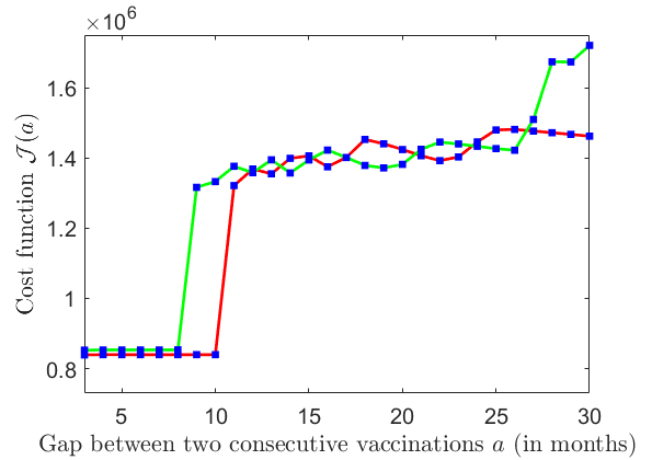
This critical observation suggests that excessively long intervals between vaccinations can be counterproductive, potentially leading to a surge in disease transmission and associated costs. This result shows that frequent vaccinations may not always be necessary and could potentially lead to diminishing returns, a phenomenon often referred to as hysteresis, whereas, an admissible larger gap between two consecutive vaccinations can effectively control the epidemic along with the minimal cost of vaccination campaign. This finding explains the significance of carefully determining the appropriate gap between two consecutive vaccination campaigns for effective epidemic control while minimizing economic burdens on a country or province.

A vaccination campaign focuses on two major aspects, the effectiveness of the vaccines and the rate of vaccination. These two factors can depend on the decision-makers. Thus it is important to understand the effect of vaccine efficacy and the rate of vaccination on the cost function. In figure (10), we plot the cost function $\mathcal{J}$ for two different vaccine efficacies. We notice that if the vaccine efficacy is less (red curve in Fig (10)) then the cost function remain at the minimum if the gap between the successive vaccination varies between 3 to 6 months. In contrast, if the vaccine efficacy is larger (blue curve in Fig (10)) then the cost function stays at a minimum if the gap between the successive vaccinations varies between 3 to 9 months. This observation suggests that highly effective vaccines may allow for more extended gaps between vaccinations, potentially reducing the frequency and cost of vaccination while still achieving effective epidemic control. Fig (11) shows the plot of the cost function $\mathcal{J}$ for two different vaccination rates. This figure shows that a higher vaccination rate provides more flexibility in increasing the gap between campaigns while still controlling the epidemic effectively and minimizing costs. The results are reminiscent of the recent experiences concerning COVID-19 vaccines [9]. This insight suggests that decision-makers should carefully consider both vaccine efficacy and vaccination rate when designing vaccination strategies to achieve cost-effective epidemic control.

The parameter $\kappa$ accounts for the existence of multiple strains. A higher value of $\kappa$ implies the co-existence of prominent strains with very different transmission rates. Figure (12) shows that a higher value of $\kappa$ provides less flexibility in increasing the gap between campaigns.

References

- [1] Roy M Anderson, Christophe Fraser, Azra C Ghani, Christl A Donnelly, Steven Riley, Neil M Ferguson, Gabriel M Leung, Tai H Lam, and Anthony J Hedley. Epidemiology, transmission dynamics and control of sars: the 2002–2003 epidemic. Philosophical Transactions of the Royal Society of London. Series B: Biological Sciences, 359(1447):1091–1105, 2004.
- [2] Weijia Xing, Gilles Hejblum, Gabriel M Leung, and Alain-Jacques Valleron. Anatomy of the epidemiological literature on the 2003 sars outbreaks in hong kong and toronto: a time-stratified review. PLoS medicine, 7(5):e1000272, 2010.
- [3] H Chen, GJD Smith, KS Li, J Wang, XH Fan, JM Rayner, D Vijaykrishna, JX Zhang, LJ Zhang, CT Guo, et al. Establishment of multiple sublineages of h5n1 influenza virus in asia: implications for pandemic control. Proceedings of the National Academy of Sciences, 103(8):2845–2850, 2006.
- [4] A Marm Kilpatrick, Aleksei A Chmura, David W Gibbons, Robert C Fleischer, Peter P Marra, and Peter Daszak. Predicting the global spread of h5n1 avian influenza. Proceedings of the National Academy of Sciences, 103(51):19368–19373, 2006.
- [5] Marc P Girard, John S Tam, Olga M Assossou, and Marie Paule Kieny. The 2009 a (h1n1) influenza virus pandemic: A review. Vaccine, 28(31):4895–4902, 2010.
- [6] Gavin JD Smith, Dhanasekaran Vijaykrishna, Justin Bahl, Samantha J Lycett, Michael Worobey, Oliver G Pybus, Siu Kit Ma, Chung Lam Cheung, Jayna Raghwani, Samir Bhatt, et al. Origins and evolutionary genomics of the 2009 swine-origin h1n1 influenza a epidemic. Nature, 459(7250):1122–1125, 2009.
- [7] Thomas R Frieden, Inger Damon, Beth P Bell, Thomas Kenyon, and Stuart Nichol. Ebola 2014—new challenges, new global response and responsibility. The New England Journal of Medicine, 371(13):1177–1180, 2014.
- [8] Edward C Holmes, Gytis Dudas, Andrew Rambaut, and Kristian G Andersen. The evolution of ebola virus: Insights from the 2013–2016 epidemic. Nature, 538(7624):193–200, 2016.
- [9] Amit K Chattopadhyay, Debajyoti Choudhury, Goutam Ghosh, Bidisha Kundu, and Sujit Kumar Nath. Infection kinetics of covid-19 and containment strategy. Scientific reports, 11(1):11606, 2021.
- [10] Javier Cachón-Zagalaz, María Sánchez-Zafra, Déborah Sanabrias-Moreno, Gabriel González-Valero, Amador J Lara-Sánchez, and María Luisa Zagalaz-Sánchez. Systematic review of the literature about the effects of the covid-19 pandemic on the lives of school children. Frontiers in psychology, 11:569348, 2020.
- [11] Fred Brauer. Compartmental models in epidemiology. In Mathematical epidemiology, pages 19–79. Springer, 2008.
- [12] Maia Martcheva. An introduction to mathematical epidemiology, volume 61. Springer, 2015.
- [13] Juliana Tolles and ThaiBinh Luong. Modeling epidemics with compartmental models. Jama, 323(24):2515–2516, 2020.
- [14] Herbert W Hethcote and P Van den Driessche. Some epidemiological models with nonlinear incidence. Journal of Mathematical Biology, 29(3):271–287, 1991.
- [15] Eli P Fenichel, Carlos Castillo-Chavez, M Graziano Ceddia, Gerardo Chowell, Paula A Gonzalez Parra, Graham J Hickling, Garth Holloway, Richard Horan, Benjamin Morin, Charles Perrings, et al. Adaptive human behavior in epidemiological models. Proceedings of the National Academy of Sciences, 108(15):6306–6311, 2011.
- [16] Derdei Bichara and Abderrahman Iggidr. Multi-patch and multi-group epidemic models: a new framework. Journal of Mathematical Biology, 77(1):107–134, 2018.
- [17] Daozhou Gao and Shigui Ruan. A multipatch malaria model with logistic growth populations. SIAM Journal on Applied Mathematics, 72(3):819–841, 2012.
- [18] Samiran Ghosh, Alonso Ogueda-Oliva, Aditi Ghosh, Malay Banerjee, and Padmanabhan Seshaiyer. Understanding the implications of under-reporting, vaccine efficiency and social behavior on the post-pandemic spread using physics informed neural networks: A case study of china. Plos one, 18(11):e0290368, 2023.
- [19] Cliff C Kerr, Robyn M Stuart, Dina Mistry, Romesh G Abeysuriya, Katherine Rosenfeld, Gregory R Hart, Rafael C Núñez, Jamie A Cohen, Prashanth Selvaraj, Brittany Hagedorn, et al. Covasim: an agent-based model of covid-19 dynamics and interventions. PLOS Computational Biology, 17(7):e1009149, 2021.
- [20] Nicolas Hoertel, Martin Blachier, Carlos Blanco, Mark Olfson, Marc Massetti, Marina Sánchez Rico, Frédéric Limosin, and Henri Leleu. A stochastic agent-based model of the sars-cov-2 epidemic in france. Nature medicine, 26(9):1417–1421, 2020.
- [21] Toshikazu Kuniya. Global stability analysis with a discretization approach for an age-structured multigroup sir epidemic model. Nonlinear Analysis Real World Application, 12(5):2640–2655, 2011.
- [22] Michael Y Li, Zhisheng Shuai, and Chuncheng Wang. Global stability of multi-group epidemic models with distributed delays. Journal of Mathematical Analysis and Applications, 361(1):38–47, 2010.
- [23] Lili Chang, Wei Gong, Zhen Jin, and Gui-Quan Sun. Sparse optimal control of pattern formations for an sir reaction-diffusion epidemic model. SIAM Journal on Applied Mathematics, 82(5):1764–1790, 2022.
- [24] Malay Banerjee, Samiran Ghosh, Piero Manfredi, and Alberto d’Onofrio. Spatio-temporal chaos and clustering induced by nonlocal information and vaccine hesitancy in the sir epidemic model. Chaos, Solitons & Fractals, 170:113339, 2023.
- [25] Jiandong Zhao, Lisha Wang, and Zhixia Han. Stability analysis of two new sirs models with two viruses. International Journal of Computer Mathematics, 95(10):2026–2035, 2018.
- [26] Ziyu Zhang, Xuehui Mei, Haijun Jiang, Xupeng Luo, and Yang Xia. Dynamical analysis of hyper-sir rumor spreading model. Applied Mathematics and Computation, 446:127887, 2023.
- [27] Fred Brauer, Carlos Castillo-Chavez, and Zhilan Feng. Mathematical models in epidemiology, volume 32. Springer, 2019.
- [28] Vincenzo Capasso. Mathematical structures of epidemic systems, volume 97. Springer Science & Business Media, 2008.
- [29] https://www.who.int/teams/immunization-vaccines-and-biologicals/diseases.
- [30] Y. et al Liu. Dosing interval strategies for two-dose covid-19 vaccination in 13 middle-income countries of europe: Health impact modelling and benefit-risk analysis. The Lancet Reg Health, 17:100381, 2022.
- [31] P. et al Dogra. A modeling-based approach to optimize covid-19 vaccine dosing schedules for improved protection. JCI Insight, 8(13):e169860, 2023.
- [32] F. et al Menegale. Evaluation of waning of sars-cov-2 vaccine–induced immunity: A systematic review and meta-analysis. JAMA Netw Open, 6(5):e2310650, 2023.
- [33] Samiran Ghosh, Vitaly Volpert, and Malay Banerjee. An epidemic model with time-distributed recovery and death rates. Bulletin of Mathematical Biology, 84(8):78, 2022.
- [34] Samiran Ghosh, Vitaly Volpert, and Malay Banerjee. An age-dependent immuno-epidemiological model with distributed recovery and death rates. Journal of Mathematical Biology, 86(2):21, 2023.
- [35] Samiran Ghosh, Malay Banerjee, and Vitaly Volpert. Immuno-epidemiological model-based prediction of further covid-19 epidemic outbreaks due to immunity waning. Mathematical Modelling of Natural Phenomena, 17:9, 2022.
- [36] https://in.mathworks.com/products/curvefitting.html.
- [37] Fawzi Ebrahim, Salah Tabal, Yosra Lamami, Inas M Alhudiri, Salah Edin El Meshri, Samira M Al Dwigen, Ramadan Arfa, Asma Alboeshi, Hafsa A Alemam, Fauzia Abuhtna, et al. Anti-sars-cov-2 igg antibodies after recovery from covid-19 or vaccination in libyan population: comparison of four vaccines. https://doi.org/10.1101/2022.02.18.22271130, 2022.
- [38] Ludek Berec, Martin Smid, Lenka Pribylova, Ondrej Majek, Tomas Pavlik, Jiri Jarkovsky, Milan Zajicek, Jakub Weiner, Tamara Barusova, and Jan Trnka. Real-life protection provided by vaccination, booster doses and previous infection against covid-19 infection, hospitalisation or death over time in the czech republic: a whole country retrospective view. https://doi.org/10.1101/2021.12.10.21267590, 2021.
- [39] Michael CW Chan, Kenrie PY Hui, John Ho, Man-chun Cheung, Ka-chun Ng, Rachel Ching, Ka-ling Lai, Tonia Kam, Haogao Gu, Ko-Yung Sit, et al. Sars-cov-2 omicron variant replication in human respiratory tract ex vivo. https://doi.org/10.21203/rs.3.rs-1189219/v1, 2021.
- [40] Billy J Quilty, Juliet RC Pulliam, and Carl AB Pearson. Test to release from isolation after testing positive for sars-cov-2. medRxiv, pages 2022–01, 2022.
- [41] Norman TJ Bailey. A statistical method of estimating the periods of incubation and infection of an infectious disease. Nature, 174:139–140, 1954.
- [42] Gerardo Chowell, James M Hyman, Luís MA Bettencourt, Carlos Castillo-Chavez, and H Nishiura. Mathematical and statistical estimation approaches in epidemiology. Springer, 2009.
- [43] Alun L Lloyd. Realistic distributions of infectious periods in epidemic models: changing patterns of persistence and dynamics. Theoretical population biology, 60(1):59–71, 2001.
- [44] https://www.who.int/teams/immunization-vaccines-and-biologicals/essential-programme-on-immunization/implementation/immunization-campaigns.
- [45] https://measlesrubellapartnership.org/.