跳到论文正文
W Papers独立论文阅读器 arXiv:2505.19945 论文正文 计算阅读时间 · 0%
引用这篇论文根据当前论文元数据生成,正式投稿前建议核对。


License: arXiv.org perpetual non-exclusive license
arXiv:2505.19945v2 [math.OC] 04 Jun 2025

Signed Angle Rigid Graphs for Network Localization and Formation Control

Jinpeng Huang and Gangshan Jing ††thanks: J.˜Huang and G.˜Jing are with School of Automation, Chongqing University, Chongqing 400044, China, 202313021067t@stu.cqu.edu.cn, jinggangshan@cqu.edu.cn
Abstract

Graph rigidity theory studies the capability of a graph embedded in the Euclidean space to constrain its global geometric shape via local constraints among nodes and edges, and has been widely exploited in network localization and formation control. In recent years, the traditional rigidity theory has been extended by considering new types of local constraints such as bearing, angle, ratio of distance, etc. Among them, the signed angle constraint has received extensive attention, since it is practically measurable and independent of the global coordinate frame. However, the relevant studies always consider special graph structures, which are sufficient but not necessary for signed angle rigidity. This paper presents a comprehensive combinatorial analysis in terms of graphs and angle index sets for signed angle rigidity. We show that Laman graphs equivalently characterize minimally signed angle rigid graphs. Moreover, we propose a method to construct the minimal set of signed angle constraints in a Laman graph to effectively ensure signed angle rigidity. These results are finally applied to distributed network localization and formation stabilization problems, respectively, where each agent only has access to signed angle measurements.

Index Terms: 
Graph rigidity theory, rigid formation control, network localization

I Introduction

The traditional graph rigidity theory studies the characterizability of a geometric shape by distance constraints among neighboring vertices in the graph, and has been widely employed in multi-agent coordination problems such as network localization [1, 2, 3] and formation control [4, 5, 6, 7, 8]. Inspired by this, rigidity theories based on other types of constraints (such as bearings [9, 10], angles [11, 12], ratio of distance [13], etc.) have been further developed to achieve network localization [14, 15, 16, 17, 18] and formation stabilization [9, 10, 11, 12, 19, 20, 13] via different sensing measurements. A geometric shape specified by different types of constraints may require different graphical conditions to ensure a unique shape [21]. As a result, different conditions on the network topology have been proposed depending on the type of measurements utilized.

In distance-based multi-agent coordination problems, infinitesimal distance rigidity has been adopted most widely since it has an equivalent rank condition on the rigidity matrix [22], which plays an essential role in the analysis of the gradient-based controller [23, 5, 24, 25]. However, infinitesimal distance rigidity does not guarantee the shape to be uniquely determined by distance constraints [26], which usually leads to local convergence of the controller. On the other hand, although global distance rigidity implies a unique shape, and has been favored in sensor network localization [1], it usually requires a large number of edges. Moreover, the formation controller achieving global convergence under globally rigid graphs is yet to be designed [27]. In [10], infinitesimal bearing rigidity was shown to share the same graphical conditions with infinitesimal distance rigidity (i.e., Laman graphs [28, 26]), while guaranteeing that the geometric shape is uniquely determined by bearings. Guided by this observation, the authors in [10, 16] proposed novel distributed protocols for bearing-based formation stabilization and sensor network localization. However, bearing constraints are associated with the global coordinate frame, which limits its applicability.

Recently, angle rigidity theory has garnered significant interest, as angle measurements are independent of the coordinate frame [14, 29, 30, 17, 18, 31], and an angle-constrained formation exhibits higher degrees of freedom than distance and bearing-based approaches [11, 12]. In [11], the authors established the equivalence between infinitesimal angle rigidity, infinitesimal bearing rigidity, and infinitesimal distance rigidity in the plane. However, it is unclear whether the shape of an infinitesimally angle rigid framework can be uniquely determined by angles. In [12], the authors reformulated angle rigidity theory by considering signed angle constraints. Unfortunately, the signed angle rigidity property was studied on angularities with predefined sets of angle constraints. Such a setting benefits for excluding redundant angles, but in the meanwhile, hinders the connection between the graph structure and the signed angle rigidity property.

In this paper, we study the conditions on graphs and the minimal set of signed angle constraints required to ensure signed angle rigidity and uniqueness of the shape. Similar issues related to angle rigidity theory have been investigated in the literature. In [32, 33], the authors explored the combinatorial conditions of angle rigidity. In [18, 12, 11], the authors reported a class of particular graphs which ensure a unique shape under angle constraints. Nevertheless, these works fail to characterize the equivalent graphical conditions for angle rigidity and the minimal set of angle constraints to guarantee a unique shape. Considering the large body of existing works in bearing rigidity theory, we believe that establishing the relationship between signed angle rigidity and bearing rigidity would be a worthwhile exploration.

Our contributions can be summarized as follows. (i). Enlightened by angle rigidity theory in [11, 12], we develop the signed angle rigidity theory in the context of frameworks, where all signed angles within the framework are utilized. Under this setting, it is shown that (infinitesimal, global) signed angle rigidity and (infinitesimal, global) bearing rigidity are completely equivalent, which implies that Laman graphs are exactly minimally signed angle rigid graphs; see Section II–III. (ii). Similarly to the bearing case, we prove that infinitesimal signed angle rigidity is sufficient and necessary for a framework to determine its shape uniquely; see Theorem 3. (iii). We provide a combinatorial analysis on the set of angle constraints and develop Algorithm 1 to generate a minimal angle index set (AIS) to characterize the rigidity property of a framework; see Section IV. (iv). Based on the theory developed, we solve the problems of network localization and formation stabilization, respectively, where each agent only has access to local signed angle measurements associated with its neighbors. Two distributed algorithms with global convergence guarantee are proposed, respectively, where the conditions on the sensing graph are much milder than those in [18, 11, 17, 12]; see Section V–VI.

This paper is structured as follows. Section II reviews bearing rigidity theory and introduces the concept of signed angle rigidity theory for frameworks in the plane. Section III establishes the equivalence on bearing rigidity and signed angle rigidity. Section IV provides a combinatorial analysis for minimal angle index sets. Section V-VI demonstrate the application of our results to network localization and formation stabilization. Section VII summarizes the entire paper.

Notations: In this paper, we denote the set of real numbers by ℝ{\mathbb{R}}; Let ℝd{\mathbb{R}}^{d} be the dd–dimensional Euclidean space; ∥⋅∥\|\cdot\| is the Euclidean norm; |A||A| indicates the number of the elements in the set AA; X⊤X^{\top} denotes the transpose of the matrix XX; ⊗\otimes is the Kronecker product; Null(XX) and rank(XX) are defined as the null space and rank of the matrix XX, respectively; Define In∈ℝn×nI_{n}\in\mathbb{R}^{n\times n} as the identity matrix; 1n≜(1,⋯,1)⊤\textbf{1}_{n}\triangleq(1,\cdots,1)^{\top}; Denote A\BA\backslash B as the set that consists of the elements belonging to AA but not to BB; Denote ℛo​(θ)\mathscr{R}_{o}(\theta) as the 2-dimensional rotation matrix associated with θ∈[0,2​π)\theta\in[0,2\pi); For a vector x∈ℝ2x\in{\mathbb{R}}^{2}, x⟂≜ℛo​(π2)​xx^{\perp}\triangleq\mathscr{R}_{o}(\frac{\pi}{2})x; For Xi∈ℝa×b,i=1,⋯,qX_{i}\in{\mathbb{R}}^{a\times b},i=1,\cdots,q, diag(Xi)≜\left(X_{i}\right)\triangleq blockdiag{X1,⋯,Xq}∈ℝq​a×q​b\left\{X_{1},\cdots,X_{q}\right\}\in{\mathbb{R}}^{qa\times qb}.

We consider the undirected graph 𝒢≜(𝒱,ℰ){\mathcal{G}}\triangleq\left(\mathcal{V},\mathcal{E}\right), where 𝒱≜{1,⋯,n}\mathcal{V}\triangleq\left\{1,\cdots,n\right\} is the vertex set satisfying n≥3n\geq 3, ℰ⊆𝒱×𝒱\mathcal{E}\subseteq\mathcal{V}\times\mathcal{V} is the edge set, and (i,j)∈ℰ(i,j)\in\mathcal{E} is equivalent to (j,i)∈ℰ(j,i)\in\mathcal{E} in 𝒢\mathcal{G}. The set of neighbors of the vertex jj in 𝒢\mathcal{G} is denoted by 𝒩𝒢j≜{j∈𝒱:(j,i)∈ℰ}\mathcal{N}^{j}_{\mathcal{G}}\triangleq\left\{j\in\mathcal{V}:(j,i)\in\mathcal{E}\right\}. If 𝒢\mathcal{G} is clear from the context, we simply denote 𝒩𝒢j\mathcal{N}^{j}_{\mathcal{G}} by 𝒩j\mathcal{N}_{j}. The undirected complete graph with the same number of nodes as 𝒢\mathcal{G} is denoted by 𝒦\mathcal{K}. A graph 𝒢¯≜(𝒱¯,ℰ¯)\bar{\mathcal{G}}\triangleq(\bar{\mathcal{V}},\bar{\mathcal{E}}) is said to be a subgraph of 𝒢\mathcal{G} if 𝒱¯⊆𝒱\bar{\mathcal{V}}\subseteq\mathcal{V} and ℰ¯⊆(𝒱¯×𝒱¯)​⋂ℰ\bar{\mathcal{E}}\subseteq(\bar{\mathcal{V}}\times\bar{\mathcal{V}})\bigcap\mathcal{E}. A subgraph is said to be a spanning subgraph if it is connected and 𝒱¯=𝒱\bar{\mathcal{V}}=\mathcal{V}.

Given an undirected graph 𝒢\mathcal{G}, an undirected path between l1∈𝒱l_{1}\in\mathcal{V} and lnP∈𝒱l_{n_{P}}\in\mathcal{V} is a sequence of edges of the form (l1,l2)(l_{1},l_{2}),…,(lnP−1,lnP)\dots,(l_{n_{P}-1},l_{n_{P}}). In this paper, for the sake of analysis, we use the subgraph 𝒫≜(𝒱P,ℰP)\mathcal{P}\triangleq(\mathcal{V}_{P},\mathcal{E}_{P}) to represent the corresponding undirected path, where 𝒱P≜{l1,…,lnP}⊆𝒱\mathcal{V}_{P}\triangleq\{l_{1},\dots,l_{n_{P}}\}\subseteq\mathcal{V} and ℰP≜{(l1,l2),…,(lnP−1,lnP)}⊆ℰ\mathcal{E}_{P}\triangleq\{(l_{1},l_{2}),\dots,(l_{n_{P}-1},l_{n_{P}})\}\subseteq\mathcal{E}. An undirected cycle is an undirected path in 𝒢\mathcal{G} that starts and ends at the same node. We use the subgraph 𝒞≜(𝒱C,ℰC)\mathcal{C}\triangleq(\mathcal{V}_{C},\mathcal{E}_{C}) to represent the corresponding undirected cycle, where 𝒱C≜{l1,…,lnP}⊆𝒱\mathcal{V}_{C}\triangleq\{l_{1},\dots,l_{n_{P}}\}\subseteq\mathcal{V} and ℰC≜{(l1,l2),…,(lnP−1,lnP),(lnP,l1)}⊆ℰ\mathcal{E}_{C}\triangleq\{(l_{1},l_{2}),\dots,(l_{n_{P}-1},l_{n_{P}}),(l_{n_{P}},l_{1})\}\subseteq\mathcal{E}.

II Preliminaries

In this section, we briefly review some background on bearing rigidity theory [10], define signed angle rigidity in the context of frameworks, and introduce some concepts related to the index set of angle constraints.

II-A Graph Rigidity Theory

To begin with, we introduce some important notions in rigidity theory based on a smooth rigidity function. Given different smooth rigidity functions, different rigidity theories can be developed accordingly, e.g., bearing rigidity theory and signed angle rigidity theory.

A framework (𝒢,p)(\mathcal{G},p) in ℝd\mathbb{R}^{d} is characterized by an undirected graph 𝒢\mathcal{G} and a configuration p=(p1⊤,⋯,pn⊤)⊤∈ℝd​np=\left(p^{\top}_{1},\cdots,p^{\top}_{n}\right)^{\top}\in\mathbb{R}^{dn}, where pip_{i} is the coordinate mapped to the vertex i,i=1,⋯,ni,i=1,\cdots,n with the assumption that pi≠pjp_{i}\neq p_{j} for any j∈{1,⋯,n}\{i}j\in\{1,\cdots,n\}\backslash\{i\}. If p1,⋯,pnp_{1},\cdots,p_{n} do not belong to a hyperplane of ℝd\mathbb{R}^{d}, we refer pp to be non-degenerate, and the framework (𝒢,p)(\mathcal{G},p) is said to be a non-degenerate framework. Given a spanning subgraph 𝒢¯\bar{\mathcal{G}} of 𝒢\mathcal{G}, (𝒢¯,p)(\bar{\mathcal{G}},p) is said to be the spanning subframework of (𝒢,p)(\mathcal{G},p).

Given a framework (𝒢,p)(\mathcal{G},p), a smooth rigidity function r𝒢​(⋅):ℝd​n→ℝsr_{\mathcal{G}}(\cdot):\mathbb{R}^{dn}\rightarrow\mathbb{R}^{s} is a function of p∈ℝd​np\in\mathbb{R}^{dn}, and each entry of r𝒢​(p)r_{\mathcal{G}}(p) corresponds to a constraint in (𝒢,p)(\mathcal{G},p), here ss is the number of constraints. Based on r𝒢​(⋅)r_{\mathcal{G}}(\cdot), a series of relevant concepts can be given.

Definition 1

In ℝd\mathbb{R}^{d}, a framework (𝒢,p)(\mathcal{G},p) is said to be rigid if there exists a neighborhood UpU_{p} of pp, such that for any q∈r𝒢−1​(r𝒢​(p))​⋂Upq\in r^{-1}_{\mathcal{G}}\left(r_{\mathcal{G}}(p)\right)\bigcap U_{p}, it always holds r𝒦​(q)=r𝒦​(p)r_{\mathcal{K}}(q)=r_{\mathcal{K}}(p).

Definition 2

In ℝd\mathbb{R}^{d}, a framework (𝒢,p)(\mathcal{G},p) is said to be globally rigid if r𝒢−1​(r𝒢​(p))=r𝒦−1​(r𝒦​(p))r^{-1}_{\mathcal{G}}\left(r_{\mathcal{G}}(p)\right)=r^{-1}_{\mathcal{K}}\left(r_{\mathcal{K}}(p)\right).

Definition 3

In ℝd\mathbb{R}^{d}, a rigid framework (𝒢,p)(\mathcal{G},p) is said to be minimally rigid if there does not exist any rigid spanning subframework (𝒢¯,p)(\bar{\mathcal{G}},p) of (𝒢,p)(\mathcal{G},p) such that |ℰ¯|<|ℰ||\bar{\mathcal{E}}|<|\mathcal{E}|.

By definition, global rigidity implies rigidity.

An instantaneously continuous motion p˙≜v=(v1⊤,⋯,vn⊤)⊤\dot{p}\triangleq v=(v^{\top}_{1},\cdots,v^{\top}_{n})^{\top} is said to be an infinitesimal motion if it preserves the invariance of r𝒢​(p)r_{\mathcal{G}}(p), i.e.,

r˙𝒢​(p)=∂r𝒢​(p)∂p​v=0.\displaystyle\dot{r}_{\mathcal{G}}(p)=\frac{\partial r_{\mathcal{G}}(p)}{\partial p}v=0. (1)

A motion is said to be trivial if it preserves rigidity for any framework. For example, if each entry of r𝒢​(p)r_{\mathcal{G}}(p) is a distance, i.e., ‖pi−pj‖\|p_{i}-p_{j}\|, then the trivial motions consist of uniform rotations and translations of the whole framework [34].

Definition 4

In ℝd\mathbb{R}^{d}, a framework (𝒢,p)(\mathcal{G},p) is said to be infinitesimally rigid if all of its infinitesimal motions are trivial.

The rigidity matrix is defined as R⁡(p)≜∂r𝒢​(p)∂pR(p)\triangleq\frac{\partial r_{\mathcal{G}}(p)}{\partial p}. Then, (1) can be rewritten as r˙𝒢​(p)=R⁡(p)​p˙=0\dot{r}_{\mathcal{G}}(p)=R(p)\dot{p}=0. It can be obtained that a framework (𝒢,p)(\mathcal{G},p) in ℝd\mathbb{R}^{d} is infinitesimally rigid if and only if rank⁡(R⁡(p))=d​n−T\rank(R(p))=dn-T, where TT is the dimension of the space spanned by trivial motions.

So far, we have introduced some relevant rigidity concepts based on a given rigidity function. Throughout this paper, we mainly focus on the case in ℝ2\mathbb{R}^{2}. In following subsections, we will introduce two specific rigidity functions, i.e., bearing rigidity function and signed angle rigidity function, based on which similar rigidity concepts can be induced naturally.

Refer to caption
Fig. 1: Example of the bearing and the signed angle among three agents.

II-B Bearing Rigidity

Given a framework (𝒢,p)(\mathcal{G},p) in ℝ2\mathbb{R}^{2}, according to [10], the bearing rigidity function is described as:

B𝒢​(p)=(⋯,bj​i⊤,⋯)⊤,(j,i)∈ℰ,\displaystyle B_{\mathcal{G}}(p)=\left(\cdots,b^{\top}_{ji},\cdots\right)^{\top},(j,i)\in\mathcal{E}, (2)

where bj​i≜bj​i​(p)=pi−pj‖pi−pj‖∈ℝ2b_{ji}\triangleq b_{ji}(p)=\frac{p_{i}-p_{j}}{\|p_{i}-p_{j}\|}\in\mathbb{R}^{2} is the bearing vector from pjp_{j} to pip_{i} (see Fig. 1). The bearing rigidity matrix is

RB​(p)≜diag⁡(Pj​i‖ej​i‖)​H¯∈ℝ2​|ℰ|×2​n,\displaystyle R_{B}(p)\triangleq{\rm diag}\left(\frac{P_{ji}}{\|e_{ji}\|}\right)\bar{H}\in\mathbb{R}^{2|\mathcal{E}|\times 2n}, (3)

where ej​i≜pi−pje_{ji}\triangleq p_{i}-p_{j}, Pj​i≜P⁡(bj​i)=I2−bj​i​bj​i⊤P_{ji}\triangleq P(b_{ji})=I_{2}-b_{ji}b^{\top}_{ji} is an orthogonal projection matrix projecting any vector onto the orthogonal space of bj​ib_{ji}, H¯≜(H⊗I2)\bar{H}\triangleq\left(H\otimes I_{2}\right), H=[hj​i]H=\left[h_{ji}\right] is the incidence matrix whose rows are indexed by edges of 𝒢\mathcal{G} and columns are indexed by vertices of 𝒢\mathcal{G} with an orientation: hj​i=1h_{ji}=1 if vertex ii is the end of the jjth edge, hj​i=−1h_{ji}=-1 if vertex ii is the start of the jjth edge, and hj​i=0h_{ji}=0 otherwise.

Since bearing-preserving motions of a framework in ℝ2\mathbb{R}^{2} include 2-dimensional uniform translations and 1-dimensional uniform scalings [10], a framework is infinitesimally bearing rigid if and only if rank⁡(RB​(p))=2​n−3\rank(R_{B}(p))=2n-3.

II-C Signed Angle Rigidity

Given a framework (𝒢,p)(\mathcal{G},p) in ℝ2\mathbb{R}^{2}, according to [12], the signed angle rigidity function is defined as:

S𝒢​(p)=(⋯,αi​j​k,⋯)⊤,(i,j,k)∈𝒯𝒢,\displaystyle S_{\mathcal{G}}(p)=\left(\cdots,\alpha_{ijk},\cdots\right)^{\top},(i,j,k)\in\mathcal{T}_{\mathcal{G}}, (4)

where αi​j​k≜αi​j​k​(p)∈[0,2​π)\alpha_{ijk}\triangleq\alpha_{ijk}(p)\in[0,2\pi) describes the signed angle from bj​ib_{ji} to bj​kb_{jk} in the counter-clockwise direction (see Fig. 1), and is computed by

αi​j​k\displaystyle\alpha_{ijk} ={arccos⁡(bj​k⊤​bj​i)if​bj​k⊤​bj​i⊥≥0,2​π−arccos⁡(bj​k⊤​bj​i)otherwise,\displaystyle=\left\{\begin{array}[]{ll}{\rm arccos}\left(b^{\top}_{jk}b_{ji}\right)&{\rm if}~b^{\top}_{jk}b^{\bot}_{ji}\geq 0,\\ 2\pi-{\rm arccos}\left(b^{\top}_{jk}b_{ji}\right)&{\rm otherwise},\end{array}\right.

𝒯𝒢={(i,j,k)∈𝒱3:(j,i),(j,k)∈ℰ,i<k}\mathcal{T}_{\mathcal{G}}=\left\{(i,j,k)\in\mathcal{V}^{3}:(j,i),(j,k)\in\mathcal{E},i<k\right\} is a set indexing all signed angles in (𝒢,p)(\mathcal{G},p), here (i,j,k)(i,j,k) corresponds to the signed angle αi​j​k\alpha_{ijk}. By differentiating S𝒢​(p)S_{\mathcal{G}}(p) w.r.t. pp, one has the signed angle rigidity matrix:

RS𝒯𝒢​(p)≜diag⁡(−1sin​αi​j​k)​Rb​(p)​RB​(p)∈ℝ|𝒯𝒢|×2​n,\displaystyle R^{\mathcal{T}_{\mathcal{G}}}_{S}(p)\triangleq{\rm diag}\left(-\frac{1}{{\rm sin}\alpha_{ijk}}\right)R_{b}(p)R_{B}(p)\in\mathbb{R}^{|\mathcal{T}_{\mathcal{G}}|\times 2n}, (8)

where RB​(p)R_{B}(p) is the bearing rigidity matrix and Rb​(p)∈ℝ|𝒯𝒢|×2​|ℰ|R_{b}(p)\in\mathbb{R}^{|\mathcal{T}_{\mathcal{G}}|\times 2|\mathcal{E}|} can be written as

⋯bj​i⋯bj​k⋯⋯( ⋯⋯⋯⋯⋯) ⋯⋯⋯⋯⋯⋯αi​j​k𝟎bj​k⊤𝟎bj​i⊤𝟎⋯⋯⋯⋯⋯⋯⋯⋯⋯⋯⋯⋯\displaystyle\bordermatrix{&\cdots&b_{ji}&\cdots&b_{jk}&\cdots\cr\hskip 14.22636pt\cdots&\cdots&\cdots&\cdots&\cdots&\cdots\cr\hskip 14.22636pt\cdots&\cdots&\cdots&\cdots&\cdots&\cdots\cr\hskip 8.53581pt\alpha_{ijk}&\boldsymbol{0}&b_{jk}^{\top}&\boldsymbol{0}&b_{ji}^{\top}&\boldsymbol{0}\cr\hskip 14.22636pt\cdots&\cdots&\cdots&\cdots&\cdots&\cdots\cr\hskip 14.22636pt\cdots&\cdots&\cdots&\cdots&\cdots&\cdots}

whose rows are indexed by 𝒯𝒢\mathcal{T}_{\mathcal{G}} and columns are indexed by the edges of 𝒢\mathcal{G}.

It should be noted that the existence of sin⁡αi​j​k=0\sin\alpha_{ijk}=0 in (8) seems to render the signed angle rigidity matrix RS𝒯𝒢​(p)R^{\mathcal{T}_{\mathcal{G}}}_{S}(p) invalid. In order to eliminate this singularity, we derive another expression for the signed angle rigidity matrix.

Lemma 1

The signed angle rigidity matrix (8) can be expressed as

RS𝒯𝒢​(p)=R¯𝒯𝒢​(p)​H¯,\displaystyle R^{\mathcal{T}_{\mathcal{G}}}_{S}(p)=\bar{R}_{\mathcal{T}_{\mathcal{G}}}(p)\bar{H}, (9)

where R¯𝒯𝒢​(p)∈ℝ|𝒯𝒢|×2​|ℰ|\bar{R}_{\mathcal{T}_{\mathcal{G}}}(p)\in\mathbb{R}^{|\mathcal{T}_{\mathcal{G}}|\times 2|\mathcal{E}|} is

⋯bj​i⋯bj​k⋯⋯( ⋯⋯⋯⋯⋯) ⋯⋯⋯⋯⋯⋯αi​j​k𝟎bj​i⊤​ℛo​(π2)‖ej​i‖𝟎−bj​k⊤​ℛo​(π2)‖ej​k‖𝟎⋯⋯⋯⋯⋯⋯⋯⋯⋯⋯⋯⋯.\displaystyle\bordermatrix{&\cdots&b_{ji}&\cdots&b_{jk}&\cdots\cr\hskip 14.22636pt\cdots&\cdots&\cdots&\cdots&\cdots&\cdots\cr\hskip 14.22636pt\cdots&\cdots&\cdots&\cdots&\cdots&\cdots\cr\hskip 8.53581pt\alpha_{ijk}&\boldsymbol{0}&\frac{b_{ji}^{\top}\mathscr{R}_{o}(\frac{\pi}{2})}{\|e_{ji}\|}&\boldsymbol{0}&-\frac{b_{jk}^{\top}\mathscr{R}_{o}(\frac{\pi}{2})}{\|e_{jk}\|}&\boldsymbol{0}\cr\hskip 14.22636pt\cdots&\cdots&\cdots&\cdots&\cdots&\cdots\cr\hskip 14.22636pt\cdots&\cdots&\cdots&\cdots&\cdots&\cdots}.
Proof:

See Appendix VIII-A. ∎

In bearing rigidity theory, a framework is infinitesimally rigid if and only if the rank of the related rigidity matrix is 2​n−32n-3. One may question if there is a similar conclusion in signed angle rigidity theory. In [12], the authors proposed the signed angle rigidity theory for angularities and showed that an angularity is infinitesimally signed angle rigid if and only if rank⁡(RS𝒯¯𝒢​(p))=2​n−4\rank(R^{\bar{\mathcal{T}}_{\mathcal{G}}}_{S}(p))=2n-4, where an angularity involves a pre-designed subset 𝒯¯𝒢⊆𝒯𝒢\bar{\mathcal{T}}_{\mathcal{G}}\subseteq\mathcal{T}_{\mathcal{G}} specifying constrained signed angles with the assumption that sin⁡αi​j​k≠0\sin\alpha_{ijk}\neq 0 for (i,j,k)∈𝒯¯𝒢(i,j,k)\in\bar{\mathcal{T}}_{\mathcal{G}}.

In order to build connections with bearing rigidity theory in a unified architecture, we utilize all the signed angles in the framework to study the signed angle rigidity property without imposing any assumptions on these signed angle constraints. That is, given a framework (𝒢,p)(\mathcal{G},p), it becomes certain whether there exists a subset 𝒯¯𝒢⊆𝒯𝒢\bar{\mathcal{T}}_{\mathcal{G}}\subseteq\mathcal{T}_{\mathcal{G}} that validates (infinitesimal, global) signed angle rigidity.

To better discuss the existence of such a subset, we will propose several definitions in the following subsection.

II-D Angle Index Set and Angle Index Graph

Given a graph 𝒢\mathcal{G}, we refer to a subset 𝒯¯𝒢⊆𝒯𝒢\bar{\mathcal{T}}_{\mathcal{G}}\subseteq\mathcal{T}_{\mathcal{G}} as the angle index set (AIS) and present the following definitions.

Definition 5

For a given framework (𝒢,p)(\mathcal{G},p), an AIS 𝒯¯𝒢⊆𝒯𝒢\bar{\mathcal{T}}_{\mathcal{G}}\subseteq\mathcal{T}_{\mathcal{G}} is said to be the global angle index set (GAIS) if for any q∈ℝ2​nq\in\mathbb{R}^{2n} such that αi​j​k​(q)=αi​j​k​(p),(i,j,k)∈𝒯¯𝒢\alpha_{ijk}(q)=\alpha_{ijk}(p),(i,j,k)\in\bar{\mathcal{T}}_{\mathcal{G}}, it always holds that S𝒢​(q)=S𝒢​(p)S_{\mathcal{G}}(q)=S_{\mathcal{G}}(p).

By definition, 𝒯𝒢\mathcal{T}_{\mathcal{G}} is always a GAIS.

Definition 6

For a given framework (𝒢,p)(\mathcal{G},p), an AIS 𝒯𝒢∗⊆𝒯𝒢\mathcal{T}^{*}_{\mathcal{G}}\subseteq\mathcal{T}_{\mathcal{G}} is said to be a regular angle index set (RAIS) if rank⁡(RS𝒯𝒢∗​(p))=rank⁡(RS𝒯𝒢​(p))\rank(R^{\mathcal{T}^{*}_{\mathcal{G}}}_{S}(p))=\rank(R_{S}^{\mathcal{T}_{\mathcal{G}}}(p)).

Definition 7

Given an RAIS 𝒯𝒢∗\mathcal{T}^{*}_{\mathcal{G}}, if there does not exist another RAIS with fewer elements than 𝒯𝒢∗\mathcal{T}^{*}_{\mathcal{G}}, then it is said to be a minimal RAIS. The same goes for GAIS.

Since an angular constraint is related to two edges in the framework, it is necessary to evaluate an AIS from the perspective of the edge set. We use the Hash function H⁡(i,j,|𝒱|)=(min⁡({i,j})−1)×|𝒱|+max⁡({i,j})H(i,j,|\mathcal{V}|)=(\min(\{i,j\})-1)\times|\mathcal{V}|+\max(\{i,j\}) to encode the edge (i,j)(i,j) of a given graph 𝒢\mathcal{G} sequentially, and propose the following definitions

Definition 8 (Angle Index Graph)

Given a graph 𝒢\mathcal{G} and an AIS 𝒯¯𝒢⊆𝒯𝒢\bar{\mathcal{T}}_{\mathcal{G}}\subseteq\mathcal{T}_{\mathcal{G}}, the undirected angle index graph is denoted by 𝒢A​(𝒯¯𝒢)=(𝒱A​(𝒢),ℰA​(𝒯¯𝒢))\mathcal{G}_{A}(\bar{\mathcal{T}}_{\mathcal{G}})=\left(\mathcal{V}_{A}(\mathcal{G}),\mathcal{E}_{A}(\bar{\mathcal{T}}_{\mathcal{G}})\right), where the vertex set is 𝒱A​(𝒢)={ai​j=H⁡(i,j,|𝒱|):(i,j)∈ℰ}\mathcal{V}_{A}(\mathcal{G})=\{a_{ij}=H(i,j,|\mathcal{V}|):(i,j)\in\mathcal{E}\}, ai​j∈𝒱A​(𝒢)a_{ij}\in\mathcal{V}_{A}(\mathcal{G}) is equivalent to aj​i∈𝒱A​(𝒢)a_{ji}\in\mathcal{V}_{A}(\mathcal{G}), and the edge set is ℰA(𝒯¯𝒢)={(aj​i,aj​k):aj​i,aj​k∈𝒱A(𝒢),(i,j,k)∈𝒯¯𝒢}\mathcal{E}_{A}(\bar{\mathcal{T}}_{\mathcal{G}})=\{(a_{ji},a_{jk}):a_{ji},a_{jk}\in\mathcal{V}_{A}(\mathcal{G}),(i,j,k)\in\bar{\mathcal{T}}_{\mathcal{G}}\}.

If 𝒢\mathcal{G} and 𝒯¯𝒢\bar{\mathcal{T}}_{\mathcal{G}} are clear from the context, we simply denote 𝒢A​(𝒯¯𝒢)=(𝒱A​(𝒢),ℰA​(𝒯¯𝒢))\mathcal{G}_{A}(\bar{\mathcal{T}}_{\mathcal{G}})=\left(\mathcal{V}_{A}(\mathcal{G}),\mathcal{E}_{A}(\bar{\mathcal{T}}_{\mathcal{G}})\right) as 𝒢A=(𝒱A,ℰA)\mathcal{G}_{A}=\left(\mathcal{V}_{A},\mathcal{E}_{A}\right).

Definition 9

Given a graph 𝒢\mathcal{G} and an AIS 𝒯¯𝒢⊆𝒯𝒢\bar{\mathcal{T}}_{\mathcal{G}}\subseteq\mathcal{T}_{\mathcal{G}}, 𝒯¯𝒢\bar{\mathcal{T}}_{\mathcal{G}} is said to be angle connected if the angle index graph (𝒱A​(𝒢),ℰA​(𝒯¯𝒢))\left(\mathcal{V}_{A}(\mathcal{G}),\mathcal{E}_{A}(\bar{\mathcal{T}}_{\mathcal{G}})\right) is connected.

Refer to caption
Fig. 2: (a) A non-infinitesimally signed angle rigid framework (𝒢,p)(\mathcal{G},p) and an angle connected set 𝒯¯𝒢={(2,1,3),(1,2,6),(1,3,2),(2,3,4),(3,4,5),(5,4,6),(1,5,4),(4,6,5)}\bar{\mathcal{T}}_{\mathcal{G}}=\{(2,1,3),(1,2,6),(1,3,2),(2,3,4),(3,4,5),(\\ 5,4,6),(1,5,4),(4,6,5)\}, where the red arrows stand for non-trivial infinitesimal signed angle motions. (b) The angle index graph of 𝒢\mathcal{G} and 𝒯¯𝒢\bar{\mathcal{T}}_{\mathcal{G}}, where vertex 1212 satisfies 12=a26=H⁡(2,6,6)=(2−1)×6+612=a_{26}=H(2,6,6)=(2-1)\times 6+6.

Note that 𝒢A​(𝒯¯𝒢)=(𝒱A​(𝒢),ℰA​(𝒯¯𝒢))\mathcal{G}_{A}(\bar{\mathcal{T}}_{\mathcal{G}})=\left(\mathcal{V}_{A}(\mathcal{G}),\mathcal{E}_{A}(\bar{\mathcal{T}}_{\mathcal{G}})\right) is formed by mapping the edge (i,j)∈ℰ(i,j)\in\mathcal{E} to the vertex in 𝒢A​(𝒯¯𝒢)\mathcal{G}_{A}(\bar{\mathcal{T}}_{\mathcal{G}}) and the index (i,j,k)∈𝒯¯𝒢(i,j,k)\in\bar{\mathcal{T}}_{\mathcal{G}} to the undirected edge in 𝒢A​(𝒯¯𝒢)\mathcal{G}_{A}(\bar{\mathcal{T}}_{\mathcal{G}}), respectively. Furthermore, for a given graph 𝒢\mathcal{G}, an angle index graph 𝒢A​(𝒯¯𝒢)\mathcal{G}_{A}(\bar{\mathcal{T}}_{\mathcal{G}}) can uniquely deduce an AIS. Fig. 2 illustrates an example of the angle connected set 𝒯¯𝒢⊆𝒯𝒢\bar{\mathcal{T}}_{\mathcal{G}}\subseteq\mathcal{T}_{\mathcal{G}}, where the angular constraints between edges and their interrelationships are visually presented.

Throughout this paper, we use shorthands SAR, GSAR, and ISAR for signed angle rigid (signed angle rigidity), globally signed angle rigid (global signed angle rigidity), and infinitesimally signed angle rigid (infinitesimal signed angle rigidity), respectively. Similarly, BR, GBR, and IBR are shorthands for corresponding concepts in bearing rigidity theory.

III Graphs for Signed Angle Rigidity

In this section, we establish the equivalence between signed angle constraints and bearing constraints in the sense that a framework (𝒢,p)(\mathcal{G},p) is IBR, GBR, and BR if and only if it is ISAR, GSAR, and SAR, respectively. Based on these relationships, we derive necessary and sufficient graphical conditions for signed angle rigidity.

III-A Equivalence on IBR and ISAR

In [12], the authors showed that if sin⁡αi​j​k≠0,(i,j,k)∈𝒯𝒢\sin\alpha_{ijk}\neq 0,(i,j,k)\in\mathcal{T}_{\mathcal{G}}, the null space of the signed angle rigidity matrix RS𝒯𝒢​(p)R^{\mathcal{T}_{\mathcal{G}}}_{S}(p) contains the following three linear spaces:

ℳs\displaystyle\mathcal{M}_{s} ≜\displaystyle\hskip-5.69054pt\triangleq\hskip-5.69054pt span​{p},\displaystyle{\rm span}\{p\}, (10)
ℳr\displaystyle\mathcal{M}_{r} ≜\displaystyle\hskip-5.69054pt\triangleq\hskip-5.69054pt span⁡{(In⊗ℛo​(π2))​p},\displaystyle{\rm span}\left\{(I_{n}\otimes\mathscr{R}_{o}(\frac{\pi}{2}))p\right\}, (11)
ℳt\displaystyle\mathcal{M}_{t} ≜\displaystyle\hskip-5.69054pt\triangleq\hskip-5.69054pt span⁡{1n⊗(1,0)⊤,1n⊗(0,1)⊤}.\displaystyle{\rm span}\left\{\textbf{1}_{n}\otimes(1,0)^{\top},\textbf{1}_{n}\otimes(0,1)^{\top}\right\}. (12)

According to Lemma 1, it can be verified that the result remains valid even when there exist triplets (i,j,k)∈𝒯𝒢(i,j,k)\in\mathcal{T}_{\mathcal{G}} satisfying sin⁡αi​j​k=0\sin\alpha_{ijk}=0. Therefore, the following lemma can be derived from Definition 4 naturally, which implies that the trivial infinitesimal signed angle motions of a framework in ℝ2\mathbb{R}^{2} include 2-dimensional uniform translations, 1-dimensional uniform scalings, and 1-dimensional uniform rotations.

Lemma 2

In ℝ2\mathbb{R}^{2}, a framework (𝒢,p)(\mathcal{G},p) is ISAR if and only if Null⁡(RS𝒯𝒢​(p))=ℳs​⋃ℳr​⋃ℳt\Null(R^{\mathcal{T}_{\mathcal{G}}}_{S}(p))=\mathcal{M}_{s}\bigcup\mathcal{M}_{r}\bigcup\mathcal{M}_{t}.

As shown in Fig. 2(a), the framework is not ISAR since there exists a non-trivial infinitesimal signed angle motion. Lemma 2 also indicates that a framework (𝒢,p)(\mathcal{G},p) in ℝ2\mathbb{R}^{2} is ISAR if and only if rank⁡(RS𝒯𝒢​(p))\rank(R^{\mathcal{T}_{\mathcal{G}}}_{S}(p)) = 2​n−42n-4. Next, we present a key property of ISAR frameworks.

Theorem 1

In ℝ2\mathbb{R}^{2}, a framework (𝒢,p)(\mathcal{G},p) is ISAR if and only if it is IBR.

Proof:

See Appendix VIII-B. ∎

Theorem 1 implies that the conditions on the framework for bearing constraints and signed angle constraints to exclude non-trivial infinitesimal motions are the same. In [10], it has been shown that the shape of an IBR framework can always be uniquely fixed by all bearings among neighboring nodes. However, Theorem 1 does not imply that an ISAR framework can fix its shape by using all its angular information. To seek the conditions on frameworks for signed angles to constrain a shape uniquely, we study the relationship between GSAR and GBR in the next subsection.

III-B Equivalence on GSAR and GBR

In this subsection, we establish the equivalence among GSAR, GBR, SAR and BR. Before that, we propose a graphical condition, under which signed angle constraints are equivalent to bearing constraints regardless of uniform rotations.

Lemma 3

Given a connected graph 𝒢\mathcal{G} and two configurations p,q∈ℝ2​np,q\in\mathbb{R}^{2n}, S𝒢​(q)=S𝒢​(p)S_{\mathcal{G}}(q)=S_{\mathcal{G}}(p) if and only if B𝒢​(q)=(In⊗ℛo​(θ))​B𝒢​(p)B_{\mathcal{G}}(q)=\left(I_{n}\otimes\mathscr{R}_{o}(\theta)\right)B_{\mathcal{G}}(p) for some θ∈[0,2​π)\theta\in[0,2\pi).

Proof:

See Appendix VIII-C. ∎

Lemma 3 implies that, despite being measured in different local coordinate frames, signed angle constraints are able to function as bearing constraints in a certain coordinate frame as long as the graph is connected. This is an interesting property with great potential in coordinate-free formation control and network localization, but surprisingly, not found in the literature.

Now we are ready to show the equivalence between GBR and GSAR.

Theorem 2

A framework (𝒢,p)(\mathcal{G},p) in ℝ2\mathbb{R}^{2} is BR (GBR) if and only if it is SAR (GSAR).

Proof:

Sufficiency. Suppose (𝒢,p)(\mathcal{G},p) is SAR. Then, there exists a neighborhood UpU_{p} of pp such that for any q∈S𝒢−1​(S𝒢​(p))​⋂Upq\in S^{-1}_{\mathcal{G}}\left(S_{\mathcal{G}}(p)\right)\bigcap U_{p}, it always holds S𝒦​(q)=S𝒦​(p)S_{\mathcal{K}}(q)=S_{\mathcal{K}}(p). It suffices to show that for this UpU_{p}, consider any q∈B𝒢−1​(B𝒢​(p))​⋂Upq\in B^{-1}_{\mathcal{G}}(B_{\mathcal{G}}(p))\bigcap U_{p}, it always holds B𝒦​(q)=B𝒦​(p)B_{\mathcal{K}}(q)=B_{\mathcal{K}}(p).

From B𝒢​(q)=B𝒢​(p)B_{\mathcal{G}}\left(q\right)=B_{\mathcal{G}}(p) and (II-C), we have S𝒢​(q)=S𝒢​(p)S_{\mathcal{G}}(q)=S_{\mathcal{G}}(p), which also implies S𝒦​(q)=S𝒦​(p)S_{\mathcal{K}}(q)=S_{\mathcal{K}}(p). Since bj​i​(p)=bj​i​(q),(j,i)∈ℰb_{ji}(p)=b_{ji}(q),(j,i)\in\mathcal{E} and all signed angles of 𝒦⁡(p)\mathcal{K}(p) are determined, we can conclude that B𝒦​(q)=B𝒦​(p)B_{\mathcal{K}}\left(q\right)=B_{\mathcal{K}}(p).

Necessity. Suppose (𝒢,p)(\mathcal{G},p) is BR. Then, there exists a neighborhood UpU_{p} of pp such that for any q∈B𝒢−1​(B𝒢​(p))​⋂Upq\in B^{-1}_{\mathcal{G}}\left(B_{\mathcal{G}}(p)\right)\bigcap U_{p}, it always holds B𝒦​(q)=B𝒦​(p)B_{\mathcal{K}}(q)=B_{\mathcal{K}}(p). It suffices to show that for this UpU_{p}, consider any q∈S𝒢−1​(S𝒢​(p))​⋂Upq\in S^{-1}_{\mathcal{G}}(S_{\mathcal{G}}(p))\bigcap U_{p}, it always holds S𝒦​(q)=S𝒦​(p)S_{\mathcal{K}}(q)=S_{\mathcal{K}}(p). Note that the embedded graph of the BR framework must be connected, then it follows from Lemma 3 and S𝒢​(q)=S𝒢​(p)S_{\mathcal{G}}(q)=S_{\mathcal{G}}(p) that B𝒢​(q)=(In⊗ℛo​(θ))​B𝒢​(p)B_{\mathcal{G}}\left(q\right)=\left(I_{n}\otimes\mathscr{R}_{o}(\theta)\right)B_{\mathcal{G}}(p) for some θ∈[0,2​π)\theta\in[0,2\pi). Since the framework is BR, it follows that B𝒦​(q)=(In⊗ℛo​(θ))​B𝒦​(p)B_{\mathcal{K}}\left(q\right)=\left(I_{n}\otimes\mathscr{R}_{o}(\theta)\right)B_{\mathcal{K}}(p). Thus, for any i,j,k∈𝒱i,j,k\in\mathcal{V},

bj​k⊤​(q)​bj​i​(q)\displaystyle b^{\top}_{jk}(q)b_{ji}(q)\hskip-5.69054pt =\displaystyle= bj​k⊤​(p)​ℛo⊤​(θ)​ℛo​(θ)​bj​i​(p)\displaystyle\hskip-5.69054ptb^{\top}_{jk}(p)\mathscr{R}^{\top}_{o}(\theta)\mathscr{R}_{o}(\theta)b_{ji}(p) (13)
=\displaystyle= bj​k⊤​(p)​bj​i​(p),\displaystyle\hskip-5.69054ptb^{\top}_{jk}(p)b_{ji}(p),

and

bj​k⊤​(q)​ℛo​(π2)​bj​i​(q)\displaystyle b^{\top}_{jk}(q)\mathscr{R}_{o}(\frac{\pi}{2})b_{ji}(q)\hskip-5.69054pt =\displaystyle= bj​k⊤​(p)​ℛo⊤​(θ)​ℛo​(π2)​ℛo​(θ)​bj​i​(p)\displaystyle\hskip-5.69054ptb^{\top}_{jk}(p)\mathscr{R}^{\top}_{o}(\theta)\mathscr{R}_{o}(\frac{\pi}{2})\mathscr{R}_{o}(\theta)b_{ji}(p) (14)
=\displaystyle= bj​k⊤​(p)​ℛo​(π2)​bj​i​(p).\displaystyle\hskip-5.69054ptb^{\top}_{jk}(p)\mathscr{R}_{o}(\frac{\pi}{2})b_{ji}(p).

According to (II-C), we further have S𝒦​(q)=S𝒦​(p)S_{\mathcal{K}}(q)=S_{\mathcal{K}}(p).

Similar to the proof of the equivalence between BR and SAR, we can derive the same result reflected on GBR and GSAR by extending UpU_{p} to ℝ2​n\mathbb{R}^{2n}. ∎

Combining Theorems 1 and 2, together with [10, Theorem 3] and [10, Theorem 5], the following results hold.

Corollary 1

If a framework (𝒢,p)(\mathcal{G},p) in ℝ2\mathbb{R}^{2} is ISAR, then it is GSAR.

Corollary 2

A framework (𝒢,p)(\mathcal{G},p) in ℝ2\mathbb{R}^{2} is GSAR if and only if it is SAR.

To clearly illustrate the results stated above, we summarize the relationships between different concepts of bearing rigidity and signed angle rigidity in Fig. 3.

Refer to caption
Fig. 3: A relation conclusion graph of different conceptions of bearing rigidity and signed angle rigidity in 2-D
Remark 1

Under the context of angularity, the authors in [12] and [32] proved that signed angle rigidity is not equivalent to global signed angle rigidity, and infinitesimal signed rigidity does not imply global signed angle rigidity. In this paper, we arrive at different conclusions by taking into account all the signed angles in the frameworks.

Remark 2

We have established complete equivalence on different rigidity properties based on signed angle constraints and bearing constraints. One may question if such equivalence holds for unsigned angles in [11]. Similarly to the conclusion of shape fixability in bearing rigidity theory [10], it has been proven in [17] that a framework in ℝ2\mathbb{R}^{2} can be uniquely determined by unsigned angles if and only if it is infinitesimally angle rigid and globally angle rigid. Although several illustrations induce the conjecture that infinitesimal angle rigidity may imply global angle rigidity (like ISAR implie GSAR), this is yet to be proven.

III-C The Uniqueness of Shape

Based on the above results, we next answer an important question: under what conditions can the shape of a framework be uniquely determined by signed angle constraints?

Given a configuration p∈ℝ2​np\in\mathbb{R}^{2n}, the set of configurations that form the same shape as pp can be described as:

ℰ(p)={q∈ℝ2​n:q=c(In⊗ℛo(θ))p+1n⊗ξ,θ∈[0,2π),c∈ℝ\{0},ξ∈ℝ2}.\mathscr{E}(p)=\{q\in\mathbb{R}^{2n}:q=c(I_{n}\otimes\mathscr{R}_{o}(\theta))p+\textbf{1}_{n}\otimes\xi,\theta\in[0,2\pi),\\ c\in\mathbb{R}\backslash\{0\},\xi\in\mathbb{R}^{2}\}. (15)

If p∈ℝ2​np\in\mathbb{R}^{2n} is non-degenerate, then ℰ⁡(p)\mathscr{E}(p) is a 4-dimensional smooth manifold. Given a graph 𝒢\mathcal{G} with nn vertices, the configuration set of frameworks with the same signed angles as (𝒢,p)(\mathcal{G},p) can be depicted as:

ℰ𝒢(p)={q∈ℝ2​n:αi​j​k(q)=αi​j​k(p),(i,j,k)∈𝒯𝒢}.\displaystyle\mathscr{E}_{\mathcal{G}}(p)=\{q\in\mathbb{R}^{2n}:\alpha_{ijk}(q)=\alpha_{ijk}(p),(i,j,k)\in\mathcal{T}_{\mathcal{G}}\}. (16)

Then, we have the following lemma naturally.

Lemma 4

The shape of a framework (𝒢,p)(\mathcal{G},p) in ℝ2\mathbb{R}^{2} can be uniquely determined by signed angles up to uniform rotations, translations, and scalings if and only if ℰ​(p)=ℰ𝒢​(p)\mathscr{E}(p)=\mathscr{E}_{\mathcal{G}}(p).

The following theorem presents the necessary and sufficient conditions for the shape fixability of frameworks under signed angle constraints, from the perspectives of ISAR and GSAR, respectively.

Theorem 3

Given a framework (𝒢,p)(\mathcal{G},p) in ℝ2\mathbb{R}^{2}, the following statements are equivalent:

  • (i)

    (𝒢,p)(\mathcal{G},p) is ISAR;

  • (ii)

    (𝒢,p)(\mathcal{G},p) is non-degenerate and GSAR;

  • (iii)

    the shape of (𝒢,p)(\mathcal{G},p) can be uniquely determined by signed angles up to uniform rotations, translations, and scalings.

Proof:

See Appendix VIII-D. ∎

Given a framework (𝒢,p)(\mathcal{G},p) in ℝ2\mathbb{R}^{2}, Theorem 3 suggests that: (i) ISAR, which can be examined by computing the rank of the signed angle rigidity matrix, is able to determine whether the shape of a framework can be specified by signed angles uniquely; (ii) ISAR (IBR) and GSAR (GBR) imply each other when pp is non-degenerate, which is interesting but not found in the literature.

However, given the above results, computing the rank of the rigidity matrix for large-scale networks may be computationally prohibitive. In the next subsection, we study how to efficiently construct graphs that are ISAR (GSAR, SAR) for almost all configurations.

III-D Signed Angle Rigid Graphs

To begin with, we formally introduce the definition of signed angle rigidity for graphs.

Definition 10

A graph is said to be SAR (ISAR, GSAR) if there exists at least one configuration p∈ℝ2​np\in\mathbb{R}^{2n} such that (𝒢,p)(\mathcal{G},p) is SAR (ISAR, GSAR).

In [28, Lemma 2], IBR has been shown as a generic property of graphs. More specifically, if (𝒢,p)(\mathcal{G},p) is IBR for a configuration p∈ℝ2​np\in\mathbb{R}^{2n}, then (𝒢,q)(\mathcal{G},q) is IBR for almost all q∈ℝ2​nq\in\mathbb{R}^{2n}. According to [10], such a graphic property holds for GBR and BR as well. From the relationship between bearing rigidity and signed angle rigidity shown in Fig. 3, it can be observed that ISAR, GSAR, and SAR are essentially determined by the graph rather than the configuration, thus are generic properties of graphs. We summarize this result in the following theorem.

Theorem 4

If a graph 𝒢\mathcal{G} is ISAR (GSAR, SAR), then the framework (𝒢,p)(\mathcal{G},p) is ISAR (GSAR, SAR) for almost all configurations p∈ℝ2​np\in\mathbb{R}^{2n}.

The equivalent graphical description for bearing rigidity has been well understood in [28, 35]. Inspired by this, we derive the equivalent graphical condition for signed angle rigidity. Before that, we introduce a class of well-known graphs.

Definition 11 (Laman Graph [28, 26])

A nn-point (n⩾3)(n\geqslant 3) graph ℒn=(𝒱n,ℰn)\mathcal{L}_{n}=(\mathcal{V}_{n},\mathcal{E}_{n}) satisfying |ℰn|=2​n−3|\mathcal{E}_{n}|=2n-3 is a Laman graph if and only if e⩽2​v−3e\leqslant 2v-3 for every subgraph of ℒn\mathcal{L}_{n} having vv vertices and ee edges.

Combining Theorem 1 and [28, Theorem 2], we present the following result, which implies the shape of the graphs containing Laman spanning subgraphs can be determined by signed angle constraints for almost all configurations.

Theorem 5

A graph 𝒢\mathcal{G} is ISAR if and only if it contains Laman spanning subgraphs.

In [35], the authors have shown that minimally IBR graphs are Laman graphs. However, they did not give equivalent graphical conditions forminimally BR graphs. According to Theorem 4 and Theorem 3, ISAR and GSAR imply each other for graphs. As a result, a graph 𝒢\mathcal{G} is GSAR if and only if it contains Laman spanning subgraphs. Based on the equivalence between bearing rigidity and signed angle rigidity, together with [35, Theorem 4.1], we have the following theorem.

Theorem 6

A graph 𝒢\mathcal{G} is minimally SAR ( ISAR, GSAR, IBR, GBR, BR) if and only if it is a Laman graph.

Now, it is clear which type of frameworks can be uniquely determined by signed angles. In order to exclude redundant angle constraints, the problem of finding a minimal set of signed angle constraints for shape determination will be investigated in the next section.

Remark 3

For any ISAR framework (𝒢,p)(\mathcal{G},p) in ℝ2\mathbb{R}^{2}, we can find an ISAR Laman spanning subframework in (𝒢,p)(\mathcal{G},p) based on the distance rigidity matrix [26], where a framework is said to be the Laman framework if it is embedded by a Laman graph. Specifically, considering an ISAR framework (𝒢,p)(\mathcal{G},p) in ℝ2\mathbb{R}^{2}, according to [10, Theorem 8] and Theorem 1, (𝒢,p)(\mathcal{G},p) is infinitesimally distance rigid. Then there are 2​n−32n-3 linearly independent rows in the distance rigidity matrix. According to [26, Lemma 2.3], the edges corresponding to these 2​n−32n-3 rows are also the edges of an ISAR Laman spanning subframework.

IV Angle Index Sets for Signed Angle Rigidity

In this section, minimal GAISs and RAISs are investigated from the perspective of angle index graphs. Additionally, the relationship between AISs and signed angle rigidity is summarized as well.

IV-A Minimal GAISs for Signed Angle Rigidity

Given a framework (𝒢,p)(\mathcal{G},p) in ℝ2\mathbb{R}^{2} and an AIS 𝒯¯𝒢⊆𝒯𝒢\bar{\mathcal{T}}_{\mathcal{G}}\subseteq\mathcal{T}_{\mathcal{G}}, the configuration set of frameworks with the same signed angles indexed by 𝒯¯𝒢\bar{\mathcal{T}}_{\mathcal{G}} as (𝒢,p)(\mathcal{G},p) can be depicted as:

ℰ𝒯¯𝒢(p)={q∈ℝ2​n:αi​j​k(q)=αi​j​k(p),(i,j,k)∈𝒯¯𝒢},\displaystyle\mathscr{E}_{\bar{\mathcal{T}}_{\mathcal{G}}}(p)=\{q\in\mathbb{R}^{2n}:\alpha_{ijk}(q)=\alpha_{ijk}(p),(i,j,k)\in\bar{\mathcal{T}}_{\mathcal{G}}\}, (17)

From Definition 5, we have the following lemma naturally.

Lemma 5

For a framework (𝒢,p)(\mathcal{G},p) in ℝ2\mathbb{R}^{2}, 𝒯¯𝒢⊆𝒯𝒢\bar{\mathcal{T}}_{\mathcal{G}}\subseteq\mathcal{T}_{\mathcal{G}} is a GAIS if and only if it satisfies ℰ𝒯¯𝒢​(p)=ℰ𝒢​(p)\mathscr{E}_{\bar{\mathcal{T}}_{\mathcal{G}}}(p)=\mathscr{E}_{\mathcal{G}}(p).

Refer to caption
Fig. 4: Examples of GAISs whose corresponding angle index graphs are not angle connected. Black and blue are used to distinguish different components of 𝒯¯𝒢\bar{\mathcal{T}}_{\mathcal{G}}. (a) A GSAR framework with a GAIS 𝒯¯𝒢={(1,3,2)}\bar{\mathcal{T}}_{\mathcal{G}}=\left\{(1,3,2)\right\}. (b) A non-GSAR framework with a GAIS 𝒯¯𝒢={(1,4,2),(1,3,2),(2,1,3)}\bar{\mathcal{T}}_{\mathcal{G}}=\left\{(1,4,2),(1,3,2),(2,1,3)\right\}. (c) A GSAR framework with a GAIS 𝒯¯𝒢={(1,4,2),(2,4,3),(1,3,2),(2,1,3)}\bar{\mathcal{T}}_{\mathcal{G}}=\{(1,4,2),(2,4,3),(1,3,2),(2,1,3)\}.

The following result provides an intuitive condition to determine GAISs.

Lemma 6

For a framework (𝒢,p)(\mathcal{G},p) in ℝ2\mathbb{R}^{2}, an AIS 𝒯¯𝒢\bar{\mathcal{T}}_{\mathcal{G}} is a GAIS if it is angle connected.

Proof:

Since ℰ𝒢​(p)⊆ℰ𝒯¯𝒢​(p)\mathscr{E}_{\mathcal{G}}(p)\subseteq\mathscr{E}_{\bar{\mathcal{T}}_{\mathcal{G}}}(p), according to Lemma 5, it sufficient to show that for any q∈ℰ𝒯¯𝒢​(p)q\in\mathscr{E}_{\bar{\mathcal{T}}_{\mathcal{G}}}(p), one has q∈ℰ𝒢​(p)q\in\mathscr{E}_{\mathcal{G}}(p).

Note that for any edge (aj​i,aj​k)(a_{ji},a_{jk}) of the angle index graph (𝒱A​(𝒢),ℰA​(𝒯¯𝒢))(\mathcal{V}_{A}(\mathcal{G}),\mathcal{E}_{A}(\bar{\mathcal{T}}_{\mathcal{G}})), since αi​j​k​(q)=αi​j​k​(p)\alpha_{ijk}(q)=\alpha_{ijk}(p), one has bj​i​(q)=ℛo​(θ)​bj​i​(p)b_{ji}(q)=\mathscr{R}_{o}(\theta)b_{ji}(p) and bj​k​(q)=ℛo​(θ)​bj​k​(p)b_{jk}(q)=\mathscr{R}_{o}(\theta)b_{jk}(p) for some θ∈[0,2​π)\theta\in[0,2\pi). Since the AIS 𝒯¯𝒢\bar{\mathcal{T}}_{\mathcal{G}} is angle connected, it can be verified that B𝒢​(q)=(In⊗ℛo​(θ))​B𝒢​(p)B_{\mathcal{G}}(q)=\left(I_{n}\otimes\mathscr{R}_{o}(\theta)\right)B_{\mathcal{G}}(p) for some θ∈[0,2​π)\theta\in[0,2\pi) by using similar techniques in the proof for necessity of Lemma 3. As a result, we have S𝒢​(q)=S𝒢​(p)S_{\mathcal{G}}(q)=S_{\mathcal{G}}(p) and q∈ℰ𝒢​(p)q\in\mathscr{E}_{\mathcal{G}}(p). ∎

It is worth noting that the angle connectivity of GAISs is not necessary, see counterexamples in Fig. 4. Interestingly, when the framework is embedded by a Laman graph (termed as a Laman framework), one has a different conclusion.

Theorem 7

For an ISAR Laman framework (ℒn,p)(\mathcal{L}_{n},p) in ℝ2\mathbb{R}^{2}, 𝒯¯ℒn⊆𝒯ℒn\bar{\mathcal{T}}_{\mathcal{L}_{n}}\subseteq\mathcal{T}_{\mathcal{L}_{n}} is a minimal GAIS if and only if |𝒯¯ℒn|=2​n−4|\bar{\mathcal{T}}_{\mathcal{L}_{n}}|=2n-4 and 𝒯¯ℒn\bar{\mathcal{T}}_{\mathcal{L}_{n}} is angle connected.

Proof:

According to Theorem 3 and Lemma 5, we know that for an ISAR framework (𝒢,p)(\mathcal{G},p) in ℝ2\mathbb{R}^{2}, 𝒯¯𝒢⊆𝒯𝒢\bar{\mathcal{T}}_{\mathcal{G}}\subseteq\mathcal{T}_{\mathcal{G}} is a GAIS if and only if ℰ𝒯¯𝒢​(p)=ℰ​(p)\mathscr{E}_{\bar{\mathcal{T}}_{\mathcal{G}}}(p)=\mathscr{E}(p). Since pp is non-degenerate, ℰ𝒯¯𝒢​(p)\mathscr{E}_{\bar{\mathcal{T}}_{\mathcal{G}}}(p) is a 4-dimensional smooth manifold. According to [36, Proposition 3.10], the tangent space of ℰ𝒯¯𝒢​(p)\mathscr{E}_{\bar{\mathcal{T}}_{\mathcal{G}}}(p) at pp is 4-dimensional, which indicates that rank⁡(RS𝒯¯𝒢​(p))=2​n−4\rank(R^{\bar{\mathcal{T}}_{\mathcal{G}}}_{S}(p))=2n-4. As a result, one has |𝒯¯𝒢|≥2​n−4|\bar{\mathcal{T}}_{\mathcal{G}}|\geq 2n-4.

The sufficiency follows from Lemma 6 and the fact that |𝒯¯ℒn||\bar{\mathcal{T}}_{\mathcal{L}_{n}}| is lower bounded by 2​n−42n-4. To prove necessity, we denote the angle index graph of 𝒯¯ℒn\bar{\mathcal{T}}_{\mathcal{L}_{n}} and ℒn=(𝒱n,ℰn)\mathcal{L}_{n}=(\mathcal{V}_{n},\mathcal{E}_{n}) by (𝒱A,ℰA)\left(\mathcal{V}_{A},\mathcal{E}_{A}\right) and show the following two cases contradict the fact that 𝒯¯ℒn\bar{\mathcal{T}}_{\mathcal{L}_{n}} is minimal to satisfy ℰ𝒯¯ℒn​(p)=ℰℒn​(p)\mathscr{E}_{\bar{\mathcal{T}}_{\mathcal{L}_{n}}}(p)=\mathscr{E}_{\mathcal{L}_{n}}(p):

  • (i)

    |𝒯¯ℒn|>2​n−4|\bar{\mathcal{T}}_{\mathcal{L}_{n}}|>2n-4 and 𝒯¯ℒn\bar{\mathcal{T}}_{\mathcal{L}_{n}} is angle connected;

  • (ii)

    |𝒯¯ℒn|≥2​n−4|\bar{\mathcal{T}}_{\mathcal{L}_{n}}|\geq 2n-4 and 𝒯¯ℒn\bar{\mathcal{T}}_{\mathcal{L}_{n}} is not angle connected.

Case 1. Since 𝒯¯ℒn\bar{\mathcal{T}}_{\mathcal{L}_{n}} is angle connected, we can use the breadth first search method to find a spanning tree within (𝒱A,ℰA)\left(\mathcal{V}_{A},\mathcal{E}_{A}\right), it follows from Lemma 6 that the AIS 𝒯¯ℒn†\bar{\mathcal{T}}^{\dagger}_{\mathcal{L}_{n}} corresponding to the spanning tree satisfies ℰ𝒯¯ℒn†​(p)=ℰℒn​(p)\mathscr{E}_{\bar{\mathcal{T}}^{\dagger}_{\mathcal{L}_{n}}}(p)=\mathscr{E}_{\mathcal{L}_{n}}(p) and |𝒯¯ℒn†|=|ℰn|−1|\bar{\mathcal{T}}^{\dagger}_{\mathcal{L}_{n}}|=|\mathcal{E}_{n}|-1. Since the embedded graph is a Laman graph, one has |ℰn|=2​n−3|\mathcal{E}_{n}|=2n-3, and consequently,

|𝒯¯ℒn†|\displaystyle|\bar{\mathcal{T}}^{\dagger}_{\mathcal{L}_{n}}| =\displaystyle\hskip-5.69054pt=\hskip-5.69054pt |ℰn|−1=2​n−4<|𝒯¯ℒn|.\displaystyle|\mathcal{E}_{n}|-1=2n-4<|\bar{\mathcal{T}}_{\mathcal{L}_{n}}|. (18)

Hence, 𝒯¯ℒn\bar{\mathcal{T}}_{\mathcal{L}_{n}} is not minimal for ℰ𝒯¯ℒn​(p)=ℰℒn​(p)\mathscr{E}_{\bar{\mathcal{T}}_{\mathcal{L}_{n}}}(p)=\mathscr{E}_{\mathcal{L}_{n}}(p).

Case 2. Without loss of generality, (𝒱A,ℰA)\left(\mathcal{V}_{A},\mathcal{E}_{A}\right) has only two connected components (𝒱A1,ℰA1)\left(\mathcal{V}^{1}_{A},\mathcal{E}^{1}_{A}\right) and (𝒱A2,ℰA2)\left(\mathcal{V}^{2}_{A},\mathcal{E}^{2}_{A}\right), where 𝒱A1​⋃𝒱A2=𝒱A\mathcal{V}^{1}_{A}\bigcup\mathcal{V}^{2}_{A}=\mathcal{V}_{A} and ℰA1​⋃ℰA2=ℰA\mathcal{E}^{1}_{A}\bigcup\mathcal{E}^{2}_{A}=\mathcal{E}_{A}. It follows from |ℰA|=|𝒯¯ℒn|≥2​n−4|\mathcal{E}_{A}|=|\bar{\mathcal{T}}_{\mathcal{L}_{n}}|\geq 2n-4 and |𝒱A|=|ℰn|=2​n−3|\mathcal{V}_{A}|=|\mathcal{E}_{n}|=2n-3 that |ℰA|>|𝒱A|−2|\mathcal{E}_{A}|>|\mathcal{V}_{A}|-2. Since the minimum number of edges of a 2-component graph with nn vertices is n−2n-2, there exists an undirected cycle in (𝒱A,ℰA)\left(\mathcal{V}_{A},\mathcal{E}_{A}\right). Suppose that the undirected cycle is in (𝒱A1,ℰA1)\left(\mathcal{V}^{1}_{A},\mathcal{E}^{1}_{A}\right). Denote it by 𝒞=(𝒱C,ℰC)\mathcal{C}=(\mathcal{V}_{C},\mathcal{E}_{C}), where 𝒱C⊆𝒱A1\mathcal{V}_{C}\subseteq\mathcal{V}^{1}_{A} and ℰC⊆ℰA1\mathcal{E}_{C}\subseteq\mathcal{E}^{1}_{A}. Since constraining signed angles αi​j​k\alpha_{ijk} corresponding to (aj​i,aj​k)∈ℰC(a_{ji},a_{jk})\in\mathcal{E}_{C} only requires |𝒱C|−1<|ℰC||\mathcal{V}_{C}|-1<|\mathcal{E}_{C}| singed angle constraints, the signed angle constraints given by 𝒯¯ℒn\bar{\mathcal{T}}_{\mathcal{L}_{n}} are not minimal, which causes a contradiction.

As a result, 𝒯¯ℒn\bar{\mathcal{T}}_{\mathcal{L}_{n}} is minimal to satisfy ℰ𝒯¯ℒn​(p)=ℰℒn​(p)\mathscr{E}_{\bar{\mathcal{T}}_{\mathcal{L}_{n}}}(p)=\mathscr{E}_{\mathcal{L}_{n}}(p) only if |𝒯¯ℒn|=2​n−4|\bar{\mathcal{T}}_{\mathcal{L}_{n}}|=2n-4 and 𝒯¯ℒn\bar{\mathcal{T}}_{\mathcal{L}_{n}} is angle connected. ∎

On the one hand, according to the proof of Theorem 7, we observe that for a framework (𝒢,p)(\mathcal{G},p) in ℝ2\mathbb{R}^{2}, the breadth first search method (BFS) [37, Section 20.2] can be applied to extract a spanning tree from the angle index graph (𝒱A​(ℰ),ℰA​(𝒯𝒢))(\mathcal{V}_{A}(\mathcal{E}),\mathcal{E}_{A}(\mathcal{T}_{\mathcal{G}})). The resulting AIS 𝒯¯𝒢\bar{\mathcal{T}}_{\mathcal{G}} associated with this spanning tree is angle connected and satisfy |𝒯¯𝒢|=|ℰ|−1|\bar{\mathcal{T}}_{\mathcal{G}}|=|\mathcal{E}|-1. On the other hand, according to Theorem 3-5, a framework can be uniquely determined by signed angles if and only if it contains an ISAR Laman subframework. Based on these observations, we present Algorithm 1 to construct a minimal GAIS 𝒯¯𝒢\bar{\mathcal{T}}_{\mathcal{G}} for arbitrary ISAR frameworks, which enables unique shape while satisfying |𝒯¯𝒢|=2​n−4|\bar{\mathcal{T}}_{\mathcal{G}}|=2n-4.

Algorithm 1 Finding a Minimum GAIS 𝒯¯𝒢\bar{\mathcal{T}}_{\mathcal{G}} for Any ISAR Framework (𝒢,p)(\mathcal{G},p)
0:  An ISAR framework (𝒢,p)(\mathcal{G},p)
0:  𝒯¯𝒢\bar{\mathcal{T}}_{\mathcal{G}}
1:  Find an ISAR Laman spanning subframework (ℒn,p)(\mathcal{L}_{n},p) from (𝒢,p)(\mathcal{G},p) according to Remark 3. Let 𝒯¯𝒢←∅\bar{\mathcal{T}}_{\mathcal{G}}\leftarrow\varnothing;
2:  Find a spanning tree (𝒱At​r​e​e,ℰAt​r​e​e)(\mathcal{V}^{tree}_{A},\mathcal{E}^{tree}_{A}) within the angle index graph (𝒱A​(ℒn),ℰA​(𝒯ℒn))(\mathcal{V}_{A}(\mathcal{L}_{n}),\mathcal{E}_{A}(\mathcal{T}_{\mathcal{L}_{n}})) by BFS [37, Section 20.2].
3:  for all (aj​i,aj​k)∈ℰAt​r​e​e(a_{ji},a_{jk})\in\mathcal{E}^{tree}_{A} do
4:   Let 𝒯¯𝒢←{(i,j,k)}​⋃𝒯¯𝒢\bar{\mathcal{T}}_{\mathcal{G}}\leftarrow\{(i,j,k)\}\bigcup\bar{\mathcal{T}}_{\mathcal{G}} if i<ki<k, 𝒯¯𝒢←{(k,j,i)}​⋃𝒯¯𝒢\bar{\mathcal{T}}_{\mathcal{G}}\leftarrow\{(k,j,i)\}\bigcup\bar{\mathcal{T}}_{\mathcal{G}} otherwise;
5:  end for
6:  return 𝒯¯𝒢\bar{\mathcal{T}}_{\mathcal{G}}
Remark 4

Algorithm 1 is a polynomial-time algorithm. As noted in Remark 3, Line 1 can be achieved via Gaussian elimination [38, Section 3.2], with a time complexity of 𝒪⁡(|ℰ|​n2)\mathcal{O}(|\mathcal{E}|n^{2}) when m≥2​nm\geq 2n, and 𝒪⁡(|ℰ|2​n)\mathcal{O}(|\mathcal{E}|^{2}n) otherwise. Since the worst-case time complexity of Lines 2–5 is 𝒪⁡(n2)\mathcal{O}(n^{2}) (when (𝒱A​(ℒn),ℰA​(𝒯ℒn))(\mathcal{V}_{A}(\mathcal{L}_{n}),\mathcal{E}_{A}(\mathcal{T}_{\mathcal{L}_{n}})) is a complete graph) and |ℰ|≤n⁡(n−1)/2|\mathcal{E}|\leq n(n-1)/2, the worst-case time complexity of Algorithm 1 is 𝒪⁡(n5)\mathcal{O}(n^{5}).

Refer to caption
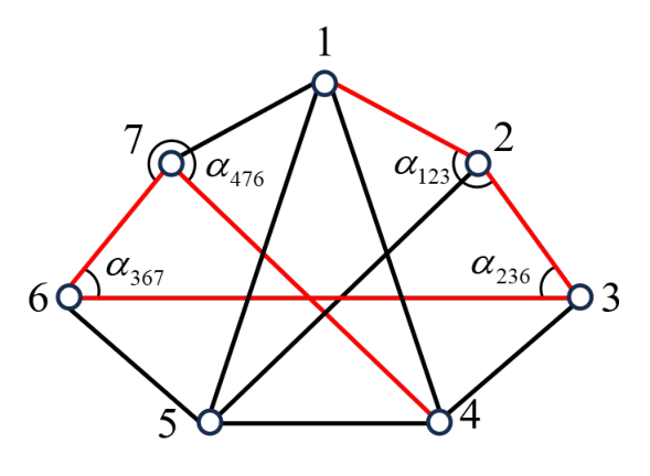
Fig. 5: Based on the common bearing b12b_{12}, any other bearings can be denoted by the product of a rotation matrix determined by the marked signed angles and b21b_{21}. For example, b47b_{47} can be depicted as b47=ℛo​(α47∗)​b12b_{47}=\mathscr{R}_{o}(\alpha^{*}_{47})b_{12} where α47∗=π+α123+α236+α367−α476\alpha^{*}_{47}=\pi+\alpha_{123}+\alpha_{236}+\alpha_{367}-\alpha_{476}.

IV-B Minimal RAISs for Signed Angle Rigidity

The following result provides an intuitive condition to determine RAISs.

Lemma 7

For a framework (𝒢,p)(\mathcal{G},p) in ℝ2\mathbb{R}^{2}, an AIS 𝒯𝒢∗\mathcal{T}^{*}_{\mathcal{G}} is a RAIS if it is angle connected.

Proof:

According to Definition 6, it is sufficient to show rank⁡(RS𝒯𝒢∗​(p))=rank⁡(RS𝒯𝒢​(p))\rank(R^{\mathcal{T}^{*}_{\mathcal{G}}}_{S}(p))=\rank(R^{\mathcal{T}_{\mathcal{G}}}_{S}(p)). Since 𝒯𝒢∗\mathcal{T}^{*}_{\mathcal{G}} is angle connected, for any two edges (i,j),(l,m)∈ℰ(i,j),(l,m)\in\mathcal{E}, one has bl​m=ℛo​(αl​m∗)​bi​jb_{lm}=\mathscr{R}_{o}(\alpha^{*}_{lm})b_{ij} (see Fig. 5 as an example), where

αl​m∗\displaystyle\alpha^{*}_{lm} =\displaystyle\hskip-5.69054pt=\hskip-5.69054pt s​π+∑(i,j,k)∈𝒯𝒢∗ci​j​k​αi​j​k\displaystyle s\pi+\sum_{(i,j,k)\in\mathcal{T}^{*}_{\mathcal{G}}}c_{ijk}\alpha_{ijk} (19)

for some ci​j​k,s∈{±1,0}c_{ijk},s\in\{\pm 1,0\}. Therefore, the signed angle α∈[0,2​π)\alpha\in[0,2\pi) between any pair of bearings in (𝒢,p)(\mathcal{G},p) satisfies

s1​π+α\displaystyle s_{1}\pi+\alpha ={α∗ifsinα∗⩾0,2​π−α∗otherwise,\displaystyle\hskip-5.69054pt=\left\{\begin{array}[]{ll}\alpha^{*}&{\rm if}~\sin\alpha^{*}\geqslant 0,\\ 2\pi-\alpha^{*}&{\rm otherwise},\end{array}\right.

where α∗=s2​π+∑(i,j,k)∈𝒯𝒢∗ci​j​k​αi​j​k\alpha^{*}=s_{2}\pi+\sum_{(i,j,k)\in\mathcal{T}^{*}_{\mathcal{G}}}c_{ijk}\alpha_{ijk} for some s2,ci​j​k∈{0,±1}s_{2},c_{ijk}\in\{0,\pm 1\} and s1∈ℕs_{1}\in\mathbb{N}. Differentiating both sides of (IV-B) w.r.t. time leads to

α˙\displaystyle\dot{\alpha} =\displaystyle\hskip-5.69054pt=\hskip-5.69054pt s3​∑(i,j,k)∈𝒯𝒢∗ci​j​k​α˙i​j​k\displaystyle s_{3}\sum_{(i,j,k)\in\mathcal{T}^{*}_{\mathcal{G}}}c_{ijk}\dot{\alpha}_{ijk} (23)

for some s3∈{±1}s_{3}\in\{\pm 1\}, which means any row in RS𝒯𝒢​(p)R^{\mathcal{T}_{\mathcal{G}}}_{S}(p) can be represented as a linear combination of the rows indexed by 𝒯𝒢∗\mathcal{T}^{*}_{\mathcal{G}}. As a result, rank⁡(RS𝒯𝒢∗​(p))=rank⁡(RS𝒯𝒢​(p))\rank(R^{\mathcal{T}^{*}_{\mathcal{G}}}_{S}(p))=\rank(R^{\mathcal{T}_{\mathcal{G}}}_{S}(p)). ∎

Similar to GAISs, the angle connectivity of RAISs is not necessary, see an example in Fig. 4(a), where 𝒯¯𝒢\bar{\mathcal{T}}_{\mathcal{G}} is a RAIS since rank⁡(RS𝒯¯𝒢​(p))=rank⁡(RS𝒯𝒢​(p))=1<2\rank(R^{\bar{\mathcal{T}}_{\mathcal{G}}}_{S}(p))=\rank(R^{\mathcal{T}_{\mathcal{G}}}_{S}(p))=1<2 but not angle connected. Nonetheless, we can have the following conclusion.

Theorem 8

For an ISAR Laman framework (ℒn,p)(\mathcal{L}_{n},p) in ℝ2\mathbb{R}^{2}, 𝒯ℒn∗⊆𝒯ℒn\mathcal{T}^{*}_{\mathcal{L}_{n}}\subseteq\mathcal{T}_{\mathcal{L}_{n}} is a minimal RAIS if and only if |𝒯¯ℒn|=2​n−4|\bar{\mathcal{T}}_{\mathcal{L}_{n}}|=2n-4 and 𝒯ℒn∗\mathcal{T}^{*}_{\mathcal{L}_{n}} is angle connected.

Proof:

We first note that for an ISAR framework (𝒢,p)(\mathcal{G},p), 𝒯𝒢∗⊆𝒯𝒢\mathcal{T}^{*}_{\mathcal{G}}\subseteq\mathcal{T}_{\mathcal{G}} is a RAIS if and only if rank⁡(RS𝒯𝒢∗​(p))=rank⁡(RS𝒯𝒢​(p))=2​n−4\rank(R^{\mathcal{T}^{*}_{\mathcal{G}}}_{S}(p))=\rank(R^{\mathcal{T}_{\mathcal{G}}}_{S}(p))=2n-4, which implies that |𝒯𝒢∗|≥2​n−4|\mathcal{T}^{*}_{\mathcal{G}}|\geq 2n-4.

The sufficiency follows from Lemma 7 and |𝒯ℒn∗|≥2​n−4|\mathcal{T}^{*}_{\mathcal{L}_{n}}|\geq 2n-4. As for necessity, by employing Lemma 7 and the techniques used in the proof of Theorem 7, it can be verified that the following two cases contradict the fact that 𝒯ℒn∗\mathcal{T}^{*}_{\mathcal{L}_{n}} is minimal to satisfy rank⁡(RS𝒯ℒn∗​(p))=rank⁡(RS𝒯ℒn​(p))\rank(R^{\mathcal{T}^{*}_{\mathcal{L}_{n}}}_{S}(p))=\rank(R^{\mathcal{T}_{\mathcal{L}_{n}}}_{S}(p)): (i) |𝒯ℒn∗|>2​n−4|\mathcal{T}^{*}_{\mathcal{L}_{n}}|>2n-4 and 𝒯ℒn∗\mathcal{T}^{*}_{\mathcal{L}_{n}} is angle connected; (ii) |𝒯ℒn∗|≥2​n−4|\mathcal{T}^{*}_{\mathcal{L}_{n}}|\geq 2n-4 and 𝒯ℒn∗\mathcal{T}^{*}_{\mathcal{L}_{n}} is not angle connected. ∎

Combining Theorem 7 with Theorem 8, we obtain the following corollary, which indicates that the AIS generated by Algorithm 1 is both a minimal GAIS and a minimal RAIS.

Corollary 3

For an ISAR Laman framework (ℒn,p)(\mathcal{L}_{n},p) in ℝ2\mathbb{R}^{2}, the following statements are equivalent:

  • (i)

    𝒯¯ℒn⊆𝒯ℒn\bar{\mathcal{T}}_{\mathcal{L}_{n}}\subseteq\mathcal{T}_{\mathcal{L}_{n}} is a minimal GAIS;

  • (ii)

    𝒯¯ℒn⊆𝒯ℒn\bar{\mathcal{T}}_{\mathcal{L}_{n}}\subseteq\mathcal{T}_{\mathcal{L}_{n}} is a minimal RAIS;

  • (iii)

    |𝒯¯ℒn|=2​n−4|\bar{\mathcal{T}}_{\mathcal{L}_{n}}|=2n-4 and 𝒯¯ℒn\bar{\mathcal{T}}_{\mathcal{L}_{n}} is angle connected.

To demonstrate the results stated above, we summarize the relationship between AISs and signed angle rigidity in Fig. 6.

Refer to caption
Fig. 6: A graph illustrates the relationship between different concepts related to AISs and signed angle rigidity properties. An arrow means ‘implication’. Specifically, ‘A⇒BA\Rightarrow B with a condition noted on the arrow’ means that AA implies BB when the condition holds.

V Signed Angle-Based Sensor Network Localization

In this section, we study the problem of signed angle-based sensor network localization, where each sensor aims to estimate its own location based on signed angle measurements and communications with neighbors. The results established in the previous sections will provide guidance on how to design localizable networks as well as localization algorithms.

V-A Problem Formulation and Network Localizability

Given a sensor network, the sensors can be represented as 𝒱=𝒜​⋃ℱ\mathcal{V}=\mathcal{A}\bigcup\mathcal{F} where the sensors in 𝒜⊆𝒱\mathcal{A}\subseteq\mathcal{V} are called anchors whose locations are known, and the sensors in ℱ=𝒱\𝒜\mathcal{F}=\mathcal{V}\backslash\mathcal{A} are called followers whose locations are to be determined. Furthermore, the real location of the network is denoted by p=(p1,…,pn)⊤p=(p_{1},\dots,p_{n})^{\top}, where pi≠pjp_{i}\neq p_{j} for any pair of sensors i,j∈𝒱i,j\in\mathcal{V}. The interactions between the sensors are indicated by the fixed and undirected sensing graph 𝒢=(𝒱,ℰ)\mathcal{G}=(\mathcal{V},\mathcal{E}).

We use (𝒢,p,𝒜)(\mathcal{G},p,\mathcal{A}) to describe a sensor network and consider the SASNL problem as follows.

Problem 1

Consider a sensor network (𝒢,p,𝒜)(\mathcal{G},p,\mathcal{A}) in ℝ2\mathbb{R}^{2}, design a distributed algorithm for each follower i∈ℱi\in\mathcal{F} to estimate its location pip_{i} merely using the signed angle measurements {αi​j​k}(i,j,k)∈𝒯𝒢\{\alpha_{ijk}\}_{(i,j,k)\in\mathcal{T}_{\mathcal{G}}} and communicated information from neighbors, i.e., seek a solution to the following nonlinear equations,

{p^j−p^k‖p^j−p^k‖=ℛo​(αi​j​k)​p^j−p^i‖p^j−p^i‖∀(i,j,k)∈𝒯𝒢,p^i=pii∈𝒜,\displaystyle\left\{\begin{array}[]{ll}\frac{\hat{p}_{j}-\hat{p}_{k}}{\|\hat{p}_{j}-\hat{p}_{k}\|}=\mathscr{R}_{o}(\alpha_{ijk})\frac{\hat{p}_{j}-\hat{p}_{i}}{\|\hat{p}_{j}-\hat{p}_{i}\|}&\forall(i,j,k)\in\mathcal{T}_{\mathcal{G}},\\ \hat{p}_{i}=p_{i}&i\in\mathcal{A},\end{array}\right.

where p^i\hat{p}_{i} is the estimated location of follower ii.

It should be noted that (1) may have multiple solutions, not all of which correspond to the real location of the network. Therefore, it is necessary to investigate the condition for the existence of a unique solution to (1), which motivates the introduction of the “localizability” notion.

Definition 12

A sensor network (𝒢,p,𝒜)(\mathcal{G},p,\mathcal{A}) in ℝ2\mathbb{R}^{2} is said to be signed angle localizable if the real location pp is the only feasible solution to (1).

The following theorem proposes a necessary and sufficient condition for signed angle localizability.

Theorem 9

For an ISAR framework (𝒢,p)(\mathcal{G},p) in ℝ2\mathbb{R}^{2}, the sensor network (𝒢,p,𝒜)(\mathcal{G},p,\mathcal{A}) is signed angle localizable if and only if |𝒜|≥2|\mathcal{A}|\geq 2.

Proof:

Sufficiency. Let q=(q1⊤,…,qn⊤)⊤∈ℝ2​nq=(q^{\top}_{1},\dots,q^{\top}_{n})^{\top}\in\mathbb{R}^{2n} be a solution to (1). Then, we have q∈ℰ𝒢​(p)q\in\mathscr{E}_{\mathcal{G}}(p). It suffices to show q=pq=p. Since (𝒢,p)(\mathcal{G},p) is ISAR, it follows from Theorem 3 that

q\displaystyle q =\displaystyle\hskip-5.69054pt=\hskip-5.69054pt c⁡(In⊗ℛo​(θ))​p+1n⊗ξ,\displaystyle c(I_{n}\otimes\mathscr{R}_{o}(\theta))p+\textbf{1}_{n}\otimes\xi, (27)

for some c∈ℝ\{0}c\in\mathbb{R}\backslash\{0\}, θ∈[0,2​π)\theta\in[0,2\pi), and ξ∈ℝ2\xi\in\mathbb{R}^{2}. Without loss of generality, let 1,21,2 be the anchors since |𝒜|≥2|\mathcal{A}|\geq 2. It follows from qi=pi,i∈𝒜q_{i}=p_{i},i\in\mathcal{A} that

p1−p2\displaystyle p_{1}-p_{2} =\displaystyle\hskip-5.69054pt=\hskip-5.69054pt q1−q2=c​ℛo​(θ)​(p1−p2),\displaystyle q_{1}-q_{2}=c\mathscr{R}_{o}(\theta)(p_{1}-p_{2}), (28)

which implies c​ℛo​(θ)=I2c\mathscr{R}_{o}(\theta)=I_{2}. Together with the fact that q1=c​ℛo​(θ)​p1+ξ=p1q_{1}=c\mathscr{R}_{o}(\theta)p_{1}+\xi=p_{1}, we have ξ=[0,0]⊤\xi=[0,0]^{\top} and q=pq=p. Hence, (𝒢,p,𝒜)(\mathcal{G},p,\mathcal{A}) is signed-angle-based localizable.

Necessity. It suffices to show that there exists a solution q∈ℝ2​nq\in\mathbb{R}^{2n} of (1) such that q≠pq\neq p when |𝒜|≤1|\mathcal{A}|\leq 1. Without loss of generality, suppose 𝒜={1}\mathcal{A}=\{1\}. Let q=(In⊗ℛo​(π2))​p+𝟏n⊗ηq=(I_{n}\otimes\mathscr{R}_{o}(\frac{\pi}{2}))p+{\bf 1}_{n}\otimes\eta, where η=(I2−ℛo​(π2))​p1\eta=(I_{2}-\mathscr{R}_{o}(\frac{\pi}{2}))p_{1}. It can be verified that q∈ℰ𝒢​(p)q\in\mathscr{E}_{\mathcal{G}}(p), q1=p1q_{1}=p_{1}, and q≠pq\neq p. On the other hand, when 𝒜=∅\mathcal{A}=\varnothing, q=p+1n⊗ξq=p+\textbf{1}_{n}\otimes\xi with any vector ξ∈ℝ2\xi\in\mathbb{R}^{2} is a solution of (1). ∎

We provide examples in Fig. 7 to show non-localizable networks that violate the condition of Theorem 9. Note that the localizability conditions proposed in [18] cannot determine whether the network in Fig. 7(c) is signed angle localizable, as they only apply to trigraphs, which is unnecessary.

Refer to caption
Fig. 7: Examples of sensor networks. Anchors and followers are denoted by solid and hollow dots, respectively. The red arrows represent the infinitesimal signed angle motions corresponding to the followers. (a) and (b) are not signed angle localizable. (c) is signed angle localizable.
Remark 5

Problem 1 involves all signed angles in the sensor network. However, when (𝒢,p)(\mathcal{G},p) is ISAR, only partial signed angles are required. That is, 𝒯𝒢\mathcal{T}_{\mathcal{G}} can be replaced by the minimal GAIS 𝒯¯𝒢\bar{\mathcal{T}}_{\mathcal{G}} induced by Algorithm 1. When the scenario does not support the centralized implementation of Algorithm 1, each sensor i∈𝒱i\in\mathcal{V} can generate a local AIS 𝒯¯𝒢i{{}^{i}}\bar{\mathcal{T}}_{\mathcal{G}} such that the angle index graph (𝒱A​(𝒢i¯),ℰA​(𝒯¯𝒢i))(\mathcal{V}_{A}(\bar{\mathcal{G}_{i}}),\mathcal{E}_{A}({{}^{i}}\bar{\mathcal{T}}_{\mathcal{G}})) is connected and |𝒯¯𝒢i|=|𝒩𝒢i|−1|{{}^{i}}\bar{\mathcal{T}}_{\mathcal{G}}|=|\mathcal{N}^{i}_{\mathcal{G}}|-1, where 𝒢¯i=(𝒱i¯,ℰ¯i)\bar{\mathcal{G}}_{i}=(\bar{\mathcal{V}_{i}},\bar{\mathcal{E}}_{i}), 𝒱i¯=𝒩𝒢i​⋃{i}\bar{\mathcal{V}_{i}}=\mathcal{N}^{i}_{\mathcal{G}}\bigcup\{i\}, and ℰ¯i={(i,j)∈ℰ:j∈𝒩𝒢i}\bar{\mathcal{E}}_{i}=\{(i,j)\in\mathcal{E}:j\in\mathcal{N}^{i}_{\mathcal{G}}\}. Then, the angle index set of the network is 𝒯¯𝒢=⋃i∈𝒱𝒯¯𝒢i\bar{\mathcal{T}}_{\mathcal{G}}=\bigcup_{i\in\mathcal{V}}{{}^{i}}\bar{\mathcal{T}}_{\mathcal{G}} with |𝒯¯𝒢|=∑i∈𝒱(|𝒩𝒢i|−1)=2​|ℰ|−n|\bar{\mathcal{T}}_{\mathcal{G}}|=\sum_{i\in\mathcal{V}}(|\mathcal{N}^{i}_{\mathcal{G}}|-1)=2|\mathcal{E}|-n. It can be verified that 𝒯¯𝒢\bar{\mathcal{T}}_{\mathcal{G}} is angle connected and sufficient for localization according to Lemma 6. However, 𝒯¯𝒢\bar{\mathcal{T}}_{\mathcal{G}} is not minimal even if (𝒢,p)(\mathcal{G},p) is minimally ISAR (i.e., 𝒢\mathcal{G} is a Laman graph) since |𝒯¯𝒢|≥2​(2​n−3)−n=3​n−6>2​n−4|\bar{\mathcal{T}}_{\mathcal{G}}|\geq 2(2n-3)-n=3n-6>2n-4 when n>2n>2.

V-B A Distributed Localization Algorithm

Next, we design a distributed algorithm to achieve the localization objective under the following assumption.

Assumption 1

The sensor network (𝒢,p,𝒜)(\mathcal{G},p,\mathcal{A}) considered satisfies: (i) (𝒢,p)(\mathcal{G},p) is an ISAR Laman framework; (ii) |𝒜|≥2|\mathcal{A}|\geq 2; (iii) there exist two anchors i,j∈𝒜i,j\in\mathcal{A} satisfying (i,j)∈ℰ(i,j)\in\mathcal{E}.

In what follows, we consider that each sensor i∈𝒱i\in\mathcal{V} has access to angle measurements associated with the AIS

𝒯¯𝒢i={(k,i,j)∈𝒱3:(k,i,j)∈𝒯¯𝒢}\displaystyle{{}^{i}}\bar{\mathcal{T}}_{\mathcal{G}}=\{(k,i,j)\in\mathcal{V}^{3}:(k,i,j)\in\bar{\mathcal{T}}_{\mathcal{G}}\} (29)

where 𝒯¯𝒢\bar{\mathcal{T}}_{\mathcal{G}} is induced by Algorithm 1 under Assumption 1.

Inspired by [16], each follower i∈ℱi\in\mathcal{F} generates a random initial value p^i​(0)∈ℝ2\hat{p}_{i}(0)\in\mathbb{R}^{2} and updates its estimated location by

p^˙i​(t)\displaystyle\dot{\hat{p}}_{i}(t) =\displaystyle\hskip-5.69054pt=\hskip-5.69054pt −∑j∈𝒩iP(b^i​j(t))(p^i(t)−p^j(t)),\displaystyle-\sum_{j\in\mathcal{N}_{i}}P(\hat{b}_{ij}(t))(\hat{p}_{i}(t)-\hat{p}_{j}(t)), (30)

where b^i​j​(t)∈ℝ2\hat{b}_{ij}(t)\in\mathbb{R}^{2} is the estimate of the global bearing bi​j≜bi​j​(p)b_{ij}\triangleq b_{ij}(p) and updated through local communications and signed angle measurements and independent of the position estimates p^i​(t)\hat{p}_{i}(t) for all i∈𝒱i\in\mathcal{V} and t≥0t\geq 0, p^j​(t)\hat{p}_{j}(t) is obtained via communications with agent j∈𝒩ij\in\mathcal{N}_{i}. (In the case of anchors, p^i​(t)=pi\hat{p}_{i}(t)=p_{i} for all time t≥0t\geq 0.)

Each sensor i∈𝒱i\in\mathcal{V} generates a random initial estimate b^i​j​(0)∈ℝ2\hat{b}_{ij}(0)\in\mathbb{R}^{2} for each j∈𝒩ij\in\mathcal{N}_{i} and updates b^i​j​(t)\hat{b}_{ij}(t) by

b^˙i​j​(t)\displaystyle\dot{\hat{b}}_{ij}(t) =\displaystyle\hskip-5.69054pt=\hskip-5.69054pt −[∑(j,i,k1)∈𝒯¯𝒢(b^i​j(t)−ℛo⊤(αj​i​k1)b^i​k1(t))\displaystyle-\left[\sum_{(j,i,k_{1})\in\bar{\mathcal{T}}_{\mathcal{G}}}\hskip-5.69054pt(\hat{b}_{ij}(t)-\mathscr{R}^{\top}_{o}(\alpha_{jik_{1}})\hat{b}_{ik_{1}}(t))\right. (31)
+∑(k2,i,j)∈𝒯¯𝒢(b^i​j(t)−ℛo(αk2​i​j)b^i​k2(t))\displaystyle\hskip 14.22636pt+\hskip-7.11317pt\left.\sum_{(k_{2},i,j)\in\bar{\mathcal{T}}_{\mathcal{G}}}\hskip-5.69054pt(\hat{b}_{ij}(t)-\mathscr{R}_{o}(\alpha_{k_{2}ij})\hat{b}_{ik_{2}}(t))\right.
+∑(i,j,k3)∈𝒯¯𝒢(b^i​j(t)+ℛo⊤(αi​j​k3)b^j​k3(t))\displaystyle\hskip 14.22636pt+\hskip-7.11317pt\left.\sum_{(i,j,k_{3})\in\bar{\mathcal{T}}_{\mathcal{G}}}\hskip-5.69054pt(\hat{b}_{ij}(t)+\mathscr{R}^{\top}_{o}(\alpha_{ijk_{3}})\hat{b}_{jk_{3}}(t))\right.
+∑(k4,j,i)∈𝒯¯𝒢(b^i​j(t)+ℛo(αk4​j​i)b^j​k4(t))],\displaystyle\hskip 14.22636pt+\hskip-7.11317pt\left.\sum_{(k_{4},j,i)\in\bar{\mathcal{T}}_{\mathcal{G}}}\hskip-5.69054pt(\hat{b}_{ij}(t)+\mathscr{R}_{o}(\alpha_{k_{4}ji})\hat{b}_{jk_{4}}(t))\right]\hskip-2.84526pt,

where b^j​k3​(t)\hat{b}_{jk_{3}}(t), b^j​k4​(t)\hat{b}_{jk_{4}}(t), αi​j​k3\alpha_{ijk_{3}}, and αk4​j​i\alpha_{k_{4}ji} are obtained via communications with agent j∈𝒩ij\in\mathcal{N}_{i}. (In the case of (i,j)∈ℰ(i,j)\in\mathcal{E} and i,j∈𝒜i,j\in\mathcal{A}, b^i​j​(t)=bi​j\hat{b}_{ij}(t)=b_{ij} and b^˙i​j​(t)=0\dot{\hat{b}}_{ij}(t)=0 for all t≥0t\geq 0, where bi​jb_{ij} is computed from the locations of anchors ii and jj.)

Note that the distributed protocol (30)–(31) is similar to those in [39], but it does not rely on bearing measurements and orientation estimation to get global bearings. Additionally, under the action of (31), b^i​j​(t)\hat{b}_{ij}(t) may not satisfy b^i​j​(t)=b^j​i​(t)\hat{b}_{ij}(t)=\hat{b}_{ji}(t) and ‖b^i​j​(t)‖=1\|\hat{b}_{ij}(t)\|=1 for all t≥0t\geq 0. Hence, P​(b^i​j​(t))P(\hat{b}_{ij}(t)) may not be an orthogonal projection for t≥0t\geq 0. However, these deviations do not affect the convergence of p^i​(t)\hat{p}_{i}(t) to pip_{i} for all i∈ℱi\in\mathcal{F}.

Theorem 10 (Global Convergence)

Under Assumption 1 and the AIS (29), by implementing the algorithm (30)–(31), p^i​(t)\hat{p}_{i}(t) converges to pip_{i} exponentially under arbitrary initial estimates p^i​(0)\hat{p}_{i}(0) and {b^i​j​(0)}j∈𝒩i\{\hat{b}_{ij}(0)\}_{j\in\mathcal{N}_{i}} for all i∈ℱi\in\mathcal{F}.

Proof:

See Appendix VIII-E. ∎

Example 1

Consider a six-sensor network (𝒢,p,𝒜)(\mathcal{G},p,\mathcal{A}), which is described in Fig. 7(c) and satisfies Assumption 1. The initial estimates p^i​(0)\hat{p}_{i}(0) and {b^i​j​(0)}j∈𝒩i\{\hat{b}_{ij}(0)\}_{j\in\mathcal{N}_{i}} are randomly generated for each sensor i∈𝒱i\in\mathcal{V}. By implementing (30)–(31), the convergence trajectories are shown in Fig. 8(a), and the evolutions of bearing and location estimation errors are shown, respectively, in Fig. 8(b). From the simulation results, we observe that the estimated locations converge to real locations asymptotically, which is consistent with Theorem 10.

Fig. 8: (a) Trajectories of the estimation of network locations from randomly initial estates to real positions. (b) Evolution of bearing and location estimation errors.
Remark 6

The first condition in Assumption 1 can be relaxed to ISAR frameworks. When the framework (𝒢,p)(\mathcal{G},p) is ISAR but not a Laman framework, we can first implement Algorithm 1 to induce a minimal GAIS 𝒯¯𝒢\bar{\mathcal{T}}_{\mathcal{G}}. If 𝒯¯𝒢\bar{\mathcal{T}}_{\mathcal{G}} does not contain a triple (i,j,k)(i,j,k) (or (k,j,i)(k,j,i)) satisfying (i,j)∈ℰ(i,j)\in\mathcal{E} and i,j∈𝒜i,j\in\mathcal{A}, we extend 𝒯¯𝒢\bar{\mathcal{T}}_{\mathcal{G}} to include such a triple (i,j,k)(i,j,k) (or (k,j,i)(k,j,i)) for some k∈𝒩jk\in\mathcal{N}_{j} and i,j∈𝒜i,j\in\mathcal{A}. Then, each sensor i∈𝒱i\in\mathcal{V} measures the angles indexed by (29)(\ref{eq:angle measurement set}), and communicates with neighbors j∈𝒩¯ij\in\bar{\mathcal{N}}_{i} to update the estimates b^i​j​(t)\hat{b}_{ij}(t) and p^i​(t)\hat{p}_{i}(t), where 𝒩¯i={j,k∈𝒱:∃(i,j,k),(k,i,j),\bar{\mathcal{N}}_{i}=\{j,k\in\mathcal{V}:\exists(i,j,k),(k,i,j), or (j,k,i)∈𝒯¯𝒢}(j,k,i)\in\bar{\mathcal{T}}_{\mathcal{G}}\}. That is, the subscript “j∈𝒩ij\in\mathcal{N}_{i}” in (30) is replaced by “j∈𝒩¯ij\in\bar{\mathcal{N}}_{i}”. It can be verified that p^i​(t)\hat{p}_{i}(t) globally converges to pip_{i} for all i∈ℱi\in\mathcal{F} under the distributed protocol (30)–(31) when (𝒢,p)(\mathcal{G},p) is ISAR but not a Laman framework.

VI Signed Angle Rigid Formation Control

In this section, we will demonstrate the application of the developed rigidity theory to formation control, where the target formation is described by signed angle constraints and each agent in the formation only measures signed angles to meet these constraints via a distributed control law.

For the group of nn agents moving in the plane, we use 𝒱={1,…,n}\mathcal{V}=\{1,\dots,n\} to label the agents. Let pi≜pi​(t)∈ℝ2p_{i}\triangleq p_{i}(t)\in\mathbb{R}^{2} be the position of agent i∈𝒱i\in\mathcal{V}, βi≜βi​(t)∈[0,2​π)\beta_{i}\triangleq\beta_{i}(t)\in[0,2\pi) be the signed angle from the body frame ∑i\sum_{i} to the coordinate frame ∑g\sum_{g}, p≜[p1⊤,…,pn⊤]p\triangleq[p^{\top}_{1},\dots,p^{\top}_{n}], and β≜[β1,…,βn]\beta\triangleq[\beta_{1},\dots,\beta_{n}]. The position and attitude dynamics of agent ii is

p˙i\displaystyle\dot{p}_{i} =\displaystyle\hskip-5.69054pt=\hskip-5.69054pt ℛo​(βi)​uip​(t),\displaystyle\mathscr{R}_{o}(\beta_{i})u^{p}_{i}(t), (32)
β˙i\displaystyle\dot{\beta}_{i} =\displaystyle\hskip-5.69054pt=\hskip-5.69054pt uia​(t),\displaystyle u^{a}_{i}(t), (33)

where uip​(t)u^{p}_{i}(t) and uia​(t)u^{a}_{i}(t) are the control input to be designed.

The sensing relationship between two neighboring agents is represented as an edge in the undirected graph 𝒢=(𝒱,ℰ)\mathcal{G}=(\mathcal{V},\mathcal{E}). That is, agent ii can measure the signed angle αi​ji∈[0,2​π)\alpha^{i}_{ij}\in[0,2\pi) from the xx-axis to the edge (i,j)(i,j) in the body frame ∑i\sum_{i}, and the signed angles βi​j=βi−βj\beta_{ij}=\beta_{i}-\beta_{j} from ∑i\sum_{i} to ∑j\sum_{j}, if jj is a neighbor of ii in 𝒢\mathcal{G}, see Fig. 9 for illustrations. We adopt a framework (𝒢,p∗)(\mathcal{G},p^{*}) to denote the target formation. The configuration set that has the same shape as the target formation is described as the set ℰ⁡(p∗)\mathscr{E}(p^{*}).

Since ISAR ensures a unique shape of a framework, we consider the following assumption for the target formation.

Assumption 2

The target formation (𝒢,p∗)(\mathcal{G},p^{*}) is ISAR.

Note that ℰ⁡(p∗)\mathscr{E}(p^{*}) is a 4-dimensional smooth manifold under Assumption 2. The signed angle-based formation control problem to be solved is stated as below.

Problem 2

Given a set of signed angle constraints 𝒮={αi​j​k​(p)=αi​j​k​(p∗),(i,j,k)∈𝒯𝒢}\mathcal{S}=\left\{\alpha_{ijk}(p)=\alpha_{ijk}(p^{*}),(i,j,k)\in\mathcal{T}_{\mathcal{G}}\right\} induced by the framework (𝒢,p∗)(\mathcal{G},p^{*}), design a controller for each agent ii based on only the signed angle measurements {αi​ji}j∈𝒩i\left\{\alpha^{i}_{ij}\right\}_{j\in\mathcal{N}_{i}} and {βi​j}j∈𝒩i\{\beta_{ij}\}_{j\in\mathcal{N}_{i}} such that ℰ⁡(p∗)\mathscr{E}(p^{*}) is asymptotically stable.

Under Assumption 2, the graph 𝒢\mathcal{G} must be connected. Therefore, any bearing in the framework (𝒢,p∗)(\mathcal{G},p^{*}) can be represented as the product of a rotation matrix determined by signed angle constraints and a common bearing, see Fig. 5 for an illustration. As a result, the set {αi​j∗}j∈𝒩i\{\alpha^{*}_{ij}\}_{j\in\mathcal{N}_{i}} is available for agent i∈𝒱i\in\mathcal{V}, where αi​j∗\alpha^{*}_{ij} is the signed angle from the common edge (1,2)(1,2) to the edge (i,j)(i,j) in the desired framework (𝒢,p∗)(\mathcal{G},p^{*}), and can be calculated by αi​j∗=s​π+∑(i,j,k)∈𝒯𝒢ci​j​k​αi​j​k∗\alpha^{*}_{ij}=s\pi+\sum_{(i,j,k)\in\mathcal{T_{\mathcal{G}}}}c_{ijk}\alpha^{*}_{ijk} for some s,ci​j​k∈{0,±1}s,c_{ijk}\in\{0,\pm 1\}.

Refer to caption
Fig. 9: The illustration of the measured values required for the controllers.

VI-A The Control Law and Stability Analysis

Inspired by the controllers in [10], we propose the following signed angle-based control law:

uip​(t)\displaystyle u^{p}_{i}(t) =\displaystyle\hskip-5.69054pt=\hskip-5.69054pt −∑j∈𝒩iR¯(αi​ji)η(βi​j,αi​j∗),\displaystyle-\sum_{j\in\mathcal{N}_{i}}\bar{R}(\alpha^{i}_{ij})\eta(\beta_{ij},\alpha^{*}_{ij}), (34)
uia​(t)\displaystyle u^{a}_{i}(t) =\displaystyle\hskip-5.69054pt=\hskip-5.69054pt −∑j∈𝒩iβi​j,\displaystyle-\sum_{j\in\mathcal{N}_{i}}\beta_{ij}, (35)

where η⁡(βi​j,αi​j∗)=ℛo​(2​αi​j∗−βi​j2)​[0,cos⁡βi​j2]⊤\eta(\beta_{ij},\alpha^{*}_{ij})=\mathscr{R}_{o}(\frac{2\alpha^{*}_{ij}-\beta_{ij}}{2})[0,\cos\frac{\beta_{ij}}{2}]^{\top} and

R¯​(αi​ji)=[1−cos⁡2​αi​ji−sin⁡2​αi​ji−sin⁡2​αi​ji1+cos⁡2​αi​ji].\bar{R}(\alpha^{i}_{ij})=\begin{bmatrix}1-\cos 2\alpha^{i}_{ij}&-\sin 2\alpha^{i}_{ij}\\ -\sin 2\alpha^{i}_{ij}&1+\cos 2\alpha^{i}_{ij}\end{bmatrix}.
Theorem 11 (Global Convergence)

Given a group of agents with dynamics (32)–(33) moving in the plane and the target formation (𝒢,p∗)(\mathcal{G},p^{*}) satisfying Assumption 2. By implementing the controller (34)–(35), p⁡(t)p(t) converges to ℰ⁡(p∗)\mathscr{E}(p^{*}) exponentially under arbitrary initial states p⁡(0)p(0) and β⁡(0)\beta(0).

Proof:

Since βi​j\beta_{ij} can be expressed as βi−βj\beta_{i}-\beta_{j}, substituting (35) into (33) leads to

β˙i\displaystyle\dot{\beta}_{i} =\displaystyle\hskip-5.69054pt=\hskip-5.69054pt ∑j∈𝒩i(βj−βi).\displaystyle\sum_{j\in\mathcal{N}_{i}}(\beta_{j}-\beta_{i}). (36)

It can be observed that (36) is the same as the consensus algorithm in [40, Lemma 1.3] under a connected undirected graph 𝒢\mathcal{G}. Therefore, βi​j,(i,j)∈ℰ\beta_{ij},(i,j)\in\mathcal{E} converges to zero exponentially fast for any initial points βi​(0)∈[0,2​π),i∈𝒱\beta_{i}(0)\in[0,2\pi),i\in\mathcal{V}. That is, the body frames of agents will achieve coordinate alignment exponentially. Using similar techniques in the proof of [10, Theorem 15], it can be concluded that the controller (34) will drive bi​j​(p),(i,j)∈ℰb_{ij}(p),(i,j)\in\mathcal{E} to either ℛo​(θ)​bi​j​(p∗)\mathscr{R}_{o}(\theta)b_{ij}(p^{*}) (for almost all initial values) or −ℛo​(θ)​bi​j​(p∗)-\mathscr{R}_{o}(\theta)b_{ij}(p^{*}) (for the remaining case) exponentially fast, where θ∈[0,2​π)\theta\in[0,2\pi). It follows that αi​j​k​(p)→αi​j​k​(p∗),(i,j,k)∈𝒯𝒢\alpha_{ijk}(p)\rightarrow\alpha_{ijk}(p^{*}),(i,j,k)\in\mathcal{T}_{\mathcal{G}} as t→∞t\rightarrow\infty from any initial values. According to Theorem 3, the position p⁡(t)p(t) of the formation converges to the manifold ℰ⁡(p∗)\mathscr{E}(p^{*}) globally. ∎

Theorem 11 implies that the effectiveness of controller (34)–(35) only requires 𝒢\mathcal{G} to contain a Laman subgraph, which is much milder than the graphical conditions in the literature of angle-based formation control [11, 12].

Example 2

Consider a seven-agent formation, whose target formation shape is described in Fig. 5. The initial states {pi​(0)}i∈𝒱\{p_{i}(0)\}_{i\in\mathcal{V}} and βi​(0)i∈𝒱{\beta_{i}(0)}_{i\in\mathcal{V}} are assigned randomly. By implementing the controller (34)–(35), formation trajectories of all agents are shown in Fig. 10(a), and the evolution of signed angles errors is shown in Fig. 10(b). From the simulation results, we observe that the formation achieves the desired shape asymptotically, which is consistent with Theorem 11.

Fig. 10: (a) Trajectories of seven agents from randomly initial positions to final positions. (b) Evolution of signed angles errors.

VII Conclusion

In this paper, signed angle rigidity was reformulated by focusing on graphs. By establishing the complete equivalence between signed angle rigidity and bearing rigidity, we proved that the shape of Laman graphs can be uniquely determined by signed angles for almost all configurations. In order to exclude redundant angle constraints in characterizing signed angle rigidity, an algorithm based on angle index graphs was developed to construct the minimal signed angle constraint set. Building on the developed signed angle rigidity theory, we further designed distributed network localization and formation stabilization algorithms, which are based on signed angle measurements only and achieve global exponential convergence.

However, the developed signed angle rigidity theory is limited to ℝ2\mathbb{R}^{2}. Furthermore, the development of this paper relies on establishing the relationship between signed angle rigidity and bearing rigidity. Similar conclusions may hold for angle rigidity in [11], where the angle constraints contain less information. We leave these theoretical extensions as future research directions.

VIII Appendix: Proofs of Lemmas and Theorems

VIII-A Proof of Lemma 1

Proof: Differentiating both sides of (II-C) w.r.t. time leads to

α˙i​j​k\displaystyle\hskip-5.69054pt\dot{\alpha}_{ijk}\hskip-5.69054pt =\displaystyle= bj​k⊤​Pj​i−sin⁡αi​j​k​‖ej​i‖​p˙i+bj​i⊤​Pj​k−sin⁡αi​j​k​‖ej​k‖​p˙k\displaystyle\hskip-5.69054pt\frac{b_{jk}^{\top}P_{ji}}{-\sin\alpha_{ijk}\|e_{ji}\|}\dot{p}_{i}+\frac{b_{ji}^{\top}P_{jk}}{-\sin\alpha_{ijk}\|e_{jk}\|}\dot{p}_{k} (37)
−(bj​k⊤​Pj​i−sin⁡αi​j​k​‖ej​i‖+bj​i⊤​Pj​k−sin⁡αi​j​k​‖ej​k‖)​p˙j.\displaystyle-\left(\frac{b_{jk}^{\top}P_{ji}}{-\sin\alpha_{ijk}\|e_{ji}\|}+\frac{b_{ji}^{\top}P_{jk}}{-\sin\alpha_{ijk}\|e_{jk}\|}\right)\dot{p}_{j}.

Note that ej​ie_{ji} and ej​ke_{jk} can be described by

ej​i=cj​ix​bj​k+cj​iy​bj​k⊥,ej​k=cj​kx​bj​i+cj​ky​bj​i⊥,\displaystyle e_{ji}=c^{x}_{ji}b_{jk}+c^{y}_{ji}b^{\bot}_{jk},e_{jk}=c^{x}_{jk}b_{ji}+c^{y}_{jk}b^{\bot}_{ji}, (38)

for some cj​ix,cj​iy,cj​kx,cj​ky∈ℝc^{x}_{ji},c^{y}_{ji},c^{x}_{jk},c^{y}_{jk}\in\mathbb{R}. Then, one has

bj​i⊤​Pj​k\displaystyle b^{\top}_{ji}P_{jk}\hskip-5.69054pt =\displaystyle= (cj​ix​bj​k+cj​iy​bj​k⊥)⊤​Pj​k‖ej​i‖=sin⁡αi​j​k​(bj​k)⊤​ℛo​(π2),\displaystyle\hskip-5.69054pt\frac{\left(c^{x}_{ji}b_{jk}+c^{y}_{ji}b^{\bot}_{jk}\right)^{\top}\hskip-5.69054ptP_{jk}}{\|e_{ji}\|}=\sin\alpha_{ijk}(b_{jk})^{\top}\mathscr{R}_{o}(\frac{\pi}{2}),
bj​k⊤​Pj​i\displaystyle b^{\top}_{jk}P_{ji}\hskip-5.69054pt =\displaystyle= (cj​kx​bj​i+cj​ky​bj​i⊥)⊤​Pj​i‖ej​k‖=−sin⁡αi​j​k​(bj​i)⊤​ℛo​(π2).\displaystyle\hskip-5.69054pt\frac{\left(c^{x}_{jk}b_{ji}+c^{y}_{jk}b^{\bot}_{ji}\right)^{\top}\hskip-5.69054ptP_{ji}}{\|e_{jk}\|}=-\sin\alpha_{ijk}(b_{ji})^{\top}\mathscr{R}_{o}(\frac{\pi}{2}).

Together with (37), we have

α˙i​j​k\displaystyle\dot{\alpha}_{ijk}\hskip-5.69054pt =\displaystyle= bj​i⊤​ℛo​(π2)‖ej​i‖​p˙i−bj​k⊤​ℛo​(π2)‖ej​k‖​p˙k\displaystyle\hskip-5.69054pt\frac{b^{\top}_{ji}\mathscr{R}_{o}(\frac{\pi}{2})}{\|e_{ji}\|}\dot{p}_{i}-\frac{b^{\top}_{jk}\mathscr{R}_{o}(\frac{\pi}{2})}{\|e_{jk}\|}\dot{p}_{k} (39)
−(bj​i⊤​ℛo​(π2)‖ej​i‖−bj​k⊤​ℛo​(π2)‖ej​k‖)​p˙j.\displaystyle-\left(\frac{b^{\top}_{ji}\mathscr{R}_{o}(\frac{\pi}{2})}{\|e_{ji}\|}-\frac{b^{\top}_{jk}\mathscr{R}_{o}(\frac{\pi}{2})}{\|e_{jk}\|}\right)\dot{p}_{j}.

It can be observed that (39) does not depend on sin⁡αi​j​k\sin\alpha_{ijk}. Hence, the derivative of (II-C) at αi​j​k∈[0,2​π)\alpha_{ijk}\in[0,2\pi) exists and (8) can be transformed to (9). ∎

VIII-B Proof of Theorem 1

To prove Theorem 1, the following lemma will be used.

Lemma 8

In ℝ2\mathbb{R}^{2}, a framework (𝒢,p)(\mathcal{G},p) is ISAR only if for any vertex j∈𝒱j\in\mathcal{V}, there are at least two distinct neighbors i,k∈𝒩ji,k\in\mathcal{N}_{j} such that |bj​i⊤​bj​k|≠1.|b^{\top}_{ji}b_{jk}|\neq 1.

Proof:

We first show that each vertex has at least two different neighbors. Suppose there is a vertex j∈𝒱j\in\mathcal{V} with only one neighbor i∈𝒱i\in\mathcal{V}. Let q=(0,⋯,0,(bj​i)⊤,0,⋯,0)⊤∈ℝ2​nq=(\textbf{0},\cdots,\textbf{0},(b_{ji})^{\top},\textbf{0},\cdots,\textbf{0})^{\top}\in\mathbb{R}^{2n}, where bj​ib_{ji} consists of the (2​j−1)(2j-1)-th to 2​j2j-th components of qq. According to Lemma 1, for any 𝒯¯𝒢⊆𝒯𝒢\bar{\mathcal{T}}_{\mathcal{G}}\subseteq\mathcal{T}_{\mathcal{G}}, one has

RS𝒯¯𝒢​(p)​q\displaystyle R^{\bar{\mathcal{T}}_{\mathcal{G}}}_{S}(p)q =\displaystyle\hskip-5.69054pt=\hskip-5.69054pt R¯𝒯¯𝒢​(p)​H¯​q=0.\displaystyle\bar{R}_{\bar{\mathcal{T}}_{\mathcal{G}}}(p)\bar{H}q=0. (40)

Therefore, qq is an infinitesimal signed angle motion but not trivial. Hence, a contradiction with the ISAR of (𝒢,p)(\mathcal{G},p) arises.

Similarly, if there is a vertex jj satisfying |𝒩j|≥2|\mathcal{N}_{j}|\geq 2 and |bj​i⊤​bj​k|=1|b^{\top}_{ji}b_{jk}|=1 for any pair of i,k∈𝒩ji,k\in\mathcal{N}_{j}, we can find a non-trivial infinitesimal signed angle motion q=(0,⋯,0,(bj​i)⊤,0,⋯,0)⊤∈ℝ2​nq=(\textbf{0},\cdots,\textbf{0},(b_{ji})^{\top},\textbf{0},\cdots,\textbf{0})^{\top}\in\mathbb{R}^{2n} for some i∈𝒩ji\in\mathcal{N}_{j}, where bj​ib_{ji} consists of the (2​j−1)(2j-1)-th to 2​j2j-th components of qq. ∎

We next prove Theorem 1.

Proof: From the rank condition of ISAR and IBR, it suffices to show that rank⁡(RB​(p))\rank(R_{B}(p)) = 2​n−32n-3 if and only if rank⁡(RS𝒯𝒢​(p))\rank(R^{\mathcal{T}_{\mathcal{G}}}_{S}(p)) = 2​n−42n-4.

According to [11, Theorem 5], we know that for a framework (𝒢,p)(\mathcal{G},p) in ℝ2\mathbb{R}^{2}, rank⁡(RB​(p))=2​n−3\rank(R_{B}(p))=2n-3 if and only if rank⁡(RA𝒯𝒢​(p))=2​n−4\rank(R^{\mathcal{T}_{\mathcal{G}}}_{A}(p))=2n-4, where RA𝒯𝒢​(p)R^{\mathcal{T}_{\mathcal{G}}}_{A}(p) is the rigidity matrix defined in [11] using unsigned angles (i.e., the cosine of the angles) as the entries of the rigidity function11 1 In this paper, we use the triple (i,j,k)(i,j,k) to index the unsigned angle between bj​ib_{ji} and bj​kb_{jk}, which is consistent with the definition in [11].. Therefore, it suffices to show that rank⁡(RA𝒯𝒢​(p))=2​n−4\rank(R^{\mathcal{T}_{\mathcal{G}}}_{A}(p))=2n-4 if and only if rank⁡(RS𝒯𝒢​(p))=2​n−4\rank(R^{\mathcal{T}_{\mathcal{G}}}_{S}(p))=2n-4.

From Lemma 8 and [11], we know that if (𝒢,p)(\mathcal{G},p) satisfies rank⁡(RA𝒯𝒢​(p))=2​n−4\rank(R^{\mathcal{T}_{\mathcal{G}}}_{A}(p))=2n-4 or rank⁡(RS𝒯𝒢​(p))=2​n−4\rank(R^{\mathcal{T}_{\mathcal{G}}}_{S}(p))=2n-4, then for any vertex j∈𝒱j\in\mathcal{V}, there exist at least two distinct neighbors i,k∈𝒩ji,k\in\mathcal{N}_{j} such that |bj​i⊤​bj​k|≠1|b^{\top}_{ji}b_{jk}|\neq 1. As a result, when the framework satisfies rank⁡(RA𝒯𝒢​(p))=2​n−4\rank(R^{\mathcal{T}_{\mathcal{G}}}_{A}(p))=2n-4 or rank⁡(RS𝒯𝒢​(p))=2​n−4\rank(R^{\mathcal{T}_{\mathcal{G}}}_{S}(p))=2n-4, we can find an angle connected set 𝒯𝒢∗⊆𝒯𝒢\mathcal{T}^{*}_{\mathcal{G}}\subseteq\mathcal{T}_{\mathcal{G}} by [11, Algorithm 1], which satisfies sin⁡αi​j​k≠0\sin\alpha_{ijk}\neq 0 for (i,j,k)∈𝒯𝒢∗(i,j,k)\in\mathcal{T}^{*}_{\mathcal{G}} and rank⁡(RA𝒯𝒢∗​(p))=rank⁡(RA𝒯𝒢​(p))\rank(R^{\mathcal{T}^{*}_{\mathcal{G}}}_{A}(p))=\rank(R^{\mathcal{T}_{\mathcal{G}}}_{A}(p)). Moreover, with virtue of Lemma 7 (will be proposed later with its proof independence of this theorem), one has rank⁡(RS𝒯𝒢∗​(p))=rank⁡(RS𝒯𝒢​(p))\rank(R^{\mathcal{T}^{*}_{\mathcal{G}}}_{S}(p))=\rank(R^{\mathcal{T}_{\mathcal{G}}}_{S}(p)).

Necessity. We observe from the angle rigidity matrix in [11] and equation (8) that

RS𝒯𝒢∗​(p)\displaystyle R^{\mathcal{T}^{*}_{\mathcal{G}}}_{S}(p) =\displaystyle\hskip-5.69054pt=\hskip-5.69054pt diag⁡(−1sin​αi​j​k)​RA𝒯𝒢∗​(p),\displaystyle{\rm diag}\left(-\frac{1}{{\rm sin}\alpha_{ijk}}\right)R^{\mathcal{T}^{*}_{\mathcal{G}}}_{A}(p), (41)

where sin​αi​j​k≠0{\rm sin}\alpha_{ijk}\neq 0 for (i,j,k)∈𝒯𝒢∗(i,j,k)\in\mathcal{T}^{*}_{\mathcal{G}}. Since rank⁡(RA𝒯𝒢∗​(p))=rank⁡(RA𝒯𝒢​(p))=2​n−4\rank(R^{\mathcal{T}^{*}_{\mathcal{G}}}_{A}(p))=\rank(R^{\mathcal{T}_{\mathcal{G}}}_{A}(p))=2n-4, one has

rank⁡(RS𝒯𝒢∗​(p))\displaystyle\rank(R^{\mathcal{T}^{*}_{\mathcal{G}}}_{S}(p)) =\displaystyle\hskip-5.69054pt=\hskip-5.69054pt rank⁡(RA𝒯𝒢∗​(p))=2​n−4.\displaystyle\rank(R^{\mathcal{T}^{*}_{\mathcal{G}}}_{A}(p))=2n-4. (42)

Together with the fact that rank⁡(RS𝒯𝒢​(p))=rank⁡(RS𝒯𝒢∗​(p))\rank(R^{\mathcal{T}_{\mathcal{G}}}_{S}(p))=\rank(R^{\mathcal{T}^{*}_{\mathcal{G}}}_{S}(p)), we have rank⁡(RS𝒯𝒢​(p))=2​n−4\rank(R^{\mathcal{T}_{\mathcal{G}}}_{S}(p))=2n-4.

Sufficiency. Similar to the discussion in the proof of necessity, it follows from rank⁡(RS𝒯𝒢∗​(p))=rank⁡(RS𝒯𝒢​(p))=2​n−4\rank(R^{\mathcal{T}^{*}_{\mathcal{G}}}_{S}(p))=\rank(R^{\mathcal{T}_{\mathcal{G}}}_{S}(p))=2n-4 and (41) that rank⁡(RA𝒯𝒢​(p))=2​n−4\rank(R^{\mathcal{T}_{\mathcal{G}}}_{A}(p))=2n-4. ∎

VIII-C Proof of Lemma 3

Proof: Necessity. Note that for a signed angle αi​j​k\alpha_{ijk}, if αi​j​k​(q)=αi​j​k​(p)\alpha_{ijk}(q)=\alpha_{ijk}(p) and bj​i​(q)=ℛo​(θ)​bj​i​(p)b_{ji}(q)=\mathscr{R}_{o}(\theta)b_{ji}(p) for some θ∈[0,2​π)\theta\in[0,2\pi), one has bj​k​(q)=ℛo​(θ)​bj​k​(p)b_{jk}(q)=\mathscr{R}_{o}(\theta)b_{jk}(p). Consider any pair of vertices i,j∈𝒱i,j\in\mathcal{V}, there exists an undirected path 𝒫=(𝒱P,ℰP)\mathcal{P}=(\mathcal{V}_{P},\mathcal{E}_{P}) between ii and jj due to the connectivity of 𝒢\mathcal{G}. It follows from S𝒢​(q)=S𝒢​(p)S_{\mathcal{G}}(q)=S_{\mathcal{G}}(p) that blk−1​lk​(q)=ℛo​(θ)​blk−1​lk​(p)b_{l_{k-1}l_{k}}(q)=\mathscr{R}_{o}(\theta)b_{l_{k-1}l_{k}}(p) for any (lk−1,lk)∈ℰP(l_{k-1},l_{k})\in\mathcal{E}_{P} and some θ∈[0,2​π)\theta\in[0,2\pi). Based on the connectivity of 𝒢\mathcal{G}, we have B𝒢​(q)=(In⊗ℛo​(θ))​B𝒢​(p)B_{\mathcal{G}}(q)=\left(I_{n}\otimes\mathscr{R}_{o}(\theta)\right)B_{\mathcal{G}}(p).

Sufficiency. For any (i,j),(j,k)∈ℰ(i,j),(j,k)\in\mathcal{E}, it follows from B𝒢​(q)=(In⊗ℛo​(θ))​B𝒢​(p)B_{\mathcal{G}}(q)=\left(I_{n}\otimes\mathscr{R}_{o}(\theta)\right)B_{\mathcal{G}}(p) that

bj​k⊤​(q)​bj​i​(q)\displaystyle b^{\top}_{jk}(q)b_{ji}(q)\hskip-5.69054pt =\displaystyle= bj​k⊤​(p)​ℛo⊤​(θ)​ℛo​(θ)​bj​i​(p)\displaystyle\hskip-5.69054ptb^{\top}_{jk}(p)\mathscr{R}^{\top}_{o}(\theta)\mathscr{R}_{o}(\theta)b_{ji}(p) (43)
=\displaystyle= bj​k⊤​(p)​bj​i​(p),\displaystyle\hskip-5.69054ptb^{\top}_{jk}(p)b_{ji}(p),
bj​k⊤​(q)​ℛo​(π2)​bj​i​(q)\displaystyle b^{\top}_{jk}(q)\mathscr{R}_{o}(\frac{\pi}{2})b_{ji}(q)\hskip-5.69054pt =\displaystyle= bj​k⊤​(p)​ℛo⊤​(θ)​ℛo​(π2)​ℛo​(θ)​bj​i​(p)\displaystyle\hskip-5.69054ptb^{\top}_{jk}(p)\mathscr{R}^{\top}_{o}(\theta)\mathscr{R}_{o}(\frac{\pi}{2})\mathscr{R}_{o}(\theta)b_{ji}(p) (44)
=\displaystyle= bj​k⊤​(p)​ℛo​(π2)​bj​i​(p).\displaystyle\hskip-5.69054ptb^{\top}_{jk}(p)\mathscr{R}_{o}(\frac{\pi}{2})b_{ji}(p).

As a result, one has S𝒢​(q)=S𝒢​(p)S_{\mathcal{G}}(q)=S_{\mathcal{G}}(p) according to (II-C)(\ref{eq:signed angle}). ∎

VIII-D Proof of Theorem 3

Proof: (i) ⇔\Leftrightarrow (iii). Suppose (𝒢,p)(\mathcal{G},p) is ISAR. From Lemma 4 and ℰ​(p)⊆ℰ𝒢​(p)\mathscr{E}(p)\subseteq\mathscr{E}_{\mathcal{G}}(p), it suffices to show that for any q∈ℰ𝒢​(p)q\in\mathscr{E}_{\mathcal{G}}(p), it always holds q∈ℰ⁡(p)q\in\mathscr{E}(p). Since 𝒢\mathcal{G} must be connected, it follows from Lemma 3 that q∈ℰ𝒢​(p)q\in\mathscr{E}_{\mathcal{G}}(p) if only if (In⊗ℛo​(θ))−1​q∈B𝒢−1​(B𝒢​(p))(I_{n}\otimes\mathscr{R}_{o}(\theta))^{-1}q\in B^{-1}_{\mathcal{G}}(B_{\mathcal{G}}(p)) for some θ∈[0,2​π)\theta\in[0,2\pi). According to [10, Theorem 6], we know that for a given IBR framework (𝒢,p)(\mathcal{G},p), one has

B−1𝒢(B𝒢(p))={q∈ℝ2​n:q=cp+1n⊗ξ,c∈ℝ\{0},ξ∈ℝ2}.B^{-1}_{\mathcal{G}}(B_{\mathcal{G}}(p))=\{q\in\mathbb{R}^{2n}:q=cp+\textbf{1}_{n}\otimes\xi,c\in\mathbb{R}\backslash\{0\},\\ \xi\in\mathbb{R}^{2}\}. (45)

Since ISAR is equivalent to IBR, then we have

(In⊗ℛo​(θ))−1​q\displaystyle(I_{n}\otimes\mathscr{R}_{o}(\theta))^{-1}q =\displaystyle\hskip-5.69054pt=\hskip-5.69054pt c​p+1n⊗ξ,\displaystyle cp+\textbf{1}_{n}\otimes\xi, (46)

for some c∈ℝ\{0}c\in\mathbb{R}\backslash\{0\} and ξ∈ℝ2\xi\in\mathbb{R}^{2}. As a result, q∈ℰ⁡(p)q\in\mathscr{E}(p).

Suppose the shape of (𝒢,p)(\mathcal{G},p) can be uniquely determined by signed angles up to uniform rotations, translations, and scalings. Then, pp must be non-degenerate, and one has ℰ​(p)=ℰ𝒢​(p)\mathscr{E}(p)=\mathscr{E}_{\mathcal{G}}(p) according to Lemma 4. Therefore, both ℰ⁡(p)\mathscr{E}(p) and ℰ𝒢​(p)\mathscr{E}_{\mathcal{G}}(p) are 4-dimentional smooth manifolds. According to [36, Proposition 3.10], the tangent space of ℰ𝒢​(p)\mathscr{E}_{\mathcal{G}}(p) at pp is 4-dimensional, which indicates that rank⁡(RS𝒯𝒢​(p))=2​n−4\rank(R^{\mathcal{T}_{\mathcal{G}}}_{S}(p))=2n-4. As a result, it follows from Lemma 2 that (𝒢,p)(\mathcal{G},p) is ISAR.

(ii) ⇔\Leftrightarrow (iii). Suppose (𝒢,p)(\mathcal{G},p) is non-degenerate and GSAR. It suffices to show ℰ​(p)=ℰ𝒢​(p)\mathscr{E}(p)=\mathscr{E}_{\mathcal{G}}(p). Since ℰ𝒢​(p)=ℰ𝒦​(p)\mathscr{E}_{\mathcal{G}}(p)=\mathscr{E}_{\mathcal{K}}(p) and (i) ⇔\Leftrightarrow (iii), we just need to show that there exists an ISAR spanning subframework of (𝒦,p)(\mathcal{K},p). From the non-degeneracy of (𝒦,p)(\mathcal{K},p), without loss of generality, we can select three non-collinear vertices from (𝒦,p)(\mathcal{K},p) and index them by 1,2,31,2,3. It can be observed from Lemma 2 that the framework (𝒢′,p′)(\mathcal{G}^{\prime},p^{\prime}) embedded by the triangle 𝒢′\mathcal{G}^{\prime} composed of 1,2,31,2,3 is ISAR, where p′∈ℝ6p^{\prime}\in\mathbb{R}^{6} is the configuration of 1,2,31,2,3 in pp. Since for any 4≤j≤n4\leq j\leq n, there always exist i,k∈{1,2,3}i,k\in\{1,2,3\} such that bj​ib_{ji} and bj​kb_{jk} are not collinear. Combining [11, Theorem 3], Theorem 1, and [17, Lemma 7], we conclude that the framework embedded by the graph constructed by adding vertex jj and edges (j,i)(j,i), (j,k)(j,k) to 𝒢′\mathcal{G}^{\prime} for j=4,⋯nj=4,\cdots n iteratively is ISAR.

Suppose ℰ​(p)=ℰ𝒢​(p)\mathscr{E}(p)=\mathscr{E}_{\mathcal{G}}(p). Then, pp must be non-degenerate, and hence, it suffices to show that for any q∈ℰ𝒢​(p)q\in\mathscr{E}_{\mathcal{G}}(p), it always holds q∈ℰ𝒦​(p)q\in\mathscr{E}_{\mathcal{K}}(p). Since ℰ​(p)=ℰ𝒢​(p)\mathscr{E}(p)=\mathscr{E}_{\mathcal{G}}(p) and q∈ℰ𝒢​(p)q\in\mathscr{E}_{\mathcal{G}}(p), we have

q\displaystyle q =\displaystyle\hskip-5.69054pt=\hskip-5.69054pt c⁡(In⊗ℛo​(θ))​p+1n⊗ξ\displaystyle c(I_{n}\otimes\mathscr{R}_{o}(\theta))p+\textbf{1}_{n}\otimes\xi (47)

for some θ∈[0,2​π),c∈ℝ\{0}\theta\in[0,2\pi),c\in\mathbb{R}\backslash\{0\}, and ξ∈ℝ2\xi\in\mathbb{R}^{2}. Therefore, one has B𝒦​(q)=(In⊗ℛo​(θ))​B𝒦​(p)B_{\mathcal{K}}(q)=\left(I_{n}\otimes\mathscr{R}_{o}(\theta)\right)B_{\mathcal{K}}(p) and S𝒦​(q)=S𝒦​(p)S_{\mathcal{K}}(q)=S_{\mathcal{K}}(p). ∎

VIII-E Proof of Theorem 10

To show convergence, similar to [41, pp. 110], for the network (𝒢,p,𝒜)(\mathcal{G},p,\mathcal{A}) and the AIS 𝒯¯𝒢\bar{\mathcal{T}}_{\mathcal{G}}, we define 𝒢^≜(𝒱^,ℰ^)\hat{\mathcal{G}}\triangleq(\hat{\mathcal{V}},\hat{\mathcal{E}}) as the bearing graph under (31), which is a directed graph describing the pairwise relationship between bearings in the angle errors feedback according to (31). Here vi​j∈𝒱^v_{ij}\in\hat{\mathcal{V}} indexes the estimate b^i​j​(t)\hat{b}_{ij}(t) for i∈𝒱i\in\mathcal{V} and j∈𝒩𝒢ij\in\mathcal{N}^{i}_{\mathcal{G}} and is computed by

vi​j\displaystyle v_{ij} ={2​H​(i,j,|𝒱|)if​i<j,2​H​(i,j,|𝒱|)+1otherwise,\displaystyle=\left\{\begin{array}[]{ll}2H(i,j,|\mathcal{V}|)&{\rm if}~i<j,\\ 2H(i,j,|\mathcal{V}|)+1&{\rm otherwise},\end{array}\right.

a directed edge (vi​k,vi​j)(v_{ik},v_{ij}) from vi​kv_{ik} to vi​jv_{ij} exists in ℰ^\hat{\mathcal{E}} if b^i​k​(t)\hat{b}_{ik}(t) contributes to the update of b^i​j​(t)\hat{b}_{ij}(t), and (vj​k,vi​j)∈ℰ^(v_{jk},v_{ij})\in\hat{\mathcal{E}} if b^j​k​(t)\hat{b}_{jk}(t) is used in the update of b^i​j​(t)\hat{b}_{ij}(t). Let 𝒜¯\bar{\mathcal{A}} be the leader set of the angle index graph (𝒱A​(𝒢),ℰA​(𝒯¯𝒢))(\mathcal{V}_{A}(\mathcal{G}),\mathcal{E}_{A}(\bar{\mathcal{T}}_{\mathcal{G}})), where ai​j∈𝒱A​(𝒢)a_{ij}\in\mathcal{V}_{A}(\mathcal{G}) belongs to 𝒜¯\bar{\mathcal{A}} if i,j∈𝒜i,j\in\mathcal{A}. Let 𝒜^={vi​j,vj​i:ai​j∈𝒜¯}\hat{\mathcal{A}}=\{v_{ij},v_{ji}:a_{ij}\in\bar{\mathcal{A}}\} be the leader set of 𝒢^\hat{\mathcal{G}}. Under Assumption 1, we know that 𝒜^≠∅\hat{\mathcal{A}}\neq\varnothing.

Similarly to the undirected path, given a directed graph 𝒢^\hat{\mathcal{G}}, a directed path from l1∈𝒱^l_{1}\in\hat{\mathcal{V}} to lnP∈𝒱^l_{n_{P}}\in\hat{\mathcal{V}} is a sequence of directed edges of the form (l1,l2)(l_{1},l_{2}),…,(lnP−1,lnP)\dots,(l_{n_{P}-1},l_{n_{P}}).

Next, we provide a useful lemma with regard to 𝒢^\hat{\mathcal{G}}.

Refer to caption
Fig. 11: Illustrations of partial topology relationships of 𝒢^\hat{\mathcal{G}}. (a) There exist (ai​j,ai​k1),(ai​k1,ai​k2)∈ℰA(a_{ij},a_{ik_{1}}),(a_{ik_{1}},a_{ik_{2}})\in\mathcal{E}_{A}. (b) There exist (ai​j,ai​k1),(ai​k1,ak1​j1)∈ℰA(a_{ij},a_{ik_{1}}),(a_{ik_{1}},a_{k_{1}j_{1}})\in\mathcal{E}_{A}. The solid arrow represents the directed edge in 𝒢^\hat{\mathcal{G}} and the dashed arrow represents the existence of a directed path from the starting node to the terminal node.
Lemma 9

Given the network (𝒢,p,𝒜)(\mathcal{G},p,\mathcal{A}) satisfying Assumption 1 and the angle connected AIS 𝒯¯𝒢\bar{\mathcal{T}}_{\mathcal{G}} induced by Algorithm 1, for any pair of elements ai​j,al​k∈𝒱A​(𝒢)\𝒜¯a_{ij},a_{lk}\in\mathcal{V}_{A}(\mathcal{G})\backslash\bar{\mathcal{A}} and the bearing graph 𝒢^\hat{\mathcal{G}} under (31), there exists a directed path from vi​jv_{ij} to vl​kv_{lk} or from vj​iv_{ji} to vl​kv_{lk} in 𝒢^\hat{\mathcal{G}} if there exists an undirected path 𝒫A=(𝒱PA,ℰPA)\mathcal{P}_{A}=(\mathcal{V}^{A}_{P},\mathcal{E}^{A}_{P}) satisfying 𝒱PA​⋂𝒜¯=∅\mathcal{V}^{A}_{P}\bigcap\bar{\mathcal{A}}=\varnothing between ai​ja_{ij} and al​ka_{lk} in the angle index graph 𝒢A​(𝒯¯𝒢)=(𝒱A​(𝒢),ℰA​(𝒯¯𝒢))\mathcal{G}_{A}(\bar{\mathcal{T}}_{\mathcal{G}})=\left(\mathcal{V}_{A}(\mathcal{G}),\mathcal{E}_{A}(\bar{\mathcal{T}}_{\mathcal{G}})\right).

Proof:

For simplicity of notation, denote 𝒢A​(𝒯¯𝒢)=(𝒱A​(𝒢),ℰA​(𝒯¯𝒢))\mathcal{G}_{A}(\bar{\mathcal{T}}_{\mathcal{G}})=\left(\mathcal{V}_{A}(\mathcal{G}),\mathcal{E}_{A}(\bar{\mathcal{T}}_{\mathcal{G}})\right) by 𝒢A=(𝒱A,ℰA)\mathcal{G}_{A}=\left(\mathcal{V}_{A},\mathcal{E}_{A}\right). We first note that for any pair of ai​j,ai​k1∈𝒱A\𝒜¯a_{ij},a_{ik_{1}}\in\mathcal{V}_{A}\backslash\bar{\mathcal{A}} with (ai​j,ai​k1)∈ℰA(a_{ij},a_{ik_{1}})\in\mathcal{E}_{A} , it follows from (31) and the definition of ℰ^\hat{\mathcal{E}} that the directed edges (vi​j,vi​k1)(v_{ij},v_{ik_{1}}), (vi​k1,vi​j)(v_{ik_{1}},v_{ij}), (vi​k1,vj​i)(v_{ik_{1}},v_{ji}), and (vi​j,vk1​i)(v_{ij},v_{k_{1}i}) belong to ℰ^\hat{\mathcal{E}} (see Fig. 11 for examples). It also implies that vi​jv_{ij} and vi​k1v_{ik_{1}} are mutually reachable in 𝒢^\hat{\mathcal{G}} and there are two directed paths from vi​jv_{ij} to vj​iv_{ji} and from vi​k1v_{ik_{1}} to vk1​iv_{k_{1}i}, respectively.

Given any pair of ai​j,al​k∈𝒱A\𝒜¯a_{ij},a_{lk}\in\mathcal{V}_{A}\backslash\bar{\mathcal{A}}. If ai​ja_{ij} is adjacent to al​ka_{lk} in 𝒢A\mathcal{G}_{A}, then the conclusion holds, immediately. If ai​ja_{ij} is not adjacent to al​ka_{lk} in 𝒢A\mathcal{G}_{A}, then there exists an undirected path 𝒫A=(𝒱PA,ℰPA)\mathcal{P}_{A}=(\mathcal{V}^{A}_{P},\mathcal{E}^{A}_{P}) between ai​ja_{ij} and al​ka_{lk}, where 𝒱PA⊆𝒱A\𝒜¯\mathcal{V}^{A}_{P}\subseteq\mathcal{V}_{A}\backslash\bar{\mathcal{A}}, ℰPA⊆ℰA\mathcal{E}^{A}_{P}\subseteq\mathcal{E}_{A}, and |𝒱PA|≥3|\mathcal{V}^{A}_{P}|\geq 3. Without loss of generality, suppose that (ai​j,ai​k1)∈ℰPA(a_{ij},a_{ik_{1}})\in\mathcal{E}^{A}_{P}. The rest of the proof is to show that if ag​ha_{gh} is a neighbor of ai​k1a_{ik_{1}} (other than ai​ja_{ij}) in 𝒫A\mathcal{P}_{A}, there exists two directed paths from vi​jv_{ij} to vg​hv_{gh} and to vh​gv_{hg}, respectively. Then, the statement can be proved by induction.

Since the number of neighbors of ai​k1a_{ik_{1}} in 𝒫A\mathcal{P}_{A} is two, one of the following two cases holds:

Case 1: ∃(ai​k1,ai​k2)∈ℰPA\exists(a_{ik_{1}},a_{ik_{2}})\in\mathcal{E}^{A}_{P}. Since (ai​j,ai​k1),(ai​k1,ai​k2)∈ℰA(a_{ij},a_{ik_{1}}),(a_{ik_{1}},a_{ik_{2}})\in\mathcal{E}_{A}, it follows that for any pair of vertices in {vi​j,vi​k1,vi​k2}\{v_{ij},v_{ik_{1}},v_{ik_{2}}\}, they are mutually reachable in 𝒢^\hat{\mathcal{G}} (see Fig. 11(a)), and there are two directed paths from vi​jv_{ij} to vi​k2v_{ik_{2}} and to vk2​iv_{k_{2}i}, respectively.

Case 2: ∃(ai​k1,ak1​j1)∈ℰPA\exists(a_{ik_{1}},a_{k_{1}j_{1}})\in\mathcal{E}^{A}_{P}. It follows from (ai​j,ai​k1),(ai​k1,ak1​j1)∈ℰA(a_{ij},a_{ik_{1}}),(a_{ik_{1}},a_{k_{1}j_{1}})\in\mathcal{E}_{A} that for any pair of vertices in {vi​k1,vk1​i,vi​j,vk1​j1}\{v_{ik_{1}},v_{k_{1}i},v_{ij},v_{k_{1}j_{1}}\}, they are mutually reachable in 𝒢^\hat{\mathcal{G}} (see Fig. 11(b)), and there are two directed paths from vi​jv_{ij} to vk1​j1v_{k_{1}j_{1}} and to vj1​k1v_{j_{1}k_{1}}, respectively. ∎

To prove Theorem 10, the following lemma will be used.

Lemma 10

Given the network (𝒢,p,𝒜)(\mathcal{G},p,\mathcal{A}) satisfying Assumption 1 and the angle connected AIS 𝒯¯𝒢\bar{\mathcal{T}}_{\mathcal{G}} induced by Algorithm 1, there exists a path from some vertex in 𝒜^\hat{\mathcal{A}} to vl​kv_{lk} for any vertex vl​k∈𝒱^\𝒜^v_{lk}\in\hat{\mathcal{V}}\backslash\hat{\mathcal{A}} under (31).

Proof:

Let the angle index graph of 𝒢\mathcal{G} and 𝒯¯𝒢\bar{\mathcal{T}}_{\mathcal{G}} be 𝒢A=(𝒱A,ℰA)\mathcal{G}_{A}=(\mathcal{V}_{A},\mathcal{E}_{A}). The rest of the proof is to show that under the cases (i) |𝒜¯|=1|\bar{\mathcal{A}}|=1 and (ii) |𝒜¯|≥2|\bar{\mathcal{A}}|\geq 2, the statement holds.

When |𝒜¯|=1|\bar{\mathcal{A}}|=1, without loss of generality, let 𝒜¯={a12}\bar{\mathcal{A}}=\{a_{12}\}, and suppose (a12,a1​k)∈ℰA(a_{12},a_{1k})\in\mathcal{E}_{A}. Since (𝒱A,ℰA)(\mathcal{V}_{A},\mathcal{E}_{A}) is a tree, we consider the following three cases:

Case 1: a12a_{12} is a leaf vertex and ∃(a1​k,a1​k2)∈ℰA\exists(a_{1k},a_{1k_{2}})\in\mathcal{E}_{A}. Since (v12,v1​k)∈ℰ^(v_{12},v_{1k})\in\hat{\mathcal{E}}, it suffices to show that for any vi​j∈𝒱^\𝒜^v_{ij}\in\hat{\mathcal{V}}\backslash\hat{\mathcal{A}}, there exists a directed path from v1​kv_{1k} to vi​jv_{ij}. Recall that a1​k,a1​k2∉𝒜¯a_{1k},a_{1k_{2}}\notin\bar{\mathcal{A}} and the graph 𝒢¯A=(𝒱¯A,ℰ¯A)\bar{\mathcal{G}}_{A}=(\bar{\mathcal{V}}_{A},\bar{\mathcal{E}}_{A}) formed by removing a12a_{12} from 𝒢A\mathcal{G}_{A} is still a connected graph. Hence, there exists an undirected path 𝒫A=(𝒱PA,ℰPA)\mathcal{P}_{A}=(\mathcal{V}^{A}_{P},\mathcal{E}^{A}_{P}) between a1​ka_{1k} and ai​ja_{ij} in the angle index graph 𝒢A\mathcal{G}_{A}, where 𝒱PA⊆𝒱A\𝒜¯\mathcal{V}^{A}_{P}\subseteq\mathcal{V}_{A}\backslash\bar{\mathcal{A}} and ℰPA⊆ℰA\mathcal{E}^{A}_{P}\subseteq\mathcal{E}_{A}. It follows from Lemma 9 that there is a directed path from v1​kv_{1k} to vi​jv_{ij} or from vk​1v_{k1} to vi​jv_{ij} in 𝒢^\hat{\mathcal{G}}. Since (a1​k,a1​k2)∈ℰA(a_{1k},a_{1k_{2}})\in\mathcal{E}_{A} and a1​k,a1​k2∉𝒜¯a_{1k},a_{1k_{2}}\notin\bar{\mathcal{A}}, there is a directed path from v1​kv_{1k} to vk​1v_{k1} and a directed path from v1​kv_{1k} to vi​jv_{ij}.

Case 2: a12a_{12} is a leaf vertex and ∃(a1​k,ak​j1)∈ℰA\exists(a_{1k},a_{kj_{1}})\in\mathcal{E}_{A}. Using techniques similar to Case 1, it can be verified that for any vi​j∈𝒱^\𝒜^v_{ij}\in\hat{\mathcal{V}}\backslash\hat{\mathcal{A}}, there is a directed path from v12v_{12} to vi​jv_{ij}.

Case 3: a12a_{12} is a branch vertex. Let 𝒩a12={a121,…,a12m}\mathcal{N}_{a_{12}}=\{a^{1}_{12},\dots,a^{m}_{12}\} be the neighbor set of a12a_{12} in 𝒢A\mathcal{G}_{A}. Since a12a_{12} is a branch vertex, |𝒩a12|=m≥2|\mathcal{N}_{a_{12}}|=m\geq 2 and we can find mm subtrees 𝒢¯Ai=(𝒱¯Ai,ℰ¯Ai)\bar{\mathcal{G}}^{i}_{A}=\left(\bar{\mathcal{V}}^{i}_{A},\bar{\mathcal{E}}^{i}_{A}\right) (for i=1,…,mi=1,\dots,m) from the tree 𝒢A\mathcal{G}_{A}, where 𝒱¯Ai=𝒱Ai​⋃{a12}\bar{\mathcal{V}}^{i}_{A}=\mathcal{V}^{i}_{A}\bigcup\{a_{12}\}, 𝒱Ai\mathcal{V}^{i}_{A} is the set of the vertices au​v∈𝒱Aa_{uv}\in\mathcal{V}_{A} that have a path from a12a_{12} to au​va_{uv} passing through a12ia^{i}_{12}, and ℰAi={(au​v,ae​f)∈ℰA:au​v,ae​f∈𝒱Ai}\mathcal{E}^{i}_{A}=\{(a_{uv},a_{ef})\in\mathcal{E}_{A}:a_{uv},a_{ef}\in\mathcal{V}^{i}_{A}\}. Note that a12a_{12} is a leaf vertex in each subtree 𝒢Ai\mathcal{G}^{i}_{A}. Therefore, it follows from Case 1–2 that for any aj​k∈𝒱¯Ai\{a12}a_{jk}\in\bar{\mathcal{V}}^{i}_{A}\backslash\{a_{12}\}, there exist two directed paths from v12v_{12} to vj​kv_{jk} and to vk​jv_{kj}, respectively.

When |𝒜¯|≥2|\bar{\mathcal{A}}|\geq 2, one can form the graph 𝒢¯A=(𝒱¯A,ℰ¯A)\bar{\mathcal{G}}_{A}=\left(\bar{\mathcal{V}}_{A},\bar{\mathcal{E}}_{A}\right) by removing the vertices ai​j∈𝒜¯a_{ij}\in\bar{\mathcal{A}} from 𝒢A\mathcal{G}_{A}. Let mm be the number of connected components in 𝒢¯A\bar{\mathcal{G}}_{A}, and denote each connected component by 𝒢¯Ai=(𝒱¯Ai,ℰ¯Ai)\bar{\mathcal{G}}^{i}_{A}=\left(\bar{\mathcal{V}}^{i}_{A},\bar{\mathcal{E}}^{i}_{A}\right) (for i=1,…,mi=1,\dots,m). Since each component 𝒢¯Ai\bar{\mathcal{G}}^{i}_{A} contains a vertex al​k∈𝒱¯Aia_{lk}\in\bar{\mathcal{V}}^{i}_{A} that is adjacent to some vertex au​v∈𝒜¯a_{uv}\in\bar{\mathcal{A}} in 𝒢A\mathcal{G}_{A}, we can further make 𝒱¯Ai=𝒱¯Ai​⋃{au​v}\bar{\mathcal{V}}^{i}_{A}=\bar{\mathcal{V}}^{i}_{A}\bigcup\{a_{uv}\} and ℰ¯Ai=ℰ¯Ai​⋃{(au​v,al​k)}\bar{\mathcal{E}}^{i}_{A}=\bar{\mathcal{E}}^{i}_{A}\bigcup\{(a_{uv},a_{lk})\}. Then 𝒢¯Ai\bar{\mathcal{G}}^{i}_{A} becomes a tree after this augmentation and has only one vertex au​v∈𝒱¯Aia_{uv}\in\bar{\mathcal{V}}^{i}_{A} belonging to 𝒜¯\bar{\mathcal{A}}. The analysis of the case |𝒜¯|=1|\bar{\mathcal{A}}|=1 shows that for any vertex al​k∈𝒱¯Ai\𝒜¯a_{lk}\in\bar{\mathcal{V}}^{i}_{A}\backslash\bar{\mathcal{A}}, there exist two directed path from some vertex in 𝒜^\hat{\mathcal{A}} to vl​kv_{lk} and to vk​lv_{kl}, respectively. ∎

We next prove Theorem 10.

Proof:

Note that according to Theorem 1 and [16, Corollary 3], Assumption 1 implies that (𝒢,p,𝒜)(\mathcal{G},p,\mathcal{A}) is bearing localizable [16]. Therefore, we first prove that b^i​j​(t)\hat{b}_{ij}(t) exponentially converges to the global bearing bi​jb_{ij} for all j∈𝒩ij\in\mathcal{N}_{i}. Then, the proof of the convergence of p^i​(t)\hat{p}_{i}(t) to pip_{i} for all i∈ℱi\in\mathcal{F} is similar to that in [39, Theorem 2].

Let Bi​j≜[bi​j,bi​j⊥]B_{ij}\triangleq[b_{ij},b^{\bot}_{ij}]. Given any αi​j​k∈[0,2​π)\alpha_{ijk}\in[0,2\pi), it follows from ℛo​(αj​i​k)​bi​j=bi​k\mathscr{R}_{o}(\alpha_{jik})b_{ij}=b_{ik} and ℛo​(αj​i​k)​bi​j⊥=bi​k⊥\mathscr{R}_{o}(\alpha_{jik})b^{\bot}_{ij}=b^{\bot}_{ik} that ℛo​(αj​i​k)​Bi​j=Bi​k\mathscr{R}_{o}(\alpha_{jik})B_{ij}=B_{ik}. Therefore, multiplying Bi​j⊤B^{\top}_{ij} on both sides of (31), one has

Bi​j⊤​b^˙i​j\displaystyle B^{\top}_{ij}\dot{\hat{b}}_{ij} =\displaystyle\hskip-5.69054pt=\hskip-5.69054pt −[∑(j,i,k1)∈𝒯¯𝒢(Bi​j⊤b^i​j−Bi​k1⊤b^i​k1)\displaystyle-\left[\sum_{(j,i,k_{1})\in\bar{\mathcal{T}}_{\mathcal{G}}}(B^{\top}_{ij}\hat{b}_{ij}-B^{\top}_{ik_{1}}\hat{b}_{ik_{1}})\right. (51)
+∑(k2,i,j)∈𝒯¯𝒢(Bi​j⊤b^i​j−Bi​k2⊤b^i​k2)\displaystyle\hskip 14.22636pt+\hskip-7.11317pt\left.\sum_{(k_{2},i,j)\in\bar{\mathcal{T}}_{\mathcal{G}}}(B^{\top}_{ij}\hat{b}_{ij}-B^{\top}_{ik_{2}}\hat{b}_{ik_{2}})\right.
+∑(i,j,k3)∈𝒯¯𝒢(Bi​j⊤b^i​j−Bj​k3⊤b^j​k3)\displaystyle\hskip 14.22636pt+\hskip-7.11317pt\left.\sum_{(i,j,k_{3})\in\bar{\mathcal{T}}_{\mathcal{G}}}(B^{\top}_{ij}\hat{b}_{ij}-B^{\top}_{jk_{3}}\hat{b}_{jk_{3}})\right.
+∑(k4,j,i)∈𝒯¯𝒢(Bi​j⊤b^i​j−Bj​k4⊤b^j​k4)],\displaystyle\hskip 14.22636pt+\hskip-7.11317pt\left.\sum_{(k_{4},j,i)\in\bar{\mathcal{T}}_{\mathcal{G}}}(B^{\top}_{ij}\hat{b}_{ij}-B^{\top}_{jk_{4}}\hat{b}_{jk_{4}})\right],

where we use the fact that Bi​j=−Bj​iB_{ij}=-B_{ji}. Let xi​j≜Bi​j⊤​b^i​jx_{ij}\triangleq B^{\top}_{ij}\hat{b}_{ij} for j∈𝒩ij\in\mathcal{N}_{i} and 𝒩vi​j\mathcal{N}_{v_{ij}} be the neighbor set of the vertex vi​jv_{ij} in the bearing graph 𝒢^\hat{\mathcal{G}} under (31). Then, (51) can be rewritten as

x˙i​j\displaystyle\dot{x}_{ij} =\displaystyle\hskip-5.69054pt=\hskip-5.69054pt −[∑vi​k∈𝒩vi​j(xi​j−xi​k)+∑vj​k∈𝒩vi​j(xi​j−xj​k)].\displaystyle-\left[\sum_{v_{ik}\in\mathcal{N}_{v_{ij}}}\hskip-5.69054pt(x_{ij}-x_{ik})+\hskip-5.69054pt\sum_{v_{jk}\in\mathcal{N}_{v_{ij}}}\hskip-5.69054pt(x_{ij}-x_{jk})\right]. (52)

Since for each vertex vi​j∈𝒱^\𝒜^v_{ij}\in\hat{\mathcal{V}}\backslash\hat{\mathcal{A}}, there exists a directed path from some vertex in 𝒜^\hat{\mathcal{A}} to vi​jv_{ij} by Lemma 10, and xj​k=Bj​k⊤​b^j​k=Bj​k⊤​bj​k=[1,0]⊤x_{jk}=B^{\top}_{jk}\hat{b}_{jk}=B^{\top}_{jk}b_{jk}=[1,0]^{\top} for vj​k∈𝒜^v_{jk}\in\hat{\mathcal{A}} and all t≥0t\geq 0, xi​jx_{ij} converges to [1,0]⊤[1,0]^{\top} for all j∈𝒩ij\in\mathcal{N}_{i} according to the result in [40, Theorem 5.1]. It implies that the system converges to

{b^i​j⊤​bi​j=‖b^i​j‖​cos⁡θ=1,b^i​j⊤​bi​j⊥=‖b^i​j‖​sin⁡θ=0,\left\{\begin{array}[]{l}\hat{b}^{\top}_{ij}b_{ij}=\|\hat{b}_{ij}\|\cos\theta=1,\\ \hat{b}^{\top}_{ij}b^{\bot}_{ij}=\|\hat{b}_{ij}\|\sin\theta=0,\end{array}\right. (53)

where θ\theta is the signed angle from b^i​j\hat{b}_{ij} to bi​jb_{ij}. It follows from (53) that ‖b^i​j‖​ℛo​(θ)​[1,0]⊤=[1,0]⊤\|\hat{b}_{ij}\|\mathscr{R}_{o}(\theta)[1,0]^{\top}=[1,0]^{\top}. Therefore, one has ‖b^i​j‖=1\|\hat{b}_{ij}\|=1 and θ=0\theta=0. As a result, b^i​j→bi​j\hat{b}_{ij}\rightarrow b_{ij} as t→∞t\rightarrow\infty for all j∈𝒩ij\in\mathcal{N}_{i}. Since the system (52) is linear, the convergence is exponentially fast [41, Corollary 4.3]. ∎

References

  • [1] James Aspnes, Tolga Eren, David Kiyoshi Goldenberg, A Stephen Morse, Walter Whiteley, Yang Richard Yang, Brian DO Anderson, and Peter N Belhumeur. A theory of network localization. IEEE Transactions on Mobile Computing, 5(12):1663–1678, 2006.
  • [2] J. Fang, M. Cao, A. S. Morse, and B. D. O. Anderson. Sequential localization of sensor networks. SIAM Journal on Control and Optimization, 48(1):321–350, 2009.
  • [3] C. Wan, G. Jing, S. You, and R. Dai. Sensor network localization via alternating rank minimization algorithms. IEEE Transactions on Control of Network Systems, 7(2):1040–1051, 2019.
  • [4] B. D. O. Anderson, C. Yu, B. Fidan, and J. M. Hendrickx. Rigid graph control architectures for autonomous formations. IEEE Control Systems Magazine, 28(6):48–63, 2008.
  • [5] L. Krick, M. E. Broucke, and B. A. Francis. Stabilisation of infinitesimally rigid formations of multi-robot networks. International Journal of control, 82(3):423–439, 2009.
  • [6] Z. Lin, L. Wang, Z. Chen, M. Fu, and Z. Han. Necessary and sufficient graphical conditions for affine formation control. IEEE Transactions on Automatic Control, 61(10):2877–2891, 2015.
  • [7] S. Zhao. Affine formation maneuver control of multiagent systems. IEEE Transactions on Automatic Control, 63(12):4140–4155, 2018.
  • [8] X. Zhang, Q. Yang, F. Xiao, H. Fang, and J. Chen. Linear formation control of multi-agent systems. Automatica, 171:111935, 2025.
  • [9] T. Eren. Formation shape control based on bearing rigidity. International Journal of Control, 85(9):1361–1379, 2012.
  • [10] S. Zhao and D. Zelazo. Bearing rigidity and almost global bearing-only formation stabilization. IEEE Transactions on Automatic Control, 61(5):1255–1268, 2015.
  • [11] G. Jing, G. Zhang, H. W. J. Lee, and L. Wang. Angle-based shape determination theory of planar graphs with application to formation stabilization. Automatica, 105:117–129, 2019.
  • [12] L. Chen, M. Cao, and C. Li. Angle rigidity and its usage to stabilize multiagent formations in 2-D. IEEE Transactions on Automatic Control, 66(8):3667–3681, 2020.
  • [13] K. Cao, Z. Han, X. Li, and L. Xie. Ratio-of-distance rigidity theory with application to similar formation control. IEEE Transactions on Automatic Control, 65(6):2598–2611, 2019.
  • [14] X. Fang, X. Li, and L. Xie. Angle-displacement rigidity theory with application to distributed network localization. IEEE Transactions on Automatic Control, 66(6):2574–2587, 2020.
  • [15] J. Cano and J. Le Ny. Ranging-based localizability optimization for mobile robotic networks. IEEE Transactions on Robotics, 39(4):2842–2860, 2023.
  • [16] S. Zhao and D. Zelazo. Localizability and distributed protocols for bearing-based network localization in arbitrary dimensions. Automatica, 69:334–341, 2016.
  • [17] G. Jing, C. Wan, and R. Dai. Angle-based sensor network localization. IEEE Transactions on Automatic Control, 67(2):840–855, 2021.
  • [18] L. Chen. Triangular angle rigidity for distributed localization in 2D. Automatica, 143:110414, 2022.
  • [19] Y. Wang, S. Liu, and H. Xu. Adaptive formation control of multi-agent systems based on ratio-of-distance rigidity. IEEE Transactions on Automatic Control, 70(3):1988–1995, 2024.
  • [20] K. Cao, M. Cao, and L. Xie. Similar formation control via range and odometry measurements. IEEE Transactions on Cybernetics, 54(6):3765–3776, 2023.
  • [21] K. K. Oh, M. C. Park, and H. S. Ahn. A survey of multi-agent formation control. Automatica, 53:424–440, 2015.
  • [22] L. Asimow and B. Roth. The rigidity of graphs. Transactions of the American Mathematical Society, 245:279–289, 1978.
  • [23] R. Olfati-Saber and R. M. Murray. Graph rigidity and distributed formation stabilization of multi-vehicle systems. In Proceedings of the 41st IEEE Conference on Decision and Control, volume 3, pages 2965–2971, 2002.
  • [24] H. G. De Marina, B. Jayawardhana, and M. Cao. Distributed rotational and translational maneuvering of rigid formations and their applications. IEEE Transactions on Robotics, 32(3):684–697, 2016.
  • [25] J. Chen, B. Jayawardhana, and H. G. De Marina. Distance-based formation-motion control for unicycle agents. In 2023 American Control Conference (ACC), pages 1036–1041, 2023.
  • [26] B. Jackson. Notes on the rigidity of graphs. ADONET-CIRM School on Graphs and Algorithms, Levico Terme, Trento, Italy, Oct. 2007, 31 pages, 2007.
  • [27] M. C. Park, Z. Sun, B. D. O. Anderson, and H. S. Ahn. Distance-based control of 𝒦n\mathcal{K}_{n} formations in general space with almost global convergence. IEEE Transactions on Automatic Control, 63(8):2678–2685, 2017.
  • [28] S. Zhao, Z. Sun, D. Zelazo, M. H. Trinh, and H. S. Ahn. Laman graphs are generically bearing rigid in arbitrary dimensions. In 2017 IEEE 56th Annual Conference on Decision and Control (CDC), pages 3356–3361, 2017.
  • [29] C. Peng and J. Huang. Angle-constrained distributed formation control with disturbance rejection. Automatica, 177:112314, 2025.
  • [30] I. Buckley and M. Egerstedt. Infinitesimal shape-similarity for characterization and control of bearing-only multirobot formations. IEEE Transactions on Robotics, 37(6):1921–1935, 2021.
  • [31] G. Jing, G. Zhang, H. W. Lee, and L. Wang. Weak rigidity theory and its application to formation stabilization. SIAM Journal on Control and Optimization, 56(3):2248–2273, 2018.
  • [32] Y. Zhou. Combinatorial decomposition, generic independence and algebraic complexity of geometric constraints systems: applications in biology and engineering. PhD thesis, University of Florida, 2007.
  • [33] S. Dewar, G. Grasegger, A. Nixon, Z. Rosen, W. Sims, M. Sitharam, and D. Urizar. Angular constraints on planar frameworks. arXiv:2403.16145.
  • [34] B. Hendrickson. Conditions for unique graph realizations. SIAM Journal on Computing, 21(1):65–84, 1992.
  • [35] M. H. Trinh, Q. Van Tran, and H. S. Ahn. Minimal and redundant bearing rigidity: Conditions and applications. IEEE Transactions on Automatic Control, 65(10):4186–4200, 2019.
  • [36] J. M. Lee. Introduction to smooth manifolds. New York, NY, USA: Springer, 2013.
  • [37] T. H. Cormen, C. E. Leiserson, R. L. Rivest, and C. Stein. Introduction to algorithms. MIT press, 2022.
  • [38] G. H. Golub and C. F. Van Loan. Matrix computations. JHU press, 2013.
  • [39] X. Li, X. Luo, and S. Zhao. Globally convergent distributed network localization using locally measured bearings. IEEE Transactions on Control of Network Systems, 7(1):245–253, 2019.
  • [40] W. Ren and Y. Cao. Distributed coordination of multi-agent networks: emergent problems, models, and issues. London, U.K.: Springer-Verlag, 2011.
  • [41] H. K. Khalil. Nonlinear systems, 3rd ed. Englewood Cliffs, NJ, USA: Prentice-Hall, 2002.