Ab initio many-fermion structure calculations on a quantum computer

Introduction.– Ab initio, or first principles, Hamiltonian many-body calculations are widely employed in diverse fields such as quantum chemistry [1, 2], nuclear physics [3, 4, 5, 6], condensed matter physics [7, 8], and quantum field theories [9, 10]. Classical computing faces the daunting challenge of exponentially increasing resources needed to obtain practical results, for example, to test the underlying interactions or search for novel phenomena. Recent advances in quantum computing have unlocked exciting opportunities for performing efficient first-principles many-body calculations [11, 12, 13, 14, 15] but practical algorithms for the full spectra using real-space interactions have yet to emerge. We introduce a general-purpose framework and adopt the self-bound nucleus as an illustrative example to demonstrate how it provides access to the full spectra including determination of the $J$ values with strongly-interacting real-space interactions.

Several quantum algorithms have been adopted to quantum many-body structure calculations, such as the variational quantum eigensolver [13, 14, 16, 17, 18, 19, 20, 21], imaginary time quantum eigensolver [22, 23], and quantum subspace expansion methods [24, 25, 26, 27, 28, 29, 30]. However, these algorithms primarily target the energies of a limited set of states, mostly the ground state, and struggle to access other structural information essential for understanding a system’s response to external probes [31, 32, 33, 34, 35, 36, 37, 38, 39, 40, 41, 42, 43], nuclear reactions [44, 45, 46, 47, 48, 49, 50, 51], and scattering dynamics [52, 53, 54, 55, 56, 57, 58, 59, 60, 61].

Meanwhile, systematically inputting many-fermion Hamiltonians into quantum computers is challenging. Especially, for the Hamiltonians including many-body interactions (e.g., in nuclear and particle physics), the Jordan-Wigner (JW) [62, 63] and Bravyi-Kitaev (BK) [64, 65] schemes become inefficient, as compiling such terms in the Hamiltonian incurs significant overhead and produces extensive Pauli strings. Oracle-based approaches, such as the linear combination of unitaries (LCU) [66, 67], also face growing challenges in designing practical oracles to extract numerous Hamiltonian matrix elements and to uncompute ancilla qubits.

We introduce a new quantum-classical method for ab inito structure calculations of many-fermion systems. This approach incorporates a unique two-fold scan scheme that systematically resolves the eigenenergies and corresponding $J$ values of the Hamiltonian eigenstates. For the first time, we compute the full spectrum, along with the corresponding $J$ values, of ${{}^{20}O}$ using quantum algorithms based on a realistic strong-force interaction [68] developed from fundamental theories [69, 70, 71]. The same method applies directly to relativistic Hamilonians derived from quantum field theory and expressed in the Basis Light-Front Quantization (BLFQ) framework [72, 73, 74, 75, 76, 77].

As a crucial ingredient of this method, we propose a new Hamiltonian input scheme based on a novel circuit representation of the fermion operators that enforces constraints of valid many-body configurations in configuration interaction (CI) calculations. This input scheme eliminates the overhead associated with compiling fermionic operators into Pauli strings that is required by the JW and BK transformations. It is also oracle-free, and there is no need for any uncomputations. Additionally, this input scheme preserves Hamiltonian symmetries, a valuable feature to efficiently pruning Hilbert spaces for tailored eigenvalue calculations.

In the following, we begin with our general discussion of the formalism, Hamiltonian input scheme, and hybrid method. Then, we present the structure calculation of ${{}^{20}}O$ using our method. The proposed method is easily seen to be applicable to CI calculations across various fields.

Formalism.– The Green’s function formalism is a forefront research topic in classical computing [78, 79, 80] as well as quantum computing [81, 82, 83, 84, 85, 86, 87]. We can calculate the retarded Green’s function $G(E)=1/(E-H)$ (referred to as the resolvent), where it is understood that $H$ includes an infinitesimal imaginary part $H\rightarrow H-i\epsilon$ with $\epsilon>0$, and that $||H||_{2}\leq 1$ (one rescales $H$ otherwise). The resolvent can be expressed as [88]:

We approximate $\exp[-iHt]$ with the Chebyshev polynomial (CP) expansion [89, 90]

where $J_{n}(\cdot)$ is the Bessel function of the first kind and $T_{n}(\cdot)$ denotes the CP of the first kind [91].

We evaluate the integral using a discrete Fourier transform [88, 91]. With $N$ grid points, the time is given by $t=\pi\tau$ where $\tau=0,1,\cdots,N-1$. The discrete energy points are $E_{p}=2p/N$, where $p=-N/2,\cdots,N/2$, with $N$ being even. We have

where $\ket{\psi_{\rm in}}$ and $\ket{\psi_{\rm out}}$ are two many-body states. Here, we truncate the CP expansion (i.e., the second summation) utilizing the asymptotic form of $J_{n}(\pi\tau)$ and take $n_{\rm max}(\tau)>e\pi\tau/2\approx 4\tau$ [88]. The truncation error dramatically decreases with increasing $n_{\rm max}(\tau)$ [89, 92]. The Chebyshev moment $\langle\psi_{\rm out}|T_{n}(H)|\psi_{\rm in}\rangle$ captures the many-body nature.

The resolvent has broad applications in solving the structure and dynamics of quantum many-body problems. As a first attempt, we focus on establishing the framework for quantum computing many-fermion structure problems in this work. To date, this has not been discussed in the literature.

Hamiltonian input scheme.– We introduce a novel and efficient input scheme for general second-quantized many-fermion Hamiltonian

Here, for each monomial indexed by $j\in[0,\mathcal{D}-1]$, we denote $Q_{j}\mapsto\{p_{j},q_{j},\cdots,r_{j}\}$ and $P_{j}\mapsto\{u_{j},v_{j},\cdots,w_{j}\}$, where we order the single-particle (SP) bases as $p_{j}<q_{j}<\cdots<r_{j}$ and $u_{j}<v_{j}<\cdots<w_{j}$. The few-body matrix element is $\langle Q_{j}|H|P_{j}\rangle\equiv\langle p_{j},q_{j},\cdots,r_{j}|H|u_{j},v_{j},\cdots,w_{j}\rangle$. We also have $b^{\dagger}_{Q_{j}}\equiv a^{\dagger}_{p_{j}}a^{\dagger}_{q_{j}}\cdots a^{\dagger}_{r_{j}}$ and $b_{P_{j}}\equiv a_{w_{j}}\cdots a_{v_{j}}a_{u_{j}}$. Here the fermion operators act on the occupation mode of SP bases as $a^{\dagger}\ket{0}=\ket{1},\ a\ket{1}=\ket{0},\ a^{\dagger}\ket{1}=a\ket{0}=0$; and they obey the anticommutation relations $\{a_{p},a^{\dagger}_{q}\}=\delta_{p,q},\ \{a_{p},a_{q}\}=\{a^{\dagger}_{p},a^{\dagger}_{q}\}=0$.

This input model is based on the direct basis encoding scheme, which maps $N_{\rm sp}$ SP bases to the qubits in the system register “$s$”. A Fock state is then encoded as $\ket{\mathcal{F}}=\ket{b_{0}}_{0}\ket{b_{1}}_{1}\cdots\ket{b_{N_{\rm sp}-1}}_{N_{\rm sp}-1}$, where each qubit in $s$ corresponds to a specific SP basis, and $\ket{b_{p}}_{p}=\ket{0}$ or $\ket{1}$ denotes that the $p$th basis is vacant or occupied.

We introduce systematic circuit representations for various combinations of fermion operators. These novel representations are reminiscent of Boolean masking [94]. The fermion operators are represented by operations on qubit strings in the system register $s$ that encodes many-fermion states, where corresponding validation information is attached to each processed qubit string to distinguish physical operations from nonphysical ones.

We explain these circuit representations by illustrations in Fig. 1. In addition to the register $s$, we employ two “$error$” registers, $e_{P}$ and $e_{Q}$ (both initialized as $\ket{1}$), to encode the validation information for the actions of annihilation and creation operators, respectively. For example, the circuit for $a_{p}$ operates as follows: (1) controlled by $\ket{b_{p}}_{p}=\ket{1}$, we flip the state $\ket{y}_{e_{P}}=\ket{1}$ to $\ket{0}$; (2) we then apply a $X$ gate to $\ket{b_{p}}_{p}$, aiming to annihilate the occupation; (3) we employ a set of $Z$ gates on qubits with indices ranging from $0$ to $p-1$, whereby these $Z$ gates detect the phase factor due to anticommutation relations. To this end, we note that only a valid operation of $a_{p}$ on $\ket{b_{p}}_{p}$ results in the states $\ket{b_{p}}_{p}=\ket{0}$ and $\ket{y}_{e_{P}}=\ket{0}$.

We apply the same idea to design the circuit for $a^{\dagger}_{q}$, where, in this case, we flip $\ket{y}_{e_{Q}}=\ket{1}$ to $\ket{0}$ controlled by $\ket{b_{q}}_{q}=\ket{0}$. Only a valid operation results in the states $\ket{b_{q}}_{q}=\ket{1}$ and $\ket{y}_{e_{Q}}=\ket{0}$.

With these elementary circuits, we can construct circuit representations of various combinations of fermion operators, as showcased in Fig. 1(c)-(f). Additional optimizations are also applicable, e.g., cancellations of the $Z$ gates and simplifications of paired operators such as $a^{\dagger}_{p}a_{p}$.

Our circuit representations of fermion operators are more intuitive and efficient than the JW and BK transformations, particularly in nuclear and particle physics applications where many-body interactions are present. Unlike the JW and BK transformations, which often require compiling each many-body operator into multiple Pauli strings, our design avoids this compilation overhead; this saving also reduces overhead in subsequent Hamiltonian encoding.

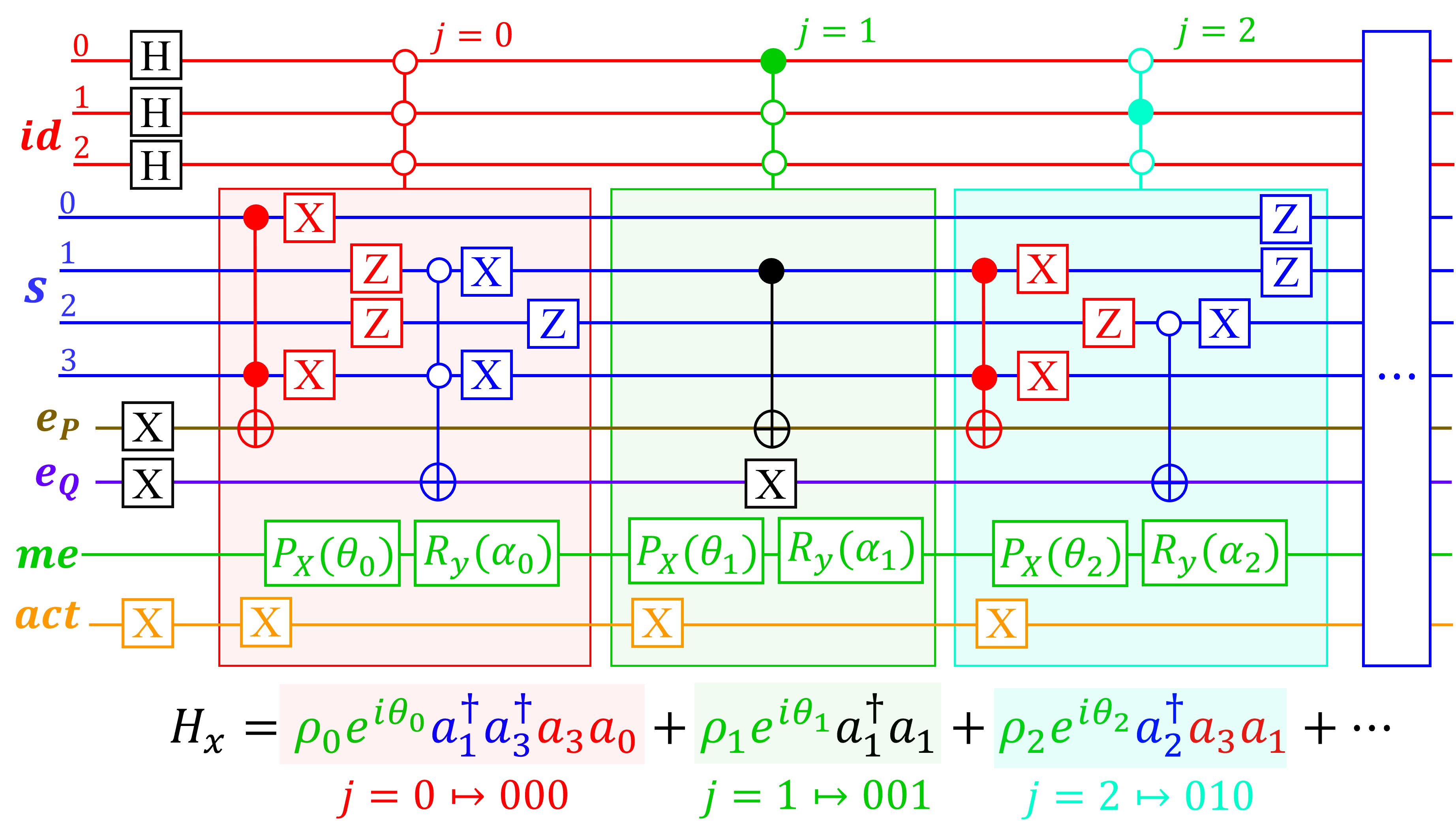
We can block-encode the second-quantized many-fermion Hamiltonian $H$ utilizing the circuit representations of various combinations of fermion operators. By leveraging the concept of Child’s quantum walk [95], we construct the “forward” walk state, the many-fermion state $\ket{\mathcal{F}}$, according to $H$ as

where $\mathscr{T}_{f}$ defines the operation to construct the walk state [see Supplementary Material (SM) for more details] and “$a$” denotes all the ancilla registers. For explanatory purposes, we showcase the circuit for the walk-state construction in Fig. 2.

In Eq. (5), we identify each term in the summation with a specific $j$ value in the “index” register $id$. Indeed, each term tracks the action of the $j$th monomial $\langle Q_{j}|H|P_{j}\rangle b^{\dagger}_{Q_{j}}b_{P_{j}}$ of $H$ on $\ket{\mathcal{F}}$ encoded in the register $s$, where the auxiliary information is recorded by the ancilla registers. $\xi_{\mathcal{F},j}$ records the actions of the $Z$ gates in our fermionic circuit representations and it takes the values of $\pm 1$. As mentioned above, we record the validation messages of sequential actions of $b^{\dagger}_{Q_{j}}$ and $b_{P_{j}}$ on $\ket{\mathcal{F}}$ by the states $\ket{y_{\mathcal{F},j}^{Q}}_{e_{Q}}$ and $\ket{y_{\mathcal{F},j}^{P}}_{e_{P}}$, respectively. While $y_{\mathcal{F},j}^{Q}$ and $y_{\mathcal{F},j}^{P}$ can be either 0 or 1, it is only when $y_{\mathcal{F},j}^{P}=y_{\mathcal{F},j}^{Q}=0$ that $b^{\dagger}_{Q_{j}}b_{P_{j}}\ket{\mathcal{\mathcal{F}}}_{s}$ is valid and produces a physical many-fermion state $\ket{\mathcal{F}_{j}}_{s}$ with the corresponding factor $\xi_{\mathcal{F},j}$.

The matrix-element register “$me$” records the scaled few-body matrix element $\langle Q_{j}|H|P_{j}\rangle/\Xi$ by the state $e^{i\beta_{j}}\ket{\rho_{j}}_{me}$, with $\ket{\rho_{j}}\equiv\rho_{j}\ket{0}+\sqrt{1-\rho^{2}_{j}}\ket{1}$ and the max norm $\Xi\geq\max_{j}|\langle Q_{j}|H|P_{j}\rangle|$. Here the parameters are $\rho_{j}=|\langle Q_{j}|H|P_{j}\rangle|/\Xi\leq 1$ and $\beta_{j}=\arg[\langle Q_{j}|H|P_{j}\rangle]$. In practice, the state $e^{i\beta_{j}}\ket{\rho_{j}}_{me}$ can be prepared by applying the modified phase gate $P_{X}(\beta_{j})$ followed by a $R_{y}(\alpha_{j})$ gate [93] to the register state $\ket{0}_{me}$, with

and $\alpha_{j}=2\arccos\rho_{j}$.

The action register “$act$” is introduced in practical calculations. Since we take $\mathcal{B}\geq\mathcal{D}$ in creating the walk state, $\ket{v_{j}}_{act}$ (initialized as $\ket{1}$) serves to distinguish the null terms in the summation where the index $j$ does not correspond to any monomial in $H$. Those null terms are marked as $v_{j}=1$, while we have $v_{j}=0$ otherwise.

It is straightforward to construct the “backward” walk state with the operation $\mathscr{T}_{b}$ and the many-fermion state $\ket{\mathcal{G}}$ as

These two walk states block-encode the scaled Hamiltonian $H^{\prime}\equiv H/(\mathcal{B}\Xi)$ as (proof available in the SM)

There are at most $O(N^{2k}_{\rm sp})$ monomials in a general many-fermion Hamiltonian that includes up to $k$-body interactions. Our scheme requires $\widetilde{O}(N^{2k+1}_{\rm sp})$ gates to input such a Hamiltonian, which represents the lowest rigorous upper bound on the gate cost for encoding a general $k$-body Hamiltonian. Further incorporation of symmetry principles can reduce this gate cost.

Compared to the conceptual Hamiltonian input scheme based on Child’s quantum walk [96, 95, 97] and other input schemes [77, 98, 99], our scheme provides a practical circuit design, avoiding challenging oracle design, ancilla uncomputation, and quantum-classical communication for accessing Hamiltonian elements.

Compared to standard LCU [66, 67], our scheme eliminates the need for the “Prepare oracle”, which becomes increasingly difficult to design as matrix elements grow. It admits the max norm $\Xi$ for Hamiltonian scaling, which is smaller than the $\mathbb{L}^{1}$ norm in LCU [100], making our approach more time-efficient for Hamiltonian simulations.

Utilizing our many-fermion Hamiltonian input scheme, we can block encode $T_{n}(H^{\prime})$ following the standard protocol of Ref. [101, 102, 103]. The gate cost for encoding $T_{n}(H^{\prime})$ is $\widetilde{O}(n\cdot N^{2k+1}_{\rm sp})$. Specific circuit representations of the CPs are also available in the SM.

Hybrid method.– We introduce a novel quantum-classical algorithm for the structure calculations of many-fermion systems such as those arising in nuclear and hadronic physics. This algorithm is capable of computing the full bound spectrum and the $J$ values of the energy eigenstates.

In particular, for our bound-state applications, we adopt the resolvent to compute the spectral function $F_{\psi}(E_{p})\equiv{\mathfrak{Re}}\langle\psi|G(E_{p})|\psi\rangle$ with the pivot state $\ket{\psi}$. $F_{\psi}(E_{p})$ connects directly to the strength function [88], and its poles correspond to the eigenenergies.

The algorithmic workflow is sketched in Fig. 3(a). We compute the Chebyshev moments $\{\langle\psi|T_{n}(H^{\prime})|\psi\rangle\}$ based on our Hamiltonian input scheme. These moments are input to the classical computer to construct $F_{\psi}(E_{p})$, from which we resolve the spectrum. As our input scheme preserves the symmetry of the Hamiltonian, it enables the so-called “$M$-scheme” calculations. Namely, if we input the pivot to be of a specific projection $M$ of $J$, then only states of $J\geq|M|$ emerge in the resultant spectrum.

This algorithm admits a two-fold scan scheme: the cascading-$M$ scan and the resolution scan. With a sufficient resolution scale (set by the number of grid points $N$), only those energy eigenstates with $J\geq M\geq 1$ appear in the spectrum if we compute using the pivot $\psi_{M}$ of the projection $M$. If additional states emerge when computing $F_{\psi}(E_{p})$ with the pivot $\psi_{M-1}$ of the projection $M-1$, the $J$ value of these emerging states are $J=M-1$. Following this idea, if we compute a set of $F_{\psi}(E_{p})$ based on pivots with projections in the range $M\in[M_{<},M_{>}]$ (with $M_{>}>M_{<}\geq 0$), we can distinguish those eigenstates with $J=M_{>}-1,\cdots,J=M_{<}$.

Finer resolutions may be needed to distinguish closely spaced states. In this case, we improve the resolution by increasing the number of grid points $N$, thereby incorporating more Chebyshev moments. In practical calculations, we can start with a moderate $N$ value for a rough scan. Finer scans with larger $N$ values follow if one wants to resolve even more closely spaced energy eigenstates.

We evaluate the total number of Chebyshev moments required to construct $F_{\psi}(E_{p})$ is $O(\mathcal{B}\Xi/\Delta)$, where $\Delta$ denotes the spectral gap to be resolved between two neighboring states of interest (in, e.g., a low-lying spectrum).

Realistic calculations.– We apply our hybrid method to compute the structure of ${{}^{20}}O$ with a non-relativistic two-body Hamiltonian in a 3D harmonic oscillator (HO) basis. Had we selected a BLFQ example for a hadron, we would employ a 2D HO basis for the transverse motion in light-front coordinates. In this work, we retain the SP bases in the $0d_{5/2}1s_{1/2}$ shell and exclude those in the $0d_{3/2}$ shell. We implement the realistic nuclear interaction from Ref. [68], where we adopt a basis transformation to obtain the few-body Hamiltonian matrix elements in our SP basis set. A total of 110 matrix elements are retained (see Table S3 in the SM). The same techniques can be applied to no-core shell model [105, 106, 6] calculations in future research.

We evaluate the Chebyshev moments using the IBM Qiskit [107] Statevector simulator in noiseless mode; these moments are cross-checked against corresponding classical calculations. In future applications on real quantum hardware, these moments can be evaluated using standard techniques such as the Hadamard test [93].

We apply our two-fold scan scheme to obtain the $J$ values and eigenenergies of the states utilizing simple single-configuration pivots (note that alternative single-configuration pivots may be needed to unconver missing states; additional comments are available in the SM). By applying the cascading-$M$ scan at a coarse resolution scale [Fig. 3(c) and (e)], we can obtain a rough estimation of the eigenenergies and $J$ values of the states that are well-separated from others. With an improved resolution, more spectral information is resolved [Fig. 3(d) and (f)]. In Fig. 3(f), we note regions (marked in cyan and light pink) where finer resolutions are necessary to resolve states with small spectral gaps. Nevertheless, a coarse resolution scale would be sufficient for the low-lying states with larger spectral gaps.

The excitation spectrum of ${{}^{20}}O$ is presented in Fig. 3(b) with the corresponding $J$ values. Our results from the hybrid method agree with the classical results. We expect better agreement with experiments [104] when the SP states of the $0d_{3/2}$ orbit are included.

Summary.– We propose a novel quantum-classical framework for ab initio many-fermion structure calculations. This hybrid method is based on an efficient input scheme for general second-quantized many-fermion Hamiltonians. Using this scheme, we quantum compute the Chebyshev moments and input them into a classical computer to calculate the resolvent, from which we obtain the Hamiltonian spectral function. We introduce a two-fold scan scheme to resolve both the energies and $J$ values of the eigenstates from the spectral function. We apply this hybrid method to compute, for the first time, the structure of ${{}^{20}}O$ based on a realistic strong-interaction Hamiltonian, where we resolve the energies and $J$ values of most eigenstates.

Our approach is directly applicable to hadron spectroscopy [72, 73, 74, 75, 76, 77]. We also envision our framework being applicable to CI calculations in fields such as quantum chemistry [13, 14], condensed matter physics [108, 109], and field theories [110, 111, 74, 75]. Our method easily generalizes to evaluate static and reaction observables using the well-known response theory [79, 80, 32]. Further developments aim to improve circuit designs by utilizing, e.g., quantum machine learning [112, 113], for calculations on NISQ hardware [114].

Acknowledgements.– We acknowledge fruitful discussions with Peter Love, Pieter Maris, and Andrey M. Shirokov. This work was supported in part by US DOE Grant DE-SC0023707 under the Office of Nuclear Physics Quantum Horizons program for the “Nuclei and Hadrons with Quantum computers (NuHaQ)” project. This project was also supported in part by NSF Grant No. 2435255 (NQVL-QSTD: Q-BLUE).

References

- [1] D. Cook, Handbook of Computational Quantum Chemistry, Dover Books on Chemistry (Dover Publications, 2012).
- [2] B. Bauer, S. Bravyi, M. Motta, and G. K.-L. Chan, Quantum algorithms for quantum chemistry and quantum materials science, Chemical Reviews 120, 12685 (2020).
- [3] E. Caurier, G. Martínez-Pinedo, F. Nowacki, A. Poves, and A. P. Zuker, The shell model as a unified view of nuclear structure, Rev. Mod. Phys. 77, 427 (2005).
- [4] J. Carlson, S. Gandolfi, F. Pederiva, S. C. Pieper, R. Schiavilla, K. E. Schmidt, and R. B. Wiringa, Quantum monte carlo methods for nuclear physics, Rev. Mod. Phys. 87, 1067 (2015a).
- [5] M. Hjorth-Jensen, M. P. Lombardo, and U. van Kolck, eds., An Advanced Course in Computational Nuclear Physics, Vol. 936 (Springer, 2017).
- [6] B. R. Barrett, P. Navratil, and J. P. Vary, Ab initio no core shell model, Prog. Part. Nucl. Phys. 69, 131 (2013).
- [7] E. Fradkin, Field Theories of Condensed Matter Physics (Cambridge University Press, 2013).
- [8] M. Schreiber and T. Vojta, Computational Condensed Matter Physics: A Course for Self-Study and the Computer Laboratory, Advanced Texts in Physics (Springer-Verlag GmbH, 2005).
- [9] M. Peskin, An Introduction To Quantum Field Theory (CRC Press, 2018).
- [10] S. J. Brodsky, H.-C. Pauli, and S. S. Pinsky, Quantum chromodynamics and other field theories on the light cone, Physics Reports 301, 299 (1998).
- [11] R. P. Feynman, Simulating physics with computers, International Journal of Theoretical Physics 21 (1982).
- [12] S. Lloyd, Universal quantum simulators, Science 273, 1073 (1996).
- [13] Y. Cao, J. Romero, J. P. Olson, M. Degroote, P. D. Johnson, M. Kieferová, I. D. Kivlichan, T. Menke, B. Peropadre, N. P. D. Sawaya, S. Sim, L. Veis, and A. Aspuru-Guzik, Quantum chemistry in the age of quantum computing, Chemical Reviews 119, 10856–10915 (2019).
- [14] S. McArdle, S. Endo, A. Aspuru-Guzik, S. C. Benjamin, and X. Yuan, Quantum computational chemistry, Reviews of Modern Physics 92, 10.1103/revmodphys.92.015003 (2020).
- [15] T. Albash and D. A. Lidar, Adiabatic quantum computation, Rev. Mod. Phys. 90, 015002 (2018).
- [16] E. F. Dumitrescu, A. J. McCaskey, G. Hagen, G. R. Jansen, T. D. Morris, T. Papenbrock, R. C. Pooser, D. J. Dean, and P. Lougovski, Cloud quantum computing of an atomic nucleus, Phys. Rev. Lett. 120, 210501 (2018).
- [17] J. Tilly, H. Chen, S. Cao, D. Picozzi, K. Setia, Y. Li, E. Grant, L. Wossnig, I. Rungger, G. H. Booth, and J. Tennyson, The variational quantum eigensolver: A review of methods and best practices, Physics Reports 986, 1–128 (2022).
- [18] A. M. Romero, J. Engel, H. L. Tang, and S. E. Economou, Solving nuclear structure problems with the adaptive variational quantum algorithm, Physical Review C 105, 10.1103/physrevc.105.064317 (2022).
- [19] C. Sarma, O. Di Matteo, A. Abhishek, and P. C. Srivastava, Prediction of the neutron drip line in oxygen isotopes using quantum computation, Physical Review C 108, 10.1103/physrevc.108.064305 (2023).
- [20] O. Kiss, M. Grossi, P. Lougovski, F. Sanchez, S. Vallecorsa, and T. Papenbrock, Quantum computing of the nucleus via ordered unitary coupled clusters, Phys. Rev. C 106, 034325 (2022).
- [21] A. Pérez-Obiol, A. M. Romero, J. Menéndez, A. Rios, A. García-Sáez, and B. Juliá-Díaz, Nuclear shell-model simulation in digital quantum computers, Scientific Reports 13, 10.1038/s41598-023-39263-7 (2023).
- [22] M. Motta, C. Sun, A. T. Tan, M. J. O’Rourke, E. Ye, A. J. Minnich, F. G. Brandao, and G. K.-L. Chan, Determining eigenstates and thermal states on a quantum computer using quantum imaginary time evolution, Nature Physics 16, 205 (2020).
- [23] K. Yeter-Aydeniz, R. C. Pooser, and G. Siopsis, Practical quantum computation of chemical and nuclear energy levels using quantum imaginary time evolution and Lanczos algorithms, npj Quantum Inf. 6, 63 (2020), arXiv:1912.06226 [quant-ph] .
- [24] C. L. Cortes and S. K. Gray, Quantum krylov subspace algorithms for ground- and excited-state energy estimation, Physical Review A 105, 10.1103/physreva.105.022417 (2022).
- [25] E. N. Epperly, L. Lin, and Y. Nakatsukasa, A theory of quantum subspace diagonalization, SIAM Journal on Matrix Analysis and Applications 43, 1263–1290 (2022).
- [26] W. Kirby, M. Motta, and A. Mezzacapo, Exact and efficient lanczos method on a quantum computer, Quantum 7, 1018 (2023).
- [27] M. Motta, W. Kirby, I. Liepuoniute, K. J. Sung, J. Cohn, A. Mezzacapo, K. Klymko, N. Nguyen, N. Yoshioka, and J. E. Rice, Subspace methods for electronic structure simulations on quantum computers (2023), arXiv:2312.00178 [quant-ph] .
- [28] N. H. Stair, R. Huang, and F. A. Evangelista, A multireference quantum krylov algorithm for strongly correlated electrons, Journal of Chemical Theory and Computation 16, 2236 (2020), pMID: 32091895, https://doi.org/10.1021/acs.jctc.9b01125 .
- [29] W. Du and J. P. Vary, Systematic input scheme for many-boson Hamiltonians with applications to the two-dimensional 4 theory, Phys. Rev. D 111, 016013 (2025), arXiv:2407.13672 [quant-ph] .
- [30] W. Du and J. P. Vary, Hamiltonian input model and spectroscopy on quantum computers, (2024), arXiv:2402.08969 [quant-ph] .
- [31] J. Carlson and R. Schiavilla, Euclidean proton response in light nuclei, Phys. Rev. Lett. 68, 3682 (1992).
- [32] J. Carlson, S. Gandolfi, F. Pederiva, S. C. Pieper, R. Schiavilla, K. E. Schmidt, and R. B. Wiringa, Quantum Monte Carlo methods for nuclear physics, Rev. Mod. Phys. 87, 1067 (2015b), arXiv:1412.3081 [nucl-th] .
- [33] A. Lovato, S. Gandolfi, J. Carlson, S. C. Pieper, and R. Schiavilla, Electromagnetic and neutral-weak response functions of and , Phys. Rev. C 91, 062501 (2015).
- [34] A. Lovato, S. Gandolfi, J. Carlson, S. C. Pieper, and R. Schiavilla, Electromagnetic response of : A first-principles calculation, Phys. Rev. Lett. 117, 082501 (2016).
- [35] S. Bacca, N. Barnea, G. Hagen, M. Miorelli, G. Orlandini, and T. Papenbrock, Giant and pigmy dipole resonances in , , and from chiral nucleon-nucleon interactions, Phys. Rev. C 90, 064619 (2014).
- [36] J. E. Sobczyk, B. Acharya, S. Bacca, and G. Hagen, Ab initio computation of the longitudinal response function in , Phys. Rev. Lett. 127, 072501 (2021).
- [37] J. E. Sobczyk, B. Acharya, S. Bacca, and G. Hagen, transverse response function from coupled-cluster theory, Phys. Rev. C 109, 025502 (2024a).
- [38] B. Acharya, J. E. Sobczyk, S. Bacca, G. Hagen, and W. Jiang, 16o electroweak response functions from first principles (2024), arXiv:2410.05962 [nucl-th] .
- [39] J. E. Sobczyk, W. Jiang, and A. Roggero, Spin response of neutron matter in ab initio approach (2024b), arXiv:2407.20986 [nucl-th] .
- [40] V. D. Efros, W. Leidemann, and G. Orlandini, Response functions from integral transforms with a lorentz kernel, Physics Letters B 338, 130 (1994).
- [41] A. Roggero and J. Carlson, Dynamic linear response quantum algorithm, Phys. Rev. C 100, 034610 (2019), arXiv:1804.01505 [quant-ph] .
- [42] P. Yin, A. M. Shirokov, H. Li, B. Zhou, X. Zhao, S. Bacca, and J. P. Vary, Alpha-Particle Monopole Form Factors with Ab Initio No-Core Shell Model, (2024), arXiv:2412.18037 [nucl-th] .
- [43] D. M. Kurkcuoglu, A. Roggero, G. N. Perdue, and R. Gupta, Inference of response functions with the help of machine learning algorithms (2025), arXiv:2501.10583 [quant-ph] .
- [44] I. Stetcu, Quantum computing for nuclear reactions, EPJ Web Conf. 322, 03002 (2025).
- [45] R. Weiss, A. Baroni, J. Carlson, and I. Stetcu, Solving reaction dynamics with quantum computing algorithms (2025), arXiv:2404.00202 [quant-ph] .
- [46] V. D. Efros, W. Leidemann, G. Orlandini, and N. Barnea, The lorentz integral transform (lit) method and its applications to perturbation-induced reactions, Journal of Physics G: Nuclear and Particle Physics 34, R459 (2007).
- [47] V. D. Efros, Calculating reactions with use of no-core shell-model states, Phys. Rev. C 99, 034620 (2019).
- [48] M. Goldberger and K. Watson, Collision Theory, Dover books on physics (Dover Publications, 2004).
- [49] M. Hjorth-Jensen, M. Lombardo, and U. van Kolck, An Advanced Course in Computational Nuclear Physics: Bridging the Scales from Quarks to Neutron Stars, Lecture Notes in Physics (Springer International Publishing, 2017).
- [50] S. Baroni, P. Navrátil, and S. Quaglioni, Unified ab initio approach to bound and unbound states: No-core shell model with continuum and its application to 7he, Phys. Rev. C 87, 034326 (2013).
- [51] P. Navrátil, S. Quaglioni, I. Stetcu, and B. R. Barrett, Recent developments in no-core shell-model calculations, Journal of Physics G: Nuclear and Particle Physics 36, 083101 (2009).
- [52] T. Luu, M. J. Savage, A. Schwenk, and J. P. Vary, Nucleon-nucleon scattering in a harmonic potential, Phys. Rev. C 82, 034003 (2010).
- [53] W. Du, P. Yin, Y. Li, G. Chen, W. Zuo, X. Zhao, and J. P. Vary, Coulomb excitation of the deuteron in peripheral collisions with a heavy ion, Phys. Rev. C 97, 064620 (2018), arXiv:1804.01156 [nucl-th] .
- [54] W. Du, J. P. Vary, X. Zhao, and W. Zuo, Quantum simulation of nuclear inelastic scattering, Phys. Rev. A 104, 012611 (2021), arXiv:2006.01369 [nucl-th] .
- [55] S. Sharma, T. Papenbrock, and L. Platter, Scattering phase shifts from a quantum computer, Physical Review C 109, 10.1103/physrevc.109.l061001 (2024).
- [56] P. Wang, W. Du, W. Zuo, and J. P. Vary, Nuclear scattering via quantum computing, Phys. Rev. C 109, 064623 (2024), arXiv:2401.17138 [nucl-th] .
- [57] M. A. Sharaf, A. M. Shirokov, W. Du, and J. P. Vary, Applications of the Modified Hulthén-Kohn Method for Bound and Scattering States, (2024), arXiv:2408.05656 [nucl-th] .
- [58] X. Zhang, Extracting free-space observables from trapped interacting clusters, Phys. Rev. C 101, 051602 (2020), arXiv:1905.05275 [nucl-th] .
- [59] X. Zhang, S. R. Stroberg, P. Navrátil, C. Gwak, J. A. Melendez, R. J. Furnstahl, and J. D. Holt, Ab Initio Calculations of Low-Energy Nuclear Scattering Using Confining Potential Traps, Phys. Rev. Lett. 125, 112503 (2020), arXiv:2004.13575 [nucl-th] .
- [60] X. Zhang, A non-Hermitian quantum mechanics approach for extracting and emulating continuum physics based on bound-state-like calculations, (2024a), arXiv:2408.03309 [nucl-th] .
- [61] X. Zhang, A non-Hermitian quantum mechanics approach for extracting and emulating continuum physics based on bound-state-like calculations: technical details, (2024b), arXiv:2411.06712 [nucl-th] .
- [62] P. Jordan and E. Wigner, über das paulische äquivalenzverbot, Z. Physik 47 (1928).
- [63] M. A. Nielsen, The fermionic canonical commutation relations and the jordan-wigner transform (2005).
- [64] S. B. Bravyi and A. Y. Kitaev, Fermionic quantum computation, Annals of Physics 298, 210–226 (2002).
- [65] J. T. Seeley, M. J. Richard, and P. J. Love, The bravyi-kitaev transformation for quantum computation of electronic structure, The Journal of Chemical Physics 137, 10.1063/1.4768229 (2012).
- [66] A. M. Childs and N. Wiebe, Hamiltonian simulation using linear combinations of unitary operations, Quantum Inf. Comput. 12, 901 (2012).
- [67] D. W. Berry, A. M. Childs, R. Cleve, R. Kothari, and R. D. Somma, Simulating hamiltonian dynamics with a truncated taylor series, Phys. Rev. Lett. 114, 090502 (2015).
- [68] I. J. Shin, N. A. Smirnova, A. M. Shirokov, Z. Yang, B. R. Barrett, Z. Li, Y. Kim, P. Maris, and J. P. Vary, Improving the sd-shell effective interaction obtained from the Daejeon16 nucleon-nucleon interaction, Phys. Rev. C 110, 034306 (2024).
- [69] E. Epelbaum, H.-W. Hammer, and U.-G. Meissner, Modern Theory of Nuclear Forces, Rev. Mod. Phys. 81, 1773 (2009), arXiv:0811.1338 [nucl-th] .
- [70] E. Epelbaum, H. Krebs, and U. G. Meißner, Improved chiral nucleon-nucleon potential up to next-to-next-to-next-to-leading order, Eur. Phys. J. A 51, 53 (2015a), arXiv:1412.0142 [nucl-th] .
- [71] E. Epelbaum, H. Krebs, and U. G. Meißner, Precision nucleon-nucleon potential at fifth order in the chiral expansion, Phys. Rev. Lett. 115, 122301 (2015b), arXiv:1412.4623 [nucl-th] .
- [72] J. P. Vary, H. Honkanen, J. Li, P. Maris, S. J. Brodsky, A. Harindranath, G. F. de Teramond, P. Sternberg, E. G. Ng, and C. Yang, Hamiltonian light-front field theory in a basis function approach, Phys. Rev. C 81, 035205 (2010), arXiv:0905.1411 [nucl-th] .
- [73] W. Qian, S. Jia, Y. Li, and J. P. Vary, Light mesons within the basis light-front quantization framework, Phys. Rev. C 102, 055207 (2020), arXiv:2005.13806 [nucl-th] .
- [74] M. Kreshchuk, W. M. Kirby, G. Goldstein, H. Beauchemin, and P. J. Love, Quantum simulation of quantum field theory in the light-front formulation, Phys. Rev. A 105, 032418 (2022), arXiv:2002.04016 [quant-ph] .
- [75] M. Kreshchuk, S. Jia, W. M. Kirby, G. Goldstein, J. P. Vary, and P. J. Love, Simulating Hadronic Physics on NISQ devices using Basis Light-Front Quantization, Phys. Rev. A 103, 062601 (2021), arXiv:2011.13443 [quant-ph] .
- [76] W. Du, Y. Li, X. Zhao, G. A. Miller, and J. P. Vary, Basis Light-Front Quantization for a Chiral Nucleon-Pion Lagrangian, Phys. Rev. C 101, 035202 (2020), arXiv:1911.10762 [nucl-th] .
- [77] W. Du and J. P. Vary, Multinucleon structure and dynamics via quantum computing, Phys. Rev. A 108, 052614 (2023), arXiv:2304.04838 [nucl-th] .
- [78] J. Schirmer, Many-Body Methods for Atoms, Molecules and Clusters, Lecture Notes in Chemistry (Springer International Publishing, 2018).
- [79] G. Stefanucci and R. van Leeuwen, Nonequilibrium Many-Body Theory of Quantum Systems: A Modern Introduction (Cambridge University Press, 2025).
- [80] A. Fetter and J. Walecka, Quantum Theory of Many-particle Systems, Dover Books on Physics (Dover Publications, 2003).
- [81] E. Kökcü, H. A. Labib, J. K. Freericks, and A. F. Kemper, A linear response framework for quantum simulation of bosonic and fermionic correlation functions, Nature Commun. 15, 3881 (2024), arXiv:2302.10219 [quant-ph] .
- [82] P. W. K. Jensen, P. D. Johnson, and A. A. Kunitsa, Near-term quantum algorithm for computing molecular and materials properties based on recursive variational series methods, Physical Review A 108, 10.1103/physreva.108.022422 (2023a).
- [83] Y. Tong, D. An, N. Wiebe, and L. Lin, Fast inversion, preconditioned quantum linear system solvers, fast green’s-function computation, and fast evaluation of matrix functions, Phys. Rev. A 104, 032422 (2021).
- [84] T. Keen, E. Dumitrescu, and Y. Wang, Quantum algorithms for ground-state preparation and green’s function calculation (2021), arXiv:2112.05731 [quant-ph] .
- [85] F. Libbi, J. Rizzo, F. Tacchino, N. Marzari, and I. Tavernelli, Effective calculation of the green’s function in the time domain on near-term quantum processors, Phys. Rev. Res. 4, 043038 (2022).
- [86] R. Sakurai, W. Mizukami, and H. Shinaoka, Hybrid quantum-classical algorithm for computing imaginary-time correlation functions, Phys. Rev. Res. 4, 023219 (2022).
- [87] S. Endo, I. Kurata, and Y. O. Nakagawa, Calculation of the green’s function on near-term quantum computers, Phys. Rev. Res. 2, 033281 (2020).
- [88] A. Volya, Time-dependent approach to the continuum shell model, Phys. Rev. C 79, 044308 (2009).
- [89] H. Tal‐Ezer and R. Kosloff, An accurate and efficient scheme for propagating the time dependent schrödinger equation, The Journal of Chemical Physics 81, 3967 (1984), https://pubs.aip.org/aip/jcp/article-pdf/81/9/3967/18950222/3967_1_online.pdf .
- [90] A. Weiße, G. Wellein, A. Alvermann, and H. Fehske, The kernel polynomial method, Rev. Mod. Phys. 78, 275 (2006).
- [91] G. Arfken, G. Arfken, H. Weber, and F. Harris, Mathematical Methods for Physicists: A Comprehensive Guide (Elsevier Science, 2013).
- [92] P. W. K. Jensen, P. D. Johnson, and A. A. Kunitsa, Near-term quantum algorithm for computing molecular and materials properties based on recursive variational series methods, Phys. Rev. A 108, 022422 (2023b).
- [93] M. Nielsen and I. Chuang, Quantum Computation and Quantum Information: 10th Anniversary Edition (Cambridge University Press, 2010).
- [94] T. Helgaker, P. Jorgensen, and J. Olsen, Molecular Electronic-Structure Theory (Wiley, 2014).
- [95] A. M. Childs, On the relationship between continuous- and discrete-time quantum walk, Communications in Mathematical Physics 294, 581–603 (2009a).
- [96] A. M. Childs, Universal computation by quantum walk, Phys. Rev. Lett. 102, 180501 (2009b).
- [97] D. W. Berry and A. M. Childs, Black-box hamiltonian simulation and unitary implementation, Quantum Information and Computation 12, 29 (2012).
- [98] D. Liu, W. Du, L. Lin, J. P. Vary, and C. Yang, An Efficient Quantum Circuit for Block Encoding a Pairing Hamiltonian, (2024), arXiv:2402.11205 [nucl-th] .
- [99] W. A. Simon, C. M. Gustin, K. Serafin, A. Ralli, G. R. Goldstein, and P. J. Love, Ladder operator block-encoding (2025), arXiv:2503.11641 [quant-ph] .
- [100] R. Babbush, D. W. Berry, I. D. Kivlichan, A. Y. Wei, P. J. Love, and A. Aspuru-Guzik, Exponentially more precise quantum simulation of fermions in second quantization, New Journal of Physics 18, 033032 (2016).
- [101] G. H. Low and I. L. Chuang, Optimal hamiltonian simulation by quantum signal processing, Phys. Rev. Lett. 118, 010501 (2017).
- [102] A. Gilyén, Y. Su, G. H. Low, and N. Wiebe, Quantum singular value transformation and beyond: exponential improvements for quantum matrix arithmetics, in Proceedings of the 51st Annual ACM SIGACT Symposium on Theory of Computing (2019) pp. 193–204.
- [103] L. Lin, Lecture notes on quantum algorithms for scientific computation (2022), arXiv:2201.08309 [quant-ph] .
- [104] National nuclear data center, http://www.nndc.bnl.gov/ensarchivals/, accessed on 2024-01-23.
- [105] P. Navratil, J. P. Vary, and B. R. Barrett, Properties of C-12 in the ab initio nuclear shell model, Phys. Rev. Lett. 84, 5728 (2000a), arXiv:nucl-th/0004058 .
- [106] P. Navratil, J. P. Vary, and B. R. Barrett, Large basis ab initio no-core shell model and its application to C-12, Phys. Rev. C 62, 054311 (2000b).
- [107] Qiskit contributors, Qiskit: An open-source framework for quantum computing (2023).
- [108] N. Yoshioka, T. Okubo, Y. Suzuki, Y. Koizumi, and W. Mizukami, Hunting for quantum-classical crossover in condensed matter problems, npj Quantum Inf. 10, 45 (2024), arXiv:2210.14109 [quant-ph] .
- [109] Y.-X. Yao, N. Gomes, F. Zhang, C.-Z. Wang, K.-M. Ho, T. Iadecola, and P. P. Orth, Adaptive variational quantum dynamics simulations, PRX Quantum 2, 030307 (2021).
- [110] C. W. Bauer, Z. Davoudi, N. Klco, and M. J. Savage, Quantum simulation of fundamental particles and forces, Nature Rev. Phys. 5, 420 (2023a), arXiv:2404.06298 [hep-ph] .
- [111] C. W. Bauer, Z. Davoudi, A. B. Balantekin, T. Bhattacharya, M. Carena, W. A. de Jong, P. Draper, A. El-Khadra, N. Gemelke, M. Hanada, D. Kharzeev, H. Lamm, Y.-Y. Li, J. Liu, M. Lukin, Y. Meurice, C. Monroe, B. Nachman, G. Pagano, J. Preskill, E. Rinaldi, A. Roggero, D. I. Santiago, M. J. Savage, I. Siddiqi, G. Siopsis, D. Van Zanten, N. Wiebe, Y. Yamauchi, K. Yeter-Aydeniz, and S. Zorzetti, Quantum simulation for high-energy physics, PRX Quantum 4, 027001 (2023b).
- [112] J. Biamonte, P. Wittek, N. Pancotti, P. Rebentrost, N. Wiebe, and S. Lloyd, Quantum machine learning, Nature 549, 195–202 (2017).
- [113] Y. Wang and J. Liu, A comprehensive review of quantum machine learning: from nisq to fault tolerance, Reports on Progress in Physics 87, 116402 (2024).
- [114] J. Preskill, Quantum Computing in the NISQ era and beyond, Quantum 2, 79 (2018).
- [115] J. Suhonen, From Nucleons to Nucleus: Concepts of Microscopic Nuclear Theory, Theoretical and Mathematical Physics (Springer Berlin Heidelberg, 2007).
Supplementary Material: