Depth-Guided Bundle Sampling for Efficient Generalizable Neural Radiance Field ReconstructionThanks: This work is supported by National Key R&D Program of China under Grant No. 2021YFF0900701, and the National Natural Science Foundation of China under Grant No. 62001432.

Li Fang Affiliation: Key Laboratory of Media Audio and Video (Communication University of China)Ministry of Education, Beijing 100024, China Email: lifang8902@cuc.edu.cn Hao Zhu Affiliation: School of Electronic Science and Engineering, Nanjing University, Nanjing 210023, China Email: chenll@cuc.edu.cn Longlong Chen Affiliation: Key Laboratory of Media Audio and Video (Communication University of China)Ministry of Education, Beijing 100024, China Email: hufei@cuc.edu.cn Fei Hu ^†^†thanks: Corresponding author. Affiliation: Key Laboratory of Media Audio and Video (Communication University of China)Ministry of Education, Beijing 100024, China Email: yelong@cuc.edu.cn Long Ye Affiliation: Key Laboratory of Media Audio and Video (Communication University of China)Ministry of Education, Beijing 100024, China Email: zhuhaophoto@nju.edu.cn Zhan Ma Affiliation: School of Electronic Science and Engineering, Nanjing University, Nanjing 210023, China Email: mazhan@nju.edu.cn

Abstract

Recent advancements in generalizable novel view synthesis have achieved impressive quality through interpolation between nearby views. However, rendering high-resolution images remains computationally intensive due to the need for dense sampling of all rays. Recognizing that natural scenes are typically piecewise smooth and sampling all rays is often redundant, we propose a novel depth-guided bundle sampling strategy to accelerate rendering. By grouping adjacent rays into a bundle and sampling them collectively, a shared representation is generated for decoding all rays within the bundle. To further optimize efficiency, our adaptive sampling strategy dynamically allocates samples based on depth confidence, concentrating more samples in complex regions while reducing them in smoother areas. When applied to ENeRF, our method achieves up to a 1.27 dB PSNR improvement and a 47% increase in FPS on the DTU dataset. Extensive experiments on synthetic and real-world datasets demonstrate state-of-the-art rendering quality and up to $2\times$ faster rendering compared to existing generalizable methods. Code is available at https://github.com/KLMAV-CUC/GDB-NeRF.

1 Introduction

Figure 1: Rendering Quality (PSNR) vs. Speed (FPS) on the DTU Dataset [1] under 3-view setting. ENeRF+Ours achieves state-of-the-art rendering quality and faster rendering speed, outperforming existing generalizable novel view synthesis methods [40, 9, 22, 10, 43, 24]. Model parameter counts are also provided.

Novel view synthesis aims to generate photorealistic images from new perspectives using a sparse set of input images. The advent of Neural Radiance Field (NeRF) [28] and subsequent advancements [34] have significantly improved the quality of view synthesis, garnering substantial interest in both academia and industry. NeRF models scenes as continuous radiance and density fields, producing high-quality images. However, this comes at a cost: NeRF’s volume rendering process requires numerous samples per ray, leading to significant computational demands and impeding real-time, high-resolution synthesis. Additionally, NeRF models are typically scene-specific, requiring lengthy training for each new scene.

Recent efforts to improve NeRF efficiency have focused on compact data structures and lightweight MLP decoders to store radiance fields, significantly reducing both training and rendering times for scene-specific NeRFs [29, 13, 11, 14, 42]. Techniques like baking and empty space skipping have also contributed to these improvements. However, these methods require per-scene optimization, limiting their ability to generalize to novel scenes. Generalizable NeRFs address this limitation by predicting radiance fields from multi-view images, enabling novel view synthesis for previously unseen scenes [45, 40, 12, 37, 21, 9, 16, 22, 26, 31, 39, 43, 36, 25]. Although promising, generalizable methods often face slower rendering speeds, as scene-specific optimizations are incompatible. While some approaches attempt to reduce per-ray sampling [22, 30], real-time rendering remains challenging.

The expensive computational cost in NeRF-related methods is primarily due to the need for dense sampling across all pixels. From a plenoptic sampling perspective [5], this full-pixel sampling implicitly assumes high-frequency information is uniform across the scene. However, natural scenes are usually piecewise smooth, with high-frequency details in specific areas like object boundaries and depth discontinuities. Based on this observation, we propose a novel bundle sampling strategy. This method groups adjacent rays and samples them jointly at a global, low sampling rate for smooth regions. In non-smooth areas, high-frequency information is captured by increasing samples along the depth dimension. Furthermore, samples within each bundle are further constrained to a small range using depth maps. As a result, this approach significantly reduces the overall number of samples, greatly improving efficiency.

We integrate this depth-guided bundle sampling strategy into a representative generalizable NeRF, ENeRF [22]. Instead of sampling points along individual rays, our method samples 3D areas along bundles of adjacent rays by casting a cone that encompasses the corresponding pixels. Within this cone, inscribed spheres are sampled and featurized with pre-filtered features extracted from the source views. Through depth-guided adaptive sampling, sampling is constrained to a predicted depth range, with the number of samples adjusted dynamically: in smooth regions with a narrow depth range, fewer samples suffice for accurate reconstruction, while areas with a broader depth range require more samples to capture finer details. This adaptive approach aligns with the plenoptic principle [5], ensuring each sample covers a narrow depth range near surfaces. A bundle representation is then computed via volume rendering and decoded to predict the color of each ray. We also apply this depth-guided bundle sampling strategy to a recent generalizable 3D Gaussian splatting (3D-GS) method [24]. Extensive experiments demonstrate that our method significantly improves the efficiency of base models and achieves synthesis quality comparable to state-of-the-art generalizable models, with significant improvements in rendering speed.

Our main contributions can be summarized as follows:

•

We propose a novel bundle sampling strategy that jointly samples bundles of adjacent rays, significantly reducing the number of samples needed and improving both rendering speed and quality.
•

We introduce a depth-guided adaptive sampling method that dynamically adjusts the number of samples based on local depth range, achieving over a 50% increase in rendering speed without sacrificing quality.
•

We validate our method on both generalizable NeRF and 3D-GS across various datasets. Our method achieves state-of-the-art rendering quality and up to $2\times$ faster rendering than existing generalizable NeRFs. It also offers flexibility, allowing adjustments between quality and efficiency depending on practical requirements.

2 Related Works

Accelerating NeRF.

NeRFs represent scenes as continuous color and density fields using neural networks, achieving high-quality view synthesis via volume rendering. Despite their success, NeRFs suffer from high computational demands, slowing training and inference. To address this, recent methods have replaced large neural representations with local sparse feature fields and shallow MLP decoders [23, 44, 33, 29, 8], or spherical harmonics embeddings [13, 8, 17]. Other solutions utilize voxel grids [23], octrees [13], tensor decompositions [8], or 3D Gaussians [18], as well as efficient sampling [30, 14, 20, 22] and image-space convolutions [4, 38], leading to significant speed-ups. However, these improvements remain scene-specific, requiring training for each new scene.

Generalizable NeRF.

These methods generalize NeRF by encoding features for each 3D point and decoding them into volume density and radiance, akin to image-based rendering through NeRF-like volume rendering techniques [45, 40, 12, 37, 21, 9, 16, 22, 26, 10, 31, 39, 36, 25]. While these methods improve across-scene generalizability, they remain limited by slow optimization and rendering. CG-NeRF [31] predicts coarse radiance fields and depth, refining fine-scale features sampled near the estimated depth. ConvGLR [36] processes all camera rays in a low-resolution latent space, which improves quality in sparse-view synthesis. GeFu [25] improves generalizable NeRFs through geometry-aware reconstruction with Adaptive Cost Aggregation and Consistency-Aware Fusion. Most of these methods lack real-time rendering capability. ENeRF [22] accelerates generalizable NeRFs with depth-guided sampling but uses a fixed number of samples per ray, leading to inefficiency. In contrast, our method adaptively samples ray bundles based on local scene complexity, providing greater flexibility and efficiency.

Generalizable 3D-GS.

Recent advancements in generalizable Gaussian splatting methods have significantly enhanced the efficiency of novel view synthesis. These approaches eliminate the need for per-scene optimization by directly regressing Gaussian parameters through a feed-forward architecture. PixelSplat [7] tackles scale ambiguity by utilizing a multiview epipolar transformer and scale-aware features to predict pixel-aligned 3D Gaussian primitives, though its design is limited to image pair inputs. GPS-Gaussian [47] extends this approach to stereo matching, incorporating epipolar rectification, disparity estimation, and feature encoding. However, its reliance on ground-truth depth maps restricts its applicability. Splatter Image [35] proposes a single-view reconstruction approach based on Gaussian splatting, though its focus on object-centric reconstruction constrains its generalization to unseen scenes. MVSGaussian [24] combines multi-view stereo with a generalizable 3D Gaussian representation for real-time novel view synthesis. However, its single-sample-per-ray strategy necessitates highly accurate depth estimations and hinders further efficiency improvements.

3 Background

Preliminaries on Generalizable NeRF.

Given input multi-view images with intrinsic and extrinsic camera matrices, NeRF constructs the scene’s radiance fields using a coordinate-based network. However, optimizing this network for each individual scene is computationally intensive. To address this, generalizable NeRF incorporates an additional geometry-aware feature, $\boldsymbol{f}_{p}$ , extracted from the source images and included in the network input:

\sigma_{p},c_{p}=NN_{\theta}(\boldsymbol{x}_{p},\boldsymbol{d}_{p},\boldsymbol{f}_{p}),

(1)

where $\boldsymbol{x}_{p}$ and $\boldsymbol{d}_{p}$ represent the coordinates and viewing direction of the 3D point $p$ , respectively. Here, $\sigma_{p}$ and $c_{p}$ denote the density and color of $p$ , defining the radiance field properties at this point. The coordinate network, $NN_{\theta}$ , decodes these radiance field attributes. Once the radiance fields for the entire scene are constructed, volume rendering techniques can synthesize the color for a pixel from any desired viewpoint.

For an image of resolution $H\times W$ , NeRF samples $N$ points along the ray passing through each pixel, leading to a computational complexity of approximately $\mathcal{O}(HWN)$ . As the number of samples increases, so does the computational burden, posing challenges for rendering efficiency and motivating the need for optimized sampling and rendering strategies.

Plenoptic Sampling Theory.

To enhance efficiency, existing generalizable NeRFs aim to reduce the number of samples along each ray by concentrating sampling near scene surfaces [22, 24, 25]. However, these methods do not explore the reduction of the total number of rays required for rendering; instead, they uniformly sample all rays with a fixed number of samples. Some approaches attempt to reduce ray sampling needs through super-resolution techniques, though these are often constrained to specific content types such as faces [6].

Plenoptic sampling theory, introduced in [5], investigates the sampling bounds in light field rendering to determine the minimum angular density required for accurate reconstruction. The theory defines the maximum allowable camera spacing as:

\Delta t\leq\frac{\text{max}\left(2\Delta v,1/B_{v}^{s}\right)}{f\cdot h_{d}},

(2)

where $f$ is the focal length, $\Delta v$ is the spacing between camera rays, $B_{v}^{s}$ is the highest texture frequency, and $h_{d}$ is the disparity range defined as $h_{d}=\frac{1}{z_{\text{min}}}-\frac{1}{z_{\text{max}}}$ , with $z_{\text{min}}$ and $z_{\text{max}}$ denoting the minimum and maximum scene depths, respectively. Eq. 2 first implies that the ray spacing $\Delta v$ must satisfy the Nyquist sampling criterion, i.e., $\Delta v\leq\frac{1}{2B_{v}^{s}}$ , to avoid aliasing; it then highlights that geometric accuracy affects the sampling rate required for image capture: by decomposing the scene into $D$ depth ranges and sampling the light field in each range separately, the camera sampling interval can be increased by a factor of $D$ .

Considering the relation between light fields and NeRFs [32], plenoptic sampling theory inspires our depth-guided bundle sampling strategy. On the one hand, the piecewise smooth nature of natural scenes means that high-frequency content is localized, with most regions being smooth. This allows for reduced sampling rates in smooth areas by effectively lowering the camera resolution (i.e., increasing $\Delta v$ ). However, this may cause aliasing in high-frequency regions (e.g., edges, textures, thin structures). On the other hand, given a fixed camera spacing $\Delta t$ , each sample in NeRF can be regarded as a local light field confined to a small disparity range, $h_{d}\leq\frac{\text{max}\left(2\Delta v,\frac{1}{B_{v}^{s}}\right)}{f\cdot\Delta t}$ . For high-frequency regions, they often suffer from inaccurate depth estimation, necessitating more samples to ensure each sample covers a small disparity range. These observations motivate our depth-guided bundle sampling strategy, which adapts the sampling density based on scene complexity.

4 Method

Our method is designed to synthesize target views from $V$ nearby source views $\{\boldsymbol{I}_{i}\}_{i=1}^{V}$ at interactive frame rates, addressing challenges in efficient sampling. The proposed depth-guided bundle sampling strategy includes two main innovations: a novel bundle sampling approach that groups adjacent rays in the target view for joint sampling, and a depth-guided adaptive sampling method that dynamically allocates samples based on depth confidence. This adaptive approach reduces the overall number of samples while maintaining consistency with the plenoptic sampling principles. We apply our method to representative ENeRF [22] and MVSGaussian [24] to demonstrate its effectiveness in generalizable NeRF and 3D-GS, respectively. Fig. 2 presents the architecture of ENeRF+Ours, and a similar architecture is employed in MVSGaussian, where the sample features are also decoded into 3D-GS parameters.

Refer to caption — Figure 2: Network architecture of the proposed depth-guided bundle sampling strategy on ENeRF [22], denoted as ENeRF+Ours, which consists of four main components: (1) Multi-scale feature extraction; (2) Depth estimation to predict depth range; (3) Depth-guided bundle sampling, where rays are grouped into bundles and sampled adaptively based on predicted depth confidence; and (4) Radiance field prediction, which decodes each bundle’s representation into individual ray colors.

4.1 Bundle Sampling

Our bundle sampling method improves efficiency by reducing the number of sampled rays. Adjacent rays in the target view are grouped into bundles, modeled as cones, with inscribed spheres sampled within each cone, as illustrated in Fig. 3. This design broadens the angular coverage per sample, effectively reducing the total number of rays required. A similar sphere-based sampling approach is used in [15], where spheres are cast for each ray’s cone to achieve anti-aliasing. In contrast, our method casts spheres for a cone of grouped rays, enabling collective sampling across multiple rays rather than treating them individually. However, this expanded coverage inevitably leads to loss of high-frequency details in the rendered image. To mitigate this, we encode each sample with both a joint bundle representation and a ray-specific representation, ensuring efficiency while preserving the necessary level of detail.

4.1.1 Sphere-based cone sampling

Our method models bundles of rays as cones passing through groups of adjacent pixels in the target view. We begin by casting rays from the camera’s projection center $\boldsymbol{o}$ through each pixel center $\boldsymbol{p}_{\boldsymbol{o}}$ , with ray directions defined as $\boldsymbol{d}_{\boldsymbol{r}}=\boldsymbol{p}_{\boldsymbol{o}}-\boldsymbol{o}$ . Points along each ray are parameterized as $\boldsymbol{x}_{\boldsymbol{r}}=\boldsymbol{o}+t\boldsymbol{d}_{\boldsymbol{r}}$ , where $t$ is the distance along the ray.

As shown in Fig. 3(b), for a bundle of $K\times K$ rays, the corresponding region on the target image plane is modeled as a disk with radius $r_{\text{tar}}=K\cdot r_{p}$ , where $r_{p}=\sqrt{\Delta x\cdot\Delta y/\pi}$ is the radius of a single-pixel disk, and $\Delta x$ and $\Delta y$ are the pixel’s width and height in world coordinates, derived from camera parameters. The cone $\mathcal{C}$ is emitted from the camera’s projection center along the average direction $\boldsymbol{d}_{\mathcal{C}}=\sum_{\boldsymbol{r}\in\mathcal{C}}\boldsymbol{d}_{\boldsymbol{r}}/K^{2}$ , and intersects the image plane at the disk, with the cone’s axis defined as $\boldsymbol{a}(t)=\boldsymbol{o}+t\boldsymbol{d}_{\mathcal{C}}$ . The cone is sampled using a set of inscribed spheres, $\mathcal{S}(\dot{\boldsymbol{x}},\dot{r})$ , defined by their centers $\dot{\boldsymbol{x}}$ and radii $\dot{r}$ as follows:

\begin{split}&\dot{\boldsymbol{x}}=\frac{1}{K^{2}}\sum_{\boldsymbol{r}\in\mathcal{C}}\boldsymbol{x}_{\boldsymbol{r}},\\ &\dot{r}=\frac{{\left\|\dot{\boldsymbol{x}}-\boldsymbol{o}\right\|}_{2}\cdot f\cdot r_{\text{tar}}}{{\left\|\boldsymbol{d}_{\mathcal{C}}\right\|}_{2}\cdot\sqrt{{\left(\sqrt{{\left\|\boldsymbol{d}_{\mathcal{C}}\right\|}_{2}^{2}-f^{2}}-r_{\text{tar}}\right)}^{2}+f^{2}}}.\end{split}

(3)

Given sorted distances $\{t_{n}\}_{n=1}^{V}$ , the sphere centers $\dot{\boldsymbol{x}}_{n}$ and radii $\dot{r}_{n}$ are computed.

For a target view with resolution $H\times W$ , the image is divided into $\frac{H}{K}\times\frac{W}{K}$ bundles, each consisting of $K\times K$ pixels. This reduces the total number of samples by approximately $1/K^{2}$ , ensuring efficient angular coverage without sacrificing essential surface detail.

4.1.2 Multi-view image-based sphere encoding

Each sphere covers a broad angular range, which extends to its feature representation. As shown in Fig. 3(b), we extract features based on the area occupied by each sphere, forming a joint bundle representation. However, this approach may omit high-frequency details. To retain fine-grained information from individual rays, we augment the joint bundle representation with a ray-specific representation.

The joint bundle representation is derived from the area occupied by the spheres, necessitating an adjustment of the source view pixel spacing $\Delta v$ in Eq. 2. Inspired by area-sampling techniques used in scene-specific anti-aliasing NeRFs [2, 3, 15], we incorporate mipmap representations from [15] into a multi-view image-based encoding framework. We extract features $\{\boldsymbol{F}_{i}\}_{i=1}^{V}$ from source views and convert them into mipmaps $\{\boldsymbol{M}_{i}\}_{i=1}^{V}$ , creating a hierarchical structure that represents the pre-filtered feature space. The base level $\boldsymbol{M}_{i}^{l_{0}}$ is the original feature map $\boldsymbol{F}_{i}$ , with each subsequent level reducing the spatial resolution by a factor of two. To compute the feature vector $\{\boldsymbol{f}_{\mathcal{S},i}\}_{i=1}^{V}$ for sphere $\mathcal{S}(\dot{\boldsymbol{x}},\dot{r})$ , we project it onto the $i$ -th source view to create a disc, with its radius $r_{\text{src}}$ calculated as:

r_{\text{src}}=\frac{{\left\|\boldsymbol{d}_{i}\right\|}_{2}^{2}}{f\cdot\sqrt{{\left(\frac{{\left\|\dot{\boldsymbol{x}}-\boldsymbol{o}_{i}\right\|}_{2}}{\dot{r}}\right)}^{2}-1}+\sqrt{{\left\|\boldsymbol{d}_{i}\right\|}_{2}^{2}-f^{2}}},

(4)

where $\boldsymbol{o}_{i}$ is the camera’s projection center of the $i$ -th source view, and ${\left\|\boldsymbol{d}_{i}\right\|}_{2}$ is the distance from the projection of $\dot{\boldsymbol{x}}$ onto the image plane to $\boldsymbol{o}_{i}$ (see Fig. 3(b)). The appropriate mipmap level $l$ corresponding to the sphere is determined using:

l=\log_{2}\left(\frac{r_{\text{src}}}{r_{p}}\right).

(5)

This process aligns the radius $r_{\text{src}}$ of the sphere’s projection with the corresponding feature elements’ radius at a specific level $l$ within $\boldsymbol{M}_{i}^{l}$ , which is equivalent to adjusting the spacing $\Delta v$ of the sampling camera. Once the appropriate mipmap level is identified, the feature vector $\boldsymbol{f}_{\mathcal{S},i}$ can be accurately extracted from the mipmap $\boldsymbol{M}_{i}$ via trilinear interpolation at $(x,y,l)$ .

For ray-specific representation, the 3D points $\boldsymbol{x}_{\boldsymbol{r}}$ associated with the sphere $\mathcal{S}(\dot{\boldsymbol{x}},\dot{r})$ are projected onto the source views $\{\boldsymbol{I}_{i}\}_{i=1}^{V}$ to extract pixel-aligned colors. The extracted colors corresponding to the $K\times K$ rays within each bundle are concatenated to form the ray-specific representation, denoted as $\{\boldsymbol{f}_{\boldsymbol{r},i}\}_{i=1}^{V}$ , which captures high-frequency information for the rays as projected onto source views.

By combining the joint bundle representation and ray-specific representation, our approach efficiently encodes the bundle samples while maintaining necessary scene details for accurate reconstruction.

4.2 Depth-guided Adaptive Sampling

To further optimize sampling, we restrict it to a predicted depth range, $\boldsymbol{R}$ , estimated based on the depth value and associated confidence interval [22, 25, 24]. According to Eq. 2, for a fixed camera spacing $\Delta t$ , the disparity range covered by the local light field of each sample must satisfy $h_{d}\leq\frac{\text{max}\left(2\Delta v,1/B_{v}^{s}\right)}{f\cdot\Delta t}$ , representing the maximum sampling spacing along the depth. Consequently, in smooth regions with a narrow depth range, fewer samples are sufficient for accurate reconstruction, while regions with a larger depth range require additional samples. Our depth-guided adaptive sampling strategy dynamically allocates samples near surfaces, ensuring that each sample covers a narrow depth range. The number of samples per bundle is computed as:

N_{\mathcal{C}}=\text{max}\left(\text{ceil}\left(2\cdot\boldsymbol{R}/\delta_{s}\right),N_{\text{max}}\right),

(6)

where $\delta_{s}$ denotes the minimum inter-sample spacing, with a maximum limit of $N_{\text{max}}$ samples. The depth range is then divided into $N_{\mathcal{C}}$ uniform intervals, with sampling performed at the center of each interval. For cases requiring only one sample, the sample is placed at the predicted surface point.

Unlike existing depth-guided methods that apply uniform ray sampling with a fixed number of points, our adaptive approach dynamically adjusts the number of samples along the depth according to plenoptic sampling theory, significantly enhancing both efficiency and adaptability.

4.3 Radiance Field Prediction

For each sampled sphere, we predict the density $\sigma$ and blending weights $\{w_{i}\}_{i=1}^{V}$ as follows:

\sigma,\{w_{i}\}_{i=1}^{V}=\text{MLP}\left(\{\boldsymbol{f}_{\mathcal{S},i}\}_{i=1}^{V},\boldsymbol{f}_{\text{voxel}},\{\Delta\boldsymbol{d}_{i}\}_{i=1}^{V}\right),

(7)

where $\boldsymbol{f}_{\text{voxel}}$ is the voxel-aligned feature extracted from the feature volume (from depth estimation, see Fig. 2) by applying trilinear interpolation at the sphere center $\dot{\boldsymbol{x}}$ . $\Delta\boldsymbol{d}_{i}$ is the concatenation of the norm and direction of $\boldsymbol{d}_{i}-\boldsymbol{d}_{\mathcal{C}}$ , with $\boldsymbol{d}_{i}$ as the direction of $\dot{\boldsymbol{x}}$ in the $i$ -th source view. The network design is adapted from [22]. The blending weights $\{w_{i}\}_{i=1}^{V}$ combine the features using softmax:

\{\boldsymbol{f}_{\mathcal{S}},\boldsymbol{f}_{\boldsymbol{r}}\}=\sum_{i=1}^{V}\frac{\text{exp}(w_{i})\cdot\{\boldsymbol{f}_{\mathcal{S},i}\boldsymbol{f}_{\boldsymbol{r},i}\}}{\sum_{j=1}^{V}\text{exp}(w_{j})}.

(8)

We employ volume rendering to compute the per-bundle features $\{\boldsymbol{F}_{\mathcal{C}},\boldsymbol{F}_{\boldsymbol{r}}\}$ by accumulating the features $\{\boldsymbol{f}_{\mathcal{S}},\boldsymbol{f}_{\boldsymbol{r}}\}_{n}$ across the $N_{\mathcal{C}}$ sampled spheres along the cone $\mathcal{C}$ :

\{\boldsymbol{F}_{\mathcal{C}},\boldsymbol{F}_{\boldsymbol{r}}\}=\sum_{n=1}^{N_{\mathcal{C}}}\tau_{n}\left(1-\text{exp}(-\sigma_{n})\right)\{\boldsymbol{f}_{\mathcal{S}},\boldsymbol{f}_{\boldsymbol{r}}\}_{n},

(9)

where $\tau_{n}$ is the accumulated volume transmittance from the cone apex to the sphere center, computed as:

\tau_{n}=\text{exp}(-\sum_{j=1}^{n-1}\sigma_{j}).

(10)

Neural renderer. For the target view with spatial dimensions $H\times W$ , the image is divided into $\frac{H}{K}\times\frac{W}{K}$ non-overlapping bundles, each containing $K\times K$ rays. Using Eq. 9, we generate a feature map $\{\boldsymbol{F}_{\mathcal{C}}^{i},\boldsymbol{F}_{\boldsymbol{r}}^{i}\}_{i=1}^{\frac{H}{K}\times\frac{W}{K}}$ . Here, $\boldsymbol{F}_{\mathcal{C}}^{i}$ represents the aggregated joint bundle representation, which is processed through several residual convolutional blocks and decoded into coarse ray colors via sub-pixel convolution, yielding a coarse RGB map $\boldsymbol{\hat{I}}_{c}$ of dimensions $H\times W\times 3$ . The second component, $\boldsymbol{F}_{\boldsymbol{r}}^{i}$ , contains the folded RGB values for individual rays and is unfolded to generate a fine RGB map $\boldsymbol{\hat{I}}_{f}$ of dimensions $H\times W\times 3$ , preserving high-frequency details. The final high-resolution target view is obtained by summing these two components:

\boldsymbol{\hat{I}}_{\text{tar}}=\boldsymbol{\hat{I}}_{c}+\boldsymbol{\hat{I}}_{f}.

(11)

For application to MVSGaussian [24], the renderer not only outputs the rendered target view image but also produces a feature map, which is subsequently processed to generate 3D-GS parameters following [24].

5 Experiments

5.1 Settings

Methods	3-view					2-view
Methods	PSNR $\uparrow$	SSIM $\uparrow$	LPIPS $\downarrow$	Avg. samples per ray	FPS $\uparrow$	PSNR $\uparrow$	SSIM $\uparrow$	LPIPS $\downarrow$
PixelNeRF [45]	19.31	0.789	0.382	96	0.019	-	-	-
IBRNet [40]	26.04	0.917	0.191	128	0.217	-	-	-
MVSNeRF [9]	26.63	0.931	0.168	128	0.416	24.03	0.914	0.192
ENeRF [22]	27.61	0.957	0.089	2	19.5	25.48	0.942	0.107
MatchNeRF [10]	26.91	0.934	0.159	128	1.04	25.03	0.919	0.181
GNT [39]	26.39	0.923	0.156	192	0.01	24.32	0.903	0.201
CG-NeRF [31]	28.21	0.930	0.170	4	2.56	-	-	-
MuRF [43]	28.76	0.961	0.077	80	0.934	25.61	0.938	0.104
ConvGLR [36]	31.65	0.952	0.080	128	0.825	-	-	-
MVSGaussian [24]	28.21	0.963	0.076	1	21.5	25.78	0.947	0.095
ENeRF+Ours ( $2\times 2$ )	28.86	0.964	0.073	0.42	28.6	26.39	0.949	0.089
ENeRF+Ours ( $4\times 4$ )	28.21	0.957	0.088	0.10	43.6	26.09	0.942	0.105
MVSGaussian+Ours	28.40	0.962	0.076	1	23.4	26.16	0.946	0.093

Table 1: Quantitative results of generalization on the DTU testset [1] (

512\times 640

). The best result is highlighted in bold, while the second-best is underlined.

Methods	Settings	Real Forward-facing			NeRF Synthetic
Methods	Settings	PSNR $\uparrow$	SSIM $\uparrow$	LPIPS $\downarrow$	PSNR $\uparrow$	SSIM $\uparrow$	LPIPS $\downarrow$
PixelNeRF [45]	3-view	11.24	0.486	0.671	7.39	0.658	0.411
IBRNet [40]		21.79	0.786	0.279	22.44	0.874	0.195
MVSNeRF [9]		21.93	0.795	0.252	23.62	0.897	0.176
ENeRF [22]		23.63	0.843	0.182	26.17	0.943	0.085
MatchNeRF [10]		22.43	0.805	0.244	23.20	0.897	0.164
GNT [39]		22.98	0.761	0.221	25.80	0.905	0.104
CG-NeRF [31]		23.93	0.820	0.210	25.01	0.900	0.190
MuRF [43]		23.70	0.860	0.181	24.37	0.885	0.117
MVSGaussian [24]		24.07	0.857	0.164	26.46	0.948	0.071
ENeRF+Ours ( $2\times 2$ )		24.33	0.860	0.162	26.49	0.948	0.075
ENeRF+Ours ( $4\times 4$ )		23.84	0.851	0.174	26.00	0.943	0.083
MVSGaussian+Ours		24.15	0.858	0.165	26.48	0.947	0.070
MVSNeRF [9]	2-view	20.22	0.763	0.287	20.56	0.856	0.243
ENeRF [22]		22.78	0.821	0.191	24.83	0.931	0.117
MatchNeRF [10]		20.59	0.775	0.276	20.57	0.864	0.200
GNT [39]		20.91	0.683	0.293	23.47	0.877	0.151
MuRF [43]		22.55	0.820	0.218	22.96	0.866	0.137
MVSGaussian [24]		23.11	0.834	0.175	25.06	0.937	0.079
ENeRF+Ours ( $2\times 2$ )		23.06	0.824	0.186	25.01	0.937	0.087
ENeRF+Ours ( $4\times 4$ )		23.06	0.826	0.187	24.65	0.932	0.098
MVSGaussian+Ours		23.13	0.834	0.175	25.10	0.937	0.079

Table 2: Cross-dataset evaluation results on Real Forward-facing [27] (

640\times 960

) and NeRF Synthetic [28] (

800\times 640

) datasets. The best result is highlighted in bold, while the second-best is underlined.

Datasets.

Following MVSNeRF [9, 22, 24],we train the generalizable model on the DTU training set [1] and evaluate it on the DTU test set. We also perform cross-dataset evaluation on the Real Forward-facing [27] and NeRF Synthetic [28] datasets using the trained model without fine-tuning. These datasets introduce significant variations in view distribution and scene content compared to the DTU dataset. The quality of the synthesized novel views is measured using the PSNR, SSIM [41], and LPIPS [46] metrics.

Baselines.

We compare our method against several state-of-the-art generalizable NeRF methods [45, 40, 9, 22, 10, 31, 36, 43], as well as the recent generalizable 3D-GS method [24]. We follow the same experimental settings as [9, 22, 24] and borrow some results reported in the respective papers. For additional baselines, such as [39, 43], we evaluate their performance using publicly released models.

Implementation Details.

To verify the effectiveness of the proposed depth-guided bundle sampling, we integrate it with two representative methods, ENeRF [22] and MVSGaussian [24], keeping hyperparameters consistent with their original configurations. Both models are trained with the loss function from [24]. We observed that direct training can sometimes result in instability during the initial stages. To address this, we employ a pre-training phase that uniformly samples $N_{\text{max}}$ spheres within each bundle’s depth range for 100 epochs. For the depth-guided adaptive sampling phase, we set $N_{\text{max}}=6$ and $\delta_{s}$ to 1/64 of the scene depth range, as defined in Eq. 6. For ENeRF+Ours, we evaluate different bundle sizes to assess the effectiveness of bundle sampling, with $2\times 2$ and $4\times 4$ indicating the bundle size. All models are trained and tested on an RTX A6000 GPU using the Adam optimizer [19].

5.2 Results

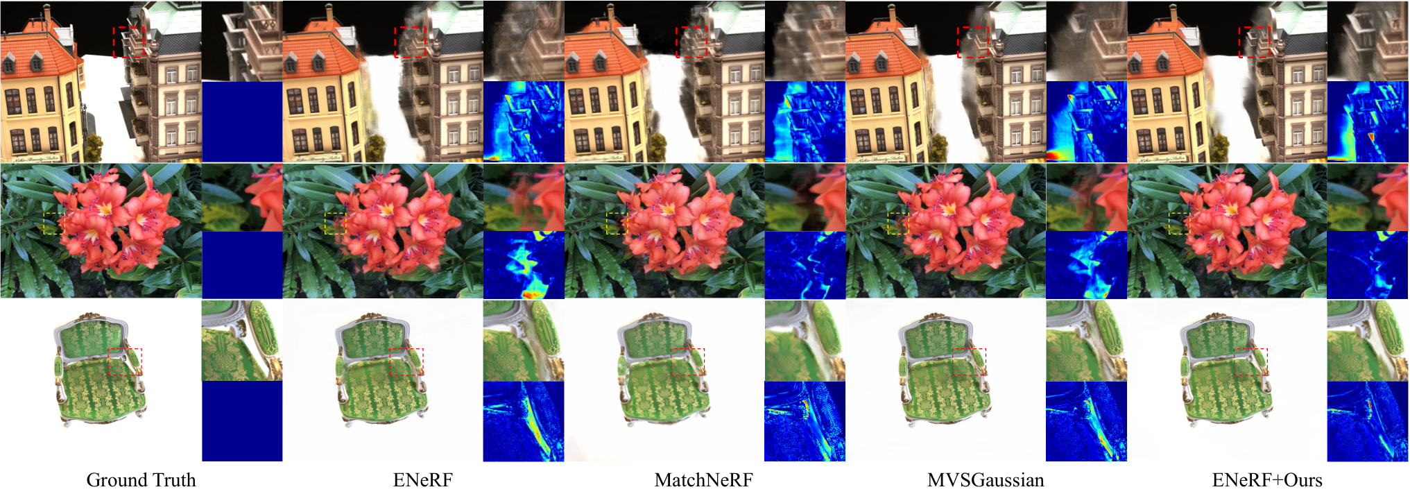
We report quantitative results on the DTU test set in Tab. 1. Additional results on two other datasets are provided in Tab. 2. Notably, ENeRF [22] and MVSGaussian [24] achieve promising speeds by sampling only 1-2 points per ray, while other methods experience slower inference times due to the large number of samples required for accurate reconstruction. We can see that ENeRF+Ours ( $2\times 2$ ) improves PSNR by 1.27 dB and increases FPS by 47% compared to original ENeRF on DTU. Additionally, ENeRF+Ours ( $4\times 4$ ) demonstrates better performance with over twice the speed of the original ENeRF. Performance is not significantly impacted by bundle size. For MVSGaussian+Ours, improvements are limited due to fewer sampling points and dependency on additional post-processing network layers; further performance gains may require a more integrated approach. Thanks to our efficient depth-guided bundle sampling strategy, ENeRF+Ours achieves competitive performance compared to state-of-the-art approaches, while also maintaining high inference speeds. The ability to adjust bundle size provides flexibility, allowing our method to balance speed and quality across different practical applications. Qualitative results in Fig. 4 show that ENeRF+Ours ( $2\times 2$ ) generates high-quality views with enhanced scene detail and fewer artifacts.

5.3 Ablations and Analysis

We conduct a series of ablation studies to evaluate the effectiveness of our design. For efficiency, we limited our experiments to a 3-view configuration on the DTU dataset, employing bundle sizes of $2\times 2$ and $4\times 4$ on ENeRF [22].

Sphere		✗	✓	✓	✓	✓
Sampling
Adaptive		✓	✗	✓	✓	✓
Sampling
Joint Bundle		✓	✓	✓	✗	✓
Representation
Ray-Specific		✓	✓	✗	✓	✓
Representation
$2\times 2$	PSNR $\uparrow$	27.66	28.85	28.47	27.83	28.86
	SSIM $\uparrow$	0.949	0.964	0.958	0.959	0.964
	LPIPS $\downarrow$	0.090	0.076	0.078	0.933	0.073
	FPS $\uparrow$	29.2	17.0	29.4	33.74	28.6
$4\times 4$	PSNR $\uparrow$	25.93	28.06	26.74	27.42	28.21
	SSIM $\uparrow$	0.940	0.954	0.928	0.955	0.957
	LPIPS $\downarrow$	0.105	0.095	0.112	0.099	0.088
	FPS $\uparrow$	44.2	29.1	45.3	49.6	43.6

Table 3: Ablations. The best result is highlighted in bold.

Sampling Strategy.

A unique aspect of our approach is the sphere-based bundle sampling (see Fig. 3), where we sample features from the mipmap of source view feature maps according to the area occupied by each sampled sphere. As shown in Tab. 3, substituting our sphere-based sampling with a pixel-aligned feature extraction at sphere centers results in a PSNR decrease of 1.2 dB.

Depth-Guided Strategy.

The proposed depth-guided adaptive sampling strategy enhances efficiency by not only skipping empty regions but also dynamically adjusting the number of samples according to depth confidence. As illustrated in Fig. 5, this approach allocates more samples at object boundaries and areas with depth discontinuities, where detail is essential. As presented in Tab. 3, this method achieves a 50% increase in FPS while maintaining comparable image quality.

Encoding Strategy.

The joint bundle representation, containing pre-filtered features for the sampled spheres, is inherently smooth and lacks high-frequency details. To enhance detail preservation, we integrate a ray-specific representation that provides pixel-aligned colors for individual ray samples within each sphere. As illustrated in Tab. 3, adding this ray-specific representation boosts PSNR by 0.39 dB for a $2\times 2$ bundle configuration and 1.47 dB for a $4\times 4$ bundle configuration, with slight impact on FPS.

6 Conclusion

We proposed a novel bundle sampling strategy for generalizable novel view synthesis, inspired by plenoptic sampling theory to exploit the piece-wise smoothness of natural scenes. By grouping adjacent rays into bundles and sampling collectively, our approach reduces sampling redundancy while preserving rendering quality. Additionally, our depth-guided adaptive sampling method further optimizes efficiency by dynamically adjusting the number of samples based on depth confidence, concentrating samples at complex regions such as object boundaries and depth discontinuities. Applied to existing methods, our method achieved significant improvements in speed and fidelity. Experimental results on multiple datasets show that our method provides competitive quality with a substantial speed advantage over existing generalizable radiance field models. The flexibility to adjust bundle size also enables trade-offs between speed and quality, broadening its practical applicability to high-resolution, real-time applications.

References

[1] H. Aanæs, R. R. Jensen, G. Vogiatzis, E. Tola, and A. B. Dahl (2016) Large-scale data for multiple-view stereopsis. International Journal of Computer Vision 120, pp. 153–168. Cited by: Figure 1, Figure 1, §5.1, Table 1.
[2] J. T. Barron, B. Mildenhall, M. Tancik, P. Hedman, R. Martin-Brualla, and P. P. Srinivasan (2021) Mip-nerf: a multiscale representation for anti-aliasing neural radiance fields. In Proceedings of the IEEE/CVF international conference on computer vision, pp. 5855–5864. Cited by: §4.1.2.
[3] J. T. Barron, B. Mildenhall, D. Verbin, P. P. Srinivasan, and P. Hedman (2022) Mip-nerf 360: unbounded anti-aliased neural radiance fields. In Proceedings of the IEEE/CVF conference on computer vision and pattern recognition, pp. 5470–5479. Cited by: §4.1.2.
[4] J. Cao, H. Wang, P. Chemerys, V. Shakhrai, J. Hu, Y. Fu, D. Makoviichuk, S. Tulyakov, and J. Ren (2023) Real-time neural light field on mobile devices. In Proceedings of the IEEE/CVF Conference on Computer Vision and Pattern Recognition, pp. 8328–8337. Cited by: §2.
[5] J. Chai, X. Tong, S. Chan, and H. Shum (2000) Plenoptic sampling. In Proceedings of the 27th annual conference on Computer graphics and interactive techniques, pp. 307–318. Cited by: §1, §1, §3.
[6] E. R. Chan, C. Z. Lin, M. A. Chan, K. Nagano, B. Pan, S. De Mello, O. Gallo, L. J. Guibas, J. Tremblay, S. Khamis, et al. (2022) Efficient geometry-aware 3d generative adversarial networks. In Proceedings of the IEEE/CVF conference on computer vision and pattern recognition, pp. 16123–16133. Cited by: §3.
[7] D. Charatan, S. L. Li, A. Tagliasacchi, and V. Sitzmann (2024) Pixelsplat: 3d gaussian splats from image pairs for scalable generalizable 3d reconstruction. In Proceedings of the IEEE/CVF Conference on Computer Vision and Pattern Recognition, pp. 19457–19467. Cited by: §2.
[8] A. Chen, Z. Xu, A. Geiger, J. Yu, and H. Su (2022) Tensorf: tensorial radiance fields. In European conference on computer vision, pp. 333–350. Cited by: §2.
[9] A. Chen, Z. Xu, F. Zhao, X. Zhang, F. Xiang, J. Yu, and H. Su (2021) Mvsnerf: fast generalizable radiance field reconstruction from multi-view stereo. In Proceedings of the IEEE/CVF international conference on computer vision, pp. 14124–14133. Cited by: Figure 1, Figure 1, §1, §2, §5.1, §5.1, Table 1, Table 2, Table 2.
[10] Y. Chen, H. Xu, Q. Wu, C. Zheng, T. Cham, and J. Cai (2023) Explicit correspondence matching for generalizable neural radiance fields. arXiv preprint arXiv:2304.12294. Cited by: Figure 1, Figure 1, §2, Figure 4, Figure 4, §5.1, Table 1, Table 2, Table 2.
[11] Z. Chen, T. Funkhouser, P. Hedman, and A. Tagliasacchi (2023) Mobilenerf: exploiting the polygon rasterization pipeline for efficient neural field rendering on mobile architectures. In Proceedings of the IEEE/CVF Conference on Computer Vision and Pattern Recognition, pp. 16569–16578. Cited by: §1.
[12] J. Chibane, A. Bansal, V. Lazova, and G. Pons-Moll (2021) Stereo radiance fields (srf): learning view synthesis for sparse views of novel scenes. In Proceedings of the IEEE/CVF Conference on Computer Vision and Pattern Recognition, pp. 7911–7920. Cited by: §1, §2.
[13] S. Fridovich-Keil, A. Yu, M. Tancik, Q. Chen, B. Recht, and A. Kanazawa (2022) Plenoxels: radiance fields without neural networks. In Proceedings of the IEEE/CVF conference on computer vision and pattern recognition, pp. 5501–5510. Cited by: §1, §2.
[14] T. Hu, S. Liu, Y. Chen, T. Shen, and J. Jia (2022) Efficientnerf efficient neural radiance fields. In Proceedings of the IEEE/CVF Conference on Computer Vision and Pattern Recognition, pp. 12902–12911. Cited by: §1, §2.
[15] W. Hu, Y. Wang, L. Ma, B. Yang, L. Gao, X. Liu, and Y. Ma (2023) Tri-miprf: tri-mip representation for efficient anti-aliasing neural radiance fields. In Proceedings of the IEEE/CVF International Conference on Computer Vision, pp. 19774–19783. Cited by: §4.1.2, §4.1.
[16] M. M. Johari, Y. Lepoittevin, and F. Fleuret (2022) Geonerf: generalizing nerf with geometry priors. In Proceedings of the IEEE/CVF Conference on Computer Vision and Pattern Recognition, pp. 18365–18375. Cited by: §1, §2.
[17] A. Karnewar, T. Ritschel, O. Wang, and N. Mitra (2022) Relu fields: the little non-linearity that could. In ACM SIGGRAPH 2022 conference proceedings, pp. 1–9. Cited by: §2.
[18] B. Kerbl, G. Kopanas, T. Leimkühler, and G. Drettakis (2023) 3D gaussian splatting for real-time radiance field rendering.. ACM Trans. Graph. 42 (4), pp. 139–1. Cited by: §2.
[19] D. P. Kingma (2014) Adam: a method for stochastic optimization. arXiv preprint arXiv:1412.6980. Cited by: §5.1.
[20] A. Kurz, T. Neff, Z. Lv, M. Zollhöfer, and M. Steinberger (2022) Adanerf: adaptive sampling for real-time rendering of neural radiance fields. In European Conference on Computer Vision, pp. 254–270. Cited by: §2.
[21] J. Li, Z. Feng, Q. She, H. Ding, C. Wang, and G. H. Lee (2021) Mine: towards continuous depth mpi with nerf for novel view synthesis. In Proceedings of the IEEE/CVF International Conference on Computer Vision, pp. 12578–12588. Cited by: §1, §2.
[22] H. Lin, S. Peng, Z. Xu, Y. Yan, Q. Shuai, H. Bao, and X. Zhou (2022) Efficient neural radiance fields for interactive free-viewpoint video. In SIGGRAPH Asia 2022 Conference Papers, pp. 1–9. Cited by: Figure 1, Figure 1, §1, §1, §2, §2, §3, Figure 2, Figure 2, §4.2, §4.3, §4, Figure 4, Figure 4, §5.1, §5.1, §5.1, §5.2, §5.3, Table 1, Table 2, Table 2.
[23] L. Liu, J. Gu, K. Zaw Lin, T. Chua, and C. Theobalt (2020) Neural sparse voxel fields. Advances in Neural Information Processing Systems 33, pp. 15651–15663. Cited by: §2.
[24] T. Liu, G. Wang, S. Hu, L. Shen, X. Ye, Y. Zang, Z. Cao, W. Li, and Z. Liu (2024) MVSGaussian: fast generalizable gaussian splatting reconstruction from multi-view stereo. In European Conference on Computer Vision, pp. 37–53. Cited by: Figure 1, Figure 1, §1, §2, §3, §4.2, §4.3, §4, Figure 4, Figure 4, §5.1, §5.1, §5.1, §5.2, Table 1, Table 2, Table 2.
[25] T. Liu, X. Ye, M. Shi, Z. Huang, Z. Pan, Z. Peng, and Z. Cao (2024) Geometry-aware reconstruction and fusion-refined rendering for generalizable neural radiance fields. In Proceedings of the IEEE/CVF Conference on Computer Vision and Pattern Recognition, pp. 7654–7663. Cited by: §1, §2, §3, §4.2.
[26] Y. Liu, S. Peng, L. Liu, Q. Wang, P. Wang, C. Theobalt, X. Zhou, and W. Wang (2022) Neural rays for occlusion-aware image-based rendering. In Proceedings of the IEEE/CVF Conference on Computer Vision and Pattern Recognition, pp. 7824–7833. Cited by: §1, §2.
[27] B. Mildenhall, P. P. Srinivasan, R. Ortiz-Cayon, N. K. Kalantari, R. Ramamoorthi, R. Ng, and A. Kar (2019) Local light field fusion: practical view synthesis with prescriptive sampling guidelines. ACM Transactions on Graphics (ToG) 38 (4), pp. 1–14. Cited by: §5.1, Table 2.
[28] B. Mildenhall, P. P. Srinivasan, M. Tancik, J. T. Barron, R. Ramamoorthi, and R. Ng (2020) NeRF: representing scenes as neural radiance fields for view synthesis. In ECCV, Cited by: §1, §5.1, Table 2.
[29] T. Müller, A. Evans, C. Schied, and A. Keller (2022) Instant neural graphics primitives with a multiresolution hash encoding. ACM transactions on graphics (TOG) 41 (4), pp. 1–15. Cited by: §1, §2.
[30] T. Neff, P. Stadlbauer, M. Parger, A. Kurz, J. H. Mueller, C. R. A. Chaitanya, A. Kaplanyan, and M. Steinberger (2021) DONeRF: towards real-time rendering of compact neural radiance fields using depth oracle networks. In Computer Graphics Forum, Vol. 40, pp. 45–59. Cited by: §1, §2.
[31] P. Nguyen-Ha, L. Huynh, E. Rahtu, J. Matas, J. Heikkil, et al. (2023) Cascaded and generalizable neural radiance fields for fast view synthesis. IEEE Transactions on Pattern Analysis and Machine Intelligence. Cited by: §1, §2, §5.1, Table 1, Table 2.
[32] R. Ramamoorthi (2024) Sampling for view synthesis: from local light field fusion to neural radiance fields and beyond. arXiv preprint arXiv:2408.04586. Cited by: §3.
[33] C. Sun, M. Sun, and H. Chen (2022) Direct voxel grid optimization: super-fast convergence for radiance fields reconstruction. In Proceedings of the IEEE/CVF conference on computer vision and pattern recognition, pp. 5459–5469. Cited by: §2.
[34] J. Sun, T. Wu, and L. Gao (2024) Recent advances in implicit representation-based 3d shape generation. Visual Intelligence 2 (1), pp. 9. Cited by: §1.
[35] S. Szymanowicz, C. Rupprecht, and A. Vedaldi (2024) Splatter image: ultra-fast single-view 3d reconstruction. In Proceedings of the IEEE/CVF Conference on Computer Vision and Pattern Recognition, pp. 10208–10217. Cited by: §2.
[36] T. Tanay and M. Maggioni (2024) Global latent neural rendering. In Proceedings of the IEEE/CVF Conference on Computer Vision and Pattern Recognition, pp. 19723–19733. Cited by: §1, §2, §5.1, Table 1.
[37] A. Trevithick and B. Yang (2021) Grf: learning a general radiance field for 3d representation and rendering. In Proceedings of the IEEE/CVF International Conference on Computer Vision, pp. 15182–15192. Cited by: §1, §2.
[38] Z. Wan, C. Richardt, A. Božič, C. Li, V. Rengarajan, S. Nam, X. Xiang, T. Li, B. Zhu, R. Ranjan, et al. (2023) Learning neural duplex radiance fields for real-time view synthesis. In Proceedings of the IEEE/CVF Conference on Computer Vision and Pattern Recognition, pp. 8307–8316. Cited by: §2.
[39] P. Wang, X. Chen, T. Chen, S. Venugopalan, Z. Wang, et al. (2023) Is attention all that nerf needs?. Proceedings of the International Conference on Learning Representations (ICLR). Cited by: §1, §2, §5.1, Table 1, Table 2, Table 2.
[40] Q. Wang, Z. Wang, K. Genova, P. P. Srinivasan, H. Zhou, J. T. Barron, R. Martin-Brualla, N. Snavely, and T. Funkhouser (2021) Ibrnet: learning multi-view image-based rendering. In Proceedings of the IEEE/CVF conference on computer vision and pattern recognition, pp. 4690–4699. Cited by: Figure 1, Figure 1, §1, §2, §5.1, Table 1, Table 2.
[41] Z. Wang, A. C. Bovik, H. R. Sheikh, and E. P. Simoncelli (2004) Image quality assessment: from error visibility to structural similarity. IEEE transactions on image processing 13 (4), pp. 600–612. Cited by: §5.1.
[42] Z. Wang, T. Shen, M. Nimier-David, N. Sharp, J. Gao, A. Keller, S. Fidler, T. Müller, and Z. Gojcic (2023) Adaptive shells for efficient neural radiance field rendering. ACM Transactions on Graphics (TOG) 42 (6), pp. 1–15. Cited by: §1.
[43] H. Xu, A. Chen, Y. Chen, C. Sakaridis, Y. Zhang, M. Pollefeys, A. Geiger, and F. Yu (2024) Murf: multi-baseline radiance fields. In Proceedings of the IEEE/CVF Conference on Computer Vision and Pattern Recognition, pp. 20041–20050. Cited by: Figure 1, Figure 1, §1, §5.1, Table 1, Table 2, Table 2.
[44] A. Yu, R. Li, M. Tancik, H. Li, R. Ng, and A. Kanazawa (2021) Plenoctrees for real-time rendering of neural radiance fields. In Proceedings of the IEEE/CVF International Conference on Computer Vision, pp. 5752–5761. Cited by: §2.
[45] A. Yu, V. Ye, M. Tancik, and A. Kanazawa (2021) Pixelnerf: neural radiance fields from one or few images. In Proceedings of the IEEE/CVF conference on computer vision and pattern recognition, pp. 4578–4587. Cited by: §1, §2, §5.1, Table 1, Table 2.
[46] R. Zhang, P. Isola, A. A. Efros, E. Shechtman, and O. Wang (2018) The unreasonable effectiveness of deep features as a perceptual metric. In Proceedings of the IEEE conference on computer vision and pattern recognition, pp. 586–595. Cited by: §5.1.
[47] S. Zheng, B. Zhou, R. Shao, B. Liu, S. Zhang, L. Nie, and Y. Liu (2024) Gps-gaussian: generalizable pixel-wise 3d gaussian splatting for real-time human novel view synthesis. In Proceedings of the IEEE/CVF Conference on Computer Vision and Pattern Recognition, pp. 19680–19690. Cited by: §2.