Beyond separability: convergence rate of vanishing viscosity approximations to mean field games via FBSDE stability
Abstract.
We study the vanishing viscosity approximation to mean field games (MFGs) in with a nonlocal and possibly non-separable Hamiltonian. We prove that the value function converges at a rate of , where is the diffusivity constant, which matches the classical convergence rate of vanishing viscosity for Hamilton-Jacobi (HJ) equations. The same rate is also obtained for the approximation of the distribution of players as well as for the gradient of the value function. The proof is a combination of probabilistic and analytical arguments by first analyzing the forward-backward stochastic differential equation associated with the MFG, and then applying a general stability result for HJB equations. Applications of our result to -player games, mean field control, and policy iteration for solving MFGs are also presented.
Key words: convergence rate, Fokker-Planck equation, forward-backward stochastic differential equation, mean field control, mean field games, non-separable Hamiltonian, nonlocal coupling, policy iteration, vanishing viscosity approximation.
1. Introduction
Mean field games (MFGs) were simultaneously proposed by Lasry and Lions in [45, 46, 47], and by Huang, Malhame, and Caines in [41], for the purpose of modeling a game with a large number of players whose decisions are influenced by the distribution of the other players. Due to the large number of players, each player is assumed to have an infinitesimally small influence on all of the other players. Moreover, if we assume that all players act rationally (meaning that they each solve an optimization problem of some cost functional and act as though all other players are also playing rationally), then the system is said to be in a Nash equilibrium. Now suppose that the agents are playing on the state space . Then, one of the most common formulations of MFGs is as a system of coupled partial differential equations (PDEs), of which the first is a Hamilton-Jacobi-Bellman (HJB) equation solved by , and the second is a Fokker-Planck equation solved by a flow of probability measures on :
| (1.1) |
where is the idiosyncratic noise intensity 11 1 The coefficient is also called the diffusivity constant., is a possibly non-separable Hamiltonian, is the terminal cost, and is the initial distribution. When , the system is of second order. The system obtained by sending is called the vanishing viscosity limit, which is of first order. Refer to Section 1.1 for a literature review on the well-posedness of MFGs (1.1).
Second-order MFGs are widely used to model complex systems in economics [1, 18, 53] and engineering [28, 40]. Recently, there has been a surge of interest in first-order MFG models, where the state evolves according to deterministic dynamics. Examples include the traffic flow of pedestrian crowds and autonomous vehicles [35, 39], and Proof-of-Stake cryptocurrency mining [64, Section 5]. As prior works have noted, such as in [39], traditional methods (e.g., Newton’s method) for solving first-order MFGs tend to be numerically unstable. Various approaches [14, 15, 50] have recently been proposed to address such problems in solving first-order MFGs with a separable Hamiltonian (see (1.2) below), but with no quantitative guarantees. An obvious approach, as already suggested in [2], is to add a small second-order perturbation that corresponds to the addition of a small idiosyncratic noise, and then to solve the resulting second-order MFG 22 2 This approach is also reminiscent of the Lax-Friedrichs approximation scheme to first-order equations, where numerical viscosity is with as the space-time discretization (see e.g., [22, 23, 58]).. However, the price of gaining numerical stability from the perturbation is to introduce a source of error depending on the noise intensity . Denoting for the value function of the first-order MFG, one would expect from the classical theory of Hamilton-Jacobi equations (see e.g., [24, Section IV]) that as , in some topology. But the classical theory of viscosity solutions cannot immediately provide a convergence rate with respect to for MFGs on account of the coupling with the Fokker-Planck equation.
The purpose of this paper is to provide a quantitative convergence rate to vanishing viscosity limit of the MFG (1.1) with a general, possibly non-separable Hamiltonian. Previous work [62] has studied the convergence rate of vanishing viscosity limits of MFGs with a separable Hamiltonian on the torus ; see the end of Sections 1.1 and Remark 2.8 for discussions. Now let us briefly describe our results: we prove that under suitable conditions on the model parameters, for any compact set ,
for some constant . Under certain regularity conditions, we can show that grows at most quadratically in the diameter of . In other words, at a rate of in the topology of uniform convergence on compact sets (Theorem 4.4), which matches the convergence rate from the classical viscosity theory of Hamilton-Jacobi equations. As intermediary steps, we prove: (1) when the initial condition is bounded, converges to at a rate of in the metric, for any large enough bounded set (Theorem 3.3), as well as in the metric, uniformly in (Corollary 3.5), and (2) converges to in the -Wasserstein distance (Corollary 3.4). Our analysis specifically requires neither the Lasry-Lions nor the displacement monotonicity condition; see Remark 2.8 for a discussion. In Section 5, we also show how to apply our result to various problems, such as particle system approximations and policy iteration for solving MFGs.
Here we give a quick outline of the proof, which is a combination of probabilistic and analytical arguments. From the classical stability theory of PDEs, one might suspect that the difference between and is controlled by the difference in the coefficients, i.e., , , and . However, the dependence on the measure in the first four terms complicates the analysis, because and satisfy their own PDEs that depend on and , respectively. We avoid this issue by instead analyzing the forward-backward stochastic differential equation (FBSDE) system (defined in (2.3)) associated with the MFG system (1.1). Our analysis consists of three steps:
- (1)
Using the FBSDE representation of the MFG, and temporarily assuming that the initial condition is bounded, we control the difference between and in terms of and (Lemma 3.2) for some large enough set .
- (2)
- (3)
Finally, we comment that while we mostly use the and distances in the statements of our results, we expect that our results should easily extend to and distances when the initial distribution is only -integrable, for .
Organization of the paper: The remainder of this paper is organized as follows. Section 1.1 provides a literature review on MFGs, and compares the result in this paper with prior work. In Section 2, we formally define the problem and collect some assumptions for our result. Section 3 proves the convergence rate of and , and Section 4 proves the convergence rate of . In Section 5, we give several applications of our result. Examples and numerical experiments are presented in Section 6. We make some concluding remarks in Section 7.
1.1. Literature review
The well-posedness of MFGs has been studied extensively, particularly for the case of a separable Hamiltonian, in which the momentum and the measure arguments are additively separated:
| (1.2) |
Here can either be a local or nonlocal function of the measure argument. In the separable, local case and when , [13, 11, 31] are some of the major works proving the well-posedness. In the separable, nonlocal case and when , [12] proved well-posedness of the MFG system, provided that the Lasry-Lions monotonicity condition holds.
The separable case is a strong structural assumption, upon which much of the previous literature relied. However, many applications may go beyond this assumption. In the economic model proposed by [1, 53], despite the model of the agent being relatively simple to formulate, such an agent corresponds to a MFG whose Hamiltonian is not separable. Another example is provided by [64], where the Hamiltonian has a term containing the product of the price process (which is a function of the player distribution) and the action of the player. Finally, [3] is one of the works that models mean field games with congestion, where players are penalized based on the density of other players at the current position; as a result of congestion penalizing movement, the Hamiltonian some function of the momentum divided by another function of the density. In order to make sense of the MFGs arising in these applications, the well-posedness of MFGs with a non-separable Hamiltonian must first be established. A breakthrough was made by [34], and later [52], for their proposal of a new condition, called displacement monotonicity, under which well-posedness of the MFG system (1.1) can be proved for all . To the best of our knowledge, the work that proves well-posedness under the least restrictive regularity assumptions on and is [5], whose main assumption, other than displacement monotonicity, is the uniform boundedness of the second derivatives of and .
Some earlier works take a probabilistic approach to MFGs as well. [17] considers a probabilistic formulation of the MFG, where the volatility is uncontrolled. Their Remark is similar to our FBSDE system (2.3), though our equation of the adjoint process is for the gradient of the value function, not for the value function itself. The later work of [43] also studies MFGs from a probabilistic perspective, and they prove the existence, though not its uniqueness, of a MFG solution where the volatility is controlled. See [16] for further developments in this direction.
While the classical setting of the convergence rate of vanishing viscosity approximations to pure Hamilton-Jacobi equations has been studied extensively, two recent papers [20, 19] were motivated by applications to mean-field control to provide an even sharper convergence rate of . Central to both papers is an estimate of the integral of the Laplacian of the value function, with respect to the solution of an adjoint equation [49], over in [20] and in [19]. Although they do not apply their results to mean field games, especially ones with a more general, non-separable Hamiltonian (however, in their setting, ”non-separability” would mean that the Hamiltonian’s momentum and time arguments cannot be separated like Equation (1.2)), it would be interesting to apply their technique to our setting as well.
Comparison to previous work: The only previous work addressing the convergence rate of vanishing viscosity approximations to MFGs is [62]. Its main assumption is that of a separable Hamiltonian, which (along with the terminal cost function) satisfies the Lasry-Lions monotonicity condition. In contrast, we do not assume any monotonicity condition until one is needed for the well-posedness of the MFG system (1.1). Moreover, our result addresses the case of a non-separable Hamiltonian which is nonlocal in the measure argument. We prove that the convergence rate for is in for any compact set , which improves upon their rate in . This (partially) solves Problem 4(a) in [62] for MFGs with nonlocal and possibly non-separable Hamiltonians.
2. Notations, Assumptions and Problem Formulation
2.1. Notations
For a metric space , let be the space of functions mapping to , which are -times differentiable and whose -th order derivatives are continuous. is the subset of whose functions are compactly supported. If , then for , refers to , and refers to . In particular, and do not include the partial derivatives with respect to .
For , a generic measure space , and a metric space (which will almost always be Euclidean space in this paper), is the space of -valued functions whose -th power is integrable with respect to , i.e., all such that . If , then is the space of functions such that there exists a constant satisfying ; the infimum of all such constants is denoted by . If we omit a -field , then it should be clear from context whether it is the Borel -field or an element of some filtration generated by a stochastic process, for instance. We might also omit specifying the measure when it is clear whether it is, for example, Lebesgue measure on or a probability measure on some sample space . If we do not specify a metric space , then it should be taken . We will also make use of spaces of functions mapping to , denoted by consisting of functions such that there exists a with almost everywhere with respect to the Lebesgue measure on ( is the Euclidean norm on ). If is replaced by , the space of by matrices, then is replaced by the operator norm on matrices.
Now let be a probability space. For a random variable , is the law of with respect to . For , we write for the space of probability measures with finite -th moment, i.e., . On , we define the -Wasserstein distance :
We also introduce the concept of the Wasserstein gradient of a function . For a more extensive introduction, please refer to [16, Chapter 5], [12, Section 1.4], or [10, Section 6]. For , the Wasserstein gradient of at is denoted by , and it is an element of the closure of gradients of functions, with respect to the metric. Moreover, it follows from [12, Definition 1.11] 33 3 The Wasserstein gradient is defined slightly differently in [12, Definition 1.11], but Equation 2.1 can be recovered by taking the transport plan to be in their notation. that satisfies: for all -valued random variables and ,
| (2.1) |
Finally, for , the symbol , or means that is bounded from above, as some problem parameter tends to or . Similarly, means that is bounded from below and from above, as some problem parameter tends to or .
2.2. Assumptions
Unless otherwise said, we work on a filtered probability space , , generated by a standard -dimensional Brownian motion . Let be the Hamiltonian, and be the terminal cost function. We need the following Lipschitz and regularity conditions on and , as well as a convexity assumption on for the FBSDE representation (2.3) and a well-posedness assumption.
Assumption 2.1 (Regularity of ).
The derivatives , , , , , and exist. Moreover, despite not specifying a measure on , we say that , , and have finite norms on their respective domains in the sense that:
and are Lipschitz in the measure argument with Lipschitz constants and : for all and ,
Finally, we borrow these assumptions from [52, (2.5), (2.6)]: , uniformly in , and is continuous in with respect to , locally uniformly on .
Assumption 2.2 (Convexity of ).
[52, (2.7)] is uniformly convex in : there exists some such that . Also, for each , there exists a constant such that for all , .
Assumption 2.3 (Regularity of ).
The derivatives , , and exist. Moreover, despite not specifying a measure on , we say that has finite norm in the sense that:
Again, we borrow these assumptions from [52]: is Lipschitz in the measure argument with respect to , and we denote its Lipschitz constant by : for all and ,
Finally, uniformly in , and is continuous with respect to , locally uniformly in .
Assumption 2.4.
The initial condition is an element of .
Assumption 2.5.
The McKean-Vlasov FBSDE (2.3) is stable with respect to the initial condition. To be precise, let have laws satisfying Assumption 2.4. Let the solution to Equation (2.3) with initial condition be denoted as ; similarly, let denote the solution to Equation (2.3) but with initial condition . We assume that for some constant depending only on and the Lipschitz constants of and ,
| (2.2) |
This assumption is satisfied by FBSDEs covered by certain conditions sufficient for the well-posedness of the FBSDE associated with the MFG, such as displacement monotonicity [52, Theorem 4.5]. We would like to mention that the specific structure that displacement monotonicity is not the key to our results, as any other condition that implies the property of stability with respect to the initial condition could replace displacement monotonicity without changing our results.
Assumption 2.6.
Remark 2.7.
We present two classes of Hamiltonians that satisfy Assumptions 2.1 and 2.2.
- (1)
- (2)
- (3)
Consider the one-dimensional example
for , . If are bounded, then satisfies Assumptions 2.1 and 2.2, and if there is some such that for each . This example is inspired by [64], despite its Hamiltonian being time-dependent. While our assumptions do not allow for time-varying Hamiltonians, we expect our results to extend to them under suitable regularity conditions.
- (4)
For a function and a mollifier (i.e., its derivatives up to the second order are bounded and compactly supported), , and , define
If are bounded, and if is large enough, then Assumptions 2.1 and 2.2 are satisfied. This example is motivated by non-separable Hamiltonians from MFGs modeling congestion [3]. The idea behind the convolution of with is to transform the Hamiltonian that is usually encountered in MFGs with congestion from a local one into a nonlocal one. From a modeling perspective, it should be interpreted as agents not only taking into account the density of agents at their current position, but also the density of agents in some compact set around the agent’s position. Ideally we would allow to be unbounded, such as setting as in [3], but this would violate the assumption that as well as the assumption of uniform convexity if .
Our assumptions largely agree with those in [5] (namely, Assumptions 2.6(1) and 2.7(1) therein). To reiterate, [5] is, to the best of our knowledge, the work with the least restrictive regularity assumptions that guarantee well-posedness of the master equation.
As discussed in [52, Section 3], Assumption 2.6 can be satisfied by MFGs that do not necessarily possess displacement monotone or . Indeed, we allow any and that satisfy any conditions that are sufficient to guarantee well-posedness (and do not contradict Assumptions 2.1–2.4). See, for example, [37, 54] for additional conditions sufficient for well-posedness that are beyond the Lasry-Lions and displacement monotonicity conditions.
Remark 2.8 (Comparison with [62]).
We compare our assumptions to those of [62] in greater detail. In terms of regularity, their condition (H1’) on the norm of the coupling says that the coupling must have bounded first and second derivatives, which is slightly stronger than ours (we allow for to be unbounded). Their condition (H2’), that the second-order derivatives of are locally bounded, is of course not as strong as uniform boundedness. Their condition (H3’) is stronger than ours, which requires that the norm of the terminal cost is bounded, while we only require that be Lipschitz in the measure argument with respect to . Finally, (H4’) and (H4”) do not seem to be directly comparable to the regularity of L-derivatives. However, observe that if the condition (in H4’ and H4”):
were replaced with
then they would have achieved the same convergence rate as we did.
Moreover, we did not find necessary to assume the monotonicity conditions that [62] imposed on their Hamiltonian and coupling. For instance, we could impose any of the four conditions in [37] that guarantee well-posedness of the MFG system, while [62] did require the Lasry-Lions monotonicity condition for their proof 44 4 The Lasry-Lions monotonicity condition is needed in their equations (6.10) and (6.11).. Most importantly, [62] relied on the separable Hamiltonian structure, and their proof technique seems difficult to adapt to the non-separable case on account of the dual equation technique [49].
2.3. Problem Formulation
Let be a filtered probability space for some time horizon , where the filtration is generated by a standard -dimensional Brownian motion . For a sequence of measures , a representative agent takes a path through , which satisfies the SDE:
for some initial position , initial time , and adapted stochastic process (referred to as the control). Its goal is to minimize the following cost functional :
over all controls . Here, the Lagrangian is a running cost function that is the Legendre transform of in the second variable, is a terminal cost function, and is the idiosyncratic noise intensity faced by each player. Let . From classical optimal control, if all players play optimally in the sense of a Nash equilibrium, then at time and position , each player chooses the action , defined by
and we can set the sequence of measures to be , the solution to the Fokker-Planck equation in Equation (1.1). As both and are fixed, and since our focus is on the dependence of on , we replace and in by the noise intensity . We use to refer to the stochastic process representing the path of the agent, and we use to refer to the law of . Moreover, the pair solves the coupled PDEs (1.1) in the following sense:
Definition 2.9.
[52, Definition 3.2] We say that is a solution to the MFG system 1.1 if
- (1)
for all , the Lipschitz constant of restricted to any compact set is finite, is a viscosity solution to the HJB equation, and .
- (2)
is continuous, and solves the Fokker-Planck equation in the distributional sense: for all test functions , the following equation holds:
Moreover, satisfies the initial condition:
It is worth noting that from [52, Lemma 3.4], there is an estimate for which is uniform in : . Moreover, according to [52, Theorem 4.1], under Assumption 2.2, the MFG (1.1) has an FBSDE representation:
| (2.3) |
and it has a strong solution. The first SDE describes the state dynamics of an agent playing in a Nash equilibrium. The key to our analysis is the fact that is a decoupling field for the FBSDE (2.3) in the sense that:
The meaning of to the FBSDE is that the SDE for is solved by the gradient of the value function evaluated along the trajectory of a typical agent playing in a Nash equilibrium. Instead of relying on PDE methods such as the dual equation as [62] did, we use a probabilistic approach that hinges on stability properties of the FBSDE (2.3) to derive our main result.
3. Convergence of and
The difficulty of analyzing MFGs with a non-separable Hamiltonian is that without the assumption of separability (1.2), we can no longer analyze each equation separately. However, as discussed previously, we can use the convenient property of the FBSDE (2.3) having as a decoupling field in the sense of Equation (2.3). By substituting Equation (2.3) into the SDE for , we can analyze it separately from the SDE for . Furthermore, because for all , we can get a convergence rate for to in , and hence, in .
Before we state the results, we define the following FBSDE system for and :
| (3.1) |
Its only differences compared to (2.3) is that the initial time is not necessarily and that the initial condition does not need to have the law . To lighten notation, when , we denote by to be the solution to the FBSDE (2.3) or (3.1). For a bounded set , we write to be the event that does not exit between , i.e.
Lemma 3.1.
Let and . If is the solution to Equation (3.1) with and initial condition , then there exists a bounded set such that has probability . It is worth mentioning for future reference the obvious corollary that for any set containing , also has probability .
Proof.
By a standard argument using Grönwall’s inequality, , the definition of , and being a decoupling field,
It follows that has a Lipschitz constant uniform in . By classical ODE theory, is an element of for all . Since the law of is compactly supported, there exists some bounded set such that for all , for all . ∎
Lemma 3.2.
Proof.
Firstly, suppose is defined as above the statement of the lemma: as a bounded set such that for all , . For any and ,
because is locally Lipschitz continuous in , on account of . Now, note that the equation (3.2) is the SDE satisfied by a solution to the component of the FBSDE (3.1), the existence of which is guaranteed by [52, Theorem 4.1] and Assumption 2.2. Using Assumptions 2.1 and 2.3, as well as , we have that for all :
| (3.4) | ||||
where the expectations are finite due to the assumption that . As a result, there exists some constant depending only on and the Lipschitz constants of the gradients of and , such that for all :
where we used the fact that has probability in the first line, the definition of and in the second line, and and Equation (3.4) in the third line. By Grönwall’s inequality, there exists another constant such that
Using the fact that the right-hand side is non-decreasing in as well as the uniformity of in yields the conclusion. ∎
The previous result hints that in order to quantify the convergence of to , it suffices to control the convergence of to in . In the following theorem, we obtain a convergence rate of for to by using its role as the decoupling field.
Theorem 3.3.
Let and be solutions to the value function component of the MFG system (1.1) with and , respectively. Suppose that Assumptions 2.1 – 2.3 hold and that . Then there exists a constant , where the dependence on and is only through the bounds on the second-order derivatives of and , and some bounded set that is large enough for to have probability , such that
Proof.
Firstly, due to Lemma 3.1, we know that such a exists and that the range of is contained in . Denote by and the solutions to the FBSDE (3.1) with the initial condition , , and and respectively. We have and for almost every , since we can take conditional expectation of the and components of Equation (3.1), conditioned on the event that , as in [52, (4.13)]. Using the uniform convexity of in from Assumption 2.2, we have that for ,
By the triangle inequality, we get:
| (3.5) |
Using Lemma 3.2 and Assumption 2.3, we can bound the first term in (3.5) by
| (3.6) | ||||
By Assumption 2.1, there is some constant depending on the Lipschitz constants of in , , and , as well as on , such that we can bound the second term in (3.5) as:
| (3.7) | ||||
By applying Lemma 3.2 to , using , and collecting the time integral of into a supremum, we can continue from the last line in Equation (3.7) to get:
| (3.8) | ||||
In the above computations, the value of may change from line to line but only depends on and the Lipschitz constants of the relevant gradients of and . Therefore, after taking the supremum over all and combining (3.6) and (3.8), Equation (3.5) is bounded by
Then we apply Grönwall’s inequality to find that for another constant still only depending on , , and ,
Since does not depend on , we conclude that . ∎
Corollary 3.4.
Proof.
Let and . Since is square-integrable, there exists some random variable whose range is contained in a bounded set such that .
To explain further why such a exists, consider the sequence of functions , which converges pointwise to as . By the dominated convergence theorem, we can find large enough such that for ,
Take large enough that is contained in . Define the random variable to be the product of and the indicator function of , so that
Thus, if we define to be the closure of the union of and , then is the desired random variable. From now on, we can take to be instead. For , denote and to be the solutions to Equation (2.3) with initial conditions and respectively. and are the solutions to Equation (2.3) with initial conditions and , but for . With the above observations and using the abbreviation for , for all :
| (3.10) | ||||
In Equation (3.10), to transition from the first line to the second, we applied Assumption 2.5 to handle the first and third terms, and we applied Lemma 3.2 to handle the second term; the use of Lemma 3.2 was justified because their initial conditions and were assumed to be bounded. The constant in the second line depended on , , and . To handle the term in the square root in the second line, we applied Theorem 3.3. As promised, in the third line, the dependence of on was only through absorbing into the constant of the second line. Since is arbitrary, the result follows. ∎
The convergence result for may be slightly unsatisfying due to the metric in which it was stated. Thus, although we will not use this result for the rest of the paper, we briefly comment that Assumption 2.5 and Corollary 3.4 enable us to derive a rate of convergence of for in the metric.
Corollary 3.5.
Proof.
The families of random variables , indexed by , are uniformly absolutely continuous in the sense that for all , there exists a such that for all with , we have
since for a constant independent of and depending only on and the supremum over of (which is finite by a standard argument for an SDE whose initial condition is and whose coefficients are Lipschitz in space, uniformly in time, and satisfy a linear growth condition),
for small enough. In combination with , this is equivalent to the uniform integrability of by [55, Theorem 6.5.1]. Moreover, due to Arzela-Ascoli, converges to uniformly on compacts, so converges to in probability. By the Vitali convergence theorem (see, for example, [55, Theorem 6.6.1]),
| (3.11) |
For a constant depending on and on the constant from Assumption 2.5, we obtain
| (3.12) |
where the first inequality is just by the triangle inequality, Fubini’s theorem, and Holder’s inequality. (In fact, we could have written instead of and instead of in everything above without any changes to the proof, which is how convergence in the metric can be proven.) Taking the limit as in Equation (3.12) and then using Equation (3.11), we obtain . ∎
4. Convergence of
We first present a general stability result concerning Hamilton-Jacobi equations with respect to the supremum norm on compact sets. Similar results exist in the literature but are not directly applicable in our scenario 55 5 Closely related results are [57, Propositions 1.4 and 2.1]. However, the former proposition assumed that the solution to their HJ equation was bounded and that it lacked a second-order term, and the latter assumed that the Hamiltonian was bounded in space and time. Another potentially applicable result was [62, Lemma 6.3]. But on account of their formulation not allowing for non-separable Hamiltonians, we also cannot directly apply this lemma.. To informally describe the resul: if two HJ PDEs are well-posed with solutions and , Hamiltonians and , terminal cost functions and , and viscosity parameters and , then the maximum difference between and on any compact set in is bounded by the difference in the coefficients , on that compact set, and a term.
Theorem 4.1.
Let . For , let and be continuous. Suppose that is uniformly convex in the second variable , in the sense that there exist constants such that . Assume that is Lipschitz in the first argument , uniformly in the second and third arguments, i.e. is finite, and additionally assume that is bounded. If the equations
| (4.1) |
are well-posed in the classical sense for with solution , then for any compact set with diameter and for any , there exists a constant growing at most linearly in such that
| (4.2) |
where satisfies for all and grows at most linearly in .
Proof.
Define the costate variable for as , where is the solution to the following ODE
| (4.3) |
In other words, is the optimally controlled trajectory achieving (c.f. Equation (3.1) with ). From the assumption of being bounded, Equation (4.3) is well-posed and defined for all . Let . Due to being bounded on , the sublinear growth of , and the uniform convexity of , we can bound the right-hand side of Equation (4.3) as follows:
| (4.4) |
for some depending on , , and . By a standard application of Grönwall’s inequality, for all ,
| (4.5) |
Defining the right hand side as , the costate variable can be controlled as well: for all : . Denote as the Fenchel conjugate of in the -variable. Because is a sub-optimal trajectory for but is optimal for , in conjunction with the Hopf-Lax representation of , we get the inequality
| (4.6) |
We want to control the integrand in Equation 4.6 by something depending on . Because is the Fenchel conjugate of in the -variable, and because the supremum is attained uniquely due to the uniform convexity of by some solving the equation , it follows that for all ,
| (4.7) |
Due to symmetry, the same equation can be proven with the subscripts swapped. Hence, we can bound with and :
| (4.8) |
The second inequality comes from the fact that (see the definition of the optimizer in the Fenchel conjugate and the fact that it is unique, so that ), using Equation (4.3), and then using and .
Now we need to control ; since the only unknown quantity is , which does not coincide with in general, we are done if we can contain in some ball whose radius depends on for all . Using the uniform convexity of , the fact that is the solution to the equation , and Equation (4.3), we obtain:
| (4.9) |
Because , , and is continuous, we see that the last line is bounded by some constant , and so
| (4.10) |
and due to and being bounded, grows at most linearly in . This yields a bound on , because
| (4.11) |
Therefore, substituting Equation (4.11) into Equation (4.8) and then into the Hopf-Lax representation in Equation 4.6, we obtain:
| (4.12) |
The roles of and were symmetrical and can therefore be swapped, which proves the result. ∎
The following result is well-known (see, for instance, e.g. [62, Lemma 7.1]), but we restate it since we want a precise dependence of its constants on the diameter of the set .
Proposition 4.2.
Let and . Suppose and satisfy the same assumptions as and do in Theorem 4.1. If the equations
| (4.13) |
are well-posed for with solution , then for any compact set , there exists a constant and another constant such that
where grows at most quadratically in .
Proof.
By modifying the proof of [62, Lemma 7.1], taking , using the linear-in- growth of and , and the quadratic-in- growth of and , we find that there exists a constant such that for any compact set ,
Technically, we should take the maximum of and its square, but for the sake of simplicity, we opt to omit this. ∎
Corollary 4.3.
Let and satisfy the assumptions in Theorem 4.1, and let and satisfy the assumptions in Theorem 4.2. Suppose satisfies Equation 4.1 with , and suppose satisfies the second PDE in Equation 4.13 with . Then for any compact set with diameter , there exists a constant growing at most quadratically in , such that
where , , and are as in Theorem 4.1.
Proof.
Now we combine the results in Section 3 with Corollary 4.3 and make some modifications to the proof of Theorem 4.1 that are particular to the case of measure-dependent in order to derive the promised rate of convergence.
Theorem 4.4.
For , suppose the MFG system (1.1) satisfies Assumptions 2.1–2.6, whose solutions for the HJB equation are denoted and .
- (1)
converges uniformly to on compacts at a rate of : for any compact set , there exists a constant depending on the data such that
(4.14) when is small enough.
- (2)
If additionally is Lipschitz in the measure argument with respect to , then for some constant depending on the data that grows at most quadratically in , for all ,
Proof.
In Theorem 4.1, let us specialize to the case where and , so that and . Recall that is the solution to the FBSDE in Equation 2.3 with . Note that is jointly continuous on for any , since for any , is bounded on , due to a Taylor expansion around , Assumption 2.1, and being bounded with respect to . For the same reasons, is bounded on . Noting that is continuous in the measure variable with respect to and that the same argument holds when is replaced with closes the argument for joint continuity of on . It follows that the difference of and on is achieved at some , which we will abbreviate as for convenience. Thus, for and ,
| (4.15) |
The second line is via a Taylor expansion of in the measure variable, which occurs only when and are close enough in - see Corollary 3.4. The third line comes from the same corollary, from Cauchy-Schwartz, and from the Taylor expansion of in and . The fourth line collects the relevant constants into .
Now, we bound more precisely. Recall that comes from Equation (4.9); since , we can identify in Theorem 4.1 with solving Equation (3.1) with and . Continuing from Equation (4.9), we are able to bound as follows:
| (4.16) |
Therefore, is of at most linear growth in , and
| (4.17) |
Now we want to bound , which is achieved for some due to the continuity of in . From Corollary 3.4, for small enough,
| (4.18) |
for some depending on and (and so on , , and by extension). Substituting Equation 4.16 into Equation 4.15, and then substituting Equation 4.18 into the bound provided by Corollary 4.3, we obtain:
| (4.19) |
which concludes the proof of (1).
Remark 4.5.
If it is only assumed that and are continuous in , by the stability of viscosity solutions to the HJB equation, we can conclude that uniformly on compacts, albeit without a rate.
5. Applications
This section provides three applications of our result to -player games, mean field control, and policy iteration.
5.1. -player games
MFGs arise as the limit of -player games as the number of players increases to infinity. Although it is known in various circumstances [29, 32, 44] that the limit is the MFG equilibrium, finding the convergence rate is a separate and difficult problem. The twin papers [26, 27] seem to comprise the most recent progress on determining the convergence rate. However, their results cannot be directly applied to the -player convergence rate problem if the agents follow deterministic dynamics, because one of their assumptions, namely A.2 in both papers, is that the volatility coefficient is non-degenerate 66 6 When we say that the volatility is non-degenerate, we mean that its minimum eigenvalue is positive. Moreover, if the minimum eigenvalue of is allowed to vanish, then their upper bounds for the distance between the probability distribution of the finite player system and that of the MFG limit become infinite.. Here we apply Corollary 3.4 to approximate the probability flow of the first-order MFG by the empirical measures of an -player system with non-degenerate volatility.
To simplify our discussion, we only consider the linear drift . So by [27, (2.6)], the value functions of all players, , satisfy the -player system of PDEs whose -th component is:
where is the empirical measure of . Specializing to the case of , the -th player’s dynamics are:
| (5.1) |
where are independent -dimensional Brownian motions and is the (random) empirical measure of the -player system (5.1) at time :
| (5.2) |
Corollary 5.1.
Proof.
As a result of Corollary 5.1, we obtain the population level to approximate the probability flow of the first-order MFG via large player system. Assume that an accuracy of is needed, i.e., . Then we set:
| (5.6) |
Here we assume that are given, so only depends on . A close scrutiny of the proofs (in particular, Equations 4.16 and 4.17) in [27] indicates that blows up (in a rather complicated way), as . So we first take , and then take . That is, it requires at most players to approximate the probability flow of the first-order MFG with accuracy .
5.2. Mean field control
Next we consider a mean field control problem [25, Proposition 2.14], where a central planner seeks to control particles by selecting a control process from , which is the set of -valued, progressively measurable processes, whose definition is immediately below [25, Equation 2.8]. Throughout this subsection, is fixed, and may vary. The dynamics of the -th particle evolve as:
where are independent -dimensional Brownian motions. Denote the average state of the particles by , which satisfies the SDE
| (5.7) |
where is a -dimensional Brownian motion. The objective of the central planner is to solve the optimization problem in [25, Equation 2.21]:
| (5.8) |
where are assumed to be Lipschitz, satisfies the second-derivative bounds for some , and is a function of both and (though the optimizer is a deterministic function). An easy argument from [25] shows that the optimality in (5.8) is achieved by a deterministic control, and , where solves the HJ equation:
| (5.9) |
and where is the Legendre transform of . By classical viscosity theory, converges to , which is the solution to the first-order equation:
| (5.10) |
Furthermore, .
Let be the probability density of the average state . The following result specifies the limit of , as .
Corollary 5.2.
Let the aforementioned assumptions and those in Corollary 3.4 hold. Let be independent and identically distributed according to with bounded support 77 7 For , the assumption of bounded support can be removed, and for some (independent of ). This is because the first term in the last inequality of (5.17) is bounded by ; see the discussion after [59, Theorem 3.4] or [56]., and covariance matrix . Then for all , converges to in , where is the solution to the equation:
| (5.11) |
Assume further that is Lipschitz in bounded in 88 8 The bound (5.13) is a conditional result on the Lipschitz assumption (5.12). The assumption implicitly requires to be a classical solution, which is not true in general. A sufficient condition for this assumption to hold is that is uniformly convex, are convex, and are smooth with bounded Hessians, i.e., , and . The uniform convexity of , the convexity of and their smoothness imply that is a classical solution because the characteristics do not cross. The boundedness of and further guarantees that . Combined with the boundedness of yields the assumption., i.e., there is such that
| (5.12) |
Then there exists a constant (independent of ) such that
| (5.13) |
Proof.
First observe that the pair solves the (degenerate) MFG:
| (5.14) |
Note that the HJ equation is not coupled with . Let be a solution to the MFG:
(So in the equation (5.10).) As a consequence of Corollary 3.4, we obtain:
| (5.15) |
By the Lipschitz assumption (5.12) and the Cauchy-Lipschitz theory of the continuity equation (see e.g., [4, Section 2]):
| (5.16) |
Without loss of generality, assume that has mean , i.e., . We have:
| (5.17) | ||||
where the first term in the last inequality follows from [30, Theorem 1] 99 9 A slightly looser bound (up to a factor) was proved in [68, Theorem 1.1]., and the distance of two Gaussian vectors (see e.g., [36, Proposition 7]). Combining the equations (5.15), (5.16) and (5.17) yields the desired bound. ∎
5.3. Policy iteration
As mentioned in the Introduction, there has been growing interest in first-order MFG models, but solving first-order MFGs numerically poses challenges.
Policy iteration (PI) is a class of approximate dynamic programming algorithms that have been used to solve stochastic control problems with provable guarantees [38, 42, 51, 65, 63]. In a series of papers [6, 9, 8], PI was proposed to solve second-order MFGs with separable Hamiltonians. An extension to second-order MFGs with non-separable Hamiltonians was considered in [48]. However, PI is not directly applicable to the first-order problems due to ill-posedness [60]. So a reasonable idea is to approximate first-order MFGs by second-order MFGs 1010 10 This idea was also proposed in [60] to solve deterministic control problems by PI., and a convergence rate of second-order MFGs to the vanishing viscosity limit gives the approximation error.
Now, let us specify the PI for solving the MFG (1.1) with . For simplicity, we assume that the terminal data depend only on . There are three steps: given and a measurable function with , we iterate for ,
- (i)
Solve
(5.18) - (ii)
Solve
(5.19) where .
- (iii)
Update the policy
(5.20) where .
In all of the aforementioned works [6, 9, 8, 48], the convergence (rate) of PI (5.18)–(5.20) for MFGs was proved on the torus , rather than the whole space to avoid boundary effects. Nevertheless, a review of the methods in these papers allow to prove the convergence of PI for solving MFGs on . The extension is technical, and goes beyond the scope of this paper. The claim below, extending [48], summarizes the “expected” convergence results of PI for solving second-order MFGs on . We plan to prove it rigorously in the future.
Claim 5.3.
Under suitable conditions on , and (e.g., and its derivatives are Lipschitz and is strictly convex in , and , have some Sobolev regularity), for any compact set , there exists and such that
| (5.21) |
where denotes the space of functions such that for all multi-indices with , and
The constants depend on in a complicated way. Given and as , is typically of order for some , and is typically of order for some .
With Claim 5.3 in place, we derive the (time-weighted) convergence rate of to by simply applying the triangle inequality.
Corollary 5.4.
As a consequence of Corollary 5.4, we get the complexity of PI for solving the first-order MFGs. Assume that an accuracy of is required, i.e., . Then we set:
| (5.23) |
so . The discussion at the end of Claim 5.3 suggests that be of order for some , as . Therefore, we have , i.e., it takes the order of steps for PI to approximate with accuracy .
6. Examples and numerical results
6.1. A closed-form example
As mentioned in the introduction, the convergence rate of vanishing viscosity approximations to MFGs matches the classically optimal rate of that to HJ equations, so it is hard to expect a better rate in the general setting. Nevertheless, this does not rule out some MFGs with special structures, which may have sharper rates of convergence.
Consider the following example from [7, 15]:
| (6.1) |
That is, the MFG (6.1) has a nonlocal and separable Hamiltonian
| (6.2) |
with and being Gaussian with mean and covariance matrix . Interestingly, this MFG has a closed-form solution:
| (6.3) |
and
| (6.4) |
As a consequence,
| (6.5) |
for some (independent of ). The same rate for vanishing viscosity may also be extended to a class of displacement monotone MFGs by using the arguments in [21].
6.2. Numerical examples
We proved in Theorem 4.4 that of MFGs with a nonlocal Hamiltonian converges at a rate of . Here we compare the rate to that of MFGs with a local coupling.
We consider the following example on (i.e., ) with:
| (6.6) |
and , and being Gaussian center at with variance truncated to have Dirichlet boundary conditions. Figure 1 plots the solutions to this local and separable MFG, with , and Figure 2 illustrates how varies against (for ). To solve the MFG, we used Picard iteration and added damping for stabilization purposes, with every iteration first solving for the Fokker-Planck equation and then the HJB equation. Since the Fokker-Planck equation is linear, we can use a generic linear solver for the system of equations derived from the equation’s finite difference representation, but since the HJB equation is nonlinear, we used Newton’s method to solve its system of equations 1111 11 Our numerical results are based on the codes available at https://colab.research.google.com/drive/1shJWSD2MA5Fo7_rB625dAvNTdZS1a7bG?usp=sharing..


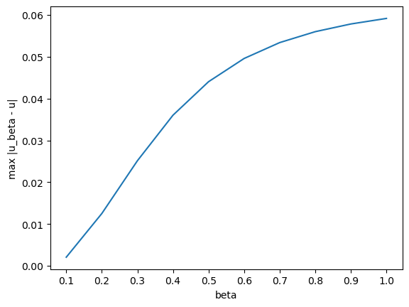
In [62], it was proved that converges at a rate of in some weighted norm. Now by regressing over , we find that the slope is using all , while the slope is using the first half . It is natural to expect that
| (6.7) |
for some . The rate (6.7) is better than the proved -rate for MFGs with a local Hamiltonian, and is between the -rate for MFGs with a general nonlocal Hamiltonian and the -rate for the example in Section 6.1. An interesting question is to find suitable conditions on model data to achieve the rate in (6.7) (with an explicit ), hence improving the bounds in [62].
7. Conclusion
This paper studies the convergence rate of the vanishing viscosity approximation to MFGs with a nonlocal, and possibly non-separable Hamiltonian. With as the diffusivity constant, we prove that and converge a rate of in the topology of uniform convergence on compact sets and the metric, respectively. Our approach exploits both probabilistic and analytical arguments, where the FBSDE representation of the MFG is used to derive the convergence rate of , and the rate of follows from a stability property of the HJB equation. We also apply our result to -player games, mean field control, and policy iteration for MFGs.
There are several directions to extend this work:
- (1)
First, our result is proved for MFGs with a nonlocal and possibly non-separable Hamiltonian. It would be interesting to establish the convergence result for MFGs with a local Hamiltonian, underpinning the numerical results in Section 6.2.
- (2)
Second, we prove in this work the convergence rate of vanishing viscosity for MFGs in ; while [59] considered the case in . The main difference between these two papers is that our work uses an FBSDE representation of the MFG together with a PDE stability result, while [59] relies exclusively on PDE arguments. A natural question is whether the FBSDE approach can be extended to other domains, so that the convergence can be established for MFGs on domains other than and .
- (3)
Finally, the vanishing viscosity approximation to MFGs can be regarded as a “perturbation” of first order MFGs, where the perturbation is to add the operator . We expect that the tools in this paper can also be used to analyze other types of perturbation, e.g., perturbation on the Hamiltonian. A notable example is the entropy-regularized relaxed control [66] in the context of reinforcement learning, where the HJB equation is replaced with the exploratory equation under entropy regularization [61].
Acknowledgment: We thank the referee for their careful reading and valuable suggestions, which have greatly improved this work. We thank Alpár Mészáros for pointing out an error in a lemma in a previous version of this work concerning the stability of McKean-Vlasov FBSDEs, and we also thank Daniel Lacker for helpful discussions on how to resolve the issue. W. Yu is supported by the Columbia Innovation Hub grant and NSF grant DMS-2309245. Q. Du is supported in part by NSF grants DMS-2309245 and DMS-1937254. W. Tang is supported by NSF CAREER Award DMS-2538791, the Tang Family Assistant Professorship and a Columbia-CityU/HK collaborative project that is supported by InnoHK Initiative, The Government of the HKSAR and the AIFT Lab.
References
- [1] (2014) Partial differential equation models in macroeconomics. Philos. Trans. R. Soc. Lond. Ser. A Math. Phys. Eng. Sci. 372 (2028), pp. 20130397, 19. Cited by: §1.1, §1.
- [2] (2020) Mean field games and applications: numerical aspects. In Mean field games, Lecture Notes in Math., Vol. 2281, pp. 249–307. Cited by: §1.
- [3] (2018) Mean field games with congestion. Ann. Inst. H. Poincaré C Anal. Non Linéaire 35 (2), pp. 443–480. Cited by: §1.1, item 4.
- [4] (2014) Continuity equations and ODE flows with non-smooth velocity. Proc. Roy. Soc. Edinburgh Sect. A 144 (6), pp. 1191–1244. Cited by: §5.2.
- [5] (2025) Global well-posedness of displacement monotone degenerate mean field games master equations. SIAM J. Control Optim. 63 (2), pp. 993–1021. Cited by: §1.1, §2.2, Remark 4.6.
- [6] (2021) A policy iteration method for mean field games. ESAIM Control Optim. Calc. Var. 27, pp. Paper No. 85, 19. Cited by: §5.3, §5.3.
- [7] (2024) A high-order scheme for mean field games. J. Comput. Appl. Math. 445, pp. Paper No. 115769, 19. Cited by: §6.1.
- [8] (2022) Rates of convergence for the policy iteration method for mean field games systems. J. Math. Anal. Appl. 512 (1), pp. Paper No. 126138, 18. Cited by: §5.3, §5.3.
- [9] (2022) A policy iteration method for mean field games. IFAC-PapersOnLine 55 (30), pp. 406–411. Cited by: §5.3, §5.3.
- [10] (2012) Notes on mean field games. Lectures by P.L. Lions at the College de France , pp. . Cited by: §2.1.
- [11] (2015) Mean field games systems of first order. ESAIM Control Optim. Calc. Var. 21 (3), pp. 690–722. Cited by: §1.1.
- [12] (2020) An introduction to mean field game theory. In Mean field games, Lecture Notes in Math., Vol. 2281, pp. 1–158. Cited by: §1.1, §2.1, footnote 3.
- [13] (2015) Weak solutions for first order mean field games with local coupling. In Analysis and geometry in control theory and its applications, Springer INdAM Ser., Vol. 11, pp. 111–158. Cited by: §1.1.
- [14] (2014) A fully discrete semi-Lagrangian scheme for a first order mean field game problem. SIAM J. Numer. Anal. 52 (1), pp. 45–67. Cited by: §1.
- [15] (2024) A Lagrange-Galerkin scheme for first order mean field game systems. SIAM J. Numer. Anal. 62 (1), pp. 167–198. Cited by: §1, §6.1.
- [16] (2018) Probabilistic theory of mean field games with applications I. Probability Theory and Stochastic Modelling, Vol. 83, Springer, Cham. Note: Mean field FBSDEs, control, and games Cited by: §1.1, §2.1.
- [17] (2015) A probabilistic weak formulation of mean field games and applications. Ann. Appl. Probab. 25 (3), pp. 1189–1231. Cited by: §1.1.
- [18] (2021) Applications of mean field games in financial engineering and economic theory. In Mean field games, Proc. Sympos. Appl. Math., Vol. 78, pp. 165–219. Cited by: §1.
- [19] (2025) Optimal rate of convergence in the vanishing viscosity for uniformly convex Hamilton-Jacobi equations. arxiv:2506.13255. Cited by: §1.1.
- [20] (2025) Convergence rates for the vanishing viscosity approximation of Hamilton-Jacobi equations: the convex case. arxiv:2502.15495. Cited by: §1.1.
- [21] (2024) Long time behavior and stabilization for displacement monotone mean field games. arXiv:2412.14903. Cited by: §6.1.
- [22] (2021) On the role of numerical viscosity in the study of the local limit of nonlocal conservation laws. ESAIM Math. Model. Numer. Anal. 55 (6), pp. 2705–2723. Cited by: footnote 2.
- [23] (2019) On the singular local limit for conservation laws with nonlocal fluxes. Arch. Ration. Mech. Anal. 233 (3), pp. 1131–1167. Cited by: footnote 2.
- [24] (1983) Viscosity solutions of Hamilton-Jacobi equations. Trans. Amer. Math. Soc. 277 (1), pp. 1–42. Cited by: §1.
- [25] (2024) On the optimal rate for the convergence problem in mean field control. J. Funct. Anal. 287 (12), pp. Paper No. 110660, 94. Cited by: §5.2, §5.2, §5.2.
- [26] (2019) From the master equation to mean field game limit theory: a central limit theorem. Electron. J. Probab. 24, pp. 1–54. Cited by: §5.1.
- [27] (2020) From the master equation to mean field game limit: large deviations and concentration of measure. Ann. Probab. 48 (1), pp. 211–263. Cited by: §5.1, §5.1, §5.1, §5.1, Corollary 5.1.
- [28] (2017) Mean-field-type games in engineering. AIMS Electronics and Electrical Engineering 1 (1), pp. 18–73. Cited by: §1.
- [29] (2022) Extended mean field control problem: a propagation of chaos result. Electron. J. Probab. 27 (), pp. 1–53. External Links: Link Cited by: §5.1.
- [30] (2020) The CLT in high dimensions: quantitative bounds via martingale embedding. Ann. Probab. 48 (5), pp. 2494–2524. Cited by: §5.2.
- [31] (2021) Existence of weak solutions to time-dependent mean-field games. Nonlinear Anal. 212, pp. Paper No. 112470, 31. Cited by: §1.1.
- [32] (2022) On the connection between symmetric n-player games and mean field games. Ann. Appl. Probab. 27 (2), pp. 757–810. External Links: Link Cited by: §5.1.
- [33] (2019) On differentiability in the Wasserstein space and well-posedness for Hamilton-Jacobi equations. J. Math. Pures Appl. 9, pp. 119–174. Cited by: §2.1.
- [34] (2022) Mean field games master equations with nonseparable Hamiltonians and displacement monotonicity. Ann. Probab. 50 (6), pp. 2178–2217. Cited by: §1.1.
- [35] (2025) Non-separable mean field games for pedestrian flow: generalized Hughes model. Math. Models Methods Appl. Sci. 35 (7), pp. 1571–1607. Cited by: §1.
- [36] (1984) A class of Wasserstein metrics for probability distributions. Michigan Math. J. 31, pp. 231 – 240. Cited by: §5.2.
- [37] (2023) On monotonicity conditions for mean field games. J. Funct. Anal. 285 (9), pp. Paper No. 110095, 45. Cited by: §2.2, Remark 2.8.
- [38] (2025) Policy iteration for nonconvex viscous Hamilton–Jacobi equations. arXiv:2503.02159. Cited by: §5.3.
- [39] (2020) A game-theoretic framework for autonomous vehicles velocity control: bridging microscopic differential games and macroscopic mean field games. Discrete Contin. Dyn. Syst. Ser.B 25 (12), pp. 4869–4903. Cited by: §1.
- [40] (2007) Large-population cost-coupled LQG problems with nonuniform agents: individual-mass behavior and decentralized -Nash equilibria. IEEE Trans. Automat. Control 52 (9), pp. 1560–1571. Cited by: §1.
- [41] (2006) Large population stochastic dynamic games: closed-loop Mckean-Vlasov systems and the nash certainty equivalence principle. Commun. Inf. Syst. 6 (3), pp. 221–252. Cited by: §1.
- [42] (2020) Exponential convergence and stability of Howard’s policy improvement algorithm for controlled diffusions. SIAM J. Control Optim. 58 (3), pp. 1314–1340. Cited by: §5.3.
- [43] (2015) Mean field games via controlled martingale problems: existence of Markovian equilibria. Stochastic Process. Appl. 125 (7), pp. 2856–2894. Cited by: §1.1.
- [44] (2020) On the convergence of closed-loop nash equilibria to the mean field game limit. Ann. Appl. Probab. 30 (4), pp. 1693–1761. External Links: Link Cited by: §5.1.
- [45] (2006) Jeux à champ moyen. I. le cas stationnaire. C. R. Math. Acad. Sci. Paris 343 (9), pp. 619–625. Cited by: §1.
- [46] (2006) Jeux à champ moyen. II – horizon fini et contrôle optimal. C. R. Math. Acad. Sci. Paris 343 (10), pp. 679–684. Cited by: §1.
- [47] (2007) Mean field games. Jpn. J. Math. 2 (1), pp. 229–260. Cited by: §1.
- [48] (2023) Policy iteration method for time-dependent mean field games systems with non-separable Hamiltonians. Appl. Math. Optim. 87 (17). External Links: Link Cited by: §5.3, §5.3.
- [49] (2001) -Stability and error estimates for approximate Hamilton-Jacobi solutions. Numer. Math. 87 (4), pp. 701–735. Cited by: §1.1, Remark 2.8.
- [50] (2021) Computational methods for first-order nonlocal mean field games with applications. SIAM J. Numer. Anal. 59 (5), pp. 2639–2668. Cited by: §1.
- [51] (2024) Convergence analysis for entropy-regularized control problems: a probabilistic approach. arXiv:2406.10959. Cited by: §5.3.
- [52] (2024) Mean field games systems under displacement monotonicity. SIAM J. Math. Anal. 56 (1), pp. 529–553. Cited by: §1.1, §2.2, §2.3, Assumption 2.1, Assumption 2.2, Assumption 2.3, Assumption 2.5, Definition 2.9, §3, §3.
- [53] (2019) Mean field games in macroeconomics. Econ Meets Math Workshop. Note: Available at https://benjaminmoll.com/wp-content/uploads/2020/10/MFG_macro.pdf Cited by: §1.1, §1.
- [54] (2024) Mean field game master equations with anti-monotonicity conditions. arXiv:2201.10762. To appear in J. Eur. Math. Soc.. Cited by: §2.2.
- [55] (2014) A probability path. First edition, Modern Birkhäuser Classics, Birkhäuser Boston, MA. External Links: ISBN 978-0-8176-8408-2 Cited by: §3.
- [56] (2009) Upper bounds for minimal distances in the central limit theorem. Ann. Inst. Henri Poincaré Probab. Stat. 45 (3), pp. 802–817. Cited by: footnote 7.
- [57] (1985) Existence of viscosity solutions of Hamilton-Jacobi equations. J. Differential Equations 56 (5), pp. 345–390. Cited by: footnote 5.
- [58] (1984) Numerical viscosity and the entropy condition for conservative difference schemes. Math. Comp. 43 (168), pp. 369–381. Cited by: footnote 2.
- [59] (2023) The Poisson binomial distribution—old & new. Statist. Sci. 38 (1), pp. 108–119. Cited by: item 2, footnote 7.
- [60] (2025) Policy iteration for the deterministic control problems—a viscosity approach. SIAM J. Control Optim. 63 (1), pp. 375–401. Cited by: §5.3, footnote 10.
- [61] (2022) Exploratory HJB equations and their convergence. SIAM J. Control Optim. 60 (6), pp. 3191–3216. Cited by: item 3.
- [62] (2025) The convergence rate of vanishing viscosity approximations for mean field games. SIAM J. Math. Anal. 57 (3), pp. 3217–3254. Cited by: §1.1, §1, §2.3, Remark 2.8, Remark 2.8, Remark 2.8, §4, §4, §6.2, §6.2, footnote 5.
- [63] (2024) Regret of exploratory policy improvement and -learning. arXiv:2411.01302. Cited by: §5.3.
- [64] (2024) Trading and wealth evolution in the proof of stake protocol. In Proof-of-Stake for Blockchain Networks: Fundamentals, Challenges and Approaches, pp. 135–161. External Links: Link Cited by: §1.1, §1, item 3.
- [65] (2025) Policy iteration for exploratory Hamilton–Jacobi–Bellman equations. Appl. Math. Optim. 91 (2), pp. Paper No. 50. Cited by: §5.3.
- [66] (2020) Reinforcement learning in continuous time and space: a stochastic control approach. J. Mach. Learn. Res. 21, pp. 1–34. Cited by: item 3.
- [67] (2017) An elementary proof for the structure of Wasserstein derivatives. Note: arXiv:1705.08046 Cited by: §2.1.
- [68] (2018) A high-dimensional CLT in distance with near optimal convergence rate. Probab. Theory Related Fields 170 (3-4), pp. 821–845. Cited by: footnote 9.