Focus on What Matters: Enhancing Medical Vision-Language Models with Automatic Attention Alignment Tuning
Abstract
Medical Large Vision-Language Models (Med-LVLMs) often exhibit suboptimal attention distribution on visual inputs, leading to hallucinated or inaccurate outputs. Existing mitigation methods primarily rely on inference-time interventions, which are limited in attention adaptation or require additional supervision. To address this, we propose A3Tune, a novel fine-tuning framework for Automatic Attention Alignment Tuning. A3Tune leverages zero-shot weak labels from SAM, refines them into prompt-aware labels using BioMedCLIP, and then selectively modifies visually-critical attention heads to improve alignment while minimizing interference. Additionally, we introduce a A3MoE module, enabling adaptive parameter selection for attention tuning across diverse prompts and images. Extensive experiments on medical VQA and report generation benchmarks show that A3Tune outperforms state-of-the-art baselines, achieving enhanced attention distributions and performance in Med-LVLMs.11 1 Source code is available at https://github.com/Aofei-Chang/A3Tune
1 Introduction

While medical Large Vision-Language Models (Med-LVLMs) have shown significant progress in the medical domain Li et al. (2024); Chen et al. (2024d); Thawkar et al. (2023); Moor et al. (2023), they often produce inaccurate or hallucinated outputs that deviate from the provided visual medical information, as revealed by recent benchmarks Xia et al. (2024); Gu et al. (2024); Chen et al. (2024a). An example of medical visual question answering (VQA) extracted from the SLAKE Liu et al. (2021) dataset is shown in Figure 1(A), where we visualize the average attention map on the image inputs during generating answers. We can observe that LLaVA-Med in Figure 1(A.2) generates the hallucinated response “Alzheimer’s disease”, neglecting the tumor region and over-focusing on irrelevant background areas, as shown in the corresponding attention map. This reveals a significant bias in attention distribution on visual inputs that limits the model’s effectiveness, which have been identified in general LVLMs Gong et al. (2024); Woo et al. (2024); Liu et al. (2025).
Unfortunately, none of the specified bias mitigation strategies have been proposed in the medical domain. In the general domain, research primarily focuses on inference-time interventions to reduce attention biases, employing two main approaches. The first approach, contrastive decoding Leng et al. (2024); Favero et al. (2024); Liu et al. (2025); Woo et al. (2024); Gong et al. (2024), introduces a contrastive adjustment to the decoding logits. However, this method does not directly modify the attention distribution, meaning it cannot guarantee that the model attends to diagnostically critical regions. The second approach directly modifies attention maps during inference, as seen in ControlMLLM Wu et al. (2024), which enforces the model to focus on pre-annotated regions of interest (RoIs). However, as shown in Figure1(A.3), this method still generates partially hallucinated content. Besides, it requires additional tuning and ground truth RoIs for each inference process, making it impractical for real-world applications.
To overcome the limitations of inference-time intervention, an ideal solution is to automatically adjust attention maps towards RoIs during fine-tuning for downstream medical tasks. This approach enables the model to place more attention on critical regions during inference, eliminating the need for additional labels or interventions. However, implementing such a method poses several challenges:
(1) Limited availability of medical segmentation labels. As shown in Figure 1(A.3), using segmentation labels (RoIs) as guidance, as done in ControlMLLM, can enhance the learning of accurate attention maps and answer correctness. However, such labels are often unavailable in medical datasets.
(2) Trade-off between attention alignment and model stability. Assuming that RoI labels are available, directly modifying the attention maps of all attention heads towards the labels without any strategy is still risky. This may lead to the over-alignment issue that potentially impacts the output stability and overall performance. Therefore, achieving the right balance between attention alignment and model stability is essential.
(3) Adapting attention to diverse prompts and images. Even if attention alignment and model stability are balanced, the parameter-sharing strategy in fine-tuning remains a limitation for adaptive attention alignment. For example, as shown in Figure 1, the optimal RoIs can vary significantly based on the input prompt and image, requiring dynamic alignment. While the computation of attention maps adjusts to input representations, the shared parameters in fine-tuning limit the model’s ability to flexibly learn attention distribution across diverse inputs.

To address these challenges simultaneously, we propose A3Tune, a novel fine-tuning framework designed for Automatic Attention Alignment Tuning. As shown in Figure 2, A3Tune integrates a set of cooperative strategies to ensure that attention in Med-LVLMs is well aligned, minimally disruptive, and highly adaptable across diverse medical tasks. Firstly, to overcome the lack of segmentation labels (Challenge 1), A3Tune utilizes zero-shot segmentation labels generated by SAM Roy et al. (2023) and further refines them into prompt-aware weak labels using BioMedCLIP Zhang et al. (2023). These weak labels serve as guidance for attention alignment, eliminating the need for manual annotations. However, weak labels alone are not sufficient — uncontrolled modifications on all attention heads can disrupt model stability (Challenge 2). To further balance attention alignment with model stability, A3Tune selectively modifies only the most “visually-critical” attention heads, minimizing the risk of over-alignment and instability. Furthermore, the parameter-sharing strategy in alignment tuning remains a limitation, as RoIs vary significantly based on the input prompt and image (Challenge 3). To address this, we incorporate a custom-designed Mixture-of-Experts A3MoE into A3Tune on attention modules, allowing the model to dynamically select parameters and adjust attention maps for different images and prompts.
In summary, this work makes the following contributions: (1) We propose A3Tune, a novel visual attention tuning approach that utilizes zero-shot weak labels to refine the visual focus of Med-LVLMs and enhance their performance. (2) We develop a set of designs for cooperative attention alignment tuning: (i) weak label supervision, (ii) selective tuning of visually-critical attention heads, and (iii) a A3MoE module for adaptive attention adjustment. (3) We conduct extensive experiments on five medical VQA and two report generation benchmarks against ten baselines, demonstrating that A3Tune outperforms state-of-the-art methods in both effectiveness and interpretability, improving visual grounding and overall model performance.
2 Related Work
While some efforts, such as CoMT Jiang et al. (2024), have attempted to reduce hallucinations in Med-LVLMs for report generation by training on hierarchical QA pairs derived from real clinical image reports, mitigation strategies specifically designed for Med-LVLMs remain largely underexplored. Since Med-LVLMs share the same structure and training process as general LVLMs, hallucination issues are a common challenge across both. As a result, many inference-time mitigation strategies developed for LVLMs are also applicable to Med-LVLMs, including: (1) Enhancing visual information and mitigating text over-reliance: VCD Leng et al. (2024), M3ID Favero et al. (2024), PAI Liu et al. (2025), HELPD Yuan et al. (2024), RBD Liang et al. (2024). (2) Mitigating visual token attention bias, with approaches such as AVISC Woo et al. (2024) and DAMRO Gong et al. (2024). (3) Refining and modifying LLM generation patterns during decoding, OPERA Huang et al. (2024), DoLa Chuang et al. (2023). In addition, other mitigation methods, such as TruthFlow Wang et al. (2025), leverage trained steering vectors to guide the model toward more truthful outputs in LLMs. Despite these advancements, significant challenges remain in mitigation attention biases in Med-LVLMs.
3 Preliminaries
3.1 Background of Med-LVLMs
Med-LVLMs share the same fundamental architecture as general LVLMs Liu et al. (2024); Chen et al. (2023), consisting of three primary components: the Visual Encoder, the Visual Alignment Layer, and the Large Language Model (LLM). The input image is firstly divided into patches and processed by the Visual Encoder, which converts it into a sequence of visual tokens with embeddings represented as , where denotes the dimension of the visual hidden representation.
The visual tokens are then projected through the Visual Alignment Layer into , where denotes the dimension of the LLM token space. These aligned visual tokens are subsequently forwarded to the LLM along with the embeddings of the tokenized textual prompts , where is the number of text tokens.
The final objective of the LLM in Med-LVLMs is to predict the next token based on the current visual input , prompt input , and previously generated tokens , formulated as:
| (1) |
where denotes the parameters of the LLM.
3.2 Visual Attention Map
Most Med-LVLMs adopt a Transformer Vaswani et al. (2017) decoder-based LLM, which processes inputs through decoder layers, each equipped with a multi-head attention module. In layer , the module includes attention heads, where each head (with ) computes attention separately using their corresponding attention map . This attention mechanism models relationships between visual and textual tokens.
To analyze how visual tokens contribute to text generation, we focus on the attention scores between visual tokens and subsequent text tokens, referred to as visual attention map , a submatrix of the overall attention map . To gain a global understanding of attention distribution on visual tokens, the averaged visual attention map can be obtained by aggregating attention across all heads and layers Wu et al. (2024):
| (2) |
4 The Proposed A3Tune
A3Tune aims to automatically align attention to enhance visual grounding and improve the performance of Med-LVLMs. The fine-tuning pipeline is illustrated in Figure 2. Given an input image and prompt , we firstly generate a set of prompt-aware weak labels using a zero-shot method (Section 4.1). To achieve effective attention alignment (Section 4.2) with the guidance of , we first identify visually-critical attention heads, then integrate an A3MoE design into each decoder layer to enable flexible attention distribution learning.
4.1 Prompt-Aware Weak Labels Generation
Given a medical image , we first use SAM Kirillov et al. (2023) to generate a set of candidate segments following Yang et al. (2024). However, using all segments in for attention tuning introduces noise, as only a subset is relevant to each prompt. Therefore, it is necessary to select prompt-aware segments as weak labels to adaptively guide attention tuning. To filter prompt-aware weak labels, we embed each segment into a feature representation using BioMedCLIP’s vision encoder, while the text prompt is embedded into using its text encoder. We then select an adaptive threshold to select segments that are most similar to the text prompt based on cosine similarity (Sim) in the embedding space:
| (3) |
4.2 Visual Attention Alignment Tuning
The goal of visual attention alignment tuning is to align averaged visual attention map with fixed weak labels (i.e., masking regions) via Eq. (3) during fine-tuning. To achieve this goal, we first design a new parameter-efficient fine-tuning strategy and select “visually-critical” attention heads to the alignment of attention maps with .
4.2.1 A3MoE Design
We build A3Tune based on a parameter-efficient fine-tuning technique, LoRA Hu et al. (2021), and apply it to all linear modules of the LLM in the Med-LVLM, including the Query and Key matrices in attention modules. In standard LoRA fine-tuning, the trainable LoRA parameters and for Query and Key matrices are shared across all training instances. However, this static parameter-sharing strategy in attention is insufficient for A3Tune. As shown in the abdominal organ analysis tasks (Figure 3), weak labels vary with the prompt, yet attention maps generated with shared and lack the flexibility to adapt effectively to different prompts and images.
To address this limitation, we introduce A3MoE, a Mixture-of-Experts mechanism specifically designed for A3Tune, with two sub-modules: Q-MoE and K-MoE, applied to the LoRA parameters and in each LLM decoder layer . For clarity, we omit the explicit annotation of in subsequent equations, as A3MoE is applied consistently across all decoder layers. The following sections describe these sub-modules in detail.

Q-MoE: Prompt-Level MoE on Query Matrix. As shown in Figure 3, the target RoIs often depend on the text prompt, even for the same image. To handle this, we introduce Q-MoE, a prompt-level MoE on , consisting of experts. For the -th expert (), we define , where and are matrices with a low rank .
To dynamically route experts based on the prompt, we apply a prompt-level gating mechanism that generates router weights based on the hidden states of the prompt , which is obtained at each layer after processing from the previous decoder layers. To capture the prompt’s overall context, is first averaged using a pooling operation. The routing and parameter computation are formulated as:
| (4) | |||
| (5) |
where represents the router weights, with each determining the contribution of the corresponding expert . MLP denotes the multi-layer perceptron used in the gating mechanism.
K-MoE: Visual Token-Level Sparse MoE in Key Matrix. Unlike text prompts, which can be summarized with pooling, visual inputs contain fine-grained information at the token level, where subtle differences can indicate abnormalities that require varied attention. To capture these nuances, we introduce K-MoE, a visual token-level MoE applied on . K-MoE includes experts, each implemented using LoRA.
For each visual token , the gating mechanism dynamically select experts based on its hidden states , and the LoRA parameters for visual token are computed as:
| (6) | |||
| (7) |
where and is a binary indicator enforcing sparsity by retaining only the top- gating weights. It is set to if expert is among the top- most relevant experts, otherwise it is set to . This mechanism ensures that for each visual token, only the most relevant experts contribute, minimizing interference among visual tokens while improving efficiency in alignment tuning.
4.2.2 “Visually-Critical” Heads Selection
Each layer in the LLM decoder fine-tuned with A3MoE learns attention heads and the total number of attention heads is . Among them, the attention heads that assign higher weights to visual information are more crucial in processing visual features. Thus in layer , the importance of each head can be quantified using the visual attention ratio , which measures the proportion of attention allocated to visual tokens relative to all tokens as follows:
| (8) |
where represents the attention score assigned by attention head in layer to token .
To refine the visual attention matrix , we select top- “visually-critical” heads based on the visual attention ratios . To achieve this, we use a binary indicator to identify and retain only the most influential attention heads. Specifically, it is set to if attention head is among the heads with the highest visual attention ratios and otherwise. The updated visual attention matrix is then computed as:
| (9) |
4.2.3 Attention Alignment Function
After obtaining refined , we define how it is adjusted to align with the weak labels . Intuitively, in the averaged attention map , tokens within the masking regions should receive higher attention values. Motivated by the cross-attention control design for image generation in Chen et al. (2024c), we use a mask-based energy function to guide the attention alignment tuning:
| (10) |
where represents each referring segment in , and is the visual token index, and is the number of visual tokens. Among all visual tokens, this function encourages higher attention on visual tokens within each , minimizing the loss and guiding to effectively focus on the prompt-aware regions .
| Model | Method | Slake | VQA-RAD | PathVQA | IU-Xray | OmniVQA | |||
| Open | Closed | Open | Closed | Open | Closed | Closed | Closed | ||
| LLaVA-Med | LLaVA-Med | 41.28 | 57.75 | 32.48 | 68.90 | 10.34 | 52.49 | 72.83 | 31.79 |
| Greedy | 42.81 | 60.00 | 35.68 | 68.11 | 11.35 | 52.34 | 75.00 | 31.11 | |
| Beam Sutskever et al. (2014) | 42.31 | 61.69 | 33.57 | 66.93 | 9.86 | 53.79 | 73.59 | 30.89 | |
| Nucleus Holtzman et al. (2020) | 41.06 | 61.41 | 32.64 | 68.11 | 9.93 | 53.17 | 73.09 | 30.96 | |
| VCD Leng et al. (2024) | 39.76 | 59.44 | 33.93 | 66.54 | 11.17 | 53.52 | 74.36 | 32.89 | |
| DoLa Chuang et al. (2023) | 42.37 | 59.72 | 35.68 | 68.50 | 11.38 | 52.55 | 74.87 | 31.04 | |
| OPERA Huang et al. (2024) | 40.44 | 60.00 | 35.54 | 68.50 | 9.77 | 53.17 | 75.00 | 31.72 | |
| AVISC Woo et al. (2024) | 41.46 | 59.72 | 35.43 | 64.17 | 11.03 | 52.20 | 73.85 | 32.48 | |
| M3ID Favero et al. (2024) | 38.85 | 60.28 | 35.31 | 62.60 | 9.80 | 52.93 | 72.32 | 31.11 | |
| DAMRO Gong et al. (2024) | 41.33 | 59.72 | 32.73 | 66.54 | 10.80 | 51.84 | 72.19 | 31.45 | |
| PAI Liu et al. (2025) | 43.18 | 60.28 | 35.10 | 68.50 | 11.09 | 52.46 | 74.87 | 32.13 | |
| LLaVA-Med + LoRA | LLaVA-Med + LoRA | 80.65 | 82.82 | 33.37 | 66.54 | 31.92 | 90.95 | 83.29 | 90.65 |
| Greedy | 81.12 | 85.07 | 31.88 | 68.50 | 33.90 | 91.86 | 83.93 | 90.73 | |
| Beam Sutskever et al. (2014) | 81.32 | 86.76 | 32.55 | 68.90 | 33.60 | 91.92 | 84.06 | 90.58 | |
| Nucleus Holtzman et al. (2020) | 80.18 | 85.35 | 31.34 | 68.50 | 30.14 | 90.92 | 83.41 | 90.05 | |
| VCD Leng et al. (2024) | 79.58 | 84.23 | 32.96 | 67.72 | 30.20 | 90.86 | 83.93 | 90.73 | |
| DoLa Chuang et al. (2023) | 81.84 | 86.48 | 31.94 | 68.50 | 34.00 | 91.86 | 84.06 | 90.69 | |
| OPERA Huang et al. (2024) | 81.25 | 86.48 | 33.18 | 68.90 | 33.64 | 91.80 | 84.06 | 90.42 | |
| AVISC Woo et al. (2024) | 80.15 | 85.63 | 33.66 | 69.29 | 32.37 | 90.62 | 84.06 | 90.54 | |
| M3ID Favero et al. (2024) | 79.83 | 84.79 | 31.40 | 68.90 | 32.47 | 91.15 | 84.95 | 90.73 | |
| DAMRO Gong et al. (2024) | 82.19 | 83.66 | 32.41 | 66.14 | 32.27 | 90.12 | 84.69 | 90.08 | |
| PAI Liu et al. (2025) | 81.02 | 86.76 | 32.14 | 68.11 | 33.46 | 91.77 | 84.31 | 90.95 | |
| A3Tune (ours) | 82.36 | 86.76 | 36.97 | 70.87 | 34.61 | 92.19 | 85.97 | 91.98 | |
4.3 Final Objective
In the fine-tuning process, we incorporate the loss of proposed visual attention alignment tuning (Eq. 10) as a regularization term for downstream medical tasks. This term is combined with the language modeling objective :
| (11) |
where denotes the frozen parameters of LLM, denotes the trainable parameters in LoRA and A3MoE, and denotes the generated tokens before time step . The final objective loss is:
| (12) |
where is a hyperparameter that controls the strength of attention tuning.
5 Experiments
We evaluate our method on representative Med-LVLMs, including LLaVA-Med Li et al. (2024) and LLaVA-Med-1.5. The experimental results for LLaVA-Med-1.5 are provided in Appendix G.
5.1 Settings
Datasets. We evaluate our method on two key tasks in medical application of Med-LVLMs: medical VQA and medical report generation. For medical VQA, we use diverse datasets including SLAKE Liu et al. (2021), VQA-RAD Lau et al. (2018), PathVQA He et al. (2020), IU-Xray Demner-Fushman et al. (2016) and OmniMedVQA Hu et al. (2024). For medical report generation, we use MIMIC-CXR Johnson et al. (2019) and IU-Xray. Details of dataset processing and settings are provided in Appendix A.
Baselines. We compare our approach with widely used hallucination mitigation methods with or without fine-tuning, including decoding strategies and contrastive decoding techniques22 2 We do not compare with the methods requiring tailored de-hallucination training pipelines such as CoMT Jiang et al. (2024) and HELPD Yuan et al. (2024). . The decoding baselines include Greedy decoding, Nucleus sampling Holtzman et al. (2020), Beam search Sutskever et al. (2014). For contrastive decoding techniques, we specifically compare with: VCD Leng et al. (2024), OPERA Huang et al. (2024), DoLa Chuang et al. (2023), AVISC Woo et al. (2024), M3ID Favero et al. (2024), DAMRO Gong et al. (2024) and PAI Liu et al. (2025). Additionally, we include ControlMLLM Wu et al. (2024) as a baseline only when the ground truth RoIs are available. Detailed settings of baselines and implementation are in Appendix B and Appendix C, respectively.
| Method | Metrics | |
| Coverage | Intensity | |
| LLaVA-Med | 0.122 | 0.076 |
| LLaVA-Med + LoRA | 0.132 | 0.076 |
| A3Tune | 0.275 | 0.147 |
| Dataset | Metric | Method | |||||||||||
| LLaVA-Med + LoRA | Greedy | Beam | Nucleus | VCD | DoLa | OPERA | AVISC | M3ID | DAMRO | PAI | A3Tune | ||
| IU-Xray | BLEU | 7.70 | 8.86 | 9.34 | 7.80 | 8.83 | 8.93 | 8.27 | 8.52 | 8.63 | 7.29 | 8.87 | 11.05 |
| ROUGE-L | 26.15 | 27.09 | 27.56 | 26.72 | 27.36 | 26.94 | 27.14 | 26.97 | 27.79 | 25.61 | 26.74 | 30.00 | |
| METEOR | 29.50 | 26.01 | 26.44 | 30.33 | 31.77 | 25.74 | 29.66 | 31.14 | 31.65 | 30.03 | 25.99 | 34.26 | |
| BERTScore | 88.36 | 88.50 | 88.52 | 88.28 | 88.30 | 88.42 | 88.41 | 88.47 | 88.52 | 88.14 | 88.39 | 89.05 | |
| CheXbert | 53.81 | 52.55 | 52.88 | 52.73 | 51.86 | 52.27 | 56.26 | 53.33 | 54.45 | 51.50 | 52.45 | 57.19 | |
| RadGraph | 20.44 | 20.76 | 21.29 | 20.85 | 22.02 | 20.63 | 21.87 | 22.27 | 22.22 | 20.75 | 20.48 | 24.24 | |
| RaTEScore | 58.37 | 58.24 | 58.77 | 57.84 | 58.93 | 58.10 | 58.73 | 59.21 | 59.37 | 59.19 | 57.81 | 63.03 | |
| MIMIC- CXR | BLEU | 3.28 | 4.07 | 3.39 | 3.29 | 3.53 | 3.99 | 3.14 | 3.34 | 3.62 | 3.37 | 4.32 | 4.56 |
| ROUGE-L | 16.54 | 18.75 | 17.25 | 16.14 | 16.58 | 18.62 | 15.52 | 16.79 | 16.67 | 15.75 | 18.64 | 19.03 | |
| METEOR | 17.90 | 18.81 | 17.36 | 17.98 | 18.68 | 18.68 | 14.70 | 18.29 | 18.22 | 17.03 | 19.78 | 20.23 | |
| BERTScore | 85.57 | 86.14 | 85.78 | 85.42 | 85.57 | 86.14 | 84.75 | 85.59 | 85.58 | 85.27 | 86.10 | 86.17 | |
| CheXbert | 22.14 | 24.24 | 23.05 | 21.76 | 23.38 | 25.14 | 20.07 | 22.74 | 22.95 | 22.76 | 25.78 | 24.93 | |
| RadGraph | 9.43 | 10.73 | 9.78 | 9.20 | 9.93 | 10.75 | 7.74 | 9.52 | 9.93 | 9.40 | 11.17 | 11.55 | |
| RaTEScore | 40.00 | 41.06 | 38.59 | 39.26 | 40.95 | 40.73 | 35.72 | 40.08 | 39.87 | 39.62 | 41.03 | 42.73 | |
Metrics. (1) Metrics for Performance Evaluation. For medical VQA, we report Accuracy for close-ended questions and Recall for open-ended questions, following LLaVA-Med Li et al. (2024). For medical report generation, we use standard metrics for generation tasks, including BLEU Papineni et al. (2002), ROUGE-L Lin (2004), METEOR Banerjee and Lavie (2005), and BERTScore Zhang et al. (2019). Additionally, we report domain-specific metrics designed for medical report generation: CheXbert Smit et al. (2020), RadGraph Jain et al. (2021) and RaTEScore Zhao et al. (2024). More details of these metrics are provided in Appendix D.1. (2) Metrics for Attention Maps Evaluation. For datasets with ground truth RoIs (e.g., SLAKE), we design two metrics to evaluate the attention distribution on images: (1) Coverage Score (Coverage), which measures spatial alignment, and (2) Intensity Alignment (Intensity), which assesses the degree of focus. Details of these two metrics are in Appendix D.2.
5.2 Medical VQA Results
The performance of A3Tune on diverse medical VQA benchmarks is presented in Table 1, indicating A3Tune maintains its superiority across all datasets and its effectiveness across diverse medical images and VQA tasks. In addition, we also analyze visual attention distribution on the test set of SLAKE with annotated RoIs (Table 2). Since the baselines in Table 1 improve the model only on the decoding side without modifying attentions, their attention distributions remain similar to the base model, LLaVA-Med and we compare only against LLaVA-Med and LLaVA-Med + LoRA. We observe that A3Tune achieves the highest scores in both coverage (0.275) and intensity (0.147), outperforming baselines. These results highlight A3Tune’s ability to focus more effectively on RoIs in medical images, explaining its better VQA performance and improved interpretability.
5.3 Medical Report Generation Results
Table 3 presents the evaluation of A3Tune on medical report generation tasks using traditional metrics (e.g., BLEU, ROUGE-L) and domain-specific metrics such as RaTEScore. The baselines are applied on fine-tuned LLaVA-Med using LoRA, as the original LLaVA-Med performs significantly worse on this task, as shown in the full results in Appendix E. Similar to the results in Table 1, A3Tune outperforms all baselines across both datasets and almost all metrics.
5.4 Module Effectiveness Analysis
5.4.1 Weak Labels Generation
(1) Quality of Weak Labels. This experiment evaluates the upper bound of A3Tune’s performance by upgrading weak labels to high-quality ground truth labels (GT). We use a subset of SLAKE with RoIs annotations, including 992 training samples and 206 test samples and take ControlMLLM Wu et al. (2024) as the baseline.
Figure 4 (B.2) shows that replacing weak labels (Weak) with high-quality labels (GT in A3Tune further improves performance, validating the reasonableness of using weak labels. Additionally, while ControlMLLM (Control) improves performance in LLaVA-Med (Figure 4 (A)), it negatively impacts fine-tuned LLaVA-Med+LoRA in Figure 4 (B.1), whereas A3Tune achieve improved results. These results highlight both the effectiveness of A3Tune and its potential for further improvement when ground truth RoI labels are available.


(2) Selection of Weak Labels. To obtain prompt-aware weak labels, we select segments that are most similar to the text prompt. In this experiment, we analyze the impact of different values of on model performance using the SLAKE dataset. As shown in Figure 5 (a) increasing initially improves performance by adding more relevant labels. However, performance peaks at , after which additional segments introduce noise, leading to a performance decline.
5.4.2 Selection of Attention Heads
In A3Tune, we select most “visually-critical” attention heads to balance model stability and effectiveness of A3Tune. As shown in Figure 5 (b), disabling attention tuning () results in noticeably lower performance. Performance peaks at , which strikes a balance between the strength of attention tuning and stability. Thus, we set in our experiments.
5.4.3 A3MoE Design
| Model | Metric | Method | |||||||||||
| Base | Greedy | Beam | Nucleus | VCD | DoLa | OPERA | AVISC | M3ID | DAMRO | PAI | A3Tune | ||
| HuatuoGPT-V + LoRA | Open-ended | 85.46 | 84.89 | 85.62 | 85.57 | 85.57 | 85.19 | 85.07 | 84.42 | 85.41 | 85.57 | 83.85 | 86.77 |
| Close-ended | 91.27 | 89.86 | 89.86 | 90.99 | 90.99 | 90.42 | 89.86 | 90.70 | 91.27 | 90.99 | 90.99 | 91.55 | |
| Dataset | Metric | Method | |||||||||||
| HuatuoGPT-V + LoRA | Greedy | Beam | Nucleus | VCD | DoLa | OPERA | AVISC | M3ID | DAMRO | PAI | A3Tune | ||
| IU-Xray | BLEU | 8.65 | 9.34 | 10.21 | 8.19 | 9.10 | 9.03 | 10.01 | 7.47 | 8.35 | 9.10 | 6.92 | 10.52 |
| ROUGE-L | 27.34 | 28.17 | 28.64 | 26.28 | 27.80 | 27.50 | 28.57 | 24.78 | 27.05 | 27.80 | 24.36 | 28.85 | |
| METEOR | 31.48 | 31.76 | 34.23 | 30.72 | 32.13 | 31.24 | 34.10 | 30.88 | 32.17 | 32.13 | 30.84 | 36.30 | |
| BERTScore | 88.35 | 88.53 | 88.60 | 88.19 | 88.36 | 88.39 | 88.51 | 87.77 | 88.19 | 88.36 | 87.44 | 88.67 | |
| CheXbert | 54.21 | 55.16 | 55.84 | 53.86 | 54.34 | 53.89 | 55.01 | 52.11 | 53.78 | 54.34 | 50.09 | 56.27 | |
| RadGraph | 21.35 | 21.86 | 22.47 | 20.17 | 21.65 | 21.04 | 22.59 | 19.71 | 21.19 | 21.65 | 18.26 | 23.51 | |
| RaTEScore | 58.21 | 58.66 | 59.78 | 58.29 | 58.29 | 57.84 | 59.33 | 56.49 | 57.86 | 58.29 | 55.16 | 60.51 | |
(1) Ablation Study of A3MoE. Figure 7 (a) shows the impact of removing key components of A3MoE from A3Tune: Q-MoE, K-MoE and A3MoE as a whole. The removal of each module leads to a noticeable performance drop, particularly for K-MoE. This highlights the importance of K-MoE, which is designed for fine-grained attention tuning at the visual token level and is critical for datasets with diverse image modalities like SLAKE. Additionally, the removal of the entire A3MoE leads to a further decline in performance. However, even with these components removed, the performance of A3Tune remains above the baseline LoRA tuning on LLaVA-Med, demonstrating the effectiveness of the overall framework.
(2) The Number of Selected Experts in K-MoE. As shown in Figure 7(b), performance peaks at . Beyond this point, additional experts lead to diminishing and unstable returns, likely due to saturation and increased interference among experts handling different visual tokens.
5.5 Case Study
Figure 6 presents a case study for three image modalities. The attention map visualizations demonstrate that our method effectively redirects the model’s focus to relevant regions, mitigating hallucination issues compared to baselines. In addition, we provide fine-grained effectiveness evaluation across Chest X-ray, Abdomen CT, and Brain MRI images from SLAKE in Appendix F Table 10.
5.6 Generalization to Other Medical LVLMs
We further evaluate our approach on medical VQA (Table 4) and report generation (Table 5) using a more recent and stronger Med-LVLM, HuatuoGPT-Vision-7B Chen et al. (2024b). As shown in the results, transferring A3Tune to this new backbone consistently achieves the best performance across all metrics on IU-Xray for report generation and SLAKE for VQA. These results demonstrate the flexibility and strong generalization ability of A3Tune, along with its capacity to further enhance performance when built upon more capable backbone models.
6 Conclusion
In this work, we present A3Tune, a novel fine-tuning framework designed to enhance the visual grounding capabilities of Med-LVLMs. By leveraging prompt-aware weak labels and integrating a A3MoE design, A3Tune dynamically aligns attention distributions to RoIs across diverse medical tasks and datasets, without requiring inference-time adjustments. Extensive experiments highlights A3Tune as a promising direction for enhancing Med-LVLMs in downstream applications.
Limitations
While the use of weak labels in A3Tune demonstrates its effectiveness, it also introduces noise that can limit performance. In some cases, the model can only focus on generally correct regions, lacking accuracy but providing directions for future research. As shown in Section 5.4.1, using high-quality labels leads to further performance improvements. Additionally, our framework is currently restricted to fine-tuning for downstream tasks, limiting its broader applicability. Furthermore, the metrics used to evaluate visual attention distribution are constrained to patch-level granularity due to the inherent design of Med-LVLMs, rather than achieving pixel-level precision.
Acknowledgments
The authors thank the anonymous referees for their valuable comments and helpful suggestions. This work is partially supported by the National Science Foundation under Grant No. 2238275 and the National Institutes of Health under Grant No. R01AG077016.
References
- Banerjee and Lavie (2005) Satanjeev Banerjee and Alon Lavie. 2005. Meteor: An automatic metric for mt evaluation with improved correlation with human judgments. In Proceedings of the acl workshop on intrinsic and extrinsic evaluation measures for machine translation and/or summarization, pages 65–72.
- Chen et al. (2024a) Jiawei Chen, Dingkang Yang, Tong Wu, Yue Jiang, Xiaolu Hou, Mingcheng Li, Shunli Wang, Dongling Xiao, Ke Li, and Lihua Zhang. 2024a. Detecting and evaluating medical hallucinations in large vision language models. arXiv preprint arXiv:2406.10185.
- Chen et al. (2023) Jun Chen, Deyao Zhu, Xiaoqian Shen, Xiang Li, Zechun Liu, Pengchuan Zhang, Raghuraman Krishnamoorthi, Vikas Chandra, Yunyang Xiong, and Mohamed Elhoseiny. 2023. Minigpt-v2: large language model as a unified interface for vision-language multi-task learning. arXiv preprint arXiv:2310.09478.
- Chen et al. (2024b) Junying Chen, Ruyi Ouyang, Anningzhe Gao, Shunian Chen, Guiming Hardy Chen, Xidong Wang, Ruifei Zhang, Zhenyang Cai, Ke Ji, Guangjun Yu, Xiang Wan, and Benyou Wang. 2024b. Huatuogpt-vision, towards injecting medical visual knowledge into multimodal llms at scale.
- Chen et al. (2024c) Minghao Chen, Iro Laina, and Andrea Vedaldi. 2024c. Training-free layout control with cross-attention guidance. In Proceedings of the IEEE/CVF Winter Conference on Applications of Computer Vision, pages 5343–5353.
- Chen et al. (2024d) Zhihong Chen, Maya Varma, Jean-Benoit Delbrouck, Magdalini Paschali, Louis Blankemeier, Dave Van Veen, Jeya Maria Jose Valanarasu, Alaa Youssef, Joseph Paul Cohen, Eduardo Pontes Reis, Emily B. Tsai, Andrew Johnston, Cameron Olsen, Tanishq Mathew Abraham, Sergios Gatidis, Akshay S Chaudhari, and Curtis Langlotz. 2024d. Chexagent: Towards a foundation model for chest x-ray interpretation. arXiv preprint arXiv:2401.12208.
- Chuang et al. (2023) Yung-Sung Chuang, Yujia Xie, Hongyin Luo, Yoon Kim, James Glass, and Pengcheng He. 2023. Dola: Decoding by contrasting layers improves factuality in large language models. arXiv preprint arXiv:2309.03883.
- Demner-Fushman et al. (2016) Dina Demner-Fushman, Marc D Kohli, Marc B Rosenman, Sonya E Shooshan, Laritza Rodriguez, Sameer Antani, George R Thoma, and Clement J McDonald. 2016. Preparing a collection of radiology examinations for distribution and retrieval. Journal of the American Medical Informatics Association, 23(2):304–310.
- Favero et al. (2024) Alessandro Favero, Luca Zancato, Matthew Trager, Siddharth Choudhary, Pramuditha Perera, Alessandro Achille, Ashwin Swaminathan, and Stefano Soatto. 2024. Multi-modal hallucination control by visual information grounding. In Proceedings of the IEEE/CVF Conference on Computer Vision and Pattern Recognition, pages 14303–14312.
- Gong et al. (2024) Xuan Gong, Tianshi Ming, Xinpeng Wang, and Zhihua Wei. 2024. Damro: Dive into the attention mechanism of lvlm to reduce object hallucination. In Proceedings of the 2024 Conference on Empirical Methods in Natural Language Processing, pages 7696–7712.
- Gu et al. (2024) Zishan Gu, Changchang Yin, Fenglin Liu, and Ping Zhang. 2024. Medvh: Towards systematic evaluation of hallucination for large vision language models in the medical context. arXiv preprint arXiv:2407.02730.
- He et al. (2020) Xuehai He, Yichen Zhang, Luntian Mou, Eric Xing, and Pengtao Xie. 2020. Pathvqa: 30000+ questions for medical visual question answering. arXiv preprint arXiv:2003.10286.
- Holtzman et al. (2020) Ari Holtzman, Jan Buys, Li Du, Maxwell Forbes, and Yejin Choi. 2020. The curious case of neural text degeneration. In International Conference on Learning Representations.
- Hu et al. (2021) Edward J Hu, Yelong Shen, Phillip Wallis, Zeyuan Allen-Zhu, Yuanzhi Li, Shean Wang, Lu Wang, and Weizhu Chen. 2021. Lora: Low-rank adaptation of large language models. arXiv preprint arXiv:2106.09685.
- Hu et al. (2024) Yutao Hu, Tianbin Li, Quanfeng Lu, Wenqi Shao, Junjun He, Yu Qiao, and Ping Luo. 2024. Omnimedvqa: A new large-scale comprehensive evaluation benchmark for medical lvlm. In Proceedings of the IEEE/CVF Conference on Computer Vision and Pattern Recognition, pages 22170–22183.
- Huang et al. (2024) Qidong Huang, Xiaoyi Dong, Pan Zhang, Bin Wang, Conghui He, Jiaqi Wang, Dahua Lin, Weiming Zhang, and Nenghai Yu. 2024. Opera: Alleviating hallucination in multi-modal large language models via over-trust penalty and retrospection-allocation. In Proceedings of the IEEE/CVF Conference on Computer Vision and Pattern Recognition, pages 13418–13427.
- Jain et al. (2021) Saahil Jain, Ashwin Agrawal, Adriel Saporta, Steven QH Truong, Du Nguyen Duong, Tan Bui, Pierre Chambon, Yuhao Zhang, Matthew P Lungren, Andrew Y Ng, et al. 2021. Radgraph: Extracting clinical entities and relations from radiology reports. arXiv preprint arXiv:2106.14463.
- Jiang et al. (2024) Yue Jiang, Jiawei Chen, Dingkang Yang, Mingcheng Li, Shunli Wang, Tong Wu, Ke Li, and Lihua Zhang. 2024. Comt: Chain-of-medical-thought reduces hallucination in medical report generation.
- Johnson et al. (2019) Alistair EW Johnson, Tom J Pollard, Nathaniel R Greenbaum, Matthew P Lungren, Chih-ying Deng, Yifan Peng, Zhiyong Lu, Roger G Mark, Seth J Berkowitz, and Steven Horng. 2019. Mimic-cxr-jpg, a large publicly available database of labeled chest radiographs. arXiv preprint arXiv:1901.07042.
- Kirillov et al. (2023) Alexander Kirillov, Eric Mintun, Nikhila Ravi, Hanzi Mao, Chloe Rolland, Laura Gustafson, Tete Xiao, Spencer Whitehead, Alexander C Berg, Wan-Yen Lo, et al. 2023. Segment anything. In Proceedings of the IEEE/CVF International Conference on Computer Vision, pages 4015–4026.
- Lau et al. (2018) Jason J Lau, Soumya Gayen, Asma Ben Abacha, and Dina Demner-Fushman. 2018. A dataset of clinically generated visual questions and answers about radiology images. Scientific data, 5(1):1–10.
- Leng et al. (2024) Sicong Leng, Hang Zhang, Guanzheng Chen, Xin Li, Shijian Lu, Chunyan Miao, and Lidong Bing. 2024. Mitigating object hallucinations in large vision-language models through visual contrastive decoding. In Proceedings of the IEEE/CVF Conference on Computer Vision and Pattern Recognition, pages 13872–13882.
- Li et al. (2024) Chunyuan Li, Cliff Wong, Sheng Zhang, Naoto Usuyama, Haotian Liu, Jianwei Yang, Tristan Naumann, Hoifung Poon, and Jianfeng Gao. 2024. Llava-med: Training a large language-and-vision assistant for biomedicine in one day. Advances in Neural Information Processing Systems, 36.
- Liang et al. (2024) Xiaoyu Liang, Jiayuan Yu, Lianrui Mu, Jiedong Zhuang, Jiaqi Hu, Yuchen Yang, Jiangnan Ye, Lu Lu, Jian Chen, and Haoji Hu. 2024. Mitigating hallucination in visual-language models via re-balancing contrastive decoding. In Chinese Conference on Pattern Recognition and Computer Vision (PRCV), pages 482–496. Springer.
- Lin (2004) Chin-Yew Lin. 2004. Rouge: A package for automatic evaluation of summaries. In Text summarization branches out, pages 74–81.
- Liu et al. (2021) Bo Liu, Li-Ming Zhan, Li Xu, Lin Ma, Yan Yang, and Xiao-Ming Wu. 2021. Slake: A semantically-labeled knowledge-enhanced dataset for medical visual question answering. In 2021 IEEE 18th International Symposium on Biomedical Imaging (ISBI), pages 1650–1654. IEEE.
- Liu et al. (2024) Haotian Liu, Chunyuan Li, Qingyang Wu, and Yong Jae Lee. 2024. Visual instruction tuning. Advances in neural information processing systems, 36.
- Liu et al. (2025) Shi Liu, Kecheng Zheng, and Wei Chen. 2025. Paying more attention to image: A training-free method for alleviating hallucination in lvlms. In European Conference on Computer Vision, pages 125–140. Springer.
- Moor et al. (2023) Michael Moor, Qian Huang, Shirley Wu, Michihiro Yasunaga, Yash Dalmia, Jure Leskovec, Cyril Zakka, Eduardo Pontes Reis, and Pranav Rajpurkar. 2023. Med-flamingo: a multimodal medical few-shot learner. In Machine Learning for Health (ML4H), pages 353–367. PMLR.
- Papineni et al. (2002) Kishore Papineni, Salim Roukos, Todd Ward, and Wei-Jing Zhu. 2002. Bleu: a method for automatic evaluation of machine translation. In Proceedings of the 40th annual meeting of the Association for Computational Linguistics, pages 311–318.
- Roy et al. (2023) Saikat Roy, Tassilo Wald, Gregor Koehler, Maximilian R Rokuss, Nico Disch, Julius Holzschuh, David Zimmerer, and Klaus H Maier-Hein. 2023. Sam. md: Zero-shot medical image segmentation capabilities of the segment anything model. arXiv preprint arXiv:2304.05396.
- Smit et al. (2020) Akshay Smit, Saahil Jain, Pranav Rajpurkar, Anuj Pareek, Andrew Y Ng, and Matthew Lungren. 2020. Combining automatic labelers and expert annotations for accurate radiology report labeling using bert. In Proceedings of the 2020 Conference on Empirical Methods in Natural Language Processing (EMNLP), pages 1500–1519.
- Sutskever et al. (2014) Ilya Sutskever, Oriol Vinyals, and Quoc V Le. 2014. Sequence to sequence learning with neural networks. In Advances in Neural Information Processing Systems, volume 27. Curran Associates, Inc.
- Thawkar et al. (2023) Omkar Thawkar, Abdelrahman Shaker, Sahal Shaji Mullappilly, Hisham Cholakkal, Rao Muhammad Anwer, Salman Khan, Jorma Laaksonen, and Fahad Shahbaz Khan. 2023. Xraygpt: Chest radiographs summarization using medical vision-language models. arXiv preprint arXiv:2306.07971.
- Vaswani et al. (2017) Ashish Vaswani, Noam M. Shazeer, Niki Parmar, Jakob Uszkoreit, Llion Jones, Aidan N. Gomez, Lukasz Kaiser, and Illia Polosukhin. 2017. Attention is all you need. In Neural Information Processing Systems.
- Wang et al. (2025) Hanyu Wang, Bochuan Cao, Yuanpu Cao, and Jinghui Chen. 2025. Truthflow: Truthful llm generation via representation flow correction. arXiv preprint arXiv:2502.04556.
- Woo et al. (2024) Sangmin Woo, Donguk Kim, Jaehyuk Jang, Yubin Choi, and Changick Kim. 2024. Don’t miss the forest for the trees: Attentional vision calibration for large vision language models. arXiv preprint arXiv:2405.17820.
- Wu et al. (2024) Mingrui Wu, Xinyue Cai, Jiayi Ji, Jiale Li, Oucheng Huang, Gen Luo, Hao Fei, GUANNAN JIANG, Xiaoshuai Sun, and Rongrong Ji. 2024. ControlMLLM: Training-free visual prompt learning for multimodal large language models. In The Thirty-eighth Annual Conference on Neural Information Processing Systems.
- Xia et al. (2024) Peng Xia, Ze Chen, Juanxi Tian, Yangrui Gong, Ruibo Hou, Yue Xu, Zhenbang Wu, Zhiyuan Fan, Yiyang Zhou, Kangyu Zhu, et al. 2024. Cares: A comprehensive benchmark of trustworthiness in medical vision language models. arXiv preprint arXiv:2406.06007.
- Yang et al. (2024) Lingfeng Yang, Yueze Wang, Xiang Li, Xinlong Wang, and Jian Yang. 2024. Fine-grained visual prompting. Advances in Neural Information Processing Systems, 36.
- Yu et al. (2023) Feiyang Yu, Mark Endo, Rayan Krishnan, Ian Pan, Andy Tsai, Eduardo Pontes Reis, Eduardo Kaiser Ururahy Nunes Fonseca, Henrique Min Ho Lee, Zahra Shakeri Hossein Abad, Andrew Y Ng, et al. 2023. Evaluating progress in automatic chest x-ray radiology report generation. Patterns, 4(9).
- Yuan et al. (2024) Fan Yuan, Chi Qin, Xiaogang Xu, and Piji Li. 2024. Helpd: Mitigating hallucination of lvlms by hierarchical feedback learning with vision-enhanced penalty decoding. In Proceedings of the 2024 Conference on Empirical Methods in Natural Language Processing, pages 1768–1785.
- Zhang et al. (2023) Sheng Zhang, Yanbo Xu, Naoto Usuyama, Hanwen Xu, Jaspreet Bagga, Robert Tinn, Sam Preston, Rajesh Rao, Mu Wei, Naveen Valluri, et al. 2023. Biomedclip: a multimodal biomedical foundation model pretrained from fifteen million scientific image-text pairs. arXiv preprint arXiv:2303.00915.
- Zhang et al. (2019) Tianyi Zhang, Varsha Kishore, Felix Wu, Kilian Q Weinberger, and Yoav Artzi. 2019. Bertscore: Evaluating text generation with bert. arXiv preprint arXiv:1904.09675.
- Zhao et al. (2024) Weike Zhao, Chaoyi Wu, Xiaoman Zhang, Ya Zhang, Yanfeng Wang, and Weidi Xie. 2024. Ratescore: A metric for radiology report generation. In Proceedings of the 2024 Conference on Empirical Methods in Natural Language Processing, pages 15004–15019.
Appendix A Dataset Processing and Statistics
| Task | Dataset | Training | Test |
| Medical VQA | SLAKE | 4,919 | 1,061 |
| VQA-RAD | 1,797 | 451 | |
| PathVQA | 19,755 | 6,761 | |
| IU-Xray | 1,789 | 784 | |
| OmniMedVQA | 6,155 | 2,642 | |
| Report Generation | IU-Xray | 2,069 | 590 |
| MIMIC-CXR | 1,902 | 441 |
For IU-Xray and OmniVQA in medical VQA task, we utilize the preprocessed datasets provided by the CARES benchmark Xia et al. (2024), splitting each dataset into training and test sets with a 7:3 ratio. For the MIMIC-CXR dataset used in the report generation task, we randomly sample 2,000 image-report pairs from the preprocessed MIMIC-CXR-JPG dataset Johnson et al. (2019) for the training set and 500 pairs for the test set. We extract the “Findings” and “Impression” sections from each report in sampled MIMIC-CXR reports, filtering out those with an extremely low word count. The statistics of those datasets are shown in Table 6.
Appendix B Implementation Details of Baselines
Generally, we follow the recommended settings for all baselines while making necessary adjustments to adapt them to Med-LVLMs. The detailed settings are listed as follows:
- •
Beam Search Sutskever et al. (2014): The number of beams is set to 5.
- •
Nucleus Sampling Holtzman et al. (2020): The top- value for sampling is .
- •
VCD Leng et al. (2024): The contrastive decoding parameters are set to and . Diffusion noise is added to images using 500 steps.
- •
DoLa Chuang et al. (2023): The mature layer is set to 32, while the early candidate mature layers are .
- •
OPERA Huang et al. (2024): The number of beams is set to 5, with a scale factor of 50, threshold of 15, and . The penalty weight is set to 1. Notably, for LLaVA-Med-1.5 in the report generation task, the scale factor is set to 25 and the threshold is adjusted to 25, as the default values result in nonsensical decoded content.
- •
AVISC Woo et al. (2024): We select the top-10 outlier image tokens to construct the negative decoding object. The contrastive decoding parameters are set to and .
- •
M3ID Favero et al. (2024): The contrastive decoding parameters are set as follows: and , where denotes the current decoding step.
- •
DAMRO Gong et al. (2024): We select the top-10 tokens with the highest attention to the [CLS] token in the visual encoder as outlier tokens. The contrastive decoding parameters are set to and .
- •
PAI Liu et al. (2025): In the inference intervention, the start layer and end layer are set to 2 and 32, respectively, and .
- •
ControlMLLM Wu et al. (2024): In inference-time tuning, it is configured with , and a learning rate of . For LLaVA-Med-1.5, the same parameters are applied but with a reduced learning rate of .
Appendix C Implementation Details
| Dataset | Epochs | |
| Medical VQA | ||
| SLAKE | 6 | 0.1 |
| VQA-RAD | 9 | 0.06 |
| PathVQA | 3 | 0.02 |
| IU-Xray | 6 | 0.12 |
| OmniMedVQA | 3 | 0.03 |
| Medical Report Generation | ||
| IU-Xray | 12 | 0.08 |
| MIMIC-CXR | 12 | 0.05 |
C.1 Hyperparameter setting
All fine-tuning tasks are performed using the same seed for LoRA initialization. The LoRA rank is set to 64 and the rank of each expert in A3MoE is set to 16, with a learning rate of 2e-4. For A3MoE, the default number of experts in K-MoE is 8, while the default number of experts in Q-MoE is 4. For example, we use these settings in all report generation tasks for Chest X-rays. However, for large datasets with diverse image modalities such as SLAKE, PathVQA and OmniMedVQA, the number of experts is increased to 16 and 8, respectively. Some other key hyperparameters are: , , when and when .
| Model | Method | IU-Xray | ||||||
| BLEU | ROUGE-L | METEOR | BERTScore | CheXbert | RadGraph | RaTEScore | ||
| LLaVA-Med | LLaVA-Med | 1.30 | 11.55 | 16.09 | 84.12 | 35.21 | 6.46 | 42.32 |
| Greedy | 1.21 | 13.97 | 19.12 | 84.61 | 35.82 | 6.74 | 42.32 | |
| Beam | 1.19 | 13.42 | 19.49 | 84.24 | 39.41 | 8.69 | 44.56 | |
| Nucleus | 1.33 | 11.15 | 16.28 | 83.89 | 32.39 | 6.39 | 41.39 | |
| VCD | 1.19 | 10.26 | 15.46 | 83.49 | 33.25 | 5.67 | 41.20 | |
| DoLa | 1.20 | 13.93 | 19.14 | 84.60 | 35.61 | 6.74 | 42.31 | |
| OPERA | 0.89 | 8.46 | 13.90 | 82.52 | 33.19 | 3.48 | 39.19 | |
| AVISC | 1.16 | 11.12 | 17.34 | 83.86 | 30.99 | 5.08 | 43.30 | |
| M3ID | 1.40 | 12.01 | 16.48 | 84.07 | 34.32 | 6.71 | 42.02 | |
| DAMRO | 1.23 | 10.69 | 16.68 | 83.72 | 30.21 | 5.63 | 43.62 | |
| PAI | 1.14 | 12.90 | 18.46 | 84.33 | 38.64 | 6.96 | 42.92 | |
| LLaVA-Med + LoRA | LLaVA-Med + LoRA | 7.70 | 26.15 | 29.50 | 88.36 | 53.81 | 20.44 | 58.37 |
| Greedy | 8.86 | 27.09 | 26.01 | 88.50 | 52.55 | 20.76 | 58.24 | |
| Beam | 9.34 | 27.56 | 26.44 | 88.52 | 52.88 | 21.29 | 58.77 | |
| Nucleus | 7.80 | 26.72 | 30.33 | 88.28 | 52.73 | 20.85 | 57.84 | |
| VCD | 8.83 | 27.36 | 31.77 | 88.30 | 51.86 | 22.02 | 58.93 | |
| DoLa | 8.93 | 26.94 | 25.74 | 88.42 | 52.27 | 20.63 | 58.10 | |
| OPERA | 8.27 | 27.14 | 29.66 | 88.41 | 56.26 | 21.87 | 58.73 | |
| AVISC | 8.52 | 26.97 | 31.14 | 88.47 | 53.33 | 22.27 | 59.21 | |
| M3ID | 8.63 | 27.79 | 31.65 | 88.52 | 54.45 | 22.22 | 59.37 | |
| DAMRO | 7.29 | 25.61 | 30.03 | 88.14 | 51.50 | 20.75 | 59.19 | |
| PAI | 8.87 | 26.74 | 25.99 | 88.39 | 52.45 | 20.48 | 57.81 | |
| A3Tune (ours) | 11.05 | 30.00 | 34.26 | 89.05 | 57.19 | 24.24 | 63.03 | |
| Model | Method | MIMIC-CXR | ||||||
| BLEU | ROUGE-L | METEOR | BERTScore | CheXbert | RadGraph | RaTEScore | ||
| LLaVA-Med | LLaVA-Med | 1.38 | 12.28 | 13.20 | 84.24 | 15.45 | 3.14 | 32.91 |
| Greedy | 0.42 | 9.23 | 6.77 | 83.94 | 14.23 | 1.42 | 29.81 | |
| Beam | 1.20 | 13.06 | 13.00 | 83.25 | 10.90 | 3.16 | 34.30 | |
| Nucleus | 1.22 | 12.49 | 11.99 | 83.65 | 15.79 | 3.31 | 34.17 | |
| VCD | 1.12 | 12.21 | 11.53 | 83.53 | 14.25 | 2.83 | 34.06 | |
| DoLa | 0.39 | 9.13 | 6.54 | 83.96 | 14.26 | 1.38 | 29.59 | |
| OPERA | 1.06 | 12.90 | 11.93 | 83.11 | 12.90 | 2.80 | 36.12 | |
| AVISC | 1.20 | 11.90 | 13.08 | 83.20 | 13.09 | 2.62 | 35.22 | |
| M3ID | 1.10 | 12.13 | 11.47 | 83.69 | 15.08 | 2.77 | 33.68 | |
| DAMRO | 1.27 | 12.40 | 12.84 | 83.40 | 13.76 | 3.36 | 35.71 | |
| PAI | 0.48 | 9.74 | 7.22 | 83.81 | 14.39 | 1.45 | 30.57 | |
| LLaVA-Med + LoRA | LLaVA-Med + LoRA | 3.28 | 16.54 | 17.90 | 85.57 | 22.14 | 9.43 | 40.00 |
| Greedy | 4.07 | 18.75 | 18.81 | 86.14 | 24.24 | 10.73 | 41.06 | |
| Beam | 3.39 | 17.25 | 17.36 | 85.78 | 23.05 | 9.78 | 38.59 | |
| Nucleus | 3.29 | 16.14 | 17.98 | 85.42 | 21.76 | 9.20 | 39.26 | |
| VCD | 3.53 | 16.58 | 18.68 | 85.57 | 23.38 | 9.93 | 40.95 | |
| DoLa | 3.99 | 18.62 | 18.68 | 86.14 | 25.14 | 10.75 | 40.73 | |
| OPERA | 3.14 | 15.52 | 14.70 | 84.75 | 20.07 | 7.74 | 35.72 | |
| AVISC | 3.34 | 16.79 | 18.29 | 85.59 | 22.74 | 9.52 | 40.08 | |
| M3ID | 3.62 | 16.67 | 18.22 | 85.58 | 22.95 | 9.93 | 39.87 | |
| DAMRO | 3.37 | 15.75 | 17.03 | 85.27 | 22.76 | 9.40 | 39.62 | |
| PAI | 4.32 | 18.64 | 19.78 | 86.10 | 25.78 | 11.17 | 41.03 | |
| A3Tune (ours) | 4.56 | 19.03 | 20.23 | 86.17 | 24.93 | 11.55 | 42.73 | |
C.2 Selection
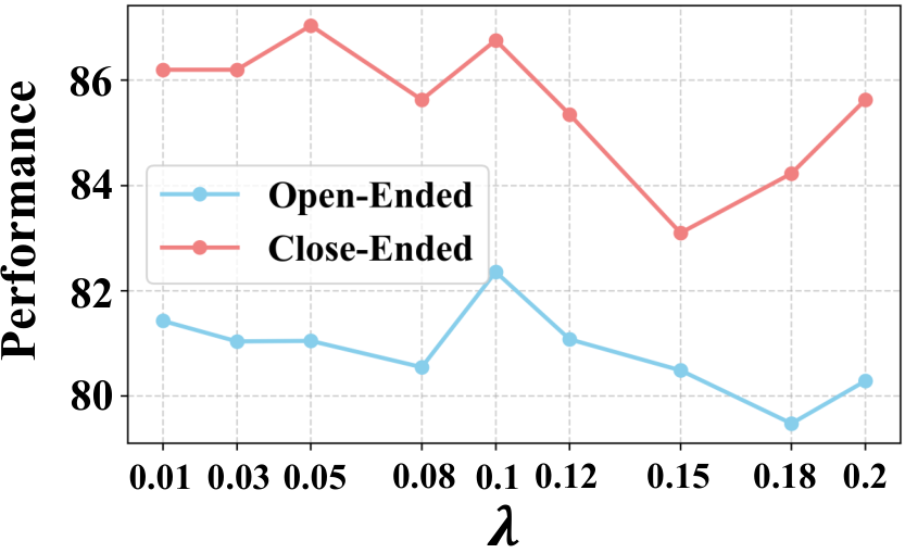
In our final loss in Eq. (12), we use a key hyperparameter to balance the two loss terms. Here, we conduct an analysis to select the optimal value of . Figure 8, illustrate the impact of , which controls the strength of attention alignment tuning. We can observe that on SLAKE, performance peaks at . Beyond this point, the performance declines due to over-alignment and extreme attention distributions. Notably, varies with the scale of datasets and the training epoches, and the values of and fine-tuning epoches for all the datasets are as shown in Table 7.
All the experiments are conducted using four A6000 GPUs.
Appendix D Metrics
D.1 Metrics for Report Generation
We evaluate model performance using commonly used metrics for generation tasks. These include BERTScore Zhang et al. (2019), which measures the similarity between the embeddings of predicted and reference texts, and METEOR Banerjee and Lavie (2005), which evaluates alignment between generated answers and reference texts, accounting for synonyms and stemming. Additionally, we employ ROUGE-L (Lin, 2004), which measures n-gram overlap and the longest common subsequence, and BLEU Papineni et al. (2002), which calculates n-gram precision in the predicted text relative to the reference, focusing on exact matches. In addition, we include the following domain-specific metrics designed for medical report generation:
- •
CheXbert Smit et al. (2020) is an automatic labeler that extracts pathology indicators from radiology reports. We follow Yu et al. (2023) to calculate the CheXbert vector similarity that measures the cosine similarity between pathology indicator vectors derived from ground truth and model-generated reports.
- •
RadGraph Jain et al. (2021) is a tool that extracts entity and relation from radiology reports. We use RadGraph to specifically indicate RadGraph F1, which measures the overlap of clinical entities and their relations extracted from ground truth and model-generated reports.
- •
RaTEScore Zhao et al. (2024) is a recently proposed metric that prioritizes crucial medical entities, including diagnostic outcomes and anatomical details. This metric is robust to complex medical synonyms and sensitive to negation expressions, aligning more closely with human judgment compared to existing metrics.
D.2 Metrics for Attention Distribution
(a) Coverage Score. The Coverage Score measures the proportion of the ground truth region that is covered by the attention map. Let denote the binary mask of the ground truth segment (where for pixels belonging to the ground truth and otherwise) and denote the attention map output by the model. The score is defined as:
where is the thresholded attention map, i.e., if , and otherwise. This metric quantifies how well the attention aligns spatially with the ground truth. In our experiments, we set as .
(b) Intensity Alignment. The Intensity Alignment metric evaluates the average attention intensity within the ground truth region. It is computed as:
This score reflects the degree to which the model focuses its attention on the ground truth segment, considering the intensity values of the attention map.
| Method | Chest X-ray | Abdomen CT | Brain MRI | |||
| Open | Closed | Open | Closed | Open | Closed | |
| LLaVA-Med + LoRA | 76.96 | 89.08 | 79.67 | 81.15 | 79.15 | 79.37 |
| Greedy | 79.53 | 89.92 | 81.50 | 83.61 | 80.57 | 82.54 |
| Beam | 79.83 | 89.92 | 81.76 | 84.43 | 78.90 | 84.12 |
| Nucleus | 80.95 | 87.40 | 79.49 | 79.51 | 79.72 | 80.95 |
| DoLa | 78.53 | 89.92 | 81.50 | 83.61 | 79.89 | 80.95 |
| VCD | 81.39 | 86.55 | 80.54 | 80.33 | 79.62 | 69.84 |
| M3ID | 79.54 | 85.71 | 76.70 | 80.33 | 80.57 | 73.01 |
| AVISC | 80.52 | 87.40 | 81.41 | 78.69 | 80.49 | 85.71 |
| OPERA | 80.19 | 89.92 | 81.15 | 83.61 | 77.55 | 82.54 |
| DAMRO | 79.23 | 88.24 | 80.19 | 83.61 | 75.60 | 80.95 |
| PAI | 79.78 | 89.92 | 80.45 | 81.15 | 81.95 | 80.95 |
| A3Tune (ours) | 82.21 | 89.92 | 83.33 | 84.43 | 82.41 | 87.30 |


| Model | Method | IU-Xray | ||||||
| BLEU | ROUGE-L | METEOR | BERTScore | CheXbert | RadGraph | RaTEScore | ||
| LLaVA-Med-1.5 | LLaVA-Med-1.5 | 1.40 | 12.41 | 16.30 | 84.55 | 38.20 | 7.77 | 41.15 |
| Greedy | 1.04 | 12.15 | 9.87 | 85.43 | 38.04 | 5.43 | 34.97 | |
| Beam | 1.09 | 11.17 | 19.59 | 83.43 | 40.13 | 9.42 | 48.64 | |
| Nucleus | 1.44 | 12.10 | 15.60 | 81.45 | 38.04 | 6.51 | 40.41 | |
| VCD | 1.42 | 12.29 | 15.72 | 84.54 | 36.57 | 6.49 | 39.93 | |
| DoLa | 0.99 | 12.15 | 9.36 | 85.64 | 38.22 | 5.40 | 34.93 | |
| OPERA | 1.13 | 11.49 | 14.63 | 83.76 | 37.38 | 1.41 | 35.96 | |
| AVISC | 1.18 | 11.32 | 16.66 | 83.76 | 35.83 | 6.63 | 40.36 | |
| M3ID | 1.33 | 12.31 | 16.31 | 84.45 | 37.54 | 6.42 | 40.41 | |
| DAMRO | 1.27 | 11.56 | 16.42 | 84.08 | 35.60 | 6.80 | 40.08 | |
| PAI | 1.11 | 12.05 | 10.99 | 85.03 | 37.56 | 5.21 | 34.83 | |
| LLaVA-Med-1.5 + LoRA | LLaVA-Med-1.5 + LoRA | 8.04 | 26.52 | 30.37 | 88.24 | 51.32 | 20.35 | 56.97 |
| Greedy | 9.36 | 27.57 | 27.91 | 88.55 | 52.44 | 21.28 | 58.61 | |
| Beam | 9.54 | 28.41 | 35.40 | 88.45 | 53.70 | 22.43 | 59.65 | |
| Nucleus | 7.80 | 26.72 | 30.33 | 88.28 | 52.73 | 20.85 | 57.84 | |
| VCD | 8.83 | 27.36 | 31.77 | 88.30 | 51.86 | 22.02 | 58.93 | |
| DoLa | 8.93 | 26.94 | 25.74 | 88.42 | 52.27 | 20.63 | 58.10 | |
| OPERA | 9.23 | 27.48 | 34.17 | 88.17 | 51.65 | 21.37 | 57.89 | |
| AVISC | 5.57 | 21.71 | 26.84 | 87.34 | 47.32 | 16.87 | 53.66 | |
| M3ID | 8.44 | 26.21 | 30.86 | 88.20 | 51.13 | 20.77 | 59.37 | |
| DAMRO | 8.21 | 25.77 | 30.58 | 88.09 | 50.10 | 22.33 | 57.31 | |
| PAI | 8.52 | 26.97 | 28.63 | 88.42 | 52.22 | 20.99 | 58.21 | |
| A3Tune (ours) | 10.51 | 28.76 | 35.74 | 88.51 | 53.88 | 23.10 | 59.66 | |
| Model | Method | MIMIC-CXR | ||||||
| BLEU | ROUGE-L | METEOR | BERTScore | CheXbert | RadGraph | RaTEScore | ||
| LLaVA-Med-1.5 | LLaVA-Med-1.5 | 0.98 | 10.73 | 10.95 | 82.29 | 14.11 | 1.83 | 31.90 |
| Greedy | 0.93 | 10.90 | 9.45 | 83.09 | 14.11 | 1.09 | 28.07 | |
| Beam | 1.13 | 10.95 | 13.01 | 82.34 | 12.51 | 1.87 | 32.86 | |
| Nucleus | 0.96 | 10.55 | 10.70 | 78.53 | 14.11 | 1.64 | 31.54 | |
| VCD | 1.00 | 10.93 | 11.31 | 83.11 | 13.46 | 1.97 | 31.75 | |
| DoLa | 0.65 | 9.88 | 7.83 | 83.47 | 14.07 | 1.09 | 28.07 | |
| OPERA | 1.09 | 11.51 | 12.22 | 82.69 | 13.00 | 0.52 | 27.77 | |
| AVISC | 1.16 | 11.14 | 12.30 | 82.61 | 14.11 | 1.97 | 32.20 | |
| M3ID | 1.06 | 11.50 | 11.54 | 83.15 | 13.98 | 2.24 | 32.74 | |
| DAMRO | 1.14 | 11.01 | 12.35 | 82.80 | 13.73 | 2.26 | 32.18 | |
| PAI | 1.12 | 11.67 | 10.63 | 82.80 | 14.05 | 0.98 | 28.07 | |
| LLaVA-Med-1.5 + LoRA | LLaVA-Med-1.5 + LoRA | 3.50 | 16.38 | 18.95 | 85.56 | 21.45 | 9.54 | 40.45 |
| Greedy | 3.50 | 16.49 | 18.71 | 85.54 | 23.43 | 9.63 | 40.49 | |
| Beam | 3.66 | 16.85 | 20.68 | 85.51 | 25.00 | 9.91 | 41.46 | |
| Nucleus | 3.48 | 16.35 | 18.93 | 85.50 | 22.21 | 9.27 | 40.08 | |
| VCD | 3.74 | 16.88 | 19.03 | 85.56 | 22.98 | 9.56 | 40.93 | |
| DoLa | 3.48 | 16.45 | 18.66 | 85.54 | 23.34 | 9.52 | 40.49 | |
| OPERA | 3.56 | 16.77 | 20.10 | 85.46 | 24.31 | 9.81 | 41.33 | |
| AVISC | 3.31 | 16.36 | 18.64 | 85.48 | 23.31 | 9.02 | 40.36 | |
| M3ID | 3.14 | 16.13 | 18.52 | 85.39 | 22.42 | 9.15 | 39.74 | |
| DAMRO | 3.42 | 16.63 | 18.87 | 85.48 | 23.30 | 9.46 | 40.80 | |
| PAI | 3.63 | 16.65 | 18.61 | 85.60 | 24.51 | 9.60 | 40.49 | |
| A3Tune (ours) | 4.22 | 18.02 | 20.69 | 85.75 | 25.37 | 10.52 | 42.15 | |
Appendix E Full Results on Report Generation Benchmarks
We present the comparison results of report generation using LLaVA-Med in Table 8 (IU-Xray) and Table 9 (MIMIC-CXR). These tables include the original results of baselines applied to LLaVA-Med without fine-tuning, where the model performs significantly worse on report generation. For example, in Table 8, the best-performing baseline, M3ID, achieves a BLEU score of 1.40, which is much lower than fine-tuned LLaVA-Med baselines. This highlights the challenge of generating professional medical reports without fine-tuning. As discussed in the experiments section, A3Tune consistently achieves the best performance, outperforming all baselines by a large margin.
Appendix F Fine-grained Effectiveness Analysis
In this experiment, we conduct fine-grained analyses to evaluate the effectiveness of our proposed method across different medical image modalities. Specifically, we examine how our approach improves model performance on Chest X-ray, Abdomen CT, and Brain MRI images from SLAKE. As shown in Table 10, our method outperforms all baselines, particularly on Brain MRI. These results demonstrates the effectiveness of A3Tune across diverse medical images and its generalization ability in medical applications. To explain this improvement, we also include case studies with attention map visualizations for each modality in Section 5.5.
Furthermore, we analyze the VQA types where our method outperforms fine-tuned LLaVA-Med with LoRA across the three image modalities. As shown in Figure 9, our approach improves the model’s performance in three key areas sensitive to image information:
- •
General Radiology Knowledge: Understanding medical modality types and their features.
- •
Anatomical Structures: Recognizing features of key anatomical structures, such as organ count, location.
- •
Abnormalities: Identifying and diagnosing abnormalities based on features like location and color.
These improvements highlight the effectiveness of attention tuning in handling VQA types relying on accurate visual information and interaction.
Appendix G Analysis on LLaVA-Med-1.5
G.1 Attention Biases and Hallucination Issues in LLaVA-Med-1.5
The attention biases we address are not unique to LLaVA-Med but are prevalent across Med-LVLMs. For instance, we include cases from LLaVA-Med-1.5 in this section. Although LLaVA-Med-1.5 is an enhanced version of LLaVA-Med, with improved training data and an increased number of visual tokens (from 256 to 576), the attention biases and hallucination issues persist.
In Figure 10, we visualize the attention biases and corresponding hallucination issues in LLaVA-Med-1.5. As shown, the model often fails to focus on the correct RoIs and generates hallucinated outputs. Even with attention tuning via ControlMLLM, hallucinations persist. For example, in Case (B.3), while the model identifies an abnormality in the liver, it incorrectly classifies it as a liver abscess instead of liver cancer.
These attention biases are common issues in Med-LVLMs, underscoring the need for continued research on emergent Med-LVLMs to mitigate such challenges effectively.
G.2 Experiment Results on LLaVA-Med-1.5
Similar to the LLaVA-Med experiments in Section 5.3, Table 11 and Table 12 show that A3Tune outperforms all baselines across almost all metrics on both IU-Xray and MIMIC-CXR, excelling in both language quality and clinical accuracy. These results underscore A3Tune’ effectiveness in medical applications across diverse Med-LVLMs, demonstrating its strong generalization ability.