Diffusion Self-Weighted Guidance for Offline Reinforcement Learning

Consider an agent that, following an unknown behavior policy $\mu(\mathbf{a}|s)$, interacted with the environment generating samples $(s,\mathbf{a},r,s^{\prime})$ recorded in a dataset $\mathcal{D}_{\mu}$. The goal of offline RL is to estimate the optimal policy $\pi(\mathbf{a}|s)$ from $\mathcal{D}_{\mu}$. Modeling the target policy as a weighted behavior policy in equation 1 is commonplace across various offline RL methods, some of which are presented next.

Constrained policy optimization (Peters et al., 2010; Peng et al., 2019; Nair et al., 2020) regularizes the learned policy to ensure that it remains close to the behavior policy by:

where $Q(s,\mathbf{a})$ is the state-action function that indicates the quality of an action given a state, in terms of the expected future discounted rewards under a specific policy.

Following (Peters et al., 2010; Peng et al., 2019; Nair et al., 2020), it can be shown that the optimal policy $\pi^{*}(\mathbf{a}|s)$ in equation 2 has a weighted structure as in equation 1, given by:

where $Q(s,\mathbf{a})$ represents the Q-values function of the optimal policy. Note that estimating the target policy Q-values requires querying out-of-sample actions.

Implicit Q-learning (IQL) (Kostrikov et al., 2022) avoids querying out-of-sample actions using an in-sample loss based on expectile regression. In this way, it defines an implicit policy that outperforms the behavior policy. Furthermore, IQL employs advantage-weighted regression (Peters and Schaal, 2007; Wang et al., 2018; Peng et al., 2019; Nair et al., 2020) to extract the policy, which can also be interpreted as a weighted behavior policy, given by:

where $A{(s,\mathbf{a})}=Q(s,\mathbf{a})-V(s)$ is the advantage function learned with expectile regression.

Implicit Diffusion Q-learning (IDQL) (Hansen-Estruch et al., 2023) generalizes implicit formulations to the use of an arbitrarily convex function $f$:

thus defining a weighted behavior implicit policy given by

where $w(s,\mathbf{a})=\frac{|f^{\prime}(Q(s,\mathbf{a})-V^{*}(s))|}{|Q(s,\mathbf{a})-V^{*}(s)|}$. Furthermore, IDQL explores different convex functions $f$, such as expectiles (Kostrikov et al., 2022), quantiles (Koenker and Hallock, 2001) and exponential functions.

Diffusion models (DM) approximate an unknown data distribution¹¹ 1 We denote data with the symbol $\mathbf{a}$ (instead of the standard $x$) for consistency, since in our setting the data are the agent’s actions. $q_{0}(\mathbf{a}_{0})$ using a dataset $\mathcal{D}$ by defining a sequence of $k\in\{0,\ldots,K\},K\in\mathbb{N},$ noisy distributions defined as follows:

where $\alpha_{k}$ and $\sigma_{k}$ are predefined noise schedules, s.t., $\mathbf{a}_{K}\sim\mathcal{N}(0,\mathbf{I})$ as $K\to\infty$. Therefore, samples from $q_{0}$ can be obtained by first sampling from $\mathcal{N}(0,\mathbf{I})$, and then solving the reverse diffusion process. In practice, the reverse diffusion is approximated by a model $\epsilon_{\theta}$ that predicts the noise to be removed from a noisy sample $\mathbf{a}_{K}\sim q_{K}$, to produce a target sample $\mathbf{a}_{0}\sim q_{0}$. The training loss for $\epsilon_{\theta}$ is (Ho et al., 2020)

where $\mathbf{a}_{0}\sim q_{0}$, $\epsilon_{0}\sim\mathcal{N}(0,\textbf{I})$, $k\sim\mathcal{U}(1,K)$ and $\mathbf{a}_{k}=\alpha_{k}\mathbf{a}_{0}+\sigma_{k}\epsilon_{0}$. The noise is related to the score function (Song et al., 2021) of the intermediate noisy distribution as follows:

Our motivation for employing diffusion models (DMs) in offline RL stems from two main factors: (1) DMs are highly expressive compared to classical generative models (e.g., Mixture Models), allowing them to model multi-modal action distributions (Chi et al., 2025); and (2) their score-based formulation enables flexible sampling from conditioned or weighted distributions via guidance. In particular, the weighted behavior in equation 1 can be naturally incorporated using DMs, making them well suited for offline RL.

To condition the DM on the states, the noise prediction network can be made an explicit function of the state, that is, $\epsilon(\mathbf{a}_{k},k)=\epsilon(\mathbf{a}_{k},k,s)$. Previous approaches fit a DM $\mu_{\theta}(\mathbf{a}|s)$ to the behavior policy $\mu(\mathbf{a}|s)$, learn the weights $w(s,\mathbf{a})$ as described in Sec. 2.1, and then sample from the target policy via resampling or guidance; these are explained as follows.

Resampling involves first sampling a batch of actions from the learned behavior policy $\mu_{\theta}(\mathbf{a}|s)$, and then resampling them using weights as probabilities of a categorical distribution (Hansen-Estruch et al., 2023; Chen et al., 2023), in a way inspired by importance sampling. Alternatively, one can adopt a greedy policy that simply selects the action that maximizes the weight with the aim of improving performance.

Guidance aims to obtain samples from the target policy by modifying the diffusion, adding a score term approximated by an external guidance network $g_{\phi}$ (Janner et al., 2022; Lu et al., 2023; Mao et al., 2024). The $k$-step score in a diffusion sampling procedure is given by:

where $\{\mathbf{a}_{k}\}_{0}^{K}$ are the noisy versions of the actions, with $\mathbf{a}_{0}$ being the true noise-free action. As shown by (Lu et al., 2023), an unbiased estimate of the guidance score that effectively produces samples from the target distribution should satisfy the following:

where the right-hand term is intractable for most policies and weight functions. Guidance methods that are unbiased towards this objective are referred to as exact guidance methods.

Diffuser (Janner et al., 2022), trains the guidance network with a mean-squared-error objective with respect to Q-values, which produces a biased target policy, in the sense that it does not match the form in equation 5. Conversely, exact guidance methods such as Contrastive Energy Prediction (CEP) (Lu et al., 2023) use a contrastive learning objective that requires querying a batch of out-of-sample actions for each state in the dataset. Lastly, D-DICE (Mao et al., 2024), proposes an in-sample loss to learn the guidance network and uses a guide-then-select approach to obtain samples.

Let us consider a dataset $\mathcal{D}_{A}=\{\mathbf{a}^{(i)}\}_{i=1}^{N}\subset\mathbb{R}^{d}$ of i.i.d. realizations of a random variable $A\sim q(\mathbf{a})$; these will be the agent’s actions. Recall that we aim to sample from the unnormalized target $p(\cdot)$ that relates to $q(\cdot)$ as

where $w:\mathbb{R}^{d}\to\mathbb{R}$ is a known²² 2 Though in offline RL the weight function $w$ has to be learned, we consider $w$ known for now. weight function. Sampling can be achieved by fitting a DM, denoted $\epsilon_{\theta}$, to $q(\mathbf{a})$ trained on $\mathcal{D}_{A}$. Then, in the $k$-th denoising step, the score of the target distribution (referred to as the target score) satisfies:

where $\mathbf{a}_{0}\in\mathcal{D}_{A}$ is a data sample, $\mathbf{a}_{1},\ldots,\mathbf{a}_{K}$ are noisy copies of the data on which the DM is trained, and the subindex $\cdot_{k}$ in the distributions denotes the denoising step. Although $\nabla_{\mathbf{a}_{k}}\log q_{k}(\mathbf{a}_{k})$, referred to as the intermediate score, is provided directly by the DM, estimating the target score in equation 7 is challenging due to the intractability of the right-hand term in the general case (Lu et al., 2023).

Let us consider a random variable (RV) $Z=(A,W)$ given by the concatenation of $A$, describing the actions in the previous section, and $W$, which is given by passing $A$ through the weight function $w(\cdot)$. Since $w(\cdot)$ is a deterministic function of $A$, the distribution of $Z$ is given by the push-forward measure of the distribution of $A$ through the mapping $T:\mathbf{a}\mapsto(\mathbf{a},w(\mathbf{a}))$. With a slight abuse of notation, we denote the push-forward measures corresponding to $p$ and $q$ in equation 6 with the same symbols, i.e. $p(\mathbf{z})=T_{\#}p(\mathbf{a})$ and $q(\mathbf{z})=T_{\#}q(\mathbf{a})$, respectively. Therefore, we have

which, combined with equation 6, give $p(\mathbf{z})\propto q(\mathbf{z})w$. In this new formulation, $w$ is no longer to be considered as a function of a, but rather as a variable for which there are available observations. For clarity of presentation, we define the following function

We can now implement a DM to sample from the augmented variable $Z$. To this end, we first extend the dataset $\mathcal{D}_{A}=\{(\mathbf{a}^{(i)})\}_{i=1}^{N}$ to $\mathcal{D}_{Z}=\{(\mathbf{a}^{(i)},w^{(i)})\}_{i=1}^{N}\subset\mathbb{R}^{d+1}$, where $w^{(i)}=w(\mathbf{a}^{(i)})$ is a weight observation. Notice that the dataset $\mathcal{D}_{Z}$ provides access to the weight function only on the support of the original data in $\mathcal{D}_{A}$. For consistency, we also denote the realizations of $Z$ as $\mathbf{z}^{(i)}=(\mathbf{a}^{(i)},w^{(i)})$.

Therefore, we define a $K$-step diffusion with noise schedule $\{\alpha_{k}\}_{k=1}^{K}$, $\{\sigma_{k}\}_{k=1}^{K}$, and train a noise-prediction DM ${\epsilon}_{\theta}$ for $Z$ using the augmented dataset $\mathcal{D}_{Z}$, minimizing the standard diffusion loss in equation 3. In our notation, this is

where $\mathbf{z}_{0}\sim\mathcal{D}_{Z}$, $\mathbf{z}_{k}=\alpha_{k}\mathbf{z}_{0}+\sigma_{k}\epsilon_{0}$, $\epsilon_{0}\sim\mathcal{N}(0,\textbf{I})$, and $k\sim\mathcal{U}(1,K)$. Algorithm 1 describes our proposed DM training procedure. We emphasize that, in practice, Algorithm 1 is implemented with the expectile weight function.

The proof for Proposition 3.3 follows as an extension of (Lu et al., 2023) to our setting (see Appendix A.1).

The key insight of our proposal is that the intractable term in equation 10 can be recovered directly from the DM described above using the so-called data prediction formula (Efron, 2011; Kingma et al., 2021) given by:

Using equation 11, and since the extraction function $\phi_{w}(\cdot)$ is linear, the target score $\nabla_{\mathbf{z}_{k}}\log p_{k}(\mathbf{z}_{k})$ in equation 10 can be computed with the proposed DM, as stated in Theorem 3.5 (proof in Appendix A.2).

Our method is referred to as Self-Weighted Guidance (SWG), since the DM samples from the target distribution $\mathbf{z}_{0}\sim p(\mathbf{z}_{0})$ by guiding itself, that is, the guidance signal is a function of the same model (see Algorithm 2). SWG provides an elegant way of performing exact guidance, since it computes gradients directly on the DM $\epsilon_{\theta}$ instead of an external guidance network with a dedicated —and possibly intricate— loss function (see Sec. 4). This translates to not having to train a separate guidance network, thereby simplifying the training pipeline. Sec. 4 provides a theoretical comparison between SWG and other DM-based guidance approaches to offline RL, the results of which are summarized in Table 1.

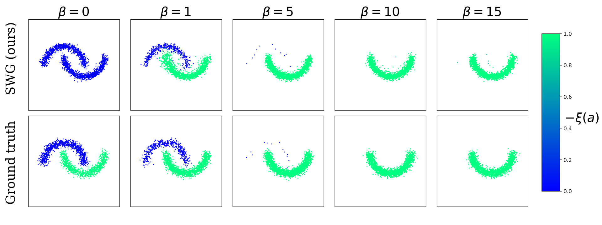
We considered the toy experiments from (Lu et al., 2023), which use a weight function $w(\mathbf{a})=\exp(-\beta\xi(\mathbf{a}))$, where $\xi(\mathbf{a})$ is an energy function, and $\beta$ is the inverse temperature coefficient. Figures 2 and 3 show SWG samples from a spiral and an 8-Gaussian-mixture distributions, respectively, and offer a qualitative assessment of its performance. In both cases, samples closely matching the ground truth for different values of $\beta$ suggest that SWG was able to sample from the target distributions, thus learning the relationship between the data distribution and the weights in both cases. The reader is referred to the Appendix B.1 for further details and more examples with different target distributions.

Using the D4RL benchmark (Fu et al., 2021), we implemented two variants of the proposed method: SWG as described above, and SWG-R, which includes action resampling on top of our method. We considered the following methods as benchmarks:

• •

  Classical offline RL: CQL (Kumar et al., 2020) and IQL (Kostrikov et al., 2022)

• •

  Diffusion-based resampling: SfBC (Chen et al., 2023) and IDQL (Hansen-Estruch et al., 2023)

• •

  Diffusion-guided: Diffuser (Janner et al., 2022), D-DICE (Mao et al., 2024), and QGPO (CEP) (Lu et al., 2023)

• •

  D-QL (Wang et al., 2022), which trains a DM using Q-values as regularization term

Furthermore, our experiments are performed across four task groups:

1. 1.

   Locomotion: the main offline RL benchmark, which features moving an agent across a plane.

2. 2.

   Ant Maze: a more challenging task, where an ant agent is guided through a maze to reach a target.

3. 3.

   Franka Kitchen: involves goal-conditioned manipulation in a realistic kitchen environment.

4. 4.

   Adroit Pen: focuses on high-dimensional dexterous manipulation to reorient a pen.

These experiments were conducted with the expectile weight proposed in IDQL (Hansen-Estruch et al., 2023) modified as detailed in Sec. 5, and using $K=15$ diffusion steps. See Appendix B.2 for more details.

The results shown in Table 2 reveal that the resampled version of our proposal SWG-R provided competitive performance over state-of-the-art DMs in the challenging environment tasks from Franka Kitchen and Adroit Pen. In Ant Maze, SWG-R also reported very competitive figures, outperforming all methods except D-DICE. However, in locomotion tasks, both SWG and SWG-R achieved average performance compared to previous methods. Also, note that SWG outperformed classical offline RL methods such as CQL and IQL in most tasks.

Based on the D4RL results, we argue that SWG-R offers a tradeoff between having a simpler training setup with fewer components than current DM guidance-based approaches at the cost of a lower performance with respect to the top-performing method, D-DICE (Mao et al., 2024), for the particular case of the Locomotion dataset. Moreover, incorporating resampling was pivotal for the enhanced performance of SWG-R over SWG. This addition strengthened the effectiveness of our framework, similarly to previous approaches. However, it is worth noting that the performance gain of SWG-R comes at the cost of an expanded hyperparameter search space during inference (see Appendix B.2). Additionally, we remark that the resampling was performed using the separate weight model $w$ (i.e., expectile weights).

We then evaluated SWG’s performance under different weight formulations in Sec. 5. This test was conducted on D4RL locomotion, using the same model architecture and hyperparameter tuning to ensure a fair comparison. Furthermore, we also tuned the guidance scale in each case to find the best possible performance. The weight formulations were implemented as follows:

• •

  Expectile weight: Learnt with the same setup adopted in the main results, described in Sec. 5.

• •

  Exponential expectile weight: We used the same setup as for IDQL expectile weights, and considered a temperature $\beta=3$ to exponentiate the advantage function $e^{\beta{A(s,\mathbf{a})}}$. To ensure stability during training, we clipped the exponential weights to $(0,80]$.

• •

  Linex weight: We followed IDQL (Hansen-Estruch et al., 2023), and used $\alpha=1$.

The results, shown in Table 3, reveal that expectile yielded the best performance, with the exponential expectile showing moderate performance, and lastly Linex performing substantially worse. We conjecture that this is due to the training instability introduced by the exponential weights, in general. Most importantly, these results are consistent with the findings reported in IDQL (Hansen-Estruch et al., 2023).

We also studied the effect of using a fixed guidance scale across all tasks, without tuning $\rho$ for each task individually. Recall that the choice of the guidance scale $\rho$ controls the strength of the guidance score, which translates into a sharper target distribution concentrated around high-value weights. This effect can be seen in the modified noise prediction $\hat{\epsilon}:={\epsilon}_{\theta}(\mathbf{z}_{k},k)-\rho\sigma_{k}\nabla_{\mathbf{z}_{k}}\log{(\phi_{w}(\frac{\mathbf{z}_{k}-\sigma_{k}{\epsilon}_{\theta}(\mathbf{z}_{k},k)}{\alpha_{k}}))}={\epsilon}_{\theta}(\mathbf{z}_{k},k)-\sigma_{k}\nabla_{\mathbf{z}_{k}}\log{(\phi_{w}((\frac{\mathbf{z}_{k}-\sigma_{k}{\epsilon}_{\theta}(\mathbf{z}_{k},k)}{\alpha_{k}})^{\rho}))}$. We conduct these experiments using expectile weights, which, as shown in Sec. 6.3, yield superior performance.

Overall, from Tables 4 and 5, we observe that the best performance was generally achieved with $\rho=10$ or $\rho=15$. As expected, using low guidance scales ($\rho<5$) resulted in suboptimal performance, as the guidance signal was not sufficiently strong. On the other hand, employing large guidance scales ($\rho>20$) led to poorer performance, since an overly strong guidance signal tends to produce out-of-distribution samples.

Since SWG requires computing gradients through DM, we investigated its scalability properties through two experiments examining both depth and width scaling of its networks. For depth scaling, we used a simple multilayer perceptron (MLP) with a hidden dimension of 2056 and measured the inference time across varying numbers of layers. For width scaling, we used a fixed 4-layer MLP with varying hidden dimension, measuring the average inference time accordingly (see the Appendix B.3).

As shown in Figures 5 and 5, SWG exhibited a linear scaling with respect to model depth and exponential scaling with respect to the width scaling (hidden dimension). Additionally, and as expected, sampling with guidance (i.e., computing gradients) translates into larger inference times. However, qualitatively, we can observe that both sampling methods scale at a similar rate. Note that scaling issues related to gradient computation can be easily avoided by designing the DM to output the weight component in its early layers. This allows gradients to be computed with respect to a fixed module, without requiring backpropagation through the entire model. Consequently, the additional computational overhead of SWG remains constant, even as the sub-component of the model responsible for action generation increases in scale.

The training time remains essentially the same as that of the related methods (Hansen-Estruch et al., 2023; Mao et al., 2024) when using a similar architecture. The SWG training time measurements are reported in the Appendix B.4.

References

- Layer normalization. arXiv preprint arXiv:1607.06450. Cited by: §B.2.
- JAX: composable transformations of Python+NumPy programs External Links: Link Cited by: §B.4.
- Offline reinforcement learning via high-fidelity generative behavior modeling. In International Conference on Learning Representations, Cited by: §1, §2.2, 2nd item.
- Diffusion policy: visuomotor policy learning via action diffusion. The International Journal of Robotics Research 44 (10-11), pp. 1684–1704. Cited by: §1, §2.2.
- Diffusion models beat GANs on image synthesis. Advances in Neural Information Processing Systems 34, pp. 8780–8794. Cited by: §5, §7.
- Tweedie’s formula and selection bias. Journal of the American Statistical Association 106 (496), pp. 1602–1614. Cited by: §A.2, §3.3.
- D4RL: datasets for deep data-driven reinforcement learning. arXiv preprint arXiv:2004.07219. External Links: Link Cited by: §B.2, §B.2, §6.2, Table 2.
- Off-policy deep reinforcement learning without exploration. In Proceedings of the International Conference on Machine Learning, Vol. 97, pp. 2052–2062. Cited by: §1.
- Addressing function approximation error in actor-critic methods. In Proceedings of the International Conference on Machine Learning, Vol. 80, pp. 1587–1596. Cited by: §B.2.
- IDQL: implicit Q-learning as an actor-critic method with diffusion policies. arXiv preprint arXiv:2304.10573. External Links: Link Cited by: §B.2, §B.2, §B.2, §1, §1, §1, §2.1, §2.2, §5, §5, 2nd item, 3rd item, §6.2, §6.3, §6.5.
- Flax: a neural network library and ecosystem for JAX External Links: Link Cited by: §B.4.
- Denoising diffusion probabilistic models. Advances in Neural Information Processing Systems 33, pp. 6840–6851. Cited by: §1, §2.2.
- Planning with diffusion for flexible behavior synthesis. In Proceedings of the International Conference on Machine Learning, Vol. 162, pp. 9902–9915. Cited by: §B.2, §1, §2.2, §2.2, Table 1, 3rd item.
- Adam: a method for stochastic optimization. In International Conference on Learning Representations, Cited by: §B.1, §B.2, §B.2.
- Variational diffusion models. In Advances in Neural Information Processing Systems, Vol. 34, pp. 21696–21707. Cited by: §A.2, §3.3, §4.
- Quantile regression. Journal of Economic Perspectives 15 (4), pp. 143–156. External Links: Document Cited by: §2.1.
- Offline reinforcement learning with implicit Q-learning. In International Conference on Learning Representations, Cited by: §B.2, §1, §1, §2.1, §2.1, §4, §5, §5, 1st item.
- JAXRL: Implementations of Reinforcement Learning algorithms in JAX. External Links: Document, Link Cited by: §B.4.
- Stabilizing off-policy Q-learning via bootstrapping error reduction. In Advances in Neural Information Processing Systems, Vol. 32. Cited by: §1.
- Conservative Q-learning for offline reinforcement learning. In Advances in Neural Information Processing Systems, Vol. 33, pp. 1179–1191. Cited by: 1st item.
- Offline reinforcement learning: tutorial, review, and perspectives on open problems. arXiv preprint arXiv:2005.01643. External Links: Link Cited by: §1.
- Efficient planning with latent diffusion. In International Conference on Learning Representations, Cited by: §B.2.
- Diffusion-LM improves controllable text generation. In Advances in Neural Information Processing Systems, A. H. Oh, A. Agarwal, D. Belgrave, and K. Cho (Eds.), Cited by: §7.
- Continuous control with deep reinforcement learning. In International Conference on Learning Representations, Cited by: §B.2.
- Contrastive energy prediction for exact energy-guided diffusion sampling in offline reinforcement learning. In International Conference on Machine Learning, pp. 22825–22855. Cited by: §A.1, §B.1, §B.2, §1, §2.2, §2.2, §2.2, §3.1, §3.3, Table 1, §4, §4, 3rd item, §6.1.
- Diffusion-DICE: in-sample diffusion guidance for offline reinforcement learning. In The Thirty-eighth Annual Conference on Neural Information Processing Systems, Cited by: §B.2, §1, §1, §2.2, §2.2, Table 1, §4, §4, 3rd item, §6.2, §6.5.
- AWAC: accelerating online reinforcement learning with offline datasets. arXiv preprint arXiv:2006.09359. Cited by: §1, §1, §2.1, §2.1, §2.1.
- Improved denoising diffusion probabilistic models. In International Conference on Machine Learning, pp. 8162–8171. Cited by: §B.1.
- Flow q-learning. In Forty-second International Conference on Machine Learning, Cited by: §B.2.
- PyTorch: an imperative style, high-performance deep learning library. In Advances in Neural Information Processing Systems, Vol. 32. Cited by: §B.4.
- Advantage-weighted regression: simple and scalable off-policy reinforcement learning. arXiv preprint arXiv:1910.00177. External Links: Link Cited by: §1, §2.1, §2.1, §2.1.
- Relative entropy policy search. In Proceedings of the AAAI Conference on Artificial Intelligence, pp. 1607–1612. Cited by: §2.1, §2.1.
- Reinforcement learning by reward-weighted regression for operational space control. In Proceedings of the International Conference on Machine Learning, Vol. 227, pp. 745–750. Cited by: §1, §2.1.
- U-net: convolutional networks for biomedical image segmentation. In Medical Image Computing and Computer-Assisted Intervention, pp. 234–241. Cited by: §B.2.
- Deep unsupervised learning using nonequilibrium thermodynamics. In International Conference on Machine Learning, pp. 2256–2265. Cited by: §1.
- Score-based generative modeling through stochastic differential equations. In International Conference on Learning Representations, Cited by: §B.2, §1, §2.2.
- Dropout: a simple way to prevent neural networks from overfitting. Journal of Machine Learning Research 15 (56), pp. 1929–1958. Cited by: §B.2.
- Exponentially weighted imitation learning for batched historical data. In Advances in Neural Information Processing Systems, Vol. 31. Cited by: §2.1.
- Diffusion policies as an expressive policy class for offline reinforcement learning. In International Conference on Learning Representations, Cited by: §1, 4th item.
- Critic regularized regression. In Advances in Neural Information Processing Systems, Vol. 33, pp. 7768–7778. Cited by: §1.
- Offline RL with no OOD actions: in-sample learning via implicit value regularization. In International Conference on Learning Representations, Cited by: §1.
Appendix A Proofs and derivations
A.1 Proof of Proposition 3.3: computation of the target score
We follow the derivation utilized in (Lu et al., 2023).
Let us express the normalizing constant of as
Recall that extracts the component of . Then, we have:
According to the definition of diffusion models, we have:
and finally
A.2 Proof of Theorem 3.5
Recall that we want to sample from in equation 10.
Let us assume that the weight function is known, so we have access to a labeled dataset consisting of samples . We suppose a step diffusion process over , as , .
To address the problem in Equation equation 4, let us assume that we train a noise-predicting diffusion model on the data , , , parametrized by . Then, the optimal diffusion model is defined by the following optimization problem.