Deep Koopman operator framework for causal discovery
in nonlinear dynamical systems
Abstract
We use a deep Koopman operator-theoretic formalism to develop a novel causal discovery algorithm, Kausal. Causal discovery aims to identify cause-effect mechanisms for better scientific understanding, explainable decision-making, and more accurate modeling. Standard statistical frameworks, such as Granger causality, lack the ability to quantify causal relationships in nonlinear dynamics due to the presence of complex feedback mechanisms, timescale mixing, and nonstationarity. This presents a challenge in studying many real-world systems, such as the Earth’s climate. Meanwhile, Koopman operator methods have emerged as a promising tool for approximating nonlinear dynamics in a linear space of observables. In Kausal, we propose to leverage this powerful idea for causal analysis where optimal observables are inferred using deep learning. Causal estimates are then evaluated in a reproducing kernel Hilbert space, and defined as the distance between the marginal dynamics of the effect and the joint dynamics of the cause-effect observables. Our numerical experiments demonstrate Kausal’s superior ability in discovering and characterizing causal signals compared to existing approaches of prescribed observables. Lastly, we extend our analysis to observations of El Niño-Southern Oscillation highlighting our algorithm’s applicability to real-world phenomena. Our code is available at https://github.com/juannat7/kausal.
Keywords:
Machine Learning, ICML1 Introduction
Causal discovery seeks to disentangle the underlying cause-effect mechanisms of physical processes, which is crucial for improved scientific understanding (Aloisi et al., 2022; Cattry et al., 2025; Roesch et al., 2025; Williams et al., 2025). Since performing interventions to detect causality is often infeasible in many domains, there is a great interest to develop data-driven causal discovery methods (Granger, 1969; Hyvärinen et al., 2010; Runge, 2020, e.g.,). However, they tend to operate under certain assumptions, such as time-invariance, stationarity, and linearity (Granger, 1969; Runge et al., 2019; Bareinboim et al., 2022; Camps-Valls et al., 2023), which limit their applicability.11 1 Causal discovery is different from causal effect estimation, where the latter aims to quantify the causal effect between variables for an existing (either discovered or assumed) causal graph. For instance, these simplifications fail while examining nonlinear systems due to the presence of complex feedback mechanisms, spatial autocorrelation, and timescale mixing (Lorenz, 1963; Rupe & Crutchfield, 2024).
In general, there are two categories of approaches for inferring causal relationships in nonlinear dynamical systems: i) using information flow to identify causal influence among variables and subspaces (Granger, 1969; Liang & Kleeman, 2005; Majda & Harlim, 2007; James et al., 2016; Tank et al., 2021); and ii) performing a lifting transformation to project the system of interest to a higher-dimensional space where causal effects can be investigated more easily (Lorenz, 1991; Sugihara et al., 2012; Gilpin, 2024; Butler et al., 2024). Thus, we pose our research question: Can we combine these two principles to apply linear causal analysis methods in nonlinear systems?
A natural foundation for us to start answering this question is Koopman theory (Koopman, 1931; Mezić, 2013; Brunton et al., 2022), which states that finite nonlinear dynamics can be represented with an infinite-dimensional linear operator acting on the space of all possible measurement functions. This formalism presents a significant opportunity for the application of standard linear methods for system analysis, estimation, and control (Brunton et al., 2025). Recent work by Rupe et al. (2024) has established a theoretical foundation linking Koopman theory to causal analysis for dynamical systems using prescribed embeddings. Simultaneously, efficiently and effectively estimating optimal embeddings has been enabled by rapid advances of deep learning in high-dimensional settings (Brunton et al., 2016; Lusch et al., 2018; Wang et al., 2022). Therefore, data-driven Koopman operator methods have seen a surge in interest, especially for spatiotemporal analysis in a number of fields (Kutz et al., 2018; Azencot et al., 2020; Rice et al., 2021; Froyland et al., 2021; Lintner et al., 2023; Lamb et al., 2024; Nathaniel & Gentine, 2025).
Main contributions. In this paper, we leverage ideas from deep learning, Koopman theory, and causal inference. Our main contributions can be summarized as follows:
- •
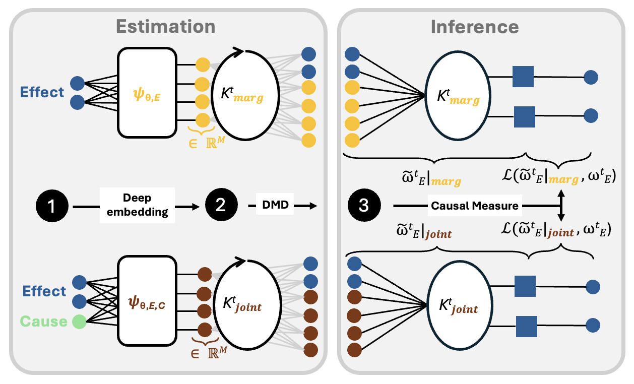
We introduce a novel deep Koopman operator-based causal discovery framework, Kausal, as illustrated in Figure 1.
- •
We show that Kausal infers a better representation of the basis functions through deep learning, as opposed to existing prescribed approaches, which leads to a more accurate and meaningful causal analysis in high-dimensional nonlinear systems.
- •
We successfully apply Kausal to both idealized models and real-world phenomena highlighting the algorithm’s scalability and generalizability.
2 Methodology
2.1 Background
In this section, we follow Rupe et al. (2024) to briefly introduce the mathematical background and the necessary notation to introduce our novel causal algorithm in Section 3.
Dynamical systems. Dynamical systems theory describes the evolution of a system over time, with the system state represented as a point in a phase space, , which we assume to be in the Euclidean space . Throughout this paper variables are treated as vectors unless explicitly stated otherwise.
Flow maps. Time-evolution of states is defined through a set of functions called flow maps that carries the phase space back onto itself. For an initial state , flow maps evolve through time t, given by . The orbit of a state is the set , representing the trajectory of the system over the time domain . Although we denote the initial state as , writing with the initial state would be equivalent. For simplicity, we also restrict our analysis to autonomous dynamical systems characterized by time-independent flow maps.
Ordinary differential equations. In a deterministic setting, the evolution of over time can be described through ordinary differential equations (ODEs) of the form:
| (1) |
where is an arbitrary function and the solution depends on the initial condition at time .
Components. To formalize the idea of causality in a dynamical system, we need to define different components of the system which can impact each other. For an -dimensional phase space (i.e. degrees of freedom) as described above, we partition the space into disjoint system component subspaces as with and , where .
Reproducing Kernel Hilbert Spaces (RKHS). Koopman operators (described in the next section) act on functions rather than directly on system states, mapping one function to another by evolving it under the system dynamics. To ensure the operations of the Koopman operator are mathematically consistent and computationally feasible, we therefore require a well-defined function space. For data-driven analysis, a natural choice of function spaces is reproducing kernel Hilbert spaces.
A RKHS is a Hilbert space of functions such that the evaluation is continuous for each point . This requires the existence of a kernel function such that and . The Moore-Aronszajn theorem (Aronszajn, 1950) implies that a positive definite kernel function defines a unique RKHS, so we use the notation unambiguously. We will express the kernel in terms of an associated feature map , namely . The kernel is constructed as the tensor product of the kernels , which are the kernel functions for each component of the partitioned phase space . For a subspace given we define the component observable function subspace which is itself a RKHS. Thus, is given through the kernel:
| (2) | ||||
for all . We summarize key features of RKHS relevant to the Koopman framework in Table S1.
2.2 Koopman theory
Koopman operator. Koopman theory provides a global linearization of high-dimensional nonlinear dynamical systems (Koopman, 1931; Brunton et al., 2022). Specifically, the nonlinear temporal evolution of system states is represented as a linear flow in the evolution of system observables. The map from system states to observables is given by a function, .
The Koopman operator therefore acts as a time shift t on an observable :
| (3) |
We need Koopman operators acting on to be bounded to ensure the continuity of the time-evolution of , i.e. . This property is given by defining the Koopman operator over a RKHS (Kostic et al., 2022; Rupe et al., 2024).
Observables. Obtaining observables in which the nonlinear dynamics appear approximately linear is an open challenge (Brunton et al., 2022). Existing works often rely on a set of -dimensional dictionary functions spanning a finite-dimensional Hilbert space , such as Gaussian, and Random Fourier features (Rahimi & Recht, 2007, RFF;), Polynomial, Time Delay (Abarbanel et al., 1994, TDF;). Note that these dictionary functions are the previously defined feature maps. Often these functions may not be sufficiently expressive to represent complex dynamics (Kostic et al., 2022). Nonetheless, deep learning provides a natural framework for inferring the optimal high-dimensional embedding, which constitutes one of the goals of this paper.
In this paper, we compute a finite-rank approximation of the Koopman operator with dictionary functions that are learned using different neural network-based encoder-decoder architectures. Since we use appropriate regularizations and activations, namely the bounded sigmoid function, we ensure that the observables are finite. As a result, the kernel function is also bounded, i.e., for all (Aronszajn, 1950; Caponnetto & De Vito, 2007; Kostic et al., 2022). The size of our encoder final layer’s output vector determines the dimensionality of , which is the number of learned dictionary functions.
Dynamic mode decomposition. To estimate the Koopman operator we use dynamic mode decomposition (DMD), which solves a least-squares regression problem to identify a finite-dimensional linear representation of the system dynamics. Using dictionary functions defined as,
| (4) |
we construct data matrices consisting of observables for pairs of data points , denoted as and (t time shifted):
| (5) |
| (6) |
Assuming there exists a unique linear operator that satisfies , where , we can define the least-squares regression problem as:
| (7) | ||||
The full rank least-squares solution is given as:
| (8) |
where is the pseudo-inverse of . A low-rank approximation is also feasible with matrix projection onto dominant modes using e.g., SVD. Note that is an approximation and converges to the Koopman operator for (Korda & Mezić, 2018).
3 Causal discovery
Here we connect principles of causal discovery to the deep Koopman framework introduced in the last section.
3.1 Causal discovery in dynamical systems
Structural dynamical causal models. In statistical terms, causal mechanisms are described through structural causal models (SCM), where a system of random variables are expressed as an arbitrary function of their direct parents (causes) and an exogenous distribution of noise (Peters et al., 2022):
| (9) |
For dynamical systems, we can extend SCM for a collection of ODEs (Equation 1) to define structural dynamical causal models (SDCM) (Rubenstein et al., 2018; Peters et al., 2022; Boeken & Mooij, 2024):
| (10) |
where .
Causal graph. The structural assignment of the SDCM induces a directed acyclic graph (DAG) over the variables . includes nodes for every and directed edges if . The corresponding DAG is visualized in Figure 2.

Causal mechanism. Using the previously defined framework of component subspaces for dynamical systems, we partition the phase space of a system into components:
| (11) |
representing the effect, cause, and remainder components, respectively. Each state is projected into the effect component using coordinate projections , and the evolution of is tracked through the component flow map:
| (12) |
This framework is flexible enough to allow for multipartite causal analysis, i.e., multiple causal factors and , by combining them into a single component .
Causal influence. The existence of a dynamical causal relationship at time t is determined by whether the state of the effect component depends on the initial state of the cause component, i.e., dynamically causally influences at time t. Mathematically we write this as:
| (13a) | ||||
| (13b) | ||||
where Equation 13b implies does not dynamically causally influence .
3.2 Causal discovery with deep Koopman operators
Estimating dynamical causality directly is challenging for nonlinear dynamical systems, requiring carefully crafted counterfactual analysis (Merlis, 2014).
Koopman causal influence. Fortunately, we can rephrase dynamical causality using the Koopman framework, where it is represented by the linear evolution of observables in function spaces. This formulation necessitates that the observables associated with individual components form closed subspaces in the full RKHS that represents the joint dynamical system. We argue that causal relationships in the state space also induce distinguishable patterns in the flow of functions .
For instance, if , then the application of the Koopman operator on the effect observables will inherit this dependence which is expressed as . We define this as Koopman causally influences which is denoted by . Correspondingly, if does not Koopman causally influence at time , it is denoted by where . In summary, dynamical causality and Koopman causality at time turn out to be equivalent. Namely, if and only if . The proof of this can be found in Theorem III.2 in Rupe et al. (2024).
Marginal and joint models. The data-driven measure of Koopman causality leverages the DMD algorithm. Our method involves fitting two distinct DMD models to evolve functions in : i) a marginal model restricted to functions from the subspace ; and ii) a joint model which utilizes functions from the joint subspace incorporating both the effect and cause components. Our algorithm therefore requires a dataset consisting of triplets , where and are the time-shift of and the data time index respectively. We split this dataset into sets of training and test triplets.
We can now define the marginal and joint models, where the addition of identity observables on (Brunton et al., 2016), , empirically improves the performance of our algorithm:
| (14) |
where the matrices and are formed from applying the marginal and joint dictionaries to the training data or , respectively.
Given this setup, our Koopman operators and are not square matrices. We approximate the time-shifted test function through the marginal and joint models given by:
| (15) |
and
| (16) |
where .
Causal measure. The causal measure is defined as,
| (17) | ||||
where the difference in errors between the marginal and joint models is calculated over all data points :
| (18) |
Hence, if the joint model has a significantly lower error, it suggests that contains causal information about . This also implies that if , there is minimal causal influence from on at time t.
Conditional forecasting. Computationally, estimating at each time shift t is expensive. Thus, we perform conditional forecasting, which preserves the structure of marginal and joint models for reasonable t. Feeding the predicted outputs back as identity observables enables efficient exploration of causal dynamics over time. However, it is not true forecasting because we supply data from the test dataset to construct the non-identity observables. Specifically, starting with an initial value of from the test data we can define the first and following conditional predictions for the marginal model as:
| (19) |
Given an additional initial value for we follow the same procedure with necessary adjustments to the dictionary functions to obtain conditional forecasts for the joint model.
4 Experiments
We use this section to empirically demonstrate Kausal’s performance and its application to identify and characterize causal mechanisms in high-dimensional nonlinear systems. Our algorithm runs with a PyTorch backend, and the code is available at https://github.com/juannat7/kausal. Code snippets can be found in Appendix B and additional details on the experimental setup and results in Appendix C, D.
4.1 Coupled Rössler oscillators
We begin our exposition with the coupled Rössler oscillators, a 6-dimensional system described as:
| (20a) | ||||
| (20b) | ||||
where are prescribed parameters and the coupling terms. Setting naturally partitions the variables into . Here, we use multilayer perceptrons (MLP) as our deep estimators for the observables, represented as a -dimensional feature vector of the encoder final layer’s output (see Appendix C.1).
Causal measure estimation. First, we estimate causal measures as defined in Equation 18 where the measure for each unique time shift is estimated across data points. As illustrated in Figure 3, Kausal is able to evaluate statistically significant22 2 See Algorithm 1 with . causal signals in the true direction () when compared with the non-causal case (). For completeness, we also plot the causal measure using an RFF kernel () following Rupe et al. (2024).

Performing conditional forecasting. We also illustrate the concept of conditional forecasting formalized earlier in Equation 19, starting with . As shown in Figure 4, the inclusion of (i.e., the joint model) is crucial in capturing dynamics in the true causal direction, whereas its exclusion (i.e., the marginal model) leads to significant deviations. Conversely, in the non-causal direction, both the marginal and joint models make no perceptible difference in forecasting as .


Optimal kernel selection. Robust estimation of observables is crucial for the accurate representation of nonlinear dynamics in . In order to study this notion, we perform joint forecasts using either a prescribed or a learnable dictionary of functions, , for varying dimensionality . As illustrated in Figure 5, joint forecasts utilizing reproduce the true dynamics more accurately (expected behavior), even beyond the training set and for low . In contrast, joint forecasts using , even with high , struggle to capture the underlying dynamics, underscoring the limitations of prescribing dictionary functions rather than directly learning them from data.


4.2 Reaction-diffusion equation
We now showcase Kausal’s scalability to high-dimensional settings and underscore the notion of uncertainty quantification of causal measures using a 2D nonlinearly coupled reaction-diffusion process described as:
| (21) | ||||
where are prescribed parameters, the 2D Laplace operator (), and the coupling terms. The states () include components of the horizontal velocity. Here, we set , such that the variables are naturally partitioned into . In our setup, we use convolutional neural networks (CNN) as our deep estimators for the observables, represented as a -dimensional feature map of the encoder final layer’s output (see Appendix C.2 for additional details).
Uncertainty quantification of causal measures. Our finite approximation of linear flow in is imperfect, and therefore, capturing its representation uncertainty is crucial. To this end, we fit a number of CNN kernels to form an ensemble, where we maintain the dimensionality () but randomly initialize the learnable weights. In Figure 6, Kausal is able to extract statistically significant causal signals in the true direction () when compared with the non-causal case () as . The ensemble spread is represented as the shaded region around the mean solid line. Note that due to small state values, we scale the causal measure to and negative values of the causal measure are due to an insignificant causal signal.

4.3 ENSO model
As a final experiment, we illustrate Kausal’s generalization to real-world phenomena using an example from climate science, El Niño–Southern Oscillation (ENSO). ENSO is an important source of predictability in the climate system (Wang & Picaut, 2013). As such, a robust understanding of its mechanism and how it evolves in a changing climate is of widespread importance. Due to its major societal impacts, this is especially true for explainable decision making in critical sectors such as agriculture and disaster preparedness (Glantz et al., 1987; Callahan & Mankin, 2023, e.g.,).
We first apply Kausal to analyze a well-known ENSO physics-based dynamical model (Jin, 1997) defined as:
| (22) | ||||
where are prescribed parameters, is a damping coefficient regulating the strength of nonlinearity, and are the coupling terms. The states include anomalies in sea surface temperature and thermocline height in the eastern and western equatorial Pacific, respectively. For notational uniformity, we partition and . However, this does not imply as long as the coupling terms are non-zero, which is the case throughout our exposition. In our setup, we use MLP as our deep estimator for the observables, represented as a -dimensional vector of the encoder final layer’s output.


Linear stability analysis. Setting in Equation 22 linearizes the dynamics such that several evaluations could be performed, including stability analysis. This is crucial for identifying bifurcation, or tipping points of the system. The full linear stability analysis, including the bifurcation diagram, are described and illustrated in Figure S4. Given a prescribed set of parameters, the critical point corresponds to a stable periodic attractor. Meanwhile, and represent dissipative and diverging oscillations, respectively. Here, we only consider physically realistic oscillatory dynamics defined in -regimes where .
In Figure 7, Kausal reveals accurate linear analysis across -regimes that induces dissipative, stable, or diverging oscillatory ENSO dynamics. For instance, in the critical delta region where , our causal measures show identical peaks with consistent periodicity. Whereas in the dissipative (or diverging) dynamics, our causal measures reveal decreasing (or increasing) influence in the direction. This is physically consistent with the model as both and are exerting coupled feedback, and partly governed by .
Capturing nonlinearity strength. We perform similar analysis in the stable region of , but vary nonlinearity by setting . As illustrated in Figure 8, we note two physically consistent observations in the causal measure: (a) oscillatory dynamics (insofar ), and (b) a dampening pattern as nonlinearity strengthens, as evidenced by the slower rate of change in and smaller magnitude of peaks. Overall, a robust identification of weakly or strongly coupled variables within a system, as demonstrated by Kausal, is crucial for better understanding, effective control, and accurate forecasting of dynamics.


4.4 Kausal in the wild
Lastly, we demonstrate the feasibility of Kausal to study ENSO dynamics using ocean reanalysis products from the European Centre for Medium-Range Weather Forecasts (Zuo et al., 2019, ECMWF;). Real-world dataset are often sparse and noisy (Nathaniel et al., 2023; Kim et al., 2024), and leveraging physics-informed priors through causal discovery has been shown to be useful for various tasks including for emulation (Iglesias-Suarez et al., 2024). Preliminary results as illustrated in Figure 9 are promising. We find that Kausal is able to track the emergence of ENSO events as represented by . Specifically, warm-phase El Niño events (red shading in Figure 9) result from an increase in , weakening the Walker circulation and leading to a decrease in . Cold-phase La Niña events follow a similar pattern but in the opposite direction (blue shading in Figure 9). See Appendix C.3 for more details. The estimated causal measure captures major El Niño events in 1982–83, 1997–98, and 2014–16, representing some of the strongest in recorded history (Glantz et al., 1987; McPhaden, 1999; Hu & Fedorov, 2017). Additionally, Figure 9 highlights Kausal’s improved performance with respect to existing work that uses prescribed dictionary functions (Wang et al., 2022; Rupe et al., 2024, e.g.,).
This analysis represents a first step in contributing to ongoing research on possible state changes of ENSO due to increasing ocean temperatures which could have major global impacts (Aiken et al., 2013; Bayr et al., 2024, e.g.,).
4.5 Baselines
In the following, we compare Kausal to a range of baseline causal discovery methods across two tasks: (i) causal direction identification, and (ii) causal magnitude estimation. Specifically, we compare against two well-established methods: PCMCI+ (Runge, 2020, Peter Clark Momentary Conditional Independence;) and VARLiGAM (Hyvärinen et al., 2010), which combines the basic LiNGAM model (Shimizu et al., 2006, Linear Non-Gaussian Acyclic Model;) with vector autoregressive models (VAR) for time series applications. Further, we evaluate against other novel deep learning-based causal discovery methods: TSCI (Butler et al., 2024, Tangent Space Causal Inference;), where causality is detected if a map exists between the reconstructed state spaces representing different dynamical systems; cLSTM (Tank et al., 2021, Neural Granger Causality;), which learns the causal structure using long short-term memory (cLSTM) to model nonlinear autoregressive relationships within time series. See Appendix D for more details.
Task 1: Identify causal direction. We first conduct hypothesis testing to identify the causal direction for the coupled Rössler oscillators (Table 1(a)) and the reaction-diffusion equation (Table 1(b)) for which the true directionality is known and clearly distinguishable (more details in Appendix D.1). Because none of the deep learning-based methods provide out-of-the-box statistical tests to validate causal direction, we conduct this task with VARLiNGAM and PCMCI+.
| Method | ||
|---|---|---|
| PCMCI+ | ||
| VARLiNGAM | ||
| Kausal | ||
| Kausal |
| Method | ||
|---|---|---|
| PCMCI+ | ||
| VARLiNGAM | ||
| Kausal | ||
| Kausal |
Our results indicate that PCMCI+ tends to be conservative, often yielding no directionality when there is. In contrast, VARLiNGAM frequently conflates directional cues, inferring bi-directional relationships when there is none. Kausal, however, captures the true (and the lack of) causal relationship with greater precision.
Task 2: Evaluate causal magnitude. Next, we evaluate Kausal for causal magnitude estimation. This analysis extends the observed ENSO case (Figure 9) but added a summarized quantitative evaluation in terms of Area Under the Receiver Operating Characteristic (Peterson et al., 1954, AUROC;) scores (Figure 10). Since most, if not all existing methods still assume a static causal graph with fixed link magnitudes, we employ the sliding‐window protocol introduced by Runge et al. (2019) for their ENSO analysis (see Appendix D.2 for details and results). Beyond the ENSO case, we further apply similar setup to predict causal magnitudes in other toy problems. For instance, Figures S8 - S10 illustrate the causal magnitude timeseries given a backdrop of extremes to be detected. While Figures S11-S13 highlight the corresponding AUROC scores.
Overall, Kausal consistently achieves the highest score. The GC‐based approaches (PCMCI+, cLSTM and VARLiNGAM) fare worse because their fixed time‐lagged embeddings cannot capture nonlinearities and multiscale interactions outside the chosen window. Although TSCI leverages cross‐correlation maps in an operator‐theoretic approach, it still struggles due to the absence of explicit linearity constraints.

5 Conclusions
This paper presents Kausal, a novel deep Koopman operator-based algorithm for causal discovery in high-dimensional nonlinear systems, combining the principles of deep learning, Koopman theory, and causal inference. Leveraging deep learning to infer the dictionary functions of observables, our algorithm improves the estimation of causal measures in nonlinear dynamics relative to approaches that prescribe dictionary functions. Kausal’s scalability and generalizability is further highlighted by evaluating its performance for a range of systems of increasing complexity, including coupled Rössler oscillators, the reaction-diffusion equation, as well as a toy model and observations of ENSO.
There are several promising directions that build on our proposed deep Koopman causal discovery framework. First, we will extend the framework to causal effect estimation allowing us to generate explainable physics-informed predictions that are robust to out-of-distribution scenarios. Second, we can extend Kausal to discover structural causal graph by developing tractable adjacency testing algorithms. Third, we will also study stochastic, non-autonomous dynamics accounting for intrinsic variability and time-dependent flow.
Software and Data
We release the code at: https://github.com/juannat7/kausal.
Acknowledgments
The authors acknowledge funding, computing, and storage resources from the NSF Science and Technology Center (STC) Learning the Earth with Artificial Intelligence and Physics (LEAP) (Award #2019625), and Department of Energy (DOE) Advanced Scientific Computing Research (ASCR) program (DE-SC0022255). This work was supported in part by the U.S. DOE, Office of Science, Office of Biological and Environmental Research, Regional and Global Model Analysis program area as part of the HiLAT-RASM project. The Pacific Northwest National Laboratory (PNNL) is operated for DOE by Battelle Memorial Institute under contract DE-AC05-76RLO1830. J.B., K.L., and P.G. acknowledge funding from the Zegar Family Foundation. J.N. also acknowledges funding from Columbia-Dream Sports AI Innovation Center.
References
- Abarbanel et al. (1994) Abarbanel, H. D., Carroll, T., Pecora, L., Sidorowich, J., and Tsimring, L. S. Predicting physical variables in time-delay embedding. Physical Review E, 49(3):1840, 1994.
- Aiken et al. (2013) Aiken, C. M., Santoso, A., McGregor, S., and England, M. H. The 1970’s shift in ENSO dynamics: A linear inverse model perspective. Geophysical Research Letters, 40(8):1612–1617, April 2013. ISSN 0094-8276, 1944-8007. doi: 10.1002/grl.50264. URL https://agupubs.onlinelibrary.wiley.com/doi/10.1002/grl.50264.
- Aloisi et al. (2022) Aloisi, V., Gatto, A., Accarino, G., Donato, F., and Aloisio, G. The effect of known and unknown confounders on the relationship between air pollution and Covid-19 mortality in Italy: A sensitivity analysis of an ecological study based on the E-value. Environmental research, 207:112131, 2022.
- Aronszajn (1950) Aronszajn, N. Theory of reproducing kernels. Transactions of the American mathematical society, 68(3):337–404, 1950.
- Azencot et al. (2020) Azencot, O., Erichson, N. B., Lin, V., and Mahoney, M. W. Forecasting sequential data using consistent Koopman autoencoders. In Proceedings of the 37th International Conference on Machine Learning, volume 119 of ICML’20, pp. 475–485. JMLR.org, July 2020.
- Bareinboim et al. (2022) Bareinboim, E., Correa, J. D., Ibeling, D., and Icard, T. On pearl’s hierarchy and the foundations of causal inference. In Probabilistic and causal inference: the works of Judea Pearl, pp. 507–556. 2022.
- Bayr et al. (2024) Bayr, T., Lübbecke, J. F., and Fiedler, S. Is El Niño-Southern Oscillation a Tipping Element in the Climate System? Geophysical Research Letters, 51(13):e2023GL107848, 2024.
- Boeken & Mooij (2024) Boeken, P. and Mooij, J. M. Dynamic structural causal models. arXiv preprint arXiv:2406.01161, 2024.
- Brunton et al. (2016) Brunton, S. L., Brunton, B. W., Proctor, J. L., and Kutz, J. N. Koopman Invariant Subspaces and Finite Linear Representations of Nonlinear Dynamical Systems for Control. PLOS ONE, 11(2):e0150171, February 2016. ISSN 1932-6203. doi: 10.1371/journal.pone.0150171. URL https://dx.plos.org/10.1371/journal.pone.0150171.
- Brunton et al. (2022) Brunton, S. L., Budišić, M., Kaiser, E., and Kutz, J. N. Modern Koopman Theory for Dynamical Systems. SIAM Review, 64(2):229–340, May 2022. ISSN 0036-1445. doi: 10.1137/21M1401243. URL https://epubs.siam.org/doi/10.1137/21M1401243.
- Brunton et al. (2025) Brunton, S. L., Zolman, N., Kutz, J. N., and Fasel, U. Machine Learning for Sparse Nonlinear Modeling and Control. Annual Review of Control, Robotics, and Autonomous Systems, January 2025. ISSN 2573-5144. doi: 10.1146/annurev-control-030123-015238. URL https://www.annualreviews.org/content/journals/10.1146/annurev-control-030123-015238.
- Butler et al. (2024) Butler, K., Waxman, D., and Djuric, P. Tangent space causal inference: Leveraging vector fields for causal discovery in dynamical systems. Advances in Neural Information Processing Systems, 37:120078–120102, 2024.
- Callahan & Mankin (2023) Callahan, C. W. and Mankin, J. S. Persistent effect of El Niño on global economic growth. Science, 380(6649):1064–1069, June 2023. doi: 10.1126/science.adf2983. URL https://www.science.org/doi/full/10.1126/science.adf2983.
- Camps-Valls et al. (2023) Camps-Valls, G., Gerhardus, A., Ninad, U., Varando, G., Martius, G., Balaguer-Ballester, E., Vinuesa, R., Diaz, E., Zanna, L., and Runge, J. Discovering causal relations and equations from data. Physics Reports, 1044:1–68, December 2023. ISSN 0370-1573. doi: 10.1016/j.physrep.2023.10.005. URL https://www.sciencedirect.com/science/article/pii/S0370157323003411.
- Caponnetto & De Vito (2007) Caponnetto, A. and De Vito, E. Optimal rates for the regularized least-squares algorithm. Foundations of Computational Mathematics, 7:331–368, 2007.
- Cattry et al. (2025) Cattry, M., Zhao, W., Nathaniel, J., Qiu, J., Zhang, Y., and Gentine, P. EcoPro-LSTMv0: A Memory-based Machine Learning Approach to Predicting Ecosystem Dynamics across Time Scales in Mediterranean Environments. EGUsphere, 2025:1–37, 2025.
- Christiansen et al. (2022) Christiansen, R., Baumann, M., Kuemmerle, T., Mahecha, M. D., and Peters, J. Toward causal inference for spatio-temporal data: Conflict and forest loss in colombia. Journal of the American Statistical Association, 117(538):591–601, 2022.
- Froyland et al. (2021) Froyland, G., Giannakis, D., Lintner, B. R., Pike, M., and Slawinska, J. Spectral analysis of climate dynamics with operator-theoretic approaches. Nature Communications, 12(1):6570, November 2021. ISSN 2041-1723. doi: 10.1038/s41467-021-26357-x. URL https://www.nature.com/articles/s41467-021-26357-x.
- Gilpin (2024) Gilpin, W. Generative learning for nonlinear dynamics. Nature Reviews Physics, 6(3):194–206, March 2024. ISSN 2522-5820. doi: 10.1038/s42254-024-00688-2. URL https://www.nature.com/articles/s42254-024-00688-2.
- Glantz & Ramirez (2020) Glantz, M. H. and Ramirez, I. J. Reviewing the oceanic Niño Index (ONI) to enhance societal readiness for El Niño’s impacts. International Journal of Disaster Risk Science, 11:394–403, 2020.
- Glantz et al. (1987) Glantz, M. H., Katz, R., and Krentz, Maria and, N. C. f. A. R. The societal impacts associated with the 1982-83 worldwide climate anomalies /: edited by Michael Glantz, Richard Katz, Maria Krenz. National Center for Atmospheric Research,, 1987. URL https://digitallibrary.un.org/record/84611.
- Granger (1969) Granger, C. W. Investigating causal relations by econometric models and cross-spectral methods. Econometrica: journal of the Econometric Society, pp. 424–438, 1969.
- Hu & Fedorov (2017) Hu, S. and Fedorov, A. V. The extreme El Niño of 2015–2016 and the end of global warming hiatus. Geophysical Research Letters, 44(8):3816–3824, 2017. ISSN 1944-8007. doi: 10.1002/2017GL072908. URL https://onlinelibrary.wiley.com/doi/abs/10.1002/2017GL072908.
- Hyvärinen et al. (2010) Hyvärinen, A., Zhang, K., Shimizu, S., and Hoyer, P. O. Estimation of a structural vector autoregression model using non-gaussianity. Journal of Machine Learning Research, 11(5), 2010.
- Iglesias-Suarez et al. (2024) Iglesias-Suarez, F., Gentine, P., Solino-Fernandez, B., Beucler, T., Pritchard, M., Runge, J., and Eyring, V. Causally-informed deep learning to improve climate models and projections. Journal of Geophysical Research: Atmospheres, 129(4):e2023JD039202, 2024.
- James et al. (2016) James, R. G., Barnett, N., and Crutchfield, J. P. Information Flows? A Critique of Transfer Entropies. Physical Review Letters, 116(23):238701, June 2016. doi: 10.1103/PhysRevLett.116.238701. URL https://link.aps.org/doi/10.1103/PhysRevLett.116.238701.
- Jin (1997) Jin, F.-F. An Equatorial Ocean Recharge Paradigm for ENSO. Part I: Conceptual Model. Journal of the Atmospheric Sciences, 54(7):811–829, April 1997. ISSN 0022-4928, 1520-0469. doi: 10.1175/1520-0469(1997)054<0811:AEORPF>2.0.CO;2. URL http://journals.ametsoc.org/doi/10.1175/1520-0469(1997)054<0811:AEORPF>2.0.CO;2.
- Kim et al. (2024) Kim, S., Nathaniel, J., Hou, Z., Zheng, T., and Gentine, P. Spatiotemporal upscaling of sparse air-sea pco2 data via physics-informed transfer learning. Scientific Data, 11(1):1098, 2024.
- Koopman (1931) Koopman, B. O. Hamiltonian systems and transformation in hilbert space. Proceedings of the National Academy of Sciences, 17(5):315–318, 1931.
- Korda & Mezić (2018) Korda, M. and Mezić, I. On Convergence of Extended Dynamic Mode Decomposition to the Koopman Operator. Journal of Nonlinear Science, 28(2):687–710, April 2018. ISSN 1432-1467. doi: 10.1007/s00332-017-9423-0. URL https://doi.org/10.1007/s00332-017-9423-0.
- Kostic et al. (2022) Kostic, V., Novelli, P., Maurer, A., Ciliberto, C., Rosasco, L., and Pontil, M. Learning dynamical systems via koopman operator regression in reproducing kernel hilbert spaces. Advances in Neural Information Processing Systems, 35:4017–4031, 2022.
- Kutz et al. (2018) Kutz, J. N., Proctor, J. L., and Brunton, S. L. Applied koopman theory for partial differential equations and data-driven modeling of spatio-temporal systems. Complexity, 2018(1):6010634, 2018.
- Lamb et al. (2024) Lamb, K. D., van Lier-Walqui, M., Santos, S., and Morrison, H. Reduced-Order Modeling for Linearized Representations of Microphysical Process Rates. Journal of Advances in Modeling Earth Systems, 16(7):e2023MS003918, 2024. ISSN 1942-2466. doi: 10.1029/2023MS003918. URL https://onlinelibrary.wiley.com/doi/abs/10.1029/2023MS003918.
- Liang & Kleeman (2005) Liang, X. S. and Kleeman, R. Information Transfer between Dynamical System Components. Physical Review Letters, 95(24):244101, December 2005. doi: 10.1103/PhysRevLett.95.244101. URL https://link.aps.org/doi/10.1103/PhysRevLett.95.244101.
- Lintner et al. (2023) Lintner, B. R., Giannakis, D., Pike, M., and Slawinska, J. Identification of the Madden–Julian Oscillation With Data-Driven Koopman Spectral Analysis. Geophysical Research Letters, 50(10):e2023GL102743, 2023. ISSN 1944-8007. doi: 10.1029/2023GL102743. URL https://onlinelibrary.wiley.com/doi/abs/10.1029/2023GL102743.
- Lorenz (1963) Lorenz, E. N. Deterministic nonperiodic flow. Journal of atmospheric sciences, 20(2):130–141, 1963.
- Lorenz (1991) Lorenz, E. N. Dimension of weather and climate attractors. Nature, 353(6341):241–244, 1991.
- Lusch et al. (2018) Lusch, B., Kutz, J. N., and Brunton, S. L. Deep learning for universal linear embeddings of nonlinear dynamics. Nature Communications, 9(1):4950, November 2018. ISSN 2041-1723. doi: 10.1038/s41467-018-07210-0. URL https://www.nature.com/articles/s41467-018-07210-0.
- Majda & Harlim (2007) Majda, A. J. and Harlim, J. Information flow between subspaces of complex dynamical systems. Proceedings of the National Academy of Sciences, 104(23):9558–9563, June 2007. doi: 10.1073/pnas.0703499104. URL https://www.pnas.org/doi/10.1073/pnas.0703499104.
- McPhaden (1999) McPhaden, M. J. Genesis and Evolution of the 1997-98 El Niño. Science, 283(5404):950–954, February 1999. doi: 10.1126/science.283.5404.950. URL https://www.science.org/doi/10.1126/science.283.5404.950.
- Merlis (2014) Merlis, T. M. Interacting components of the top-of-atmosphere energy balance affect changes in regional surface temperature. Geophysical Research Letters, 41(20):7291–7297, 2014. ISSN 1944-8007. doi: 10.1002/2014GL061700. URL https://onlinelibrary.wiley.com/doi/abs/10.1002/2014GL061700.
- Mezić (2013) Mezić, I. Analysis of Fluid Flows via Spectral Properties of the Koopman Operator. Annual Review of Fluid Mechanics, 45(Volume 45, 2013):357–378, January 2013. ISSN 0066-4189, 1545-4479. doi: 10.1146/annurev-fluid-011212-140652. URL https://www.annualreviews.org/content/journals/10.1146/annurev-fluid-011212-140652.
- Nathaniel & Gentine (2025) Nathaniel, J. and Gentine, P. Generative emulation of chaotic dynamics with coherent prior. arXiv preprint arXiv:2504.14264, 2025.
- Nathaniel et al. (2023) Nathaniel, J., Liu, J., and Gentine, P. Metaflux: Meta-learning global carbon fluxes from sparse spatiotemporal observations. Scientific Data, 10(1):440, 2023.
- Nathaniel et al. (2024) Nathaniel, J., Qu, Y., Nguyen, T., Yu, S., Busecke, J., Grover, A., and Gentine, P. Chaosbench: A multi-channel, physics-based benchmark for subseasonal-to-seasonal climate prediction. arXiv preprint arXiv:2402.00712, 2024.
- Peters et al. (2022) Peters, J., Bauer, S., and Pfister, N. Causal models for dynamical systems. In Probabilistic and Causal Inference: The Works of Judea Pearl, pp. 671–690, 2022.
- Peterson et al. (1954) Peterson, W., Birdsall, T., and Fox, W. The theory of signal detectability. Transactions of the IRE professional group on information theory, 4(4):171–212, 1954.
- Rahimi & Recht (2007) Rahimi, A. and Recht, B. Random features for large-scale kernel machines. Advances in neural information processing systems, 20, 2007.
- Rice et al. (2021) Rice, J., Xu, W., and August, A. Analyzing Koopman approaches to physics-informed machine learning for long-term sea-surface temperature forecasting, February 2021. URL http://arxiv.org/abs/2010.00399.
- Roesch et al. (2025) Roesch, C. M., Fons, E., Ballinger, A. P., Runge, J., and Hegerl, G. C. Decreasing aerosols increase the european summer diurnal temperature range. npj Climate and Atmospheric Science, 8(1):47, 2025.
- Rubenstein et al. (2018) Rubenstein, P. K., Bongers, S., Schoelkopf, B., and Mooij, J. M. From deterministic odes to dynamic structural causal models, 2018. URL https://arxiv.org/abs/1608.08028.
- Runge (2020) Runge, J. Discovering contemporaneous and lagged causal relations in autocorrelated nonlinear time series datasets. In Conference on uncertainty in artificial intelligence, pp. 1388–1397. Pmlr, 2020.
- Runge et al. (2019) Runge, J., Bathiany, S., Bollt, E., Camps-Valls, G., Coumou, D., Deyle, E., Glymour, C., Kretschmer, M., Mahecha, M. D., Muñoz-Marí, J., et al. Inferring causation from time series in earth system sciences. Nature communications, 10(1):2553, 2019.
- Rupe & Crutchfield (2024) Rupe, A. and Crutchfield, J. P. On principles of emergent organization. Physics Reports, 1071:1–47, 2024.
- Rupe et al. (2024) Rupe, A., DeSantis, D., Bakker, C., Kooloth, P., and Lu, J. Causal Discovery in Nonlinear Dynamical Systems using Koopman Operators, October 2024. URL http://arxiv.org/abs/2410.10103.
- Shimizu et al. (2006) Shimizu, S., Hoyer, P. O., Hyvärinen, A., Kerminen, A., and Jordan, M. A linear non-gaussian acyclic model for causal discovery. Journal of Machine Learning Research, 7(10), 2006.
- Sugihara et al. (2012) Sugihara, G., May, R., Ye, H., Hsieh, C.-h., Deyle, E., Fogarty, M., and Munch, S. Detecting Causality in Complex Ecosystems. Science, 338(6106):496–500, October 2012. doi: 10.1126/science.1227079. URL https://www.science.org/doi/10.1126/science.1227079.
- Tank et al. (2021) Tank, A., Covert, I., Foti, N., Shojaie, A., and Fox, E. B. Neural granger causality. IEEE Transactions on Pattern Analysis and Machine Intelligence, 44(8):4267–4279, 2021.
- Wang & Picaut (2013) Wang, C. and Picaut, J. Understanding ENSO Physics-A Review. In Wang, C., Xie, S., and Carton, J. (eds.), Geophysical Monograph Series, pp. 21–48. American Geophysical Union, Washington, D. C., March 2013. ISBN 978-1-118-66594-7 978-0-87590-412-2. doi: 10.1029/147GM02. URL https://onlinelibrary.wiley.com/doi/10.1029/147GM02.
- Wang et al. (2022) Wang, R., Dong, Y., Arik, S. Ö., and Yu, R. Koopman neural forecaster for time series with temporal distribution shifts. arXiv preprint arXiv:2210.03675, 2022.
- Williams et al. (2025) Williams, M., Milodowski, D. T., Smallman, T. L., Dexter, K. G., Hegerl, G. C., McNicol, I. M., O’Sullivan, M., Roesch, C. M., Ryan, C. M., Sitch, S., et al. Precipitation–fire functional interactions control biomass stocks and carbon exchanges across the world’s largest savanna. Biogeosciences, 22(6):1597–1614, 2025.
- Zhao et al. (2021) Zhao, S., Jin, F.-F., Long, X., and Cane, M. A. On the breakdown of ENSO’s relationship with thermocline depth in the central-equatorial pacific. Geophysical Research Letters, 48(9):e2020GL092335, 2021.
- Zuo et al. (2019) Zuo, H., Balmaseda, M. A., Tietsche, S., Mogensen, K., and Mayer, M. The ECMWF operational ensemble reanalysis–analysis system for ocean and sea ice: a description of the system and assessment. Ocean science, 15(3):779–808, 2019.
Deep Koopman operator framework for causal discovery
in nonlinear dynamical systems
Supplementary Material
Juan Nathaniel*,
Carla Roesch*,
Jatan Buch,
Derek DeSantis, Adam Rupe,
Kara Lamb,
Pierre Gentine
11footnotetext: Corresponding authors: jn2808@columbia.edu,
cmr2293@columbia.edu
Appendix A Relevant aspects of reproducing kernel Hilbert spaces
| Aspect | Relevance to Koopman Operator | Mathematical Representation |
|---|---|---|
| Function Space | Koopman operator maps functions (observables); RKHS provides structured function spaces. | |
| Discrete Data | Handles point evaluations of functions, key for real-world data-driven analysis. |
(reproducing property) |
| Kernel Function | Efficiently constructs feature spaces for function representation. | |
| Product Spaces | Represents multi-dimensional interactions between variables. | |
|
Theoretical
Simplicity |
Ensures boundedness, completeness, and well-defined operator properties. |
(bounded linear operator) |
|
Data-Driven
Approximations |
Enables finite-dimensional approximations for computational feasibility. |
(this paper) |
Appendix B Kausal: A Differentiable Deep Koopman Causal Analysis Module
In this section, we highlight code snippets applying the Kausal algorithm. Full API documentation and open-source code is available at https://github.com/juannat7/kausal.
Setting up. First, you can define multivariate timeseries and assign them as cause and effect variables by which a causal analysis is going to be conducted.
Performing causal analysis. You can then perform causal analysis by providing time_shift parameter (defaults: 1).
Defining custom observable functions. You can then specify specific observable functions, e.g., MLP or CNN. By default, it will use RFF with dictionary of size . If you choose a learnable dictionary, you can fit them given hyperparameters.
Changing decomposition method. Several regression techniques to estimate the Koopman operator are also provided, e.g., full-rank pseudo-inverse (pinv) or low-rank mode decomposition (DMD).
Appendix C Experiments
C.1 Coupled Rössler oscillation
Experimental setup. The system is solved with Dormand Prince 5th-Order scheme with and . The parameters used here are . In the case of the dictionary learning setting, we parameterize the lifting functions of the marginal and joint models with a 2-layer Multi-Layer Perceptron (MLP) with hidden channels of , activated by sigmoid, and optimized with AdamW using a learning rate of over 500 epochs. Otherwise, in the prescribed dictionary setting, we use Random Fourier Feature (RFF) of size as the default. Figure S1 illustrates a sample trajectory when varying coupling strength while setting .

We also perform similar conditional forecasting experiments as in Figure 4, but using RFF to estimate observables.


C.2 Reaction-diffusion equation
Experimental setup. The system is solved over a grid with Dormand Prince 5th-Order scheme with and . The parameters used here are as the diffusion coefficients, as the reaction parameters. As described in the main text, the coupling terms are set as and . In the case of the dictionary learning setting, we parameterize the lifting functions of the marginal and joint models with a convolution-based encoder-decoder symmetric structure (CNN) with hidden channels of , activated by , and optimized with using a learning rate of over 50 epochs. Otherwise, in the prescribed dictionary setting, we use Random Fourier Feature (RFF) of size as the default.

C.3 El Niño–Southern Oscillation
We analyze both simulated and real-world datasets of El Niño–Southern Oscillation (ENSO). We first describe the simulation setup before elaborating on the experiments.
Experimental setup. The system is solved with Dormand Prince 5th-Order scheme with and . The parameters used here are . As described in the main text, we vary both the coupling term and nonlinearity parameter . In the case of the dictionary learning setting, we parameterize the lifting functions of the marginal and joint models with a 2-layer Multi-Layer Perceptron (MLP) with hidden channels of , activated by sigmoid, and optimized with AdamW using a learning rate of over 500 epochs. Otherwise, in the prescribed dictionary setting, we use Random Fourier Feature (RFF) of size as the default.
Linear stability analysis. Here, we provide more details on our linear stability analysis, including a bifurcation diagram and sample trajectories around the critical point (see Figure S4a).


Capturing nonlinearity strength. In Figure S5, we perform causal measure estimations by varying similar to Figure S5 but using RFF kernels ().

Application to real-world data. Lastly, we move beyond simulation and to a real-world application, using a long-term ocean reanalysis product.
As mentioned briefly in the main text, we use the ECMWF monthly ocean reanalysis product (Zuo et al., 2019) as preprocessed in Nathaniel et al. (2024). In particular, we use anomalies of sosstsst (sea surface temperature) for and sossheig (sea surface height) for in Equation 22. Note, that while in the ENSO model described above resembles the thermocline height, we use sea surface height in this observation-based study. Both variables are interchangeable when studying the feedback mechanisms of ENSO (Zhao et al., 2021, as the sea level height decreases the thermocline shallows;). We define the equatorial band as S-N and then estimate over the Nino-3 region (E-W) and over the Nino-4 region (E-W). The background SST anomaly is computed along the Nino3.4 region (W-W). Lastly, we deseasonalize the variables by subtracting the 30-year monthly climatology. Following NOAA’s Oceanic Niño Index (Glantz & Ramirez, 2020, ONI;), El Niño events are defined when at least five consecutive 3-month running means of SST anomalies in the Nino3.4 region show , and La Niña events when (see Figure S6).

Instead of computing an area average, we use each gridcell as its own independent dimensionality to increase the number of features. The marginal and joint models are estimated using MLP kernels with 2 hidden-channels of size [512, 1024], activated by sigmoid, and optimized with AdamW using a learning rate of over 500 epochs. Causal measures for the displayed time periods in Figure 9 and Figure S7 are estimated by iteratively increasing time shifts in Equation 18 for fixed initial conditions , which is given by the respective first displayed date.
In Figure S7, an additional analysis of the observed ENSO highlights the limitations of prescribed observables through the failure of RFF to capture causal signals in major ENSO events .

Appendix D Ablation
We run additional ablation studies to benchmark Kausal with state-of-the-art causal discovery for dynamical systems.
D.1 Task 1: Causal direction identification
We perform hypothesis testing to identify . For this work, we use the Coupled Rössler oscillators and reaction-diffusion equation where the true directionality is known and clearly distinguishable (no feedback mechanism i.e., and ). For Kausal, we propose a statistical test to check , given by Algorithm 1, drawing inspiration from Christiansen et al. (2022). In plain English, the algorithm checks if there is distinguishable causal effect in the direction of when compared with an -times randomly shuffled timeseries for a given time shift . By default, we use and and the significance is measured with a one-sided test.
We use PCMCI+ (Runge, 2020) and VARLiNGAM (Hyvärinen et al., 2010) as our baselines to check the true and false causal directions as they provide statistical tests out-of-the-box. The baseline setups are as follow:
- •
PCMCI+: to recover at most time lag with partial correlation (ParCorr) conditional test,
- •
VARLiNGAM: to recover at most time lag.
D.2 Task 2: Causal magnitude estimation
Since most baselines (PCMCI+ (Runge, 2020), VARLiNGAM (Hyvärinen et al., 2010), cLSTM (Tank et al., 2021), and TSCI (Butler et al., 2024)) aggregate causal measures given a timeseries (i.e., estimated causal graph is assumed to be static), we employ an identical sliding window strategy proposed in Tigramite tutorial for ENSO identification analysis (Runge et al., 2019). In short, we define a sliding window of size 10 and step size of 1. For each time instance , we extract causal effect measure. In this experiment, we compute the absolute causal magnitude estimate (i.e., unsigned) and evaluate it using Area Under the Receiver Operating Characteristic (AUROC) (Peterson et al., 1954) where the binary classification include both positive and negative extrema about a pre-defined , where and is the deviation about a mean state (e.g., in our real ENSO example, the extrema refer to El Niño and La Niña, and the mean state is defined as the climatology). For toy problems, we prescribe and to sufficiently capture meaningful extremes. Note that in the reaction-diffusion experiment, we run baselines with a spatially-averaged timeseries as most baseline algorithms do not scale in high-dimensional, multivariate nodes. We use the default hyperparameters settings across models. Finally, we extract the final time samples in the Coupled Rössler oscillations, and further subsample at every steps in the reaction-diffusion trajectory, to mimic how dynamics are typically observed in real-world (i.e., steady-state behaviors and sparse sampling, respectively).
Figures S8 - S10 illustrate the causal magnitude estimation as timeseries given a backdrop of extremes to be detected. While Figures S11-S13 highlight the AUROC curve and scores in the causal detection of extreme signals. Across experiments, we find the superiority of Kausal in detecting extreme signals, even in the most challenging real-world ENSO dynamics.


