Exploring the Varchenko Determinant of Partial Cubes

In 1993 Varchenko introduced a symmetric bilinear form on the regions of affine hyperplane arrangements [10]. The rows and columns of the matrix representing that bilinear form are indexed by the regions of the arrangement $\mathcal{H}$ and an entry belonging to two regions $Q_{i}$ and $Q_{j}$ is calculated as $\prod_{e\in S(Q_{i},Q_{j})}w_{e}$, where the $w_{e}$ represent weights assigned to the hyperplanes $H_{e}\in\mathcal{H}$. The set $S(Q_{i},Q_{j})$ consists of the hyperplanes that must be crossed along a shortest path between $Q_{i}$ and $Q_{j}$ and is called separator. Varchenko showed, that the determinant of that matrix has a very elegant factorization, where each factor looks like

$I$ is the index set belonging to a non empty intersection of hyperplanes in $\mathcal{H}$ and $b$ is a non negative integer. Since then this result has been generalized to cones [4], oriented matroids (OMs) [6, 8], topoplane arrangements [9] and complexes of oriented matroids (COMs) [5]. COMs can be characterized as partial cubes which do not contain certain minors. The Varchenko matrix extends naturally to partial cubes. In [5], the authors posed the question whether there are classes of partial cubes beyond COMs that also have a well-structured Varchenko determinant. To address this question, we computed the Varchenko determinant for several characterizing excluded minors. While the smallest minor yielded an unstructured determinant, suggesting that only COMs might exhibit a clean factorization, further exploration disproved this: we also found a minor with a nicely factorized determinant. We will begin with an introduction to COMs, followed by their connection to partial cubes. Next, we revisit the determinant formula for COMs and present examples of non-COM partial cubes with both structured and unstructured determinants. This work serves as a foundation for further exploration of the Varchenko matrix in the context of partial cubes.

COMs were introduced as a generalization of lopsided sets and oriented matroids [1]. A COM is defined by a finite ground set $E$ and a collection of sign vectors $\mathcal{L}\subseteq\{0,+,-\}^{|E|}$. Before introducing the axioms that characterize a COM, we first define the separator and the composition of two sign vectors.

With these definitions in place, we can now proceed to define COMs.

A special case of COMs are the so-called realizable COMs, which provide a concrete and intuitive example of this structure. These arise from the intersection of an oriented affine hyperplane arrangement with an open convex set. To construct a realizable COM, we examine all cells of the hyperplane arrangement within the open convex set. For each cell, we record its position relative to the hyperplanes in a sign vector, indicating whether it lies on the positive side, the negative side, or directly on the hyperplane. The resulting collection of sign vectors forms the covector set of a COM. In this particular case, the separators correspond to the hyperplanes that distinguish one cell from another. An example of a realizable COM is illustrated in Fig. 1.

Let $X\in\{0,+,-\}^{|E|}$. We define the support of $X$, denoted $\underline{X}$, as $\underline{X}=\{e\in E:X_{e}\neq 0\}$. The zero set $E\backslash\underline{X}$ of a covector $X$ is denoted by $z(X)$. Covectors of a COM $\mathcal{M}=(E,\mathcal{L})$ with maximal support are called topes. We denote the set of all topes of a COM by $\mathcal{T}$. In the following, we assume that $\mathcal{M}$ is simple. This means that for all $e\in E$, we have $\{X_{e}\mid X\in\mathcal{L}\}=\{+,-,0\}$, and for all distinct $e,f\in E$, it holds that $\{X_{e}X_{f}\mid X\in\mathcal{L}\}=\{+,-,0\}$. Under this assumption, the topes are precisely the covectors that do not contain any zero entries. Let us now define the tope graph of a COM:

Using this definition, the tope graph of the realizable COM shown in Fig. 1 can be constructed by assigning a vertex to each full-dimensional cell of the hyperplane arrangement and connecting two vertices if their corresponding cells are separated by exactly one hyperplane. This is illustrated in Fig. 2.

In [7, Corollary 4.10] the authors showed the following.

In the next chapter we will get to know partial cubes, which are closely connected to the tope graphs of COMs.

A hypercube graph is a graph with $2^{n}$ vertices, corresponding to all binary strings of length $n$. Two vertices are connected by an edge if the corresponding binary strings only differ by one element. Therefore every vertex has $n$ adjacent neighbors. We denote the $n$-dimensional hypercube by $Q_{n}$. A graph $G=(V,E)$ is called partial cube if it is a isometric subgraph of the hypercube. This means that the distance $d$ - that is, the length of a shortest path between two vertices - is preserved: $d_{G}(u,v)=d_{Q_{n}}(u,v)$ for all $u,v\in V$. Knauer and Marc showed the following in [1].

Moreover, they showed that COMs can be defined as partial cubes that do not have certain minors. To understand this kind of minors, we need to define equivalence classes on the edges of a partial cube. For that we need the Djoković-Winkler-Relation:

If $G$ is a partial cube, the Djoković-Winkler-Relation defines equivalence classes on the edges of the graph. We call these the color classes $\mathcal{E}$ of the partial cube $G$. The sets $\mathcal{E}^{+}=W(u,v)$ and $\mathcal{E}^{-}=W(v,u)$ are called complementary halfspaces of $G$.

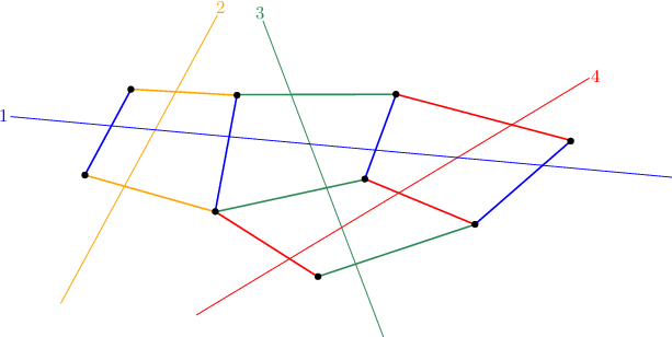
The color classes of a partial cube representing the tope graph of a realizable COM can be determined straightforwardly: all edges corresponding to the same hyperplane belong to the same color class. This is visualized in Fig. 3 for our COM from Fig. 1. In this case, the complementary halfspaces correspond to the sets of vertices on either side of the hyperplane.

More generally, the color classes of a partial cube group together edges corresponding to changes in the same bit of the binary strings in the underlying hypercube. One of the complementary halfspaces consist of all vertices that have a value of $1$ at a specific bit and the other of the vertices that have a value of $0$.

A partial cube minor (pc-minor) is obtained by either contracting an entire color class or restricting the graph to one of its half spaces. It represents a specific type of classical graph minor. For the realizable COM shown in Fig. 1, the different ways for deriving a pc-minor are illustrated in Fig. 4.

Let us now define the class of forbidden pc-minors, that characterize COMs.

For $n=4$ some of the forbidden pc-minors are demonstrated in Fig. 5.

Knauer and Marc [7, Theorem 1.1] proved the following:

Since the tope graph of a COM determines it completely up to orientation, the theorem means that COMs can be characterized as partial cubes that do not contain a forbidden pc-minor.

To summarize, forbidden pc-minors provide a clear criterion for distinguishing COMs among partial cubes. As we aim to explore the Varchenko determinant of partial cubes beyond COMs, these minors serve as natural candidates for investigation, offering minimal examples of non-COM structures.

We start by defining the Varchenko matrix of a COM:

The Varchenko matrix of the realizable COM $\mathcal{M}$ from Fig. 1 is

In [5], the authors showed that the determinant of the Varchenko matrix of a COM has a structured factorization formula:

We observe that, instead of indexing the variables in the monomials of the individual factors by intersections of hyperplane arrangements, we now have zero sets of covectors. This correspondence becomes especially clear in the realizable case. For the Varchenko matrix of the COM in Fig. 1 we computed the determinant and get

which is in line with Theorem 4.0.

The Varchenko matrix can be easily generalized to partial cubes by substituting the role of the topes with vertices and defining the separator $S(u,v)$ of two vertices $u$ and $v$ by the color classes we have to cross on a shortest path between two vertices.

Let us demonstrate this on the forbidden pc-minor $Q_{4}^{--}(4)$. The color classes of this partial cube are illustrated in Fig. 6 together with the assumed linear order of the vertices. We will use $x_{1}$ for the yellow color class, $x_{2}$ for the red one and $x_{3}$, $x_{4}$ for green and blue respectively.

We get the following Varchenko matrix for $Q_{4}^{--}(4)$:

The question of whether the generalized Varchenko determinant retains a clean factorization, i.e. the factors look like in (1), beyond COMs has been answered negatively in [5] by examining $Q_{4}^{--}(4)$, as

where the last factor is obviously not in the form of (1). This leads to another question: Does the Varchenko matrix of a partial cube factorize nicely if and only if it is the tope graph of a COM? This question can also be answered negatively by looking at the Varchenko determinant of $Q_{4}^{--}(1)$. The color classes of that partial cube together with the linear order of the vertices are also illustrated in Fig. 3.

For this matrix we get

where each factor is in the form of (1). This observation raises the concluding question of whether partial cubes with a well-structured Varchenko determinant can be characterized by other distinct properties.

In this paper, we generalized the Varchenko matrix to partial cubes and observed its determinant. Although the Varchenko matrix admits a clean factorization when the partial cube is the tope graph of a COM, this property does not hold in general, as illustrated by a known example of a minimal non-COM partial cube. We answered the question whether the Varchenko determinant has a nice factorization if and only if the partial cube is the tope graph of a COM negatively: by examining the determinants of other partial cubes that are forbidden pc-minors for COMs, we found one that still admits a clean factorization. This raises the question of whether partial cubes with a nice Varchenko determinant factorization can be characterized in another way. If this question can be answered, it would be very interesting to know to what structural property the indices of the monomials in the factorization belong.

To feed the intuition for further research on Varchenko determinants of partial cubes, we provide a summary of all the determinants we tested below. We used Python and Maple for our computations. In order to check if a graph is a partial cube and determine its color classes, we used the work of David Eppstein [3] together with the corresponding code https://ics.uci.edu/~eppstein/PADS/. The Python code that generates the Varchenko matrix of a partial cube can be found here:

https://github.com/SophiaKeip/VarchenkoMatrixPartialCubes.

Note that the color classes and vertices in the code are numbered differently from those in the examples above. The numbering in the examples was chosen for illustrative purposes.

Varchenko determinants for $n=4$:

Varchenko determinants for $n=5$:

References

• [1] Hans-Jürgen Bandelt, Victor Chepoi, and Kolja Knauer. Coms: complexes of oriented matroids. Journal of Combinatorial Theory, Series A, 156:195–237, 2018.
• [2] D Ž Djoković. Distance-preserving subgraphs of hypercubes. Journal of Combinatorial Theory, Series B, 14(3):263–267, 1973.
• [3] David Eppstein. Recognizing partial cubes in quadratic time. arXiv preprint arXiv:0705.1025, 2007.
• [4] Regina Gente. The varchenko matrix for cones. 2013.
• [5] Winfried Hochstättler, Sophia Keip, and Kolja Knauer. The signed varchenko determinant for complexes of oriented matroids. Combinatorica, 45(2):19, 2025.
• [6] Winfried Hochstättler and Volkmar Welker. The varchenko determinant for oriented matroids. Mathematische Zeitschrift, 293:1415–1430, 2019.
• [7] Kolja Knauer and Tilen Marc. On tope graphs of complexes of oriented matroids. Discrete & Computational Geometry, 63(2):377–417, 2020.
• [8] Hery Randriamaro. The varchenko determinant of an oriented matroid. arXiv preprint arXiv:2003.01970, 2020.
• [9] Hery Randriamaro. The varchenko matrix for topoplane arrangements. Communications in Contemporary Mathematics, 24(10):2150086, 2022.
• [10] Alexandre Varchenko. Bilinear form of real configuration of hyperplanes. Adv. Math, 97(1):110–144, 1993.
• [11] Peter M Winkler. Isometric embedding in products of complete graphs. Discrete Applied Mathematics, 7(2):221–225, 1984.