Utilizing Strategic Pre-training to Reduce Overfitting: Baguan - A Pre-trained Weather Forecasting Model

Abstract.
Weather forecasting has long posed a significant challenge for humanity. While recent AI-based models have surpassed traditional numerical weather prediction (NWP) methods in global forecasting tasks, overfitting remains a critical issue due to the limited availability of real-world weather data spanning only a few decades. Unlike fields like computer vision or natural language processing, where data abundance can mitigate overfitting, weather forecasting demands innovative strategies to address this challenge with existing data. In this paper, we explore pre-training methods for weather forecasting, finding that selecting an appropriately challenging pre-training task introduces locality bias, effectively mitigating overfitting and enhancing performance. We introduce Baguan, a novel data-driven model for medium-range weather forecasting, built on a Siamese Autoencoder pre-trained in a self-supervised manner and fine-tuned for different lead times. Experimental results show that Baguan outperforms traditional methods, delivering more accurate forecasts. Additionally, the pre-trained Baguan demonstrates robust overfitting control and excels in downstream tasks, such as subseasonal-to-seasonal (S2S) modeling and regional forecasting, after fine-tuning.
Keywords:
Pre-training, Over-fitting, Vision Transformer, Siamese Masked Autoencoders, Medium-range Weather Forecasting1. Introduction
Data-driven weather forecasting models have significantly advanced the boundaries of meteorological science (Lam et al., 2023; Bi et al., 2023; Chen et al., 2023c; Chen et al., 2023a). These advanced models are typically trained on the ERA5 dataset (Hersbach et al., 2020), produced by the European Centre for Medium-Range Weather Forecasts (ECMWF). Notably, these approaches have consistently outperformed traditional numerical weather prediction (NWP) techniques in both accuracy in standard forecast metrics and inference speeds for operational use (Rasp et al., 2024; Shi et al., 2025). However, as data-driven models grow in scale, the risk of overfitting becomes a significant concern. Unlike fields such as Computer Vision (CV) and Natural Language Processing (NLP) which benefit from the availability of large scale datasets, weather forecasting is constrained by limited real-world data, exemplified by the ERA5 dataset, which spans only a few decades (Hersbach et al., 2020).
| Method | Pangu(Bi et al., 2023) | FuXi(Chen et al., 2023c) | GraphCast (Lam et al., 2023) | FengWu (Chen et al., 2023a) | FCN (Kurth et al., 2023) | Aurora (Bodnar et al., 2024) | Climax (Nguyen et al., 2023a) | Prithvi (Schmude et al., 2024) | Ours: MAE (He et al., 2022b; Man et al., 2023) | Ours: Siamese MAE |
| Pre-training Used | ![[Uncaptioned image]](2505.13873v1/figures/cha.png) |
|
|
|
|
![[Uncaptioned image]](2505.13873v1/figures/gou.png) |
|
|
|
|
| Impact of Pre-training | - | - | - | - | - | Positive | Positive | Negative | Mildly Positive | Positive |
| Free of Additional Data | |
|
|
|
|
|
|
|
|
|
In weather forecasting, overfitting is often linked to inaccurate interactions. The vast input size, which encompasses the entire Earth, can cause the model to learn arbitrary relationships, especially when global attention mechanisms are employed. Beyond augmenting training data, such as introducing extensive climate simulation datasets (Bodnar et al., 2024), researchers have pursued two main strategies to address this issue. The first strategy involves designing models that incorporate locality bias, such as those based on CNNs (Cheon et al., 2024), GNNs (Lam et al., 2023; Lang et al., 2024), or local attention mechanisms (Zhong et al., 2024; Chen et al., 2023a; Bi et al., 2023). These models have been thoroughly explored in the context of weather forecasting. The second strategy focuses on using pre-training tasks to introduce locality bias into models, which generally offers more adaptability and flexibility than the model design approach. However, it is surprising that the effectiveness of this method has been largely underreported in previous research, with the exception of a few studies (Man et al., 2023; Nguyen et al., 2023a). Notably, most widely used weather forecasting models only utilize the prediction task as their primary focus, essentially treating it as a pre-training task (Nguyen et al., 2023a; Bodnar et al., 2024). They do not employ an independent pre-training stage to enhance the subsequent forecasting task. We believe the community might have attempted this approach and encountered challenges or mixed results. As highlighted in (Schmude et al., 2024), the MAE pre-training stage significantly hinders subsequent weather forecasting performance. In contrast, (Man et al., 2023) documents a positive impact of MAE. Our experiments reveal a subtle yet positive enhancement in downstream weather forecasting tasks, though this improvement might be easily overlooked when utilizing a simplistic MAE pre-training method. This may explain why few weather forecasting models utilize an independent pre-training stage as shown in Table 1. Given that the pre-training stage is model-agnostic, we believe this approach holds significant potential for controlling overfitting without altering the model design. It is also highly applicable to downstream tasks due to its simplicity and flexibity.
In this paper, we explore pre-training as a means to mitigate overfitting in weather forecasting models as shown in Fig. 1(a). We focus on Masked Image Modeling (MIM) (He et al., 2022b; Xie et al., 2022; Gupta et al., 2023) for weather data, recognizing the complexity of weather signals compared to images or videos, which makes MAE less effective. To tackle this, we use a Siamese MAE framework that introduces additional signals to gradually adjust pre-training difficulty (formally defined in Eq. 5), employing a dual objective of recovery and prediction tasks, as illustrated in Fig. 1(b). Our approach, detailed through multi-stage tuning and comparative analyses with models like ClimaX (Nguyen et al., 2023a), shows that pre-training significantly enhances overfitting control, particularly in climate-related tasks with limited data. And the effective control of overfitting is achieved by introducing a relatively strong local inductive bias through a model-agnostic design, as illustrated in Fig. 1(c).
Building upon the analysis of pre-training, we introduce Baguan, a Transformer-based model that leverages a pre-training fine-tuning paradigm with Siamese MAE. Due to the comprehensive training on vast datasets, Baguan emerges as an ideal foundational model for diverse downstream tasks. Beyond the global weather forecasting task, two prominent applications that leverage Baguan as their base model include sub-seasonal to seasonal (S2S) climate forecasting (Vitart and Robertson, 2018; Guo et al., 2024) and regional fine-scale forecasting. Our contributions can be summarized as follows:
- (1)
We conduct an in-depth study on pre-training methods to evaluate their impacts on global weather forecasting, particularly controlling overfitting and analyzing the link between task difficulty and performance. The results demonstrate that our Siamese MAE surpasses the standard MAE and forecasting-based pre-training methods through effectively tuning task difficulty.
- (2)
We present Baguan, which excels in medium-range global forecasting tasks and outperforms both Pangu-Weather and IFS by utilizing a three-stage tuning process and a rolling-based forecasting method.
- (3)
Baguan showcases its capability as a foundational model for a range of downstream tasks. It achieves SOTA performance in S2S forecasting, surpassing ECMWF-S2S, while also delivering robust results in high-resolution regional forecasting within real-world, industry-level weather application systems.
2. Related Work
Deep global models leverage a data-driven approach to learn the medium-range spatiotemporal relationships among atmospheric variables. Within this context, two primary frameworks have gained significant attention: the Graph Neural Networks (GNN) family and the Transformers family. The GNN family, which includes models such as GraphCast (Lam et al., 2023) and AIFS (Lang et al., 2024), represents the Earth’s surface as an irregular and uniformly spaced grid instead of a regular rectangular grid. This innovative representation enables more flexible and efficient modeling of the Earth’s complex geometry. In the Transformer family, ClimaX (Nguyen et al., 2023a) and Stormer (Nguyen et al., 2023b) originate from the standard Vision Transformer (ViT). ClimaX, in particular, introduces a pre-training framework on climate simulation data. Additionally, models such as Pangu-Weather (Bi et al., 2023), FuXi (Chen et al., 2023c), and FengWu (Chen et al., 2023a) leverage the advantages of the Swin Transformer, which effectively captures local features and optimizes memory usage.
Since most deep weather forecasting models leverage ViT, the latest advancements in CV can provide valuable inspiration and insights. Within the field of CV, masked image modeling has seen rapid development. MAE (He et al., 2022b) and SimMIM (Xie et al., 2022) are two notable approaches that involve masking or corrupting a specific portion of information within an image. The model is then tasked with recovering this masked portion, thereby promoting the learning of valuable image representations. Siamese MAE (Gupta et al., 2023) introduces the MAE method for video modeling by incorporating two frames and masking a substantial portion of information in the second frame. Additionally, (Amos et al., 2024) has demonstrated that the integration of data-driven priors through pre-training is crucial for achieving reliable performance estimation in a cost-effective manner.
3. Methodology

3.1. Problem Formulation
Baguan is an advanced data-driven framework designed to generate accurate global medium-range weather forecasts. Baguan takes as input the atmospheric state at time , represented as . denotes the number of atmospheric variables considered in the input, while and represent height and width, respectively. In practical scenarios with a spatial resolution of , and for the Earth. Baguan aims to establish the mapping:
| (1) |
where denotes time interval (6 hours). In fact, Baguan produces 6-hourly forecasts in an autoregressive manner: , where indicates the number of rolling steps. In this way, it can make prediction extending up to a maximum of 7 days.
3.2. The Architecture of Baguan
Fig. 2 provides an overview architecture of Baguan. Baguan is a Siamese MAE pre-trained through a self-supervised learning paradigm. Its architecture consists of a variable aggregation tokenization module, a ViT-like encoder, and a cross-self decoder. A details model configure can be found in Appendix Table 4.
3.2.1. Variable Aggregation & Tokenization
Unlike images, which typically consist of three channels, atmospheric states often encompass more than seventy variables, which presents significant challenges. Therefore, we employ a weather-specific embedding (Nguyen et al., 2023a; Nguyen et al., 2023b) instead of the standard patch embedding used in ViT. The specific weather embedding module is composed of a variable aggregation module and a tokenization module. Their objective is to transform the image-like input into a sequence of tokens.
In the variable aggregation module, the input tensor is processed through a series of variable-specific embedding layers, resulting in a tensor of shape . Subsequently, a cross-attention mechanism is employed, utilizing a learnable query with dimensions to aggregate the embedded tensor into a tensor of shape .
In the variable tokenization module, a patchify method is applied to convert this aggregated tensor into a sequence of tokens with shape , where is patch size.
3.2.2. Encoder
In the encoder, the tokens generated by the initial state at time and the target state at time are subsequently processed by a stack of Transformer blocks, producing output tokens denoted as and . The encoder employs the standard ViT architecture. During the pre-training stage, the initial state remains unmasked, whereas the target state is partially masked with Gaussian noise with a ratio of 75%. In contrast, during the fine-tuning and inference stages, the target state is replaced by pure Gaussian noise. Additionally, lead time embedding and positional embedding are incorporated into the tokens to provide contextual information. Notably, the two input frames share the same encoder weights, enabling the model to learn shared representations across both inputs.
3.2.3. Decoder
The decoders used in the pre-training (stage 1) and fine-tuning (stages 2 and 3) processes exhibit slight differences, and the weight of the decoder in pre-training will not be carried over to the fine-tuning stages. The purpose of pre-training is to slowly reconstruct with limited cues, while fine-tuning is aimed at forecasting without any cues, based solely on the initial state . Therefore, we employ two distinct decoders during the pre-training and fine-tuning stages.
3.2.4. Cross-self Decoder
A cross-self decoder architecture is employed, which consists of a stack of blocks. Each block is composed of a cross-attention layer and a self-attention layer. The entire process can be represented by:
| (2) |
| (3) |
| (4) |
where are the parameter matrices of cross-attention layer and self-attention layer. and are the functions of multi-head attention module and feed-forward networks.
3.2.5. Adaptive Layer Normalization
Adaptive layer normalization (AdaLN) (Peebles and Xie, 2022; Perez et al., 2018) is a widely used technique and has been successfully integrated into weather forecasting (Nguyen et al., 2023b). In this paper, we employ AdaLN, a mechanism where the parameters of the normalization layer are learned from the embedding of in the Transformer blocks rather than traditional additive lead time embedding.
3.3. Three Training Stages of Baguan
As shown in Fig. 2, Baguan undergoes three training stages. Initially, the Siamese MAE is pre-trained on the Siamese masked image modeling (SMIM) tasks. Following this, Baguan is fine-tuned for specific lead times of 1 hour, 6 hours or 24 hours. The final stage involves iterative fine-tuning using multi-step data.
3.3.1. Stage 1: Pre-training with Siamese MAE
Siamese network is a weight-sharing neural network that serves as a crucial element in modern contrastive representation learning methods (Chen and He, 2020). Specifically, we employ the asymmetric masking strategy where no patches (0%) in are masked, and a high ratio (=75%) of patches in are masked. The task difficulty can be adjusted by varying the masking ratio . Notably, the task difficulty is inversely proportional to the number of tokens provided. For two input frames corresponding to time steps and , the task difficulty () during pretraining is described as:
| (5) |
where and denote the information contribution of frames and , respectively, in reconstructing the unmasked tokens. and represents the masking ratios for frames and , respectively. In the case of MAE, we have , whereas for Siamese MAE, .
Both and share the encoder weights and the representations are fed into the decoder to reconstruct . This task simplifies the forecasting process and encourages the model to concentrate on the changes occurring between two input frames.
3.3.2. Stage 2: Fine-tuning on Fixed Lead Time
After being pre-trained on the Siamese masked image modeling task, the Baguan encoder is subsequently fine-tuned using fixed lead times of 1 hour, 6 hours, or 24 hours. In Stage 2, information about is entirely unavailable, resulting in the input for frame 2 being effectively masked at a ratio of 100%. Consequently, the frame 2 relies solely on positional and lead time embeddings.
3.3.3. Stage 3: Iterative Fine-tuning
To enhance Baguan’s multi-step forecasting accuracy and reduce the error accumulation associated with simply rolling the model, we introduce an iterative fine-tuning strategy in Stage 3. This approach leverages an auto-regressive training scheme, where the model’s output at each step is recursively fed back as input for subsequent predictions. Formally, for a given initial state , the prediction at time is computed as:
| (6) | ||||
During the inference stage, the auto-regressive strategy is similarly applied.
3.4. Ensemble Strategy
To deal with uncertainty in initial conditions and error accumulation introduced by longer forecast lead times, ensemble forecasting is commonly used in both traditional numerical weather prediction (Coiffier, 2011) and recently proposed AI-based methods (Chen et al., 2023c; Bi et al., 2023; Kurth et al., 2023). Usually, it incorporates noise into the initial conditions to generate multiple predictions. Recently, Stormer (Nguyen et al., 2023b) proposes a randomized iterative ensemble strategy that combines multiple models, including 6-hour and 24-hour models, to enhance long-term forecasting accuracy. However, its Best in strategy (Nguyen et al., 2023b) still requires a comprehensive search through all combinations. To enhance the pruning of the search space, we propose a novel strategy outlined by the following rules:
- (1)
Combination Rule: We employ various combinations for lead times, such as [6, 6, 6, 6] and [24] for a 24-hour forecasting. The combinations are not restricted to identical lead times. For exmaple, 48 hours can be assembled in various ways, such as using four 6-hour and one 24-hour.
- (2)
Pruning Rule: The extended lead time can lead to an exponential increase in possible combinations. To address this, we implement a filtering mechanism that limits the number of iterations to enhance efficiency and accelerate the inference process.
With this ensemble strategy, Baguan achieves an average improvement of approximately 2% in longer lead-time forecasts, helping to reduce accumulated errors. Appendix A.5 presents the detailed results of the ablation experiments.
3.5. Pre-training as Regularization
In this section, we develop a theoretical framework to explore how pre-training improves downstream task performance. Given the complexity of analyzing large deep learning models, we concentrate on linear regression to demonstrate how pre-training serves as a regularization mechanism, mitigating overfitting. We demonstrate that pre-training effects analogous to pruning the subspace spanned by eigenvectors with small eigenvalues, hence regularizing the final solution to rely primarily on the leading eigenvectors of the covariance matrix. This regularization enhances generalization when the target solution resides within the subspace of leading eigenvectors.
We begin with the standard setup of linear regression. For a set of training examples where and , and a covariance matrix , we consider an optimal weight vector in the subspace spanned by the top eigenvectors of . Our analysis shows that pre-training with a denoising model using self-regression improves generalization performance.
We have the following key findings:
- (1)
Without pre-training, the error bound for the estimated weights, considering the top eigenvectors, is given by:
(7) - (2)
By employing a pre-training method (denoising), with high probability the error bound becomes:
(8)
These findings indicate a significant improvement in the generalization error. Indeed, this analysis is performed on a simplified case, but it justifies our modeling based on pre-training for weather forecasting to some extend. Detailed derivations and proofs supporting these results are provided in Appendix A.12.
4. Experiments
4.1. Experimental Settings
4.1.1. Dataset
We utilize the ERA5 dataset (Hersbach et al., 2020) as the ground truth for model training and inferencing. Produced by the European Centre for Medium-Range Weather Forecasts (ECMWF), ERA5 is a global atmospheric reanalysis dataset providing detailed information on the Earth’s climate and weather conditions from 1940 to the present. It includes a wide range of variables, such as temperature, humidity, precipitation, and mean sea level pressure, etc. This dataset is available at a high spatial resolution of latitude-longitude, roughly equivalent to approximately 31 kilometers, and encompasses 37 vertical pressure levels. As detailed in Appendix A.1, we select a subset of 13 of these levels (50 hPa, 100 hPa, 150 hPa, 200 hPa, 250 hPa, 300 hPa, 400 hPa, 500 hPa, 600 hPa, 700 hPa, 850 hPa, 925 hPa, 1000 hPa), along with four surface variables (2m temperature, u-component and v-component of 10m wind speed, and mean sea level pressure) and several statistic variables. Following Pangu-Weather (Bi et al., 2023), we use the data from 1979 to 2015 for training, 2016 to 2017 for validation, and 2018 for testing. Same as Pangu-Weather, our training stages involve using 1-hourly data, rather than 6-hourly in FuXi (Chen et al., 2023b) and FengWu (Chen et al., 2023a). During testing, forecasts are initialized at 00 and 12 UTC, a standard benchmark time for comparing forecast scores across weather forecasting models (Rasp et al., 2024).
4.1.2. Implementation Details
The size of the input data from ERA5 is . During the tokenization stage, we employ a patch size of , which results in 16380 tokens. Baguan consists of encoders with a depth of 16, and a hidden dimension of 2048, as well as decoders with a depth of 4 and hidden dimension of 1024 both for pre-training and fine-tuning. A batch size of 1 is employed on each GPU. The model configuration and details of each stage can be found in Appendix A.4 and Appendix A.3. Furthermore, we intend to open-source the checkpoint along with all training and evaluation codes, believing it will serve as a valuable baseline for the community.
4.1.3. Evaluation Metrics & Training Objective
Following prior work (Bi et al., 2023; Lam et al., 2023), two specific quantitative metrics are employed to assess the accuracy of forecasting: the Latitude-Weighted Root Mean Square Error (RMSE) and the Latitude-Weighted Anomaly Correlation Coefficient (ACC).
For optimization, we use the Mean Square Error (MSE) loss for pre-training and Mean Absolute Error (MAE) loss for fine-tuning. More details can be found in Appendix A.2.
4.2. The Effectiveness of Siamese MAE Pre-training
4.2.1. Empirical Comparison of Pre-training Approaches
To evaluate the effectiveness of different pre-training approaches, we conducted a comparison between Siamese MAE (Gupta et al., 2023) and MAE (He et al., 2022a). The without pre-train version served as a baseline to normalize the results (RMSE) obtained from both Siamese MAE and MAE pre-training. Among these pre-training tasks, the w/o pre-train version presents the most challenging scenario, as it has no information regarding the second frame. In contrast, the MAE focuses on reconstructing the current frame while preserving 25% of the patches. The Siamese MAE, on the other hand, represents the simplest task, as it utilizes information from both the current and 25% of the second frames.
Fig. 3 (Left) provides the results using the resolution data for 6-hour prediction. The results indicate that Baguan, when utilizing Siamese MAE pre-training, outperforms the w/o pre-training version by an average improvement of 10.1% in RMSE across four key variables. In contrast, Baguan with standard MAE pre-training achieves only a 4.5% average improvement over the w/o pre-training version, underscoring the superior effectiveness of the Siamese MAE approach.
The primary purpose of introducing pre-training is to mitigate overfitting, as discussed earlier in Fig. 1(a). To quantify this effect, we calculate the mean MSE over the last 50 training steps. The pre-trained model exhibits a train-validation loss gap of , compared to for the non-pre-trained model, underscoring the role of pre-training in reducing overfitting.
4.2.2. Spectrum Analysis of Learned Representations
In Sec 3.5, our theoretical analysis demonstrates that pre-training mitigate overfitting by regularizing the solution to rely on leading eigenvectors of the covariance matrix.
For Baguan, a deep transformer model, we assume that the attention map functions similarly to the covariance matrix in a linear regression model. Based on this assumption, we perform spectral analyses on the attention scores associated with the center token in the map. Since there are a total of around 16,000 tokens, there are around 16,000 attention scores corresponding to this particular token. We observe that the energy of the leading eigenvectors is higher in the pre-trained model compared to the non-pre-trained model. We present the results in Fig. 4. Through this experiment, we aim to uncover the underlying mechanism of how pre-training operates, both from theoretical and empirical perspectives.
4.2.3. Attention Map Visualization
Fig. 1(c) illustrates the attention maps for the center token in the map for both the Siamese MAE and MAE in the layer, within a total of 16 layers. The attention map of Siamese networks exhibits a stronger locality with lower-rank characteristics, effectively suppressing overfitting. This stronger locality implies that the attention map is more concentrated, with higher energy observed in the leading eigenvectors when viewed in the spectral domain. This phenomenon offers evidence for the conclusion in Section 3.5 that pre-training mitigates overfitting by pruning the subspace spanned by eigenvectors with small eigenvalues.
Specifically, when the attention values exceed a certain threshold, they are considered activated by the current token. In this context, 0.25% of tokens are activated by Siamese MAE, while 1.61% of tokens are activated more than six times by MAE. Furthermore, the attention maps presented correspond to a 6-hour forecast, which is typically characterized by a relatively localized impact. However, MAE has activated nearly all tokens along the entire equator, indicating an unusually broad response. This discrepancy is more likely indicative of an overfitting issue of MAE rather than an actual long-term effect on weather forecasting. A more detailed visualization of the attention maps can be found in Appendix A.8.
4.2.4. Ablation on Masking Ratio
We conduct experiments to compare the effects of task difficulty by varying different masking ratios using the resolution data for 6-hour prediction. It is important to note that a higher masking ratio corresponds to a more challenging pre-training task, making it increasingly similar to the w/o pre-training task. As shown in Fig. 3 (Right), the Siamese MAE with masking ratios of 0.75, 0.95, and 0.99 achieves average improvements of 8.4%, 8.8%, and 8.4% in RMSE on key variables, respectively, compared to the w/o pre-training version. While we observe optimal performance at a masking ratio of 0.95, increasing the masking ratio, particularly at 0.95 and 0.99, the pre-training process becomes unstable, characterized by significant spikes in the training loss. Consequently, to make a stable pre-training performance, we tend to choose a relative smaller masking ratio (e.g., 0.75) in our experiment.
4.3. Weather Forecasting Tasks on ERA5 Dataset
In Fig. 5, we present a comprehensive evaluation of Baguan (depicted by green lines), in comparison with Pangu-Weather and IFS models. The test set utilizes data from the year 2018 at 00 and 12 UTC. We compare the RMSE and ACC across lead times ranging from 1 hour to 7 days. Baguan demonstrates a lower RMSE than Pangu-Weather for 75.2% of the key variables, with an average improvement of 4.7%. Notably, for key variables such as T2M and U10, Baguan outperforms Pangu-Weather with average improvements of 4.0% and 7.8%, respectively
Additionally, Baguan consistently outperforms IFS, achieving an average improvement of 23.2%. In particular, for T2M, Baguan results in an average enhancement of 28.3%. As the lead time increases, the magnitude of our improvement becomes even more evident.
Our goal is to thoroughly study the effectiveness of pre-training using a simple ViT-based architecture without model-specific locality design. We did not compare our results with models (Chen et al., 2023c; Lam et al., 2023; Chen et al., 2023a), as they mainly use GNNs or local attention mechanisms to induce locality and also we lack training codes for these algorithms to make a fair comparison. Future work will explore combining model-specific locality with pre-training-induced locality to collaboratively address the overfitting issue to make more accurate forecast.
4.4. Baguan as Foundation Model
4.4.1. Baguan for S2S
Weather and climate forecasting covers a wide range of timescales. In addition to predicting weather conditions within the medium-range, subseasonal to seasonal (S2S) forecasting (2 to 6 weeks ahead) (Vitart and Robertson, 2018) also holds significant value in terms of disaster preparedness, such as droughts and floods. By fine-tuning Baguan with a novel multi-stage optimization approach, (Guo et al., 2024) demonstrates an impressive achievement in the S2S task. Their results outperform SOTA NWP systems(ECMWF-S2S), as illustrated in Fig. 6. Recent benchmark work (Nathaniel et al., 2024) indicates that most deep learning models have shown weaker performance compared to ECMWF-S2S.
Additionally, Fig. 6(a) presents an analysis of overfitting among Baguan-P (pre-training), Baguan-S (train from scratch), and FuXi, a model based on the Swin Transformer architecture. Despite observing a low training loss with FuXi (0.38) and a higher training loss with Baguan (0.60), the Baguan-P model achieves significantly better validation accuracy, improving the TCC value by over 25%, from 0.265 to 0.337, compared to its w/o pre-training counterpart. This underscores Baguan-P’s capability to mitigate overfitting through pre-training. We argue that in long-term subseasonal forecasting, where the signal-to-noise ratio is low, the risk of overfitting becomes more severe. In this context, Baguan’s ability to address overfitting is particularly evident.

4.4.2. Baguan for Regional Forecasting
Regional forecasting achieving kilometer-scale predictions is vital for applications such as risk assessment and understanding local effects (Mardani et al., 2023). To enhance the precision of these forecasts, we have advanced beyond the traditional resolution of the ERA5 dataset by introducing a finer regional dataset with a resolution of . By incorporating an additional encoder to process the tokens from this high-resolution regional analysis data and integrating them with global tokens, Baguan outperforms simple interpolation to high resolution. The forecasting system has been deployed to assist the electricity sector in an eastern province of China, covering over 1.5 million square kilometers and impacting 100 million people.
We perform short-term regional forecasting experiments utilizing data from the China Meteorological Administration Land Data Assimilation System (CLDAS). This dataset features grid spacing across China (16-54°N, 74-134°E) for the years 2022 and 2023, using the first one and a half years for training and the remaining half year for testing. As results shown in Table 2, we compare the regional forecasting outcomes of EC-IFS, Baguan-Interpolation (which interpolates the forecasts from the foundation model), and Baguan-Regional (which includes an additional encoder for regional analysis data). Baguan-Regional demonstrates significantly superior performance compared to EC-IFS, achieving an average improvement of 57.8% on key variables in regional forecasting. Baguan can be fine-tuned on variables not present in the pre-trained dataset, making it highly suitable for real-world applications. Additionally,it outperforms naive interpolation by an average of 47.0% on the same variables. These results highlight Baguan’s enhanced forecasting capabilities at higher resolutions, achieved with only minimal adjustments. A more comprehensive description and detailed results can be found in Appendix A.10.
| Variable | Lead | EC-IFS | Baguan- | Baguan- | |
| time | Interpolation | Reigional | |||
| 6h | 2.04 | 2.29 | 1.38 | ||
| 24h | 2.05 | 2.36 | 1.63 | ||
| 6h | 4.51 | 3.95 | 1.33 | ||
| 24h | 4.82 | 4.60 | 2.26 |
4.5. Pre-Training Across Diverse Scales
4.5.1. Model Scaling Analysis
In Fig. 7 (Left), we evaluate the scaling laws for models with and without pre-training, revealing three key findings as follows. (1) Pre-training demonstrates greater effectiveness for larger models (+4.20% -> +10.1% at and +6.02% -> 8.03% at ), suggesting that the benefits of pre-training scale with model capacity. (2) Model performance increases with model size, but saturates as the model reaches a sufficient scale. (3) Our analysis underscores the critical role of data resolution in model performance. Higher resolution inputs, which inherently contain more tokens, consistently lead to improved results. Notably, increasing the data resolution to reduces the validation MSE by 74.0% and 38.8% compared to resolutions of and , respectively.
4.5.2. Data Scaling Analysis
Fig. 7 (Right) illustrates the empirical relationship between data scale and model performance. As discussed in previous sections, the constrained temporal scale of the ERA5 dataset (40 years) presents a fundamental limitation, resulting in model overfitting. Our experimental results substantiate this finding: while training loss consistently converges to similar levels across different dataset sizes, validation loss deteriorate with reduced data volume. This suggests that smaller datasets, due to their limited diversity in representing Earth’s atmospheric states, consistently result in poorer generalization performance.The utilization of a 40-year dataset demonstrates average improvements of 27.4%, 8.9%, and 2.1% over datasets spanning 2 years, 6 years, and 20 years, respectively. Furthermore, among the four key variables analyzed, z500 exhibits the highest susceptibility to overfitting compared to the other three variables.
4.6. Visualization
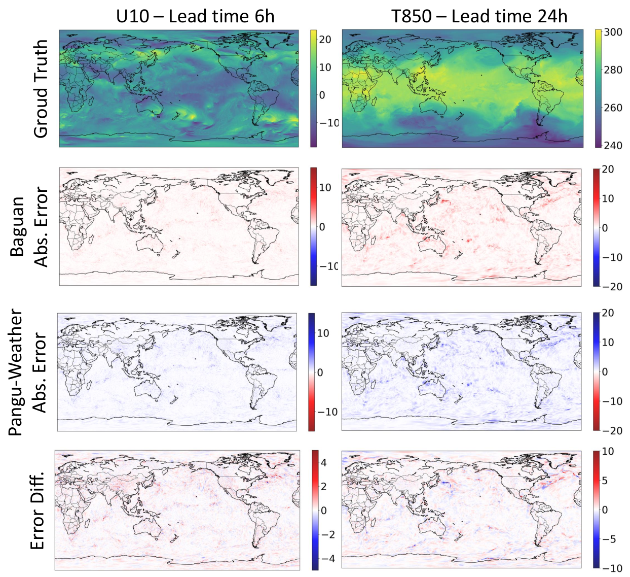
Fig. 8 illustrates the spatial distributions of absolute error for Baguan and Pangu-Weather at lead times of 6 hours and 24 hours. The initial state is set for January 1, 2018, at 00:00 UTC. The locations with discrepancies on the map are more apparent in Pangu-Weather. Additionally, We visualize the difference in absolute error between Baguan and Pangu-Weather. The results indicate that a greater portion (73% for U10 and 58% for T850) of the spatial map is red, suggesting that our Baguan model performs better.
5. Conclusion and Future Work
Conclusion
In this paper, we introduce Baguan, an advanced data-driven system designed to push the boundaries of weather forecasting. Our work delivers three major technical contributions: (1) We conduct a systematic investigation into pre-training techniques to effectively mitigate overfitting and enhancing the model’s generalizability and robustness. (2) Baguan demonstrates superior performance, outperforming IFS and Pangu-Weather across a range of benchmarks. (3) We show that Baguan excels in various downstream tasks, including S2S and regional forecasting, showcasing its versatility and applicability across different temporal and spatial scales in meteorological prediction.
Future Work
In the future, we will continue to explore and conduct research from multiple perspectives, including: (1) We aim to investigate larger model architectures, employing advanced pre-training techniques to enhance the model’s robustness and performance. (2) For downstream tasks, we aim to apply Baguan to a broader range of meteorological applications, including extreme weather forecasting and climate prediction. Appendix. A.11 presents an initial attempt at tracking tropical cyclones using Baguan. (3) To meet the diverse needs of our users, we will develop a modular system allowing users to select specific functional components and provide more flexible deployment options, ensuring better adaptability to different operational environments.
References
- Amos et al. (2024) Ido Amos, Jonathan Berant, and Ankit Gupta. 2024. Never Train from Scratch: Fair Comparison of Long-Sequence Models Requires Data-Driven Priors. In The Twelfth International Conference on Learning Representations, ICLR 2024, Vienna, Austria, May 7-11, 2024. OpenReview.net. https://openreview.net/forum?id=PdaPky8MUn
- Bi et al. (2023) Kaifeng Bi, Lingxi Xie, Hengheng Zhang, Xin Chen, Xiaotao Gu, and Qi Tian. 2023. Accurate medium-range global weather forecasting with 3D neural networks. Nature 619, 7970 (2023), 533–538.
- Bodnar et al. (2024) Cristian Bodnar, Wessel P. Bruinsma, Ana Lucic, Megan Stanley, Johannes Brandstetter, Patrick Garvan, Maik Riechert, Jonathan A. Weyn, Haiyu Dong, Anna Vaughan, Jayesh K. Gupta, Kit Thambiratnam, Alex Archibald, Elizabeth Heider, Max Welling, Richard E. Turner, and Paris Perdikaris. 2024. Aurora: A Foundation Model of the Atmosphere. ArXiv abs/2405.13063 (2024). https://api.semanticscholar.org/CorpusID:269983273
- Chen et al. (2023a) Kan Chen, Tao Han, Junchao Gong, Lei Bai, Fenghua Ling, Jingyao Luo, Xi Chen, Lei Ma, Tianning Zhang, Rui Su, Yuanzheng Ci, Bin Li, Xiaokang Yang, and Wanli Ouyang. 2023a. FengWu: Pushing the Skillful Global Medium-range Weather Forecast beyond 10 Days Lead. ArXiv abs/2304.02948 (2023). https://api.semanticscholar.org/CorpusID:257985330
- Chen et al. (2023b) Lei Chen, Xiaohui Zhong, Feng jun Zhang, Yuan Cheng, Yinghui Xu, Yuan Qi, and Hao Li. 2023b. FuXi: a cascade machine learning forecasting system for 15-day global weather forecast. npj Climate and Atmospheric Science 6 (2023), 1–11. https://api.semanticscholar.org/CorpusID:259224665
- Chen et al. (2023c) Lei Chen, Xiaohui Zhong, Feng Zhang, Yuan Cheng, Yinghui Xu, Yuan Qi, and Hao Li. 2023c. FuXi: a cascade machine learning forecasting system for 15-day global weather forecast. npj Climate and Atmospheric Science 6, 1 (2023), 190. https://doi.org/10.1038/s41612-023-00512-1
- Chen and He (2020) Xinlei Chen and Kaiming He. 2020. Exploring Simple Siamese Representation Learning. 2021 IEEE/CVF Conference on Computer Vision and Pattern Recognition (CVPR) (2020), 15745–15753. https://api.semanticscholar.org/CorpusID:227118869
- Cheon et al. (2024) Minjong Cheon, Yo-Hwan Choi, Seon-Yu Kang, Yumi Choi, Jeong-Gil Lee, and Daehyun Kang. 2024. Karina: An efficient deep learning model for global weather forecast. arXiv preprint arXiv:2403.10555 (2024).
- Coiffier (2011) Jean Coiffier. 2011. Fundamentals of numerical weather prediction. Cambridge University Press.
- Guo et al. (2024) Yizhen Guo, Tian Zhou, Wanyi Jiang, Bo Wu, Liang Sun, and Rong Jin. 2024. Maximizing the Impact of Deep Learning on Subseasonal-to-Seasonal Climate Forecasting: The Essential Role of Optimization. arXiv preprint arXiv:2411.16728 (2024).
- Gupta et al. (2023) Agrim Gupta, Jiajun Wu, Jia Deng, and Fei-Fei Li. 2023. Siamese masked autoencoders. Advances in Neural Information Processing Systems 36 (2023), 40676–40693.
- He et al. (2022a) Kaiming He, Xinlei Chen, Saining Xie, Yanghao Li, Piotr Dollár, and Ross Girshick. 2022a. Masked autoencoders are scalable vision learners. In Proceedings of the IEEE/CVF conference on computer vision and pattern recognition. 16000–16009.
- He et al. (2022b) Kaiming He, Xinlei Chen, Saining Xie, Yanghao Li, Piotr Dollár, and Ross B. Girshick. 2022b. Masked Autoencoders Are Scalable Vision Learners. In IEEE/CVF Conference on Computer Vision and Pattern Recognition, CVPR 2022, New Orleans, LA, USA, June 18-24, 2022. IEEE, 15979–15988. https://doi.org/10.1109/CVPR52688.2022.01553
- Hersbach et al. (2020) Hans Hersbach, Bill Bell, Paul Berrisford, Shoji Hirahara, András Horányi, Joaquín Muñoz-Sabater, Julien Nicolas, Carole Peubey, Raluca Radu, Dinand Schepers, et al. 2020. The ERA5 global reanalysis. Quarterly Journal of the Royal Meteorological Society 146, 730 (2020), 1999–2049.
- Kurth et al. (2023) Thorsten Kurth, Shashank Subramanian, Peter Harrington, Jaideep Pathak, Morteza Mardani, David Hall, Andrea Miele, Karthik Kashinath, and Anima Anandkumar. 2023. FourCastNet: Accelerating Global High-Resolution Weather Forecasting Using Adaptive Fourier Neural Operators. In Proceedings of the Platform for Advanced Scientific Computing Conference, PASC 2023, Davos, Switzerland, June 26-28, 2023, Axel Huebl, Cristina Silvano, and Timothy Robinson (Eds.). ACM, 13:1–13:11. https://doi.org/10.1145/3592979.3593412
- Lam et al. (2023) Remi Lam, Alvaro Sanchez-Gonzalez, Matthew Willson, Peter Wirnsberger, Meire Fortunato, Ferran Alet, Suman Ravuri, Timo Ewalds, Zach Eaton-Rosen, Weihua Hu, Alexander Merose, Stephan Hoyer, George Holland, Oriol Vinyals, Jacklynn Stott, Alexander Pritzel, Shakir Mohamed, and Peter Battaglia. 2023. Learning skillful medium-range global weather forecasting. Science 382, 6677 (2023), 1416–1421. https://doi.org/10.1126/science.adi2336 arXiv:https://www.science.org/doi/pdf/10.1126/science.adi2336
- Lang et al. (2024) Simon Lang, Mihai Alexe, Matthew Chantry, Jesper Dramsch, Florian Pinault, Baudouin Raoult, Mariana C. A. Clare, Christian Lessig, Michael Maier-Gerber, Linus Magnusson, Zied Ben Bouallègue, Ana Prieto Nemesio, Peter D. Dueben, Andrew Brown, Florian Pappenberger, and Florence Rabier. 2024. AIFS – ECMWF’s data-driven forecasting system. arXiv:2406.01465 [physics.ao-ph] https://arxiv.org/abs/2406.01465
- Man et al. (2023) Xin Man, Chenghong Zhang, Jin Feng, Changyu Li, and Jie Shao. 2023. W-mae: Pre-trained weather model with masked autoencoder for multi-variable weather forecasting. arXiv preprint arXiv:2304.08754 (2023).
- Mardani et al. (2023) Morteza Mardani, Noah D. Brenowitz, Yair Cohen, Jaideep Pathak, Chieh-Yu Chen, Cheng-Chin Liu, Arash Vahdat, Karthik Kashinath, Jan Kautz, and Mike Pritchard. 2023. Generative Residual Diffusion Modeling for Km-scale Atmospheric Downscaling. CoRR abs/2309.15214 (2023). https://doi.org/10.48550/ARXIV.2309.15214 arXiv:2309.15214
- Nathaniel et al. (2024) Juan Nathaniel, Yongquan Qu, Tung Nguyen, Sungduk Yu, Julius Busecke, Aditya Grover, and Pierre Gentine. 2024. Chaosbench: A multi-channel, physics-based benchmark for subseasonal-to-seasonal climate prediction. arXiv preprint arXiv:2402.00712 (2024).
- Nguyen et al. (2023a) Tung Nguyen, Johannes Brandstetter, Ashish Kapoor, Jayesh K. Gupta, and Aditya Grover. 2023a. ClimaX: A foundation model for weather and climate. In International Conference on Machine Learning. https://api.semanticscholar.org/CorpusID:256231457
- Nguyen et al. (2023b) Tung Nguyen, Rohan Shah, Hritik Bansal, Troy Arcomano, Sandeep Madireddy, Romit Maulik, Veerabhadra Kotamarthi, Ian T. Foster, and Aditya Grover. 2023b. Scaling transformer neural networks for skillful and reliable medium-range weather forecasting. CoRR abs/2312.03876 (2023). https://doi.org/10.48550/ARXIV.2312.03876 arXiv:2312.03876
- Peebles and Xie (2022) William S. Peebles and Saining Xie. 2022. Scalable Diffusion Models with Transformers. 2023 IEEE/CVF International Conference on Computer Vision (ICCV) (2022), 4172–4182. https://api.semanticscholar.org/CorpusID:254854389
- Perez et al. (2018) Ethan Perez, Florian Strub, Harm de Vries, Vincent Dumoulin, and Aaron C. Courville. 2018. FiLM: Visual Reasoning with a General Conditioning Layer. In AAAI.
- Rasp et al. (2024) Stephan Rasp, Stephan Hoyer, Alexander Merose, Ian Langmore, Peter Battaglia, Tyler Russel, Alvaro Sanchez-Gonzalez, Vivian Yang, Rob Carver, Shreya Agrawal, Matthew Chantry, Zied Ben Bouallegue, Peter Dueben, Carla Bromberg, Jared Sisk, Luke Barrington, Aaron Bell, and Fei Sha. 2024. WeatherBench 2: A benchmark for the next generation of data-driven global weather models. arXiv:2308.15560 [physics.ao-ph] https://arxiv.org/abs/2308.15560
- Schmude et al. (2024) Johannes Schmude, Sujit Roy, Will Trojak, Johannes Jakubik, Daniel Salles Civitarese, Shraddha Singh, Julian Kuehnert, Kumar Ankur, Aman Gupta, Christopher E Phillips, et al. 2024. Prithvi wxc: Foundation model for weather and climate. arXiv preprint arXiv:2409.13598 (2024). https://openreview.net/forum?id=SyBPtQfAZ
- Shi et al. (2025) Jimeng Shi, Azam Shirali, Bowen Jin, Sizhe Zhou, Wei Hu, Rahuul Rangaraj, Shaowen Wang, Jiawei Han, Zhaonan Wang, Upmanu Lall, Yanzhao Wu, Leonardo Bobadilla, and Giri Narasimhan. 2025. Deep Learning and Foundation Models for Weather Prediction: A Survey. arXiv:2501.06907 [cs.LG] https://arxiv.org/abs/2501.06907
- Vitart and Robertson (2018) Frederic Vitart and Andrew Robertson. 2018. The sub-seasonal to seasonal prediction project (S2S) and the prediction of extreme events. npj Climate and Atmospheric Science 1 (03 2018). https://doi.org/10.1038/s41612-018-0013-0
- Xie et al. (2022) Zhenda Xie, Zheng Zhang, Yue Cao, Yutong Lin, Jianmin Bao, Zhuliang Yao, Qi Dai, and Han Hu. 2022. SimMIM: A Simple Framework for Masked Image Modeling. In International Conference on Computer Vision and Pattern Recognition (CVPR).
- Zhong et al. (2024) Xiaohui Zhong, Lei Chen, Xu Fan, Wenxu Qian, Jun Liu, and Hao Li. 2024. FuXi-2.0: Advancing machine learning weather forecasting model for practical applications. CoRR abs/2409.07188 (2024). https://doi.org/10.48550/ARXIV.2409.07188 arXiv:2409.07188
Appendix A Appendix
A.1. Dataset
As illustrated in Table 3, we employ a subset of 13 pressure levels (50 hPa, 100 hPa, 150 hPa, 200 hPa, 250 hPa, 300 hPa, 400 hPa, 500 hPa, 600 hPa, 700 hPa, 850 hPa, 925 hPa, and 1000 hPa), along with four surface variables (2-meter temperature, u-component and v-component of 10-meter wind speed, and mean sea level pressure), as well as several statistical variables.
| Type | Variable name | Abbrev. | Input | Output | ECMWF ID | Levels |
| Static | Land-sea mask | LSM | 172 | - | ||
| Static | geopotential at surface | - | 162051 | - | ||
| Static | angle of sub gridscale orography | ANOR | 162 | - | ||
| Static | anisotropy of sub gridscale orography | ISOR | 161 | - | ||
| Static | lake cover | CL | 26 | - | ||
| Static | soil type | SOILTYP | 500205 | - | ||
| Single | 2 metre temperature | T2m | 167 | - | ||
| Single | 10 metre U wind component | U10 | 165 | - | ||
| Single | 10 metre V wind component | V10 | 166 | - | ||
| Single | mean sea-level pressure | MSL | 151 | - | ||
| Atmospheric | Geopotential | Z | 129 | 50, 100, 150, 200, 250, 300, | ||
| 400, 500, 600, 700, 850, 925, 1000 | ||||||
| Atmospheric | U wind component | U | 131 | 50, 100, 150, 200, 250, 300, | ||
| 400, 500, 600, 700, 850, 925, 1000 | ||||||
| Atmospheric | V wind component | V | 132 | 50, 100, 150, 200, 250, 300, | ||
| 400, 500, 600, 700, 850, 925, 1000 | ||||||
| Atmospheric | Temperature | T | 130 | 50, 100, 150, 200, 250, 300, | ||
| 400, 500, 600, 700, 850, 925, 1000 | ||||||
| Atmospheric | Specific humidity | Q | 133 | 50, 100, 150, 200, 250, 300, | ||
| 400, 500, 600, 700, 850, 925, 1000 |
The "Type" column categorizes variables as static (non-time-varying) properties, time-varying, single-level (surface) properties, or time-varying atmospheric properties. The "Variable Name" and "Abbrev." columns denote the labels assigned by ECMWF, whereas the "ECMWF ID" column specifies the numerical identifier allocated by the organization. The "Input" and "Output" columns indicate whether a variable functions as an input to or an output from Baguan. Lastly, the "Levels" column details the atmospheric levels included in the dataset.
A.2. Evaluation Metrics & Training Objectives
Evaluation metrics
RMSE is a commonly utilized statistical metric in geospatial analysis and climate science to evaluate the precision of a model’s predictions or estimates over various latitudinal ranges:
| (9) |
The latitude weighting factor is used to account for the differences in surface area represented by various latitudes on a spherical Earth. It is given by:
| (10) |
ACC is the spatial correlation between prediction anomalies relative to climatology and ground truth anomalies relative to climatology:
| (11) |
| (12) |
where climatology is the temporal mean of the ground truth data over the entire test set .
Training objectives
We use the Mean Square Error (MSE) loss for pre-training and Mean Absolute Error (MAE) loss for fine-tuning. Given the large number of variables being predicted, we employ pressure-weighted loss to prioritize the weighting of variables near the surface. These weights are normalized to ensure their total sums to 1. Additionally, to align with the evaluation metrics, latitude-weighting is also incorporated in the training objective.
| (13) |
| (14) |
where is the weight of variable .
| Config | Baguan- | Baguan- | Baguan- |
| Encoder Layers | 16 | 16 | 8 |
| Encoder Embed Dim | 2048 | 1024 | 512 |
| Encoder Heads | 16 | 16 | 16 |
| Decoder Layers | 4 | 4 | 4 |
| Decoder Embed Dim | 1024 | 512 | 256 |
| Decoder Heads | 8 | 8 | 8 |
| Patch Size | 8 | 4 | 2 |
| Masking Ratio | 0.75 | 0.75 | 0.75 |
| Scheduler | Cosine | Cosine | Cosine |
| Optimizer | AdamW | AdamW | AdamW |
| Learning Rate - Stage 1 | 5e-4 | 4e-4 | 2e-4 |
| Warm-up Steps - Stage 1 | 40,000 | 20,000 | 10,000 |
| Max Steps - Stage 1 | 250,000 | 200,000 | 100,000 |
| - Stage 1 | 0.9 | 0.9 | 0.9 |
| - Stage 1 | 0.95 | 0.95 | 0.95 |
| Weight Decay - Stage 1 | 0.05 | 0.05 | 0.05 |
| Batch Size - Stage 1 | 24 | 32 | 64 |
| Batch Size / GPU - Stage 1 | 1 | 4 | 16 |
| Learning Rate - Stage 2 | 2e-5 | 1e-5 | 1e-5 |
| Warm-up Steps - Stage 2 | 10,000 | 10,000 | 10,000 |
| Max Steps - Stage 2 | 70,000 | 60,000 | 40,000 |
| - Stage 2 | 0.9 | 0.9 | 0.9 |
| - Stage 2 | 0.99 | 0.99 | 0.99 |
| Weight Decay - Stage 2 | 1e-5 | 1e-5 | 1e-5 |
| Batch Size - Stage 2 | 8 | 32 | 64 |
| Batch Size / GPU - Stage 2 | 1 | 4 | 16 |
| Learning Rate - Stage 3 | 2e-6 | 2e-7 | 2e-7 |
| Warm-up Steps - Stage 3 | 0 | 0 | 0 |
| Max Steps - Stage 3 | 2,000 | 2,000 | 1,000 |
| - Stage 3 | 0.9 | 0.9 | 0.9 |
| - Stage 3 | 0.99 | 0.99 | 0.99 |
| Weight Decay - Stage 3 | 1e-5 | 1e-5 | 1e-5 |
| Batch Size - Stage 3 | 8 | 32 | 64 |
| Batch Size / GPU - Stage 3 | 1 | 4 | 16 |
A.3. Implementation Details of Each Stage
Baguan undergoes three training stages: (1) pre-training on the Siamese Masked Image Modeling (SMIM) tasks, (2) fine-tuning for specific lead times of 1 hour, 6 hours, or 24 hours, and (3) iterative fine-tuning utilizing multi-step data.
The Stage 1 for pre-training requires about 14 days on a cluster of 24 Nvidia A800 GPUs. The model undergoes a warm-up process in which the learning rate is increased linearly to 5e-4, and then gradually annealed to 0 following a cosine schedule with a total of 250,000 steps. The AdamW optimizer is used with parameters and , and a weight decay coefficient of 0.05. The masking ratio for siamese MAE is .
The Stage 2 involves the fine-tuning of the 24-hour, 6-hour and 1-hour models on 8 Nvidia A800 GPUs. This process requires about 4 days for each model, totaling 70,000 steps. The AdamW optimizer is used with parameters and , an linearly increased learning rate of 2e-5, and a weight decay coefficient of 1e-5.
The Stage 3 for iterative fine-tuning on 8 Nvidia A800 GPUs requires a total of 5 days. The AdamW optimizer is used with parameters and , an fixed learning rate of 2e-6, and a weight decay coefficient of 1e-5. Similar to GraphCast (Lam et al., 2023), the number of iterative steps is raised from 2 to 7 (24 hour model), 3 (6 hour model) or 5 (1 hour model), with an increment of 1 every 2000 steps. However, due to the memory limits for longer steps in auto-regressive paradigm, we simply perform back propagation for each individual step.
A.4. Model Configuration
Table 4 provides the detailed model configurations of Baguan on , and weather forecasting tasks. Overall, the model configurations are designed to balance complexity and compute resource demands with changing forecasting scales. Higher resolution models require more computational resources and longer training steps, while lower resolution models are more lightweight.
A.5. Ablations of Ensemble Strategy
Table 5 provides the ablation of our ensemble strategy. Equipped with this strategy, Baguan can achieve an average improvement of approximately 2% in forecasting at longer lead times.
| 48h | 72h | |||||||||
| T2m | U10 | MSL | T850 | Z850 | T2m | U10 | MSL | T850 | Z850 | |
| Baguan w/o Ensemble | 0.905 | 1.203 | 92.21 | 0.877 | 67.30 | 1.049 | 1.609 | 147.6 | 1.118 | 107.7 |
| Baguan w/ Ensemble | 0.868 | 1.167 | 88.94 | 0.860 | 65.19 | 1.050 | 1.600 | 145.7 | 1.126 | 106.4 |
A.6. Detailed Results on
Fig. 9 provide a more detailed results on data. The key variables analyzed include T2M, U10, MSL, T500, U500, Z500, T850, U850 and Q850.
A.7. Full Results of and
ClimaX (Nguyen et al., 2023a) is pre-trained on CMIP data through directly forecasting. Fig. 10 shows the comparison between Baguan and ClimaX on and . Baguan consistently outperforms ClimaX across all variables and lead times. To ensure a fair comparison, we employ a Baguan model with a size similar to ClimaX, featuring a hidden dimension of 1024 and a depth of 8. The experimental setup in this study adheres to the guidelines outlined in (Nguyen et al., 2023a).
A.8. Attention Map Across Various Methods
Fig. 11 provides a comparative visualization of encoder attention maps during the inference phase for Siamese MAE, MAE, and the model trained from scratch. As demonstrated by Baguan, the ideal attention map progressively shifts from global to local patterns as transformer layers deepen, forming a pyramidal structure that reflects hierarchical feature learning.

A.9. Visualization
Fig. 12 presents a comparative visualization of the ground truth atmospheric state, Baguan-predicted values, Pangu-Weather predictions, and their corresponding error distributions. The figure highlights errors for both models (Baguan and Pangu-Weather) and quantifies their performance gap by explicitly visualizing the difference between Baguan and Pangu-Weather prediction errors, providing direct insight into model discrepancies.

A.10. Comparison of Baseline for Baguan’s regional weather forecasting task
|
Variable |
Lead-Time |
EC-IFS |
Baguan-Interpolation |
Baguan-Regional |
|
| 6 | 2.04 | 2.29 | 1.38 | ||
| 12 | 2.04 | 2.31 | 1.45 | ||
| 18 | 2.12 | 2.37 | 1.52 | ||
| 24 | 2.05 | 2.36 | 1.63 | ||
| 6 | 4.51 | 3.95 | 1.33 | ||
| 12 | 4.60 | 4.23 | 1.69 | ||
| 18 | 4.90 | 4.45 | 2.01 | ||
| 24 | 4.82 | 4.60 | 2.26 | ||
| 6 | 4.68 | 4.01 | 1.35 | ||
| 12 | 4.71 | 4.27 | 1.77 | ||
| 18 | 5.03 | 4.53 | 2.08 | ||
| 24 | 4.86 | 4.74 | 2.28 | ||
| 6 | 16.23 | - | 6.30 | ||
| 12 | 16.28 | - | 7.23 | ||
| 18 | 15.94 | - | 7.95 | ||
| 24 | 16.11 | - | 8.24 | ||
| 6 | 8.42e-4 | - | 7.89e-4 | ||
| 12 | 7.78e-4 | - | 8.28e-4 | ||
| 18 | 8.63e-4 | - | 8.61e-4 | ||
| 24 | 9.93e-4 | - | 9.10e-4 |
Regional forecasting achieving kilometer-scale predictions is vital for applications such as risk assessment and understanding local effects (Mardani et al., 2023). To enhance the precision of these forecasts, we have advanced beyond the traditional resolution of the ERA5 dataset by introducing a finer regional dataset with a resolution of . By incorporating an additional encoder to process the tokens from this high-resolution regional data and integrating them with global tokens, Baguan outperforms interpolation forecastings to high resolution.
We perform short-term regional forecasting experiments utilizing data from the China Meteorological Administration Land Data Assimilation System (CLDAS). This dataset features grid spacing across China (16-54°N, 74-134°E) for the years 2022 and 2023, using the first one and a half years for training and the remaining half year for testing. The forecasted variables include 2-meter temperature (T2M), 10-meter zonal and meridional wind components (U10 and V10), surface pressure (SP), and specific humidity (SH).
In Table 6, we compare the regional forecasting outcomes of EC-IFS, Baguan-Interpolation (which interpolates the forecasts from the foundation model), and Baguan-Regional (which includes an additional encoder for regional analysis data). Baguan-Regional significantly outperforms EC-IFS and interpolation methods in regional forecasting, illustrating Baguan’s improved forecasting capabilities at higher resolutions with minimal adjustments.
A.11. The Performance of Baguan in Tracking Tropical Cyclones
In our future work, we aim to thoroughly incorporate Baguan to address various extreme weather conditions. Here, we provide a initial attempt by directly using Baguan’s forecasts for cyclone tracking. Similar to the approach taken in the Pangu paper, we identify the predicted typhoon position by selecting the point with the minimum mean sea level pressure (MSL) within a qualifying window, based on the initial position and starting time of the cyclone eye. The results in the Tab. 7 below demonstrate that Baguan outperforms both Pangu and IFS forecasts on average.
| TC1 | TC2 | TC3 | |||||||
| Lead times (d) | Baguan | Pangu | IFS | Baguan | Pangu | IFS | Baguan | Pangu | IFS |
| 1 | 55.59 | 38.68 | 137.33 | 27.79 | 27.79 | 243.39 | 27.79 | 25.24 | 75.17 |
| 2 | 61.68 | 27.79 | 136.22 | 38.68 | 61.75 | 243.67 | 104.63 | 100.77 | 80.46 |
| 3 | 98.95 | 87.54 | 212.67 | 61.78 | 55.59 | 217.68 | 27.79 | 103.83 | 103.83 |
| 4 | 52.95 | 61.59 | 202.86 | 168.94 | 149.04 | 317.44 | 73.80 | 73.80 | 150.36 |
| 5 | 76.77 | 143.91 | 333.50 | 223.99 | 393.24 | 283.66 | 120.06 | 100.11 | 166.94 |
| TC4 | TC5 | Average | |||||||
| Lead times (d) | Baguan | Pangu | IFS | Baguan | Pangu | IFS | Baguan | Pangu | IFS |
| 1 | 26.68 | 26.68 | 110.37 | 26.97 | 38.72 | 121.47 | 32.964 | 31.422 | 137.546 |
| 2 | 76.92 | 97.21 | 136.05 | 26.68 | 80.06 | 144.71 | 61.718 | 73.516 | 148.222 |
| 3 | 79.08 | 76.56 | 191.87 | 55.59 | 55.59 | 106.04 | 64.638 | 75.822 | 166.418 |
| 4 | 104.65 | 78.49 | 142.32 | 83.43 | 133.88 | 185.66 | 96.754 | 99.36 | 199.728 |
| 5 | 141.75 | 118.21 | 82.97 | 140.76 | 208.23 | 284.01 | 140.666 | 192.74 | 230.216 |
A.12. Pre-training as Regularization
To understand how pre-training helps mitigate the overfitting problem, we analyze the case of linear regression. We show that pretraining helps prune the subspace spanned by the eigenvectors for small eigenvalues, and as a result, regularizes the final solution by restricting the solution mostly to the top eigenvectors of covariance matrix. This regularization effect will help significantly reduce the overfitting problem when the target solution also lies in the subspace of top eigenvectors of covariance matrix. Below, we will first describe the linear regression problem, and state the result of the denoising based pre-training. We will then show how a denoising based pre-training regularizes the solution and improves the generalization performance
Let be a set of training examples, where and , with . Let be the eigenvalue and eigenvector of ranked in the descending order. We assume that , where is the optimal solution and is a random noise sampled from a Gaussian distribution. We further assume that lies in the subspace spanned by the eigenvectors of , i.e. , where is a projection operator that projects any input vector into the subspace spanned by . We assume that .
Using the closed form solution for the ridged linear regression, we have the solution without pre-training as
where the last step leverages the fact that .
Using matrix chernoff bound, we have, with a probability , that
where for all . Hence, when
we have, with a probability at least ,
Thus, we have, with a probability at least ,
Using the concentration inequality for random vectors, we have, with a probability at least ,
Combining the above result, we have, with a probability
| (15) |
We now study the case of ridge linear regression with pre-training. In particular, our pre-training is a denoising based algorithm, i.e. it searches for a matrix such as we can recover from , a noisy version of with . It is essentially cast into the following optimization problem
Here we assume that we have enough number of unlabeled examples such that we simply express the objective function as a true expectation over both and . The resulting optimal solution for is given by
As indicated by the expression of , its eigenvalue is close to when , but becomes zero when . Hence, we can view as a high bandwidth pass filter that filters out any vector lying the subspace of the eigenvectors for small eigenvalues. With the pre-trained matrix , we will build a ridge regression model on top of it, i.e. transform each input into . The resulting linear regression model is given by
Using the same analysis, we have, with a probability ,
where for all . Hence, when
we have, with a probability at least ,
and therefore
Using the vector concentration inequality, we have, with a probability
Thus, with a probability , we have
| (16) |