Unsplittable Multicommodity Flows in Outerplanar Graphs Thanks: This work was partially supported by the NSERC Discovery Grant Program, grant number RGPIN-2024-04532.

David Alemán-Espinosa ^†^†thanks: Department of Combinatorics and Optimization, University of Waterloo, Waterloo, Canada. Email: dalemanespinosa@uwaterloo.ca. Nikhil Kumar ^†^†thanks: Department of Combinatorics and Optimization, University of Waterloo, Waterloo, Canada. Email: nikhil.kumar2@uwaterloo.ca.

Abstract

We consider the problem of multicommodity flows in outerplanar graphs. Okamura and Seymour [OS81] showed that the cut-condition is sufficient for routing demands in outerplanar graphs. We consider the unsplittable version of the problem and prove that if the cut-condition is satisfied, then we can route each demand along a single path by exceeding the capacity of an edge by no more than $\frac{18}{5}\cdot d_{{\max}}$ , where $d_{{\max}}$ is the value of the maximum demand.

1 Introduction

Given a graph $G$ with edge capacities and multiple source-sink pairs, each with an associated demand, the multicommodity flow problem consists of routing all demands simultaneously without violating edge capacities. The graph obtained by including an edge $(s_{i},t_{i})$ for a demand with source-sink $s_{i},t_{i}$ is called the demand graph and will be denoted by $H$ . The problem was first formulated in the context of VLSI routing in the 70’s and since then it has been the subject of a long and impressive line of work.

A multicommodity flow is called unsplittable if all the flow between a source-sink pair is routed along a single path. In general, existence of a feasible (fractional) flow does not imply the existence of an unsplittable flow, even in very simple settings. Consider a four-cycle $v_{1}v_{2}v_{3}v_{4}v_{1}$ with uniform edge capacity $d\geq 0$ , where the demand edges are $(v_{1},v_{3})$ and $(v_{2},v_{4})$ , both of value $d$ . A feasible flow is given by evenly splitting the demand across the two possible paths for each demand edge. However, any unsplittable flow would violate the capacity of at least one edge by $d$ . The above leads to a natural question: given a feasible flow, does there exist an unsplittable flow which satisfies all the demands and violates the edge capacities (in an additive sense) by at most a small factor times the value of the maximum demand $d_{{\max}}$ ? This problem was first considered by Kleinberg [Kle96] in the setting where all the demands are incident at a single source. He also explored connections to some well-studied combinatorial optimization problems such as the generalized assignment problem [ST93]. Dinitz, Garg and Goemans [DGG99] proved that in the single-source setting, any feasible fractional flow can be converted into an unsplittable flow that violates the edge capacities by no more than $d_{{\max}}$ .

The problem is significantly less understood when the demand graph $H$ is arbitrary. Schrijver, Seymour and Winkler [SSW98] proved that if $G$ is a cycle, then any feasible multicommodity flow can be converted into an unsplittable one that violates the edge capacities by at most $\frac{3}{2}\cdot d_{{\max}}$ . Before our work, cycles were the only known nontrivial class of graphs for which an unsplittable flow was guaranteed to exist, incurring at most an additive $\mathcal{O}(d_{{\max}})$ violation of edge capacities, whenever a feasible flow existed. Our main contribution is extending this result to the class of outerplanar graphs.

In particular, we show that any feasible multicommodity flow in an outerplanar graph can be converted into an unsplittable one that violates the edge capacities by no more than $\frac{18}{5}\cdot d_{{\max}}$ . This improves a recent result of Shapley and Shmoys [SS24], who proved that if $G$ is an outerplanar graph, then one can convert any feasible multicommodity flow into an unsplittable one that violates the edge capacities by at most $\mathcal{O}(\log k)\cdot d_{{\max}}$ , where $k$ denotes the number of faces in the graph.

To prove our result, we crucially rely on the fact that there is a nice characterization for the existence of a feasible flow in outerplanar graphs. A necessary condition for the existence of a feasible flow is that the total demand across a cut should not exceed the capacity of the cut. This condition is called the $\emph{cut-condition}$ and is known to be sufficient in many cases, such as: (a) when all demand edges in $H$ are incident on a single vertex (the single source setting) [FF56], (b) when $G$ is planar and all demand edges in $H$ are incident on one face (the Okamura-Seymour setting) [OS81], and (c) when $G+H$ is planar [Sey81]. In outerplanar graphs, all the vertices are incident on one face. Hence, the result of Okamura-Seymour [OS81] implies that the cut-condition is sufficient for a feasible routing if $G$ is outerplanar and $H$ is arbitary. In general, the cut-condition is not sufficient for the existence of a feasible flow, even for very small instances. It is worthwhile to point out that all the results mentioned above for unsplittable flows are for instances where the cut-condition is also sufficient for the existence of a feasible multicommodity flow, although none of the proofs use this fact explicitly. Our result can be stated equivalently as follows: if $G$ is outerplanar and the cut-condition is satisfied, then there exists an unsplittable flow satisfying all the demands that does not violate the capacity of any edge by more than $\frac{18}{5}\cdot d_{{\max}}$ .

2 Definitions and Preliminaries

For an integer $n\geq 1$ , we use $[n]$ to denote $\{1,\ldots,n\}$ . For any universe $U$ , function $c:U\mapsto\mathbb{R}$ , set $S\subseteq U$ and an element $e\in S$ , we use $S-e$ and $S+e$ to denote $S\setminus\{e\}$ and $S\cup\{e\}$ , respectively. We use $c(S)$ to denote $\sum_{g\in S}c(g)$ .

2.1 Multicommodity Flows

An instance $\mathcal{I}(G,c,D,d)$ of multicommodity flow is given by an undirected graph $G=(V,E)$ with edge capacities $c:E\mapsto\mathbb{R}_{\geq 0}$ , and a graph $H=(V,D)$ with demands $d:D\mapsto\mathbb{R}_{\geq 0}$ . We note that $G$ and $H$ could have parallel edges but no loops. We refer to $G$ and $E$ as the supply graph and supply edges, respectively. We refer to $H$ and $D$ as the demand graph and demand edges, respectively. For a demand edge $g\in D$ , we denote by $\mathcal{P}_{g}$ the set of all (simple) paths between endpoints of $g$ in $G$ . For a $g\in D$ , a demand flow $x_{g}$ is an assignment of non-negative real numbers to paths in $\mathcal{P}_{g}$ , i.e. $x_{g}:\mathcal{P}_{g}\mapsto\mathbb{R}_{\geq 0}$ . A collection of demand flows $x=\{x_{g}~|~g\in D\}$ constitutes a flow for the instance. For $D^{\prime}\subseteq D$ , we use $\sum_{g\in D^{\prime}}x_{g}$ to denote the collection of demand flows in $D^{\prime}$ .

For an edge $e\in E$ and demand $g\in D$ , we use $x_{g}(e)$ to denote the total flow going through an edge $e$ in $x_{g}$ , i.e. $x_{g}(e)=\sum_{p:e\in p}x_{g}(p)$ . For an edge $e\in E$ and flow $x$ , we use $x(e)$ to denote the total flow going through an edge $e$ in $x$ , i.e. $x(e)=\sum_{g\in D}x_{g}(e)$ . We say that a flow $x$ is feasible if it does not violate the edge capacity constraints, i.e. $x(e)\leq c(e)$ for all $e\in E$ , and satisfies all the demands, i.e. $\sum_{p\in\mathcal{P}_{g}}x_{g}(p)=d(g)$ for all $g\in D$ .

We say that a flow $x$ is unsplittable if at most one of the paths in $\mathcal{P}_{g}$ is assigned a non-zero value in $x_{g}$ . We use $d_{{\max}}:=\max_{g\in D}d(g)$ to denote the maximum demand value. We say that that an unsplittable flow $x$ is $\alpha$ -feasible if $x(e)\leq c(e)+\alpha\cdot d_{{\max}}$ for all $e\in E$ and $\sum_{p\in\mathcal{P}_{g}}x_{g}(p)=d(g)$ for all $g\in D$ .

2.2 The cut-condition

For $S\subseteq V$ , a cut $(S,V\setminus S)$ is a bi-partition of the vertex set. We refer to the cut $(S,V\setminus S)$ by $S$ for convenience. Given a set of edges $X\subseteq E$ , we will use $c(X)$ to denote the sum of capacities of edges in $X$ . Given a set of edges $Y\subseteq D$ , we will use $d(Y)$ to denote the sum of demands edges in $Y$ . The set of supply edges going across the cut $S$ is denoted by $\delta_{G}(S)$ . Similarly, $\delta_{H}(S)$ denotes the set of demand edges going from $S$ to $V\setminus S$ . One necessary condition for the existence of a feasible flow is as follows: $c(\delta_{G}(S))\geq d(\delta_{H}(S))$ for every $S\subseteq V$ . In other words, across every cut, the total capacity of supply edges should be at least the total value of demand edges. This condition is also known as the cut-condition. In general, the cut-condition is not sufficient for a feasible routing; see [OS81] for an example. The following classic result identifies a setting where the cut-condition is also sufficient for routing demands in planar graphs. We will be invoking this to prove our main result.

Theorem 2.1 (Okamura-Seymour [OS81]).

Let $\mathcal{I}(G,c,D,d)$ be an instance of multicommodity flow such that $G$ is planar and all the edges of $H$ are incident on a fixed face ¹¹ 1 i.e. there exists a face $f$ such that for each $(u,v)\in D$ , both $u$ and $v$ lie on $f$ , then the cut-condition is necessary and sufficient for the existence of a feasible flow.

We say that $g\in D$ is good if there exists an edge $e\in E$ with exactly the same end-points as $g$ . A demand is bad if it is not good. Given a bad demand $g\in D$ with end-points $s,t$ and a vertex $u\in V$ , the process of forming a new instance by replacing $g$ with two new demands $g_{1},g_{2}$ , with end-points $s,u$ and $u,t$ is called pinning. Note that $g_{1},g_{2}$ above have the same demand value as $g$ . Given an instance where the cut-condition is satisfied, we say that a given pinning operation is feasible if the resulting instance also satisfies the cut-condition.

2.3 Planar Graphs

We assume a fixed planar embedding of $G$ . Without loss of generality, one can assume that $G$ is 2-vertex connected. If there is a cut-vertex $v$ and $ab$ is a demand separated by the removal of $v$ , then replacing $ab$ by $av,vb$ maintains the cut-condition. By doing this for every cut-vertex and each demand separated by them, we get separate smaller instances for each 2-vertex connected component. Hence, every vertex is a part of a cycle corresponding to some face. We abuse notation and use $f$ to also denote the edges and vertices associated with the cycle of face $f$ . Given a set $S\subseteq V$ , we denote the subgraph induced by vertices in $S$ as $G[S]$ . We call a subset $A\subseteq V$ central if both $G[A]$ and $G[V-A]$ are connected. A cut $(A,V\setminus A)$ is called central if $A$ is central. The following is well-known.

Lemma 2.2 ([Sch03]).

$(G,H)$ satisfies the cut-condition if and only if $c(\delta_{G}(A))\geq d(\delta_{H}(A))$ for all central sets $A\subseteq V$ .

We use $\mathcal{F}$ to denote the set of all faces of $G$ . The $\bf{dual}$ of a planar graph, denoted by $G^{D}=(V^{D},E^{D})$ , is defined as follows: The vertex set $V^{D}$ of $G^{D}$ is the face set $\mathcal{F}$ of $G$ . There is a one-to-one correspondence between $E$ and $E^{D}$ , where every edge $e\in E$ induces precisely one edge $e^{D}$ of $E^{D}$ incident with the two faces of $G$ that contain $e$ . The $\bf{weak}$ $\bf{dual}$ of $G$ , denoted by $G^{*}$ , is defined as the induced graph $G^{D}[V^{D}-f_{\infty}]$ , where $f_{\infty}$ denotes the unbounded face of $G$ . The following are well-known facts; see for instance Section 14.3 in [GR01].

Theorem 2.3.

Given a planar graph $G=(V,E)$ and $F\subseteq E$ , $F$ is the set of edges of a central cut in $G$ if and only if $\{e^{D}:e\in F\}$ is the set of edges of a simple circuit²² 2 A simple circuit is a closed walk with at least one edge, where the only repeated vertices are the first and the last. in $G^{D}$ .

Proposition 2.4.

Let $G$ be a 2-vertex connected outerplanar graph. Then $G^{*}$ is a tree.

2.4 The Ring Loading Problem

When $G$ is a cycle, we refer to the unsplittable multicommodity flow instance as a ring-loading instance. Such instances were first studied by Cosares and Saniee [CS94]. For such instances, we assume that $G$ has vertex set $V:=[n]$ and edge set $E=\{\{i,i+1\}\}_{i\in[n]}$ , where we define $n+1:=1$ . We use $\mathcal{RL}([n],c,D,d)$ to denote a ring-loading instance where $c,D,d$ are defined as above.

Theorem 2.1 implies that the cut-condition is sufficient for the existence of a feasible flow if $G$ is a cycle and $H$ is arbitrary. In their seminal paper, Schrijver, Seymour and Winkler [SSW98] showed that if the cut-condition is satisfied for a ring-loading instance, then there exists a $\frac{3}{2}$ -feasible unsplittable flow. This was later improved to $\frac{19}{14}$ by Skutella [Sku16], and ultimately to $\frac{13}{10}$ by Däubel [Däu19]. Skutella [Sku16] also showed that it is not possible to obtain a $\alpha$ - feasible unsplittable flow for $\alpha\geq\frac{11}{10}$ , improving upon the previous best lower bound of $\frac{101}{100}$ provided in [SSW98]. Let $\alpha_{\textsc{rl}}$ denote the minimum value of $\alpha$ that can be achieved by a polynomial time algorithm for the ring-loading problem. We know that $\alpha_{\textsc{rl}}\in[\frac{11}{10},\frac{13}{10}]$ , and it is an interesting open question to pin down its precise value.

3 Our Contributions

As mentioned above, there exists a feasible flow for a multicommodity instance on outerplanar graphs if and only if the cut-condition is satisfied. We study the unsplittable version of the problem, and show that if the cut-condition is satisfied for a multicommodity flow instance on an outerplanar graph, then there exists a polynomial time computable $(2\cdot\alpha_{\textsc{rl}}+1)$ -feasible unsplittable flow. By the result of Däubel [Däu19], $\alpha_{\textsc{rl}}\leq\frac{13}{10}$ , and hence we obtain a $\frac{18}{5}$ -feasible unsplittable flow. We use the results on unsplittable flow for the ring-loading problem as a blackbox, and any improvement in the upper bound for $\alpha_{\textsc{rl}}$ would also imply an improved bound for outerplanar graphs.

Theorem 3.1.

Let $\mathcal{I}(G,c,D,d)$ be an instance of the multicommodity flow problem such that $G$ is outerplanar and the cut-condition is satisfied. Then there exists a polynomial time computable $(2\cdot\alpha_{\textsc{rl}}+1)$ -feasible unsplittable flow for the instance.

We also prove the following theorem, which is useful in proving Theorem 3.1.

Theorem 3.2.

Let $\mathcal{I}(G,c,D,d)$ be an instance of the multicommodity flow problem such that $G$ is outerplanar, all the demand edges are $\emph{good}$ , and the cut-condition is satisfied. Then there exists a polynomial time computable $1$ -feasible unsplittable flow for the instance.

3.1 Overview of Techniques

Demand pinning is a well known technique that has been used to prove similar results. Recall that given a bad demand $g$ with end-points $s,t$ and an arbitrary vertex $u$ , a feasible pinning involves creating a new instance that satisfies the cut-condition by replacing $g$ by $g_{1},g_{2}$ with end-points $s,u$ and $u,t$ . In many cases, it is possible to show that such a feasible pinning always exists and this immediately implies that the cut-condition is sufficient for feasibly routing all the demands. For example, when $G$ is an outerplanar graph such that $G+H$ is Eulerian, all the demand values are one and there are no good demand edges ³³ 3 if there is a good demand edge, we can always create a smaller instance by deleting that demand edge and reducing the capacity of the corresponding supply edge by one unit, then there always exists a feasible pinning. Unfortunately, the value of demands could be arbitrary in our setting and such a pinning is not guaranteed to exist. Fortunately, this does not rule out a feasible pinning if we are also allowed to increase the edge capacities, and we crucially exploit this fact to design our algorithm.

We deviate from the traditional pinning paradigm described above, and instead of pinning one demand in an iteration, we pin a set of demands simultaneously. As far as we know, this is the first time such an operation has been used in this setting. This allows us to combine the operation of pinning and increasing edge capacities in a careful manner, and ensure that the capacity of an edge is not increased by too much during the whole process. In particular, we show that there exists a careful sequence of pinning and edge capacity increases such that (i) the resulting intermediate instances satisfy the cut-condition (ii) the capacity of no edge is increased by more than $2\cdot\alpha_{\textsc{RL}}\cdot d_{\max}$ during the whole process. Furthermore, each demand $h$ in the final instance is good, i.e., there is an edge of $G$ with the same end-points as $h$ . This immediately implies that the resulting instance satisfies the conditions of Theorem 3.2, and that there exists a $(2\cdot\alpha_{\textsc{RL}}+1)$ -feasible unsplittable flow. We prove the main result in section 4, and postpone the proof of Theorem 3.2 to section 5.

4 Unsplittable Flows in Outerplanar Graphs

We assume that $G=(V,E)$ is a simple outerplanar graph for the remainder of this section. We describe in section 4.3 how to handle the case in which $G$ has parallel edges. As noted in Section 2.3, we work with a fixed planar embedding of $G$ and assume that $G$ is 2-vertex connected. Since $G$ is 2-vertex connected, every face of $G$ is a cycle. We assume that the vertex set of $G$ is $V=[n]:=\{1,\ldots,n\}$ . In order to simplify the notation, we assume that $n+1$ and $0$ denote vertices $1$ and $n$ , respectively. We denote the set of faces of $G$ by $\mathcal{F}$ , and use $f_{\infty}$ to denote the unbounded face of $G$ . We assume that $f_{\infty}=12\ldots n1$ , i.e. the nodes of the cycle $f_{\infty}$ are ordered in a clockwise manner and the edges of $f_{\infty}$ are $\{i,i+1\}$ for $i\in[n]$ .

We view the nodes of every face $f=i_{1}i_{2}\ldots i_{\ell}i_{1}\in\mathcal{F}$ as being ordered clockwise around $f$ as well. In particular, we assume that $1\leq i_{1}<i_{2}<\ldots<i_{j}\leq n$ , and $1\leq i_{j+1}<i_{j+2}<\ldots<i_{\ell}<i_{1}$ for some $j\in[\ell]$ . If it is clear from the context which face is being considered, we will sometimes use $i_{\ell+1}$ and $i_{0}$ to denote $i_{1}$ and $i_{\ell}$ , respectively.

For any $i,j\in[n]$ , we use $[i,j]$ to denote $\{i,i+1,\ldots,j\}$ if $i\leq j$ , and $\{i,i+1,\ldots,n,1,\ldots j\}$ if $j<i$ . Analogously, for any $i\neq j\in[n]$ we use $\llparenthesis i,j\rrparenthesis$ to denote $\{i+1,i+2,\ldots,j-1\}$ if $i<j$ , and $\{i+1,i+2,\ldots,n,1,\ldots,j-1\}$ if $i>j$ . Recall that a set $S\subseteq V$ is called central if both $G[S]$ and $G[V\setminus S]$ are connected. Since $G$ is outerplanar, all central sets are of the form $[i,j]$ for $i,j\in[n]$ . Observe that $[i,j]=[n]$ if $i=j+1$ , so we may assume that $i\neq j+1$ when considering central cuts.

Let $G^{*}$ be the weak dual of $G$ . By Proposition 2.4, $G^{*}$ is a tree. For $f_{1},f_{2}\in\mathcal{F}-f_{\infty}$ , we use $G^{*}_{f_{1},f_{2}}$ to denote the unique path between $f_{1}$ and $f_{2}$ in $G^{*}$ . We overload notation, and use $G^{*}_{f_{1},f_{2}}$ as a set of edges, or a set of faces; the meaning will be clear from the context. When considering any $e\in E\setminus f_{\infty}$ , we also use $e$ to denote the edge corresponding to $e$ in $G^{*}$ ; it will be clear from the context which edge and graph ( $G$ or $G^{*}$ ) we are considering. The following simple yet crucial lemma will prove to be extremely useful.

Lemma 4.1.

Let $i,j\in[n]$ with $i\neq j+1$ , and $f=i_{1}i_{2}\ldots i_{\ell}i_{1}\in\mathcal{F}-f_{\infty}$ . Let $f_{1}$ and $f_{2}$ denote the unique faces in $\mathcal{F}-f_{\infty}$ that contain $\{i-1,i\}$ and $\{j,j+1\}$ , respectively. Then,

(a)

$\delta_{G}([i,j])=G^{*}_{f_{1},f_{2}}+\{i-1,i\}+\{j,j+1\}$ .
(b)

$\delta_{G}([i,j])\subseteq G^{*}_{f_{1},f}\cup G^{*}_{f,f_{2}}+\{i-1,i\}+\{j,j+1\}$ .
(c)

$\delta_{G}([i,j])=G^{*}_{f_{1},f}\cup G^{*}_{f,f_{2}}+\{i-1,i\}+\{j,j+1\}$ if both $[i,j]$ and $[j+1,i-1]=[n]\setminus[i,j]$ contain a node of $f$ .

Proof.

By Theorem 2.3, $\delta_{G}([i,j])$ corresponds to the set of edges of a simple circuit $C$ in the dual graph of $G$ . Since $G^{*}$ is a tree, $f_{\infty}$ must be present in $C$ . Thus, $C-f_{\infty}$ is a path $G^{*}_{f^{\prime}_{1},f^{\prime}_{2}}$ whose endpoints $f^{\prime}_{1},f^{\prime}_{2}$ are faces adjacent to $f_{\infty}$ . Observe that $\{i-1,i\}$ and $\{j,j+1\}$ are the only edges in $\delta_{G}([i,j])$ that are incident to $f_{\infty}$ , and therefore, $\{f_{1},f_{2}\}=\{f_{1}^{\prime},f_{2}^{\prime}\}$ . It follows that $G^{*}_{f_{1},f_{2}}=\delta_{G}([i,j])-\{i-1,i\}-\{j,j+1\}$ . This proves part (a). Since $G^{*}$ is a tree, $G^{*}_{f_{1},f_{2}}\subseteq G^{*}_{f_{1},f}\cup G^{*}_{f,f_{2}}$ . The statement of part (b) then follows from part (a).

To prove part (c), it suffices to show that $f\in G^{*}_{f_{1},f_{2}}$ , since that would imply, by the fact that $G^{*}$ is a tree, that $G^{*}_{f_{1},f_{2}}=G^{*}_{f_{1},f}\cup G^{*}_{f,f_{2}}$ ; in which case the result then follows from part (a). If $f=f_{1}$ or $f=f_{2}$ , then clearly $G^{*}_{f_{1},f_{2}}=G^{*}_{f_{1},f}\cup G^{*}_{f,f_{2}}$ . Assume that $f_{1}\neq f\neq f_{2}$ . Then neither $\{i-1,i\}$ nor $\{j,j+1\}$ are incident to $f$ . Since both $[i,j]$ and $[j+1,i-1]$ contain a node of $f$ , there is an edge $e$ of $f$ in $\delta_{G}([i,j])$ , and since $e\neq\{i-1,i\}$ and $e\neq\{j,j+1\}$ , we get from part (a) that $e\in G^{*}_{f_{1},f_{2}}$ . Therefore $f\in G^{*}_{f_{1},f_{2}}$ , as desired. ∎

As mentioned earlier, our plan is to first transform the given multicommodity flow instance into a more suitable instance consisting of only good demands, which allows us to invoke Theorem 3.2 in order to prove our main result.

Theorem 4.2.

Given an outerplanar graph $G=(V,E)$ and a multicommodity flow instance $\mathcal{I}(G,c,D,d)$ such that the cut-condition is satisfied, there exists a polynomial time algorithm that computes an instance $\mathcal{I}(G,c^{\prime},D^{\prime},d^{\prime})$ and a partition $\{\mathcal{W}_{g}\}_{g\in D}$ of $D^{\prime}$ such that the following properties hold.

(P1)

(Feasibility) The cut-condition is satisfied for $\mathcal{I}(G,c^{\prime},D^{\prime},d^{\prime})$ .
(P2)

(Capacity) $c^{\prime}(e)\leq c(e)+\alpha_{\textsc{RL}}\cdot d_{{\max}}$ for $e\in f_{\infty}$ and $c^{\prime}(e)\leq c(e)+2\cdot\alpha_{\textsc{RL}}\cdot d_{{\max}}$ for $e\in E\setminus f_{\infty}$ .
(P3)

(Partition-into-paths) For each $g\in D$ , all the edges in $\mathcal{W}_{g}$ are good and form a path between the endpoints of $g$ . Furthermore, $d^{\prime}(h)=d(g)$ for each $h\in\mathcal{W}_{g}$ .

We devote the next subsections to describing the proof of Theorem 4.2. Before that, we see how Theorems 3.2 and 4.2 together imply Theorem 3.1, which we restate. See 3.1

Proof.

Given an instance $\mathcal{I}(G,c,D,d)$ satisfying the conditions of the theorem, we construct a feasible instance $\mathcal{I}(G,c^{\prime},D^{\prime},d^{\prime})$ using Theorem 4.2. The (Partition-into-paths) property (P3) in Theorem 4.2 implies that every demand in $D^{\prime}$ is good. It then follows from Theorem 3.2 that $\mathcal{I}(G,c^{\prime},D^{\prime},d^{\prime})$ admits a $1$ -feasible unsplittable flow $z$ . For a demand $h\in D^{\prime}$ , let $z(h)$ be the edge set of the path on which $z$ routes $h$ . We construct an unsplittable flow $y$ for instance $\mathcal{I}(G,c,D,d)$ as follows: for $g\in D$ , let $p_{g}$ be a path between the end-points of $g$ using the edges in $\cup_{h\in W_{g}}z(h)$ . The (Partition-into-paths) property (P3) ensures that such a path $p_{g}$ always exists. We set $y_{g}(p_{g})=d(g)$ and $y_{g}(p)=0$ for all $p\in\mathcal{P}_{g}\setminus\{p_{g}\}$ . For each $g\in D$ and $h\in W_{g}$ , The (Partition-into-paths) property (P3) states that $d^{\prime}(h)=d(g)$ . Hence, the following holds for all $e\in E$ :

y(e)\leq z(e)\leq c^{\prime}(e)+d_{\max}\leq c(e)+2\cdot\alpha_{\textsc{RL}}\cdot d_{{\max}}+d_{\max}=c(e)+(2\cdot\alpha_{\textsc{RL}}+1)\cdot d_{\max}.

The third inequality follows from the (Capacity) property (P2). We conclude that $y$ is a ( $2\cdot\alpha_{\textsc{RL}}+1)$ -feasible unsplittable flow for $\mathcal{I}(G,c,D,d)$ , proving the theorem. ∎

We now describe our main algorithm which will lead to a proof of Theorem 4.2.

4.1 Description of the Algorithm

4.1.1 Overview:

In this section, we give a detailed description of the algorithm. The input of the algorithm is an instance $\mathcal{I}(G,c,D,d)$ of multicommodity flow satisfying the cut-condition. We also assume that we are given an algorithm $\mathcal{A}_{RL}$ which given a feasible ring-loading instance outputs an $\alpha$ -feasible unsplittable flow in polynomial time.

The algorithm works in iterations. At the end of every iteration, we use a pinning operation to create a new (feasible) instance. Recall that a demand $h$ is bad if no edge of $G$ has the same end-points as $h$ . In each iteration, we pin a carefully chosen set of bad demands and increase the capacity of carefully chosen edges to create a new feasible instance. The algorithm terminates when there are no bad demands left.

To keep track of the bad demands and edge capacity increases, we use edge-labels. The label of an edge changes during the course of the algorithm and takes value in $\{0,1,2\}$ . Initially, all edges on the unbounded face $f_{\infty}$ are assigned a label of 1, while the rest of the edges are assigned a label of 0. The label of an edge cannot decrease during the course of the algorithm. The algorithm terminates when all the edges have a label of 2. The label of an edge keeps track of the increase in capacity of an edge as follows: whenever the label of an edge $e$ increases by one, we increase the capacity of $e$ by $\alpha\cdot d_{{\max}}$ . Since the label of any edge can only increase by at most 2, we do not increase the capacity of any edge by more than $2\cdot\alpha\cdot d_{{\max}}$ during the course of the algorithm.

We now list some useful properties of edge labels, which are also summarized in Lemma 4.3. The edges with label 1 form a simple cycle $C$ and the label of an edge $e\in E$ is 0 if and only if both of its end-points are on $C$ and $e\notin C$ . All the edges which do not have label 1 or 0 have a label of 2. The algorithm terminates when no edge has label 1. This implies that there are no edges of label 0 and all the edges have label 2 at the termination. It is easy to see that these invariants hold at the beginning of the algorithm.

The cycle bounded by label 1 edges is used to keep track of the bad demands. More precisely, both the end points of a bad demand are incident on the cycle formed by label 1 edges. At the termination of the algorithm, there are no label 1 edges and hence the final instance comprises only of good demands.

4.1.2 Description of an Iteration:

At the start of the algorithm we define the following:

c^{(1)}:=c~;~D^{(1)}:=D~;~\mathcal{W}^{(1)}_{g}:=\{g\}~\text{for}~g\in D~;~\textsc{label}^{\hskip-1.9919pt(1)}(e):=\begin{cases}1,&\>\text{if }~e\in f_{\infty}\\ 0,&\>\text{otherwise.}\end{cases}

Let $x^{(1)}=\sum_{g\in D}x^{(1)}_{g}$ be a feasible flow of $\mathcal{I}(G,c,D,d)$ .⁴⁴ 4 By Theorem 2.1, the cut-condition is sufficient for the existence of a feasible flow on outerplanar graphs. We now give a detailed description of an iteration of the algorithm. Suppose we are at the start of iteration $k$ of the algorithm. Let $D^{(k)}$ be the current set of demands and $\{\mathcal{W}^{(k)}_{g}\}_{g\in D}$ be the partition of $D^{(k)}$ . We note that the demand edges in $\mathcal{W}_{g}^{(k)}$ form a walk between the end points of $g$ for $g\in D$ . Let $x^{(k)}$ be the feasible flow for the current instance $\mathcal{I}(G,c^{(k)},D^{(k)},d^{(k)})$ , and $\textsc{label}^{\hskip-1.9919pt(k)}$ be the current labels of the edges. The current demand values $d^{(k)}$ are always given by $d^{(k)}(h)=d(g)$ , if $h\in\mathcal{W}^{(k)}_{g}$ .

If there are no label 1 edges, then the algorithm returns the instance $\mathcal{I}(G,c^{\prime}=c^{(k)},D^{\prime}=D^{(k)},d^{\prime}=d^{(k)})$ and the set $\{\mathcal{W}_{g}=\mathcal{W}^{(k)}_{g}\}_{g\in D}$ , and terminates.

Otherwise, let $C^{(k)}$ be the (simple) cycle formed by the edges $e\in E$ with $\textsc{label}^{\hskip-1.9919pt(k)}(e)=1$ and $G[C^{(k)}]$ be the induced graph on the vertices of $C^{(k)}$ . Observe that $G[C^{(1)}]=G$ . We overload notation and use $C^{(k)}$ to denote both the edge and vertex set of the cycle $C^{(k)}$ .

Since $G[C^{(k)}]$ is 2-vertex connected and outerplanar, its weak dual $G^{*}[C^{(k)}]$ is a tree. Also, the edges of $G^{*}[C^{(k)}]$ correspond precisely to the edges $e\in E$ with $\textsc{label}^{\hskip-1.9919pt(k)}(e)=0$ . Let $f$ be a leaf vertex of $G^{*}[C^{(k)}]$ . Note that $f$ corresponds to a bounded face of $G$ .

If $G[C^{(k)}]=C^{(k)}$ , then $f=C^{(k)}$ and $\textsc{label}^{\hskip-1.9919pt(k)}(e)=1$ for each $e\in f$ . Otherwise, $\textsc{label}^{\hskip-1.9919pt(k)}(e^{\prime})=0$ for precisely one edge $e^{\prime}\in f$ and $\textsc{label}^{\hskip-1.9919pt(k)}(e)=1$ for each $e\in f-e^{\prime}$ . Thus, suppose that $f$ is given by the vertex sequence $f=i_{1}i_{2}\ldots i_{\ell}i_{1}$ such that $\ell\geq 3$ and the label of all edges of $f$ distinct from $\{i_{\ell},i_{1}\}$ is 1. The label of edge $\{i_{\ell},i_{1}\}$ could be 0 or 1.

At the end of the current iteration, we increase the label of all edges of $f$ by 1. Hence the only edge of $f$ which could have a label of 1 after this iteration is $\{i_{\ell},i_{1}\}$ . This implies that in iteration $(k+1)$ , either there are no edges of label 1, or the cycle formed by label 1 edges is $(C^{(k)}\setminus E(f))\cup\{\{i_{\ell},i_{1}\}\}$ . As mentioned in the last section, we want to maintain the invariant that both the end-points of a bad demand are incident on the cycle formed by the label 1 edges. To this end, we will pin a set of demands so that no bad demands are incident on the vertices $\{i_{2},i_{3},\ldots,i_{\ell-1}\}$ after the end of the current iteration.

Let $D^{(k)}_{1}\subseteq D^{(k)}$ be the set of bad demands containing one end-point in $\{i_{2},i_{3},\ldots,i_{\ell-1}\}$ and one end-point in $C^{(k)}\setminus V(f)$ .⁵⁵ 5 By outerplanarity, any demand with an endpoint in $\{i_{2},i_{3},\ldots,i_{\ell-1}\}$ and an endpoint in $C^{(k)}\setminus V(f)$ is bad. Let $D^{(k)}_{2}\subseteq D^{(k)}$ be the set of bad demands both whose end-points are incident on $\{i_{1},i_{2},\ldots,i_{\ell}\}$ . Define:

x^{*}:=\sum_{h\in D^{(k)}_{1}\cup D^{(k)}_{2}}x^{(k)}_{h}.

(1)

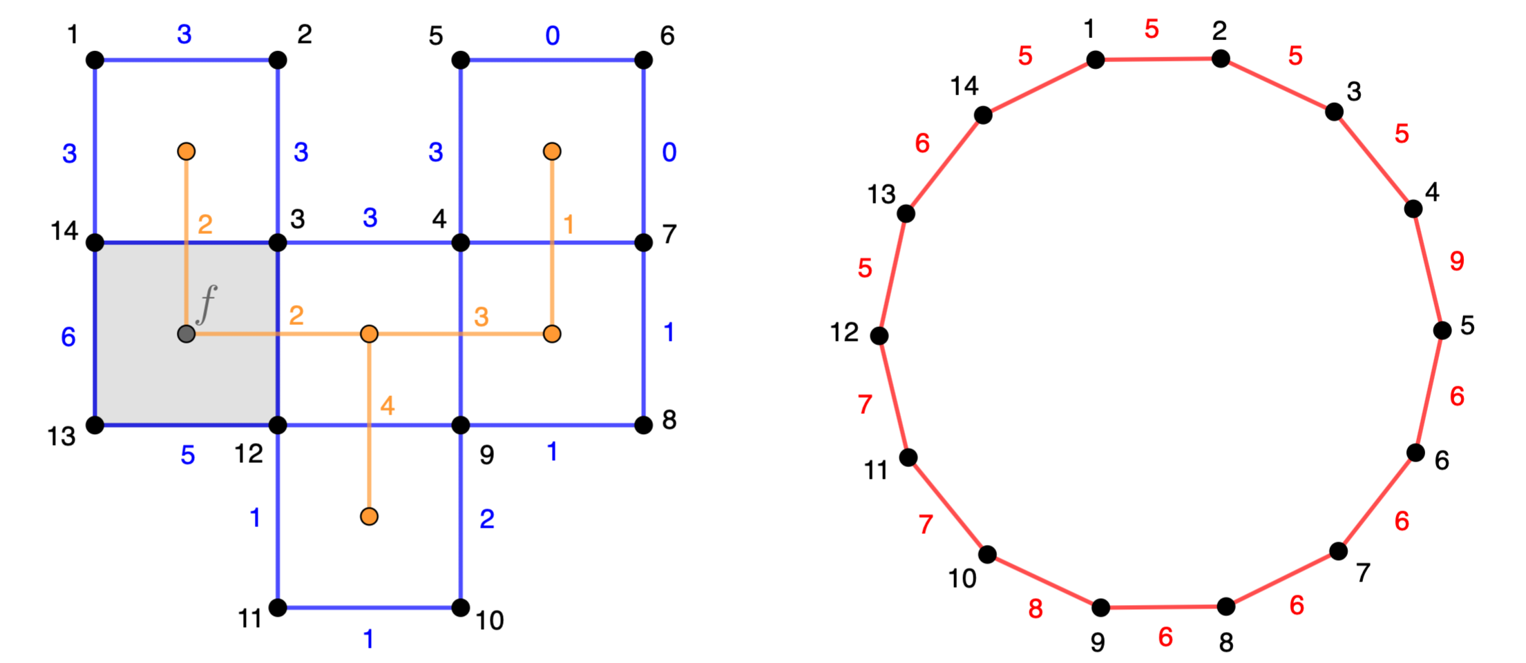
We would like to find an appropriate pinning of the demands in $D^{(k)}_{1}\cup D^{(k)}_{2}$ , and to this end, we create a ring-loading instance as follows. For $i\in[n]$ , let $f_{i}$ be the unique face in $\mathcal{F}-f_{\infty}$ containing the edge $\{i,i+1\}$ . We define the following ring-loading instance,

\mathcal{RL}([n],c_{\text{rl}},D^{(k)}_{1}\cup D^{(k)}_{2},d^{(k)})~\text{where}~c_{\text{rl}}(\{i,i+1\}):=x^{*}\big(G^{*}_{f,f_{i}}\big)+x^{*}(\{i,i+1\}).

(2)

See Figure 1 for an example. In Lemma 4.4 we show that the cut-condition is satisfied for this ring-loading instance, and hence we can use $\mathcal{A}_{RL}$ to obtain an $\alpha$ -feasible unsplitable flow $z=\sum_{h\in D^{(k)}_{1}\cup D^{(k)}_{2}}z_{h}$ .

For $h\in D^{(k)}_{1}\cup D^{(k)}_{2}$ , we overload notation and use $z_{h}$ to also denote the (unique) path along which $h$ is routed in $z$ . The manner in which we pin a demand $h$ depends on whether the path $z_{h}$ uses the vertices $i_{1},i_{\ell}$ or not. More precisely, we replace each demand $h\in D^{(k)}_{1}\cup D^{(k)}_{2}$ by a set of demands $D^{(k)}_{h}$ as described below.

Case 1: Suppose that $h\in D^{(k)}_{1}$ and $V(h)=\{s,t\}$ ; without loss of generality, we may assume that $s=i_{p}$ for some $1<p<\ell$ , and $t\in C^{(k)}\setminus V(f)$ . If $i_{1}\in z_{h}$ , then

D^{(k)}_{h}:=\{\{i_{j},i_{j+1}\}:1\leq j<p\}\cup\{\{i_{1},t\}\}.

(3)

Otherwise, if $i_{\ell}\in z_{h}$ , then

D^{(k)}_{h}:=\{\{i_{j},i_{j+1}\}:p\leq j<\ell\}\cup\{\{i_{\ell},t\}\}.

(4)

Case 2: Now suppose that $h\in D^{(k)}_{2}$ and $V(h)=\{s,t\}$ ; without loss of generality, we may assume that $s=i_{p}$ and $t=i_{q}$ for $1\leq p<q\leq\ell$ . If both $i_{1},i_{\ell}\in z_{h}$ , then:

D^{(k)}_{h}:=\{\{i_{j},i_{j+1}\}:1\leq j<p\}\cup\{\{i_{\ell},i_{1}\}\}\cup\{\{i_{j},i_{j+1}\}:q\leq j<\ell\}.

(5)

Otherwise; if either $i_{1}\notin z_{h}$ or $i_{\ell}\not\in z_{h}$ ,⁶⁶ 6 It may be the case that $|\{i_{1},i_{\ell}\}\cap V(z_{h})|=1$ , if either $p=1$ or $q=\ell$ . then:

D^{(k)}_{h}:=\{\{i_{j},i_{j+1}\}:p\leq j<q\}.

(6)

In item (c) of Lemma 4.3 we show that there is at most one bad demand edge in $\mathcal{W}_{g}^{(k)}$ . If $h\in\mathcal{W}_{g}^{(k)}$ for $h\in D^{(k)}_{1}\cup D^{(k)}_{2}$ , then we update $\mathcal{W}^{(k)}_{g}$ by removing $h$ and adding $D^{(k)}_{h}$ .

	$\displaystyle\mathcal{W}^{(k+1)}_{g}$	$\displaystyle\leftarrow(\mathcal{W}^{(k)}_{g}-h)\cup D^{(k)}_{h}$		$\displaystyle,\hskip 8.53581pt\text{if there exists $h\in\mathcal{W}^{(k)}_{g}$ with $h\in D^{(k)}_{1}\cup D^{(k)}_{2}$ };$
	$\displaystyle\mathcal{W}^{(k+1)}_{g}$	$\displaystyle\leftarrow\mathcal{W}^{(k)}_{g}$		$\displaystyle,\hskip 8.53581pt\text{otherwise.}$		(7)

We update $D^{(k)}$ as follows:

D^{(k+1)}\leftarrow\cup_{g\in D}\mathcal{W}^{(k+1)}_{g}

(8)

We also update $d^{(k+1)}$ accordingly. Let $\mathbbm{1}_{f}\in\{0,1\}^{E}$ be the characteristic vector of the edge set of $f$ . In Lemma 4.4, we show that the cut-condition is satisfied for the following instance:

\mathcal{I}\left(G,x^{*}+\alpha\cdot d_{{\max}}\cdot\mathbbm{1}_{f},D_{f},d^{(k+1)}\right)\hskip 8.53581pt\text{where}\hskip 8.53581ptD_{f}:=\cup_{h\in D^{(k)}_{1}\cup D^{(k)}_{2}}D^{(k)}_{h}.

(9)

We compute a feasible flow $y=\sum_{r\in D_{f}}y_{r}$ for this instance and set,

x^{(k+1)}\leftarrow x^{(k)}-x^{*}+y

(10)

As already mentioned, we increase the label of all the edges of $f$ by 1, and also increase their capacity by $\alpha\cdot d_{{\max}}$ . More precisely,

c^{(k+1)}\leftarrow c^{(k)}+\alpha\cdot d_{{\max}}\cdot\mathbbm{1}_{f}\hskip 8.53581pt\text{and}\hskip 8.53581pt\textsc{label}^{(k+1)}\leftarrow\textsc{label}^{\hskip-1.9919pt(k)}+\mathbbm{1}_{f}.

(11)

This completes the description of the algorithm. See Figure 2 for an example that illustrates how the demand edges could evolve on each iteration of the algorithm.

[Uncaptioned image] — Original instance with $D=\{{\color[rgb]{0,0.8,0}b},{\color[rgb]{1,0,1}g}\}$

4.2 Proof of Correctness

We first note a few key lemmas which are useful in proving Theorem 4.2. For any iteration $k\geq 1$ and $j\in\{0,1,2\}$ , let $E_{j}(k):=\{e\in E:\textsc{label}^{\hskip-1.9919pt(k)}(e)=j\}$ . Recall that $\textsc{label}^{\hskip-1.9919pt(k)}(e)$ denotes the label of $e$ at the start of iteration $k$ ; where we initially define $\textsc{label}^{\hskip-1.9919pt(1)}(e)=1$ if $e\in f_{\infty}$ , and $\textsc{label}^{\hskip-1.9919pt(1)}(e)=0$ if $e\in E\setminus E(f_{\infty})$ .

Lemma 4.3.

The following holds for each iteration $k\geq 1$ and $g\in D$ .

(a)

$E_{1}(k)$ is either the edge-set of a simple cycle $C^{(k)}$ in $G$ , or the empty set.
(b)

Consider the induced graph $G[C^{(k)}]$ on the vertex-set of $C^{(k)}$ . Then $E_{0}(k)$ are precisely the edges of $G[C^{(k)}]$ that do not lie on the cycle $C^{(k)}$ , and $E_{2}(k)$ are precisely the edges of $G$ that are not contained in $G[C^{(k)}]$ .
(c)

The demand edges in $\mathcal{W}_{g}^{(k)}$ form a walk between the end-points of $g$ . Furthermore, there is at most one bad demand edge $h\in\mathcal{W}_{g}^{(k)}$ . If such $h$ exists, then both of its end-points lie on the cycle $C^{(k)}$ .

Proof.

The proof is by induction on $k$ . The result clearly holds when $k=1$ . Suppose that $k\geq 2$ . By the induction hypothesis, the result holds for $k-1$ . We consider three cases.

Case 1: $E_{1}(k-1)=\emptyset$ .

By (b), it follows that $\textsc{label}^{\hskip-1.9919pt(k-1)}(e)=2$ for each $e\in E$ ; thus, the algorithm reaches its termination-condition at the start of iteration $(k-1)$ (in particular there is no iteration $k$ ).

Case 2: $E_{1}(k-1)\neq\emptyset$ and $G[C^{(k-1)}]=C^{(k-1)}$ .

Then the cycle $C^{(k-1)}$ is a face of $G$ . By (b), it follows that $\textsc{label}^{\hskip-1.9919pt(k-1)}(e)=2$ for all edges $e\in E\setminus E_{1}(k-1)$ . Thus $C^{(k-1)}$ is the (unbounded) face $f$ of $G$ processed in iteration $k-1$ . Since $\textsc{label}^{\hskip-1.9919pt(k)}=\textsc{label}^{\hskip-1.9919pt(k-1)}+\mathbbm{1}_{f}$ (see (11)), it follows that $\textsc{label}^{\hskip-1.9919pt(k)}(e)=2$ for each $e\in E$ . This proves (a) and (b). We now show (c). By the induction hypothesis, (i) there is at most one bad demand edge $h\in\mathcal{W}^{(k-1)}_{g}$ ; and (ii) $\mathcal{W}^{(k-1)}_{g}$ is the edge-set of a walk between the endpoints of $g$ . If such a bad demand edge $h$ does not exist, then $\mathcal{W}_{g}^{(k-1)}=\mathcal{W}_{g}^{(k)}$ (see (7)), and therefore (c) is trivially satisfied in this case. Suppose on the other hand that there is a bad demand edge $h\in\mathcal{W}^{(k-1)}_{g}$ . By (c), both end-points $s,t$ of $h$ lie on $C^{(k-1)}$ ; therefore $h\in D^{(k-1)}_{2}$ . At the end of iteration $k-1$ , edge $h$ is replaced by a sequence of demand edges $D^{(k-1)}_{h}$ which form a simple $s-t$ path along the edges of $C^{(k-1)}$ (see (5) and (6)). Thus, (i) $\mathcal{W}^{(k)}_{g}=(\mathcal{W}^{(k-1)}_{g}-h)\cup D^{(k-1)}_{h}$ only contains good demand edges; and (ii) $\mathcal{W}^{(k)}_{g}$ is the edge-set of a walk between the end-points of $g$ . This proves (c).

Case 3: $E_{1}(k-1)\neq\emptyset$ and $G[C^{(k-1)}]\neq C^{(k-1)}$ .

Then $C^{(k-1)}$ is not a bounded face⁷⁷ 7 Recall that all the faces of $G$ except $f_{\infty}$ are bounded of $G$ . Also, $G[C^{(k-1)}]$ is a (2-vertex connected) outerplanar graph and each bounded face of $G[C^{(k-1)}]$ is also a bounded face of $G$ . By Fact 2.4, the weak dual $G^{*}[C^{(k-1)}]$ of $G[C^{(k-1)}]$ is a tree. By (b), the edge-set $E_{0}(k-1)$ is precisely the edge-set of $G^{*}[C^{(k-1)}]$ ; therefore, the faces of $G$ that can be processed on iteration $k-1$ are precisely the faces representing the leaf nodes of $G^{*}[C^{(k-1)}]$ . Let $f=i_{1}i_{2}\ldots i_{\ell}i_{1}$ be the face that is processed on iteration $k-1$ . Then $\textsc{label}^{\hskip-1.9919pt(k-1)}(\{i_{j},i_{j+1}\})=1$ for each $1\leq j\leq\ell-1$ and $\textsc{label}^{\hskip-1.9919pt(k-1)}(\{i_{\ell},i_{1}\})=0$ . Let $\omega_{1}\omega_{2}\ldots\omega_{p}i_{1}i_{2}\ldots i_{\ell}\omega_{1}$ denote the node-sequence of the simple cycle $C^{(k-1)}$ , where $p\geq 1$ . Since $\textsc{label}^{\hskip-1.9919pt(k)}=\textsc{label}^{\hskip-1.9919pt(k-1)}+\mathbbm{1}_{f}$ , the edge-set $E_{1}(k)$ induces the simple cycle $C^{(k)}$ given by the node-sequence $\omega_{1}\omega_{2}\ldots\omega_{p}i_{1}i_{\ell}\omega_{1}$ . This proves (a). By the above, the only edge $e\in E$ such that $\textsc{label}^{\hskip-1.9919pt(k-1)}(e)=0$ and $\textsc{label}^{\hskip-1.9919pt(k)}(e)=1$ is $e=\{i_{\ell},i_{1}\}$ i.e., $E_{0}(k)=E_{0}(k-1)-\{i_{\ell},i_{1}\}$ . Therefore, $E_{0}(k)$ consists precisely of the edges $e$ of $G$ whose two endpoints lie on $C^{(k)}$ and $e\notin C^{(k)}$ . This proves (b). If $\mathcal{W}_{g}^{(k-1)}$ does not contain a bad demand edge, then $\mathcal{W}_{g}^{(k-1)}=\mathcal{W}_{g}^{(k)}$ , as observed before. Otherwise, $\mathcal{W}_{g}^{(k-1)}$ contains precisely one bad demand edge $h$ . By (c), both end-points $s,t$ of $h$ lie on $C^{(k-1)}$ . If neither $s$ nor $t$ are contained in $\{i_{2},i_{3},\ldots,i_{\ell}\}$ , then $h$ is not contained in $D^{(k)}_{1}\cup D^{(k)}_{2}$ during iteration $k-1$ ; in which case $\mathcal{W}^{(k)}_{g}=\mathcal{W}^{(k-1)}_{g}$ and $s,t\in G[C^{(k)}]$ . Otherwise, $h\in D^{(k)}_{1}\cup D^{(k)}_{2}$ . If $h\in D^{(k)}_{2}$ , then, by the same argument as in Case 2, (i) $\mathcal{W}^{(k)}_{g}=(\mathcal{W}^{(k-1)}_{g}-h)\cup D^{(k-1)}_{h}$ only contains good demand edges; and (ii) $\mathcal{W}^{(k)}_{g}$ is the edge-set of a walk between the end-points of $g$ . Thus assume that $h\in D^{(k)}_{1}$ , $s\in\{i_{2},i_{3},\ldots,i_{\ell-1}\}$ , and $t\in\{\omega_{1},\omega_{2},\ldots,\omega_{p}\}$ . If $\mathcal{W}^{(k)}_{g}$ contains a bad demand edge, then this edge is either $\{i_{1},t\}$ or $\{i_{\ell},t\}$ ; both of these possible demands edges have their two end-points in $C^{(k)}$ . Finally, since (a) $\mathcal{W}^{(k-1)}_{g}$ is the edge-set of a walk between the end-points of $g$ , and (b) $h$ gets replaced in $\mathcal{W}^{(k-1)}_{g}$ with the edge-set $D^{(k-1)}_{h}$ of an $s-t$ path (containing at most one bad demand edge), then $\mathcal{W}^{(k)}_{g}$ is the edge-set of a walk between the end-points of $G$ . This proves (c). ∎

Lemma 4.4.

Let $x$ be a feasible flow for $\mathcal{I}\left(G,c^{(k)},D^{(k)},d^{(k)}\right)$ , then the following hold:

(a)

The ring-loading instance $\mathcal{RL}\left([n],c_{\text{rl}},D^{(k)}_{1}\cup D^{(k)}_{2},d^{(k)}\right)$ defined at eq. 2 satisfies the cut-condition.
(b)

The instance $\mathcal{I}\left(G,x^{*}+\alpha\cdot d_{{\max}}\cdot\mathbbm{1}_{f},D_{f},d^{(k+1)}\right)$ defined at eq. 9 satisfies the cut-condition.

Proof.

Observe that at the start of iteration $k$ , $x^{*}$ is a feasible flow of $\mathcal{I}(G,x^{*},D^{(k)}_{1}\cup D^{(k)}_{2},d^{(k)})$ , and hence $\mathcal{I}(G,x^{*},D^{(k)}_{1}\cup D^{(k)}_{2},d^{(k)})$ satisfies the cut-condition, i.e.,

d^{(k)}\left(\delta_{D^{(k)}_{1}\cup D^{(k)}_{2}}\left(\,[i,j]\,\right)\right)\leq x^{*}\big(\delta_{G}\left(\,[i,j]\,\right)\big)\text{ for each }i,j\in[n].

(12)

Let $i,j\in[n]$ with $i\neq j+1$ , and $f_{1}$ and $f_{2}$ be the unique faces in $\mathcal{F}-f_{\infty}$ that contain $\{i-1,i\}$ and $\{j,j+1\}$ respectively. Then,

	$\displaystyle d^{(k)}\left(\delta_{D^{(k)}_{1}\cup D^{(k)}_{2}}\left(\,[i,j]\,\right)\right)$	$\displaystyle\leq x^{}\big(\delta_{G}\left(\,[i,j]\,\right)\big)\leq x^{}(G^{}_{f_{1},f})+x^{}(G^{}_{f,f_{2}})+x^{}(\{i-1,i\})+x^{*}(\{j,j+1\})$
		$\displaystyle=c_{\text{rl}}\big(\,\{i-1,i\}\,\big)+c_{\text{rl}}\big(\,\{j,j+1\}\,\big)=c_{\text{rl}}\big(\,\delta_{[n]}(\,[i,j]\,)\,\big).$

The first inequality follows from (12). The second inequality follows from Lemma 4.1. The first equality follows from the definition of $c_{\text{rl}}$ . It follows from Lemma 2.2 that $\mathcal{RL}([n],c_{\text{rl}},D^{(k)}_{1}\cup D^{(k)}_{2},d^{(k)})$ satisfies the cut-condition. This proves item (a). Hence, Algorithm $\mathcal{A}_{RL}$ computes a $\alpha$ -feasible unsplittable flow $z$ for $\mathcal{RL}\left([n],c_{\text{rl}},D^{(k)}_{1}\cup D^{(k)}_{2},d^{(k)}\right)$ . We now prove (b). By Lemma 2.2, it suffices to show that,

d^{(k+1)}\big(\delta_{D_{f}}\left(\,[i,j]\,\right)\big)\leq(x^{*}+\alpha\cdot d_{{\max}}\cdot\mathbbm{1}_{f})(\delta_{G}\left(\,[i,j]\,\right)\big)~\text{for}~i,j\in[n],i\neq j+1.

(13)

We consider three cases.

Case 1: $i,j\in\llparenthesis i_{\ell},i_{1}\rrparenthesis$ .

It suffices to show that,

d^{(k)}\left(\delta_{D^{(k)}_{1}\cup D^{(k)}_{2}}\left(\,[i,j]\,\right)\right)=d^{(k+1)}\big(\,\delta_{D_{f}}\left(\,[i,j]\,\right)\big),

since inequality (13) would then immediately follow from (12) in this case. Observe that: (i) all the edges in $D^{(k)}_{h}$ , for $h\in D^{(k)}_{2}$ , are only incident to nodes of $f$ ; and (ii) if $h\in D^{(k)}_{1}$ , then $t\in V(h)$ is the unique endpoint of $h$ contained in $\llparenthesis i_{\ell},i_{1}\rrparenthesis$ , and there is precisely one demand edge of $D^{(k)}_{h}$ with exactly one endpoint in $\llparenthesis i_{\ell},i_{1}\rrparenthesis$ , and this endpoint is $t$ . Then $\delta_{D^{(k)}_{2}}\left(\,[i,j]\,\right)=\emptyset$ and $\delta_{D^{(k)}_{h}}\left(\,[i,j]\,\right)=\emptyset$ for each $h\in(D^{(k)}_{1}\cup D^{(k)}_{2})\setminus\delta_{D^{(k)}_{1}}\left(\,[i,j]\,\right)$ . This implies that:

	$\displaystyle d^{(k)}\big(\delta_{D^{(k)}_{1}\cup D^{(k)}_{2}}([i,j])\big)$	$\displaystyle=\sum_{h\in\delta_{D^{(k)}_{1}}([i,j])}d^{(k)}(h);$
	$\displaystyle d^{(k)}\big(\delta_{D_{f}}([i,j])\big)$	$\displaystyle=\sum_{h\in\delta_{D^{(k)}_{1}}([i,j])}\sum_{r\in\delta_{D^{(k)}_{h}}([i,j])}d^{(k)}(r).$

Let $h\in\delta_{D^{(k)}_{1}}([i,j])$ . By observation (ii) above, $|\delta_{D^{(k)}_{h}}\left(\,[i,j]\,\right)|=1$ . Thus, since $d^{(k)}(r)=d^{(k)}(h)$ for each $r\in D^{(k)}_{h}$ , $d^{(k)}(h)=\sum_{r\in\delta_{D^{(k)}_{h}}([i,j])}d^{(k)}(r)$ . It follows that $d^{(k)}\big(\delta_{D^{(k)}_{1}\cup D^{(k)}_{2}}\left(\,[i,j]\,\right)\big)=d^{(k)}\big(\delta_{D_{f}}\left(\,[i,j]\,\right)\big)$ , as desired.

Case 2: $i,j\in\llparenthesis i_{q},i_{q+1}\rrparenthesis$ for some $1\leq q\leq\ell-1$ .

Then either $[i,j]\subseteq\llparenthesis i_{q},i_{q+1}\rrparenthesis$ or $[n]\setminus[i,j]\subseteq\llparenthesis i_{q},i_{q+1}\rrparenthesis$ . Since for each $h\in D^{(k)}_{1}\cup D^{(k)}_{2}$ , the demand edges in $D^{(k)}_{h}$ are incident only to nodes contained in either $f$ or $\llparenthesis i_{\ell},i_{1}\rrparenthesis$ , then either $[i,j]$ or $[n]\setminus[i,j]$ does not contain any node incident to edges of $D_{f}$ . Hence $\delta_{D_{f}}\left(\,[i,j]\,\right)=\emptyset$ , and inequality (13) follows trivially.

Case 3: $\{i,j\}\nsubseteq\llparenthesis i_{q},i_{q+1}\rrparenthesis$ for every $1\leq q\leq\ell$ , where $i_{\ell+1}:=i_{1}$ .

Then both $[i,j]$ and $[n]\setminus[i,j]$ contain at least one node from $f$ . Let $f_{1}$ and $f_{2}$ denote the unique faces in $\mathcal{F}-f_{\infty}$ that contain $\{i-1,i\}$ and $\{j,j+1\}$ , respectively. Since $z$ is an $\alpha$ -feasible unsplittable flow for $\mathcal{RL}\left([n],c_{\text{rl}},D^{(k)}_{1}\cup D^{(k)}_{2},d^{(k)}\right)$ , and by construction of $D_{f}$ , the ring-loading instance $\mathcal{RL}\left([n],c_{\text{rl}}+\alpha\cdot d_{{\max}},D_{f},d^{(k+1)}\right)$ is feasible. Therefore $\mathcal{RL}\left([n],c_{\text{rl}}+\alpha\cdot d_{{\max}},D_{f},d^{(k+1)}\right)$ satisfies the cut-condition. It follows that,

	$\displaystyle d^{(k+1)}\big(\delta_{D_{f}}\left(\,[i,j]\,\right)\big)$	$\displaystyle\leq\left(c_{\text{rl}}+\alpha\cdot d_{{\max}}\right)\big(\delta_{[n]}\left(\,[i,j]\,\right)\big)$
		$\displaystyle=c_{\text{rl}}\big(\,\{i-1,i\}\,\big)+c_{\text{rl}}\big(\,\{j,j+1\}\,\big)+2\cdot\alpha\cdot d_{{\max}}$
		$\displaystyle=x^{}\left(G^{}_{f,f_{1}}\right)+x^{}\big(\,\{i-1,i\}\,\big)+x^{}\left(G^{}_{f,f_{2}}\right)+x^{}\big(\,\{j,j+1\}\,\big)+2\cdot\alpha\cdot d_{{\max}}$
		$\displaystyle=x^{}\left(G^{}_{f_{1},f_{2}}\right)+x^{}\big(\,\{i-1,i\}\,\big)+x^{}\big(\,\{j,j+1\}\,\big)+2\cdot\alpha\cdot d_{{\max}}$
		$\displaystyle=\left(x^{*}+\alpha\cdot d_{{\max}}\cdot\mathbbm{1}_{f}\right)\big(\delta_{G}\left(\,[i,j]\,\right)\big).$

The second equality follows from the definition of $c_{\text{rl}}$ . The third equality follows from Lemma 4.1. The last equality follows from part (c) of Lemma 4.1, and the fact that there are precisely two edges of $f$ in $\delta_{G}\left(\,[i,j]\,\right)$ . This proves item (b). ∎

A consequence of Lemma 4.4 is that the instance $\mathcal{I}(G,c^{(k)},D^{(k)},d^{(k)})$ computed by the algorithm at the end of an iteration is feasible.

Lemma 4.5.

Let $x^{(k)}=\sum_{h\in D^{(k)}}x_{h}$ be a feasible flow for $\mathcal{I}\left(G,c^{(k)},D^{(k)},d^{(k)}\right)$ , then $x^{(k+1)}$ is a feasible flow for $\mathcal{I}\left(G,c^{(k+1)},D^{(k+1)},d^{(k+1)}\right)$ .

Proof.

Suppose that $f\in\mathcal{F}-f_{\infty}$ is the face being considered in iteration $k$ . Since $x^{(k)}$ is a feasible flow for instance $\mathcal{I}\left(G,c^{(k)},D^{(k)},d^{(k)}\right)$ , it follows that $x^{(k)}-x^{*}$ is a feasible flow for instance $\mathcal{I}\left(G,c^{(k)}-x^{*},D^{(k)}\setminus\left(D^{(k)}_{1}\cup D^{(k)}_{2}\right),d^{(k)}\right)$ . By Lemma 4.4, $\mathcal{I}\left(G,x^{*}+\alpha\cdot d_{{\max}}\cdot\mathbbm{1}_{f},D_{f},d^{(k+1)}\right)$ (defined at eq. 9) satisfies the cut-condition. Therefore, by Theorem 2.1 a feasible flow $y$ of $\mathcal{I}\left(G,x^{*}+\alpha\cdot d_{{\max}}\cdot\mathbbm{1}_{f},D_{f},d^{(k+1)}\right)$ can be computed (in polynomial time). It then follows that $x^{(k)}-x^{*}+y$ is a feasible flow for $\mathcal{I}\left(G,c^{(k)}+\alpha\cdot d_{{\max}}\cdot\mathbbm{1}_{f},\left(D^{(k)}\setminus\left(D^{(k)}_{1}\cup D^{(k)}_{2}\right)\right)\cup D_{f},d^{(k+1)}\right)$ The proof of the lemma follows from the fact that $x^{(k+1)}=x^{(k)}-x^{*}+y$ , and

\mathcal{I}(G,c^{(k+1)},D^{(k+1)},d^{(k+1)})=\mathcal{I}\left(G,c^{(k)}+\alpha\cdot d_{{\max}}\cdot\mathbbm{1}_{f},\left(D^{(k)}\setminus\left(D^{(k)}_{1}\cup D^{(k)}_{2}\right)\right)\cup D_{f},d^{(k+1)}\right).

∎

We are now ready to give a proof of Theorem 4.2, which we restate. See 4.2

Proof.

By Lemma 4.5, the cut-condition is satisfied for each $\mathcal{I}(G,c^{(k)},D^{(k)},d^{(k)})$ , and hence the cut-condition is also satisfied for the final output $\mathcal{I}(G,c^{\prime},D^{\prime},d^{\prime})$ . Note that the capacity of an edge $e$ is increased by $\alpha\cdot d_{\max}$ only when its label is also increased by 1. Initially, the label of all the edges on the unbounded face $f_{\infty}$ is 1 while the label of the remaining edges is 0. At the end of the algorithm, the label of every edge is 2. This implies that the capacity of edges on $f_{\infty}$ increases by $\alpha\cdot d_{{\max}}$ and the capacity of the remaining edges increases by $2\cdot\alpha\cdot d_{{\max}}$ . By item (c) of Lemma 4.3, it follows that the edges in $W_{g}$ form a walk between the end points of $g$ . Furthermore, if there are bad edges in $W_{g}$ , then both its end-points are incident on the cycle formed by label 1 edges. At the end of the algorithm, there are no label 1 edges and hence there are no bad edges in $W_{g}$ . Whenever we insert a new demand edge in $\mathcal{W}_{g}^{(k)}$ , we set its value to $d(g)$ . Hence all the demand edges in $W_{g}$ have value $d(g)$ , and this completes the proof. ∎

4.3 Handling Parallel Edges in $G$

Suppose that $G=(V,E)$ has parallel edges. We describe how to proceed in this case. For every $u,v\in V$ , let $E(u,v)$ denote the edges incident to both $u$ and $v$ . We can create a new graph $G_{0}=(V,E_{0})$ by replacing each $E(u,v)\neq\emptyset$ with an edge $uv$ of capacity $c_{0}(uv)=\sum_{e\in E(u,v)}c(e)$ . Then $\mathcal{I}(G,c,D,d)$ is feasible if and only if $\mathcal{I}(G_{0},c_{0},D,d)$ is feasible. We can apply the algorithm in this section to $\mathcal{I}(G_{0},c_{0},D,d)$ in order to obtain an instance $\mathcal{I}(G_{0},c_{0}^{\prime},D^{\prime},d^{\prime})$ satisfying the properties in Theorem 4.2. For each $uv\in E_{0}$ , if $c_{0}^{\prime}(uv)=c_{0}(uv)+\delta$ , then pick an edge $e\in E(u,v)$ and define $c^{\prime}(e)=c(e)+\delta$ and $c^{\prime}(e^{\prime})=c(e^{\prime})$ for all $e^{\prime}\in E(u,v)-e$ . Then , the instance $\mathcal{I}(G,c^{\prime},D^{\prime},d^{\prime})$ satisfies the properties of Theorem 4.2 with respect to $\mathcal{I}(G,c,D,d)$ .

5 Proof of Theorem 3.2

In this section, we give a proof of Theorem 3.2, which we restate for convenience. See 3.2 As discussed in Section 2, we may assume without loss of generality that $G=(V,E)$ is 2-vertex connected. For any pair $u\neq v\in V$ of nodes, we use $E(u,v):=\{e\in E:V(e)=\{u,v\}\}$ and $D(u,v):=\{g\in D:V(g)=\{u,v\}\}$ to denote the set of edges of $E$ and $D$ , respectively, incident to both $u$ and $v$ . We say that an unbounded face $f=i_{1}i_{2}\ldots i_{\ell}i_{1}$ of $G$ is an ear incident to $\{i_{\ell},i_{1}\}$ , if $\ell\geq 3$ and if for every $j\in[\ell-1]$ , there exists an edge $e\in E(i_{\ell},i_{j+1})$ incident to the unbounded face of $G$ . ⁸⁸ 8 Observe that if we create a graph $G_{0}$ by replacing each $E(u,v)\neq\emptyset$ in $G$ with a single edge $uv$ , then an ear of $G$ corresponds to a leaf of the weak dual of $G_{0}$ .

We first give a brief description of the algorithm. Our algorithm works in iterations; one per each unbounded face of $G$ incident to at least $3$ vertices. At the start of iteration $k$ we consider a feasible instance $\mathcal{I}(G^{(k)},c^{(k)},D^{(k)},d^{(k)})$ where all demand edges are good and where $G^{(k)}$ is 2-vertex connected . Initially, $\mathcal{I}(G^{(1)},c^{(1)},D^{(1)},d^{(1)})=\mathcal{I}(G,c,D,d)$ . We consider an ear $f$ of $G^{(k)}$ incident to some $\{i_{\ell},i_{1}\}$ . For each $j\in[\ell-1]$ , each demand $g\in D^{(k)}(i_{j},i_{j+1})$ is either routed along a single edge of $E^{(k)}(i_{j},i_{j+1})$ , or $g$ is replaced with a demand of value $d^{(k)}(g)$ incident to $i_{1},i_{\ell}$ after routing a flow of value $d^{(k)}(g)$ both from $i_{j}$ to $i_{1}$ , and from $i_{j+1}$ to $i_{\ell}$ , across two paths with node sequence $i_{j}\ldots i_{1}$ and $i_{j+1}\ldots i_{\ell}$ , respectively. We do this so that the capacity of any edge is not exceeded by more than $d_{{\max}}$ . After this procedure, there are no demands incident to $i_{2},\ldots,i_{\ell-1}$ . If there is one $j\in[\ell-1]$ , such that all edges $e$ in $E^{(k)}(i_{j},i_{j+1})$ have exceeded their original capacity $c^{(k)}(e)$ , we remove $\{i_{2},\ldots,i_{\ell-1}\}$ from $G^{(k)}$ ; otherwise, we replace $\{i_{2},\ldots,i_{\ell-1}\}$ and their incident edges with a single edge $e_{0}=\{i_{1},i_{\ell}\}$ with a suitable capacity. We then continue to iteration $k+1$ , and in there we consider any ear from the graph of the resulting instance. After the last iteration, the resulting (feasible) instance has a supply graph with only two vertices, which is straightforward to solve, for instance, by using Claim 5.1 below.

Iteration $k$ proceeds differently, depending on which of the following two cases hold:

	Case 1:	$\displaystyle\sum_{g\in D^{(k)}(i_{j},i_{j+1})}d^{(k)}(g)\leq d_{{\max}}+\sum_{e\in E^{(k)}(i_{j},i_{j+1})}c^{(k)}(e)\text{ for each }j\in[\ell-1].$
	Case 2:	$\displaystyle\sum_{g\in D^{(k)}(i_{j},i_{j+1})}d^{(k)}(g)>d_{{\max}}+\sum_{e\in E^{(k)}(i_{j},i_{j+1})}c^{(k)}(e)\text{ for precisely one }j\in[\ell-1].$		(14)

Observe that if $\mathcal{I}(G^{(k)},c^{(k)},D^{(k)},d^{(k)})$ satisfies the cut-condition, then it cannot be the case that there are $1\leq j<j^{\prime}\leq\ell-1$ with $\sum_{g\in D^{(k)}(i_{j},i_{j+1})}d^{(k)}(g)>d_{{\max}}+\sum_{e\in E^{(k)}(i_{j},i_{j+1})}c^{(k)}(e)$ and $\sum_{g\in D^{(k)}(i_{j^{\prime}},i_{{j^{\prime}}+1})}d^{(k)}(g)>d_{{\max}}+\sum_{e\in E^{(k)}(i_{j^{\prime}},i_{j^{\prime}+1})}c^{(k)}(e)$ . This holds because,

	$\displaystyle\sum_{e\in E(i_{j},i_{j+1})}c^{(k)}(e)+\sum_{e\in E(i_{j^{\prime}},i_{j^{\prime}+1})}c^{(k)}(e)$	$\displaystyle=c^{(k)}(\{i_{j+1},i_{j+2},\ldots,i_{j^{\prime}}\})\geq d^{(k)}(\{i_{j+1},i_{j+2},\ldots,i_{j^{\prime}}\})$
		$\displaystyle=\sum_{g\in D^{(k)}(i_{j},i_{j+1})}d^{(k)}(g)+\sum_{g\in D^{(k)}(i_{j^{\prime}},i_{j^{\prime}+1})}d^{(k)}(g),$

where the equalities follow from the fact that $f=i_{1}i_{2}\ldots i_{\ell}i_{1}$ is an ear of $G^{(k)}$ .

In order to prove Theorem 3.2, we make repeated use of the following straightforward claims.

Claim 5.1.

Consider an instance $\mathcal{I}(G,c,D,d)$ . Let $v_{1},v_{2}\ldots,v_{r}\in V$ be a set of distinct vertices, and let $D^{*}\subseteq D$ be a set of demand edges such that $V(g)=\{v_{1},v_{r}\}$ for all $g\in D^{*}$ . If

\sum_{g\in D^{*}}d(g)\leq d_{{\max}}+\sum_{e\in E(v_{j},v_{j+1})}c(e),\;\forall j\in[r-1],

then one can efficiently compute a set of paths $\{p_{g}\}_{g\in D^{*}}$ in $G$ such that the node sequence of each $p_{g}$ is precisely $v_{1}v_{2}\ldots v_{r}$ , and such that

\sum_{g\in D^{*}:e\in p_{g}}d(g)\leq c(e)+d_{{\max}},\;\forall e\in\{E(v_{j},v_{j+1})\}_{j\in[r-1]}.

Proof.

Let $j\in[r-1]$ . Suppose that $E(i_{j},i_{j+1})=\{e_{1},\ldots,e_{a}\}$ and $D(i_{j},i_{j+1})=\{g_{1},\ldots,g_{b}\}$ . It suffices to prove that we can compute an assignment $\sigma_{j}:D^{*}\rightarrow E(i_{j},i_{j+1})$ , such that $\sum_{g\in D^{*}:\sigma_{j}(g)=e}d(g)\leq c(e)+d_{{\max}}$ for each $e\in E(v_{j},v_{j+1})$ . The proof of the theorem would then follow by taking $p_{g}=\{\sigma_{j}(g)\}_{j\in[\ell-1]}$ . We prove the above by induction on $|E(i_{j},i_{j+1})|$ . Clearly, the above holds if $|E(i_{j},i_{j+1})|=1$ . Thus, suppose that $|E(i_{j},i_{j+1})|>1$ . Take any edge $e^{\prime}\in E(v_{j},v_{j+1})$ , and let $Q\subseteq D^{*}$ be a maximal inclusion-wise subset of demands with $\sum_{g\in Q}d(g)\leq c(e^{\prime})+d_{{\max}}$ . Let $\sigma_{j}(g)=e^{\prime}$ for all $g\in Q$ . If $Q=D^{*}$ , we are done. If $Q\neq D^{*}$ , then $c(e^{\prime})<\sum_{g\in Q}d(g)$ . Therefore, $\sum_{g\in D^{*}\setminus Q}d(g)\leq d_{{\max}}+\sum_{e\in E(v_{j},v_{j+1})-e^{\prime}}c(e)$ . By the induction hypothesis, we can assign each $g\in D^{*}\setminus Q$ to some edge in $E(v_{j},v_{j+1})-e^{\prime}$ , so that $\sum_{g\in D^{*}\setminus Q:\sigma_{j}(g)=e}d(g)\leq c(e)+d_{{\max}}$ for each $e\in E(v_{j},v_{j+1})-e^{\prime}$ . ∎

Claim 5.2.

Suppose that an instance $\mathcal{I}(G,c,D,d)$ satisfies the cut-condition. Let $g\in D$ be a good demand with $V(g)=\{u,v\}$ . Suppose that one routes $g$ through some $e^{\prime}\in E(u,v)$ , by possibly exceeding the capacity of $e^{\prime}$ . Then the residual instance $\mathcal{I}(G,c^{\prime},D-g,d)$ satisfies the cut-condition, where $c^{\prime}(e^{\prime})=\max\{0,c(e^{\prime})-d(g)\}$ and $c^{\prime}(e)=c(e)$ for each $e\in E-e^{\prime}$ .

Proof.

Let $S\subseteq V$ . Clearly, the cut-condition holds if $u,v\in S$ or $u,v\in V\setminus S$ . If suffices to consider the case in which, without loss of generality, $u\in S$ and $v\notin S$ . Observe that,

c^{\prime}(\delta_{G}(S))=c(\delta_{G}(S))-c(e^{\prime})+c^{\prime}(e^{\prime})\geq d(\delta_{D}(S))-c(e^{\prime})+c^{\prime}(e^{\prime})\geq d(\delta_{D}(S))-d(g).

∎

For each case in (14), we show how to construct the feasible instance $\mathcal{I}(G^{(k+1},c^{(k+1)},D^{(k+1)},d^{(k+1)})$ , and show how to convert a 1-feasible unsplittable flow in $\mathcal{I}(G^{(k+1)},c^{(k+1)},D^{(k+1)},d^{(k+1)})$ into a 1-feasible unsplittable flow in $\mathcal{I}(G^{(k)},c^{(k)},D^{(k)},d^{(k)})$ .

5.1 Description of an Iteration in Case 1

Suppose that $\sum_{g\in D^{(k)}(i_{j},i_{j+1})}d^{(k)}(g)\leq d_{{\max}}+\sum_{e\in E^{(k)}(i_{1},i_{j+1})}c^{(k)}(e)$ for all $j\in[\ell-1]$ . By Claim 5.1, we can assign each $g\in D^{(k)}(i_{j},i_{j+1})$ to an edge $e_{g}\in E^{(k)}(i_{j},i_{j+1})$ , so that $d_{e}\leq c(e)+d_{{\max}}$ for each $e\in E^{(k)}(i_{j},i_{j+1})$ , where $d_{e}:=\sum_{g\in D^{(k)}(i_{j},i_{j+1}):e_{g}=e}d^{(k)}(g)$ . After this operation, define $E_{j}=\{e\in E^{(k)}(i_{j},i_{j+1}):d_{e}\leq c^{(k)}(e)\}$ as the set of edges whose capacity was not exceeded during the above procedure. Create a new edge $e_{0}$ incident to $i_{1}$ and $i_{\ell}$ , and define

	$\displaystyle V^{(k+1)}$	$\displaystyle:=V^{(k)}\setminus\{i_{2},\ldots,i_{\ell-1}\},$
	$\displaystyle E^{(k+1)}$	$\displaystyle:=\left(E^{(k)}\setminus\cup_{j\in[\ell-1]}E^{(k)}(i_{j},i_{j+1})\right)+e_{0},$
	$\displaystyle c^{(k+1)}(e)$	$\displaystyle:=\begin{cases}c^{(k)}(e),&\>\text{if }~e\in E^{(k)}\setminus\cup_{j\in[\ell-1]}E^{(k)}(i_{j},i_{j+1})\\ \min_{j\in[\ell-1]}\sum_{e\in E_{j}}(c^{(k)}(e)-d_{e}),&\>\text{if }~e=e_{0},\end{cases}$
	$\displaystyle D^{(k+1)}$	$\displaystyle:=D^{(k)}\setminus\cup_{j\in[\ell-1]}D^{(k)}(i_{j},i_{j+1}),$
	$\displaystyle d^{(k+1)}(g)$	$\displaystyle:=d^{(k)}(g).$

Claim 5.3.

$\mathcal{I}(G^{(k+1)},c^{(k+1)},D^{(k+1)},d^{(k+1)})$ is feasible.

Proof.

By Claim 5.2, the residual instance $\mathcal{I}_{res}$ obtained from $\mathcal{I}(G^{(k)},c^{(k)},D^{(k)},d^{(k)})$ after routing the demands in $\{D^{(k)}(i_{j},i_{j+1})\}_{j\in[\ell-1]}$ , replacing $\{E^{(k)}(i_{j},i_{j+1})\}_{j\in[\ell-1]}$ with $\{E_{j}\}_{j\in[\ell-1]}$ , and decreasing $c^{(k)}(e)$ by $d_{e}$ , is feasible. The claim follows from the Max Flow-Min Cut Theorem, by observing that $\mathcal{I}_{res}$ does not have demands incident to any node in $\{i_{2},\ldots,i_{\ell-1}\}$ , and that $\mathcal{I}(G^{(k+1)},c^{(k+1)},D^{(k+1)},d^{(k+1)})$ is obtained from $\mathcal{I}_{res}$ by replacing $\{E_{j}\}_{j\in[\ell-1]}$ with $e_{0}$ . ∎

Claim 5.4.

A 1-feasible unsplittable flow $y$ in $\mathcal{I}(G^{(k+1)},c^{(k+1)},D^{(k+1)},d^{(k+1)})$ can be efficiently converted into a 1-feasible unsplittable flow $z$ in $\mathcal{I}(G^{k},c^{(k)},D^{(k)},d^{(k)})$ .

Proof.

Let $y(g)$ be the edge set of the path on which $y$ routes $g\in D^{(k+1)}$ . For each $g\in\cup_{j\in[\ell-1]}D^{(k)}(i_{j},i_{j+1})$ , let $z(g)=\{e_{g}\}$ . For the remaining demands of $D^{(k)}$ i.e., the demands in $D^{(k+1)}$ , we consider two cases. For each $g\in D^{(k+1)}$ with $e_{0}\notin y(g)$ , let $z(g)=y(g)$ . Let $D_{0}\subseteq D^{(k+1)}$ be the set of demands $g$ with $e_{0}\in y(g)$ . Let $y(e_{0})$ be the flow that traverses $e_{0}$ . Then,

y(e_{0})\leq d_{{\max}}+c^{(k+1)}(e_{0})=d_{{\max}}+\min_{j\in[\ell-1]}\sum_{e\in E_{j}}(c^{(k)}(e)-d_{e}).

It follows from Claim 5.1 that we can compute a set of paths $\{p_{g}\}_{g\in D_{0}}$ in $\cup_{j\in[\ell-1]}E_{j}$ , each of which has the node sequence $i_{1}i_{2}\ldots i_{\ell}$ , such that for each $e\in\cup_{j\in[\ell-1]}E_{j}$ ,

\sum_{g\in D_{0}:e\in p_{g}}d^{(k)}(g)\leq c^{(k)}(e)-d_{e}+d_{{\max}}.

For each $g\in D_{0}$ , we set $z(g)=(y(g)-e_{0})\cup p_{g}$ . Therefore, for each $e\in\cup_{j\in[\ell-1]}E_{j}$ ,

	$\displaystyle z(e)$	$\displaystyle=\sum_{g\in D^{k}(i_{j},i_{j+1}):z(g)=e}d^{(k)}(g)+\sum_{g\in D_{0}:e\in p_{g}}d^{(k)}(g)$
		$\displaystyle\leq d_{e}+c^{(k)}(e)-d_{e}+d_{{\max}}\leq c^{(k)}(e)+d_{{\max}}.$

Finally, note that $z(e)=d_{e}\leq c^{(k)}(e)+d_{{\max}}$ for each $e\in\cup_{j\in[\ell-1]}\left(E^{(k)}(i_{j},i_{j+1})\setminus E_{j}\right)$ , and that $z(e)=y(e)\leq c^{(k+1)}(e)+d_{{\max}}=c^{(k)}(e)+d_{{\max}}$ for each $e\in E^{(k)}\setminus\cup_{j\in[\ell-1]}E^{(k)}(i_{j},i_{j+1})$ . ∎

5.2 Description of an Iteration in Case 2

Let $j^{\prime}$ be the unique index in $[\ell-1]$ for which $\sum_{g\in D^{(k)}(i_{j^{\prime}},i_{j^{\prime}+1})}d^{(k)}(g)>d_{{\max}}+\sum_{e\in E^{(k)}(i_{j^{\prime}},i_{j^{\prime}+1})}c^{(k)}(e)$ . As in Case 1, for each $j^{\prime}\neq j\in[\ell-1]$ , we can assign each $g\in D^{(k)}(i_{j},i_{j+1})$ to an edge $e_{g}\in E^{(k)}(i_{j},i_{j+1})$ , so that $d_{e}\leq c(e)+d_{{\max}}$ for each $e\in E^{(k)}(i_{j},i_{j+1})$ , where $d_{e}=\sum_{g\in D^{(k)}(i_{j},i_{j+1}):e_{g}=e}d^{(k)}(g)$ . Take an inclusion-wise maximal subset $D^{*}_{j^{\prime}}\subseteq D^{(k)}(i_{j^{\prime}},i_{j^{\prime}+1})$ , such that each $g\in D^{*}$ can be mapped to an edge $e_{g}\in E^{(k)}(i_{j^{\prime}},i_{j^{\prime}+1})$ , so that $\sum_{g\in D^{*}_{j^{\prime}}:e_{g}=e}d^{(k)}(g)\leq c(e)+d_{{\max}}$ for each $e\in E^{(k)}(i_{j^{\prime}},i_{j^{\prime}+1})$ . If $D^{*}_{j^{\prime}}=D^{(k)}(i_{j^{\prime}},i_{j^{\prime}+1})$ , we can proceed in the exact same way as in Case 1 and define $\mathcal{I}(G^{(k+1)},c^{(k+1)},D^{(k+1)},d^{(k+1)})$ as there. Thus, assume that $D^{*}_{j^{\prime}}\neq D^{(k)}(i_{j^{\prime}},i_{j^{\prime}+1})$ . Let $D^{\#}_{j^{\prime}}=D^{(k)}(i_{j^{\prime}},i_{j^{\prime}+1})\setminus D^{*}_{j^{\prime}}$ . For each $g\in D^{\#}_{j^{\prime}}$ , we create a new demand edge $g^{\#}$ incident to $i_{1},i_{\ell}$ . Define,

	$\displaystyle V^{(k+1)}$	$\displaystyle:=V^{(k)}\setminus\{i_{2},\ldots,i_{\ell-1}\},$
	$\displaystyle E^{(k+1)}$	$\displaystyle:=E^{(k)}\setminus\{E(i_{j},i_{j+1})\}_{j\in[\ell-1]},$
	$\displaystyle c^{(k+1)}(e)$	$\displaystyle:=c^{(k)}(e),$
	$\displaystyle D^{(k+1)}$	$\displaystyle:=\left(D^{(k)}\setminus\cup_{j\in[\ell-1]}D^{(k)}(i_{j},i_{j+1})\right)\cup\{g^{\#}\}_{g\in D_{j^{\prime}}^{\#}}.$
	$\displaystyle d^{(k+1)}(g)$	$\displaystyle:=\begin{cases}d^{(k)}(g),&\>\text{if }~g\in D^{(k)}\setminus\cup_{j\in[\ell-1]}D^{(k)}(i_{j},i_{j+1})\\ d^{(k)}(h),&\>\text{if }~g=h^{\#}.\end{cases}$

Claim 5.5.

$\mathcal{I}(G^{(k+1)},c^{(k+1)},D^{(k+1)},d^{(k+1)})$ is feasible.

Proof.

As in Case 1, define $E_{j}=\{e\in E^{(k)}(i_{j},i_{j+1}):d_{e}\leq c^{(k)}(e)\}$ for each $j\in[\ell-1]$ . By Claim 5.2, the residual instance $\mathcal{I}_{\text{res}}=\mathcal{I}(G^{\prime}=(V^{(k)},E^{\prime}),c^{\prime},D^{\prime},d^{(k)})$ obtained from $\mathcal{I}(G^{(k)},c^{(k)},D^{(k)},d^{(k)})$ after routing the demands in $\left(\cup_{j\in[\ell-1]}D^{(k)}(i_{j},i_{j+1})\right)\setminus D^{\#}_{j^{\prime}}$ and deleting $\cup_{j\in[\ell-1]}(E^{(k)}(i_{j},i_{j+1})\setminus E_{j})$ , is feasible. Since $E_{j^{\prime}}=\emptyset$ , both $i_{1}$ and $i_{\ell}$ are cut-vertices of $G^{\prime}$ . Therefore, the cut-condition is maintained if we replace (pin) each $g\in D^{\#}_{j^{\prime}}$ in $\mathcal{I}_{res}$ with the three demand edges $g_{a}=\{i_{j^{\prime}},i_{1}\},\,g^{\#}=\{i_{1},i_{\ell}\},\,g_{b}=\{i_{\ell},i_{j^{\prime}+1}\}$ of the same demand value as $g$ . We can then split $\mathcal{I}_{res}$ into the three feasible instances $\mathcal{I}(G^{(k+1)},c^{(k+1)},D^{(k+1)},d^{(k+1)})$ , $\mathcal{I}_{a}=\mathcal{I}(G_{a}=(V_{a},E_{a}),c^{\prime},\{g_{a}:g\in D^{\#}_{j^{\prime}}\},d^{\prime})$ , and $\mathcal{I}_{b}=\mathcal{I}(G_{b}=(V_{b},E_{b}),c^{\prime},\{g_{b}:g\in D^{\#}_{j^{\prime}}\},d^{\prime})$ , where $V_{a}=\{i_{1},\ldots,i_{j^{\prime}}\}$ , $V_{b}=\{i_{j^{\prime}+1},\ldots,i_{\ell}\}$ , $E_{a}=\cup_{j\in[j^{\prime}-1]}E_{j}$ , $E_{b}=\cup_{j\in\{j^{\prime}+1,\ldots,\ell-1\}}E_{j}$ , and $d^{\prime}(g_{a})=d^{\prime}(g_{b})=d^{(k)}(g)$ . ∎

Claim 5.6.

Proof.

Let $z(g)=y(g)$ for each $g\in D^{(k)}\setminus\cup_{j\in[\ell-1]}D^{(k)}(i_{j},i_{j+1})$ , and let $z(g)=e_{g}$ for each $g\in\left(\cup_{j\in[\ell-1]}D^{(k)}(i_{j},i_{j+1})\right)\setminus D^{\#}_{j^{\prime}}$ . Let $\mathcal{I}_{a}$ and $\mathcal{I}_{b}$ be as in the proof of Claim 5.5. By Claim 5.1, we can compute two $1$ -feasible unsplittable flows $z_{a}$ , $z_{b}$ for $\mathcal{I}_{a}$ and $\mathcal{I}_{b}$ , respectively. For each $g\in D^{\#}_{j^{\prime}}$ , we set $z(g)=z_{a}(g_{a})\cup y(g^{\#})\cup z_{b}(g_{b})$ . Observe that $z(e)=d_{e}\leq c^{(k)}(e)+d_{{\max}}$ for each $e\in\cup_{j\in[\ell-1]}\left(E^{(k)}(i_{j},i_{j+1})\setminus E_{j}\right)$ , and $z(e)=y(e)\leq c^{(k+1)}(e)+d_{{\max}}=c^{(k)}(e)+d_{{\max}}$ for each $e\in E^{(k)}\setminus\cup_{j\in[\ell-1]}E^{(k)}(i_{j},i_{j+1})$ . Finally, let $c\in\{a,b\}$ and $e\in E_{c}$ . Then,

z(e)=d_{e}+z_{c}(e)\leq d_{e}+c^{\prime}(e)+d_{{\max}}=d_{e}+c^{(k)}(e)-d_{e}+d_{{\max}}=c^{(k)}(e)+d_{{\max}}.

∎

5.3 Proof of Theorem 3.2

Let $\mathcal{I}(G,c,D,d)$ be a feasible instance and let $F$ be the number of unbounded faces of $G$ with at least 3 vertices. For each iteration $k\in[F+1]$ , we compute the feasible instances $\mathcal{I}(G^{(k)},c^{(k)},D^{(k)},d^{(k)})$ as described above. Observe that each instance only contains good demands, and that each $G^{(k)}$ is a 2-vertex connected planar graph. In the end, $\mathcal{I}(G^{(F+1)},c^{(F+1)},D^{(F+1)},d^{(F+1)})$ has no unbounded faces with at least 3 vertices. Thus, $G^{(F+1)}$ contains only 2 vertices. By Claim 5.1, we can compute a 1-feasible unsplittable flow in $\mathcal{I}(G^{(F+1)},c^{(F+1)},D^{(F+1)},d^{(F+1)})$ . By Claims 5.4 and 5.6, we can backtrack starting from $k=F$ in order to compute a 1-feasible unsplittable flow in $\mathcal{I}(G^{(1)},c^{(1)},D^{(1)},d^{(1)})=\mathcal{I}(G,c,D,d)$ . This concludes the proof.

6 Conclusion

We proved that if $G$ is an outerplanar graph and the cut-condition is satisfied, then there exists a $\mathcal{O}(1)$ -feasible unsplittable flow. It is an interesting open problem to generalize this result to other settings where the cut-condition is also sufficient for a feasible routing of all the demands, for example when all the source-sink pairs are incident on the unbounded face of a planar graph. It would also be interesting to see if a similar result holds for a more general class of graphs, where the cut-condition is not sufficient for a feasible routing, such as series-parallel graphs.

References

[CS94] Steve Cosares and Iraj Saniee “An optimization problem related to balancing loads on SONET rings” In Telecommunication Systems 3 Springer, 1994, pp. 165–181
[Däu19] Karl Däubel “An improved upper bound for the ring loading problem” In Proceedings of the 17th International Workshop on Approximation and Online Algorithms, WAOA2019, 2019, pp. 89–105
[DGG99] Yefim Dinitz, Naveen Garg and Michel. Goemans “On the single-source unsplittable flow problem” In Combinatorica 19.1 Springer, 1999, pp. 17–41
[FF56] Lester Ford and Delbert. Fulkerson “Maximal flow through a network” In Canadian journal of Mathematics 8 Cambridge University Press, 1956, pp. 399–404
[GR01] Chris Godsil and Gordon. Royle “Algebraic graph theory” New York, USA: Springer, 2001
[Kle96] Jon. Kleinberg “Single-source unsplittable flow” In Proceedings of 37th Conference on Foundations of Computer Science, 1996, pp. 68–77 IEEE
[OS81] Haruko Okamura and Paul. Seymour “Multicommodity flows in planar graphs” In Journal of Combinatorial Theory, Series B 31.1 Elsevier, 1981, pp. 75–81
[Sch03] Alexander Schrijver “Combinatorial optimization: polyhedra and efficiency” Springer Science & Business Media, 2003
[Sey81] Paul. Seymour “On odd cuts and plane multicommodity flows” In Proceedings of the London Mathematical Society 3.1 Wiley Online Library, 1981, pp. 178–192
[Sku16] Martin Skutella “A note on the ring loading problem” In SIAM J. Discrete Math. 30.1, 2016, pp. 327–342
[SS24] Richard Shapley and David. Shmoys “Small Additive Error for Unsplittable Multicommodity Flow in Outerplanar Graphs” In Proceedings of the 22nd International Workshop on Approximation and Online Algorithms, WAOA2024, 2024, pp. 167–182
[SSW98] Alexander Schrijver, Paul. Seymour and Peter Winkler “The ring loading problem” In SIAM J. Discrete Math. 11.1, 1998, pp. 1–14
[ST93] David Shmoys and Éva Tardos “An approximation algorithm for the generalized assignment problem” In Mathematical programming 62.1 Springer, 1993, pp. 461–474

Unsplittable Multicommodity Flows in Outerplanar Graphs Thanks: This work was partially supported by the NSERC Discovery Grant Program, grant number RGPIN-2024-04532.

Abstract

1 Introduction

2 Definitions and Preliminaries

2.1 Multicommodity Flows

2.2 The cut-condition

Theorem 2.1 (Okamura-Seymour [OS81]).

2.3 Planar Graphs

Lemma 2.2 ([Sch03]).

Theorem 2.3.

Proposition 2.4.

2.4 The Ring Loading Problem

3 Our Contributions

Theorem 3.1.

Theorem 3.2.

3.1 Overview of Techniques

4 Unsplittable Flows in Outerplanar Graphs

Lemma 4.1.

Proof.

Theorem 4.2.

Proof.

4.1 Description of the Algorithm

4.1.1 Overview:

4.1.2 Description of an Iteration:

4.2 Proof of Correctness

Lemma 4.3.

Proof.

Lemma 4.4.

Proof.

Lemma 4.5.

Proof.

Proof.

4.3 Handling Parallel Edges in 𝑮G

5 Proof of Theorem 3.2

Claim 5.1.

Proof.

Claim 5.2.

Proof.

5.1 Description of an Iteration in Case 1

Claim 5.3.

Proof.

Claim 5.4.

Proof.

5.2 Description of an Iteration in Case 2

Claim 5.5.

Proof.

Claim 5.6.

Proof.

5.3 Proof of Theorem 3.2

6 Conclusion

References

4.3 Handling Parallel Edges in $G$