跳到论文正文
W Papers独立论文阅读器 arXiv:2505.13340 论文正文 计算阅读时间 · 0%
引用这篇论文根据当前论文元数据生成,正式投稿前建议核对。


License: CC Zero
arXiv:2505.13340v3 [math.PR] 31 Aug 2026

Limit distribution of the sample volume fraction of Boolean set

Hermine Biermé    Olivier Durieu    Donatas Surgailis
August 31, 2026
1 Université de Tours, Université d’Orléans, CNRS, IDP UMR 7013, Tours, France
2Vilnius University, Faculty of Mathematics and Informatics, Naugarduko 24, 03225 Vilnius, Lithuania
Abstract

We study the limit distribution of the volume fraction estimator p^λ,A\widehat{p}_{\lambda,A} defined as the Lebesgue measure of the intersection 𝒳∩(λ​A)\mathcal{X}\cap(\lambda A) of a random set 𝒳\mathcal{X} with a large observation set λ​A\lambda A, divided by the Lebesgue measure of λ​A\lambda A, as λ→∞\lambda\to\infty, for a Boolean set 𝒳\mathcal{X} formed by uniformly scattered random grains Ξ⊂ℝν\Xi\subset\mathbb{R}^{\nu}. We obtain general conditions on the generic grain set Ξ\Xi under which p^λ,A\widehat{p}_{\lambda,A} has an α\alpha-stable limit distribution with index 1<α≤21<\alpha\leq 2. A large class of Boolean models with randomly homothetic grains satisfying these conditions is introduced. We also discuss the limit distribution of the sample volume fraction of a Boolean set observed on a large subset of a ν0\nu_{0}-dimensional hyperplane of ℝν\mathbb{R}^{\nu} (1≤ν0≤ν−11\leq\nu_{0}\leq\nu-1). Similar results are also obtained for more general excursion sets of Boolean models.

Keywords: Poisson process, Boolean set, random grain model, long-range dependence, volume fraction estimator on hyperplane, stable limit distribution, randomly homothetic grain, excursion set.

2020 Mathematics Subject Classification: Primary, 60F05, 60G60, 60D05; secondary, 60G55.

1 Introduction

Volume fraction estimation, also called area fraction in 2D or porosity in porous media, is a fundamental problem in stochastic geometry, especially when working with Boolean models [3, 32]. A Boolean model is obtained by considering {𝒖j;j≥1}\{\boldsymbol{u}_{j};j\geq 1\} a stationary Poisson process on ℝν\mathbb{R}^{\nu} with unit intensity (called germ process) and {Ξ,Ξj;j≥1}\{\Xi,\Xi_{j};j\geq 1\} an independent and identically distributed (i.i.d.) sequence of random sets in ℝν\mathbb{R}^{\nu} (called grains), independent of {𝒖j;j≥1}\{\boldsymbol{u}_{j};j\geq 1\}. A Boolean set is defined as the union of all the grains:

𝒳:=⋃j=1∞(𝒖j+Ξj)⊂ℝν.\displaystyle{\mathcal{X}}:=\bigcup_{j=1}^{\infty}(\boldsymbol{u}_{j}+\Xi_{j})\ \subset\ \mathbb{R}^{\nu}. (1.1)

The Boolean model is the most important coverage model in stereology and stochastic geometry, see [32]. Rigorous definitions of (1.1) and random sets are given later.

A closely related random grain model is defined as the superposition of the indicator functions of grains 𝒖j+Ξj\boldsymbol{u}_{j}+\Xi_{j}, viz.,

X⁡(𝒕)=∑j=1∞𝕀⁡(𝒕∈(𝒖j+Ξj)),𝒕∈ℝν.\displaystyle X(\boldsymbol{t})=\sum_{j=1}^{\infty}\mathbb{I}(\boldsymbol{t}\in(\boldsymbol{u}_{j}+\Xi_{j})),\quad\boldsymbol{t}\in\mathbb{R}^{\nu}. (1.2)

Considering randomly dilated balls for grains yields random balls models that have been considered in [7] and generalized in [6, 9]. The Boolean set in (1.1) can be identified with its indicator function X^​(𝒕):=𝕀​(𝒕∈𝒳)\widehat{X}(\boldsymbol{t}):=\mathbb{I}(\boldsymbol{t}\in{\mathcal{X}}), 𝒕∈ℝν\boldsymbol{t}\in\mathbb{R}^{\nu}, which is a simple nonlinear transformation of the linear random field in (1.2)

X^​(𝒕)=X​(𝒕)∧1,\displaystyle\widehat{X}(\boldsymbol{t})=X(\boldsymbol{t})\wedge 1, (1.3)

where a∧b=min⁡(a,b)a\wedge b=\min(a,b) for real numbers a,ba,b. The basic assumption guaranteeing the finiteness of (1.2) is

μ:=E​Lebν​(Ξ)<∞.\displaystyle\mu:=\mathrm{E}\,{\rm Leb}_{\nu}(\Xi)<\infty. (1.4)

In this paper, a random closed set satisfying (1.4) is called a random grain and the random grain model in (1.2) is well-defined. It has marginal Poisson distributions with mean μ\mu and non-negative covariance function

Cov⁡(X⁡(𝟎),X⁡(𝒕))\displaystyle{\rm Cov}(X(\boldsymbol{0}),X(\boldsymbol{t})) =\displaystyle= ELebν​(Ξ∩(Ξ−𝒕))≥0,𝒕∈ℝν.\displaystyle\mathrm{E}{\rm Leb}_{\nu}(\Xi\cap(\Xi-\boldsymbol{t}))\geq 0,\quad\boldsymbol{t}\in\mathbb{R}^{\nu}. (1.5)

The volume fraction of the stationary Boolean set 𝒳\mathcal{X} in (1.1) is the mean of the volume of 𝒳\mathcal{X} in the unit cube (𝟎,𝟏]:=(0,1]ν(\boldsymbol{0},{\bf 1}]:=(0,1]^{\nu}, that is

p:=ELebν(𝒳∩(𝟎,𝟏])=∫]𝟎,𝟏]EX^(𝒕)d𝒕=EX^(𝟎)=1−P(X(𝟎)=0),\displaystyle p:=\mathrm{E}{\rm Leb}_{\nu}(\mathcal{X}\cap(\boldsymbol{0},{\bf 1}])=\int_{]\boldsymbol{0},{\bf 1}]}\mathrm{E}\widehat{X}(\boldsymbol{t})\mathrm{d}\boldsymbol{t}=\mathrm{E}\widehat{X}(\boldsymbol{0})=1-\mathrm{P}(X(\boldsymbol{0})=0), (1.6)

leading to

p=1−e−μ.\displaystyle p=1-\mathrm{e}^{-\mu}. (1.7)

The volume fraction is the most important parameter of a Boolean set, the analog of the mean (expectation) of a stationary process on ℝν\mathbb{R}^{\nu}. By stationarity, p=ELebν​(𝒳∩A)/Lebν​(A)p=\mathrm{E}{\rm Leb}_{\nu}(\mathcal{X}\cap A)/{\rm Leb}_{\nu}(A) for any Borel set AA with 0<Lebν​(A)<∞0<{\rm Leb}_{\nu}(A)<\infty. The natural estimator of pp from observations of 𝒳{\mathcal{X}} on a large inflated set λ​A⊂ℝν\lambda A\subset\mathbb{R}^{\nu} is the ratio

p^λ,A\displaystyle\widehat{p}_{\lambda,A} :⁣=\displaystyle:= X^λ​(A)Lebν​(λ​A),\displaystyle\frac{\widehat{X}_{\lambda}(A)}{{\rm Leb}_{\nu}(\lambda A)}, (1.8)

called the sample volume fraction, where X^λ​(A):=Lebν​(𝒳∩λ​A)\widehat{X}_{\lambda}(A):={\rm Leb}_{\nu}({\mathcal{X}}\cap\lambda A) is the volume of the intersection of the Boolean set with λ​A\lambda A. Then

λν​(p^λ,A−p)\displaystyle\lambda^{\nu}(\widehat{p}_{\lambda,A}-p) =\displaystyle= X^λ​(A)−E​X^λ​(A)Lebν​(A)\displaystyle\frac{\widehat{X}_{\lambda}(A)-\mathrm{E}\widehat{X}_{\lambda}(A)}{{\rm Leb}_{\nu}(A)} (1.9)

and finding the limit distribution of the left hand side reduces to that of the numerator of the last fraction.

A stationary random field Y={Y⁡(𝒕);𝒕∈ℝν}Y=\{Y(\boldsymbol{t});\boldsymbol{t}\in\mathbb{R}^{\nu}\} with finite variance and covariance rY​(𝒕)=Cov⁡(Y⁡(𝟎)CLOSE,r_{Y}(\boldsymbol{t})={\rm Cov}(Y(\boldsymbol{0}), OPENY⁡(𝒕))Y(\boldsymbol{t})) is said long-range dependent if ∫ℝν|rY​(𝒕)|​𝑑𝒕=∞\int_{\mathbb{R}^{\nu}}|r_{Y}(\boldsymbol{t})|\mathrm{d}\boldsymbol{t}=\infty and short-range dependent if ∫ℝν|rY​(𝒕)|​𝑑𝒕<∞\int_{\mathbb{R}^{\nu}}|r_{Y}(\boldsymbol{t})|\mathrm{d}\boldsymbol{t}<\infty, with ∫ℝνrY​(𝒕)​𝑑𝒕≠0\int_{\mathbb{R}^{\nu}}r_{Y}(\boldsymbol{t})\mathrm{d}\boldsymbol{t}\neq 0 [20, 29, 33]. Under (1.4), the random grain model XX in (1.2) has non negative covariance given in (1.5) and we see that

∫ℝνCov⁡(X⁡(𝟎),X⁡(𝒕))​𝑑𝒕\displaystyle\int_{\mathbb{R}^{\nu}}{\rm Cov}(X(\boldsymbol{0}),X(\boldsymbol{t}))\mathrm{d}\boldsymbol{t} =\displaystyle= E​∫ℝν𝕀⁡(𝒔∈Ξ)​𝑑𝒔​∫ℝν𝕀⁡(𝒔+𝒕∈Ξ)​𝑑𝒕\displaystyle\mathrm{E}\int_{\mathbb{R}^{\nu}}\mathbb{I}(\boldsymbol{s}\in\Xi)\mathrm{d}\boldsymbol{s}\int_{\mathbb{R}^{\nu}}\mathbb{I}(\boldsymbol{s}+\boldsymbol{t}\in\Xi)\mathrm{d}\boldsymbol{t}
=\displaystyle= ELebν​(Ξ)2.\displaystyle\mathrm{E}{\rm Leb}_{\nu}(\Xi)^{2}.

Therefore, it is long-range dependent if ELebν​(Ξ)2=∞\mathrm{E}{\rm Leb}_{\nu}(\Xi)^{2}=\infty and short-range dependent if ELebν​(Ξ)2<∞\mathrm{E}{\rm Leb}_{\nu}(\Xi)^{2}<\infty.

Clearly, a random grain model is long-range dependent if the distribution function of Lebν​(Ξ){\rm Leb}_{\nu}(\Xi) is regularly varying with index 1<α<21<\alpha<2. In our work, we assume the stronger condition

P⁡(Lebν​(Ξ)>x)∼cΞ​x−α,x→∞,for some ​cΞ>0​ and ​1<α<2.\displaystyle\mathrm{P}({\rm Leb}_{\nu}(\Xi)>x)\ \sim\ c_{\Xi}\,x^{-\alpha},\quad x\to\infty,\quad\text{for some }c_{\Xi}>0\text{ and }1<\alpha<2. (1.10)

Extension of our results to the more general case when the asymptotic in (1.10) contains a slowly varying factor is an open problem.

In most of the literature on long-range dependent random grain models [6, 7, 14, 33], it is assumed that the randomness of Ξ\Xi is due to a dilation of a deterministic set Ξ0\Xi^{0} by a random factor R1/νR^{1/\nu}, viz.,

Ξ=R1/ν​Ξ0,\displaystyle\Xi=R^{1/\nu}\,\Xi^{0}, (1.11)

where R>0R>0 is a random variable with regularly decaying α\alpha-tail, α∈(1,2)\alpha\in(1,2). For Ξ\Xi in (1.11), the results in [33] imply that the sample volume fraction in (1.8) has an asymmetric α\alpha-stable limit distribution, for arbitrary bounded Borel set AA. The definition (1.11) comprises a very special class of random set with all grains homothetic to each other. The present paper extends the result in [33] to a much more general grain class.

One of the major results of this work is Theorem 1, implying Corollary 1 which says that condition (1.10) together with

ELebν(Ξ∩{|𝒕|>λ})\displaystyle\mathrm{E}{\rm Leb}_{\nu}\big(\Xi\cap\{|\boldsymbol{t}|>\lambda\}\big) =\displaystyle= o⁡(λ(1−α)​ν/α),λ→∞\displaystyle o(\lambda^{(1-\alpha)\nu/\alpha}),\qquad\lambda\to\infty (1.12)

imply that the centered and normalized sample volume fraction p^λ,A\widehat{p}_{\lambda,A} has an α\alpha-stable limit distribution. We note that conditions (1.10) and (1.12) involve the Lebesgue measure of Ξ\Xi and Ξ∩{|𝒕|>λ}\Xi\cap\{|\boldsymbol{t}|>\lambda\} alone and do not impose any structural assumptions on the Boolean set in contrast to (1.11); moreover, the sufficient condition (1.12) is sharp in the sense that the exponent (1−α)​ν/α(1-\alpha)\nu/\alpha cannot be improved in general, see the examples in Section 2.3. Theorem 1 and Corollary 1 refer to the long-range dependent random grain model; in the short-range dependent case ELebν​(Ξ)2<∞\mathrm{E}{\rm Leb}_{\nu}(\Xi)^{2}<\infty, without any additional conditions, we also prove a central limit theorem in Theorem 2, recovering a classical central limit theorem for the sample volume fraction (Corollary 2). Note that Gaussian limits for estimators of pp were already obtained in [13, Theorem 3.5], see also [4, 23, 27] under more stringent assumptions on Ξ\Xi and the observation set.

We also consider excursion sets of random grain random fields given for any k=1,2,…k=1,2,\ldots and u∈[k−1,k)u\in[k-1,k) by

{𝒕;X⁡(𝒕)>u}={𝒕;X⁡(𝒕)≥k}.\{\boldsymbol{t};X(\boldsymbol{t})>u\}=\{\boldsymbol{t};X(\boldsymbol{t})\geq k\}.

The Boolean set 𝒳{\mathcal{X}} corresponds to the excursion set of any level u∈[0,1)u\in[0,1). There is a growing interest in the study of the mean geometry of excursion sets of random fields in view of their links with extremal properties [1, 2]. Whereas most work in this areas refer to Gaussian stationary random fields, there are also results concerning shot noise random fields [5, 19, 25] or more generally, infinitely divisible random fields. Central limit theorems for the excursion set volumes under various weak dependence conditions have been investigated in [10]. A new notion of short-range dependence based on excursion sets was also introduced in [17], see our Remark 3.

The above facts may serve as a motivation for extending our study to the Boolean fields corresponding to excursion sets

X^k​(𝒕)=𝕀⁡(X⁡(𝒕)≥k),k≥1,\widehat{X}_{k}(\boldsymbol{t})=\mathbb{I}(X(\boldsymbol{t})\geq k),\quad k\geq 1, (1.13)

see Theorems 1 and 2, whose proofs use the crucial relation in (1.3) between the Boolean set and the random grain model and Charlier expansion of Poisson subordinated functionals discussed in [33].

The second part of this paper is devoted to estimation of the volume fraction from observations on a hyperplane

Hν0:={𝒕∈ℝν:⟨𝒕,𝜸i⟩=0,i=1,⋯,ν−ν0}⊂ℝν\displaystyle H_{\nu_{0}}:=\{\boldsymbol{t}\in\mathbb{R}^{\nu}:\langle\boldsymbol{t},\boldsymbol{\gamma}_{i}\rangle=0,i=1,\cdots,\nu-\nu_{0}\}\subset\mathbb{R}^{\nu}

of dimension ν0∈{1,⋯,ν−1}\nu_{0}\in\{1,\cdots,\nu-1\}, determined by ν−ν0\nu-\nu_{0} vectors 𝜸i∈ℝν,i=1,⋯,ν−ν0\boldsymbol{\gamma}_{i}\in\mathbb{R}^{\nu},i=1,\cdots,\nu-\nu_{0}. This question is important in stereological applications and has been discussed in the literature for specific Boolean sets. The corresponding estimator is naturally defined as

p^λ,A​(Hν0)\displaystyle\widehat{p}_{\lambda,A}(H_{\nu_{0}}) :⁣=\displaystyle:= Lebν0​(𝒳∩Hν0∩(λ​A))Lebν0​(Hν0∩(λ​A)).\displaystyle\frac{{\rm Leb}_{\nu_{0}}({\mathcal{X}}\cap H_{\nu_{0}}\cap(\lambda A))}{{\rm Leb}_{\nu_{0}}(H_{\nu_{0}}\cap(\lambda A))}. (1.14)

Note that E​p^λ,A​(Hν0)=ELebν0​(𝒳∩Hν0∩(λ​A))/Lebν0​(Hν0∩(λ​A))\mathrm{E}\widehat{p}_{\lambda,A}(H_{\nu_{0}})=\mathrm{E}{\rm Leb}_{\nu_{0}}({\mathcal{X}}\cap H_{\nu_{0}}\cap(\lambda A))/{\rm Leb}_{\nu_{0}}(H_{\nu_{0}}\cap(\lambda A)) and

ELebν0​(𝒳∩Hν0∩(λ​A))=∫Hν0∩(λ​A)E⁡(X⁡(𝒕)∧1)​dν0​𝒕=p​Lebν0​(HOPENν0)∩(λ​A)),\mathrm{E}{\rm Leb}_{\nu_{0}}({\mathcal{X}}\cap H_{\nu_{0}}\cap(\lambda A))=\int_{H_{\nu_{0}}\cap(\lambda A)}\mathrm{E}(X(\boldsymbol{t})\wedge 1)\mathrm{d}_{\nu_{0}}\boldsymbol{t}=p{\rm Leb}_{\nu_{0}}(H_{\nu_{0})}\cap(\lambda A)),

see (1.6), (1.7), so that (1.14) is an unbiased estimator of pp for any Hν0H_{\nu_{0}} and ν0∈{1,⋯,ν−1}\nu_{0}\in\{1,\cdots,\nu-1\} (a surprising but simple consequence of stationarity). Then, what can we say about the limit distribution of p^λ,A​(Hν0)\widehat{p}_{\lambda,A}(H_{\nu_{0}})? Is it the same as in Corollary 1 (for long-range dependent Boolean set), or different? If so, how does it depend on Hν0H_{\nu_{0}} and especially, on the dimension ν0\nu_{0} of this hyperplane?

The above questions involve the ν0\nu_{0}-dimensional Lebesgue measure of the intersections Ξ∩Hν0∩(λ​A)\Xi\cap H_{\nu_{0}}\cap(\lambda A) which may be very singular random sets in general. It seems that further assumptions in addition to those in Theorems 1 and 2 on Ξ\Xi are needed to consider the behavior on the hyperplanes. In the present work, we introduce a class of randomly homothetic sets Ξ\Xi having the form as in (1.11) except that Ξ0\Xi^{0} is a random bounded closed set, independent of RR with tail behavior as in (1.12), 1<α<21<\alpha<2. We prove (see Theorem 3 and Corollary 3 for precise formulations) that for such Ξ\Xi, after centering and normalization, the estimator p^λ,A​(Hν0)\widehat{p}_{\lambda,A}(H_{\nu_{0}}) in (1.14) has, after appropriate centering and normalization, an α0\alpha_{0}-stable limit distribution when α<1+ν0ν\alpha<1+\frac{\nu_{0}}{\nu} with

α0=1+νν0​(α−1)∈(α,2),\displaystyle\alpha_{0}=1+\frac{\nu}{\nu_{0}}(\alpha-1)\in(\alpha,2),

and a Gaussian limit distribution when α>1+ν0ν\alpha>1+\frac{\nu_{0}}{\nu}.

The rest of the paper is organized as follows. In Section 2 we obtain limit distributions of integrals X^λ,k​(ϕ):=∫ℝνϕ⁡(𝒕/λ)​𝕀​(X⁡(𝒕)≥k)​𝑑𝒕\widehat{X}_{\lambda,k}(\phi):=\int_{\mathbb{R}^{\nu}}\phi(\boldsymbol{t}/\lambda)\mathbb{I}(X(\boldsymbol{t})\geq k)\mathrm{d}\boldsymbol{t} of random grain model in (1.2), for any k=1,2,⋯k=1,2,\cdots and any ϕ\phi from a class Φ\Phi of test functions under assumptions (1.10) and (1.12), which include the limit of the sample volume fraction in (1.8) as the special case k=1k=1, ϕ⁡(𝒕)=𝕀⁡(𝒕∈A)\phi(\boldsymbol{t})=\mathbb{I}(\boldsymbol{t}\in A). Section 3 introduces the randomly homothetic random grain model and discusses its long-range dependence properties. Section 4 is devoted to the hyperplane observations, stating and proving Theorem 3. Finally, numerical illustrations are given in Section 5.

Notation. In what follows, CC denotes a generic positive constant which may be different at different locations. We write ⟶d\begin{array}[t]{c}\stackrel{{\scriptstyle\rm d}}{{\longrightarrow}}\\ \end{array}, =d\begin{array}[t]{c}\stackrel{{\scriptstyle\rm d}}{{=}}\\ \end{array}, ≠d\begin{array}[t]{c}\stackrel{{\scriptstyle{\rm d}}}{{\neq}}\end{array} for the weak convergence, equality, and inequality of distributions, ⟶fdd\begin{array}[t]{c}\stackrel{{\scriptstyle\rm fdd}}{{\longrightarrow}}\\ \end{array} for the finite dimensional convergence of distributions. We set 𝟏:=(1,⋯,1)∈ℝν{\bf 1}:=(1,\cdots,1)\in\mathbb{R}^{\nu}, 𝟎:=(0,⋯,0)∈ℝν{\bf 0}:=(0,\cdots,0)\in\mathbb{R}^{\nu}, and ‖f‖α:=(∫ℝν|f⁡(𝒖)|α​𝑑𝒖)1/α\|f\|_{\alpha}:=(\int_{\mathbb{R}^{\nu}}|f(\boldsymbol{u})|^{\alpha}\mathrm{d}\boldsymbol{u})^{1/\alpha}, α>0\alpha>0. For a Borelian set A⊂ℝνA\subset\mathbb{R}^{\nu}, 𝕀⁡(A)\mathbb{I}(A) stands for its indicator function and Lebν​(A){\rm Leb}_{\nu}(A) for its Lebesgue measure.

2 Scaling limits for excursion sets of random grain models

It is usual in stochastic geometry to consider grains as closed random sets and we denote by (𝔽⁡(ℝν),ℬ⁡(𝔽⁡(ℝν)))(\mathbb{F}(\mathbb{R}^{\nu}),\mathcal{B}(\mathbb{F}(\mathbb{R}^{\nu}))) the measurable space of closed subsets of ℝν\mathbb{R}^{\nu}, endowed with the σ\sigma-algebra induced by the Fell topology (see [3] Chapter 9 for instance). Let (Ω,𝒜,P)(\Omega,\mathcal{A},\mathrm{P}) be a complete probability space. Assuming that Ξ\Xi is a random closed set means that Ξ:(Ω,𝒜)→(𝔽⁡(ℝν),ℬ⁡(𝔽⁡(ℝν)))\Xi:(\Omega,\mathcal{A})\rightarrow(\mathbb{F}(\mathbb{R}^{\nu}),\mathcal{B}(\mathbb{F}(\mathbb{R}^{\nu}))) is measurable and we denote by PΞ\mathrm{P}_{{}_{\Xi}} its probability distribution.

Then our random grain model XX given by (1.2) admits the Poisson integral representation

X⁡(𝒕)\displaystyle X(\boldsymbol{t}) =\displaystyle= ∫ℝν×𝔽⁡(ℝν)𝕀⁡(𝒕∈(𝒖+m))​𝒩​(𝑑𝒖,𝑑m)\displaystyle\int_{\mathbb{R}^{\nu}\times\mathbb{F}(\mathbb{R}^{\nu})}\mathbb{I}(\boldsymbol{t}\in(\boldsymbol{u}+m)){\cal N}(\mathrm{d}\boldsymbol{u},\mathrm{d}m) (2.1)
=\displaystyle= μ+∫ℝν×𝔽⁡(ℝν)𝕀⁡(𝒕∈(𝒖+m))​𝒩~​(𝑑𝒖,𝑑m),𝒕∈ℝν,\displaystyle\mu+\int_{\mathbb{R}^{\nu}\times\mathbb{F}(\mathbb{R}^{\nu})}\mathbb{I}(\boldsymbol{t}\in(\boldsymbol{u}+m))\widetilde{\cal N}(\mathrm{d}\boldsymbol{u},\mathrm{d}m),\quad\boldsymbol{t}\in\mathbb{R}^{\nu},

where 𝒩⁡(d​𝒖,d​m){\cal N}(\mathrm{d}\boldsymbol{u},\mathrm{d}m) is a Poisson random measure with intensity d𝒖PΞ(dm)\mathrm{d}\boldsymbol{u}\mathrm{P}_{{}_{\Xi}}(\mathrm{d}m), and 𝒩~​(d​𝒖,d​m)=𝒩~​(d​𝒖,d​m)−E​𝒩~​(d​𝒖,d​m)\widetilde{\cal N}(\mathrm{d}\boldsymbol{u},\mathrm{d}m)=\widetilde{\cal N}(\mathrm{d}\boldsymbol{u},\mathrm{d}m)-\mathrm{E}\widetilde{\cal N}(\mathrm{d}\boldsymbol{u},\mathrm{d}m). The random field in (2.1) is a Poisson shot noise field with kernel function given by gm=𝕀mg_{m}=\mathbb{I}_{m} for m∈𝔽⁡(ℝν)m\in\mathbb{F}(\mathbb{R}^{\nu}) (see [3] Section 2.4 for instance). Under assumption (1.4), we can view our random grain model XX as a random variable in Ll​o​c1​(ℝν)L^{1}_{loc}(\mathbb{R}^{\nu}), the space of locally integrable functions, endowed with its Borel σ\sigma-algebra induced by its natural topology.

For any k≥1k\geq 1 we will consider the excursion set

{X≥k}:={𝒕∈ℝν;X(𝒕)≥k}.\{X\geq k\}:=\{\boldsymbol{t}\in\mathbb{R}^{\nu};X(\boldsymbol{t})\geq k\}.

Note that since XX is a random variable with values in Ll​o​c1​(ℝν)L^{1}_{loc}(\mathbb{R}^{\nu}) it is also the case of 𝕀⁡(X≥k)\mathbb{I}(X\geq k). It follows that {X≥k}\{X\geq k\} is a random measurable set as introduced in [12] (see also Section 4 of [19]). Let us denote X^k​(𝒕):=𝕀⁡(X⁡(𝒕)≥k),\widehat{X}_{k}(\boldsymbol{t}):=\mathbb{I}(X(\boldsymbol{t})\geq k), and for ϕ∈Φ\phi\in\Phi,

X^λ,k​(ϕ):=∫ℝνϕ⁡(𝒕/λ)​X^k​(𝒕)​𝑑𝒕,Xλ​(ϕ):=∫ℝνϕ⁡(𝒕/λ)​X​(𝒕)​𝑑𝒕,\displaystyle\widehat{X}_{\lambda,k}(\phi):=\int_{\mathbb{R}^{\nu}}\phi(\boldsymbol{t}/\lambda)\widehat{X}_{k}(\boldsymbol{t})\mathrm{d}\boldsymbol{t},\quad X_{\lambda}(\phi):=\int_{\mathbb{R}^{\nu}}\phi(\boldsymbol{t}/\lambda)X(\boldsymbol{t})\mathrm{d}\boldsymbol{t}, (2.2)

where

Φ:=L1​(ℝν)∩L∞​(ℝν)\Phi:=L^{1}(\mathbb{R}^{\nu})\cap L^{\infty}(\mathbb{R}^{\nu}) (2.3)

ensures the a.s. absolute convergence of the integrals in (2.2) and the fact that both Xλ​(ϕ)X_{\lambda}(\phi) and X^λ,k​(ϕ)\widehat{X}_{\lambda,k}(\phi) have finite expectation. Note that X^λ​(A)=∫λ​AX^​(𝒕)​𝑑𝒕=X^λ,1​(ϕ)\widehat{X}_{\lambda}(A)=\int_{\lambda A}\widehat{X}(\boldsymbol{t})\mathrm{d}\boldsymbol{t}=\widehat{X}_{\lambda,1}(\phi) for ϕ=𝕀⁡(A)\phi=\mathbb{I}(A). Thus, as seen from (1.9), the limit of p^λ,A\widehat{p}_{\lambda,A} reduces to that of X^λ,1​(ϕ)\widehat{X}_{\lambda,1}(\phi) for ϕ=𝕀⁡(A)\phi=\mathbb{I}(A).

2.1 Long-range dependence case

For α∈(1,2)\alpha\in(1,2), let us write Lα​(ϕ)=∫ℝνϕ⁡(𝒕)​Lα​(𝑑𝒕)L_{\alpha}(\phi)=\int_{\mathbb{R}^{\nu}}\phi(\boldsymbol{t})L_{\alpha}(\mathrm{d}\boldsymbol{t}) for the α\alpha-stable stochastic integral with log-characteristic function

j⁡(θ,ϕ)\displaystyle j(\theta;\phi) :⁣=\displaystyle:= log⁡Eei​θ​Lα​(ϕ)=i​cΞ​∫ℝνθ​ϕ​(𝒔)​{∫ℝ+(ei​θ​ϕ​(𝒔)​x−1)​x−α​𝑑x}​𝑑𝒔,θ∈ℝ,\displaystyle\log\mathrm{E}\mathrm{e}^{\mathrm{i}\theta L_{\alpha}(\phi)}\ =\ \mathrm{i}c_{\Xi}\int_{\mathbb{R}^{\nu}}\theta\phi(\boldsymbol{s})\big\{\int_{\mathbb{R}_{+}}\big(\mathrm{e}^{\mathrm{i}\theta\phi(\boldsymbol{s})x}-1\big)x^{-\alpha}\mathrm{d}x\big\}\mathrm{d}\boldsymbol{s},\,\theta\in\mathbb{R}, (2.4)

which is well-defined for any ϕ∈Lα​(ℝν)\phi\in L^{\alpha}(\mathbb{R}^{\nu}), hence also for ϕ∈Φ\phi\in\Phi in (2.3).

Theorem 1

Let XX be the random grain model in (1.2) with generic grain satisfying (1.10) and (1.12) for 1<α<21<\alpha<2. Then for any ϕ∈Φ\phi\in\Phi and Xλ​(ϕ)X_{\lambda}(\phi), X^λ,k​(ϕ)\widehat{X}_{\lambda,k}(\phi), k≥1k\geq 1, given in (2.2), one has

λ−ν/α(Xλ(ϕ)−EXλ(ϕ))\displaystyle\lambda^{-\nu/\alpha}\big(X_{\lambda}(\phi)-\mathrm{E}X_{\lambda}(\phi)\big) ⟶d\displaystyle\begin{array}[t]{c}\stackrel{{\scriptstyle\rm d}}{{\longrightarrow}}\\ \end{array} Lα​(ϕ)\displaystyle L_{\alpha}(\phi)

and

{λ−ν/α(X^λ,k(ϕ)−EX^λ,k(ϕ));k≥1}\displaystyle\left\{\lambda^{-\nu/\alpha}\big(\widehat{X}_{\lambda,k}(\phi)-\mathrm{E}\widehat{X}_{\lambda,k}(\phi)\big);k\geq 1\right\} ⟶f​d​d\displaystyle\overset{fdd}{\longrightarrow} {e−μ​μk−1(k−1)!​Lα​(ϕ);k≥1},\displaystyle\left\{\mathrm{e}^{-\mu}\frac{\mu^{k-1}}{(k-1)!}L_{\alpha}(\phi);k\geq 1\right\}, (2.7)

as λ→∞\lambda\to\infty, where Lα​(ϕ)L_{\alpha}(\phi) admits the log-characteristic function given by (2.4).

Remark 1

Note that the limit in (2.7) corresponds to a deterministic multiple of the same Lα​(ϕ)L_{\alpha}(\phi) from (1). We shall see in the proof that this follows from the fact that the leading term is the first order term in the Charlier decomposition of X^k​(𝒕)\widehat{X}_{k}(\boldsymbol{t}).

As a particular case, recalling (1.9), we obtain the following corollary for the volume fraction estimator of the Boolean model.

Corollary 1

Under the assumptions of Theorem 1, for an arbitrary bounded Borel set A⊂ℝνA\subset\mathbb{R}^{\nu}, Lebν​(A)>0{\rm Leb}_{\nu}(A)>0,

λν−(ν/α)​(p^λ,A−p)​⟶d​e−μ​Lα​(A)/Lebν​(A), as ​λ→∞,\lambda^{\nu-(\nu/\alpha)}(\widehat{p}_{\lambda,A}-p)\begin{array}[t]{c}\stackrel{{\scriptstyle\rm d}}{{\longrightarrow}}\\ \end{array}\mathrm{e}^{-\mu}L_{\alpha}(A)/{\rm Leb}_{\nu}(A),\quad\mbox{ as }\lambda\to\infty,

where Lα​(A)=∫ALα​(𝑑𝐭)L_{\alpha}(A)=\int_{A}L_{\alpha}(\mathrm{d}\boldsymbol{t}) has α\alpha-stable distribution with characteristic function

Eei​θ​Lα​(A)=exp⁡{i​cΞ​θ​Lebν​(A)​∫ℝ+(ei​θ​x−1)​x−α​𝑑x}.\displaystyle\mathrm{E}\mathrm{e}^{\mathrm{i}\theta L_{\alpha}(A)}=\exp\Big\{\mathrm{i}c_{\Xi}\theta{\rm Leb}_{\nu}(A)\int_{\mathbb{R}_{+}}\big(\mathrm{e}^{\mathrm{i}\theta x}-1\big)x^{-\alpha}\mathrm{d}x\Big\}. (2.8)

Proof of Theorem 1. The proof is accomplished in two steps. The first step is more involved and consists in proving the α\alpha-stable limit in (1) using conditions (1.10)-(1.12) and the characteristic function of the stochastic integral in (2.1). The second step extends (1) to (2.7), using the Charlier expansion of the indicator function 𝕀⁡(x≥k)\mathbb{I}(x\geq k) as in [33, Corollary 1].

Step 1: proof of (1). Let jλ(θ;ϕ):=logEexp{iθλ−ν/α(Xλ(ϕ)−EXλ(ϕ))}j_{\lambda}(\theta;\phi):=\log\mathrm{E}\exp\{\mathrm{i}\theta\lambda^{-\nu/\alpha}(X_{\lambda}(\phi)-\mathrm{E}X_{\lambda}(\phi))\}, with θ∈ℝ\theta\in\mathbb{R}, ϕ∈Φ\phi\in\Phi, and Ψ⁡(z):=ei​z−1−i​z\Psi(z):=\mathrm{e}^{\mathrm{i}z}-1-\mathrm{i}z, z∈ℝz\in\mathbb{R}. Then

jλ​(θ,ϕ)\displaystyle j_{\lambda}(\theta;\phi) =\displaystyle= ∫ℝνE​Ψ​(θλν/α​∫ℝνϕ⁡(𝒕/λ)​𝕀​(𝒕−𝒔∈Ξ)​𝑑𝒕)​𝑑𝒔\displaystyle\int_{\mathbb{R}^{\nu}}\mathrm{E}\Psi\Big(\frac{\theta}{\lambda^{\nu/\alpha}}\int_{\mathbb{R}^{\nu}}\phi(\boldsymbol{t}/\lambda)\mathbb{I}(\boldsymbol{t}-\boldsymbol{s}\in\Xi)\mathrm{d}\boldsymbol{t}\Big)\mathrm{d}\boldsymbol{s} (2.9)
=\displaystyle= λν​∫ℝνE​Ψ​(θλν/α​∫ℝνϕ⁡(𝒕λ+𝒔)​𝕀​(𝒕∈Ξ)​𝑑𝒕)​𝑑𝒔.\displaystyle\lambda^{\nu}\int_{\mathbb{R}^{\nu}}\mathrm{E}\Psi\Big(\frac{\theta}{\lambda^{\nu/\alpha}}\int_{\mathbb{R}^{\nu}}\phi\big(\frac{\boldsymbol{t}}{\lambda}+\boldsymbol{s}\big)\mathbb{I}(\boldsymbol{t}\in\Xi)\mathrm{d}\boldsymbol{t}\Big)\mathrm{d}\boldsymbol{s}.

The intuitive argument leading to jλ​(θ,ϕ)→j⁡(θ,ϕ)j_{\lambda}(\theta;\phi)\to j(\theta;\phi) uses the observation that

∫ℝνϕ⁡(𝒕λ+𝒔)​𝕀​(𝒕∈Ξ)​𝑑𝒕→ϕ⁡(𝒔)​Lebν​(Ξ)​a.s.\int_{\mathbb{R}^{\nu}}\phi\big(\frac{\boldsymbol{t}}{\lambda}+\boldsymbol{s}\big)\mathbb{I}(\boldsymbol{t}\in\Xi)\mathrm{d}\boldsymbol{t}\ \to\ \phi(\boldsymbol{s}){\rm Leb}_{\nu}(\Xi)\;\text{a.s.} (2.10)

as λ→∞\lambda\to\infty, at each continuity point 𝒔\boldsymbol{s} of ϕ⁡(⋅)\phi(\cdot). Using integration by parts and the tail condition in (1.10) we see that

λν​E​Ψ​(θ​ϕ​(𝒔)λν/α​Lebν​(Ξ))\displaystyle\lambda^{\nu}\mathrm{E}\Psi\Big(\frac{\theta\phi(\boldsymbol{s})}{\lambda^{\nu/\alpha}}{\rm Leb}_{\nu}(\Xi)\Big) =\displaystyle= i​θ​ϕ​(𝒔)​∫ℝ+(ei​θ​ϕ​(𝒔)​x−1)​λν​P​(Lebν​(Ξ)>x​λν/α)​𝑑x\displaystyle\mathrm{i}\theta\phi(\boldsymbol{s})\int_{\mathbb{R}_{+}}(\mathrm{e}^{\mathrm{i}\theta\phi(\boldsymbol{s})x}-1)\lambda^{\nu}\mathrm{P}({\rm Leb}_{\nu}(\Xi)>x\lambda^{\nu/\alpha})\mathrm{d}x (2.11)
∼\displaystyle\sim i​cΞ​θ​ϕ​(𝒔)​∫ℝ+(ei​θ​ϕ​(𝒔)​x−1)​x−α​𝑑x.\displaystyle\mathrm{i}c_{\Xi}\theta\phi(\boldsymbol{s})\int_{\mathbb{R}_{+}}(\mathrm{e}^{\mathrm{i}\theta\phi(\boldsymbol{s})x}-1)x^{-\alpha}\mathrm{d}x.

Hence, if the inner integral in (2.9) can be replaced by the right hand side of (2.10), i.e. jλ​(θ,ϕ)j_{\lambda}(\theta;\phi) can be replaced by

j~λ​(θ,ϕ)\displaystyle\tilde{j}_{\lambda}(\theta;\phi) :⁣=\displaystyle:= λν​∫ℝνE​Ψ​(θ​ϕ​(𝒔)λν/α​Lebν​(Ξ))​𝑑𝒔,\displaystyle\lambda^{\nu}\int_{\mathbb{R}^{\nu}}\mathrm{E}\Psi\Big(\frac{\theta\phi(\boldsymbol{s})}{\lambda^{\nu/\alpha}}{\rm Leb}_{\nu}(\Xi)\Big)\mathrm{d}\boldsymbol{s},

then, the statement of the theorem will follow rather easily. A rigorous justification of the above argument using condition (1.12) is somewhat involved. We face two difficulties. Firstly, ϕ\phi is not necessarily continuous and secondly, even if it is, the convergence in (2.10) does not necessarily hold for large |𝒕|=O⁡(λ)|\boldsymbol{t}|=O(\lambda).

The classical Lusin’s theorem states that each measurable function ϕ\phi is nearly continuous. More precisely, for any r>0r>0, ϵ>0\epsilon>0, there is a measurable set Uϵ,r⊂Br:={𝒖∈ℝν:|𝒖|<r}⊂ℝνU_{\epsilon,r}\subset B_{r}:=\{\boldsymbol{u}\in\mathbb{R}^{\nu}:|\boldsymbol{u}|<r\}\subset\mathbb{R}^{\nu} such that ϕ\phi restricted to Uϵ,rU_{\epsilon,r} is continuous and Lebν​(Br∖Uϵ,r)<ϵ{\rm Leb}_{\nu}(B_{r}\setminus U_{\epsilon,r})<\epsilon. Accordingly, denote

ξλ(𝒖):=λ−ν/α∫ℝνϕ(𝒕/λ+𝒖)𝕀(𝒕∈Ξ)d𝒕,jλ(θ;ϕ,Uϵ,r):=λν∫Uϵ,rEΨ(θξλ(𝒖))d𝒖.\xi_{\lambda}(\boldsymbol{u}):=\lambda^{-\nu/\alpha}\int_{\mathbb{R}^{\nu}}\phi(\boldsymbol{t}/\lambda+\boldsymbol{u})\mathbb{I}(\boldsymbol{t}\in\Xi)\mathrm{d}\boldsymbol{t},\qquad j_{\lambda}(\theta;\phi,U_{\epsilon,r}):=\lambda^{\nu}\int_{U_{\epsilon,r}}\mathrm{E}\Psi(\theta\xi_{\lambda}(\boldsymbol{u}))\mathrm{d}\boldsymbol{u}.

Note that jλ​(θ,ϕ)−jλ​(θ,ϕ,Uϵ,r)=jλ​(θ,ϕ,Uϵ,rc)j_{\lambda}(\theta;\phi)-j_{\lambda}(\theta;\phi,U_{\epsilon,r})=j_{\lambda}(\theta;\phi,U_{\epsilon,r}^{c}) for Uϵ,rc:=ℝν∖Uϵ,rU_{\epsilon,r}^{c}:=\mathbb{R}^{\nu}\setminus U_{\epsilon,r}. Therefore, to obtain the convergence jλ​(θ,ϕ)→j⁡(θ,ϕ)j_{\lambda}(\theta;\phi)\to j(\theta;\phi) as λ→∞\lambda\to\infty it suffices to show that the two following relations hold:

limϵ→0,r→∞lim supλ→∞|jλ​(θ,ϕ,Uϵ,rc)|=0,\displaystyle\lim_{\epsilon\to 0,\,r\to\infty}\limsup_{\lambda\to\infty}|j_{\lambda}(\theta;\phi,U_{\epsilon,r}^{c})|=0, (2.12)
∀ϵ,r>0,limλ→∞jλ​(θ,ϕ,Uϵ,r)=j⁡(θ,ϕ,Uϵ,r),\displaystyle\forall\epsilon,r>0,\qquad\lim_{\lambda\to\infty}j_{\lambda}(\theta;\phi,U_{\epsilon,r})=j(\theta;\phi,U_{\epsilon,r}), (2.13)

where (compare with (2.4))

j⁡(θ,ϕ,Uϵ,r):=∫Uϵ,ri​cΞ​θ​ϕ​(𝒖)​{∫ℝ+(ei​θ​ϕ​(𝒖)​x−1)​x−α​𝑑x}​𝑑𝒖.j(\theta;\phi,U_{\epsilon,r}):=\int_{U_{\epsilon,r}}\mathrm{i}c_{\Xi}\theta\phi(\boldsymbol{u})\Big\{\int_{\mathbb{R}_{+}}(\mathrm{e}^{\mathrm{i}\theta\phi(\boldsymbol{u})x}-1)x^{-\alpha}\mathrm{d}x\Big\}\mathrm{d}\boldsymbol{u}.

We first consider (2.12). We recall that ϕ∈L1​(ℝν)∩L∞​(ℝν)\phi\in L^{1}(\mathbb{R}^{\nu})\cap L^{\infty}(\mathbb{R}^{\nu}) and, for r>0r>0, ϵ>0\epsilon>0, we introduce the integrals

Φp(𝒕):=(∫Uϵ,rc|ϕ(𝒕+𝒖)|pd𝒖)1/p,p=1,2,\Phi_{p}(\boldsymbol{t}):=\Big(\int_{U^{c}_{\epsilon,r}}|\phi(\boldsymbol{t}+\boldsymbol{u})|^{p}\mathrm{d}\boldsymbol{u}\Big)^{1/p},\qquad p=1,2,

satisfying (Φ2​(𝒕))2≤Φ1​(𝒕)​‖ϕ‖∞≤‖ϕ‖1​‖ϕ‖∞(\Phi_{2}(\boldsymbol{t}))^{2}\leq\Phi_{1}(\boldsymbol{t})\|\phi\|_{\infty}\leq\|\phi\|_{1}\|\phi\|_{\infty} for each 𝒕∈ℝν\boldsymbol{t}\in\mathbb{R}^{\nu}. In particular, for each |𝒕|≤1|\boldsymbol{t}|\leq 1,

Φ1​(𝒕)=∫Br∖Uϵ,r|ϕ⁡(𝒕+𝒖)|​𝑑𝒖+∫Brc|ϕ⁡(𝒕+𝒖)|​𝑑𝒖≤ϵ​‖ϕ‖∞+∫Br−1c|ϕ⁡(𝒖)|​𝑑𝒖,\Phi_{1}(\boldsymbol{t})=\int_{B_{r}\setminus U_{\epsilon,r}}|\phi(\boldsymbol{t}+\boldsymbol{u})|\mathrm{d}\boldsymbol{u}+\int_{B^{c}_{r}}|\phi(\boldsymbol{t}+\boldsymbol{u})|\mathrm{d}\boldsymbol{u}\leq\epsilon\|\phi\|_{\infty}+\int_{B^{c}_{r-1}}|\phi(\boldsymbol{u})|\mathrm{d}\boldsymbol{u},

where we have used Lebν​(Br∖Uϵ,r)<ϵ{\rm Leb}_{\nu}(B_{r}\setminus U_{\epsilon,r})<\epsilon. This yields

δr,ϵ:=sup|𝒕|≤1,p=1,2Φp​(𝒕)→0as ​ϵ→0,r→∞.\delta_{r,\epsilon}:=\sup_{|\boldsymbol{t}|\leq 1,\,p=1,2}\Phi_{p}(\boldsymbol{t})\to 0\qquad\text{as }\epsilon\to 0,\,r\to\infty.

Next, using |Ψ⁡(z)|≤(2​|z|)∧(|z|2/2)|\Psi(z)|\leq(2|z|)\wedge(|z|^{2}/2), z∈ℝz\in\mathbb{R}, and the Minkowski inequality, we get

∫Uϵ,rc|Ψ⁡(θ​ξλ​(𝒖))|​𝑑𝒖\displaystyle\int_{U^{c}_{\epsilon,r}}|\Psi(\theta\xi_{\lambda}(\boldsymbol{u}))|\mathrm{d}\boldsymbol{u} ≤C​∫Uϵ,rc|ξλ​(𝒖)|∧|ξλ​(𝒖)|2​𝑑𝒖\displaystyle\leq C\int_{U^{c}_{\epsilon,r}}|\xi_{\lambda}(\boldsymbol{u})|\wedge|\xi_{\lambda}(\boldsymbol{u})|^{2}\mathrm{d}\boldsymbol{u}
≤C⁡(∫Uϵ,rc|ξλ​(𝒖)|​𝑑𝒖)∧(∫Uϵ,rc|ξλ​(𝒖)|2​𝑑𝒖)≤C⁡(ζλ,1∧(ζλ,2)2)\displaystyle\leq C\Big(\int_{U^{c}_{\epsilon,r}}|\xi_{\lambda}(\boldsymbol{u})|\mathrm{d}\boldsymbol{u}\Big)\wedge\Big(\int_{U^{c}_{\epsilon,r}}|\xi_{\lambda}(\boldsymbol{u})|^{2}\mathrm{d}\boldsymbol{u}\Big)\leq C(\zeta_{\lambda,1}\wedge(\zeta_{\lambda,2})^{2})

with

ζλ,p:=λ−ν/α∫ℝνΦp(𝒕/λ)𝕀(𝒕∈Ξ)d𝒕.\zeta_{\lambda,p}:=\lambda^{-\nu/\alpha}\int_{\mathbb{R}^{\nu}}\Phi_{p}(\boldsymbol{t}/\lambda)\mathbb{I}(\boldsymbol{t}\in\Xi)\mathrm{d}\boldsymbol{t}.

Further, for p=1p=1 or 22,

ζλ,p\displaystyle\zeta_{\lambda,p} =\displaystyle= λ−ν/α(∫B¯λΦp(𝒕/λ)𝕀(𝒕∈Ξ)d𝒕+∫B¯λcΦp(𝒕/λ)𝕀(𝒕∈Ξ)d𝒕)\displaystyle\lambda^{-\nu/\alpha}\Big(\int_{\bar{B}_{\lambda}}\Phi_{p}(\boldsymbol{t}/\lambda)\mathbb{I}(\boldsymbol{t}\in\Xi)\mathrm{d}\boldsymbol{t}+\int_{\bar{B}_{\lambda}^{c}}\Phi_{p}(\boldsymbol{t}/\lambda)\mathbb{I}(\boldsymbol{t}\in\Xi)\mathrm{d}\boldsymbol{t}\Big)
≤\displaystyle\leq λ−ν/α(δr,ϵLebν(Ξ)+CLebν(Ξ∩B¯λc)),\displaystyle\lambda^{-\nu/\alpha}(\delta_{r,\epsilon}{\rm Leb}_{\nu}(\Xi)+C{\rm Leb}_{\nu}(\Xi\cap\bar{B}_{\lambda}^{c})),

where B¯λ:={𝒕∈ℝν:|𝒕|≤λ}\bar{B}_{\lambda}:=\{\boldsymbol{t}\in\mathbb{R}^{\nu}:|\boldsymbol{t}|\leq\lambda\} denotes a closed ball of radius λ\lambda and B¯λc:=ℝν∖B¯λ\bar{B}^{c}_{\lambda}:=\mathbb{R}^{\nu}\setminus\bar{B}_{\lambda} denotes its complement. Hence, denoting

ζλ:=λ−ν/α(δr,ϵLebν(Ξ)+CLebν(Ξ∩B¯λc)),\zeta_{\lambda}:=\lambda^{-\nu/\alpha}(\delta_{r,\epsilon}{\rm Leb}_{\nu}(\Xi)+C{\rm Leb}_{\nu}(\Xi\cap\bar{B}_{\lambda}^{c})), (2.14)

the two preceding inequalities give

|jλ​(θ,ϕ,Uϵ,rc)|≤λν​E​∫Uϵ,rc|Ψ⁡(θ​ξλ​(𝒖))|​𝑑𝒖≤C​λν​E​(ζλ∧(ζλ)2).|j_{\lambda}(\theta;\phi,U_{\epsilon,r}^{c})|\leq\lambda^{\nu}\mathrm{E}\int_{U^{c}_{\epsilon,r}}|\Psi(\theta\xi_{\lambda}(\boldsymbol{u}))|\mathrm{d}\boldsymbol{u}\leq C\lambda^{\nu}\mathrm{E}(\zeta_{\lambda}\wedge(\zeta_{\lambda})^{2}).

Now, we shall bound E⁡(ζλ∧(ζλ)2)\mathrm{E}(\zeta_{\lambda}\wedge(\zeta_{\lambda})^{2}). We can write

E⁡(ζλ∧(ζλ)2)=E⁡[(ζλ)2​𝕀​(ζλ≤1)]+E⁡[ζλ​𝕀​(ζλ>1)]=∫01x​P​(ζλ>x)​𝑑x+∫1∞P⁡(ζλ>x)​𝑑x,\mathrm{E}(\zeta_{\lambda}\wedge(\zeta_{\lambda})^{2})=\mathrm{E}[(\zeta_{\lambda})^{2}\mathbb{I}(\zeta_{\lambda}\leq 1)]+\mathrm{E}[\zeta_{\lambda}\mathbb{I}(\zeta_{\lambda}>1)]=\int_{0}^{1}x\mathrm{P}(\zeta_{\lambda}>x)\mathrm{d}x+\int_{1}^{\infty}\mathrm{P}(\zeta_{\lambda}>x)\mathrm{d}x,

where the last equality follows using integration by parts. Here,

P⁡(ζλ>x)≤P⁡(ζλ(1)>x/2)+P⁡(ζλ(2)>x/2),\mathrm{P}(\zeta_{\lambda}>x)\leq\mathrm{P}(\zeta^{(1)}_{\lambda}>x/2)+\mathrm{P}(\zeta^{(2)}_{\lambda}>x/2),

where ζλ(1):=λ−ν/αδr,ϵLebν(Ξ)\zeta^{(1)}_{\lambda}:=\lambda^{-\nu/\alpha}\delta_{r,\epsilon}{\rm Leb}_{\nu}(\Xi), ζλ(2):=λ−ν/αLebν(Ξ∩B¯λc)\zeta^{(2)}_{\lambda}:=\lambda^{-\nu/\alpha}{\rm Leb}_{\nu}(\Xi\cap\bar{B}_{\lambda}^{c}). By condition (1.10), we get P⁡(ζλ(1)>x)≤C​λ−ν​δr,ϵα​x−α\mathrm{P}(\zeta^{(1)}_{\lambda}>x)\leq C\lambda^{-\nu}\delta_{r,\epsilon}^{\alpha}x^{-\alpha} and therefore

∫01x​P​(ζλ(1)>x)​𝑑x+∫1∞P⁡(ζλ(1)>x)​𝑑x≤C​λ−ν​δr,ϵα​(∫01x1−α​𝑑x+∫1∞x−α​𝑑x)≤C​λ−ν​δr,ϵα.\int_{0}^{1}x\mathrm{P}(\zeta^{(1)}_{\lambda}>x)\mathrm{d}x+\int_{1}^{\infty}\mathrm{P}(\zeta^{(1)}_{\lambda}>x)\mathrm{d}x\leq C\lambda^{-\nu}\delta_{r,\epsilon}^{\alpha}\big(\int_{0}^{1}x^{1-\alpha}\mathrm{d}x+\int_{1}^{\infty}x^{-\alpha}\mathrm{d}x\big)\leq C\lambda^{-\nu}\delta_{r,\epsilon}^{\alpha}.

Similarly, using condition (1.12),

∫01x​P​(ζλ(2)>x)​𝑑x+∫1∞P⁡(ζλ(2)>x)​𝑑x\displaystyle\int_{0}^{1}x\mathrm{P}(\zeta^{(2)}_{\lambda}>x)\mathrm{d}x+\int_{1}^{\infty}\mathrm{P}(\zeta^{(2)}_{\lambda}>x)\mathrm{d}x ≤\displaystyle\leq ∫0∞P⁡(ζλ(2)>x)​𝑑x=E​ζλ(2)\displaystyle\int_{0}^{\infty}\mathrm{P}(\zeta^{(2)}_{\lambda}>x)\mathrm{d}x=\mathrm{E}\zeta^{(2)}_{\lambda}
=\displaystyle= λ−ν/αo(λ(ν/α)​(1−α))=o(λ−ν).\displaystyle\lambda^{-\nu/\alpha}o(\lambda^{(\nu/\alpha)(1-\alpha)})=o(\lambda^{-\nu}).

Therefore, E⁡(ζλ∧(ζλ)2)≤C​λ−ν​δr,ϵα+o⁡(λ−ν)\mathrm{E}(\zeta_{\lambda}\wedge(\zeta_{\lambda})^{2})\leq C\lambda^{-\nu}\delta_{r,\epsilon}^{\alpha}+o(\lambda^{-\nu}). It follows that |jλ​(θ,ϕ,Uϵ,rc)|≤C​δr,ϵα+o⁡(1)|j_{\lambda}(\theta;\phi,U_{\epsilon,r}^{c})|\leq C\delta_{r,\epsilon}^{\alpha}+o(1), proving (2.12).

Now we consider (2.13). Let r>0r>0, ϵ>0\epsilon>0 be fixed. Recall that, by Lusin’s theorem, there exists a continuous application ϕϵ,r:ℝν→ℝ\phi_{\epsilon,r}:\mathbb{R}^{\nu}\to\mathbb{R} with compact support in BrB_{r} such that ϕϵ,r=ϕ\phi_{\epsilon,r}=\phi on Uϵ,rU_{\epsilon,r} and moreover, ‖ϕϵ,r‖∞≤‖ϕ‖∞\|\phi_{\epsilon,r}\|_{\infty}\leq\|\phi\|_{\infty}. Since Lebν​(Br∖Uϵ,r)<ϵ{\rm Leb}_{\nu}(B_{r}\setminus U_{\epsilon,r})<\epsilon, it suffices to prove (2.13) for ϕϵ,r\phi_{\epsilon,r} on BrB_{r} in place of ϕ\phi on Uϵ,rU_{\epsilon,r}. More specifically, it suffices to prove the relation (2.13) for integrals over sets Br+:={𝒖∈Br:ϕϵ,r​(𝒖)≥0}B^{+}_{r}:=\{\boldsymbol{u}\in B_{r}:\phi_{\epsilon,r}(\boldsymbol{u})\geq 0\}, Br−:={𝒖∈Br:ϕϵ,r​(𝒖)≤0}B^{-}_{r}:=\{\boldsymbol{u}\in B_{r}:\phi_{\epsilon,r}(\boldsymbol{u})\leq 0\}. Assume without loss of generality that ϕ=ϕϵ,r≥0\phi=\phi_{\epsilon,r}\geq 0 so that Br+=BrB^{+}_{r}=B_{r} and jλ​(θ,ϕ,Br)=jλ​(θ,ϕ)j_{\lambda}(\theta;\phi,B_{r})=j_{\lambda}(\theta;\phi), j⁡(θ,ϕ,Br)=j⁡(θ,ϕ)j(\theta;\phi,B_{r})=j(\theta;\phi). Then integrating by parts as in (2.11),

jλ​(θ,ϕ)=i​θ​∫Br{∫ℝ+(ei​θ​x−1)​λν​P​(ξλ​(𝒖)>x)​𝑑x}​𝑑𝒖.j_{\lambda}(\theta;\phi)=\mathrm{i}\theta\int_{B_{r}}\Big\{\int_{\mathbb{R}_{+}}(\mathrm{e}^{\mathrm{i}\theta x}-1)\lambda^{\nu}\mathrm{P}(\xi_{\lambda}(\boldsymbol{u})>x)\mathrm{d}x\Big\}\mathrm{d}\boldsymbol{u}.

Hence, limλ→∞jλ​(θ,ϕ)=j⁡(θ,ϕ)\lim_{\lambda\to\infty}j_{\lambda}(\theta;\phi)=j(\theta;\phi) follows provided the following two relations hold: for all x>0x>0, 𝒖∈Br\boldsymbol{u}\in B_{r},

limλ→∞λν​xα​P​(ξλ​(𝒖)>x)\displaystyle\lim_{\lambda\to\infty}\lambda^{\nu}x^{\alpha}\mathrm{P}(\xi_{\lambda}(\boldsymbol{u})>x) =cΞ​ϕ​(𝒖)α,\displaystyle=\ c_{\Xi}\phi(\boldsymbol{u})^{\alpha}, (2.15)
and ​λν​xα​P​(ξλ​(𝒖)>x)\displaystyle\text{and }\ \lambda^{\nu}x^{\alpha}\mathrm{P}(\xi_{\lambda}(\boldsymbol{u})>x) <C,\displaystyle<\ C,

with CC independent of λ>0\lambda>0, xx, and 𝒖\boldsymbol{u}. The second relation in (2.15) follows from (1.10) since λ−ν/α∥ϕ∥∞Lebν(Ξ)≥ξλ(𝒖)\lambda^{-\nu/\alpha}\|\phi\|_{\infty}{\rm Leb}_{\nu}(\Xi)\geq\xi_{\lambda}(\boldsymbol{u}) for all 𝒖∈Br\boldsymbol{u}\in B_{r}. Consider the first one. Note that condition (1.10) implies that ξ~λ(𝒖):=λ−ν/αϕ(𝒖)Lebν(Ξ)\tilde{\xi}_{\lambda}(\boldsymbol{u}):=\lambda^{-\nu/\alpha}\phi(\boldsymbol{u}){\rm Leb}_{\nu}(\Xi) satisfies limλ→∞λν​xα​P​(ξ~λ​(𝒖)>x)=cΞ​ϕ​(𝒖)α\lim_{\lambda\to\infty}\lambda^{\nu}x^{\alpha}\mathrm{P}(\tilde{\xi}_{\lambda}(\boldsymbol{u})>x)=c_{\Xi}\phi(\boldsymbol{u})^{\alpha} for all x>0x>0, 𝒖∈Br\boldsymbol{u}\in B_{r}. Denote ηλ​(𝒖):=ξλ​(𝒖)−ξ~λ​(𝒖)\eta_{\lambda}(\boldsymbol{u}):=\xi_{\lambda}(\boldsymbol{u})-\tilde{\xi}_{\lambda}(\boldsymbol{u}). Then for any γ>0\gamma>0,

P​(ξλ​(𝒖)>x)\displaystyle\mathrm{P}(\xi_{\lambda}(\boldsymbol{u})>x) ≤P⁡(ξ~λ​(𝒖)>(1−γ)​x)+P⁡(|ηλ​(𝒖)|>γ​x),\displaystyle\leq\mathrm{P}(\tilde{\xi}_{\lambda}(\boldsymbol{u})>(1-\gamma)x)+\mathrm{P}(|\eta_{\lambda}(\boldsymbol{u})|>\gamma x), (2.16)
P​(ξλ​(𝒖)>x)\displaystyle\mathrm{P}(\xi_{\lambda}(\boldsymbol{u})>x) ≥P⁡(ξ~λ​(𝒖)>(1+γ)​x)−P⁡(|ηλ​(𝒖)|>γ​x),\displaystyle\geq\mathrm{P}(\tilde{\xi}_{\lambda}(\boldsymbol{u})>(1+\gamma)x)-\mathrm{P}(|\eta_{\lambda}(\boldsymbol{u})|>\gamma x),

It remains to prove that, for any γ>0\gamma>0,

limλ→∞λν​xα​P​(|ηλ​(𝒖)|>γ​x)=0.\displaystyle\lim_{\lambda\to\infty}\lambda^{\nu}x^{\alpha}\mathrm{P}(|\eta_{\lambda}(\boldsymbol{u})|>\gamma x)=0. (2.17)

Let γ>0\gamma>0. Since ϕ\phi is uniformly continuous, for any δ>0\delta>0 there is a τ>0\tau>0 such that sup|𝒕|≤τ|ϕ⁡(𝒕+𝒖)−ϕ⁡(𝒖)|<γ​δ\sup_{|\boldsymbol{t}|\leq\tau}|\phi(\boldsymbol{t}+\boldsymbol{u})-\phi(\boldsymbol{u})|<\gamma\delta uniformly in 𝒖∈Br\boldsymbol{u}\in B_{r}. Therefore,

|ηλ​(𝒖)|\displaystyle|\eta_{\lambda}(\boldsymbol{u})| ≤λ−ν/α∫ℝν|ϕ(𝒕/λ+𝒖)−ϕ(𝒖)|𝕀(𝒕∈Ξ)d𝒕\displaystyle\leq\lambda^{-\nu/\alpha}\int_{\mathbb{R}^{\nu}}|\phi(\boldsymbol{t}/\lambda+\boldsymbol{u})-\phi(\boldsymbol{u})|\mathbb{I}(\boldsymbol{t}\in\Xi)\mathrm{d}\boldsymbol{t}
≤λ−ν/α(γδLebν(Ξ)+CLebν(Ξ∩B¯τ​λc)).\displaystyle\leq\lambda^{-\nu/\alpha}(\gamma\delta{\rm Leb}_{\nu}(\Xi)+C{\rm Leb}_{\nu}(\Xi\cap\bar{B}^{c}_{\tau\lambda})).

Thus, the proof of (2.17) is completely analogous to that of the estimation of ζλ\zeta_{\lambda} in (2.14) and we omit the details. This also completes the proof of (2.13) and thus of (1).

Step 2: proof of (2.7). Let k≥1k\geq 1 and set Gk​(x)=𝕀⁡(x≥k)G_{k}(x)=\mathbb{I}(x\geq k). We first prove that

λ−ν/α(X^k(𝒕)−EX^k(𝒕))⟶de−μμk−1(k−1)!Lα(ϕ).\lambda^{-\nu/\alpha}(\widehat{X}_{k}(\boldsymbol{t})-\mathrm{E}\widehat{X}_{k}(\boldsymbol{t}))\begin{array}[t]{c}\stackrel{{\scriptstyle\rm d}}{{\longrightarrow}}\\ \end{array}e^{-\mu}\frac{\mu^{k-1}}{(k-1)!}L_{\alpha}(\phi). (2.18)

As noted in introduction, we use the approach in [33] based on Charlier expansions. Let NN be a Poisson random variable with mean E​N=μ\mathrm{E}N=\mu. Any G:ℕ→ℝG:\mathbb{N}\to\mathbb{R} with E​G​(N)2<∞\mathrm{E}G(N)^{2}<\infty can be uniquely expanded in Charlier polynomials Pj​(x,μ)P_{j}(x;\mu), j=0,1,…j=0,1,\dots, as

G⁡(x)=∑j=0∞cG,μ​(j)j!​Pj​(x,μ)G(x)=\sum_{j=0}^{\infty}\frac{c_{G,\mu}(j)}{j!}P_{j}(x;\mu) (2.19)

with generating function

∑j=0∞ujj!​Pj​(x,μ)=(1+u)x​e−u​μ,u∈ℂ.\sum_{j=0}^{\infty}\frac{u^{j}}{j!}P_{j}(x;\mu)=(1+u)^{x}\mathrm{e}^{-u\mu},\;u\in\mathbb{C}.

The Charlier coefficients in (2.19) are given by cG,μ​(j)=μ−j​E​[G⁡(N)​Pj​(N,μ)]c_{G,\mu}(j)=\mu^{-j}\mathrm{E}[G(N)P_{j}(N;\mu)] and satisfy ∑j=0∞cG,μ2​(j)j!​μj=E​G​(N)2<∞\sum_{j=0}^{\infty}\frac{c^{2}_{G,\mu}(j)}{j!}\mu^{j}=\mathrm{E}G(N)^{2}<\infty. Particularly, for GkG_{k} we get

X^k​(𝒕)−E​X^k​(𝒕)=Gk​(X⁡(t))−cGk,μ​(0)=∑j=1∞cGk,μ​(j)j!​Pj​(X⁡(𝒕),μ),\widehat{X}_{k}(\boldsymbol{t})-\mathrm{E}\widehat{X}_{k}(\boldsymbol{t})=G_{k}(X(t))-c_{G_{k},\mu}(0)=\sum_{j=1}^{\infty}\frac{c_{G_{k},\mu}(j)}{j!}P_{j}(X(\boldsymbol{t});\mu), (2.20)

where P1​(x,μ)=x−μP_{1}(x;\mu)=x-\mu and

cGk,μ(1)=μ−1E[Gk(N)(N−μ)]=e−μμk−1(k−1)!>0,k=1,2,….c_{G_{k},\mu}(1)=\mu^{-1}\mathrm{E}[G_{k}(N)(N-\mu)]=\mathrm{e}^{-\mu}\frac{\mu^{k-1}}{(k-1)!}>0,\quad k=1,2,\ldots.

Let

𝒵k​(𝒕):=X^k​(𝒕)−E​X^k​(𝒕)−cGk,μ​(1)​(X⁡(𝒕)−E​X​(𝒕)).{\mathcal{Z}}_{k}(\boldsymbol{t}):=\widehat{X}_{k}(\boldsymbol{t})-\mathrm{E}\widehat{X}_{k}(\boldsymbol{t})-c_{G_{k},\mu}(1)(X(\boldsymbol{t})-\mathrm{E}X(\boldsymbol{t})).

Thus,

X^λ,k​(ϕ)−E​X^λ,k​(ϕ)=cGk,μ​(1)​[Xλ​(ϕ)−E​Xλ​(ϕ)]+𝒵λ,k​(ϕ),\widehat{X}_{\lambda,k}(\phi)-\mathrm{E}\widehat{X}_{\lambda,k}(\phi)=c_{G_{k},\mu}(1)\left[X_{\lambda}(\phi)-\mathrm{E}X_{\lambda}(\phi)\right]+{\mathcal{Z}}_{\lambda,k}(\phi),

where 𝒵λ,k​(ϕ):=∫ℝνϕ⁡(𝒕/λ)​𝒵k​(𝒕)​𝑑𝒕{\mathcal{Z}}_{\lambda,k}(\phi):=\int_{\mathbb{R}^{\nu}}\phi(\boldsymbol{t}/\lambda){\mathcal{Z}}_{k}(\boldsymbol{t})\mathrm{d}\boldsymbol{t}. Therefore, (2.7) follows from (1) provided we can show that 𝒵λ,k​(ϕ){\mathcal{Z}}_{\lambda,k}(\phi) is negligible, or

Var​(𝒵λ,k​(ϕ))\displaystyle{\rm Var}({\mathcal{Z}}_{\lambda,k}(\phi)) =\displaystyle= ∫ℝ2​νϕ⁡(𝒕1/λ)​ϕ​(𝒕2/λ)​Cov​(𝒵k​(𝒕1),𝒵k​(𝒕2))​d​𝒕1​d​𝒕2=o⁡(λ2​ν/α)\displaystyle\int_{\mathbb{R}^{2\nu}}\phi(\boldsymbol{t}_{1}/\lambda)\phi(\boldsymbol{t}_{2}/\lambda){\rm Cov}({\mathcal{Z}}_{k}(\boldsymbol{t}_{1}),{\mathcal{Z}}_{k}(\boldsymbol{t}_{2}))\mathrm{d}\boldsymbol{t}_{1}\mathrm{d}\boldsymbol{t}_{2}\ =\ o(\lambda^{2\nu/\alpha}) (2.21)

holds. To evaluate the last double integral, we use the following correlation inequality that is a particular case of the last inequality in [33, Corollary 1].

Lemma 1

Set N1=M1+M3N_{1}=M_{1}+M_{3} and N2=M2+M3N_{2}=M_{2}+M_{3} for M1,M2,M3M_{1},\,M_{2},\,M_{3} independent Poisson random variables with respective means μ1−μ3\mu_{1}-\mu_{3}, μ2−μ3\mu_{2}-\mu_{3}, and μ3\mu_{3} with 0≤μ3<μ1∧μ20\leq\mu_{3}<\mu_{1}\wedge\mu_{2}. Let G:ℕ→ℝG:\mathbb{N}\to\mathbb{R} be a function and for i=1,2i=1,2,

ki∗:=min⁡{j≥1∣cG,μi​(j):=μi−1​E​[G⁡(Ni)​Pj​(Ni,μi)]≠0}.k_{i}^{*}:=\min\{j\geq 1\mid c_{G,\mu_{i}}(j):=\mu_{i}^{-1}\mathrm{E}[G(N_{i})P_{j}(N_{i};\mu_{i})]\neq 0\}.

Then

Cov⁡(G⁡(N1),G⁡(N2))=∑j=1∞cG,μ1​(j)​cG,μ2​(j)j!​μ3j\mathrm{Cov}\,(G(N_{1}),G(N_{2}))\ =\ \sum_{j=1}^{\infty}\frac{c_{G,\mu_{1}}(j)c_{G,\mu_{2}}(j)}{j!}\mu_{3}^{j} (2.22)

and

|Cov⁡(G⁡(N1),G⁡(N2))|≤(μ3μ1​μ2)k1∗∧k2∗​Var⁡(G⁡(N1))​Var​(G⁡(N2)).|\mathrm{Cov}\,(G(N_{1}),G(N_{2}))|\leq\left(\frac{\mu_{3}}{\sqrt{\mu_{1}\mu_{2}}}\right)^{k_{1}^{*}\wedge k_{2}^{*}}\sqrt{{\rm Var}(G(N_{1})){\rm Var}(G(N_{2}))}. (2.23)

Note that μ3=Cov⁡(N1,N2)\mu_{3}=\mathrm{Cov}\,(N_{1},N_{2}) and Cov⁡(G⁡(N1),G⁡(N2))≥0\mathrm{Cov}\,(G(N_{1}),G(N_{2}))\geq 0 for μ1=μ2.\mu_{1}=\mu_{2}.

Applying Lemma 1 to N1=X⁡(𝟎)N_{1}=X(\boldsymbol{0}), N2=X⁡(𝒕),μ1=μ2=Var⁡(X⁡(𝟎))=μ,μ3=Cov⁡(X⁡(𝒕),X⁡(𝟎))=rX​(𝒕)N_{2}=X(\boldsymbol{t}),\,\mu_{1}=\mu_{2}={\rm Var}(X(\boldsymbol{0}))=\mu,\,\mu_{3}={\rm Cov}(X(\boldsymbol{t}),X(\boldsymbol{0}))=r_{X}(\boldsymbol{t}), and G:x↦Gk​(x)−cGk,μ​(1)​x,k1∗=k2∗=2G:x\mapsto G_{k}(x)-c_{G_{k},\mu}(1)x,\,k_{1}^{*}=k_{2}^{*}=2, we get

|Cov⁡(𝒵k​(𝒕),𝒵k​(𝟎))|\displaystyle|{\rm Cov}({\mathcal{Z}}_{k}(\boldsymbol{t}),{\mathcal{Z}}_{k}(\boldsymbol{0}))| ≤\displaystyle\leq μ−2​rX2​(𝒕)​Var​(𝒵k​(𝟎))≤μ−2​rX2​(𝒕)​Var​(Gk​(𝟎))\displaystyle\mu^{-2}r^{2}_{X}(\boldsymbol{t}){\rm Var}({\mathcal{Z}}_{k}(\boldsymbol{0}))\leq\mu^{-2}r^{2}_{X}(\boldsymbol{t}){\rm Var}(G_{k}(\boldsymbol{0})) (2.24)

since Var⁡(G⁡(X⁡(𝟎))≤Var⁡(Gk​(X⁡(𝟎))CLOSECLOSE{\rm Var}(G(X(\boldsymbol{0}))\leq{\rm Var}(G_{k}(X(\boldsymbol{0})). Observe that

rX​(𝒕)\displaystyle r_{X}(\boldsymbol{t}) =\displaystyle= o⁡(1|𝒕|ν⁡(α−1)/α),|𝒕|→∞.\displaystyle o\left(\frac{1}{|\boldsymbol{t}|^{\nu(\alpha-1)/\alpha}}\right),\quad|\boldsymbol{t}|\to\infty. (2.25)

Indeed, writing Brc:=ℝν∖BrB_{r}^{c}:=\mathbb{R}^{\nu}\setminus B_{r}, we have

rX​(𝒕)=ELebν​(Ξ∩(Ξ−𝒕))≤ 2​ELebν​(Ξ∩B|𝒕|/2c)r_{X}(\boldsymbol{t})=\mathrm{E}{\rm Leb}_{\nu}(\Xi\cap(\Xi-\boldsymbol{t}))\ \leq\ 2\mathrm{E}{\rm Leb}_{\nu}(\Xi\cap B^{c}_{|\boldsymbol{t}|/2})

and thus (2.25) follows from (1.12). Therefore, rX​(𝒕)≤f⁡(|𝒕|)​|𝒕|ν⁡(1−α)/αr_{X}(\boldsymbol{t})\leq f(|\boldsymbol{t}|)|\boldsymbol{t}|^{\nu(1-\alpha)/\alpha} for some bounded continuous function ff on ℝ+\mathbb{R}_{+} satisfying lims→∞f⁡(s)=0\lim_{s\to\infty}f(s)=0. By (2.24) and a change of variables,

λ−2ν/αVar(𝒵λ,k(ϕ))\displaystyle\lambda^{-2\nu/\alpha}{\rm Var}({\mathcal{Z}}_{\lambda,k}(\phi)) ≤μ−2​Var​(Gk​(X⁡(𝟎)))​∫ℝ2​ν|ϕ⁡(𝒕1)​ϕ​(𝒕2)|​|𝒕1−𝒕2|2​ν​(1−α)/α​f2​(λ​|𝒕1−𝒕2|)​d​𝒕1​d​𝒕2.\displaystyle\leq\mu^{-2}{\rm Var}(G_{k}(X(\boldsymbol{0})))\int_{\mathbb{R}^{2\nu}}|\phi(\boldsymbol{t}_{1})\phi(\boldsymbol{t}_{2})|\,|\boldsymbol{t}_{1}-\boldsymbol{t}_{2}|^{2\nu(1-\alpha)/\alpha}f^{2}(\lambda|\boldsymbol{t}_{1}-\boldsymbol{t}_{2}|)\mathrm{d}\boldsymbol{t}_{1}\mathrm{d}\boldsymbol{t}_{2}.

Hence, (2.21) follows if we show that the last integral vanishes with λ→∞\lambda\to\infty. Towards this aim, note that for all 𝒕1≠𝒕2\boldsymbol{t}_{1}\neq\boldsymbol{t}_{2}, ϕ⁡(𝒕1)​ϕ​(𝒕2)​|𝒕1−𝒕2|2​ν​(1−α)/α​f2​(λ​|𝒕1−𝒕2|)\phi(\boldsymbol{t}_{1})\phi(\boldsymbol{t}_{2})|\boldsymbol{t}_{1}-\boldsymbol{t}_{2}|^{2\nu(1-\alpha)/\alpha}f^{2}(\lambda|\boldsymbol{t}_{1}-\boldsymbol{t}_{2}|) converges to 00 as λ→∞\lambda\to\infty and it is dominated by ‖f‖∞2​|ϕ⁡(𝒕1)​ϕ​(𝒕2)|​|𝒕1−𝒕2|2​ν​(1−α)/α\|f\|_{\infty}^{2}|\phi(\boldsymbol{t}_{1})\phi(\boldsymbol{t}_{2})||\boldsymbol{t}_{1}-\boldsymbol{t}_{2}|^{2\nu(1-\alpha)/\alpha} which is integrable over ℝ2​ν\mathbb{R}^{2\nu} with respect to d​𝒕1​d​𝒕2\mathrm{d}\boldsymbol{t}_{1}\mathrm{d}\boldsymbol{t}_{2}. Indeed, using that ϕ∈L1∩L∞\phi\in L^{1}\cap L^{\infty}, we obtain

∫ℝν∫ℝν|ϕ⁡(𝒕1)​ϕ​(𝒕2)|​|𝒕1−𝒕2|2​ν​(1−α)/α​d​𝒕1​d​𝒕2\displaystyle\int_{\mathbb{R}^{\nu}}\int_{\mathbb{R}^{\nu}}|\phi(\boldsymbol{t}_{1})\phi(\boldsymbol{t}_{2})||\boldsymbol{t}_{1}-\boldsymbol{t}_{2}|^{2\nu(1-\alpha)/\alpha}\mathrm{d}\boldsymbol{t}_{1}\mathrm{d}\boldsymbol{t}_{2} ≤∫ℝν∫ℝν|ϕ⁡(𝒕1+𝒕2)​ϕ​(𝒕2)|​(|𝒕1|2​ν​(1−α)/α∨1)​d​𝒕1​d​𝒕2\displaystyle\leq\int_{\mathbb{R}^{\nu}}\int_{\mathbb{R}^{\nu}}|\phi(\boldsymbol{t}_{1}+\boldsymbol{t}_{2})\phi(\boldsymbol{t}_{2})|(|\boldsymbol{t}_{1}|^{2\nu(1-\alpha)/\alpha}\vee 1)\mathrm{d}\boldsymbol{t}_{1}\mathrm{d}\boldsymbol{t}_{2}
≤‖ϕ‖∞​‖ϕ‖1​∫B⁡(0,1)|𝒕1|2​ν​(1−α)/α​d​𝒕1+‖ϕ‖12,\displaystyle\leq\|\phi\|_{\infty}\|\phi\|_{1}\int_{B(0,1)}|\boldsymbol{t}_{1}|^{2\nu(1-\alpha)/\alpha}\mathrm{d}\boldsymbol{t}_{1}+\|\phi\|_{1}^{2},

which is finite since 2​ν​(1−α)/α∈(−ν,0)2\nu(1-\alpha)/\alpha\in(-\nu,0). Hence, (2.21) follows by the dominated convergence theorem, thereby proving (2.18).

To prove (2.7) we apply the Cramér-Wold device. We can use the previous argument, replacing the function GkG_{k} by a linear combination G⁡(x)=∑k=1nak​Gk​(x)G(x)=\sum_{k=1}^{n}a_{k}G_{k}(x) for some positive integer nn and a1,…,an∈ℝa_{1},\ldots,a_{n}\in\mathbb{R} and noting that

cG,μ​(1):=μ−1​E​[G⁡(N)​P1​(N,μ)]=e−μ​∑k=1nak​μk−1(k−1)!.c_{G,\mu}(1):=\mu^{-1}E[G(N)P_{1}(N;\mu)]=e^{-\mu}\sum_{k=1}^{n}a_{k}\frac{\mu^{k-1}}{(k-1)!}.

holds by linearity. We omit the details of this generalization since they are completely analogous to the case G=GkG=G_{k} above. This completes the proof of Theorem 1. □\Box

2.2 Short-range dependence case

Next, we turn to the central limit theorem (asymptotic Gaussianity of Xλ​(ϕ)X_{\lambda}(\phi)) under the short-range dependence condition

ELebν​(Ξ)2<∞.\mathrm{E}{\rm Leb}_{\nu}(\Xi)^{2}<\infty. (2.26)
Theorem 2

Let XX be the random grain model in (1.2) with generic grain satisfying ELebν​(Ξ)2<∞\mathrm{E}{\rm Leb}_{\nu}(\Xi)^{2}<\infty. Then for any ϕ∈Φ,\phi\in\Phi, and Xλ​(ϕ)X_{\lambda}(\phi), X^λ,k​(ϕ)\widehat{X}_{\lambda,k}(\phi), k≥1k\geq 1, given in (2.2), one has

λ−ν/2(Xλ(ϕ)−EXλ(ϕ))\displaystyle\lambda^{-\nu/2}(X_{\lambda}(\phi)-\mathrm{E}X_{\lambda}(\phi)) ⟶d\displaystyle\begin{array}[t]{c}\stackrel{{\scriptstyle\rm d}}{{\longrightarrow}}\\ \end{array} W⁡(ϕ), as ​λ→∞,\displaystyle W(\phi),\quad\mbox{ as }\lambda\to\infty,

where W⁡(ϕ)W(\phi) is a centered Gaussian variable with variance

Var⁡(W⁡(ϕ))=|ϕ|∫ℝν22⁡rX​(𝒕)​𝑑𝒕=‖ϕ‖22​ELebν​(Ξ)2∈(0,+∞).{\rm Var}\left(W(\phi)\right)=\|\phi\|_{2}^{2}\int_{\mathbb{R}^{\nu}}r_{X}(\boldsymbol{t})\mathrm{d}\boldsymbol{t}=\|\phi\|_{2}^{2}\,\mathrm{E}{\rm Leb}_{\nu}(\Xi)^{2}\in(0,+\infty).

Moreover,

{λ−ν/2(X^λ,k(ϕ)−EX^λ,k(ϕ));k≥1}\displaystyle\left\{\lambda^{-\nu/2}(\widehat{X}_{\lambda,k}(\phi)-\mathrm{E}\widehat{X}_{\lambda,k}(\phi));k\geq 1\right\} ⟶f​d​d\displaystyle\overset{fdd}{\longrightarrow} {Wk​(ϕ),k≥1}, as ​λ→∞,\displaystyle\left\{W_{k}(\phi),k\geq 1\right\},\quad\mbox{ as }\lambda\to\infty, (2.29)

where {Wk​(ϕ),k≥1}\{W_{k}(\phi),k\geq 1\} is a sequence of centered Gaussian variables with covariances

Cov⁡(Wk​(ϕ),Wl​(ϕ))=|ϕ|∫ℝν22⁡Cov⁡(X^k​(𝒕),X^l​(𝟎))​𝑑𝒕.\mathrm{Cov}\,\left(W_{k}(\phi),W_{l}(\phi)\right)=\|\phi\|_{2}^{2}\int_{\mathbb{R}^{\nu}}\mathrm{Cov}\,\left(\widehat{X}_{k}(\boldsymbol{t}),\widehat{X}_{l}(\boldsymbol{0})\right)\mathrm{d}\boldsymbol{t}.
Remark 2

Using the Charlier decomposition in (2.20), we have

Cov⁡(X^k​(𝒕),X^l​(𝟎))=∑j=1∞cGk,μ​(j)​cGl,μ​(j)j!​rX​(𝒕)j.\mathrm{Cov}\,\left(\widehat{X}_{k}(\boldsymbol{t}),\widehat{X}_{l}(\boldsymbol{0})\right)=\sum_{j=1}^{\infty}\frac{c_{G_{k},\mu}(j)c_{G_{l},\mu}(j)}{j!}r_{X}(\boldsymbol{t})^{j}.

It follows that

Cov⁡(Wk​(ϕ),Wl​(ϕ))=cGk,μ​(1)​cGl,μ​(1)​Var​(W⁡(ϕ))+‖ϕ‖22​∑j=2∞cGk,μ​(j)​cGl,μ​(j)j!​∫ℝνrX​(𝒕)j​𝑑𝒕.\mathrm{Cov}\,\left(W_{k}(\phi),W_{l}(\phi)\right)=c_{G_{k},\mu}(1)c_{G_{l},\mu}(1)\mbox{Var}\,\left(W(\phi)\right)+\|\phi\|_{2}^{2}\sum_{j=2}^{\infty}\frac{c_{G_{k},\mu}(j)c_{G_{l},\mu}(j)}{j!}\int_{\mathbb{R}^{\nu}}r_{X}(\boldsymbol{t})^{j}\mathrm{d}\boldsymbol{t}.

This is in contrast with Remark 1 since all Charlier coefficients of (2.20) contribute to the limit distribution.

Note that, as a corollary we recover Theorem 3.5 of [13], that we state here for completeness.

Corollary 2

Under the assumptions of Theorem 2, for any bounded Borel set A⊂ℝνA\subset\mathbb{R}^{\nu} with Lebν​(A)>0{\rm Leb}_{\nu}(A)>0,

λν/2​(p^λ,A−p)​⟶d​σ​W​(A)/Lebν​(A), as ​λ→∞\lambda^{\nu/2}(\widehat{p}_{\lambda,A}-p)\begin{array}[t]{c}\stackrel{{\scriptstyle\rm d}}{{\longrightarrow}}\\ \end{array}\sigma W(A)/{\rm Leb}_{\nu}(A),\quad\mbox{ as }\lambda\to\infty

where W⁡(A)∼N⁡(0,Lebν​(A))W(A)\sim N(0,{\rm Leb}_{\nu}(A)) and

σ2:=∫ℝνCov⁡(X^​(𝟎),X^​(𝒕))​𝑑𝒕=e−2​μ​∫ℝν(eLebν​(Ξ∩(Ξ−𝒕))−1)​𝑑𝒕.\sigma^{2}:=\int_{\mathbb{R}^{\nu}}{\rm Cov}(\widehat{X}(\boldsymbol{0}),\widehat{X}(\boldsymbol{t}))\mathrm{d}\boldsymbol{t}=\mathrm{e}^{-2\mu}\int_{\mathbb{R}^{\nu}}\big(\mathrm{e}^{{\rm Leb}_{\nu}(\Xi\cap(\Xi-\boldsymbol{t}))}-1\big)\mathrm{d}\boldsymbol{t}.

Proof of Theorem 2. Let m≥1m\geq 1. To show (2), we can use an approximation by a mm-dependent random grain random field and the central limit theorem for such random fields. Consider

X(m)​(𝒕)=∑j=1∞𝕀⁡(𝒕∈(𝒖j+Ξj∩Bm/2)),𝒕∈ℝν\displaystyle X^{(m)}(\boldsymbol{t})=\sum_{j=1}^{\infty}\mathbb{I}(\boldsymbol{t}\in(\boldsymbol{u}_{j}+\Xi_{j}\cap B_{m/2})),\quad\boldsymbol{t}\in\mathbb{R}^{\nu}

the random grain model with generic grain Ξ∩Bm/2⊂{𝒕∈ℝν;|𝒕|≤m/2}\Xi\cap B_{m/2}\subset\{\boldsymbol{t}\in\mathbb{R}^{\nu};|\boldsymbol{t}|\leq m/2\} belonging to the ball Bm/2B_{m/2} of radius m/2m/2. Thus, X(m)​(𝒕1)X^{(m)}(\boldsymbol{t}_{1}) and X(m)​(𝒕2)X^{(m)}(\boldsymbol{t}_{2}) are independent when |𝒕1−𝒕2|>m|\boldsymbol{t}_{1}-\boldsymbol{t}_{2}|>m. This fact follows from the independence property of Poisson stochastic integrals with disjoint supports, as

𝕀(𝒕i−𝒖∈Ξ∩Bm/2,i=1,2)≤𝕀(|𝒕i−𝒖|≤m/2,i=1,2)≤𝕀(|𝒕1−𝒕2|≤m)=0\mathbb{I}(\boldsymbol{t}_{i}-\boldsymbol{u}\in\Xi\cap B_{m/2},i=1,2)\leq\mathbb{I}(|\boldsymbol{t}_{i}-\boldsymbol{u}|\leq m/2,i=1,2)\leq\mathbb{I}(|\boldsymbol{t}_{1}-\boldsymbol{t}_{2}|\leq m)=0

for any 𝒖∈ℝν\boldsymbol{u}\in\mathbb{R}^{\nu} by triangle inequality. Note that

rX(m)​(𝒕)\displaystyle r_{X^{(m)}}(\boldsymbol{t}) :⁣=\displaystyle:= Cov⁡(X(m)​(𝟎),X(m)​(𝒕))=ELebν​((Ξ∩Bm/2)∩[(Ξ∩Bm/2)−𝒕])\displaystyle{\rm Cov}(X^{(m)}(\boldsymbol{0}),X^{(m)}(\boldsymbol{t}))=\mathrm{E}{\rm Leb}_{\nu}((\Xi\cap B_{m/2})\cap[(\Xi\cap B_{m/2})-\boldsymbol{t}]) (2.30)
≤\displaystyle\leq ELebν​(Ξ∩(Ξ−𝒕))=rX​(𝒕)\displaystyle\mathrm{E}{\rm Leb}_{\nu}(\Xi\cap(\Xi-\boldsymbol{t}))=r_{X}(\boldsymbol{t})

and rX(m)​(𝒕)↗rX​(𝒕)r_{X^{(m)}}(\boldsymbol{t})\nearrow r_{X}(\boldsymbol{t}) as m→∞m\to\infty at each 𝒕\boldsymbol{t}. Similarly observe that

|Cov⁡(X⁡(𝒕)−X(m)​(𝒕),X⁡(𝟎)−X(m)​(𝟎))|=ELebν​((Ξ∩Bm/2c)∩(Ξ∩Bm/2c−𝒕)).|\mathrm{Cov}\,(X(\boldsymbol{t})-X^{(m)}(\boldsymbol{t}),X(\boldsymbol{0})-X^{(m)}(\boldsymbol{0}))|=\mathrm{E}{\rm Leb}_{\nu}((\Xi\cap B_{m/2}^{c})\cap(\Xi\cap B_{m/2}^{c}-\boldsymbol{t})).

This last expression converges to 00 as m→∞m\to\infty and it is uniformly bounded by rX​(𝒕)r_{X}(\boldsymbol{t}). Defining as before, Xλ(m)​(ϕ)=∫ℝνϕ⁡(𝒕/λ)​X(m)​(𝒕)​𝑑𝒕X^{(m)}_{\lambda}(\phi)=\int_{\mathbb{R}^{\nu}}\phi(\boldsymbol{t}/\lambda)X^{(m)}(\boldsymbol{t})\mathrm{d}\boldsymbol{t}, by the dominated convergence theorem, we get that

λ−ν​Var​(Xλ​(ϕ)−Xλ(m)​(ϕ))\displaystyle\hskip-30.0pt\lambda^{-\nu}{\rm Var}(X_{\lambda}(\phi)-X_{\lambda}^{(m)}(\phi))
=\displaystyle= λ−ν​∫ℝ2​νϕ⁡(𝒕1/λ)​ϕ​(𝒕2/λ)​Cov​(X⁡(𝒕1)−X(m)​(𝒕1),X⁡(𝒕2)−X(m)​(𝒕2))​d​𝒕1​d​𝒕2\displaystyle\lambda^{-\nu}\int_{\mathbb{R}^{2\nu}}\phi(\boldsymbol{t}_{1}/\lambda)\phi(\boldsymbol{t}_{2}/\lambda)\,{\rm Cov}(X(\boldsymbol{t}_{1})-X^{(m)}(\boldsymbol{t}_{1}),X(\boldsymbol{t}_{2})-X^{(m)}(\boldsymbol{t}_{2}))\mathrm{d}\boldsymbol{t}_{1}\mathrm{d}\boldsymbol{t}_{2}
≤\displaystyle\leq C​λ−ν​∫ℝν|ϕ⁡(𝒕1/λ)|​d​𝒕1×∫ℝν|Cov⁡(X⁡(𝟎)−X(m)​(𝟎),X⁡(𝒕2)−X(m)​(𝒕2))|​d​𝒕2→ 0,\displaystyle C\lambda^{-\nu}\int_{\mathbb{R}^{\nu}}|\phi(\boldsymbol{t}_{1}/\lambda)|\mathrm{d}\boldsymbol{t}_{1}\times\int_{\mathbb{R}^{\nu}}|{\rm Cov}(X(\boldsymbol{0})-X^{(m)}(\boldsymbol{0}),X(\boldsymbol{t}_{2})-X^{(m)}(\boldsymbol{t}_{2}))|\mathrm{d}\boldsymbol{t}_{2}\ \to\ 0,

as m→∞m\to\infty, uniformly in λ>0\lambda>0. The convergence in (2) then follows from the central limit theorem for mm-dependent random fields

λ−ν/2(Xλ(m)(ϕ)−EXλ(m)(ϕ))⟶dW(m)(ϕ),\lambda^{-\nu/2}(X^{(m)}_{\lambda}(\phi)-\mathrm{E}X^{(m)}_{\lambda}(\phi))\begin{array}[t]{c}\stackrel{{\scriptstyle\rm d}}{{\longrightarrow}}\\ \end{array}W^{(m)}(\phi),

where W(m)​(ϕ)W^{(m)}(\phi) is a centered Gaussian random variable with

Var​(W(m)​(ϕ))=|ϕ|∫ℝν22⁡Cov⁡(X(m)​(𝟎),X(m)​(𝒕))​𝑑𝒕→‖ϕ‖22​∫ℝνrX​(𝒕)​𝑑𝒕<∞\mbox{Var}\,(W^{(m)}(\phi))=\|\phi\|_{2}^{2}\int_{\mathbb{R}^{\nu}}{\rm Cov}(X^{(m)}(\boldsymbol{0}),X^{(m)}(\boldsymbol{t}))\mathrm{d}\boldsymbol{t}\to\|\phi\|_{2}^{2}\int_{\mathbb{R}^{\nu}}r_{X}(\boldsymbol{t})\mathrm{d}\boldsymbol{t}<\infty

as m→∞m\to\infty.

We prove (2.29) in a similar way, using Charlier expansion. We first define, for some k≥1k\geq 1, the approximating random field X^k(m)\widehat{X}^{(m)}_{k} as X^k(m)​(𝒕):=Gk​(X(m)​(𝒕))\widehat{X}^{(m)}_{k}(\boldsymbol{t}):=G_{k}(X^{(m)}(\boldsymbol{t})) with Gk​(x)=𝕀⁡(x≥k)G_{k}(x)=\mathbb{I}(x\geq k). Applying Lemma 1 with N1=X(m)​(𝟎)N_{1}=X^{(m)}(\boldsymbol{0}), N2=X(m)​(𝒕)N_{2}=X^{(m)}(\boldsymbol{t}), and G=GkG=G_{k}, and using (2.30), we have that

|Cov⁡(X^k(m)​(𝟎),X^k(m)​(𝒕))|\displaystyle|{\rm Cov}(\widehat{X}^{(m)}_{k}(\boldsymbol{0}),\widehat{X}^{(m)}_{k}(\boldsymbol{t}))| ≤\displaystyle\leq rX(m)​(𝒕)rX(m)​(𝟎)​Var​(X^k(m)​(𝟎))≤C​rX​(𝒕).\displaystyle\frac{r_{X^{(m)}}(\boldsymbol{t})}{r_{X^{(m)}}(\boldsymbol{0})}\,{\rm Var}(\widehat{X}^{(m)}_{k}(\boldsymbol{0}))\ \leq\ Cr_{X}(\boldsymbol{t}).

In a similar way,

|Cov⁡(X^k​(𝟎)−X^k(m)​(𝟎),X^k​(𝒕)−X^k(m)​(𝒕))|\displaystyle|{\rm Cov}(\widehat{X}_{k}(\boldsymbol{0})-\widehat{X}^{(m)}_{k}(\boldsymbol{0}),\widehat{X}_{k}(\boldsymbol{t})-\widehat{X}^{(m)}_{k}(\boldsymbol{t}))| ≤\displaystyle\leq C​rX​(𝒕)\displaystyle Cr_{X}(\boldsymbol{t})

is bounded by an integrable function uniformly in m≥1m\geq 1 and vanishes with m→∞m\to\infty at each point 𝒕∈ℝν\boldsymbol{t}\in\mathbb{R}^{\nu}. Arguing as before we get that λ−ν​Var​(X^λ,k​(ϕ)−X^λ,k(m)​(ϕ))→0\lambda^{-\nu}\mbox{Var}\,(\widehat{X}_{\lambda,k}(\phi)-\widehat{X}_{\lambda,k}^{(m)}(\phi))\to 0 as m→∞m\to\infty uniformly in λ\lambda. We can thus deduce the CLT for X^λ,k​(ϕ)\widehat{X}_{\lambda,k}(\phi) from the CLT for the mm-dependent random field (X^λ,k(m)​(𝒕))(\widehat{X}^{(m)}_{\lambda,k}(\boldsymbol{t})).

The finite dimensional convergence can be obtained similarly by applying the Cramér-Wold device. Again, we omit the details. □\Box

Remark 3

In [17], the authors introduced another notion of short-range dependence which applies to random fields with infinite variance and involves the covariance function of excursion sets. More precisely, they call a stationary field YY short-range dependent if

∫ℝν∫ℝ∫ℝCov⁡(𝕀⁡(Y⁡(𝟎)>u),𝕀⁡(Y⁡(𝒕)>v))​𝑑F​(u)​𝑑F​(v)​𝑑𝒕<∞\int_{\mathbb{R}^{\nu}}\int_{\mathbb{R}}\int_{\mathbb{R}}{\rm Cov}(\mathbb{I}(Y(\boldsymbol{0})>u),\mathbb{I}(Y(\boldsymbol{t})>v))\mathrm{d}F(u)\mathrm{d}F(v)\mathrm{d}\boldsymbol{t}\,<\,\infty (2.31)

holds for all distribution functions FF on ℝ\mathbb{R}. A sufficient condition for infinitely divisible fields to satisfy (2.31) is also given in [22]. Observe that for our Poisson random grain model in (1.2), (2.31) is equivalent to (2.26), that is, to the short-range dependence as defined in introduction and used in Theorem 2. Let us prove this equivalence. First, using that ∫ℝ𝕀⁡(X⁡(𝒕)>u)​𝑑F​(u)=G⁡(X⁡(𝒕))\int_{\mathbb{R}}\mathbb{I}(X(\boldsymbol{t})>u)\mathrm{d}F(u)=G(X(\boldsymbol{t})) for G⁡(x):=F⁡(x−)G(x):=F(x^{-}) the left-continuous version of FF, we see that (2.31) for Y=XY=X writes as

∫ℝνCov⁡(G⁡(X⁡(𝟎)),G⁡(X⁡(𝒕)))​𝑑𝒕<∞.\int_{\mathbb{R}^{\nu}}{\rm Cov}(G(X(\boldsymbol{0})),G(X(\boldsymbol{t})))\mathrm{d}\boldsymbol{t}\,<\,\infty.

According to Charlier expansion in (2.22)

Cov⁡(G⁡(X⁡(𝟎)),G⁡(X⁡(𝒕)))=∑j=1∞cG,μ2​(j)j!​rXj​(𝒕).\mathrm{Cov}\,(G(X(\boldsymbol{0})),G(X(\boldsymbol{t})))\ =\ \sum_{j=1}^{\infty}\frac{c^{2}_{G,\mu}(j)}{j!}r^{j}_{X}(\boldsymbol{t}).

Since rX​(𝒕)≥0r_{X}(\boldsymbol{t})\geq 0, we get

∫ℝνCov⁡(G⁡(X⁡(𝟎)),G⁡(X⁡(𝒕)))​𝑑𝒕≥cG,μ2​(1)​∫ℝνrX​(𝒕)​𝑑𝒕.\int_{\mathbb{R}^{\nu}}{\rm Cov}(G(X(\boldsymbol{0})),G(X(\boldsymbol{t})))\mathrm{d}\boldsymbol{t}\,\geq\,c^{2}_{G,\mu}(1)\int_{\mathbb{R}^{\nu}}r_{X}(\boldsymbol{t})\mathrm{d}\boldsymbol{t}.

Since cG,μ​(1)=E⁡[G⁡(X⁡(𝒕)+1)−G⁡(X⁡(𝒕))]>0c_{G,\mu}(1)=\mathrm{E}[G(X(\boldsymbol{t})+1)-G(X(\boldsymbol{t}))]>0 as soon as there exists x>0x>0 such that G⁡(x)<1G(x)<1, we see that (2.31) implies ∫ℝνrX​(𝒕)​𝑑𝒕<∞\int_{\mathbb{R}^{\nu}}r_{X}(\boldsymbol{t})\mathrm{d}\boldsymbol{t}<\infty. Conversely, from (2.23), |Cov⁡(G⁡(X⁡(𝟎)),G⁡(X⁡(𝒕)))|≤rX​(𝒕)​Var​(G⁡(X⁡(𝟎)))/μ|\mathrm{Cov}\,(G(X(\boldsymbol{0})),G(X(\boldsymbol{t})))|\leq r_{X}(\boldsymbol{t}){\rm Var}(G(X(\boldsymbol{0})))/\mu, implying

∫ℝνCov⁡(G⁡(X⁡(𝟎)),G⁡(X⁡(𝒕)))​𝑑𝒕≤(Var⁡(G⁡(X⁡(𝟎)))/μ)​∫ℝνrX​(𝒕)​𝑑𝒕\int_{\mathbb{R}^{\nu}}\mathrm{Cov}\,(G(X(\boldsymbol{0})),G(X(\boldsymbol{t})))\mathrm{d}\boldsymbol{t}\leq({\rm Var}(G(X(\boldsymbol{0})))/\mu)\int_{\mathbb{R}^{\nu}}r_{X}(\boldsymbol{t})\mathrm{d}\boldsymbol{t}

and completing the proof of the converse implication.

2.3 Discussion

As noted in several works, limit theorems for random grain models are related with aggregated network traffic, particularly, with scaling limits of aggregated workload in standard M/G/∞\infty queuing systems and related Poisson shot-noise processes [7, 14, 15, 21, 26, 28, 33]. The (aggregated) infinite source Poisson model can be defined as a Poisson stochastic integral

YM​(t)=∫ℝ×ℝ+2a​𝕀​(u<t≤u+r)​𝒩M​(𝑑u,𝑑a,𝑑r),t∈ℝ,Y_{M}(t)=\int_{\mathbb{R}\times\mathbb{R}_{+}^{2}}a\mathbb{I}(u<t\leq u+r){\cal N}_{M}(\mathrm{d}u,\mathrm{d}a,\mathrm{d}r),\quad t\in\mathbb{R},

with respect to Poisson random measure 𝒩M​(d​u,d​a,d​r){\cal N}_{M}(\mathrm{d}u,\mathrm{d}a,\mathrm{d}r) so that a Poisson event in (u,a,r)(u,a,r) represents a session arriving at time uu of duration rr and load aa. The mean E​𝒩M​(d​u,d​a,d​r)=M​d​u​P​((A,R)∈(d​a,d​r))E{\cal N}_{M}(\mathrm{d}u,\mathrm{d}a,\mathrm{d}r)=M\mathrm{d}u\mathrm{P}((A,R)\in(\mathrm{d}a,\mathrm{d}r)) is proportional to the parameter MM called the connection rate. The problem studied in the above mentioned and other related works concerns the limit distribution of the aggregated workload

𝒜⁡(λ​y,M):=∫0λ​yYM​(t)​𝑑t,y>0,\mathcal{A}(\lambda y,M):=\int_{0}^{\lambda y}Y_{M}(t)\mathrm{d}t,\quad y>0,

as λ→∞\lambda\to\infty and MM increases with λ\lambda at a certain rate. From elementary properties of Poisson integral, 𝒜⁡(λ​y,M)\mathcal{A}(\lambda y,M) can be approximated by the integral

Xλ​(ϕM,λ)=∫ℝ2ϕM,λ​(𝒕/λ)​X​(𝒕)​𝑑𝒕=∫(0,M]×(0,λ​y]X⁡(t1,t2)​d​t1​d​t2X_{\lambda}(\phi_{M,\lambda})=\int_{\mathbb{R}^{2}}\phi_{M,\lambda}(\boldsymbol{t}/\lambda)X(\boldsymbol{t})\mathrm{d}\boldsymbol{t}=\int_{(0,M]\times(0,\lambda y]}X(t_{1},t_{2})\mathrm{d}t_{1}\mathrm{d}t_{2} (2.32)

of the random grain model X⁡(𝒕)X(\boldsymbol{t}), 𝒕=(t1,t2)∈ℝ2\boldsymbol{t}=(t_{1},t_{2})\in\mathbb{R}^{2} in (1.2) with generic grain

Ξ=[0,A]×[0,R]⊂ℝ2\Xi=[0,A]\times[0,R]\subset\mathbb{R}^{2}

and ϕM,λ​(t1,t2)=𝕀⁡((t1,t2)∈[0,M/λ]×[0,y])\phi_{M,\lambda}(t_{1},t_{2})=\mathbb{I}((t_{1},t_{2})\in[0,M/\lambda]\times[0,y]). Limit distributions of 𝒜⁡(λ​y,M)\mathcal{A}(\lambda y,M) and Xλ​(ϕM,λ)X_{\lambda}(\phi_{M,\lambda}) as λ→∞\lambda\to\infty, M=λγ→∞M=\lambda^{\gamma}\to\infty for some γ>0\gamma>0 were studied in [15, 26, 28] and elsewhere under various assumptions on the joint distribution of (A,R)(A,R).

Note that for M=λM=\lambda, ϕM,λ​(t1,t2)=ϕ⁡(t1,t2)=𝕀⁡((t1,t2)∈[0,1]×[0,y])\phi_{M,\lambda}(t_{1},t_{2})=\phi(t_{1},t_{2})=\mathbb{I}((t_{1},t_{2})\in[0,1]\times[0,y]) does not depend on the parameters MM and λ\lambda and the integral in (2.32) agrees with Xλ​(ϕ)X_{\lambda}(\phi) in Theorem 1. These aforementioned works may explain the necessity of condition (1.12) for Theorem 1 and show that the scaling behavior without it can be non-typical and quite complex, as illustrated in the following examples.

Example 1

Let

Ξ=[0,1]×[0,R]⊂ℝ2\displaystyle\Xi=[0,1]\times[0,R]\subset\mathbb{R}^{2} (2.33)

where R>0R>0 is a random variable with distribution as in Proposition 1 (i). According to [15, 21, 26] and other works, for indicator functions ϕ⁡(𝒕)=𝕀⁡(𝒕∈[𝟎,𝒙])\phi(\boldsymbol{t})=\mathbb{I}(\boldsymbol{t}\in[\boldsymbol{0},\boldsymbol{x}]), 𝒙∈ℝ+2\boldsymbol{x}\in\mathbb{R}^{2}_{+}, λ−1​Xλ​(ϕ)\lambda^{-1}X_{\lambda}(\phi) is asymptotically normal, hence does not satisfy (1). It is easy to see that (2.33) violates condition (1.12): for large λ\lambda we have ELeb2(Ξ∩{|𝒕|>λ})∼E(R−λ)+=O(λ−(α−1))≫O(λ−2(α−1)/α)\mathrm{E}{\rm Leb}_{2}\big(\Xi\cap\{|\boldsymbol{t}|>\lambda\}\big)\sim\mathrm{E}(R-\lambda)_{+}=O(\lambda^{-(\alpha-1)})\gg O(\lambda^{-2(\alpha-1)/\alpha}) since α<2\alpha<2.

Example 2

(Deterministically related transmission rate and duration model, see [28, 21] ) Let

Ξ=[0,R1−p]×[0,Rp]⊂ℝ2\displaystyle\Xi=[0,R^{1-p}]\times[0,R^{p}]\subset\mathbb{R}^{2} (2.34)

where p∈(0,1)p\in(0,1) is a (shape) parameter and R>0R>0 the same as in (2.34). By symmetry, it suffices to consider the case p≥1/2p\geq 1/2. According to these works, the limit distribution of Xλ​(ϕ)X_{\lambda}(\phi) for indicator functions ϕ\phi is Gaussian if α>2​p\alpha>2p and α\alpha-stable if α<2​p\alpha<2p; for α=2​p\alpha=2p this limit is an intermediate one written as a Poisson stochastic integral. We have Leb2​(Ξ)=R{\rm Leb}_{2}(\Xi)=R and Leb2(Ξ∩{|𝒕|>λ})<2(Rp−λ)R1−p{\rm Leb}_{2}\big(\Xi\cap\{|\boldsymbol{t}|>\lambda\}\big)<2(R^{p}-\lambda)R^{1-p} so that ELeb2(Ξ∩{|𝒕|>λ})=O(λ−(α−1)/p)=o(λ−(α−1)​(2/α))\mathrm{E}{\rm Leb}_{2}\big(\Xi\cap\{|\boldsymbol{t}|>\lambda\}\big)=O(\lambda^{-(\alpha-1)/p})=o(\lambda^{-(\alpha-1)(2/\alpha)}) when 2​p<α2p<\alpha and (1.12) holds. Similarly, one can check that for 2​p≥α2p\geq\alpha condition (1.12) is not satisfied and Theorem 1 for (2.34) does not apply.

3 Randomly homothetic Boolean set

In this section we introduce a specific class of random closed sets and give some examples.

Definition 1

A random closed set Ξ⊂ℝν\Xi\subset\mathbb{R}^{\nu} is called a random homothetic grain if it can be represented as

Ξ=R1/ν​Ξ0,\displaystyle\Xi=R^{1/\nu}\,\Xi^{0}, (3.1)

where Ξ0\Xi^{0} is a random closed set such that Ξ0⊂B¯1:={𝒕∈ℝν;|𝒕|≤1}\Xi^{0}\subset\bar{B}_{1}:=\{\boldsymbol{t}\in\mathbb{R}^{\nu};|\boldsymbol{t}|\leq 1\} a.s. and Lebν​(Ξ0)>0{\rm Leb}_{\nu}(\Xi^{0})>0 a.s., and R>0R>0 is a random variable, independent of Ξ0\Xi^{0}.

Proposition 1

Let Ξ\Xi be a random homothetic grain in (3.1) for a positive random variable RR and a random closed set Ξ0\Xi^{0}.

(i) Assume that there exist α∈(1,2)\alpha\in(1,2), cR>0c_{R}>0 such that

P⁡(R>x)∼cR​x−α,x→∞.\mathrm{P}(R>x)\sim c_{R}x^{-\alpha},\;x\to\infty.

Then Ξ\Xi satisfies conditions (1.10) and (1.12), with cΞ=cR​ELebν​(Ξ0)αc_{\Xi}=c_{R}\mathrm{E}{\rm Leb}_{\nu}(\Xi^{0})^{\alpha}. Moreover, the covariance rX​(𝒕)=Cov⁡(X⁡(𝟎),X⁡(𝒕))r_{X}(\boldsymbol{t})={\rm Cov}(X(\boldsymbol{0}),X(\boldsymbol{t})) in (1.5) satisfies

rX​(𝒕)\displaystyle r_{X}(\boldsymbol{t}) =\displaystyle= O⁡(|𝒕|−ν⁡(α−1)),|𝒕|→∞.\displaystyle O(|\boldsymbol{t}|^{-\nu(\alpha-1)}),\quad|\boldsymbol{t}|\to\infty. (3.2)

(ii) Assume that the random variable RR has a density ff and that there exist α∈(1,2)\alpha\in(1,2), cf>0c_{f}>0 such that

f⁡(r)∼cf​r−1−α,r→∞.f(r)\sim c_{f}r^{-1-\alpha},\qquad r\to\infty. (3.3)

and assume also that the function 𝒕↦ELebν​(Ξ0∩(Ξ0−𝒕))\boldsymbol{t}\mapsto\mathrm{E}{\rm Leb}_{\nu}(\Xi^{0}\cap(\Xi^{0}-\boldsymbol{t})) is continuous on ℝν∖{𝟎}\mathbb{R}^{\nu}\setminus\{\boldsymbol{0}\}. Then

rX​(𝒕)\displaystyle r_{X}(\boldsymbol{t}) =\displaystyle= |𝒕|−ν⁡(α−1)​(ℓ⁡(𝒕|𝒕|)+o⁡(1)),|𝒕|→∞,\displaystyle|\boldsymbol{t}|^{-\nu(\alpha-1)}\big(\ell(\frac{\boldsymbol{t}}{|\boldsymbol{t}|})+o(1)\big),\quad|\boldsymbol{t}|\to\infty,

with ℓ⁡(⋅)∈Sν−1\ell(\cdot)\in S_{\nu-1} on the unit sphere Sν−1S_{\nu-1} of ℝν\mathbb{R}^{\nu} given by

ℓ⁡(𝒛)\displaystyle\ell(\boldsymbol{z}) :⁣=\displaystyle:= cf∫ℝ+ELebν(Ξ0∩(Ξ0−r−1/ν𝒛))r−αdr.\displaystyle c_{f}\int_{\mathbb{R}_{+}}\mathrm{E}{\rm Leb}_{\nu}\big(\Xi^{0}\cap(\Xi^{0}-r^{-1/\nu}\,\boldsymbol{z})\big)r^{-\alpha}\mathrm{d}r.

(iii) Assume that E​R2<∞\mathrm{E}R^{2}<\infty. Then ELebν​(Ξ)2<∞\mathrm{E}{\rm Leb}_{\nu}(\Xi)^{2}<\infty.

Proof. (i) Condition (1.10) follows from Lebν​(Ξ)=R​Lebν​(Ξ0){\rm Leb}_{\nu}(\Xi)=R{\rm Leb}_{\nu}(\Xi^{0}) and Breiman’s lemma (see [8], [30, p.231-232], [16, Lemma 1.4.3]). Consider (1.12). Since Ξ0⊂B¯1\Xi^{0}\subset\bar{B}_{1} is bounded,

Lebν(Ξ∩{|𝒕|>λ})≤Lebν({λ<|𝒕|≤R1/ν})≤C(R−λν)∨0{\rm Leb}_{\nu}\big(\Xi\cap\{|\boldsymbol{t}|>\lambda\}\big)\leq{\rm Leb}_{\nu}\big(\{\lambda<|\boldsymbol{t}|\leq R^{1/\nu}\}\big)\leq C(R-\lambda^{\nu})\vee 0

and therefore

ELebν(Ξ∩{|𝒕|>λ})\displaystyle\mathrm{E}{\rm Leb}_{\nu}\big(\Xi\cap\{|\boldsymbol{t}|>\lambda\}\big) ≤\displaystyle\leq C∫λν∞P(R>r)dr=O(λ−ν⁡(α−1))=o(λ−ν(α−1)/α)\displaystyle C\int_{\lambda^{\nu}}^{\infty}\mathrm{P}(R>r)\mathrm{d}r\ =\ O(\lambda^{-\nu(\alpha-1)})=o(\lambda^{-\nu(\alpha-1)/\alpha})

since α>1\alpha>1. Part (ii) is similar to [33, Proposition 1]. Part (iii) is obvious. □\Box

This notion of random homothetic grain allows to go beyond the classical case of deterministic shapes. The following examples illustrate this fact by giving some possible random shapes.

Example 3

(Hard balls grain.) Let {𝒖j0}\{\boldsymbol{u}^{0}_{j}\} be a Poisson process on B1⊂ℝνB_{1}\subset\mathbb{R}^{\nu}, with Lebesgue intensity. From each point 𝒖j0\boldsymbol{u}^{0}_{j} a hard closed ball starts growing with unit rate and the growth stops after it hits another ball or the boundary ∂B1={|𝒖|=1}\partial B_{1}=\{|\boldsymbol{u}|=1\}. The set Ξ0\Xi^{0} is defined as the union of all such balls.

Remark 4

The hard balls property in Example 1 refers to individual grain sets, whereas the corresponding Boolean model does not have this property and allows for overlapping grains as seen in Figure 1, left. Hard-core random sets with long-range dependence can be obtained from the Boolean model by thinning operations, see [24] and more recent work [18].

Example 4

(Cluster Boolean grain.) Let {(𝒖j0,yj0)}\{(\boldsymbol{u}^{0}_{j},y^{0}_{j})\} be a Poisson process on B1×(0,1]⊂ℝν×ℝ+B_{1}\times(0,1]\subset\mathbb{R}^{\nu}\times\mathbb{R}_{+} with intensity μ0​(d​𝒖,d​y)\mu^{0}(\mathrm{d}\boldsymbol{u},\mathrm{d}y) satisfying ∫B1×(0,1]y​μ0​(𝑑𝒖,𝑑y)<∞\int_{B_{1}\times(0,1]}y\mu^{0}(\mathrm{d}\boldsymbol{u},\mathrm{d}y)<\infty, and

Ξ~0=⋃j=1∞(𝒖j0+yj1/ν​B1).\tilde{\Xi}^{0}=\bigcup_{j=1}^{\infty}(\boldsymbol{u}^{0}_{j}+y_{j}^{1/\nu}B_{1}).

Then Ξ~0⊂B2={|𝒖|<2}\tilde{\Xi}^{0}\subset B_{2}=\{|\boldsymbol{u}|<2\} is a.s. bounded and is a union of an infinite number of balls unless the intensity measure μ0​(B1×(0,1])<∞\mu^{0}(B_{1}\times(0,1])<\infty is bounded. Then, one can choose Ξ0:=12​Ξ~0¯⊂B¯1\Xi^{0}:=\frac{1}{2}\overline{\tilde{\Xi}^{0}}\subset\bar{B}_{1}, where A¯\overline{A} denotes the closure of the set AA.

Refer to caption
Refer to caption
Figure 1: Sample of random grain models with homothetic grain sets given by the shapes Ξ0\Xi^{0} in Example 3 [left] and Example 4 [right]. The red points correspond to the Poisson process of germs in (1.2).

4 Sample volume fraction on hyperplane

Let ν≥2\nu\geq 2, ν0∈{1,…,ν−1}\nu_{0}\in\{1,\ldots,\nu-1\}, and define

Hν0\displaystyle H_{\nu_{0}} :⁣=\displaystyle:= {𝒕=(t1,…,tν)∈ℝν:ti=0,ν0<i≤ν}.\displaystyle\{\boldsymbol{t}=(t_{1},\ldots,t_{\nu})\in\mathbb{R}^{\nu}:t_{i}=0,\nu_{0}<i\leq\nu\}. (4.1)

The above hyperspace can be identified with ℝν0\mathbb{R}^{\nu_{0}}. We use the notation 𝒕=(𝒕′,𝒕′′)\boldsymbol{t}=(\boldsymbol{t}^{\prime},\boldsymbol{t}^{\prime\prime}), with 𝒕′:=(t1,⋯,tν0)∈ℝν0\boldsymbol{t}^{\prime}:=(t_{1},\cdots,t_{\nu_{0}})\in\mathbb{R}^{\nu_{0}}, 𝒕′′=(tν0+1,⋯,tν)∈ℝν−ν0\boldsymbol{t}^{\prime\prime}=(t_{\nu_{0}+1},\cdots,t_{\nu})\in\mathbb{R}^{\nu-\nu_{0}}.

We introduce the integrals of the random grain models observed from the hyperspace Hν0H_{\nu_{0}}. For ϕ∈Φ0:=L1​(ℝν0)∩L∞​(ℝν0)\phi\in\Phi_{0}:=L^{1}(\mathbb{R}^{\nu_{0}})\cap L^{\infty}(\mathbb{R}^{\nu_{0}}), set

X0,λ​(ϕ):=∫ℝν0ϕ⁡(𝒕′/λ)​X​(𝒕′,0,⋯,0)​d​𝒕′X_{0,\lambda}(\phi):=\int_{\mathbb{R}^{\nu_{0}}}\phi(\boldsymbol{t}^{\prime}/\lambda)X(\boldsymbol{t}^{\prime},0,\cdots,0)\mathrm{d}\boldsymbol{t}^{\prime}

and for k≥1k\geq 1,

X^0,λ,k​(ϕ):=∫ℝν0ϕ⁡(𝒕′/λ)​X^k​(𝒕′,0,⋯,0)​d​𝒕′,\widehat{X}_{0,\lambda,k}(\phi):=\int_{\mathbb{R}^{\nu_{0}}}\phi(\boldsymbol{t}^{\prime}/\lambda)\widehat{X}_{k}(\boldsymbol{t}^{\prime},0,\cdots,0)\mathrm{d}\boldsymbol{t}^{\prime},

with X^k\widehat{X}_{k} defined in (1.13).

Theorem 3

Let XX be the random grain model in (1.2) with randomly homothetic grain set as in (3.1) satisfying the conditions of Proposition 1 (i) for some α∈(1,2)\alpha\in(1,2) and ν0∈{1,…,ν−1}\nu_{0}\in\{1,\ldots,\nu-1\}.

(i) If 1<α<1+ν0ν1<\alpha<1+\frac{\nu_{0}}{\nu}, let

α0=1+νν0​(α−1)∈(1,2).\alpha_{0}=1+\frac{\nu}{\nu_{0}}(\alpha-1)\in(1,2).

Then

λ−ν0/α0(X0,λ(ϕ)−EX0,λ(ϕ))\displaystyle\lambda^{-\nu_{0}/\alpha_{0}}(X_{0,\lambda}(\phi)-\mathrm{E}X_{0,\lambda}(\phi)) ⟶d\displaystyle\begin{array}[t]{c}\stackrel{{\scriptstyle\rm d}}{{\longrightarrow}}\\ \end{array} Lα0​(ϕ), as ​λ→∞,\displaystyle L_{\alpha_{0}}(\phi),\qquad\mbox{ as }\lambda\to\infty,

where Lα0​(ϕ)L_{\alpha_{0}}(\phi) has an α0\alpha_{0}-stable distribution with log-characteristic function as in (2.4) replacing α\alpha by α0\alpha_{0}, ℝν\mathbb{R}^{\nu} by ℝν0\mathbb{R}^{\nu_{0}}, and cΞc_{\Xi} by c0,Ξc_{0,\Xi} defined at (4.13). Further,

{λ−ν0/α0(X^0,λ,k(ϕ)−EX^0,λ,k(ϕ));k≥1}\displaystyle\left\{\lambda^{-\nu_{0}/\alpha_{0}}(\widehat{X}_{0,\lambda,k}(\phi)-\mathrm{E}\widehat{X}_{0,\lambda,k}(\phi));\,k\geq 1\right\} ⟶fdd\displaystyle\begin{array}[t]{c}\stackrel{{\scriptstyle\rm fdd}}{{\longrightarrow}}\\ \end{array} {e−μ​μk−1(k−1)!​Lα0​(ϕ);k≥1},\displaystyle\left\{e^{-\mu}\frac{\mu^{k-1}}{(k-1)!}L_{\alpha_{0}}(\phi);\,k\geq 1\right\},

as λ→∞\lambda\to\infty.

(ii) If 1+ν0ν<α<21+\frac{\nu_{0}}{\nu}<\alpha<2, then

λ−ν0/2(X0,λ(ϕ)−EX0,λ(ϕ))\displaystyle\lambda^{-\nu_{0}/2}(X_{0,\lambda}(\phi)-\mathrm{E}X_{0,\lambda}(\phi)) ⟶d\displaystyle\begin{array}[t]{c}\stackrel{{\scriptstyle\rm d}}{{\longrightarrow}}\\ \end{array} W0​(ϕ), as ​λ→∞,\displaystyle W_{0}(\phi),\qquad\mbox{ as }\lambda\to\infty,

where W0​(ϕ)W_{0}(\phi) is a centered Gaussian random variable with variance

Var​(W0​(ϕ))=‖ϕ‖22​∫ℝν0rX​(𝒕′,0,…,0)​d​𝒕′.\mbox{Var}\,(W_{0}(\phi))=\|\phi\|_{2}^{2}\int_{\mathbb{R}^{\nu_{0}}}r_{X}(\boldsymbol{t}^{\prime},0,\ldots,0)\mathrm{d}\boldsymbol{t}^{\prime}.

Further

{λ−ν0/2(X^0,λ,k(ϕ)−EX^0,λ,k(ϕ));k≥1}\displaystyle\left\{\lambda^{-\nu_{0}/2}(\widehat{X}_{0,\lambda,k}(\phi)-\mathrm{E}\widehat{X}_{0,\lambda,k}(\phi));\,k\geq 1\right\} ⟶fdd\displaystyle\begin{array}[t]{c}\stackrel{{\scriptstyle\rm fdd}}{{\longrightarrow}}\\ \end{array} {W0,k​(ϕ);k≥1}, as ​λ→∞,\displaystyle\left\{W_{0,k}(\phi);\,k\geq 1\right\},\qquad\mbox{ as }\lambda\to\infty,

where {W0,k​(ϕ);k≥1}\left\{W_{0,k}(\phi);\,k\geq 1\right\} is a sequence of centered Gaussian random variables with covariances

Cov⁡(W0,k​(ϕ),W0,l​(ϕ))=|ϕ|∫ℝν022⁡Cov⁡(X^k​(𝒕′,0,…,0),X^l​(𝟎))​d​𝒕′.\mathrm{Cov}\,\left(W_{0,k}(\phi),W_{0,l}(\phi)\right)=\|\phi\|_{2}^{2}\int_{\mathbb{R}^{\nu_{0}}}\mathrm{Cov}\,\left(\widehat{X}_{k}(\boldsymbol{t}^{\prime},0,\ldots,0),\widehat{X}_{l}(\boldsymbol{0})\right)\mathrm{d}\boldsymbol{t}^{\prime}.
Remark 5

The comments of Remark 1 and Remark 2 apply similarly here.

As a particular case we obtain the following corollary for volume fraction estimator on an hyperplane.

Corollary 3

Under the assumptions of Theorem 3, and p^λ,A​(Hν0)\widehat{p}_{\lambda,A}(H_{\nu_{0}}) in (1.14) be the volume fraction estimator on the hyperspace (4.1), where A⊂Hν0A\subset H_{\nu_{0}} is an arbitrary bounded Borel set with Lebν0​(A)>0{\rm Leb}_{\nu_{0}}(A)>0.

(i) If 1<α<1+ν0ν1<\alpha<1+\frac{\nu_{0}}{\nu} and α0=1+νν0​(α−1)\alpha_{0}=1+\frac{\nu}{\nu_{0}}(\alpha-1), then

λν0−(ν0/α0)​(p^λ,A​(Hν0)−p)\displaystyle\lambda^{\nu_{0}-(\nu_{0}/\alpha_{0})}(\widehat{p}_{\lambda,A}(H_{\nu_{0}})-p) ⟶d\displaystyle\begin{array}[t]{c}\stackrel{{\scriptstyle\rm d}}{{\longrightarrow}}\\ \end{array} e−μ​Lα0​(A)/Lebν0​(A), as ​λ→∞,\displaystyle\mathrm{e}^{-\mu}L_{\alpha_{0}}(A)/{\rm Leb}_{\nu_{0}}(A),\qquad\mbox{ as }\lambda\to\infty,

where Lα0​(A):=Lα0​(𝕀⁡(A))L_{\alpha_{0}}(A):=L_{\alpha_{0}}(\mathbb{I}(A)) with Lα0L_{\alpha_{0}} given in Theorem 3.

(ii) If 1+ν0ν<α<21+\frac{\nu_{0}}{\nu}<\alpha<2, then

λν0/2​(p^λ,A​(Hν0)−p)\displaystyle\lambda^{\nu_{0}/2}(\widehat{p}_{\lambda,A}(H_{\nu_{0}})-p) ⟶d\displaystyle\begin{array}[t]{c}\stackrel{{\scriptstyle\rm d}}{{\longrightarrow}}\\ \end{array} W0,1​(A)/Lebν0​(A), as ​λ→∞,\displaystyle W_{0,1}(A)/{\rm Leb}_{\nu_{0}}(A),\qquad\mbox{ as }\lambda\to\infty,

where W0,1​(A):=W0,1​(𝕀⁡(A))W_{0,1}(A):=W_{0,1}(\mathbb{I}(A)) for W0,1W_{0,1} given in Theorem 3.

Proof of Theorem 3. (i) We proceed similarly as in the proof of Theorem 1 and first prove (3). Following (2.9),

j0,λ​(θ)\displaystyle j_{0,\lambda}(\theta) :⁣=\displaystyle:= ∫ℝν0×ℝν−ν0E​Ψ​(θλν0/α0​∫ℝν0ϕ⁡(𝒕′/λ)​𝕀​((𝒕′,𝟎)−(𝒔′,𝒔′′)∈Ξ)​d​𝒕′)​d​𝒔′​d​𝒔′′\displaystyle\int_{\mathbb{R}^{\nu_{0}}\times\mathbb{R}^{\nu-\nu_{0}}}\mathrm{E}\Psi\Big(\frac{\theta}{\lambda^{\nu_{0}/\alpha_{0}}}\int_{\mathbb{R}^{\nu_{0}}}\phi(\boldsymbol{t}^{\prime}/\lambda)\mathbb{I}((\boldsymbol{t}^{\prime},\boldsymbol{0})-(\boldsymbol{s}^{\prime},\boldsymbol{s}^{\prime\prime})\in\Xi)\mathrm{d}\boldsymbol{t}^{\prime}\Big)\mathrm{d}\boldsymbol{s}^{\prime}\mathrm{d}\boldsymbol{s}^{\prime\prime}
=\displaystyle= λν0​∫ℝν0×ℝν−ν0E​Ψ​(θλν0/α0​∫ℝν0ϕ⁡(𝒕′λ+𝒔′)​𝕀​((𝒕′,𝟎)∈(𝟎,𝒔′′)+Ξ)​d​𝒕′)​d​𝒔′​d​𝒔′′,\displaystyle\lambda^{\nu_{0}}\int_{\mathbb{R}^{\nu_{0}}\times\mathbb{R}^{\nu-\nu_{0}}}\mathrm{E}\Psi\Big(\frac{\theta}{\lambda^{\nu_{0}/\alpha_{0}}}\int_{\mathbb{R}^{\nu_{0}}}\phi\big(\frac{\boldsymbol{t}^{\prime}}{\lambda}+\boldsymbol{s}^{\prime}\big)\mathbb{I}((\boldsymbol{t}^{\prime},\boldsymbol{0})\in(\boldsymbol{0},\boldsymbol{s}^{\prime\prime})+\Xi)\mathrm{d}\boldsymbol{t}^{\prime}\Big)\mathrm{d}\boldsymbol{s}^{\prime}\mathrm{d}\boldsymbol{s}^{\prime\prime},

with Ψ⁡(z)=ei​z−1−i​z\Psi(z)=e^{iz}-1-iz. The intuitive argument leading to j0,λ​(θ)→j0​(θ)j_{0,\lambda}(\theta)\to j_{0}(\theta) uses the observation that, as λ→∞\lambda\to\infty,

∫ℝν0ϕ⁡(𝒕′λ+𝒔′)​𝕀​((𝒕′,𝟎)∈(𝟎,𝒔′′)+Ξ)​d​𝒕′\displaystyle\int_{\mathbb{R}^{\nu_{0}}}\phi\big(\frac{\boldsymbol{t}^{\prime}}{\lambda}+\boldsymbol{s}^{\prime}\big)\mathbb{I}((\boldsymbol{t}^{\prime},\boldsymbol{0})\in(\boldsymbol{0},\boldsymbol{s}^{\prime\prime})+\Xi)\mathrm{d}\boldsymbol{t}^{\prime} →\displaystyle\to ϕ⁡(𝒔′)​∫ℝν0𝕀⁡((𝒕′,𝟎)∈(𝟎,𝒔′′)+Ξ)​d​𝒕′\displaystyle\phi(\boldsymbol{s}^{\prime})\int_{\mathbb{R}^{\nu_{0}}}\mathbb{I}((\boldsymbol{t}^{\prime},\boldsymbol{0})\in(\boldsymbol{0},\boldsymbol{s}^{\prime\prime})+\Xi)\mathrm{d}\boldsymbol{t}^{\prime}
=\displaystyle= ϕ⁡(𝒔′)​Lebν0​(Ξ𝒔′′),\displaystyle\phi(\boldsymbol{s}^{\prime}){\rm Leb}_{\nu_{0}}(\Xi_{\boldsymbol{s}^{\prime\prime}}),

where Ξ𝒔′′:=Ξ∩{𝒕′′=𝒔′′}\Xi_{\boldsymbol{s}^{\prime\prime}}:=\Xi\cap\{\boldsymbol{t}^{\prime\prime}=\boldsymbol{s}^{\prime\prime}\} is the section of Ξ\Xi by the hyperplane {𝒕=(𝒕′,𝒕′′)∈ℝν:𝒕′′=𝒔′′}\{\boldsymbol{t}=(\boldsymbol{t}^{\prime},\boldsymbol{t}^{\prime\prime})\in\mathbb{R}^{\nu}:\boldsymbol{t}^{\prime\prime}=\boldsymbol{s}^{\prime\prime}\}. As in the proof of Theorem 1 we first consider the limit of

j~0,λ​(θ)\displaystyle\tilde{j}_{0,\lambda}(\theta) :⁣=\displaystyle:= λν0​∫ℝν0×ℝν−ν0E​Ψ​(θλν0/α0​ϕ​(𝒔′)​Lebν0​(Ξ𝒔′′))​d​𝒔′​d​𝒔′′\displaystyle\lambda^{\nu_{0}}\int_{\mathbb{R}^{\nu_{0}}\times\mathbb{R}^{\nu-\nu_{0}}}\mathrm{E}\Psi\Big(\frac{\theta}{\lambda^{\nu_{0}/\alpha_{0}}}\phi(\boldsymbol{s}^{\prime}){\rm Leb}_{\nu_{0}}(\Xi_{\boldsymbol{s}^{\prime\prime}})\Big)\mathrm{d}\boldsymbol{s}^{\prime}\mathrm{d}\boldsymbol{s}^{\prime\prime}

and then show that the difference j0,λ​(θ)−j~0,λ​(θ)j_{0,\lambda}(\theta)-\tilde{j}_{0,\lambda}(\theta) is negligible. Since Ξ=R1/ν​Ξ0\Xi=R^{1/\nu}\,\Xi^{0} we get Lebν0​(Ξ𝒔′′)=Rν0/ν​g0​(𝒔′′/R1/ν),{\rm Leb}_{\nu_{0}}(\Xi_{\boldsymbol{s}^{\prime\prime}})=R^{\nu_{0}/\nu}g^{0}(\boldsymbol{s}^{\prime\prime}/R^{1/\nu}), where

g0(𝒔′′):=Lebν0(Ξ0∩{𝒕′′=𝒔′′})≥0g^{0}(\boldsymbol{s}^{\prime\prime}):={\rm Leb}_{\nu_{0}}(\Xi^{0}\cap\{\boldsymbol{t}^{\prime\prime}=\boldsymbol{s}^{\prime\prime}\})\geq 0 (4.10)

is the ν0\nu_{0}-dimensional Lebesgue measure of the intersection of Ξ0\Xi^{0} with the hyperplane {(𝒕′,𝒕′′)∈ℝν:𝒕′′=𝒔′′}\{(\boldsymbol{t}^{\prime},\boldsymbol{t}^{\prime\prime})\in\mathbb{R}^{\nu}:\boldsymbol{t}^{\prime\prime}=\boldsymbol{s}^{\prime\prime}\}. Since Ξ0⊂{|𝒕|≤1}\Xi^{0}\subset\{|\boldsymbol{t}|\leq 1\} is a bounded set, g0​(𝒔′′)g^{0}(\boldsymbol{s}^{\prime\prime}) in (4.10) is bounded and has a bounded support (vanishes for |𝒔′′|>1|\boldsymbol{s}^{\prime\prime}|>1). Moreover, g0​(𝒔′′)g^{0}(\boldsymbol{s}^{\prime\prime}) is independent of RR.

Then, similarly as we did in the proof of Theorem 1, using integration by parts we get

Ψ⁡(θλν0/α0​ϕ​(𝒔′)​Lebν0​(Ξ𝒔′′))\displaystyle\Psi\Big(\frac{\theta}{\lambda^{\nu_{0}/\alpha_{0}}}\phi(\boldsymbol{s}^{\prime}){\rm Leb}_{\nu_{0}}(\Xi_{\boldsymbol{s}^{\prime\prime}})\Big) =\displaystyle= i​θ​ϕ​(𝒔′)​∫ℝ+(ei​θ​ϕ​(𝒔′)​x−1)​𝕀​(Lebν0​(Ξ𝒔′′)>x​λν0/α0)​𝑑x\displaystyle\mathrm{i}\theta\phi(\boldsymbol{s}^{\prime})\int_{\mathbb{R}^{+}}\Big(\mathrm{e}^{\mathrm{i}\theta\phi(\boldsymbol{s}^{\prime})x}-1\Big)\mathbb{I}({\rm Leb}_{\nu_{0}}(\Xi_{\boldsymbol{s}^{\prime\prime}})>x\lambda^{\nu_{0}/\alpha_{0}})\mathrm{d}x
=\displaystyle= i​θ​ϕ​(𝒔′)​∫ℝ+(ei​θ​ϕ​(𝒔′)​x−1)​𝕀​(Rν0/ν​g0​(𝒔′′/R1/ν)>x​λν0/α0)​𝑑x\displaystyle\mathrm{i}\theta\phi(\boldsymbol{s}^{\prime})\int_{\mathbb{R}^{+}}\Big(\mathrm{e}^{\mathrm{i}\theta\phi(\boldsymbol{s}^{\prime})x}-1\Big)\mathbb{I}(R^{\nu_{0}/\nu}g^{0}(\boldsymbol{s}^{\prime\prime}/R^{1/\nu})>x\lambda^{\nu_{0}/\alpha_{0}})\mathrm{d}x

Then,

j~0,λ​(θ)=λν0​∫ℝν0×ℝν−ν0E⁡(i​θ​ϕ​(𝒔′)​∫ℝ+(ei​θ​ϕ​(𝒔′)​x−1)​𝕀​(Rν0/ν​g0​(𝒔′′/R1/ν)>x​λν0/α0)​𝑑x)​d​𝒔′​d​𝒔′′\tilde{j}_{0,\lambda}(\theta)=\lambda^{\nu_{0}}\int_{\mathbb{R}^{\nu_{0}}\times\mathbb{R}^{\nu-\nu_{0}}}\mathrm{E}\left(\mathrm{i}\theta\phi(\boldsymbol{s}^{\prime})\int_{\mathbb{R}^{+}}\Big(\mathrm{e}^{\mathrm{i}\theta\phi(\boldsymbol{s}^{\prime})x}-1\Big)\mathbb{I}(R^{\nu_{0}/\nu}g^{0}(\boldsymbol{s}^{\prime\prime}/R^{1/\nu})>x\lambda^{\nu_{0}/\alpha_{0}})\mathrm{d}x\right)\mathrm{d}\boldsymbol{s}^{\prime}\mathrm{d}\boldsymbol{s}^{\prime\prime}

and Fubini’s Theorem and a change of variables give

j~0,λ​(θ)\displaystyle\tilde{j}_{0,\lambda}(\theta)
=λν0​∫ℝν0i​θ​ϕ​(𝒔′)​E​(∫ℝν−ν0∫ℝ+(ei​θ​ϕ​(𝒔′)​x−1)​R1−ν0/ν​𝕀​(Rν0/ν​g0​(𝒔′′)>x​λν0/α0)​𝑑x​d​𝒔′′)​d​𝒔′\displaystyle=\lambda^{\nu_{0}}\int_{\mathbb{R}^{\nu_{0}}}\mathrm{i}\theta\phi(\boldsymbol{s}^{\prime})\mathrm{E}\left(\int_{\mathbb{R}^{\nu-\nu_{0}}}\int_{\mathbb{R}^{+}}\Big(\mathrm{e}^{\mathrm{i}\theta\phi(\boldsymbol{s}^{\prime})x}-1\Big)R^{1-\nu_{0}/\nu}\mathbb{I}(R^{\nu_{0}/\nu}g^{0}(\boldsymbol{s}^{\prime\prime})>x\lambda^{\nu_{0}/\alpha_{0}})\mathrm{d}x\mathrm{d}\boldsymbol{s}^{\prime\prime}\right)\mathrm{d}\boldsymbol{s}^{\prime}
=λν0​∫ℝν0i​θ​ϕ​(𝒔′)​∫ℝν−ν0∫ℝ+(ei​θ​ϕ​(𝒔′)​x−1)​E​(R1−ν0/ν​𝕀​(R​g0​(𝒔′′)ν/ν0>xν/ν0​λν/α0))​𝑑x​d​𝒔′′​d​𝒔′.\displaystyle=\lambda^{\nu_{0}}\int_{\mathbb{R}^{\nu_{0}}}\mathrm{i}\theta\phi(\boldsymbol{s}^{\prime})\int_{\mathbb{R}^{\nu-\nu_{0}}}\int_{\mathbb{R}^{+}}\Big(\mathrm{e}^{\mathrm{i}\theta\phi(\boldsymbol{s}^{\prime})x}-1\Big)\mathrm{E}\left(R^{1-\nu_{0}/\nu}\mathbb{I}(Rg^{0}(\boldsymbol{s}^{\prime\prime})^{\nu/\nu_{0}}>x^{\nu/\nu_{0}}\lambda^{\nu/\alpha_{0}})\right)\mathrm{d}x\mathrm{d}\boldsymbol{s}^{\prime\prime}\mathrm{d}\boldsymbol{s}^{\prime}.

Denote

h⁡(x):=xα0​E​[R1−ν0/ν​𝕀​(R>xν/ν0)],x>0.h(x):=x^{\alpha_{0}}\mathrm{E}[R^{1-\nu_{0}/\nu}\mathbb{I}(R>x^{\nu/\nu_{0}})],\quad x>0. (4.11)

Note the limit

limx→∞h⁡(x)\displaystyle\lim_{x\to\infty}h(x) =\displaystyle= cR​α​limx→∞xα0​∫xν/ν0∞r1−ν0/νr1+α​𝑑r=cR​α​να0​ν0=:h∞.\displaystyle c_{R}\,\alpha\lim_{x\to\infty}x^{\alpha_{0}}\int_{x^{\nu/\nu_{0}}}^{\infty}\frac{r^{1-\nu_{0}/\nu}}{r^{1+\alpha}}\mathrm{d}r\ =\frac{c_{R}\alpha\nu}{\alpha_{0}\nu_{0}}=:\ h_{\infty}. (4.12)

This is a consequence of the tail behavior of RR in (3.3) with α<1+ν0ν\alpha<1+\frac{\nu_{0}}{\nu} and (α−1)​ν=(α0−1)​ν0(\alpha-1)\nu=(\alpha_{0}-1)\nu_{0}. Recalling that E⁡(R1−ν0/ν)≤E​(R)1−ν0/ν<+∞\mathrm{E}(R^{1-\nu_{0}/\nu})\leq\mathrm{E}(R)^{1-\nu_{0}/\nu}<+\infty, it follows that hh is bounded. Conditioning by g0​(𝒔′′)g^{0}(\boldsymbol{s}^{\prime\prime}) and using the independence with RR inside the expectation we obtain

j~0,λ​(θ)\displaystyle\tilde{j}_{0,\lambda}(\theta)
=λν0​∫ℝν0i​θ​ϕ​(𝒔′)​∫ℝν−ν0∫ℝ+(ei​θ​ϕ​(𝒔′)​x−1)​E​(g0​(𝒔′′)α0​h​(x​λν0/α0g0​(𝒔′′)))​d​x(x​λν0/α0)α0​d​𝒔′′​d​𝒔′\displaystyle=\lambda^{\nu_{0}}\int_{\mathbb{R}^{\nu_{0}}}\mathrm{i}\theta\phi(\boldsymbol{s}^{\prime})\int_{\mathbb{R}^{\nu-\nu_{0}}}\int_{\mathbb{R}^{+}}\Big(\mathrm{e}^{\mathrm{i}\theta\phi(\boldsymbol{s}^{\prime})x}-1\Big)\mathrm{E}\left(g^{0}(\boldsymbol{s}^{\prime\prime})^{\alpha_{0}}h\Big(\frac{x\lambda^{\nu_{0}/\alpha_{0}}}{g^{0}(\boldsymbol{s}^{\prime\prime})}\Big)\right)\frac{\mathrm{d}x}{(x\lambda^{\nu_{0}/\alpha_{0}})^{\alpha_{0}}}\mathrm{d}\boldsymbol{s}^{\prime\prime}\mathrm{d}\boldsymbol{s}^{\prime}
=∫ℝν0i​θ​ϕ​(𝒔′)​d​𝒔′​∫ℝ+(ei​θ​ϕ​(𝒔′)​x−1)​d​xxα0​∫ℝν−ν0E⁡(g0​(𝒔′′)α0​h​(x​λν0/α0g0​(𝒔′′)))​d​𝒔′′.\displaystyle=\int_{\mathbb{R}^{\nu_{0}}}\mathrm{i}\theta\phi(\boldsymbol{s}^{\prime})\mathrm{d}\boldsymbol{s}^{\prime}\int_{\mathbb{R}^{+}}\Big(\mathrm{e}^{\mathrm{i}\theta\phi(\boldsymbol{s}^{\prime})x}-1\Big)\frac{\mathrm{d}x}{x^{\alpha_{0}}}\int_{\mathbb{R}^{\nu-\nu_{0}}}\mathrm{E}\left(g^{0}(\boldsymbol{s}^{\prime\prime})^{\alpha_{0}}h\Big(\frac{x\lambda^{\nu_{0}/\alpha_{0}}}{g^{0}(\boldsymbol{s}^{\prime\prime})}\Big)\right)\mathrm{d}\boldsymbol{s}^{\prime\prime}.

Then, setting

c0,Ξ:=h∞​∫ℝν−ν0E⁡(g0​(𝒔′′)α0)​d​𝒔′′,c_{0,\Xi}:=h_{\infty}\int_{\mathbb{R}^{\nu-\nu_{0}}}\mathrm{E}\left(g^{0}(\boldsymbol{s}^{\prime\prime})^{\alpha_{0}}\right)\mathrm{d}\boldsymbol{s}^{\prime\prime}, (4.13)

we infer from the dominated convergence theorem that

j~0,λ​(θ)\displaystyle\tilde{j}_{0,\lambda}(\theta) →\displaystyle\to j0​(θ):=c0,Ξ​∫ℝν0i​θ​ϕ​(𝒔′)​d​𝒔′​∫ℝ+(ei​θ​ϕ​(𝒔′)​x−1)​d​xxα0,\displaystyle j_{0}(\theta):=c_{0,\Xi}\int_{\mathbb{R}^{\nu_{0}}}\mathrm{i}\theta\phi(\boldsymbol{s}^{\prime})\mathrm{d}\boldsymbol{s}^{\prime}\int_{\mathbb{R}^{+}}\Big(\mathrm{e}^{\mathrm{i}\theta\phi(\boldsymbol{s}^{\prime})x}-1\Big)\frac{\mathrm{d}x}{x^{\alpha_{0}}}, (4.14)

j0​(θ)j_{0}(\theta) being the log-characteristic function of the α0\alpha_{0}-stable random variable Lα0​(ϕ)L_{\alpha_{0}}(\phi) in (3).

Let us prove that

limλ→∞|j0,λ​(θ)−j~0,λ​(θ)|=0.\lim_{\lambda\to\infty}|j_{0,\lambda}(\theta)-\tilde{j}_{0,\lambda}(\theta)|=0.

We follow (2.12) and (2.13) in the proof of Theorem 1. For simplicity we give the proof assuming ϕ∈Φ0\phi\in\Phi_{0} uniformly continuous on ℝν0\mathbb{R}^{\nu_{0}} to avoid the approximation step using Lusin’s theorem. Analogously, introduce

ξ0,λ​(𝒔′,𝒔′′)\displaystyle\xi_{0,\lambda}(\boldsymbol{s}^{\prime},\boldsymbol{s}^{\prime\prime}) :⁣=\displaystyle:= λ−ν0/α0∫ℝν0ϕ(𝒕′λ+𝒔′)𝕀((𝒕′,𝟎)∈(𝟎,𝒔′′)+Ξ)d𝒕′,\displaystyle\lambda^{-\nu_{0}/\alpha_{0}}\int_{\mathbb{R}^{\nu_{0}}}\phi\big(\frac{\boldsymbol{t}^{\prime}}{\lambda}+\boldsymbol{s}^{\prime}\big)\mathbb{I}((\boldsymbol{t}^{\prime},\boldsymbol{0})\in(\boldsymbol{0},\boldsymbol{s}^{\prime\prime})+\Xi)\mathrm{d}\boldsymbol{t}^{\prime},
ξ~0,λ​(𝒔′,𝒔′′)\displaystyle\tilde{\xi}_{0,\lambda}(\boldsymbol{s}^{\prime},\boldsymbol{s}^{\prime\prime}) :⁣=\displaystyle:= λ−ν0/α0ϕ(𝒔′)Lebν0(Ξ𝒔′′),\displaystyle\lambda^{-\nu_{0}/\alpha_{0}}\phi(\boldsymbol{s}^{\prime}){\rm Leb}_{\nu_{0}}(\Xi_{\boldsymbol{s}^{\prime\prime}}),
η0,λ​(𝒔′,𝒔′′)\displaystyle\eta_{0,\lambda}(\boldsymbol{s}^{\prime},\boldsymbol{s}^{\prime\prime}) :⁣=\displaystyle:= ξ0,λ​(𝒔′,𝒔′′)−ξ~0,λ​(𝒔′,𝒔′′)\displaystyle\xi_{0,\lambda}(\boldsymbol{s}^{\prime},\boldsymbol{s}^{\prime\prime})-\tilde{\xi}_{0,\lambda}(\boldsymbol{s}^{\prime},\boldsymbol{s}^{\prime\prime})
=\displaystyle= λ−ν0/α0∫ℝν0(ϕ(𝒕′λ+𝒔′)−ϕ(𝒔′))𝕀((𝒕′,𝟎)∈(𝟎,𝒔′′)+Ξ)d𝒕′.\displaystyle\lambda^{-\nu_{0}/\alpha_{0}}\int_{\mathbb{R}^{\nu_{0}}}\big(\phi\big(\frac{\boldsymbol{t}^{\prime}}{\lambda}+\boldsymbol{s}^{\prime}\big)-\phi(\boldsymbol{s}^{\prime})\big)\mathbb{I}((\boldsymbol{t}^{\prime},\boldsymbol{0})\in(\boldsymbol{0},\boldsymbol{s}^{\prime\prime})+\Xi)\mathrm{d}\boldsymbol{t}^{\prime}.

Without loss of generality we can assume that ϕ⁡(𝒔′)>0\phi(\boldsymbol{s}^{\prime})>0. We have, integrating by parts,

j0,λ​(θ)\displaystyle j_{0,\lambda}(\theta) =\displaystyle= λν0​∫ℝν0×ℝν−ν0E​Ψ​(θ​ξ0,λ​(𝒔′,𝒔′′))​d​𝒔′​d​𝒔′′\displaystyle\lambda^{\nu_{0}}\int_{\mathbb{R}^{\nu_{0}}\times\mathbb{R}^{\nu-\nu_{0}}}\mathrm{E}\Psi\big(\theta\xi_{0,\lambda}(\boldsymbol{s}^{\prime},\boldsymbol{s}^{\prime\prime})\big)\mathrm{d}\boldsymbol{s}^{\prime}\mathrm{d}\boldsymbol{s}^{\prime\prime}
=\displaystyle= i​θ​∫ℝν0d​𝒔′​∫0∞(ei​θ​x−1)​𝑑x​λν0​∫ℝν−ν0P⁡(ξ0,λ​(𝒔′,𝒔′′)>x)​d​𝒔′′.\displaystyle\mathrm{i}\theta\int_{\mathbb{R}^{\nu_{0}}}\mathrm{d}\boldsymbol{s}^{\prime}\int_{0}^{\infty}(\mathrm{e}^{\mathrm{i}\theta x}-1)\mathrm{d}x\ \lambda^{\nu_{0}}\int_{\mathbb{R}^{\nu-\nu_{0}}}\mathrm{P}(\xi_{0,\lambda}(\boldsymbol{s}^{\prime},\boldsymbol{s}^{\prime\prime})>x)\mathrm{d}\boldsymbol{s}^{\prime\prime}.

Following (2.15), let us check that for all x>0x>0,

limλ→∞λν0​xα0​∫ℝν−ν0P⁡(ξ0,λ​(𝒔′,𝒔′′)>x)​d​𝒔′′=c~0​ϕ​(𝒔′)α0\displaystyle\lim_{\lambda\to\infty}\lambda^{\nu_{0}}x^{\alpha_{0}}\int_{\mathbb{R}^{\nu-\nu_{0}}}\mathrm{P}(\xi_{0,\lambda}(\boldsymbol{s}^{\prime},\boldsymbol{s}^{\prime\prime})>x)\mathrm{d}\boldsymbol{s}^{\prime\prime}\ =\ \tilde{c}_{0}\phi(\boldsymbol{s}^{\prime})^{\alpha_{0}} (4.15)

which can be compared to (4.14) by noting that

ϕ⁡(𝒔′)​∫0∞(ei​θ​ϕ​(𝒔′)​x−1)​d​xxα0\displaystyle\phi(\boldsymbol{s}^{\prime})\int_{0}^{\infty}\big(\mathrm{e}^{\mathrm{i}\theta\phi(\boldsymbol{s}^{\prime})x}-1\big)\frac{\mathrm{d}x}{x^{\alpha_{0}}}
=|ϕ⁡(𝒔′)|α​(∫0∞(ei​θ​x−1)​d​xxα0​𝕀​(ϕ⁡(𝒔′)>0)+∫0∞(e−i​θ​x−1)​d​xxα0​𝕀​(ϕ⁡(𝒔′)<0)).\displaystyle=|\phi(\boldsymbol{s}^{\prime})|^{\alpha}\Big(\int_{0}^{\infty}\big(\mathrm{e}^{\mathrm{i}\theta x}-1\big)\frac{\mathrm{d}x}{x^{\alpha_{0}}}\mathbb{I}(\phi(\boldsymbol{s}^{\prime})>0)+\int_{0}^{\infty}\big(\mathrm{e}^{-\mathrm{i}\theta x}-1\big)\frac{\mathrm{d}x}{x^{\alpha_{0}}}\mathbb{I}(\phi(\boldsymbol{s}^{\prime})<0)\Big).

To show (4.15), similarly as in (2.16), for any fixed γ>0\gamma>0 we evaluate the integral on the left hand side as

∫ℝν−ν0P⁡(ξ0,λ​(𝒔′,𝒔′′)>x)​d​𝒔′′≤∫ℝν−ν0(P⁡(ξ~0,λ​(𝒔′,𝒔′′)>(1−γ)​x)+P⁡(|η0,λ​(𝒔′,𝒔′′)|>γ​x))​d​𝒔′′,\int_{\mathbb{R}^{\nu-\nu_{0}}}\mathrm{P}\big(\xi_{0,\lambda}(\boldsymbol{s}^{\prime},\boldsymbol{s}^{\prime\prime})>x\big)\mathrm{d}\boldsymbol{s}^{\prime\prime}\leq\int_{\mathbb{R}^{\nu-\nu_{0}}}\Big(\mathrm{P}\big(\tilde{\xi}_{0,\lambda}(\boldsymbol{s}^{\prime},\boldsymbol{s}^{\prime\prime})>(1-\gamma)x\big)+\mathrm{P}\big(|\eta_{0,\lambda}(\boldsymbol{s}^{\prime},\boldsymbol{s}^{\prime\prime})|>\gamma x\big)\Big)\mathrm{d}\boldsymbol{s}^{\prime\prime},
∫ℝν−ν0P⁡(ξ0,λ​(𝒔′,𝒔′′)>x)​d​𝒔′′≥∫ℝν−ν0(P⁡(ξ~0,λ​(𝒔′,𝒔′′)>(1+γ)​x)−P⁡(|η0,λ​(𝒔′,𝒔′′)|>γ​x))​d​𝒔′′.\int_{\mathbb{R}^{\nu-\nu_{0}}}\mathrm{P}\big(\xi_{0,\lambda}(\boldsymbol{s}^{\prime},\boldsymbol{s}^{\prime\prime})>x\big)\mathrm{d}\boldsymbol{s}^{\prime\prime}\geq\int_{\mathbb{R}^{\nu-\nu_{0}}}\Big(\mathrm{P}\big(\tilde{\xi}_{0,\lambda}(\boldsymbol{s}^{\prime},\boldsymbol{s}^{\prime\prime})>(1+\gamma)x\big)-\mathrm{P}\big(|\eta_{0,\lambda}(\boldsymbol{s}^{\prime},\boldsymbol{s}^{\prime\prime})|>\gamma x\big)\Big)\mathrm{d}\boldsymbol{s}^{\prime\prime}.

With (4.14) in mind and taking γ>0\gamma>0 arbitrary small, this reduces the proof of (4.15) to

limλ→∞λν0​xα0​∫ℝν−ν0P⁡(|η0,λ​(𝒔′,𝒔′′)|>x)​d​𝒔′′= 0.\displaystyle\lim_{\lambda\to\infty}\lambda^{\nu_{0}}x^{\alpha_{0}}\int_{\mathbb{R}^{\nu-\nu_{0}}}\mathrm{P}\big(|\eta_{0,\lambda}(\boldsymbol{s}^{\prime},\boldsymbol{s}^{\prime\prime})|>x\big)\mathrm{d}\boldsymbol{s}^{\prime\prime}\ =\ 0. (4.16)

Proceeding similarly to (2.17), by uniform continuity of ϕ\phi, for any ϵ>0\epsilon>0 there is a τ>0\tau>0 such that

sup𝒔′∈BKsup|𝒕′|≤τ​λ|ϕ⁡(𝒕′λ+𝒔′)−ϕ⁡(𝒔′)|<ϵ\sup_{\boldsymbol{s}^{\prime}\in B_{K}}\sup_{|\boldsymbol{t}^{\prime}|\leq\tau\lambda}\big|\phi\big(\frac{\boldsymbol{t}^{\prime}}{\lambda}+\boldsymbol{s}^{\prime}\big)-\phi(\boldsymbol{s}^{\prime})\big|<\epsilon

uniformly in λ>0\lambda>0. Therefore,

|η0,λ​(𝒔′,𝒔′′)|\displaystyle|\eta_{0,\lambda}(\boldsymbol{s}^{\prime},\boldsymbol{s}^{\prime\prime})| ≤\displaystyle\leq λ−ν0/α0∫ℝν0|ϕ(𝒕′λ+𝒔′)−ϕ(𝒔′)|𝕀((𝒕′,𝟎)∈(𝟎,𝒔′′)+Ξ)d𝒕′\displaystyle\lambda^{-\nu_{0}/\alpha_{0}}\int_{\mathbb{R}^{\nu_{0}}}|\phi(\frac{\boldsymbol{t}^{\prime}}{\lambda}+\boldsymbol{s}^{\prime})-\phi(\boldsymbol{s}^{\prime})|\mathbb{I}((\boldsymbol{t}^{\prime},\boldsymbol{0})\in({\boldsymbol{0}},\boldsymbol{s}^{\prime\prime})+\Xi)\mathrm{d}\boldsymbol{t}^{\prime}
≤\displaystyle\leq λ−ν0/α0(ϵLebν0(Ξ𝒔′′)+CLebν0(Ξ𝒔′′∩{|𝒕′|>τλ})).\displaystyle\lambda^{-\nu_{0}/\alpha_{0}}(\epsilon{\rm Leb}_{\nu_{0}}(\Xi_{\boldsymbol{s}^{\prime\prime}})+C{\rm Leb}_{\nu_{0}}(\Xi_{\boldsymbol{s}^{\prime\prime}}\cap\{|\boldsymbol{t}^{\prime}|>\tau\lambda\})).

Consider the first term on the right hand side above. Since

Lebν0​(Ξ𝒔′′)=Rν0/ν​g0​(𝒔′′/R1/ν)≤C​Rν0/ν​𝕀​(|𝒔′′|<R1/ν),{\rm Leb}_{\nu_{0}}(\Xi_{\boldsymbol{s}^{\prime\prime}})=R^{\nu_{0}/\nu}g^{0}(\boldsymbol{s}^{\prime\prime}/R^{1/\nu})\leq CR^{\nu_{0}/\nu}\mathbb{I}(|\boldsymbol{s}^{\prime\prime}|<R^{1/\nu}),

using the boundedness h⁡(x)≤Ch(x)\leq C, see (4.12), we get that

λν0xα0∫ℝν−ν0P(λ−ν0/α0ϵLebν0(Ξ𝒔′′)>x)d𝒔′′\displaystyle\lambda^{\nu_{0}}x^{\alpha_{0}}\int_{\mathbb{R}^{\nu-\nu_{0}}}\mathrm{P}\big(\lambda^{-\nu_{0}/\alpha_{0}}\epsilon{\rm Leb}_{\nu_{0}}(\Xi_{\boldsymbol{s}^{\prime\prime}})>x\big)\mathrm{d}\boldsymbol{s}^{\prime\prime} ≤\displaystyle\leq C​λν0​xα0​E​[R1−ν0/ν​𝕀​(R>λν/α0​(x/ϵ)ν/ν0)]\displaystyle C\lambda^{\nu_{0}}x^{\alpha_{0}}\mathrm{E}[R^{1-\nu_{0}/\nu}\mathbb{I}(R>\lambda^{\nu/\alpha_{0}}(x/\epsilon)^{\nu/\nu_{0}})]
≤\displaystyle\leq C​ϵα0\displaystyle C\epsilon^{\alpha_{0}}

that can be made arbitrarily small with ϵ>0\epsilon>0 uniformly in xx and λ\lambda.

Next, consider

Lebν0(Ξ𝒔′′∩{|𝒕′|>τλ})\displaystyle{\rm Leb}_{\nu_{0}}(\Xi_{\boldsymbol{s}^{\prime\prime}}\cap\{|\boldsymbol{t}^{\prime}|>\tau\lambda\}) =\displaystyle= Lebν0(R1/νΞ0∩{𝒕′′=𝒔′′}∩{|𝒕′|>τλ})\displaystyle{\rm Leb}_{\nu_{0}}(R^{1/\nu}\Xi^{0}\cap\{\boldsymbol{t}^{\prime\prime}=\boldsymbol{s}^{\prime\prime}\}\cap\{|\boldsymbol{t}^{\prime}|>\tau\lambda\})
=\displaystyle= Rν0/νLebν0(Ξ0∩{𝒕′′=𝒔′′/R1/ν}∩{|𝒕′|>τλ/R1/ν})\displaystyle R^{\nu_{0}/\nu}{\rm Leb}_{\nu_{0}}(\Xi^{0}\cap\{\boldsymbol{t}^{\prime\prime}=\boldsymbol{s}^{\prime\prime}/R^{1/\nu}\}\cap\{|\boldsymbol{t}^{\prime}|>\tau\lambda/R^{1/\nu}\})
≤\displaystyle\leq {Rν0/ν​g0​(𝒔′′/R1/ν) if ​τ​λ<R1/ν,0 if ​τ​λ>R1/ν.\displaystyle\begin{cases}R^{\nu_{0}/\nu}g^{0}(\boldsymbol{s}^{\prime\prime}/R^{1/\nu})&\text{ if }\tau\lambda<R^{1/\nu},\\ 0&\text{ if }\tau\lambda>R^{1/\nu}.\end{cases}

Therefore, using that g0g^{0} is bounded with bounded support and hh given by (4.11) is bounded, for any τ>0\tau>0,

∫ℝν−ν0P(Lebν0(Ξ𝒔′′∩{|𝒕′|>τλ})>xλν0/α0/C)d𝒔′′\displaystyle\int_{\mathbb{R}^{\nu-\nu_{0}}}\mathrm{P}\big({\rm Leb}_{\nu_{0}}(\Xi_{\boldsymbol{s}^{\prime\prime}}\cap\{|\boldsymbol{t}^{\prime}|>\tau\lambda\})>x\lambda^{\nu_{0}/\alpha_{0}}/C\big)\mathrm{d}\boldsymbol{s}^{\prime\prime}
≤E​∫ℝν−ν0𝕀⁡(τ​λ<R1/ν)​𝕀​(Rν0/ν​g0​(𝒔′′/R1/ν)>x​λν0/α0/C)​d​𝒔′′\displaystyle\leq\ \mathrm{E}\int_{\mathbb{R}^{\nu-\nu_{0}}}\mathbb{I}(\tau\lambda<R^{1/\nu})\mathbb{I}\big(R^{\nu_{0}/\nu}g^{0}(\boldsymbol{s}^{\prime\prime}/R^{1/\nu})>x\lambda^{\nu_{0}/\alpha_{0}}/C\big)\mathrm{d}\boldsymbol{s}^{\prime\prime}
OPEN≤C⁡((xν/ν0​λν/α0)∨(τ​λ)ν))−α0​h​((xν/ν0​λν/α0)∨(τ​λ)ν)\displaystyle\leq C\left((x^{\nu/\nu_{0}}\lambda^{\nu/\alpha_{0}})\vee(\tau\lambda)^{\nu})\right)^{-\alpha_{0}}h\left((x^{\nu/\nu_{0}}\lambda^{\nu/\alpha_{0}})\vee(\tau\lambda)^{\nu}\right)
≤C​((xν/ν0​λν/α0)∨(τ​λ)ν)−α0,\displaystyle\leq C\left((x^{\nu/\nu_{0}}\lambda^{\nu/\alpha_{0}})\vee(\tau\lambda)^{\nu}\right)^{-\alpha_{0}},

implying limλ→∞λν0xα0∫ℝν−ν0P(Lebν0(Ξ𝒔′′∩{|𝒕′|>τλ})>xλν0/α0/C)d𝒔′′=0\lim_{\lambda\to\infty}\lambda^{\nu_{0}}x^{\alpha_{0}}\int_{\mathbb{R}^{\nu-\nu_{0}}}\mathrm{P}\big({\rm Leb}_{\nu_{0}}(\Xi_{\boldsymbol{s}^{\prime\prime}}\cap\{|\boldsymbol{t}^{\prime}|>\tau\lambda\})>x\lambda^{\nu_{0}/\alpha_{0}}/C\big)\mathrm{d}\boldsymbol{s}^{\prime\prime}=0 and ending the proof of (4.16), and thus of (3).

Let us turn to Step 2, that is the proof of the fdd convergence (3). Following the proof of Step 2 in Theorem 1, it suffices to check

Var⁡(𝒵0,λ​(ϕ))=∫ℝ2​ν0ϕ⁡(𝒕1′/λ)​ϕ​(𝒕2′/λ)​Cov​(𝒵⁡(𝒕1′,𝟎),𝒵⁡(𝒕2′,𝟎))​d​𝒕1′​d​𝒕2′=o⁡(λ2​ν0/α0),{\rm Var}({\mathcal{Z}}_{0,\lambda}(\phi))=\int_{\mathbb{R}^{2\nu_{0}}}\phi(\boldsymbol{t}_{1}^{\prime}/\lambda)\phi(\boldsymbol{t}_{2}^{\prime}/\lambda){\rm Cov}({\mathcal{Z}}(\boldsymbol{t}_{1}^{\prime},\boldsymbol{0}),{\mathcal{Z}}(\boldsymbol{t}_{2}^{\prime},\boldsymbol{0}))\mathrm{d}\boldsymbol{t}_{1}^{\prime}\mathrm{d}\boldsymbol{t}_{2}^{\prime}\ =\ o(\lambda^{2\nu_{0}/\alpha_{0}}), (4.17)

where 𝒵​(𝒕)≡𝒵k​(𝒕){\mathcal{Z}}(\boldsymbol{t})\equiv{\mathcal{Z}}_{k}(\boldsymbol{t}), 𝒕∈ℝν\boldsymbol{t}\in\mathbb{R}^{\nu} is the same as in (2.21). Relation (4.17) follows similarly to (2.21), using (2.24), (3.2), and the fact that for β:=2​ν​(α−1)\beta:=2\nu(\alpha-1),

2​ν0−β=2​ν0​(2−α0)<2​ν0/α02\nu_{0}-\beta=2\nu_{0}(2-\alpha_{0})<2\nu_{0}/\alpha_{0}

since for 1<α<1+ν0ν1<\alpha<1+\frac{\nu_{0}}{\nu}, α0∈(1,2)\alpha_{0}\in(1,2). See also [29, Proposition 5, (56)].

(ii) The proof is similar to Theorem 2. Essentially, we need to check only ∫ℝν0rX​(𝒕′,𝟎)​d​𝒕′<∞\int_{\mathbb{R}^{\nu_{0}}}r_{X}(\boldsymbol{t}^{\prime},\boldsymbol{0})\mathrm{d}\boldsymbol{t}^{\prime}<\infty. This is immediate from (3.2) and the boundedness of rXr_{X}, yielding

∫ℝν0rX​(𝒕′,𝟎)​d​𝒕′\displaystyle\int_{\mathbb{R}^{\nu_{0}}}r_{X}(\boldsymbol{t}^{\prime},\boldsymbol{0})\mathrm{d}\boldsymbol{t}^{\prime} ≤\displaystyle\leq C​∫ℝν0(1∧|𝒕′|)−ν⁡(α−1)​d​𝒕′<∞\displaystyle C\int_{\mathbb{R}^{\nu_{0}}}(1\wedge|\boldsymbol{t}^{\prime}|)^{-\nu(\alpha-1)}\mathrm{d}\boldsymbol{t}^{\prime}<\infty

for ν⁡(α−1)>ν0\nu(\alpha-1)>\nu_{0}, or α>1+ν0ν\alpha>1+\frac{\nu_{0}}{\nu}. □\Box

5 Numerical illustrations

In this section we consider simulation of the random homothetic grain random field in dimension ν=2\nu=2 where Ξ=R1/ν​B\Xi=R^{1/\nu}B, with B=B⁡(0,1)B=B(0,1) is the Euclidean ball and RR is a random variable given by

R=cU−1/α,R=cU^{-1/\alpha},

for some c>0c>0, α∈(1,2)\alpha\in(1,2) and UU a uniform random variable on (0,1)(0,1). Note that for all x>cx>c one has P⁡(R>x)=cα​x−α\mathrm{P}(R>x)=c^{\alpha}x^{-\alpha} such that cR=cαc_{R}=c^{\alpha} and cΞ=(c​π)αc_{\Xi}=(c\pi)^{\alpha} according to Proposition 1. Note also that the mean volume of the ball is given by

μ=c​π​E​(R)=c​π​αα−1.\mu=c\pi\mathrm{E}(R)=c\pi\frac{\alpha}{\alpha-1}.

To illustrate our results we fix a rectangular observation window λ​A\lambda A consisting of N×NN\times N pixels, each with volume apa_{p}, where N=1000N=1000 and ap=0.005a_{p}=0.005. Hence Lebν​(λ​A)=N2​ap=5000,λ=5000{\rm Leb}_{\nu}(\lambda A)=N^{2}a_{p}=5000,\lambda=\sqrt{5000} for A=[0,1]2A=[0,1]^{2}. Then we approximate the Lebesgue measure of a subset of λ​A\lambda A by counting the number of pixels it contains and multiplying by apa_{p}. Figure 2 shows a simulation of the random grain model described above and its excursion sets for k=1k=1, which corresponds to the Boolean set 𝒳{\mathcal{X}}, and k=2k=2.

Refer to caption Refer to caption Refer to caption
Figure 2: Random grain model for α=1.3\alpha=1.3, ap=0.005a_{p}=0.005 and c=10​apc=10a_{p}. Left: a sample of the random field with color-bar for values; middle: the associated Boolean field; right: the excursion set for k=2k=2. Pixel values equal to one are drawn in white.

In view of (1.8) and Lebν​(A)=1{\rm Leb}_{\nu}(A)=1, we take

p^λ,k:=λ−ν​X^λ,k​(A)=λ−ν​Lebν​({𝒕∈λ​A;X⁡(𝒕)≥k}),\widehat{p}_{\lambda,k}:=\lambda^{-\nu}\widehat{X}_{\lambda,k}(A)=\lambda^{-\nu}{\rm Leb}_{\nu}(\{\boldsymbol{t}\in\lambda A;X(\boldsymbol{t})\geq k\}), (5.1)

as the estimator of the volume fraction pkp_{k} of the corresponding excursion set that is given by

pk=P⁡(X⁡(𝒕)≥k)=1−e−μ​∑j=0k−1μjj!,p_{k}=\mathrm{P}(X(\boldsymbol{t})\geq k)=1-e^{-\mu}\sum_{j=0}^{k-1}\frac{\mu^{j}}{j!},

We refer to Figure 3 for a comparison between empirical and theoretical values.
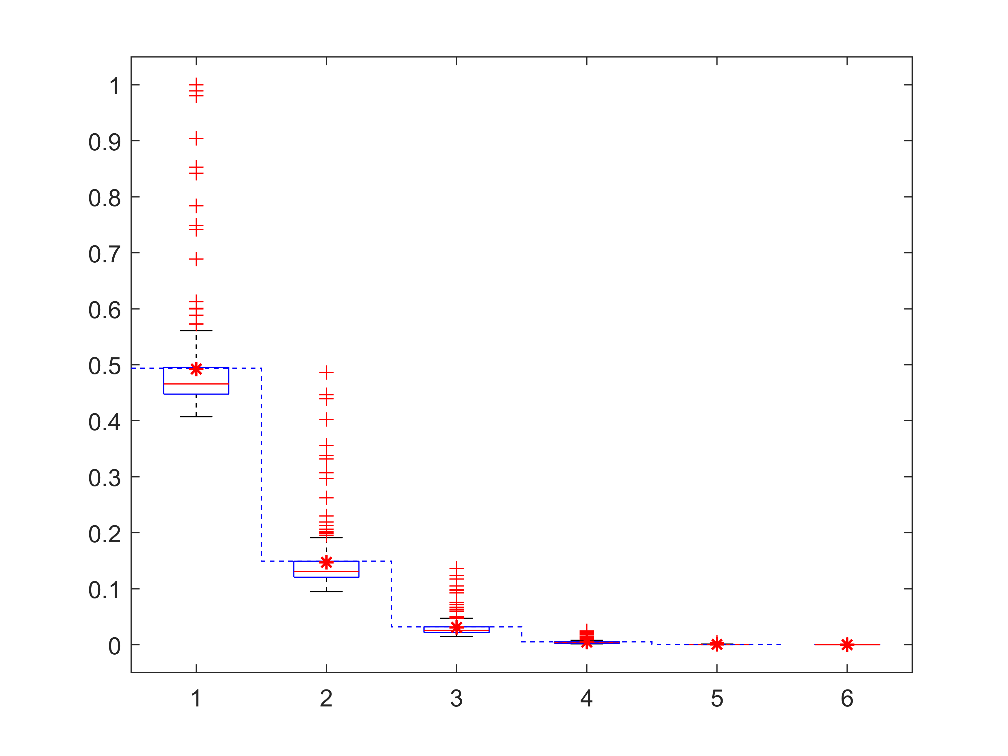
Refer to caption
Figure 3: Random grain model for α=1.3\alpha=1.3, ap=0.005a_{p}=0.005 and c=10​apc=10a_{p}. Boxplots of the estimated volume fraction of the excursion sets of the random grain model, based on 200 independent realizations, {p^λ,k;1≤k≤6}\{\widehat{p}_{\lambda,k};1\leq k\leq 6\} given by (5.1). The red stars indicate the empirical mean value. The dotted blue stairs represent the theoretical values {pk;1≤k≤6}\{p_{k};1\leq k\leq 6\}.

Then, from Theorem 1 and Corollary 1

λν−ν/α(p^λ,k−pk)=λ−ν/α(X^λ,k(A)−EX^λ,k(A))⟶de−μμk−1(k−1)!Lα(A),\lambda^{\nu-\nu/\alpha}(\widehat{p}_{\lambda,k}-p_{k})=\lambda^{-\nu/\alpha}\left(\widehat{X}_{\lambda,k}(A)-\mathrm{E}\widehat{X}_{\lambda,k}(A)\right)\overset{\mathrm{d}}{\longrightarrow}\mathrm{e}^{-\mu}\frac{\mu^{k-1}}{(k-1)!}L_{\alpha}(A), (5.2)

where, recalling (2.8),

Eei​θ​Lα​(A)=exp⁡{i​cΞ​θ​Lebν​(A)​∫ℝ+(ei​θ​x−1)​x−α​𝑑x}.\mathrm{E}\mathrm{e}^{\mathrm{i}\theta L_{\alpha}(A)}=\exp\Big\{\mathrm{i}c_{\Xi}\theta{\rm Leb}_{\nu}(A)\int_{\mathbb{R}_{+}}\big(\mathrm{e}^{\mathrm{i}\theta x}-1\big)x^{-\alpha}\mathrm{d}x\Big\}.

According to (3.9) in chapter XVII of [11], for any a∈(0,1)a\in(0,1), and θ>0\theta>0

∫ℝ+(ei​θ​x−1)x−a−1dx=θaΓ⁡(2−a)a⁡(a−1)e−iπa/2.\int_{\mathbb{R}_{+}}\big(\mathrm{e}^{\mathrm{i}\theta x}-1\big)x^{-a-1}\mathrm{d}x=\theta^{a}\frac{\Gamma(2-a)}{a(a-1)}e^{-i\pi a/2}.

Hence, taking α=1+a\alpha=1+a, one has

iθ∫ℝ+(ei​θ​x−1)x−αdx=θαΓ⁡(2−α)α−1e−iπα/2,i\theta\int_{\mathbb{R}_{+}}\big(\mathrm{e}^{\mathrm{i}\theta x}-1\big)x^{-\alpha}\mathrm{d}x=\theta^{\alpha}\frac{\Gamma(2-\alpha)}{\alpha-1}e^{-i\pi\alpha/2},

from which we deduce that, for all θ∈ℝ\theta\in\mathbb{R},

i​θ​∫ℝ+(ei​θ​x−1)​x−α​𝑑x=|θ|α​Γ⁡(2−α)α−1​cos⁡(π​α/2)​(1−i​sgn​(θ)​tan⁡(π​α/2)).i\theta\int_{\mathbb{R}_{+}}\big(\mathrm{e}^{\mathrm{i}\theta x}-1\big)x^{-\alpha}\mathrm{d}x=|\theta|^{\alpha}\frac{\Gamma(2-\alpha)}{\alpha-1}\cos(\pi\alpha/2)\left(1-i\mbox{sgn}(\theta)\tan(\pi\alpha/2)\right).

Therefore, in view of Definition 1.1.6 of [31], the α\alpha stable random variable Lα​(A)L_{\alpha}(A) follows a stable distribution of parameters α\alpha, β=1\beta=1, δ=0\delta=0 and scale parameter

γ=(cΞ​Lebν​(A)​Γ⁡(2−α)α−1​|cos⁡(π​α/2)|)1/α.\gamma=\left(c_{\Xi}{\rm Leb}_{\nu}(A)\frac{\Gamma(2-\alpha)}{\alpha-1}\left|\cos(\pi\alpha/2)\right|\right)^{1/\alpha}.

Using the Matlab package STBL [34] this will allow us to compare empirical results with the theoretical probability distribution in Figure 4.

Refer to caption Refer to caption Refer to caption
k=1k=1 k=2k=2 k=3k=3
Figure 4: Random grain model for α=1.3\alpha=1.3, ap=0.005a_{p}=0.005 and c=10​apc=10a_{p}. Histograms of the statistic λν−ν/α​λν−ν/α​(p^λ,k−pk)\lambda^{\nu-\nu/\alpha}\lambda^{\nu-\nu/\alpha}(\widehat{p}_{\lambda,k}-p_{k}) for k∈{1,2,3}k\in\{1,2,3\}, based on 200200 independent realizations. The red curves show the theoretical asymptotic probability distributions in view of (5.2).

Next, we consider empirical estimates of the volume fractions defined above along lines parallel to the coordinate axes. We have ν0=1\nu_{0}=1, α0=2​α−1\alpha_{0}=2\alpha-1 and we define

L​p^λ,k:=λ−ν0​X^λ,k​(A∩Hν0)=λ−ν0​Lebν0​({𝒕∈λ​A∩Hν0;X⁡(𝒕)≥k}),L\widehat{p}_{\lambda,k}:=\lambda^{-\nu_{0}}\widehat{X}_{\lambda,k}(A\cap H_{\nu_{0}})=\lambda^{-\nu_{0}}{\rm Leb}_{\nu_{0}}(\{\boldsymbol{t}\in\lambda A\cap H_{\nu_{0}};X(\boldsymbol{t})\geq k\}), (5.3)

as the estimator of the volume fraction computed from a single line of the image.

Refer to caption Refer to caption Refer to caption
horizontal vertical
Figure 5: Left: random grain model for α=1.3\alpha=1.3, ap=0.005a_{p}=0.005 and c=10​apc=10a_{p}. Middle: Observations of the random field along the horizontal line. Right: Observations of the random field along the vertical line.

Then, for α0<2\alpha_{0}<2, taking horizontal or vertical lines (see Figure 5), such that Lebν0​(A∩Hν0)=1{\rm Leb}_{\nu_{0}}(A\cap H_{\nu_{0}})=1, Theorem 3 and Corollary 3 yield

λν0−ν0/α0​(L​p^λ,k−pk)\displaystyle\lambda^{\nu_{0}-\nu_{0}/\alpha_{0}}(L\widehat{p}_{\lambda,k}-p_{k}) =\displaystyle= λ−ν0/α0(X^0,λ,k(A∩Hν0)−EX^0,λ,k(A∩Hν0))\displaystyle\lambda^{-\nu_{0}/\alpha_{0}}\left(\widehat{X}_{0,\lambda,k}(A\cap H_{\nu_{0}})-\mathrm{E}\widehat{X}_{0,\lambda,k}(A\cap H_{\nu_{0}})\right)
⟶d\displaystyle\overset{\mathrm{d}}{\longrightarrow} e−μ​μk−1(k−1)!​Lα0​(A∩Hν0).\displaystyle\mathrm{e}^{-\mu}\frac{\mu^{k-1}}{(k-1)!}L_{\alpha_{0}}(A\cap H_{\nu_{0}}).

The α0\alpha_{0}-stable distribution Lα0​(A)L_{\alpha_{0}}(A) has parameters given by α0\alpha_{0}, β0=1\beta_{0}=1, δ0=0\delta_{0}=0 and

γ0=(c0,Ξ​Lebν​(A)​Γ⁡(2−α0)α0−1​|cos⁡(π​α0/2)|)1/α0.\gamma_{0}=\left(c_{0,\Xi}{\rm Leb}_{\nu}(A)\frac{\Gamma(2-\alpha_{0})}{\alpha_{0}-1}\left|\cos(\pi\alpha_{0}/2)\right|\right)^{1/\alpha_{0}}. (5.4)

In view of (4.13) we may compute, using the Beta function,

∫ℝE⁡(g0​(s)0α)​𝑑s=2α0​∫−11(1−s2)α0/2​𝑑s=22​α0+1​B​(α0+22,α0+22),\int_{\mathbb{R}}\mathrm{E}\left(g^{0}(s)^{\alpha}_{0}\right)\mathrm{d}s=2^{\alpha_{0}}\int_{-1}^{1}(1-s^{2})^{\alpha_{0}/2}\mathrm{d}s=2^{2\alpha_{0}+1}B\left(\frac{\alpha_{0}+2}{2},\frac{\alpha_{0}+2}{2}\right),

and h∞=2​αα0​cαh_{\infty}=2\frac{\alpha}{\alpha_{0}}c^{\alpha} such that we explicitly have

c0,Ξ=22​α0+2​αα0​cα​B​(α0+22,α0+22).c_{0,\Xi}=2^{2\alpha_{0}+2}\frac{\alpha}{\alpha_{0}}c^{\alpha}B\left(\frac{\alpha_{0}+2}{2},\frac{\alpha_{0}+2}{2}\right).

We refer to Figure 6 for estimation results comparable with Figure 3 with only one line extracted.
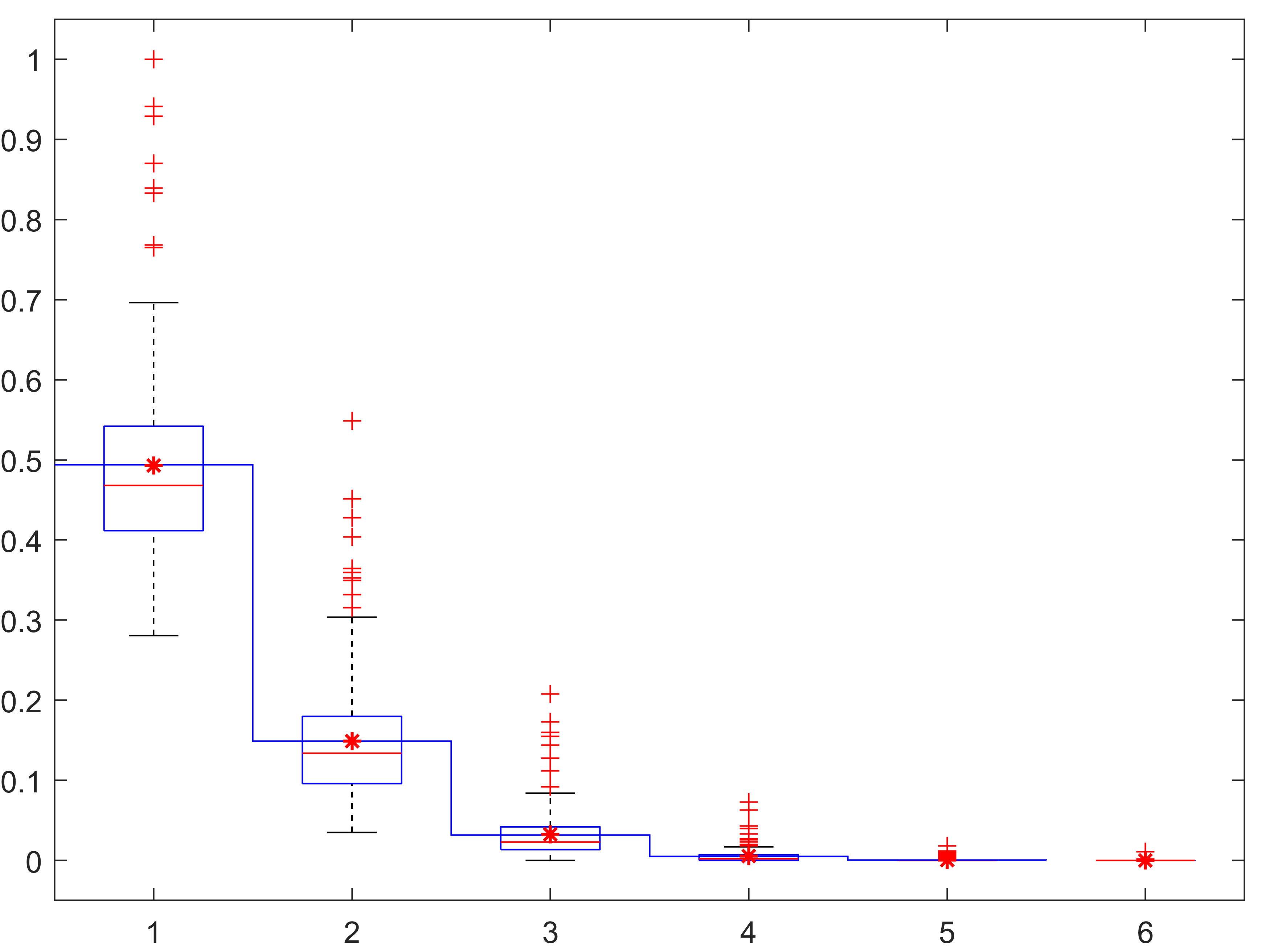
Refer to caption Refer to caption
horizontal vertical
Figure 6: Random grain model for α=1.3\alpha=1.3, ap=0.005a_{p}=0.005 and c=10​apc=10a_{p}. Boxplots of the estimated volume fraction of the excursion sets of the restrictions along lines, based on 200 independent realizations, {Lp^λ,k;1≤k≤6}\{L\widehat{p}_{\lambda,k};1\leq k\leq 6\} given by (5.3). The red stars indicate the empirical mean value. The dotted blue stairs represent the theoretical values {pk;1≤k≤6}\{p_{k};1\leq k\leq 6\}. Left: horizontal lines, right: vertical ones.

In Figure 7 we check the asymptotic behavior and compare with the stable distribution limit obtained for the image.

Refer to caption Refer to caption Refer to caption
k=1k=1 k=2k=2 k=3k=3
Figure 7: Random grain model for α=1.3\alpha=1.3, ap=0.005a_{p}=0.005 and c=10​apc=10a_{p}. Histograms of the statistic λν0−ν0/α0​λν−ν/α​(L^​pλ,k−pk)\lambda^{\nu_{0}-\nu_{0}/\alpha_{0}}\lambda^{\nu-\nu/\alpha}(\widehat{L}p_{\lambda,k}-p_{k}) for k∈{1,2,3}k\in\{1,2,3\}, based on 200200 independent realizations. The red curves show the theoretical asymptotic probability distributions in view of (5.4). The blue curves show the stable probability distributions given by (5.2).

Acknowledgments: This work has been partly supported by the project ANR MISTIC (ANR-19-CE40-0005).

References

  • [1] R. J. Adler. On excursion sets, tube formulas and maxima of random fields. Ann. Appl. Probab., 10(1):1–74, 2000.
  • [2] R. J. Adler and J. E. Taylor. Random fields and geometry. Springer Monographs in Mathematics. Springer, New York, 2007.
  • [3] F. Baccelli, B. Błaszczyszyn, and M. Karray. Random measures, point processes, and stochastic geometry. Inria (hal-02460214v2), 2024.
  • [4] A. Baddeley. A limit theorem for statistics of spatial data. Adv. Appl. Probab., 12:447–461, 1980.
  • [5] H. Biermé and A. Desolneux. Mean geometry for 2d random fields: Level perimeter and level total curvature integrals. Ann. Appl. Probab., 30:561–607, 2020.
  • [6] H. Biermé, O. Durieu, and Y. Wang. Generalized operator-scaling random ball model. ALEA, Lat. Am. J. Probab. Math. Stat., 15:1401–1429, 2018.
  • [7] H. Biermé, A. Estrade, and I. Kaj. Self-similar random fields and rescaled random balls models. J. Theoret. Probab., 23:1110–1141, 2010.
  • [8] L. Breiman. On some limit theorems similar to the arc-sin law. Theory Probab. Appl., 10:323–331, 1965.
  • [9] J.-C. Breton and C. Dombry. Rescaled weighted random ball models and stable self-similar random fields. Stochastic Process. Appl., 119(10):3633–3652, 2009.
  • [10] A. Bulinski, E. Spodarev, and F. Timmermann. Central limit theorems for the excursion set volumes of weakly dependent random fields. Bernoulli, 18(1):100–118, 2012.
  • [11] W. Feller. An introduction to probability theory and its applications, Volume 2, volume 2. John Wiley & Sons, 1991.
  • [12] B. Galerne and R. Lachieze-Rey. Random measurable sets and covariogram realizability problems. Adv. Appl. Probab., 47(3):611–639, 2015.
  • [13] P. Hall. Introduction to the theory of coverage processes. Wiley Ser. Probab. Math. Stat. New York etc.: Wiley, 1988.
  • [14] I. Kaj, L. Leskelä, I. Norros, and V. Schmidt. Scaling limits for random fields with long-range dependence. Ann. Probab., 35:528–550, 2007.
  • [15] I. Kaj and M.S. Taqqu. Convergence to fractional brownian motion and to the telecom process: the integral representation approach. In M.E. Vares and V. Sidoravicius, editors, In and Out of Equilibrium 2, volume 60 of Progress in Probability, pages 383–427. Birkhäuser, Basel, 2008.
  • [16] R. Kulik and P. Soulier. Heavy tailed time series. Springer Ser. Oper. Res. Financ. Eng. New York, NY: Springer, 2020.
  • [17] R. Kulik and E. Spodarev. Long range dependence of heavy-tailed random functions. J. Appl. Probab., 58(3):569–593, 2021.
  • [18] M. Kuronen and L. Leskelä. Hard-core thinnings of germ-grain models with power-law grain sizes. Adv. Appl. Probab., 45(3):595–625, 2013.
  • [19] R. Lachièze-Rey. Normal convergence of nonlocalised geometric functionals and shot-noise excursions. Ann. Appl. Probab., 29(5):2613–2653, 2019.
  • [20] S.N. Lahiri and P.M. Robinson. Central limit theorems for long range dependent spatial linear processes. Bernoulli, 22:345–375, 2016.
  • [21] R. Leipus, V. Pilipauskaitė, and D. Surgailis. Aggregation of network traffic and anisotropic scaling of random fields. Theor. Probab. Math. Statist., 108:77–126, 2023.
  • [22] V. Makogin and E. Spodarev. A short memory condition for infinitely divisible random fields. Stat. Probab. Lett., 221:110385, 2025.
  • [23] S. Mase. Asymptotic properties of stereological estimators. J. Appl. Probab., 19:111–126, 1982.
  • [24] B. Matérn. Spatial variation: stochastic models and their application to some problems in forest surveys and other sampling investigations. Meddelanden Fran Statens Skogsforskningsinstitut, Stockholm, 1960.
  • [25] V. Mattutat. Geometric functionals of polyconvex excursion sets of Poisson shot noise processes. Ann. Appl. Probab., 36(4):3757–3791, 2026.
  • [26] T. Mikosch, S. Resnick, H. Rootzén, and A. Stegeman. Is network traffic approximated by stable lévy motion or fractional brownian motion? Ann. Appl. Probab., 12:23–68, 2002.
  • [27] I. Molchanov and D. Stoyan. Asymptotic properties of estimators for parameters of the boolean model. Adv. Appl. Probab., 26:301–323, 1994.
  • [28] V. Pilipauskaitė and D. Surgailis. Anisotropic scaling of random grain model with application to network traffic. J. Appl. Probab., 53:857–879, 2016.
  • [29] V. Pilipauskaitė and D. Surgailis. Fractional operators and fractionally integrated random fields on ℤν\mathbb{Z}^{\nu}. Fractal Fract., 8:353, 2024.
  • [30] S.I. Resnick. Heavy tailed phenomena. Probabilistic and statistical modeling. Springer Ser. Oper. Res. Financ. Eng. 2007.
  • [31] G. Samorodnitsky and M. S Taqqu. Stable non-Gaussian random processes: stochastic models with infinite variance. CRC press, 1994.
  • [32] D. Stoyan, W.S. Kendall, and J. Mecke. Stochastic Geometry and Its Applications. Akademie-Verlag, Berlin, 1989.
  • [33] D. Surgailis. Scaling limits of nonlinear functions of random grain model, with application to burgers’ equation. Stochastic Process. Appl., 174:104390, 2024.
  • [34] M. Veillette. STBL: Matlab toolbox for stable distributions. https://math.bu.edu/people/mveillet/html/stable.html, 2012.