Abstract
This chapter provides a pedagogical introduction to theoretical studies of hadrons based on the fundamental theory of strong interactions - Quantum ChromoDynamics. A perturbative expansion in the strong coupling is not applicable at hadronic energy scales. Lattice Quantum Chromodynamics is the formulation of the fundamental theory on a discrete space-time grid, which enables first-principles, systematically improvable, numerical simulations of strong interaction physics. This chapter explains how the masses of strongly stable and strongly decaying hadrons are determined. The strongly decaying hadrons have to be inferred from the corresponding scattering processes. Therefore, one of the main aims is to describe how the scattering amplitudes are extracted from a lattice simulation. The examples of spectra, widths, and scattering amplitudes are shown for conventional as well as exotic hadrons.
keywords
hadrons\sepspectroscopy\sepQCD\seplattice QCD \sepscatteringChapter 0 Lattice QCD calculations of hadron spectroscopy
Chapter Article tagline: update of previous edition, reprint.
Objective
The objective is to learn how the following physics problems have been or can be addressed:
- •
Masses of proton, neutron, and other hadrons are not just experimentally measurable quantities, but they have been theoretically determined from the fundamental theory of the strong interactions - QCD.
- •
Masses and lifetimes have been reliably calculated for a number of hadronic resonances, which strongly decay via one channel.
- •
Most of the conventional and exotic hadrons strongly decay to several final states, and some of these have already been addressed ab initio. The presented approach makes it clear why this is a challenging task.
- •
1 Introduction
Strong interactions are the strongest among all four fundamental interactions and are responsible for binding the quarks to color-neutral hadrons. Conventional hadrons have minimal valence quark content (mesons) and (baryons). In the past two decades, around thirty candidates for exotic hadrons with minimal valence quark content (tetraquarks), (pentaquarks), and (hybrids) have been discovered in experiments [6]. The binding mechanisms responsible for the existence of these multi-quark states represent an important open question.
The main aim of hadron spectroscopy is to determine hadron masses and improve our understanding of emerging mass patterns. One of the main challenges is that most of the known hadrons, and in particular all the experimentally observed exotic hadrons, are hadronic resonances. These are metastable states that decay quickly to lighter hadrons via the strong interaction, either only to one final state or to several final states . An important aim for resonances is to determine their decay width or equivalently the lifetime , branching ratios for various final states, and lineshapes as a function of invariant masses .
This chapter aims at a pedagogical introduction on how to theoretically determine the physics observables listed in the previous paragraph from first-principle lattice QCD, and provide a few pedagogical examples. The only interaction at play will be the strong interactions described with , while electro-weak interactions will be neglected. Let us first briefly review how difficult it is to study a given hadron, where the difficulty increases from bottom to top as illustrated in Figure 1(b):
- •
Hadrons that are stable with respect to strong decay and lie significantly below the lowest decay threshold are the most straightforward.
- •
Hadrons that can decay via single channel or hadrons that reside slightly below threshold have to be inferred from the scattering sketched in Figure 1(c). This already presents a more challenging theoretical problem since the scattering amplitude has to be extracted, where is the center-of-momentum energy. The hadronic states correspond to the pole singularities of in the complex plane. The pole position is related to hadron mass and width, while is related to the experimental lineshape. The ab initio theory study of the scattering amplitudes is, therefore, a prime subject of this chapter.
- •
The hadrons residing above two or more thresholds and decaying via several decay channels represent an even more challenging problem. An example of a resonance that decays via channels (channel ) and (channel ) is sketched in Figure 1(d). The energy dependence of the scattering matrix () with elements , and are of prime theoretical and experimental interest in this case. All elements of the scattering matrix have the pole at the energy where vanishes, and the pole position is again related to the mass and the width of the state.
- •
The hadrons that can strongly decay also to the final states with more than two hadrons are even more challenging, and their study goes beyond this chapter. The past few years have evidenced impressive progress on the formalisms and on actual numerical lattice QCD results for three-hadron scattering amplitudes from the lattice.
The experimental determination of resonance parameters by measuring the cross-section for scattering follows a similar strategy as described above. However, the experimental determination of resonance parameters for many other resonances is somewhat different since many hadrons (, ,..) quickly decay via the electro-weak interaction. In these cases, the initial state in Figure 1(c) can not be realized in an experiment, and resonances are produced via various other production mechanisms. The experimental observables depend on the underlying scattering amplitude also in this case, which calls for their theoretical determination.
The hadrons emerge from the strong interaction between quarks at energy scales where non-perturbative effects dominate. Consequently, a perturbative expansion in the QCD gauge coupling is inapplicable. Lattice QCD is a widely used non-perturbative method with systematically improvable uncertainties. It is based directly on the QCD Lagrangian , where the only free parameters are quark masses and the strong coupling . The spectroscopic properties of hadrons are determined from correlation functions . Lattice QCD is based on the Feynman path integral approach, where the correlation function is as an expectation value of correlation functions obtained by functional integration over all gluon and quark fields
| (1) |
where is the correlation function for a given configuration of gluon and quark fields. Each field configuration is weighted by the factor in the case of the Minkowski space-time. Lattice simulations employ Euclidean time , and the corresponding weight is real. These path integrals are evaluated via the numerical evaluation on a discretized and Euclidean space-time of finite volume sketched in Figure 1(a) [7]. Reliable physics predictions should be based on simulations at several lattice spacings and several spatial volumes , followed by the continuum and infinite volume extrapolations and . Lattice QCD can explore how the properties of hadrons depend on the quark masses of each quark flavor. This is a very valuable handle used to investigate the binding mechanisms that are responsible for their existence.
Practically all physics observables mentioned above can be calculated from eigen-energies of the QCD Hamiltonian on the finite lattice, as argued in the reminder of this chapter. This applies also to the scattering amplitude derived in Section 4. The next section introduces how to determine eigen-energies from the so-called two-point correlation functions , which are, in turn, evaluated via the path integral above.

2 Eigen-energies from a lattice simulation
Spectroscopic information for a hadron that resides below, near, or above threshold is commonly extracted from the discrete set of energies of QCD eigenstates on a finite-volume lattice. These are determined from the two-point correlation functions , where is the vacuum, creates a hadron system with quantum numbers of interest, and annihilates it after time .
The operators are built out of quark and gluon field operators and should have the same quantum numbers as the system of interest: these are typically flavor quantum numbers, total momentum and the quantum numbers related to parity and spin11 1 A lattice with a finite spatial extent has a reduced symmetry compared to an infinite-volume continuum. This means that instead of , the relevant quantum number is an irreducible representation of the appropriate point group, for example, a cubic group in the case of momentum zero.. Care must be taken to ensure that operators have appropriate structures to effectively overlap with the eigenstates of interest. They create/annihilate the eigenstates of interest, as well as, in principle, all other eigenstates with a given quantum number. Examples of operators in the meson sector with conventional or exotic quark content are
where quarks fields carry various flavors and apply at the same , except in the last operator. There, each meson is separately projected to a given momentum with and . Typical simulations in Sections 4 and 5 employ around operators with a given quantum number at the source and the sink, and the resulting correlation matrix is of size .
The dependence of the correlation function on is obtained upon insertion of the complete set of QCD eigenstates on a finite volume of the lattice
| (2) |
Here the eigenvalue equation and the evolution of operators on Euclidean time were employed. The overlap of a given eigenstate and operator provides valuable qualitative information.
As an example, the correlation function for a system with kaon quantum numbers and total momentum is calculated with the path integration (1) using the point-like creation operator and annihilation operator as illustrated in Figure 1(e)
| (3) |
The right-hand side follows after the path integration over the quark fields in . According to the Wick theorem, the path integral over quark fields renders the product of quark propagators and for a theory with degenerate quarks (see Section 5.1 of [7]). For kaon correlation function, the integrand contains the kaon correlator on a given gluon field configuration, which is a traced product of -quark and -quark propagators between space-time points and and appropriate matrices, as illustrated in Figure 1e. The quark propagator on a given background gluon field is obtained by inverting the Dirac matrix on the lattice, which is a discretized and Euclidean version of the continuum operator . is a large matrix of typical size with , where and are dimensions of color and spinor spaces, respectively. Therefore, its inverse and determinant are among the numerically intensive parts of the calculation. The final correlator is obtained by summing the correlator over the gluon field configurations , each weighted by [7]. In practice, the ensemble of gauge configurations is prepared such that a given configuration is generated with a probability proportional to .
The study of a hadron with mass requires the extraction of all eigenstates with the same quantum numbers and energies . In order to extract the energies and overlaps via relation (2), the correlation matrix with operators is calculated. Then the eigenvalue problem is solved for times larger then a fixed reference time [8]. Let us show that the time-dependence of the eigenvalues renders via at large . Suppose is large enough that only the lowest eigenstates contribute to the correlation function (2) in the time region between and , i.e. . Then the vectors satisfying can be found, which implies that decays as a single-exponential. The eigenvalue, therefore, also decays as a single exponential with the energy of interest. In practice, are determined from one-exponential or two-exponential fits at large enough since typically more than eigenstates contribute in the time region between and . The described and widely used generalized eigenvalue approach (GEVP) also allows the determination of the overlaps .
3 Strongly-stable hadrons well below threshold
Among the vast number of hadrons, only a handful do not decay via the strong interaction. In the absence of electroweak interactions, the stable hadrons are the lowest-lying states of a given flavor content: , , , , , , , , , , etc. Their masses are obtained from ground state energies as after these energies are extrapolated to zero lattice spacing and large volume. The ground state energies are calculated from the two-point correlation functions (2). A number of lattice QCD simulations have already determined masses of such hadrons with sub-percent statistical precision and with all systematic uncertainties quantified or removed. The lattice results for the masses of proton, neutron, and other conventional hadrons in Figure 2 [9, 10] show good agreement with the experiment.
Most of the exotic hadrons can strongly decay. Two exceptions are tetraquarks and with that are expected to lie significantly below thresholds. Their masses have been determined from the ground state energy, and their binding energies increase with increasing and decreasing , as shown in Figure 3 [11].


4 Hadrons from one-channel scattering
Most hadrons are hadronic resonances that decay via the strong interaction. In particular, nearly all experimentally discovered exotic hadrons decay strongly. Such states are not asymptotic states of QCD, and their existence has to be inferred from the amplitude for the scattering illustrated in Figure 4(a). Let us consider the simplest case of a single-channel scattering that is completely dominated by the partial wave . The conservation of probability implies that -matrix can be expressed in terms of a phase shift
| (4) |
where is the on-shell three momentum of the scattering particles in the center-of-momentum frame22 2 Various normalizations of are used in the literature. Here is of Ref. [12], adapted by a factor of 2 suited for the scattering of non-identical particles in Section 1. . The cross-section is proportional to , so the energy dependence of is the main quantity of interest.
A resonance corresponds to a pole of the scattering amplitude away from the real axes, as sketched in Figure 4(b). Bound state and virtual state correspond to a pole at below threshold, therefore at real negative . The bound state pole at positive imaginary is related to an asymptotic bound state with decreasing wave-function outside the region of interaction. The virtual state pole is not related to an asymptotic state as its wave function increases as outside the region of interaction. Both bound and virtual states lead to a significant enhancement of the scattering rate above the threshold if the poles are located only slightly below the threshold.


1 Relation between finite-volume eigen-energies and infinite-volume scattering amplitude
The most widely applied and rigorous method to extract the scattering matrix from ab-initio lattice QCD simulations is the so-called Lüscher formalism [13, 12]. In order to determine the amplitude for scattering in a channel with certain quantum numbers, the eigen-energies of a system with these quantum numbers have to be calculated from lattice QCD. The Lüscher formalism rigorously relates the discrete eigenenergy of the system in a finite volume, sketched in Figure 4(c), with the infinite volume scattering matrix at the same
| (5) |
An explicit example of this relation is derived below and provided in Eq. (12) for the simplest case of scattering with the periodic boundary conditions, , and total momentum zero. The generalized relation for the scattering of particles with arbitrary spin and partial wave is provided in Eq. (22) of [14]. Lattice studies aim to extract a large number of eigen-energies in order to constrain the scattering amplitude at various energies . Several lattice sizes and various total momenta are employed for this purpose.
One-dimensional quantum mechanics
The relation between eigen-energies and the scattering amplitude can be most easily derived in one-dimensional quantum mechanics as illustrated in Figure 5(a). In the absence of potential, the wave function equals with due to the periodic boundary condition. For a non-zero potential of finite range, the wave function acquires a phase shift outside the region of potential, and the momentum is modified to
| (6) |
in order to still satisfy the periodic boundary conditions and . The finite volume accompanied by certain boundary conditions, therefore, implies a relation between and for an interacting system.
Derivation of Lüscher’s relation in QFT
Now let’s turn to the finite-volume eigen-energies in Quantum Field Theory. The non-interacting (ni) eigenenergies of two hadrons in a finite box with periodic boundary conditions represent a valuable reference point (which will be denoted by lines in the spectrum plots)
| (7) |
The energies are modified due to the interactions between two hadrons, and the energy shifts depend on the scattering amplitudes.
In order to derive the relation between eigen-energies and the scattering amplitude at the same energy in QFT, I present essential steps from Ref. [12], simplified to the scattering of two non-identical scalar particles in partial wave and total momentum . The scattering amplitude is given by the infinite sum of diagrams presented in Figure 5(b). The lines represent the dressed renormalized scalar propagators, and the kernel is the sum of two-particle irreducible diagrams in the s-channel illustrated in Figure 5(c).

We will relate energy and scattering amplitude via the finite-volume correlation function that is Fourier transformed from Minkowski time to energy. On one hand, it depends on the eigen-enegies as
| (8) |
being singular at each . On the other hand, is given by the infinite sum of diagrams with kernel in Figure 5(d), and our aim is to express in terms of the scattering amplitude. The important contribution to will be represented by the intermediate particles that can go on-shell, propagate to the spatial boundary, and render significant finite-volume effects, while the exponentially suppressed finite-volume corrections will be neglected [12].
Correlator features the finite-volume loop in Figure 5(f), which can be decomposed into the sum of the infinite-volume loop and the finite-volume correction . The correction arises from the difference between the integral over the loop momenta and the sum over the discrete values in a periodic box :
| (9) |
Here and represent any of , or , and they depend only on the magnitude of the momentum in case of the s-wave scattering. The integral is evaluated by applying the Cauchy theorem. The contour is closed around the lower-half plane and encapsulates the poles at and . The residue of the integrand at is non-singular in the whole region of interest. This renders only the neglected exponentially suppressed contribution since for non-singular integrand according to the Poisson summation formula. The residue of the integrand (9) at the first pole is proportional to and is singular only when . This occurs when both particles are on-shell, and the loop momentum is equal to the on-shell momentum . The difference between the finite sum and the integral for a singular integrand is not exponentially suppressed, and renders an important contribution
| (10) |
The above equation introduces the kinematical function , which will appear in the final Lüscher’s relation, and matches the more general defined in Eq. (48) of Ref. [12]. The same reference also provides a useful relation to evaluate , which is independent of the regularization since the ultra-violet part cancels. The kernels and in (10) are evaluated at the on-shell momentum as dictated by the pole . This separation between the on-shell quantities and the kinematical function will allow us to express the correlator in terms of the on-shell scattering amplitude .
The finite-volume loop, expressed as a sum , is inserted in place of each loop in the finite-volume correlator in Figure 5(d). A proliferation of terms for is obtained. They can be combined as shown in Figure 5(e), as the reader can check by drawing some examples in this sum. The first term contains only and corresponds to the correlation function in infinite volume . The other diagrams can be expressed in terms of , the dressed overlaps to operators and the infinite volume scattering amplitude , all defined in Figure 5. The resulting finite volume correlator
| (11) |
is now expressed in terms of the on-shell infinite-volume scattering amplitude . This comes about since the finite-volume correction to the loop in (10) depends on the on-shell quantities, which follows from the dominant role of on-shell particles in the loop. Poles of appear when the denominator vanishes and where according to (8). This leads to the Lüscher’s relation between and
| (12) |
which applies when is equal to the eigen-energy . The kinematical function is given in Eq. (48) of [12]. The lattice eigen-energy , therefore, directly renders the scattering amplitude at the same energy.


2 Examples
Resonances and
In order to illustrate how resonances are studied in lattice QCD, the study of scattering in the -meson channel with from Ref. [15] is presented in Figure 6. The finite-volume energies of an interacting two-pion system on a single volume with fm and MeV are shown for total momenta and . The energies are shifted with respect to the non-interacting energies (represented by lines), which implies non-zero interaction between pions. Each energy renders the scattering amplitude and the scattering phase shift at that energy , as illustrated by circles of various colors: the underlying relation for is given in Eq. (12)33 3 This relation applies here although this is scattering with . . The same lattice study extracted the eigen-energies also for higher total momenta up to , thereby probing this two-pion system and the corresponding phase shift at further kinematical points . All points are collected in the plot on the right, where the phase shift features a clear resonance shape and is described well with a Breit-Wigner form44 4 The factor comes from normalization choice for in Eq. (4).
| (13) |
The phase shift rises through at the resonance mass MeV which is close to the MeV in Nature. The width is smaller than in Nature due to the smaller phase space for decay at heavier-than-physical pions, but the coupling that parametrizes the width has the value close to the value in Nature.
A large number of lattice collaborations have already established the resonances and at a variety of and quark masses, including the physical ones. Figure 7 displays recent results employing RBC/UKQCD ensembles with the physical quark masses [16], using Breit-Wigner parametrization (13) and verifying good agreement with experiment for the phase shifts and the pole position .


Heavy-light scalar mesons
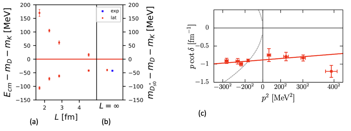
The scalar charm-strange meson is a vanilla example of a bound state. It was experimentally discovered about MeV below threshold and is strongly stable in the isospin limit . The scattering phase shift in partial wave was extracted at eight values of energies, obtained from four spatial volumes and applying Lüscher’s relation (12) [17], all shown in Figure 8. As momenta and phase shifts are imaginary below the threshold, it is customary to present the real quantity . The scattering amplitude (4) features a bound state pole below threshold, where (red line) intersects with (dashed gray line) for positive imaginary momenta . The position of this bound state in pane (b) agrees well with the experimental mass of .
The charmed scalar mesons would form a flavor anti-triplet with according to the quark model. However, a new paradigm is supported by a number of studies using effective field theories, lattice simulations as well as re-analysis of experimental data, for example [19, 20, 21, 18]. According to this paradigm, the spectrum features as well as Fock components. The latter decomposes to the multiplets in the flavor limit. The attractive interactions within the anti-triplet and the sextet suggest the existence of hadrons indicated by circles in Figure 9, with two pairs of poles for charmed mesons. The spectrum of charmed scalar mesons by the Hadron Spectrum collaboration shows members of the triplet and sextet at three different pion masses, as summarized in [18]. The state indicated by red carries an exotic flavor quantum number. All these hadrons have been extracted from poles of for the scattering of charmed and light mesons with the Lüscher’s formalism.

Doubly heavy tetraquarks and
The doubly charm tetraquark with and was experimentally discovered less than MeV below threshold by LHCb [23]. Several recent lattice simulations have extracted the scattering amplitude in the kinematics where is stable, and all simulations indeed found the pole near the threshold. The quark mass dependence of the pole position was investigated in [22], where scattering amplitude was extracted from finite-volume energies by combining Lüscher approach and Effective Field Theory to incorporate the effects of the so-called left-hand cut [24]55 5 Lüscher’s relation namely does not apply in the region below threshold where pion comes on-shell in u-channel exchange (in kinematics when ).. The pole transitions between a resonance, virtual state, and bound state when is increased or when is decreased, as shown in Figures 10(a,b). Such a pole trajectory is consistent (but does not uniquely imply) with interacting through the potential sketched in Figure 10(c), which is almost independent of and becomes more attractive with decreasing [22]. This is roughly in line with the expectation from the exchange of light mesons between and . The current understanding of this interesting state as of 2024 will surely improve with further studies.

Nucleon-nucleon scattering
The scattering of nucleons is particularly challenging due to the signal-to-noise problem. In order to extract the amplitude for the scattering of proton and neutron in the deuteron channel, the eigen-energies of this system with have been determined at zero total momentum (shown in Figure 12a) and also at other total momenta. The generalization of the Lüscher’s relation renders for partial wave in Figure 12a, in the approximation where is neglected. The scattering amplitude (4) has a virtual state pole where . This is realized for where the line intersects with the red dashed line representing . This simulation at MeV confirms the attraction between proton and neutron, which is, however, not large enough to render a deutron bound state, but is responsible for a near-threshold virtual state. Different colors correspond to simulations at different lattice spacings , which emphasizes significant discretization effects for this channel.


5 Hadrons from coupled-channel scattering
Most resonances lie above several thresholds and decay to several final states via the strong interaction. Light-meson resonances and that feature in the scattering of three coupled channels are shown in Figure 13 [30]. The information on the scattering is again obtained from the finite volume eigen-energies, where the interacting two-meson states , , and feature in the spectra, shown on the left. The scattering is described with scattering matrix, where each element depends on the energy. The Lüscher’s equation for one-channel (12) generalizes for the case of three coupled channels with spinless particles in partial wave to
| (14) |
and it relates and when is lattice eigen-energy. Here, are the same kinematical functions as for one-channel scattering [12], and they depend on the masses of the scattering particles in channel . For a given lattice eigen-energy , the determinant equation is one equation for six unknown . It is, therefore, customary to parametrize the energy dependence of all in terms of a few unknown parameters . These parameters are fitted so that lattice eigen-energies are best reproduced with the prediction of the Lüscher’s equation for (14). The resulting scattering matrix in Figure 13 is constrained by the spectra with total momentum zero, as well as other total momenta that are not shown. Two channels and are found to be significantly coupled for and almost uncoupled for , while coupling to is small in both cases. The poles are related to scalar and tensor resonances and , while pole is below threshold at this pion mass.
6 Hadrons from static potentials
Hadronic systems that contain two heavy quarks, i.e. or , and additional light degrees of freedom (gluons and/or light quarks ), can be addressed via the Born-Oppenheimer approximation since the velocities of heavy quarks are much smaller than those of the light degrees of freedom. Let’s consider a system with in Figure 12(c), where the eigen-energies of a system with a static pair of quarks at a fixed distance were determined in [29]. These are called the static energies and are obtained from the correlation functions as described in Section 2 with the sole exception that spatial positions of heavy quarks are fixed in the operator and the propagator. The static eigen-energies provide the potential between and since the kinetic energies of the static mesons are zero. The extracted potential in Figure 12(c) shows significant attraction at explored distances . The potential needs to be extrapolated towards and large , which can be done reliably if its analytic form is known. The scattering amplitudes and possible existence of bound states or resonances are then explored via the Schrödinger equation like in non-relativistic quantum mechanics. This renders the bound state with the binding energy MeV with respect to threshold [29]. The formalism for a great variety of exotic channels is worked out in Ref. [31].
7 Hadrons and potentials from HAL QCD approach
Eigen-energies represent the main quantity extracted from lattice simulations in the previous sections. On the other hand, the HAL QCD approach is based on extracting the Bethe-Salpeter wave function of an eigenstate directly from lattice QCD. The wave function of two scalars within an eigenstate is defined as and illustrated in Figure 12(b) [32]. The HAL QCD collaboration investigates two-hadron systems, where the equal-time Bethe-Salpeter wave function is analogously defined as
| (15) |
Here is a two-hadron eigenstate with energy , are single-hadron operators and spins of hadrons are omitted for simplicity. The wave-function of the ground state can be determined from the large-time behavior of the correlator [28]66 6 In practice, HAL QCD uses a slightly different method to extract from - the so-called so-called time-dependent method.
| (16) |
where is a source operator that creates two-hadron system at time .
The HAL QCD approach relates the wave function to the potential between two hadrons. Within the relativistic theory, this approach renders the so-called non-local potential . Its precise definition goes beyond this introductory text, but it is discussed in numerous HAL QCD papers, for example, in review [28]. The local and central part of the potential in the case of a nucleon-nucleon system in the deuteron channel is presented in Figure 12(b). Here the standard nucleon operators are employed [27, 28]. The potential is repulsive at short distances, attractive at medium and long distances, and does not render a deuteron bound state at MeV. This agrees with the absence of the deuteron bound state at MeV in the study employing the Lüscher’s method shown in Figure 12(a) [26]. The deuteron bound state is expected to emerge once the pion mass is decreased towards the physical pion mass, in which case the lattice results are currently too noisy to render a reliable conclusion.
8 Conclusions
Experiments have provided great discoveries of new conventional hadrons as well as around thirty exotic hadrons. I have presented the theoretical challenge to understand the spectroscopic properties of various hadron sectors from ab initio lattice QCD. This approach yields masses of hadrons that are strongly stable, as well as hadrons that are slightly below the strong decay threshold or decay strongly via one decay channel. The theoretical challenge increases with the number of open decay channels. It seems impossible to address the high-lying states like with current lattice methods, while many interesting physics conclusions are already available for certain lower-lying states.
Acknowledgments: I would like to gratefully thank Christine Davies, Takumi Doi, Sara Collins, Felix Erben, Jeremy Green, Feng-Kun Guo, Tetsuo Hatsuda, Jamie Hudspith, Nelson Pitanga Lachini, Luka Leskovec, Yan Lyu, William Parrott, Stefan Meinel and M. Padmanath. Support by Slovenian Research Agency ARIS for funding programme P1-0035 is acknowledged.
References
- [1] N. Brambilla, S. Eidelman, C. Hanhart, A. Nefediev, C.-P. Shen, C. E. Thomas, A. Vairo, and C.-Z. Yuan, “The states: experimental and theoretical status and perspectives,” Phys. Rept. 873 (2020) 1–154, arXiv:1907.07583 [hep-ex].
- [2] P. Bicudo, “Tetraquarks and pentaquarks in lattice QCD with light and heavy quarks,” Phys. Rept. 1039 (2023) 1–49, arXiv:2212.07793 [hep-lat].
- [3] J. Bulava et al., “Hadron Spectroscopy with Lattice QCD,” in Snowmass 2021. 3, 2022. arXiv:2203.03230 [hep-lat].
- [4] R. A. Briceno, J. J. Dudek, and R. D. Young, “Scattering processes and resonances from lattice QCD,” Rev. Mod. Phys. 90 no. 2, (2018) 025001, arXiv:1706.06223 [hep-lat].
- [5] A. D. Hanlon, “Hadron spectroscopy and few-body dynamics from Lattice QCD,” PoS LATTICE2023 (2024) 106, arXiv:2402.05185 [hep-lat].
- [6] Particle Data Group Collaboration, S. Navas et al., “Review of particle physics,” Phys. Rev. D 110 no. 3, (2024) 030001.
- [7] C. Gattringer and C. B. Lang, Quantum chromodynamics on the lattice, vol. 788. Springer, Berlin, 2010.
- [8] M. Luscher and U. Wolff, “How to Calculate the Elastic Scattering Matrix in Two-dimensional Quantum Field Theories by Numerical Simulation,” Nucl. Phys. B 339 (1990) 222–252.
- [9] BMW Collaboration, S. Durr et al., “Ab-Initio Determination of Light Hadron Masses,” Science 322 (2008) 1224–1227, arXiv:0906.3599 [hep-lat].
- [10] R. J. Dowdall, C. T. H. Davies, T. C. Hammant, and R. R. Horgan, “Precise heavy-light meson masses and hyperfine splittings from lattice QCD including charm quarks in the sea,” Phys. Rev. D 86 (2012) 094510, arXiv:1207.5149 [hep-lat].
- [11] B. Colquhoun, A. Francis, R. J. Hudspith, R. Lewis, K. Maltman, and W. G. Parrott, “Improved analysis of strong-interaction-stable doubly bottom tetraquarks on the lattice,” Phys. Rev. D 110 no. 9, (2024) 094503, arXiv:2407.08816 [hep-lat].
- [12] C. h. Kim, C. T. Sachrajda, and S. R. Sharpe, “Finite-volume effects for two-hadron states in moving frames,” Nucl. Phys. B 727 (2005) 218–243, arXiv:hep-lat/0507006.
- [13] M. Luscher, “Two particle states on a torus and their relation to the scattering matrix,” Nucl. Phys. B 354 (1991) 531–578.
- [14] R. A. Briceno, “Two-particle multichannel systems in a finite volume with arbitrary spin,” Phys. Rev. D 89 no. 7, (2014) 074507, arXiv:1401.3312 [hep-lat].
- [15] C. Alexandrou, L. Leskovec, S. Meinel, J. Negele, S. Paul, M. Petschlies, A. Pochinsky, G. Rendon, and S. Syritsyn, “-wave scattering and the resonance from lattice QCD,” Phys. Rev. D 96 no. 3, (2017) 034525, arXiv:1704.05439 [hep-lat].
- [16] P. Boyle, F. Erben, V. Gülpers, M. T. Hansen, F. Joswig, M. Marshall, N. P. Lachini, and A. Portelli, “Light and Strange Vector Resonances from Lattice QCD at Physical Quark Masses,” Phys. Rev. Lett. 134 no. 11, (2025) 111901, arXiv:2406.19194 [hep-lat].
- [17] G. S. Bali, S. Collins, A. Cox, and A. Schäfer, “Masses and decay constants of the and from lattice QCD close to the physical point,” Phys. Rev. D 96 no. 7, (2017) 074501, arXiv:1706.01247 [hep-lat].
- [18] Hadron Spectrum Collaboration, J. D. E. Yeo, C. E. Thomas, and D. J. Wilson, “DK/D scattering and an exotic virtual bound state at the SU(3) flavour symmetric point from lattice QCD,” JHEP 07 (2024) 012, arXiv:2403.10498 [hep-lat].
- [19] E. E. Kolomeitsev and M. F. M. Lutz, “On Heavy light meson resonances and chiral symmetry,” Phys. Lett. B 582 (2004) 39–48, arXiv:hep-ph/0307133.
- [20] M.-L. Du, M. Albaladejo, P. Fernández-Soler, F.-K. Guo, C. Hanhart, U.-G. Meißner, J. Nieves, and D.-L. Yao, “Towards a new paradigm for heavy-light meson spectroscopy,” Phys. Rev. D 98 no. 9, (2018) 094018, arXiv:1712.07957 [hep-ph].
- [21] M. Albaladejo, P. Fernandez-Soler, F.-K. Guo, and J. Nieves, “Two-pole structure of the ,” Phys. Lett. B 767 (2017) 465–469, arXiv:1610.06727 [hep-ph].
- [22] S. Collins, A. Nefediev, M. Padmanath, and S. Prelovsek, “Toward the quark mass dependence of Tcc+ from lattice QCD,” Phys. Rev. D 109 no. 9, (2024) 094509, arXiv:2402.14715 [hep-lat].
- [23] LHCb Collaboration, R. Aaij et al., “Study of the doubly charmed tetraquark ,” Nature Commun. 13 no. 1, (2022) 3351, arXiv:2109.01056 [hep-ex].
- [24] M.-L. Du, A. Filin, V. Baru, X.-K. Dong, E. Epelbaum, F.-K. Guo, C. Hanhart, A. Nefediev, J. Nieves, and Q. Wang, “Role of Left-Hand Cut Contributions on Pole Extractions from Lattice Data: Case Study for Tcc(3875)+,” Phys. Rev. Lett. 131 no. 13, (2023) 131903, arXiv:2303.09441 [hep-ph].
- [25] C. Alexandrou, J. Finkenrath, T. Leontiou, S. Meinel, M. Pflaumer, and M. Wagner, “Shallow Bound States and Hints for Broad Resonances with Quark Content b¯c¯ud in B-D¯ and B*-D¯ Scattering from Lattice QCD,” Phys. Rev. Lett. 132 no. 15, (2024) 151902, arXiv:2312.02925 [hep-lat].
- [26] Baryon Scattering (BaSc) Collaboration, J. R. Green, A. D. Hanlon, P. M. Junnarkar, and H. Wittig, “Nucleon-nucleon scattering from distillation,” PoS LATTICE2022 (2023) 200, arXiv:2212.09587 [hep-lat].
- [27] HAL QCD Collaboration, N. Ishii, “Baryon-baryon Interactions from Lattice QCD,” PoS CD12 (2013) 025.
- [28] S. Aoki and T. Doi, Lattice QCD and Baryon-Baryon Interactions, pp. 1–31. 2023. arXiv:2402.11759 [hep-lat].
- [29] European Twisted Mass Collaboration, P. Bicudo and M. Wagner, “Lattice QCD signal for a bottom-bottom tetraquark,” Phys. Rev. D 87 no. 11, (2013) 114511, arXiv:1209.6274 [hep-ph].
- [30] R. A. Briceno, J. J. Dudek, R. G. Edwards, and D. J. Wilson, “Isoscalar scattering and the mesons from QCD,” Phys. Rev. D 97 no. 5, (2018) 054513, arXiv:1708.06667 [hep-lat].
- [31] M. Berwein, N. Brambilla, A. Mohapatra, and A. Vairo, “Hybrids, tetraquarks, pentaquarks, doubly heavy baryons, and quarkonia in Born-Oppenheimer effective theory,” Phys. Rev. D 110 no. 9, (2024) 094040, arXiv:2408.04719 [hep-ph].
- [32] N. Nakanishi, “A General survey of the theory of the Bethe-Salpeter equation,” Prog. Theor. Phys. Suppl. 43 (1969) 1–81.