跳到论文正文
W Papers独立论文阅读器 arXiv:2505.08982 论文正文 计算阅读时间 · 0%
引用这篇论文根据当前论文元数据生成,正式投稿前建议核对。


License: CC BY-NC-ND 4.0
arXiv:2505.08982v1 [cs.LG] 13 May 2025

Model-free Online Learning for the Kalman Filter: Forgetting Factor and Logarithmic Regret Thanks: This work is supported by NSF ECCS 2154650, NSF CMMI 2320697, and NSF CAREER 2340713. Emails: jiq012@ucsd.edu; zhengy@ucsd.edu.

Jiachen Qian Affiliation: Department of Electrical and Computer Engineering, University of California San Diego    Yang Zheng Affiliation: Department of Electrical and Computer Engineering, University of California San Diego
August 24, 2026
Abstract

We consider the problem of online prediction for an unknown, non-explosive linear stochastic system. With a known system model, the optimal predictor is the celebrated Kalman filter. In the case of unknown systems, existing approaches based on recursive least squares and its variants may suffer from degraded performance due to the highly imbalanced nature of the regression model. This imbalance can easily lead to overfitting and thus degrade prediction accuracy. We tackle this problem by injecting an inductive bias into the regression model via exponential forgetting. While exponential forgetting is a common wisdom in online learning, it is typically used for re-weighting data. In contrast, our approach focuses on balancing the regression model. This achieves a better trade-off between regression and regularization errors, and simultaneously reduces the accumulation error. With new proof techniques, we also provide a sharper logarithmic regret bound of 𝒪⁡(log3⁡N)\mathcal{O}(\log^{3}N), where NN is the number of observations.

1 Introduction

The problem of sequential online prediction in linear dynamical systems is fundamental across many fields and has a long-standing history [1]. Its applications span from control systems [2], robotics [3], natural language processing [4], and computer vision [5]. The celebrated Kalman filter [1] predicts the future system state and observation by properly filtering the past observations. When the underlying dynamics are linear with Gaussian noise, the Kalman filter achieves optimal prediction among all possible filters by minimizing the mean square error. Many structural properties of the Kalman filter, including stability and statistical properties, have been well-established [2]. Extensions to nonlinear systems have also been well developed in the past [6, 7].

All these classical developments on the Kalman filter and its variants rely on exact knowledge of the system model and noise statistics. However, when the system model and/or noise statistics are unknown, learning-based approaches are required to predict future observations. In this paper, we consider the problem of predicting observations in an unknown, partially observed, nonexplosive linear dynamical system driven by Gaussian noise using finite past observations. Learning for prediction is not a new topic and has a rich list of literature; see [8, 9] for classical textbooks. This topic has recently received renewed interest from the online learning perspective [10, 11, 12].

The methodology of learning for prediction can be broadly divided into two categories: the indirect method and the direct method. The indirect method first exploits the past data to build an approximation of the nominal system [13, 14, 15] and then designs a filter for prediction based on the identified model. However, learning directly the model parameters often leads to a nonlinear and nonconvex problem even for linear dynamical systems [16]. Many adaptive filtering techniques have been developed to address unknown models or changing environments [17, 9]. These developments are typically based on extended least squares and variants for parameter estimation and state prediction, and the classical analysis is often based on asymptotic tools assuming infinite samples.

The direct method aims to design a filter by directly learning the optimal prediction policy from data. This perspective has gained increasing attention in the online learning framework [18, 10, 19, 20]. In this context, the goal of model estimation is replaced by regret minimization in online prediction, which measures the loss compared to the best prediction in hindsight. For example, a low-rank approximation technique was proposed in [10], and [19] utilized structural properties of the Kalman filter to derive a regression model where the output is the optimal prediction and the input is previous observations. The regret guarantees in [10, 19] are sublinear. A recent study [21] also presents an online learning strategy to achieve a sublinear regret. The first algorithmic regret was established in [12], where a truncated regression model was used. Another study [20] also established a logarithmic regret for a low-rank spectral approximation strategy; see Table 1 for a comparison.

Table 1: Regrets in Recent Online Prediction Algorithms
Algorithms Regret Gaussian Forgetting
Hazan et al., 2017 [10] O~​(N)\tilde{O}(\sqrt{N}) ×\times ×\times
Kozdoba et al., 2019 [19] O~​(N+ϵ​N)\tilde{O}(\sqrt{N}+\epsilon N) ×\times ×\times
Li et al., 2024 [21] O~​(N)\tilde{O}(\sqrt{N}) ×\times ×\times
Rashidinejad et al., 2020 [20] O⁡(log11⁡N)O(\log^{11}N) √\surd ×\times
Tsiamis and Pappa, 2023 [12] O⁡(log6⁡N)O(\log^{6}N) √\surd ×\times
Our paper O⁡(log3⁡N)O(\log^{3}N) √\surd √\surd
  • In this table, “Gaussian” means whether the system noises are assumed to be Gaussian; “Forgetting” means whether any forgetting strategy is used.

One main challenge in online prediction is handling non-explosive systems, where the system state exhibits a long-term memory effect and may even grow at a polynomial rate. This long-term memory effect can introduce a persistent bias in the regression model [19]. To mitigate the bias, it is crucial to gradually expand the past data horizon for prediction [12]. However, due to the recursive nature of the Kalman filter, the resulting regression model becomes highly imbalanced, with each block potentially differing by several orders of magnitude. This imbalance can easily lead to overfitting (see Figure 1), thus degrading the regret performance of the existing online prediction algorithms [10, 19, 20, 12]. Forgetting strategies, also known as discounting, are widely used to mitigate overfitting and adapt to non-stationary environments [22, 23, 24]. These techniques prioritize recent information over outdated data, ensuring models remain responsive to changing dynamics. A common approach is exponential forgetting, where past observations are down-weighted using a forgetting factor, preventing the dominance of earlier data in recursive updates. This technique is frequently employed in recursive least squares and adaptive Kalman filtering [25, 9, 26, 27]. However, most existing forgetting strategies focus on re-weighting past and recent data, which does not effectively address the imbalanced structure inherent in online learning of the Kalman filter.

Refer to caption
Figure 1: Illustration of the overfitting effect in a simple example. The black curve shows the ground truth that has a highly imbalanced structure, and the blue curve is the estimated model using method provided in [12] that overfits the small blocks.

In this paper, we address the imbalanced regression model in model-free online learning of the Kalman filter. We also aim to derive a sharper logarithmic regret bound of our online prediction algorithm. Our technical contributions are twofold.

  • •

    At the algorithmic level, we introduce an Online Prediction with Forgetting (OPF) algorithm which uses an exponentially forgetting strategy to properly re-balance the regression model. Our forgetting approach aims to directly balance the regression model, whereas most existing discounting and forgetting methods primarily aim to re-weight the online data [24, 27]. We further show that our forgetting strategy is equivalent to a generalized Ridge regression, which introduces an inductive bias reflecting the exponentially decaying structure in the regression model. Our OPF algorithm effectively mitigates the overfitting effect and demonstrates improved performance compared to existing online prediction algorithms [12, 10, 20].

  • •

    At the level of theoretical guarantees, the best theoretical regret bound previously established is O⁡(log6⁡N)O(\log^{6}N) for marginally stable system [12], where NN is the number of observations. In this paper, we establish a much shaper regret bound of O⁡(log3⁡N)O(\log^{3}N) by new analysis techniques, including Hanson-Wright inequality based martingale analysis and self-cancellation property of accumulation error. Table 1 lists a comparison of the bounds in recent online prediction algorithms. Note that our use of the forgetting factor may not directly reduce the order of the logarithmic regret bound. Instead, it effectively controls accumulation error and achieves a better trade-off between regression error and regularization error. This significantly improves the constant factors in the regret bound, as demonstrated in our numerical experiments.

The rest of this paper is organized as follows. Section 2 presents preliminaries on the Kalman filter. We introduce the new OPF algorithm in Section 3, and its regret guarantee is established in Section 4. Numerical experiments are presented in Section 5. Section 6 concludes this paper. Further discussions and proof details are presented in the appendix.

2 Preliminaries and Problem Formulation

2.1 Background on the Kalman Filter

Consider a partially observed linear stochastic system

xk+1\displaystyle x_{k+1} =A​xk+wk,wk∼𝒩⁡(0,Q)\displaystyle=Ax_{k}+w_{k},\hskip 10.00002ptw_{k}\sim\mathcal{N}(0,Q) (1)
yk\displaystyle y_{k} =Cxk+vk,vk∼𝒩(0,R),\displaystyle=Cx_{k}+v_{k},\hskip 10.00002ptv_{k}\sim\mathcal{N}(0,R),

where xk∈ℝnx_{k}\in\mathbb{R}^{n} is the state vector, and yk∈ℝmy_{k}\in\mathbb{R}^{m} is the output measurement, A∈ℝn×nA\in\mathbb{R}^{n\times n} is the state transition matrix, and C∈ℝm×nC\in\mathbb{R}^{m\times n} is the observation matrix. The time series wkw_{k} and vkv_{k} denote the process and measurement noises, respectively. We assume they are zero-mean independent identically distributed (i.i.d) Gaussian variables with covariances Q≻0Q\succ 0 and R≻0R\succ 0 respectively.

An important problem is to predict the observation yt+1y_{t+1} based on past measurements, a process commonly referred to as filtering or prediction11 1 Depending on the context, filtering and prediction may have slightly different meanings [2]; we here treat them as equivalent concepts. Also, all our discussions can be applied to linear systems with inputs; see Section F.1. . To guarantee the existence of a stable filter, we make a standard assumption.

Assumption 1.

The system pair (A,C)(A,C) is detectable.

Let ℱk≜σ⁡(y0,…,yk)\mathcal{F}_{k}\triangleq\sigma\left(y_{0},\ldots,y_{k}\right) be the filtration generated by the observations y0,…,yky_{0},\ldots,y_{k}. Given past observations up to time kk, we consider the problem of optimal prediction y^k+1\hat{y}_{k+1} at time k+1k+1 in the minimum mean-square error sense:

y^k+1≜arg⁡minz∈ℱk⁡𝔼⁡[‖yk+1−z‖22∣ℱk].\hat{y}_{k+1}\triangleq\arg\min_{z\in\mathcal{F}_{k}}\mathbb{E}\left[\left\|y_{k+1}-z\right\|_{2}^{2}\mid\mathcal{F}_{k}\right]. (2)

Thanks to the foundational work [1], it is now well-known that the optimal predictor takes a recursive form, known as the Kalman filter,

x^k+1\displaystyle\hat{x}_{k+1} =A​x^k+Lk​(yk−y^k),x^0=0\displaystyle=A\hat{x}_{k}+L_{k}\left(y_{k}-\hat{y}_{k}\right),\;\;\hat{x}_{0}=0 (3)
y^k\displaystyle\hat{y}_{k} =C​x^k,\displaystyle=C\hat{x}_{k},

where Lk=A​Pk​C𝖳​(C​Pk​C𝖳+R)−1L_{k}=AP_{k}C^{\mathsf{T}}\left(CP_{k}C^{\mathsf{T}}+R\right)^{-1} with PkP_{k} satisfying

Pk+1=A​Pk​A𝖳+Q−A​Pk​C𝖳​(C​Pk​C𝖳+R)−1​C​Pk​A𝖳.P_{k+1}=AP_{k}A^{\mathsf{T}}+Q-AP_{k}C^{\mathsf{T}}\left(CP_{k}C^{\mathsf{T}}+R\right)^{-1}CP_{k}A^{\mathsf{T}}. (4)

With Assumption 1, PkP_{k} in the recursion (4) converges to a steady-state PP exponentially fast, which leads to the well-studied algebraic Riccati equation below [28]

P=A​P​A𝖳+Q−A​P​C𝖳​(C​P​C𝖳+R)−1​C​P​A𝖳.P=APA^{\mathsf{T}}+Q-APC^{\mathsf{T}}\left(CPC^{\mathsf{T}}+R\right)^{-1}CPA^{\mathsf{T}}. (5)

The steady-state Kalman gain is denoted as LL. We remark that the error ek+1=yk+1−y^k+1e_{k+1}=y_{k+1}-\hat{y}_{k+1} is often referred to as the innovation noise process, which represents the amount of new information yk+1y_{k+1} brings beyond what is already known from previous observations up to yky_{k}.

2.2 Model-free Prediction and Regret

The Kalman filter in (3) requires the system matrices AA and CC as well as noise statistics QQ and RR. This is thus a model-based prediction, with its performance heavily dependent on the availability and accuracy of the system model.

In this paper, we focus on model-free online learning algorithms to predict observations based only on past measurements, without requiring any knowledge of the system matrices or noise covariances. Following [12, 20], we quantify the performance of the online prediction in terms of the regret measured against the Kalman filter (3) that has full system knowledge. The goal is to design an online algorithm y~k=fk​(y0,…,yk−1)\tilde{y}_{k}=f_{k}(y_{0},\dots,y_{k-1}) such that with probability at least 1−δ1-\delta, the following regret

ℛN≜∑k=1N‖yk−y~k‖2−∑k=1N‖yk−y^k‖2,\mathcal{R}_{N}\triangleq\sum_{k=1}^{N}\left\|y_{k}-\tilde{y}_{k}\right\|^{2}-\sum_{k=1}^{N}\left\|y_{k}-\hat{y}_{k}\right\|^{2}, (6)

where y^k\hat{y}_{k} is the steady-state Kalman filter’s prediction, is bounded by poly⁡(log⁡1/δ)​o​(N)\operatorname{poly}(\log 1/\delta)o(N). Note that, due to the exponential convergence of the Kalman filter to its steady-state, it is sufficient to compare the online algorithm with the steady-state predictor y^k\hat{y}_{k}. The regret benchmark in (6) is much stronger than that in [10]. Still, recent advances in [12, 20] have shown that it is possible to obtain logarithmic regrets.

One key observation is that the Kalman filter (3) has a linear regression structure after expanding the past pp observations:

yk=Gp​Zk,p+C​(A−L​C)p​x^k−p+ek,y_{k}=G_{p}Z_{k,p}+C(A-LC)^{p}\hat{x}_{k-p}+e_{k}, (7)

where ek=yk−y^ke_{k}=y_{k}-\hat{y}_{k}, and Zk,pZ_{k,p} denotes the past pp observations at time kk, i.e., Zk,p≜[yk−p𝖳…yk−1𝖳]𝖳,Z_{k,p}\triangleq\begin{bmatrix}y_{k-p}^{\mathsf{T}}\!\!\!\!\!&\ldots&\!\!\!y_{k-1}^{\mathsf{T}}\end{bmatrix}^{\mathsf{T}}, and GpG_{p} denotes the Markov parameters of the closed-loop filter:

Gp≜[C​(A−L​C)p−1​L,⋯,C​L]∈ℝm×p​m.G_{p}\triangleq\begin{bmatrix}C(A-LC)^{p-1}L,&\cdots,&CL\end{bmatrix}\in\mathbb{R}^{m\times pm}. (8)

To simplify discussions, we make another assumption.

Assumption 2.

([12, 20]) The matrix A−L​CA-LC is diagonalizable.

While (7) is straightforward to derive based on the structure of Kalman filter (3), this linear regression model provides sufficient insights: the system output at time kk can be viewed as a linear combination of the past observations with an additional bias term C​(A−L​C)p​x^k−pC(A-LC)^{p}\hat{x}_{k-p} and the innovation noise process eke_{k}. Under Assumption 1, it is well known that 1) the spectral radius satisfies ρ⁡(A−L​C)<1\rho(A-LC)<1, and 2) eke_{k} are mutually uncorrelated Gaussian random variables with zero-mean [2]. Thus, the model-free prediction can be reduced to an online least-squares problem (7). Similar ideas can be traced back to subspace identifications [29].

2.3 Long-term Memory and Forgetting

With (7), it is clear that the problem of model-free prediction for system (1) falls within the framework of online least squares [30]. Two recent works [12, 11] have used basic recursive auto-regression algorithms to estimate GpG_{p} and make online predictions. To reduce the dimension of GpG_{p}, [20] has embedded spectral approximation into algorithm design based on the concept of Kolmogorov width.

However, the practical performance of these existing approaches can easily deteriorate due to the highly imbalanced nature of the regression model (7). Indeed, for nonexplosive systems ρ⁡(A)≤1\rho(A)\leq 1, the state x^k−p\hat{x}_{k-p} has a long-term memory effect and leads to a persistent bias term. A suitable past horizon length pp is required to mitigate x^k−p\hat{x}_{k-p} in (7). Since ρ⁡(A−L​C)<1\rho(A-LC)<1, the magnitude of each block in GpG_{p} exponentially decays to 00, i.e., ‖C​(A−L​C)t​L‖2≤M​ρ​(A−L​C)t\left\|C(A-LC)^{t}L\right\|_{2}\leq M\rho(A-LC)^{t} under Assumption 2, where MM is a constant. This imbalance can easily lead to overfitting during online learning, thereby degrading the prediction accuracy of methods in [19, 12, 20, 11]. Figure 1 illustrates this overfitting effect on a simple example. The magnitude of the true regression model GpG_{p} (represented by the black line) is significantly smaller than the estimates G~p\tilde{G}_{p} from the algorithm in [12]. The basic least-squares algorithms in [12, 20, 11] can easily overfit the small values of blocks C​(A−L​C)t​LC(A-LC)^{t}L.

In this paper, our key idea is to use an exponentially forgetting strategy to properly re-balance the regression model and mitigate overfitting, thus improving the online prediction performance. As we will show in Section 3, our forgetting approach aims to directly balance the regression model itself, whereas most existing discounting and forgetting methods primarily aim to re-weight the online data, as seen in the recent works [24, 27]. We further show that our forgetting strategy is equivalent to a generalized Ridge regression, which introduces an inductive bias reflecting the exponentially decaying structure (8) in the regression (7).

3 Online Prediction with Forgetting

This section introduces a new Online Prediction with Forgetting (OPF) algorithm. We also show that our forgetting strategy is equivalent to a generalized ridge regression with an inductive bias to re-balance the regression model.

3.1 Online Balanced Regression via Forgetting

Our approach begins by addressing the exponentially decaying structure of the regressor GpG_{p} in (8). The key idea is to appropriately rescale the blocks as follows

G~p≜[1γp−1​C​(A−L​C)p−1​L,⋯,1γ​C​(A−L​C)​L,C​L],\displaystyle\tilde{G}_{p}\triangleq\begin{bmatrix}\frac{1}{\gamma^{p-1}}C(A-LC)^{p-1}L,\;\cdots,\;\frac{1}{\gamma}C(A-LC)L,\;\,CL\end{bmatrix},

where γ∈(0,1)\gamma\in(0,1). If γ\gamma is close to ρ⁡(A−L​C)\rho(A-LC), then the magnitude of each bock 1γt​C​(A−L​C)t​L\frac{1}{\gamma^{t}}C(A-LC)^{t}L will remain relatively balanced across all terms.

With this idea, we rewrite the regression model (7) as

yk=G~p​Z~k,p⏟Balanced regression+C​(A−L​C)p​x^k−p⏟Long-term bias+ek⏟Innovation noise,y_{k}=\underbrace{\tilde{G}_{p}\tilde{Z}_{k,p}}_{\text{Balanced regression}}\!\!+\;\;\underbrace{C(A-LC)^{p}\hat{x}_{k-p}}_{\text{Long-term bias}}\;\;+\underbrace{e_{k}}_{\text{Innovation noise}}, (9)

where we have G~p=Gp​Dp−1\tilde{G}_{p}=G_{p}D_{p}^{-1} and Z~k,p:=Dp​Zk,p\tilde{Z}_{k,p}:=D_{p}{Z}_{k,p} with

Dp=diag​(γp−1,γp−2,…,γ,1)⊗ImD_{p}=\text{diag}(\gamma^{p-1},\gamma^{p-2},\dots,\gamma,1)\otimes I_{m} (10)

being a re-weighting matrix. The new regression model (9) does not change the long-term bias term C​(A−L​C)p​x^k−pC(A-LC)^{p}\hat{x}_{k-p} or the innovation noise term eke_{k}. It is also worthwhile noting that the balanced regression (9) aims to express the output at time kk as a linear combination of the past observations with exponentially forgetting. In other words, we have

Z~k,p=Dp​Zk,p=[γp−1​yk−pγp−2​yk−p+1yk−1].\tilde{Z}_{k,p}=D_{p}Z_{k,p}=\begin{bmatrix}\gamma^{p-1}y_{k-p}\\ \gamma^{p-2}y_{k-p+1}\\ \vdots\\ y_{k-1}\end{bmatrix}. (11)

Instead of optimizing over the original Markov parameters GpG_{p} in (8) which easily leads to overfitting, we optimize over the re-balanced G~p\tilde{G}_{p} in (9). Note that optimizing over G~p\tilde{G}_{p} is known as improper learning in the context of online learning [31], as we do not directly learn the true model parameters in the hypothesis class ℋ=(A,C,Q,R)\mathcal{H}=(A,C,Q,R) but re-parameterize and learn over a different class ℋ~\tilde{\mathcal{H}}.

We learn a least-squares estimate G~k,p\tilde{G}_{k,p} by regressing yty_{t} to past outputs Z~t,p,t≤k\tilde{Z}_{t,p},t\leq k with exponentially forgetting, i.e.,

G~k,p=∑t=pkyt​Z~t,p𝖳​(λ​I+∑t=pkZ~t,p​Z~t,p𝖳)−1,{\tilde{G}_{k,p}=\sum_{t=p}^{k}y_{t}\tilde{Z}_{t,p}^{\mathsf{T}}\left(\lambda I+\sum_{t=p}^{k}\tilde{Z}_{t,p}\tilde{Z}_{t,p}^{\mathsf{T}}\right)^{-1},} (12)

where λ>0\lambda>0 is a regularization parameter and the matrix

V~k,p≜λ​I+∑t=pkZ~t,p​Z~t,p𝖳\tilde{V}_{k,p}\triangleq\lambda I+\sum_{t=p}^{k}\tilde{Z}_{t,p}\tilde{Z}_{t,p}^{\mathsf{T}} (13)

is called a Gram matrix, which contains the collected information of all the past knowledge Z~k,p\tilde{Z}_{k,p}. We then predict the next observation by computing

y~k+1=G~k,p​Z~k+1,p.\tilde{y}_{k+1}=\tilde{G}_{k,p}\tilde{Z}_{{k+1},p}. (14)

For nonexplosive systems ρ⁡(A)≤1\rho(A)\leq 1, the state x^k−p\hat{x}_{k-p} retains a long-term memory effect, and its value may even grow at a polynomial rate. A persistent bias error could result in linear regret. Fortunately, classical Kalman filter theory provides two key insights: 1) the innovation noise eke_{k} is zero mean and mutually uncorrelated, and 2) ρ⁡(A−L​C)<1\rho(A-LC)<1. The fact that the spectral radius is less than one enables us to manage the accumulation of long-term bias errors effectively. Specifically, we can gradually increase the past horizon pp, an approach aligned with the strategy in [12] and also motivated by a common “doubling trick” [32]. In particular, the entire time horizon is partitioned into multiple epochs, with each successive epoch being twice as long as the previous one. Within each epoch, the value of pp past horizon remains constant. Given that ρ​(A−L​C)p\rho(A-LC)^{p} is decreasing exponentially, it is sufficient to slowly increase the past horizon length as p=𝒪⁡(log⁡T)p=\mathcal{O}(\log T), where TT is the length of each epoch.

The pseudocode of our online prediction with forgetting (OPF) is listed in Algorithm 1, which has two main phases: Warm-Up and Online Prediction. In the warm-up phase, we collect a trajectory of observations of length TinitT_{\mathrm{init}}. In the phase of online prediction, we first initialize the parameter pp, DpD_{p}, V~Tl−1,p\tilde{V}_{T_{l}-1,p} and G~Tl−1,p\tilde{G}_{T_{l}-1,p} at the beginning of each epoch TlT_{l}. At each time step kk, we update the prediction y~k\tilde{y}_{k} using (14) and then observe the new observation yk{y}_{k}. Within each epoch, the predictor can be computed recursively

V~k,p\displaystyle\tilde{V}_{k,p} =V~k−1,p+Dp​Zk,p​Zk,p𝖳​Dp,\displaystyle=\tilde{V}_{k-1,p}+D_{p}Z_{k,p}Z_{k,p}^{\mathsf{T}}D_{p}, (15a)
G~k,p\displaystyle\tilde{G}_{k,p} =G~k−1,p+(yk−y~k)​Zk,p𝖳​Dp​V~k,p−1.\displaystyle=\tilde{G}_{k-1,p}+\left(y_{k}-\tilde{y}_{k}\right)Z_{k,p}^{\mathsf{T}}D_{p}\tilde{V}_{k,p}^{-1}. (15b)

Algorithm 1 requires no knowledge of the system model or noise covariances. Even the state dimension nn is not needed as we only predict the output. Note that the past horizon p=β​log⁡Tlp=\beta\log T_{l} deals with the long-term memory x~k−p\tilde{x}_{k-p} in (9). Selecting a larger β\beta leads to a smaller bias error but increases the estimation variance of G~p\tilde{G}_{p} due to larger freedom.

Remark 1 (Forgetting strategies).

The idea of forgetting factor is widely used in online learning [33, 24, 34, 35]. To our knowledge, most existing studies only focus on balancing current and past data by applying a horizon-dependent forgetting factor uniformly to each sample αk−t​Zt,p\alpha^{k-t}Z_{t,p}. In our context, this leads to an updating law below:

G~k,p=∑t=pkαk−t​yt​Zt,p𝖳​(λ​I+∑t=pkαk−t​Zt,p​Zt,p𝖳)−1.\tilde{G}_{k,p}\!=\!\sum_{t=p}^{k}\alpha^{k-t}y_{t}Z_{t,p}^{\mathsf{T}}\left(\lambda I\!+\!\sum_{t=p}^{k}\alpha^{k-t}Z_{t,p}Z_{t,p}^{\mathsf{T}}\right)^{-1}\!\!\!\!. (16)

Here, α∈(0,1)\alpha\in(0,1) is used to distinguish it from γ\gamma. However, (16) can result in information loss due to exponential forgetting, which, in turn, increases prediction errors, particularly in marginally stable systems [35, Lemma D.5]. In contrast, our OPF method leverages the forgetting factor to provide a non-uniform scaling for each sample Z~k,p=Dp​Zk,p\tilde{Z}_{k,p}=D_{p}Z_{k,p}. This approach effectively balances the regression model with no information loss, thereby reducing the overfitting effect. Both theoretical guarantees in Section 4 and numerical experiments in Section 5 confirm our intuition. □\square

Algorithm 1 Online Prediction with Forgetting (OPF)
1:  Input: parameter β,λ,γ,Tinit ,NE\beta,\lambda,\gamma,T_{\text{init }},N_{E} {Warm Up:}
2:  for k=0k=0 to TinitT_{\text{init}} do
3:   Observe yky_{k};
4:  end for{Recursive Online Prediction:}
5:  for l=1l=1 to NEN_{E} do
6:   Initialize Tl=2l−1​Tinit +1,p=β​log⁡Tl,T_{l}=2^{l-1}T_{\text{init }}+1,\;\;p=\beta\log T_{l}, DpD_{p} in (10)
7:   Re-balance Z~t,p=Dp​Zk,p\tilde{Z}_{t,p}=D_{p}Z_{k,p} in (11) for p≤t<Tlp\leq t<T_{l};
8:   Compute V~Tl−1,p\tilde{V}_{T_{l}-1},p in (13) and G~Tl−1,p\tilde{G}_{T_{l}-1,p} in (12);
9:   for k=Tlk=T_{l} to 2​Tl−22T_{l}-2 do
10:    Predict y~k=G~k−1,p​Z~k,p\tilde{y}_{k}=\tilde{G}_{k-1,p}\tilde{Z}_{k,p};
11:    Observe yky_{k};
12:    Update V~k,p\tilde{V}_{k,p} and G~k,p\tilde{G}_{k,p} recursively as (15).
13:   end for
14:  end for

3.2 Inductive Bias from Forgetting

We here show that the exponentially forgetting strategy in our OPF algorithm is equivalent to solving a generalized ridge regression with appropriate regularization. This regularization introduces an inductive bias that captures our prior belief about the underlying imbalanced structure, such that our OPF algorithm never forgets.

Recall the re-scaled data samples at time step kk in (11), i.e., Z~k,p=Dp​Zk,p\tilde{Z}_{k,p}=D_{p}Z_{k,p}. We define the two matrices as

V~k,p≜λ​I+∑t=pkZ~t,p​Z~t,p𝖳,V¯k,p≜λ​Dp−2+∑t=pkZt,p​Zt,p𝖳.\tilde{V}_{k,p}\triangleq\lambda I+\sum_{t=p}^{k}\tilde{Z}_{t,p}\tilde{Z}_{t,p}^{\mathsf{T}},\hskip 10.00002pt\bar{V}_{k,p}\triangleq\lambda D_{p}^{-2}+\sum_{t=p}^{k}Z_{t,p}Z_{t,p}^{\mathsf{T}}.

It is clear that both are positive definite. The modified cross-term is defined as S~k,p≜∑l=pkyl​Z~l,p𝖳=Sk,p​Dp.\tilde{S}_{k,p}\triangleq\sum_{l=p}^{k}y_{l}\tilde{Z}_{l,p}^{\mathsf{T}}=S_{k,p}D_{p}. Then, the update of the regression coefficient in (12) becomes G~k,p=S~k,p​V~k,p−1\tilde{G}_{k,p}=\tilde{S}_{k,p}\tilde{V}_{k,p}^{-1} and the prediction of OPF at time step k+1k+1 is given in (14).

We now have the following equivalence

S~k,p​V~k,p−1​Z~k+1,p=\displaystyle\tilde{S}_{k,p}\tilde{V}_{k,p}^{-1}\tilde{Z}_{k+1,p}= Sk,p​(λ​Dp−2+∑k=1kZk,p​Zk,p𝖳)−1​Zk+1,p\displaystyle S_{k,p}\left(\lambda D_{p}^{-2}+\sum_{k=1}^{k}Z_{k,p}Z_{k,p}^{\mathsf{T}}\right)^{-1}Z_{k+1,p}
=\displaystyle= Sk,p​V¯k,p−1​Zk+1,p.\displaystyle S_{k,p}\bar{V}_{k,p}^{-1}Z_{k+1,p}. (17)

Thus, applying our exponentially forgetting factor γ\gamma is mathematically equivalent to replacing the regularization term λ​I\lambda I with λ​Dp−2\lambda D_{p}^{-2}. More specifically, G~k,p\tilde{G}_{k,p} in (12) is the solution to the following generalized ridge regression

min⁡∑t=pkG∈ℝm×m​p⁡‖yt−G​Zt,p‖F2+‖λ​G​Dp−1‖F2.\min_{G\in\mathbb{R}^{m\times mp}}\,\,\sum_{t=p}^{k}\left\|y_{t}-G{Z}_{t,p}\right\|_{F}^{2}+\left\|\lambda GD_{p}^{-1}\right\|_{F}^{2}. (18)

The original ridge regression for (7) is similar to (18) but with a usual regularization ‖λ​G‖F2\left\|\lambda G\right\|_{F}^{2}. For (18), we can see that the forgetting factor γ\gamma acts as a regularization ‖λ​G​Dp−1‖F2\left\|\lambda GD_{p}^{-1}\right\|_{F}^{2}. Indeed, this regularization injects our prior belief that the ground truth of GG has an exponentially decaying structure as in (8), with the penalty term 1γt\frac{1}{\gamma^{t}} effectively reducing the effect of overfitting.

4 Logarithmic Regret of the OPF Algorithm

We here prove that with high probability, the regret of our OPF in Algorithm 1 is logarithmic of the order log3⁡N\log^{3}N, which greatly improves the existing results (see Table 1).

4.1 A Sharper Logarithmic Regret

Recall that the regret ℛN\mathcal{R}_{N} in (6) measures against the optimal Kalman filter’s prediction with true model knowledge. We have the following logarithmic guarantee for our proposed OPF in Algorithm 1.

Theorem 1.

Consider the linear stochastic system (1) with Q≻0,R≻0Q\succ 0,R\succ 0, and suppose 1 and 2 hold. Choose the forgetting factor γ∈(ρ⁡(A−L​C),1]\gamma\in(\rho(A-LC),1], and the parameters in Algorithm 1 as

β=Ω⁡(κ)log⁡(1/ρ⁡(A−L​C)),Tinit=poly⁡(β,log⁡(1δ)),\beta=\frac{\Omega(\kappa)}{\log(1/\rho(A-LC))},\hskip 10.00002ptT_{\mathrm{init}}=\operatorname{poly}\left(\beta,\log\left(\frac{1}{\delta}\right)\right),

where κ\kappa represents the order of the largest Jordan block of AA corresponding to the eigenvalue 11. Fix a horizon N>TinitN>T_{\mathrm{init}} and a failure probability δ>0\delta>0. Then with probability at least 1−δ1-\delta, we have

ℛN≤poly⁡(M,β,log⁡(1/δ))​𝒪​(log3⁡N),\mathcal{R}_{N}\leq\operatorname{poly}\left(M,\beta,\log(1/\delta)\right)\mathcal{O}\left(\log^{3}N\right),

where MM is a constant only related to the system parameter.

Achieving a logarithmic regret is not surprising since we learn the regression model (9), which is in the framework of online least-squares [30]. Given the fact that (A−L​C)p(A-LC)^{p} is exponentially decaying and the innovation noise eke_{k} is mutually uncorrelated Gaussian, selecting a large p=O⁡(log⁡Tl)p=O(\log T_{l}) in each epoch is sufficient to obtain an online predictor y~k\tilde{y}_{k} with logarithmic regret. In [10, 21], the system noise is not guaranteed to be i.i.d. Gaussian, hence the algorithms therein do not have logarithmic regrets. In two recent studies [12, 20] which focused on the original unbalanced regression model (7), the regret bound is shown to be O⁡(log6⁡N)O\left(\log^{6}N\right) and O⁡(log11⁡N)O\left(\log^{11}N\right), respectively. In Theorem 1, we have established a much shaper bound compared with the existing results; also see Table 1 for a comparison. Our proof techniques involve new tools from Hanson-Wright inequality-based martingale analysis and self-cancellation property of accumulation error.

Our Theorem 1 confirms that our idea of forgetting factor effectively balances the regression model with no information loss. Note that the forgetting factor γ\gamma may not directly reduce the order of the regret to log⁡(N)\log(N), but it can effectively reduce the accumulation error, and balance a better trade-off between regression error and regularization error, thus significantly reducing some constant in the logarithmic regret. In Appendix D, we provide further discussions on the effect of the forgetting factor.

4.2 Proof Sketches for the Shaper Regret

In this subsection, we provide proof sketches for Theorem 1. Rather than presenting all proof details (which are given in Appendix C), we here highlight the main theoretical tools that achieve a sharper regret bound compared with the state-of-the-art in Table 1.

Step 1: Accumulation error and martingale terms. From general online linear regression techniques [12, 20], we first divide the regret ℛN\mathcal{R}_{N} into two parts, i.e.,

ℛN≜\displaystyle\mathcal{R}_{N}\triangleq ∑k=Tinit N‖yk−y~k‖22−∑k=Tinit N‖yk−y^k‖22\displaystyle\sum_{k=T_{\text{init }}}^{N}\left\|y_{k}-\tilde{y}_{k}\right\|_{2}^{2}\;-\sum_{k=T_{\text{init }}}^{N}\left\|y_{k}-\hat{y}_{k}\right\|_{2}^{2}
=\displaystyle= ∑k=Tinit N‖y^k−y~k‖22⏟ℒN+ 2​∑k=Tinit Nek𝖳​(y^k−y~k)⏟martingale term .\displaystyle\underbrace{\sum_{k=T_{\text{init }}}^{N}\left\|\hat{y}_{k}-\tilde{y}_{k}\right\|_{2}^{2}}_{\mathcal{L}_{N}}\;+\;2\underbrace{\sum_{k=T_{\text{init }}}^{N}e_{k}^{\mathsf{T}}\left(\hat{y}_{k}-\tilde{y}_{k}\right)}_{\text{martingale term }}. (19)

The first part is the accumulation of the gap between y^k−y~k\hat{y}_{k}-\tilde{y}_{k}, while the second part is a cross term between the innovation eke_{k} and the gap y^k−y~k\hat{y}_{k}-\tilde{y}_{k}. Since eke_{k} is i.i.d. Gaussian, from the self-normalized martingale theory [36, 13], it is standard to bound

∑k=Tinit Nek𝖳​(y^k−y~k)=O~​(ℒN)=o⁡(ℒN),\sum_{k=T_{\text{init }}}^{N}e_{k}^{\mathsf{T}}\left(\hat{y}_{k}-\tilde{y}_{k}\right)=\tilde{O}\left(\sqrt{\mathcal{L}_{N}}\right)=o\left(\mathcal{L}_{N}\right), (20)

i.e., the cross term is dominated by the accumulation term ℒN\mathcal{L}_{N}.

In the rest of the proof, we will tightly bound ℒN\mathcal{L}_{N}.

Step 2: Regularization, regression and bias errors. Following standard linear regression techniques [37, 36, 10], we can divide the gap y^k−y~k\hat{y}_{k}-\tilde{y}_{k} into three parts:

  • •

    1) the regularization error induced by λ​Dp−2\lambda D_{p}^{-2},

  • •

    2) the regression error induced by Gaussian error eke_{k}, and

  • •

    3) the bias error induced by the long-term memory bk,p=C​(A−K​C)p​x^k−pb_{k,p}=C(A-KC)^{p}\hat{x}_{k-p}.

Consequently, we rewrite the gap y~k−y^k\tilde{y}_{k}-\hat{y}_{k} at each time as

y~k+1−y^k+1=∑l=pkbl,p​Zl,p𝖳​V¯k,p−1​Zk+1,p−bk+1,p⏟Bias error+∑l=pkel​Zl,p𝖳​V¯k,p−1​Zk+1,p⏟Regression error−λ​Gp​Dp−2​V¯k,p−1​Zk+1,p⏟Regularization error.\tilde{y}_{k+1}-\hat{y}_{k+1}=\underbrace{\sum_{l=p}^{k}b_{l,p}Z_{l,p}^{\mathsf{T}}\bar{V}_{k,p}^{-1}Z_{k+1,p}-b_{k+1,p}}_{\text{Bias error}}+\underbrace{\sum_{l=p}^{k}e_{l}Z_{l,p}^{\mathsf{T}}\bar{V}_{k,p}^{-1}Z_{k+1,p}}_{\text{Regression error}}-\underbrace{\lambda G_{p}D_{p}^{-2}\bar{V}_{k,p}^{-1}Z_{k+1,p}}_{\text{Regularization error}}. (21)

One main difference between (21) with that in [12, 20] is the scaling matrix DpD_{p} induced by the forgetting factor γ\gamma (see (10)) will simultaneously affect the regularization error and the inverse of the Gram matrix V¯k,p−1\bar{V}_{k,p}^{-1}. We will provide a detailed discussion on the effect of DpD_{p} for a better trade-off between regularization and accumulation in Appendix D.

From 21, we can bound ℒN\mathcal{L}_{N} by

ℒN=\displaystyle\mathcal{L}_{N}= ∑k=TinitN‖y~k+1−y^k+1‖22\displaystyle\sum_{k=T_{\text{init}}}^{N}\left\|\tilde{y}_{k+1}-\hat{y}_{k+1}\right\|_{2}^{2}
≤\displaystyle\leq 6​supTinit≤k≤N(‖λ​Gp​Dp−2​V¯k,p−12‖22+‖Bk,p​Z¯k,p𝖳​V¯k,p−12‖22+‖Ek,p​Z¯k,p𝖳​V¯k,p−12‖22)\displaystyle 6\sup_{T_{\text{init}}\leq k\leq N}\left(\left\|\lambda G_{p}D_{p}^{-2}\bar{V}_{k,p}^{-\frac{1}{2}}\right\|_{2}^{2}+\left\|B_{k,p}\bar{Z}_{k,p}^{\mathsf{T}}\bar{V}_{k,p}^{-\frac{1}{2}}\right\|_{2}^{2}+\left\|E_{k,p}\bar{Z}_{k,p}^{\mathsf{T}}\bar{V}_{k,p}^{-\frac{1}{2}}\right\|_{2}^{2}\right) (22)
×∑k=TinitN‖V¯k,p−12​Zk+1,p‖22+2​∑k=TinitN‖bk+1,p‖22,\displaystyle\times\sum_{k=T_{\text{init}}}^{N}\left\|\bar{V}_{k,p}^{-\frac{1}{2}}Z_{k+1,p}\right\|_{2}^{2}+2\sum_{k=T_{\text{init}}}^{N}\left\|b_{k+1,p}\right\|_{2}^{2},

where Bk,p≜[bp,p,…,bk,p]B_{k,p}\triangleq\begin{bmatrix}b_{p,p},\dots,b_{k,p}\end{bmatrix}, Ek,p≜[ep,…,ek]E_{k,p}\triangleq\begin{bmatrix}e_{p},\dots,e_{k}\end{bmatrix} and Z¯k,p≜[Zp,p,…,Zk,p]\bar{Z}_{k,p}\triangleq\begin{bmatrix}Z_{p,p},\dots,Z_{k,p}\end{bmatrix} are the collections of all past bias bl,pb_{l,p}, errors ele_{l} and samples Zl,pZ_{l,p}, respectively.

The bias factor ‖Bk,p​Z¯k,p𝖳​V¯k,p−12‖22\big\|B_{k,p}\bar{Z}_{k,p}^{\mathsf{T}}\bar{V}_{k,p}^{-\frac{1}{2}}\big\|_{2}^{2} can be bounded by choosing a sufficiently large β\beta, as presented in Theorem 1.

For the regularization factor ‖λ​Gp​Dp−2​V¯k,p−12‖22\big\|\lambda G_{p}D_{p}^{-2}\bar{V}_{k,p}^{-\frac{1}{2}}\big\|_{2}^{2}, observing that

λ​Gp​Dp−2​V¯k,p−1​Dp−2​Gp𝖳≤Gp​Dp−1​Dp−1​Gp𝖳,\lambda G_{p}D_{p}^{-2}\bar{V}_{k,p}^{-1}D_{p}^{-2}G_{p}^{\mathsf{T}}\leq G_{p}D_{p}^{-1}D_{p}^{-1}G_{p}^{\mathsf{T}},

we have

‖λ​Gp​Dp−2​V¯k,p−12‖22≤∑i=1pM​(ρ⁡(A−L​C)γ)i−1,\left\|\lambda G_{p}D_{p}^{-2}\bar{V}_{k,p}^{-\frac{1}{2}}\right\|_{2}^{2}\leq\sum_{i=1}^{p}M\left(\frac{\rho(A-LC)}{\gamma}\right)^{i-1}, (23)

where MM is a constant only depending on system matrices.

For the regression factor ‖Ek,p​Z¯k,p𝖳​V¯k,p−12‖22\big\|E_{k,p}\bar{Z}_{k,p}^{\mathsf{T}}\bar{V}_{k,p}^{-\frac{1}{2}}\big\|_{2}^{2}, note that the diagonal elements of Ek,p​Z¯k,p𝖳​V¯k,p−1​Z¯k,p​Ek,p𝖳E_{k,p}\bar{Z}_{k,p}^{\mathsf{T}}\bar{V}_{k,p}^{-1}\bar{Z}_{k,p}E_{k,p}^{\mathsf{T}} are quadratic forms of Gaussian random variables, hence we can adapt the Hanson-Wright inequality [38, 39] to provide a bound with order of log​(N)\text{log}(N):

supTinit≤k≤N‖Ek,p​Z¯k,p𝖳​V¯k,p−12‖22≤poly⁡(log⁡1δ)​log⁡(N).\sup_{T_{\text{init}}\leq k\leq N}\left\|E_{k,p}\bar{Z}_{k,p}^{\mathsf{T}}\bar{V}_{k,p}^{-\frac{1}{2}}\right\|_{2}^{2}\!\leq\!\operatorname{poly}\left(\!\log\frac{1}{\delta}\!\right)\log(N). (24)

In [12, 20], self-normalized martingale theory [36] is used to bound ‖Ek,p​Z¯k,p𝖳​V¯k,p−12‖22\big\|E_{k,p}\bar{Z}_{k,p}^{\mathsf{T}}\bar{V}_{k,p}^{-\frac{1}{2}}\big\|_{2}^{2} in terms of the determinant of V¯k,p\bar{V}_{k,p}, i.e,

supTinit≤k≤N‖Ek,p​Z¯k,p𝖳​V¯k,p−12‖22≤log⁡det(V¯k,p)δ​det(λ​Dp−2),\sup_{T_{\text{init}}\leq k\leq N}\left\|E_{k,p}\bar{Z}_{k,p}^{\mathsf{T}}\bar{V}_{k,p}^{-\frac{1}{2}}\right\|_{2}^{2}\leq\log\frac{\det(\bar{V}_{k,p})}{\delta\det(\lambda D_{p}^{-2})},

with high probability 1−δ1-\delta. However, the combination of persistent excitation of V¯k,p≥σR4​k​I\bar{V}_{k,p}\geq{\frac{\sigma_{R}}{4}kI} and high dimension p=O⁡(log⁡(N))p=O(\log(N)) lead to a conservative bound of logdet(V¯k,p)\log\det(\bar{V}_{k,p}) with order log2⁡(N)\log^{2}(N), which is not sharp. Finally, we analyze the bound for the accumulation factor ∑k=TinitN‖V¯k,p−12​Zk+1,p‖22\sum_{k=T_{\text{init}}}^{N}\big\|\bar{V}_{k,p}^{-\frac{1}{2}}Z_{k+1,p}\big\|_{2}^{2}. Since the term pp varies with different epochs, we denote NEN_{E} as the number of all epochs and let Tl=2l−1​Tinit+1T_{l}=2^{l-1}T_{\text{init}}+1 be the initial time step at the ll-th epoch and pl=β​log⁡Tlp_{l}=\beta\log T_{l} as the past horizon length in the ll-th epoch. We have N=2l​TinitN=2^{l}T_{\text{init}} and

∑k=TinitN‖V¯k,p−12​Zk+1,p‖22≤supTinit≤k≤N‖V¯k,p−12​V¯k+1,p12‖22×∑l=1NE∑k=Tl2​Tl−2‖V¯k+1,p−12​Zk+1,p‖22.\displaystyle\sum_{k=T_{\text{init}}}^{N}\left\|\bar{V}_{k,p}^{-\frac{1}{2}}Z_{k+1,p}\right\|_{2}^{2}\leq\sup_{T_{\text{init}}\leq k\leq N}\left\|\bar{V}_{k,p}^{-\frac{1}{2}}\bar{V}_{k+1,p}^{\frac{1}{2}}\right\|_{2}^{2}\times\sum_{l=1}^{N_{E}}\sum_{k=T_{l}}^{2T_{l}-2}\left\|\bar{V}_{k+1,p}^{-\frac{1}{2}}Z_{k+1,p}\right\|_{2}^{2}.

For the cross term ‖V¯k,p−12​V¯k+1,p12‖22\big\|\bar{V}_{k,p}^{-\frac{1}{2}}\bar{V}_{k+1,p}^{\frac{1}{2}}\big\|_{2}^{2}, we can utilize the persistent-excitation condition to provide a uniform constant bound M1M_{1} to all cross terms, i.e.,

‖V¯k,p−12​V¯k+1,p12‖22≤M1\big\|\bar{V}_{k,p}^{-\frac{1}{2}}\bar{V}_{k+1,p}^{\frac{1}{2}}\big\|_{2}^{2}\leq M_{1}

for all k≥Tinitk\geq T_{\text{init}} with high probability. For the accumulation factor ∑k=Tl2​Tl−2‖V¯k+1,p−12​Zk+1,p‖22\sum_{k=T_{l}}^{2T_{l}-2}\big\|\bar{V}_{k+1,p}^{-\frac{1}{2}}Z_{k+1,p}\big\|_{2}^{2}, we can provide an upper bound for the accumulation term in one epoch with the determinant of the Gram matrix, i.e.,

∑k=Tl2​Tl−2‖V¯k+1,p−12​Zk+1,p‖22≤\displaystyle\sum_{k=T_{l}}^{2T_{l}-2}\left\|\bar{V}_{k+1,p}^{-\frac{1}{2}}Z_{k+1,p}\right\|_{2}^{2}\leq log⁡det​V~2​Tl−1,pdet​V~Tl,p.\displaystyle\log\frac{\text{det}\tilde{V}_{2T_{l}-1,p}}{\text{det}\tilde{V}_{T_{l},p}}.

The sum of the determinant term is bounded by logdetV~N,p\log\det\tilde{V}_{N,p} and the additional tail is bounded by O⁡(log2⁡N)O(\log^{2}N), i.e.,

∑l=1NElogdet​V~2​Tl−1,pdet​V~Tl,p≤logdetV~N,p+O(log2N).\sum_{l=1}^{N_{E}}\log\frac{\text{det}\tilde{V}_{2T_{l}-1,p}}{\text{det}\tilde{V}_{T_{l},p}}\leq\log\det\tilde{V}_{N,p}+O(\log^{2}N). (25)

One technical point is that the determinant detV~Tl,pl\det\tilde{V}_{T_{l},p_{l}} and detV~2​Tl−1−1,pl−1\det\tilde{V}_{2T_{l-1}-1,p_{l-1}} will cancel with each other with small residue (see Appendix C for more details). We further prove that with marginally stable AA, i.e. ρ⁡(A)=1\rho(A)=1, the accumulation term ∑k=TinitN‖V¯k,p−12​Zk+1,p‖22\sum_{k=T_{\text{init}}}^{N}\big\|\bar{V}_{k,p}^{-\frac{1}{2}}Z_{k+1,p}\big\|_{2}^{2} is still with the order of log2⁡(N)\log^{2}(N), rather than log4⁡(N)\log^{4}(N) in [12].

Step 3: Add all error bounds. Putting the bounds in (24) and (25) into (22), we derive a bound for ℒN\mathcal{L}_{N} of order log3⁡N\log^{3}N. Finally, as ℒN\mathcal{L}_{N} dominates the martingale term in (20), we derive the regret bound for ℛN\mathcal{R}_{N} of order log3⁡N\log^{3}N from (19). This completes the proof sketch of Theorem 1.

Remark 2.

Our proof shows that the “doubling trick” that handles long-term memory will not induce additional regret. The cancellation effect between the successive epochs guarantees good regret performance. With new techniques, we provide a sharper bound on the regret ℒN\mathcal{L}_{N} from O⁡(log6⁡N)O(\log^{6}N) [12] to O⁡(log3⁡N)O(\log^{3}N). When implementing Algorithm 1, the parameter pp should be an integer. Thus, we need to use p=⌈β​log⁡Tl⌉p=\lceil\beta\log T_{l}\rceil, but rounding up to an integer will not affect the order of regret. □\square

5 Numerical Experiments

In this section, we compare our proposed OPF in Algorithm 1 with the algorithm in [12] and traditional forgetting techniques [24]. Further experiments are given in Appendix E.

We first consider an augmented form of the dynamical system model from [12, Section V], where the system parameters are defined as

A=I3⊗A~,C=I3⊗C~,Q=[I30.2​I30.2​I30.2​I3I30.2​I30.2​I30.2​I3I3]A=I_{3}\otimes\tilde{A},C=I_{3}\otimes\tilde{C},Q=\begin{bmatrix}I_{3}&0.2I_{3}&0.2I_{3}\\ 0.2I_{3}&I_{3}&0.2I_{3}\\ 0.2I_{3}&0.2I_{3}&I_{3}\end{bmatrix}

where

A~=[110011000.9],C~=[100],R=I3.\tilde{A}=\begin{bmatrix}1&1&0\\ 0&1&1\\ 0&0&0.9\end{bmatrix},\;\;\tilde{C}=\begin{bmatrix}1&0&0\end{bmatrix},\;\;R=I_{3}.

This can be interpreted as a 3-D target tracking problem with an unknown correlated dynamic model [40]. The parameters in our OPF algorithm are chosen as

β=2.5,Tinit=60,λ=1,NE=7.\beta=2.5,T_{\text{init}}=60,\lambda=1,N_{E}=7.

Accordingly, the total horizon is 76807680. The comparison result with different forgetting factor γ\gamma for Algorithm 1 is shown in Figure 2(a), where γ=1\gamma=1 represents the performance of the algorithm in [12].

Refer to caption
(a) Our Forget
Refer to caption
(b) Traditional Forget
Figure 2: Performance comparison of online prediction with different forgetting strategies: (a) our proposed forgetting; (b) traditional forgetting in [24].

From Figure 2(a), we can see that the performance of γ=ρ⁡(A−L​C)\gamma=\rho(A-LC) performs better than other forgetting factor γ∈(ρ⁡(A−L​C),1]\gamma\in(\rho(A-LC),1].

We also implemented the traditional forgetting techniques (16) from [24] for online prediction of marginally stable systems. As we can see from Figure 2(b), only for α=0.9999\alpha=0.9999, almost close to 11, the performance of the online prediction algorithm is slightly improved. When α\alpha is chosen to be 0.99, the forgetting-based method performs poorly compared with the non-forgetting case α=1\alpha=1, which verifies our discussions in Remark 1. Hence, the forgetting technique proposed in this paper is a more effective way to improve the performance of online prediction. This is incorporated in our OPF algorithm.

In our second numerical experiment, we verify that the forgetting factor γ\gamma can effectively reduce the regret ℛN\mathcal{R}_{N}. In Appendix D, we prove that the forgetting factor can reduce the accumulation error ∑k=TinitN‖V¯k,p−12​Zk+1,p‖\sum_{k=T_{\textbf{init}}}^{N}\big\|\bar{V}_{k,p}^{-\frac{1}{2}}Z_{k+1,p}\big\| and regression error ‖Ek,p​Z¯k,p𝖳​V¯k,p−12‖22\big\|E_{k,p}\bar{Z}_{k,p}^{\mathsf{T}}\bar{V}_{k,p}^{-\frac{1}{2}}\big\|_{2}^{2}, while not increasing the regularization error ‖λ​Gp​Dp−2​V¯k,p−12‖22\big\|\lambda G_{p}D_{p}^{-2}\bar{V}_{k,p}^{-\frac{1}{2}}\big\|_{2}^{2} too much. In Figure 3(a), we choose the accumulation error at the end of each epoch for different γ\gamma as the performance index. In Figure 3(b), we choose the regression error and regularization error for different γ\gamma at time step NN for comparison, where the shaded area is calculated with one standard deviation. The result in Figure 3 is consistent with our claim in Appendix D.

Refer to caption
(a) Accumulation Error
Refer to caption
(b) Trade-Off
Figure 3: Effect of our forgetting factor on different parts of regret ℛN\mathcal{R}_{N} in (22).

6 Conclusion

In this paper, we addressed the problem of online prediction for an unknown, non-explosive linear stochastic system. To counteract the imbalanced regression model, which degrades the performance of existing prediction algorithms, we introduced an exponential forgetting strategy in our OPF algorithm that injects an inductive bias. This approach leads to a more balanced regression model and helps mitigate overfitting.

Using refined proof techniques, we developed a structured regret analysis framework, particularly for marginally stable systems, and we established a sharper regret bound as O⁡(log3⁡N)O(\log^{3}N). Our findings highlight the importance of balancing the regression model rather than just re-weighting past data. Future directions include exploring adaptive forgetting strategies and extending the framework to nonlinear systems, such as special classes of structured nonlinear models [41].

References

  • [1] R. E. Kalman. A New Approach to Linear Filtering and Prediction Problems. Journal of Basic Engineering, 82(1):35–45, 03 1960.
  • [2] Brian D. O. Anderson and John B. Moore. Optimal Filtering. Prentice-Hall, Englewood Cliffs, N.J, 1979.
  • [3] Timothy D Barfoot. State estimation for robotics. Cambridge University Press, 2024.
  • [4] David Belanger and Sham Kakade. A linear dynamical system model for text. In International Conference on Machine Learning, pages 833–842. PMLR, 2015.
  • [5] Huseyin Coskun, Felix Achilles, Robert DiPietro, Nassir Navab, and Federico Tombari. Long short-term memory Kalman filters: Recurrent neural estimators for pose regularization. In Proceedings of the IEEE International Conference on Computer Vision, pages 5524–5532, 2017.
  • [6] Maria Isabel Ribeiro. Kalman and extended Kalman filters: Concept, derivation and properties. Institute for Systems and Robotics, 43(46):3736–3741, 2004.
  • [7] Ienkaran Arasaratnam and Simon Haykin. Cubature Kalman filters. IEEE Transactions on Automatic Control, 54(6):1254–1269, 2009.
  • [8] Lennart Ljung. System identification. In Signal analysis and prediction, pages 163–173. Springer, 1998.
  • [9] Ali H Sayed. Fundamentals of adaptive filtering. John Wiley & Sons, 2003.
  • [10] Elad Hazan, Karan Singh, and Cyril Zhang. Learning linear dynamical systems via spectral filtering. Advances in Neural Information Processing Systems, 30, 2017.
  • [11] Udaya Ghai, Holden Lee, Karan Singh, Cyril Zhang, and Yi Zhang. No-regret prediction in marginally stable systems. In Conference on Learning Theory, pages 1714–1757. PMLR, 2020.
  • [12] Anastasios Tsiamis and George J. Pappas. Online learning of the Kalman filter with logarithmic regret. IEEE Transactions on Automatic Control, 68(5):2774–2789, 2023.
  • [13] Anastasios Tsiamis and George J Pappas. Finite sample analysis of stochastic system identification. In 2019 IEEE 58th Conference on Decision and Control (CDC), pages 3648–3654. IEEE, 2019.
  • [14] Yang Zheng and Na Li. Non-asymptotic identification of linear dynamical systems using multiple trajectories. IEEE Control Systems Letters, 5(5):1693–1698, 2020.
  • [15] Holden Lee. Improved rates for prediction and identification of partially observed linear dynamical systems. In International Conference on Algorithmic Learning Theory, pages 668–698. PMLR, 2022.
  • [16] Moritz Hardt, Tengyu Ma, and Benjamin Recht. Gradient descent learns linear dynamical systems. Journal of Machine Learning Research, 19(29):1–44, 2018.
  • [17] Tze Leung Lai and Zhiliang Ying. Recursive identification and adaptive prediction in linear stochastic systems. SIAM Journal on Control and Optimization, 29(5):1061–1090, 1991.
  • [18] Oren Anava, Elad Hazan, Shie Mannor, and Ohad Shamir. Online learning for time series prediction. In Conference on Learning Theory, pages 172–184. PMLR, 2013.
  • [19] Mark Kozdoba, Jakub Marecek, Tigran Tchrakian, and Shie Mannor. On-line learning of linear dynamical systems: Exponential forgetting in Kalman filters. In Proceedings of the AAAI Conference on Artificial Intelligence, volume 33, pages 4098–4105, 2019.
  • [20] Paria Rashidinejad, Jiantao Jiao, and Stuart Russell. SLIP: Learning to predict in unknown dynamical systems with long-term memory. Advances in Neural Information Processing Systems, 33:5716–5728, 2020.
  • [21] Jiayun Li, Yiwen Lu, and Yilin Mo. Regret analysis with almost sure convergence for OBF-ARX filter. arXiv preprint arXiv:2409.05390, 2024.
  • [22] Hae-In Lee, Hyo-Sang Shin, and Antonios Tsourdos. Concurrent learning adaptive control with directional forgetting. IEEE Transactions on Automatic Control, 64(12):5164–5170, 2019.
  • [23] Martin Zinkevich. Online convex programming and generalized infinitesimal gradient ascent. In Proceedings of the 20th international Conference on Machine Learning, pages 928–936, 2003.
  • [24] Andrew Jacobsen and Ashok Cutkosky. Online linear regression in dynamic environments via discounting. arXiv preprint arXiv:2405.19175, 2024.
  • [25] Richard M Johnstone, C Richard Johnson Jr, Robert R Bitmead, and Brian DO Anderson. Exponential convergence of recursive least squares with exponential forgetting factor. Systems & Control Letters, 2(2):77–82, 1982.
  • [26] Silviu Ciochina, Constantin Paleologu, Jacob Benesty, and Andrei Alexandru Enescu. On the influence of the forgetting factor of the RLS adaptive filter in system identification. In 2009 International Symposium on Signals, Circuits and Systems, pages 1–4, 2009.
  • [27] Brian Lai and Dennis S Bernstein. Generalized forgetting recursive least squares: Stability and robustness guarantees. IEEE Transactions on Automatic Control, 2024.
  • [28] P Lancaster. Algebraic Riccati Equations. Oxford Science Publications/The Clarendon Press, Oxford University Press, 1995.
  • [29] Dietmar Bauer, Manfred Deistler, and Wolfgang Scherrer. Consistency and asymptotic normality of some subspace algorithms for systems without observed inputs. Automatica, 35(7):1243–1254, 1999.
  • [30] NR Draper. Applied regression analysis. McGraw-Hill. Inc, 1998.
  • [31] Dylan J Foster, Satyen Kale, Haipeng Luo, Mehryar Mohri, and Karthik Sridharan. Logistic regression: The importance of being improper. In Conference on Learning Theory, pages 167–208. PMLR, 2018.
  • [32] Nicolo Cesa-Bianchi and Gábor Lugosi. Prediction, learning, and games. Cambridge university press, 2006.
  • [33] Constantin Paleologu, Jacob Benesty, and Silviu Ciochina. A robust variable forgetting factor recursive least-squares algorithm for system identification. IEEE Signal Processing Letters, 15:597–600, 2008.
  • [34] Zhiyu Zhang, David Bombara, and Heng Yang. Discounted adaptive online learning: Towards better regularization. In Forty-first International Conference on Machine Learning, 2024.
  • [35] Anastasios Tsiamis, Aren Karapetyan, Yueshan Li, Efe C Balta, and John Lygeros. Predictive linear online tracking for unknown targets. arXiv preprint arXiv:2402.10036, 2024.
  • [36] Yasin Abbasi-Yadkori, Dávid Pál, and Csaba Szepesvári. Improved algorithms for linear stochastic bandits. Advances in neural Information Processing Systems, 24, 2011.
  • [37] Arthur E Hoerl and Robert W Kennard. Ridge regression: Biased estimation for nonorthogonal problems. Technometrics, 12(1):55–67, 1970.
  • [38] David Lee Hanson and Farroll Tim Wright. A bound on tail probabilities for quadratic forms in independent random variables. The Annals of Mathematical Statistics, 42(3):1079–1083, 1971.
  • [39] Roman Vershynin. High-dimensional probability: An introduction with applications in data science, volume 47. Cambridge university press, 2018.
  • [40] Federico S. Cattivelli and Ali H. Sayed. Diffusion strategies for distributed Kalman filtering and smoothing. IEEE Transactions on Automatic Control, 55(9):2069–2084, 2010.
  • [41] Xu Shang, Jorge Cortés, and Yang Zheng. Willems’ fundamental lemma for nonlinear systems with koopman linear embedding. IEEE Control Systems Letters, 2024.
  • [42] Beatrice Laurent and Pascal Massart. Adaptive estimation of a quadratic functional by model selection. Annals of statistics, pages 1302–1338, 2000.
  • [43] Thomas Kailath, Ali H. Sayed, and Babak Hassibi. Linear Estimation. Prentice Hall, 2000.
  • [44] Jason L Speyer and Walter H Chung. Stochastic processes, estimation, and control. SIAM, 2008.

Appendix

In this appendix, we provide extra discussions, proof details, and further numerical results. In particular, we organize this appendix as follows:

  • •

    Appendix A provides some basic statistical properties of linear stochastic systems, including high probability upper and lower bounds for system states, prediction errors, Gram matrices, etc.

  • •

    Appendix B provides some basic background theory, such as the Kalman filter and Hanson-Wright inequality, which are essential for the proof of logarithm regret.

  • •

    Appendix C provides the detailed proof for Theorem 1.

  • •

    Appendix D provides a detailed discussion on the effect of the forgetting factor γ\gamma to improve the prediction performance and the robustness to guarantee the regret ℛN\mathcal{R}_{N} to be sub-linear.

  • •

    Appendix E provides supplementary numerical experiments including further discussion on the prediction algorithm, theoretical verifications and comparison with related algorithms in [20].

  • •

    Appendix F discusses further extensions of the theoretical results, including the case with control input.

Notation. We provide the frequently-used notations of this paper in Table 2. In the appendix, to provide a more concise proof, we will use one term M=poly⁡(‖A‖2,‖C‖2,‖Q‖2,‖R‖2)M=\operatorname{poly}(\left\|A\right\|_{2},\left\|C\right\|_{2},\left\|Q\right\|_{2},\left\|R\right\|_{2}) to represent an uniform upper bound for all system related parameters.

Table 2: Frequently-used Notations
Notation Meaning
Zk,p=[yk−p𝖳⋯yk−1𝖳]𝖳Z_{k,p}=\begin{bmatrix}y_{k-p}^{\mathsf{T}}&\cdots&y_{k-1}^{\mathsf{T}}\end{bmatrix}^{\mathsf{T}} Sample at time step kk
Z¯k,p=[Zp,p⋯Zk,p]\bar{Z}_{k,p}=\begin{bmatrix}Z_{p,p}&\cdots&Z_{k,p}\end{bmatrix} Collected samples up to time step kk
Yk,p=[yp⋯yk]Y_{k,p}=\begin{bmatrix}y_{p}&\cdots&y_{k}\end{bmatrix} Collected observations up to time step kk
Ek,p=[ep⋯ek]E_{k,p}=\begin{bmatrix}e_{p}&\cdots&e_{k}\end{bmatrix} Collected innovation up to time step kk
bk,p=C​(A−L​C)p​x^k−pb_{k,p}=C\left(A-LC\right)^{p}\hat{x}_{k-p} Truncation bias at time step kk
Bk,p=[bp,p⋯bk,p]B_{k,p}=\begin{bmatrix}b_{p,p}&\cdots&b_{k,p}\end{bmatrix} Collected truncation bias up to time step kk
Dp=diag⁡[γp−1⋯1]⊗ImD_{p}=\operatorname{diag}\begin{bmatrix}\gamma^{p-1}&\cdots&1\end{bmatrix}\otimes I_{m} Scaling matrix induced by our forgetting factor
Z~k,p=Dp​Zk,p\tilde{Z}_{k,p}=D_{p}Z_{k,p} Scaled sample at time step kk
V~k,p=λ​I+Dp​Z¯k,p​Z¯k,p𝖳​Dp\tilde{V}_{k,p}=\lambda I+D_{p}\bar{Z}_{k,p}\bar{Z}_{k,p}^{\mathsf{T}}D_{p} Gram matrix at time step kk
V¯k,p=λ​Dp−2+Z¯k,p​Z¯k,p𝖳\bar{V}_{k,p}=\lambda D_{p}^{-2}+\bar{Z}_{k,p}\bar{Z}_{k,p}^{\mathsf{T}} Equivalent form of Gram matrix for proof
R¯≜C​P¯​C𝖳+R\bar{R}\triangleq C\bar{P}C^{\mathsf{T}}+R Covariance of steady-state innovation
Γk≜𝔼⁡{x^k​x^k𝖳}\Gamma_{k}\triangleq\mathbb{E}\left\{\hat{x}_{k}\hat{x}_{k}^{\mathsf{T}}\right\} Second moment of estimation x^k\hat{x}_{k}
Γk,pZ≜𝔼⁡{Zk,p​Zk,p𝖳}\Gamma_{k,p}^{Z}\triangleq\mathbb{E}\left\{Z_{k,p}Z_{k,p}^{\mathsf{T}}\right\} Second moment of sample Zk,pZ_{k,p}
ℰx,ℰZ,ℰe,ℰP​E\mathcal{E}_{x},\mathcal{E}_{Z},\mathcal{E}_{e},\mathcal{E}_{PE} High Probability event for the formulation of regret bound
M=poly⁡(‖A‖2,‖C‖2,‖Q‖2,‖R‖2)M=\operatorname{poly}(\left\|A\right\|_{2},\left\|C\right\|_{2},\left\|Q\right\|_{2},\left\|R\right\|_{2}) Uniform upper bound only related to system parameters
σR,σ¯R¯\sigma_{R},\bar{\sigma}_{\bar{R}} Minimal singular value of RR and maximal singular value of R¯\bar{R}

Moreover, we denote ≻\succ as comparison in the positive semi-definite cone. We have that ‖⋅‖2\left\|\cdot\right\|_{2} denotes the 2-norm, ‖⋅‖F\left\|\cdot\right\|_{F} denotes the F-norm and ‖⋅‖1\left\|\cdot\right\|_{1} denotes the 1-norm. ‖X‖ψ2\left\|X\right\|_{\psi_{2}} denotes the ψ2\psi_{2} norm of sub-Gaussian random variable [39, Definition 2.5.6]. ρ⁡(A)\rho(A) denotes the spectral radius of matrix AA. poly⁡(x)\operatorname{poly}(x) denotes a polynomial of elements xx. O⁡(f⁡(x))O(f(x)) indicates the function is with the same order as f⁡(x)f(x) and O~​(f​(x))\tilde{O}(f(x)) indicates the function is with the same order as f⁡(x)​logn⁡(f⁡(x))f(x)\log^{n}(f(x)).

Appendix A Linear Stochastic System

In this section, we introduce some basic properties of the linear stochastic system. Consider the following linear system model

xk+1\displaystyle x_{k+1} =A​xk+ωk,\displaystyle=Ax_{k}+\omega_{k}, (A.1)
yk\displaystyle y_{k} =Cxk+vk,k=0,1,2,…\displaystyle=Cx_{k}+v_{k},\hskip 9.24994ptk=0,1,2,\ldots

where xk∈ℝnx_{k}\in\mathbb{R}^{n} is the state vector of the system and yk∈ℝmy_{k}\in\mathbb{R}^{m} is the measurement vector, ωk∈ℝn\omega_{k}\in\mathbb{R}^{n} is the process noise with covariance matrix Q∈ℝn×nQ\in\mathbb{R}^{n\times n} and vk∈ℝmv_{k}\in\mathbb{R}^{m} is the observation noise with covariance matrix R∈ℝm×mR\in\mathbb{R}^{m\times m}. The sequences {ωk}k=0∞\left\{\omega_{k}\right\}^{\infty}_{k=0} and {vk}k=0∞\left\{v_{k}\right\}^{\infty}_{k=0} are mutually uncorrelated white Gaussian noise. QQ and RR are positive definite. Besides, AA is the state-transition matrix and CC is the observation matrix. For the theoretical analysis of the regret, we present the following basic properties of the linear stochastic system.

A.1 Basic statistical properties of random variables

In this subsection, we introduce some basic statistical properties about the state predictions x^k\hat{x}_{k}, samples Zk,pZ_{k,p}, and innovations eke_{k}, which are essential for the following proof. We first define the following notations,

R¯=C​P​C𝖳+R,Γk≜𝔼⁡{x^k​x^k𝖳},Γk,pZ≜𝔼⁡{Zk,p​Zk,p𝖳},\bar{R}=CPC^{\mathsf{T}}+R,\hskip 9.24994pt\Gamma_{k}\triangleq\mathbb{E}\left\{\hat{x}_{k}\hat{x}_{k}^{\mathsf{T}}\right\},\hskip 9.24994pt\Gamma^{Z}_{k,p}\triangleq\mathbb{E}\left\{Z_{k,p}Z_{k,p}^{\mathsf{T}}\right\},

and the following events

ℰx≜\displaystyle\mathcal{E}_{x}\triangleq {‖Γk−1/2x^k‖2≤n+2​log⁡4​kδ,∀k≥Tinit},\displaystyle\left\{\left\|\Gamma_{k}^{-1/2}\hat{x}_{k}\right\|_{2}\leq\sqrt{n}+\sqrt{2\log\frac{4k}{\delta}},\;\;\forall k\geq T_{\text{init}}\right\},
ℰZ≜\displaystyle\mathcal{E}_{Z}\triangleq {‖(Γk,pZ)−1/2Zk,p‖2≤m​p+2​log⁡4​kδ,∀k≥Tinit},\displaystyle\left\{\left\|\left(\Gamma_{k,p}^{Z}\right)^{-1/2}Z_{k,p}\right\|_{2}\leq\sqrt{mp}+\sqrt{2\log\frac{4k}{\delta}},\;\;\forall k\geq T_{\text{init}}\right\},
ℰe≜\displaystyle\mathcal{E}_{e}\triangleq {‖R¯−1/2ek‖2≤m+2​log⁡4​kδ,∀k≥Tinit}.\displaystyle\left\{\left\|\bar{R}^{-1/2}e_{k}\right\|_{2}\leq\sqrt{m}+\sqrt{2\log\frac{4k}{\delta}},\;\;\forall k\geq T_{\text{init}}\right\}.

We have the following Lemma.

Lemma 1.

For any given δ∈(0,1)\delta\in(0,1), each of event ℰx\mathcal{E}_{x},ℰe\;\mathcal{E}_{e} and ℰZ\mathcal{E}_{Z} holds with probability at least 1−π2​δ61-\frac{\pi^{2}\delta}{6}.

Proof.

From Lemma 1 in [42], for any Gaussian random vector Xk∼𝒩⁡(0,In).X_{k}\sim\mathcal{N}(0,I_{n}). we have

ℙ⁡(‖Xk‖22≥n+2​n​t+2​t2)≤e−t2.\mathbb{P}\left(\left\|X_{k}\right\|_{2}^{2}\geq n+2\sqrt{n}t+2t^{2}\right)\leq e^{-t^{2}}.

Then the following statement also holds

ℙ⁡(‖Xk‖22≥(n+2​t)2)≤e−t2.\mathbb{P}\left(\left\|X_{k}\right\|_{2}^{2}\geq\left(\sqrt{n}+\sqrt{2}t\right)^{2}\right)\leq e^{-t^{2}}.

For each time step kk, take t=log⁡k2δt=\sqrt{\log\frac{k^{2}}{\delta}}, then we have

ℙ⁡(‖Xk‖2≤n+4​log⁡kδ)≥1−δk2.\mathbb{P}\left(\left\|X_{k}\right\|_{2}\leq\sqrt{n}+\sqrt{4\log\frac{k}{\delta}}\right)\geq 1-\frac{\delta}{k^{2}}.

Take a union bound over all kk, we have

ℙ(‖Xk‖2≤n+4​log⁡kδ,∀k∈ℕ)≥1−∑k=1∞δk2=1−π2​δ6,\mathbb{P}\left(\left\|X_{k}\right\|_{2}\leq\sqrt{n}+\sqrt{4\log\frac{k}{\delta}},\forall k\in\mathbb{N}\right)\geq 1-\sum_{k=1}^{\infty}\frac{\delta}{k^{2}}=1-\frac{\pi^{2}\delta}{6},

where the inequality utilizes the facts

ℙ⁡(ℰ1∩ℰ2)=ℙ⁡(ℰ1)+ℙ⁡(ℰ2)−ℙ⁡(ℰ1∪ℰ2)\mathbb{P}(\mathcal{E}_{1}\cap\mathcal{E}_{2})=\mathbb{P}(\mathcal{E}_{1})+\mathbb{P}(\mathcal{E}_{2})-\mathbb{P}(\mathcal{E}_{1}\cup\mathcal{E}_{2})

and ℙ⁡(ℰ1∪ℰ2)≤1\mathbb{P}(\mathcal{E}_{1}\cup\mathcal{E}_{2})\leq 1. Note that Γk−1/2x^k∼𝒩(0,In)\Gamma_{k}^{-1/2}\hat{x}_{k}\sim\mathcal{N}(0,I_{n}), hence with the above argument, we have ℙ⁡(ℰx)≤1−π2​δ6\mathbb{P}(\mathcal{E}_{x})\leq 1-\frac{\pi^{2}\delta}{6}.

The other two arguments can be similarly proved. ∎

The above lemma illustrates that due to the zero-mean Gaussianity of the random variable x^k,Zk,p\hat{x}_{k},Z_{k,p} and eke_{k}, we can find an increasing upper bound with the same order as O⁡(log⁡k)O(\log k) for the deviation between the random variables and their corresponding expectation with high probability 1−δ1-\delta. This lemma will be repeatedly used in the analysis of the regret bound.

A.2 Upper bound of Z¯k,p​Z¯k,p𝖳\bar{Z}_{k,p}\bar{Z}_{k,p}^{\mathsf{T}} with high probability

The following lemma provides an upper bound for Z¯k,p​Z¯k,p𝖳,∀k≥Tinit\bar{Z}_{k,p}\bar{Z}_{k,p}^{\mathsf{T}},\forall k\geq T_{\text{init}}.

Lemma 2.

For a given probability δ\delta, we have ℙ{Z¯k,pZ¯k,p𝖳≤poly(M,m,β,log1δ)k2​κ+1Im​p}≥1−δ\mathbb{P}\left\{\bar{Z}_{k,p}\bar{Z}_{k,p}^{\mathsf{T}}\leq\operatorname{poly}\left(M,m,\beta,\log\frac{1}{\delta}\right)k^{2\kappa+1}I_{mp}\right\}\geq 1-\delta, where poly⁡(⋅)\operatorname{poly}(\cdot) means polynomial operator.

Proof.

For the expectation of Gram matrix Zk,p​Zk,p𝖳Z_{k,p}Z_{k,p}^{\mathsf{T}}, we have

‖Γk,pZ‖22≤𝔼⁡{Zk,p𝖳​Zk,p}=\displaystyle\left\|\Gamma_{k,p}^{Z}\right\|_{2}^{2}\leq\mathbb{E}\left\{Z_{k,p}^{\mathsf{T}}Z_{k,p}\right\}= tr⁡(∑i=k−pk−1𝔼⁡{yi​yi𝖳})\displaystyle\mathrm{tr}\left(\sum_{i=k-p}^{k-1}\mathbb{E}\left\{y_{i}y_{i}^{\mathsf{T}}\right\}\right)
=\displaystyle= p​tr​(R)+tr​(C𝖳​C​∑i=k−pk−1∑l=0i−1Al​Q​(Al)𝖳)\displaystyle p\mathrm{tr}(R)+\text{tr}\left(C^{\mathsf{T}}C\sum_{i=k-p}^{k-1}\sum_{l=0}^{i-1}A^{l}Q(A^{l})^{\mathsf{T}}\right)
≤\displaystyle\leq m​p​(‖R‖2+‖C‖22​‖Q‖2​∑l=0k−1‖Al‖22).\displaystyle mp\left(\left\|R\right\|_{2}+\left\|C\right\|_{2}^{2}\left\|Q\right\|_{2}\sum_{l=0}^{k-1}\left\|A^{l}\right\|_{2}^{2}\right).

Note that exists M1M_{1}, such that ‖Al‖2≤M1​lκ−1​ρ​(A)l\left\|A^{l}\right\|_{2}\leq M_{1}l^{\kappa-1}\rho(A)^{l}, where κ\kappa is the order of the largest Jordan block of matrix AA. Then we have

𝔼⁡{Zk,pT​Zk,p}≤m​p​M​k2​κ−1,∀k∈ℕ.\mathbb{E}\left\{Z_{k,p}^{T}Z_{k,p}\right\}\leq mpMk^{2\kappa-1},\hskip 9.24994pt\forall k\in\mathbb{N}.

Conditioned on event ℰZ\mathcal{E}_{Z}, we have

Zk,p​Zk,p𝖳≤m​p​M​(2​m​p+4​log⁡4​kδ)​k2​κ−1​I.Z_{k,p}Z_{k,p}^{{\mathsf{T}}}\leq mpM\left(2mp+4\log\frac{4k}{\delta}\right)k^{2\kappa-1}I.

Together with the selection rule of p≤β​log⁡kp\leq\beta\log k, we can obtain

Z¯k,p​Z¯k,p𝖳=∑l=pkZl,p​Zl,p𝖳≤poly⁡(M,m,β,log⁡1δ)​k2​κ+1​I\bar{Z}_{k,p}\bar{Z}_{k,p}^{\mathsf{T}}=\sum_{l=p}^{k}Z_{l,p}Z_{l,p}^{\mathsf{T}}\leq\operatorname{poly}\left(M,m,\beta,\log\frac{1}{\delta}\right)k^{2\kappa+1}I

with probability 1−π2​δ61-\frac{\pi^{2}\delta}{6}. We now complete the proof. ∎

A.3 Persistent excitation for Z¯k,p​Z¯k,p𝖳\bar{Z}_{k,p}\bar{Z}_{k,p}^{\mathsf{T}} with high probability

In this subsection, we will provide a lower bound for Z¯k,p​Z¯k,p𝖳\bar{Z}_{k,p}\bar{Z}_{k,p}^{\mathsf{T}} with high probability, which is also known as the condition of persistent excitation. The property of persistent excitation is of vital importance to guarantee the performance of online prediction Algorithm 1.

Lemma 3.

For a given system model (A.1), then for any fixed failure probability δ\delta and horizon parameter β\beta, there exists a number N0=poly⁡(β,log⁡1δ)N_{0}=\operatorname{poly}\left(\beta,\log\frac{1}{\delta}\right), such that for any k>N0k>N_{0} and p≤β​log⁡kp\leq\beta\operatorname{log}k, there is Z¯k,p​Z¯k,p𝖳≥σR4​k​I\bar{Z}_{k,p}\bar{Z}_{k,p}^{\mathsf{T}}\geq\frac{\sigma_{R}}{4}kI for all kk with probability 1−δ1-\delta, where σR\sigma_{R} is the smallest eigenvalue of matrix RR.

Proof.

From Theorem I.1 in [12], we have that for any given p,k,δ1p,k,\delta_{1}, if

k≥max⁡{k1​(p,δ1),k2​(k,p,δ1)}k\geq\max\left\{k_{1}(p,\delta_{1}),k_{2}(k,p,\delta_{1})\right\}

where

k1​(p,δ1)≜\displaystyle k_{1}(p,\delta_{1})\triangleq C1​p​m​log⁡(p​m/δ1),\displaystyle C_{1}pm\log(pm/\delta_{1}),
k2​(k,p,δ1)≜\displaystyle k_{2}(k,p,\delta_{1})\triangleq C2​p​nmin⁡{4,σR}​log⁡(5​pδ1​n​‖𝒪p‖22​‖Γk−p‖2+δ1δ1),\displaystyle\frac{C_{2}pn}{\min\left\{4,\sigma_{R}\right\}}\log\left(\frac{5p}{\delta_{1}}\frac{n\left\|\mathcal{O}_{p}\right\|_{2}^{2}\left\|\Gamma_{k-p}\right\|_{2}+\delta_{1}}{\delta_{1}}\right),

and C1,C2C_{1},C_{2} are constants not related to the system parameter and time step kk. Then with probability at least 1−3​δ11-3\delta_{1}, there is

Z¯k,p​Z¯k,p𝖳≥σR¯4​k​I.\bar{Z}_{k,p}\bar{Z}_{k,p}^{\mathsf{T}}\geq\frac{\sigma_{\bar{R}}}{4}kI.

From Lemma I.1 in [12], there is ‖𝒪p‖22≤M13​O​(pκ),\left\|\mathcal{O}_{p}\right\|_{2}^{2}\leq M_{1}^{3}O(p^{\kappa}), and ‖Γt‖2=M17​O​(t2​κ−1)\left\|\Gamma_{t}\right\|_{2}=M_{1}^{7}O(t^{2\kappa-1}), where M1M_{1} is only related to ‖A‖2\left\|A\right\|_{2}. Hence we have

‖𝒪p‖22≤M​pκ,‖Γt‖2≤M​t2​κ−1.\left\|\mathcal{O}_{p}\right\|_{2}^{2}\leq Mp^{\kappa},\hskip 9.24994pt\left\|\Gamma_{t}\right\|_{2}\leq Mt^{2\kappa-1}.

Replace the above δ1\delta_{1} with δ1k2\frac{\delta_{1}}{k^{2}} for each time step kk, then we have for each kk, if

k≥max⁡{k1​(p,δ1k2),k2​(k,p,δ1k2)},k\geq\max\left\{k_{1}\left(p,\frac{\delta_{1}}{k^{2}}\right),k_{2}\left(k,p,\frac{\delta_{1}}{k^{2}}\right)\right\},

then with probability 1−3​δ1k21-\frac{3\delta_{1}}{k^{2}}, the persistent excitation condition holds. For the term k1​(p,δ1k2)k_{1}\left(p,\frac{\delta_{1}}{k^{2}}\right), we have

k1​(p,δ1k2)≤C1​β​log⁡(k)​log⁡(β​mδ1​k2​log⁡(k)),k_{1}\left(p,\frac{\delta_{1}}{k^{2}}\right)\leq C_{1}\beta\log(k)\log\left(\frac{\beta m}{\delta_{1}}k^{2}\log(k)\right),

where the parameter C1,β,m,δ1C_{1},\beta,m,\delta_{1} are unrelated with time step kk. It is also easy to verify that

C1​β​log⁡(k)​log⁡(β​mδ1​k2​log⁡(k))≤(C1​β​log⁡(β​mδ1)+3​C1​β)​log2⁡(k),C_{1}\beta\log(k)\log\left(\frac{\beta m}{\delta_{1}}k^{2}\log(k)\right)\leq\left(C_{1}\beta\log\left(\frac{\beta m}{\delta_{1}}\right)+3C_{1}\beta\right)\log^{2}(k),

which indicates that there exists a number N1=poly⁡(C1,β,m,log⁡(1/δ1))N_{1}=\operatorname{poly}(C_{1},\beta,m,\log(1/\delta_{1})), such that for all k≥N1k\geq N_{1}, there is

k≥C1​β​log⁡(k)​log⁡(β​mδ1​k2​log⁡(k))≥k1​(p,δ1k2).k\geq C_{1}\beta\log(k)\log\left(\frac{\beta m}{\delta_{1}}k^{2}\log(k)\right)\geq k_{1}\left(p,\frac{\delta_{1}}{k^{2}}\right).

For the term k2​(k,p,δ1k2)k_{2}\left(k,p,\frac{\delta_{1}}{k^{2}}\right), there is

k2​(k,p,δ1k2)≤\displaystyle k_{2}\left(k,p,\frac{\delta_{1}}{k^{2}}\right)\leq C2​n​β​log⁡(k)min⁡{4,σR}​(log⁡(5​β​k2​log⁡(k)δ1)+log⁡(M​n​k2​pκ​‖Γk−p‖2δ1+1))\displaystyle\frac{C_{2}n\beta\log(k)}{\min\left\{4,\sigma_{R}\right\}}\left(\log\left(\frac{5\beta k^{2}\log(k)}{\delta_{1}}\right)+\log\left(\frac{Mnk^{2}p^{\kappa}\left\|\Gamma_{k-p}\right\|_{2}}{\delta_{1}}+1\right)\right)
≤\displaystyle\leq C2​n​β​log⁡(k)min⁡{4,σR}​(log⁡(5​β​k2​log⁡(k)δ1)+log⁡(M2​βκ​n​k2​κ+1​logκ⁡(k)δ1+1)).\displaystyle\frac{C_{2}n\beta\log(k)}{\min\left\{4,\sigma_{R}\right\}}\left(\log\left(\frac{5\beta k^{2}\log(k)}{\delta_{1}}\right)+\log\left(\frac{M^{2}\beta^{\kappa}nk^{2\kappa+1}\log^{\kappa}(k)}{\delta_{1}}+1\right)\right).

With the same argument as the analysis for k1k_{1}, there exists a number N2=poly⁡(C2,β,1/σR,n,M1,log⁡(1/δ1),κ)N_{2}=\operatorname{poly}(C_{2},\beta,1/\sigma_{R},n,M_{1},\allowbreak\log(1/\delta_{1}),\kappa), such that for all k≥N2k\geq N_{2}, there is

k≥C2​n​β​log⁡(k)min⁡{4,σR}​(log⁡(5​β​k2​log⁡(k)δ1)+log⁡(M12​βκ​n​k2​κ+1​logκ⁡(k)δ1+1)).k\geq\frac{C_{2}n\beta\log(k)}{\min\left\{4,\sigma_{R}\right\}}\left(\log\left(\frac{5\beta k^{2}\log(k)}{\delta_{1}}\right)+\log\left(\frac{M_{1}^{2}\beta^{\kappa}nk^{2\kappa+1}\log^{\kappa}(k)}{\delta_{1}}+1\right)\right).

Note that n,m,κ,C1,C2,Mn,m,\kappa,C_{1},C_{2},M are system related parameters. With the previous discussion, we have for any k≥max⁡{N1,N2}k\geq\max\left\{N_{1},N_{2}\right\} with probability at least 1−3​∑k=1∞1k2​δ11-3\sum_{k=1}^{\infty}{\frac{1}{k^{2}}}\delta_{1}, there is

Z¯k,p​Z¯k,p𝖳≥σR4​k​I.\bar{Z}_{k,p}\bar{Z}_{k,p}^{\mathsf{T}}\geq\frac{\sigma_{R}}{4}kI.

Then we only need to choose δ1=2π2​δ\delta_{1}=\frac{2}{\pi^{2}}\delta and N0=max⁡{N1,N2}.N_{0}=\max\left\{N_{1},N_{2}\right\}. ∎

This lemma illustrates that with the given parameters A,C,Q,R,β,δA,C,Q,R,\beta,\delta, we can find a sufficiently large number N0N_{0}, such that the persistent excitation condition holds for all k≥N0k\geq N_{0}. Note that N0=poly⁡(β,log⁡(1δ))N_{0}=\operatorname{poly}\left(\beta,\log\left(\frac{1}{\delta}\right)\right) is polynomial to the above parameter, then we can choose the TinitT_{\text{init}} to be large enough to guarantee the persistent excitation condition of the Gram matrix V¯k,p\bar{V}_{k,p} with high probability. In the following discussion, in order to simplify the analysis, we will directly assume that there is Tinit>N0T_{\text{init}}>N_{0}.

Appendix B Background on Kalman filter and Hanson-Wright inequality

B.1 The Kalman Filter

Consider the stochastic system (A.1) and the following assumption

Assumption 3.

The system pair (A,C)(A,C) is detectable.

Let ℱk≜σ⁡(y0,…,yk)\mathcal{F}_{k}\triangleq\sigma\left(y_{0},\ldots,y_{k}\right) be the filtration generated by the observations y0,…,yky_{0},\ldots,y_{k}. Given the observations up to time kk, the optimal prediction y^k+1\hat{y}_{k+1} at time k+1k+1 in the minimum mean square error sense is defined as

y^k+1≜arg⁡minz∈ℱk⁡𝔼⁡[‖yk+1−z‖22∣ℱk].\hat{y}_{k+1}\triangleq\arg\min_{z\in\mathcal{F}_{k}}\mathbb{E}\left[\left\|y_{k+1}-z\right\|_{2}^{2}\mid\mathcal{F}_{k}\right]. (B.1)

With the Theory of Kalman Filtering [1, 2], the optimal predictor of the linear stochastic system (A.1) takes the form as

x^k+1\displaystyle\hat{x}_{k+1} =A​x^k+Lk​(yk−y^k),x^0=0\displaystyle=A\hat{x}_{k}+L_{k}\left(y_{k}-\hat{y}_{k}\right),\;\;\hat{x}_{0}=0 (B.2)
y^k\displaystyle\hat{y}_{k} =C​x^k.\displaystyle=C\hat{x}_{k}.

where Lk=A​Pk​C𝖳​(C​Pk​C𝖳+R)−1L_{k}=AP_{k}C^{\mathsf{T}}\left(CP_{k}C^{\mathsf{T}}+R\right)^{-1}, and PkP_{k} satisfies the recursion

Pk+1=A​Pk​A𝖳+Q−A​Pk​C𝖳​(C​Pk​C𝖳+R)−1​C​Pk​A𝖳.P_{k+1}=AP_{k}A^{\mathsf{T}}+Q-AP_{k}C^{\mathsf{T}}\left(CP_{k}C^{\mathsf{T}}+R\right)^{-1}CP_{k}A^{\mathsf{T}}. (B.3)

From [43, Appendix E], with Assumption 3, we have the following results

  1. 1.

    The recursion (B.3) will converge to steady-state exponentially fast with the increase of the time step kk. The steady-state performance of the above recursion satisfies the discrete-time algebraic Riccati equation

    P=A​P​A𝖳+Q−A​P​C𝖳​(C​P​C𝖳+R)−1​C​P​A𝖳.P=APA^{\mathsf{T}}+Q-APC^{\mathsf{T}}\left(CPC^{\mathsf{T}}+R\right)^{-1}CPA^{\mathsf{T}}. (B.4)
  2. 2.

    Let L=A​P​C𝖳​(C​P​C𝖳+R)−1L=APC^{\mathsf{T}}\left(CPC^{\mathsf{T}}+R\right)^{-1}, then there is ρ⁡(A−L​C)<1\rho(A-LC)<1.

Denote ek=yk−y^ke_{k}=y_{k}-\hat{y}_{k} as the prediction error, also called innovation, at time step kk. Then from [44, P98], we have the following results

  1. 1.

    With the basic assumptions of the stochastic system (A.1), we have

    𝔼⁡{el​ek𝖳}=R¯​δl,k,\mathbb{E}\left\{e_{l}e_{k}^{\mathsf{T}}\right\}=\bar{R}\delta_{l,k},

    where δl,k=1\delta_{l,k}=1 if l=kl=k and δl,k=0\delta_{l,k}=0 if l≠kl\neq k.

B.2 Multi-dimensional self-normalizing vector martingales

In this subsection, we will provide the basic result about Hanson-Wright inequality to provide a tighter bound for the quadratic form of ‖Ek,p​Z¯k,p​V¯k,p−12‖22\left\|E_{k,p}\bar{Z}_{k,p}\bar{V}_{k,p}^{-\frac{1}{2}}\right\|_{2}^{2}.

B.2.1 Hanson-Wright inequality

In this subsection, we first introduce the definition of sub-Gaussian random variables and the corresponding Hanson-Wright inequality for the subsequent analysis on the regression error.

Lemma 4.

(Hanson-Wright inequality [39]) Let X=(X1,…,Xn)∈ℝnX=\left(X_{1},\ldots,X_{n}\right)\in\mathbb{R}^{n} be a random vector with independent, mean zero, sub-Gaussian coordinates. Let AA be an n×nn\times n matrix. Then, for every t≥0t\geq 0, we have

ℙ{|X𝖳AX−𝔼X𝖳AX|≥t}≤2exp[−cmin(t2K4​‖A‖F2,tK2​‖A‖)],\mathbb{P}\left\{\left|X^{{\mathsf{T}}}AX-\mathbb{E}X^{\mathsf{T}}AX\right|\geq t\right\}\leq 2\exp\left[-c\min\left(\frac{t^{2}}{K^{4}\|A\|_{F}^{2}},\frac{t}{K^{2}\|A\|}\right)\right],

where K=maxi⁡‖Xi‖ψ2.K=\max_{i}\left\|X_{i}\right\|_{\psi_{2}}.

With the above lemma and ϵ\epsilon-Net argument, we can provide the following result for the norm bound of a vectorized quadratic form.

Lemma 5.

(Norm bound for Vectorized Hanson-Wright Inequality with Gaussian Random Variable) Let X=(X1𝖳,…,Xn𝖳)𝖳∈ℝn×mX=\left(X_{1}^{\mathsf{T}},\ldots,X_{n}^{\mathsf{T}}\right)^{\mathsf{T}}\in\mathbb{R}^{n\times m} be a random vector with independent, mean zero Gaussian coordinates, i.e., Xi∼𝒩⁡(0,In)X_{i}\sim\mathcal{N}(0,I_{n}) and 𝔼⁡{Xi𝖳​Xj}=O,∀i≠j\mathbb{E}\left\{X_{i}^{\mathsf{T}}X_{j}\right\}=O,\forall i\neq j. Let AA be an n×nn\times n matrix. Then, for every t≥0t\geq 0, we have

ℙ{‖X𝖳AX‖22≥2tr(A)+t}≤2exp[2m−cmin(t24​c′4​‖A‖F2,t2​c′2​‖A‖)],\mathbb{P}\left\{\left\|X^{\mathsf{T}}AX\right\|_{2}^{2}\geq 2\operatorname{tr}(A)+t\right\}\leq 2\exp\left[2m-c\min\left(\frac{t^{2}}{4c^{\prime 4}\|A\|_{F}^{2}},\frac{t}{2c^{\prime 2}\|A\|}\right)\right],

where cc and c′c^{\prime} are uniform constant and ψ2\psi_{2} norm of the standard Gaussian random variable, respectively.

Proof.

In this lemma, we use the ϵ\epsilon-net argument. First, consider the term ω𝖳​X𝖳​A​X​ω\omega^{{\mathsf{T}}}X^{{\mathsf{T}}}AX\omega for all ω\omega in unit sphere Sm−1S^{m-1}, note that the vector ω𝖳​X𝖳\omega^{\mathsf{T}}X^{\mathsf{T}} is composed with mutually uncorrelated standard Gaussian random variable. With Lemma 4, we have

ℙ{ω𝖳X𝖳AXω−tr(A)≥t}≤2exp[−cmin(t2c′4​‖A‖F2,tc′2​‖A‖)].\mathbb{P}\left\{\omega^{\mathsf{T}}X^{{\mathsf{T}}}AX\omega-\operatorname{tr}(A)\geq t\right\}\leq 2\exp\left[-c\min\left(\frac{t^{2}}{c^{\prime 4}\|A\|_{F}^{2}},\frac{t}{c^{\prime 2}\|A\|}\right)\right].

Let 𝒩ϵ\mathcal{N}_{\epsilon} be the ϵ\epsilon-net (Definition 4.2.1 in [39]) of unit sphere Sm−1S^{m-1} and take ϵ=12\epsilon=\frac{1}{2}, with Corollary 4.2.13 in [39], there is |𝒩ϵ|≤5m\left|\mathcal{N}_{\epsilon}\right|\leq 5^{m}. With Lemma 4.4.1 in [39], we have

‖X𝖳​A​X‖22≤2​supω∈𝒩ϵω𝖳​X𝖳​A​X​ω.\left\|X^{{\mathsf{T}}}AX\right\|_{2}^{2}\leq 2\sup_{\omega\in\mathcal{N}_{\epsilon}}\omega^{\mathsf{T}}X^{{\mathsf{T}}}AX\omega.

Hence there is

ℙ{‖X𝖳AX‖22≥2tr(A)+t}≤\displaystyle\mathbb{P}\left\{\left\|X^{{\mathsf{T}}}AX\right\|_{2}^{2}\geq 2\operatorname{tr}(A)+t\right\}\leq ℙ{supω∈𝒩ϵω𝖳X𝖳AXω≥tr(A)+t2}\displaystyle\mathbb{P}\left\{\sup_{\omega\in\mathcal{N}_{\epsilon}}\omega^{\mathsf{T}}X^{{\mathsf{T}}}AX\omega\geq\operatorname{tr}(A)+\frac{t}{2}\right\}
≤\displaystyle\leq ∑ω∈𝒩ϵℙ{ω𝖳X𝖳AXω≥tr(A)+t2}\displaystyle\sum_{\omega\in\mathcal{N}_{\epsilon}}\mathbb{P}\left\{\omega^{\mathsf{T}}X^{{\mathsf{T}}}AX\omega\geq\operatorname{tr}(A)+\frac{t}{2}\right\}
≤\displaystyle\leq 2​exp⁡[2​m−c​min⁡(t24​c′4​‖A‖F2,t2​c′2​‖A‖)],\displaystyle 2\exp\left[2m-c\min\left(\frac{t^{2}}{4c^{\prime 4}\|A\|_{F}^{2}},\frac{t}{2c^{\prime 2}\|A\|}\right)\right],

where the last inequality holds since 5<e25<e^{2}. ∎

Appendix C Proof of Theorem 1

We here complete all the proof details of Theorem 1.

C.1 General Analysis

Denote Z~k,p=Dp​Zk,p\tilde{Z}_{k,p}=D_{p}Z_{k,p} as the modified sample at time step kk. Note that

y~k+1=\displaystyle\tilde{y}_{k+1}= (∑l=pk(Gp​Zl,p+bl,p+el)​Zl,p𝖳)​V¯k,p−1​Zk+1,p\displaystyle\left(\sum_{l=p}^{k}\left(G_{p}Z_{l,p}+b_{l,p}+e_{l}\right)Z_{l,p}^{{\mathsf{T}}}\right)\bar{V}_{k,p}^{-1}Z_{k+1,p}
=\displaystyle= Gp​(I−λ​Dp−2​V¯k,p−1)​Zk+1,p+∑l=pkbl,p​Zl,p𝖳​V¯k,p−1​Zk+1,p+∑l=pkel,p​Zl,p𝖳​V¯k,p−1​Zk+1,p.\displaystyle G_{p}\left(I-\lambda D_{p}^{-2}\bar{V}_{k,p}^{-1}\right)Z_{k+1,p}+\sum_{l=p}^{k}b_{l,p}Z_{l,p}^{{\mathsf{T}}}\bar{V}_{k,p}^{-1}Z_{k+1,p}+\sum_{l=p}^{k}e_{l,p}Z_{l,p}^{{\mathsf{T}}}\bar{V}_{k,p}^{-1}Z_{k+1,p}.

Hence we have

y~k+1−y^k+1=\displaystyle\tilde{y}_{k+1}-\hat{y}_{k+1}= −λ​Gp​Dp−2​V¯k,p−1​Zk+1,p+∑l=pkbl,p​Zl,p𝖳​V¯k,p−1​Zk+1,p+∑l=pkel​Zl,p𝖳​V¯k,p−1​Zk+1,p−bk+1,p.\displaystyle-\lambda G_{p}D_{p}^{-2}\bar{V}_{k,p}^{-1}Z_{k+1,p}+\sum_{l=p}^{k}b_{l,p}Z_{l,p}^{{\mathsf{T}}}\bar{V}_{k,p}^{-1}Z_{k+1,p}+\sum_{l=p}^{k}e_{l}Z_{l,p}^{{\mathsf{T}}}\bar{V}_{k,p}^{-1}Z_{k+1,p}-b_{k+1,p}.

The difference at time step k+1k+1 can be formulated as

‖y~k+1−y^k+1‖22≤\displaystyle\left\|\tilde{y}_{k+1}-\hat{y}_{k+1}\right\|_{2}^{2}\leq 6​(‖λ​Gp​Dp−2​V¯k,p−12‖22+‖Bk,p​Z¯k,p𝖳​V¯k,p−12‖22+‖Ek,p​Z¯k,p𝖳​V¯k,p−12‖22)​‖V¯k,p−12​Zk+1,p‖22+2​‖bk+1,p‖22.\displaystyle 6\left(\left\|\lambda G_{p}D_{p}^{-2}\bar{V}_{k,p}^{-\frac{1}{2}}\right\|_{2}^{2}+\left\|B_{k,p}\bar{Z}_{k,p}^{{\mathsf{T}}}\bar{V}_{k,p}^{-\frac{1}{2}}\right\|_{2}^{2}+\left\|E_{k,p}\bar{Z}_{k,p}^{{\mathsf{T}}}\bar{V}_{k,p}^{-\frac{1}{2}}\right\|_{2}^{2}\right)\left\|\bar{V}_{k,p}^{-\frac{1}{2}}Z_{k+1,p}\right\|_{2}^{2}+2\left\|b_{k+1,p}\right\|_{2}^{2}.

where bk,p=C​(A−L​C)p​x^k−pb_{k,p}=C\left(A-LC\right)^{p}\hat{x}_{k-p} denotes the bias induced by truncation. Due to the fact that the parameter pp varies with the time step kk, we also need to divide the gap term ℒN\mathcal{L}_{N} into different epochs. Denote the number of all the epoch is NEN_{E}, i.e., N=2NE​TinitN=2^{N_{E}}T_{\text{init}}, and let Tl=2l−1​Tinit+1T_{l}=2^{l-1}T_{\text{init}}+1 be the beginning time step of the ll-th epoch, then we have

ℒN=\displaystyle\mathcal{L}_{N}= ∑l=1NE∑k=Tl2​Tl−2‖y~k+1−y^k+1‖22\displaystyle\sum_{l=1}^{N_{E}}\sum_{k=T_{l}}^{2T_{l}-2}\left\|\tilde{y}_{k+1}-\hat{y}_{k+1}\right\|_{2}^{2}
≤\displaystyle\leq ∑l=1NEsupTl≤k≤2​Tl−26​(‖λ​Gp​Dp−2​V¯k,p−12‖22+‖Bk,p​Z¯k,p𝖳​V¯k,p−12‖22+‖Ek,p​Z¯k,p𝖳​V¯k,p−12‖22)\displaystyle\sum_{l=1}^{N_{E}}\sup_{T_{l}\leq k\leq 2T_{l}-2}6\left(\left\|\lambda G_{p}D_{p}^{-2}\bar{V}_{k,p}^{-\frac{1}{2}}\right\|_{2}^{2}+\left\|B_{k,p}\bar{Z}_{k,p}^{{\mathsf{T}}}\bar{V}_{k,p}^{-\frac{1}{2}}\right\|_{2}^{2}+\left\|E_{k,p}\bar{Z}_{k,p}^{{\mathsf{T}}}\bar{V}_{k,p}^{-\frac{1}{2}}\right\|_{2}^{2}\right)
×∑k=Tl2​Tl−1‖V¯k,p−12​Zk+1,p‖22+2​∑l=1NE∑k=Tl2​Tl−2‖bk+1,p‖22.\displaystyle\times\sum_{k=T_{l}}^{2T_{l}-1}\left\|\bar{V}_{k,p}^{-\frac{1}{2}}Z_{k+1,p}\right\|_{2}^{2}+2\sum_{l=1}^{N_{E}}\sum_{k=T_{l}}^{2T_{l}-2}\left\|b_{k+1,p}\right\|_{2}^{2}.

Moreover, for the term ∑k=Tl2​Tl−2‖V¯k,p−12​Zk+1,p‖22\sum_{k=T_{l}}^{2T_{l}-2}\left\|\bar{V}_{k,p}^{-\frac{1}{2}}Z_{k+1,p}\right\|_{2}^{2}, we further have

∑k=Tl2​Tl−2‖V¯k,p−12​Zk+1,p‖22≤supTl≤k≤2​Tl−2‖V¯k,p−12​V¯k+1,p12‖22​∑k=Tl2​Tl−2‖V¯k+1,p−12​Zk+1,p‖22.\sum_{k=T_{l}}^{2T_{l}-2}\left\|\bar{V}_{k,p}^{-\frac{1}{2}}Z_{k+1,p}\right\|_{2}^{2}\leq\sup_{T_{l}\leq k\leq 2T_{l}-2}\left\|\bar{V}_{k,p}^{-\frac{1}{2}}\bar{V}_{k+1,p}^{\frac{1}{2}}\right\|_{2}^{2}\sum_{k=T_{l}}^{2T_{l}-2}\left\|\bar{V}_{k+1,p}^{-\frac{1}{2}}Z_{k+1,p}\right\|_{2}^{2}.

In the following analysis, we will gradually analyze the above terms from a new perspective and then prove the logarithm bound provided in Theorem 1 with high probability 1−δ1-\delta.

C.2 Uniform Boundedness of Bias error and the selection of parameter β\beta

Note that the bias error are in two parts, i.e., the bias regression error ‖Bk,p​Z¯k,p𝖳​V¯k,p−12‖22\left\|B_{k,p}\bar{Z}_{k,p}^{{\mathsf{T}}}\bar{V}_{k,p}^{-\frac{1}{2}}\right\|_{2}^{2} and bias accumulation error ∑k=Tl2​Tl−1‖bk+1,p‖22\sum_{k=T_{l}}^{2T_{l}-1}\left\|b_{k+1,p}\right\|_{2}^{2} for each epoch. We first consider the first term, note that at each epoch ll, for any Tl≤k≤2​Tl−2T_{l}\leq k\leq 2T_{l}-2 there is

‖Bk,p​Z¯k,p𝖳​V¯k,p−12‖22=\displaystyle\left\|B_{k,p}\bar{Z}_{k,p}^{{\mathsf{T}}}\bar{V}_{k,p}^{-\frac{1}{2}}\right\|_{2}^{2}= ‖Bk,p​Z¯k,p𝖳​V¯k,p−1​Z¯k,p​Bk,p𝖳‖22≤∑i=pk‖bi,p‖22≤∑i=pk‖C​(A−L​C)p‖22​‖x^i−p‖22.\displaystyle\left\|B_{k,p}\bar{Z}_{k,p}^{{\mathsf{T}}}\bar{V}_{k,p}^{-1}\bar{Z}_{k,p}B_{k,p}^{\mathsf{T}}\right\|_{2}^{2}\leq\sum_{i=p}^{k}\left\|b_{i,p}\right\|_{2}^{2}\leq\sum_{i=p}^{k}\left\|C(A-LC)^{p}\right\|_{2}^{2}\left\|\hat{x}_{i-p}\right\|_{2}^{2}.

where p=β​log⁡(Tl−1)p=\beta\log(T_{l}-1). Conditioned on the event ℰx\mathcal{E}_{x}, for a fixed probability δ1\delta_{1}, we have that for all k∈ℕk\in\mathbb{N}, there is

‖x^k‖22≤(n+2​log⁡4​kδ1)2​‖Γk‖22≤(n+2​log⁡4​kδ1)2​‖Q‖2​∑i=0k−1‖Ai‖22.\left\|\hat{x}_{k}\right\|_{2}^{2}\leq\left(\sqrt{n}+\sqrt{2\log\frac{4k}{\delta_{1}}}\right)^{2}\left\|\Gamma_{k}\right\|_{2}^{2}\leq\left(\sqrt{n}+\sqrt{2\log\frac{4k}{\delta_{1}}}\right)^{2}\left\|Q\right\|_{2}\sum_{i=0}^{k-1}\left\|A^{i}\right\|_{2}^{2}.

Hence there exists a number M1=poly⁡(M,n,log⁡(1δ1))M_{1}=\operatorname{poly}\left(M,n,\log\left(\frac{1}{\delta_{1}}\right)\right) only related to system parameter and δ1\delta_{1}, such that

‖x^k‖22≤M1​k2​κ−1​log⁡(4​k),∀k≥Tinit.\left\|\hat{x}_{k}\right\|_{2}^{2}\leq M_{1}k^{2\kappa-1}\log(4k),\;\;\forall k\geq T_{\text{init}}.

Note that there is ‖C​(A−L​C)p‖22≤M​ρ​(A−L​C)p\left\|C(A-LC)^{p}\right\|_{2}^{2}\leq M\rho(A-LC)^{p}. We choose β=M3log⁡(1/ρ⁡(A−L​C))\beta=\frac{M_{3}}{\log(1/\rho(A-LC))}, then we have

‖Bk,p​Z¯k,p𝖳​V¯k,p−12‖22≤\displaystyle\left\|B_{k,p}\bar{Z}_{k,p}^{{\mathsf{T}}}\bar{V}_{k,p}^{-\frac{1}{2}}\right\|_{2}^{2}\leq M​M1​(2​Tl)2​κ+1​ρ​(A−L​C)M​3log⁡(1/ρ⁡(A−L​C))​log⁡(Tl−1)\displaystyle MM_{1}(2T_{l})^{2\kappa+1}\rho(A-LC)^{\frac{M3}{\log(1/\rho(A-LC))}\log(T_{l}-1)}
≤\displaystyle\leq poly⁡(M,M1,n,log⁡(1δ1))​(2​Tl)2​κ+1​1(Tl−1)M​3.\displaystyle\operatorname{poly}\left(M,M_{1},n,\log\left(\frac{1}{\delta_{1}}\right)\right)(2T_{l})^{2\kappa+1}\frac{1}{(T_{l}-1)^{M3}}.

Note that M1M_{1} is only related to system parameters, and we only need to choose M3=2​κ+1M_{3}=2\kappa+1, then there is

‖Bk,p​Z¯k,p𝖳​V¯k,p−12‖22≤∑i=p2​Tl−2‖bi,p‖22≤poly⁡(M,n,log⁡(1δ1)).\left\|B_{k,p}\bar{Z}_{k,p}^{{\mathsf{T}}}\bar{V}_{k,p}^{-\frac{1}{2}}\right\|_{2}^{2}\leq\sum_{i=p}^{2T_{l}-2}\left\|b_{i,p}\right\|_{2}^{2}\leq\operatorname{poly}\left(M,n,\log\left(\frac{1}{\delta_{1}}\right)\right).

Note that the above bound holds for all Tl≤k≤2​Tl−2T_{l}\leq k\leq 2T_{l}-2, together with the arbitrariness of ll, we have

sup1≤l≤NEsupTl≤k≤2​Tl−2‖Bk,p​Z¯k,p𝖳​V¯k,p−12‖22≤poly⁡(M,log⁡(1δ1)).\sup_{1\leq l\leq N_{E}}\sup_{T_{l}\leq k\leq 2T_{l}-2}\left\|B_{k,p}\bar{Z}_{k,p}^{{\mathsf{T}}}\bar{V}_{k,p}^{-\frac{1}{2}}\right\|_{2}^{2}\leq\operatorname{poly}\left(M,\log\left(\frac{1}{\delta_{1}}\right)\right).

Moreover, for the term ∑l=1NE∑k=Tl2​Tl−2‖bk+1,p‖22\sum_{l=1}^{N_{E}}\sum_{k=T_{l}}^{2T_{l}-2}\left\|b_{k+1,p}\right\|_{2}^{2}, we have

∑l=1NE∑k=Tl2​Tl−2‖bk+1,p‖22≤log⁡(N/Tinit)log⁡2​poly⁡(M,log⁡(1δ1))=O⁡(log⁡N).\sum_{l=1}^{N_{E}}\sum_{k=T_{l}}^{2T_{l}-2}\left\|b_{k+1,p}\right\|_{2}^{2}\leq\frac{\log(N/T_{\text{init}})}{\log 2}\operatorname{poly}\left(M,\log\left(\frac{1}{\delta_{1}}\right)\right)=O(\log N).

Therefore it is sufficient to guarantee the uniform boundedness of bias error only with the parameter β\beta chosen to be proportional to 1/log⁡ρ⁡(A−L​C)1/\log\rho(A-LC) and the order κ\kappa of the marginal stable Jordan block of AA, which is independent to the time step kk or the initial time TinitT_{\text{init}}.

C.3 Persistent Excitation of the Gram matrix Z¯k,p​Z¯k,p𝖳\bar{Z}_{k,p}\bar{Z}_{k,p}^{\mathsf{T}} for all k≥Tinitk\geq T_{\text{init}}

Consider the event

ℰP​E≜{Z¯k,pZ¯k,p𝖳≥σR4kI,∀k≥Tinit}.\mathcal{E}_{PE}\triangleq\left\{\bar{Z}_{k,p}\bar{Z}_{k,p}^{\mathsf{T}}\geq\frac{\sigma_{R}}{4}kI,\;\;\forall k\geq T_{\text{init}}\right\}.

From Lemma 3, we can obtain that for the above fixed β\beta and δ1\delta_{1}, there exists a number N0=poly⁡(M,β,m,log⁡(1δ1)),N_{0}=\allowbreak\operatorname{poly}\Big(M,\beta,m,\allowbreak\log\left(\frac{1}{\delta_{1}}\right)\Big), such that the event ℰP​E\mathcal{E}_{PE} holds for all k>N0k>N_{0} with probability at least 1−δ11-\delta_{1}. Without loss of generality, we can assume that the length of the warm-up horizon TinitT_{\text{init}} satisfies Tinit>N0T_{\text{init}}>N_{0}. Then the persistent excitation condition holds for all k≥Tinitk\geq T_{\text{init}} with probability 1−δ11-\delta_{1}. This condition will be repeatedly used in the following analysis.

C.4 Uniform boundedness of ‖λ​Gp​Dp−2​V¯k,p−12‖22\left\|\lambda G_{p}D_{p}^{-2}\bar{V}_{k,p}^{-\frac{1}{2}}\right\|_{2}^{2} with high probability

For the regularization error term ‖λ​Gp​Dp−2​V¯k,p−12‖22\left\|\lambda G_{p}D_{p}^{-2}\bar{V}_{k,p}^{-\frac{1}{2}}\right\|_{2}^{2}, we have

λ​Gp​Dp−2​V¯k,p−12∗(λ​Gp​Dp−2​V¯k,p−12)𝖳=\displaystyle\lambda G_{p}D_{p}^{-2}\bar{V}_{k,p}^{-\frac{1}{2}}*\left(\lambda G_{p}D_{p}^{-2}\bar{V}_{k,p}^{-\frac{1}{2}}\right)^{\mathsf{T}}= λ2​Gp​Dp−1​V~k,p−1​Dp−1​Gp𝖳≤λ​Gp​Dp−1​Dp−1​Gp𝖳\displaystyle\lambda^{2}G_{p}D_{p}^{-1}\tilde{V}_{k,p}^{-1}D_{p}^{-1}G_{p}^{\mathsf{T}}\leq\lambda G_{p}D_{p}^{-1}D_{p}^{-1}G_{p}^{\mathsf{T}}
=\displaystyle= ∑l=0p−11γ2​l​C​(A−L​C)l​L​L𝖳​(A−L​C)l​𝖳​C𝖳\displaystyle\sum_{l=0}^{p-1}\frac{1}{\gamma^{2l}}C(A-LC)^{l}LL^{\mathsf{T}}(A-LC)^{l{\mathsf{T}}}C^{\mathsf{T}}
≤\displaystyle\leq ‖L‖22​‖C‖22​∑l=0p−11γ2​l​‖(A−L​C)l‖22.\displaystyle\left\|L\right\|_{2}^{2}\left\|C\right\|_{2}^{2}\sum_{l=0}^{p-1}\frac{1}{\gamma^{2l}}\left\|(A-LC)^{l}\right\|_{2}^{2}.

From the basic assumption of A−L​CA-LC, i.e., ‖(A−L​C)p‖2≤M​ρ​(A−L​C)p\left\|(A-LC)^{p}\right\|_{2}\leq M\rho(A-LC)^{p}, we have

‖λ​Gp​Dp−2​V¯k,p−12‖22≤poly⁡(M)​11−(ρ⁡(A−L​C)γ)2,∀k≥Tinit.\left\|\lambda G_{p}D_{p}^{-2}\bar{V}_{k,p}^{-\frac{1}{2}}\right\|_{2}^{2}\leq\operatorname{poly}(M)\frac{1}{1-\left(\frac{\rho(A-LC)}{\gamma}\right)^{2}},\;\;\forall k\geq T_{\text{init}}.

C.5 Uniform Boundedness of ‖Ek,p​Z¯k,p𝖳​V¯k,p−12‖22\left\|E_{k,p}\bar{Z}_{k,p}^{{\mathsf{T}}}\bar{V}_{k,p}^{-\frac{1}{2}}\right\|_{2}^{2} with high probability

In this subsection, we will provide a uniform upper bound of the regression error term ‖Ek,p​Z¯k,p𝖳​V¯k,p−12‖22\left\|E_{k,p}\bar{Z}_{k,p}^{{\mathsf{T}}}\bar{V}_{k,p}^{-\frac{1}{2}}\right\|_{2}^{2} for all k≥Tinitk\geq T_{\text{init}}. Note that eke_{k} are mutually uncorrelated Gaussian random variable, i.e., ek∼𝒩⁡(0,R¯)e_{k}\sim\mathcal{N}(0,\bar{R}), hence the matrix R¯−12​Ek,p=[R¯−12​ep⋯R¯−12​ek]\bar{R}^{-\frac{1}{2}}E_{k,p}=\begin{bmatrix}\bar{R}^{-\frac{1}{2}}e_{p}&\cdots&\bar{R}^{-\frac{1}{2}}e_{k}\end{bmatrix} is composed of mutually uncorrelated standard Gaussian random vectors. Then we consider the matrix

ℰk,p≜R¯−12​Ek,p​Z¯k,p𝖳​V¯k,p−1​Z¯k,p​Ek,p𝖳​R¯−12,\mathcal{E}_{k,p}\triangleq\bar{R}^{-\frac{1}{2}}E_{k,p}\bar{Z}_{k,p}^{{\mathsf{T}}}\bar{V}_{k,p}^{-1}\bar{Z}_{k,p}E_{k,p}^{{\mathsf{T}}}\bar{R}^{-\frac{1}{2}},

and denote Vk,pZ=Z¯k,p𝖳​V¯k,p−1​Z¯k,pV_{k,p}^{Z}=\bar{Z}_{k,p}^{{\mathsf{T}}}\bar{V}_{k,p}^{-1}\bar{Z}_{k,p}. Then with Lemma 5, we have

ℙ{‖ℰk,p‖22≥2tr(Vk,pZ)+t}≤2exp[2m−cmin(t24​c′4​‖Vk,pZ‖F2,t2​c′2​‖Vk,pZ‖2)],\mathbb{P}\left\{\left\|\mathcal{E}_{k,p}\right\|_{2}^{2}\geq 2\operatorname{tr}(V_{k,p}^{Z})+t\right\}\leq 2\exp\left[2m-c\min\left(\frac{t^{2}}{4c^{\prime 4}\|V_{k,p}^{Z}\|_{F}^{2}},\frac{t}{2c^{\prime 2}\|V_{k,p}^{Z}\|_{2}}\right)\right],

where cc are global constants related to ψ2\psi_{2}-norm and c′c^{\prime} is the ψ2\psi_{2} norm of standard Gaussian random variable. From the fact that Vk,pZ=Z¯k,p𝖳​(λ​Dp−2+Z¯k,p​Z¯k,p𝖳)−1​Z¯k,p,V_{k,p}^{Z}=\bar{Z}_{k,p}^{{\mathsf{T}}}\left(\lambda D_{p}^{-2}+\bar{Z}_{k,p}\bar{Z}_{k,p}^{{\mathsf{T}}}\right)^{-1}\bar{Z}_{k,p}, we have

tr​(Vk,pZ)=\displaystyle\text{tr}(V_{k,p}^{Z})= tr​((λ​Dp−2+Z¯k,p​Z¯k,p𝖳)−1​Z¯k,p​Z¯k,p𝖳)=m​p−λ​tr​(V~k,p−1),\displaystyle\text{tr}\left(\left(\lambda D_{p}^{-2}+\bar{Z}_{k,p}\bar{Z}_{k,p}^{{\mathsf{T}}}\right)^{-1}\bar{Z}_{k,p}\bar{Z}_{k,p}^{{\mathsf{T}}}\right)=mp-\lambda\text{tr}(\tilde{V}_{k,p}^{-1}),
‖Vk,pZ‖F2=\displaystyle\left\|V_{k,p}^{Z}\right\|_{F}^{2}= tr​(Vk,pZ​(Vk,pZ)𝖳)=tr​((I−λ​V~k,p−1)2)≤m​p,\displaystyle\text{tr}\left(V_{k,p}^{Z}(V_{k,p}^{Z})^{\mathsf{T}}\right)=\text{tr}\left(\left(I-\lambda\tilde{V}_{k,p}^{-1}\right)^{2}\right)\leq mp,

and ‖Vk,pZ‖2≤1\left\|V_{k,p}^{Z}\right\|_{2}\leq 1.

Then we take

t=max⁡{2​c′2c​m​p,2​c′2c​(log⁡(k2δ1)+2​m)},t=\max\left\{\frac{2c^{\prime 2}}{\sqrt{c}}mp,\frac{2c^{\prime 2}}{c}\left(\log\left(\frac{k^{2}}{\delta_{1}}\right)+2m\right)\right\},

and we can verify that

c​min⁡{t24​c′4​‖Vk,pZ‖F2,t2​c′2​‖Vk,pZ‖2}≥max⁡{log⁡(2​k2δ1)+2​m,m​β​log⁡k}.c\min\left\{\frac{t^{2}}{4c^{\prime 4}\|V_{k,p}^{Z}\|_{F}^{2}},\frac{t}{2c^{\prime 2}\|V_{k,p}^{Z}\|_{2}}\right\}\geq\max\left\{\log\left(\frac{2k^{2}}{\delta_{1}}\right)+2m,m\beta\log k\right\}.

Hence for each k≥Tinitk\geq T_{\text{init}}, we have

ℙ{‖ℰk,p‖2≥2tr(Vk,pZ)+t}≤δ1k2.\mathbb{P}\left\{\left\|\mathcal{E}_{k,p}\right\|_{2}\geq 2\operatorname{tr}(V_{k,p}^{Z})+t\right\}\leq\frac{\delta_{1}}{k^{2}}.

Take a uniform bound over all kk, and note that p≤β​log⁡(k)p\leq\beta\log(k), we have

ℙ{‖ℰk,p‖2≤poly((m,β,log(1δ1))logk,∀k≥Tinit}≥1−π2​δ16,\mathbb{P}\left\{\left\|\mathcal{E}_{k,p}\right\|_{2}\leq\operatorname{poly}\left((m,\beta,\log\left(\frac{1}{\delta_{1}}\right)\right)\log k,\;\;\forall k\geq T_{\text{init}}\right\}\geq 1-\frac{\pi^{2}\delta_{1}}{6},

and

ℙ{‖Ek,pZ¯k,p𝖳V¯k,p−12‖22≤σ¯R¯poly((m,β,log(1δ1))logk,∀k≥Tinit}≥1−π2​δ16,\mathbb{P}\left\{\left\|E_{k,p}\bar{Z}_{k,p}^{{\mathsf{T}}}\bar{V}_{k,p}^{-\frac{1}{2}}\right\|_{2}^{2}\leq\bar{\sigma}_{\bar{R}}\operatorname{poly}\left((m,\beta,\log\left(\frac{1}{\delta_{1}}\right)\right)\log k,\;\;\forall k\geq T_{\text{init}}\right\}\geq 1-\frac{\pi^{2}\delta_{1}}{6},

where σ¯R¯\bar{\sigma}_{\bar{R}} is the largest singular value of R¯\bar{R}.

C.6 Uniform Boundedness of ‖V¯k,p−12​V¯k+1,p12‖22\left\|\bar{V}_{k,p}^{-\frac{1}{2}}\bar{V}_{k+1,p}^{\frac{1}{2}}\right\|_{2}^{2} with high probability

Inspired by [12], we still consider the successive representation of Zk,pZ_{k,p} generated by the minimal polynomial of AA. For the matrix AA, suppose the minimal polynomial of AA takes the form as

Ad+ad−1​Ad−1+⋯+a0=0,A^{d}+a_{d-1}A^{d-1}+\dots+a_{0}=0,

where dd is the dimension of the minimal polynomial of AA. Then from the Lemma 2 of [12], we have the following successive representation of the sample Zk,pZ_{k,p}

Zk,p=ad−1​Zk−1,p+…+a0​Zk−d,p+∑s=0ddiag⁡(Ls,…,Ls)​E~k−s,p,Z_{k,p}=a_{d-1}Z_{k-1,p}+\ldots+a_{0}Z_{k-d,p}+\sum_{s=0}^{d}\operatorname{diag}\left(L_{s},\ldots,L_{s}\right)\tilde{E}_{k-s,p},

where Ls=−ad−s​Im−∑t=1s−1ad−s+t​C​At−1​L+C​As−1​LL_{s}=-a_{d-s}I_{m}-\sum_{t=1}^{s-1}a_{d-s+t}CA^{t-1}L+CA^{s-1}L and E~k,p=[ek−p𝖳,…,ek−1𝖳]𝖳\tilde{E}_{k,p}=[e_{k-p}^{\mathsf{T}},\dots,e_{k-1}^{\mathsf{T}}]^{\mathsf{T}}. We also have

‖Ls‖2≤‖a‖1​‖C‖2​‖L‖2​max0≤i≤d​‖Ai−1‖2.\left\|L_{s}\right\|_{2}\leq\|a\|_{1}\|C\|_{2}\|L\|_{2}\max_{0\leq i\leq d}\left\|A^{i-1}\right\|_{2}.

Denote δk≜∑s=0ddiag⁡(Ls,…,Ls)​E~k−s,p\delta_{k}\triangleq\sum_{s=0}^{d}\operatorname{diag}\left(L_{s},\ldots,L_{s}\right)\tilde{E}_{k-s,p}, then there is

‖δk‖2≤Δ​sup0≤s≤d+p‖ek−s‖2,Δ≜(d+1)​max0≤s≤d​‖Ls‖2​p.\left\|\delta_{k}\right\|_{2}\leq\Delta\sup_{0\leq s\leq d+p}\left\|e_{k-s}\right\|_{2},\hskip 18.49988pt\Delta\triangleq(d+1)\max_{0\leq s\leq d}\left\|L_{s}\right\|_{2}\sqrt{p}.

Then we consider the term ‖V¯k,p−12​V¯k+1,p12‖22\left\|\bar{V}_{k,p}^{-\frac{1}{2}}\bar{V}_{k+1,p}^{\frac{1}{2}}\right\|_{2}^{2}, together with the structure of V¯k,p\bar{V}_{k,p}, we have

‖V¯k,p−12​V¯k+1,p12‖22=\displaystyle\left\|\bar{V}_{k,p}^{-\frac{1}{2}}\bar{V}_{k+1,p}^{\frac{1}{2}}\right\|_{2}^{2}= 1+Zk+1,p​V¯k,p−1​Zk+1,p\displaystyle 1+Z_{k+1,p}\bar{V}_{k,p}^{-1}Z_{k+1,p}
≤\displaystyle\leq 1+2​δk+1𝖳​V¯k,p−1​δk+1+2​d​‖a‖22​∑s=0d−1Zk−s,p𝖳​V¯k,p−1​Zk−s,p.\displaystyle 1+2\delta_{k+1}^{\mathsf{T}}\bar{V}_{k,p}^{-1}\delta_{k+1}+2d\left\|a\right\|_{2}^{2}\sum_{s=0}^{d-1}Z_{k-s,p}^{\mathsf{T}}\bar{V}_{k,p}^{-1}Z_{k-s,p}.

Conditioned on ℰe\mathcal{E}_{e} and ℰP​E\mathcal{E}_{PE}, we have

δk𝖳​V¯k,p−1​δk≤\displaystyle\delta_{k}^{\mathsf{T}}\bar{V}_{k,p}^{-1}\delta_{k}\leq Δ2λ+σR4​k​sup0≤s≤d+p‖ek−s‖22≤M​(d+1)2​β​log⁡(2​Tl)λ+σR4​Tl​(m+2​log⁡2​Tlδ1)2​σ¯R¯.\displaystyle\frac{\Delta^{2}}{\lambda+\frac{\sigma_{R}}{4}k}\sup_{0\leq s\leq d+p}\left\|e_{k-s}\right\|_{2}^{2}\leq\frac{M(d+1)^{2}\beta\operatorname{log}(2T_{l})}{\lambda+\frac{\sigma_{R}}{4}T_{l}}\left(\sqrt{m}+\sqrt{2\log\frac{2T_{l}}{\delta_{1}}}\right)^{2}\bar{\sigma}_{\bar{R}}.

The above inequality holds due to the fact that for any k≥Tinitk\geq T_{\text{init}}, there exists l≤NEl\leq N_{E} such that Tl≤k≤2​Tl−2T_{l}\leq k\leq 2T_{l}-2. Note that the parameters d,β,M,md,\beta,M,m are not related to the time step kk, hence we have

δk𝖳​V¯k,p−1​δk≤\displaystyle\delta_{k}^{\mathsf{T}}\bar{V}_{k,p}^{-1}\delta_{k}\leq poly⁡(dM​σR,β,log⁡1δ1,σ¯R¯)​log2⁡(2​Tl)Tl≤8e2​poly⁡(M,dσR,β,log⁡1δ1,σ¯R¯).\displaystyle\frac{\operatorname{poly}\left(\frac{d}{M\sigma_{R}},\beta,\operatorname{log}\frac{1}{\delta_{1}},\bar{\sigma}_{\bar{R}}\right)\operatorname{log}^{2}(2T_{l})}{T_{l}}\leq\frac{8}{e^{2}}\operatorname{poly}\left(M,\frac{d}{\sigma_{R}},\beta,\operatorname{log}\frac{1}{\delta_{1}},\bar{\sigma}_{\bar{R}}\right).

For the quadratic form ∑s=0d−1Zk−s,p𝖳​V¯k,p−1​Zk−s,p\sum_{s=0}^{d-1}Z_{k-s,p}^{\mathsf{T}}\bar{V}_{k,p}^{-1}Z_{k-s,p}, from Woodbury Equality, there is

Zk,p𝖳​(Vk−1,p+Zk,p​Zk,p𝖳)−1​Zk,p=\displaystyle Z_{k,p}^{\mathsf{T}}\left(V_{k-1,p}+Z_{k,p}Z_{k,p}^{{\mathsf{T}}}\right)^{-1}Z_{k,p}= Zk,p𝖳​Vk−1,p−1​Zk,p−(Zk,p𝖳​Vk−1,p−1​Zk,p)21+Zk,p𝖳​Vk−1,p−1​Zk,p=Zk,p𝖳​Vk−1,p−1​Zk,p1+Zk,p𝖳​Vk−1,p−1​Zk,p.\displaystyle Z_{k,p}^{\mathsf{T}}V_{k-1,p}^{-1}Z_{k,p}-\frac{\left(Z_{k,p}^{\mathsf{T}}V_{k-1,p}^{-1}Z_{k,p}\right)^{2}}{1+Z_{k,p}^{{\mathsf{T}}}V_{k-1,p}^{-1}Z_{k,p}}=\frac{Z_{k,p}^{{\mathsf{T}}}V_{k-1,p}^{-1}Z_{k,p}}{1+Z_{k,p}^{{\mathsf{T}}}V_{k-1,p}^{-1}Z_{k,p}}.

With a similar technique, it is easy to verify that

2​d​‖a‖22​∑s=0d−1Zk−s,p𝖳​V¯k,p−1​Zk−s,p≤d2​‖a‖22.2d\left\|a\right\|_{2}^{2}\sum_{s=0}^{d-1}Z_{k-s,p}^{\mathsf{T}}\bar{V}_{k,p}^{-1}Z_{k-s,p}\leq d^{2}\left\|a\right\|_{2}^{2}.

Then we have that conditioned on event ℰe\mathcal{E}_{e} and ℰP​E\mathcal{E}_{PE}, we can find a bound M1=poly⁡(M,σ¯R¯,dσR,‖a‖2,β,log⁡1δ1)M_{1}=\operatorname{poly}\left(M,\bar{\sigma}_{\bar{R}},\frac{d}{\sigma_{R}},\left\|a\right\|_{2},\beta,\operatorname{log}\frac{1}{\delta_{1}}\right) for the term ‖V¯k,p−12​V¯k+1,p12‖22\left\|\bar{V}_{k,p}^{-\frac{1}{2}}\bar{V}_{k+1,p}^{\frac{1}{2}}\right\|_{2}^{2} with high probability 1−(1+π26)​δ11-\left(1+\frac{\pi^{2}}{6}\right)\delta_{1}.

C.7 Uniform Boundedness of ∑k=TinitN‖V¯k,p−12​Zk,p‖22\sum_{k=T_{\text{init}}}^{N}\left\|\bar{V}_{k,p}^{-\frac{1}{2}}Z_{k,p}\right\|_{2}^{2} with high probability

We first consider the accumulation error at the ll-th epoch, where Tl=2l−1​Tinit+1T_{l}=2^{l-1}T_{\text{init}}+1. We first have the following result for the accumulation error

∑k=Tl2​Tl−2‖V¯k+1,p−12​Zk+1,p‖22≤log⁡det(V¯2​Tl−1,p)det(V¯Tl,p).\sum_{k=T_{l}}^{2T_{l}-2}\left\|\bar{V}_{k+1,p}^{-\frac{1}{2}}Z_{k+1,p}\right\|_{2}^{2}\leq\log\frac{\det(\bar{V}_{2T_{l}-1,p})}{\det(\bar{V}_{T_{l},p})}.

Moreover, consider the expression of V¯2​Tl−2,p\bar{V}_{2T_{l}-2,p}, we also have

det(V¯2​Tl−1,p)det(V¯Tl,p)=det(V¯2​Tl−1,p)​det(Dp−2)det(V¯Tl,p)​det(Dp−2)=det(V~2​Tl−1,p)det(V~Tl,p).\frac{\det(\bar{V}_{2T_{l}-1,p})}{\det(\bar{V}_{T_{l},p})}=\frac{\det(\bar{V}_{2T_{l}-1,p})\det(D_{p}^{-2})}{\det(\bar{V}_{T_{l},p})\det(D_{p}^{-2})}=\frac{\det(\tilde{V}_{2T_{l}-1,p})}{\det(\tilde{V}_{T_{l},p})}.

Then we consider the accumulation error of two successive epochs, i.e.,

∑k=Tl4​Tl−4‖V¯k+1,p−12​Zk+1,p‖22≤log⁡det(V~4​Tl−3,p′)det(V~2​Tl−1,p′)+log⁡det(V~2​Tl−1,p)det(V~Tl,p),\sum_{k=T_{l}}^{4T_{l}-4}\left\|\bar{V}_{k+1,p}^{-\frac{1}{2}}Z_{k+1,p}\right\|_{2}^{2}\leq\log\frac{\det(\tilde{V}_{4T_{l}-3,p^{\prime}})}{\det(\tilde{V}_{2T_{l}-1,p^{\prime}})}+\log\frac{\det(\tilde{V}_{2T_{l}-1,p})}{\det(\tilde{V}_{T_{l},p})},

where p′=β​log⁡(2​Tl−2)p^{\prime}=\beta\log(2T_{l}-2) and p=β​log⁡(Tl−1)p=\beta\log(T_{l}-1), hence we have p′−p≤β​log⁡2p^{\prime}-p\leq\beta\log 2. Note that we can separate the augmented samples Zk,p′Z_{k,p^{\prime}}and Gram matrices V~k,p′\tilde{V}_{k,p^{\prime}}as

Zk,p′=[Zk−p,p′−p𝖳Zk,p𝖳]𝖳,Z_{k,p^{\prime}}=\begin{bmatrix}Z_{k-p,p^{\prime}-p}^{{\mathsf{T}}}&Z_{k,p}^{\mathsf{T}}\end{bmatrix}^{\mathsf{T}},

and

V~2​Tl−1,p′=\displaystyle\tilde{V}_{2T_{l}-1,p^{\prime}}= λ​I+Dp′​Z¯2​Tl−1,p′​Z¯2​Tl−1,p′𝖳​Dp′\displaystyle\lambda I+D_{p^{\prime}}\bar{Z}_{2T_{l}-1,p^{\prime}}\bar{Z}_{2T_{l}-1,p^{\prime}}^{\mathsf{T}}D_{p^{\prime}}
=\displaystyle= λ​I+∑k=p′2​Tl−1Dp′​Zk,p′​Zk,p′𝖳​Dp′\displaystyle\lambda I+\sum_{k=p^{\prime}}^{2T_{l}-1}D_{p^{\prime}}Z_{k,p^{\prime}}Z_{k,p^{\prime}}^{\mathsf{T}}D_{p^{\prime}}
=\displaystyle= λ​I+Dp′​[Z11Z12Z12𝖳Z22]​Dp′,\displaystyle\lambda I+D_{p^{\prime}}\begin{bmatrix}Z_{11}&Z_{12}\\ Z_{12}^{\mathsf{T}}&Z_{22}\end{bmatrix}D_{p^{\prime}},

where Z11=∑k=p′2​Tl−1Zk−p,p′−p​Zk−p,p′−p𝖳Z_{11}=\sum_{k=p^{\prime}}^{2T_{l}-1}Z_{k-p,p^{\prime}-p}Z_{k-p,p^{\prime}-p}^{{\mathsf{T}}},Z12=∑k=p′2​Tl−1Zk−p,p′−p​Zk,p𝖳Z_{12}=\sum_{k=p^{\prime}}^{2T_{l}-1}Z_{k-p,p^{\prime}-p}Z_{k,p}^{{\mathsf{T}}} and Z22=∑k=p′2​Tl−1Zk,p​Zk,p𝖳Z_{22}=\sum_{k=p^{\prime}}^{2T_{l}-1}Z_{k,p}Z_{k,p}^{{\mathsf{T}}}.

Conditioned on event ℰP​E\mathcal{E}_{PE}, we have

Z22≥σR4​(2​Tl−1)​I.Z_{22}\geq\frac{\sigma_{R}}{4}(2T_{l}-1)I.

This is because the smallest eigenvalue of a positive definite matrix is smaller than that of any diagonal sub-matrix, i.e., λmin​(Z22)>λmin​([Z11Z12Z12𝖳Z22]).\lambda_{\min}(Z_{22})>\lambda_{\min}\left(\begin{bmatrix}Z_{11}&Z_{12}\\ Z_{12}^{\mathsf{T}}&Z_{22}\end{bmatrix}\right). Split the matrix Dp′D_{p^{\prime}} into two parts, i.e., Dp′=diag⁡(Dp′/p,Dp)D_{p^{\prime}}=\operatorname{diag}(D_{p^{\prime}/p},D_{p}), where Dp′/p=diag⁡(γp′,…,γp+1)D_{p^{\prime}/p}=\operatorname{diag}(\gamma^{p^{\prime}},\dots,\gamma^{p+1}). Then we have

V~2​Tl−1,p′=\displaystyle\tilde{V}_{2T_{l}-1,p^{\prime}}= [λ​I+Dp′/p​Z11​Dp′/pDp′/p​Z12​DpDp​Z12𝖳​Dp′/pλ​I+Dp​Z22​Dp]\displaystyle\begin{bmatrix}\lambda I+D_{p^{\prime}/p}Z_{11}D_{p^{\prime}/p}&D_{p^{\prime}/p}Z_{12}D_{p}\\ D_{p}Z_{12}^{\mathsf{T}}D_{p^{\prime}/p}&\lambda I+D_{p}Z_{22}D_{p}\end{bmatrix}
=\displaystyle= [λ​I+Dp′/p​Z11​Dp′/pDp′/p​Z12​DpDp​Z12𝖳​Dp′/pV~2​Tl−1,p−∑k=pp′−1Dp​Zk,p​Zk,p𝖳​Dp]\displaystyle\begin{bmatrix}\lambda I+D_{p^{\prime}/p}Z_{11}D_{p^{\prime}/p}&D_{p^{\prime}/p}Z_{12}D_{p}\\ D_{p}Z_{12}^{\mathsf{T}}D_{p^{\prime}/p}&\tilde{V}_{2T_{l}-1,p}-\sum_{k=p}^{p^{\prime}-1}D_{p}Z_{k,p}Z_{k,p}^{\mathsf{T}}D_{p}\end{bmatrix}
≜\displaystyle\triangleq [Z~11Z~12Z~12𝖳Z~22].\displaystyle\begin{bmatrix}\tilde{Z}_{11}&\tilde{Z}_{12}\\ \tilde{Z}_{12}^{\mathsf{T}}&\tilde{Z}_{22}\end{bmatrix}.

where the last notation is for simplification. Note that

detV~2​Tl−1,p′=\displaystyle\det\tilde{V}_{2T_{l}-1,p^{\prime}}= det[I−Z~12​Z~22−10I]​[Z~11Z~12Z~12𝖳Z~22]​[I−Z~22−1​Z~12𝖳I]\displaystyle\det\begin{bmatrix}I&-\tilde{Z}_{12}\tilde{Z}_{22}^{-1}\\ 0&I\end{bmatrix}\begin{bmatrix}\tilde{Z}_{11}&\tilde{Z}_{12}\\ \tilde{Z}_{12}^{\mathsf{T}}&\tilde{Z}_{22}\end{bmatrix}\begin{bmatrix}I&\\ -\tilde{Z}_{22}^{-1}\tilde{Z}_{12}^{{\mathsf{T}}}&I\end{bmatrix}
=\displaystyle= detZ~22⋅det(Z~11−Z~12​Z~22−1​Z~12𝖳).\displaystyle\det\tilde{Z}_{22}\cdot\det(\tilde{Z}_{11}-\tilde{Z}_{12}\tilde{Z}_{22}^{-1}\tilde{Z}_{12}^{\mathsf{T}}).

Moreover, consider the vector v~=[v𝖳v𝖳​Z~12​Z~22−1]𝖳\tilde{v}=\begin{bmatrix}v^{\mathsf{T}}&v^{\mathsf{T}}\tilde{Z}_{12}\tilde{Z}_{22}^{-1}\end{bmatrix}^{\mathsf{T}}, where vv is an arbitrary vector. Then there is

v~𝖳​V~2​Tl−1,p′​v~=v𝖳​(Z~11−Z~12​Z~22−1​Z~12𝖳)​v𝖳≥λ​v~𝖳​v~≥λ​v𝖳​v.\tilde{v}^{\mathsf{T}}\tilde{V}_{2T_{l}-1,p^{\prime}}\tilde{v}=v^{\mathsf{T}}\left(\tilde{Z}_{11}-\tilde{Z}_{12}\tilde{Z}_{22}^{-1}\tilde{Z}_{12}^{\mathsf{T}}\right)v^{\mathsf{T}}\geq\lambda\tilde{v}^{\mathsf{T}}\tilde{v}\geq\lambda v^{\mathsf{T}}v.

Due to the arbitrariness of vv, we have

det(Z~11−Z~12​Z~22−1​Z~12𝖳)≥det(λ​I)≥λm⁡(p′−p).\det(\tilde{Z}_{11}-\tilde{Z}_{12}\tilde{Z}_{22}^{-1}\tilde{Z}_{12}^{\mathsf{T}})\geq\det(\lambda I)\geq\lambda^{m(p^{\prime}-p)}.

While for the term

detZ~22=det(V~2​Tl−2−∑k=pp′−1Dp​Zk,p​Zk,p𝖳​Dp),\det\tilde{Z}_{22}=\det\left(\tilde{V}_{2T_{l}-2}-\sum_{k=p}^{p^{\prime}-1}D_{p}Z_{k,p}Z_{k,p}^{\mathsf{T}}D_{p}\right),

conditioned on the event ℰP​E\mathcal{E}_{PE} and ℰZ\mathcal{E}_{Z}, we have

‖(Γk,pZ)−1/2Zk,p‖2≤m​p+2​log⁡4​kδ1.\left\|\left(\Gamma_{k,p}^{Z}\right)^{-1/2}Z_{k,p}\right\|_{2}\leq\sqrt{mp}+\sqrt{2\log\frac{4k}{\delta_{1}}}.

Hence, we can obtain that

Zk,p​Zk,p𝖳≤\displaystyle Z_{k,p}Z_{k,p}^{\mathsf{T}}\leq (m​p+2​log⁡4​kδ1)2​Γk,pZ\displaystyle\left(\sqrt{mp}+\sqrt{2\log\frac{4k}{\delta_{1}}}\right)^{2}\Gamma_{k,p}^{Z}
≤\displaystyle\leq (2​m​p+4​log⁡(4​kδ1))​𝔼​{Zk,pT​Zk,p}​Im​p\displaystyle\left(2mp+4\log\left(\frac{4k}{\delta_{1}}\right)\right)\mathbb{E}\left\{Z_{k,p}^{T}Z_{k,p}\right\}I_{mp}
≤\displaystyle\leq M⁡(2​m​p+4​log⁡(4​kδ1))​p​k2​κ−1​Im​p.\displaystyle M\left(2mp+4\log\left(\frac{4k}{\delta_{1}}\right)\right)pk^{2\kappa-1}I_{mp}.

We have

∑k=pp′−1Zk,p​Zk,p𝖳≤(p′−p)​M​(2​m​p+4​log⁡(4​p′δ1))​p′2​κ​Im​p.\sum_{k=p}^{p^{\prime}-1}Z_{k,p}Z_{k,p}^{\mathsf{T}}\leq(p^{\prime}-p)M\left(2mp+4\log\left(\frac{4p^{\prime}}{\delta_{1}}\right)\right)p^{\prime 2\kappa}I_{mp}.

Conditioned on ℰP​E\mathcal{E}_{PE}, we have

∑k=pp′−1Zk,p​Zk,p𝖳≤(p′−p)​M​4​(2​m​p+4​log⁡(4​p′δ1))​p′2​κσR​(2​Tl−1)​Z22.\sum_{k=p}^{p^{\prime}-1}Z_{k,p}Z_{k,p}^{\mathsf{T}}\leq(p^{\prime}-p)M\frac{4\left(2mp+4\log(\frac{4p^{\prime}}{\delta_{1}})\right)p^{\prime 2\kappa}}{\sigma_{R}(2T_{l}-1)}Z_{22}.

Note that p′=β​log⁡(2​Tl−2)p^{\prime}=\beta\log(2T_{l}-2), and p=β​log⁡(Tl−1)p=\beta\log(T_{l}-1) hence there exists a uniform M1M_{1}, such that

M1≥4​(2​m​p+4​log⁡(4​p′δ1))​(p′)2​κσR​(2​Tl−1),∀l=1,…,NE,…M_{1}\geq\frac{4\left(2mp+4\log(\frac{4p^{\prime}}{\delta_{1}})\right)(p^{\prime})^{2\kappa}}{\sigma_{R}(2T_{l}-1)},\;\;\forall l=1,\dots,N_{E},\dots

and we can verify that

M1=poly⁡(1σR,m,β,log⁡(1δ1)).M_{1}=\operatorname{poly}\left(\frac{1}{\sigma_{R}},m,\beta,\log\left(\frac{1}{\delta_{1}}\right)\right).

Then we have

Dp​Z¯2​Tl−2,p​Z¯2​Tl−2,p𝖳​Dp≤(1+M1)​Dp​Z22​Dp,D_{p}\bar{Z}_{2T_{l}-2,p}\bar{Z}_{2T_{l}-2,p}^{\mathsf{T}}D_{p}\leq(1+M_{1})D_{p}Z_{22}D_{p},

and

V~2​Tl−2,p≤(1+M1)​Z~22.\tilde{V}_{2T_{l}-2,p}\leq(1+M_{1})\tilde{Z}_{22}.

Finally, we can show that for all l=1,…,NEl=1,\dots,N_{E}

logdetV~2​Tl−2,p−logdetV~2​Tl−2,p′\displaystyle\log\det\tilde{V}_{2T_{l}-2,p}-\log\det\tilde{V}_{2T_{l}-2,p^{\prime}}
=\displaystyle= logdetV~2​Tl−2,p−(logdetZ~22+logdet(Z~11−Z~12Z~22−1Z~12𝖳))\displaystyle\log\det\tilde{V}_{2T_{l}-2,p}-(\log\det\tilde{Z}_{22}+\log\det(\tilde{Z}_{11}-\tilde{Z}_{12}\tilde{Z}_{22}^{-1}\tilde{Z}_{12}^{\mathsf{T}}))
≤\displaystyle\leq m​p​log⁡(1+M1)−m⁡(p′−p)​log⁡(λ).\displaystyle mp\log(1+M_{1})-m(p^{\prime}-p)\log(\lambda).

We denote pl=β​log⁡(2l−1​Tinit)p_{l}=\beta\log(2^{l-1}T_{\text{init}}), then we have

∑k=TinitN‖V¯k,p−12​Zk,p‖22=\displaystyle\sum_{k=T_{\text{init}}}^{N}\left\|\bar{V}_{k,p}^{-\frac{1}{2}}Z_{k,p}\right\|_{2}^{2}= ∑l=1NElog⁡det(V~2​Tl−1,pl)det(V~Tl,pl)\displaystyle\sum_{l=1}^{N_{E}}\log\frac{\det(\tilde{V}_{2T_{l}-1,p_{l}})}{\det(\tilde{V}_{T_{l},p_{l}})}
≤\displaystyle\leq logdet(V~2​TNE−2,pNE)−logdet(V~T1−1,p1)\displaystyle\log\det(\tilde{V}_{2T_{N_{E}}-2,p_{N_{E}}})-\log\det(\tilde{V}_{T_{1}-1,p_{1}})
+∑l=1NE(1+M1)mpl−NEβlog(2)log(λ)\displaystyle+\sum_{l=1}^{N_{E}}(1+M_{1})mp_{l}-N_{E}\beta\log(2)\log(\lambda)
≤\displaystyle\leq logdet(V~N,pNE)+log(1+M1)NEmβlog(N).\displaystyle\log\det(\tilde{V}_{N,p_{N_{E}}})+\log(1+M_{1})N_{E}m\beta\log(N).

Note that N=2NE​TinitN=2^{N_{E}}T_{\text{init}}, conditioned on the event ℰZ\mathcal{E}_{Z}, we have

det(V~N,pNE)≤det(poly⁡(M,m,β,log⁡1δ1)​N2​κ​Im​pNE)≤(poly⁡(M,m,β,log⁡1δ1)​N2​κ​Im​pNE)(m​β​log⁡(N/2)).\det(\tilde{V}_{N,p_{N_{E}}})\leq\det\left(\operatorname{poly}\left(M,m,\beta,\log\frac{1}{\delta_{1}}\right)N^{2\kappa}I_{mp_{N_{E}}}\right)\leq\left(\operatorname{poly}\left(M,m,\beta,\log\frac{1}{\delta_{1}}\right)N^{2\kappa}I_{mp_{N_{E}}}\right)^{(m\beta\log(N/2))}.

Hence we have NE=log⁡(N/Tinit)log⁡2N_{E}=\frac{\log(N/T_{\text{init}})}{\log 2}, and

∑k=TinitN‖V¯k,p−12​Zk,p‖22=poly⁡(M,1σR,m,β,log⁡1δ1)​O​(log2⁡(N)).\sum_{k=T_{\text{init}}}^{N}\left\|\bar{V}_{k,p}^{-\frac{1}{2}}Z_{k,p}\right\|_{2}^{2}=\operatorname{poly}\left(M,\frac{1}{\sigma_{R}},m,\beta,\log\frac{1}{\delta_{1}}\right)O\left(\log^{2}(N)\right).

C.8 Uniform Boundedness of (y^−y~)𝖳​ek\left(\hat{y}-\tilde{y}\right)^{\mathsf{T}}e_{k}

In this subsection, in order to simplify the proof, we directly utilize the result in Theorem 1 and Theorem 3 in [12], and we have

∑k=TinitNek⊤​(y^k−y~k)=poly⁡(1δ1)​ℒN​log⁡(ℒN)=poly⁡(1δ1)​o​(ℒN)\sum_{k=T_{\text{init}}}^{N}e_{k}^{\top}(\hat{y}_{k}-\tilde{y}_{k})=\operatorname{poly}\left(\frac{1}{\delta_{1}}\right)\sqrt{\mathcal{L}_{N}}\log(\mathcal{L}_{N})=\operatorname{poly}\left(\frac{1}{\delta_{1}}\right)o(\mathcal{L}_{N})

with probability 1−δ11-\delta_{1}.

C.9 Uniform logarithm bound for the whole regret

Based on the above analysis, we have the following facts collected: for a given probability δ1\delta_{1}, MM is a constant only related to system parameters A,C,Q,RA,C,Q,R, then we have the following facts

  1. 1.

    If β\beta is chosen to be β=2​κ+1log⁡(1/ρ⁡(A−L​C))\beta=\frac{2\kappa+1}{\log(1/\rho(A-LC))}, then conditioned on ℰx\mathcal{E}_{x} we have

    ℙ{sup1≤l≤NEsupTl≤k≤2​Tl−2‖Bk,pZ¯k,p𝖳V¯k,p−12‖22≤poly(M,log(1δ1))}≥1−π2​δ16,\mathbb{P}\left\{\sup_{1\leq l\leq N_{E}}\sup_{T_{l}\leq k\leq 2T_{l}-2}\left\|B_{k,p}\bar{Z}_{k,p}^{{\mathsf{T}}}\bar{V}_{k,p}^{-\frac{1}{2}}\right\|_{2}^{2}\leq\operatorname{poly}\left(M,\log\left(\frac{1}{\delta_{1}}\right)\right)\right\}\geq 1-\frac{\pi^{2}\delta_{1}}{6},

    and

    ℙ{∑l=1NE∑k=Tl2​Tl−2‖bk+1,p‖22≤poly(M,log(1δ1))logN}≥1−π2​δ16.\mathbb{P}\left\{\sum_{l=1}^{N_{E}}\sum_{k=T_{l}}^{2T_{l}-2}\left\|b_{k+1,p}\right\|_{2}^{2}\leq\operatorname{poly}\left(M,\log\left(\frac{1}{\delta_{1}}\right)\right)\log N\right\}\geq 1-\frac{\pi^{2}\delta_{1}}{6}.
  2. 2.

    Conditioned on ℰe\mathcal{E}_{e}, we have

    ℙ{sup1≤l≤NEsupTl≤k≤2​Tl−2‖Ek,pZ¯k,p𝖳V¯k,p−12‖22≤poly(σ¯R¯,m,β,log(1δ1))logN}≥1−π2​δ16.\mathbb{P}\left\{\sup_{1\leq l\leq N_{E}}\sup_{T_{l}\leq k\leq 2T_{l}-2}\left\|E_{k,p}\bar{Z}_{k,p}^{{\mathsf{T}}}\bar{V}_{k,p}^{-\frac{1}{2}}\right\|_{2}^{2}\leq\operatorname{poly}\left(\bar{\sigma}_{\bar{R}},m,\beta,\log\left(\frac{1}{\delta_{1}}\right)\right)\log N\right\}\geq 1-\frac{\pi^{2}\delta_{1}}{6}.
  3. 3.

    Conditioned on ℰP​E\mathcal{E}_{PE} and ℰe\mathcal{E}_{e}, we have

    ℙ{sup1≤l≤NEsupTl≤k≤2​Tl−2‖V¯k,p−12V¯k+1,p12‖22≤poly(dM​σR,‖a‖2,β,log1δ1,σ¯R¯)}≥1−(1+π26)δ1.\mathbb{P}\left\{\sup_{1\leq l\leq N_{E}}\sup_{T_{l}\leq k\leq 2T_{l}-2}\left\|\bar{V}_{k,p}^{-\frac{1}{2}}\bar{V}_{k+1,p}^{\frac{1}{2}}\right\|_{2}^{2}\leq\operatorname{poly}\left(\frac{d}{M\sigma_{R}},\left\|a\right\|_{2},\beta,\operatorname{log}\frac{1}{\delta_{1}},\bar{\sigma}_{\bar{R}}\right)\right\}\geq 1-\left(1+\frac{\pi^{2}}{6}\right)\delta_{1}.
  4. 4.

    Conditioned on ℰP​E\mathcal{E}_{PE} and ℰZ\mathcal{E}_{Z}, we have

    ℙ{∑k=TinitN‖V¯k+1,p−12Zk+1,p‖22≤poly(M,m,β,log1δ)log2N}≥1−(1+π26)δ1.\mathbb{P}\left\{\sum_{k=T_{\text{init}}}^{N}\left\|\bar{V}_{k+1,p}^{-\frac{1}{2}}Z_{k+1,p}\right\|_{2}^{2}\leq\operatorname{poly}\left(M,m,\beta,\log\frac{1}{\delta}\right)\log^{2}N\right\}\geq 1-\left(1+\frac{\pi^{2}}{6}\right)\delta_{1}.

Together with the cross-term bound, we have for probability at least 1−(3+5​π26)​δ11-\left(3+\frac{5\pi^{2}}{6}\right)\delta_{1}, there is

ℛN≤poly⁡(M,m,β,log⁡1δ1,d,‖a‖2)​log3⁡(N).\mathcal{R}_{N}\leq\operatorname{poly}\left(M,m,\beta,\log\frac{1}{\delta_{1}},d,\left\|a\right\|_{2}\right)\log^{3}(N).

Let δ=(3+5​π26)​δ1\delta=\left(3+\frac{5\pi^{2}}{6}\right)\delta_{1} then the result follows.

Appendix D Regret Improvement with Forgetting

In this section, we will analyze the effect of forgetting factor γ\gamma on the regret ℛN\mathcal{R}_{N}. From the proof of Theorem 1, we can have an intuitive idea that the forgetting factor γ\gamma influences the regret ℛN\mathcal{R}_{N} by affecting

  • •

    the regularization term ‖λ​Gp​Dp−2​V¯k,p−12‖22\big\|\lambda G_{p}D_{p}^{-2}\bar{V}_{k,p}^{-\frac{1}{2}}\big\|_{2}^{2},

  • •

    regression term ‖Ek,p​Z¯k,p𝖳​V¯k,p−12‖22\big\|E_{k,p}\bar{Z}_{k,p}^{\mathsf{T}}\bar{V}_{k,p}^{-\frac{1}{2}}\big\|_{2}^{2} and

  • •

    accumulation term ∑k=TinitN‖V¯k,p−12​Zk+1,p‖22\sum_{k=T_{\text{init}}}^{N}\big\|\bar{V}_{k,p}^{-\frac{1}{2}}Z_{k+1,p}\big\|_{2}^{2}.

Moreover, the theoretical analysis shows that the term ‖Ek,p​Z¯k,p𝖳​V¯k,p−12‖22\big\|E_{k,p}\bar{Z}_{k,p}^{\mathsf{T}}\bar{V}_{k,p}^{-\frac{1}{2}}\big\|_{2}^{2} and ∑k=TinitN‖V¯k,p−12​Zk+1,p‖22\sum_{k=T_{\text{init}}}^{N}\big\|\bar{V}_{k,p}^{-\frac{1}{2}}Z_{k+1,p}\big\|_{2}^{2} are dominated by σ¯R¯​tr​(Z¯k,p𝖳​V¯k,p−1​Z¯k,p)\bar{\sigma}_{\bar{R}}\text{tr}\big(\bar{Z}_{k,p}^{\mathsf{T}}\bar{V}_{k,p}^{-{1}}\bar{Z}_{k,p}\big) and det(V~N,p)\det(\tilde{V}_{N,p}) respectively.

Therefore, in this subsection, to fully illustrate the essence of the effect of the forgetting factor, our analysis will mainly be based on the relationship between γ\gamma and the dominant terms.

D.1 Effect of forgetting factor γ\gamma

For the regularization term, we have

‖λ​Gp​Dp−2​V¯k,p−12‖22≤∑i=1pM​(ρ⁡(A−L​C)γ)i−1.\big\|\lambda G_{p}D_{p}^{-2}\bar{V}_{k,p}^{-\frac{1}{2}}\big\|_{2}^{2}\leq\sum_{i=1}^{p}M\left(\frac{\rho(A-LC)}{\gamma}\right)^{i-1}.

Note that for the special case γ=ρ⁡(A−L​C)\gamma=\rho(A-LC), we have

‖λ​Gp​Dp−2​V¯k,p−12‖22≤M​p≤M​β​log⁡(N).\big\|\lambda G_{p}D_{p}^{-2}\bar{V}_{k,p}^{-\frac{1}{2}}\big\|_{2}^{2}\leq Mp\leq M\beta\log(N).

while for the general case when γ>ρ⁡(A−L​C)\gamma>\rho(A-LC), the regularization term is uniformly bounded by M​γγ−ρ⁡(A−L​C)\frac{M\gamma}{\gamma-\rho(A-LC)} for all NN. Hence for all γ≥ρ⁡(A−L​C)\gamma\geq\rho(A-LC), the effect of γ\gamma to increase the regularization error will be bounded by O⁡(log⁡N)O(\log N), and it will only have a sharp increase when γ\gamma is close to ρ⁡(A−L​C)\rho(A-LC).

While for the term ‖Ek,p​Z¯k,p𝖳​V¯k,p−12‖22\big\|E_{k,p}\bar{Z}_{k,p}^{\mathsf{T}}\bar{V}_{k,p}^{-\frac{1}{2}}\big\|_{2}^{2}, which is dominated by σ¯R¯​tr​(Z¯k,p𝖳​V¯k,p−1​Z¯k,p)\bar{\sigma}_{\bar{R}}\text{tr}\big(\bar{Z}_{k,p}^{\mathsf{T}}\bar{V}_{k,p}^{-{1}}\bar{Z}_{k,p}\big). We have

tr​(Z¯k,p𝖳​V¯k,p−1​Z¯k,p)=tr​(V¯k,p−1​Z¯k,p​Z¯k,p𝖳)=tr​(Im​p−λ​V~k,p−1).\text{tr}\big(\bar{Z}_{k,p}^{\mathsf{T}}\bar{V}_{k,p}^{-{1}}\bar{Z}_{k,p}\big)=\text{tr}\big(\bar{V}_{k,p}^{-{1}}\bar{Z}_{k,p}\bar{Z}_{k,p}^{\mathsf{T}}\big)=\text{tr}\big(I_{mp}-\lambda\tilde{V}_{k,p}^{-1}\big).

For the term tr​(λ​V~k,p−1)\text{tr}\big(\lambda\tilde{V}_{k,p}^{-1}\big), we have

λ​I+Dp​Z¯k,p​Z¯k,p⊤​Dp≤λ​I+poly⁡(M,β,log⁡1δ)​k2​κ​Dp2.\lambda I+D_{p}\bar{Z}_{k,p}\bar{Z}_{k,p}^{\top}D_{p}\leq\lambda I+\operatorname{poly}\left(M,\beta,\log\frac{1}{\delta}\right)k^{2\kappa}D_{p}^{2}.

with high probability 1−δ1-\delta, where MM is only related to system parameter. Then we have

tr​(Z¯k,p𝖳​V¯k,p−1​Z¯k,p)≤∑l=0p−1m−m​λλ+poly⁡(M,β,log⁡1δ)​k2​κ​γ2​l.\text{tr}\big(\bar{Z}_{k,p}^{\mathsf{T}}\bar{V}_{k,p}^{-{1}}\bar{Z}_{k,p}\big)\!\leq\!\sum_{l=0}^{p-1}m-\frac{m\lambda}{\lambda\!+\!\operatorname{poly}\!\left(M,\beta,\log\frac{1}{\delta}\right)\!k^{2\kappa}\gamma^{2l}}.

The above inequality shows that the forgetting factor γ\gamma can reduce the regression term ‖Ek,p​Z¯k,p𝖳​V¯k,p−12‖22\big\|E_{k,p}\bar{Z}_{k,p}^{\mathsf{T}}\bar{V}_{k,p}^{-\frac{1}{2}}\big\|_{2}^{2}through reducing poly⁡(M,β,log⁡1δ)​k2​κ​γ2​l\operatorname{poly}\left(M,\beta,\log\frac{1}{\delta}\right)k^{2\kappa}\gamma^{2l}. Consider the case γ=ρ⁡(A−L​C)\gamma=\rho(A-LC), from the selection of parameter β\beta and p≤β​log⁡kp\leq\beta\log k, we have

ρ​(A−L​C)p=O⁡(1k2​κ+1).\rho(A-LC)^{p}=O(\frac{1}{k^{2\kappa+1}}).

Hence for any l≥p2l\geq\frac{p}{2}, there is

m​λλ+poly⁡(M,β,log⁡1δ)​k2​κ​γ2​l≤m​λλ+O⁡(1/k)≈m\frac{m\lambda}{\lambda+\operatorname{poly}\left(M,\beta,\log\frac{1}{\delta}\right)k^{2\kappa}\gamma^{2l}}\leq\frac{m\lambda}{\lambda+O(1/k)}\approx m

and

tr​(Z¯k,p𝖳​V¯k,p−1​Z¯k,p)≲m​p2.\text{tr}\big(\bar{Z}_{k,p}^{\mathsf{T}}\bar{V}_{k,p}^{-{1}}\bar{Z}_{k,p}\big)\lesssim\frac{mp}{2}.

Hence we can find that the reduction effect of the forgetting factor to the regression term is efficient. Hence we have the intuitive idea that the forgetting factor can balance a better trade-off between the regularization error and the regression error, which will also be verified with numerical simulation in Section 5.

We then consider the connection between γ\gamma and det(V~N,p)\det(\tilde{V}_{N,p}). With similar technique, for the case γ=ρ⁡(A−L​C)\gamma=\rho(A-LC), we can obtain

det(V~N,p)≤\displaystyle\det(\tilde{V}_{N,p})\leq ∏l=0p−1(λ+poly⁡(M,β,log⁡1δ)​N2​κ​γ2​l)\displaystyle\prod_{l=0}^{p-1}\left(\lambda+\operatorname{poly}\left(M,\beta,\log\frac{1}{\delta}\right)N^{2\kappa}\gamma^{2l}\right)
≲\displaystyle\lesssim λp/2​∏l=0p/2(λ+poly⁡(M,β,log⁡1δ)​N2​κ​γ2​l).\displaystyle\lambda^{p/2}\prod_{l=0}^{p/2}\left(\lambda+\operatorname{poly}\left(M,\beta,\log\frac{1}{\delta}\right)N^{2\kappa}\gamma^{2l}\right).

Hence we can find that the effect of γ=ρ⁡(A−L​C)\gamma=\rho(A-LC) to reduce the regression term and accumulation term is at least proportional to the case with γ=1\gamma=1, which verifies the effectiveness of applying forgetting factor from a theoretical perspective.

D.2 Robust analysis for the selection of parameter γ\gamma

Note that when γ>ρ⁡(A−L​C)\gamma>\rho(A-LC), the logarithm regret ℛN\mathcal{R}_{N} of Algorithm 1 with optimal Kalman filter can be guaranteed. In this subsection, we aim to provide essential discussion on the robustness of choosing parameter γ\gamma, which indicates there are still some margin ϵ\epsilon to allow γ≤ρ⁡(A−L​C)−ϵ\gamma\leq\rho(A-LC)-\epsilon and still guarantee the regret ℛN\mathcal{R}_{N} to be sub-linear, i.e., ℛN=poly​(1δ)​o​(N),\mathcal{R}_{N}=\text{poly}\left(\frac{1}{\delta}\right)o(N), for all time step NN.

We first consider the regularization error ‖λ​Gp​Dp−2​V¯k,p−12‖22\big\|\lambda G_{p}D_{p}^{-2}\bar{V}_{k,p}^{-\frac{1}{2}}\big\|_{2}^{2}, note that with the previous analysis, there is

‖λ​Gp​Dp−2​V¯k,p−12‖22≤∑i=1pM​(ρ⁡(A−L​C)γ)i−1,\left\|\lambda G_{p}D_{p}^{-2}\bar{V}_{k,p}^{-\frac{1}{2}}\right\|_{2}^{2}\leq\sum_{i=1}^{p}M\left(\frac{\rho(A-LC)}{\gamma}\right)^{i-1},

where MM is only related to system parameters. Then consider γ=11+c​ρ​(A−L​C),c>0\gamma=\frac{1}{1+c}\rho(A-LC),\;c>0. Note that when c<e1β′−1c<e^{\frac{1}{\beta^{\prime}}}-1 we have

‖λ​Gp​Dp−2​V¯k,p−12‖22≤M​∑i=1p(1+c)i≤epβ′e1β′−1.\left\|\lambda G_{p}D_{p}^{-2}\bar{V}_{k,p}^{-\frac{1}{2}}\right\|_{2}^{2}\leq M\sum_{i=1}^{p}(1+c)^{i}\leq\frac{e^{\frac{p}{\beta^{\prime}}}}{e^{\frac{1}{\beta^{\prime}}}-1}.

Together with p≤β​log⁡kp\leq\beta\log k, we can obtain

supTinit≤k≤N‖λ​Gp​Dp−2​V¯k,p−12‖22≤O⁡(Nββ′).\sup_{T_{\text{init}}\leq k\leq N}\left\|\lambda G_{p}D_{p}^{-2}\bar{V}_{k,p}^{-\frac{1}{2}}\right\|_{2}^{2}\leq O(N^{\frac{\beta}{\beta^{\prime}}}).

With a similar proof as Theorem 1, we can prove that all the other terms in the regret upper bound (22) are with the same order as poly⁡(log⁡N)\operatorname{poly}(\log N), hence we can obtain that for all β′>β,c≤e1β′−1\beta^{\prime}>\beta,c\leq e^{\frac{1}{\beta^{\prime}}}-1 and γ=11+c​ρ​(A−L​C)\gamma=\frac{1}{1+c}\rho(A-LC), we have

ℛN=poly⁡(M,log⁡(1/δ))​O​(Nββ′​poly⁡(log⁡N))=o⁡(N).\mathcal{R}_{N}=\operatorname{poly}(M,\log(1/\delta))O(N^{\frac{\beta}{\beta^{\prime}}}\operatorname{poly}(\log N))=o(N).

Hence the robust margin for the selection of γ\gamma is not larger than

ϵ≜ρ⁡(A−L​C)−γ=(1−1e1β)​ρ​(A−L​C).\epsilon\triangleq\rho(A-LC)-\gamma=\left(1-\frac{1}{e^{\frac{1}{\beta}}}\right)\rho(A-LC).

Appendix E Additional Experiments

In the additional experiments, without special statement, the system model is chosen to be the same as that in Section 5.

E.1 Comparison with low rank approximation based method

In the first supplementary experiment, we provide a fair comparison with the low rank approximation-based algorithm proposed in [20] by considering an ill-conditioned system, where low rank approximation techniques are used for dealing with the case when ρ⁡(A−L​C)\rho(A-LC) is close to 1. We apply the system parameters to be in severe condition, i.e.,

A=[0.980.8000.980.8000.9],C=I3,Q=I3,R=100​I3.A=\begin{bmatrix}0.98&0.8&0\\ 0&0.98&0.8\\ 0&0&0.9\end{bmatrix},C=I_{3},Q=I_{3},R=100I_{3}.

Then we can compute ρ⁡(A−L​C)=0.78\rho(A-LC)=0.78. Note that the algorithm proposed in [20] requires a relatively long backward horizon length pp to guarantee the performance; we choose β=6\beta=6, Tinit=500T_{\text{init}}=500, and NE=3N_{E}=3. The result is shown in Figure 4, where the blue line represents the regret of the truncated algorithm in [12], the yellow line represents the regret of the prediction algorithm in [20] and the red line represents the regret of the prediction algorithm proposed in this paper. From the comparison result we can see that our algorithm performs better than the low rank approximation based method even for noisy data and slow converge of C​(A−L​C)p​LC(A-LC)^{p}L, and we also verify that the performance of Algorithm 1 is still better than that of [12] even when γ<ρ⁡(A−L​C)\gamma<\rho(A-LC), the full potential of the forgetting based Algorithm 1 still requires further discussion.

Refer to caption
Figure 4: Illustration figure for the comparison of regret for different methods.

E.2 Discussion on numerical stability

In this subsection, we discuss the numerical robustness of the initialization process for each epoch. Note that at the beginning of each time epoch with initial time step as Tl=2l−1​Tinit+1T_{l}=2^{l-1}T_{\text{init}+1}, we need to perform the initialization process, i.e.,

V~Tl−1,p=\displaystyle\tilde{V}_{T_{l}-1,p}= λ​I+∑t=pTl−1Dp​Zt,p​Zt,p𝖳​Dp,\displaystyle\lambda I+\sum_{t=p}^{T_{l}-1}D_{p}Z_{t,p}Z_{t,p}^{\mathsf{T}}D_{p}, (E.1)
G~Tl−1,p=\displaystyle\tilde{G}_{T_{l}-1,p}= (∑t=pTl−1yt​Zt,p𝖳​Dp)​V~Tl−1,p−1,\displaystyle\left(\sum_{t=p}^{T_{l}-1}y_{t}Z_{t,p}^{\mathsf{T}}D_{p}\right)\tilde{V}_{T_{l}-1,p}^{-1},

for the following online regression and prediction. However, with the increase of time TlT_{l}, the cross term ∑t=pTl−1yt​Zt,p𝖳​Dp\sum_{t=p}^{T_{l}-1}y_{t}Z_{t,p}^{\mathsf{T}}D_{p} will be large, then the numerical error of taking matrix inverse V~Tl−1,p−1\tilde{V}_{T_{l}-1,p}^{-1}, i.e., Δ​V~\Delta\tilde{V} will have a significant effect on the parameter G~Tl−1,p\tilde{G}_{T_{l}-1,p}. That is

Δ​G=∑t=pTl−1yt​Zt,p𝖳​Dp​Δ​V~,\Delta G=\sum_{t=p}^{T_{l}-1}y_{t}Z_{t,p}^{\mathsf{T}}D_{p}\Delta\tilde{V},

which will have a significant effect on the regret ℛN\mathcal{R}_{N}, especially for the case with γ=1\gamma=1.

To solve this numerical problem, we need to apply the iterative update law for computing G~Tl−1,p\tilde{G}_{T_{l}-1,p}, that is

V~k,p=\displaystyle\tilde{V}_{k,p}= V~k−1,p+Dp​Zk,p​Zk,p𝖳​Dp,\displaystyle\tilde{V}_{k-1,p}+D_{p}Z_{k,p}Z_{k,p}^{\mathsf{T}}D_{p}, (E.2)
y~~k=\displaystyle\tilde{\tilde{y}}_{k}= G~k−1,p​Dp​Zk,p,\displaystyle\tilde{G}_{k-1,p}D_{p}Z_{k,p},
G~k,p=\displaystyle\tilde{G}_{k,p}= G~k−1,p+(yk−y~k)​Zk,p𝖳​Dp​V~k,p−1.\displaystyle\tilde{G}_{k-1,p}+\left(y_{k}-\tilde{y}_{k}\right)Z_{k,p}^{\mathsf{T}}D_{p}\tilde{V}_{k,p}^{-1}.

Here we use y~~k\tilde{\tilde{y}}_{k} to indicate that the prediction is nominal and will only be used for initialization.

Figure 5 compare the performance of Algorithm 1 with different initialize law for G~Tl−1,p\tilde{G}_{T_{l}-1,p}. The first sub-figure depicts the regret of Algorithm 1 with direct update law (E.1). The second sub-figure depicts the regret of Algorithm 1 with iterative update law (E.2) and the last sub-figure is the trajectory of observation. From Figure 5, we can see that the direct calculation of G~Tl−1,p\tilde{G}_{T_{l}-1,p} with (E.1) will cause a sharp increase in the regret, i.e., a large prediction error at the beginning of each epoch. Hence, from the perspective of numerical stability, the iterative update law (E.2) performs much better than the direct update law (E.1).
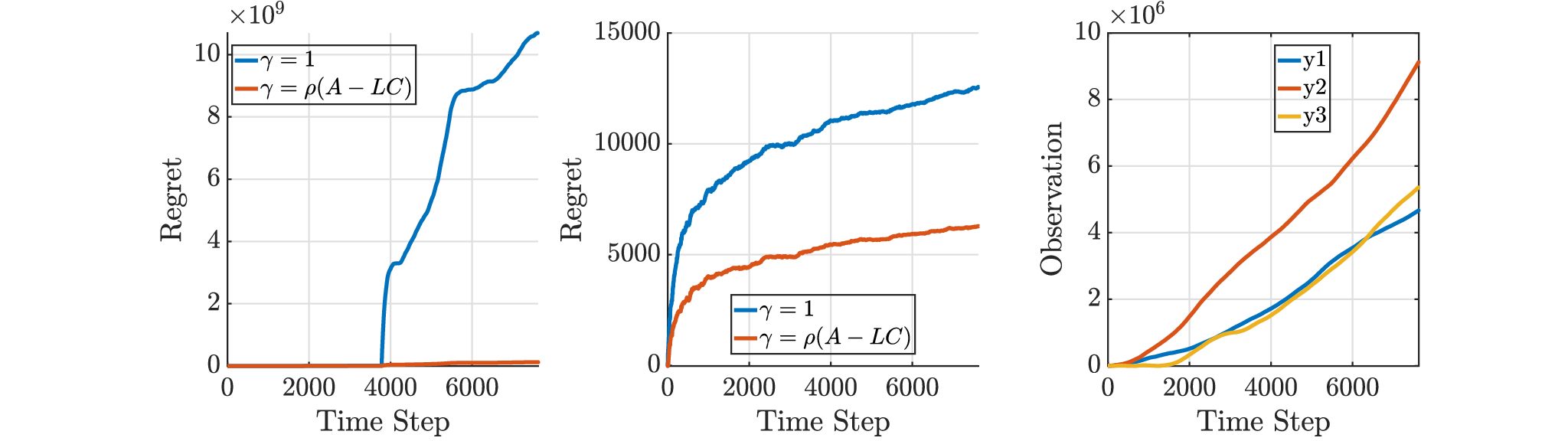
Refer to caption
Figure 5: Illustration figure for the problem of numerical stability

E.3 Discussion on the selection of β\beta

In Section C.2, we show that if the term β\beta is chosen as 2​κ+1log⁡(1/ρ⁡(A−L​C))\frac{2\kappa+1}{\log(1/\rho(A-LC))}, then the bias term C​(A−L​C)p​bk,pC(A-LC)^{p}b_{k,p} will be sufficiently small such that the error induced by bias will also be neglectable. Then the logarithmic regret of the online prediction Algorithm 1 can be guaranteed.

We find in numerical simulation that the bias error term ∑l=pkbl,p​Zl,p𝖳​V¯k,p−1​Zk+1,p−bk+1,p\sum_{l=p}^{k}b_{l,p}Z_{l,p}^{\mathsf{T}}\bar{V}_{k,p}^{-1}Z_{k+1,p}-b_{k+1,p} has an effect of cancellation. That is, even if the term bk+1,pb_{k+1,p} is large, the difference between bk+1,pb_{k+1,p} and ∑l=pkbl,p​Zl,p𝖳​V¯k,p−1​Zk+1,p\sum_{l=p}^{k}b_{l,p}Z_{l,p}^{\mathsf{T}}\bar{V}_{k,p}^{-1}Z_{k+1,p} is much smaller than that of bk+1,pb_{k+1,p}; see the Figure 6(a) for more details.

In Figure 6(a), the blue line represents the average of the bias term bk+1,pb_{k+1,p} over all kk in the last epoch with difference parameter β\beta. While the red line represents the average of canceled bias term ∑l=pkbl,p​Zl,p𝖳​V¯k,p−1​Zk+1,p−bk+1,p\sum_{l=p}^{k}b_{l,p}Z_{l,p}^{\mathsf{T}}\bar{V}_{k,p}^{-1}Z_{k+1,p}-b_{k+1,p} over kk with different β\beta. As we can see from Figure 6(a) that the canceled bias term is much smaller than the real bias term bk+1,pb_{k+1,p}. This phenomenon indicates that it is possible for us to choose a relatively smaller β\beta to reduce the length of the past horizon pp and balance a better trade-off between prediction error, effect of overfitting and computation cost.

Refer to caption
(a) Bias Cancellation
Refer to caption
(b) Traditional Forget
Figure 6: Supplementary experiments

E.4 Further experiments for theoretical verification

In this subsection, we provide numerical verification for our theoretical statements. In Fig. 6(b), we compare the upper bound of regression term ‖Ek,p​Z¯k,p​V¯k,p−12‖22\big\|E_{k,p}\bar{Z}_{k,p}\bar{V}_{k,p}^{-\frac{1}{2}}\big\|_{2}^{2} provided in [36, 12, 20] and in this paper.

In [36], it is shown that the regression term ‖Ek,p​Z¯k,p​V¯k,p−12‖22\big\|E_{k,p}\bar{Z}_{k,p}\bar{V}_{k,p}^{-\frac{1}{2}}\big\|_{2}^{2} is upper bounded by the determinant of V¯k,p\bar{V}_{k,p}, i.e.,

‖Ek,p​Z¯k,p​V¯k,p−12‖22≤O⁡(log⁡detV¯k,pδ​detλ​Dp−2)\big\|E_{k,p}\bar{Z}_{k,p}\bar{V}_{k,p}^{-\frac{1}{2}}\big\|_{2}^{2}\leq O\Big(\log\frac{\det\bar{V}_{k,p}}{\delta\det\lambda D_{p}^{-2}}\Big)

with high probability 1−δ1-\delta. However, in Appendix C, we managed to prove that the dominant term of ‖Ek,p​Z¯k,p​V¯k,p−12‖22\big\|E_{k,p}\bar{Z}_{k,p}\bar{V}_{k,p}^{-\frac{1}{2}}\big\|_{2}^{2} is around tr​(Z¯k,p​V¯k,p−1​Z¯k,p𝖳)\text{tr}\big(\bar{Z}_{k,p}\bar{V}_{k,p}^{-1}\bar{Z}_{k,p}^{\mathsf{T}}\big). In Figure 6(b), we compare the two different theoretical bounds with the real ‖Ek,p​Z¯k,p​V¯k,p−12‖22\big\|E_{k,p}\bar{Z}_{k,p}\bar{V}_{k,p}^{-\frac{1}{2}}\big\|_{2}^{2}, we select the value at k=2​Tl−2k=2T_{l}-2, i.e., the end of each epoch, for comparison. Then we can see that the determinant bound provided by [36, 12, 20] is, to some extent, conservative. The bound provided in this paper is sharper, but there is still some potential to be optimized.

Then we want to verify the theoretical result in Theorem 1. In Figure 7, we compare the regret with different orders of log⁡N\log N. The performance index is defined as

p⁡(i,N)=ℛNlogi⁡N,p(i,N)=\frac{\mathcal{R}_{N}}{\log^{i}N},

where the blue line denotes the performance of the online prediction algorithm proposed in [12] and the red line denotes the performance of Algorithm 1 proposed in this paper. It can be verified from this simulation that the regret of the online prediction algorithm appears to be O⁡(log2⁡N)O(\log^{2}N). The utilization of forgetting factor can improve the prediction performance, but cannot reduce the order of regret with log⁡N\log N.

Refer to caption
Figure 7: Illustration figure for the verification of theoretical regret bound.

Appendix F Further Discussions

F.1 Extension to systems with control input

In this subsection, we provide a summary on how to directly extend the theoretical results and techniques proposed in this paper to the case with control input, i.e., to predict the stochastic system

xk+1\displaystyle x_{k+1} =A​xk+B​uk+wk,wk∼𝒩⁡(0,Q)\displaystyle=Ax_{k}+Bu_{k}+w_{k},\hskip 9.24994ptw_{k}\sim\mathcal{N}(0,Q)
yk\displaystyle y_{k} =Cxk+Duk+vk,vk∼𝒩(0,R).\displaystyle=Cx_{k}+Du_{k}+v_{k},\hskip 9.24994ptv_{k}\sim\mathcal{N}(0,R).

With a similar technique in Section 2.2, we can obtain the regression model as

yk=Gp​Zk,p+D​uk+C⁡(A−L​C)​x^k−p+eky_{k}=G_{p}Z_{k,p}+Du_{k}+C(A-LC)\hat{x}_{k-p}+e_{k}

where GG and Zk,pZ_{k,p} are modified to be G=[Gp(1),Gp(2)]G=[G^{(1)}_{p},G^{(2)}_{p}], Zk,p=[Zk,p(1)​𝖳,Zk,p(2)​𝖳]𝖳Z_{k,p}=[Z_{k,p}^{(1)\mathsf{T}},Z_{k,p}^{(2)\mathsf{T}}]^{\mathsf{T}} where

Gp(1)\displaystyle G^{(1)}_{p} ≜[C​(A−L​C)p−1​L⋯C​L],\displaystyle\triangleq\begin{bmatrix}C(A-LC)^{p-1}L&\cdots&CL\end{bmatrix},
Gp(2)\displaystyle G^{(2)}_{p} ≜[C​(A−L​C)p−1​(B−L​D)⋯C⁡(B−L​D)],\displaystyle\triangleq\begin{bmatrix}C(A-LC)^{p-1}(B-LD)&\cdots&C(B-LD)\end{bmatrix},

and

Zk,p(1)=[yk−p𝖳,…,yk−1𝖳]𝖳,Zk,p(2)=[uk−p𝖳,…,uk−1𝖳]𝖳.Z^{(1)}_{k,p}=\begin{bmatrix}y_{k-p}^{\mathsf{T}},\dots,y_{k-1}^{\mathsf{T}}\end{bmatrix}^{\mathsf{T}},\hskip 9.24994ptZ^{(2)}_{k,p}=\begin{bmatrix}u_{k-p}^{\mathsf{T}},\dots,u_{k-1}^{\mathsf{T}}\end{bmatrix}^{\mathsf{T}}.

The forgetting process can be modified as

Z~k,p=[Dp(1)Dp(2)]​[Zk,p(1)Zk,p(2)],\tilde{Z}_{k,p}=\begin{bmatrix}D_{p}^{(1)}&\\ &D_{p}^{(2)}\end{bmatrix}\begin{bmatrix}Z_{k,p}^{(1)}\\ Z_{k,p}^{(2)}\end{bmatrix},

where Dp(1)D_{p}^{(1)} and Dp(2)D_{p}^{(2)} are diagonal matrices with proper dimension. Then for uniformly bounded input uku_{k}, we can verify that our algorithm directly guarantees a logarithmic regret ℛN\mathcal{R}_{N} to the optimal predictor. The regression process can directly follow the steps in Algorithm 1.

F.2 Matrix forgetting factor

For technical improvement, we can also consider applying the matrix-based forgetting factor to balance the regression model, i.e.,

Dp=diag⁡(Γp−1,Γp−2,…,Γ,I),D_{p}=\operatorname{diag}(\Gamma^{p-1},\Gamma^{p-2},\dots,\Gamma,I),

and the corresponding balanced model takes the form as

G~p≜[C​(A−L​C)p−1​L​Γ−(p−1),⋯,C​L],\displaystyle\tilde{G}_{p}\triangleq\begin{bmatrix}C(A-LC)^{p-1}L\Gamma^{-(p-1)},\cdots,CL\end{bmatrix},

where the forgetting matrix Γ\Gamma can be designed with some system identification based techniques [8, 13, 14]. Developing the prediction technique by potentially bridging the direct and indirect methods together to improve performance might be possible.