跳到论文正文
W Papers独立论文阅读器 arXiv:2505.08970 论文正文 计算阅读时间 · 0%
引用这篇论文根据当前论文元数据生成,正式投稿前建议核对。


License: arXiv.org perpetual non-exclusive license
arXiv:2505.08970v2 [math.NA] 28 Jun 2026

Approximation of viscous transport and conservative equations with one sided Lipschitz velocity fieldsThanks: Submitted to the editors DATE.

Fabio Camilli ††thanks: Dip. di Ingegneria e Geologia, Univ. “G. D’Annunzio” Chieti-Pescara, viale Pindaro 42, 65127 Pescara (Italy), (). Email: fabio.camilli@unich.it    Adriano Festa ††thanks: Dip. di Scienze Matematiche “G. L. Lagrange”, Politecnico di Torino, Corso Duca degli Abruzzi 24, 10129 Torino (Italy), (). Email: adriano.festa@polito.it    Luciano Marzufero ††thanks: Facoltà di Economia e Management, Libera Università di Bolzano, piazza Università 1, 39100 Bolzano (Italy)    () Email: luciano.marzufero@unibz.it
Abstract

The aim of this work is to investigate semi-Lagrangian approximation schemes on unstructured grids for viscous transport and conservative equations with measurable coefficients that satisfy a one-sided Lipschitz condition. To establish the convergence of the schemes, we exploit the characterization of the solution for these equations expressed in terms of measurable time-dependent viscosity solution and, respectively, duality solution. We supplement our theoretical analysis with various numerical examples to illustrate the features of the schemes.

keywords
one-sided Lipschitz condition, viscous transport equation, measure-valued solution, semi-Lagrangian schemes.
Funding.
This work was partially supported by by INdAM-GNAMPA, PRIN PNRR P20225SP98 “Some mathematical approaches to climate change and its impacts”, “INdAM–GNCS Project”, codice CUPE53C24001950001.
MSC
35K20, 35D30, 49L25, 65M12.

1 Introduction

We investigate semi-Lagrangian approximation schemes for the viscous transport equation

−∂u∂t−tr⁡[a⁡(t,x)​D2​u]+b⁡(t,x)⋅D​u=0in ​(0,T)×ℝd,with ​u​(T,⋅)=uT,-\frac{\partial u}{\partial t}-\operatorname{tr}[a(t,x)D^{2}u]+b(t,x)\cdot Du=0\quad\text{in }(0,T)\times\mathbb{R}^{d},\quad\text{with }u(T,\cdot)=u_{T}, (1.1)

and the viscous conservative equation

∂f∂t−D2⋅[a⁡(t,x)​f]−div⁡(b⁡(t,x)​f)=0in ​(0,T)×ℝd,with ​f​(0,⋅)=f0.\frac{\partial f}{\partial t}-D^{2}\cdot[a(t,x)f]-\diver(b(t,x)f)=0\quad\text{in }(0,T)\times\mathbb{R}^{d},\quad\text{with }f(0,\cdot)=f_{0}. (1.2)

The well-posedness of these problems has been extensively studied in the literature. For the first-order case where a⁡(x)≡0a(x)\equiv 0, relevant results can be found in [1, 15]. The second-order case has been investigated in [21, 17], and a more comprehensive list of references is available in [23]. These works generally assume that the divergence of bb is absolutely continuous with respect to the Lebesgue measure.

In this work, we consider b:[0,T]×ℝd⟶ℝdb:[0,T]\times\mathbb{R}^{d}\longrightarrow\mathbb{R}^{d} as a measurable function satisfying the one-sided Lipschitz condition ((OSLC) in short)

(b(t,x)−b(t,y))⋅(x−y)≥−C(t)|x−y|2,∀t∈[0,T],x,y∈ℝd,(b(t,x)-b(t,y))\cdot(x-y)\geq-C(t)|x-y|^{2},\quad\forall t\in[0,T],\,x,y\in\mathbb{R}^{d}, (1.3)

for some C∈L1​(0,T)C\in L^{1}(0,T) with C≥0C\geq 0. Additionally, aa is assumed to be a regular, degenerate matrix. Since the (OSLC) framework does not rule out the possibility that the measure div⁡b\diver b may include a singular component, this limitation prevents the application of the aforementioned theories to the present situation.

For the first-order case satisfying the (OSLC) condition, the problems (1.1) and (1.2) have been addressed for example in [5, 6, 10, 26] (see Remark 2.9 concerning the sign of bb). In [23], a general theory has been recently developed both in the first order case and in the second order one. In this latter work, various characterizations of the “good” solutions, i.e. solutions obtained as limits of equations with regular approximations of bb, are provided. Specifically, the “good” solutions are characterized as measurable time-dependent viscosity solutions for the transport equation, and duality solutions for the conservative equation.

Regarding the approximation of these equations in the regular case, a vast body of literature exists due to their relevance in diverse fields such as fluid dynamics, financial mathematics, optimal transport, and Mean-Field Games. For first-order equations satisfying the (OSLC) condition, we refer to [13, 14, 20, 7]. The second-order case in the Di Perna-Lions setting has been recently studied in [25], whereas, to the best of our knowledge, no articles have addressed the (OSLC) case.

Here, we examine semi-Lagrangian approximation schemes for (1.1) and (1.2) under the (OSLC) condition. For an introduction to semi-Lagrangian scheme for the first-order case, we refer to [16], while the second-order case has been studied, for instance, in [4, 8, 11, 12]. Semi-Lagrangian methods offer a distinct advantage over traditional approaches like finite differences and finite volumes. Instead of directly approximating the partial differential equations themselves, they focus on approximating the underlying dynamics. This allows to employ the assumption (OSLC) to derive properties of the discrete trajectories, which subsequently inform the approximation scheme. These properties enable us to establish the convergence of the semi-Lagrangian approximation scheme for the viscous transport equation by exploiting the characterization of the solution as time-measurable viscosity solution. The proof utilizes a classical stability result by Barles and Souganidis [3], adapted to this specific context.

For the conservation equation, we adopt the scheme proposed in [11, 12], which is designed to handle linear and nonlinear Fokker-Planck equations with continuous coefficients on structured grids. For linear equations, our work generalizes their results to encompass cases involving irregular coefficients and general unstructured grids. Moreover, we precisely characterize the scheme’s limit as a duality solution of (1.2). These generalizations present new challenges, particularly in establishing the regularity properties of the discrete solution, which are critical for achieving convergence in the limit. At the discrete level, we derive a duality formula analogous to the one in the continuous setting and, exploiting this formula and the convergence result for (1.1), we prove that the scheme converges to the duality solution of (1.2) in the sense of weak convergence of measures.
While the results presented in this paper apply to the first-order problem, it is important to note that, in this case, error estimates for a finite difference scheme are derived in terms of the L∞​([0,T],L1​(ℝd))L^{\infty}([0,T],L^{1}(\mathbb{R}^{d})) norm for the transport equation (see [13]) and the pp-Wasserstein distance for conservative equation (see [14]).
In the numerical section, we show in practice the performances of the numerical techniques proposed here. We consider an example in a one-dimensional case, where it is possible to compare the approximation with the analytical solution of the problem and two examples in the two dimensional case, the first one with a continuous vector field, and the second one with a discontinuous vector field verifying the (OSLC) condition.

Notations

Let Cb​(ℝd)C_{b}(\mathbb{R}^{d}) represents the set of bounded continuous functions and C0,1​(ℝd)C^{0,1}(\mathbb{R}^{d}) the set of the Lipschitz continuous function in ℝd\mathbb{R}^{d}. We denote by ℳ⁡(ℝd)\mathcal{M}(\mathbb{R}^{d}) the space of non-negative measures on ℝd\mathbb{R}^{d}, defined with respect to the Borel σ\sigma-algebra ℬ⁡(ℝd)\mathcal{B}(\mathbb{R}^{d}). This space is equipped with the weak topology σ⁡(ℳ⁡(ℝd),Cb​(ℝd))\sigma(\mathcal{M}(\mathbb{R}^{d}),C_{b}(\mathbb{R}^{d})). Next, we consider the space C⁡([0,T],ℳ⁡(ℝd))C([0,T];\mathcal{M}(\mathbb{R}^{d})), which represents flows of measures. This space is endowed with the topology of uniform convergence over [0,T][0,T].
Let 𝒫⁡(ℝd)\mathcal{P}(\mathbb{R}^{d}) be the subset of ℳ⁡(ℝd){\mathcal{M}}(\mathbb{R}^{d}) consisting of probability measures defined on (ℝd,ℬ⁡(ℝd))(\mathbb{R}^{d},\mathcal{B}(\mathbb{R}^{d})). Furthermore, we define 𝒫p​(ℝd)\mathcal{P}_{p}(\mathbb{R}^{d}) as the space of probability measures that have a finite pp-th order moment for p≥1p\geq 1, given by:

𝒫p​(ℝd)={μ∈𝒫⁡(ℝd):∫ℝd|x|p​μ​(𝑑x)<∞}.\mathcal{P}_{p}(\mathbb{R}^{d})=\left\{\mu\in\mathcal{P}(\mathbb{R}^{d}):\int_{\mathbb{R}^{d}}|x|^{p}\,\mu(dx)<\infty\right\}.

This space is equipped with the standard Wasserstein distance 𝒲p\mathcal{W}_{p} (see [28]). For p=1p=1, by the Kantorovich–Rubinstein duality formula, we have for μ,μ′∈𝒫1​(ℝd)\mu,\mu^{\prime}\in\mathcal{P}_{1}(\mathbb{R}^{d})

𝒲1(μ,μ′)=sup{∫ℝdϕ(x)d(μ−μ′):ϕ:ℝd⟶ℝis 1-Lipschitz continuous }.\mathcal{W}_{1}(\mu,\mu^{\prime})=\sup\left\{\int_{\mathbb{R}^{d}}\phi(x)d(\mu-\mu^{\prime}):\,\phi:\mathbb{R}^{d}\longrightarrow\mathbb{R}\,\mbox{is $1$-Lipschitz continuous }\right\}.

For a locally bounded function g:ℝd→ℝg:\mathbb{R}^{d}\to\mathbb{R}, we define

lim infz→xg∗(z)=limr→0inf{g(z):z∈B(0,r)},\displaystyle\liminf_{z\to x}\hskip-2.0pt{}_{*}\,g(z)=\lim_{r\to 0}\,\inf\{g(z):\,z\in B(0,r)\},
lim supz→x∗g⁡(z)=limr→0sup{g⁡(z):z∈B⁡(0,r)}.\displaystyle\limsup_{z\to x}\hskip-2.0pt^{*}\,g(z)=\lim_{r\to 0}\,\sup\{g(z):\,z\in B(0,r)\}.

2 The model problem

The results of this section are taken from [23], whose notation we will adhere to. We assume that b:[0,T]×ℝd⟶ℝdb:[0,T]\times\mathbb{R}^{d}\longrightarrow\mathbb{R}^{d} is a measurable function satisfying: for all t∈[0,T]t\in[0,T] and x,y∈ℝdx,y\in\mathbb{R}^{d},

supx∈ℝd|b⁡(t,x)|1+|x|≤C0​(t),(b⁡(t,x)−b⁡(t,y))⋅(x−y)≥−C1​(t)​|x−y|2,\begin{split}&\quad\sup_{x\in\mathbb{R}^{d}}\frac{|b(t,x)|}{1+|x|}\leq C_{0}(t),\\[4.0pt] &\quad(b(t,x)-b(t,y))\cdot(x-y)\geq-C_{1}(t)|x-y|^{2},\end{split} (2.1)

for some non negative functions C0,C1∈L1​(0,T)C_{0},C_{1}\in L^{1}(0,T). Moreover a=12​σ​σTa=\frac{1}{2}\sigma\sigma^{T} for σ:[0,T]×ℝd⟶ℝd×r\sigma:[0,T]\times\mathbb{R}^{d}\longrightarrow\mathbb{R}^{d\times r} satisfying

supx∈ℝd|σ⁡(t,x)|1+|x|+supy,z∈ℝd|σ⁡(t,y)−σ⁡(t,z)||y−z|≤C2​(t)\sup_{x\in\mathbb{R}^{d}}\frac{|\sigma(t,x)|}{1+|x|}+\sup_{y,z\in\mathbb{R}^{d}}\frac{|\sigma(t,y)-\sigma(t,z)|}{|y-z|}\leq C_{2}(t) (2.2)

for a non negative function C2∈L2​(0,T)C_{2}\in L^{2}(0,T). We consider the SDE

{ds​Φs,t​(x)=−b⁡(s,Φs,t​(x))​d​s+σ⁡(s,Φs,t​(x))​d​Wss∈[t,T],Φt,t​(x)=x∈ℝd,\begin{cases}d_{s}\Phi_{s,t}(x)=-b(s,\Phi_{s,t}(x))ds+\sigma(s,\Phi_{s,t}(x))dW_{s}&s\in[t,T],\\ \Phi_{t,t}(x)=x\in\mathbb{R}^{d},\end{cases} (2.3)

where W:Ω×[0,T]⟶ℝrW:\Omega\times[0,T]\longrightarrow\mathbb{R}^{r} is a standard Brownian motion on a given probability space (Ω,ℱ,ℙ)(\Omega,\mathcal{F},\mathbb{P}).

Proposition 2.1.

For every (t,x)∈[0,T]×ℝd(t,x)\in[0,T]\times\mathbb{R}^{d} and ℙ\mathbb{P}-almost surely, there exists a unique strong solution Φs,t​(x)\Phi_{s,t}(x) of (2.3) defined on [t,T]×ℝd[t,T]\times\mathbb{R}^{d}. For all p∈[2,∞)p\in[2,\infty), there exists a constant C=Cp>0C=C_{p}>0 depending only on the assumptions (2.1) and (2.2) such that

𝔼​|Φs,t​(x)−Φs,t​(y)|p≤C​|x−y|pfor all ​0≤t≤s≤T​ and ​x,y∈ℝd,\mathbb{E}|\Phi_{s,t}(x)-\Phi_{s,t}(y)|^{p}\leq C|x-y|^{p}\quad\text{for all }0\leq t\leq s\leq T\text{ and }x,y\in\mathbb{R}^{d}, (2.4)
𝔼​|Φs,t​(x)|p≤C⁡(|x|p+1)for all ​0≤t≤s≤T​ and ​x∈ℝd,\mathbb{E}|\Phi_{s,t}(x)|^{p}\leq C(|x|^{p}+1)\quad\text{for all }0\leq t\leq s\leq T\text{ and }x\in\mathbb{R}^{d}, (2.5)

and

𝔼​|Φs1,t​(x)−Φs2,t​(x)|p≤C⁡(1+|x|)​|s1−s2|p/2\mathbb{E}|\Phi_{s_{1},t}(x)-\Phi_{s_{2},t}(x)|^{p}\leq C(1+|x|)|s_{1}-s_{2}|^{p/2}

for all t∈[0,T]t\in[0,T], s1,s2∈[t,T]s_{1},s_{2}\in[t,T], and x∈ℝdx\in\mathbb{R}^{d}. Moreover, for all 0≤r≤s≤t≤T0\leq r\leq s\leq t\leq T, we have Φt,s∘Φs,r=Φt,r\Phi_{t,s}\circ\Phi_{s,r}=\Phi_{t,r} with probability one.

If (bε)ε>0(b^{\varepsilon})_{\varepsilon>0} is a regularization of bb satisfying

{(bε)ε>0⊂L1([0,T],C0,1(ℝd)),limε→0bε=b a.e. in [0,T]×ℝd, andbε​ satisfies (2.1) uniformly in ε>0,\left\{\begin{split}&(b^{\varepsilon})_{\varepsilon>0}\subset L^{1}([0,T],C^{0,1}(\mathbb{R}^{d})),\quad\lim_{\varepsilon\to 0}b^{\varepsilon}=b\text{ a.e. in }[0,T]\times\mathbb{R}^{d},\text{ and}\\ &b^{\varepsilon}\text{ satisfies \eqref{hyp:OSLC} uniformly in $\varepsilon>0$},\end{split}\right. (2.6)

then the corresponding stochastic flows Φε\Phi^{\varepsilon} converge locally uniformly to Φ\Phi as ε→0\varepsilon\to 0 with probability one.

2.1 The viscous transport equation

Theorem 2.2.

Let uT∈C⁡(ℝd)u_{T}\in C(\mathbb{R}^{d}) and define u:[0,T]×ℝd⟶ℝu:[0,T]\times\mathbb{R}^{d}\longrightarrow\mathbb{R} by

u⁡(t,x)=𝔼⁡[uT​(ΦT,t​(x))].u(t,x)=\mathbb{E}[u_{T}(\Phi_{T,t}(x))]. (2.7)

If (bε)ε>0(b^{\varepsilon})_{\varepsilon>0} satisfy (2.6) and uεu^{\varepsilon} is the solution of (1.1) with velocity bεb^{\varepsilon}, then, as ε→0\varepsilon\to 0, uεu^{\varepsilon} converges locally uniformly to uu. Moreover, if uT∈C0,1​(ℝd)u_{T}\in C^{0,1}(\mathbb{R}^{d}), then

sup(t,x,y)∈[0,T]×ℝd×ℝd|u⁡(t,x)−u⁡(t,y)||x−y|+sup(r,s,x)∈[0,T]×ℝd|u⁡(r,x)−u⁡(s,x)||r−s|1/2​(1+|x|)<∞,\sup_{(t,x,y)\in[0,T]\times\mathbb{R}^{d}\times\mathbb{R}^{d}}\frac{|u(t,x)-u(t,y)|}{|x-y|}+\sup_{(r,s,x)\in[0,T]\times\mathbb{R}^{d}}\frac{|u(r,x)-u(s,x)|}{|r-s|^{1/2}(1+|x|)}<\infty,

and uu is a distributional solution of (1.1).

Although (2.7) represents a distributional solution that arises uniquely through the regularization of bb, distributional solutions are generally not unique. In [23], it is proved that the function uu given by (2.7) can be uniquely identified as the solution of (1.1) in time measurable viscosity sense. We define, for (t,x,p)∈[0,T]×ℝd×ℝd(t,x,p)\in[0,T]\times\mathbb{R}^{d}\times\mathbb{R}^{d},

b¯(t,x,p)=lim infz→xb∗(t,z)⋅pandb¯(t,x,p)=lim supz→x∗b(t,z)⋅p.\underline{b}(t,x,p)=\liminf_{z\to x}\hskip-2.0pt{}_{*}b(t,z)\cdot p\quad\text{and}\quad\overline{b}(t,x,p)=\limsup_{z\to x}\hskip-2.0pt^{*}b(t,z)\cdot p. (2.8)

For fixed (t,x)∈[0,T]×ℝd(t,x)\in[0,T]\times\mathbb{R}^{d}, b¯(t,x,⋅)\underline{b}(t,x,\cdot) and b¯(t,x,⋅)\overline{b}(t,x,\cdot) are Lipschitz continuous on ℝd\mathbb{R}^{d}, and, for fixed (t,p)∈[0,T](t,p)\in[0,T], b¯​(t,⋅,p)\underline{b}(t,\cdot,p) and b¯​(t,⋅,p)\overline{b}(t,\cdot,p) are respectively lower semicontinous (l.s.c.) and upper semicontinuous (u.s.c.).

Definition 2.3.

An u.s.c. (resp., l.s.c.) function uu is called a viscosity subsolution (resp. supersolution) of (1.1) if u⁡(⋅,T)≤uTu(\cdot,T)\leq u_{T} (resp., ≥\geq) and for all ψ∈C2​(ℝd)\psi\in C^{2}(\mathbb{R}^{d})

−dd​t​maxx∈ℝd​{u⁡(t,x)−ψ⁡(x)}≤inf{tr⁡[a⁡(t,y)​D2​ψ​(y)]−b¯​(t,y,D​ψ​(y)):y∈arg⁡max⁡{u⁡(t,⋅)−ψ⁡(⋅)}}-\frac{d}{dt}\max_{x\in\mathbb{R}^{d}}\left\{u(t,x)-\psi(x)\right\}\\ \leq\inf\left\{\operatorname{tr}[a(t,y)D^{2}\psi(y)]-\underline{b}(t,y,D\psi(y)):y\in\arg\max\{u(t,\cdot)-\psi(\cdot)\}\right\}
(resp.−dd​tminx∈ℝd{u(t,x)−ψ(x)}OPEN≥sup{tr⁡[a⁡(t,y)​D2​ψ​(y)]−b¯​(t,y,D​ψ​(y)):y∈arg⁡min⁡{u⁡(t,⋅)−ψ⁡(⋅)}})\Big(resp.\quad-\frac{d}{dt}\min_{x\in\mathbb{R}^{d}}\left\{u(t,x)-\psi(x)\right\}\\ \geq\sup\left\{\operatorname{tr}[a(t,y)D^{2}\psi(y)]-\overline{b}(t,y,D\psi(y)):y\in\arg\min\{u(t,\cdot)-\psi(\cdot)\}\right\}\Big)

in distributional sense. If u∈C⁡([0,T]×ℝd)u\in C([0,T]\times\mathbb{R}^{d}) is both a subsolution and supersolution, we say that uu is a viscosity solution.

We have the following Comparison Principle:

Theorem 2.4.

If uu and vv are respectively a sub and supersolution of (1.1) such that

sup(t,x)∈[0,T]×ℝdu⁡(t,x)1+|x|+sup(s,y)∈[0,T]×ℝd−v⁡(s,y)1+|y|<∞,\sup_{(t,x)\in[0,T]\times\mathbb{R}^{d}}\frac{u(t,x)}{1+|x|}+\sup_{(s,y)\in[0,T]\times\mathbb{R}^{d}}\frac{-v(s,y)}{1+|y|}<\infty,

then t↦supx∈ℝd{u⁡(t,x)−v⁡(t,x)}t\mapsto\sup_{x\in\mathbb{R}^{d}}\left\{u(t,x)-v(t,x)\right\} is nondecreasing.

As a consequence of the previous result, the “good” distributional solution of (1.1) can be uniquely characterized.

Corollary 2.5.

Assume uT∈C⁡(ℝd)u_{T}\in C(\mathbb{R}^{d}) is uniformly continuous and uT⋅(1+|x|)−1∈L∞​(ℝd)u_{T}\cdot(1+|x|)^{-1}\in L^{\infty}(\mathbb{R}^{d}). Then (2.7) is the unique viscosity solution of (1.1).

Remark 2.6.

As noted in [23, Subsection 3.1.3], there generally exist distributional solutions to (1.1) that are not viscosity solutions to the problem. The uniqueness of distributional solutions can be ensured by requiring that b∈C⁡([0,T]×ℝd)b\in C([0,T]\times\mathbb{R}^{d}) satisfies the (OSLC) condition in (2.1) and that uT∈C0,1​(ℝd)u_{T}\in C^{0,1}(\mathbb{R}^{d}).

2.2 The conservative equation

For the conservative equation (1.2), the tendency of the backward flow to concentrate on sets of zero Lebesgue measure suggests that, even if f0f_{0} is absolutely continuous with respect to the Lebesgue measure, the solution f⁡(t,⋅)f(t,\cdot) may develop a singular component for tt positive. Hence, it is natural the introduce a notion of solution in the sense of measure.

Definition 2.7.

A map f∈C⁡([0,T],ℳ)f\in C([0,T],\mathcal{M}) is called a solution of (1.2) if, for all t∈[0,T]t\in[0,T] and g∈Cb​(ℝd)g\in C_{b}(\mathbb{R}^{d}),

∫ℝdg⁡(x)​f​(t,𝑑x)=∫ℝd𝔼⁡[g⁡(Φt,0​(x))]​f0​(𝑑x),\int_{\mathbb{R}^{d}}g(x)f(t,dx)=\int_{\mathbb{R}^{d}}\mathbb{E}[g(\Phi_{t,0}(x))]f_{0}(dx),

where Φt,0\Phi_{t,0} is the stochastic flow satisfying (2.3).

Solutions as in the previous definition are called duality solutions because 𝔼​[g​(Φt,0​(x))]\mathbb{E}[g(\Phi_{t,0}(x))] is the solution of (1.1) with terminal value gg at time tt (cfr. [9]). If f0f_{0} is a probability measure, then f⁡(t,⋅)f(t,\cdot) is the law of the stochastic process Φt,0​(X0)\Phi_{t,0}(X_{0}), where X0X_{0} is a random variable with law f0f_{0}.

Theorem 2.8.

Assume that f0∈ℳf_{0}\in\mathcal{M}. Then, there exists a unique duality solution ff of (1.2). If, for ε>0\varepsilon>0, fεf^{\varepsilon} is the solution corresponding to bεb^{\varepsilon} as in (2.6), then, as ε→0\varepsilon\to 0, fεf^{\varepsilon} converges weakly in the sense of measures to ff. If 1≤p≤∞1\leq p\leq\infty, f0,g0∈𝒫pf_{0},g_{0}\in\mathcal{P}_{p}, and ff and gg are the corresponding duality solutions, then, for some C>0C>0 depending on pp and the constants in (2.1), 𝒲p​(f⁡(t),g⁡(t))≤C​𝒲p​(f0,g0)\mathcal{W}_{p}(f(t),g(t))\leq C\mathcal{W}_{p}(f_{0},g_{0}).

Remark 2.9.

Note that, in the conservative first-order case, the results presented in this section apply to the equation

∂f∂t+div⁡(−b⁡(t,x)​f)=0in ​(0,T)×ℝd,with ​f​(0,⋅)=f0.\frac{\partial f}{\partial t}+\diver(-b(t,x)f)=0\quad\text{in }(0,T)\times\mathbb{R}^{d},\quad\text{with }f(0,\cdot)=f_{0}. (2.9)

therefore, consistently with the corresponding second-order problem (1.2) which requires the use of the forward flow defined by (2.3), the velocity field, also in this first-order case is −b-b. This notation choice has been made to keep all the study consistent with [23].

3 The numerical scheme

In this section, we consider semi-Lagrangian schemes for (1.1) and (1.2) defined on an unstructured mesh. Given N∈ℕN\in{\mathbb{N}} we set h:=T/Nh:=T/N and tk:=k​ht_{k}:=kh for k=0,…,Nk=0,\ldots,N. Moreover, given Δ​x>0{\Delta x}>0, we consider a triangular mesh 𝒯Δ​x=(Tτ)τ∈𝒦Δ​x\mathcal{T}^{\Delta x}=(T_{\tau})_{\tau\in\mathcal{K}^{\Delta x}} such that ⋃τ∈𝒦Δ​xTτ=ℝd\bigcup_{\tau\in\mathcal{K}^{\Delta x}}T_{\tau}=\mathbb{R}^{d}, Tτ∩Tλ=∅T_{\tau}\cap T_{\lambda}=\emptyset if τ≠λ\tau\neq\lambda. We assume that supτ[diam​(Tτ)]≤Δ​x\sup_{\tau}[\text{diam}(T_{\tau})]\leq{\Delta x} and infτ[height​(Tτ)]>0\inf_{\tau}[\text{height}(T_{\tau})]>0. We set Δ=(h,Δ​x)\Delta=(h,{\Delta x}).
Given the set of the vertices of the triangulation 𝒱Δ​x={xi}i∈ℐΔ​x\mathcal{V}^{\Delta x}=\{x_{i}\}_{i\in\mathcal{I}^{\Delta x}}, we consider a ℚ1\mathbb{Q}_{1} basis (βi)i∈ℐΔ​x(\beta_{i})_{i\in\mathcal{I}^{\Delta x}}, where βi:ℝd→ℝ\beta_{i}:\mathbb{R}^{d}\to\mathbb{R} is a polynomial of degree less than or equal to 11 and satisfies βi​(xj)=1\beta_{i}(x_{j})=1 if i=ji=j and βi​(xj)=0\beta_{i}(x_{j})=0, otherwise. Moreover, the support supp​(βi)\mbox{supp}(\beta_{i}) of βi\beta_{i} is compact and

0≤βi≤1∀i∈ℐΔ​x,∑i∈ℐΔ​xβi​(x)=1​∀x∈ℝd.0\leq\beta_{i}\leq 1\quad\forall\;i\in\mathcal{I}^{\Delta x},\qquad\sum_{i\in\mathcal{I}^{\Delta x}}\beta_{i}(x)=1\hskip 8.5359pt\forall\;x\in\mathbb{R}^{d}. (3.1)

Let B⁡(𝒱Δ​x)B(\mathcal{V}^{\Delta x}) be the space of bounded functions on 𝒱Δ​x\mathcal{V}^{\Delta x} and, for ϕ∈B⁡(𝒱Δ​x)\phi\in B(\mathcal{V}^{\Delta x}), let ϕ⁡(i)\phi(i) be its value at xix_{i}. We consider the following linear interpolation operator

I⁡[ϕ]​(⋅):=∑i∈ℐΔ​xβi​(⋅)​ϕ​(i)for ​ϕ∈B⁡(𝒱Δ​x).I[\phi](\cdot):=\sum_{i\in\mathcal{I}^{{\Delta x}}}\beta_{i}(\cdot)\,\phi(i)\qquad\mbox{for }\phi\in B(\mathcal{V}^{\Delta x}).

Given ϕ∈Cb​(ℝd)\phi\in C_{b}(\mathbb{R}^{d}), let us define ϕ^∈B⁡(𝒱Δ​x)\hat{\phi}\in B(\mathcal{V}^{\Delta x}) by ϕ^​(i):=ϕ​(xi)\hat{\phi}(i):=\phi(x_{i}) for all i∈ℐΔ​xi\in\mathcal{I}^{\Delta x}. If ϕ:ℝd⟶ℝ\phi:\mathbb{R}^{d}\longrightarrow\mathbb{R} is Lipschitz with constant LL, then

supx∈ℝd|I⁡[ϕ^]​(x)−ϕ⁡(x)|≤L​Δ​x.\sup_{x\in\mathbb{R}^{d}}|I[\hat{\phi}](x)-\phi(x)|\leq L{\Delta x}. (3.2)

Moreover, if ϕ∈C2​(ℝd)\phi\in C^{2}(\mathbb{R}^{d}) with bounded second order derivatives, then

supx∈ℝd|I⁡[ϕ^]​(x)−ϕ⁡(x)|≤C​Δ​x2\sup_{x\in\mathbb{R}^{d}}|I[\hat{\phi}](x)-\phi(x)|\leq C{\Delta x}^{2} (3.3)

with CC independent of Δ​x{\Delta x}.
We consider a standard mollifier ρ∈C∞​(ℝd)\rho\in C^{\infty}(\mathbb{R}^{d}), ρ≥0\rho\geq 0, supp⁡(ρ)⊂B⁡(0,1)\supp(\rho)\subset B(0,1), and ∫ℝdρ​𝑑x=1\int_{\mathbb{R}^{d}}\rho dx=1 and we set ρh=h−dρ(⋅/h)\rho_{h}=h^{-d}\rho(\cdot/h) where hh is the time step. We define

bhk​(x)=1h​∫tktk+1bh​(s,x)​dswherebh​(s,x)=(b⁡(s,⋅)∗ρh)​(x),σkh,ℓ(x)=1h∫tktk+1σℓ(s,x)ds,ℓ=1,…,r.\begin{split}&b^{k}_{h}(x)=\frac{1}{h}\int_{t_{k}}^{t_{k+1}}b_{h}(s,x)ds\quad\text{where}\quad b_{h}(s,x)=(b(s,\cdot)*\rho_{h})(x),\\ &\sigma^{k}_{h,\ell}(x)=\frac{1}{h}\int_{t_{k}}^{t_{k+1}}\sigma_{\ell}(s,x)ds,\quad\ell=1,\dots,r.\end{split} (3.4)

We approximate the stochastic flow (2.3) by a discrete-time and countably-state space Markov chain {Φk,mΔ​(xs);k=m,…,N}\{\Phi^{\Delta}_{k,m}(x_{s})\;;\;k=m,\ldots,N\} with state space 𝒱Δ​x\mathcal{V}^{\Delta x} and transition probabilities

pj​ik:=ℙ⁡(Φk+1,mΔ​(xs)=xi|Φk,mΔ​(xs)=xj)=12​r​∑ℓ=1r[βi​(𝒳ℓ,+k​(xj))+βi​(𝒳ℓ,−k​(xj))],∀i,j∈ℐΔ​x,ℙ⁡(Φm,mΔ​(xs)=xj)=δs,j,\begin{split}&p_{ji}^{k}:=\mathbb{P}\left(\Phi^{\Delta}_{k+1,m}(x_{s})=x_{i}\;\big|\;\Phi^{\Delta}_{k,m}(x_{s})=x_{j}\right)\\ &\qquad=\frac{1}{2r}\sum\limits_{\ell=1}^{r}\left[\beta_{i}(\mathcal{X}^{k}_{\ell,+}(x_{j}))+\beta_{i}(\mathcal{X}^{k}_{\ell,-}(x_{j}))\right],\quad\;\forall\;i,j\in\mathcal{I}^{\Delta x},\\ &\mathbb{P}\left(\Phi^{\Delta}_{m,m}(x_{s})=x_{j}\right)=\delta_{s,j},\end{split} (3.5)

where, for x∈ℝdx\in\mathbb{R}^{d}, k=0,…,N−1k=0,\ldots,N-1 and ℓ=1,…,r\ell=1,\ldots,r

𝒳ℓ,+k​(x):⁣=x−h​bhk​(x)+r​h​σh,ℓk​(x),𝒳ℓ,−k​(x):⁣=x−h​bhk​(x)−r​h​σh,ℓk​(x).\begin{array}[]{rcl}\mathcal{X}^{k}_{\ell,+}(x)&:=&x-hb_{h}^{k}(x)+\sqrt{rh}\sigma^{k}_{h,\ell}(x),\\[4.0pt] \mathcal{X}^{k}_{\ell,-}(x)&:=&x-hb_{h}^{k}(x)-\sqrt{rh}\sigma^{k}_{h,\ell}(x).\end{array} (3.6)
Remark 3.1.

The previous approximation is motivated by the following construction. Given the equation (2.3), we approximate

Φt+h,t​(x)=Φt,t​(x)−∫tt+hb⁡(s,Φs,t​(x))​𝑑s+∫tt+hσ⁡(s,Φs,t​(x))​d​Ws\Phi_{t+h,t}(x)=\Phi_{t,t}(x)-\int_{t}^{t+h}b(s,\Phi_{s,t}(x))ds+\int_{t}^{t+h}\sigma(s,\Phi_{s,t}(x))dW_{s}

by the rr-dimensional random walk with NN time steps

Φ~tk+1,tkh​(xi)=Φ~tk,tkh​(xi)−h​∫tktk+1b⁡(s,Φ~tk,tkh​(xi))​𝑑s+r​h​∫tktk+1σ⁡(s,Φ~tk,tkh​(xi))​Z​𝑑s=xi−h​bhk​(xi)+r​h​σhk​(xi)​Z,\begin{split}\tilde{\Phi}^{h}_{t_{k+1},t_{k}}(x_{i})&=\tilde{\Phi}^{h}_{t_{k},t_{k}}(x_{i})-h\int_{t_{k}}^{t_{k+1}}b(s,\tilde{\Phi}^{h}_{t_{k},t_{k}}(x_{i}))ds+\sqrt{rh}\int_{t_{k}}^{t_{k+1}}\sigma(s,\tilde{\Phi}^{h}_{t_{k},t_{k}}(x_{i}))Zds\\ &=x_{i}-hb^{k}_{h}(x_{i})+\sqrt{rh}\sigma^{k}_{h}(x_{i})Z,\end{split} (3.7)

where bhkb^{k}_{h}, σhk\sigma^{k}_{h} defined as in (3.4) and Z=(Z1,…,Zr)Z=(Z_{1},\dots,Z_{r}) is a rr-valued random variable satisfying for all ℓ=1,…,r\ell=1,\ldots,r,

ℙ(Zℓ=1)=ℙ(Zℓ=−1)=12​rand ℙ(⋃1≤ℓ1<ℓ2≤r{Zℓ1≠0}∩{Zℓ2≠0})=0.\mathbb{P}(Z_{\ell}=1)=\mathbb{P}(Z_{\ell}=-1)=\frac{1}{2r}\hskip 14.22636pt\mbox{and }\hskip 14.22636pt\mathbb{P}\left(\bigcup_{1\leq\ell_{1}<\ell_{2}\leq r}\{Z_{\ell_{1}}\neq 0\}\cap\{Z_{\ell_{2}}\neq 0\}\right)=0. (3.8)

If Φ~tk+1,tkh​(xi)\tilde{\Phi}^{h}_{t_{k+1},t_{k}}(x_{i}) is not a point of the grid, we interpolate the value by means of the basis βi\beta_{i} to get the Markov chain (3.5). For more details, we refer to [8, 12].

3.1 The numerical scheme for the viscous transport equation

For a function u:{0,…,N}×B⁡(𝒱Δ​x)⟶ℝu:\{0,\dots,N\}\times B({\mathcal{V}}^{\Delta x})\longrightarrow\mathbb{R}, uk​(i)u_{k}(i) denotes its value at time step kk and grid point xix_{i}. We consider the following backward explicit scheme for (1.1)

{ukΔ​(i)=SΔ​(uk+1Δ,i,k)for all i∈ℐΔ,k=0,…,N−1,uNΔ​(i)=uT​(xi),for all ​i∈ℐΔ,\begin{cases}u^{\Delta}_{k}(i)=S^{\Delta}(u^{\Delta}_{k+1},i,k)&\mbox{for all }i\in\mathcal{I}^{\Delta},\;k=0,\ldots,N-1,\\[6.0pt] u^{\Delta}_{N}(i)=u_{T}(x_{i}),&\mbox{for all }i\in\mathcal{I}^{\Delta},\end{cases} (3.9)

where SΔ:B⁡(𝒱Δ​x)×ℐΔ​x×{0,…,N−1}⟶ℝS^{\Delta}:B({\mathcal{V}}^{\Delta x})\times\mathcal{I}^{\Delta x}\times\{0,\ldots,N-1\}\longrightarrow\mathbb{R} is defined as

SΔ​(w,i,k):=12​r​∑ℓ=1r(I⁡[w]​(𝒳ℓ,+k​(xi))+I⁡[w]​(𝒳ℓ,−k​(xi)))=∑j∈ℐΔ​x12​r​∑ℓ=1r(βj​(𝒳ℓ,+k​(xi))+βj​(𝒳ℓ,−k​(xi)))​wj.\begin{array}[]{rl}S^{\Delta}(w,i,k):=&\frac{1}{2r}\sum_{\ell=1}^{r}\left(I[w](\mathcal{X}^{k}_{\ell,+}(x_{i}))+I[w](\mathcal{X}^{k}_{\ell,-}(x_{i}))\right)\\ =&\sum_{j\in\mathcal{I}^{\Delta x}}\frac{1}{2r}\sum_{\ell=1}^{r}\left(\beta_{j}(\mathcal{X}^{k}_{\ell,+}(x_{i}))+\beta_{j}(\mathcal{X}^{k}_{\ell,-}(x_{i}))\right)w_{j}.\end{array} (3.10)

and 𝒳ℓ,±k​(xi)\mathcal{X}^{k}_{\ell,\pm}(x_{i}) defined in (3.6). Recalling (3.5), the scheme (3.9) can be rewritten as

ukΔ​(i)=∑j∈IΔpi​jk​uk+1Δ​(j).u^{\Delta}_{k}(i)=\sum_{j\in I^{\Delta}}p^{k}_{ij}u^{\Delta}_{k+1}(j). (3.11)

3.2 The numerical scheme for the conservative equation

Now we describe the derivation of the numerical scheme for (1.2). Given the initial measure f0f_{0}, to each simplex Tτ∈𝒯Δ​xT_{\tau}\in\mathcal{T}^{\Delta x}, we associate the barycenter BτΔB_{\tau}^{\Delta} and we define fτB=∫Tτf0​(𝑑x)f_{\tau}^{B}=\int_{T_{\tau}}f_{0}(dx). We define

f0Δ=∑if0Δ​(i)​δxiwheref0Δ​(i)=∑τ∈𝒦Δ​xβi​(BτΔ)​fτB,f^{\Delta}_{0}=\sum_{i}f^{\Delta}_{0}(i)\delta_{x_{i}}\quad\hbox{where}\quad f^{\Delta}_{0}(i)=\sum_{\tau\in\mathcal{K}^{\Delta x}}\beta_{i}(B_{\tau}^{\Delta})f_{\tau}^{B}, (3.12)

i.e., the value f0Δ​(i)f^{\Delta}_{0}(i) is calculated as the sum of the weights fτBf_{\tau}^{B}, each scaled by the barycentric coordinate βi​(BτΔ)\beta_{i}(B_{\tau}^{\Delta}), for all triangles in which xix_{i} is a vertex. We have by (3.1)

∑i∈ℐΔ​xf0Δ​(i)=∑i∈ℐΔ​x∑τ∈𝒦Δ​xβi​(BτΔ)​fτB=∑τ∈𝒦Δ​xfτB=∫ℝdf0​(𝑑x).\sum_{i\in\mathcal{I}^{\Delta x}}f^{\Delta}_{0}(i)=\sum_{i\in\mathcal{I}^{\Delta x}}\sum_{\tau\in\mathcal{K}^{\Delta x}}\beta_{i}(B_{\tau}^{\Delta})f_{\tau}^{B}=\sum_{\tau\in\mathcal{K}^{\Delta x}}f_{\tau}^{B}=\int_{\mathbb{R}^{d}}f_{0}(dx). (3.13)

Given f0Δ​(i)f^{\Delta}_{0}(i), we consider the following explicit scheme

fk+1Δ​(i)=12​r​∑ℓ=1r∑j∈ℐΔ​x[βi​(𝒳ℓ,+k​(xj))+βi​(𝒳ℓ,−k​(xj))]​fkΔ​(j)∀i∈ℐΔ​x,k=0,…,N−1.f^{\Delta}_{k+1}(i)=\frac{1}{2r}\sum\limits_{\ell=1}^{r}\sum\limits_{j\in\mathcal{I}^{\Delta x}}\left[\beta_{i}(\mathcal{X}^{k}_{\ell,+}(x_{j}))+\beta_{i}(\mathcal{X}^{k}_{\ell,-}(x_{j}))\right]f^{\Delta}_{k}(j)\hskip 11.38092pt\forall\;i\in\mathcal{I}^{\Delta x},\;\;k=0,\ldots,N-1. (3.14)

The measure in 𝒫1​(ℝd)\mathcal{P}_{1}(\mathbb{R}^{d}) defined by

fkΔ=∑i∈ℐΔ​xfkΔ​(i)​δxik=0,…,N,f_{k}^{\Delta}=\sum_{i\in\mathcal{I}^{\Delta x}}f^{\Delta}_{k}(i)\delta_{x_{i}}\qquad k=0,\dots,N, (3.15)

gives an approximation of the measure f⁡(k​h,d​x)f(kh,dx), solution to the equation (1.2). To explain the scheme (3.14), let us assume that, at a given step kk, we have computed the measure fkΔ​xf_{k}^{\Delta x} on the discrete set 𝒱Δ​x\mathcal{V}^{\Delta x}. At the next time step, for each vertex xix_{i}, we follow the characteristic path using the Euler scheme (3.6). The mass fk​(i)f_{k}(i) is then distributed linearly among the vertices of the triangles TτT_{\tau} that are reached by the trajectories 𝒳kℓ,±​(xi)\mathcal{X}_{k}^{\ell,\pm}(x_{i}). The updated measure fk+1Δ​xf_{k+1}^{\Delta x} at a vertex xjx_{j} is determined by the sum of the mass transported along the characteristic paths that reach one of the triangles whose the point is a vertex, with the distribution based on the barycentric coordinates of the terminal point of the characteristics. By (3.5), the scheme (3.14) can be also rewritten as

fk+1Δ​(i)=∑j∈IΔpj​ik​fkΔ​(j).f^{\Delta}_{k+1}(i)=\sum_{j\in I^{\Delta}}p^{k}_{ji}f^{\Delta}_{k}(j). (3.16)

4 Convergence of the scheme for the viscous transport equation

We aim to prove the convergence of the scheme (3.9) to the “good” solution of equation (1.1). In the following, we replace the sublinear growth conditions in (2.1) and (2.2) with the stronger assumptions

supx∈ℝd|b⁡(t,x)|≤C0​(t),\displaystyle\sup_{x\in\mathbb{R}^{d}}|b(t,x)|\leq C_{0}(t), (4.1)
supx∈ℝd|σ⁡(t,x)|≤C2​(t),\displaystyle\sup_{x\in\mathbb{R}^{d}}|\sigma(t,x)|\leq C_{2}(t), (4.2)

with C0,C2∈L∞​(0,T)C_{0},C_{2}\in L^{\infty}(0,T), i.e. bb, σ∈L∞​([0,T],L∞​(ℝd))\sigma\in L^{\infty}([0,T],L^{\infty}(\mathbb{R}^{d})). Note that a similar assumption concerning bb is also made in [14, 13].

To prove the convergence of the scheme, we use an intermediate, semi-discrete in time scheme. On one hand, for the solution of this scheme, it is possible to demonstrate certain properties similar to those satisfied by the continuous problem, and thus prove its convergence through a stability argument; in this part, the property (2.1) plays a key role. On the other hand, the regularity of the solution to the semi-discrete scheme allows us to estimate, in the L∞L^{\infty}-norm, its distance from the solution of (3.9).

We consider the semi-discrete scheme

{ukh​(x)=Sh​(uk+1h​(⋅),x,k)for all x∈ℝd,k=0,…,N−1,uNh​(x)=uT​(x),for all ​x∈ℝd,\begin{cases}u^{h}_{k}(x)=S^{h}(u^{h}_{k+1}(\cdot),x,k)&\mbox{for all }x\in\mathbb{R}^{d},\;k=0,\ldots,N-1,\\[4.0pt] u^{h}_{N}(x)=u_{T}(x),&\mbox{for all }x\in\mathbb{R}^{d},\end{cases} (4.3)

where Sh:L∞​(ℝd)×ℝd×{0,…,N−1}⟶ℝS^{h}:L^{\infty}(\mathbb{R}^{d})\times\mathbb{R}^{d}\times\{0,\ldots,N-1\}\longrightarrow\mathbb{R} is defined as

Sh​(w,x,k):=12​r​∑ℓ=1r(w⁡(𝒳ℓ,+k​(x))+w⁡(𝒳ℓ,−k​(x)))=12​r​∑ℓ=1r[w⁡(x−h​bhk​(x)+r​h​σh,ℓk​(x))+w⁡(x−h​bhk​(x)−r​h​σh,ℓk​(x))].\begin{array}[]{rl}S^{h}(w,x,k)&:=\frac{1}{2r}\sum_{\ell=1}^{r}\left(w(\mathcal{X}^{k}_{\ell,+}(x))+w(\mathcal{X}^{k}_{\ell,-}(x))\right)\\ &=\frac{1}{2r}\sum_{\ell=1}^{r}\big[w(x-hb_{h}^{k}(x)+\sqrt{rh}\sigma^{k}_{h,\ell}(x))+w(x-hb_{h}^{k}(x)-\sqrt{rh}\sigma^{k}_{h,\ell}(x))\big].\end{array} (4.4)

Define a Markov chain by

{Φm+1,kh​(x)=Φm,kh​(x)−h​bhm​(Φm,kh​(x))+r​h​σhm​(Φm,kh​(x))​Zmm=k+1,…,N−1Φk,kh​(x)=x,\begin{cases}\Phi^{h}_{m+1,k}(x)=\Phi^{h}_{m,k}(x)-hb^{m}_{h}(\Phi^{h}_{m,k}(x))+\sqrt{rh}\sigma^{m}_{h}(\Phi^{h}_{m,k}(x))Z^{m}&m=k+1,\dots,N-1\\ \Phi^{h}_{k,k}(x)=x,\end{cases} (4.5)

where ZmZ^{m} is a sequence of rr-valued random variables independent of Φm,kh​(x)\Phi^{h}_{m,k}(x) and satisfying (3.8), while bhmb_{h}^{m}, σhm\sigma_{h}^{m} are defined as in (3.4) with mm in place of kk. Note that Φk+1,kh​(x)=Φ~tk+1,tkh​(x)\Phi^{h}_{k+1,k}(x)=\tilde{\Phi}^{h}_{t_{k+1},t_{k}}(x) where Φ~h\tilde{\Phi}^{h} is defined in (3.7).

Proposition 4.1.

Assume that uT∈Cb​(ℝd)u_{T}\in C_{b}(\mathbb{R}^{d}). For h>0h>0, let uh={ukh}k=0Nu^{h}=\{u^{h}_{k}\}_{k=0}^{N} be the solution of (4.3). Then

ukh(x)=𝔼[uT(ΦN,kh(x))],x∈ℝd,k=0,…,Nu^{h}_{k}(x)=\mathbb{E}[u_{T}(\Phi^{h}_{N,k}(x))],\quad x\in\mathbb{R}^{d},\ k=0,\dots,N (4.6)

and ukh​(x)u^{h}_{k}(x) is bounded and continuous in ℝd\mathbb{R}^{d} for any k=0,…,Nk=0,\dots,N. Moreover, if uTu_{T} is Lipschitz continuous, then uhu^{h} is also Lipschitz continuous in xx with a constant LL independent of hh.

Proof.

We first prove (4.6). The identity is obvious for k=Nk=N since ΦN,Nh​(x)=x\Phi^{h}_{N,N}(x)=x. For k=N−1k=N-1, we have

𝔼⁡[uT​(ΦN,N−1h​(x))]\displaystyle\mathbb{E}[u_{T}(\Phi^{h}_{N,N-1}(x))]
=𝔼⁡[uT​(ΦN−1,N−1h​(x)−h​bhN−1​(ΦN−1,N−1h​(x))+r​h​σhN−1​(ΦN−1,N−1h​(x))​ZN−1)]\displaystyle=\mathbb{E}[u_{T}(\Phi^{h}_{N-1,N-1}(x)-hb^{N-1}_{h}(\Phi^{h}_{N-1,N-1}(x))+\sqrt{rh}\sigma^{N-1}_{h}(\Phi^{h}_{N-1,N-1}(x))Z^{N-1})]
=𝔼⁡[uT​(x−h​bhN−1​(x)+r​h​σhN−1​(x)​ZN−1)]=12​r​∑ℓ=1r(uT​(𝒳ℓ,+k​(x))+uT​(𝒳ℓ,−k​(x)))\displaystyle=\mathbb{E}[u_{T}(x-hb^{N-1}_{h}(x)+\sqrt{rh}\sigma^{N-1}_{h}(x)Z^{N-1})]=\frac{1}{2r}\sum_{\ell=1}^{r}\left(u_{T}(\mathcal{X}^{k}_{\ell,+}(x))+u_{T}(\mathcal{X}^{k}_{\ell,-}(x))\right)
=Sh​(uN,x,N−1)=uN−1h​(x)\displaystyle=S^{h}(u_{N},x,N-1)=u^{h}_{N-1}(x)

and therefore (4.6) for k=N−1k=N-1. For k=N−2k=N-2, observing that ΦN,N−2h=ΦN,N−1h∘ΦN−1,N−2h\Phi^{h}_{N,N-2}=\Phi^{h}_{N,N-1}\circ\Phi^{h}_{N-1,N-2} and since (4.6) holds for k=N−1k=N-1, we have

𝔼⁡[uT​(ΦN,N−2h​(x))]=𝔼⁡[uT​(ΦN,N−1h​(ΦN−1,N−2h​(x)))]\displaystyle\mathbb{E}[u_{T}(\Phi^{h}_{N,N-2}(x))]=\mathbb{E}[u_{T}(\Phi^{h}_{N,N-1}(\Phi^{h}_{N-1,N-2}(x)))]
=𝔼⁡[uN−1h​(ΦN−1,N−2h​(x))]=𝔼⁡[uN−1h​(x−h​bhN−2​(x)+r​h​σhN−2​(x)​ZN−2)]\displaystyle=\mathbb{E}[u^{h}_{N-1}(\Phi^{h}_{N-1,N-2}(x))]=\mathbb{E}[u^{h}_{N-1}(x-hb^{N-2}_{h}(x)+\sqrt{rh}\sigma^{N-2}_{h}(x)Z^{N-2})]
=12​r​∑ℓ=1r[uN−1h​(x−h​bhN−2​(x)+r​h​σh,ℓN−2​(x))+uN−1h​(x−h​bhN−2​(x)−r​h​σh,ℓN−2​(x))]\displaystyle=\frac{1}{2r}\sum_{\ell=1}^{r}\big[u^{h}_{N-1}(x-hb_{h}^{N-2}(x)+\sqrt{rh}\sigma^{N-2}_{h,\ell}(x))+u^{h}_{N-1}(x-hb_{h}^{N-2}(x)-\sqrt{rh}\sigma^{N-2}_{h,\ell}(x))\big]
=Sh​(uN−1,x,N−2)=uN−2h​(x),\displaystyle=S^{h}(u_{N-1},x,N-2)=u^{h}_{N-2}(x),

which gives (4.6) for k=N−2k=N-2. Iterating, we get (4.6) for k=0,…,N−1k=0,\dots,N-1.
By the assumption on uTu_{T} and (4.6), it follows immediately that supk=0,…,N‖ukh‖L∞≤‖uT‖L∞\sup_{k=0,\dots,N}\|u^{h}_{k}\|_{L^{\infty}}\leq\|u_{T}\|_{L^{\infty}}. To prove the continuity of ukhu^{h}_{k}, k=0,…,Nk=0,\dots,N, we first give a stability estimate for the discrete trajectories (4.5). Given x,y∈ℝdx,y\in\mathbb{R}^{d}, we denote by Φm,kh\Phi^{h}_{m,k}, Ψm,kh\Psi^{h}_{m,k} the discrete trajectories such that Φk,kh=x\Phi^{h}_{k,k}=x, Ψk,kh=y\Psi^{h}_{k,k}=y. We have

𝔼​|Φm+1,kh−Ψm+1,kh|2=𝔼​|Φm,kh−Ψm,kh|2+h2​𝔼​|bhm​(Φm,kh)−bhm​(Ψm,kh)|2+h​r​𝔼​|(σhm​(Φm,kh)−σhm​(Ψm,kh))​Zm|2−2​h​𝔼​[(Φm,kh−Ψm,kh)​(bhm​(Φm,kh)−bhm​(Ψm,kh))]+2​h​r​𝔼​[(Φm,kh−Ψm,kh)​(σhm​(Φm,kh)−σhm​(Ψm,kh))​Zm]+2​h3​r​𝔼​[(bhm​(Φm,kh)−bhm​(Ψm,kh))​(σhm​(Φm,kh)−σhm​(Ψm,kh))​Zm].\begin{split}&\mathbb{E}|\Phi^{h}_{m+1,k}-\Psi^{h}_{m+1,k}|^{2}=\mathbb{E}|\Phi^{h}_{m,k}-\Psi^{h}_{m,k}|^{2}+h^{2}\mathbb{E}|b_{h}^{m}(\Phi^{h}_{m,k})-b_{h}^{m}(\Psi^{h}_{m,k})|^{2}\\ &+hr\mathbb{E}|(\sigma_{h}^{m}(\Phi^{h}_{m,k})-\sigma_{h}^{m}(\Psi^{h}_{m,k}))Z^{m}|^{2}-2h\mathbb{E}\big[(\Phi^{h}_{m,k}-\Psi^{h}_{m,k})(b_{h}^{m}(\Phi^{h}_{m,k})-b_{h}^{m}(\Psi^{h}_{m,k}))\big]\\ &+2\sqrt{hr}\,\mathbb{E}\big[(\Phi^{h}_{m,k}-\Psi^{h}_{m,k})(\sigma_{h}^{m}(\Phi^{h}_{m,k})-\sigma_{h}^{m}(\Psi^{h}_{m,k}))Z^{m}\big]\\ &+2\sqrt{h^{3}r}\,\mathbb{E}\big[(b_{h}^{m}(\Phi^{h}_{m,k})-b_{h}^{m}(\Psi^{h}_{m,k}))(\sigma_{h}^{m}(\Phi^{h}_{m,k})-\sigma_{h}^{m}(\Psi^{h}_{m,k}))Z^{m}\big].\end{split} (4.7)

By (4.1), we estimate

h2​𝔼\displaystyle h^{2}\mathbb{E} |bhm​(Φm,kh)−bhm​(Ψm,kh)|2=h2​𝔼​|1h​∫tmtm+1∫ℝdb⁡(s,y)​(ρh​(Φm,kh−y)−ρh​(Ψm,kh−y))​𝑑y​𝑑s|2\displaystyle\left|b_{h}^{m}(\Phi^{h}_{m,k})-b_{h}^{m}(\Psi^{h}_{m,k})\right|^{2}=h^{2}\mathbb{E}\left|\frac{1}{h}\int_{t_{m}}^{t_{m+1}}\int_{\mathbb{R}^{d}}b(s,y)(\rho_{h}(\Phi^{h}_{m,k}-y)-\rho_{h}(\Psi^{h}_{m,k}-y))dyds\right|^{2}
≤h2​𝔼​|1h​∫tmtm+1|b⁡(s,y)​|(∫B⁡(0,h)‖D​ρh‖∞​𝑑y)|​Φm,kh−Ψm,kh|​𝑑s|2\displaystyle\leq h^{2}\mathbb{E}\left|\frac{1}{h}\int_{t_{m}}^{t_{m+1}}|b(s,y)|\left(\int_{B(0,h)}\|D\rho_{h}\|_{\infty}dy\right)|\Phi^{h}_{m,k}-\Psi^{h}_{m,k}|ds\right|^{2}
≤h2​𝔼​|1h​∫tmtm+1C0​(s)​|Φm,kh−Ψm,kh|​𝑑s|2≤h​𝔼​|Φm,kh−Ψm,kh|2​(1h​∫tmtm+1C0​(s)​𝑑s)2.\displaystyle\leq h^{2}\mathbb{E}\left|\frac{1}{h}\int_{t_{m}}^{t_{m+1}}C_{0}(s)|\Phi^{h}_{m,k}-\Psi^{h}_{m,k}|ds\right|^{2}\leq h\mathbb{E}|\Phi^{h}_{m,k}-\Psi^{h}_{m,k}|^{2}\left(\frac{1}{h}\int_{t_{m}}^{t_{m+1}}C_{0}(s)ds\right)^{2}.

By (2.2) and (4.2), since ZmZ^{m} independent of Φm,kh−Ψm,kh\Phi^{h}_{m,k}-\Psi^{h}_{m,k}, we estimate

h​r​𝔼\displaystyle hr\mathbb{E} |(σm​(Φm,kh)−σm​(Ψm,kh))​Zm|2=h​r​𝔼​|1h​∫tmtm+1(σ⁡(s,Φm,kh)−σ⁡(s,Ψm,kh))​Zm​𝑑s|2\displaystyle|(\sigma^{m}(\Phi^{h}_{m,k})-\sigma^{m}(\Psi^{h}_{m,k}))Z^{m}|^{2}=hr\mathbb{E}\left|\frac{1}{h}\int_{t_{m}}^{t_{m+1}}(\sigma(s,\Phi^{h}_{m,k})-\sigma(s,\Psi^{h}_{m,k}))Z^{m}ds\right|^{2}
≤h​r​𝔼​|Φm,kh−Ψm,kh|2​|1h​∫tmtm+1C2​(s)​𝑑s|2​𝔼​[|Zm|2].\displaystyle\leq hr\mathbb{E}|\Phi^{h}_{m,k}-\Psi^{h}_{m,k}|^{2}\left|\frac{1}{h}\int_{t_{m}}^{t_{m+1}}C_{2}(s)ds\right|^{2}\mathbb{E}[|Z^{m}|^{2}].

By (2.1), it follows that

−2​h​𝔼​(Φm,kh−Ψm,kh)​(bhm​(Φm,kh)−bhm​(Ψm,kh))≤2​h​𝔼​|Φm,kh−Ψm,kh|2​(1h​∫tmtm+1C1​(s)​𝑑s).\displaystyle-2h\mathbb{E}(\Phi^{h}_{m,k}-\Psi^{h}_{m,k})(b_{h}^{m}(\Phi^{h}_{m,k})-b_{h}^{m}(\Psi^{h}_{m,k}))\leq 2h\mathbb{E}|\Phi^{h}_{m,k}-\Psi^{h}_{m,k}|^{2}\left(\frac{1}{h}\int_{t_{m}}^{t_{m+1}}C_{1}(s)ds\right).

Since ZmZ^{m} is independent of Φm,kh−Ψm,kh\Phi^{h}_{m,k}-\Psi^{h}_{m,k} and 𝔼⁡[Zm]=0\mathbb{E}[Z^{m}]=0, the last two terms on the right-hand side of the identity (4.7) vanish. Hence, replacing the previous estimates in (4.7), we finally get the stability estimate

𝔼​|Φm+1,kh−Ψm+1,kh|2≤(1+C​h)​𝔼​|Φm,kh−Ψm,kh|2\mathbb{E}|\Phi^{h}_{m+1,k}-\Psi^{h}_{m+1,k}|^{2}\leq(1+Ch)\mathbb{E}|\Phi^{h}_{m,k}-\Psi^{h}_{m,k}|^{2}

and, iterating on mm,

𝔼|Φm+1,kh−Ψm+1,kh|2≤(1+Ch)m+1−k|x−y|2,m=k−1,…,N−1\mathbb{E}|\Phi^{h}_{m+1,k}-\Psi^{h}_{m+1,k}|^{2}\leq(1+Ch)^{m+1-k}|x-y|^{2},\qquad m=k-1,\dots,N-1 (4.8)

for CC depending only on the constants in assumptions (2.1), (2.2), (4.1) and (4.2).

We also estimate the dependence of Φm,kh\Phi^{h}_{m,k} with respect to mm. Given m∈{k,…,N}m\in\{k,\dots,N\}, we have

𝔼​|Φm+1,kh​(x)−Φm,kh​(x)|2=h2​𝔼​|bhm​(Φm,kh)|2+h​r​𝔼​|σm​(Φm,kh)​Zm|2\displaystyle\mathbb{E}|\Phi^{h}_{m+1,k}(x)-\Phi^{h}_{m,k}(x)|^{2}=h^{2}\mathbb{E}|b_{h}^{m}(\Phi^{h}_{m,k})|^{2}+hr\mathbb{E}|\sigma^{m}(\Phi^{h}_{m,k})Z^{m}|^{2}
+2​h​h​r​𝔼​[bhm​(Φm,kh)​σm​(Φm,kh)​Zm]=h2​𝔼​|1h​∫tmtm+1∫ℝdb⁡(s,y)​ρh​(Φm,kh−y)​𝑑y​𝑑s|2\displaystyle+2h\sqrt{hr}\mathbb{E}[b_{h}^{m}(\Phi^{h}_{m,k})\sigma^{m}(\Phi^{h}_{m,k})Z^{m}]=h^{2}\mathbb{E}\left|\frac{1}{h}\int_{t_{m}}^{t_{m+1}}\int_{\mathbb{R}^{d}}b(s,y)\rho_{h}(\Phi^{h}_{m,k}-y)dyds\right|^{2}
+h​r​𝔼​|1h​∫tmtm+1σ⁡(s,Φm,kh)​Zm​𝑑s|2≤h2​|1h​∫tmtm+1C0​(s)​𝑑s|2+h​r​[1h​∫tmtm+1|C2​(s)|2​𝑑s]≤C​h\displaystyle+hr\mathbb{E}\left|\frac{1}{h}\int_{t_{m}}^{t_{m+1}}\sigma(s,\Phi^{h}_{m,k})Z^{m}ds\right|^{2}\leq h^{2}\left|\frac{1}{h}\int_{t_{m}}^{t_{m+1}}C_{0}(s)ds\right|^{2}+hr\left[\frac{1}{h}\int_{t_{m}}^{t_{m+1}}|C_{2}(s)|^{2}ds\right]\leq Ch

with CC independent of hh. In similar way, we estimate

𝔼|Φm+m¯,kh(x)−Φm,kh(x)|2≤Cm¯h,m=k,…,N, 0≤m¯≤N−m.\mathbb{E}|\Phi^{h}_{m+\bar{m},k}(x)-\Phi^{h}_{m,k}(x)|^{2}\leq C\bar{m}h,\qquad m=k,\dots,N,\ \ 0\leq\bar{m}\leq N-m. (4.9)

The estimate (4.8) and the representation formula (4.6) give immediately the continuity of ukhu^{h}_{k} for any k=0,…,Nk=0,\dots,N. Moreover, if uTu_{T} is Lipschitz continuous with constant LTL_{T}, then, given x,y∈ℝdx,y\in\mathbb{R}^{d}, we have by (4.8)

|ukh​(x)−ukh​(y)|≤𝔼​|uT​(ΦN,kh​(x))−uT​(ΦN,kh​(y))|≤LT​[𝔼​|ΦN,kh​(x)−ΦN,kh​(y)|2]12≤LT​eC⁡(N−k)​h​|x−y|≤L​|x−y|\begin{split}|u^{h}_{k}(x)-u^{h}_{k}(y)|&\leq\mathbb{E}|u_{T}(\Phi^{h}_{N,k}(x))-u_{T}(\Phi^{h}_{N,k}(y))|\leq L_{T}[\mathbb{E}|\Phi^{h}_{N,k}(x)-\Phi^{h}_{N,k}(y)|^{2}]^{\frac{1}{2}}\\ &\leq L_{T}e^{C(N-k)h}|x-y|\leq L|x-y|\end{split} (4.10)

with LL independent of hh. Hence the uniform Lipschitz property for ukhu^{h}_{k}, k=0,…,Nk=0,\dots,N follows.

We now estimate the distance between the solutions of (3.9) and (4.3).

Proposition 4.2.

Assume that uTu_{T} is Lipschitz continuous. Let u¯Δ\bar{u}^{\Delta} be the linear interpolation of the solution of (3.9) on the triangulation 𝒯Δ​x\mathcal{T}^{\Delta x}, i.e. u¯kΔ​(x)=I⁡[ukΔ]​(x)\bar{u}^{\Delta}_{k}(x)=I[u^{\Delta}_{k}](x), and uhu^{h} the solution of (4.3). Then

∥ukh−u¯kΔ∥L∞​(ℝd)≤L(N−k+1)Δx,k=0,…,N,\|u^{h}_{k}-\bar{u}^{\Delta}_{k}\|_{L^{\infty}{(\mathbb{R}^{d})}}\leq L(N-k+1){\Delta x},\qquad k=0,\dots,N, (4.11)

where LL is as in Prop. 4.1.

Proof.

At step NN, the estimate follows from (3.2). At step N−1N-1, we have for x∈ℝdx\in\mathbb{R}^{d}

|uN−1h​(x)−u¯N−1Δ​(x)|=|uN−1h​(x)−∑i∈ℐΔ​xβi​(x)​u¯N−1Δ​(xi)|≤∑i∈ℐΔ​xβi​(x)​|uN−1h​(x)−uN−1h​(xi)|+∑i∈ℐΔ​xβi​(x)​|uN−1h​(xi)−u¯N−1Δ​(xi)|.\begin{split}&|u^{h}_{N-1}(x)-\bar{u}^{\Delta}_{N-1}(x)|=|u^{h}_{N-1}(x)-\sum_{i\in\mathcal{I}^{\Delta x}}\beta_{i}(x)\bar{u}^{\Delta}_{N-1}(x_{i})|\\ &\leq\sum_{i\in\mathcal{I}^{\Delta x}}\beta_{i}(x)|u^{h}_{N-1}(x)-u^{h}_{N-1}(x_{i})|+\sum_{i\in\mathcal{I}^{\Delta x}}\beta_{i}(x)|u^{h}_{N-1}(x_{i})-\bar{u}^{\Delta}_{N-1}(x_{i})|.\end{split} (4.12)

Since βi​(x)≠0\beta_{i}(x)\neq 0 if and only if xix_{i} is a vertex of the triangle containing xx, by (4.10) we have

|uN−1h​(x)−uN−1h​(xi)|≤L​Δ​x.|u^{h}_{N-1}(x)-u^{h}_{N-1}(x_{i})|\leq L{\Delta x}. (4.13)

Moreover, since u¯N−1Δ​(xi)=uN−1Δ​(xi)\bar{u}^{\Delta}_{N-1}(x_{i})=u^{\Delta}_{N-1}(x_{i}), we have

uN−1h​(xi)=12​r​∑ℓ=1r(uT​(𝒳ℓ,+k​(xi))+uT​(𝒳ℓ,−k​(xi))),\displaystyle u^{h}_{N-1}(x_{i})=\frac{1}{2r}\sum_{\ell=1}^{r}\left(u_{T}(\mathcal{X}^{k}_{\ell,+}(x_{i}))+u_{T}(\mathcal{X}^{k}_{\ell,-}(x_{i}))\right),
u¯N−1Δ​(xi)=12​r​∑ℓ=1r(I⁡[u^T]​(𝒳ℓ,+k​(xi))+I⁡[u^T]​(𝒳ℓ,−k​(xi))).\displaystyle\bar{u}^{\Delta}_{N-1}(x_{i})=\frac{1}{2r}\sum_{\ell=1}^{r}\left(I[\hat{u}_{T}](\mathcal{X}^{k}_{\ell,+}(x_{i}))+I[\hat{u}_{T}](\mathcal{X}^{k}_{\ell,-}(x_{i}))\right).

Subtracting the previous equation and using (3.2), we get

|uN−1h​(xi)−uN−1Δ​(xi)|≤LT​Δ​x.|u^{h}_{N-1}(x_{i})-u^{\Delta}_{N-1}(x_{i})|\leq L_{T}{\Delta x}. (4.14)

Plugging (4.13) and (4.14) into (4.12), we get (4.11) for k=N−1k=N-1. Following a similar argument for k=N−2,N−3,…k=N-2,N-3,\ldots and exploiting the estimate obtained at the previous step to bound ukh​(xi)−u¯kΔ​(xi)u^{h}_{k}(x_{i})-\bar{u}^{\Delta}_{k}(x_{i}), we obtain (4.11) for any k=0,…,Nk=0,\dots,N.

We now discuss the convergence of u¯Δ\bar{u}^{\Delta} to uu. We first extend uhu^{h} and u¯Δ\bar{u}^{\Delta} to [0,T]×ℝd[0,T]\times\mathbb{R}^{d} by setting, for ϕk=ukh,u¯kΔ\phi_{k}=u^{h}_{k},\,\bar{u}^{\Delta}_{k},

ϕ(t,x)=(k+1)​h−thϕk(x)+t−k​hhϕk+1(x),t∈[kh,(k+1)h),k=0,…,N−1.\displaystyle\phi(t,x)=\frac{(k+1)h-t}{h}\phi_{k}(x)+\frac{t-kh}{h}\phi_{k+1}(x),\quad t\in[kh,(k+1)h),\ \ k=0,\dots,N-1.

We use a definition of L1L^{1}-viscosity solution equivalent to Def. 2.3 which seems more suitable for stability properties (see [22] for the equivalence of the two definitions and [2, 24] for related stability properties). We set

H⁡(t,x,p,X)=tr⁡[a⁡(t,x)​X]−b⁡(t,x)​pH(t,x,p,X)=\operatorname{tr}[a(t,x)X]-b(t,x)p (4.15)

and

H¯​(t,x,p,X)=tr⁡[a⁡(t,x)​X]−b¯​(t,x,p),\displaystyle\overline{H}(t,x,p,X)=\operatorname{tr}[a(t,x)X]-\underline{b}(t,x,p),
H¯​(t,x,p,X)=tr⁡[a⁡(t,x)​X]−b¯​(t,x,p),\displaystyle\underline{H}(t,x,p,X)=\operatorname{tr}[a(t,x)X]-\overline{b}(t,x,p),

where b¯\underline{b}, b¯\overline{b} are defined in (2.8).

Definition 4.3.

An u.s.c. (respectively, l.s.c.) function u:ℝd×[0,T]⟶ℝu:\mathbb{R}^{d}\times[0,T]\longrightarrow\mathbb{R} is called a subsolution (respectively, supersolution) of (1.1) if u⁡(⋅,T)≤uT​(x)u(\cdot,T)\leq u_{T}(x) (resp., ≥\geq) and

  • (i)(i)

    for any ϕ∈C1,2​((0,T)×ℝd)\phi\in C^{1,2}((0,T)\times\mathbb{R}^{d}) and any γ∈L1​(0,T)\gamma\in L^{1}(0,T) such that the function u⁡(t,x)−ϕ⁡(t,x)−∫tTγ⁡(s)​𝑑su(t,x)-\phi(t,x)-\int_{t}^{T}\gamma(s)ds has a local maximum (resp., minimum) at (t0,x0)∈ℝd×(0,T)(t_{0},x_{0})\in\mathbb{R}^{d}\times(0,T);

  • (i​i)(ii)

    for any continuous function G:(0,T)×ℝd×ℝd×Sd⟶ℝG:(0,T)\times\mathbb{R}^{d}\times\mathbb{R}^{d}\times S^{d}\longrightarrow\mathbb{R} such that

    H¯​(t,x,p,X)−γ⁡(t)≤G⁡(t,x,p,X)\displaystyle\overline{H}(t,x,p,X)-\gamma(t)\leq G(t,x,p,X)
    (resp.H¯(t,x,p,X)−γ(t)≥G(t,x,p,X))\displaystyle\Big(\text{resp.}\quad\underline{H}(t,x,p,X)-\gamma(t)\geq G(t,x,p,X)\Big)

    for all (x,p,X)(x,p,X) in a neighborhood of (x0,D​ϕ​(t0,x0),D2​ϕ​(t0,x0))(x_{0},D\phi(t_{0},x_{0}),D^{2}\phi(t_{0},x_{0})) and almost all tt in a neighborhood of t0t_{0}, we have

    −∂ϕ∂t​(t0,x0)≤G⁡(t0,x0,D​ϕ​(t0,x0),D2​ϕ​(t0,x0))\displaystyle-\frac{\partial\phi}{\partial t}(t_{0},x_{0})\leq G(t_{0},x_{0},D\phi(t_{0},x_{0}),D^{2}\phi(t_{0},x_{0}))
    (resp.−∂ϕ∂t(t0,x0)≥G(t0,x0,Dϕ(t0,x0),D2ϕ(t0,x0))).\displaystyle\left(\text{resp.}\quad-\frac{\partial\phi}{\partial t}(t_{0},x_{0})\geq G(t_{0},x_{0},D\phi(t_{0},x_{0}),D^{2}\phi(t_{0},x_{0}))\right).

If u∈C⁡([0,T]×ℝd)u\in C([0,T]\times\mathbb{R}^{d}) is both a sub and supersolution, we say uu is a solution of (1.1).

Theorem 4.4.

Assume that uTu_{T} is Lipschitz continuous. Then, for |Δ|=|(h,Δ​x)|→0|\Delta|=|(h,{\Delta x})|\to 0 with Δ​x/h→0{\Delta x}/h\to 0, the function u¯Δ\bar{u}^{\Delta}, given by the linear interpolation of the solution of (3.9) on [0,T]×ℝd[0,T]\times\mathbb{R}^{d}, converges to the solution uu of (1.1), locally uniformly in [0,T]×ℝd[0,T]\times\mathbb{R}^{d}.

Proof.

By (4.11), we have

supt∈[0,T]‖uh​(t)−uΔ​(t)‖L∞​(ℝd)≤L​T​Δ​xh\sup_{t\in[0,T]}\|u^{h}(t)-u^{\Delta}(t)\|_{L^{\infty}(\mathbb{R}^{d})}\leq LT\frac{{\Delta x}}{h}

with LL independent of hh and Δ​x{\Delta x}. Hence, it is sufficient to show that uhu^{h} converges, locally uniformly in [0,T]×ℝd[0,T]\times\mathbb{R}^{d}, to uu and, for this, we use the stability argument in [3] adapted to Def. 4.3 (see [24] for a related result). We set

u¯(t,x):=lim infh→0uh∗(s,y),u¯(t,x):=lim suph→0∗uh(s,y).\underline{u}(t,x):=\liminf_{h\to 0}\hskip-2.0pt{}_{*}u^{h}(s,y),\quad\quad\overline{u}(t,x):=\limsup_{h\to 0}\hskip-2.0pt^{*}u^{h}(s,y).

We verify that u¯\overline{u} is a subsolution of (1.1). Notice that, due to (4.8) and (4.9), we have that uhu^{h} is uniformly continuous in xx and tt. Hence, recalling that uh​(T,x)=uT​(x)u^{h}(T,x)=u_{T}(x), we have u¯​(T,x)=uT​(x)\overline{u}(T,x)=u_{T}(x).

Let ϕ∈C2​((0,T)×ℝd)\phi\in C^{2}((0,T)\times\mathbb{R}^{d}) and γ∈L1​(0,T)\gamma\in L^{1}(0,T) be such that u¯​(t,x)−ϕ⁡(t,x)−∫0tγ⁡(s)​𝑑s\bar{u}(t,x)-\phi(t,x)-\int_{0}^{t}\gamma(s)ds has a local maximum point at (t0,x0)∈(0,T)×ℝd(t_{0},x_{0})\in(0,T)\times\mathbb{R}^{d} and let GG be a continuous function such that

H¯​(t,x,p,X)−γ⁡(t)≤G⁡(t,x,p,X)\overline{H}(t,x,p,X)-\gamma(t)\leq G(t,x,p,X) (4.16)

in a neighborhood of (x0,D​ϕ​(t0,x0),D2​ϕ​(t0,x0))(x_{0},D\phi(t_{0},x_{0}),D^{2}\phi(t_{0},x_{0})) and for almost all tt in a neighborhood of t0t_{0}. We have to prove that

ϕt​(t0,x0)≤G⁡(t0,x0,D​ϕ​(t0,x0),D2​ϕ​(t0,x0)).\phi_{t}(t_{0},x_{0})\leq G(t_{0},x_{0},D\phi(t_{0},x_{0}),D^{2}\phi(t_{0},x_{0})). (4.17)

It is not restrictive to assume that (t0,x0)(t_{0},x_{0}) is a strict global maximum point and that, additionally, supt∈(0,T)‖ϕ⁡(⋅,t)‖C2​(ℝd)\sup_{t\in(0,T)}\|\phi(\cdot,t)\|_{C^{2}(\mathbb{R}^{d})} is finite. We set

Hh​(w,x,k)=Sh​(w,x,k)−w⁡(x)h,H^{h}(w,x,k)=\frac{S^{h}(w,x,k)-w(x)}{h}, (4.18)

where ShS^{h} is defined as in (4.4). We have for ψ⁡(⋅)=ϕ⁡(t0,⋅)\psi(\cdot)=\phi(t_{0},\cdot)

limh→0∑k=[t/h]N−1h​Hh​(ψ,x0,k)=∫tTH⁡(s,x0,D​ψ​(x0),D2​ψ​(x0))​𝑑s,∀t∈[0,T],\lim_{h\to 0}\sum_{k=[t/h]}^{N-1}hH^{h}(\psi,x_{0},k)=\int_{t}^{T}H(s,x_{0},D\psi(x_{0}),D^{2}\psi(x_{0}))ds,\quad\forall t\in[0,T], (4.19)

locally uniformly in xx (see Lemma 1 at the end of the proof). For t∈[0,T]t\in[0,T], we define

ℬh​(t,x)=uh​(t,x)−ϕ⁡(t,x)−∫tTγ⁡(s)​𝑑s−ℰh​(t),\mathcal{B}^{h}(t,x)=u^{h}(t,x)-\phi(t,x)-\int_{t}^{T}\gamma(s)ds-\mathcal{E}_{h}(t),

where

ℰh​(t)=∑k=[t/h]N−1h​Hh​(ϕ⁡(t0,⋅),x0,k)−∫tTH⁡(s,x0,D​ϕ​(t0,x0),D2​ϕ​(t0,x0))​𝑑s.\mathcal{E}_{h}(t)=\sum_{k=[t/h]}^{N-1}hH^{h}(\phi(t_{0},\cdot),x_{0},k)-\int_{t}^{T}H(s,x_{0},D\phi(t_{0},x_{0}),D^{2}\phi(t_{0},x_{0}))ds.

By (4.19), since lim suph→0∗ℬh​(t,x)=u∗​(t,x)−ϕ⁡(t,x)−∫tTγ⁡(s)​𝑑s\limsup_{h\to 0}^{*}\mathcal{B}^{h}(t,x)=u^{*}(t,x)-\phi(t,x)-\int_{t}^{T}\gamma(s)ds, there exists a sequence (th,xh)(t^{h},x^{h}), with th=kh​ht^{h}=k^{h}h, of global maximum points for ℬh−ϕ\mathcal{B}^{h}-\phi converging to (t0,x0)(t_{0},x_{0}) for h→0+h\to 0^{+}. We set Ch=ℬh​(th,xh)C^{h}=\mathcal{B}^{h}(t^{h},x^{h}) and we observe that

uh​(t,x)≤ϕ⁡(t,x)+∫tTγ⁡(s)​𝑑s+ℰh​(t)+Ch,∀(t,x)∈ℝd×(0,T),\displaystyle u^{h}(t,x)\leq\phi(t,x)+\int_{t}^{T}\gamma(s)ds+\mathcal{E}_{h}(t)+C^{h},\qquad\forall(t,x)\in\mathbb{R}^{d}\times(0,T),
uh​(th,xh)=ϕ⁡(th,xh)+∫thTγ⁡(s)​𝑑s+ℰh​(th)+Ch.\displaystyle u^{h}(t^{h},x^{h})=\phi(t^{h},x^{h})+\int_{t^{h}}^{T}\gamma(s)ds+\mathcal{E}_{h}(t^{h})+C^{h}.

Hence, by (4.3)

ϕ⁡(th,xh)\displaystyle\phi(t^{h},x^{h}) +∫thTγ(s)ds+ℰh(th)+Ch=uh(th,xh)=ukhh(xh)=Sh(ukh+1h(⋅),xh,kh)\displaystyle+\int_{t^{h}}^{T}\gamma(s)ds+\mathcal{E}_{h}(t^{h})+C^{h}=u^{h}(t^{h},x^{h})=u^{h}_{k^{h}}(x^{h})=S^{h}(u^{h}_{k^{h}+1}(\cdot),x^{h},k^{h})
≤Sh​(ϕ⁡(th+h,⋅),xh,kh)+∫th+hTγ⁡(s)​𝑑s+ℰh​(th+h)+Ch\displaystyle\leq S^{h}(\phi(t^{h}+h,\cdot),x^{h},k^{h})+\int_{t^{h}+h}^{T}\gamma(s)ds+\mathcal{E}_{h}(t^{h}+h)+C^{h}

and, recalling (4.18), we have

−ϕ⁡(th+h,xh)−ϕ⁡(th,xh)h\displaystyle-\frac{\phi(t^{h}+h,x^{h})-\phi(t^{h},x^{h})}{h} ≤Hh​(ϕ⁡(th+h,⋅),xh,kh)−1h​∫thth+hγ⁡(s)​𝑑s\displaystyle\leq H^{h}(\phi(t^{h}+h,\cdot),x^{h},k^{h})-\frac{1}{h}\int_{t^{h}}^{t^{h}+h}\gamma(s)ds
+1h​(ℰh​(th+h)−ℰh​(th)).\displaystyle+\frac{1}{h}\left(\mathcal{E}_{h}(t^{h}+h)-\mathcal{E}_{h}(t^{h})\right).

By the definition of ℰh\mathcal{E}_{h}, we get

−ϕ⁡(th+h,xh)−ϕ⁡(th,xh)h≤Hh​(ϕ⁡(th+h,⋅),xh,kh)−1h​∫thth+hγ⁡(s)​𝑑s\displaystyle-\frac{\phi(t^{h}+h,x^{h})-\phi(t^{h},x^{h})}{h}\leq H^{h}(\phi(t^{h}+h,\cdot),x^{h},k^{h})-\frac{1}{h}\int_{t^{h}}^{t^{h}+h}\gamma(s)ds
+Hh​(ϕ⁡(t0,⋅),x0,kh)+1h​∫thth+hH⁡(x0,s,D​ϕ​(t0,x0),D2​ϕ​(t0,x0))​𝑑s\displaystyle+H^{h}(\phi(t_{0},\cdot),x_{0},k^{h})+\frac{1}{h}\int_{t^{h}}^{t^{h}+h}H(x_{0},s,D\phi(t_{0},x_{0}),D^{2}\phi(t_{0},x_{0}))ds
=Hh​(ϕ⁡(⋅,th+h),xh,kh)−Hh​(ϕ⁡(t0,⋅),x0,kh)\displaystyle=H^{h}(\phi(\cdot,t^{h}+h),x^{h},k^{h})-H^{h}(\phi(t_{0},\cdot),x_{0},k^{h})
+1h∫thth+h(H(x0,s,Dϕ(t0,x0),D2ϕ(t0,x0))−γ(s))ds.\displaystyle+\frac{1}{h}\int_{t^{h}}^{t^{h}+h}\left(H(x_{0},s,D\phi(t_{0},x_{0}),D^{2}\phi(t_{0},x_{0}))-\gamma(s)\right)ds.

Passing to the limit for h→0h\to 0, recalling (4.16) and since

Hh​(ϕ⁡(th+h,⋅),xh,kh)−Hh​(ϕ⁡(t0,⋅),x0,kh)⟶0for h→0,H^{h}(\phi(t^{h}+h,\cdot),x^{h},k^{h})-H^{h}(\phi(t_{0},\cdot),x_{0},k^{h})\longrightarrow 0\quad\text{for $h\to 0$},

we get (4.17). By a similar argument, it is possible to show that u¯\underline{u} is a supersolution of (1.1). Hence by Theorem 2.4, we get u=u¯=u¯u=\overline{u}=\underline{u} and the local uniform convergence of uhu^{h} to uu.

Lemma 1.

Let ψ∈C2​(ℝd)\psi\in C^{2}(\mathbb{R}^{d}). Then

limh→0∑k=[t/h]N−1h​Hh​(ψ,x,k)=∫tTH⁡(s,x,D​ψ​(x),D2​ψ​(x))​𝑑s,∀t∈[0,T),\lim_{h\to 0}\sum_{k=[t/h]}^{N-1}hH^{h}(\psi,x,k)=\int_{t}^{T}H(s,x,D\psi(x),D^{2}\psi(x))ds,\qquad\forall t\in[0,T), (4.20)

locally uniformly in x∈ℝdx\in\mathbb{R}^{d}.

Proof.

We first observe that

Hh​(ψ,x,k)\displaystyle H^{h}(\psi,x,k) =12​r​∑ℓ=1r1h​[ψ⁡(x−h​bhk​(x)+r​h​σh,ℓk​(x))+ψ⁡(x−h​bhk​(x)−r​h​σh,ℓk​(x))−2​ψ​(x)]\displaystyle=\frac{1}{2r}\sum_{\ell=1}^{r}\frac{1}{h}\left[\psi(x-hb_{h}^{k}(x)+\sqrt{rh}\sigma^{k}_{h,\ell}(x))+\psi(x-hb_{h}^{k}(x)-\sqrt{rh}\sigma^{k}_{h,\ell}(x))-2\psi(x)\right]
=tr⁡[12​σkh​(σkh)T​D2​ψ​(x)]−bkh​(x)​D​ψ​(x)+o⁡(h)\displaystyle=\operatorname{tr}\left[\frac{1}{2}\sigma^{h}_{k}(\sigma^{h}_{k})^{T}D^{2}\psi(x)\right]-b^{h}_{k}(x)D\psi(x)+o(h)

where o⁡(h)⟶0o(h)\longrightarrow 0 for h→0h\to 0. Hence

∑k=[t/h]N−1h​Hh​(ψ,x,k)\displaystyle\sum_{k=[t/h]}^{N-1}hH^{h}(\psi,x,k) =∑k=[t/h]N−1h[12tr(1h∫k​h(k+1)​hσ(s,x)ds1h∫k​h(k+1)​hσT(s,x)dsD2ψ(x))\displaystyle=\sum_{k=[t/h]}^{N-1}h\Bigg[\frac{1}{2}\operatorname{tr}\left(\frac{1}{h}\int_{kh}^{(k+1)h}\sigma(s,x)ds\frac{1}{h}\int_{kh}^{(k+1)h}\sigma^{T}(s,x)dsD^{2}\psi(x)\right)
−(1h∫k​h(k+1)​h∫ℝdρh(x−y)b(s,y)dyds)Dψ(x)]+o(h)\displaystyle-\left(\frac{1}{h}\int_{kh}^{(k+1)h}\int_{\mathbb{R}^{d}}\rho_{h}(x-y)b(s,y)dyds\right)D\psi(x)\Bigg]+o(h)
=∫tTH⁡(x,s,D​ψ​(x),D2​ψ​(x))​𝑑s−∫[t/h]​htH⁡(x,s,D​ψ​(x),D2​ψ​(x))​𝑑s\displaystyle=\int_{t}^{T}H(x,s,D\psi(x),D^{2}\psi(x))ds-\int_{[t/h]h}^{t}H(x,s,D\psi(x),D^{2}\psi(x))ds
+∫[t/h]​hT∫ℝdρh(x−y)(b(s,y)−b(s,x))dyds\displaystyle+\int_{[t/h]h}^{T}\int_{\mathbb{R}^{d}}\rho_{h}(x-y)(b(s,y)-b(s,x))dyds
+∑k=[t/h]N−1h12tr(1h∫k​h(k+1)​hσ(s,x)ds1h∫k​h(k+1)​hσT(s,x)ds\displaystyle+\sum_{k=[t/h]}^{N-1}h\frac{1}{2}\operatorname{tr}\Bigg(\frac{1}{h}\int_{kh}^{(k+1)h}\sigma(s,x)ds\frac{1}{h}\int_{kh}^{(k+1)h}\sigma^{T}(s,x)ds
−1h∫k​h(k+1)​hσ(s,x)σT(s,x)ds)D2ψ(x)+o(h)\displaystyle-\frac{1}{h}\int_{kh}^{(k+1)h}\sigma(s,x)\sigma^{T}(s,x)ds\Bigg)D^{2}\psi(x)+o(h)

and therefore (4.20) follows.

5 Convergence of the scheme for the conservative equation

The aim of this section is to show that the scheme (3.14) converges to the unique duality solution, in the sense of Definition 2.7, of the conservative equation (1.2). In this section, besides (2.1), (4.1), (4.2), we assume that

f0∈𝒫2​(ℝd)andsupp⁡[f0]⊂B⁡(0,R)for some R>0f_{0}\in\mathcal{P}_{2}(\mathbb{R}^{d})\quad\text{and}\quad\supp[f_{0}]\subset B(0,R)\quad\text{for some $R>0$} (5.1)

where supp⁡[f0]\supp[f_{0}] denotes the support of the measure f0f_{0}.

Lemma 2.

Let f0Δf^{\Delta}_{0} be defined as in (3.12). Then f0Δ∈𝒫2​(ℝd)f^{\Delta}_{0}\in\mathcal{P}_{2}(\mathbb{R}^{d}) and 𝒲1​(f0Δ,f0)⟶0\mathcal{W}_{1}(f^{\Delta}_{0},f_{0})\longrightarrow 0 as Δ→0\Delta\to 0.

Proof.

Recall that, by (3.12), f0Δ=∑if0Δ​(i)​δxif^{\Delta}_{0}=\sum_{i}f^{\Delta}_{0}(i)\delta_{x_{i}} where f0Δ​(i)=∑τ∈𝒦Δ​xβi​(BτΔ)​fτBf^{\Delta}_{0}(i)=\sum_{\tau\in\mathcal{K}^{\Delta x}}\beta_{i}(B_{\tau}^{\Delta})f_{\tau}^{B} and fτB=∫Tτf0​(𝑑x)f_{\tau}^{B}=\int_{T_{\tau}}f_{0}(dx). By (3.15), we have ∫ℝdf0Δ​(𝑑x)=∫ℝdf0​(𝑑x)=1\int_{\mathbb{R}^{d}}f^{\Delta}_{0}(dx)=\int_{\mathbb{R}^{d}}f_{0}(dx)=1. Moreover

∫ℝd|x|2​f0Δ​(𝑑x)=∑i∈ℐΔ​x|xi|2​f0Δ​(i)=∑i∈ℐΔ​x|xi|2​∑τ∈𝒦Δ​xβi​(BτΔ)​∫Tτf0​(𝑑x)\displaystyle\int_{\mathbb{R}^{d}}|x|^{2}f^{\Delta}_{0}(dx)=\sum_{i\in\mathcal{I}^{\Delta x}}|x_{i}|^{2}f^{\Delta}_{0}(i)=\sum_{i\in\mathcal{I}^{\Delta x}}|x_{i}|^{2}\sum_{\tau\in\mathcal{K}^{\Delta x}}\beta_{i}(B_{\tau}^{\Delta})\int_{T_{\tau}}f_{0}(dx)
=∑τ∈𝒦Δ​x∫Tτ∑i∈ℐΔ​xβi​(BτΔ)​|(xi−x)+x|2​f0​(𝑑x).\displaystyle=\sum_{\tau\in\mathcal{K}^{\Delta x}}\int_{T_{\tau}}\sum_{i\in\mathcal{I}^{\Delta x}}\beta_{i}(B_{\tau}^{\Delta})|(x_{i}-x)+x|^{2}f_{0}(dx).

Since |xi−x|≤Δ​x|x_{i}-x|\leq{\Delta x} for x,xi∈Tτx,x_{i}\in T_{\tau}, βi​(BτΔ)=0\beta_{i}(B_{\tau}^{\Delta})=0 if xi∉Tτx_{i}\not\in T_{\tau} and ∑i∈ℐΔ​xβi​(BτΔ)=1\sum_{i\in\mathcal{I}^{\Delta x}}\beta_{i}(B_{\tau}^{\Delta})=1, we get

∫ℝd|x|2​f0Δ​(𝑑x)\displaystyle\int_{\mathbb{R}^{d}}|x|^{2}f^{\Delta}_{0}(dx) ≤Δ​x2​∑τ∈𝒦Δ​x∫Tτ∑i∈ℐΔ​xβi​(BτΔ)​f0​(𝑑x)+∑τ∈𝒦Δ​x∫Tτ|x|2​∑i∈ℐΔ​xβi​(BτΔ)​f0​(𝑑x)\displaystyle\leq{\Delta x}^{2}\sum_{\tau\in\mathcal{K}^{\Delta x}}\int_{T_{\tau}}\sum_{i\in\mathcal{I}^{\Delta x}}\beta_{i}(B_{\tau}^{\Delta})f_{0}(dx)+\sum_{\tau\in\mathcal{K}^{\Delta x}}\int_{T_{\tau}}|x|^{2}\sum_{i\in\mathcal{I}^{\Delta x}}\beta_{i}(B_{\tau}^{\Delta})f_{0}(dx)
≤Δ​x2+∫ℝd|x|2​f0​(𝑑x).\displaystyle\leq{\Delta x}^{2}+\int_{\mathbb{R}^{d}}|x|^{2}f_{0}(dx).

We claim that 𝒲1​(f0Δ,fΔ)⟶0\mathcal{W}_{1}(f^{\Delta}_{0},f^{\Delta})\longrightarrow 0 for Δ→0\Delta\to 0. For ϕ\phi 1-Lipschitz, we have

∫ℝdϕ⁡(x)\displaystyle\int_{\mathbb{R}^{d}}\phi(x) (f0Δ​(𝑑x)−f0​(𝑑x))=∫ℝdϕ⁡(x)​(∑i∈ℐΔ​xf0Δ​(i)​δxi−f0​(𝑑x))\displaystyle(f^{\Delta}_{0}(dx)-f_{0}(dx))=\int_{\mathbb{R}^{d}}\phi(x)\left(\sum_{i\in\mathcal{I}^{\Delta x}}f^{\Delta}_{0}(i)\delta_{x_{i}}-f_{0}(dx)\right)
=∑i∈ℐΔβi​(BτΔ)​fτB​ϕ​(xi)−∑τ∈𝒦Δ∫Tτϕ⁡(x)​f0​(𝑑x)\displaystyle=\sum_{i\in\mathcal{I}^{\Delta}}\beta_{i}(B_{\tau}^{\Delta})f_{\tau}^{B}\phi(x_{i})-\sum_{\tau\in\mathcal{K}^{\Delta}}\int_{T_{\tau}}\phi(x)f_{0}(dx)
=∑τ∈𝒦Δ[∫Tτ(∑i∈ℐΔβi​(BτΔ)​ϕ​(xi)−ϕ⁡(x))​f0​(𝑑x)].\displaystyle=\sum_{\tau\in\mathcal{K}^{\Delta}}\left[\int_{T_{\tau}}\left(\sum_{i\in\mathcal{I}^{\Delta}}\beta_{i}(B_{\tau}^{\Delta})\phi(x_{i})-\phi(x)\right)f_{0}(dx)\right].
≤supτ{diam​Tτ}​∑τ∈𝒦Δ∫Tτf0​(𝑑x)≤Δ​x​∫ℝdf0​(𝑑x)\displaystyle\leq\sup_{\tau}\{\hbox{diam}T_{\tau}\}\sum_{\tau\in\mathcal{K}^{\Delta}}\int_{T_{\tau}}f_{0}(dx)\leq\Delta x\int_{\mathbb{R}^{d}}f_{0}(dx)

and therefore the claim follows.

Lemma 3.

Let uΔu^{\Delta} be the solution of (3.9). Then

ukΔ(i)=𝔼[uT(ΦN,kΔ(xi))],i∈ℐΔ,k=0,…,N,u^{\Delta}_{k}(i)=\mathbb{E}[u_{T}(\Phi^{\Delta}_{N,k}(x_{i}))],\qquad i\in\mathcal{I}^{\Delta},\ k=0,\ldots,N, (5.2)

where ΦN,kΔ​(xi)\Phi^{\Delta}_{N,k}(x_{i}) is defined as in (3.5).

Proof.

We prove that ukΔ​(i)u^{\Delta}_{k}(i) defined as in (5.2) gives a solution of (3.11). For k=Nk=N, since ℙ⁡(ΦN,NΔ​(xi)=xj)=δi,j\mathbb{P}(\Phi^{\Delta}_{N,N}(x_{i})=x_{j})=\delta_{i,j}, we get uNΔ​(i)=uT​(xi)u^{\Delta}_{N}(i)=u_{T}(x_{i}). For k=N−1k=N-1, by (3.5) and (5.2) we have

𝔼⁡[uT​(ΦN,N−1Δ​(xi))]=∑j∈ℐΔℙ⁡(ΦN,N−1Δ​(xi)=xj)​uT​(xj)\displaystyle\mathbb{E}[u_{T}(\Phi^{\Delta}_{N,N-1}(x_{i}))]=\sum_{j\in\mathcal{I}^{\Delta}}\mathbb{P}(\Phi^{\Delta}_{N,N-1}(x_{i})=x_{j})u_{T}(x_{j})
=∑j∈ℐΔ∑k∈ℐΔℙ⁡(ΦN,N−1Δ​(xi)=xj|ΦN−1,N−1Δ​(xi)=xk)​ℙ​(ΦN−1,N−1Δ​(xi)=xk)​uT​(xj)\displaystyle=\sum_{j\in\mathcal{I}^{\Delta}}\sum_{k\in\mathcal{I}^{\Delta}}\mathbb{P}(\Phi^{\Delta}_{N,N-1}(x_{i})=x_{j}|\Phi^{\Delta}_{N-1,N-1}(x_{i})=x_{k})\mathbb{P}(\Phi^{\Delta}_{N-1,N-1}(x_{i})=x_{k})u_{T}(x_{j})
=∑j∈ℐΔℙ⁡(ΦN,N−1Δ​(xi)=xj|ΦN−1,N−1Δ​(xi)=xi)​uT​(xj)=∑j∈ℐΔpi​j(N−1)​uNΔ​(j)=uN−1Δ​(i)\displaystyle=\sum_{j\in\mathcal{I}^{\Delta}}\mathbb{P}(\Phi^{\Delta}_{N,N-1}(x_{i})=x_{j}|\Phi^{\Delta}_{N-1,N-1}(x_{i})=x_{i})u_{T}(x_{j})=\sum_{j\in\mathcal{I}^{\Delta}}p^{(N-1)}_{ij}u^{\Delta}_{N}(j)=u^{\Delta}_{N-1}(i)

and hence we get (5.2) for k=N−1k=N-1. Following a similar argument for k=N−2,N−3,…k=N-2,N-3,\ldots, we obtain that the solution of (3.11) is given by the representation formula (5.2).

Lemma 4.

Let f0Δf^{\Delta}_{0} be given by (3.12) and fΔf^{\Delta} by (3.15). Then, for g∈Cb​(ℝd)g\in C_{b}(\mathbb{R}^{d}),

∫ℝdg⁡(x)​fkΔ​(𝑑x)=∫ℝd𝔼⁡[g⁡(Φk,0Δ​(x))]​f0Δ​(𝑑x).\int_{\mathbb{R}^{d}}g(x)f^{\Delta}_{k}(dx)=\int_{\mathbb{R}^{d}}\mathbb{E}[g(\Phi^{\Delta}_{k,0}(x))]f^{\Delta}_{0}(dx). (5.3)

Proof.

For k=0k=0, (5.3) is obvious since Φ0,0Δ​(xi)=xi\Phi^{\Delta}_{0,0}(x_{i})=x_{i}. For k=1k=1, by (3.5) we have

∫ℝd𝔼⁡[g⁡(Φ1,0Δ​(x))]​f0Δ​(𝑑x)=∑j∈ℐΔf0Δ​(j)​𝔼​[g⁡(Φ1,0Δ​(xj))]\displaystyle\int_{\mathbb{R}^{d}}\mathbb{E}[g(\Phi^{\Delta}_{1,0}(x))]f^{\Delta}_{0}(dx)=\sum_{j\in\mathcal{I}^{\Delta}}f^{\Delta}_{0}(j)\mathbb{E}[g(\Phi^{\Delta}_{1,0}(x_{j}))]
=∑j∈ℐΔf0Δ​(j)​(∑i∈ℐΔg⁡(xi)​ℙ​(Φ1,0Δ​(xj)=xi))=∑j∈ℐΔf0Δ​(j)​(∑i∈ℐΔg⁡(xi)​pj​i(0))\displaystyle=\sum_{j\in\mathcal{I}^{\Delta}}f^{\Delta}_{0}(j)\Big(\sum_{i\in\mathcal{I}^{\Delta}}g(x_{i})\mathbb{P}(\Phi^{\Delta}_{1,0}(x_{j})=x_{i})\Big)=\sum_{j\in\mathcal{I}^{\Delta}}f^{\Delta}_{0}(j)\Big(\sum_{i\in\mathcal{I}^{\Delta}}g(x_{i})p^{(0)}_{ji}\Big)
=∑i∈ℐΔg⁡(xi)​(∑j∈ℐΔpj​i(0)​f0Δ​(j))=∑i∈ℐΔg⁡(xi)​f1Δ​(i)=∫ℝdg⁡(x)​f1Δ​(𝑑x),\displaystyle=\sum_{i\in\mathcal{I}^{\Delta}}g(x_{i})\Big(\sum_{j\in\mathcal{I}^{\Delta}}p^{(0)}_{ji}f^{\Delta}_{0}(j)\Big)=\sum_{i\in\mathcal{I}^{\Delta}}g(x_{i})f^{\Delta}_{1}(i)=\int_{\mathbb{R}^{d}}g(x)f^{\Delta}_{1}(dx),

and (5.3) follows. Repeating a similar argument for k=2,3,…,Nk=2,3,\dots,N, we obtain the statement.

Lemma 5.

The scheme (3.15) is conservative. Moreover, if Δ​x2/h{\Delta x}^{2}/h is uniformly bounded for Δ→0\Delta\to 0, then there exists a constant CC, independent of Δ\Delta, such that for kk, k′∈{0,…,N}k^{\prime}\in\{0,\dots,N\}

∫ℝd|x|2​fkΔ​(𝑑x)≤C,\displaystyle\int_{\mathbb{R}^{d}}|x|^{2}f^{\Delta}_{k}(dx)\leq C, (5.4)
𝒲1​(fk′Δ,fkΔ)≤C​(h​|k′−k|)12.\displaystyle\mathcal{W}_{1}(f^{\Delta}_{k^{\prime}},f^{\Delta}_{k})\leq C(h|k^{\prime}-k|)^{\frac{1}{2}}. (5.5)

Proof.

We first prove that the scheme is conservative. Indeed, for all k=0,…,N−1k=0,\ldots,N-1,

∑i∈ℐΔ​xfk+1Δ​(i)=∑i∈ℐΔ​x12​r​∑ℓ=1r∑j∈ℐΔ​xfkΔ​(j)​[βi​(𝒳ℓ,+k​(xj))+βi​(𝒳ℓ,−k​(xj))]\displaystyle\sum_{i\in\mathcal{I}^{\Delta x}}f^{\Delta}_{k+1}(i)=\sum_{i\in\mathcal{I}^{\Delta x}}\frac{1}{2r}\sum\limits_{\ell=1}^{r}\sum\limits_{j\in\mathcal{I}^{\Delta x}}f^{\Delta}_{k}(j)\left[\beta_{i}(\mathcal{X}^{k}_{\ell,+}(x_{j}))+\beta_{i}(\mathcal{X}^{k}_{\ell,-}(x_{j}))\right]
=12​r​∑j∈ℐΔ​xfkΔ​(j)​∑ℓ=1r∑i∈ℐΔ​x[βi​(𝒳ℓ,+k​(xj))+βi​(𝒳ℓ,−k​(xj))]=∑j∈ℐΔ​xfkΔ​(j).\displaystyle=\frac{1}{2r}\sum\limits_{j\in\mathcal{I}^{\Delta x}}f^{\Delta}_{k}(j)\sum\limits_{\ell=1}^{r}\sum_{i\in\mathcal{I}^{\Delta x}}\left[\beta_{i}(\mathcal{X}^{k}_{\ell,+}(x_{j}))+\beta_{i}(\mathcal{X}^{k}_{\ell,-}(x_{j}))\right]=\sum_{j\in\mathcal{I}^{\Delta x}}f^{\Delta}_{k}(j).

Moreover, by (3.13), we have ∑i∈ℐΔ​xfkΔ​(i)=∑i∈ℐΔ​xf0Δ​(i)=∫ℝdd​f0=1\sum_{i\in\mathcal{I}^{\Delta x}}f^{\Delta}_{k}(i)=\sum_{i\in\mathcal{I}^{\Delta x}}f^{\Delta}_{0}(i)=\int_{\mathbb{R}^{d}}df_{0}=1.

We now prove (5.4). With a computation similar to the previous one and taking into account (3.3), we have

∫ℝd|x|2​fk+1Δ​(𝑑x)=∑i∈ℐΔ​x|xi|2​fk+1Δ​(i)\displaystyle\int_{\mathbb{R}^{d}}|x|^{2}f^{\Delta}_{k+1}(dx)=\sum_{i\in\mathcal{I}^{\Delta x}}|x_{i}|^{2}f^{\Delta}_{k+1}(i)
=12​r​∑j∈ℐΔ​xfkΔ​(j)​∑ℓ=1r∑i∈ℐΔ​x|xi|2​[βi​(𝒳ℓ,+k​(xj))+βi​(𝒳ℓ,−k​(xj))]\displaystyle=\frac{1}{2r}\sum\limits_{j\in\mathcal{I}^{\Delta x}}f^{\Delta}_{k}(j)\sum\limits_{\ell=1}^{r}\sum_{i\in\mathcal{I}^{\Delta x}}|x_{i}|^{2}\left[\beta_{i}(\mathcal{X}^{k}_{\ell,+}(x_{j}))+\beta_{i}(\mathcal{X}^{k}_{\ell,-}(x_{j}))\right]
=∑j∈ℐΔ​xfkΔ(j)12​r∑ℓ=1r(I[|⋅|2](𝒳ℓ,+k(xj))+I[|⋅|2](𝒳ℓ,−k(xj)))\displaystyle=\sum\limits_{j\in\mathcal{I}^{\Delta x}}f^{\Delta}_{k}(j)\frac{1}{2r}\sum\limits_{\ell=1}^{r}\left(I[|\cdot|^{2}](\mathcal{X}^{k}_{\ell,+}(x_{j}))+I[|\cdot|^{2}](\mathcal{X}^{k}_{\ell,-}(x_{j}))\right)
≤∑j∈ℐΔ​xfkΔ​(j)​12​r​∑ℓ=1r(|𝒳ℓ,+k​(xj)|2+|𝒳ℓ,−k​(xj)|2+C​Δ​x2)\displaystyle\leq\sum\limits_{j\in\mathcal{I}^{\Delta x}}f^{\Delta}_{k}(j)\frac{1}{2r}\sum\limits_{\ell=1}^{r}\left(|\mathcal{X}^{k}_{\ell,+}(x_{j})|^{2}+|\mathcal{X}^{k}_{\ell,-}(x_{j})|^{2}+C{\Delta x}^{2}\right)
=∑j∈ℐΔ​xfkΔ​(j)​12​r​∑ℓ=1r(|xj|2+h2​|bkh​(xj)|2+2​h​r​|σkℓ,h​(xj)|2−2​h​xj​bkh​(xj))+C​Δ​x2\displaystyle=\sum\limits_{j\in\mathcal{I}^{\Delta x}}f^{\Delta}_{k}(j)\frac{1}{2r}\sum\limits_{\ell=1}^{r}\left(|x_{j}|^{2}+h^{2}|b^{h}_{k}(x_{j})|^{2}+2hr|\sigma^{\ell,h}_{k}(x_{j})|^{2}-2hx_{j}b^{h}_{k}(x_{j})\right)+C{\Delta x}^{2}
=∫ℝd|x|2​fkΔ​(𝑑x)​(1+C​h)+C​h+C​Δ​x2,\displaystyle=\int_{\mathbb{R}^{d}}|x|^{2}f^{\Delta}_{k}(dx)(1+Ch)+Ch+C{\Delta x}^{2},

where we used condition the (OSLC) assumption in (2.1) to estimate −2​h​xj​bkh​(xj)-2hx_{j}b^{h}_{k}(x_{j}). Indeed

−hxjbkh(xj)=−hxj1h∫k​h(k+1)​hbh(xj,s)ds≤|xj|2∫k​h(k+1)​hC1(s)ds+xj∫k​h(k+1)​hbh(s,0)ds.\displaystyle-hx_{j}b^{h}_{k}(x_{j})=-hx_{j}\frac{1}{h}\int_{kh}^{(k+1)h}b_{h}(x_{j},s)ds\leq|x_{j}|^{2}\int_{kh}^{(k+1)h}C_{1}(s)ds+x_{j}\int_{kh}^{(k+1)h}b_{h}(s,0)ds.

Iterating, we get

∫ℝd|x|2​fk+1Δ​(𝑑x)\displaystyle\int_{\mathbb{R}^{d}}|x|^{2}f^{\Delta}_{k+1}(dx) ≤(1+C​h)k+1​∫ℝd|x|2​f0Δ​(𝑑x)+(k+1)​(C​h+Δ​x2)\displaystyle\leq(1+Ch)^{k+1}\int_{\mathbb{R}^{d}}|x|^{2}f^{\Delta}_{0}(dx)+(k+1)(Ch+{\Delta x}^{2})
≤e(k+1)​h​∫ℝd|x|2​f0Δ​(𝑑x)+(k+1)​h​(C+Δ​x2h).\displaystyle\leq e^{(k+1)h}\int_{\mathbb{R}^{d}}|x|^{2}f^{\Delta}_{0}(dx)+(k+1)h\left(C+\frac{{\Delta x}^{2}}{h}\right).

To prove (5.5), given a 1-Lipschitz function ϕ\phi, by (5.3) and (4.9) we have

∫ℝdg⁡(x)​(fkΔ​(𝑑x)−fk′Δ​(𝑑x))=∫[𝔼⁡[g⁡(Φk,0Δ​(x))]−𝔼⁡[g⁡(Φk′,0Δ​(x))]]​f0Δ​(𝑑x)\displaystyle\int_{\mathbb{R}^{d}}g(x)(f^{\Delta}_{k}(dx)-f^{\Delta}_{k^{\prime}}(dx))=\int\big[\mathbb{E}[g(\Phi^{\Delta}_{k,0}(x))]-\mathbb{E}[g(\Phi^{\Delta}_{k^{\prime},0}(x))]\big]f^{\Delta}_{0}(dx)
≤∑j𝔼​|Φk,0Δ​(xj)−Φk′,0Δ​(xj)|​f0Δ​(d​x)≤∑j(𝔼​|Φk,0Δ​(xj)−Φk′,0Δ​(xj)|2)12​f0Δ​(d​x)\displaystyle\leq\sum_{j}\mathbb{E}|\Phi^{\Delta}_{k,0}(x_{j})-\Phi^{\Delta}_{k^{\prime},0}(x_{j})|f^{\Delta}_{0}(dx)\leq\sum_{j}(\mathbb{E}|\Phi^{\Delta}_{k,0}(x_{j})-\Phi^{\Delta}_{k^{\prime},0}(x_{j})|^{2})^{\frac{1}{2}}f^{\Delta}_{0}(dx)
≤C​(h⁡(k−k′))12.\displaystyle\leq C(h(k-k^{\prime}))^{\frac{1}{2}}.

We extend fΔf^{\Delta} given by (3.15) to an element of C⁡([0,T],𝒫1​(ℝd))C([0,T],\mathcal{P}_{1}(\mathbb{R}^{d})) by setting

fΔ(t)=(k+1)​h−thfkΔ+t−k​hhfk+1Δ(x),t∈[kh,(k+1)h),k=0,…,N−1.f^{\Delta}(t)=\frac{(k+1)h-t}{h}f^{\Delta}_{k}+\frac{t-kh}{h}f^{\Delta}_{k+1}(x),\quad t\in[kh,(k+1)h),\ k=0,\dots,N-1. (5.6)

It is immediate that fΔf^{\Delta} satisfies the properties corresponding to (5.4) and (5.5) for any t∈[0,T]t\in[0,T]. By [12, Lemma 2.1] the sequence fΔf^{\Delta} converges, up to a subsequence, in the space C⁡([0,T),𝒫1​(ℝd))C([0,T);\mathcal{P}_{1}(\mathbb{R}^{d})). In the next result, we identify the limit as the duality solution of (1.2).

Theorem 5.1.

For Δ=(h,Δ​x)→0\Delta=(h,{\Delta x})\to 0 with Δ​x2/h{\Delta x}^{2}/h uniformly bounded, the measure fΔf^{\Delta} defined in (5.6) converges to the duality solution ff of (1.2) in C⁡([0,T),𝒫1​(ℝd))C([0,T);\mathcal{P}_{1}(\mathbb{R}^{d})).

Proof.

Consider a converging subsequence of fΔf^{\Delta} (still indexed by Δ\Delta) and assume that kh​h→tk_{h}h\to t for h→0h\to 0. Then, given a 1-Lipschitz function gg, by Def. 2.7 and (5.3), we have that

∫ℝdg⁡(x)​f​(t,𝑑x)=∫ℝd𝔼⁡[g⁡(Φt,0​(x))]​f0​(𝑑x),\displaystyle\int_{\mathbb{R}^{d}}g(x)f(t,dx)=\int_{\mathbb{R}^{d}}\mathbb{E}[g(\Phi_{t,0}(x))]f_{0}(dx),
∫ℝdg⁡(x)​d​fkhΔ​(x)=∫ℝd𝔼⁡[g⁡(Φkh,0Δ​(x))]​f0Δ​(𝑑x).\displaystyle\int_{\mathbb{R}^{d}}g(x)df^{\Delta}_{k_{h}}(x)=\int_{\mathbb{R}^{d}}\mathbb{E}[g(\Phi^{\Delta}_{k_{h},0}(x))]f^{\Delta}_{0}(dx).

Moreover 𝔼​[g​(Φt,0​(x))]\mathbb{E}[g(\Phi_{t,0}(x))] is the solution at time 00 of (1.1) with final datum g⁡(x)g(x) at time tt and 𝔼⁡[g⁡(Φk,0Δ​(x))]\mathbb{E}[g(\Phi^{\Delta}_{k,0}(x))] is the solution of the scheme (3.9) at step 00 with final datum g^​(i)=g​(xi)\hat{g}(i)=g(x_{i}) at step kk. Hence, for Φkh,0h\Phi^{h}_{k_{h},0} defined as in (4.5), we have

∫ℝdg⁡(x)​(fkhΔ​(𝑑x)−f⁡(t,𝑑x))=∫ℝd𝔼⁡[g⁡(Φkh,0Δ​(x))]​f0Δ​(𝑑x)−∫ℝd𝔼⁡[g⁡(Φt,0​(x))]​f0​(𝑑x)\displaystyle\int_{\mathbb{R}^{d}}g(x)(f^{\Delta}_{k_{h}}(dx)-f(t,dx))=\int_{\mathbb{R}^{d}}\mathbb{E}[g(\Phi^{\Delta}_{k_{h},0}(x))]f^{\Delta}_{0}(dx)-\int_{\mathbb{R}^{d}}\mathbb{E}[g(\Phi_{t,0}(x))]f_{0}(dx)
=∫ℝd(𝔼[g(Φkh,0Δ(x))−𝔼[g(Φkh,0h(x))])f0Δ(dx)\displaystyle=\int_{\mathbb{R}^{d}}\left(\mathbb{E}[g(\Phi^{\Delta}_{k_{h},0}(x))-\mathbb{E}[g(\Phi^{h}_{k_{h},0}(x))]\right)f^{\Delta}_{0}(dx)
+∫ℝd𝔼[g(Φkh,0h(x))]f0Δ(dx)−∫ℝd𝔼[g(Φt,0(x))]f0(dx),\displaystyle+\int_{\mathbb{R}^{d}}\mathbb{E}[g(\Phi^{h}_{k_{h},0}(x))]f^{\Delta}_{0}(dx)-\int_{\mathbb{R}^{d}}\mathbb{E}[g(\Phi_{t,0}(x))]f_{0}(dx),

By (3.2) and Prop. 4.2, we have

∫ℝd(𝔼⁡[g⁡(Φkh,0Δ​(x))]−𝔼⁡[g⁡(Φkh,0h​(x))])​f0Δ​(dx)=∫ℝd(𝔼⁡[g⁡(Φkh,0Δ​(x))]−𝔼⁡[I⁡[g⁡(Φkh,0Δ​(⋅))]​(x)])​f0Δ​(dx)+∫ℝd(𝔼[I[g(ΦΔkh,0(⋅))](x)]−𝔼[g(Φhkh,0(x))])fΔ0(dx)≤C⁡(Δ​x+Δ​xh)​∫ℝdf0Δ​(dx).\begin{split}&\int_{\mathbb{R}^{d}}\left(\mathbb{E}[g(\Phi^{\Delta}_{k_{h},0}(x))]-\mathbb{E}[g(\Phi^{h}_{k_{h},0}(x))]\right)f^{\Delta}_{0}(dx)\\ &=\int_{\mathbb{R}^{d}}\left(\mathbb{E}[g(\Phi^{\Delta}_{k_{h},0}(x))]-\mathbb{E}[I[g(\Phi^{\Delta}_{k_{h},0}(\cdot))](x)]\right)f^{\Delta}_{0}(dx)\\ &+\int_{\mathbb{R}^{d}}\left(\mathbb{E}[I[g(\Phi^{\Delta}_{k_{h},0}(\cdot))](x)]-\mathbb{E}[g(\Phi^{h}_{k_{h},0}(x))]\right)f^{\Delta}_{0}(dx)\\ &\leq C\left({\Delta x}+\frac{{\Delta x}}{h}\right)\int_{\mathbb{R}^{d}}f^{\Delta}_{0}(dx).\end{split} (5.7)

Arguing as in (4.10), we have that the function 𝔼⁡[g⁡(Φkh,0h​(x))]\mathbb{E}[g(\Phi^{h}_{k_{h},0}(x))] is Lipschitz continuous in xx with constant LL, uniformly in Δ\Delta. Hence

∫ℝd𝔼⁡[g⁡(Φkh,0h​(x))]​f0Δ​(dx)−∫ℝd𝔼⁡[g⁡(Φt,0​(x))]​f0​(dx)=L​∫ℝd1L​𝔼​[g⁡(Φkh,0h​(x))]​(f0Δ​(dx)−f0​(dx))+∫ℝd(𝔼[g(Φhkh,0(x))]−𝔼[g(Φt,0(x))])f0(dx)≤L​𝒲1​(f0Δ,f0)+∫ℝd(𝔼⁡[g⁡(Φkh,0h​(x))]−𝔼⁡[g⁡(Φt,0​(x))])​f0​(dx).\begin{split}&\int_{\mathbb{R}^{d}}\mathbb{E}[g(\Phi^{h}_{k_{h},0}(x))]f^{\Delta}_{0}(dx)-\int_{\mathbb{R}^{d}}\mathbb{E}[g(\Phi_{t,0}(x))]f_{0}(dx)\\ &=L\int_{\mathbb{R}^{d}}\frac{1}{L}\mathbb{E}[g(\Phi^{h}_{k_{h},0}(x))](f^{\Delta}_{0}(dx)-f_{0}(dx))\\ &+\int_{\mathbb{R}^{d}}\Big(\mathbb{E}[g(\Phi^{h}_{k_{h},0}(x))]-\mathbb{E}[g(\Phi_{t,0}(x))]\Big)f_{0}(dx)\\ &\leq L\mathcal{W}_{1}(f^{\Delta}_{0},f_{0})+\int_{\mathbb{R}^{d}}\left(\mathbb{E}[g(\Phi^{h}_{k_{h},0}(x))]-\mathbb{E}[g(\Phi_{t,0}(x))]\right)f_{0}(dx).\end{split} (5.8)

By (5.7) and (5.8), we have

∫ℝdg⁡(x)​(fkhΔ​(dx)−f⁡(t,dx))≤C⁡(Δ​x+Δ​xh)​∫ℝdf0Δ​(dx)+L​𝒲1​(f0Δ,f0)+∫ℝd(𝔼⁡[g⁡(Φkh,0h​(x))]−𝔼⁡[g⁡(Φt,0​(x))])​f0​(dx).\begin{split}&\int_{\mathbb{R}^{d}}g(x)(f^{\Delta}_{k_{h}}(dx)-f(t,dx))\leq C\left({\Delta x}+\frac{{\Delta x}}{h}\right)\int_{\mathbb{R}^{d}}f^{\Delta}_{0}(dx)\\ &+L\mathcal{W}_{1}(f^{\Delta}_{0},f_{0})+\int_{\mathbb{R}^{d}}\left(\mathbb{E}[g(\Phi^{h}_{k_{h},0}(x))]-\mathbb{E}[g(\Phi_{t,0}(x))]\right)f_{0}(dx).\end{split} (5.9)

By (5.1) and the proof of Theorem 4.4, 𝔼⁡[g⁡(Φkh,0h​(x))]\mathbb{E}[g(\Phi^{h}_{k_{h},0}(x))] converges to 𝔼​[g​(Φt,0​(x))]\mathbb{E}[g(\Phi_{t,0}(x))] uniformly in [0,T]×supp⁡[f0][0,T]\times\supp[f_{0}]. Moreover, by Lemma 2, f0Δf^{\Delta}_{0} converges to f0f_{0} in 𝒲1\mathcal{W}_{1}. Therefore, passing to the limit in (5.9), we get

limΔ→0∫ℝdg⁡(x)​(fkhΔ​(𝑑x)−f⁡(t,𝑑x))=0for any g 1-Lipschitz.\lim_{\Delta\to 0}\int_{\mathbb{R}^{d}}g(x)(f^{\Delta}_{k_{h}}(dx)-f(t,dx))=0\quad\text{for any $g$ 1-Lipschitz.}

Hence 𝒲1​(fΔ​(t),f⁡(t))⟶0\mathcal{W}_{1}(f^{\Delta}(t),f(t))\longrightarrow 0 for Δ→0\Delta\to 0 for any t∈[0,T]t\in[0,T]. Since any converging subsequence of fΔf^{\Delta} converges to the duality solution ff of (1.2), we conclude that all the sequence fΔf^{\Delta} converges fo ff.

6 Numerical illustration

In this section, we provide some numerical example to illustrate the properties of the scheme.

Refer to caption
Figure 1: Test 1. (Forward) Conservative equation. The discretization parameters are Δ=(Δ​x,h)=(0.02,0.06)\Delta=(\Delta x,h)=(0.02,0.06).
Refer to caption
Figure 2: Test 1. (Backward) Inviscid transport equation. The initial solution is chosen as the cumulative distribution function of the exact solution for the conservative case. Comparison between exact and numerical solutions at various times. Discretization parameters: Δ=(Δ​x,h)=(0.02,0.06)\Delta=(\Delta x,h)=(0.02,0.06).

Test 1

We consider the case of a first order one-dimensional problem for which we can compute the analytical solutions, allowing direct comparison with the numerical approximations. This example is taken by [14], where a similar analysis for an upwind scheme is carried out. We study equations (1.1) and (2.9) with a⁡(t,x)≡0a(t,x)\equiv 0 and

−b⁡(t,x)={1for ​x<0,12for ​x≥0;-b(t,x)=\begin{cases}1&\text{for }x<0,\\ \frac{1}{2}&\text{for }x\geq 0;\end{cases}

since the velocity field is −b-b in its forward formulation (cfr. Remark 2.9). Note that such jump in the velocity field verify the assumption (OSLC). Coefficients of type arise pretty naturally in supply chain models and similar problems involving (discontinuous) congested transportation flows [18, 19]. We choose as initial condition for the conservative equation f0​(x)=𝟙[−1,1]​(x)f_{0}(x)=\mathbbm{1}_{[-1,1]}(x). Then, the analytical solution is given by

f⁡(t,x)={𝟙[−1+t,0)(x)+2⋅𝟙[0,t/2)(x)+𝟙[t/2,1+t/2)(x)for ​t≤1,2⋅𝟙[1/2​(t−1),t/2)​(x)+𝟙[t/2,1+t/2]​(x)for ​t>1.f(t,x)=\begin{cases}\mathbbm{1}_{[-1+t,0)}(x)+2\cdot\mathbbm{1}_{[0,t/2)}(x)+\mathbbm{1}_{[t/2,1+t/2)}(x)&\text{for }t\leq 1,\\ 2\cdot\mathbbm{1}_{[1/2(t-1),t/2)}(x)+\mathbbm{1}_{[t/2,1+t/2]}(x)&\text{for }t>1.\end{cases}

We observe that the scheme is highly effective to approximate the compression wave, even with pretty high discretization parameters.

Refer to caption
Refer to caption
Figure 3: Test 1. Comparison of convergence rates in L∞L^{\infty} and Wasserstein norms for the two numerical schemes.

Figure 1 shows the numerical results with discretization parameters (Δ​x,h)=(0.02,0.06)(\Delta x,h)=(0.02,0.06). Note that no restrictive condition on the choice of hh is required. Since this is the purely inviscid case (a≡0a\equiv 0), the scheme correctly captures the expected solution, without any oscillation around the discontinuity of bb. We highlight that here and in the following, to avoid some boundary effect not considered in this study, the approximation is performed in a numerical domain sufficiently big (in this case the interval [−5,5][-5,5]). We stress also on the role of the mollifier ρ:ℝ→ℝ\rho:\mathbb{R}\rightarrow\mathbb{R} which, scaled by the time step ρh​(x)=h−1​ρ​(x/h)\rho_{h}(x)=h^{-1}\rho(x/h), provide a regularization of the discontinuous velocity field that vanishes when h→0+h\rightarrow 0^{+}. In this test we take

ρ⁡(x):=12​π​e−x22.\rho(x):=\frac{1}{\sqrt{2\pi}}e^{-\frac{x^{2}}{2}}.

Exploiting the duality between (1.1) and (1.2), we consider as final condition for the transport equation (1.1) the cumulative distribution of f⁡(2,x)f(2,x), obtaining

uT​(x)={0for ​x<1,2​x−12for ​1/2≤x<1,xfor ​1≤x<2,2for ​x≥2.u_{T}(x)=\begin{cases}0&\text{for }x<1,\\ 2x-\frac{1}{2}&\text{for }1/2\leq x<1,\\ x&\text{for }1\leq x<2,\\ 2&\text{for }x\geq 2.\end{cases}

The corresponding analytical solution for t∈[0,2]t\in[0,2] is given by

u⁡(t,x)={(x+1−t)𝟙[−1+t,0)(x)+(2x+1−t)⋅𝟙[0,t2)(x)+(x−t2+1)𝟙[t2,1+t2)(x)+2 1[1+t2,+∞)(x),for t≤1,(2x+1−t) 1[12​(t−1),t2)(x)+(x−t2+1)𝟙[t2,1+t2(x)+2 1[1+t2,+∞)(x),for ​t>1.u(t,x)=\begin{cases}(x+1-t)\mathbbm{1}_{[-1+t,0)}(x)+(2x+1-t)\cdot\mathbbm{1}_{[0,\frac{t}{2})}(x)+(x-\frac{t}{2}+1)\mathbbm{1}_{[\frac{t}{2},1+\frac{t}{2})}(x)\\ \hskip 227.62204pt+2\,\mathbbm{1}_{[1+\frac{t}{2},+\infty)}(x),\hskip 17.07182pt\text{for }t\leq 1,\\ (2\,x+1-t)\,\mathbbm{1}_{[\frac{1}{2}(t-1),\frac{t}{2})}(x)+(x-\frac{t}{2}+1)\mathbbm{1}_{[\frac{t}{2},1+\frac{t}{2}}(x)+2\,\mathbbm{1}_{[1+\frac{t}{2},+\infty)}(x),\\ \hskip 321.51622pt\text{for }t>1.\end{cases}

Essentially, we use the backward transport equation to recover the initial state of the system. Thus, we expect the approximate solution to satisfy the relation ux​(t,x)≈f⁡(t,x)u_{x}(t,x)\approx f(t,x), which holds exactly for the analytical solution under some regularity assumption. As shown in Figure 2, the numerical approximation matches the analytical solution very closely.

The good performance of the scheme is further confirmed in Figure 3, where the convergence rates are reported both in L∞L^{\infty}-norm and in Wasserstein distance

‖ϕ‖L∞=maxi⁡|ϕi|,𝒲1​(μ,ν)=∫−∞+∞|Fμ​(x)−Fν​(x)|​𝑑x,\|\phi\|_{L^{\infty}}=\max_{i}|\phi_{i}|,\quad\mathcal{W}_{1}(\mu,\nu)=\int_{-\infty}^{+\infty}|F_{\mu}(x)-F_{\nu}(x)|\,dx,

where FμF_{\mu} and FνF_{\nu} are the cumulative distribution functions of μ\mu and ν\nu, respectively.

Test 2

Refer to caption
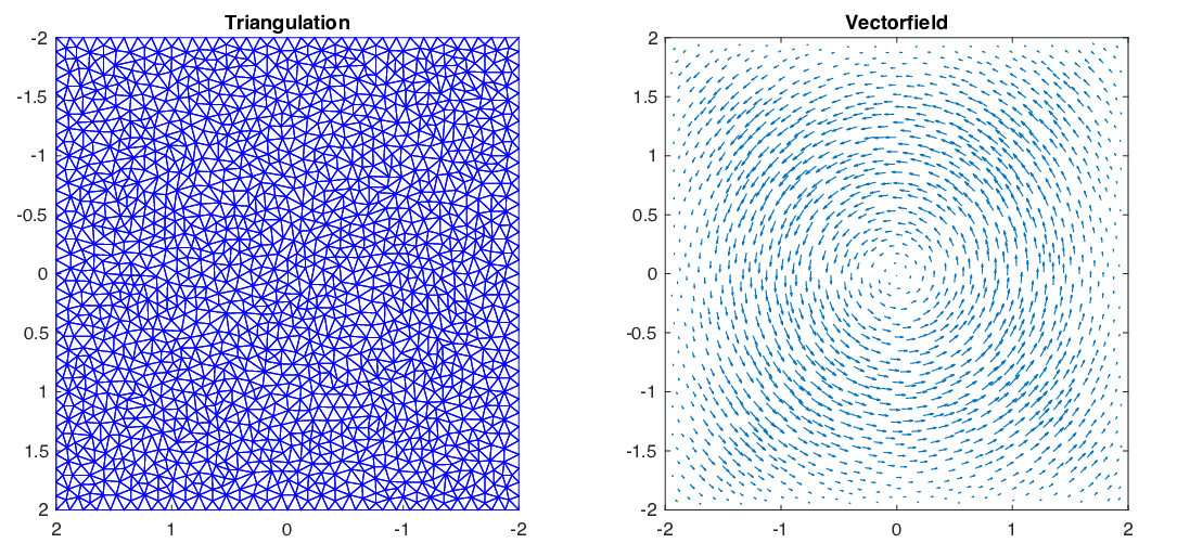
Figure 4: Test 2. Triangulation used (Δ​x=0.08\Delta x=0.08) and vector field bb.
Refer to caption
Figure 5: Test 2. Solution of the transport equation at various moments of its evolution.
Refer to caption
Figure 6: Test 2. Solution of the conservation equation at various moments of its evolution.
Refer to caption
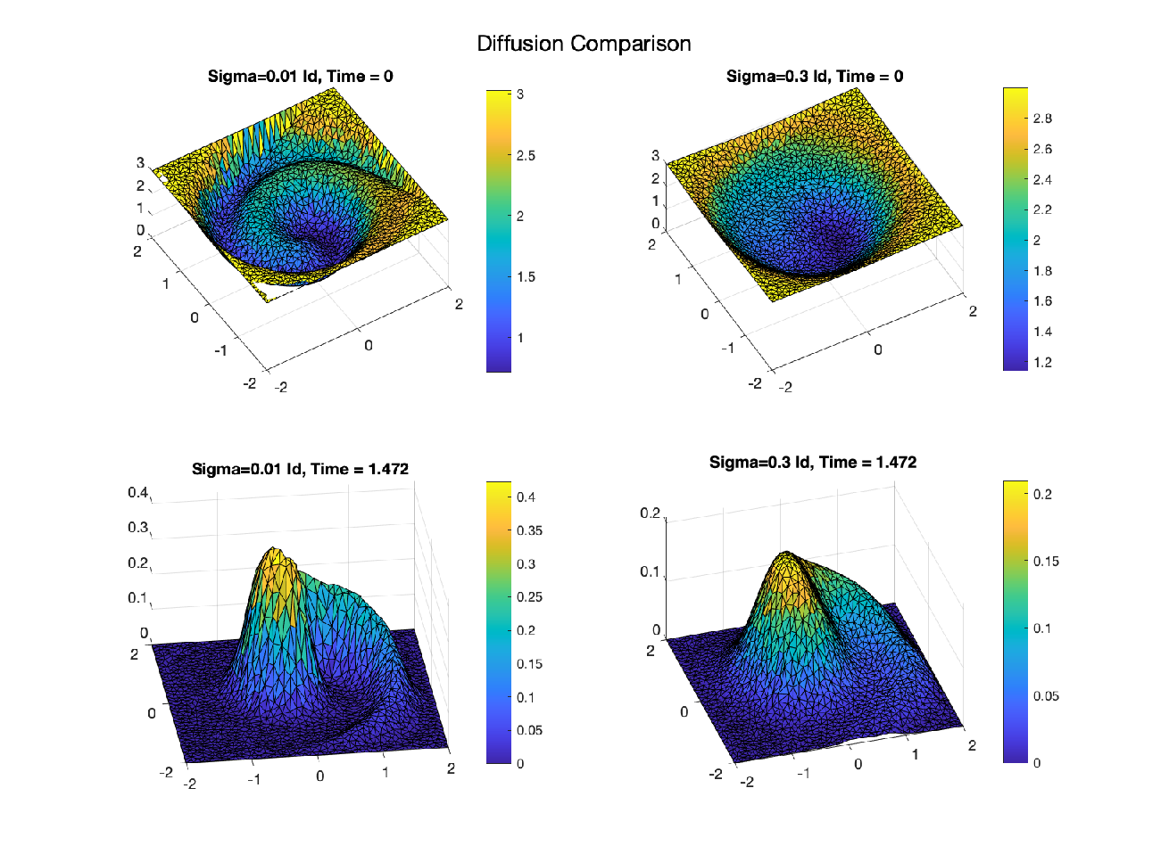
Figure 7: Test 2. Comparison for various choices of σ\sigma: respectively, σ=10−2​Id2\sigma=10^{-2}\text{Id}_{2} (left) and σ=0.3​Id2\sigma=0.3\,\text{Id}_{2} (right).

In the second test, we move to a two-dimensional case. The aim is to study the properties of the scheme with respect to a triangular grid. We consider a problem set in [−2,2]2⊂ℝ2[-2,2]^{2}\subset\mathbb{R}^{2}, with a continuous drift

−b⁡(t,x)=(2−max⁡(|x1|,|x2|))​(x2,−x1),-b(t,x)=(2-\max(|x_{1}|,|x_{2}|))\,(x_{2},-x_{1}),

a rotating velocity field that degenerates near the origin and along the boundary of [−2,2]2[-2,2]^{2} (see Figure 4). For this domain, we employ a triangular mesh generator with Δ​x=0.08\Delta x=0.08 (corresponding to the maximum triangle area). The mesh is generated using the well-known software Triangle [27], which produces a quality, conforming Delaunay triangulation of bounded 2D domains.

The other problem parameters are set as follows: h=2​Δ​xh=2\Delta x and a⁡(t,x)≡12​σ​σTa(t,x)\equiv\frac{1}{2}\sigma\sigma^{T}, with σ=10−3​Id2\sigma=10^{-3}\,\text{Id}_{2}, where Id2\text{Id}_{2} is the identity matrix of dimension 2. The time interval is [0,T]=[0,1.5][0,T]=[0,1.5]. In this case, we take as mollifier the standard bivariate distribution

ρ⁡(x):=12​π​exp⁡(−12​(x12+x22)).\rho(x):=\frac{1}{2\pi}\exp\left(-\frac{1}{2}(x_{1}^{2}+x_{2}^{2})\right).

We begin by considering the backward viscous transport equation with final condition

uT​(x)=(x1−1)2+x22.u_{T}(x)=\sqrt{(x_{1}-1)^{2}+x_{2}^{2}}.

Figure 5 shows the approximate solution at different times during its evolution. In this case, the presence of a nondifferentiable point in the final condition (only Lipschitz continuity is required by Theorem 4.4) does not affect the performance of the numerical scheme, which successfully approximates the solution without introducing spurious oscillations.

We now turn to analyzing the same choice of parameters for the viscous conservation equation, with initial condition

f0​(x)=𝟙[−1.5,−0.1]×[−0.25,0.25]​(x),f_{0}(x)=\mathbbm{1}_{[-1.5,-0.1]\times[-0.25,0.25]}(x),

where the initial data is clearly discontinuous. Figure 6 displays the approximate solution at various times during its evolution. It is possible to observe that a higher density remains concentrated near the center of the domain (where the vector field bb is smaller), while the rest of the density moves more rapidly in a non-uniform circular motion.

In Figure 7 we observe how various choices of the diffusion coefficient σ\sigma influences the solution. We report here the previous test with, respectively, σ=10−2​Id2\sigma=10^{-2}\text{Id}_{2} (left) and σ=0.3​Id2\sigma=0.3\,\text{Id}_{2} (right).

Refer to caption
Figure 8: Test 3. Transport equation. The red line marks the position, varying in time, of the discontinuity in the velocity field. The contour lines are also displayed for a better interpretation of the plot.
Refer to caption
Figure 9: Test 3. Conservation equation. The red line marks the position, varying in time, of the discontinuity in the velocity field. The initial density concentrates while passing through the moving discontinuity.

Test 3

In our third test we pass to the case of a discontinuous velocity field bb, time-varying, that verifies the (OSLC) condition. We consider

−b⁡(t,x,y)={(3/2,0)x<t(1/2,0)x≥t-b(t,x,y)=\begin{cases}(3/2,0)\quad&x<t\\ (1/2,0)\quad&x\geq t\end{cases}

where we can notice that the discontinuity moves in the same direction of the motion with unitary speed, while beyond the discontinuity, since the speed is lower, we expect then that a compression wave will appear. In this test the diffusion coefficient is variable, while the scenario remains convection dominant. We set

σ⁡(t,x)=0.1​|cos⁡(π​x1)​cos⁡(π​x2)|​Id2\sigma(t,x)=0.1\,|\cos(\pi\,x_{1})\cos(\pi\,x_{2})|\,\text{Id}_{2}

where we observe that such function degenerate to zero in some points of the domain.

In Figure 8 we observe the (backward) evolution of the viscous transport equation in the time interval [0,0.8][0,0.8], starting from the final condition

uT​(x)=(x1−0.8)2+x22.u_{T}(x)=\sqrt{(x_{1}-0.8)^{2}+x_{2}^{2}}.

Here the discretization parameters are set as (Δ​x,h)=(0.01,0.02)(\Delta x,h)=(0.01,0.02). In the figure, the red line marks the position of the discontinuity in the velocity field bb. Such discontinuity is visible in the gradient of the approximated solution, while the diffusion tends to smooth up the minimum point of the initial solution. Also in this case, to avoid boundary effects, the problem is computed in a much larger domain (in particular [−4,4]2[-4,4]^{2}).

We now turn to analyzing the same choice of parameters for the viscous conservation equation, with initial condition

f0​(x)=𝟙[−1,1]×[−0.5,0.5]​(x).f_{0}(x)=\mathbbm{1}_{[-1,1]\times[-0.5,0.5]}(x).

Figure 9 shows the approximate solution at several time points during its evolution. A compression wave can be observed, as indicated by the fact that the peak concentration at the final time exceeds the maximum of the initial condition. This concentration effect is smoothed by diffusion and by the fact that the discontinuity propagates in the same direction as the drift.

7 Conclusions

In this work, we developed and analyzed semi-Lagrangian schemes on unstructured meshes for viscous transport and conservative equations with coefficients satisfying a one-sided Lipschitz condition. By leveraging a probabilistic framework and the dual characterization of solutions as viscosity and duality solutions, we proved convergence under minimal regularity assumptions. The schemes exhibit strong robustness in the presence of irregular data and extend classical semi-Lagrangian methods beyond the Di Perna-Lions setting.

Numerical results confirm convergence to the correct solution and validate the method’s accuracy and stability on unstructured grids, making it particularly effective for high-dimensional and geometrically complex domains. The approach is especially relevant for Mean Field Games, where monotone interactions and degenerate dynamics frequently arise. Its compatibility with measure-theoretic formulations and probabilistic interpretations enhances its suitability for modeling socio-economic and collective behavior dynamics.

Future directions include extending the method to fully nonlinear second-order equations and systems with additional couplings or controls.

References

  • [1] Ambrosio, L. Transport equation and Cauchy problem for BV vector fields. Invent. Math. 158 (2004), no. 2, 227–260.
  • [2] Barles, G. A new stability result for viscosity solutions of nonlinear parabolic equations with weak convergence in time. C. R. Math. Acad. Sci. Paris 343 (2006), no.3, 173–178.
  • [3] Barles, G.; Souganidis, P. E. Convergence of approximation schemes for fully nonlinear second order equations. Asymptotic Anal. 4 (1991), no. 3, 271–283.
  • [4] Bonaventura, L.; Ferretti, R. Semi-Lagrangian methods for parabolic problems in divergence form. SIAM J. Sci. Comput., 36 (2014), no. 5, A2458–A2477.
  • [5] Bouchut, F.; James, F. One-dimensional transport equations with discontinuous coefficients. Nonlinear Anal. 32 (1998), no. 7, 891–933.
  • [6] Bouchut, F.; James, F.; Mancini, S. Uniqueness and weak stability for multi-dimensional transport equations with one-sided Lipschitz coefficient. Ann. Sc. Norm. Super. Pisa Cl. Sci. (5) 4, 1 (2005), 1–25.
  • [7] Cacace, S.; Cristiani, E.; Ferretti, R. Blended numerical schemes for the advection equation and conservation laws. ESAIM: Math. Model. Numer. Anal., 51 (2017) no. 3, 997–1019.
  • [8] Camilli, F.; Falcone, M. An approximation scheme for the optimal control of diffusion processes. RAIRO Modél. Math. Anal. Numér. 29 (1995), no. 1, 97–122.
  • [9] Cardaliaguet P.; Forcadel N.; Girard T.; Monneau R. Conservation laws and Hamilton-Jacobi equations on a junction: The convex case. Discrete Contin. Dyn. Syst., 44 (224) no. 12, 3920–3961.
  • [10] Cardaliaguet, P.; Souganidis, P. E. On first order mean field game systems with a common noise. Ann. Appl. Probab. 32 (2022), no. 3, 2289–2326.
  • [11] Carlini, E.; Silva, F. J. A semi-Lagrangian scheme for a degenerate second order mean field game system. Discrete Contin. Dyn. Syst. 35 (2015), no. 9, 4269–4292.
  • [12] Carlini, E.; Silva, F. J. On the discretization of some nonlinear Fokker-Planck-Kolmogorov equations and applications. SIAM J. Numer. Anal. 56 (2018), no. 4, 2148–2177.
  • [13] Delarue, F.; Lagoutière, F. Probabilistic analysis of the upwind scheme for transport equations. Arch. Ration. Mech. Anal. 199 (2011), no. 1, 229–268.
  • [14] Delarue, F.; Lagoutiere, F.; Vauchelet, N. Convergence order of upwind type schemes for transport equations with discontinuous coefficients. J. Math. Pures Appl. 108(2017), no.6, 918–951.
  • [15] DiPerna, R. J.; Lions, P.-L. Ordinary differential equations, transport theory and Sobolev spaces. Invent. Math. 98 (1989), no. 3, 511–547.
  • [16] Falcone, M.; Ferretti, R. Semi-Lagrangian approximation schemes for linear and Hamilton-Jacobi equations. Society for Industrial and Applied Mathematics (SIAM), Philadelphia, PA, 2014, xii+319 pp.
  • [17] Figalli, A. Existence and uniqueness of martingale solutions for SDEs with rough or degenerate coefficients. J. Funct. Anal. 254 (2008), no. 1, 109–153.
  • [18] Festa, A.; Göttlich, S.; Pfirsching, M. A model for a network of conveyor belts with discontinuous speed and capacity. Netw. Heterog. Media, 14 (2019), no. 2, 389—410.
  • [19] Friedrich, J.; Göttlich, S.; Uphoff, A. Conservation laws with discontinuous flux function on networks: a splitting algorithm. Netw. Heterog. Media 18(2023), no. 1, 1-28.
  • [20] Gosse, L.; James, F. Numerical approximations of one-dimensional linear conservation equations with discontinuous coefficients, Math. Comput. 69 (2000), 987–1015.
  • [21] Le Bris, C.; Lions, P.-L. Existence and uniqueness of solutions to Fokker-Planck type equations with irregular coefficients. Comm. Partial Differential Equations 33 (2008), 1272–1317.
  • [22] Lions, P.-L. ; Perthame, B. Remarks on Hamilton-Jacobi equations with measurable time-dependent Hamiltonians. Nonlinear Anal. 11 (1987), no.5, 613–621.
  • [23] Lions, P.-L.; Seeger, B. Transport Equations and Flows with One-Sided Lipschitz Velocity Fields. Arch. Ration. Mech. Anal. 248 (2024), no.5, Paper No. 86.
  • [24] Monteillet, A. Convergence of approximation schemes for nonlocal front propagation equations. Math. Comp. 79 (2010), no.269, 125–146.
  • [25] Navarro-Fernández, V.; Schlichting, A. Error estimates for a finite volume scheme for advection-diffusion equations with rough coefficients. ESAIM Math. Model. Numer. Anal. 57 (2023), no. 4, 2131–2158.
  • [26] Poupaud, F.; Rascle, M. Measure solutions to the linear multi-dimensional transport equation with non-smooth coefficients. Comm. Partial Differential Equations 22, (1997), no. 1-2, 337–358.
  • [27] Shewchuk, J.R. Triangle: Engineering a 2D quality mesh generator and Delaunay triangulator. In “Applied Computational Geometry: Towards Geometric Engineering”, vol. 1148, Lecture Notes in Computer Science, Springer-Verlag, Berlin, (1996), 203–222. In Workshop on applied computational geometry. Springer Berlin Heidelberg,
  • [28] Villani, C. Optimal transport, old and new, Grundlehren der Mathematischen Wissenschaften 338, Springer, 2009.