QubitLens: An Interactive Learning Tool for Quantum State Tomography

Quantum computing is an emerging technology with the potential to tackle problems that are intractable for classical systems. A fundamental requirement in quantum computing is the ability to accurately prepare, manipulate, and measure quantum states. One critical task in this context is quantum state tomography, a foundational concept in quantum information theory. It involves reconstructing an unknown quantum state by analyzing the outcomes from a set of measurements performed on multiple identical copies of the state.

Quantum state tomography is most commonly introduced in graduate-level courses, as it involves several technically demanding concepts. These include the density matrix formalism, partial trace operations, quantum channels, and the generalized framework of quantum measurement  [1, 2, 3]. While foundational, these concepts can pose a steep learning curve for students who are just beginning to learn about quantum computing. There have been numerous well-established methods for quantum state tomography, including linear inversion [4], Bayesian estimation [5], and maximum likelihood estimation (MLE) [6, 7]. Other approaches, such as compressed sensing [8] and neural-network-based tomography [9], have also been proposed to improve scalability and accuracy in high-dimensional settings. Although powerful, these methods often require an advanced background in quantum mechanics, statistics, and optimization theory, which makes them less approachable for beginners or for educational purposes.

In this work, we introduce QubitLens, an interactive and educational tool designed to help students and educators better understand the basic principles of quantum state tomography. QubitLens focuses on pure-state tomography for single and multi-qubit systems, using MLE as a backend algorithm. Importantly, the tool avoids complicated density matrix manipulations and instead emphasizes intuitive, visual elements such as Bloch sphere representations and bar plots to assess reconstruction quality. By making the learning process hands-on and visually guided, QubitLens offers a more approachable path for beginners to engage with one of the most essential ideas in quantum information theory.

This paper is structured as follows. We first introduce the concept of MLE in a simple and accessible way. Since MLE is a common statistical method often taught in high school or early undergraduate courses, we show how it can be naturally extended to quantum state estimation. Next, we provide the necessary background in quantum computing, with a particular focus on measurements performed in different Pauli bases for a single qubit. Following this, we present QubitLens, and finally, we extend our framework to accommodate the multi-qubit scenario.

Maximum likelihood estimation (MLE) is a fundamental statistical technique used to estimate unknown parameters of a probability distribution from observed data. Consider a parametric family of probability distributions $\{P_{\boldsymbol{\theta}}\}$ indexed by a parameter vector $\boldsymbol{\theta}$. We have given a dataset $\mathcal{D}$ which is assumed to be independently and identically distributed (i.i.d.) according to $P_{\boldsymbol{\theta}_{\text{true}}}$, where $\boldsymbol{\theta}_{\text{true}}$ is the true but unknown parameter. The goal of MLE is to find the parameter $\hat{\boldsymbol{\theta}}$ that maximizes the likelihood of the observed data. Formally,

where $\mathcal{L}(\boldsymbol{\theta};\mathcal{D})$ denotes the likelihood function, i.e., the probability of observing the data $\mathcal{D}$ under the distribution parameterized by $\boldsymbol{\theta}$. In practice, the logarithm of the likelihood, known as the log-likelihood, is typically used instead of the likelihood for both analytical and numerical convenience.

To illustrate this process concretely, we consider three mutually independent binary random variables $\mathsf{X}$, $\mathsf{Y}$, and $\mathsf{Z}$, each taking values in $\{+1,-1\}$. We model these using Bernoulli random variables, where a success corresponds to observing $+1$. The probability of success for each variable is assumed to depend on a shared underlying parameter vector $\boldsymbol{\theta}$, with $p_{\text{X}}(\boldsymbol{\theta})$, $p_{\text{Y}}(\boldsymbol{\theta})$, and $p_{\text{Z}}(\boldsymbol{\theta})$ denoting the corresponding success probabilities.

Suppose we observe $N_{\text{X}}$, $N_{\text{Y}}$, and $N_{\text{Z}}$ i.i.d. samples according to $p_{\text{X}}(\boldsymbol{\theta})$, $p_{\text{Y}}(\boldsymbol{\theta})$, and $p_{\text{Z}}(\boldsymbol{\theta})$, respectively, denoted by:

The number of observed successes for each variable is:

where $\mathbf{1}_{\{\mathcal{E}\}}$ denotes the indicator function, which equals $1$ if the event $\mathcal{E}$ occurs and $0$ otherwise. The likelihood function for each variable is based on the Bernoulli model:

Since $\mathsf{x}_{i}$, $\mathsf{y}_{i}$, and $\mathsf{z}_{i}$ are i.i.d., the joint likelihood over all observations is simply the product of the individual likelihoods:

Taking the logarithm yields the total log-likelihood:

To estimate the parameter vector $\boldsymbol{\theta}$, one maximizes the log-likelihood function using numerical optimization methods. Depending on the form of $p_{\text{X}}(\boldsymbol{\theta})$, $p_{\text{Y}}(\boldsymbol{\theta})$, and $p_{\text{Z}}(\boldsymbol{\theta})$, this optimization may be performed using gradient-based methods (e.g., gradient descent or ADAM) or gradient-free methods such as COBYLA or L-BFGS [10]. These algorithms iteratively update the $\boldsymbol{\theta}$ (parameter estimate) to approach the $\boldsymbol{\theta}_{\text{true}}$.

A qubit is the quantum counterpart of a classical bit, capable of existing in a coherent superposition of the binary values $0$ and $1$. Unlike a classical bit, which deterministically assumes a value of either $0$ or $1$ at any given time, a qubit is described by a column vector in a two-dimensional complex Hilbert space. Mathematically, a single qubit state is expressed as a linear combination of two orthonormal basis states, conventionally denoted in Dirac notation as $|0\rangle\text{ and }|1\rangle$, with corresponding column vector representations:

The orthonormal basis states $|0\rangle\text{ and }|1\rangle$ are commonly referred to as the computational basis. An arbitrary (pure) qubit state can be written as a superposition of these basis states:

where $\alpha,\beta\in\mathbb{C}$ are complex probability amplitudes satisfying the normalization condition: $|\alpha|^{2}+|\beta|^{2}=1$. The conjugate transpose of this state, denoted as $\langle\psi|$, is given as a row vector

where $\alpha^{*}$ and $\beta^{*}$ are the complex conjugate of $\alpha\text{ and }\beta$, respectively. This row vector form allows one to compute expressions like the inner product $\langle\psi|\psi\rangle=|\alpha|^{2}+|\beta|^{2}=1$, which confirms that the state is properly normalized.

We now present the algorithm for performing single-qubit state tomography using the MLE. Alongside the conceptual description, we provide corresponding code snippets for each step to enhance understanding. The code is implemented in Python 3 using NumPy, matplotlib, ipywidgets, and QuTiP libraries.

The algorithm takes the true parameters $\theta_{\text{true}}$ and $\phi_{\text{true}}$ as inputs, along with the number of measurement shots $N_{\text{X}},N_{\text{Y}},\text{ and }N_{\text{Z}}$ for the $\mathbf{X},\mathbf{Y},\text{ and }\mathbf{Z}$ bases, respectively. Below, we detail each step involved in the algorithm.

We embed the above qubit state tomography using the MLE algorithm within an interactive visualization tool we refer to as QubitLens. This tool is designed to provide intuitive insights into the process of single-qubit state tomography by exposing the algorithmic workflow through an interactive front end. Users can specify the true state parameters $(\theta_{\text{true}},\phi_{\text{true}})$ using sliders, and independently choose the number of measurement shots in each Pauli basis ($N_{\text{X}},N_{\text{Y}},N_{\text{Z}}$). Upon adjusting these inputs, the interface dynamically updates three visual components: (i) a side-by-side Bloch sphere visualization of the true state and the reconstructed state, (ii) a bar plot comparing the true and estimated values of $\theta$ and $\phi$, and (iii) a fidelity gauge indicating the closeness of the reconstructed state to the true state (see Fig. 2).

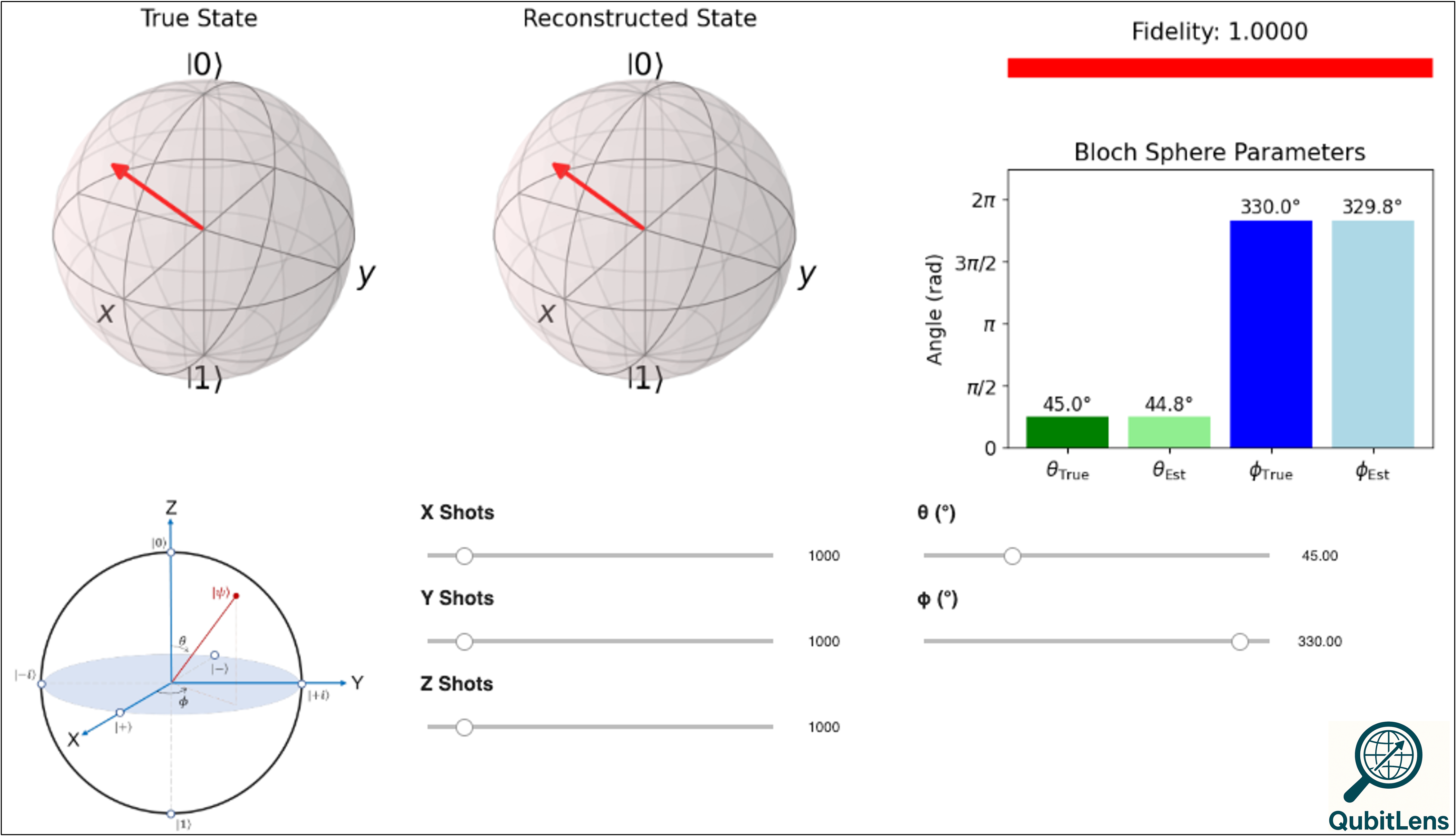
The Qubit Lens framework allows users to explore how measurement choices affect the reconstruction of quantum states. For instance, as detailed in Section III-C, when measurements are restricted to the $\mathbf{Z}$ basis alone, only information about $\theta$ can be recovered; the reconstructed state is necessarily insensitive to variations in $\phi$ as shown in Fig. 3.

When measurements are taken in both the $\mathbf{X}$ and $\mathbf{Z}$ bases, the polar angle $\theta$ can be reliably estimated, but ambiguity still remains in determining the azimuthal angle $\phi$. In particular, the tomography algorithm can yield either $\hat{\phi}=\phi_{\text{true}}$ or $\hat{\phi}=2\pi-\phi_{\text{true}}$. This behavior is illustrated in Fig. 4, where the top part shows the case where the algorithm outputs $\hat{\phi}=2\pi-\phi_{\text{true}}$, while in the bottom part the algorithm returns $\hat{\phi}=\phi_{\text{true}}$. To accurately estimate the parameters, it is essential to include measurements from all three Pauli bases because measurements in the $\mathbf{Y}$ basis provide information about $\sin(\phi)$, which helps to break the ambiguity and allows for the precise estimation of $\phi$, as shown in Fig. 2.

In this section, we extend the algorithm to multi-qubit systems. To illustrate this extension, we first describe how pure multi-qubit states can be parametrized using generalized polar coordinates, which form the foundation for the likelihood-based reconstruction procedure.

An arbitrary pure state of $n$ qubits can be represented as a unit vector in a $2^{n}-$dimensional complex Hilbert space. To ensure normalization and avoid redundancy due to the global phase, the state can be parametrized using a sequence of generalized polar coordinates as:

where $c=(2^{n}-1)$, the angles $\boldsymbol{\theta}=(\theta_{1},\theta_{2},\ldots,\theta_{c})$ and phases $\boldsymbol{\phi}=(\phi_{1},\phi_{2},\ldots,\phi_{c})$ completely specify the pure state, with $\theta_{i}\in[0,\pi]$ and $\phi_{i}\in[0,2\pi)$. This parametrization ensures that the unit norm constraint $\langle\psi(\boldsymbol{\theta},\boldsymbol{\phi})|\psi(\boldsymbol{\theta},\boldsymbol{\phi})\rangle=1$ is automatically satisfied.

References

- [1] M. A. Nielsen and I. L. Chuang, Quantum Computation and Quantum Information: 10th Anniversary Edition. Cambridge University Press, 2010.
- [2] M. G. A. Paris and J. Řeháček, Eds., Quantum State Estimation, ser. Lecture Notes in Physics. Springer, 2004, vol. 649.
- [3] M. M. Wilde, Quantum information theory. Cambridge university press, 2013.
- [4] G. M. D’ARIANO, “Quantum tomography g. mauro d’ariano, matteo ga paris, and massimiliano f. sacchi,” Advances in imaging and electron physics, vol. 128, p. 205, 2003.
- [5] R. Blume-Kohout, “Optimal, reliable estimation of quantum states,” New Journal of Physics, vol. 12, no. 4, p. 043034, 2010.
- [6] Z. Hradil, “Quantum-state estimation,” Phys. Rev. A, vol. 55, pp. R1561–R1564, 1997.
- [7] J. Řeháček, Z. Hradil, E. Knill, and A. Lvovsky, “Diluted maximum-likelihood algorithm for quantum tomography,” Physical Review A—Atomic, Molecular, and Optical Physics, vol. 75, no. 4, p. 042108, 2007.
- [8] D. Gross, Y.-K. Liu, S. T. Flammia, S. Becker, and J. Eisert, “Quantum state tomography via compressed sensing,” Physical review letters, vol. 105, no. 15, p. 150401, 2010.
- [9] G. Torlai, G. Mazzola, J. Carrasquilla, M. Troyer, R. Melko, and G. Carleo, “Many-body quantum state tomography with neural networks,” arXiv preprint arXiv:1703.05334, 2017.
- [10] J. Nocedal and S. J. Wright, Numerical optimization. Springer, 1999.
- [11] Qiskit, “plot_bloch_multivector: Visualize bloch vectors of multiqubit states,” https://docs.quantum.ibm.com/api/qiskit/qiskit.visualization.plot_bloch_multivector, 2024, accessed: 2025-05-10.