跳到论文正文
W Papers独立论文阅读器 arXiv:2505.07482 论文正文 计算阅读时间 · 0%
引用这篇论文根据当前论文元数据生成,正式投稿前建议核对。


License: arXiv.org perpetual non-exclusive license
arXiv:2505.07482v2 [math.OC] 02 Jan 2026

Enhancing Accuracy in Differentially Private Distributed Optimization Through Sensitivity Reduction

Furan Xie    Bing Liu    Li Chai ††thanks: This work was supported in part by the National Natural Science Foundation of China under Grant 62573332 and Grant U2441244, and in part by the Zhejiang Provincial Natural Science Foundation of China under Grant LZ24F030006. (Corresponding author: Bing Liu and Li Chai).††thanks: Furan Xie and Bing Liu are with the Engineering Research Center of Metallurgical Automation and Measurement Technology, Wuhan University of Science and Technology, Wuhan 430081, China (e-mail: xiefuran328@qq.com; liubing17@wust.edu.cn).††thanks: Li Chai is with the State Key Laboratory of Industrial Control Technology, College of Control Science and Engineering, Zhejiang University, Hangzhou 310027, China (e-mail: chaili@zju.edu.cn).
Abstract

In this paper, we investigate the problem of differentially private distributed optimization. Recognizing that lower sensitivity leads to higher accuracy, we analyze the key factors influencing the sensitivity of differentially private distributed algorithms. Building on these insights, we propose a novel differentially private distributed algorithm for undirected graphs that enhances optimization accuracy by reducing sensitivity. To ensure practical applicability, we derive an explicit closed-form expression for the noise parameter as a function of the privacy budget. Moreover, we rigorously prove that the proposed algorithm can achieve arbitrarily rigorous ϵ\epsilon-differential privacy, establish its convergence in the mean square sense, and provide an upper bound on its optimization accuracy. Finally, extensive comparisons with various privacy-preserving methods validate the effectiveness of our algorithm.

Index Terms: 
Distributed optimization, privacy preservation, differential privacy, sensitivity, gradient tracking

I Introduction

With the widespread application of distributed optimization in various fields such as machine learning, power systems, and robotic networks, the growing sophistication of cyberattacks has brought security and privacy concerns to the forefront of research [1]. Compared to traditional centralized approaches, distributed optimization methods offer better privacy protection by avoiding the direct exchange of raw data, which may contain sensitive information. Nevertheless, studies have shown that the exchange of states and (estimated) gradients between agents in distributed optimization can still pose significant privacy risks. For instance, in distributed machine learning, attackers can accurately recover an agent’s raw data through its gradient [2]. In the distributed rendezvous problem, an agent’s state itself is its sensitive information [3]. Therefore, how to design distributed optimization methods that can protect the sensitive information of agents has become an urgent challenge.

In general, privacy-preserving distributed optimization algorithms can be categorized into three types: correlated randomness-based methods, encryption-based methods, and differential privacy-based methods.

Correlated randomness-based methods achieve privacy protection by introducing temporally or spatially correlated randomness into the optimization process. [4] and [5] protect agents’ private information by injecting structured random noise adhering to a zero-sum structure into the interactive messages between agents. [6] further strengthens privacy by simultaneously introducing functional and state perturbations that also satisfy a zero-sum constraint. [7] safeguards agents’ privacy by injecting random noise into the dual variables directed towards a non-convergent subspace. [8] protects the privacy of agents’ gradients by adding randomness to the stepsizes and coupling weights during the initial iterations. [9] and [10], on the other hand, utilize state decomposition techniques to split the local state into public and private substates, transmitting only the substate unrelated to private information during communication, thereby achieving privacy preservation. Leveraging the robustness of the system dynamics, these methods can attain exact convergence. However, they require an additional topological assumption to ensure privacy protection and cannot defend against external eavesdroppers.

In contrast, encryption-based methods can effectively defend against external eavesdroppers by encrypting the transmitted information. [11] and [12] propose two privacy-preserving distributed optimization algorithms by integrating the Alternating Direction Method of Multipliers (ADMM) and Distributed Gradient Descent (DGD) methods with Homomorphic Encryption (HE). Considering the significant computational and communication overhead associated with HE, several efficiency optimization techniques can be adopted to mitigate these burdens. [13] combines quantization techniques with HE, significantly reducing the size of data to be encrypted and transmitted by converting high-precision gradients into low-bit integers. [14] integrates packing (batching) techniques with HE, reducing communication frequency by aggregating multiple data elements into a single plaintext or ciphertext before encryption and transmission. Moreover, replacing HE with lightweight cryptographic primitives, such as the Advanced Encryption Standard (AES) in [15] and functional encryption in [16], can reduce the overall computational and communication burden. Despite these advances, compared to other types of privacy-preserving methods, the encryption and decryption operations in encryption-based approaches still introduce additional computational or communication overhead.

Due to the wide applicability, simplicity, and strong theoretical privacy guarantees, Differential Privacy (DP) has emerged as the de facto standard for privacy protection in recent years [17]. Several studies have integrated DP into distributed optimization by injecting random noise into the information transmitted between agents. [18] proposes a differentially private algorithm based on DGD, under the assumption that the gradients of all individual cost functions are bounded. However, since DGD relies on inexact gradients, its convergence rate remains sublinear, even without the addition of DP noise. In contrast, the Gradient Tracking (GT) algorithms can achieve linear convergence with a constant stepsize [19]. To this end, [20] presents a differentially private GT algorithm that achieves linear convergence over undirected graphs. This result is later extended to time-varying directed graphs by [21]. Both works, however, rely on the assumption that different objective functions in two adjacent problems share the same Lipschitz constant and convexity parameter. On the other hand, [18], [20], and [21] all reveal the inherent trade-off between privacy and accuracy in differentially private algorithms.

To optimize the privacy-accuracy trade-off in differentially private algorithms, various techniques have been proposed. [22] presents a GT-based distributed algorithm that ensures both DP and optimality by incorporating decaying weakening factors into weight matrices. However, to achieve rigorous DP, this method requires the assumption that adjacent objective functions have consistent gradients within the neighborhood of the optimal solution. In addition, in the presence of persistent DP noise, GT techniques suffer from noise accumulation, which negatively impacts the algorithm’s accuracy. To mitigate this issue, [23] proposes a differentially private distributed algorithm based on Robust Gradient Tracking (RGT) for undirected graphs. [24] later extends this approach to directed graphs. [25] proposes a distributed algorithm that integrates RGT with decaying weakening factors, ensuring almost sure convergence in the presence of information-sharing noise. As an enhancement, [26] further incorporates a variance reduction technique into this framework, which reduces the estimation error variance and relaxes the assumptions on network connectivity. However, whether these two methods can provide rigorous DP guarantees remains unclear.

Apart from the aforementioned research focused on suppressing or reducing the impact of noise, another line of work aims to optimize the noise itself, with the core idea being to dynamically adjust the scale and distribution of noise based on the characteristics of the model or data. The adaptive noise mechanism is a typical representative of this direction. For instance, in the federated learning setting, [27] proposes a method combining adaptive gradient clipping and adaptive noise scaling, which better aligns the noise with the training phase and client heterogeneity. Furthermore, [28] introduces a component-wise adaptive noise mechanism that takes into account the heterogeneity in parameter magnitudes. By estimating the sensitivity of each parameter component and adding Gaussian noise scaled accordingly, this approach prevents excessive distortion to parameters with smaller magnitudes. On the other hand, from the perspective of system and communication architecture, introducing the shuffle model to achieve “privacy amplification” has emerged as another important approach to enhance privacy. This model incorporates an anonymization step: users first perturb their data locally, after which a trusted shuffler randomly permutes all user messages before sending them to the analyzer. This process severs the association between outputs and their senders, thereby providing stronger central DP guarantees for aggregated results compared to pure local perturbation [29, 30, 31]. However, how to apply adaptive noise mechanisms and privacy amplification strategies to general differentially private decentralized optimization remains an open problem requiring in-depth research.

Despite significant advancements in differentially private distributed optimization, several critical challenges remain. Firstly, existing differentially private algorithms lack clear design principles to systematically improve accuracy, as well as theoretical frameworks to validate such improvements. As a result, efforts to enhance accuracy often rely on heuristic tuning rather than guided optimization, and it remains challenging to rigorously discern whether a modification truly improves performance or merely shifts the trade-off elsewhere. Secondly, while relationships between privacy and noise have been studied, there remains a lack of an explicit, closed-form expression that can directly translate a desired privacy budget into actionable noise parameters prior to execution. This makes it difficult to configure algorithms predictably and limits their practical deployment. Thirdly, the use of diminishing stepsizes introduces a fundamental analytical hurdle: the resulting state transition matrix of the algorithm no longer has a spectral radius strictly less than 1. This, combined with persistent noise injection, invalidates standard convergence analysis techniques, making it difficult to establish rigorous performance guarantees. To address these challenges, this paper proposes corresponding solutions, which, along with the contributions of this work, are summarized as follows:

1) A Systematic, Sensitivity-Reduced Design for Accuracy Enhancement. To overcome the lack of design principles, we first reveal that algorithm sensitivity is the key determinant of accuracy under a fixed privacy budget. This novel perspective enables the systematic derivation of design principles for sensitivity reduction (Proposition 1). Implementing these principles, we propose an implicit gradient tracking-based differentially private distributed algorithm for undirected graphs that inherently achieves lower sensitivity. Both theoretical analysis and experiments confirm that the proposed algorithm achieves higher accuracy under the same privacy budget compared to existing methods in [20, 21, 23, 22, 24].

2) An Explicit, Direct Noise Calibration Rule and Halved Overhead. To address the impracticality of implicit noise-privacy relationships, we derive an explicit, directly usable closed-form expression for the noise parameter as a function of the privacy budget. This expression serves as a direct design tool, enabling the exact computation of noise parameters from any given privacy budget before execution. Additionally, the proposed algorithm halves both the number of communication variables and noise injections compared to existing methods in [20, 21, 23, 22, 24], significantly reducing communication and computational overhead.

3) Theoretical Analysis of ϵ\epsilon-DP and Convergence. We prove that the proposed algorithm with appropriate parameters can achieve rigorous ϵ\epsilon-DP under a weak gradient dissimilarity condition (Theorem 1). Furthermore, to address the analytical difficulty arising from diminishing stepsizes and persistent noise, specifically, the resulting non-contractive dynamics, we develop an analysis framework to establish mean-square convergence and derive an upper bound on the optimization accuracy (Theorem 2). This bound explicitly quantifies the privacy-accuracy trade-off. Based on the theoretical results, we provide two practical parameter tuning strategies.

The remainder of this paper is organized as follows. Section II presents the problem formulation and provides relevant definitions of DP. Section III proposes a differentially private distributed algorithm with lower sensitivity. Sections IV and V analyze the DP guarantees and convergence of the proposed algorithm, respectively. Section VI validates the effectiveness of the proposed algorithm through numerical simulations. Finally, Section VII concludes the paper.

Notation: Table I lists the key notations used in this paper; others are defined in their respective sections.

TABLE I: Summary of Key Notations
Symbol Meaning
A. Key Problem and Algorithmic Parameters
nn Number of agents
pp Dimension of the decision variable
fif_{i}, ff Local and global cost functions
𝒙i\bm{x}_{i}, 𝐱\mathbf{x} Local variable of agent ii and stack matrix of all 𝒙i\bm{x}_{i}
𝒙∗\bm{x}^{*} Optimal solution to the global problem
LL, μ\mu Lipschitz smoothness and strong convexity constants
𝒚i\bm{y}_{i} Auxiliary variable for agent ii (not communicated)
𝒛i\bm{z}_{i} Noisy state of agent ii (shared with neighbors)
𝝃i\bm{\xi}_{i} Laplace noise added by agent ii
αk\alpha_{k} Stepsize at iteration kk
β\beta Gain parameter for the auxiliary variable
νk\nu_{k} Parameter of the Laplace noise at iteration kk
ϵ\epsilon Privacy budget
δ\delta Bound on gradient differences for adjacent problems
Δ⁡(k)\Delta(k) Sensitivity of the algorithm at iteration kk
B. General Mathematical Symbols
‖𝒗‖a\|\bm{v}\|_{a} Standard LaL^{a}-norm of vector 𝒗\bm{v}
‖𝒗‖\|\bm{v}\| L2L^{2}-norm of vector 𝒗\bm{v}
‖M‖a\|M\|_{a} Standard induced LaL^{a}-norm of matrix MM
‖M‖\|M\| Frobenius norm of matrix MM
𝟎\mathbf{0}, 𝟏\mathbf{1} All-zeros and all-ones vectors
II Identity matrix
ρ⁡(M)\rho(M) Spectral radius of square matrix MM
ℙ⁡[⋅]\mathbb{P}[\cdot], 𝔼⁡[⋅]\mathbb{E}[\cdot] Probability and expectation operators
L​a​p​(c)Lap(c) Laplace distribution with scale parameter cc

II Problem Formulation

Consider a multi-agent system consisting of nn agents. Each agent ii possesses an individual cost function fi:ℝp→ℝf_{i}:\mathbb{R}^{p}\to\mathbb{R}, which is only known by agent ii itself. All agents perform local computation and communication over an undirected network to collectively minimize:

f⁡(𝒙)≜1n​∑i=1nfi​(𝒙),f(\bm{x})\triangleq\frac{1}{n}\sum_{i=1}^{n}f_{i}(\bm{x}), (1)

where 𝒙∈ℝp\bm{x}\in\mathbb{R}^{p} is the global decision variable and f:ℝp→ℝf:\mathbb{R}^{p}\to\mathbb{R} is the average of all cost functions. This paper aims to protect the privacy of each agent’s local cost function fif_{i}, which constitutes sensitive information. We consider an adversary with arbitrary computational power that can observe all shared information among all agents. This adversary may be an external eavesdropper or any coalition of internal honest-but-curious agents, with knowledge of the network topology, the algorithm’s parameters and rules, and the cost functions of all non-target agents. The privacy objective is to prevent this adversary from inferring the private cost function fif_{i} of any individual agent. Through DP, we ensure the adversary cannot reliably determine the identity or exact form of any agent’s cost function from the algorithm’s outputs. Let 𝒙i\bm{x}_{i} be a local copy of the decision variable for agent ii. Denote the gradient of fif_{i} with respect to 𝒙i\bm{x}_{i} as ∇fi​(𝒙i)\nabla f_{i}(\bm{x}_{i}). For convenience, we further define 𝐱≜[𝒙1,⋯,𝒙n]T∈ℝn×p\mathbf{x}\triangleq\left[\bm{x}_{1},\cdots,\bm{x}_{n}\right]^{T}\in\mathbb{R}^{n\times p} and ∇F​(𝐱)≜[∇f1​(𝒙1),⋯,∇fn​(𝒙n)]T∈ℝn×p\nabla F(\mathbf{x})\triangleq\left[\nabla f_{1}(\bm{x}_{1}),\cdots,\nabla f_{n}(\bm{x}_{n})\right]^{T}\in\mathbb{R}^{n\times p}.

We model an undirected communication network using the graph 𝒢≜(𝒩,ℰ)\mathcal{G}\triangleq(\mathcal{N},\mathcal{E}), where 𝒩≜{1,2,⋯,n}\mathcal{N}\triangleq\{1,2,\cdots,n\} represents the set of agents and ℰ⊆𝒩×𝒩\mathcal{E}\subseteq\mathcal{N}\times\mathcal{N} denotes the set of edges. (i,j)∈ℰ(i,j)\in\mathcal{E} if and only if agents ii and jj can send information to each other. The set of agents that can communicate with agent ii is defined as 𝒩i≜{j∈𝒩:(i,j)∈ℰ}\mathcal{N}_{i}\triangleq\left\{j\in\mathcal{N}:(i,j)\in\mathcal{E}\right\}. Moreover, we employ a nonnegative and symmetric matrix W∈ℝn×nW\in\mathbb{R}^{n\times n} to represent the inter-agent weights. For any i,j∈𝒩i,j\in\mathcal{N}, Wi​j>0W_{ij}>0 if i=ji=j or (i,j)∈ℰ(i,j)\in\mathcal{E}. For all other (i,j)(i,j), Wi​j=0W_{ij}=0. We define 𝒢W≜(𝒩,ℰW)\mathcal{G}_{W}\triangleq(\mathcal{N},\mathcal{E}_{W}) as the graph induced by the weight matrix WW, where (i,j)∈ℰW(i,j)\in\mathcal{E}_{W} if and only if i≠ji\not=j and Wi​j>0W_{ij}>0.

Throughout the paper, we make the following assumptions:

Assumption 1

For each i∈𝒩i\in\mathcal{N}, the individual cost function fif_{i} is LL-smooth and μ\mu-strongly convex, i.e., for any 𝐱,𝐱′∈ℝp\bm{x},\bm{x}^{\prime}\in\mathbb{R}^{p},

‖∇fi​(𝒙)−∇fi​(𝒙′)‖≤L​‖𝒙−𝒙′‖,\displaystyle\|\nabla f_{i}(\bm{x})-\nabla f_{i}(\bm{x}^{\prime})\|\leq L\|\bm{x}-\bm{x}^{\prime}\|,
fi(𝒙′)≥fi(𝒙)+∇fi(𝒙)T(𝒙′−𝒙)+μ2∥𝒙′−𝒙∥2.\displaystyle f_{i}(\bm{x}^{\prime})\geq f_{i}(\bm{x})+\nabla f_{i}(\bm{x})^{T}(\bm{x}^{\prime}-\bm{x})+\frac{\mu}{2}\|\bm{x}^{\prime}-\bm{x}\|^{2}.
Assumption 2

The nonnegative weight matrix WW is symmetric and doubly-stochastic, satisfying W=WTW=W^{T}, 𝟏T​W=𝟏T\bm{1}^{T}W=\bm{1}^{T}, and W​𝟏=𝟏W\bm{1}=\bm{1}. Its induced graph 𝒢W\mathcal{G}_{W} is connected, that is, there exists a path between any two agents.

Remark 1

(On the network topology) Assumption 2 requires the communication graph to be undirected and connected, and the weight matrix to be doubly-stochastic. While this is more restrictive than the directed-graph settings considered in some existing privacy-preserving algorithms (e.g., [22, 24, 21]), it is adopted here to enable a clear investigation of the fundamental challenges in differentially private distributed optimization. Extending the design methodology and theoretical results of this work to directed graphs, which typically rely only on row- or column-stochastic weights, is an important and nontrivial direction for future research.

Next, we introduce some notations. We describe the distributed optimization problem 𝒫\mathcal{P} in (1) using the tuple (𝒳,ℱ,f,𝒢W)(\mathcal{X},\mathcal{F},f,\mathcal{G}_{W}), where 𝒳=ℝp\mathcal{X}=\mathbb{R}^{p} is the domain of optimization. ℱ⊆{𝒳→ℝ}\mathcal{F}\subseteq\{\mathcal{X}\to\mathbb{R}\} is a set of real-valued cost functions. f⁡(𝒙)≜1n​∑i=1nfi​(𝒙)f(\bm{x})\triangleq\frac{1}{n}\sum_{i=1}^{n}f_{i}(\bm{x}) with fi∈ℱf_{i}\in\mathcal{F} for each i∈𝒩i\in\mathcal{N}. 𝒢W\mathcal{G}_{W} is a communication graph induced by the weight matrix WW. We represent a distributed optimization algorithm for solving the problem 𝒫\mathcal{P} by a mapping A​l​g​(𝒫,𝐱⁡(0)):{𝒫,𝐱⁡(0)}→𝒵Alg\left(\mathcal{P},\mathbf{x}(0)\right):\{\mathcal{P},\mathbf{x}(0)\}\to\mathcal{Z}, where 𝐱⁡(0)∈𝒳n\mathbf{x}(0)\in\mathcal{X}^{n} is the initial state of all agents. 𝒵={𝐳⁡(0),𝐳⁡(1),⋯}∈𝕆\mathcal{Z}=\{\mathbf{z}(0),\mathbf{z}(1),\cdots\}\in\mathbb{O} is the sequence of shared information of all agents, also known as the observation sequence, and 𝕆\mathbb{O} denotes the set of all possible observation sequences. Note that since each 𝐳⁡(k)\mathbf{z}(k) takes values in the continuous space 𝒳n\mathcal{X}^{n}, the observation set 𝕆\mathbb{O} is continuous. Furthermore, under a distributed optimization algorithm A​l​gAlg, for 𝒫\mathcal{P}, 𝐱⁡(0)\mathbf{x}(0), and 𝒵\mathcal{Z}, we denote the algorithm’s internal states as S​t​a​(𝒫,𝐱⁡(0),𝒵)Sta(\mathcal{P},\mathbf{x}(0),\mathcal{Z}), which encompass all data and variables that are stored locally by each agent and not directly shared with other agents.

With the above notations, we are ready to present the definitions of adjacency for two distributed optimization problems, and of ϵ\epsilon-DP and sensitivity for a distributed algorithm.

Definition 1

(Adjacency [24]) Two distributed optimization problems 𝒫\mathcal{P} and 𝒫′\mathcal{P}^{\prime} are adjacent, if the following hold:

  1. 1.

    𝒳=𝒳′\mathcal{X}=\mathcal{X}^{\prime}, ℱ=ℱ′\mathcal{F}=\mathcal{F}^{\prime}, and 𝒢W=𝒢W′\mathcal{G}_{W}=\mathcal{G}_{W}^{\prime}.

  2. 2.

    There exists an i0∈𝒩i_{0}\in\mathcal{N} such that fi0≠fi0′f_{i_{0}}\not=f_{i_{0}}^{\prime} and for all j≠i0j\not=i_{0}, fj=fj′f_{j}=f_{j}^{\prime}.

  3. 3.

    The distance between the gradients of fi0f_{i_{0}} and fi0′f_{i_{0}}^{\prime} is bounded by δ\delta on 𝒳\mathcal{X}, i.e., for any 𝒙∈𝒳\bm{x}\in\mathcal{X}, ‖∇fi0​(𝒙)−∇fi0′​(𝒙)‖1≤δ\|\nabla f_{i_{0}}(\bm{x})-\nabla f_{i_{0}}^{\prime}(\bm{x})\|_{1}\leq\delta.

From Definition 1, two distributed optimization problems are adjacent if only one agent modifies its cost function while all other parameters remain unchanged. Furthermore, we require that the distance between the gradients of two different cost functions is bounded. To the best of our knowledge, this condition is the most relaxed in the existing literature, and a detailed discussion is provided in the following remark.

Remark 2

Regarding the condition on different cost functions in adjacent problems, [18] and [23] require that the gradients of all cost functions be bounded, i.e., for any 𝐱∈𝒳\bm{x}\in\mathcal{X} and fi∈ℱf_{i}\in\mathcal{F}, ‖∇fi​(𝐱)‖≤δ1\|\nabla f_{i}(\bm{x})\|\leq\delta_{1} with δ1>0\delta_{1}>0. In contrast, our requirement in Definition 1 is more relaxed, allowing for a broader class of cost functions. For example, the functions fi0​(𝐱)=12​𝐱T​𝐱f_{i_{0}}(\bm{x})=\frac{1}{2}\bm{x}^{T}\bm{x} and fi0′​(𝐱)=12​𝐱T​𝐱+δp​𝐱f_{i_{0}}^{\prime}(\bm{x})=\frac{1}{2}\bm{x}^{T}\bm{x}+\frac{\delta}{p}\bm{x} satisfy our requirement, but their gradients are unbounded on ℝp\mathbb{R}^{p}. Furthermore, [20] and [21] assume that fi0f_{i_{0}} and fi0′f_{i_{0}}^{\prime} share the same Lipschitz and convexity constants. [22] assumes that fi0f_{i_{0}} and fi0′f_{i_{0}}^{\prime} have identical gradients in the neighborhood of the solution of 𝒫\mathcal{P}. These assumptions impose significantly stricter constraints compared to ours.

Definition 2

(ϵ\epsilon-DP) Given an ϵ>0\epsilon>0, a distributed optimization algorithm A​l​gAlg is ϵ\epsilon-differentially private if for any two adjacent distributed optimization problems 𝒫\mathcal{P} and 𝒫′\mathcal{P}^{\prime}, any initial state 𝐱⁡(0)∈𝒳n\mathbf{x}(0)\in\mathcal{X}^{n}, and any set of the observation sequences 𝒪⊆𝕆\mathcal{O}\subseteq\mathbb{O},

ℙ[Alg(𝒫,𝐱(0))∈𝒪]≤eϵℙ[Alg(𝒫′,𝐱(0))∈𝒪],\mathbb{P}\left[Alg\left(\mathcal{P},\mathbf{x}(0)\right)\in\mathcal{O}\right]\leq e^{\epsilon}\mathbb{P}\left[Alg\left(\mathcal{P}^{\prime},\mathbf{x}(0)\right)\in\mathcal{O}\right], (2)

where the probability ℙ\mathbb{P} is taken over the randomness of the algorithm.

By Definition 2, a distributed algorithm with ϵ\epsilon-DP ensures that the distribution of any agent’s shared information remains nearly indistinguishable between adjacent problems. In other words, an adversary who has obtained the observation sequence cannot identify the individual cost function of any one agent with significant probability. In addition, a smaller ϵ\epsilon indicates a higher level of privacy.

Definition 3

(Sensitivity) At each iteration kk, for any two adjacent distributed optimization problems 𝒫\mathcal{P} and 𝒫′\mathcal{P}^{\prime} and any initial state 𝐱⁡(0)∈𝒳n\mathbf{x}(0)\in\mathcal{X}^{n}, the sensitivity of the algorithm is

Δ⁡(k)≜sup𝒵∈𝕆sup𝐱⁡(k)∈S​t​a​(𝒫,𝐱⁡(0),𝒵)𝐱′​(k)∈S​t​a​(𝒫′,𝐱⁡(0),𝒵)‖𝐱⁡(k)−𝐱′​(k)‖1.\Delta(k)\triangleq\sup_{\mathcal{Z}\in\mathbb{O}}\sup_{\begin{subarray}{c}\mathbf{x}(k)\in Sta(\mathcal{P},\mathbf{x}(0),\mathcal{Z})\\ \mathbf{x}^{\prime}(k)\in Sta(\mathcal{P}^{\prime},\mathbf{x}(0),\mathcal{Z})\end{subarray}}\|\mathbf{x}(k)-\mathbf{x}^{\prime}(k)\|_{1}. (3)

The sensitivity Δ⁡(k)\Delta(k) characterizes the maximum deviation in the algorithm’s states at iteration kk under adjacent problems. More importantly, the algorithm’s sensitivity directly influences the noise variance required to achieve DP. According to Lemma 2 in [18] (or see Lemma 1 in Section IV), the sensitivity of the algorithm is positively correlated with the noise variance under a fixed privacy budget, i.e., lower sensitivity necessitates a smaller noise variance. Conversely, the algorithm’s optimization accuracy is inversely proportional to the noise variance, i.e., the smaller the noise variance, the higher the algorithm’s accuracy [24]. In summary, reducing the sensitivity of the algorithm can enhance its accuracy. This insight provides a clear guideline for designing differentially private algorithms with enhanced accuracy: minimizing the algorithm’s sensitivity as much as possible.

III Algorithm Design

In this section, we propose a differentially private distributed algorithm with lower sensitivity. Additionally, we conduct a comparative analysis of our algorithm against related methods.

III-A Algorithm Design

As discussed in the previous section, the key to designing a differentially private algorithm with enhanced accuracy lies in reducing the algorithm’s sensitivity. Thus, identifying the main factors that affect the algorithm’s sensitivity becomes crucial. Generally, distributed optimization algorithms consist of two main steps: a consensus step and an optimization step. In the consensus step, each agent combines its state with those of neighboring agents to minimize the consensus error related to other agents’ states. In the optimization step, each agent updates its state along the gradient direction to reduce the optimization error associated with Problem (1). To achieve DP, each agent needs to inject random noise into its shared state, which we refer to as the noisy state. However, when designing a differentially private distributed algorithm, two issues arise:

  1. 1.

    In the consensus step, should agents use their true states or noisy states?

  2. 2.

    In the optimization step, should agents compute gradients at true states or noisy states?

We argue that both the design choices mentioned above and the amount of shared information influence the algorithm’s sensitivity. The key findings are summarized as follows:

Proposition 1

Consider two differentially private distributed algorithms, denoted as Alg 1 and Alg 2, with sensitivities Δ1​(k)\Delta_{1}(k) and Δ2​(k)\Delta_{2}(k), respectively. Under the conditions given in Definition 1, the following claims hold:

  1. (i)

    Consensus step design: If Alg 1 has each agent use its own noisy state in the consensus step, while Alg 2 has each agent use its own true state, then Δ1​(k)≤Δ2​(k)\Delta_{1}(k)\leq\Delta_{2}(k) for all k≥1k\geq 1.

  2. (ii)

    Gradient computation design: If Alg 1 computes gradients based on noisy states while Alg 2 computes gradients based on true states, then Δ1​(k)≤Δ2​(k)\Delta_{1}(k)\leq\Delta_{2}(k) for all k≥1k\geq 1.

  3. (iii)

    Number of exchanged variables: If Alg 1 exchanges only variable 𝒙\bm{x} while Alg 2 exchanges two variables 𝒙\bm{x} and 𝒚\bm{y}, then Δ1​(k)≤Δ2​(k)\Delta_{1}(k)\leq\Delta_{2}(k) for all k≥1k\geq 1.

Proof:

The proof is provided in Appendix A. ∎

Proposition 1 reveals that in differentially private distributed optimization, more extensive use of noisy information (i.e., using noisy states in both consensus and gradient computation) together with reducing the number of variables exchanged between agents can systematically reduce the algorithm’s sensitivity. The intuition is twofold. Firstly, using noisy information acts like a “blurring” process on the exact information, which mitigates the influence of an agent’s private data on its outputs, thereby reducing sensitivity. Secondly, reducing the shared information means an agent exposes less data externally, which naturally limits the amount of private information that could be disclosed and thus lowers sensitivity. Crucially, a lower sensitivity means that less noise is required to achieve the same privacy protection level. This directly translates into higher accuracy for the algorithm under an identical privacy budget.

Algorithm 1 Differentially Private Distributed Algorithm with Lower Sensitivity
0:  Initialization 𝒙i​(0)∈ℝp\bm{x}_{i}(0)\in\mathbb{R}^{p} and 𝒚i​(0)=𝟎\bm{y}_{i}(0)=\bm{0}, the weight matrix WW, the stepsize sequence {αk}k=1∞\{\alpha_{k}\}_{k=1}^{\infty}, β>0\beta>0.
0:  
1:   Each agent ii injects noise 𝝃i​(k)\bm{\xi}_{i}(k) into 𝒙i​(k−1)\bm{x}_{i}(k-1).
2:   Each agent ii sends 𝒛i​(k)=𝒙i​(k−1)+𝝃i​(k)\bm{z}_{i}(k)=\bm{x}_{i}(k-1)+\bm{\xi}_{i}(k) to j∈𝒩ij\in\mathcal{N}_{i} and receives 𝒛j​(k)\bm{z}_{j}(k) from j∈𝒩ij\in\mathcal{N}_{i}.
3:   Each agent ii executes the following updates:
𝒛¯i​(k)=∑j=1nWi​j​𝒛j​(k),\displaystyle\bar{\bm{z}}_{i}(k)=\sum_{j=1}^{n}W_{ij}\bm{z}_{j}(k), (4a)
𝒚i​(k)=𝒚i​(k−1)+β⁡(𝒛i​(k)−𝒛¯i​(k)),\displaystyle\bm{y}_{i}(k)=\bm{y}_{i}(k-1)+\beta\left(\bm{z}_{i}(k)-\bar{\bm{z}}_{i}(k)\right), (4b)
𝒙i​(k)=𝒛¯i​(k)−αk​(𝒚i​(k)+∇fi​(𝒛i​(k))).\displaystyle\bm{x}_{i}(k)=\bar{\bm{z}}_{i}(k)-\alpha_{k}\left(\bm{y}_{i}(k)+\nabla f_{i}\left(\bm{z}_{i}(k)\right)\right). (4c)

Building on the design principles in Proposition 1, we propose a differentially private distributed algorithm with lower sensitivity, as detailed in Algorithm 1. In this algorithm, 𝒚i\bm{y}_{i} serves as an auxiliary variable that compensates for the error between the local gradient and the average gradient, thereby accelerating convergence. Its principle will be discussed in the next subsection. To achieve ϵ\epsilon-DP, Algorithm 1 injects additive noise 𝝃i\bm{\xi}_{i} into the shared information of agent ii at every iteration kk. Notably, in Algorithm 1, each agent ii utilizes its noisy state 𝒛i\bm{z}_{i} in the consensus step (4a), computes the gradient ∇fi​(⋅)\nabla f_{i}\left(\cdot\right) at its noisy state 𝒛i\bm{z}_{i} in the optimization step (4c), and shares only the variable 𝒛i\bm{z}_{i} to its neighboring agents, without disclosing the auxiliary variable 𝒚i\bm{y}_{i}. These designs adhere to Proposition 1 and ensure that Algorithm 1 achieves lower sensitivity.

Let 𝝃⁡(k)≜[𝝃1​(k),𝝃2​(k),⋯,𝝃n​(k)]T∈ℝn×p\bm{\xi}(k)\triangleq[\bm{\xi}_{1}(k),\bm{\xi}_{2}(k),\cdots,\bm{\xi}_{n}(k)]^{T}\in\mathbb{R}^{n\times p}. The injected random noise satisfies the following assumption:

Assumption 3

The random noise 𝛏⁡(k)\bm{\xi}(k) is independent across dimensions pp, agents ii, and iterations kk. Moreover, it follows a zero-mean Laplace distribution with parameter νk\nu_{k}, i.e., 𝛏⁡(k)∼L​a​p​(νk)\bm{\xi}(k)\sim Lap(\nu_{k}).

For the stepsize αk\alpha_{k} and the noise parameter νk\nu_{k}, we choose them as exponentially decaying sequences:

αk=γ​q1k−1,νk=γ​δ​q2ϵ⁡(q2−q1)​q2k−1,\alpha_{k}=\gamma q_{1}^{k-1},\quad\nu_{k}=\frac{\gamma\delta q_{2}}{\epsilon(q_{2}-q_{1})}q_{2}^{k-1}, (5)

where γ\gamma is the initial stepsize parameter with γ​β≤1\gamma\beta\leq 1, q1∈(0,1)q_{1}\in(0,1) is the stepsize decay parameter, δ\delta is the bound on the gradient distance in Definition 1, q2∈(q1,1)q_{2}\in(q_{1},1) is the noise decay parameter, and ϵ>0\epsilon>0 is the privacy budget.

TABLE II: Comparison of Algorithm 1 with Existing Algorithms.
Algorithm Explicit, practical Number of Communica-
expression for νk​(ϵ)\nu_{k}(\epsilon) added noise tion
[20] ✗ 2​p2p 2​p2p
[23] ✗ 2​p2p 2​p2p
[22] ✗ 2​p2p 2​p2p
[24] ✗ 2​p2p 2​p2p
[21] ✗ 2​p2p 2​p2p
Our method ✓ pp pp

Algorithm 1 involves four tunable parameters γ\gamma, β\beta, q1q_{1}, and q2q_{2}. For these parameters, we provide two tuning strategies in Section V. Using parameters (5), Algorithm 1 achieves ϵ\epsilon-DP, convergence, and a guaranteed level of accuracy. These properties will be analyzed in detail in Sections IV and V. Moreover, we summarize the advantages of Algorithm 1 over existing state-of-the-art algorithms [20, 21, 23, 22, 24] in Table II, with detailed discussions provided in the following remarks.

Remark 3

For Algorithm 1, given any privacy budget ϵ>0\epsilon>0, the noise parameter νk\nu_{k} can be directly and explicitly computed offline using the closed-form expression in Eq. (5). This provides a straightforward design rule, contrasting with the implicit or complex analytical relations in [20, 21, 23, 22, 24], which primarily serve for posterior analysis or as verification constraints rather than direct synthesis tools.

Remark 4

In the proposed algorithm, only variable 𝐱\bm{x} is shared among agents, while the auxiliary variable 𝐲\bm{y} is kept local. Compared to existing GT-based algorithms [20, 23, 22, 24, 21], which require exchanging two variables, the proposed algorithm reduces both the number of communication variables and the amount of injected noise by half, significantly lowering communication and computational overhead. Note that the DPOP method [18] also exchanges only one variable. However, DPOP is based on DGD and relies on a decaying stepsize for convergence, which leads to a sublinear convergence rate even without privacy noise. In contrast, our algorithm employs an implicit gradient-tracking mechanism (see the next subsection for a detailed comparison among DGD, GT, and our scheme), which enables more effective gradient alignment. Under the same privacy budget, our algorithm achieves higher optimization accuracy (see Fig. 2 in Section VI), demonstrating a superior privacy-accuracy trade-off inherited from the GT framework.

III-B Related Methods

To get a better insight into the update rule of our algorithm, we compare it with the DGD and GT methods. Notably, [18] and [22] develop differentially private distributed algorithms based on the DGD method. The update rule for DGD is

𝐱(k+1)=W𝐱(k)−α∇F(𝐱(k)).\mathbf{x}(k+1)=W\mathbf{x}(k)-\alpha\nabla F(\mathbf{x}(k)). (6)

The DGD method with a constant stepsize cannot converge to the optimal solution. To illustrate it, assume that 𝐱⁡(k)\mathbf{x}(k) converges to a consistent limit 𝐱⁡(∞)\mathbf{x}(\infty). Since W​𝟏=𝟏W\bm{1}=\bm{1}, it follows that 𝐱⁡(∞)=W​𝐱​(∞)\mathbf{x}(\infty)=W\mathbf{x}(\infty). Taking the limit as k→∞k\to\infty on both sides of (6), we obtain ∇F​(𝐱​(∞))=𝟎\nabla F(\mathbf{x}(\infty))=\bm{0}. This means that all local cost functions fif_{i} attain their minimum at the same 𝒙i​(∞)\bm{x}_{i}(\infty), which is generally impossible. Thus, the DGD method’s stepsize must be decaying to ensure exact convergence. However, the decaying stepsize results in slow convergence both in theory and practice [32].

The GT method overcomes the above limitation by introducing an auxiliary variable 𝐲\mathbf{y}, which enables exact convergence with a constant stepsize. Note that the differentially private distributed algorithms in [20, 23, 22, 24, 21] are based on the GT method or its variants. The update rule for GT is given by:

𝐱⁡(k+1)\displaystyle\mathbf{x}(k+1) =W​𝐱​(k)−α​𝐲​(k),\displaystyle=W\mathbf{x}(k)-\alpha\mathbf{y}(k), (7a)
𝐲⁡(k+1)\displaystyle\mathbf{y}(k+1) =W​𝐲​(k)+∇F​(𝐱⁡(k+1))−∇F​(𝐱⁡(k)),\displaystyle=W\mathbf{y}(k)+\nabla F(\mathbf{x}(k+1))-\nabla F(\mathbf{x}(k)), (7b)

where 𝐲​(0)=∇F​(𝐱​(0))\mathbf{y}(0)=\nabla F(\mathbf{x}(0)). To demonstrate how GT achieves exact convergence, we first substitute (7a) into (7b) to derive the formula of 𝐱⁡(k+2)−𝐱⁡(k+1)\mathbf{x}(k+2)-\mathbf{x}(k+1). Next, combining the first update 𝐱(1)=W𝐱(0)−α∇F(𝐱(0))\mathbf{x}(1)=W\mathbf{x}(0)-\alpha\nabla F(\mathbf{x}(0)) with 𝐱⁡(2)−𝐱⁡(1),⋯,𝐱⁡(k+1)−𝐱⁡(k)\mathbf{x}(2)-\mathbf{x}(1),\cdots,\mathbf{x}(k+1)-\mathbf{x}(k) yields:

𝐱⁡(k+1)=\displaystyle\mathbf{x}(k+1)= W𝐱(k)−α∇F(𝐱(k))+∑l=1k(W−I)𝐱(l)\displaystyle W\mathbf{x}(k)-\alpha\nabla F(\mathbf{x}(k))+\sum_{l=1}^{k}\left(W-I\right)\mathbf{x}(l) (8)
+∑l=0k−1(W−W2)𝐱(l).\displaystyle+\sum_{l=0}^{k-1}(W-W^{2})\mathbf{x}(l).

In comparison with the DGD method, the GT method introduces two additional terms. Taking the limit as k→∞k\to\infty on both sides of (8), we obtain α∇F(𝐱(∞))=∑l=1∞(W−I)𝐱(l)+∑l=0∞(W−W2)𝐱(l)\alpha\nabla F(\mathbf{x}(\infty))=\sum_{l=1}^{\infty}\left(W-I\right)\mathbf{x}(l)+\sum_{l=0}^{\infty}(W-W^{2})\mathbf{x}(l). Since 𝟏T​(W−I)=0\bm{1}^{T}(W-I)=0 and 𝟏T​(W−W2)=0\bm{1}^{T}(W-W^{2})=0, we obtain 𝟏T∇F(𝐱(∞))=0\bm{1}^{T}\nabla F(\mathbf{x}(\infty))=0, which corresponds to the objective of finding a point that minimizes the average of ∑i=1nfi\sum_{i=1}^{n}f_{i}.

For Algorithm 1, to better illustrate its fundamental mechanism, we omit the noise term and replace the decaying stepsize αk\alpha_{k} with a fixed stepsize α\alpha, yielding the following update rule:

𝐲⁡(k+1)\displaystyle\mathbf{y}(k+1) =𝐲⁡(k)+β⁡(I−W)​𝐱​(k),\displaystyle=\mathbf{y}(k)+\beta(I-W)\mathbf{x}(k), (9a)
𝐱⁡(k+1)\displaystyle\mathbf{x}(k+1) =W​𝐱​(k)−α⁡(𝐲⁡(k+1)+∇F​(𝐱⁡(k))),\displaystyle=W\mathbf{x}(k)-\alpha\left(\mathbf{y}(k+1)+\nabla F(\mathbf{x}(k))\right), (9b)

where 𝐲⁡(0)=𝟎\mathbf{y}(0)=\bm{0}. From (9a), we can deduce that 𝐲⁡(k+1)=∑l=0kβ⁡(I−W)​𝐱​(l)\mathbf{y}(k+1)=\sum_{l=0}^{k}\beta(I-W)\mathbf{x}(l). Substituting this into (9b) gives:

𝐱(k+1)=W𝐱(k)−α∇F(𝐱(k))+αβ∑l=0k(W−I)𝐱(l).\mathbf{x}(k+1)=W\mathbf{x}(k)-\alpha\nabla F(\mathbf{x}(k))+\alpha\beta\sum_{l=0}^{k}\left(W-I\right)\mathbf{x}(l). (10)

In comparison with the GT method (8), when α​β=1\alpha\beta=1, our algorithm introduces the term (W−I)​𝐱​(0)(W-I)\mathbf{x}(0) but eliminates the term ∑l=0k−1(W−W2)​𝐱​(l)\sum_{l=0}^{k-1}(W-W^{2})\mathbf{x}(l). Taking the limit as k→∞k\to\infty on both sides of (10), we obtain ∇F​(𝐱⁡(∞))=β​∑l=0∞(W−I)​𝐱​(l)\nabla F(\mathbf{x}(\infty))=\beta\sum_{l=0}^{\infty}(W-I)\mathbf{x}(l). Since 𝟏T​(W−I)=0\mathbf{1}^{T}(W-I)=0, it follows that 𝟏T∇F(𝐱(∞))=0\mathbf{1}^{T}\nabla F(\mathbf{x}(\infty))=0. Roughly speaking, our algorithm, similar to the GT method, can achieve exact convergence with a constant stepsize. More importantly, in our algorithm, neighboring agents only share the variable 𝒙\bm{x}, whereas in the GT method, both 𝒙\bm{x} and the auxiliary variable 𝒚\bm{y} need to be exchanged. Thus, our algorithm reduces the communication burden by half compared to the GT method. On the other hand, in the GT method, the auxiliary variable 𝐲\mathbf{y}, satisfying 1n𝟏T𝐲(k)=1n𝟏T∇F(𝐱(k))\frac{1}{n}\mathbf{1}^{T}\mathbf{y}(k)=\frac{1}{n}\mathbf{1}^{T}\nabla F(\mathbf{x}(k)) for any k≥0k\geq 0, is used to track the average gradient. In our algorithm, the auxiliary variable 𝐲\mathbf{y} satisfies 1n𝟏T(𝐲(k)+∇F(𝐱(k)))=1n𝟏T∇F(𝐱(k))\frac{1}{n}\mathbf{1}^{T}(\mathbf{y}(k)+\nabla F(\mathbf{x}(k)))=\frac{1}{n}\mathbf{1}^{T}\nabla F(\mathbf{x}(k)) for any k≥0k\geq 0, which can be interpreted as tracking the difference between the average gradient and the local gradient.

IV Differential Privacy

TABLE III: Comparison of Sensitivity of Algorithm 1 with Existing Algorithms.
Algorithm Sensitivity
[20] Not lower than (𝟐​𝒄𝟏+𝟐)​(𝜹+𝒄𝟐)\bm{(2c_{1}+2)(\delta+c_{2})} with c1,c2>0c_{1},c_{2}>0.
[23] Not lower than (𝟐​𝒄𝟑+𝟏)​(𝜹+𝒄𝟒)​𝜶𝟏​(𝒌)\bm{(2c_{3}+1)(\delta+c_{4})\alpha_{1}(k)} with c3,c4>0c_{3},c_{4}>0 and ∑k=1∞α1​(k)<∞\sum_{k=1}^{\infty}\alpha_{1}(k)<\infty.
[22] Not lower than (𝟐−𝜶𝟐​(𝒌))​(𝜹+𝒄𝟓)​(𝜶𝟑​(𝒌)+𝟏)\bm{(2-\alpha_{2}(k))(\delta+c_{5})(\alpha_{3}(k)+1)} with ∑k=1∞α2​(k)=∞\sum_{k=1}^{\infty}\alpha_{2}(k)=\infty, limk→∞α2​(k)=0\lim_{k\to\infty}\alpha_{2}(k)=0, ∑k=1∞α3​(k)=∞\sum_{k=1}^{\infty}\alpha_{3}(k)=\infty, limk→∞α3​(k)=0\lim_{k\to\infty}\alpha_{3}(k)=0, and c5>0c_{5}>0.
[24] Not lower than 𝟑​(𝜹+𝒄𝟔)​𝜶𝟒​(𝒌)\bm{3(\delta+c_{6})\alpha_{4}(k)} with c6>0c_{6}>0 and ∑k=1∞α4​(k)<∞\sum_{k=1}^{\infty}\alpha_{4}(k)<\infty.
[21] Not lower than (𝟐​𝒄𝟕+𝟐)​(𝜹+𝒄𝟖)\bm{(2c_{7}+2)(\delta+c_{8})} with c7,c8>0c_{7},c_{8}>0.
Our method No more than 𝜹​𝜶𝒌\bm{\delta\alpha_{k}} with ∑k=1∞αk<∞\sum_{k=1}^{\infty}\alpha_{k}<\infty.

In this section, we show that Algorithm 1 with the parameter settings (5) guarantees ϵ\epsilon-DP. We then validate the advantages of Algorithm 1 in terms of accuracy.

The following lemma provides a sufficient condition for Algorithm 1 to guarantee ϵ\epsilon-DP.

Lemma 1

([18, Lemma 2]) If each agent ii adds a noise vector 𝛏i​(k)\bm{\xi}_{i}(k) under Assumption 3 such that ∑k=1∞Δ⁡(k)νk≤ϵ\sum_{k=1}^{\infty}\frac{\Delta(k)}{\nu_{k}}\leq\epsilon, then Algorithm 1 is ϵ\epsilon-differentially private.

According to Lemma 1, ensuring that the algorithm achieves ϵ\epsilon-DP requires satisfying two conditions: (i) the algorithm’s sensitivity Δ⁡(k)\Delta(k) is bounded, and (ii) the variance νk\nu_{k} of the injected noise is sufficiently large such that ∑k=1∞Δ⁡(k)νk≤ϵ\sum_{k=1}^{\infty}\frac{\Delta(k)}{\nu_{k}}\leq\epsilon. Furthermore, it is established that the variance of the required noise is proportional to the sensitivity. This implies that the sensitivity bound directly determines the lower limit on the scale of noise that must be added to achieve ϵ\epsilon-DP. In the following theorem, we first give an upper bound on the sensitivity of Algorithm 1. Then, based on Lemma 1, we prove that Algorithm 1, with the parameter settings given in (5), is ϵ\epsilon-differentially private.

Theorem 1

Under Definitions 1 and 3, the sensitivity of Algorithm 1 satisfies Δ⁡(k)≤δ​αk\Delta(k)\leq\delta\alpha_{k}. Given any ϵ>0\epsilon>0, if the random noise 𝛏⁡(k)∼L​a​p​(νk)\bm{\xi}(k)\sim Lap(\nu_{k}) satisfies Assumption 3, and the stepsize αk\alpha_{k} and the noise parameter νk\nu_{k} are chosen according to (5), then Algorithm 1 guarantees ϵ\epsilon-DP.

Proof:

With the same initial states 𝐱⁡(0)\mathbf{x}(0), 𝐲⁡(0)\mathbf{y}(0) and the same observation sequence 𝒵\mathcal{Z}, for any two adjacent problems 𝒫\mathcal{P} and 𝒫′\mathcal{P}^{\prime}, we have 𝒛i​(k)=𝒛i′​(k)\bm{z}_{i}(k)=\bm{z}_{i}^{\prime}(k) for all i∈𝒩i\in\mathcal{N} and all k≥1k\geq 1. Based on (4a) and (4b), it follows that 𝒚i​(k)=𝒚i′​(k)\bm{y}_{i}(k)=\bm{y}_{i}^{\prime}(k) for all i∈𝒩i\in\mathcal{N} and all k≥1k\geq 1. From Definition 1, we know that fj≠fj′f_{j}\not=f_{j}^{\prime} if and only if j=i0j=i_{0}. In light of (4c), it follows that 𝒙j​(k)=𝒙j′​(k)\bm{x}_{j}(k)=\bm{x}_{j}^{\prime}(k) for all j∈𝒩j\in\mathcal{N}, j≠i0j\not=i_{0} and all k≥1k\geq 1. Therefore, the sensitivity of Algorithm 1 at iteration kk is bounded by

‖𝐱⁡(k)−𝐱′​(k)‖1\displaystyle\|\mathbf{x}(k)-\mathbf{x}^{\prime}(k)\|_{1} =‖𝒙i0​(k)−𝒙i0′​(k)‖1\displaystyle=\|\bm{x}_{i_{0}}(k)-\bm{x}_{i_{0}}^{\prime}(k)\|_{1} (11)
=αk​‖∇fi0​(𝒛i0​(k))−∇fi0′​(𝒛i0′​(k))‖1\displaystyle=\alpha_{k}\|\nabla f_{i_{0}}(\bm{z}_{i_{0}}(k))-\nabla f_{i_{0}}^{\prime}(\bm{z}_{i_{0}}^{\prime}(k))\|_{1}
=αk​‖∇fi0​(𝒛i0​(k))−∇fi0′​(𝒛i0​(k))‖1\displaystyle=\alpha_{k}\|\nabla f_{i_{0}}(\bm{z}_{i_{0}}(k))-\nabla f_{i_{0}}^{\prime}(\bm{z}_{i_{0}}(k))\|_{1}
≤δ​αk.\displaystyle\leq\delta\alpha_{k}.

It follows from Lemma 1 that Algorithm 1 is ϵ\epsilon-differentially private if ∑k=1∞δ​αkνk≤ϵ\sum_{k=1}^{\infty}\frac{\delta\alpha_{k}}{\nu_{k}}\leq\epsilon. When αk=γ​q1k−1\alpha_{k}=\gamma q_{1}^{k-1} and νk=γ​δ​q2ϵ⁡(q2−q1)​q2k−1\nu_{k}=\frac{\gamma\delta q_{2}}{\epsilon(q_{2}-q_{1})}q_{2}^{k-1}, and given that γ>0\gamma>0, q1∈(0,1)q_{1}\in(0,1), q2∈(q1,1)q_{2}\in(q_{1},1), we have

∑k=1∞δ​αkνk=ϵ⁡(q2−q1)q2​∑k=1∞(q1q2)k−1=ϵ.\sum_{k=1}^{\infty}\frac{\delta\alpha_{k}}{\nu_{k}}=\frac{\epsilon(q_{2}-q_{1})}{q_{2}}\sum_{k=1}^{\infty}\left(\frac{q_{1}}{q_{2}}\right)^{k-1}=\epsilon. (12)

Therefore, Algorithm 1 with the parameter settings given in (5) guarantees ϵ\epsilon-DP. ∎

Remark 5

In Table III, we compare algorithm sensitivities under the consistent framework. As Lemma 1 establishes, for a fixed privacy budget, sensitivity directly dictates the required noise variance: lower sensitivity enables smaller variance, which in turn improves optimization accuracy. As shown, our algorithm achieves the lowest sensitivity among the considered methods [20, 23, 22, 24, 21]. This stems from its adherence to the design principles outlined in Proposition 1, whereas other algorithms did not consider the sensitivity. Therefore, under the same privacy budget, our algorithm guarantees higher accuracy.

Remark 6

In Theorem 1, the DP guarantee is stated for the infinite observation sequence 𝒵\mathcal{Z}, but it directly applies to any adversary observing only a finite number of iterations KK. This is because the ϵ\epsilon-DP guarantee on the entire sequence implies that the distributions of any finite prefix of the sequence are also ϵ\epsilon-indistinguishable. Therefore, our privacy guarantee is robust for practical (finite-observation) threat models.

V Convergence

In this section, we first present some fundamental lemmas, followed by the convergence proof of Algorithm 1 and analysis of the optimization accuracy. We show clearly the trade-off between privacy and accuracy and provide guidance for tuning the algorithm’s parameters.

V-A Preliminary Analysis and Fundamental Lemmas

We rewrite Algorithm 1 in an augmented form as follows:

𝐲⁡(k)\displaystyle\mathbf{y}(k) =𝐲⁡(k−1)+β⁡(I−W)​𝐳​(k),\displaystyle=\mathbf{y}(k-1)+\beta\left(I-W\right)\mathbf{z}(k), (13a)
𝐱⁡(k)\displaystyle\mathbf{x}(k) =W​𝐳​(k)−αk​(𝐲⁡(k)+∇F​(𝐳⁡(k))),\displaystyle=W\mathbf{z}(k)-\alpha_{k}\left(\mathbf{y}(k)+\nabla F(\mathbf{z}(k))\right), (13b)

where 𝐲⁡(0)=𝟎\mathbf{y}(0)=\mathbf{0} and 𝐳⁡(k)=𝐱⁡(k−1)+𝝃⁡(k)\mathbf{z}(k)=\mathbf{x}(k-1)+\bm{\xi}(k). Given that WW is doubly-stochastic, it follows from (13a) that 1n​𝟏T​𝐲​(k)=0\frac{1}{n}\mathbf{1}^{T}\mathbf{y}(k)=0 for all k≥1k\geq 1. Define 𝒙¯​(k)≜1n​𝟏T​𝐱​(k)\bar{\bm{x}}(k)\triangleq\frac{1}{n}\mathbf{1}^{T}\mathbf{x}(k). From (13b), we obtain

𝒙¯​(k)\displaystyle\bar{\bm{x}}(k) =𝒙¯(k−1)−αkn𝟏T∇F(𝐳(k))+1n𝟏T𝝃(k).\displaystyle=\bar{\bm{x}}(k-1)-\frac{\alpha_{k}}{n}\mathbf{1}^{T}\nabla F(\mathbf{z}(k))+\frac{1}{n}\mathbf{1}^{T}\bm{\xi}(k). (14)

According to Assumption 1, Problem (1) has a unique optimal solution, denoted as 𝒙∗\bm{x}^{*}. We further have

𝒙¯(k+1)−𝒙∗=𝒙¯(k)−αk+1n𝟏T∇F(𝟏𝒙¯(k))−𝒙∗\displaystyle\bar{\bm{x}}(k+1)-\bm{x}^{*}=\bar{\bm{x}}(k)-\frac{\alpha_{k+1}}{n}\mathbf{1}^{T}\nabla F(\mathbf{1}\bar{\bm{x}}(k))-\bm{x}^{*} (15)
−αk+1n​𝟏T​(∇F​(𝐳⁡(k+1))−∇F​(𝟏​𝒙¯​(k)))+1n​𝟏T​𝝃​(k+1).\displaystyle-\frac{\alpha_{k+1}}{n}\mathbf{1}^{T}\left(\nabla F(\mathbf{z}(k+1))-\nabla F(\mathbf{1}\bar{\bm{x}}(k))\right)+\frac{1}{n}\mathbf{1}^{T}\bm{\xi}(k+1).

Using (13a) to represent 𝐲⁡(k+1)\mathbf{y}(k+1) in terms of 𝐲⁡(k)\mathbf{y}(k) and 𝐳⁡(k+1)\mathbf{z}(k+1), and next eliminating 𝐲⁡(k)\mathbf{y}(k) via (13b), we get

𝐲\displaystyle\mathbf{y} (k+1)=1αk​W​𝐱​(k−1)+((β−1αk)​I−β​W)​𝐱​(k)\displaystyle(k+1)=\ \frac{1}{\alpha_{k}}W\mathbf{x}(k-1)+\Big((\beta-\frac{1}{\alpha_{k}})I-\beta W\Big)\mathbf{x}(k) (16)
−∇F​(𝐳⁡(k))+β⁡(I−W)​𝝃​(k+1)+1αk​W​𝝃​(k).\displaystyle-\nabla F(\mathbf{z}(k))+\beta(I-W)\bm{\xi}(k+1)+\frac{1}{\alpha_{k}}W\bm{\xi}(k).

Then, it follows from (13b) and (14) that

𝐱⁡(k+1)−𝟏​𝒙¯​(k+1)\displaystyle\mathbf{x}(k+1)-\mathbf{1}\bar{\bm{x}}(k+1) (17)
=W𝐱(k)−αk+1𝐲(k+1)−αk+1∇F(𝐳(k+1))−𝟏𝒙¯(k)\displaystyle=W\mathbf{x}(k)-\alpha_{k+1}\mathbf{y}(k+1)-\alpha_{k+1}\nabla F(\mathbf{z}(k+1))-\mathbf{1}\bar{\bm{x}}(k)
+αk+1n𝟏𝟏T∇F(𝐳(k+1))+W𝝃(k+1)−1n𝟏𝟏T𝝃(k+1)\displaystyle+\frac{\alpha_{k+1}}{n}\mathbf{1}\mathbf{1}^{T}\nabla F(\mathbf{z}(k+1))+W\bm{\xi}(k+1)-\frac{1}{n}\mathbf{1}\mathbf{1}^{T}\bm{\xi}(k+1)
=W~​(k)​𝐱​(k)−𝟏​𝒙¯​(k)+αk+1αk​W​(𝐱⁡(k)−𝐱⁡(k−1))\displaystyle=\tilde{W}(k)\mathbf{x}(k)-\mathbf{1}\bar{\bm{x}}(k)+\frac{\alpha_{k+1}}{\alpha_{k}}W(\mathbf{x}(k)-\mathbf{x}(k-1))
−αk+1​(∇F​(𝐳⁡(k+1))−∇F​(𝐳⁡(k)))\displaystyle-\alpha_{k+1}(\nabla F(\mathbf{z}(k+1))-\nabla F(\mathbf{z}(k)))
+αk+1n𝟏𝟏T∇F(𝐳(k+1))−αk+1αkW𝝃(k)\displaystyle+\frac{\alpha_{k+1}}{n}\mathbf{1}\mathbf{1}^{T}\nabla F(\mathbf{z}(k+1))-\frac{\alpha_{k+1}}{\alpha_{k}}W\bm{\xi}(k)
+((1+αk+1​β)​W−αk+1​β​I−1n​𝟏𝟏T)​𝝃​(k+1),\displaystyle+\Big((1+\alpha_{k+1}\beta)W-\alpha_{k+1}\beta I-\frac{1}{n}\mathbf{1}\mathbf{1}^{T}\Big)\bm{\xi}(k+1),

where W~​(k)≜(αk+1αk−αk+1​β)​I+(1−αk+1αk+αk+1​β)​W\tilde{W}(k)\triangleq(\frac{\alpha_{k+1}}{\alpha_{k}}-\alpha_{k+1}\beta)I+(1-\frac{\alpha_{k+1}}{\alpha_{k}}+\alpha_{k+1}\beta)W and the second equality follows from (16).

Remark 7

Given that αk=γ​q1k−1\alpha_{k}=\gamma q_{1}^{k-1} with γ>0\gamma>0, q1∈(0,1)q_{1}\in(0,1), and γ​β≤1\gamma\beta\leq 1, we have αk+1αk−αk+1​β=q1−γ​β​q1k∈[0,1)\frac{\alpha_{k+1}}{\alpha_{k}}-\alpha_{k+1}\beta=q_{1}-\gamma\beta q_{1}^{k}\in[0,1) for all k≥1k\geq 1. Since WW is doubly-stochastic, we conclude that W~​(k)\tilde{W}(k) is also a doubly-stochastic matrix for all k≥1k\geq 1. Let σk≜‖W~​(k)−1n​𝟏𝟏T‖\sigma_{k}\triangleq\|\tilde{W}(k)-\frac{1}{n}\mathbf{1}\mathbf{1}^{T}\|. Since the graph induced by W~​(k)\tilde{W}(k) is connected, we have σk∈(0,1)\sigma_{k}\in(0,1) for all k≥1k\geq 1.

Using (13b) and (16) again, we have

𝐱⁡(k+1)−𝐱⁡(k)\displaystyle\mathbf{x}(k+1)-\mathbf{x}(k) (18)
=W𝐳(k+1)−αk+1𝐲(k+1)−αk+1∇F(𝐳(k+1))−𝐱(k)\displaystyle=W\mathbf{z}(k+1)-\alpha_{k+1}\mathbf{y}(k+1)-\alpha_{k+1}\nabla F(\mathbf{z}(k+1))-\mathbf{x}(k)
=αk+1αk​W​(𝐱⁡(k)−𝐱⁡(k−1))\displaystyle=\frac{\alpha_{k+1}}{\alpha_{k}}W(\mathbf{x}(k)-\mathbf{x}(k-1))
+(1−αk+1αk+αk+1​β)​(W−I)​𝐱​(k)\displaystyle+\Big(1-\frac{\alpha_{k+1}}{\alpha_{k}}+\alpha_{k+1}\beta\Big)(W-I)\mathbf{x}(k)
−αk+1​(∇F​(𝐳⁡(k+1))−∇F​(𝐳⁡(k)))\displaystyle-\alpha_{k+1}(\nabla F(\mathbf{z}(k+1))-\nabla F(\mathbf{z}(k)))
+((1+αk+1​β)​W−αk+1​β​I)​𝝃​(k+1)−αk+1αk​W​𝝃​(k).\displaystyle+\left((1+\alpha_{k+1}\beta)W-\alpha_{k+1}\beta I\right)\bm{\xi}(k+1)-\frac{\alpha_{k+1}}{\alpha_{k}}W\bm{\xi}(k).

Let ℳk\mathcal{M}_{k} be the σ\sigma-algebra generated by {𝝃⁡(1),⋯,𝝃⁡(k−1)}\{\bm{\xi}(1),\cdots,\bm{\xi}(k-1)\}. Define 𝔼[⋅|ℳk]\mathbb{E}\left[\cdot|\mathcal{M}_{k}\right] as the conditional expectation given ℳk\mathcal{M}_{k}. In the following, we present some auxiliary lemmas that will be used in the analysis.

Lemma 2

([33, Lemma 2]) Under Assumption 1, the following inequalities hold:

∥𝟏T∇F(𝐱(k))−𝟏T∇F(𝟏𝒙¯(k))∥≤nL∥𝐱(k)−𝟏𝒙¯(k)∥,\displaystyle\|\mathbf{1}^{T}\nabla F(\mathbf{x}(k))-\mathbf{1}^{T}\nabla F(\mathbf{1}\bar{\bm{x}}(k))\|\leq\sqrt{n}L\|\mathbf{x}(k)-\mathbf{1}\bar{\bm{x}}(k)\|,
∥𝟏T∇F(𝟏𝒙¯(k))∥≤nL∥𝒙¯(k)−𝒙∗∥.\displaystyle\|\mathbf{1}^{T}\nabla F(\mathbf{1}\bar{\bm{x}}(k))\|\leq nL\|\bar{\bm{x}}(k)-\bm{x}^{*}\|.

In addition, when α′≤2μ+L\alpha^{\prime}\leq\frac{2}{\mu+L}, it follows that

∥𝒙¯(k)−α′n𝟏T∇F(𝟏𝒙¯(k))−𝒙∗∥≤(1−α′μ)∥𝒙¯(k)−𝒙∗∥.\displaystyle\|\bar{\bm{x}}(k)-\frac{\alpha^{\prime}}{n}\mathbf{1}^{T}\nabla F(\mathbf{1}\bar{\bm{x}}(k))-\bm{x}^{*}\|\leq(1-\alpha^{\prime}\mu)\|\bar{\bm{x}}(k)-\bm{x}^{*}\|.
Lemma 3

The following inequalities hold for all k≥1k\geq 1:

  1. (a)

    𝔼⁡[⟨𝐳⁡(k),𝝃⁡(k)⟩|ℳk]≤2​n​p​νk2\mathbb{E}\left[\langle\mathbf{z}(k),\bm{\xi}(k)\rangle|\mathcal{M}_{k}\right]\leq 2np\nu_{k}^{2}.

  2. (b)

    𝔼⁡[⟨∇F​(𝐳⁡(k)),𝝃⁡(k)⟩|ℳk]≤2​n​p​L​νk2\mathbb{E}\left[\left\langle\nabla F(\mathbf{z}(k)),\bm{\xi}(k)\right\rangle|\mathcal{M}_{k}\right]\leq 2npL\nu_{k}^{2}.

  3. (c)

    𝔼⁡[⟨∇F​(𝐳⁡(k+1)),𝝃⁡(k)⟩|ℳk]≤n​p​L​(2+n​p+2​L​αk)​νk2\mathbb{E}\left[\left\langle\nabla F(\mathbf{z}(k+1)),\bm{\xi}(k)\right\rangle|\mathcal{M}_{k}\right]\leq npL(2+np+2L\alpha_{k})\nu_{k}^{2}.

  4. (d)

    𝔼⁡[⟨𝐱⁡(k),𝝃⁡(k)⟩|ℳk]≤2​n​p​(3+L​αk)​νk2\mathbb{E}\left[\langle\mathbf{x}(k),\bm{\xi}(k)\rangle|\mathcal{M}_{k}\right]\leq 2np\left(3+L\alpha_{k}\right)\nu_{k}^{2}.

  5. (e)

    𝔼⁡[⟨𝟏​𝒙¯​(k),𝝃⁡(k)⟩|ℳk]≤2​n​p​(1+L​αk)​νk2\mathbb{E}\left[\langle\mathbf{1}\bar{\bm{x}}(k),\bm{\xi}(k)\rangle|\mathcal{M}_{k}\right]\leq 2np(1+L\alpha_{k})\nu_{k}^{2}.

  6. (f)

    𝔼⁡[‖𝐳⁡(k+1)−𝟏​𝒙¯​(k)‖2|ℳk]≤2​n​p​νk+12+𝔼⁡[‖𝐱⁡(k)−𝟏​𝒙¯​(k)‖2|ℳk]\mathbb{E}\left[\|\mathbf{z}(k+1)-\mathbf{1}\bar{\bm{x}}(k)\|^{2}|\mathcal{M}_{k}\right]\leq 2np\nu_{k+1}^{2}+\mathbb{E}\left[\|\mathbf{x}(k)-\mathbf{1}\bar{\bm{x}}(k)\|^{2}|\mathcal{M}_{k}\right].

  7. (g)

    𝔼⁡[‖𝐳⁡(k+1)−𝐳⁡(k)‖2|ℳk]≤2​n​p​νk+12+2​n​p​(7+2​L​αk)​νk2+𝔼⁡[‖𝐱⁡(k)−𝐱⁡(k−1)‖2|ℳk]\mathbb{E}\left[\|\mathbf{z}(k+1)-\mathbf{z}(k)\|^{2}|\mathcal{M}_{k}\right]\leq 2np\nu_{k+1}^{2}+2np(7+2L\alpha_{k})\nu_{k}^{2}+\mathbb{E}\left[\|\mathbf{x}(k)-\mathbf{x}(k-1)\|^{2}|\mathcal{M}_{k}\right].

Proof:

The proof can be found in Appendix B-A. ∎

Lemma 4

Let M∈ℝn×nM\in\mathbb{R}^{n\times n} be a nonnegative, irreducible matrix with n=2n=2 or n=3n=3, and let Mi​i<λ∗M_{ii}<\lambda^{*} for some λ∗>0\lambda^{*}>0. Then, ρ⁡(M)<λ∗\rho(M)<\lambda^{*} if and only if det(λ∗​I−M)>0\det(\lambda^{*}I-M)>0.

Proof:

The proof for the case n=3n=3 can be found in Lemma 5 in [34]. The proof for the case n=2n=2 is similar to that of n=3n=3. ∎

V-B Main Results

Before presenting the main results, we first state some useful equations and inequalities. From the parameter settings in (5), we obtain αk+1αk=q1<1\frac{\alpha_{k+1}}{\alpha_{k}}=q_{1}<1 and νk+1≤νk\nu_{k+1}\leq\nu_{k}. According to Assumption 2 and Remark 7, we know that both WW and W~​(k)\tilde{W}(k) are symmetric doubly-stochastic matrices. This implies that the eigenvalues of WW and W~​(k)\tilde{W}(k) lie within [−1,1][-1,1]. Since the induced graphs are connected, both WW and W~​(k)\tilde{W}(k) have a unique largest eigenvalue equal to 1, with eigenvector 𝟏\bm{1}. Thus, we have ‖W‖=1\|W\|=1, ‖W~​(k)‖=1\|\tilde{W}(k)\|=1, and ‖W~​(k)−I‖≤2\|\tilde{W}(k)-I\|\leq 2. Since 0<αk+1​β=γ​β​q1k<10<\alpha_{k+1}\beta=\gamma\beta q_{1}^{k}<1, we have ‖(1+αk+1​β)​W−αk+1​β​I‖≤3\|(1+\alpha_{k+1}\beta)W-\alpha_{k+1}\beta I\|\leq 3 and ‖(1+αk+1​β)​W−αk+1​β​I−1n​𝟏𝟏T‖≤3\|(1+\alpha_{k+1}\beta)W-\alpha_{k+1}\beta I-\frac{1}{n}\mathbf{1}\mathbf{1}^{T}\|\leq 3. In addition, ‖I−1n​𝟏𝟏T‖=1\|I-\frac{1}{n}\mathbf{1}\mathbf{1}^{T}\|=1.

Next, we present three inequalities in Lemmas 5, 6, and 7, which will assist in deriving our main results. The proofs of these lemmas are provided in Appendix B.

Lemma 5

When αk+1≤2μ+L\alpha_{k+1}\leq\frac{2}{\mu+L} for all k≥0k\geq 0, the following inequality holds for every k≥0k\geq 0:

𝔼⁡[‖𝒙¯​(k+1)−𝒙∗‖2]\displaystyle\mathbb{E}\left[\|\bar{\bm{x}}(k+1)-\bm{x}^{*}\|^{2}\right] (19)
≤(1−αk+1​μ)​𝔼​[‖𝒙¯​(k)−𝒙∗‖2]\displaystyle\leq(1-\alpha_{k+1}\mu)\mathbb{E}\left[\|\bar{\bm{x}}(k)-\bm{x}^{*}\|^{2}\right]
+L2​αk+1n​μ​𝔼​[‖𝐱⁡(k)−𝟏​𝒙¯​(k)‖2]\displaystyle+\frac{L^{2}\alpha_{k+1}}{n\mu}\mathbb{E}\left[\|\mathbf{x}(k)-\mathbf{1}\bar{\bm{x}}(k)\|^{2}\right]
+2​p​(1+2​L​αk+1+L2​αk+1μ)​νk+12.\displaystyle+2p(1+2L\alpha_{k+1}+\frac{L^{2}\alpha_{k+1}}{\mu})\nu_{k+1}^{2}.
Lemma 6

The following inequality holds for all k≥1k\geq 1:

𝔼⁡[‖𝐱⁡(k+1)−𝟏​𝒙¯​(k+1)‖2]\displaystyle\mathbb{E}\left[\|\mathbf{x}(k+1)-\mathbf{1}\bar{\bm{x}}(k+1)\|^{2}\right] (20)
≤(2+σ23+4​(2+σ2)​L2​αk+121−σ2)​𝔼​[‖𝐱⁡(k)−𝟏​𝒙¯​(k)‖2]\displaystyle\leq\left(\frac{2+\sigma^{2}}{3}+\frac{4(2+\sigma^{2})L^{2}\alpha_{k+1}^{2}}{1-\sigma^{2}}\right)\mathbb{E}\left[\|\mathbf{x}(k)-\mathbf{1}\bar{\bm{x}}(k)\|^{2}\right]
+4​n​(2+σ2)​L2​αk+121−σ2​𝔼​[‖𝒙¯​(k)−𝒙∗‖2]\displaystyle+\frac{4n(2+\sigma^{2})L^{2}\alpha_{k+1}^{2}}{1-\sigma^{2}}\mathbb{E}\left[\left\|\bar{\bm{x}}(k)-\bm{x}^{*}\right\|^{2}\right]
+(2+σ2)​(q12+2​L2​αk+12)1−σ2​𝔼​[‖𝐱⁡(k)−𝐱⁡(k−1)‖2]\displaystyle+\frac{(2+\sigma^{2})(q_{1}^{2}+2L^{2}\alpha_{k+1}^{2})}{1-\sigma^{2}}\mathbb{E}\left[\|\mathbf{x}(k)-\mathbf{x}(k-1)\|^{2}\right]
+2​n​p​(9+6​L​αk+1+18​L2​αk+121−σ2)​νk+12\displaystyle+2np\left(9+6L\alpha_{k+1}+\frac{18L^{2}\alpha_{k+1}^{2}}{1-\sigma^{2}}\right)\nu_{k+1}^{2}
+2​n​p​(15+6​L​αk+4​L​αk+1+n​p​L​αk+1+2​L2​αk​αk+1CLOSE\displaystyle+2np\Big(15+6L\alpha_{k}+4L\alpha_{k+1}+npL\alpha_{k+1}+2L^{2}\alpha_{k}\alpha_{k+1}
OPEN+6​L2​(7+2​L​αk)​αk+121−σ2)​νk2,\displaystyle+\frac{6L^{2}(7+2L\alpha_{k})\alpha_{k+1}^{2}}{1-\sigma^{2}}\Big)\nu_{k}^{2},

where σ≜maxk≥1⁡{‖W~​(k)−1n​𝟏𝟏T‖}<1\sigma\triangleq\max_{k\geq 1}\{\|\tilde{W}(k)-\frac{1}{n}\mathbf{1}\mathbf{1}^{T}\|\}<1.

Lemma 7

The following inequality holds for all k≥1k\geq 1:

𝔼⁡[‖𝐱⁡(k+1)−𝐱⁡(k)‖2]\displaystyle\mathbb{E}\left[\|\mathbf{x}(k+1)-\mathbf{x}(k)\|^{2}\right] (21)
≤(3+σ24+3​(3+σ2)​L2​αk+121−σ2)​𝔼​[‖𝐱⁡(k)−𝐱⁡(k−1)‖2]\displaystyle\leq\Big(\frac{3+\sigma^{2}}{4}+\frac{3(3+\sigma^{2})L^{2}\alpha_{k+1}^{2}}{1-\sigma^{2}}\Big)\mathbb{E}\left[\|\mathbf{x}(k)-\mathbf{x}(k-1)\|^{2}\right]
+4​n​(3+σ2)​L2​αk+121−σ2​𝔼​[‖𝒙¯​(k)−𝒙∗‖2]\displaystyle+\frac{4n(3+\sigma^{2})L^{2}\alpha_{k+1}^{2}}{1-\sigma^{2}}\mathbb{E}\left[\|\bar{\bm{x}}(k)-\bm{x}^{*}\|^{2}\right]
+(3+σ2)​(‖W−I‖2+4​L2​αk+12)1−σ2​𝔼​[‖𝐱⁡(k)−𝟏​𝒙¯​(k)‖2]\displaystyle+\frac{(3+\sigma^{2})(\|W-I\|^{2}+4L^{2}\alpha_{k+1}^{2})}{1-\sigma^{2}}\mathbb{E}\left[\|\mathbf{x}(k)-\mathbf{1}\bar{\bm{x}}(k)\|^{2}\right]
+2​n​p​(9+6​L​αk+1+28​L2​αk+121−σ2)​νk+12\displaystyle+2np\Big(9+6L\alpha_{k+1}+\frac{28L^{2}\alpha_{k+1}^{2}}{1-\sigma^{2}}\Big)\nu_{k+1}^{2}
+4​n​p​(19+6​L​αk+5​L​αk+1+n​p​L​αk+1+2​L2​αk​αk+1CLOSE\displaystyle+4np\Big(19+6L\alpha_{k}+5L\alpha_{k+1}+npL\alpha_{k+1}+2L^{2}\alpha_{k}\alpha_{k+1}
OPEN+6​L2​(7+2​L​αk)​αk+121−σ2)​νk2.\displaystyle+\frac{6L^{2}(7+2L\alpha_{k})\alpha_{k+1}^{2}}{1-\sigma^{2}}\Big)\nu_{k}^{2}.

where σ\sigma is defined as in Lemma 6.

Let s1​(k)≜𝔼⁡[‖𝒙¯​(k)−𝒙∗‖2]s_{1}(k)\triangleq\mathbb{E}\left[\|\bar{\bm{x}}(k)-\bm{x}^{*}\|^{2}\right], s2​(k)≜𝔼⁡[‖𝐱⁡(k)−𝟏​𝒙¯​(k)‖2]s_{2}(k)\triangleq\mathbb{E}\left[\|\mathbf{x}(k)-\mathbf{1}\bar{\bm{x}}(k)\|^{2}\right], and s3​(k)≜𝔼⁡[‖𝐱⁡(k)−𝐱⁡(k−1)‖2]s_{3}(k)\triangleq\mathbb{E}\left[\|\mathbf{x}(k)-\mathbf{x}(k-1)\|^{2}\right]. In light of Lemmas 5, 6, and 7, we have

𝒔⁡(k+1)≤Ak​𝒔​(k)+𝒃k,\bm{s}(k+1)\leq A_{k}\bm{s}(k)+\bm{b}_{k}, (22)

where 𝒔⁡(k)\bm{s}(k), AkA_{k}, and 𝒃k\bm{b}_{k} are defined in (23) and (24).

𝒔⁡(k)≜[s1​(k)s2​(k)s3​(k)],Ak≜[1−αk+1​μL2​αk+1n​μ04​n​(2+σ2)​L2​αk+121−σ22+σ23+4​(2+σ2)​L2​αk+121−σ2(2+σ2)​(q12+2​L2​αk+12)1−σ24​n​(3+σ2)​L2​αk+121−σ2(3+σ2)​(‖W−I‖2+4​L2​αk+12)1−σ23+σ24+3​(3+σ2)​L2​αk+121−σ2],\bm{s}(k)\triangleq\left[\begin{matrix}s_{1}(k)\\ s_{2}(k)\\ s_{3}(k)\end{matrix}\right],\ A_{k}\triangleq\left[\begin{matrix}1-\alpha_{k+1}\mu&\frac{L^{2}\alpha_{k+1}}{n\mu}&0\\ \frac{4n(2+\sigma^{2})L^{2}\alpha_{k+1}^{2}}{1-\sigma^{2}}&\frac{2+\sigma^{2}}{3}+\frac{4(2+\sigma^{2})L^{2}\alpha_{k+1}^{2}}{1-\sigma^{2}}&\frac{(2+\sigma^{2})(q_{1}^{2}+2L^{2}\alpha_{k+1}^{2})}{1-\sigma^{2}}\\ \frac{4n(3+\sigma^{2})L^{2}\alpha_{k+1}^{2}}{1-\sigma^{2}}&\frac{(3+\sigma^{2})(\|W-I\|^{2}+4L^{2}\alpha_{k+1}^{2})}{1-\sigma^{2}}&\frac{3+\sigma^{2}}{4}+\frac{3(3+\sigma^{2})L^{2}\alpha_{k+1}^{2}}{1-\sigma^{2}}\end{matrix}\right], (23)
𝒃k≜[2​p​(1+2​L​αk+1+L2​αk+1μ)​νk+122​n​p​(9+6​L​αk+1+18​L2​αk+121−σ2)​νk+12+2​n​p​(15+6​L​αk+4​L​αk+1+n​p​L​αk+1+2​L2​αk​αk+1+6​L2​(7+2​L​αk)​αk+121−σ2)​νk22​n​p​(9+6​L​αk+1+28​L2​αk+121−σ2)​νk+12+4​n​p​(19+6​L​αk+5​L​αk+1+n​p​L​αk+1+2​L2​αk​αk+1+6​L2​(7+2​L​αk)​αk+121−σ2)​νk2].\bm{b}_{k}\triangleq\left[\begin{matrix}2p(1+2L\alpha_{k+1}+\frac{L^{2}\alpha_{k+1}}{\mu})\nu_{k+1}^{2}\\ 2np\big(9+6L\alpha_{k+1}+\frac{18L^{2}\alpha_{k+1}^{2}}{1-\sigma^{2}}\big)\nu_{k+1}^{2}+2np\big(15+6L\alpha_{k}+4L\alpha_{k+1}+npL\alpha_{k+1}+2L^{2}\alpha_{k}\alpha_{k+1}+\frac{6L^{2}(7+2L\alpha_{k})\alpha_{k+1}^{2}}{1-\sigma^{2}}\big)\nu_{k}^{2}\\ 2np\big(9+6L\alpha_{k+1}+\frac{28L^{2}\alpha_{k+1}^{2}}{1-\sigma^{2}}\big)\nu_{k+1}^{2}+4np\big(19+6L\alpha_{k}+5L\alpha_{k+1}+npL\alpha_{k+1}+2L^{2}\alpha_{k}\alpha_{k+1}+\frac{6L^{2}(7+2L\alpha_{k})\alpha_{k+1}^{2}}{1-\sigma^{2}}\big)\nu_{k}^{2}\end{matrix}\right]. (24)

We now present the convergence result and optimization accuracy of our proposed algorithm in the following theorem.

Theorem 2

Consider the distributed optimization problem (1) with Assumptions 1, 2, 3. If the stepsize decay parameter q1q_{1} in (5) satisfy q12≤(1−σ2)448​(θ+1)​(2+σ2)​(3+σ2)​‖W−I‖2q_{1}^{2}\leq\frac{(1-\sigma^{2})^{4}}{48(\theta+1)(2+\sigma^{2})(3+\sigma^{2})\|W-I\|^{2}}, where σ<1\sigma<1 is defined in Lemma 6 and θ>1\theta>1 is a constant, then the sequence {𝐱⁡(k)}\{\mathbf{x}(k)\} generated by Algorithm 1 converges, i.e., limk→∞𝔼⁡[‖𝐱⁡(k)−𝟏​𝐱¯​(k)‖2]=0\lim_{k\to\infty}\mathbb{E}\left[\left\|\mathbf{x}(k)-\mathbf{1}\bar{\bm{x}}(k)\right\|^{2}\right]=0. The optimization accuracy d≜limk→∞𝔼⁡[‖𝐱¯​(k)−𝐱∗‖2]d\triangleq\lim_{k\to\infty}\mathbb{E}\left[\left\|\bar{\bm{x}}(k)-\bm{x}^{*}\right\|^{2}\right] is bounded by

e−μ​γ1−q1​c1+γ​c2​L2n​μ​(1−q1)+2​p​δ2​γ2​q22ϵ2​(q2−q1)2​(1−q22)\displaystyle e^{-\frac{\mu\gamma}{1-q_{1}}}c_{1}+\frac{\gamma c_{2}L^{2}}{n\mu(1-q_{1})}+\frac{2p\delta^{2}\gamma^{2}q_{2}^{2}}{\epsilon^{2}(q_{2}-q_{1})^{2}(1-q_{2}^{2})} (25)
+(4​p​L+2​p​L2μ)​δ2​q22​γ3ϵ2​(q2−q1)2​(1−q1​q22),\displaystyle+\Big(4pL+\frac{2pL^{2}}{\mu}\Big)\frac{\delta^{2}q_{2}^{2}\gamma^{3}}{\epsilon^{2}(q_{2}-q_{1})^{2}(1-q_{1}q_{2}^{2})},

where c1,c2>0c_{1},c_{2}>0 are constants.

Proof:

We first prove that under appropriate stepsize parameters, ρ⁡(Ak)≤1\rho(A_{k})\leq 1 for any k≥1k\geq 1. Then, we prove the boundedness of 𝒔⁡(k)\bm{s}(k) and finally obtain the desired results. Considering that αk→0\alpha_{k}\to 0 as k→∞k\to\infty, we analyze the spectral radius of AkA_{k} both for k<∞k<\infty and k→∞k\to\infty, respectively.

For the case of k<∞k<\infty, we demonstrate that ρ⁡(Ak)\rho(A_{k}) is strictly less than 1. By Lemma 4, it suffices to ensure that [Ak]11,[Ak]22,[Ak]33<1[A_{k}]_{11},[A_{k}]_{22},[A_{k}]_{33}<1 and det(I−Ak)>0\det(I-A_{k})>0. If αk+1≤2μ+L\alpha_{k+1}\leq\frac{2}{\mu+L}, then 0≤[Ak]11=1−αk+1​μ<10\leq[A_{k}]_{11}=1-\alpha_{k+1}\mu<1. To ensure [Ak]22<1[A_{k}]_{22}<1 and [Ak]33<1[A_{k}]_{33}<1, it is sufficient that αk+12<(1−σ2)212​(3+σ2)​L2\alpha_{k+1}^{2}<\frac{(1-\sigma^{2})^{2}}{12(3+\sigma^{2})L^{2}}. To satisfy the more stringent condition det(I−Ak)>0\det(I-A_{k})>0, a tighter bound on αk+1\alpha_{k+1} is required. If αk+1\alpha_{k+1} further satisfies

αk+12\displaystyle\alpha_{k+1}^{2} ≤(1−σ2)224​(3+σ2)​L2,\displaystyle\leq\frac{(1-\sigma^{2})^{2}}{24(3+\sigma^{2})L^{2}}, (26)

then 1−[Ak]22≥1−σ261-[A_{k}]_{22}\geq\frac{1-\sigma^{2}}{6} and 1−[Ak]33≥1−σ281-[A_{k}]_{33}\geq\frac{1-\sigma^{2}}{8}. Suppose αk+1\alpha_{k+1} also satisfies the following relations:

[Ak]12​[Ak]21≤1θ+1​(1−[Ak]11)​(1−[Ak]22),\displaystyle\quad[A_{k}]_{12}[A_{k}]_{21}\leq\frac{1}{\theta+1}\left(1-[A_{k}]_{11}\right)\left(1-[A_{k}]_{22}\right), (27a)
[Ak]23​[Ak]32≤1θ+1​(1−[Ak]22)​(1−[Ak]33),\displaystyle\quad[A_{k}]_{23}[A_{k}]_{32}\leq\frac{1}{\theta+1}\left(1-[A_{k}]_{22}\right)\left(1-[A_{k}]_{33}\right), (27b)
[Ak]12​[Ak]23​[Ak]31\displaystyle\quad[A_{k}]_{12}[A_{k}]_{23}[A_{k}]_{31}
≤1θ+2​((1−[Ak]11)​(1−[Ak]22)​(1−[Ak]33)CLOSE\displaystyle\leq\frac{1}{\theta+2}\big(\left(1-[A_{k}]_{11}\right)\left(1-[A_{k}]_{22}\right)\left(1-[A_{k}]_{33}\right) (27c)
OPEN−[Ak]12​[Ak]21​(1−[Ak]33)−[Ak]23​[Ak]32​(1−[Ak]11)),\displaystyle\quad-[A_{k}]_{12}[A_{k}]_{21}(1-[A_{k}]_{33})-[A_{k}]_{23}[A_{k}]_{32}(1-[A_{k}]_{11})\big),

where θ>1\theta>1. We then have

det(I−Ak)\displaystyle\det(I-A_{k}) (28)
=(1−[Ak]11)​(1−[Ak]22)​(1−[Ak]33)\displaystyle=(1-[A_{k}]_{11})(1-[A_{k}]_{22})(1-[A_{k}]_{33})
−[Ak]12​[Ak]21​(1−[Ak]33)−[Ak]23​[Ak]32​(1−[Ak]11)\displaystyle-[A_{k}]_{12}[A_{k}]_{21}(1-[A_{k}]_{33})-[A_{k}]_{23}[A_{k}]_{32}(1-[A_{k}]_{11})
−[Ak]12​[Ak]23​[Ak]31\displaystyle-[A_{k}]_{12}[A_{k}]_{23}[A_{k}]_{31}
≥θ+1θ+2​((1−[Ak]11)​(1−[Ak]22)​(1−[Ak]33)CLOSE\displaystyle\geq\frac{\theta+1}{\theta+2}\big((1-[A_{k}]_{11})(1-[A_{k}]_{22})(1-[A_{k}]_{33})
OPEN−[Ak]12​[Ak]21​(1−[Ak]33)−[Ak]23​[Ak]32​(1−[Ak]11))\displaystyle-[A_{k}]_{12}[A_{k}]_{21}(1-[A_{k}]_{33})-[A_{k}]_{23}[A_{k}]_{32}(1-[A_{k}]_{11})\big)
≥θ−1θ+2​(1−[Ak]11)​(1−[Ak]22)​(1−[Ak]33)\displaystyle\geq\frac{\theta-1}{\theta+2}(1-[A_{k}]_{11})(1-[A_{k}]_{22})(1-[A_{k}]_{33})
>0.\displaystyle>0.

Therefore, we obtain ρ⁡(Ak)<1\rho(A_{k})<1 for any 1≤k<∞1\leq k<\infty.

For the case of k→∞k\to\infty,

A∞=[100A~],A~=[2+σ23(2+σ2)​q121−σ2(3+σ2)​‖W−I‖21−σ23+σ24].A_{\infty}=\left[\begin{matrix}1&0\\ 0&\tilde{A}\end{matrix}\right],\tilde{A}=\left[\begin{matrix}\frac{2+\sigma^{2}}{3}&\frac{(2+\sigma^{2})q_{1}^{2}}{1-\sigma^{2}}\\ \frac{(3+\sigma^{2})\|W-I\|^{2}}{1-\sigma^{2}}&\frac{3+\sigma^{2}}{4}\end{matrix}\right]. (29)

If q1q_{1} satisfies

q12<(1−σ2)412​(2+σ2)​(3+σ2)​‖W−I‖2,\displaystyle q_{1}^{2}<\frac{(1-\sigma^{2})^{4}}{12(2+\sigma^{2})(3+\sigma^{2})\|W-I\|^{2}}, (30)

then det(I−A~)=(1−A~11)​(1−A~22)−A~12​A~21>0\det(I-\tilde{A})=(1-\tilde{A}_{11})(1-\tilde{A}_{22})-\tilde{A}_{12}\tilde{A}_{21}>0. In light of Lemma 4, we have ρ⁡(A~)<1\rho(\tilde{A})<1.

We now show that 𝒔⁡(k)\bm{s}(k) is bounded for all k≥1k\geq 1. By Lemma 5.6.10 in [35], for any ε>0\varepsilon>0, there exists an induced matrix norm ∥⋅∥s\|\cdot\|_{s} such that

∥Ak∥s≤{ρ⁡(Ak)+ε,k<∞,max⁡{1,ρ⁡(A~)+ε},k→∞.\|A_{k}\|_{s}\leq\left\{\begin{aligned} &\rho(A_{k})+\varepsilon,\ \ k<\infty,\\ &\max\{1,\rho(\tilde{A})+\varepsilon\},\ \ k\to\infty.\end{aligned}\right. (31)

Since ρ⁡(Ak)<1\rho(A_{k})<1 for k<∞k<\infty and ρ⁡(A~)<1\rho(\tilde{A})<1, we can choose ε\varepsilon small enough such that ‖Ak‖s≤1\|A_{k}\|_{s}\leq 1 for all k≥1k\geq 1. Then, by recursively invoking (22), it follows that

‖𝒔⁡(k+1)‖s\displaystyle\|\bm{s}(k+1)\|_{s} ≤∥AkAk−1⋯A1𝒔(1)∥s+∑i=1k∥(∏j=i+1kAj)𝒃i∥s\displaystyle\leq\|A_{k}A_{k-1}\cdots A_{1}\bm{s}(1)\|_{s}+\sum_{i=1}^{k}\Big\|\Big(\prod_{j=i+1}^{k}A_{j}\Big)\bm{b}_{i}\Big\|_{s} (32)
≤‖𝒔⁡(1)‖s+∑i=1∞‖𝒃i‖s.\displaystyle\leq\|\bm{s}(1)\|_{s}+\sum_{i=1}^{\infty}\|\bm{b}_{i}\|_{s}.

Since ∑i=1∞[𝒃i]j<∞\sum_{i=1}^{\infty}[\bm{b}_{i}]_{j}<\infty for j=1,2,3j=1,2,3 and by the equivalence of norms, we have ∑i=1∞‖𝒃i‖s<∞\sum_{i=1}^{\infty}\|\bm{b}_{i}\|_{s}<\infty. Thus, 𝒔⁡(k)\bm{s}(k) is bounded for all k≥1k\geq 1.

Let s1​(k)≤c1s_{1}(k)\leq c_{1}, s2​(k)≤c2s_{2}(k)\leq c_{2}, and s3​(k)≤c3s_{3}(k)\leq c_{3}, where c1,c2,c3>0c_{1},c_{2},c_{3}>0 are some constants. Substituting these bounds into (22), we obtain

s1​(k+1)\displaystyle s_{1}(k+1) ≤(1−αk+1​μ)​s1​(k)+c2​[Ak]12+[𝒃k]1,\displaystyle\leq(1-\alpha_{k+1}\mu)s_{1}(k)+c_{2}[A_{k}]_{12}+[\bm{b}_{k}]_{1}, (33a)
𝒔~​(k+1)\displaystyle\tilde{\bm{s}}(k+1) ≤A~​𝒔~​(k)+𝒃~k,\displaystyle\leq\tilde{A}\tilde{\bm{s}}(k)+\tilde{\bm{b}}_{k}, (33b)

where 𝒔~​(k)≜[s2​(k),s3​(k)]T\tilde{\bm{s}}(k)\triangleq\left[s_{2}(k),s_{3}(k)\right]^{T}, A~\tilde{A} is defined as in (29), and [𝒃~k]1≜2​(2+σ2)​(2​n​c1+2​c2+c3)​L2​αk+121−σ2+[𝒃k]2[\tilde{\bm{b}}_{k}]_{1}\triangleq\frac{2(2+\sigma^{2})(2nc_{1}+2c_{2}+c_{3})L^{2}\alpha_{k+1}^{2}}{1-\sigma^{2}}+[\bm{b}_{k}]_{2}, [𝒃~k]2≜(3+σ2)​(4​n​c1+4​c2+3​c3)​L2​αk+121−σ2+[𝒃k]3[\tilde{\bm{b}}_{k}]_{2}\triangleq\frac{(3+\sigma^{2})(4nc_{1}+4c_{2}+3c_{3})L^{2}\alpha_{k+1}^{2}}{1-\sigma^{2}}+[\bm{b}_{k}]_{3}.

Since ρ⁡(A~)<1\rho(\tilde{A})<1, it follows that 𝒔~​(k)\tilde{\bm{s}}(k) converges and satisfies 𝒔~​(∞)≤(I−A~)−1​𝒃~∞\tilde{\bm{s}}(\infty)\leq(I-\tilde{A})^{-1}\tilde{\bm{b}}_{\infty}. Given that 𝒃~∞=0\tilde{\bm{b}}_{\infty}=0, it follows that limk→∞𝔼⁡[‖𝐱⁡(k)−𝟏​𝒙¯​(k)‖2]=0\lim_{k\to\infty}\mathbb{E}\left[\|\mathbf{x}(k)-\mathbf{1}\bar{\bm{x}}(k)\|^{2}\right]=0. For the optimization accuracy, by (33a) and the parameter settings in (5), we obtain

limk→∞𝔼⁡[‖𝒙¯​(k+1)−𝒙∗‖2]\displaystyle\lim_{k\to\infty}\mathbb{E}\left[\left\|\bar{\bm{x}}(k+1)-\bm{x}^{*}\right\|^{2}\right] (34)
≤∏i=0∞(1−αi+1​μ)​s1​(0)+∑i=0∞∏j=i+1∞(1−αj+1​μ)​(c2​L2​αi+1n​μCLOSE\displaystyle\leq\prod_{i=0}^{\infty}(1-\alpha_{i+1}\mu)s_{1}(0)+\sum_{i=0}^{\infty}\prod_{j=i+1}^{\infty}(1-\alpha_{j+1}\mu)\Big(\frac{c_{2}L^{2}\alpha_{i+1}}{n\mu}
OPEN+2​p​(1+2​L​αi+1+L2​αi+1μ)​νi+12)\displaystyle+2p(1+2L\alpha_{i+1}+\frac{L^{2}\alpha_{i+1}}{\mu})\nu_{i+1}^{2}\Big)
≤e−μ∑i=1∞αic1+c2​L2n​μ∑i=1∞αi+2p∑i=1∞νi2\displaystyle\leq e^{-\mu\sum_{i=1}^{\infty}\alpha_{i}}c_{1}+\frac{c_{2}L^{2}}{n\mu}\sum_{i=1}^{\infty}\alpha_{i}+2p\sum_{i=1}^{\infty}\nu_{i}^{2}
+(4pL+2​p​L2μ)∑i=1∞αiνi2\displaystyle+\Big(4pL+\frac{2pL^{2}}{\mu}\Big)\sum_{i=1}^{\infty}\alpha_{i}\nu_{i}^{2}
≤e−μ​γ1−q1​c1+γ​c2​L2n​μ​(1−q1)+2​p​δ2​γ2​q22ϵ2​(q2−q1)2​(1−q22)\displaystyle\leq e^{-\frac{\mu\gamma}{1-q_{1}}}c_{1}+\frac{\gamma c_{2}L^{2}}{n\mu(1-q_{1})}+\frac{2p\delta^{2}\gamma^{2}q_{2}^{2}}{\epsilon^{2}(q_{2}-q_{1})^{2}(1-q_{2}^{2})}
+(4​p​L+2​p​L2μ)​δ2​q22​γ3ϵ2​(q2−q1)2​(1−q1​q22),\displaystyle+\Big(4pL+\frac{2pL^{2}}{\mu}\Big)\frac{\delta^{2}q_{2}^{2}\gamma^{3}}{\epsilon^{2}(q_{2}-q_{1})^{2}(1-q_{1}q_{2}^{2})},

where the second inequality holds due to 1−x≤e−x1-x\leq e^{-x} for all x∈ℝx\in\mathbb{R}.

It remains to show that (27) holds. From (27a), we require

αk+12≤μ2​(1−σ2)224​(θ+1)​(2+σ2)​L4.\alpha_{k+1}^{2}\leq\frac{\mu^{2}(1-\sigma^{2})^{2}}{24(\theta+1)(2+\sigma^{2})L^{4}}. (35)

From (27b), we need

(2+σ2)​(3+σ2)​(q12+2​L2​αk+12)​(‖W−I‖2+4​L2​αk+12)(1−σ2)2\displaystyle\frac{(2+\sigma^{2})(3+\sigma^{2})(q_{1}^{2}+2L^{2}\alpha_{k+1}^{2})(\|W-I\|^{2}+4L^{2}\alpha_{k+1}^{2})}{(1-\sigma^{2})^{2}} (36)
≤(1−σ2)248​(θ+1),\displaystyle\leq\frac{(1-\sigma^{2})^{2}}{48(\theta+1)},

equivalently,

q12≤(1−σ2)448​(θ+1)​(2+σ2)​(3+σ2)​‖W−I‖2,\displaystyle q_{1}^{2}\leq\frac{(1-\sigma^{2})^{4}}{48(\theta+1)(2+\sigma^{2})(3+\sigma^{2})\|W-I\|^{2}}, (37)
αk+12≤−c4+c42+32​c5​L416​L4,\displaystyle\alpha_{k+1}^{2}\leq\frac{-c_{4}+\sqrt{c_{4}^{2}+32c_{5}L^{4}}}{16L^{4}}, (38)

where c4≜4​L2​q12+2​L2​‖W−I‖2c_{4}\triangleq 4L^{2}q_{1}^{2}+2L^{2}\|W-I\|^{2} and c5≜(1−σ2)448​(θ+1)​(2+σ2)​(3+σ2)−q12​‖W−I‖2c_{5}\triangleq\frac{(1-\sigma^{2})^{4}}{48(\theta+1)(2+\sigma^{2})(3+\sigma^{2})}-q_{1}^{2}\|W-I\|^{2}. From (27c), we need

4​(2+σ2)​(3+σ2)​(q12+2​L2​αk+12)​L4​αk+12μ​(1−σ2)2\displaystyle\frac{4(2+\sigma^{2})(3+\sigma^{2})(q_{1}^{2}+2L^{2}\alpha_{k+1}^{2})L^{4}\alpha_{k+1}^{2}}{\mu(1-\sigma^{2})^{2}} (39)
≤μ⁡(θ−1)​(1−σ2)248​(θ+1)​(θ+2),\displaystyle\leq\frac{\mu(\theta-1)(1-\sigma^{2})^{2}}{48(\theta+1)(\theta+2)},

which means that

αk+12≤(−1+1+c6)​q124​L2,\alpha_{k+1}^{2}\leq\frac{(-1+\sqrt{1+c_{6}})q_{1}^{2}}{4L^{2}}, (40)

where c6≜μ2​(θ−1)​(1−σ2)424​(θ+1)​(θ+2)​(2+σ2)​(3+σ2)​L2​q14c_{6}\triangleq\frac{\mu^{2}(\theta-1)(1-\sigma^{2})^{4}}{24(\theta+1)(\theta+2)(2+\sigma^{2})(3+\sigma^{2})L^{2}q_{1}^{4}}. In summary, the stepsize αk\alpha_{k} must satisfy conditions (26), (35), (38), (40), and αk+1≤2μ+L\alpha_{k+1}\leq\frac{2}{\mu+L}. Since αk\alpha_{k} decays exponentially, there always exists a KK such that αk\alpha_{k} meets all the aforementioned conditions for all k≥Kk\geq K. Let k=k−Kk=k-K. Considering (30) and (37), we complete the proof. ∎

In Theorem 2, we first establish the convergence of Algorithm 1, demonstrating that all agents eventually reach a consistent solution in the mean square sense. Subsequently, we derive a bound on the optimization accuracy of Algorithm 1. This accuracy bound depends on four parameters: γ,q1,q2,ϵ\gamma,q_{1},q_{2},\epsilon. For fixed γ,q1,q2\gamma,q_{1},q_{2}, the accuracy bound has the order of 𝒪⁡(1ϵ2)\mathcal{O}(\frac{1}{\epsilon^{2}}). It reveals the inherent trade-off between exact convergence and DP: the smaller the privacy budget ϵ\epsilon, the higher the privacy level, but the lower the accuracy.

Remark 8

The established bound (25) shows the trade-off between privacy and accuracy. Superior optimization accuracy can be achieved under a given privacy budget by solving the following optimization problem:

minγ,q1,q2⁡d⁡(γ,q1,q2)\displaystyle\min_{\gamma,q_{1},q_{2}}d(\gamma,q_{1},q_{2}) (41)
subject to\displaystyle\text{subject to} γ>0,q1∈(0,1),q2∈(q1,1).\displaystyle\gamma>0,q_{1}\in(0,1),q_{2}\in(q_{1},1).

Note that Problem (41) is non-convex, which poses challenges for finding the global optimum. To address this issue, one possible approach is to utilize non-convex optimizers. Alternatively, a heuristic strategy can be employed to obtain a locally optimal solution: 1) Randomly initialize γ\gamma, q1q_{1}, and q2q_{2} within their feasible domains. 2) Fix two parameters and optimize the remaining one to a local optimum. 3) Repeat Step 2) by iteratively optimizing different parameters several times.

VI Numerical Results

Refer to caption

Fig. 1: The communication topology of 100 sensors.
Refer to caption
Refer to caption
Refer to caption
Fig. 2: Comparison of convergence between Algorithm 1 and the DPOP method [18] under the same privacy budget in distributed estimation problems.
Refer to caption
Refer to caption
Refer to caption
Fig. 3: Comparison of convergence between Algorithm 1 and the PP-DOAGT method [24] under the same noise in distributed estimation problems.
Refer to caption
Refer to caption
Refer to caption
Fig. 4: Comparison of convergence between Algorithm 1 and the Diff-TV-AB method [21] under the same noise in distributed estimation problems.

VI-A Comparison of Differentially Private Methods Based on Distributed Sensor Fusion

In this subsection, we validate the effectiveness of Algorithm 1 by comparing it with existing differentially private methods on the canonical distributed sensor fusion problem. In this problem, all nn sensors collaborate to estimate an unknown variable 𝒙\bm{x} by solving the following optimization problem:

min⁡∑i=1n𝒙∈ℝp⁡(‖𝒗i−Mi​𝒙‖2+ωi​‖𝒙‖2),\min_{\bm{x}\in\mathbb{R}^{p}}\sum_{i=1}^{n}\left(\|\bm{v}_{i}-M_{i}\bm{x}\|^{2}+\omega_{i}\|\bm{x}\|^{2}\right), (42)

where 𝒗i∈ℝm\bm{v}_{i}\in\mathbb{R}^{m}, Mi∈ℝm×pM_{i}\in\mathbb{R}^{m\times p}, and ωi∈ℝ\omega_{i}\in\mathbb{R} represent the observation, measurement matrix, and regularization coefficient of sensor ii, respectively. The parameter settings are consistent with those in [15]. We consider a multi-agent system of 100 sensors, where the communication network is generated using an Erdős-Rényi (ER) random graph model with an edge creation probability of 0.1, as illustrated in Fig. 1. The dimensions in Problem (42) are set as m=3m=3 and p=2p=2.

For Algorithm 1, the initial states 𝒙i​(0)\bm{x}_{i}(0) are randomly sampled from a standard normal distribution. The stepsize αk\alpha_{k} and noise parameter νk\nu_{k} are set according to (5), and the relevant parameters γ\gamma, β\beta, q2q_{2}, and q1q_{1} are tuned following the heuristic strategy described in Remark 8. We implement Algorithm 1 under different privacy budgets (ϵ∈{0.1,1,10}\epsilon\in\{0.1,1,10\}). For ϵ=0.1/1/10\epsilon=0.1/1/10, the parameters are set as γ=0.001/0.001/0.002\gamma=0.001/0.001/0.002, β=1000/1000/100\beta=1000/1000/100, q2=0.99/0.99/0.99q_{2}=0.99/0.99/0.99, and q1=0.92/0.97/0.97q_{1}=0.92/0.97/0.97, respectively. For each case, we calculate the mean and standard deviation of the residuals (denoted as ‖𝐱⁡(k)−𝐱∗‖2{\|\mathbf{x}(k)-\mathbf{x}^{*}\|^{2}}) over 1000 trials, with the results shown as the red line in Fig. 2. It can be observed that our algorithm quickly approaches the optimal solution under all privacy budgets. This confirms that the proposed algorithm can achieve arbitrary ϵ\epsilon-DP. Moreover, higher privacy levels result in lower optimization accuracy, which aligns with the conclusion of Theorem 2.

For comparison, we implement the DPOP method from [18] under the same privacy budgets. The corresponding results are shown by the blue lines in Fig. 2. It can be seen that our algorithm achieves higher accuracy than the DPOP method. This is because Algorithm 1’s sensitivity is more compact, and the introduction of auxiliary variable 𝒚i\bm{y}_{i} enhances its convergence. Furthermore, we compare the proposed algorithm with the latest PP-DOAGT method [24] and the Diff-TV-AB method [21]. Note that, unlike our algorithm and DPOP, both PP-DOAGT and Diff-TV-AB do not provide an explicit closed-form expression that directly maps a given privacy budget to the required noise parameters. Instead, they offer an implicit and complex relationship in which the privacy budget is expressed as a function of the noise and other internal parameters (see Eq. (17) or Eq. (22) in [24] and Theorem 3 in [21]). Such a relationship cannot be directly used to derive deployable noise sequences under a prescribed privacy budget. Thus, to enable a meaningful comparison, we inject the same noise-variance sequence (i.e., the same noise conditions) into all three algorithms. In addition, since our work does not require Assumption 3 of [21] to achieve DP, for fairness, we replace the constant stepsize in Diff-TV-AB with a diminishing stepsize. The results are shown in Figs. 3 and 4. Under higher privacy levels, with privacy budgets computed via the theoretical formulas of PP-DOAGT itself being 18446.44, 3652.67, and 365.27 (where δ=1\delta=1), and those computed via the theoretical formulas of Diff-TV-AB itself being 102.40, 20.34, and 7.12 (where ϑ=1\vartheta=1), our algorithm achieves optimization accuracy comparable to that of the PP-DOAGT and Diff-TV-AB methods. This is because our algorithm exhibits lower sensitivity than PP-DOAGT and Diff-TV-AB, as shown in Table III.
Refer to caption
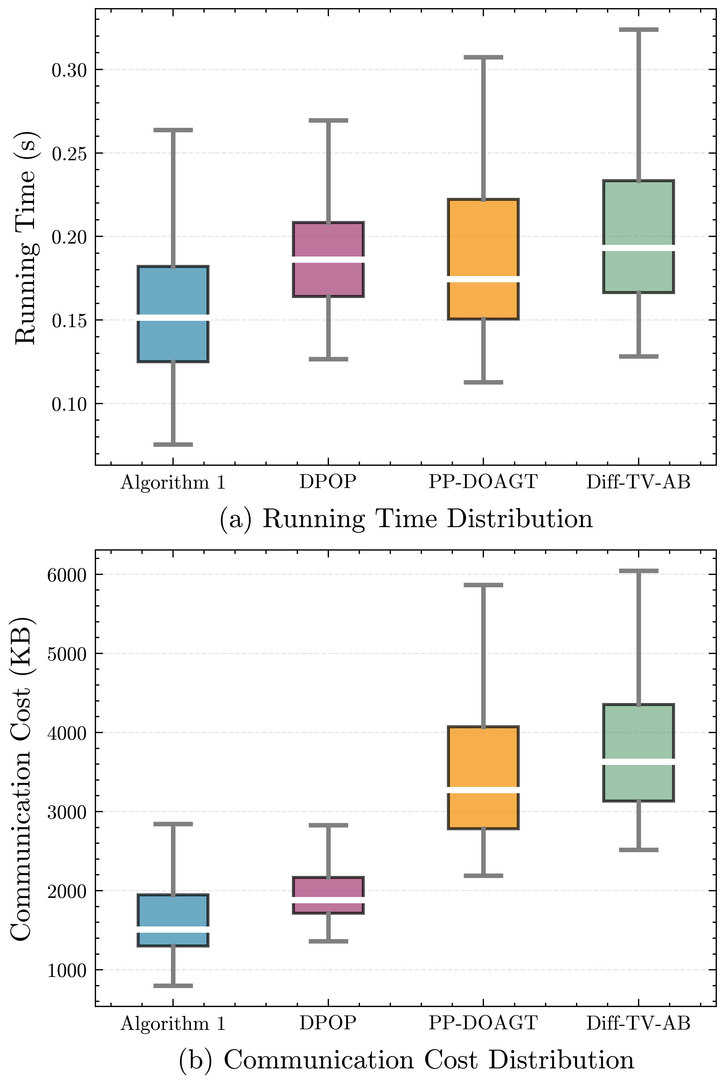
Fig. 5: Running time and communication cost comparison of different algorithms.

To further validate the practical efficiency of Algorithm 1, we conduct a comparative experiment among four methods: Algorithm 1, DPOP, PP-DOAGT, and Diff-TV-AB under identical problem configurations. We adopt the same stopping criterion, that is, the iteration is terminated when the optimization residual falls below 1×10⁻²¹\times 10^{-2}. To ensure statistical reliability, we perform 100 valid independent runs for each method and record the running time and total communication cost for every trial. The results are presented in Fig. 5. Algorithm 1 achieves the lowest median running time and the smallest median communication cost, demonstrating significantly better performance than PP-DOAGT and Diff-TV-AB. This advantage can be attributed to two main factors. On one hand, compared with DPOP, Algorithm 1 exhibits better convergence behavior, reaching the prescribed accuracy in fewer iterations. On the other hand, relative to PP-DOAGT and Diff-TV-AB, Algorithm 1 significantly reduces the per-iteration computational and communication overhead (see Table II), which yields higher efficiency in each iteration step.

VI-B Comparison of Differentially Private Methods Based on Distributed Learning on MNIST

In this subsection, we further validate the effectiveness of Algorithm 1 through distributed learning tasks on the MNIST dataset, while comprehensively evaluating its performance via parameter sensitivity analysis and privacy-accuracy trade-off studies. The MNIST dataset, a classic benchmark comprising handwritten digit images, is widely utilized for evaluating algorithm performance in image classification tasks. In this experiment, we consider a distributed learning scenario with 100 agents collaboratively training a convolutional neural network (CNN), whose communication topology is illustrated in Fig. 1. The CNN architecture adopts a two-layer convolutional structure: each layer consists of a 5×55\times 5 convolution, BatchNorm normalization, and a 2×22\times 2 max-pooling operation, followed by a fully-connected layer that outputs predictions over 10 classes. Each agent maintains a local copy of this CNN. We uniformly distribute the MNIST training images across all agents and train the model using a batch size of 16 with a cross-entropy loss function.

Refer to caption
Fig. 6: Accuracy comparison between Algorithm 1 and DPOP [18] under the same privacy budget on MNIST image classification.
Refer to caption
Fig. 7: Accuracy comparison between Algorithm 1 and PP-DOAGT [24] under the same noise on MNIST image classification.
Refer to caption
Fig. 8: Accuracy comparison between Algorithm 1 and Diff-TV-AB [21] under the same noise on MNIST image classification.

For Algorithm 1, the relevant parameters are set as γ=0.001\gamma=0.001, β=100\beta=100, q2=0.999q_{2}=0.999, and q1=0.998q_{1}=0.998. We record the evolution of training and testing accuracy of Algorithm 1 under a privacy budget of ϵ=1\epsilon=1, as shown by the blue lines in Fig. 6. The results demonstrate that the final training and testing accuracy both exceed 90%, indicating that our algorithm can maintain high model performance while ensuring DP. For comparison, we implement the DPOP method from [18], with its performance depicted by the orange lines in Fig. 6. Under the same privacy budget, our algorithm demonstrates superior performance in both training and testing accuracy compared to the DPOP method. Furthermore, we reproduce two recently proposed methods, PP-DOAGT [24] and Diff-TV-AB [21], with experimental results shown by the orange lines in Figs. 7 and 8. The results indicate that under the same noise conditions, our algorithm achieves optimization accuracy comparable to both PP-DOAGT and Diff-TV-AB. Benefiting from its lower sensitivity design (as shown in Table III), our algorithm exhibits stronger privacy protection performance relative to PP-DOAGT and Diff-TV-AB.

Refer to caption
Fig. 9: Testing accuracy of Algorithm 1 under different γ\gamma and β\beta parameter configurations.

To evaluate the robustness and stability of Algorithm 1, we conduct a parameter sensitivity analysis, focusing on the effects of initial stepsize parameter γ\gamma and parameter β\beta on model performance. The parameter γ\gamma is tested over the range {0.001,0.005,0.01,0.05,0.1}\{0.001,0.005,0.01,0.05,0.1\}, while β\beta is evaluated across {0.1,1,10,100,1000}\{0.1,1,10,100,1000\}. Experimental results using testing accuracy as the evaluation metric are presented in Fig. 9. Analysis reveals that when γ\gamma takes relatively small values (specifically γ≤0.01\gamma\leq 0.01), and β\beta satisfies γ​β≤1\gamma\beta\leq 1, the algorithm achieves stable testing accuracy exceeding 85%, demonstrating desirable performance levels. This finding experimentally validates the necessity of the condition γ​β≤1\gamma\beta\leq 1 for convergence. Furthermore, we observe that within the range of γ≤0.01\gamma\leq 0.01, even with substantial variations in β\beta values, testing accuracy remains consistently high as long as γ​β≤1\gamma\beta\leq 1 is maintained. This indicates Algorithm 1’s insensitivity to parameter variations and confirms its strong robustness.

Refer to caption
Fig. 10: Privacy-accuracy trade-off of Algorithm 1 under different network topologies and scales.

To further evaluate the performance of Algorithm 1, we systematically investigate its privacy-accuracy trade-off characteristics under different network topologies (ring graph and ER random graph) and network scales (n=50n=50 and n=100n=100). The experimental results are presented in Fig. 10. Analysis of Fig. 10 reveals that across all experimental configurations, testing accuracy consistently improves with increasing the privacy budget ϵ\epsilon, clearly demonstrating the inherent privacy-accuracy trade-off in differentially private algorithms, which aligns with the theoretical result in Theorem 2. Furthermore, under the same privacy budgets, the ER random graph topology achieves higher testing accuracy compared to the ring graph topology. This phenomenon can be attributed to the higher connectivity of random graphs, which facilitates information propagation among agents, thereby accelerating convergence and enhancing final performance. Notably, across all combinations of network topologies and scales, Algorithm 1 maintains testing accuracy above 85% when the privacy budget ϵ≥0.5\epsilon\geq 0.5. These results demonstrate both the scalability of Algorithm 1 and its capability to maintain high model accuracy while providing moderate privacy protection.

Refer to caption
Fig. 11: Schematic illustration of the honest-but-curious adversary and the external eavesdropper.
TABLE IV: Comparison of the Privacy, Accuracy, Applicability, and Efficiency of the Three Different Types of Algorithms.
Methods M-NMI under M-NMI under Accuracy Topological Efficiency
external eavesdropper honest-but-curious adversary assumption
Algorithm 1 with ϵ=10\epsilon=10 0.52 0.52 1.9×10−41.9\times 10^{-4} ✗ High
Algorithm 1 with ϵ=1\epsilon=1 0.24 0.24 2.0×10−32.0\times 10^{-3} ✗ High
Algorithm 1 with ϵ=0.1\epsilon=0.1 0.047 0.047 3.0×10−23.0\times 10^{-2} ✗ High
Correlated randomness-based method [8] 1 0.47 6.6×10−96.6\times 10^{-9} ✓ High
Encryption-based method [12] 0 0.30 3.2×10−63.2\times 10^{-6} ✗ Low

VI-C Comprehensive Performance Comparison Across Different Types of Privacy-Preserving Methods

To objectively evaluate the privacy levels of different types of privacy-preserving algorithms, we employ the Maximum Normalized Mutual Information (M-NMI), a modified mutual information-based metric from [36], as the privacy measure:

M-NMI≜max1≤k≤K⁡{I⁡(𝒱i​(k),ℐj​(k))I⁡(𝒱i​(k),𝒱i​(k))},\displaystyle\text{M-NMI}\triangleq\max_{1\leq k\leq K}\left\{\frac{I(\mathcal{V}_{i}(k),\mathcal{I}_{j}(k))}{I(\mathcal{V}_{i}(k),\mathcal{V}_{i}(k))}\right\}, (43)

where 𝒱i​(k)\mathcal{V}_{i}(k) is the private variable of agent ii at iteration kk, ℐj​(k)\mathcal{I}_{j}(k) represent the information attacker jj can obtain about 𝒱i​(k)\mathcal{V}_{i}(k), and KK is the total number of iterations. I⁡(𝒱i​(k),ℐj​(k))I(\mathcal{V}_{i}(k),\mathcal{I}_{j}(k)) is the mutual information between 𝒱i​(k)\mathcal{V}_{i}(k) and ℐj​(k)\mathcal{I}_{j}(k), which quantifies the amount of agent ii’s private information contained in the information acquired by attacker jj. I⁡(𝒱i​(k),𝒱i​(k))I(\mathcal{V}_{i}(k),\mathcal{V}_{i}(k)) represents the entropy of agent ii’s private information, which is used for normalization. M-NMI quantifies the worst-case privacy leakage across all iterations. A smaller M-NMI value indicates stronger privacy preservation of the algorithm. For 𝒱i​(k)\mathcal{V}_{i}(k), we consider the agent’s gradients as its private information [2]. For ℐj​(k)\mathcal{I}_{j}(k), it depends on the attacker’s model and the algorithm’s update rule. We consider two common attacker models: the honest-but-curious adversary and the external eavesdropper [37]. We adopt the system as shown in Fig. 11, in which agent 1 is an honest agent, agents 2 and 3 are honest-but-curious adversaries, and agent ee is an external eavesdropper. Agents 1, 2, and 3 collaboratively solve Problem (42) with dimensions m=1m=1 and p=1p=1. Agents 2, 3, and ee all attempt to infer the private information of agent 1. For each method, we perform 5,000 Monte Carlo trials, each comprising 1,000 iterations. We then compute its M-NMI values under the honest-but-curious adversary and the external eavesdropper using the NPEET toolbox [38].

Under Algorithm 1, the private information of agent 1 is ∇f1​(𝒛1​(k)),1≤k≤K\nabla f_{1}\left(\bm{z}_{1}(k)\right),1\leq k\leq K, i.e., 𝒱1​(k)={∇f1​(𝒛1​(k))}\mathcal{V}_{1}(k)=\left\{\nabla f_{1}\left(\bm{z}_{1}(k)\right)\right\}. Honest-but-curious adversaries 2 and 3 can collude to infer the private information of agent 1. They receive 𝒛1​(k)\bm{z}_{1}(k) from agent 1, infer 𝒚1​(k)\bm{y}_{1}(k) using update (4b) and public information WW and β\beta, and approximate ∇f1​(𝒛1​(k))\nabla f_{1}\left(\bm{z}_{1}(k)\right) using update (4c) and public information αk\alpha_{k}, that is,

ℐ2​(k)={𝒛1​(k),𝒚1​(k),1αk​(𝒛¯1​(k)−𝒛1​(k))−𝒚1​(k)}.\displaystyle\mathcal{I}_{2}(k)=\left\{\bm{z}_{1}(k),\bm{y}_{1}(k),\frac{1}{\alpha_{k}}\left(\bar{\bm{z}}_{1}(k)-\bm{z}_{1}(k)\right)-\bm{y}_{1}(k)\right\}. (44)

The external eavesdropper ee acquires the same information about agent 1 as the honest-but-curious adversaries, leading to ℐ​e​(k)=ℐ2​(k)\mathcal{I}{e}(k)=\mathcal{I}_{2}(k). The corresponding simulation results under different privacy budgets are shown in the first three rows of Table IV. It can be seen that our algorithm can simultaneously defend against the honest-but-curious adversary and the external eavesdropper. Furthermore, as the privacy budget decreases, both the M-NMI value and optimization accuracy decline, which aligns with the intuition of a differentially private algorithm.

For comparison, we implement the correlated randomness-based privacy-preserving method from [8]. The correlated randomness-based method relies on an additional topological assumption: each honest agent has at least one neighboring agent that is also honest. Thus, for this method, we assume that agent 3 in Fig. 11 is also an honest agent, and we compute its M-NMI under the honest-but-curious adversary using the following information:

ℐ2​(k)={𝒙1k,Λ1k​𝒚1k,C21k​𝒚1k+B21k​(∇f1​(𝒙1k+1)−∇f1​(𝒙1k))},\displaystyle\mathcal{I}_{2}(k)=\left\{\bm{x}_{1}^{k},\Lambda_{1}^{k}\bm{y}_{1}^{k},C_{21}^{k}\bm{y}_{1}^{k}+B_{21}^{k}(\nabla f_{1}(\bm{x}_{1}^{k+1})-\nabla f_{1}(\bm{x}_{1}^{k}))\right\},

which consists of information directly received by agent 2 from agent 1. The relevant results are shown in the fourth row of Table IV. It can be observed that this method achieves high accuracy, as the correlated randomness-based method enables exact convergence. Under the external eavesdropper, the M-NMI value of this method is 1, indicating that it cannot defend against the external eavesdropper. This is because the privacy of the correlated randomness-based method relies on the additional topological assumption, which does not work against the external eavesdropper. We also implement the encryption-based privacy-preserving method from [12]. Its M-NMI under the honest-but-curious adversary is computed using the following information:

ℐ2(k)={1αk(∑j∈{2,3}b1→jbj→1(𝒙j(k)−𝒙1(k))},\displaystyle\mathcal{I}_{2}(k)=\Big\{\frac{1}{\alpha_{k}}\Big(\sum_{j\in\{2,3\}}b_{1\to j}b_{j\to 1}(\bm{x}_{j}(k)-\bm{x}_{1}(k)\Big)\Big\},

which is an estimate of agent 1’s gradient according to its update rule. The corresponding results are shown in the last row of Table IV. It can be seen that this method achieves an M-NMI value of 0 under the external eavesdropper, meaning the encryption-based method is fully resistant to the external eavesdropper. This is because the external eavesdropper can only access encrypted data. Moreover, this method exhibits high accuracy as the encryption-based method can also achieve exact convergence. However, the encryption-based method requires numerous encryption and decryption operations, resulting in low computational and communication efficiency. In addition, although all three types of algorithms can defend against the honest-but-curious adversary, Table IV demonstrates that our algorithm allows for enhanced privacy performance through adjustable privacy budgets, whereas the privacy performance of the other two methods remains fixed.

Based on the comparative results presented in Table IV, the proposed algorithm demonstrates distinct advantages in the following practical deployment scenarios:

  1. 1.

    Scenarios Requiring Defense Against Both Internal and External Threats: Correlated randomness-based methods fail to protect against external eavesdroppers (M‑NMI = 1). The proposed algorithm achieves low M‑NMI values under the external eavesdropper and honest-but-curious adversary, confirming its capability to resist both types of adversaries simultaneously.

  2. 2.

    Scenarios Demanding Tunable and Quantifiable Privacy Guarantees: Both correlated randomness-based and encryption-based methods offer a fixed level of privacy protection. Our algorithm allows the privacy budget ϵ\epsilon to be adjusted according to specific application requirements, providing configurable and provable privacy.

  3. 3.

    Resource-Constrained Large-Scale Distributed Systems: Encryption-based methods incur high computational and communication overhead due to frequent encryption and decryption operations. The proposed algorithm only requires lightweight noise injection and, compared to existing DP gradient-tracking methods, reduces the number of communication variables and noise injections by half, significantly lowering the resource burden.

  4. 4.

    Networks with Dynamic or Unknown Topology: Correlated randomness-based methods rely on the assumption that each honest agent has at least one honest neighbor, which is often impractical in self-organizing or time-varying networks. Our algorithm only requires network connectivity, making it directly applicable to mobile or peer-to-peer networks without imposing additional topological constraints.

In summary, the proposed differentially private algorithm provides a versatile and practical solution for privacy-preserving distributed optimization. It effectively balances provable privacy, a configurable privacy-accuracy trade-off, lower resource overhead, and broader topological applicability under various real-world constraints and threat models.

VII Conclusion

In this paper, we propose a differentially private distributed optimization algorithm for undirected graphs, and derive an explicit closed-form expression for the noise parameter as a function of the privacy budget. Compared to existing state-of-the-art algorithms, the proposed algorithm exhibits lower sensitivity, thereby achieving higher optimization accuracy under the same privacy budget. Furthermore, the proposed algorithm reduces both the number of communication variables and the amount of injected noise by half, significantly enhancing communication and computational efficiency. Moreover, we rigorously analyze the algorithm’s differential privacy, establish its convergence, and derive an upper bound on its optimization accuracy. The theoretical results reveal the inherent trade-off between privacy and accuracy and provide guidance for parameter tuning. Future work will proceed along three promising directions: (i) Extending the sensitivity‑reduction framework to directed graph topologies. (ii) Enhancing the algorithm’s convergence rate while preserving its privacy and accuracy guarantees, where potential pathways include designing adaptive stepsize schedules (e.g., two-phase or noise-aware decay) and incorporating variance‑reduction techniques. (iii) Generalizing the algorithm to broader problem classes, including convex (but not strongly convex) objectives and structured nonconvex problems frequently encountered in modern machine learning.

Appendix A Proof of Proposition 1

Proof:

We prove the proposition by directly comparing the algorithm’s sensitivity under different designs. We consider the classical differentially private distributed gradient descent (DP-DGD) as the baseline algorithm:

𝐱(k)=W𝐳(k)−αk∇F(𝐳(k)),\mathbf{x}(k)=W\mathbf{z}(k)-\alpha_{k}\nabla F(\mathbf{z}(k)), (45)

where 𝐳⁡(k)≜𝐱⁡(k−1)+𝝃⁡(k)\mathbf{z}(k)\triangleq\mathbf{x}(k-1)+\bm{\xi}(k) is the noisy state and αk\alpha_{k} is the stepsize. Note that in the DP-DGD algorithm, agents use their own noisy states for consensus and compute gradients based on noisy states. According to Definition 3, and since

‖𝐱⁡(k)−𝐱′​(k)‖1\displaystyle\|\mathbf{x}(k)-\mathbf{x}^{\prime}(k)\|_{1} =‖𝒙i0​(k)−𝒙i0′​(k)‖1\displaystyle=\|\bm{x}_{i_{0}}(k)-\bm{x}_{i_{0}}^{\prime}(k)\|_{1} (46)
=αk​‖∇fi0​(𝒛i0​(k))−∇fi0′​(𝒛i0​(k))‖1\displaystyle=\alpha_{k}\|\nabla f_{i_{0}}(\bm{z}_{i_{0}}(k))-\nabla f_{i_{0}}^{\prime}(\bm{z}_{i_{0}}(k))\|_{1}
≤δ​αk,\displaystyle\leq\delta\alpha_{k},

the sensitivity of the DP-DGD algorithm, denoted as Δ1​(k)\Delta_{1}(k), is bounded by δ​αk\delta\alpha_{k}, i.e., Δ1​(k)≤δ​αk\Delta_{1}(k)\leq\delta\alpha_{k}. The proof details for (46) can be found in Theorem 1 or in Lemma 4 of [18].

If agents use their true states for consensus, the DP-DGD algorithm can be reformulated as

𝐱(k)=W0𝐱(k−1)+(W−W0)𝐳(k)−αk∇F(𝐳(k)),\mathbf{x}(k)=W_{0}\mathbf{x}(k-1)+(W-W_{0})\mathbf{z}(k)-\alpha_{k}\nabla F(\mathbf{z}(k)), (47)

where W0≜diag​{W}W_{0}\triangleq\text{diag}\{W\}. Let Δ2​(k)\Delta_{2}(k) denote the sensitivity of the above algorithm at iteration kk. Since ‖𝒙i0​(k)−𝒙i0′​(k)‖1=‖Wi0​i0​(𝒙i0​(k−1)−𝒙i0′​(k−1))−αk​(∇fi0​(𝒛i0​(k))−∇fi0′​(𝒛i0​(k)))‖1≤Wi0​i0​Δ2​(k−1)+δ​αk\|\bm{x}_{i_{0}}(k)-\bm{x}_{i_{0}}^{\prime}(k)\|_{1}=\|W_{i_{0}i_{0}}(\bm{x}_{i_{0}}(k-1)-\bm{x}_{i_{0}}^{\prime}(k-1))-\alpha_{k}(\nabla f_{i_{0}}(\bm{z}_{i_{0}}(k))-\nabla f_{i_{0}}^{\prime}(\bm{z}_{i_{0}}(k)))\|_{1}\leq W_{i_{0}i_{0}}\Delta_{2}(k-1)+\delta\alpha_{k}, we have Δ2​(k)≤Wi0​i0​Δ2​(k−1)+δ​αk\Delta_{2}(k)\leq W_{i_{0}i_{0}}\Delta_{2}(k-1)+\delta\alpha_{k}. Due to Δ2​(k−1)≥0\Delta_{2}(k-1)\geq 0 for all k≥1k\geq 1, we obtain the first argument.

If agents compute gradients based on their true states, the DP-DGD algorithm is reformulated as

𝐱(k)=W𝐳(k)−αk∇F(𝐱(k−1)).\mathbf{x}(k)=W\mathbf{z}(k)-\alpha_{k}\nabla F(\mathbf{x}(k-1)). (48)

Let Δ3​(k)\Delta_{3}(k) denote the sensitivity of the above algorithm at iteration kk. Since ‖𝒙i0​(k)−𝒙i0′​(k)‖1=αk​‖∇fi0​(𝒙i0​(k−1))−∇fi0′​(𝒙i0′​(k−1))‖1=αk​‖∇fi0​(𝒙i0​(k−1))−∇fi0​(𝒙i0′​(k−1))+∇fi0​(𝒙i0′​(k−1))−∇fi0′​(𝒙i0′​(k−1))‖1≤n​L​αk​Δ3​(k−1)+δ​αk\|\bm{x}_{i_{0}}(k)-\bm{x}_{i_{0}}^{\prime}(k)\|_{1}=\alpha_{k}\|\nabla f_{i_{0}}(\bm{x}_{i_{0}}(k-1))-\nabla f_{i_{0}}^{\prime}(\bm{x}_{i_{0}}^{\prime}(k-1))\|_{1}=\alpha_{k}\|\nabla f_{i_{0}}(\bm{x}_{i_{0}}(k-1))-\nabla f_{i_{0}}(\bm{x}_{i_{0}}^{\prime}(k-1))+\nabla f_{i_{0}}(\bm{x}_{i_{0}}^{\prime}(k-1))-\nabla f_{i_{0}}^{\prime}(\bm{x}_{i_{0}}^{\prime}(k-1))\|_{1}\leq\sqrt{n}L\alpha_{k}\Delta_{3}(k-1)+\delta\alpha_{k}, we obtain Δ3​(k)≤n​L​αk​Δ3​(k−1)+δ​αk\Delta_{3}(k)\leq\sqrt{n}L\alpha_{k}\Delta_{3}(k-1)+\delta\alpha_{k}. Because of Δ3​(k−1)≥0\Delta_{3}(k-1)\geq 0 for all k≥1k\geq 1, we have the second argument.

For the third argument, when neighboring agents share only variable 𝒙\bm{x}, the algorithm’s sensitivity depends on the bound of ‖𝐱⁡(k)−𝐱′​(k)‖1\|\mathbf{x}(k)-\mathbf{x}^{\prime}(k)\|_{1}. If agents are also required to exchange additional variables (e.g., an auxiliary variable 𝒚\bm{y}), the algorithm’s sensitivity increases to ‖𝐱⁡(k)−𝐱′​(k)‖1+‖𝐲⁡(k)−𝐲′​(k)‖1\|\mathbf{x}(k)-\mathbf{x}^{\prime}(k)\|_{1}+\|\mathbf{y}(k)-\mathbf{y}^{\prime}(k)\|_{1}. Hence, the third argument holds. ∎

Appendix B Proof of Basic Lemmas

B-A Proof of Lemma 3

Proof:

It follows from Assumption 3 that 𝔼⁡[𝝃⁡(k)|ℳk]=0\mathbb{E}\left[\bm{\xi}(k)|\mathcal{M}_{k}\right]=0, 𝔼⁡[‖𝝃⁡(k)‖|ℳk]≤n​p​νk\mathbb{E}\left[\|\bm{\xi}(k)\||\mathcal{M}_{k}\right]\leq np\nu_{k}, and 𝔼⁡[‖𝝃⁡(k)‖2|ℳk]=2​n​p​νk2\mathbb{E}\left[\|\bm{\xi}(k)\|^{2}|\mathcal{M}_{k}\right]=2np\nu_{k}^{2}. For part (a), it follows from the definition of 𝐳⁡(k)\mathbf{z}(k) that

𝔼⁡[⟨𝐳⁡(k),𝝃⁡(k)⟩|ℳk]\displaystyle\mathbb{E}\left[\langle\mathbf{z}(k),\bm{\xi}(k)\rangle|\mathcal{M}_{k}\right] =𝔼⁡[⟨𝝃⁡(k),𝝃⁡(k)⟩|ℳk]\displaystyle=\mathbb{E}\left[\langle\bm{\xi}(k),\bm{\xi}(k)\rangle|\mathcal{M}_{k}\right] (49)
≤𝔼⁡[‖𝝃⁡(k)‖2|ℳk]\displaystyle\leq\mathbb{E}\left[\|\bm{\xi}(k)\|^{2}|\mathcal{M}_{k}\right]
=2​n​p​νk2.\displaystyle=2np\nu_{k}^{2}.

For part (b), in light of Assumption 1, we have

𝔼⁡[⟨∇F​(𝐳⁡(k)),𝝃⁡(k)⟩|ℳk]\displaystyle\mathbb{E}\left[\left\langle\nabla F(\mathbf{z}(k)),\bm{\xi}(k)\right\rangle|\mathcal{M}_{k}\right] (50)
=𝔼⁡[⟨∇F​(𝐳⁡(k))−∇F​(𝐱⁡(k−1)),𝝃⁡(k)⟩|ℳk]\displaystyle=\mathbb{E}\left[\left\langle\nabla F(\mathbf{z}(k))-\nabla F(\mathbf{x}(k-1)),\bm{\xi}(k)\right\rangle|\mathcal{M}_{k}\right]
≤L​𝔼​[‖𝝃⁡(k)‖2|ℳk]\displaystyle\leq L\mathbb{E}\left[\|\bm{\xi}(k)\|^{2}|\mathcal{M}_{k}\right]
=2​n​p​L​νk2.\displaystyle=2npL\nu_{k}^{2}.

For part (c), following a similar derivation as in Lemma 8 of [34], we obtain

𝔼⁡[⟨∇F​(𝐱⁡(k)),𝝃⁡(k)⟩|ℳk]\displaystyle\mathbb{E}\left[\left\langle\nabla F(\mathbf{x}(k)),\bm{\xi}(k)\right\rangle|\mathcal{M}_{k}\right] (51)
≤∑i=1n(L​|Wi​i−αk​β+αk​β​Wi​i|+L2​αk)​𝔼​[‖𝝃i​(k)‖2|ℳk]\displaystyle\leq\sum_{i=1}^{n}\left(L|W_{ii}-\alpha_{k}\beta+\alpha_{k}\beta W_{ii}|+L^{2}\alpha_{k}\right)\mathbb{E}\left[\|\bm{\xi}_{i}(k)\|^{2}|\mathcal{M}_{k}\right]
≤2​n​p​(L+L2​αk)​νk2,\displaystyle\leq 2np(L+L^{2}\alpha_{k})\nu_{k}^{2},

where the second inequality follows from the fact that Wi​i−αk​β+αk​β​Wi​i∈(−1,1)W_{ii}-\alpha_{k}\beta+\alpha_{k}\beta W_{ii}\in(-1,1). Then, we have

𝔼⁡[⟨∇F​(𝐳⁡(k+1)),𝝃⁡(k)⟩|ℳk]\displaystyle\mathbb{E}\left[\left\langle\nabla F(\mathbf{z}(k+1)),\bm{\xi}(k)\right\rangle|\mathcal{M}_{k}\right] (52)
=𝔼⁡[⟨∇F​(𝐳⁡(k+1))−∇F​(𝐱⁡(k)),𝝃⁡(k)⟩|ℳk]\displaystyle=\mathbb{E}\left[\left\langle\nabla F(\mathbf{z}(k+1))-\nabla F(\mathbf{x}(k)),\bm{\xi}(k)\right\rangle|\mathcal{M}_{k}\right]
+𝔼⁡[⟨∇F​(𝐱⁡(k)),𝝃⁡(k)⟩|ℳk]\displaystyle+\mathbb{E}\left[\left\langle\nabla F(\mathbf{x}(k)),\bm{\xi}(k)\right\rangle|\mathcal{M}_{k}\right]
≤L​𝔼​[‖𝝃⁡(k+1)‖​‖𝝃⁡(k)‖|ℳk]+2​n​p​(L+L2​αk)​νk2\displaystyle\leq L\mathbb{E}\left[\|\bm{\xi}(k+1)\|\|\bm{\xi}(k)\||\mathcal{M}_{k}\right]+2np(L+L^{2}\alpha_{k})\nu_{k}^{2}
≤n2​p2​L​νk+1​νk+2​n​p​(L+L2​αk)​νk2\displaystyle\leq n^{2}p^{2}L\nu_{k+1}\nu_{k}+2np(L+L^{2}\alpha_{k})\nu_{k}^{2}
≤n​p​L​(2+n​p+2​L​αk)​νk2.\displaystyle\leq npL(2+np+2L\alpha_{k})\nu_{k}^{2}.

For part (d), by substituting (13a) into (13b), we get

𝐱⁡(k)\displaystyle\mathbf{x}(k) =((1+αk​β)​W−αk​β​I)​𝐳​(k)−αk​𝐲​(k−1)\displaystyle=((1+\alpha_{k}\beta)W-\alpha_{k}\beta I)\mathbf{z}(k)-\alpha_{k}\mathbf{y}(k-1) (53)
−αk∇F(𝐳(k)).\displaystyle-\alpha_{k}\nabla F(\mathbf{z}(k)).

Since 𝐲⁡(k−1)\mathbf{y}(k-1) is uniquely determined by ℳk\mathcal{M}_{k}, and based on parts (a) and (b), we have

𝔼⁡[⟨𝐱⁡(k),𝝃⁡(k)⟩|ℳk]\displaystyle\mathbb{E}\left[\langle\mathbf{x}(k),\bm{\xi}(k)\rangle|\mathcal{M}_{k}\right] (54)
=𝔼[⟨((1+αkβ)W−αkβI)𝐳(k)−αk∇F(𝐳(k)),𝝃(k)⟩|ℳk]\displaystyle=\mathbb{E}\left[\left\langle((1+\alpha_{k}\beta)W-\alpha_{k}\beta I)\mathbf{z}(k)-\alpha_{k}\nabla F(\mathbf{z}(k)),\bm{\xi}(k)\right\rangle|\mathcal{M}_{k}\right]
≤2​n​p​(‖(1+αk​β)​W−αk​β​I‖+L​αk)​νk2\displaystyle\leq 2np\left(\|(1+\alpha_{k}\beta)W-\alpha_{k}\beta I\|+L\alpha_{k}\right)\nu_{k}^{2}
≤2​n​p​(3+L​αk)​νk2.\displaystyle\leq 2np\left(3+L\alpha_{k}\right)\nu_{k}^{2}.

For part (e), it follows from (14) and parts (a) and (b) that

𝔼⁡[⟨𝟏​𝒙¯​(k),𝝃⁡(k)⟩|ℳk]\displaystyle\mathbb{E}\left[\langle\mathbf{1}\bar{\bm{x}}(k),\bm{\xi}(k)\rangle|\mathcal{M}_{k}\right] (55)
=𝔼[⟨1n𝟏𝟏T𝐳(k)−αkn𝟏𝟏T∇F(𝐳(k)),𝝃(k)⟩|ℳk]\displaystyle=\mathbb{E}\left[\left\langle\frac{1}{n}\mathbf{1}\mathbf{1}^{T}\mathbf{z}(k)-\frac{\alpha_{k}}{n}\mathbf{1}\mathbf{1}^{T}\nabla F(\mathbf{z}(k)),\bm{\xi}(k)\right\rangle|\mathcal{M}_{k}\right]
≤2​n​p​(1+L​αk)​νk2.\displaystyle\leq 2np(1+L\alpha_{k})\nu_{k}^{2}.

By the definition of 𝐳⁡(k)\mathbf{z}(k), part (f) can be obtained as follows:

𝔼⁡[‖𝐳⁡(k+1)−𝟏​𝒙¯​(k)‖2|ℳk]\displaystyle\mathbb{E}\left[\|\mathbf{z}(k+1)-\mathbf{1}\bar{\bm{x}}(k)\|^{2}|\mathcal{M}_{k}\right] (56)
=𝔼⁡[‖𝐱⁡(k)−𝟏​𝒙¯​(k)+𝝃⁡(k+1)‖2|ℳk]\displaystyle=\mathbb{E}\left[\|\mathbf{x}(k)-\mathbf{1}\bar{\bm{x}}(k)+\bm{\xi}(k+1)\|^{2}|\mathcal{M}_{k}\right]
=𝔼⁡[‖𝐱⁡(k)−𝟏​𝒙¯​(k)‖2|ℳk]+𝔼⁡[‖𝝃⁡(k+1)‖2|ℳk]\displaystyle=\mathbb{E}\left[\|\mathbf{x}(k)-\mathbf{1}\bar{\bm{x}}(k)\|^{2}|\mathcal{M}_{k}\right]+\mathbb{E}\left[\|\bm{\xi}(k+1)\|^{2}|\mathcal{M}_{k}\right]
=𝔼⁡[‖𝐱⁡(k)−𝟏​𝒙¯​(k)‖2|ℳk]+2​n​p​νk+12.\displaystyle=\mathbb{E}\left[\|\mathbf{x}(k)-\mathbf{1}\bar{\bm{x}}(k)\|^{2}|\mathcal{M}_{k}\right]+2np\nu_{k+1}^{2}.

Similarly, we have

𝔼⁡[‖𝐳⁡(k+1)−𝐳⁡(k)‖2|ℳk]\displaystyle\mathbb{E}\left[\|\mathbf{z}(k+1)-\mathbf{z}(k)\|^{2}|\mathcal{M}_{k}\right] (57)
=𝔼⁡[‖𝐱⁡(k)−𝐱⁡(k−1)+𝝃⁡(k+1)−𝝃⁡(k)‖2|ℳk]\displaystyle=\mathbb{E}\left[\|\mathbf{x}(k)-\mathbf{x}(k-1)+\bm{\xi}(k+1)-\bm{\xi}(k)\|^{2}|\mathcal{M}_{k}\right]
=𝔼⁡[‖𝐱⁡(k)−𝐱⁡(k−1)‖2|ℳk]+𝔼⁡[‖𝝃⁡(k+1)−𝝃⁡(k)‖2|ℳk]\displaystyle=\mathbb{E}\left[\|\mathbf{x}(k)-\mathbf{x}(k-1)\|^{2}|\mathcal{M}_{k}\right]+\mathbb{E}\left[\|\bm{\xi}(k+1)-\bm{\xi}(k)\|^{2}|\mathcal{M}_{k}\right]
+2​𝔼​[⟨𝐱⁡(k),−𝝃⁡(k)⟩|ℳk]\displaystyle+2\mathbb{E}\left[\langle\mathbf{x}(k),-\bm{\xi}(k)\rangle|\mathcal{M}_{k}\right]
≤𝔼⁡[‖𝐱⁡(k)−𝐱⁡(k−1)‖2|ℳk]+2​n​p​νk+12\displaystyle\leq\mathbb{E}\left[\|\mathbf{x}(k)-\mathbf{x}(k-1)\|^{2}|\mathcal{M}_{k}\right]+2np\nu_{k+1}^{2}
+2​n​p​(7+2​L​αk)​νk2,\displaystyle+2np(7+2L\alpha_{k})\nu_{k}^{2},

where in the first inequality we use part (d). ∎

B-B Proof of Lemma 5

Proof:

Let 𝒂1≜𝒙¯(k)−αk+1n𝟏T∇F(𝟏𝒙¯(k))−𝒙∗\bm{a}_{1}\triangleq\bar{\bm{x}}(k)-\frac{\alpha_{k+1}}{n}\mathbf{1}^{T}\nabla F(\mathbf{1}\bar{\bm{x}}(k))-\bm{x}^{*}, 𝒃1≜αk+1n​𝟏T​(∇F​(𝐳⁡(k+1))−∇F​(𝟏​𝒙¯​(k)))\bm{b}_{1}\triangleq\frac{\alpha_{k+1}}{n}\mathbf{1}^{T}\left(\nabla F(\mathbf{z}(k+1))-\nabla F(\mathbf{1}\bar{\bm{x}}(k))\right), and 𝒄1≜1n​𝟏T​𝝃​(k+1)\bm{c}_{1}\triangleq\frac{1}{n}\mathbf{1}^{T}\bm{\xi}(k+1). In light of (15) and Lemma 2, if αk+1≤2μ+L\alpha_{k+1}\leq\frac{2}{\mu+L} for any k≥0k\geq 0, we have

𝔼⁡[‖𝒙¯​(k+1)−𝒙∗‖2|ℳk]\displaystyle\mathbb{E}\left[\|\bar{\bm{x}}(k+1)-\bm{x}^{*}\|^{2}|\mathcal{M}_{k}\right] (58)
=𝔼⁡[‖𝒂1‖2|ℳk]+𝔼⁡[‖𝒃1‖2|ℳk]+𝔼⁡[‖𝒄1‖2|ℳk]\displaystyle=\mathbb{E}\left[\|\bm{a}_{1}\|^{2}|\mathcal{M}_{k}\right]+\mathbb{E}\left[\|\bm{b}_{1}\|^{2}|\mathcal{M}_{k}\right]+\mathbb{E}\left[\|\bm{c}_{1}\|^{2}|\mathcal{M}_{k}\right]
+𝔼⁡[2​⟨𝒂1,−𝒃1⟩|ℳk]+𝔼⁡[2​⟨−𝒃1,𝒄1⟩|ℳk]\displaystyle+\mathbb{E}\left[2\langle\bm{a}_{1},-\bm{b}_{1}\rangle|\mathcal{M}_{k}\right]+\mathbb{E}\left[2\langle-\bm{b}_{1},\bm{c}_{1}\rangle|\mathcal{M}_{k}\right]
≤(1−αk+1​μ)2​𝔼​[‖𝒙¯​(k)−𝒙∗‖2|ℳk]\displaystyle\leq(1-\alpha_{k+1}\mu)^{2}\mathbb{E}\left[\|\bar{\bm{x}}(k)-\bm{x}^{*}\|^{2}|\mathcal{M}_{k}\right]
+L2​αk+12n​𝔼​[‖𝐳⁡(k+1)−𝟏​𝒙¯​(k)‖2|ℳk]\displaystyle+\frac{L^{2}\alpha_{k+1}^{2}}{n}\mathbb{E}\left[\|\mathbf{z}(k+1)-\mathbf{1}\bar{\bm{x}}(k)\|^{2}|\mathcal{M}_{k}\right]
+2​p​νk+12+𝔼⁡[2​⟨𝒂1,−𝒃1⟩|ℳk]+𝔼⁡[2​⟨−𝒃1,𝒄1⟩|ℳk].\displaystyle+2p\nu_{k+1}^{2}+\mathbb{E}\left[2\langle\bm{a}_{1},-\bm{b}_{1}\rangle|\mathcal{M}_{k}\right]+\mathbb{E}\left[2\langle-\bm{b}_{1},\bm{c}_{1}\rangle|\mathcal{M}_{k}\right].

We now need to bound the last two terms in the above inequality. By Lemma 2, we obtain

2​⟨𝒂1,−𝒃1⟩\displaystyle 2\langle\bm{a}_{1},-\bm{b}_{1}\rangle (59)
≤2∥𝒙¯(k)−αk+1n𝟏T∇F(𝟏𝒙¯(k))−𝒙∗∥∥𝒃1∥\displaystyle\leq 2\Big\|\bar{\bm{x}}(k)-\frac{\alpha_{k+1}}{n}\mathbf{1}^{T}\nabla F(\mathbf{1}\bar{\bm{x}}(k))-\bm{x}^{*}\Big\|\|\bm{b}_{1}\|
≤2​(1−αk+1​μ)​‖𝒙¯​(k)−𝒙∗‖​‖𝒃1‖\displaystyle\leq 2(1-\alpha_{k+1}\mu)\|\bar{\bm{x}}(k)-\bm{x}^{*}\|\|\bm{b}_{1}\|
≤(1−αk+1​μ)​(αk+1​μ​‖𝒙¯​(k)−𝒙∗‖2+1αk+1​μ​‖𝒃1‖2)\displaystyle\leq(1-\alpha_{k+1}\mu)\Big(\alpha_{k+1}\mu\|\bar{\bm{x}}(k)-\bm{x}^{*}\|^{2}+\frac{1}{\alpha_{k+1}\mu}\|\bm{b}_{1}\|^{2}\Big)
≤αk+1​μ​(1−αk+1​μ)​‖𝒙¯​(k)−𝒙∗‖2\displaystyle\leq\alpha_{k+1}\mu(1-\alpha_{k+1}\mu)\|\bar{\bm{x}}(k)-\bm{x}^{*}\|^{2}
+L2​αk+1​(1−αk+1​μ)n​μ​‖𝐳⁡(k+1)−𝟏​𝒙¯​(k)‖2,\displaystyle+\frac{L^{2}\alpha_{k+1}(1-\alpha_{k+1}\mu)}{n\mu}\|\mathbf{z}(k+1)-\mathbf{1}\bar{\bm{x}}(k)\|^{2},

where in the third inequality we use Young’s inequality. Then, taking the conditional expectation, we get

𝔼⁡[2​⟨𝒂1,−𝒃1⟩|ℳk]\displaystyle\mathbb{E}\left[2\langle\bm{a}_{1},-\bm{b}_{1}\rangle|\mathcal{M}_{k}\right] (60)
≤αk+1​μ​(1−αk+1​μ)​𝔼​[‖𝒙¯​(k)−𝒙∗‖2|ℳk]\displaystyle\leq\alpha_{k+1}\mu(1-\alpha_{k+1}\mu)\mathbb{E}\left[\|\bar{\bm{x}}(k)-\bm{x}^{*}\|^{2}|\mathcal{M}_{k}\right]
+L2​αk+1​(1−αk+1​μ)n​μ​𝔼​[‖𝐳⁡(k+1)−𝟏​𝒙¯​(k)‖2|ℳk].\displaystyle+\frac{L^{2}\alpha_{k+1}(1-\alpha_{k+1}\mu)}{n\mu}\mathbb{E}\left[\|\mathbf{z}(k+1)-\mathbf{1}\bar{\bm{x}}(k)\|^{2}|\mathcal{M}_{k}\right].

For the last term in (58), since 𝐱⁡(k)\mathbf{x}(k) is independent of 𝝃⁡(k+1)\bm{\xi}(k+1), we have

𝔼⁡[2​⟨−𝒃1,𝒄1⟩|ℳk]\displaystyle\mathbb{E}\left[2\langle-\bm{b}_{1},\bm{c}_{1}\rangle|\mathcal{M}_{k}\right] (61)
=2​αk+1n2𝔼[⟨−𝟏T∇F(𝐳(k+1)),𝟏T𝝃(k+1)⟩|ℳk]\displaystyle=\frac{2\alpha_{k+1}}{n^{2}}\mathbb{E}\left[\left\langle-\mathbf{1}^{T}\nabla F(\mathbf{z}(k+1)),\mathbf{1}^{T}\bm{\xi}(k+1)\right\rangle|\mathcal{M}_{k}\right]
≤4​p​L​αk+1​νk+12,\displaystyle\leq 4pL\alpha_{k+1}\nu_{k+1}^{2},

where the first inequality follows from the part (b) of Lemma 3. Finally, combining (58), (60), and (61) gives

𝔼⁡[‖𝒙¯​(k+1)−𝒙∗‖2|ℳk]\displaystyle\mathbb{E}\left[\|\bar{\bm{x}}(k+1)-\bm{x}^{*}\|^{2}|\mathcal{M}_{k}\right] (62)
≤(1−αk+1​μ)​𝔼​[‖𝒙¯​(k)−𝒙∗‖2|ℳk]\displaystyle\leq(1-\alpha_{k+1}\mu)\mathbb{E}\left[\|\bar{\bm{x}}(k)-\bm{x}^{*}\|^{2}|\mathcal{M}_{k}\right]
+L2​αk+1n​μ​𝔼​[‖𝐳⁡(k+1)−𝟏​𝒙¯​(k)‖2|ℳk]\displaystyle+\frac{L^{2}\alpha_{k+1}}{n\mu}\mathbb{E}\left[\|\mathbf{z}(k+1)-\mathbf{1}\bar{\bm{x}}(k)\|^{2}|\mathcal{M}_{k}\right]
+(2​p+4​p​L​αk+1)​νk+12\displaystyle+(2p+4pL\alpha_{k+1})\nu_{k+1}^{2}
≤(1−αk+1​μ)​𝔼​[‖𝒙¯​(k)−𝒙∗‖2|ℳk]\displaystyle\leq(1-\alpha_{k+1}\mu)\mathbb{E}\left[\|\bar{\bm{x}}(k)-\bm{x}^{*}\|^{2}|\mathcal{M}_{k}\right]
+L2​αk+1n​μ​𝔼​[‖𝐱⁡(k)−𝟏​𝒙¯​(k)‖2|ℳk]\displaystyle+\frac{L^{2}\alpha_{k+1}}{n\mu}\mathbb{E}\left[\|\mathbf{x}(k)-\mathbf{1}\bar{\bm{x}}(k)\|^{2}|\mathcal{M}_{k}\right]
+2​p​(1+2​L​αk+1+L2​αk+1μ)​νk+12,\displaystyle+2p(1+2L\alpha_{k+1}+\frac{L^{2}\alpha_{k+1}}{\mu})\nu_{k+1}^{2},

where the second inequality follows from the part (f) of Lemma 3. Taking full expectation on both sides of the above inequality completes the proof. ∎

B-C Proof of Lemma 6

Proof:

Let 𝒂2≜W~​(k)​𝐱​(k)−𝟏​𝒙¯​(k)\bm{a}_{2}\triangleq\tilde{W}(k)\mathbf{x}(k)-\mathbf{1}\bar{\bm{x}}(k), 𝒃2≜αk+1αk​W​(𝐱⁡(k)−𝐱⁡(k−1))\bm{b}_{2}\triangleq\frac{\alpha_{k+1}}{\alpha_{k}}W(\mathbf{x}(k)-\mathbf{x}(k-1)), 𝒄2≜αk+1(∇F(𝐳(k+1))−∇F(𝐳(k)))−αk+1n𝟏𝟏T∇F(𝐳(k+1))\bm{c}_{2}\triangleq\alpha_{k+1}(\nabla F(\mathbf{z}(k+1))-\nabla F(\mathbf{z}(k)))-\frac{\alpha_{k+1}}{n}\mathbf{1}\mathbf{1}^{T}\nabla F(\mathbf{z}(k+1)), and 𝒅2≜((1+αk+1​β)​W−αk+1​β​I−1n​𝟏𝟏T)​𝝃​(k+1)−αk+1αk​W​𝝃​(k)\bm{d}_{2}\triangleq\left((1+\alpha_{k+1}\beta)W-\alpha_{k+1}\beta I-\frac{1}{n}\mathbf{1}\mathbf{1}^{T}\right)\bm{\xi}(k+1)-\frac{\alpha_{k+1}}{\alpha_{k}}W\bm{\xi}(k). In light of (17), we have

𝔼⁡[‖𝐱⁡(k+1)−𝟏​𝒙¯​(k+1)‖2|ℳk]\displaystyle\mathbb{E}\left[\|\mathbf{x}(k+1)-\mathbf{1}\bar{\bm{x}}(k+1)\|^{2}|\mathcal{M}_{k}\right] (63)
=𝔼⁡[‖𝒂2‖2|ℳk]+𝔼⁡[‖𝒃2‖2|ℳk]+𝔼⁡[‖𝒄2‖2|ℳk]\displaystyle=\mathbb{E}\left[\|\bm{a}_{2}\|^{2}|\mathcal{M}_{k}\right]+\mathbb{E}\left[\|\bm{b}_{2}\|^{2}|\mathcal{M}_{k}\right]+\mathbb{E}\left[\|\bm{c}_{2}\|^{2}|\mathcal{M}_{k}\right]
+𝔼⁡[‖𝒅2‖2|ℳk]+𝔼⁡[2​⟨𝒂2,𝒃2⟩|ℳk]+𝔼⁡[2​⟨𝒂2,−𝒄2⟩|ℳk]\displaystyle+\mathbb{E}\left[\|\bm{d}_{2}\|^{2}|\mathcal{M}_{k}\right]+\mathbb{E}\left[2\langle\bm{a}_{2},\bm{b}_{2}\rangle|\mathcal{M}_{k}\right]+\mathbb{E}\left[2\langle\bm{a}_{2},-\bm{c}_{2}\rangle|\mathcal{M}_{k}\right]
+𝔼⁡[2​⟨𝒃2,−𝒄2⟩|ℳk]+𝔼⁡[2​⟨𝒂2,𝒅2⟩|ℳk]\displaystyle+\mathbb{E}\left[2\langle\bm{b}_{2},-\bm{c}_{2}\rangle|\mathcal{M}_{k}\right]+\mathbb{E}\left[2\langle\bm{a}_{2},\bm{d}_{2}\rangle|\mathcal{M}_{k}\right]
+𝔼⁡[2​⟨𝒃2,𝒅2⟩|ℳk]+𝔼⁡[2​⟨−𝒄2,𝒅2⟩|ℳk].\displaystyle+\mathbb{E}\left[2\langle\bm{b}_{2},\bm{d}_{2}\rangle|\mathcal{M}_{k}\right]+\mathbb{E}\left[2\langle-\bm{c}_{2},\bm{d}_{2}\rangle|\mathcal{M}_{k}\right].

Next, we will bound each term on the right-hand side of the above equality, respectively. From Remark 7, it follows that W~​(k)\tilde{W}(k) is doubly-stochastic and σk=‖W~​(k)−1n​𝟏𝟏T‖<1\sigma_{k}=\|\tilde{W}(k)-\frac{1}{n}\mathbf{1}\mathbf{1}^{T}\|<1 for all k≥1k\geq 1. Thus, we have

𝔼⁡[‖𝒂2‖2|ℳk]\displaystyle\mathbb{E}\left[\|\bm{a}_{2}\|^{2}|\mathcal{M}_{k}\right] =𝔼⁡[‖(W~​(k)−1n​𝟏𝟏T)​(𝐱⁡(k)−𝟏​𝒙¯​(k))‖2|ℳk]\displaystyle=\mathbb{E}\Big[\Big\|\Big(\tilde{W}(k)-\frac{1}{n}\mathbf{1}\mathbf{1}^{T}\Big)(\mathbf{x}(k)-\mathbf{1}\bar{\bm{x}}(k))\Big\|^{2}|\mathcal{M}_{k}\Big] (64)
≤σ2​𝔼​[‖𝐱⁡(k)−𝟏​𝒙¯​(k)‖2|ℳk],\displaystyle\leq\sigma^{2}\mathbb{E}\left[\|\mathbf{x}(k)-\mathbf{1}\bar{\bm{x}}(k)\|^{2}|\mathcal{M}_{k}\right],

where σ≜maxk≥1⁡{σk}<1\sigma\triangleq\max_{k\geq 1}\{\sigma_{k}\}<1. For the second term in (63), we have

𝔼⁡[‖𝒃2‖2|ℳk]\displaystyle\mathbb{E}\left[\|\bm{b}_{2}\|^{2}|\mathcal{M}_{k}\right] ≤q12​𝔼​[‖𝐱⁡(k)−𝐱⁡(k−1)‖2|ℳk].\displaystyle\leq q_{1}^{2}\mathbb{E}\left[\|\mathbf{x}(k)-\mathbf{x}(k-1)\|^{2}|\mathcal{M}_{k}\right]. (65)

It follows from Lemma 2 that

∥1n𝟏T∇F(𝐳(k+1))∥2\displaystyle\Big\|\frac{1}{n}\bm{1}^{T}\nabla F(\mathbf{z}(k+1))\Big\|^{2} (66)
=∥1n𝟏T∇F(𝐳(k+1))−1n𝟏T∇F(𝟏𝒙¯(k))+1n𝟏T∇F(𝟏𝒙¯(k))∥2\displaystyle=\Big\|\frac{1}{n}\bm{1}^{T}\nabla F(\mathbf{z}(k+1))-\frac{1}{n}\bm{1}^{T}\nabla F(\mathbf{1}\bar{\bm{x}}(k))+\frac{1}{n}\bm{1}^{T}\nabla F(\mathbf{1}\bar{\bm{x}}(k))\Big\|^{2}
≤2∥1n𝟏T∇F(𝐳(k+1))−1n𝟏T∇F(𝟏𝒙¯(k))∥2\displaystyle\leq 2\Big\|\frac{1}{n}\bm{1}^{T}\nabla F(\mathbf{z}(k+1))-\frac{1}{n}\bm{1}^{T}\nabla F(\mathbf{1}\bar{\bm{x}}(k))\Big\|^{2}
+2∥1n𝟏T∇F(𝟏𝒙¯(k))∥2\displaystyle+2\Big\|\frac{1}{n}\bm{1}^{T}\nabla F(\mathbf{1}\bar{\bm{x}}(k))\Big\|^{2}
≤2​L2n​‖𝐳⁡(k+1)−𝟏​𝒙¯​(k)‖2+2​L2​‖𝒙¯​(k)−𝒙∗‖2.\displaystyle\leq\frac{2L^{2}}{n}\|\mathbf{z}(k+1)-\mathbf{1}\bar{\bm{x}}(k)\|^{2}+2L^{2}\|\bar{\bm{x}}(k)-\bm{x}^{*}\|^{2}.

Then, we have

𝔼⁡[‖𝒄2‖2|ℳk]\displaystyle\mathbb{E}\left[\|\bm{c}_{2}\|^{2}|\mathcal{M}_{k}\right] (67)
≤2​αk+12​𝔼​[‖∇F​(𝐳⁡(k+1))−∇F​(𝐳⁡(k))‖2|ℳk]\displaystyle\leq 2\alpha_{k+1}^{2}\mathbb{E}\left[\left\|\nabla F(\mathbf{z}(k+1))-\nabla F(\mathbf{z}(k))\right\|^{2}|\mathcal{M}_{k}\right]
+2nαk+12𝔼[∥1n𝟏T∇F(𝐳(k+1))∥2|ℳk]\displaystyle+2n\alpha_{k+1}^{2}\mathbb{E}\Big[\Big\|\frac{1}{n}\bm{1}^{T}\nabla F(\mathbf{z}(k+1))\Big\|^{2}|\mathcal{M}_{k}\Big]
≤2​L2​αk+12​𝔼​[‖𝐳⁡(k+1)−𝐳⁡(k)‖2|ℳk]\displaystyle\leq 2L^{2}\alpha_{k+1}^{2}\mathbb{E}\left[\left\|\mathbf{z}(k+1)-\mathbf{z}(k)\right\|^{2}|\mathcal{M}_{k}\right]
+4​L2​αk+12​𝔼​[‖𝐳⁡(k+1)−𝟏​𝒙¯​(k)‖2|ℳk]\displaystyle+4L^{2}\alpha_{k+1}^{2}\mathbb{E}\left[\left\|\mathbf{z}(k+1)-\mathbf{1}\bar{\bm{x}}(k)\right\|^{2}|\mathcal{M}_{k}\right]
+4​n​L2​αk+12​𝔼​[‖𝒙¯​(k)−𝒙∗‖2|ℳk]\displaystyle+4nL^{2}\alpha_{k+1}^{2}\mathbb{E}\left[\left\|\bar{\bm{x}}(k)-\bm{x}^{*}\right\|^{2}|\mathcal{M}_{k}\right]
≤2​L2​αk+12​𝔼​[‖𝐱⁡(k)−𝐱⁡(k−1)‖2|ℳk]\displaystyle\leq 2L^{2}\alpha_{k+1}^{2}\mathbb{E}\left[\|\mathbf{x}(k)-\mathbf{x}(k-1)\|^{2}|\mathcal{M}_{k}\right]
+4​L2​αk+12​𝔼​[‖𝐱⁡(k)−𝟏​𝒙¯​(k)‖2|ℳk]\displaystyle+4L^{2}\alpha_{k+1}^{2}\mathbb{E}\left[\left\|\mathbf{x}(k)-\mathbf{1}\bar{\bm{x}}(k)\right\|^{2}|\mathcal{M}_{k}\right]
+4​n​L2​αk+12​𝔼​[‖𝒙¯​(k)−𝒙∗‖2|ℳk]\displaystyle+4nL^{2}\alpha_{k+1}^{2}\mathbb{E}\left[\left\|\bar{\bm{x}}(k)-\bm{x}^{*}\right\|^{2}|\mathcal{M}_{k}\right]
+12​n​p​L2​αk+12​νk+12+4​n​p​L2​(7+2​L​αk)​αk+12​νk2,\displaystyle+12npL^{2}\alpha_{k+1}^{2}\nu_{k+1}^{2}+4npL^{2}(7+2L\alpha_{k})\alpha_{k+1}^{2}\nu_{k}^{2},

where the last inequality follows from the parts (f) and (g) of Lemma 3.

For the fourth term of (63), since 𝝃⁡(k+1)\bm{\xi}(k+1) and 𝝃⁡(k)\bm{\xi}(k) are independent of each other, we have

𝔼⁡[‖𝒅2‖2|ℳk]\displaystyle\mathbb{E}\left[\|\bm{d}_{2}\|^{2}|\mathcal{M}_{k}\right] ≤9​𝔼​[‖𝝃⁡(k+1)‖2|ℳk]+𝔼⁡[‖𝝃⁡(k)‖2|ℳk]\displaystyle\leq 9\mathbb{E}\left[\left\|\bm{\xi}(k+1)\right\|^{2}|\mathcal{M}_{k}\right]+\mathbb{E}\left[\left\|\bm{\xi}(k)\right\|^{2}|\mathcal{M}_{k}\right] (68)
=18​n​p​νk+12+2​n​p​νk2.\displaystyle=18np\nu_{k+1}^{2}+2np\nu_{k}^{2}.

Similar to the proof in (64), it follows that

𝔼⁡[2​⟨𝒂2,𝒃2⟩|ℳk]\displaystyle\mathbb{E}\left[2\langle\bm{a}_{2},\bm{b}_{2}\rangle|\mathcal{M}_{k}\right] (69)
≤2​σ​𝔼​[‖𝐱⁡(k)−𝟏​𝒙¯​(k)‖​‖𝒃2‖|ℳk]\displaystyle\leq 2\sigma\mathbb{E}\left[\|\mathbf{x}(k)-\mathbf{1}\bar{\bm{x}}(k)\|\|\bm{b}_{2}\||\mathcal{M}_{k}\right]
≤σ⁡(1−σ23​σ​𝔼​[‖𝐱⁡(k)−𝟏​𝒙¯​(k)‖2|ℳk]+3​σ1−σ2​𝔼​[‖𝒃2‖2|ℳk])\displaystyle\leq\sigma\Big(\frac{1-\sigma^{2}}{3\sigma}\mathbb{E}\left[\|\mathbf{x}(k)-\mathbf{1}\bar{\bm{x}}(k)\|^{2}|\mathcal{M}_{k}\right]+\frac{3\sigma}{1-\sigma^{2}}\mathbb{E}\left[\|\bm{b}_{2}\|^{2}|\mathcal{M}_{k}\right]\Big)
=1−σ23​𝔼​[‖𝐱⁡(k)−𝟏​𝒙¯​(k)‖2|ℳk]+3​σ21−σ2​𝔼​[‖𝒃2‖2|ℳk],\displaystyle=\frac{1-\sigma^{2}}{3}\mathbb{E}\left[\|\mathbf{x}(k)-\mathbf{1}\bar{\bm{x}}(k)\|^{2}|\mathcal{M}_{k}\right]+\frac{3\sigma^{2}}{1-\sigma^{2}}\mathbb{E}\left[\|\bm{b}_{2}\|^{2}|\mathcal{M}_{k}\right],

where in the second inequality we use Young’s Inequality.

Similarly, we have

𝔼⁡[2​⟨𝒂2,−𝒄2⟩|ℳk]\displaystyle\mathbb{E}\left[2\langle\bm{a}_{2},-\bm{c}_{2}\rangle|\mathcal{M}_{k}\right] (70)
≤1−σ23​𝔼​[‖𝐱⁡(k)−𝟏​𝒙¯​(k)‖2|ℳk]+3​σ21−σ2​𝔼​[‖𝒄2‖2|ℳk],\displaystyle\leq\frac{1-\sigma^{2}}{3}\mathbb{E}\left[\|\mathbf{x}(k)-\mathbf{1}\bar{\bm{x}}(k)\|^{2}|\mathcal{M}_{k}\right]+\frac{3\sigma^{2}}{1-\sigma^{2}}\mathbb{E}\left[\|\bm{c}_{2}\|^{2}|\mathcal{M}_{k}\right],

and

𝔼⁡[2​⟨𝒃2,−𝒄2⟩|ℳk]\displaystyle\mathbb{E}\left[2\langle\bm{b}_{2},-\bm{c}_{2}\rangle|\mathcal{M}_{k}\right] ≤𝔼⁡[‖𝒃2‖2|ℳk]+𝔼⁡[‖𝒄2‖2|ℳk].\displaystyle\leq\mathbb{E}\left[\|\bm{b}_{2}\|^{2}|\mathcal{M}_{k}\right]+\mathbb{E}\left[\|\bm{c}_{2}\|^{2}|\mathcal{M}_{k}\right]. (71)

For the last three terms of (63), it follows from Lemma 3 that

𝔼⁡[2​⟨𝒂2,𝒅2⟩|ℳk]\displaystyle\mathbb{E}\left[2\langle\bm{a}_{2},\bm{d}_{2}\rangle|\mathcal{M}_{k}\right] =2​αk+1αk​𝔼​[⟨W~​(k)​𝐱​(k),−W​𝝃​(k)⟩|ℳk]\displaystyle=\frac{2\alpha_{k+1}}{\alpha_{k}}\mathbb{E}\left[\Big\langle\tilde{W}(k)\mathbf{x}(k),-W\bm{\xi}(k)\Big\rangle|\mathcal{M}_{k}\right] (72)
+2​αk+1αk​𝔼​[⟨𝟏​𝒙¯​(k),W​𝝃​(k)⟩|ℳk]\displaystyle+\frac{2\alpha_{k+1}}{\alpha_{k}}\mathbb{E}\left[\left\langle\mathbf{1}\bar{\bm{x}}(k),W\bm{\xi}(k)\right\rangle|\mathcal{M}_{k}\right]
≤8​n​p​(2+L​αk)​νk2,\displaystyle\leq 8np(2+L\alpha_{k})\nu_{k}^{2},
𝔼⁡[2​⟨𝒃2,𝒅2⟩|ℳk]\displaystyle\mathbb{E}\left[2\langle\bm{b}_{2},\bm{d}_{2}\rangle|\mathcal{M}_{k}\right] =2​αk+12αk2​𝔼​[⟨W​𝐱​(k),−W​𝝃​(k)⟩|ℳk]\displaystyle=\frac{2\alpha_{k+1}^{2}}{\alpha_{k}^{2}}\mathbb{E}\left[\left\langle W\mathbf{x}(k),-W\bm{\xi}(k)\right\rangle|\mathcal{M}_{k}\right] (73)
≤4​n​p​(3+L​αk)​νk2,\displaystyle\leq 4np(3+L\alpha_{k})\nu_{k}^{2},
𝔼⁡[2​⟨−𝒄2,𝒅2⟩|ℳk]\displaystyle\mathbb{E}\left[2\langle-\bm{c}_{2},\bm{d}_{2}\rangle|\mathcal{M}_{k}\right] (74)
=2αk+1𝔼[⟨(1n𝟏𝟏T−I)∇F(𝐳(k+1)),\displaystyle=2\alpha_{k+1}\mathbb{E}\Big[\Big\langle(\frac{1}{n}\mathbf{1}\mathbf{1}^{T}-I)\nabla F(\mathbf{z}(k+1)),
((1+αk+1β)W−αk+1βI−1n𝟏𝟏T)𝝃(k+1)⟩|ℳk]\displaystyle\Big((1+\alpha_{k+1}\beta)W-\alpha_{k+1}\beta I-\frac{1}{n}\mathbf{1}\mathbf{1}^{T}\Big)\bm{\xi}(k+1)\Big\rangle|\mathcal{M}_{k}\Big]
+2αk+12αk𝔼[⟨(1n𝟏𝟏T−I)∇F(𝐳(k+1)),−W𝝃(k)⟩|ℳk]\displaystyle+2\frac{\alpha_{k+1}^{2}}{\alpha_{k}}\mathbb{E}\Big[\Big\langle(\frac{1}{n}\mathbf{1}\mathbf{1}^{T}-I)\nabla F(\mathbf{z}(k+1)),-W\bm{\xi}(k)\Big\rangle|\mathcal{M}_{k}\Big]
+2​αk+12αk​𝔼​[⟨∇F​(𝐳⁡(k)),−W​𝝃​(k)⟩|ℳk]\displaystyle+2\frac{\alpha_{k+1}^{2}}{\alpha_{k}}\mathbb{E}\left[\left\langle\nabla F(\mathbf{z}(k)),-W\bm{\xi}(k)\right\rangle|\mathcal{M}_{k}\right]
≤12​n​p​L​αk+1​νk+12+2​n​p​L​(4+n​p+2​L​αk)​αk+1​νk2.\displaystyle\leq 12npL\alpha_{k+1}\nu_{k+1}^{2}+2npL(4+np+2L\alpha_{k})\alpha_{k+1}\nu_{k}^{2}.

Finally, combining (63)-(65) and (67)-(74), we have

𝔼⁡[‖𝐱⁡(k+1)−𝟏​𝒙¯​(k+1)‖2|ℳk]\displaystyle\mathbb{E}\left[\|\mathbf{x}(k+1)-\mathbf{1}\bar{\bm{x}}(k+1)\|^{2}|\mathcal{M}_{k}\right] (75)
≤2+σ23​𝔼​[‖𝐱⁡(k)−𝟏​𝒙¯​(k)‖2|ℳk]+2+σ21−σ2​𝔼​[‖𝒃2‖2|ℳk]\displaystyle\leq\frac{2+\sigma^{2}}{3}\mathbb{E}\left[\|\mathbf{x}(k)-\mathbf{1}\bar{\bm{x}}(k)\|^{2}|\mathcal{M}_{k}\right]+\frac{2+\sigma^{2}}{1-\sigma^{2}}\mathbb{E}\left[\|\bm{b}_{2}\|^{2}|\mathcal{M}_{k}\right]
+2+σ21−σ2​𝔼​[‖𝒄2‖2|ℳk]+2​n​p​(9+6​L​αk+1)​νk+12\displaystyle+\frac{2+\sigma^{2}}{1-\sigma^{2}}\mathbb{E}\left[\|\bm{c}_{2}\|^{2}|\mathcal{M}_{k}\right]+2np(9+6L\alpha_{k+1})\nu_{k+1}^{2}
+2​n​p​(15+6​L​αk+4​L​αk+1+n​p​L​αk+1+2​L2​αk​αk+1)​νk2\displaystyle+2np(15+6L\alpha_{k}+4L\alpha_{k+1}+npL\alpha_{k+1}+2L^{2}\alpha_{k}\alpha_{k+1})\nu_{k}^{2}
≤(2+σ23+4​(2+σ2)​L2​αk+121−σ2)​𝔼​[‖𝐱⁡(k)−𝟏​𝒙¯​(k)‖2|ℳk]\displaystyle\leq\Big(\frac{2+\sigma^{2}}{3}+\frac{4(2+\sigma^{2})L^{2}\alpha_{k+1}^{2}}{1-\sigma^{2}}\Big)\mathbb{E}\left[\|\mathbf{x}(k)-\mathbf{1}\bar{\bm{x}}(k)\|^{2}|\mathcal{M}_{k}\right]
+4​n​(2+σ2)​L2​αk+121−σ2​𝔼​[‖𝒙¯​(k)−𝒙∗‖2|ℳk]\displaystyle+\frac{4n(2+\sigma^{2})L^{2}\alpha_{k+1}^{2}}{1-\sigma^{2}}\mathbb{E}\left[\left\|\bar{\bm{x}}(k)-\bm{x}^{*}\right\|^{2}|\mathcal{M}_{k}\right]
+(2+σ2)​(q12+2​L2​αk+12)1−σ2​𝔼​[‖𝐱⁡(k)−𝐱⁡(k−1)‖2|ℳk]\displaystyle+\frac{(2+\sigma^{2})(q_{1}^{2}+2L^{2}\alpha_{k+1}^{2})}{1-\sigma^{2}}\mathbb{E}\left[\|\mathbf{x}(k)-\mathbf{x}(k-1)\|^{2}|\mathcal{M}_{k}\right]
+2​n​p​(9+6​L​αk+1+18​L2​αk+121−σ2)​νk+12\displaystyle+2np\Big(9+6L\alpha_{k+1}+\frac{18L^{2}\alpha_{k+1}^{2}}{1-\sigma^{2}}\Big)\nu_{k+1}^{2}
+2​n​p​(15+6​L​αk+4​L​αk+1+n​p​L​αk+1+2​L2​αk​αk+1CLOSE\displaystyle+2np\Big(15+6L\alpha_{k}+4L\alpha_{k+1}+npL\alpha_{k+1}+2L^{2}\alpha_{k}\alpha_{k+1}
OPEN+6​L2​(7+2​L​αk)​αk+121−σ2)​νk2.\displaystyle+\frac{6L^{2}(7+2L\alpha_{k})\alpha_{k+1}^{2}}{1-\sigma^{2}}\Big)\nu_{k}^{2}.

Taking the full expectation for the above inequality gives the desired result. ∎

B-D Proof of Lemma 7

Proof:

In light of (18), and let 𝒂3≜αk+1αk​W​(𝐱⁡(k)−𝐱⁡(k−1))\bm{a}_{3}\triangleq\frac{\alpha_{k+1}}{\alpha_{k}}W(\mathbf{x}(k)-\mathbf{x}(k-1)), 𝒃3≜(1−αk+1αk+αk+1​β)​(W−I)​𝐱​(k)\bm{b}_{3}\triangleq(1-\frac{\alpha_{k+1}}{\alpha_{k}}+\alpha_{k+1}\beta)\left(W-I\right)\mathbf{x}(k), 𝒄3≜αk+1​(∇F​(𝐳⁡(k+1))−∇F​(𝐳⁡(k)))\bm{c}_{3}\triangleq\alpha_{k+1}(\nabla F(\mathbf{z}(k+1))-\nabla F(\mathbf{z}(k))), 𝒅3≜((1+αk+1​β)​W−αk+1​β​I)​𝝃​(k+1)−αk+1αk​W​𝝃​(k)\bm{d}_{3}\triangleq\left((1+\alpha_{k+1}\beta)W-\alpha_{k+1}\beta I\right)\bm{\xi}(k+1)-\frac{\alpha_{k+1}}{\alpha_{k}}W\bm{\xi}(k), we have

𝔼⁡[‖𝐱⁡(k+1)−𝐱⁡(k)‖2|ℳk]\displaystyle\mathbb{E}\left[\|\mathbf{x}(k+1)-\mathbf{x}(k)\|^{2}|\mathcal{M}_{k}\right] (76)
=𝔼⁡[‖𝒂3‖2|ℳk]+𝔼⁡[‖𝒃3‖2|ℳk]+𝔼⁡[‖𝒄3‖2|ℳk]\displaystyle=\mathbb{E}\left[\|\bm{a}_{3}\|^{2}|\mathcal{M}_{k}\right]+\mathbb{E}\left[\|\bm{b}_{3}\|^{2}|\mathcal{M}_{k}\right]+\mathbb{E}\left[\|\bm{c}_{3}\|^{2}|\mathcal{M}_{k}\right]
+𝔼⁡[‖𝒅3‖2|ℳk]+𝔼⁡[2​⟨𝒂3,𝒃3⟩|ℳk]+𝔼⁡[2​⟨𝒂3,−𝒄3⟩|ℳk]\displaystyle+\mathbb{E}\left[\|\bm{d}_{3}\|^{2}|\mathcal{M}_{k}\right]+\mathbb{E}\left[2\langle\bm{a}_{3},\bm{b}_{3}\rangle|\mathcal{M}_{k}\right]+\mathbb{E}\left[2\langle\bm{a}_{3},-\bm{c}_{3}\rangle|\mathcal{M}_{k}\right]
+𝔼⁡[2​⟨𝒃3,−𝒄3⟩|ℳk]+𝔼⁡[2​⟨𝒂3,𝒅3⟩|ℳk]\displaystyle+\mathbb{E}\left[2\langle\bm{b}_{3},-\bm{c}_{3}\rangle|\mathcal{M}_{k}\right]+\mathbb{E}\left[2\langle\bm{a}_{3},\bm{d}_{3}\rangle|\mathcal{M}_{k}\right]
+𝔼⁡[2​⟨𝒃3,𝒅3⟩|ℳk]+𝔼⁡[2​⟨−𝒄3,𝒅3⟩|ℳk].\displaystyle+\mathbb{E}\left[2\langle\bm{b}_{3},\bm{d}_{3}\rangle|\mathcal{M}_{k}\right]+\mathbb{E}\left[2\langle-\bm{c}_{3},\bm{d}_{3}\rangle|\mathcal{M}_{k}\right].

Similar to the proof of Lemma 6, we will bound each term on the right-hand side of the above equality. For the first term, it follows from (14) that

W⁡(𝐱⁡(k)−𝐱⁡(k−1))\displaystyle W(\mathbf{x}(k)-\mathbf{x}(k-1)) (77)
=(W−1n​𝟏𝟏T)​(𝐱⁡(k)−𝐱⁡(k−1))+𝟏​𝒙¯​(k)−𝟏​𝒙¯​(k−1)\displaystyle=\Big(W-\frac{1}{n}\mathbf{1}\mathbf{1}^{T}\Big)(\mathbf{x}(k)-\mathbf{x}(k-1))+\mathbf{1}\bar{\bm{x}}(k)-\mathbf{1}\bar{\bm{x}}(k-1)
=(W−1n𝟏𝟏T)(𝐱(k)−𝐱(k−1))−αkn𝟏𝟏T∇F(𝐳(k))\displaystyle=\Big(W-\frac{1}{n}\mathbf{1}\mathbf{1}^{T}\Big)(\mathbf{x}(k)-\mathbf{x}(k-1))-\frac{\alpha_{k}}{n}\mathbf{1}\mathbf{1}^{T}\nabla F(\mathbf{z}(k))
+1n​𝟏𝟏T​𝝃​(k).\displaystyle+\frac{1}{n}\mathbf{1}\mathbf{1}^{T}\bm{\xi}(k).

Then, we obtain

𝔼⁡[‖𝒂3‖2|ℳk]\displaystyle\mathbb{E}\left[\|\bm{a}_{3}\|^{2}|\mathcal{M}_{k}\right] (78)
≤σ2​𝔼​[‖𝐱⁡(k)−𝐱⁡(k−1)‖2|ℳk]+𝔼⁡[‖1n​𝟏𝟏T​𝝃​(k)‖2|ℳk]\displaystyle\leq\sigma^{2}\mathbb{E}\left[\|\mathbf{x}(k)-\mathbf{x}(k-1)\|^{2}|\mathcal{M}_{k}\right]+\mathbb{E}\Big[\Big\|\frac{1}{n}\mathbf{1}\mathbf{1}^{T}\bm{\xi}(k)\Big\|^{2}|\mathcal{M}_{k}\Big]
+αk+12𝔼[∥1n𝟏𝟏T∇F(𝐳(k))∥2|ℳk]\displaystyle+\alpha_{k+1}^{2}\mathbb{E}\Big[\Big\|\frac{1}{n}\mathbf{1}\mathbf{1}^{T}\nabla F(\mathbf{z}(k))\Big\|^{2}|\mathcal{M}_{k}\Big]
+2q1𝔼[⟨(W−1n𝟏𝟏T)(𝐱(k)−𝐱(k−1)),\displaystyle+2q_{1}\mathbb{E}\Big[\Big\langle(W-\frac{1}{n}\mathbf{1}\mathbf{1}^{T})(\mathbf{x}(k)-\mathbf{x}(k-1)),
−αk+1n𝟏𝟏T∇F(𝐳(k))⟩|ℳk]\displaystyle-\frac{\alpha_{k+1}}{n}\mathbf{1}\mathbf{1}^{T}\nabla F(\mathbf{z}(k))\Big\rangle|\mathcal{M}_{k}\Big]
+2​q12​𝔼​[⟨(W−1n​𝟏𝟏T)​𝐱​(k),1n​𝟏𝟏T​𝝃​(k)⟩|ℳk]\displaystyle+2q_{1}^{2}\mathbb{E}\Big[\Big\langle(W-\frac{1}{n}\mathbf{1}\mathbf{1}^{T})\mathbf{x}(k),\frac{1}{n}\mathbf{1}\mathbf{1}^{T}\bm{\xi}(k)\Big\rangle|\mathcal{M}_{k}\Big]
+2q1𝔼[⟨−αk+1n𝟏𝟏T∇F(𝐳(k)),1n𝟏𝟏T𝝃(k)⟩|ℳk]\displaystyle+2q_{1}\mathbb{E}\Big[\Big\langle-\frac{\alpha_{k+1}}{n}\mathbf{1}\mathbf{1}^{T}\nabla F(\mathbf{z}(k)),\frac{1}{n}\mathbf{1}\mathbf{1}^{T}\bm{\xi}(k)\Big\rangle|\mathcal{M}_{k}\Big]
≤σ2𝔼[∥𝐱(k)−𝐱(k−1)∥2|ℳk]+𝔼[∥αk+1n𝟏𝟏T∇F(𝐳(k))∥2|ℳk]\displaystyle\leq\sigma^{2}\mathbb{E}\left[\|\mathbf{x}(k)-\mathbf{x}(k-1)\|^{2}|\mathcal{M}_{k}\right]+\mathbb{E}\Big[\Big\|\frac{\alpha_{k+1}}{n}\mathbf{1}\mathbf{1}^{T}\nabla F(\mathbf{z}(k))\Big\|^{2}|\mathcal{M}_{k}\Big]
+σ⁡(1−σ24​σ​𝔼​[‖𝐱⁡(k)−𝐱⁡(k−1)‖2|ℳk]CLOSE\displaystyle+\sigma\Big(\frac{1-\sigma^{2}}{4\sigma}\mathbb{E}\left[\|\mathbf{x}(k)-\mathbf{x}(k-1)\|^{2}|\mathcal{M}_{k}\right]
+4​σ1−σ2𝔼[‖αk+1n𝟏𝟏T∇F(𝐳(k))‖2|ℳk])\displaystyle+\frac{4\sigma}{1-\sigma^{2}}\mathbb{E}\Big[\left\|\frac{\alpha_{k+1}}{n}\mathbf{1}\mathbf{1}^{T}\nabla F(\mathbf{z}(k))\right\|^{2}|\mathcal{M}_{k}\Big]\Big)
+2​n​p​(7+2​L​αk+2​L​αk+1)​νk2\displaystyle+2np(7+2L\alpha_{k}+2L\alpha_{k+1})\nu_{k}^{2}
=1+3​σ24​𝔼​[‖𝐱⁡(k)−𝐱⁡(k−1)‖2|ℳk]\displaystyle=\frac{1+3\sigma^{2}}{4}\mathbb{E}\left[\|\mathbf{x}(k)-\mathbf{x}(k-1)\|^{2}|\mathcal{M}_{k}\right]
+1+3​σ21−σ2𝔼[∥αk+1n𝟏𝟏T∇F(𝐳(k))∥2|ℳk]\displaystyle+\frac{1+3\sigma^{2}}{1-\sigma^{2}}\mathbb{E}\Big[\Big\|\frac{\alpha_{k+1}}{n}\mathbf{1}\mathbf{1}^{T}\nabla F(\mathbf{z}(k))\Big\|^{2}|\mathcal{M}_{k}\Big]
+2​n​p​(7+2​L​αk+2​L​αk+1)​νk2,\displaystyle+2np(7+2L\alpha_{k}+2L\alpha_{k+1})\nu_{k}^{2},

where the first inequality is due to the fact that ‖W−1n​𝟏𝟏T‖≤σ<1\|W-\frac{1}{n}\mathbf{1}\mathbf{1}^{T}\|\leq\sigma<1, and the second inequality follows from Young’s Inequality as well as parts (b) and (d) of Lemma 3.

For the second term in (76), we have

𝔼⁡[‖𝒃3‖2|ℳk]\displaystyle\mathbb{E}\left[\|\bm{b}_{3}\|^{2}|\mathcal{M}_{k}\right] (79)
=(1−q1+αk+1​β)2​𝔼​[‖(W−I)​(𝐱⁡(k)−𝟏​𝒙¯​(k))‖2|ℳk]\displaystyle=\left(1-q_{1}+\alpha_{k+1}\beta\right)^{2}\mathbb{E}\left[\left\|(W-I)(\mathbf{x}(k)-\mathbf{1}\bar{\bm{x}}(k))\right\|^{2}|\mathcal{M}_{k}\right]
≤‖W−I‖2​𝔼​[‖𝐱⁡(k)−𝟏​𝒙¯​(k)‖2|ℳk].\displaystyle\leq\|W-I\|^{2}\mathbb{E}\left[\|\mathbf{x}(k)-\mathbf{1}\bar{\bm{x}}(k)\|^{2}|\mathcal{M}_{k}\right].

By part (g) of Lemma 3, we obtain

𝔼⁡[‖𝒄3‖2|ℳk]\displaystyle\mathbb{E}\left[\|\bm{c}_{3}\|^{2}|\mathcal{M}_{k}\right] ≤L2​αk+12​𝔼​[‖𝐳⁡(k+1)−𝐳⁡(k)‖2|ℳk]\displaystyle\leq L^{2}\alpha_{k+1}^{2}\mathbb{E}\left[\|\mathbf{z}(k+1)-\mathbf{z}(k)\|^{2}|\mathcal{M}_{k}\right] (80)
≤L2​αk+12​𝔼​[‖𝐱⁡(k)−𝐱⁡(k−1)‖2|ℳk]\displaystyle\leq L^{2}\alpha_{k+1}^{2}\mathbb{E}\left[\|\mathbf{x}(k)-\mathbf{x}(k-1)\|^{2}|\mathcal{M}_{k}\right]
+2​n​p​L2​αk+12​νk+12+2​n​p​L2​(7+2​L​αk)​αk+12​νk2.\displaystyle+2npL^{2}\alpha_{k+1}^{2}\nu_{k+1}^{2}+2npL^{2}(7+2L\alpha_{k})\alpha_{k+1}^{2}\nu_{k}^{2}.

For the fourth term in (76), since 𝝃⁡(k+1)\bm{\xi}(k+1) and 𝝃⁡(k)\bm{\xi}(k) are independent of each other, we have

𝔼⁡[‖𝒅3‖2|ℳk]\displaystyle\mathbb{E}\left[\|\bm{d}_{3}\|^{2}|\mathcal{M}_{k}\right] =𝔼⁡[‖((1+αk+1​β)​W−αk+1​β​I)​𝝃​(k+1)‖2|ℳk]\displaystyle=\mathbb{E}\left[\left\|\left((1+\alpha_{k+1}\beta)W-\alpha_{k+1}\beta I\right)\bm{\xi}(k+1)\right\|^{2}|\mathcal{M}_{k}\right] (81)
+αk+12αk2​𝔼​[‖W​𝝃​(k)‖2|ℳk]\displaystyle+\frac{\alpha_{k+1}^{2}}{\alpha_{k}^{2}}\mathbb{E}\left[\left\|W\bm{\xi}(k)\right\|^{2}|\mathcal{M}_{k}\right]
≤18​n​p​νk+12+2​n​p​νk2.\displaystyle\leq 18np\nu_{k+1}^{2}+2np\nu_{k}^{2}.

For the fifth term in (76), it follows from (77) that

𝔼⁡[2​⟨𝒂3,𝒃3⟩|ℳk]\displaystyle\mathbb{E}\left[2\langle\bm{a}_{3},\bm{b}_{3}\rangle|\mathcal{M}_{k}\right] (82)
=2​q1​𝔼​[⟨(W−1n​𝟏𝟏T)​(𝐱⁡(k)−𝐱⁡(k−1)),𝒃3⟩|ℳk]\displaystyle=2q_{1}\mathbb{E}\Big[\Big\langle(W-\frac{1}{n}\mathbf{1}\mathbf{1}^{T})(\mathbf{x}(k)-\mathbf{x}(k-1)),\bm{b}_{3}\Big\rangle|\mathcal{M}_{k}\Big]
+2𝔼[⟨−αk+1n𝟏𝟏T∇F(𝐳(k)),𝒃3⟩|ℳk]\displaystyle+2\mathbb{E}\left[\left\langle-\frac{\alpha_{k+1}}{n}\mathbf{1}\mathbf{1}^{T}\nabla F(\mathbf{z}(k)),\bm{b}_{3}\right\rangle|\mathcal{M}_{k}\right]
+2​q1​𝔼​[⟨1n​𝟏𝟏T​𝝃​(k),(W~​(k)−I)​𝐱​(k)⟩|ℳk]\displaystyle+2q_{1}\mathbb{E}\Big[\Big\langle\frac{1}{n}\mathbf{1}\mathbf{1}^{T}\bm{\xi}(k),(\tilde{W}(k)-I)\mathbf{x}(k)\Big\rangle|\mathcal{M}_{k}\Big]
≤σ⁡(1−σ24​σ​𝔼​[‖𝐱⁡(k)−𝐱⁡(k−1)‖2|ℳk]+4​σ1−σ2​𝔼​[‖𝒃3‖2|ℳk])\displaystyle\leq\sigma\Big(\frac{1-\sigma^{2}}{4\sigma}\mathbb{E}\left[\|\mathbf{x}(k)-\mathbf{x}(k-1)\|^{2}|\mathcal{M}_{k}\right]+\frac{4\sigma}{1-\sigma^{2}}\mathbb{E}\left[\|\bm{b}_{3}\|^{2}|\mathcal{M}_{k}\right]\Big)
+𝔼[∥𝒃3∥2|ℳk]+𝔼[∥αk+1n𝟏𝟏T∇F(𝐳(k))∥2|ℳk]\displaystyle+\mathbb{E}\left[\|\bm{b}_{3}\|^{2}|\mathcal{M}_{k}\right]+\mathbb{E}\Big[\Big\|\frac{\alpha_{k+1}}{n}\mathbf{1}\mathbf{1}^{T}\nabla F(\mathbf{z}(k))\Big\|^{2}|\mathcal{M}_{k}\Big]
+8​n​p​(3+L​αk)​νk2\displaystyle+8np(3+L\alpha_{k})\nu_{k}^{2}
=1−σ24​𝔼​[‖𝐱⁡(k)−𝐱⁡(k−1)‖2|ℳk]+1+3​σ21−σ2​𝔼​[‖𝒃3‖2|ℳk]\displaystyle=\frac{1-\sigma^{2}}{4}\mathbb{E}\left[\|\mathbf{x}(k)-\mathbf{x}(k-1)\|^{2}|\mathcal{M}_{k}\right]+\frac{1+3\sigma^{2}}{1-\sigma^{2}}\mathbb{E}\left[\|\bm{b}_{3}\|^{2}|\mathcal{M}_{k}\right]
+𝔼[∥αk+1n𝟏𝟏T∇F(𝐳(k))∥2|ℳk]+8np(3+Lαk)νk2,\displaystyle+\mathbb{E}\Big[\Big\|\frac{\alpha_{k+1}}{n}\mathbf{1}\mathbf{1}^{T}\nabla F(\mathbf{z}(k))\Big\|^{2}|\mathcal{M}_{k}\Big]+8np(3+L\alpha_{k})\nu_{k}^{2},

where the first inequality follows from Young’s Inequality and part (d) of Lemma 3.

Similar to the proof in (82), we have

𝔼⁡[2​⟨𝒂3,−𝒄3⟩|ℳk]\displaystyle\mathbb{E}\left[2\langle\bm{a}_{3},-\bm{c}_{3}\rangle|\mathcal{M}_{k}\right] (83)
=2​q1​𝔼​[⟨(W−1n​𝟏𝟏T)​(𝐱⁡(k)−𝐱⁡(k−1)),−𝒄3⟩|ℳk]\displaystyle=2q_{1}\mathbb{E}\Big[\Big\langle(W-\frac{1}{n}\mathbf{1}\mathbf{1}^{T})(\mathbf{x}(k)-\mathbf{x}(k-1)),-\bm{c}_{3}\Big\rangle|\mathcal{M}_{k}\Big]
+2𝔼[⟨αk+1n𝟏𝟏T∇F(𝐳(k)),𝒄3⟩|ℳk]\displaystyle+2\mathbb{E}\left[\left\langle\frac{\alpha_{k+1}}{n}\mathbf{1}\mathbf{1}^{T}\nabla F(\mathbf{z}(k)),\bm{c}_{3}\right\rangle|\mathcal{M}_{k}\right]
+2​q1​αk+1​𝔼​[⟨1n​𝟏𝟏T​𝝃​(k),∇F​(𝐳⁡(k))−∇F​(𝐳⁡(k+1))⟩|ℳk]\displaystyle+2q_{1}\alpha_{k+1}\mathbb{E}\Big[\Big\langle\frac{1}{n}\mathbf{1}\mathbf{1}^{T}\bm{\xi}(k),\nabla F(\mathbf{z}(k))-\nabla F(\mathbf{z}(k+1))\Big\rangle|\mathcal{M}_{k}\Big]
≤σ⁡(1−σ24​σ​𝔼​[‖𝐱⁡(k)−𝐱⁡(k−1)‖2|ℳk]+4​σ1−σ2​𝔼​[‖𝒄3‖2|ℳk])\displaystyle\leq\sigma\Big(\frac{1-\sigma^{2}}{4\sigma}\mathbb{E}\left[\|\mathbf{x}(k)-\mathbf{x}(k-1)\|^{2}|\mathcal{M}_{k}\right]+\frac{4\sigma}{1-\sigma^{2}}\mathbb{E}\left[\|\bm{c}_{3}\|^{2}|\mathcal{M}_{k}\right]\Big)
+𝔼[‖αk+1n𝟏𝟏T∇F(𝐳(k))‖2|ℳk]+𝔼[∥𝒄3∥2|ℳk]\displaystyle+\mathbb{E}\left[\left\|\frac{\alpha_{k+1}}{n}\mathbf{1}\mathbf{1}^{T}\nabla F(\mathbf{z}(k))\right\|^{2}|\mathcal{M}_{k}\right]+\mathbb{E}\left[\|\bm{c}_{3}\|^{2}|\mathcal{M}_{k}\right]
+2​n​p​L​(4+n​p+2​L​αk)​αk+1​νk2\displaystyle+2npL(4+np+2L\alpha_{k})\alpha_{k+1}\nu_{k}^{2}
=1−σ24​𝔼​[‖𝐱⁡(k)−𝐱⁡(k−1)‖2|ℳk]+1+3​σ21−σ2​𝔼​[‖𝒄3‖2|ℳk]\displaystyle=\frac{1-\sigma^{2}}{4}\mathbb{E}\left[\|\mathbf{x}(k)-\mathbf{x}(k-1)\|^{2}|\mathcal{M}_{k}\right]+\frac{1+3\sigma^{2}}{1-\sigma^{2}}\mathbb{E}\left[\|\bm{c}_{3}\|^{2}|\mathcal{M}_{k}\right]
+𝔼[‖αk+1n𝟏𝟏T∇F(𝐳(k))‖2|ℳk]\displaystyle+\mathbb{E}\left[\left\|\frac{\alpha_{k+1}}{n}\mathbf{1}\mathbf{1}^{T}\nabla F(\mathbf{z}(k))\right\|^{2}|\mathcal{M}_{k}\right]
+2​n​p​L​(4+n​p+2​L​αk)​αk+1​νk2,\displaystyle+2npL(4+np+2L\alpha_{k})\alpha_{k+1}\nu_{k}^{2},

where the first inequality follows from the parts (b) and (c) of Lemma 3. In addition,

𝔼⁡[2​⟨𝒃3,−𝒄3⟩|ℳk]≤𝔼⁡[‖𝒃3‖2|ℳk]+𝔼⁡[‖𝒄3‖2|ℳk].\displaystyle\mathbb{E}\left[2\langle\bm{b}_{3},-\bm{c}_{3}\rangle|\mathcal{M}_{k}\right]\leq\mathbb{E}\left[\|\bm{b}_{3}\|^{2}|\mathcal{M}_{k}\right]+\mathbb{E}\left[\|\bm{c}_{3}\|^{2}|\mathcal{M}_{k}\right]. (84)

For the last three terms in (76), we use Lemma 3 to obtain

𝔼⁡[2​⟨𝒂3,𝒅3⟩|ℳk]\displaystyle\mathbb{E}\left[2\langle\bm{a}_{3},\bm{d}_{3}\rangle|\mathcal{M}_{k}\right] =2​𝔼​[⟨αk+1αk​W​𝐱​(k),−αk+1αk​W​𝝃​(k)⟩|ℳk]\displaystyle=2\mathbb{E}\left[\left\langle\frac{\alpha_{k+1}}{\alpha_{k}}W\mathbf{x}(k),-\frac{\alpha_{k+1}}{\alpha_{k}}W\bm{\xi}(k)\right\rangle|\mathcal{M}_{k}\right] (85)
≤4​n​p​(3+L​αk)​νk2,\displaystyle\leq 4np(3+L\alpha_{k})\nu_{k}^{2},
𝔼⁡[2​⟨𝒃3,𝒅3⟩|ℳk]\displaystyle\mathbb{E}\left[2\langle\bm{b}_{3},\bm{d}_{3}\rangle|\mathcal{M}_{k}\right] (86)
=2​𝔼​[⟨(W~​(k)−I)​𝐱​(k),−αk+1αk​W​𝝃​(k)⟩|ℳk]\displaystyle=2\mathbb{E}\left[\left\langle(\tilde{W}(k)-I)\mathbf{x}(k),-\frac{\alpha_{k+1}}{\alpha_{k}}W\bm{\xi}(k)\right\rangle|\mathcal{M}_{k}\right]
≤8​n​p​(3+L​αk)​νk2,\displaystyle\leq 8np(3+L\alpha_{k})\nu_{k}^{2},
𝔼⁡[2​⟨−𝒄3,𝒅3⟩|ℳk]\displaystyle\mathbb{E}\left[2\langle-\bm{c}_{3},\bm{d}_{3}\rangle|\mathcal{M}_{k}\right] (87)
=2𝔼[⟨−αk+1∇F(𝐳(k+1)),\displaystyle=2\mathbb{E}[\langle-\alpha_{k+1}\nabla F(\mathbf{z}(k+1)),
((1+αk+1β)W−αk+1βI)𝝃(k+1)⟩|ℳk]\displaystyle\left((1+\alpha_{k+1}\beta)W-\alpha_{k+1}\beta I\right)\bm{\xi}(k+1)\rangle|\mathcal{M}_{k}]
+2𝔼[⟨αk+1∇F(𝐳(k+1)),αk+1αkW𝝃(k)⟩|ℳk]\displaystyle+2\mathbb{E}\left[\left\langle\alpha_{k+1}\nabla F(\mathbf{z}(k+1)),\frac{\alpha_{k+1}}{\alpha_{k}}W\bm{\xi}(k)\right\rangle|\mathcal{M}_{k}\right]
+2𝔼[⟨αk+1∇F(𝐳(k)),−αk+1αkW𝝃(k)⟩|ℳk]\displaystyle+2\mathbb{E}\left[\left\langle\alpha_{k+1}\nabla F(\mathbf{z}(k)),-\frac{\alpha_{k+1}}{\alpha_{k}}W\bm{\xi}(k)\right\rangle|\mathcal{M}_{k}\right]
≤12​n​p​L​αk+1​νk+12+2​n​p​L​(4+n​p+2​L​αk)​αk+1​νk2.\displaystyle\leq 12npL\alpha_{k+1}\nu_{k+1}^{2}+2npL(4+np+2L\alpha_{k})\alpha_{k+1}\nu_{k}^{2}.

To derive the final result, we also need to bound 𝔼[‖1n𝟏T∇F(𝐳(k))‖2|ℳk]\mathbb{E}\left[\left\|\frac{1}{n}\mathbf{1}^{T}\nabla F(\mathbf{z}(k))\right\|^{2}|\mathcal{M}_{k}\right]. From (66), we have

𝔼[∥1n𝟏T∇F(𝐳(k))∥2|ℳk]\displaystyle\mathbb{E}\Big[\Big\|\frac{1}{n}\mathbf{1}^{T}\nabla F(\mathbf{z}(k))\Big\|^{2}|\mathcal{M}_{k}\Big] (88)
≤2𝔼[∥1n𝟏T∇F(𝐳(k))−1n𝟏T∇F(𝐳(k+1))∥2|ℳk]\displaystyle\leq 2\mathbb{E}\Big[\Big\|\frac{1}{n}\mathbf{1}^{T}\nabla F(\mathbf{z}(k))-\frac{1}{n}\mathbf{1}^{T}\nabla F(\mathbf{z}(k+1))\Big\|^{2}|\mathcal{M}_{k}\Big]
+2𝔼[∥1n𝟏T∇F(𝐳(k+1))∥2|ℳk]\displaystyle+2\mathbb{E}\Big[\Big\|\frac{1}{n}\mathbf{1}^{T}\nabla F(\mathbf{z}(k+1))\Big\|^{2}|\mathcal{M}_{k}\Big]
≤2​L2n​𝔼​[‖𝐳⁡(k+1)−𝐳⁡(k)‖2|ℳk]+4​L2​𝔼​[‖𝒙¯​(k)−𝒙∗‖2|ℳk]\displaystyle\leq\frac{2L^{2}}{n}\mathbb{E}\left[\|\mathbf{z}(k+1)-\mathbf{z}(k)\|^{2}|\mathcal{M}_{k}\right]+4L^{2}\mathbb{E}\left[\|\bar{\bm{x}}(k)-\bm{x}^{*}\|^{2}|\mathcal{M}_{k}\right]
+4​L2n​𝔼​[‖𝐳⁡(k+1)−𝟏​𝒙¯​(k)‖2|ℳk]\displaystyle+\frac{4L^{2}}{n}\mathbb{E}\left[\|\mathbf{z}(k+1)-\mathbf{1}\bar{\bm{x}}(k)\|^{2}|\mathcal{M}_{k}\right]
≤2​L2n​𝔼​[‖𝐱⁡(k)−𝐱⁡(k−1)‖2|ℳk]+4​L2​𝔼​[‖𝒙¯​(k)−𝒙∗‖2|ℳk]\displaystyle\leq\frac{2L^{2}}{n}\mathbb{E}\left[\|\mathbf{x}(k)-\mathbf{x}(k-1)\|^{2}|\mathcal{M}_{k}\right]+4L^{2}\mathbb{E}\left[\|\bar{\bm{x}}(k)-\bm{x}^{*}\|^{2}|\mathcal{M}_{k}\right]
+4​L2n​𝔼​[‖𝐱⁡(k)−𝟏​𝒙¯​(k)‖2|ℳk]+12​p​L2​νk+12\displaystyle+\frac{4L^{2}}{n}\mathbb{E}\left[\|\mathbf{x}(k)-\mathbf{1}\bar{\bm{x}}(k)\|^{2}|\mathcal{M}_{k}\right]+12pL^{2}\nu_{k+1}^{2}
+4​p​L2​(7+2​L​αk)​νk2,\displaystyle+4pL^{2}(7+2L\alpha_{k})\nu_{k}^{2},

where the third inequality follows from parts (f) and (g) of Lemma 3.

Finally, by combining (76) and (78)-(88), we obtain

𝔼⁡[‖𝐱⁡(k+1)−𝐱⁡(k)‖2|ℳk]\displaystyle\mathbb{E}\left[\|\mathbf{x}(k+1)-\mathbf{x}(k)\|^{2}|\mathcal{M}_{k}\right] (89)
≤3+σ24​𝔼​[‖𝐱⁡(k)−𝐱⁡(k−1)‖2|ℳk]+6​n​p​(3+2​L​αk+1)​νk+12\displaystyle\leq\frac{3+\sigma^{2}}{4}\mathbb{E}\left[\|\mathbf{x}(k)-\mathbf{x}(k-1)\|^{2}|\mathcal{M}_{k}\right]+6np(3+2L\alpha_{k+1})\nu_{k+1}^{2}
+4​n​p​(19+6​L​αk+5​L​αk+1+n​p​L​αk+1+2​L2​αk​αk+1)​νk2\displaystyle+4np(19+6L\alpha_{k}+5L\alpha_{k+1}+npL\alpha_{k+1}+2L^{2}\alpha_{k}\alpha_{k+1})\nu_{k}^{2}
+3+σ21−σ2​(𝔼⁡[‖𝒃3‖2|ℳk]+𝔼⁡[‖𝒄3‖2|ℳk]CLOSE\displaystyle+\frac{3+\sigma^{2}}{1-\sigma^{2}}\Big(\mathbb{E}\left[\|\bm{b}_{3}\|^{2}|\mathcal{M}_{k}\right]+\mathbb{E}\left[\|\bm{c}_{3}\|^{2}|\mathcal{M}_{k}\right]
+nαk+12𝔼[∥1n𝟏T∇F(𝐳(k))∥2|ℳk])\displaystyle+n\alpha_{k+1}^{2}\mathbb{E}\Big[\Big\|\frac{1}{n}\mathbf{1}^{T}\nabla F(\mathbf{z}(k))\Big\|^{2}|\mathcal{M}_{k}\Big]\Big)
≤(3+σ24+3​(3+σ2)​L2​αk+121−σ2)​𝔼​[‖𝐱⁡(k)−𝐱⁡(k−1)‖2|ℳk]\displaystyle\leq\Big(\frac{3+\sigma^{2}}{4}+\frac{3(3+\sigma^{2})L^{2}\alpha_{k+1}^{2}}{1-\sigma^{2}}\Big)\mathbb{E}\left[\|\mathbf{x}(k)-\mathbf{x}(k-1)\|^{2}|\mathcal{M}_{k}\right]
+4​n​(3+σ2)​L2​αk+121−σ2​𝔼​[‖𝒙¯​(k)−𝒙∗‖2|ℳk]\displaystyle+\frac{4n(3+\sigma^{2})L^{2}\alpha_{k+1}^{2}}{1-\sigma^{2}}\mathbb{E}\left[\|\bar{\bm{x}}(k)-\bm{x}^{*}\|^{2}|\mathcal{M}_{k}\right]
+(3+σ2)​(‖W−I‖2+4​L2​αk+12)1−σ2​𝔼​[‖𝐱⁡(k)−𝟏​𝒙¯​(k)‖2|ℳk]\displaystyle+\frac{(3+\sigma^{2})(\|W-I\|^{2}+4L^{2}\alpha_{k+1}^{2})}{1-\sigma^{2}}\mathbb{E}\left[\|\mathbf{x}(k)-\mathbf{1}\bar{\bm{x}}(k)\|^{2}|\mathcal{M}_{k}\right]
+2​n​p​(9+6​L​αk+1+28​L2​αk+121−σ2)​νk+12\displaystyle+2np\Big(9+6L\alpha_{k+1}+\frac{28L^{2}\alpha_{k+1}^{2}}{1-\sigma^{2}}\Big)\nu_{k+1}^{2}
+4​n​p​(19+6​L​αk+5​L​αk+1+n​p​L​αk+1+2​L2​αk​αk+1CLOSE\displaystyle+4np\Big(19+6L\alpha_{k}+5L\alpha_{k+1}+npL\alpha_{k+1}+2L^{2}\alpha_{k}\alpha_{k+1}
OPEN+6​L2​(7+2​L​αk)​αk+121−σ2)​νk2.\displaystyle+\frac{6L^{2}(7+2L\alpha_{k})\alpha_{k+1}^{2}}{1-\sigma^{2}}\Big)\nu_{k}^{2}.

Taking the full expectation on both sides of the above inequality completes the proof. ∎

References

References

  • [1] Y. Wang, “Privacy in multi-agent systems,” arXiv preprint arXiv: 2403.02631, 2024.
  • [2] L. Zhu, Z. Liu, and S. Han, “Deep leakage from gradients,” in Proceedings of the 33rd International Conference on Neural Information Processing Systems, 2019, Art. no. 1323.
  • [3] Y. Mo and R. M. Murray, “Privacy preserving average consensus,” IEEE Transactions on Automatic Control, vol. 62, no. 2, pp. 753–765, 2016.
  • [4] S. Gade and N. H. Vaidya, “Private optimization on networks,” in Proceedings of the American Control Conference, 2018, pp. 1402–1409.
  • [5] D. Han, K. Liu, H. Sandberg, S. Chai, and Y. Xia, “Privacy-preserving dual averaging with arbitrary initial conditions for distributed optimization,” IEEE Transactions on Automatic Control, vol. 67, no. 6, pp. 3172–3179, 2022.
  • [6] K. Zhang, X. Liao, and H. Li, “Privacy protection of dual averaging push for decentralized optimization via zero-sum structured perturbations,” IEEE Transactions on Dependable and Secure Computing, Early Access, 2025, doi: 10.1109/TDSC.2025.3620745.
  • [7] Q. Li, R. Heusdens, and M. G. Christensen, “Privacy-preserving distributed optimization via subspace perturbation: A general framework,” IEEE Transactions on Signal Processing, vol. 68, pp. 5983–5996, 2020.
  • [8] H. Gao, Y. Wang, and A. Nedić, “Dynamics based privacy preservation in decentralized optimization,” Automatica, vol. 151, Art. no. 110878, 2023.
  • [9] H. Cheng, X. Liao, H. Li, and Y. Zhao, “Privacy-preserving push-pull method for decentralized optimization via state decomposition,” IEEE Transactions on Signal and Information Processing over Networks, vol. 10, pp. 513–526, 2024.
  • [10] Q. Lü, C. He, K. Zhang, H. Li, and T. Huang, “SD-PPDDA: A privacy efficient decentralized dual averaging algorithm over networks,” IEEE Transactions on Machine Learning in Communications and Networking, vol. 3, pp. 1197–1209, 2025.
  • [11] C. Zhang, M. Ahmad, and Y. Wang, “ADMM based privacy-preserving decentralized optimization,” IEEE Transactions on Information Forensics and Security, vol. 14, no. 3, pp. 565–580, 2019.
  • [12] C. Zhang and Y. Wang, “Enabling privacy-preservation in decentralized optimization,” IEEE Transactions on Control of Network Systems, vol. 6, no. 2, pp. 679–689, 2019.
  • [13] M. J. Mia and M. H. Amini, “QuanCrypt-FL: Quantized homomorphic encryption with pruning for secure federated learning,” IEEE Transactions on Artificial Intelligence, Early Access, 2025, doi: 10.1109/TAI.2024.3474567.
  • [14] J. Han and L. Yan, “Adaptive batch homomorphic encryption for joint federated learning in cross-device scenarios,” IEEE Internet of Things Journal, vol. 11, no. 6, pp. 9338–9354, 2024.
  • [15] B. Liu, F. Xie, and L. Chai, “Cryptography-based privacy-preserving method for distributed optimization over time-varying directed graphs with enhanced efficiency,” IEEE Transactions on Automatic Control, vol. 70, no. 9, pp. 5808–5822, 2025.
  • [16] B. Yu, J. Zhao, K. Zhang, J. Gong, and H. Qian, “Lightweight and dynamic privacy-preserving federated learning via functional encryption,” IEEE Transactions on Information Forensics and Security, vol. 20, pp. 2496–2508, 2025.
  • [17] S. Han, U. Topcu, and G. J. Pappas, “Differentially private distributed constrained optimization,” IEEE Transactions on Automatic Control, vol. 62, no. 1, pp. 50–64, 2017.
  • [18] Z. Huang, S. Mitra, and N. Vaidya, “Differentially private distributed optimization,” in Proceedings of the 16th International Conference on Distributed Computing and Networking, 2015, Art. no. 4.
  • [19] G. Qu and N. Li, “Harnessing smoothness to accelerate distributed optimization,” IEEE Transactions on Control of Network Systems, vol. 5, no. 3, pp. 1245–1260, 2018.
  • [20] T. Ding, S. Zhu, J. He, C. Chen, and X. Guan, “Differentially private distributed optimization via state and direction perturbation in multiagent systems,” IEEE Transactions on Automatic Control, vol. 67, no. 2, pp. 722–737, 2022.
  • [21] Z. Yang, W. He, and S. Yang, “Differentially private distributed optimization over time-varying unbalanced networks with linear convergence rates,” IEEE Transactions on Signal Processing, vol. 73, pp. 1138–1152, 2025.
  • [22] Y. Wang and A. Nedić, “Tailoring gradient methods for differentially private distributed optimization,” IEEE Transactions on Automatic Control, vol. 69, no. 2, pp. 872–887, 2024.
  • [23] Y. Xuan and Y. Wang, “Gradient-tracking based differentially private distributed optimization with enhanced optimization accuracy,” Automatica, vol. 155, Art. no. 111150, 2023.
  • [24] L. Huang, J. Wu, D. Shi, S. Dey, and L. Shi, “Differential privacy in distributed optimization with gradient tracking,” IEEE Transactions on Automatic Control, vol. 69, no. 9, pp. 5727–5742, 2024.
  • [25] Y. Wang and T. Başar, “Gradient-tracking-based distributed optimization with guaranteed optimality under noisy information sharing,” IEEE Transactions on Automatic Control, vol. 68, no. 8, pp. 4796–4811, 2023.
  • [26] S. Zhao, S. Song, and Y. Liu, “A variance-reduced aggregation based gradient tracking method for distributed optimization over directed networks,” IEEE Transactions on Automatic Control, vol. 70, no. 6, pp. 4109–4115, 2025.
  • [27] J. Fu, Z. Chen, and X. Han, “Adap DP-FL: Differentially private federated learning with adaptive noise,” in Proceedings of the 2022 IEEE International Conference on Trust, Security and Privacy in Computing and Communications, 2022, pp. 656–663.
  • [28] R. Xue, K. Xue, B. Zhu, X. Luo, T. Zhang, Q. Sun, and J. Lu, “Differentially private federated learning with an adaptive noise mechanism,” IEEE Transactions on Information Forensics and Security, vol. 19, pp. 74–87, 2024.
  • [29] A. Girgis, D. Data, S. Diggavi, P. Kairouz, and A. T. Suresh, “Shuffled model of differential privacy in federated learning,” in Proceedings of the 24th International Conference on Artificial Intelligence and Statistics, 2021, pp. 2521–2529.
  • [30] R. Liu, Y. Cao, H. Chen, R. Guo, and M. Yoshikawa, “Flame: Differentially private federated learning in the shuffle model,” in Proceedings of the AAAI Conference on Artificial Intelligence, 2021, pp. 8688–8696.
  • [31] Y. Liu, S. Zhao, L. Xiong, Y. Liu, and H. Chen, “Echo of neighbors: privacy amplification for personalized private federated learning with shuffle model,” in Proceedings of the AAAI Conference on Artificial Intelligence, 2023, pp. 11 865–11 872.
  • [32] D. Jakovetić, J. Xavier, and J. M. F. Moura, “Fast distributed gradient methods,” IEEE Transactions on Automatic Control, vol. 59, no. 5, pp. 1131–1146, 2014.
  • [33] S. Pu, W. Shi, J. Xu, and A. Nedić, “Push-Pull gradient methods for distributed optimization in networks,” IEEE Transactions on Automatic Control, vol. 66, no. 1, pp. 1–16, 2020.
  • [34] S. Pu and A. Nedić, “Distributed stochastic gradient tracking methods,” Mathematical Programming, vol. 187, pp. 409–457, 2021.
  • [35] R. A. Horn and C. R. Johnson, Matrix Analysis. Cambridge University Press, 2012.
  • [36] Q. Li, J. S. Gundersen, R. Heusdens, and M. G. Christensen, “Privacy-preserving distributed processing: Metrics, bounds and algorithms,” IEEE Transactions on Information Forensics and Security, vol. 16, pp. 2090–2103, 2021.
  • [37] O. Goldreich, Foundations of Cryptography: Volume 2, Basic Applications. Cambridge University Press, 2009.
  • [38] G. V. Steeg, “Non-parametric entropy estimation toolbox (NPEET),” https://github.com/gregversteeg/NPEET, 2022.
[Uncaptioned image] Furan Xie received the B.Eng. degree in automation from Wuhan University of Science and Technology, Wuhan, China, in 2021, where he is currently working toward the Ph.D. degree in control science and engineering with the School of Artificial Intelligence and Automation. His research interests include distributed optimization, privacy preservation, and power systems.
[Uncaptioned image] Bing Liu received the Ph.D degree in Control Science and Engineering from Huazhong University of Science and Technology, Wuhan, China, in 2014. From September 2014 to December 2016, he was a Postdoctoral Fellow in the Department of Electrical and Computer Engineering, University of Windsor, Windsor, ON, Canada. He is currently an Associate Professor with the School of Artificial Intelligence and Automation, Wuhan University of Science and Technology, Wuhan. His research interests include distributed optimization and power systems.
[Uncaptioned image] Li Chai (S’00-M’03) received the B.S. degree in applied mathematics and the M.S. degree in control science and engineering from Zhejiang University, China, in 1994 and 1997, respectively, and the Ph.D degree in electrical engineering from the Hong Kong University of Science and Technology, Hong Kong, in 2002. From August 2002 to December 2007, he was at Hangzhou Dianzi University, China. He worked as a professor at Wuhan University of Science and Technology, China, from 2008 to 2022. In August 2022, he joined Zhejiang University, China, where he is currently a professor at the College of Control Science and Engineering. He has been a postdoctoral researcher or visiting scholar at Monash University, Newcastle University, Australia and Harvard University, USA. His research interests include distributed optimization, filter banks, graph signal processing, and networked control systems. Professor Chai is the recipient of the Distinguished Young Scholar of the National Science Foundation of China. He has published over 100 fully refereed papers in prestigious journals and leading conferences. He serves as the Associate Editor of IEEE Transactions on Circuit and Systems II: Express Briefs, Control and Decision and Journal of Image and Graphs.