Multi-Objective-Guided Discrete Flow Matching
for Controllable Biological Sequence Design
Abstract
Designing biological sequences that satisfy multiple, often conflicting, functional and biophysical criteria remains a central challenge in biomolecule engineering. While discrete flow matching models have recently shown promise for efficient sampling in high-dimensional sequence spaces, existing approaches address only single objectives or require continuous embeddings that can distort discrete distributions. We present Multi-Objective-Guided Discrete Flow Matching (MOG-DFM), a general framework to steer any pretrained discrete flow matching generator toward Pareto-efficient trade-offs across multiple scalar objectives. At each sampling step, MOG-DFM computes a hybrid rank-directional score for candidate transitions and applies an adaptive hypercone filter to enforce consistent multi-objective progression. We also trained two unconditional discrete flow matching models, PepDFM for diverse peptide generation and EnhancerDFM for functional enhancer DNA generation, as base generation models for MOG-DFM. We demonstrate MOG-DFM’s effectiveness in generating peptide binders optimized across five properties (hemolysis, non-fouling, solubility, half-life, and binding affinity), and in designing DNA sequences with specific enhancer classes and DNA shapes. In total, MOG-DFM proves to be a powerful tool for multi-property-guided biomolecule sequence design.
1 Introduction
Designing biological sequences that simultaneously satisfy multiple functional and biophysical criteria is a foundational challenge in modern bioengineering [1]. For example, when engineering therapeutic proteins, one must balance high target-binding affinity with low immunogenicity and favorable pharmacokinetics [2]; CRISPR guide RNAs require both high on-target activity and minimal off-target effects [3, 4]; and synthetic promoters must achieve strong gene expression while maintaining tissue-specific activation [5].
Most existing biomolecule-design methods focus on optimizing a single objective in isolation [6, 7]. For example, efforts have been made to reduce protein toxicity [8, 9] and neural networks are used to improve protein thermostability [10]. While these single-objective approaches yield high performance on their target metrics, they often produce sequences with undesirable trade-offs—high-affinity peptides may be insoluble or toxic, and stabilized proteins may lose functional specificity [11, 12]. Consequently, a framework for multi-objective guided generation that can balance conflicting requirements is critical to meet the demands of practical biomolecular engineering.
Classical multi-objective optimization (MOO) techniques, such as evolutionary algorithms and Bayesian optimization, have been successfully applied to black-box tuning of molecular libraries [13, 14, 15, 16]. More recently, controllable generative models have been developed to integrate MOO directly into the sampling process [17, 18, 19]. ParetoFlow [20], for instance, leverages continuous-space flow matching to produce Pareto-optimal samples, but operates only in continuous domains. Applying such techniques to discrete sequences typically requires embedding into a continuous manifold, which can distort distributions and complicate property-based guidance [21, 22]. Recently, we introduced PepTune [23], a multi-objective framework based on the masked discrete diffusion language model (MDLM) architecture [24]. PepTune uses a Monte Carlo Tree Search (MCTS) strategy to guide the unmasking process toward Pareto-optimal peptide SMILES, enabling optimization across multiple therapeutic properties [23]. However, MDLMs lack a coherent notion of token-level velocity, making them less amenable to structured, stepwise control.
Discrete flow matching has recently emerged as a powerful paradigm for directly modeling and sampling from complex discrete spaces [25, 26]. Two primary variants exist: (i) continuous-time simplex methods, which diffuse discrete data through a continuous embedding over the probability simplex [27, 28, 29], and (ii) jump-process models that learn time-dependent transition rates for token-level stochastic updates [25]. The latter is particularly well suited for controllable generation, as it naturally supports reweighting of token transitions based on scalar reward functions.
Recent work has applied these models to single-objective tasks: Nisonoff et al. [30] introduced rate-based classifier guidance for pretrained samplers, while Tang et al. [29] proposed Gumbel-Softmax Flow Matching with straight-through guidance for controllable discrete generation. Yet, to our knowledge, no prior work has extended discrete flow matching to support Pareto-guided generation across multiple objectives.
As such, our key contributions are as follows:
- 1.
MOG-DFM: Multi-Objective-Guided Discrete Flow Matching, a general framework that steers pretrained discrete flow matching models toward Pareto-efficient solutions via multi-objective guidance and adaptive hypercone filtering.
- 2.
Rank-Directional Scoring and Hypercone Filtering combine rank-normalized local improvement and directional alignment with a user-specified trade-off vector to reweight token-level transition velocities, followed by a dynamic angular filtering mechanism that enforces directional consistency along the Pareto front.
- 3.
Unconditional Base Models for Biomolecule Generation; we train two high-quality discrete flow matching models—PepDFM for diverse peptide generation and EnhancerDFM for functional enhancer DNA generation—demonstrating low loss and biological plausibility.
- 4.
Multi-Property Sequence Design; we apply MOG-DFM to two challenging biological generation tasks: (i) therapeutic peptide binder generation with five competing objectives (affinity, solubility, hemolysis, half-life, non-fouling), and (ii) enhancer DNA sequence generation guided by enhancer class and DNA shape.
- 5.
Superior Multi-Objective Optimization; MOG-DFM significantly outperforms classical evolutionary algorithms and flow-based baselines on both peptide and DNA tasks, producing sequences with favorable trade-offs and improved downstream docking, folding, and property scores.
2 Discrete Flow Matching
In the discrete setting, we consider data taking values in a finite state space , where is called the vocabulary. We model a continuous-time Markov chain (CTMC) whose time-dependent transition rates transport the probability mass from an initial distribution to a target distribution [25]. The marginal probability at time is denoted , and its evolution is governed by the Kolmogorov forward equation
| (1) |
The learnable velocity field is defined as the sum of factorized velocities:
| (2) |
where denotes all indices excluding . The rate conditions for factorized velocities are required per dimension :
| (3) |
so that for small , the one-step kernel
| (4) |
remains a proper probability mass function.
The goal of training a discrete flow matching model is to learn the velocity field . Representing the marginal velocity in terms of factorized velocities enables the following conditional flow matching loss
| (5) |
where , and satisfy the rate conditions. This means that where, for , we define
| (6) |
This is a convex set, and is a Bregman divergence defined by a convex function .
In practice, we can further parameterize the velocity field using a mixture path. Specifically, a mixture path is defined with scheduler so that each coordinate equals or with probabilities and , respectively. The mixture marginal velocity is then obtained by averaging the conditional rates over the posterior of given , yielding
| (7) |
where denotes the time derivative of . Therefore, the aim of discrete flow matching model training, which is to learn the velocity field , is now equivalent to learning the marginal posterior . In this case, we can set the Bregman divergence to the generalized KL comparing general vectors ,
| (8) |
For this choice of , we get
| (9) |
which implements the loss (8) when conditioning on . The generalized KL loss also provides an evidence lower bound (ELBO) on the likelihood of the target distribution
| (10) |
where is the marginal generated by the model at time . Therefore, in addition to training, the generalized KL loss can also be used for evaluation.
3 Multi-Objective Guided Discrete Flow Matching
MOG-DFM (Multi-Objective Guided Discrete Flow Matching) operates under the same setting as discrete flow matching described in the previous section. Suppose we have a pre-trained discrete flow matching model that defines a CTMC with a factorized velocity field , which transports probability mass from an initial distribution to the unknown target distribution via mixture path parametrization. In addition, we assume access to pre-trained scalar score functions , that assign objective scores to any sequence. Our aim is to generate novel sequences whose objective vectors lie near the Pareto front (not guaranteed to be Pareto optimal)
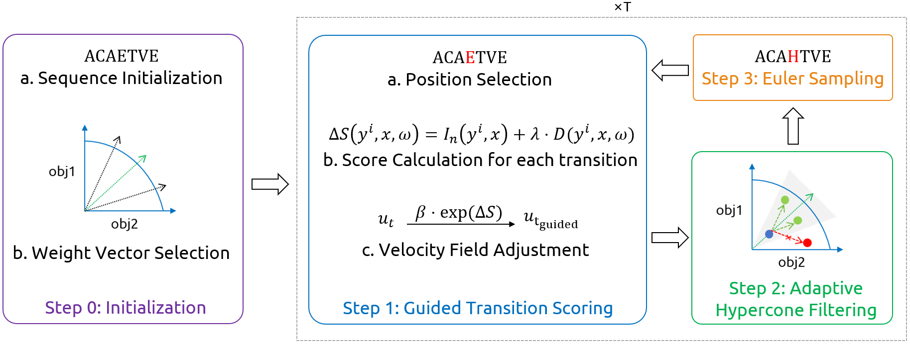
To achieve this, we will guide the CTMC sampling dynamics of the discrete flow matching model using multi-objective transition scores, steering the generative process toward Pareto-efficient regions of the state space (Figure 1, Pseudocode 1, Proof in Section D).
3.1 Step 0: Initialization and Weight Vector Generation
MOG-DFM begins by initializing the generative process at time by sampling an initial sequence uniformly from the discrete state space . To steer the generation towards diverse Pareto-efficient solutions, we introduce a set of weight vectors , where , that uniformly cover the -dimensional Pareto front. Intuitively, each encodes a particular trade-off among the objectives, so sampling different promotes exploration of distinct regions of the Pareto front. We construct these vectors via the Das–Dennis simplex lattice with subdivisions, yielding components
| (11) |
and then draw one randomly before the following steps. This defines one direction we want to optimize toward the Pareto front in the current run. The following three steps will then be performed in each iteration. We set the number of total iterations to .
3.2 Step 1: Guided Transition Scoring
We first randomly select one position in the sequence that will be updated during the current iteration. At each intermediate state and selected position , each possible candidate transition is scored by combining local improvement measures with global directional alignment. The normalized rank score captures how much each individual objective improves relative to other possible token replacements, thereby encouraging exploration of promising local moves. Formally, for each objective we compute
| (12) |
where denotes the sequence obtained by replacing the th token of with . The function maps the raw score change into a uniform scale in . In contrast, the directional term
| (13) |
measures the alignment of the multi-objective improvement vector with the chosen weight vector , ensuring that transitions not only improve individual objectives but collectively move toward the desired trade-off direction. To balance rank-based exploration against direction-guided exploitation, we z-score normalize both components and combine them as follows
| (14) |
where is a tunable hyperparameter. An importance vector is used to normalize the improvement values for each objective. Finally, we re-weight the original factorized velocity field from the pre-trained discrete flow matching model:
| (15) |
where is the strength hyperparameter. Therefore, the guided velocities satisfy the non-negativity and zero-sum rate conditions by construction, preserving valid CTMC dynamics while favoring high-utility transitions.
3.3 Step 2: Adaptive Hypercone Filtering
To ensure each candidate token replacement drives the sequence towards the chosen trade-off direction, we restrict candidate transitions to lie within a cone around the weight vector . This “hypercone” mechanism allows the sampler to navigate non-convex or discontinuous regions of the Pareto front by enforcing local directional consistency. Specifically, for a given position and candidate token , we compute the angle
| (16) |
where is the multi-objective improvement vector from replacing with . We accept only those for which , where denotes the current hypercone angle. Denoting as the set of accepted tokens, we select the best transition as
| (17) |
There are two degenerate cases that can lead to empty : (1) if every , indicating that all possible transitions decrease performance, we will perform a self-transition and retain the current state; (2) if there exist some but none lie within the cone (i.e., is temporarily too small), we still advance by choosing the best-aligned candidate
| (18) |
allowing progress while the hypercone angle self-adjusts.
As a pre-defined hypercone angle may be too big or too small during the dynamic optimization process, we need to adaptively tune the angle that best balances exploration and exploitation. Specifically, we compute the rejection rate
| (19) |
and its exponential moving average (EMA)
| (20) |
where is a smoothing coefficient and is the target rejection rate. We then update the hypercone angle via
| (21) |
with learning rate and bounds to prevent the hypercone from collapsing or over-expanding. Intuitively, if too many candidates are being rejected (), the hypercone widens to admit more directions; if too few are rejected (), it narrows to focus on the most aligned transitions.
3.4 Step 3: Euler Sampling
Once the guided transition rates have been computed and the best candidate transition has been selected after hypercone filtering (if not self-transitioning), we evolve the CTMC via Euler sampling. Specifically, we denote the total outgoing rate from at time on coordinate by
| (22) |
The one-step transition kernel for coordinate is given by the exact Euler–Maruyama analogue for CTMCs:
| (23) |
Here, is the step size in the time interval, and denotes the current state and the next state respectively. In practice, one draws a uniform random number : if , will transition to the best selected candidate; otherwise, we retain .
After performing step 1 to step 3 for iterations, we end with the final sample whose score vectors have been steered close to the Pareto front, with all objectives optimized.
4 Experiments
To the best of our knowledge, there are no public datasets that serve to benchmark multi-objective optimization algorithms for biological sequences. Therefore, we develop two benchmarks to evaluate MOG-DFM: multi-objective guided peptide binder sequence generation and multi-objective guided enhancer DNA sequence generation. We first show two discrete flow matching models developed for peptide generation and enhancer DNA generation, and we then demonstrate MOG-DFM’s efficacy on a wide variety of tasks and examples.
4.1 PepDFM and EnhancerDFM Generate Diverse and Biologically Plausible Sequences
To enable the efficient generation of peptide binders, we developed an unconditional peptide generator, PepDFM, based on the Discrete Flow Matching (DFM) framework. The model backbone of PepDFM is a U-Net-style convolutional architecture. We trained PepDFM on a custom dataset that includes all peptides from the PepNN and BioLip2 datasets, as well as sequences from the PPIRef dataset with lengths ranging from 6 to 49 amino acids, finally converging to a training loss of 3.3134 and a validation loss of 3.1051 [31, 32, 33]. As described in Section 2, the low generalized KL loss during evaluation demonstrates the strong performance of PepDFM. We further investigate the diversity and biological plausibility of peptides generated by PepDFM. Specifically, PepDFM generates peptides with substantially high Hamming distances from the test set, indicating a great degree of diversity and novelty in the generated sequences (Figure 3). Additionally, the Shannon entropy of the generated peptides closely matches that of the test set, highlighting the model’s capability to produce biologically plausible peptides with diverse sequence lengths (Figure 3).
| FBD | NFE | # Training Epochs | |
| Random Sequence | 622.8 | - | - |
| Dirichlet FM | 5.3 | 100 | 1400 |
| EnhancerDFM | 5.9 | 100 | 20 |
EnhancerDFM adopts the same model backbone and melanoma enhancer dataset used in the enhancer DNA design task from Stark, et al. [27]. We employed the Fréchet Biological distance (FBD) metric from [27] to evaluate the performance of EnhancerDFM (Table 1). Specifically, using the same number of function evaluations (NFE), EnhancerDFM achieved a comparable FBD of 5.9 compared with Dirichlet FM of 5.3, significantly lower than the FBD of random sequences, demonstrating EnhancerDFM’s ability to design biologically plausible enhancer DNA sequences. Significantly, the best EnhancerDFM model is achieved within 20 training epochs, while the best EnhancerDFM is obtained only in around 1400 training epochs, highlighting discrete flow matching models’ superior capability of capturing the underlying data distribution.
4.2 MOG-DFM effectively balances each objective trade-off
To validate that the MOG-DFM framework can balance the trade-offs between each objective, we performed two sets of experiments for peptide binder generation with three property guidance, and in ablation experiment settings, we removed one or more objectives. In the binder design task for target 7LUL (affinity, solubility, hemolysis guidance; Table 8), omitting any single guidance causes a collapse in that property, while the remaining guided metrics may modestly improve. Likewise, in the binder design task for target CLK1 (affinity, non-fouling, half-life guidance; Table 9), disabling non-fouling guidance allows half-life to exceed 80 hours but drives non-fouling near zero, and disabling half-life guidance preserves non-fouling yet reduces half-life below 2 hours. In contrast, enabling all guidance signals produces the most balanced profiles across all objectives. These results confirm that MOG-DFM precisely targets chosen objectives while preserving the flexibility to navigate conflicting requirements and push samples toward the Pareto front, thereby demonstrating the correctness and precision of our multi-objective sampling framework.
| Target | Binder Length | Hemolysis () | Non-Fouling () | Solubility () | Half-Life () | Affinity () |
| AMHR2 | 8 | 0.0755 | 0.8352 | 0.8219 | 31.624 | 7.3789 |
| AMHR2 | 12 | 0.0570 | 0.8419 | 0.8279 | 28.761 | 7.4274 |
| AMHR2 | 16 | 0.0618 | 0.7782 | 0.7428 | 31.227 | 7.6099 |
| EWS::FLI1 | 8 | 0.0809 | 0.8508 | 0.8296 | 47.169 | 6.2251 |
| EWS::FLI1 | 12 | 0.0616 | 0.8302 | 0.8130 | 34.225 | 6.3631 |
| EWS::FLI1 | 16 | 0.0709 | 0.7787 | 0.7400 | 34.192 | 6.5912 |
| MYC | 8 | 0.0809 | 0.8135 | 0.8005 | 39.836 | 6.8488 |
| OX1R | 10 | 0.0741 | 0.8115 | 0.7969 | 33.533 | 7.4162 |
| DUSP12 | 9 | 0.0735 | 0.8360 | 0.8216 | 33.754 | 6.4946 |
| 1B8Q | 8 | 0.0744 | 0.8334 | 0.827 | 33.243 | 5.932 |
| 1E6I | 6 | 0.0887 | 0.7884 | 0.7793 | 41.164 | 4.9621 |
| 3IDJ | 7 | 0.0924 | 0.8246 | 0.7992 | 30.388 | 7.6304 |
| 5AZ8 | 11 | 0.0698 | 0.8462 | 0.8420 | 28.726 | 6.6051 |
| 7JVS | 11 | 0.0628 | 0.8390 | 0.8206 | 32.834 | 6.9569 |
4.3 MOG-DFM generates peptide binders under five property guidance
We next benchmark MOG-DFM on a peptide binder generation task guided by five different properties that are critical for therapeutic discovery: hemolysis, non-fouling, solubility, half-life, and binding affinity. To evaluate MOG-DFM in a controlled setting, we designed 100 peptide binders per target for ten diverse proteins—structured targets with known binders (1B8Q, 1E6I, 3IDJ, 5AZ8, 7JVS), structured targets without known binders (AMHR2, OX1R, DUSP12), and intrinsically disordered targets (EWS::FLI1, MYC) (Table 2). Across all targets and across multiple binder lengths, the generated peptides achieve low hemolysis rates (0.06–0.09), high non-fouling (0.78) and solubility (0.74), extended half-life (28–47 h), and strong affinity scores (6.4–7.6), demonstrating both balanced optimization and robustness to sequence length.
For the target proteins with pre-existing binders, we compared the property values between their known binders with MOG-DFM-designed ones (Figure 2A,B, 4). The designed binders significantly outperform the pre-existing binders across all properties without compromising the binding potential, which is further confirmed by the ipTM scores computed by AlphaFold3 [34] and docking scores calculated by AutoDock VINA [35]. Although the MOG-DFM-designed binders bind to similar target positions as the pre-existing ones, they differ significantly in sequence and structure, demonstrating MOG-DFM’s capacity to explore the vast sequence space for optimal designs. For target proteins without known binders, complex structures were visualized using one of the MOG-DFM-designed binders (Figure 2C,D, 5). The corresponding property scores, as well as ipTM and docking scores, are also displayed. Some of the designed binders demonstrated extended half-life, while others excelled in non-fouling and solubility, underscoring the comprehensive exploration of the sequence space by MOG-DFM.


At each iteration, we recorded the mean and standard deviation of the five property scores across all the 100 binders to evaluate the effectiveness of the guided generation strategy (Figure 2E). All five properties exhibited an improving trend over iterations, with the average score of the solubility and non-fouling properties showing a significant increase from score around 0.3 to 0.8. A large deviation of the final half-life values is caused by the susceptibility of the half-life value to guidance, with MOG-DFM balancing the trade-offs between half-life and other values. The improvements of hemolysis, non-fouling, and solubility gradually converge, demonstrating MOG-DFM’s efficiency in steering the generation process to the Pareto Front within only 100 iterations.
We visualized the distribution change steered by MOG-DFM by plotting the property score distribution of 100 peptides of length 12 designed for EWS::FLI1 and 100 peptides of the same length sampled unconditionally from PepDFM (Figure 2F). MOG-DFM effectively shifted and concentrated the peptide distribution so that the peptides possess improved properties for all the objectives, demonstrating MOG-DFM’s ability to steer the generation so that all properties are optimized simultaneously.
In Section B, we demonstrate the reliability of our score models. We now use external evaluation tools to further confirm that MOG-DFM-designed binders possess desired properties. The average solubility and half-life for each target across all 100 designed peptides were predicted using ADMET-AI (Table 6) [36]. ADMET-AI, trained on a different dataset from our solubility and half-life prediction models, predicts average LogS values around –2.5 , which is well above the conventional –4 threshold for good solubility, and confirms long half-life estimates (>15 h). These results from an orthogonal predictive model demonstrate MOG-DFM’s capability to generate candidates with multiple desirable drug properties.
| Target | Method | Time (s) | Hemolysis () | Non-Fouling | Solubility | Half-Life | Affinity |
| 1B8Q | MOPSO | 8.54 | 0.1066 | 0.4763 | 0.4684 | 4.449 | 6.0594 |
| NSGA-III | 33.13 | 0.0862 | 0.5715 | 0.5825 | 7.324 | 7.2178 | |
| SMS-EMOA | 8.21 | 0.1196 | 0.3450 | 0.3511 | 3.023 | 5.955 | |
| SPEA2 | 17.48 | 0.0819 | 0.4973 | 0.5057 | 4.126 | 7.324 | |
| MOG-DFM | 43.00 | 0.0785 | 0.8445 | 0.8455 | 27.227 | 5.9094 | |
| PPP5 | MOPSO | 11.34 | 0.0883 | 0.4711 | 0.4255 | 1.769 | 6.6958 |
| NSGA-III | 37.30 | 0.0479 | 0.7138 | 0.7066 | 2.901 | 7.3789 | |
| SMS-EMOA | 8.43 | 0.1242 | 0.4269 | 0.4334 | 1.031 | 6.2854 | |
| SPEA2 | 19.02 | 0.0555 | 0.6221 | 0.6098 | 2.613 | 7.6253 | |
| MOG-DFM | 90.00 | 0.0617 | 0.7738 | 0.751 | 27.775 | 6.8197 |
We benchmarked MOG-DFM against four multi-objective optimizers—NSGA-III [37], SMS-EMOA [38], SPEA2 [39], and MOPSO [40]—on two protein targets: 1B8Q (a small protein with known peptide binders) and PPP5 (a larger protein lacking characterized binders) (Table 3). For each method, we generated 100 peptide binders per target of a specified length, guided by five property objectives (hemolysis, non-fouling, solubility, half-life, and binding affinity), and recorded both the average generation time for one sequence and the mean property scores. Although MOG-DFM requires longer runtimes, it consistently produces the most favorable trade-offs: reducing predicted hemolysis by more than 10%, boosting non-fouling and solubility by approximately 30-50%, and extending half-life by a factor of 3 to 4 compared to the next-best method, while maintaining competitive affinity values. These results demonstrate MOG-DFM’s effectiveness in navigating high-dimensional property landscapes to generate peptide binders with well-balanced, optimized profiles. We did not benchmark against ParetoFlow, another multi-objective optimization algorithm that uses flow matching, because it requires score models to take continuous inputs, which is not suitable for our task [20].
4.4 Hyperparameter Sensitivity Benchmark
There are several hyperparameters in MOG-DFM whose settings may affect generative performance. To assess this sensitivity, we evaluated peptide binder design across a broad range of values for each parameter (Table 10). We find that increasing the number of sampling steps consistently improves all performance metrics, as finer discretization more closely approximates the continuous-time dynamics. In contrast, setting the initial hypercone angle too small or too large both degrade results: an overly narrow cone restricts exploration, while an overly wide cone dilutes directional guidance. The importance weights also play a critical role in balancing multiple objectives. Because each property can vary over a different numerical range, we initialize each weight inversely proportional to the maximum observed improvement of that property, thereby normalizing all guidance signals to roughly unit scale. This allows for similar improvements for each objective, otherwise the improvements for some objectives may stagnate. By comparison, the remaining hyperparameters (i.e., , , , , , and the bounds ) exhibit only modest impact on outcomes, indicating that MOG-DFM is robust to moderate variations in these settings.
4.5 Adaptive Hypercone Filtering Enhances Multi-Objective Optimization
To quantify the contribution of our adaptive hypercone mechanism, we performed an ablation study on three increasingly disordered, and thus undruggable, protein targets (3IDJ, 4E-BP2, and EWS::FLI1), generating 100 peptide binders for each target (Table 7). Removing hypercone filtering entirely (“w/o filtering”) causes a dramatic collapse in half-life—from roughly 30–35 hours down to 4–13 hours—while leaving non-fouling and solubility largely unchanged, indicating that filtering out poorly aligned moves is essential for optimizing objectives that require gradual, coordinated changes. Introducing static hypercone gating without angle adaptation (“w/o adaptation”) recovers much of the half-life gains (to 23–37 h), but at the expense of reduced non-fouling and solubility scores and only marginal improvements in affinity. In contrast, the full MOG-DFM—with both directional hypercone filtering and adaptive angle updates—simultaneously elevates half-life and maintains strong performance across all five objectives. This effect is especially pronounced on disordered targets (4E-BP2 and EWS::FLI1), where dynamic cone adjustment is essential for navigating the irregular, non-convex Pareto landscapes.
| Guidance Settings | Task 1 | Task 2 | |||
| Shape | Class | Class Prob | Shape | Class Prob | Shape |
| ✓ | ✓ | 0.7504 | 36.0100 | 0.9960 | 3.3640 |
| 0.6507 | 36.0100 | 0.9922 | 3.3680 | ||
| 0.6821 | 36.0000 | 0.9864 | 3.3669 | ||
| 0.7097 | 36.0000 | 0.9976 | 3.3680 | ||
| 0.6425 | 36.0000 | 0.9961 | 3.3623 | ||
| 0.9999 | 34.3274 | 1.0000 | 3.3368 | ||
| 0.9999 | 34.4715 | 1.0000 | 3.3345 | ||
| 0.9989 | 34.4257 | 0.9999 | 3.3348 | ||
| 0.9997 | 34.5226 | 0.9994 | 3.3357 | ||
| 0.9998 | 34.4210 | 1.0000 | 3.3340 | ||
| 0.0026 | 36.0017 | 2.36E-05 | 3.3690 | ||
| 0.0055 | 36.0238 | 0.0005 | 3.3647 | ||
| 0.0062 | 36.0214 | 0.0114 | 3.3705 | ||
| 0.0186 | 36.0396 | 0.0001 | 3.3717 | ||
| 0.0051 | 36.0304 | 0.0054 | 3.3669 | ||
| 0.0362 | 34.7379 | 0.0008 | 3.3283 | ||
| 0.0364 | 34.5350 | 0.0057 | 3.3258 | ||
| 0.0309 | 34.5720 | 0.0476 | 3.3268 | ||
| 0.0138 | 34.3060 | 0.0632 | 3.3378 | ||
| 0.0213 | 34.5500 | 0.0003 | 3.3320 | ||
4.6 MOG-DFM generates enhancer DNA of specific class with specified DNA shapes
To demonstrate the universal capability of MOG-DFM in performing multi-objective guided generation for biological sequences, we applied MOG-DFM to design enhancer DNA sequences guided by enhancer class and DNA shape. EnhancerDFM was used as the unconditional enhancer DNA sequence generator, while Deep DNAshape was employed to predict DNA shape [41], and the enhancer class predictor from which it was sourced [27]. Two distinct tasks with different enhancer class and DNA shape guidance were carried out, and ablation results are presented in Table 4. Given the time constraints, we designed five enhancer sequences of length 100 for each setting.
In the first task, we conditioned the generation to target enhancer class 1 (associated with the transcription factor binding motif ATF) and a high HelT (helix twist) value, with the maximum HelT value set to 36. With both guidance criteria in place, MOG-DFM effectively steered the sequence generation towards enhancer class 1 while simultaneously ensuring that the HelT value approached its maximum (Table 4). When one or both guidance criteria were removed, the corresponding properties showed significant degradation, with the probability of achieving the desired enhancer class dropping near zero (Table 4). A similar outcome was observed in the second task, which targeted enhancer class 16 and a higher Rise shape value, with the maximum Rise value set to 3.7. Since the canonical range for the Rise shape value spans from 3.3 to 3.4, MOG-DFM ensured both a high probability for the target enhancer class and an optimal DNA shape value, outperforming other ablation settings (Table 4).
5 Conclusion
In this work, we have presented Multi-Objective-Guided Discrete Flow Matching (MOG-DFM), a scalable framework for generating biomolecular sequences that simultaneously optimize multiple, often conflicting properties. By guiding discrete flow matching models with multi-objective optimization, MOG-DFM enables the design of peptide and DNA sequences with improved therapeutic and structural characteristics.
While MOG-DFM performs well in biological domains, future work will extend the framework to longer sequences and higher-dimensional outputs, including applications in text and image generation. From a theoretical perspective, improving Pareto convergence guarantees and incorporating uncertainty-aware or feedback-driven guidance remain key directions to explore. Ultimately, MOG-DFM offers a foundation for generating the next generation of therapeutics—molecules that are not only effective but explicitly optimized for the multifaceted properties critical to clinical success.
6 Declarations
Acknowledgments. We thank the Duke Compute Cluster, Pratt School of Engineering IT department, and Mark III Systems, for providing database and hardware support that has contributed to the research reported within this manuscript.
Author Contributions. T.C. devised model architectures and theoretical formulations, and trained and benchmarked models. Y.Z. trained and benchmarked supervised models, and performed molecular docking. Y.Z. and S.T. advised on model design and theoretical framework. T.C. drafted the manuscript, and Y.Z. and S.T. assisted in figure design and data presentation. P.C. designed, supervised, and directed the study, formulated algorithm proofs, and finalized the manuscript.
Data and Materials Availability. The codebase will be freely accessible to the academic community at https://huggingface.co/ChatterjeeLab/MOG-DFM.
Funding Statement. This research was supported by grants from the Hartwell Foundation, CHDI Foundation, and EndAxD Foundation to the lab of P.C.
Competing Interests. P.C. is a co-founder of Gameto, Inc. and UbiquiTx, Inc. and advises companies involved in biologics development. P.C.’s interests are reviewed and managed by Duke University in accordance with their conflict-of-interest policies. T.C., S.T., and Y.Z., have no conflicts of interest to declare.
References
- [1] Gita Naseri and Mattheos AG Koffas. Application of combinatorial optimization strategies in synthetic biology. Nature communications, 11(1):2446, 2020.
- [2] Masahiro Tominaga, Yoko Shima, Kenta Nozaki, Yoichiro Ito, Masataka Someda, Yuji Shoya, Noritaka Hashii, Chihiro Obata, Miho Matsumoto-Kitano, Kohei Suematsu, et al. Designing strong inducible synthetic promoters in yeasts. Nature Communications, 15(1):10653, 2024.
- [3] Stephanie E Mohr, Yanhui Hu, Benjamin Ewen-Campen, Benjamin E Housden, Raghuvir Viswanatha, and Norbert Perrimon. Crispr guide rna design for research applications. The FEBS journal, 283(17):3232–3238, 2016.
- [4] Henri Schmidt, Minsi Zhang, Dimitar Chakarov, Vineet Bansal, Haralambos Mourelatos, Francisco J Sánchez-Rivera, Scott W Lowe, Andrea Ventura, Christina S Leslie, and Yuri Pritykin. Genome-wide crispr guide rna design and specificity analysis with guidescan2. Genome biology, 26(1):1–25, 2025.
- [5] Valentin Artemyev, Anna Gubaeva, Anastasiia Iu Paremskaia, Amina A Dzhioeva, Andrei Deviatkin, Sofya G Feoktistova, Olga Mityaeva, and Pavel Yu Volchkov. Synthetic promoters in gene therapy: Design approaches, features and applications. Cells, 13(23):1963, 2024.
- [6] Ruimin Zhou, Zhaoyan Jiang, Chen Yang, Jianwei Yu, Jirui Feng, Muhammad Abdullah Adil, Dan Deng, Wenjun Zou, Jianqi Zhang, Kun Lu, et al. All-small-molecule organic solar cells with over 14% efficiency by optimizing hierarchical morphologies. Nature communications, 10(1):5393, 2019.
- [7] Atef Nehdi, Nosaibah Samman, Vanessa Aguilar-Sánchez, Azer Farah, Emre Yurdusev, Mohamed Boudjelal, and Jonathan Perreault. Novel strategies to optimize the amplification of single-stranded dna. Frontiers in Bioengineering and Biotechnology, 8:401, 2020.
- [8] Ryan P Kreiser, Aidan K Wright, Natalie R Block, Jared E Hollows, Lam T Nguyen, Kathleen LeForte, Benedetta Mannini, Michele Vendruscolo, and Ryan Limbocker. Therapeutic strategies to reduce the toxicity of misfolded protein oligomers. International journal of molecular sciences, 21(22):8651, 2020.
- [9] Neelam Sharma, Leimarembi Devi Naorem, Shipra Jain, and Gajendra PS Raghava. Toxinpred2: an improved method for predicting toxicity of proteins. Briefings in bioinformatics, 23(5):bbac174, 2022.
- [10] Evan Komp, Christian Phillips, Lauren M Lee, Shayna M Fallin, Humood N Alanzi, Marlo Zorman, Michelle E McCully, and David AC Beck. Neural network conditioned to produce thermophilic protein sequences can increase thermal stability. Scientific Reports, 15(1):14124, 2025.
- [11] Alessandra Bigi, Eva Lombardo, Roberta Cascella, and Cristina Cecchi. The toxicity of protein aggregates: new insights into the mechanisms, 2023.
- [12] Dillon J Rinauro, Fabrizio Chiti, Michele Vendruscolo, and Ryan Limbocker. Misfolded protein oligomers: Mechanisms of formation, cytotoxic effects, and pharmacological approaches against protein misfolding diseases. Molecular Neurodegeneration, 19(1):20, 2024.
- [13] Eckart Zitzler and Lothar Thiele. Multiobjective optimization using evolutionary algorithms—a comparative case study. In International conference on parallel problem solving from nature, pages 292–301. Springer, 1998.
- [14] Kalyanmoy Deb. Multi-objective optimisation using evolutionary algorithms: an introduction. In Multi-objective evolutionary optimisation for product design and manufacturing, pages 3–34. Springer, 2011.
- [15] Tsuyoshi Ueno, Trevor David Rhone, Zhufeng Hou, Teruyasu Mizoguchi, and Koji Tsuda. Combo: An efficient bayesian optimization library for materials science. Materials discovery, 4:18–21, 2016.
- [16] Trevor S Frisby and Christopher James Langmead. Bayesian optimization with evolutionary and structure-based regularization for directed protein evolution. Algorithms for Molecular Biology, 16(1):13, 2021.
- [17] Yibo Li, Liangren Zhang, and Zhenming Liu. Multi-objective de novo drug design with conditional graph generative model. Journal of cheminformatics, 10:1–24, 2018.
- [18] Tiago Sousa, João Correia, Vitor Pereira, and Miguel Rocha. Combining multi-objective evolutionary algorithms with deep generative models towards focused molecular design. In Applications of Evolutionary Computation: 24th International Conference, EvoApplications 2021, Held as Part of EvoStar 2021, Virtual Event, April 7–9, 2021, Proceedings 24, pages 81–96. Springer, 2021.
- [19] Yinghua Yao, Yuangang Pan, Jing Li, Ivor Tsang, and Xin Yao. Proud: Pareto-guided diffusion model for multi-objective generation. Machine Learning, 113(9):6511–6538, 2024.
- [20] Ye Yuan, Can Chen, Christopher Pal, and Xue Liu. Paretoflow: Guided flows in multi-objective optimization. arXiv preprint arXiv:2412.03718, 2024.
- [21] Gleb Beliakov and Kieran F Lim. Challenges of continuous global optimization in molecular structure prediction. European journal of operational research, 181(3):1198–1213, 2007.
- [22] Richard Michael, Simon Bartels, Miguel González-Duque, Yevgen Zainchkovskyy, Jes Frellsen, Søren Hauberg, and Wouter Boomsma. A continuous relaxation for discrete bayesian optimization. arXiv preprint arXiv:2404.17452, 2024.
- [23] Sophia Tang, Yinuo Zhang, and Pranam Chatterjee. Peptune: De novo generation of therapeutic peptides with multi-objective-guided discrete diffusion. Proceedings of the 42nd International Conference on Machine Learning (ICML), 2025a.
- [24] Subham Sekhar Sahoo, Marianne Arriola, Yair Schiff, Aaron Gokaslan, Edgar Marroquin, Justin T Chiu, Alexander Rush, and Volodymyr Kuleshov. Simple and effective masked diffusion language models. Advances in Neural Information Processing Systems, 2024.
- [25] Itai Gat, Tal Remez, Neta Shaul, Felix Kreuk, Ricky TQ Chen, Gabriel Synnaeve, Yossi Adi, and Yaron Lipman. Discrete flow matching. Advances in Neural Information Processing Systems, 37:133345–133385, 2024.
- [26] Ian Dunn and David Ryan Koes. Exploring discrete flow matching for 3d de novo molecule generation. ArXiv, pages arXiv–2411, 2024.
- [27] Hannes Stark, Bowen Jing, Chenyu Wang, Gabriele Corso, Bonnie Berger, Regina Barzilay, and Tommi Jaakkola. Dirichlet flow matching with applications to dna sequence design. Proceedings of the 41st International Conference on Machine Learning (ICML), 2024.
- [28] Oscar Davis, Samuel Kessler, Mircea Petrache, Ismail Ceylan, Michael Bronstein, and Joey Bose. Fisher flow matching for generative modeling over discrete data. Advances in Neural Information Processing Systems, 37:139054–139084, 2024.
- [29] Sophia Tang, Yinuo Zhang, Alexander Tong, and Pranam Chatterjee. Gumbel-softmax flow matching with straight-through guidance for controllable biological sequence generation. arXiv preprint arXiv:2503.17361, 2025b.
- [30] Hunter Nisonoff, Junhao Xiong, Stephan Allenspach, and Jennifer Listgarten. Unlocking guidance for discrete state-space diffusion and flow models. Proceedings of the 13th International Conference on Learning Representations (ICLR), 2025.
- [31] Osama Abdin, Satra Nim, Han Wen, and Philip M Kim. Pepnn: a deep attention model for the identification of peptide binding sites. Communications biology, 5(1):503, 2022.
- [32] Chengxin Zhang, Xi Zhang, Peter L Freddolino, and Yang Zhang. Biolip2: an updated structure database for biologically relevant ligand–protein interactions. Nucleic Acids Research, 52(D1):D404–D412, 2024.
- [33] Anton Bushuiev, Roman Bushuiev, Petr Kouba, Anatolii Filkin, Marketa Gabrielova, Michal Gabriel, Jiri Sedlar, Tomas Pluskal, Jiri Damborsky, Stanislav Mazurenko, et al. Learning to design protein-protein interactions with enhanced generalization. arXiv preprint arXiv:2310.18515, 2023.
- [34] Josh Abramson, Jonas Adler, Jack Dunger, Richard Evans, Tim Green, Alexander Pritzel, Olaf Ronneberger, Lindsay Willmore, Andrew J Ballard, Joshua Bambrick, et al. Accurate structure prediction of biomolecular interactions with alphafold 3. Nature, 630(8016):493–500, 2024.
- [35] Oleg Trott and Arthur J Olson. Autodock vina: improving the speed and accuracy of docking with a new scoring function, efficient optimization, and multithreading. Journal of computational chemistry, 31(2):455–461, 2010.
- [36] Kyle Swanson, Parker Walther, Jeremy Leitz, Souhrid Mukherjee, Joseph C Wu, Rabindra V Shivnaraine, and James Zou. Admet-ai: a machine learning admet platform for evaluation of large-scale chemical libraries. Bioinformatics, 40(7):btae416, 2024.
- [37] Kalyanmoy Deb and Himanshu Jain. An evolutionary many-objective optimization algorithm using reference-point-based nondominated sorting approach, part i: solving problems with box constraints. IEEE transactions on evolutionary computation, 18(4):577–601, 2013.
- [38] Nicola Beume, Boris Naujoks, and Michael Emmerich. Sms-emoa: Multiobjective selection based on dominated hypervolume. European journal of operational research, 181(3):1653–1669, 2007.
- [39] Eckart Zitzler, Marco Laumanns, and Lothar Thiele. Spea2: Improving the strength pareto evolutionary algorithm. TIK report, 103, 2001.
- [40] CA Coello Coello and Maximino Salazar Lechuga. Mopso: A proposal for multiple objective particle swarm optimization. In Proceedings of the 2002 Congress on Evolutionary Computation. CEC’02 (Cat. No. 02TH8600), volume 2, pages 1051–1056. IEEE, 2002.
- [41] Jinsen Li, Tsu-Pei Chiu, and Remo Rohs. Predicting dna structure using a deep learning method. Nature communications, 15(1):1243, 2024.
- [42] Olaf Ronneberger, Philipp Fischer, and Thomas Brox. U-net: Convolutional networks for biomedical image segmentation. In Medical image computing and computer-assisted intervention–MICCAI 2015: 18th international conference, Munich, Germany, October 5-9, 2015, proceedings, part III 18, pages 234–241. Springer, 2015.
- [43] Zeming Lin, Halil Akin, Roshan Rao, Brian Hie, Zhongkai Zhu, Wenting Lu, Nikita Smetanin, Robert Verkuil, Ori Kabeli, Yaniv Shmueli, et al. Evolutionary-scale prediction of atomic-level protein structure with a language model. Science, 379(6637):1123–1130, 2023.
- [44] Zeynep Kalender Atak, Ibrahim Ihsan Taskiran, Jonas Demeulemeester, Christopher Flerin, David Mauduit, Liesbeth Minnoye, Gert Hulselmans, Valerie Christiaens, Ghanem-Elias Ghanem, Jasper Wouters, et al. Interpretation of allele-specific chromatin accessibility using cell state–aware deep learning. Genome research, 31(6):1082–1096, 2021.
- [45] Jason D Buenrostro, Paul G Giresi, Lisa C Zaba, Howard Y Chang, and William J Greenleaf. Transposition of native chromatin for fast and sensitive epigenomic profiling of open chromatin, dna-binding proteins and nucleosome position. Nature methods, 10(12):1213–1218, 2013.
- [46] Ruochi Zhang, Haoran Wu, Yuting Xiu, Kewei Li, Ningning Chen, Yu Wang, Yan Wang, Xin Gao, and Fengfeng Zhou. Pepland: a large-scale pre-trained peptide representation model for a comprehensive landscape of both canonical and non-canonical amino acids. arXiv preprint arXiv:2311.04419, 2023.
- [47] Chakradhar Guntuboina, Adrita Das, Parisa Mollaei, Seongwon Kim, and Amir Barati Farimani. Peptidebert: A language model based on transformers for peptide property prediction. The Journal of Physical Chemistry Letters, 14(46):10427–10434, 2023.
- [48] F. Pedregosa, G. Varoquaux, A. Gramfort, V. Michel, B. Thirion, O. Grisel, M. Blondel, P. Prettenhofer, R. Weiss, V. Dubourg, J. Vanderplas, A. Passos, D. Cournapeau, M. Brucher, M. Perrot, and E. Duchesnay. Scikit-learn: Machine learning in Python. Journal of Machine Learning Research, 12:2825–2830, 2011.
- [49] Takuya Akiba, Shotaro Sano, Toshihiko Yanase, Takeru Ohta, and Masanori Koyama. Optuna: A next-generation hyperparameter optimization framework. In International Conference on Knowledge Discovery and Data Mining, pages 2623–2631, 2019.
- [50] Deepika Mathur, Satya Prakash, Priya Anand, Harpreet Kaur, Piyush Agrawal, Ayesha Mehta, Rajesh Kumar, Sandeep Singh, and Gajendra PS Raghava. Peplife: a repository of the half-life of peptides. Scientific reports, 6(1):36617, 2016.
- [51] Vera D’Aloisio, Paolo Dognini, Gillian A Hutcheon, and Christopher R Coxon. Peptherdia: database and structural composition analysis of approved peptide therapeutics and diagnostics. Drug Discovery Today, 26(6):1409–1419, 2021.
- [52] Shipra Jain, Srijanee Gupta, Sumeet Patiyal, and Gajendra PS Raghava. Thpdb2: compilation of fda approved therapeutic peptides and proteins. Drug Discovery Today, page 104047, 2024.
- [53] Kotaro Tsuboyama, Justas Dauparas, Jonathan Chen, Elodie Laine, Yasser Mohseni Behbahani, Jonathan J Weinstein, Niall M Mangan, Sergey Ovchinnikov, and Gabriel J Rocklin. Mega-scale experimental analysis of protein folding stability in biology and design. Nature, 620(7973):434–444, 2023.
Appendix A Base Model Details
A.1 PepDFM
Model Architecture. The base model is a time-dependent architecture based on U-Net [42]. It uses two separate embedding layers for sequence and time, followed by five convolutional blocks with varying dilation rates to capture temporal dependencies, while incorporating time-conditioning through dense layers. The final output layer generates logits for each token. We used a polynomial convex schedule with a polynomial exponent of 2.0 for the mixture discrete probability path in the discrete flow matching.
Dataset Curation. The dataset for PepDFM training was curated from the PepNN, BioLip2, and PPIRef dataset [31, 32, 33]. All peptides from PepNN and BioLip2 were included, along with sequences from PPIRef ranging from 6 to 49 amino acids in length. The dataset was divided into training, validation, and test sets at an 80/10/10 ratio.
Training Strategy. The training is conducted on a 2xH100 NVIDIA NVL GPU system with 94 GB of VRAM for 200 epochs with batch size 512. The model checkpoint with the lowest evaluation loss was saved. The Adam optimizer was employed with a learning rate 1e-4. A learning rate scheduler with 20 warm-up epochs and cosine decay was used, with initial and minimum learning rates both 1e-5. The embedding dimension and hidden dimension were set to be 512 and 256 respectively for the base model.
Dynamic Batching. To enhance computational efficiency and manage variable-length token sequences, we implemented dynamic batching. Drawing inspiration from ESM-2’s approach [43], input peptide sequences were sorted by length to optimize GPU memory utilization, with a maximum token size of 100 per GPU.
A.2 EnhancerDFM
Model Architecture. The base model for EnhancerDFM applies the same architecture as the PepDFM. We also used a polynomial convex schedule with a polynomial exponent of 2.0 for the mixture discrete probability path in the discrete flow matching.
Dataset Curation. The dataset for EnhancerDFM training is curated by [27]. The dataset contains 89k enhancer sequences from human melanoma cells [44]. Each sequence is of length 500 paired with cell class labels determined from ATAC-seq data [45]. There are 47 such classes of cells in total, with details displayed in Table 11 [44]. We applied the same dataset split strategy as [27].
Training Strategy. The training is conducted on a 2xH100 NVIDIA NVL GPU system with 94 GB of VRAM for 1500 epochs with batch size 256. The model checkpoint with the lowest evaluation loss was saved. The Adam optimizer was employed with a learning rate 1e-3. A learning rate scheduler with 150 warm-up epochs and cosine decay was used, with initial and minimum learning rates both 1e-4. Both the embedding dimension and hidden dimension were set to be 256 for the base model.
Appendix B Score Model Details
We collected hemolysis (9,316), non-fouling (17,185), solubility (18,453), and binding affinity (1,781) data for classifier training from the PepLand and PeptideBERT datasets [46, 47]. All sequences taken are wild-type L-amino acids and are tokenized and represented by ESM-2 protein language model [43].
B.1 Boosted Trees for Classification
For hemolysis, non-fouling, and solubility classification, we trained XGBoost boosted tree models for logistic regression. We split the data into 0.8/0.2 train/validation using traitified splits from scikit-learn [48] and generated mean pooled ESM-2-650M [43] embeddings as input features to the model. We ran 50 trials of OPTUNA [49] search to determine the optimal XGBoost hyperparameters (Table 5) tracking the best binary classification F1 scores. The best models for each property reached F1 scores of: 0.58, 0.71, and 0.68 on the validation sets accordingly.
| Hyperparameter | Value/Range |
| Objective | binary:logistic |
| Lambda | |
| Alpha | |
| Colsample by Tree | |
| Subsample | |
| Learning Rate | |
| Max Depth | |
| Min Child Weight | |
| Tree Method | hist |
B.2 Binding Affinity Score Model
We developed an unpooled reciprocal attention transformer model to predict protein-peptide binding affinity, leveraging latent representations from the ESM-2 650M protein language model [43]. Instead of relying on pooled representations, the model retains unpooled token-level embeddings from ESM-2, which are passed through convolutional layers followed by cross-attention layers. The binding affinity data was split into a 0.8/0.2 ratio, maintaining similar affinity score distributions across splits. We used OPTUNA [49] for hyperparameter optimization tracing validation correlation scores. The final model was trained for 50 epochs with a learning rate of 3.84e-5, a dropout rate of 0.15, 3 initial CNN kernel layers (dimension 384), 4 cross-attention layers (dimension 2048), and a shared prediction head (dimension 1024) in the end. The classifier reached 0.64 Spearman’s correlation score on validation data.
B.3 Half-Life Score Model
Dataset Curation. The half-life dataset is curated from three publicly available datasets: PEPLife, PepTherDia, and THPdb2 [50, 51, 52]. Data related to human subjects were selected, and entries with missing half-life values were excluded. After removing duplicates, the final dataset consists of 105 entries.
Pre-training on stability data. Given the small size of the half-life dataset, which is insufficient for training a model to capture the underlying data distribution, we first pre-trained a score model on a larger stability dataset to predict peptide stability [53]. The model consists of three linear layers with ReLU activation functions, and a dropout rate of 0.3 was applied. The model was trained on a 2xH100 NVIDIA NVL GPU system with 94 GB of VRAM for 50 epochs. The Adam optimizer was employed with a learning rate 1e-2. A learning rate scheduler with 5 warm-up epochs and cosine decay was used, with initial and minimum learning rates both 1e-3. After training, the model achieved a validation Spearman’s correlation of 0.7915 and an value of 0.6864, demonstrating the reliability of the stability score model.
Fine-tuning on half-life data. The pre-trained stability score model was subsequently fine-tuned on the half-life dataset. Since half-life values span a wide range, the model was adapted to predict the base-10 logarithm of the half-life (h) values to stabilize the learning process. After fine-tuning, the model achieved a validation Spearman’s correlation of 0.8581 and an value of 0.5977.
Appendix C Sampling Details
C.1 Peptide Binder Generation Tasks
Score Model Settings. To align all objectives as maximization, we convert the predicted hemolysis rate into a score , so that lower hemolysis yields a higher value. We also cap the predicted log-scale half-life at 2 (i.e., 100 hours) to prevent it from dominating the optimization and ensure balanced trade-offs across all properties. For the remaining objectives—non-fouling, solubility, and binding affinity—we directly employ their model outputs during sampling.
Hyperparameter Settings. The hyperparameters were set as follows: The number of divisions used in generating weight vectors, num_div, was set to 64, to 1.0, to 1.0, to 0.5, to 0.3, to 1.0, to , to , to . The total sampling step was 100.
Importance Vectors. In the task with five property guidance, the importance vector was set to , each corresponding to hemolysis, non-fouling, solubility, half-life, and binding affinity guidance, respectively. For the two tasks with only three property guidance, the importance vector was set to for solubility, hemolysis, and binding affinity guidance, respectively, and for non-fouling, half-life, and binding affinity guidance, respectively. The rationale for setting the importance values is based on the range lengths of the properties: hemolysis, non-fouling, and solubility each have a range length of 1.0, half-life has a range length of 2.0, and binding affinity has a range length of 10.0. The importance values were assigned inversely proportional to these range lengths.
C.2 Enhancer DNA Generation Tasks
Hyperparameter Settings. The hyperparameters were set the same as those in peptide binder generation tasks, except that the total sampling step was set to 800.
Importance Vectors. The importance vector was set to be [1, 10] for the first task and [1, 100] for the second task, with the first value corresponding to the enhancer class guidance and the second value corresponding to the DNA shape guidance. The rationale for assigning these importance values is based on the range lengths of the properties: enhancer class probability has a range length of 1.0, HelT shape values have a range length of 2.0, and Rise shape values have a range length of 0.1. The importance values were assigned inversely proportional to these range lengths.
Appendix D Additional Proof
Claim: MOG-DFM directs the discrete generation process toward the Pareto front by inducing a positive expected improvement in the direction of a specified weight vector .
Proof: Let be the discrete sequence space over vocabulary , and let denote the current sequence state at time . Assume the multi-objective score function is measurable, with scalar objectives. Define the improvement vector at a candidate transition at position as:
where denotes the sequence with token replaced by .
Let be a fixed unit-norm trade-off vector sampled uniformly from the Das–Dennis lattice covering the simplex . Define the directional improvement of a transition as:
Define the set of feasible transitions (those within the hypercone of angle ) at time as:
Let be the conditional probability measure over feasible transitions defined by:
where is the rank-directional guidance score and is the normalizing partition function. Assume that is non-empty, or else the algorithm falls back to selecting the best with by construction.
We now consider the expected improvement in the direction of over all guided transitions:
Since each satisfies , it follows that for all . Moreover, by construction.
Therefore, each term in the sum is strictly positive, and thus:
where is the updated sequence following a guided and filtered transition.
Hence, the MOG-DFM procedure ensures that in expectation, the sampling dynamics induce forward motion along the Pareto trade-off direction , thereby steering generation toward the Pareto frontier.
∎
| Target | LogS | Half-Life |
| AMHR2 | -2.3931 | 15.505 |
| AMHR2 | -2.5055 | 18.777 |
| AMHR2 | -2.5784 | 16.463 |
| EWS::FLI1 | -2.3869 | 18.945 |
| EWS::FLI1 | -2.3813 | 16.305 |
| EWS::FLI1 | -2.5457 | 15.984 |
| MYC | -2.4053 | 16.491 |
| OX1R | -2.4772 | 23.002 |
| DUSP12 | -2.4333 | 19.258 |
| 1B8Q | -2.3203 | 18.7862 |
| 1E6I | -2.0394 | 19.9358 |
| 3IDJ | -2.4193 | 20.3586 |
| 5AZ8 | -2.5964 | 16.3016 |
| 7JVS | -2.4824 | 20.2565 |
| Target | Method | Hemolysis () | Non-Fouling | Solubility | Half-Life | Affinity |
| 3IDJ | w/o filtering | 0.0660 | 0.8430 | 0.8482 | 12.50 | 7.3730 |
| w/o adaptation | 0.0856 | 0.8060 | 0.7970 | 37.17 | 7.3142 | |
| MOG-DFM | 0.0924 | 0.8246 | 0.7992 | 30.39 | 7.6304 | |
| 4E-BP2 | w/o filtering | 0.0504 | 0.8582 | 0.8600 | 12.62 | 6.5066 |
| w/o adaptation | 0.0638 | 0.8418 | 0.8234 | 23.44 | 6.4548 | |
| MOG-DFM | 0.0698 | 0.8210 | 0.8050 | 34.88 | 6.5824 | |
| EWS::FLI1 | w/o filtering | 0.0450 | 0.8596 | 0.8570 | 4.40 | 6.1392 |
| w/o adaptation | 0.0620 | 0.8444 | 0.8482 | 28.82 | 6.2118 | |
| MOG-DFM | 0.0616 | 0.8302 | 0.8130 | 34.225 | 6.3631 |
| Guidance Settings Affinity Solubility Hemolysis | Affinity | Solubility | Hemolysis () |
| 6.3489 | 0.8890 | 0.0620 | |
| 5.0514 | 0.9482 | 0.0406 | |
| 6.9060 | 0.4224 | 0.0488 | |
| 6.5304 | 0.8975 | 0.1019 | |
| 5.0761 | 0.7148 | 0.0163 | |
| 5.2434 | 0.9772 | 0.0955 | |
| 7.4834 | 0.1218 | 0.3281 | |
| 5.5631 | 0.3736 | 0.1567 |
| Guidance Settings Affinity Non-Fouling Half-Life | Affinity | Non-Fouling | Half-Life |
| 6.9194 | 0.7401 | 51.73 | |
| 6.4735 | 0.8107 | 60.75 | |
| 7.5360 | 0.3062 | 84.70 | |
| 7.4150 | 0.8560 | 1.24 | |
| 6.2363 | 0.2624 | 96.44 | |
| 6.1378 | 0.9503 | 0.94 | |
| 8.5943 | 0.2439 | 3.15 | |
| 5.8926 | 0.3999 | 1.94 |
| Hyper parameter | Target | Value | Hemolysis () | Non-Fouling | Solubility | Half-Life | Affinity |
| num_div | 6MLC | 32 | 0.0994 | 0.8088 | 0.7924 | 38.39 | 6.5436 |
| 64 | 0.0863 | 0.8280 | 0.8232 | 34.91 | 6.3260 | ||
| 128 | 0.0890 | 0.8438 | 0.8386 | 32.97 | 6.4197 | ||
| 4IU7 | 0.5 | 0.0829 | 0.7894 | 0.761 | 28.10 | 6.7884 | |
| 1 | 0.0684 | 0.8388 | 0.8321 | 41.78 | 7.0002 | ||
| 1.5 | 0.0585 | 0.8588 | 0.8582 | 47.65 | 7.0505 | ||
| 2 | 0.0615 | 0.8461 | 0.8416 | 53.45 | 7.0169 | ||
| 1AYC | 0.5 | 0.0703 | 0.8168 | 0.8152 | 30.89 | 6.4838 | |
| 1 | 0.0647 | 0.8362 | 0.8207 | 33.28 | 6.4549 | ||
| 2 | 0.0587 | 0.8690 | 0.8461 | 41.90 | 6.5317 | ||
| 2Q8Y | 0.1 | 0.0777 | 0.8361 | 0.8051 | 37.83 | 6.0569 | |
| 0.3 | 0.0718 | 0.8441 | 0.8280 | 38.83 | 6.0484 | ||
| 0.5 | 0.0718 | 0.8529 | 0.8421 | 31.45 | 6.0445 | ||
| 0.7 | 0.0688 | 0.8403 | 0.8377 | 35.50 | 6.0839 | ||
| 0.9 | 0.0813 | 0.8288 | 0.8091 | 45.25 | 6.1599 | ||
| 2LTV | 0.5 | 0.0633 | 0.8437 | 0.8368 | 29.48 | 7.3657 | |
| 1 | 0.0601 | 0.8256 | 0.8144 | 24.47 | 7.3111 | ||
| 2 | 0.0624 | 0.8125 | 0.7887 | 35.13 | 7.1974 | ||
| 5M02 | 15 | 0.0746 | 0.8285 | 0.8007 | 34.04 | 7.0335 | |
| 30 | 0.0792 | 0.8393 | 0.8187 | 35.60 | 7.0251 | ||
| 45 | 0.0747 | 0.8338 | 0.8192 | 36.29 | 7.0944 | ||
| 60 | 0.0813 | 0.8095 | 0.7970 | 38.25 | 7.0932 | ||
| 75 | 0.0830 | 0.8139 | 0.7949 | 33.29 | 7.1261 | ||
| 3EQS | [0,90] | 0.0572 | 0.8385 | 0.8200 | 26.64 | 8.2201 | |
| [15,75] | 0.0599 | 0.8373 | 0.8116 | 29.56 | 8.1673 | ||
| [30,60] | 0.0614 | 0.8159 | 0.8020 | 35.71 | 8.2313 | ||
| 5E1C | 0 | 0.0614 | 0.8252 | 0.8119 | 24.57 | 7.0112 | |
| 0.1 | 0.0650 | 0.8017 | 0.7835 | 31.19 | 7.1067 | ||
| 0.3 | 0.0595 | 0.8224 | 0.8088 | 28.72 | 7.0756 | ||
| 0.5 | 0.0555 | 0.8310 | 0.8043 | 24.03 | 7.0862 | ||
| 0.7 | 0.0590 | 0.8360 | 0.8078 | 28.27 | 7.0477 | ||
| 5KRI | 50 | 0.0757 | 0.7386 | 0.7219 | 15.22 | 6.9155 | |
| 100 | 0.0580 | 0.8617 | 0.8504 | 30.25 | 6.9946 | ||
| 200 | 0.0525 | 0.8695 | 0.8621 | 41.53 | 7.2166 | ||
| 500 | 0.0518 | 0.8799 | 0.8760 | 57.65 | 7.2172 | ||
| importance weights | 4EZN | [1,1,1,0.5,0.2] | 0.0877 | 0.5735 | 0.5485 | 28.17 | 6.4190 |
| [1,1,1,0.5,0.1] | 0.0836 | 0.6003 | 0.5738 | 21.99 | 6.3409 | ||
| [1,1,1,1,0.1] | 0.0892 | 0.5549 | 0.5272 | 33.58 | 6.3844 | ||
| [1,1,1,1,0.2] | 0.0958 | 0.5939 | 0.5647 | 34.80 | 6.4281 | ||
| [1,1,1,1,1] | 0.0960 | 0.5377 | 0.5007 | 29.65 | 6.8613 |
| Cluster ID | # of explainable ASCAVs | Motif Annotation | # of Motifs in the cluster |
| cluster_1 | 3278 | ATF | 71 |
| cluster_2 | 1041 | CTCF | 85 |
| cluster_3 | 2480 | EBOX | 91 |
| cluster_4 | 4011 | AP1 | 191 |
| cluster_5 | 1165 | RUNX | 37 |
| cluster_6 | 789 | SP | 20 |
| cluster_7 | 1285 | ETS | 33 |
| cluster_8 | 544 | TEAD | 9 |
| cluster_9 | 1024 | TFAP | 53 |
| cluster_10 | 334 | Other | 4 |
| cluster_11 | 935 | SOX | 17 |
| cluster_12 | 1010 | CTCFL | 16 |
| cluster_13 | 696 | GATA | 7 |
| cluster_14 | 141 | Other | 2 |
| cluster_15 | 601 | TEAD | 6 |
| cluster_16 | 805 | Other | 7 |
| cluster_17 | 270 | Other | 4 |
| cluster_18 | 475 | Other | 5 |
| cluster_19 | 473 | ZNF | 6 |
| cluster_20 | 395 | Other | 4 |
| cluster_21 | 393 | Other | 4 |
| cluster_22 | 768 | NRF | 8 |
| cluster_23 | 214 | Other | 2 |
| cluster_24 | 336 | Other | 2 |
| cluster_25 | 375 | Other | 3 |
| cluster_26 | 215 | Other | 2 |
| cluster_27 | 234 | Other | 2 |
| cluster_28 | 354 | Other | 3 |
| cluster_29 | 210 | Other | 2 |
| cluster_30 | 200 | Other | 2 |
| cluster_31 | 218 | Other | 2 |
| cluster_32 | 415 | Other | 2 |
| cluster_33 | 387 | SOX | 2 |
| cluster_34 | 116 | Other | 1 |
| cluster_35 | 121 | Other | 1 |
| cluster_36 | 394 | Other | 2 |
| cluster_37 | 112 | Other | 1 |
| cluster_38 | 111 | Other | 1 |
| cluster_39 | 107 | Other | 1 |
| cluster_40 | 118 | Other | 1 |
| cluster_41 | 144 | Other | 1 |
| cluster_42 | 105 | Other | 1 |
| cluster_43 | 102 | Other | 1 |
| cluster_44 | 108 | Other | 1 |
| cluster_45 | 114 | Other | 1 |
| cluster_46 | 118 | Other | 1 |
| cluster_47 | 119 | Other | 1 |


