Beyond $\tilde{O}(\sqrt{T})$ Constraint Violation for Online Convex Optimization with Adversarial Constraints

Abhishek Sinha Affiliation: School of Technology and Computer Science Affiliation: Tata Institute of Fundamental Research Rahul Vaze Affiliation: Mumbai 400005, India Affiliation: abhishek.sinha@tifr.res.in, rahul.vaze@gmail.com

Abstract

We study Online Convex Optimization with adversarial constraints (COCO). At each round a learner selects an action from a convex decision set and then an adversary reveals a convex cost and a convex constraint function. The goal of the learner is to select a sequence of actions to minimize both regret and the cumulative constraint violation (CCV) over a horizon of length $T$ . The best-known policy for this problem achieves $O(\sqrt{T})$ regret and $\tilde{O}(\sqrt{T})$ CCV. In this paper, we improve this by trading off regret to achieve substantially smaller CCV. This trade-off is especially important in safety-critical applications, where satisfying the safety constraints is non-negotiable. Specifically, for any bounded convex cost and constraint functions, we propose an online policy that achieves $\tilde{O}(\sqrt{dT}+T^{\beta})$ regret and $\tilde{O}(dT^{1-\beta})$ CCV, where $d$ is the dimension of the decision set and $\beta\in[0,1]$ is a tunable parameter. We begin with a special case, called the Constrained Expert problem, where the decision set is a probability simplex and the cost and constraint functions are linear. Leveraging a new adaptive small-loss regret bound, we propose a computationally efficient policy for the Constrained Expert problem, that attains $O(\sqrt{T\ln N}+T^{\beta})$ regret and $\tilde{O}(T^{1-\beta}\ln N)$ CCV for $N$ number of experts. The original problem is then reduced to the Constrained Expert problem via a covering argument. Finally, with an additional $M$ -smoothness assumption, we propose a computationally efficient first-order policy attaining $O(\sqrt{MT}+T^{\beta})$ regret and $\tilde{O}(MT^{1-\beta})$ CCV.

1 Introduction

Online Convex Optimization (OCO) is a standard framework for sequential decision-making under adversarial uncertainty (Hazan, 2022). At each round $1\leq t\leq T$ , a learner selects an action $x_{t}$ from a convex decision set $\mathcal{X}$ with finite diameter $D$ . The environment then reveals a convex, Lipschitz continuous cost function $f_{t}:\mathcal{X}\mapsto\mathbb{R}$ , and the learner incurs a cost of $f_{t}(x_{t})$ . The objective is to minimize the regret relative to the best fixed action in hindsight. For any comparator action $x^{\star}\in\mathcal{X},$ the regret is defined as:

\displaystyle\textrm{Regret}_{T}(x^{\star})=\sum_{t=1}^{T}f_{t}(x_{t})-\sum_{t=1}^{T}f_{t}(x^{\star}).

(2)

The worst-case regret is defined to be $\sup_{x^{\star}\in\mathcal{X}}\textrm{Regret}_{T}(x^{\star})$ . It is well-known that simple algorithms such as Online Mirror Descent (OMD) attain an $O(\sqrt{T})$ worst-case regret, which is also minimax optimal (Hazan, 2022).

Online Convex Optimization with adversarial constraints (COCO) generalizes the standard OCO framework and underpins a variety of emerging applications, including AI safety (Amodei et al., 2016; Sun et al., 2017), fair allocation (Sinha, 2024), online ad markets with budget constraints (Liakopoulos et al., 2019), and multi-task learning (Ruder, 2017; Dekel et al., 2006). In COCO, on each round $1\leq t\leq T,$ the learner selects an action $x_{t}$ from a convex decision set $\mathcal{X}$ with diameter $D$ . The adversary then reveals two convex functions - a cost function $f_{t}:\mathcal{X}\mapsto\mathbb{R}$ and a constraint function $g_{t}:\mathcal{X}\mapsto\mathbb{R}.$ For simplicity, we make the following mild assumption:

Assumption 1 (Bounded Cost and Constraints).

The cost and constraint functions are bounded within their domain. In particular, via appropriate translation and scaling, we assume that $0\leq f_{t},g_{t}\leq 1,\forall t.$

See Section 8.1 in the Appendix for a brief discussion on Assumption 1. The constraint function $g_{t}$ corresponds to a constraint of the form $h_{t}(x)\leq 0$ where we define $g_{t}(x)\equiv\max(0,h_{t}(x)).$ Thus, $g_{t}(x_{t})$ quantifies the penalty incurred by the learner for violating the hard constraint of $h_{t}(x)\leq 0$ at round $t$ . If an action $x^{\star}$ satisfies $g_{t}(x^{\star})=0,\forall t$ , then it is feasible throughout the horizon. To measure long-term constraint violation of a policy, we define Cumulative Constraint Violation (CCV) as:

\displaystyle\textrm{CCV}_{T}=\sum_{t=1}^{T}g_{t}(x_{t}).

(3)

Since the constraint on each round is revealed after the learner selects action - and may be chosen adversarially - it is generally impossible for an online policy to satisfy the constraints on every round. Therefore, to ensure the problem is well-posed, one must impose some restrictions on the constraint functions (Mannor et al., 2009). In the COCO literature, the following feasibility assumption is universally made (Sinha and Vaze, 2024; Guo et al., 2022; Neely and Yu, 2017; Yuan and Lamperski, 2018; Yi et al., 2021).

We define the feasible set $\mathcal{X}^{\star}$ to be the subset of actions that satisfy the constraints across all rounds:

\displaystyle\mathcal{X}^{\star}=\{x\in\mathcal{X}:g_{t}(x)=0,~\forall t\geq 1\}.

(4)

Assumption 2 (Feasibility).

The feasible set is non-empty, i.e., $\mathcal{X}^{\star}\neq\emptyset.$

The feasibility assumption is not essential for our results. In particular, our algorithmic and analytical techniques naturally extend to the more general setting where the feasible actions are allowed to violate the constraints up to a prescribed budget of $B_{T}\geq 0$ (Sarkar et al., 2025). Please refer to Appendix 8.6 and Theorem 6 for this generalization.

In the COCO problem, the regret of any policy is computed relative to the best feasible action in hindsight, i.e.,

\displaystyle\textrm{Regret}_{T}=\sup_{x^{\star}\in\mathcal{X}^{\star}}\textrm{Regret}_{T}(x^{\star}).

(5)

Goal:

The standard objective in the COCO problem is to design an online policy that achieves both small regret and small cumulative constraint violation (CCV). In this work, our primary focus is on designing a flexible framework that minimizes the CCV to the extent possible, while ensuring that the regret remains sublinear in the horizon length $T$ . This trade-off is particularly important in safety-critical applications, such as autonomous driving, where reducing constraint violation (e.g., safety breaches) takes precedence over minimizing regret (e.g., fuel or battery optimization, commute time reduction).

Background and Our Contribution

Recently, Sinha and Vaze (2024) proposed a computationally efficient first-order policy for the COCO problem, which achieves $O(\sqrt{{T}})$ regret and $\tilde{O}(\sqrt{T})$ CCV. They also established the tightness of their results in the high-dimensional regime, where the dimension $d$ of the decision set $\mathcal{X}$ is at least $T.$ It is well-known that even in the standard OCO problem, where $g_{t}=0,\forall t$ , the regret is lower bounded by $\Omega(\sqrt{T}),$ even for $d=1$ (Hazan, 2022, Theorem 3.2). Thus the unconditional $O(\sqrt{T})$ regret guarantee for COCO cannot be improved. However, the question of whether one can achieve a CCV substantially smaller than $\tilde{O}(\sqrt{T})$ under additional natural assumptions was left open.

Our main contribution in this paper is to affirmatively answer this question. In particular, we show that in the fixed-dimensional setting where $d\ll T,$ it is possible to achieve significantly smaller cumulative constraint violation (CCV) while appropriately trading off the regret. Furthermore, when the cost and constraint functions are smooth, we show that a computationally efficient online gradient descent-based policy can achieve improved guarantees. A summary of our results is provided in Table 1. From the table, we also note that with an appropriate choice of the parameters ( $\beta=1$ ), our proposed policy achieves $O(\ln T)$ CCV in the special case of Online Constraint Satisfaction (OCS) problem when all cost functions are zero and the only goal is to satisfy the constraints (Sinha and Vaze, 2024).

A key technical ingredient in our analysis is the use of small-loss regret bounds, also known as $L^{\star}$ bounds in the online learning literature (Cesa-Bianchi and Lugosi, 2006; Orabona, 2019). These bounds yield guarantees that improve upon the minimax optimal $O(\sqrt{T})$ rate for standard regret minimization problem when the fixed comparator incurs a small cumulative loss. In Section 2, we extend these classical results by proposing a new adaptive policy for the Expert problem that achieves a small-loss regret bound in the general setting where the per-round loss vectors can be potentially unbounded. In Section 3, we consider a special case of COCO, called the Constrained Expert problem, where the decision set is an $N$ -dimensional simplex and the cost and constraint functions are linear. In Section 4, we reduce the general COCO problem to the Constrained Expert problem via a covering argument. In Section 5, we give a computationally efficient first-order policy with improved bounds for smooth and convex functions. Due to space constraints, experimental results have been deferred to Section 8.7 in the Appendix.

Summary of the results for the constrained OCO problem Reference Regret CCV Complexity Assumptions Jenatton et al. (2016) $O(T^{\max(\beta,1-\beta)})$ $O(T^{1-\beta/2})$ Projection FC Neely and Yu (2017) $O(\sqrt{T})$ $O(\sqrt{T}/\eta)$ Conv-OPT Slater condition Yuan and Lamperski (2018) $O(T^{\max(\beta,1-\beta)})$ $O(T^{1-\beta/2})$ Projection FC Yu and Neely (2020) $O(\sqrt{T})$ $O(1/\eta)$ Conv-OPT Slater, FC Yi et al. (2021) $O(T^{\max(\beta,1-\beta)})$ $O(T^{(1-\beta)/2})$ Conv-OPT FC Guo et al. (2022) $O(\sqrt{T})$ $O(T^{\nicefrac{{3}}{{4}}})$ Conv-OPT - Yi et al. (2023) $O(T^{\max(\beta,1-\beta)})$ $O(T^{1-\beta/2})$ Conv-OPT - Sinha and Vaze (2024) $O(\sqrt{T})$ $\tilde{O}(\sqrt{T})$ Projection - Vaze and Sinha (2025) $O(\sqrt{T})$ Instance dependent Projection - This paper $O(\sqrt{T\ln N}+T^{\beta})$ $\tilde{O}(T^{1-\beta}\ln N)$ $O(N)$ Constr. Expert This paper $\tilde{O}(\sqrt{dT}+T^{\beta})$ $\tilde{O}(dT^{1-\beta})$ $O(T^{d})$ $d$ -dim. decision set This paper $O(\sqrt{MT}+T^{\beta})$ $\tilde{O}(MT^{1-\beta})$ Projection Smooth

Table 1: Summary of the key results on the COCO problem. In the above table,

\beta\in[0,1]

is a tunable parameter,

\eta>0

denotes the Slater’s constant,

N

denotes the number of experts,

d

denotes the dimension of the decision set

\mathcal{X}

M

denotes the smoothness constant, and

\tilde{O}(\cdot)

hides polylogarithmic factors in

T

. Constr. Expert refers to the Constrained Expert problem described in Section 3, Conv-OPT refers to solving a constrained convex optimization problem on each round, Projection refers to the Euclidean projection operation on the decision set

\mathcal{X}

, and FC refers to the Fixed Constraints setting.

Intuition for the results:

We now give some intuition for why the Cumulative Constraint Violation (CCV) can be expected to be made smaller than the current-best bound of $\tilde{O}(\sqrt{T})$ by crucially utilizing small-loss regret bounds. Consider the Online Constraint Satisfaction (OCS) problem, introduced by Sinha and Vaze (2024), where all cost functions are identically equal to zero and the goal is to minimize the CCV only. Let the constraint functions (i.e., $\{g_{t}\}_{t\geq 1}$ ’s), be non-negative, $M$ -smooth, and convex.

For solving this problem, we run the Online Gradient Descent policy on the sequence of constraint functions with an adaptive step size schedule. Specifically, we choose the next action as $x_{t+1}=\textsc{Proj}_{\mathcal{X}}(x_{t}-\eta_{t}\nabla_{t}),$ where $\nabla_{t}\equiv\nabla g_{t}(x_{t})$ and the step sizes are adaptively chosen as $\eta_{t}=D/\sqrt{2\sum_{\tau=1}^{t}||\nabla_{\tau}||_{2}^{2}},t\geq 1.$ The following small-loss regret bound achieved by this policy for non-negative smooth functions is well-known (Orabona, 2019, Theorem 4.25) (please see the statement of Theorem 4 in Section 5 for a quick reference):

\displaystyle\sum_{t=1}^{T}g_{t}(x_{t})-\sum_{t=1}^{T}g_{t}(u)\leq 4D^{2}M+4D\sqrt{M\sum_{t=1}^{T}g_{t}(u)},~\forall u\in\mathcal{X}.

(6)

Now, if we choose the comparator $u$ to be a feasible action by setting $u=x^{\star},x^{\star}\in\mathcal{X}^{\star}$ , we have $g_{t}(x^{\star})=0,\forall t.$ Thus the regret bound (6) implies $\textrm{CCV}_{T}=\sum_{t=1}^{T}g_{t}(x_{t})\leq 4D^{2}M$ - which is a constant independent of $T.$ This result is surprising as the $O(\sqrt{T})$ lower bound for regret holds even for linear functions (Hazan, 2022).

In this paper, we generalize this observation by exploring the trade-off between regret and CCV while taking into account both the cost and constraint functions. Our main result roughly says that any $(\textrm{Regret}_{T},\textrm{CCV}_{T})$ pair with $\textrm{Regret}_{T}\geq\tilde{\Theta}(\sqrt{T})$ and $\textrm{Regret}_{T}\times\textrm{CCV}_{T}=\tilde{O}(T)$ is achievable.

1.1 Prior work

Online convex optimization with constraints has been extensively studied under various modeling assumptions. Table 1 provides a summary of key results in the literature.

In the fixed-constraint setting, where $g_{t}=g$ for all $t$ , Yi et al. (2021) proposed a policy that achieves $O(T^{\max(\beta,1-\beta)})$ regret and $O(T^{(1-\beta)/2})$ CCV. Under the stronger assumption of Slater’s condition, which requires the existence of a uniformly strictly feasible action $x^{\star}\in\mathcal{X}$ such that $g_{t}(x^{\star})\leq-\eta$ for some constant $\eta>0$ and all $t$ , Yu and Neely (2020) showed that the CCV can be reduced to $O(1/\eta)$ while maintaining $O(\sqrt{T})$ regret.

The problem becomes significantly more challenging in the presence of time-varying adversarial constraints. Under Slater’s condition, Neely and Yu (2017) developed an algorithm achieving $O(\sqrt{T})$ regret and $O(\sqrt{T}/\eta)$ CCV. However, since this condition is quite strong, difficult to verify in practice, and leads to vacuous CCV bounds as $\eta\to 0^{+}$ , recent works have focused on avoiding this assumption.

Guo et al. (2022) proposed an algorithm that needs to solve a separate offline convex optimization problem in each round, achieving $O(\sqrt{T})$ regret and $O(T^{3/4})$ CCV. Subsequently, Sinha and Vaze (2024) introduced a simpler gradient-based policy that improves the CCV bound to $\tilde{O}(\sqrt{T})$ while still maintaining $O(\sqrt{T})$ regret. See also Lekeufack and Jordan (2024); Lu et al. (2025); Supantha and Sinha (2025); Sarkar et al. (2025) for various extensions of their result. More recently, Vaze and Sinha (2025) proposed an algorithm that achieves $O(\sqrt{T})$ regret and constant CCV for some special classes of the constraint sets.

The algorithms proposed in this paper make use of Lipschitz-adaptive small-loss regret bounds. Small-loss regret bounds for the standard regret minimization problem with bounded Lipschitz constants, where the regret scales with the cumulative loss of the benchmark (instead of the time horizon $T$ ), have been well studied (Cesa-Bianchi et al., 1997; Auer et al., 2002; Hazan and Kale, 2010). Mhammedi et al. (2019) propose Lipschitz-adaptive algorithms in the Expert setting, which rely on multiple restart phases and incur additional computational overhead. Similarly, Cesa-Bianchi et al. (2007) uses doubling trick to estimate the unknown parameters. Restarting learning algorithms during their course of execution is practically wasteful as it discards all past data prior to the restarts. To the best of our knowledge, continuously adaptive, scale-free variants of the small-loss regret bounds in the Expert setting have not been investigated before in the literature. In the following, we review the Expert problem and derive an adaptive small-loss regret bound.

2 Preliminaries: Adaptive Small-Loss Regret Bound for the Expert Problem

The Prediction with Expert Advice problem, also known as the Expert problem in the literature, refers to a repeated game where, in each round $t\geq 1,$ the learner chooses a probability distribution $p_{t}$ over a set of $N$ experts (experts may be identified with the set of actions). After that, the adversary chooses a bounded loss vector $l_{t}\in[0,1]^{N},$ where $l_{t}(i)$ denotes the loss for the $i$ ^th expert, $i\in[N]$ . Consequently, the learner incurs an expected loss of $f_{t}(p_{t})=\langle l_{t},p_{t}\rangle$ in round $t.$ The full loss vector $l_{t}$ is revealed to the learner at the end of round $t.$ The learner’s objective is to choose a sequence of distributions $\{p_{t}\}_{t\geq 1}$ to minimize its regret over $T$ rounds. The Expert problem is the full-information counterpart of the Multi-armed Bandit (MAB) problem (Bubeck et al., 2012).

The Exponential Weights algorithm, also known as Hedge, is a well-known solution to the Expert problem. The Hedge algorithm selects the $i$ ^th expert on round $t$ with probability

\displaystyle p_{t}(i)=\exp\big(-\eta\sum_{\tau=1}^{t-1}l_{\tau}(i)\big)/Z,~i\in[N],

(7)

where $\eta>0$ is a suitably chosen learning rate and $Z$ is the normalizing constant. Hedge is known to achieve the following small-loss regret bound (Cesa-Bianchi and Lugosi, 2006, Corollary 2.4):

\displaystyle\textrm{Regret}_{T}=\tilde{L}_{T}-L_{T}(i^{\star})\leq\sqrt{2L_{T}(i^{\star})\ln N}+\ln N,

(8)

where $\tilde{L}_{T}=\sum_{\tau=1}^{T}\langle l_{\tau},p_{t}\rangle$ is the learner’s cumulative loss, $L_{T}(i^{\star})=\sum_{\tau=1}^{T}l_{\tau}(i^{\star})$ is the cumulative loss of a comparator arm $i^{\star}\in[N]$ . See also the Squint algorithm proposed by Koolen and Van Erven (2015). The small-loss bound (8) offers a significant improvement over the standard $O(\sqrt{T})$ regret bound when the comparator’s loss is small, i.e., $L_{T}(i^{\star})=o(T)$ . While the bound (8) is well-known, it assumes that that all loss values are bounded (Cesa-Bianchi and Lugosi, 2006, Section 2.4). However, for reasons that will become clear in the sequel, we cannot use (8) in our algorithm, as we will need to control the regret when the losses, defined appropriately by the algorithm, are unbounded.

To address this technical challenge, Theorem 1 presents a small-loss regret bound for the Expert problem that generalizes (8) by accommodating potentially unbounded losses. This regret bound is achieved by an adaptive variant of the Hedge policy that employs a self-confident variable learning rate. The full pseudocode for this policy is provided in Algorithm 4 in Appendix 8.2.

Theorem 1.

Consider the Expert problem with $N$ experts. Let the vector $l_{t}$ denote the losses of the experts at round $t\geq 1,$ where $l_{t}(i)\geq 0,\forall i,t.$ The losses need not be uniformly bounded above for all rounds. Let $G_{t}$ be an upper bound to $||l_{t}||_{\infty}$ satisfying the following conditions¹¹ 1 Naturally, the $\{G_{t}\}_{t\geq 1}$ sequence is causal i.e., $G_{t}$ can be computed only after observing the loss vector $l_{t}$ on round $t.$ :

1.

The sequence $\{G_{t}\}_{t\geq 1}$ is monotonically non-decreasing, i.e., $G_{t}\geq G_{t-1},\forall t\geq 1,G_{0}=1.$
2.

The growth of $G_{t}$ in consecutive rounds is bounded: $\max_{1\leq t\leq T}\frac{G_{t}}{G_{t-1}}\leq\gamma$ for some known constant $\gamma\geq 1.$

Then the following adaptive Hedge algorithm, which selects the $i$ ^th expert with probability $p_{t}(i)\propto\exp(-\eta_{t}L_{t-1}(i)),\forall i,$ with an adaptive learning rate $\eta_{t}=\frac{1}{\sqrt{G_{t-1}}}\sqrt{\frac{\ln N}{\tilde{L}_{t-1}+\gamma G_{t-1}}},$ achieves the following regret bound:

\displaystyle\tilde{L}_{T}-L_{T}(i^{\star})\leq 2\gamma\sqrt{L_{T}(i^{\star})G_{T}\ln N}+7\gamma^{2}G_{T}\ln N.

(9)

In the above, $\tilde{L}_{t}=\sum_{\tau=1}^{t}\langle p_{\tau},l_{\tau}\rangle$ denotes the algorithm’s cumulative loss up to round $t$ and $L_{T}(i^{\star})=\sum_{\tau=1}^{T}l_{\tau}(i^{\star})$ is the cumulative loss of any comparator expert $i^{\star}\in[N]$ up to round $T.$

See Appendix 8.3 for a proof of Theorem 1.

Remarks: 1. The monotonicity assumption on the sequence $\{G_{t}\}_{t\geq 1}$ entails no loss of generality, since one can always define a new sequence of upper bounds as $G_{t}^{\prime}:=\max_{1\leq\tau\leq t}G_{\tau},t\geq 1,$ which is monotonic by construction.

2. The proof of Theorem 1 is non-trivial because the value of $G_{T}$ is unknown in advance. As a result, we cannot simply rescale all losses by $G_{T}$ and directly apply the small-loss bound in (8) to the normalized losses. Instead, we carefully design an adaptive learning rate schedule that accounts for the growth of the loss scale and the cumulative loss of the best expert over time.

3 The Constrained Expert problem: Simplex Decision Set, Linear Cost, and Linear Constraint Functions

In this section, we focus on an important special case of the COCO problem, called Constrained Expert problem, where the cost and constraint functions are linear and the decision set is the $N-1$ -dimensional simplex $\Delta_{N}$ , i.e.,

\displaystyle\mathcal{X}=\Delta_{N}=\left\{p\in\mathbb{R}^{N}:\sum_{i=1}^{N}p_{i}=1,p_{i}\geq 0,\forall i\right\}.

In this problem, at each round $t,$ the learner first computes a distribution $p_{t}\in\Delta_{N}$ over $N$ experts, and then it samples an expert from the distribution $p_{t}$ . Choosing expert $i$ incurs a cost of $f_{t}(i)$ and a constraint violation of $g_{t}(i).$ Consequently, the learner incurs an expected cost of $f_{t}(p_{t})\equiv\langle f_{t},p_{t}\rangle$ and an expected constraint violation of $g_{t}(p_{t})\equiv\langle g_{t},p_{t}\rangle$ on round $t$ ²² 2 To simplify the notations, we use the same symbol for denoting a linear function and its associated coefficient vector.. Both the cost vector $f_{t}$ and the constraint vector $g_{t}$ are revealed to the learner at the end of the round. The feasibility assumption (Assumption 2), specialized to this setting, implies that there exists at least one expert $i^{\star}\in[N]$ such that $g_{t}(i^{\star})=0,\forall t.$ The learner’s objective is to generate a sequence of distributions $\{p_{t}\}_{t=1}^{T}$ that minimizes both the regret and the cumulative constraint violation (CCV).

3.1 An Online Policy for the Constrained Expert Problem

Let $\Phi:\mathbb{R}\mapsto\mathbb{R}$ be a non-decreasing convex Lyapunov function, to be specified later, and let $i^{\star}$ be an uniformly feasible expert with $g_{t}(i^{\star})=0,\forall t$ . As stated earlier, the existence of $i^{\star}$ is guaranteed by Assumption 2. Let $Q(t)$ denote the cumulative constraint violation (CCV) up to round $t,$ which evolves as follows:

\displaystyle Q(t)=Q(t-1)+\langle g_{t},p_{t}\rangle.

(10)

We now use the regret decomposition framework introduced by Sinha and Vaze (2024) to design an online policy for the Constrained Expert problem. Using the convexity of the Lyapunov function $\Phi(\cdot),$ we have for any $1\leq t\leq T$ :

$\displaystyle\Phi(Q(t))-\Phi(Q(t-1))$	$\displaystyle\leq$	$\displaystyle\Phi^{\prime}(Q(t))(Q(t)-Q(t-1))$	(11)
	$\displaystyle\stackrel{{\scriptstyle(a)}}{{=}}$	$\displaystyle\Phi^{\prime}(Q(t))\langle g_{t},p_{t}\rangle$
	$\displaystyle\stackrel{{\scriptstyle(b)}}{{=}}$	$\displaystyle\Phi^{\prime}(Q(t))(\langle g_{t},p_{t}\rangle-g_{t}(i^{\star})),$

where (a) follows from Eqn. (10) and (b) uses the fact that $g_{t}(i^{\star})=0,\forall t.$ Adding the term $\langle f_{t},p_{t}\rangle-f_{t}(i^{\star})$ to both sides of the inequality, we obtain

	$\displaystyle\Phi(Q(t))-\Phi(Q(t-1))+(\langle f_{t},p_{t}\rangle-f_{t}(i^{\star}))$
	$\displaystyle\leq\langle f_{t}+\Phi^{\prime}(Q(t))g_{t},p_{t}\rangle-(f_{t}(i^{\star})+\Phi^{\prime}(Q(t))g_{t}(i^{\star})).$		(12)

Define the $t$ ^th surrogate cost function $\hat{f}_{t}:\Delta_{N}\mapsto\mathbb{R}$ to be the following linear function:

\displaystyle\hat{f}_{t}(p)\coloneqq\langle f_{t}+\Phi^{\prime}(Q(t))g_{t},p\rangle,~~t\geq 1.

(13)

Summing up Eqn. (12) for $1\leq t\leq T,$ we obtain the following regret decomposition inequality:

\displaystyle\Phi(Q(T))-\Phi(Q(0))+\textrm{Regret}_{T}(i^{\star})\leq\textrm{Regret}^{\prime}_{T}(i^{\star}).

(14)

In Eqn. (14), $\textrm{Regret}_{T}(i^{\star})\equiv\sum_{t=1}^{T}\langle f_{t},p_{t}-e_{i^{\star}}\rangle$ and $\textrm{Regret}_{T}^{\prime}(i^{\star})\equiv\sum_{t=1}^{T}\langle\hat{f}_{t},p_{t}-e_{i^{\star}}\rangle$ correspond to the regret for the original cost functions $\{f_{t}\}_{t=1}^{T}$ and the surrogate cost functions $\{\hat{f}_{t}\}_{t=1}^{T},$ respectively, with respect to a feasible expert $i^{\star}\in[N].$

Algorithm 1 presents our proposed online policy for the Constrained Expert problem. It employs the adaptive Hedge subroutine from Theorem 1 to select the sampling distributions $\{p_{t}\}_{t\geq 1}$ which minimize $\textrm{Regret}_{T}^{\prime}(i^{\star})$ appearing on the RHS of Eqn. (14). Observe that the surrogate cost function $\hat{f}_{t}$ involves the term $\Phi^{\prime}(Q(t)),$ which may grow indefinitely with $t$ as $Q(t)$ grows. Hence, it is imperative to use the adaptive Hedge algorithm (Algorithm 4) which can handle unbounded loss, in contrast to the standard Hedge algorithm (7), which assumes bounded loss vectors. The following theorem gives an upper bound to the regret and CCV achieved by Algorithm 1.

Algorithm 1 Algorithm for the Constrained Expert problem

1: Input: Number of experts

N

, Horizon length

T

, Cost vectors

\{f_{t}\}_{t=1}^{T}

and Constraint vectors

\{g_{t}\}_{t=1}^{T},

Tunable parameter

\beta\in[0,1].

2: Parameter settings:

\Phi(x)=e^{\lambda x},\lambda=T^{-(1-\beta)}/(2c\ln N),c=10.

3: Initialization: Set

Q(0)\leftarrow 0,

Algorithm’s loss

\tilde{L}_{0}\leftarrow 0

, Experts’ cumulative loss

L_{0}\leftarrow\bm{0},G_{0}=1+\Phi^{\prime}(Q(0)).

4: for each

t=1:T

5: Compute self-confident learning rate

\displaystyle\eta_{t}=\frac{1}{\sqrt{G_{t-1}}}\sqrt{\frac{\ln N}{\tilde{L}_{t-1}+\gamma G_{t-1}}}.

(15)

6: Play adaptive Hedge by choosing the

i

^th expert with probability

\displaystyle p_{t}(i)=\exp(-\eta_{t}L_{t-1}(i))/\sum_{j=1}^{N}\exp(-\eta_{t}L_{t-1}(j)),~\forall i\in[N].

7: Observe the vectors

f_{t},g_{t}.

Incur a cost of

\langle f_{t},p_{t}\rangle

and constraint violation of

\langle g_{t},p_{t}\rangle.

8: Update CCV and

G_{t}

\displaystyle Q(t)=Q(t-1)+\langle g_{t},p_{t}\rangle,~~G_{t}=1+\Phi^{\prime}(Q(t)).

9: Compute the surrogate cost vector:

\hat{f}_{t}=f_{t}+\Phi^{\prime}(Q(t))g_{t}.

(coordinate-wise vector addition)

10: Update the cumulative loss of the algorithm and the cumulative loss of each expert

\displaystyle\tilde{L}_{t}=\tilde{L}_{t-1}+\langle\hat{f}_{t},p_{t}\rangle,~~L_{t}(i)=L_{t-1}(i)+\hat{f}_{t}(i),~~i\in[N].

11: end for each

Theorem 2.

Consider the Lyapunov function $\Phi(x)=e^{\lambda x},$ where $\lambda=T^{-(1-\beta)}/(2c\ln N),c=10,$ and $\beta\in[0,1]$ is a tunable parameter. Then, under Assumptions 1 and 2, Algorithm 1 achieves the following guarantees for the Constrained Expert problem for any feasible expert $i^{\star}\in[N]$ :

\displaystyle\textrm{Regret}_{T}(i^{\star})=O(\sqrt{T\ln N}+T^{\beta}+\ln N),~\textrm{CCV}_{T}=O(T^{1-\beta}\ln N\ln T).

In particular, if $f_{t}=0,\forall t,$ upon setting $\beta=1,$ we obtain $\textrm{CCV}_{T}=O(\ln N\ln T).$

Experimental results, presented in Section 8.7 of the Appendix, qualitatively support the expected variations of Regret and CCV as a function of the parameter $\beta$ .

3.2 Proof of Theorem 2

Define the sequence $G_{t}\equiv 1+\Phi^{\prime}(Q(t)),t\geq 0,$ where the Lyapunov function $\Phi(\cdot)$ is chosen as specified in the statement of Theorem 2. From the definition of the surrogate costs (Eqn. (13)), it follows that $G_{t}$ is an upper bound to the maximum component of the surrogate cost vector:

||\hat{f}_{t}||_{\infty}\leq||f_{t}||_{\infty}+\Phi^{\prime}(Q(t))||g_{t}||_{\infty}\leq 1+\Phi^{\prime}(Q(t))=G_{t},\forall t.

(16)

Since $Q(t)$ is non-decreasing in $t$ and the function $\Phi(\cdot)$ is convex, it follows that the sequence $\{G_{t}\}_{t\geq 1}$ is also non-decreasing. Furthermore, from Lemma 2 in the Appendix, we have that $\max_{1\leq t\leq T}\frac{G_{t}}{G_{t-1}}\leq 1.08$ . Thus all conditions in Theorem 1 are fulfilled with $\gamma=1.08,$ and we can use the small-loss regret bound (9) of the adaptive Hedge algorithm for the surrogate cost sequence $\{\hat{f}_{t}\}_{t=1}^{T}.$ Let $i^{\star}\in[N]$ be a uniformly feasible expert which incurs zero constraint violation on every round, i.e., $g_{t}(i^{\star})=0,\forall t.$ The cumulative surrogate cost incurred by expert $i^{\star}$ can be upper bounded as:

\displaystyle L_{T}(i^{\star})=\sum_{t=1}^{T}\big(f_{t}(i^{\star})+\Phi^{\prime}(Q(t))g_{t}(i^{\star})\big)\leq T,

where we have used the fact that $||f_{t}||_{\infty}\leq 1$ and $g_{t}(i^{\star})=0,\forall t\geq 1.$ Hence, using the small-loss regret bound (9), the regret for the surrogate cost functions with respect to any feasible arm $i^{\star}$ can be upper bounded as:

\displaystyle\textrm{Regret}_{T}^{\prime}(i^{\star})\leq c\sqrt{T(1+\Phi^{\prime}(Q(T))\ln N}+c(1+\Phi^{\prime}(Q(T)))\ln N,

(17)

where we have used the fact that $\max(2\gamma,7\gamma^{2})\leq 10\equiv c$ (say). Using the inequality $\sqrt{x+y}\leq\sqrt{x}+\sqrt{y},x\geq 0,y\geq 0,$ and substituting the upper bound from Eqn. (17) into the regret decomposition inequality (14), we obtain

	$\displaystyle\Phi(Q(T))+\textrm{Regret}_{T}(i^{\star})$	$\displaystyle\leq$	$\displaystyle\Phi(Q(0))+c\bigg(\sqrt{T\ln N}+\sqrt{T\Phi^{\prime}(Q(T))\ln N}$		(18)
			$\displaystyle+\Phi^{\prime}(Q(T))\ln N+\ln N\bigg).$		(18)

1. Bounding the CCV:

Using the fact that $\textrm{Regret}_{T}(i^{\star})\geq-L_{T}(i^{\star})\geq-T,$ inequality (18) yields

\displaystyle e^{\lambda Q(T)}\leq T+1+c\sqrt{T\ln N}+c\sqrt{\lambda Te^{\lambda Q(T)}\ln N}+(\lambda c\ln N)e^{\lambda Q(T)}+c\ln N.

(19)

Since $T\geq 1,$ our choice of the parameter $\lambda=T^{-(1-\beta)}/(2c\ln N)$ ensures that $\lambda c\ln N\leq\nicefrac{{1}}{{2}}.$ Using this inequality to bound the coefficient of the penultimate term on the RHS of Eqn. (19) and transposing, we obtain

\displaystyle e^{\lambda Q(T)}\leq 8\max\bigg(T+1,c\sqrt{T\ln N},c\sqrt{\lambda T\ln N}e^{\lambda Q(T)/2},c\ln N\bigg).

Since the maximum value on the RHS is achieved by at least one term on the right, comparing the LHS with each term on the RHS separately and simplifying, we obtain the following bound for CCV:

\displaystyle Q(T)\leq\lambda^{-1}(c_{1}+c_{2}\ln T+c_{3}\ln\ln N),

(20)

where $c_{1},c_{2},c_{3}$ are universal constants.

2. Bounding the Regret:

Transposing the term $\Phi(Q(T))=e^{\lambda Q(T)}$ to the RHS of Eqn. (18) and using the fact that $\lambda c\ln N\leq\nicefrac{{1}}{{2}}$ for our chosen parameter $\lambda,$ we obtain

\displaystyle\textrm{Regret}_{T}(i^{\star})\leq 1+c\sqrt{T\ln N}+c\sqrt{\lambda T\ln N}e^{\lambda Q(T)/2}-\frac{1}{2}e^{\lambda Q(T)}+c\ln N.

Using the fact that $ax-bx^{2}\leq\frac{a^{2}}{4b},\forall b>0$ , the above inequality implies the following regret bound:

\displaystyle\textrm{Regret}_{T}(i^{\star})\leq 1+c\sqrt{T\ln N}+\frac{c^{2}}{2}\lambda T\ln N+c\ln N.

(21)

Substituting $\lambda=\frac{T^{-(1-\beta)}}{2c\ln N}$ into Eqns. (21) and Eqn. (20), we obtain the following regret and CCV bounds:

\displaystyle\textrm{Regret}_{T}(i^{\star})=O(\sqrt{T\ln N}+T^{\beta}+\ln N),~\textrm{CCV}_{T}=O(T^{1-\beta}\ln N\ln T).

$\square$

4 Convex Cost and Constraint functions

In this section, we generalize our previous results to the general convex setting. In particular, we make the following assumption.

Assumption 3 (Convexity and Lipschitzness).

All cost and constraint functions are convex and $G$ -Lipschitz. The decision set $\mathcal{X}$ is a bounded subset of the $d$ -dimensional Euclidean space $\mathbb{R}^{d}$ .

We begin by recalling the notion of a $\delta$ -cover from Wainwright (2019). See Figure 1 in the Appendix for a schematic.

Definition 1 (Covering number).

A $\delta$ -cover of a set $\mathbb{T}$ with respect to a metric $\rho$ is a set $\{\theta^{1},\theta^{2},\ldots,\theta^{N}\}\subseteq\mathbb{T}$ such that for each $\theta\in\mathbb{T},$ there exists some $i\in[N]$ such that $\rho(\theta,\theta^{i})\leq\delta.$ The $\delta$ -covering number $N(\delta;\mathbb{T},\rho)$ is the cardinality of the smallest $\delta$ -cover.

Construction:

Let $\mathcal{N}_{\delta}=\{x^{1},x^{2},\ldots,x^{N_{\delta}}\}$ be the smallest $\delta$ -cover of the decision set $\mathcal{X}$ with $\delta=\nicefrac{{1}}{{T}}.$ Since $\mathcal{X}$ is contained within a $d$ -dimensional ball of diameter $D,$ its covering number is bounded by $N_{\delta}\leq(1+\frac{2D}{\delta})^{d}$ (Wainwright, 2019, Lemma 5.7). We construct an instance of the Constrained Expert problem with $N_{\delta}$ experts where the $i$ ^th expert corresponds to the point $x^{i},i\in[N_{\delta}].$ The cost and constraint violation for the experts are defined as:

\displaystyle f_{t}^{\texttt{CE}}(i)=f_{t}(x^{i}),~~g_{t}^{\texttt{CE}}(i)=(g_{t}(x^{i})-G\delta)^{+},~i\in[N_{\delta}].

(22)

Intuitively, the learner reduces the complex continuous decision space to a finite set of representative points, allowing us to apply the Constrained Expert algorithm.

Feasibility:

To show the feasibility of the above Constrained Expert problem, consider any feasible action in the decision set $x^{\star}\in\mathcal{X}$ that satisfies $g_{t}(x^{\star})=0,\forall t.$ Let $x^{i^{\star}}$ be the nearest point in the $\delta$ -cover, such that $||x^{i^{\star}}-x^{\star}||\leq\delta$ . Using the Lipschitzness of the constraint function, we have

g_{t}^{\texttt{CE}}(i^{\star})\equiv g_{t}(x^{i^{\star}})\leq g_{t}(x^{\star})+G||x^{i^{\star}}-x^{\star}||\leq 0+G\delta.

(23)

Hence, from Eqn. (22), it follows that expert $i^{\star}$ is feasible as $g_{t}^{\texttt{CE}}(i^{\star})=0,\forall t.$

Algorithm:

Our policy is summarized in Algorithm 2 where, on every round, we run Algorithm 1 on the Constrained Expert instance defined above. We then use the output distribution from Algorithm 1 to select the next action as the corresponding convex combination of the points in $\mathcal{N}_{\delta}$ .

Algorithm 2 COCO Algorithm for Convex Cost and Constraints

1: Input: A minimal

\delta

-cover of

\mathcal{X}

\mathcal{N}_{\delta}=\{x^{1},x^{2},\ldots,x^{N_{\delta}}\}

, with

\delta=\nicefrac{{1}}{{T}}.

Parameter

\beta\in[0,1].

2: for each

t=1:T

3: Run Algorithm 1 on the Constrained Expert problem with

N_{\delta}

experts where the cost and constraint vectors are given by Eqn. (22). Obtain the distribution

p_{t}

over

\mathcal{N}_{\delta}.

4: Play

x_{t}=\sum_{i}p_{t}(i)x^{i}

5: end for

Analysis:

By Eqn. (22) and Jensen’s inequality, the cost and constraint violation on any round can be upper bounded by the cost and constraint violation of the Constrained Expert instance as:

\displaystyle f_{t}(x_{t})=f_{t}(\sum_{i}p_{t}(i)x^{i})\leq\sum_{i}p_{t}(i)f_{t}(x^{i})=\langle f_{t}^{\texttt{CE}},p_{t}\rangle,~g_{t}(x_{t})=g_{t}(\sum_{i}p_{t}(i)x^{i})\leq\langle g_{t}^{\texttt{CE}},p_{t}\rangle+G\delta.

In addition, using the Lipschitzness of $f_{t},$ we have $f_{t}(x^{i^{\star}})-f_{t}(x^{\star})\leq G\delta,\forall t.$ Hence, the regret and CCV of Algorithm 2 differs from that of the Constrained Expert instance by at most $G\delta T\leq G,$ which is a constant. Finally, using the fact that $\ln N_{\delta}=O(d\ln T),$ we invoke Theorem 2 to obtain the following bounds for Algorithm 2. The results are summarized in Theorem 3.

\displaystyle\textrm{Regret}_{T}(x^{\star})=O(\sqrt{dT\ln(T)}+T^{\beta}+d\ln T),~\textrm{CCV}_{T}=O(dT^{1-\beta}(\ln T)^{2}).

(24)

Theorem 3.

Under Assumptions 1, 2, and 3, Algorithm 2 achieves $\tilde{O}(\sqrt{dT}+T^{\beta})$ regret and $\tilde{O}(dT^{1-\beta})$ CCV for any $\beta\in[0,1]$ .

5 Convex and Smooth Cost and Constraint Functions

While the previous reduction-based approach, given by Algorithm 2, is interesting, it can be computationally prohibitive when the dimension $d$ is large. To address this problem, we now propose an efficient gradient-based policy for the class of non-negative, smooth, and convex cost and constraint functions. We will make use of the following small-loss regret bound achieved by the Online Gradient Descent (OGD) policy for this class of functions.

Theorem 4 (Orabona (2019), Theorem 4.25).

Let $\mathcal{X}$ be a closed non-empty convex decision set with diameter $D$ . Let $l_{1},l_{2},\ldots,l_{T}$ be an arbitrary sequence of non-negative convex and $M$ -smooth functions. Let $\nabla_{t}$ be the gradient of $l_{t}$ at $x_{t},t\geq 1.$ Pick any $x_{1}\in\mathcal{X},$ set the step sizes adaptively as $\eta_{t}=D/\sqrt{2\sum_{\tau=1}^{t}||\nabla_{\tau}||_{2}^{2}},t\geq 1,$ and consider the Online Gradient Descent (OGD) policy with adaptive step sizes which selects the next action as: $x_{t+1}=\textsc{Proj}_{\mathcal{X}}(x_{t}-\eta_{t}\nabla_{t}),$ where $\textsc{Proj}_{\mathcal{X}}(\cdot)$ denotes the Euclidean projection operator on to the decision set $\mathcal{X}.$ Then we have:

\displaystyle\textrm{Regret}_{T}(u)=\sum_{t=1}^{T}l_{t}(x_{t})-\sum_{t=1}^{T}l_{t}(u)\leq 4D\sqrt{M\sum_{t=1}^{T}l_{t}(u)}+4D^{2}M,~~u\in\mathcal{X}.

(25)

In this section, we make the following assumption.

Assumption 4 (Convexity and Smoothness).

All cost and constraint functions are convex and $M$ -smooth.

Algorithm and Analysis:

Let $\Phi:\mathbb{R}\mapsto\mathbb{R}$ be a non-decreasing convex Lyapunov function, $x^{\star}\in\mathcal{X}$ be a feasible action, and $Q(t)$ be the CCV up to round $t$ . Following identical arguments as in the Constrained Expert problem in Section 3, we define the surrogate cost function

\displaystyle\hat{f}_{t}(x)\coloneqq f_{t}(x)+\Phi^{\prime}(Q(t))g_{t}(x),~x\in\mathcal{X}.

(26)

From Assumption 4, it follows that all surrogate cost functions are non-negative, convex, and $M_{T}\equiv M(1+\Phi^{\prime}(Q(T))$ -smooth.

Algorithm 3 COCO Algorithm for Smooth and Convex Cost and Constraints

1: Initialization: Choose

x_{1}\in\mathcal{X}

arbitrarily

2: for each

t=1:T

3: Compute gradient

\nabla_{t}=\nabla\hat{f}_{t}(x_{t})

from Eqn. (26)

4: Set the step size

\eta_{t}=D/\sqrt{2\sum_{\tau=1}^{t}||\nabla_{\tau}||_{2}^{2}}.

5: Choose next action using OGD:

x_{t+1}=\textsc{Proj}_{\mathcal{X}}(x_{t}-\eta_{t}\nabla_{t})

6: end for

Our proposed algorithm is described in Algorithm 3 where we run the standard OGD policy on the surrogate cost functions $\{l_{t}\equiv\hat{f}_{t}\}_{t\geq 1},$ with adaptive step sizes given by Theorem 4. It is crucial to note that the step sizes $\{\eta_{t}\}_{t\geq 1}$ , which are derived from the past gradients, are oblivious to the smoothness parameter $M_{T},$ which is unknown a priori. Using Eqn. (25) from Theorem 4, the regret for the surrogate costs for any feasible action $x^{\star}$ can be bounded as:

\displaystyle\textrm{Regret}_{T}^{\prime}(x^{\star})\leq 4D\sqrt{MT(1+\Phi^{\prime}(Q(T))}+4(1+\Phi^{\prime}(Q(T))D^{2}M.

(27)

We have used the fact that the cumulative surrogate cost is upper bounded by $\sum_{t=1}^{T}\hat{f}_{t}(x^{\star})\leq T$ as $g_{t}(x^{\star})=0,\forall t\geq 1.$ The regret bound (27) becomes algebraically identical to Eqn. (17) under the substitutions $c\leftarrow 4,\ln N\leftarrow D^{2}M$ . Thus, reusing the same analysis and parameter choices (including the Lyapunov function) from the proof of Theorem 2, we arrive at the following result.

Theorem 5.

Let $\beta\in[0,1]$ be a tunable parameter, and define the Lyapunov function as $\Phi(x)=e^{\lambda x}$ with $\lambda=T^{-(1-\beta)}/(8D^{2}M).$ Then, under Assumptions 1, 2, and 4, Algorithm 3 achieves the following guarantee for any feasible action $x^{\star}\in\mathcal{X}^{\star}$ :

\textrm{Regret}_{T}(x^{\star})=O(D\sqrt{MT}+T^{\beta}+D^{2}M),~\textrm{CCV}_{T}=O(T^{1-\beta}M\ln T).

(28)

In particular, if $f_{t}=0,\forall t,$ upon setting $\beta=1,$ we obtain $\textrm{CCV}_{T}=O(M\ln T).$

See Section 8.6 in the Appendix for an extension of the above result that relaxes the feasibility assumption (Assumption 2) by allowing the benchmark $x^{\star}$ to violate the constraints within a prescribed long term budget of $B_{T}.$

6 Conclusion

In this paper we propose online policies for the COCO problem that achieve improved cumulative constraint violation (CCV) by carefully trading it off with regret. These results are particularly important in applications where violating the constraints are costly, such as autonomous driving or budget-constrained advertising. An important direction for future work is to design computationally efficient algorithms that achieve sharper CCV guarantees in the fixed-dimensional setting without the smoothness assumption. Additionally, it would be interesting to establish matching lower bounds.

7 Acknowledgement

This work was supported by the Department of Atomic Energy, Government of India, under project no. RTI4001 and by a Google India faculty research award. The authors gratefully acknowledge comments from the anonymous reviewers, which substantially improved the quality of the presentation.

References

Amodei et al. (2016) D. Amodei, C. Olah, J. Steinhardt, P. Christiano, J. Schulman, and D. Mané Concrete problems in ai safety. arXiv preprint arXiv:1606.06565. Cited by: §1.
Auer et al. (2002) P. Auer, N. Cesa-Bianchi, and C. Gentile Adaptive and self-confident on-line learning algorithms. Journal of Computer and System Sciences 64 (1), pp. 48–75. Cited by: §1.1.
Bubeck et al. (2012) S. Bubeck N. Cesa-Bianchi et al. Regret analysis of stochastic and nonstochastic multi-armed bandit problems. Foundations and Trends® in Machine Learning 5 (1), pp. 1–122. Cited by: §2.
Cesa-Bianchi et al. (1997) N. Cesa-Bianchi, Y. Freund, D. Haussler, D. P. Helmbold, R. E. Schapire, and M. K. Warmuth How to use expert advice. Journal of the ACM (JACM) 44 (3), pp. 427–485. Cited by: §1.1.
Cesa-Bianchi and Lugosi (2006) N. Cesa-Bianchi and G. Lugosi Prediction, learning, and games. Cambridge university press. Cited by: §1, §2, §2.
Cesa-Bianchi et al. (2007) N. Cesa-Bianchi, Y. Mansour, and G. Stoltz Improved second-order bounds for prediction with expert advice. Machine Learning 66 (2), pp. 321–352. Cited by: §1.1.
Dekel et al. (2006) O. Dekel, P. M. Long, and Y. Singer Online multitask learning. In International Conference on Computational Learning Theory, pp. 453–467. Cited by: §1.
Guo et al. (2022) H. Guo, X. Liu, H. Wei, and L. Ying Online convex optimization with hard constraints: towards the best of two worlds and beyond. Advances in Neural Information Processing Systems 35, pp. 36426–36439. Cited by: §1.1, Table 1, §1.
Hazan and Kale (2010) E. Hazan and S. Kale Extracting certainty from uncertainty: regret bounded by variation in costs. Machine learning 80, pp. 165–188. Cited by: §1.1.
Hazan (2022) E. Hazan Introduction to online convex optimization. MIT Press. Cited by: §1, §1, §1, §1.
Jenatton et al. (2016) R. Jenatton, J. Huang, and C. Archambeau Adaptive algorithms for online convex optimization with long-term constraints. In International Conference on Machine Learning, pp. 402–411. Cited by: Table 1.
Koolen and Van Erven (2015) W. M. Koolen and T. Van Erven Second-order quantile methods for experts and combinatorial games. In Conference on Learning Theory, pp. 1155–1175. Cited by: §2.
Lekeufack and Jordan (2024) J. Lekeufack and M. I. Jordan An optimistic algorithm for online convex optimization with adversarial constraints. arXiv preprint arXiv:2412.08060. Cited by: §1.1.
Liakopoulos et al. (2019) N. Liakopoulos, A. Destounis, G. Paschos, T. Spyropoulos, and P. Mertikopoulos Cautious regret minimization: online optimization with long-term budget constraints. In Proceedings of the 36th International Conference on Machine Learning, K. Chaudhuri and R. Salakhutdinov (Eds.), Proceedings of Machine Learning Research, Vol. 97, pp. 3944–3952. External Links: Link Cited by: §1.
Lu et al. (2025) Y. Lu, M. Pedramfar, and V. Aggarwal Order-optimal projection-free algorithm for adversarially constrained online convex optimization. arXiv preprint arXiv:2502.16744. Cited by: §1.1.
Luo (2017) H. Luo Lecture 4. Introduction to Online Learning. Note: https://haipeng-luo.net/courses/CSCI699/index.html Cited by: §8.3, §8.3.
Mannor et al. (2009) S. Mannor, J. N. Tsitsiklis, and J. Y. Yu Online learning with sample path constraints.. Journal of Machine Learning Research 10 (3). Cited by: §1.
Mhammedi et al. (2019) Z. Mhammedi, W. M. Koolen, and T. Van Erven Lipschitz adaptivity with multiple learning rates in online learning. In Conference on Learning Theory, pp. 2490–2511. Cited by: §1.1.
Neely and Yu (2017) M. J. Neely and H. Yu Online convex optimization with time-varying constraints. arXiv preprint arXiv:1702.04783. Cited by: §1.1, Table 1, §1.
Orabona (2019) F. Orabona A modern introduction to online learning. arXiv preprint arXiv:1912.13213. Cited by: §1, §1, Theorem 4.
Ruder (2017) S. Ruder An overview of multi-task learning in deep neural networks. arXiv preprint arXiv:1706.05098. Cited by: §1.
Sarkar et al. (2025) D. Sarkar, S. Mukhopadhyay, and A. Sinha Online learning for approximately-convex functions with long-term adversarial constraints. arXiv preprint arXiv:2508.16992. Cited by: §1.1, §1.
Sinha and Vaze (2024) A. Sinha and R. Vaze Optimal algorithms for online convex optimization with adversarial constraints. In The Thirty-eighth Annual Conference on Neural Information Processing Systems, External Links: Link Cited by: §1, §1, §1, §1.1, Table 1, §1, §3.1, Figure 2, Figure 2, §8.7.
Sinha (2024) A. Sinha BanditQ:Fair Bandits with Guaranteed Rewards. In Proceedings of the Fortieth Conference on Uncertainty in Artificial Intelligence, N. Kiyavash and J. M. Mooij (Eds.), Proceedings of Machine Learning Research, Vol. 244, pp. 3227–3244. External Links: Link Cited by: §1.
Sinha (2025) A. Sinha Source code for “Beyond $\tilde{O}(\sqrt{T})$ Constraint Violation for Online Convex Optimization with Adversarial Constraints"; A. Sinha, R. Vaze. GitHub. Note: https://github.com/abhishek-sinha-tifr/COCO-improved-CCV Cited by: §8.7.
Sun et al. (2017) W. Sun, D. Dey, and A. Kapoor Safety-aware algorithms for adversarial contextual bandit. In Proceedings of the 34th International Conference on Machine Learning, D. Precup and Y. W. Teh (Eds.), Proceedings of Machine Learning Research, Vol. 70, pp. 3280–3288. External Links: Link Cited by: §1.
Supantha and Sinha (2025) S. Supantha and A. Sinha Universal dynamic regret and constraint violation bounds for constrained online convex optimization. arXiv preprint arXiv:2510.01867. Cited by: §1.1.
Vaze and Sinha (2025) R. Vaze and A. Sinha $O(\sqrt{T}$ ) Static regret and instance dependent constraint violation for constrained online convex optimization. arXiv preprint arXiv:2502.05019. Cited by: §1.1, Table 1.
Wainwright (2019) M. J. Wainwright High-dimensional statistics: a non-asymptotic viewpoint. Vol. 48, Cambridge University Press. Cited by: §4, §4.
Yi et al. (2021) X. Yi, X. Li, T. Yang, L. Xie, T. Chai, and K. Johansson Regret and cumulative constraint violation analysis for online convex optimization with long term constraints. In International Conference on Machine Learning, pp. 11998–12008. Cited by: §1.1, Table 1, §1.
Yi et al. (2023) X. Yi, X. Li, T. Yang, L. Xie, Y. Hong, T. Chai, and K. H. Johansson Distributed online convex optimization with adversarial constraints: reduced cumulative constraint violation bounds under slater’s condition. arXiv preprint arXiv:2306.00149. Cited by: Table 1.
Yu and Neely (2020) H. Yu and M. J. Neely A low complexity algorithm with $\mathcal{O}(\sqrt{T})$ regret and $\mathcal{O}(1)$ constraint violations for online convex optimization with long term constraints. Journal of Machine Learning Research 21 (1), pp. 1–24. Cited by: §1.1, Table 1.
Yuan and Lamperski (2018) J. Yuan and A. Lamperski Online convex optimization for cumulative constraints. Advances in Neural Information Processing Systems 31. Cited by: Table 1, §1.

8 Appendix

8.1 On the Boundedness Assumption

Assumption 1 implies that there exist constants $K_{f},K_{g}$ such that

|f_{t}(x)|\leq K_{f},~~|g_{t}(x)|\leq K_{g},\forall x\in\mathcal{X},\forall t\geq 1.

(29)

Since the constraint function $g_{t}$ is non-negative, the above implies

|f_{t}(x)|\leq K_{f},~~0\leq g_{t}(x)\leq K_{g},\forall x\in\mathcal{X},\forall t\geq 1.

(30)

Now consider the following translated and scaled version of the cost and constraint functions:

\tilde{f}_{t}(x)\coloneqq\frac{f_{t}(x)}{2K_{f}}+\frac{1}{2},~~\tilde{g}_{t}(x)\coloneqq\frac{g_{t}(x)}{K_{g}},x\in\mathcal{X},t\geq 1.

(31)

It is easy to verify that $0\leq\tilde{f}_{t},\tilde{g}_{t}\leq 1,\forall t\geq 1.$ Hence, we can work with these modified cost and constraint functions.

P.S. With the feasibility assumption (Assumption 2), we can even obtain an explicit expression for $K_{g}$ . Let $x^{\star}$ be a feasible action. Using the $G$ -Lipschitzness of the function $g_{t},$ we have

g_{t}(x)\leq g_{t}(x^{\star})+G||x_{t}-x^{\star}||\leq 0+GD.

(32)

Thus we can take $K_{g}\equiv GD.$ Consequently, we only need to assume the cost functions to be bounded.

8.2 Pseudocode for the Adaptive Hedge Policy

Algorithm 4 Adaptive Hedge Algorithm for the Expert problem with Unbounded Losses

1: Input: Number of experts

N,

Horizon length

T

, Non-negative and potentially unbounded loss vectors

\{l_{t}\}_{t=1}^{T},\gamma\geq 1.

2: Initialization: Algorithm’s loss

\tilde{L}_{0}=0

, Losses of the experts

L_{0}=\bm{0},

G_{0}=1

3: for each

t=1:T

4: Compute self-confident learning rate

\displaystyle\eta_{t}=\frac{1}{\sqrt{G_{t-1}}}\sqrt{\frac{\ln N}{\tilde{L}_{t-1}+\gamma G_{t-1}}}.

(33)

5: Play adaptive Hedge by choosing the

i

^th expert with probability

\displaystyle p_{t}(i)=\exp(-\eta_{t}L_{t-1}(i))/\sum_{j=1}^{N}\exp(-\eta_{t}L_{t-1}(j)),~\forall i\in[N].

6: The loss vector

l_{t}

is revealed to the learner

7: Update the algorithm’s and experts’ losses

\displaystyle\tilde{L}_{t}\leftarrow\tilde{L}_{t-1}+\langle l_{t},p_{t}\rangle,~L_{t}\leftarrow L_{t-1}+l_{t}

G_{t}

is an upper bound to

||l_{t}||_{\infty}

such that

1\leq G_{t+1}/G_{t}\leq\gamma

9: end for each

8.3 Proof of Theorem 1

Our proof adapts the arguments given in Luo [2017] while accounting for unbounded losses. Let $L_{t}(i)$ denote the cumulative loss of the $i$ ^th expert up to round $t$ , i.e., $L_{t}(i)=\sum_{\tau=1}^{t}l_{\tau}(i),i\in[N]$ . Define the potential function $\Phi_{t}(\eta)=\frac{1}{\eta}\log\left(\frac{1}{N}\sum_{i=1}^{N}\exp(-\eta L_{t}(i))\right)$ . We have

$\displaystyle\Phi_{t}(\eta_{t})-\Phi_{t-1}(\eta_{t})$	$\displaystyle=$	$\displaystyle\frac{1}{\eta_{t}}\ln\bigg(\frac{\sum_{i=1}^{N}\exp(-\eta_{t}L_{t}(i))}{\sum_{i=1}^{N}\exp(-\eta_{t}L_{t-1}(i))}\bigg)$
	$\displaystyle=$	$\displaystyle\frac{1}{\eta_{t}}\ln\bigg(\sum_{i=1}^{N}p_{t}(i)\exp(-\eta_{t}l_{t}(i))\bigg)$
	$\displaystyle\stackrel{{\scriptstyle(a)}}{{\leq}}$	$\displaystyle\frac{1}{\eta_{t}}\ln\bigg(\sum_{i=1}^{N}p_{t}(i)\big(1-\eta_{t}l_{t}(i)+\frac{\eta_{t}^{2}l_{t}^{2}(i)}{2}\big)\bigg)$
	$\displaystyle=$	$\displaystyle\frac{1}{\eta_{t}}\ln\bigg(1-\eta_{t}\langle p_{t},l_{t}\rangle+\frac{\eta_{t}^{2}}{2}\sum_{i=1}^{N}p_{t}(i)l_{t}^{2}(i)\bigg)$
	$\displaystyle\stackrel{{\scriptstyle(b)}}{{\leq}}$	$\displaystyle-\langle p_{t},l_{t}\rangle+\frac{\eta_{t}}{2}\sum_{i=1}^{N}p_{t}(i)l_{t}^{2}(i).$

where in inequality (a), we have used the fact that $e^{-y}\leq 1-y+\frac{y^{2}}{2},\forall y\geq 0,$ and in (b), we have used the fact that $1+y\leq e^{y},\forall y\in\mathbb{R}.$ Thus we have that

\langle p_{t},\ell_{t}\rangle\leq\Phi_{t-1}(\eta_{t})-\Phi_{t}(\eta_{t})+\frac{\eta_{t}}{2}\sum_{i=1}^{N}p_{t}(i)\ell_{t}^{2}(i).

(34)

Summing the above inequality for $1\leq t\leq T$ yields

			$\displaystyle\tilde{L}_{T}$
		$\displaystyle=$	$\displaystyle\sum_{t=1}^{T}\langle p_{t},l_{t}\rangle$
		$\displaystyle\leq$	$\displaystyle\Phi_{0}(\eta_{1})-\Phi_{T}(\eta_{T+1})+\sum_{t=1}^{T}\frac{\eta_{t}}{2}\sum_{i=1}^{N}p_{t}(i)\ell_{t}^{2}(i)+\sum_{t=1}^{T}(\Phi_{t}(\eta_{t+1})-\Phi_{t}(\eta_{t}))$
		$\displaystyle\stackrel{{\scriptstyle(a)}}{{\leq}}$	$\displaystyle\frac{\ln N}{\eta_{T+1}}-\frac{1}{\eta_{T+1}}\ln\left(\exp(-\eta_{T+1}L_{T}(i^{*}))\right)+\sum_{t=1}^{T}\frac{\eta_{t}}{2}G_{t}\sum_{i=1}^{N}p_{t}(i)\ell_{t}(i)+\sum_{t=1}^{T}(\Phi_{t}(\eta_{t+1})-\Phi_{t}(\eta_{t}))$
		$\displaystyle\stackrel{{\scriptstyle(b)}}{{\leq}}$	$\displaystyle\sqrt{(\tilde{L}_{T}+\gamma G_{T})G_{T}\ln N}+L_{T}(i^{*})+\underbrace{\gamma\sqrt{G_{T}\ln N}\sum_{t=1}^{T}\frac{\langle p_{t},\ell_{t}\rangle}{2\sqrt{\tilde{L}_{t-1}+\gamma G_{t-1}}}}_{(A)}+\underbrace{\sum_{t=1}^{T}(\Phi_{t}(\eta_{t+1})-\Phi_{t}(\eta_{t}))}_{(B)},$

where, in (a) we have used the fact that $||l_{t}||_{\infty}\leq G_{t},$ and in (b) we have used the expression (33) for the learning rate $\eta_{t}$ along with the fact that $G_{t}\leq\gamma G_{t-1}$ and $G_{t}\leq G_{T},\forall t.$

To bound term (A) in Eqn. (8.3), observe that

\tilde{L}_{t}=\tilde{L}_{t-1}+\langle p_{t},l_{t}\rangle\leq\tilde{L}_{t-1}+G_{t}\leq\tilde{L}_{t-1}+\gamma G_{t-1}.

(36)

Hence,

\displaystyle\sum_{t=1}^{T}\frac{\langle p_{t},\ell_{t}\rangle}{\sqrt{\tilde{L}_{t-1}+\gamma G_{t-1}}}\leq\sum_{t=1}^{T}\frac{\tilde{L}_{t}-\tilde{L}_{t-1}}{\sqrt{\tilde{L}_{t}}}\stackrel{{\scriptstyle(c)}}{{\leq}}\int_{\tilde{L}_{0}}^{\tilde{L}_{T}}\frac{dx}{\sqrt{x}}=2\sqrt{\tilde{L}_{T}},

where in inequality (c), we have used the monotonicity of the sequence $\{\tilde{L}_{t}\}_{t\geq 1}.$

Furthermore, it can be readily verified that the potential function $\Phi_{t}(\eta)$ is non-decreasing in $\eta$ as $\Phi_{t}^{\prime}(\eta)\geq 0$ [Luo, 2017]. Since the learning rate $\eta_{t}$ is non-increasing in $t,$ we conclude that each term in term (B) in Eqn. (8.3) is non-positive. Hence, using the inequality $\sqrt{a+b}\leq\sqrt{a}+\sqrt{b},$ from Eqn. (8.3), we have

\displaystyle\tilde{L}_{T}\leq 2\gamma\sqrt{\tilde{L}_{T}G_{T}\ln N}+L_{T}(i^{*})+G_{T}\sqrt{\gamma\ln N}.

In the above, we have used the fact that $\gamma\geq 1.$ Solving the above quadratic inequality using Lemma 1 below, we conclude that the adaptive Hedge policy enjoys the following small-loss regret bound for the Expert problem:

\displaystyle\tilde{L}_{T}-L_{T}(i^{\star})\leq 2\gamma\sqrt{L_{T}(i^{\star})G_{T}\ln N}+7\gamma^{2}G_{T}\ln N.

8.4 Proof of Auxiliary Lemmas

Lemma 1 (A quadratic inequality).

Consider the following quadratic inequality $x^{2}\leq ax+b$ , where $a\geq 0,b\geq 0.$ Then we have $x^{2}\leq a^{2}+b+a\sqrt{b}.$

Proof.

Solving the given inequality using the usual quadratic formula and the fact that $\sqrt{x+y}\leq\sqrt{x}+\sqrt{y},~x,y\geq 0,$ , we have

\displaystyle x\leq\frac{a+\sqrt{a^{2}+4b}}{2}\leq\frac{a+a+2\sqrt{b}}{2}=a+\sqrt{b}.

Hence,

\displaystyle x^{2}\leq a(a+\sqrt{b})+b=a^{2}+b+a\sqrt{b}.

∎

Lemma 2 (Bounding $\gamma$ ).

Let $\Phi(x)=e^{\lambda x},\lambda=T^{-(1-\beta)}/(2c\ln N)$ , where $c=10.$ Define $G_{t}=1+\Phi^{\prime}(Q(t)),t\geq 0$ and $\gamma\equiv\max_{1\leq t\leq T}\frac{G_{t}}{G_{t-1}}$ . Then we have $\gamma\leq 1.08.$

Proof.

Since $0\leq g_{t}\leq 1,$ from Eqn. (10), we have

\displaystyle Q(t)=Q(t-1)+\langle g_{t},p_{t}\rangle\leq Q(t-1)+1.

(37)

Thus

\displaystyle\frac{G_{t}}{G_{t-1}}

\displaystyle=

\displaystyle\frac{1+\lambda e^{\lambda Q(t)}}{1+\lambda e^{\lambda Q(t-1)}}\stackrel{{\scriptstyle(a)}}{{\leq}}\frac{1+\lambda e^{\lambda}e^{\lambda Q(t-1)}}{1+\lambda e^{\lambda Q(t-1)}}\leq e^{\lambda}.

(38)

where in (a) we have used inequality (37). Since $N\geq 2$ and $T\geq 1,$ we have $\lambda\leq(2c\ln 2)^{-1}.$ Hence, Eqn. (38) implies that

\gamma\leq e^{1/(20\ln 2)}\leq 1.08.

(39)

∎

8.5 Construction of a Minimal $\delta$ -cover of the Decision Set $\mathcal{X}$

Figure 1: Schematic depicting the greedy construction of a minimal

\delta

-cover of the decision set

\mathcal{X}

. If a point

x\in\mathcal{X}

is not covered yet, we construct a ball of radius

\delta

centred at

x

and include the point

x

in the

\delta

-cover. The process continues till the entire set

\mathcal{X}

is covered.

8.6 Relaxing the Feasibility Assumption

In this Section, we relax the feasibility Assumption 2 by allowing the benchmark actions to violate the constraints up to a given budget $B_{T}\geq 0$ . In particular, we consider the following feasible set of actions which are budget feasible in the long term:

\displaystyle\mathcal{X}^{\star}_{B_{T}}=\{x\in\mathcal{X}:\sum_{t=1}^{T}g_{t}(x)\leq B_{T}\}.

(40)

We now replace Assumption 2 with the following assumption.

Assumption 5 (Long-term Feasibility).

The feasible set is non-empty, i.e., $\mathcal{X}_{B_{T}}^{\star}\neq\emptyset.$

Note that $\mathcal{X}^{\star}_{B_{T}}=\mathcal{X}^{\star}$ when $B_{T}=0.$ Since $0\leq g_{t}\leq 1$ (Assumption 1), we clearly have $\mathcal{X}^{\star}_{T}=\mathcal{X},$ where $\mathcal{X}$ is the entire decision set. Thus, without any loss of generality, we can assume that $B_{T}\leq T.$

8.6.1 The Generalized Regret Decomposition Inequality

We now generalize the regret decomposition inequality (14) by taking into account the long-term feasibility constraint (40). Let $\Phi:\mathbb{R}\mapsto\mathbb{R}$ be any non-decreasing convex Lyapunov function defined as in Section 5 and let $x^{\star}\in\mathcal{X}^{\star}_{B_{T}}$ be any long-term feasible action satisfying the budget constraint (40). Recall that CCV evolves as $Q(t)=Q(t-1)+g_{t}(x_{t}).$ Hence, using the convexity of $\Phi(\cdot)$ , we obtain

	$\displaystyle\Phi(Q(t))-\Phi(Q(t-1))+\big(f_{t}(x_{t})-f_{t}(x^{\star})\big)$
	$\displaystyle\leq\big(f_{t}(x_{t})+\Phi^{\prime}(Q(t))g_{t}(x_{t})\big)-\big(f_{t}(x^{\star})+\Phi^{\prime}(Q(t))g_{t}(x^{\star})\big)+\Phi^{\prime}(Q(t))g_{t}(x^{\star}).$

where, unlike in Section 5, the violation $g_{t}(x^{\star})$ in this case could be strictly positive. Summing up the above inequalities, we conclude

	$\displaystyle\Phi(Q(T))-\Phi(Q(0))+\text{Regret}_{T}(x^{\star})$	$\displaystyle\stackrel{{\scriptstyle(a)}}{{\leq}}$	$\displaystyle\text{Regret}_{T}^{\prime}(x^{\star})+\Phi^{\prime}(Q(T))\sum_{t=1}^{T}g_{t}(x^{\star})$		(41)
		$\displaystyle\stackrel{{\scriptstyle(b)}}{{\leq}}$	$\displaystyle\text{Regret}_{T}^{\prime}(x^{\star})+\Phi^{\prime}(Q(T))B_{T},$		(41)

where, as before, $\text{Regret}_{T}(x^{\star})$ and $\text{Regret}_{T}^{\prime}(x^{\star})$ denote the regrets for learning the original cost functions $\{f_{t}\}_{t\geq 1}$ and the surrogate cost functions $\{\hat{f}_{t}\}_{t\geq 1}$ respectively w.r.t. the long-term feasible benchmark $x^{\star}$ (see Eqn. (26) for the definition of the surrogate cost functions). In the above inequality, the upper bound in step (a) follows from the monotonicity of the CCV $(Q(t))_{t\geq 1}$ and the convexity of the Lyapunov function $\Phi(\cdot)$ , while step (b) uses the budget constraint for $x^{\star}\in\mathcal{X}^{\star}_{B_{T}}$ .

In the following, we consider the case of convex and smooth cost and constraint functions under the relaxed feasibility assumption (see Section 5). The analysis for the Constrained Expert problem is identical.

8.6.2 Convex and Smooth Cost and Constraints with Long-term Budget Constraints

Inequality (41) is of the same form as the regret decomposition inequality (14) under Assumption 2, albeit with an extra additive term $\Phi^{\prime}(Q(T))B_{T}$ appearing on the right-hand side. By using the same exponential Lyapunov function as before (with the parameter $\lambda$ now adapted to the budget $B_{T}$ ), we can analogously solve the above functional inequality and derive the corresponding regret and CCV bounds under long-term violation budget constraints.

The cumulative cost of the surrogate functions under any long-term feasible action $x^{\star}\in\mathcal{X}^{\star}_{B_{T}}$ can be upper bounded as

\displaystyle\sum_{t=1}^{T}\hat{f}_{t}(x^{\star})=\sum_{t=1}^{T}f_{t}(x^{\star})+\sum_{t=1}^{T}\Phi^{\prime}(Q(t))g_{t}(x^{\star})\stackrel{{\scriptstyle(a)}}{{\leq}}T+\Phi^{\prime}(Q(T))\sum_{t=1}^{T}g_{t}(x^{\star})\stackrel{{\scriptstyle(b)}}{{\leq}}T+\Phi^{\prime}(Q(T))B_{T},

(42)

where in inequality (a), we have again made use of the convexity of the Lyapunov function and the non-decreasing property of the CCV, and in (b), we have used the budget constraint for $x^{\star}$ . Hence, using Eqn. (25) from Theorem 4, the regret for the surrogate costs under the action of Algorithm 3 can be upper bounded as:

	$\displaystyle\textrm{Regret}_{T}^{\prime}(x^{\star})$	$\displaystyle\leq$	$\displaystyle 4D\sqrt{M(T+\Phi^{\prime}(Q(T)B_{T})(1+\Phi^{\prime}(Q(T))}+4(1+\Phi^{\prime}(Q(T))D^{2}M$		(43)
		$\displaystyle\leq$	$\displaystyle c_{1}\sqrt{T}+c_{2}\sqrt{T\Phi^{\prime}(Q(T))}+c_{3}\Phi^{\prime}(Q(T))\sqrt{B_{T}},$		(43)

where $c_{1},c_{2},c_{3}$ are generic constants which depend only on the problem-specific parameters $M$ and $D$ . If necessary, the reader can easily figure out the explicit values of these constants in each line of the derivation below.

As in Section 3.1, we now set $\Phi(\cdot)$ to be the exponential Lyapunov function, i.e., $\Phi(x):=\exp(\lambda x),$ for a suitable value of the parameter $\lambda$ which will be fixed later. With this choice, the regret decomposition inequality (41) yields

\displaystyle e^{\lambda Q(T)}+\textrm{Regret}_{T}(x^{\star})\leq c_{1}\sqrt{T}+c_{2}\sqrt{\lambda T}e^{\lambda Q(T)/2}+c_{3}\lambda B_{T}e^{\lambda Q(T)}.

We now choose some $\lambda$ such that $\lambda\leq(2c_{3}B_{T})^{-1}.$ Hence, the above equation yields

\displaystyle\frac{1}{2}e^{\lambda Q(T)}+\textrm{Regret}_{T}(x^{\star})\leq c_{1}\sqrt{T}+c_{2}\sqrt{\lambda T}e^{\lambda Q(T)/2}.

(44)

The Regret and CCV bounds are obtained by solving the above inequality.

Bounding the CCV:

Using the fact that $\textrm{Regret}_{T}(x^{\star})\geq-T,$ Eqn. (44) yields

\displaystyle e^{\lambda Q(T)}\leq c_{1}T+c_{2}\sqrt{\lambda T}e^{\lambda Q(T)/2}\leq 2\max(c_{1}T,c_{2}\sqrt{\lambda T}e^{\lambda Q(T)/2}).

This implies the following bounds for $Q(T):$

\displaystyle Q(T)\leq\lambda^{-1}(c_{1}+\log\lambda+\log T)=O(\lambda^{-1}\log T).

Bounding the Regret:

Starting from inequality (44) once again, we have the following upper bound on regret

\displaystyle\textrm{Regret}_{T}(x^{\star})\leq c_{1}\sqrt{T}+c_{2}\sqrt{\lambda T}e^{\lambda Q(T)/2}-\frac{1}{2}e^{\lambda Q(T)}.

Using the fact that $ax-bx^{2}\leq\frac{a^{2}}{4b},\forall b>0$ , and taking $x=e^{\lambda Q(T)/2},$ the regret can be further upper bounded as follows:

\displaystyle\textrm{Regret}_{T}(x^{\star})\leq c_{1}\sqrt{T}+\frac{c_{2}^{2}}{2}\lambda T=O(\max(\sqrt{T},\lambda T)).

Finally, choosing $\lambda=\min(\frac{1}{2c_{3}B_{T}},T^{-(1-\beta)})$ for some $0\leq\beta\leq 1,$ we obtain the following trade-off

\displaystyle Q(T)=\tilde{O}(\max(B_{T},T^{1-\beta})),~\textrm{Regret}_{T}(x^{\star})=O(\max(\sqrt{T},T^{\beta})).

(45)

As an example, if $B_{T}=O(T^{\nicefrac{{1}}{{3}}}),$ then by choosing $\beta=\nicefrac{{2}}{{3}},$ we obtain $\textrm{Regret}_{T}(x^{\star})=O(T^{\nicefrac{{2}}{{3}}})$ and $\textrm{CCV}_{T}=\tilde{O}(T^{\nicefrac{{1}}{{3}}}).$

The above results are summarized in the following Theorem.

Theorem 6.

Let $B_{T}\geq 0$ be the prescribed long-term constraint violation budget. Consider the Lyapunov function $\Phi(x)=e^{\lambda x}$ with $\lambda=\min(\frac{1}{cB_{T}},T^{-(1-\beta)})$ where $\beta\in[0,1]$ is a tunable parameter and $c$ is a constant which depends on the problem parameters ( $D$ and $M$ ) as discussed above. Then, under Assumptions 1, 4, and 5, Algorithm 3 achieves the following guarantee for any long-term feasible benchmark action $x^{\star}\in\mathcal{X}_{B_{T}}^{\star}$ :

\textrm{Regret}_{T}(x^{\star})=O(\max(\sqrt{T},T^{\beta})),~\tilde{O}(\max(B_{T},T^{1-\beta})).

(46)

8.7 Experiments

Refer to caption — Figure 2: Comparison of the proposed adaptive Hedge-based policy (Algorithm 1) with $\beta=0.75$ and the OGD-based policy from Sinha and Vaze [2024, Algorithm 1]. (A) Regret vs. time. (B) Cumulative Constraint Violation (CCV) vs. time. (C) Selection frequency of experts under our adaptive Hedge-based policy. (D) Selection frequency of experts under the OGD-based policy. The proposed policy quickly identifies and sticks to the best feasible expert, leading to significantly lower CCV, whereas the OGD-based policy initially selects infeasible experts and takes longer to converge.

Problem instance:

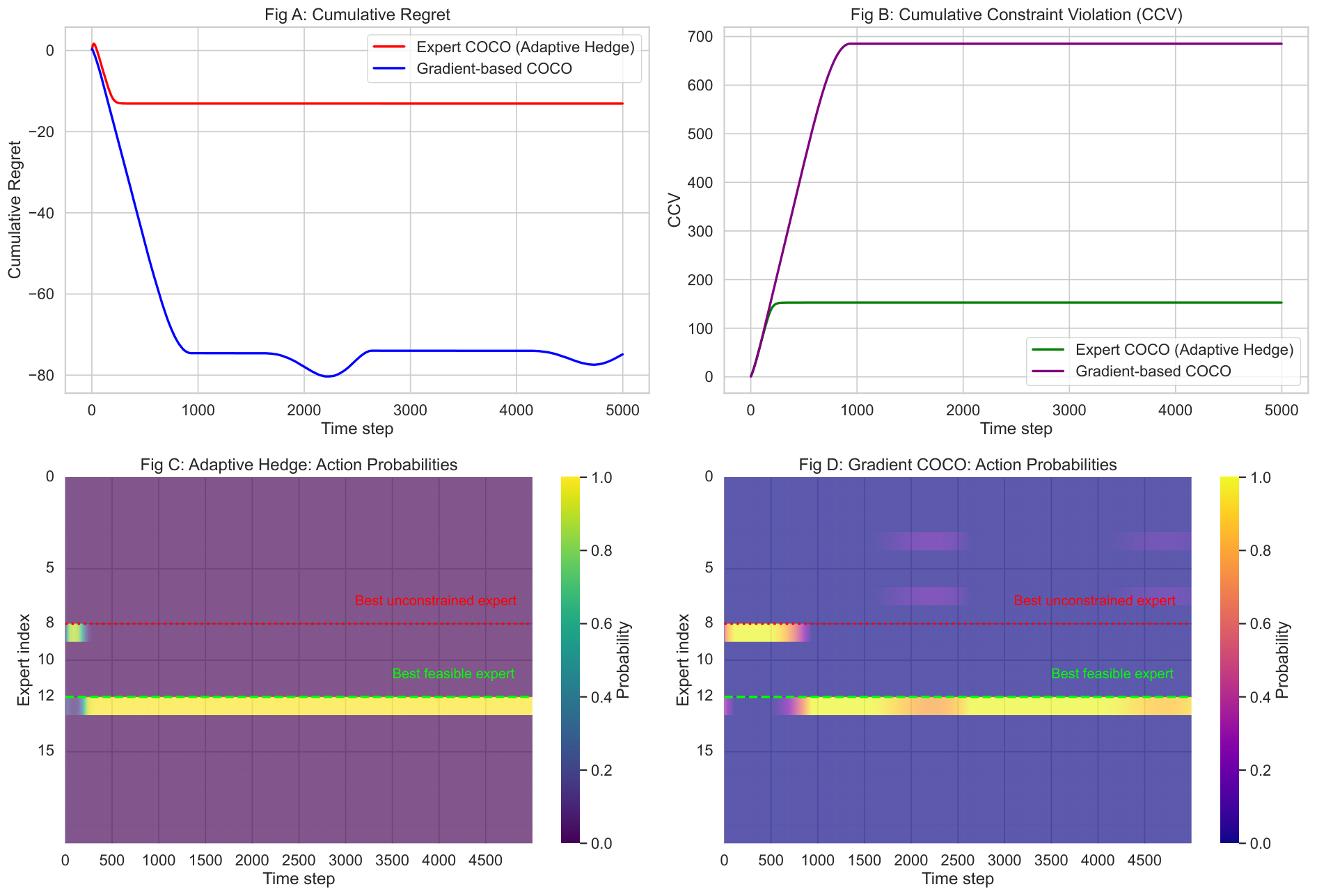
We consider the Constrained Expert problem on a synthetic dataset with $N=20$ experts over a horizon of length $T=5000$ . Two experts are designated as special: the best feasible expert, denoted by $\texttt{E}^{\star}$ , and the best unconstrained expert, denoted by $\texttt{UE}^{\star}$ . The expert $\texttt{E}^{\star}$ is feasible, with i.i.d. costs drawn from a distribution with mean $\bar{f}_{\texttt{E}^{\star}}=0.21$ , and zero constraint violation on all rounds, i.e., $\bar{g}_{\texttt{E}^{\star}}=0.0$ . In contrast, $\texttt{UE}^{\star}$ is infeasible, with i.i.d. costs and constraint violations having a smaller mean $\bar{f}_{\texttt{UE}^{\star}}=0.11$ and higher average constraint violation $\bar{g}_{\texttt{UE}^{\star}}=0.91$ , respectively. The remaining experts incur i.i.d. random costs with mean $\bar{f}=0.41$ plus a zero-mean periodic component over time, and their constraint violations are i.i.d. with mean $\bar{g}=0.6$ . Additionally, two more experts, $\texttt{DE}_{1}$ and $\texttt{DE}_{2}$ , distinct from both $\texttt{E}^{\star}$ and $\texttt{UE}^{\star}$ , are made feasible by setting their constraint violations to zero on all rounds. Table 2 summarizes the parameters used in the experiments. The experiments have been run on a quad-core CPU with 8 GB RAM. The source code has been made publicly available [Sinha, 2025].

Parameters for Experts Used in the Experiments Expert(s) Index Average cost Average constraint violation $\texttt{E}^{\star}$ $\#12$ $\bar{f}_{\texttt{E}^{\star}}=0.21$ $\bar{g}_{\texttt{E}^{\star}}=0.0$ $\texttt{UE}^{\star}$ $\#8$ $\bar{f}_{\texttt{E}^{\star}}=0.11$ $\bar{g}_{\texttt{E}^{\star}}=0.91$ $\texttt{DE}_{1},\texttt{DE}_{2}$ $\#3,\#6$ $\bar{f}_{\texttt{E}^{\star}}=0.41$ $\bar{g}_{\texttt{E}^{\star}}=0.0$ The rest $[20]\setminus\{3,6,8,12\}$ $\bar{f}_{\texttt{E}^{\star}}=0.41$ $\bar{g}_{\texttt{E}^{\star}}=0.6$

Table 2: Parameter settings for generating cost and constraint vectors for

N=20

experts.

Summary of the results.

Parts (A) and (B) of Figure 2 compare the performance of our proposed adaptive Hedge-based policy (Algorithm 1) with $\beta=0.75$ with that of the Online Gradient Descent (OGD)-based policy proposed by Sinha and Vaze [2024, Algorithm 1]. From the plots, it is evident that the proposed algorithm incurs significantly lower cumulative constraint violation (CCV) while maintaining a sub-linear regret.

To gain deeper insight into the working of the algorithms, parts (C) and (D) of Figure 2 show the relative frequency with which each expert is selected by our algorithm and the OGD-based policy, respectively. These plots clearly demonstrate that the adaptive Hedge-based policy quickly identifies the best feasible expert and predominantly selects it thereafter. In contrast, the OGD-based policy initially incurs a substantial amount of constraint violation by frequently selecting infeasible experts. Only after a considerable number of rounds does it converge to the best feasible expert and begin exploiting it consistently.

Figure 3 illustrates the trade-off between regret and cumulative constraint violation (CCV) for different values of the tuning parameter $\beta$ in the proposed policy. As $\beta$ increases from 0.6 to 0.9, the algorithm incurs lower CCV at the expense of higher regret. This behavior aligns with the theoretical performance guarantees established in Theorem 2.

Figure 3: Performance comparison for different values of

\beta

Beyond O~​(T)\tilde{O}(\sqrt{T}) Constraint Violation for Online Convex Optimization with Adversarial Constraints

Abstract

1 Introduction

Assumption 1 (Bounded Cost and Constraints).

Assumption 2 (Feasibility).

Goal:

Background and Our Contribution

Intuition for the results:

1.1 Prior work

2 Preliminaries: Adaptive Small-Loss Regret Bound for the Expert Problem

Theorem 1.

3 The Constrained Expert problem: Simplex Decision Set, Linear Cost, and Linear Constraint Functions

3.1 An Online Policy for the Constrained Expert Problem

Theorem 2.

3.2 Proof of Theorem 2

1. Bounding the CCV:

2. Bounding the Regret:

4 Convex Cost and Constraint functions

Assumption 3 (Convexity and Lipschitzness).

Definition 1 (Covering number).

Construction:

Feasibility:

Algorithm:

Analysis:

Theorem 3.

5 Convex and Smooth Cost and Constraint Functions

Theorem 4 (Orabona (2019), Theorem 4.25).

Assumption 4 (Convexity and Smoothness).

Algorithm and Analysis:

Theorem 5.

6 Conclusion

7 Acknowledgement

References

8 Appendix

8.1 On the Boundedness Assumption

8.2 Pseudocode for the Adaptive Hedge Policy

8.3 Proof of Theorem 1

8.4 Proof of Auxiliary Lemmas

Lemma 1 (A quadratic inequality).

Proof.

Lemma 2 (Bounding γ\gamma).

Proof.

8.5 Construction of a Minimal δ\delta-cover of the Decision Set 𝒳\mathcal{X}

8.6 Relaxing the Feasibility Assumption

Assumption 5 (Long-term Feasibility).

8.6.1 The Generalized Regret Decomposition Inequality

8.6.2 Convex and Smooth Cost and Constraints with Long-term Budget Constraints

Bounding the CCV:

Bounding the Regret:

Theorem 6.

8.7 Experiments

Problem instance:

Summary of the results.

Beyond $\tilde{O}(\sqrt{T})$ Constraint Violation for Online Convex Optimization with Adversarial Constraints

Lemma 2 (Bounding $\gamma$ ).

8.5 Construction of a Minimal $\delta$ -cover of the Decision Set $\mathcal{X}$