Refer to caption — Figure 1. We present the Anymate Dataset and a learning-based framework for automatic 3D object rigging. This dataset comprises 230K 3D assets with expert-crafted rigging and skinning information. Using this dataset, our framework learns to predict bone skeletons and skinning weights automatically from a given 3D mesh, allowing users to create realistic animations by manipulating the predicted skeleton.

Anymate: A Dataset and Baselines for Learning 3D Object Rigging

Conference: Special Interest Group on Computer Graphics and Interactive Techniques Conference Conference Papers ; August 10–14, 2025; Vancouver, BC, CanadaDOI: 10.1145/3721238.3730743ISBN: 979-8-4007-1540-2/2025/08CCS: Computing methodologies Animation

Yufan Deng Note: Equal contribution. The order of authorship was determined alphabetically. Work was done when Y. Deng and Y. Zhang were visiting students at Stanford University; they are currently with the Hong Kong University of Science and Technology. Affiliation: Stanford University, Stanford, USA , Yuhao Zhang Affiliation: Stanford University, Stanford, USA , Chen Geng Affiliation: Stanford University, Stanford, USA , Shangzhe Wu Note: Equal advising. Affiliation: Stanford University, Stanford, USA Affiliation: University of Cambridge, Cambridge, UK and Jiajun Wu Affiliation: Stanford University, Stanford, USA

2025

Abstract.

Rigging and skinning are essential steps to create realistic 3D animations, often requiring significant expertise and manual effort. Traditional attempts at automating these processes rely heavily on geometric heuristics and often struggle with objects of complex geometry. Recent data-driven approaches show potential for better generality, but are often constrained by limited training data. We present the Anymate Dataset, a large-scale dataset of 230K 3D assets paired with expert-crafted rigging and skinning information—70 times larger than existing datasets. Using this dataset, we propose a learning-based auto-rigging framework with three sequential modules for joint, connectivity, and skinning weight prediction. We systematically design and experiment with various architectures as baselines for each module and conduct comprehensive evaluations on our dataset to compare their performance. Our models significantly outperform existing methods, providing a foundation for comparing future methods in automated rigging and skinning. Code and dataset can be found at https://anymate3d.github.io/.

Keywords:

Data Driven Animation, Auto Rigging

1. Introduction

With rapid advances of immersive¹¹footnotetext: Equal contribution, alphabetical order. ^†Equal advising. media comes a growing demand for automated 3D content creation. 3D animation is essential nowadays across the entertainment industry, from game design and movie production to a wide range of AR/VR applications. Yet, producing realistic 3D animations remains one of the most labor-intensive tasks, often requiring enormous expert effort.

Creating an animation of a 3D object generally involves two steps. The first is to describe the desired motion using a set of sparse, interpretable motion handles, such as keypoints or bones—often referred to as a “rig.” The second step, known as “skinning,” then defines how the 3D object deforms densely according to the movement of these handles. Both steps require specialized expertise and meticulous effort to ensure realistic animation results.

In this paper, our goal is to develop a model that can efficiently and fully automatically turn a static 3D asset into an animatable version. To this end, we propose a learning-based auto-rigging system that generates a rig and the corresponding skinning mechanism from a given 3D mesh. This allows users to create realistic 3D animations by simply manipulating the underlying rig in an intuitive manner.

The key insight is to leverage existing large-scale animated 3D assets handcrafted by expert artists. Large-scale 3D data has proven crucial in training high-quality 3D generation models (Shi et al., 2023; Liu et al., 2024). Notably, the Objaverse datasets (Deitke et al., 2022; Deitke et al., 2024), aggregating over 10 million 3D assets from various public sources, have powered many recent state-of-the-art methods. However, prior efforts primarily use such assets for static 3D generation, neglecting the fact that many of these assets also come with valuable animation information skillfully crafted by the artists.

To train a learning-based model for 3D object rigging, we assemble a large-scale dataset of 230K rigged 3D assets curated from the Objaverse-XL Dataset (Deitke et al., 2024), each paired with artist-created rigging and skinning in a unified format, dubbed the Anymate Dataset. This dataset is 70 times larger than existing public rigging datasets, as summarized in Table 1, and contains a wide spectrum of 3D objects, ranging from humanoid and animal characters to animated everyday objects like furniture and machines.

Using the Anymate Dataset, we develop a learning-based framework that predicts a 3D bone skeleton and corresponding skinning weights fully automatically from any given 3D object mesh. This framework consists of three sequential modules for joint, connectivity, and skinning weight prediction. For each module, we design several architectures as strong baselines and provide a comprehensive set of evaluations and comparisons on the proposed dataset. These experiments show that the larger scale of training data significantly improves prediction results. Moreover, our proposed architectures demonstrate better scalability, outperforming existing methods by a considerable margin. The dataset, code, and pretrained weights will be publicly released to facilitate future research.

Our contributions are summarized as follows:

(1)

We introduce the Anymate Dataset consisting of 230K 3D assets with rigging and skinning information.
(2)

We develop a learning-based framework for automatic 3D object rigging and skinning.
(3)

We design a comprehensive set of baselines with a variety of architectures and provide thorough evaluations and comparisons on the proposed dataset, providing a reference point for future comparisons.

2. Related Work

2.1. 3D Object Rigging Datasets

Auto-rigging has traditionally been approached through geometry-based optimization. Hence, limited efforts were dedicated to collecting and open-sourcing large-scale rigging datasets before the recent rise of data-driven methods. Most of the existing public rigging datasets focus primarily on humanoid and animal characters, such as SMPL (Loper et al., 2015), DeformingThings4D (Li et al., 2021), Maximo (Adobe, 2024), Planet Zoo (Wu et al., 2022), Model Resource (Xu et al., 2019), and RaBit (Luo et al., 2023). The largest of these, Model Resource, contains only 3.3K assets. Our dataset consists of 230K assets—around 70x larger—which is crucial for training robust learning-based models. Table 1 compares the key features of these datasets.

Our Anymate Dataset is built upon the recently released Objaverse-XL Dataset (Deitke et al., 2024), which consists of over 10M 3D assets. The authors of (Li et al., 2024) also extract a set of 14K animated assets in Objaverse (Deitke et al., 2022), dubbed Objaverse-Animation. Unlike ours, this dataset is curated to train an implicit image-based model for object animation, offering no direct access to rigging and skinning information.

Table 1. 3D Object Rigging Datasets. Existing datasets are limited in both size and variety. In contrast, our Anymate Dataset is 70 times larger than the existing datasets with rigging.

Dataset	Size	Category	Rigging
DeformingThings4D (Li et al., 2021)	2.0K	humanoid, animal	✗
Objaverse-Animation (Li et al., 2024)	14K	generic	✗
SMPL (Loper et al., 2015)	0.2K	human	✓
Mixamo (Adobe, 2024)	0.1K	humanoid	✓
Planet Zoo (Wu et al., 2022)	0.25K	animal	✓
RaBit (Luo et al., 2023)	1.5K	humanoid	✓
Model Resource (Xu et al., 2020)	3.3K	humanoid, animal	✓
Anymate Dataset (ours)	230K	generic	✓

2.2. Skeleton-based Automatic 3D Object Rigging

Early auto-rigging methods, such as Pinocchio (Baran and Popović, 2007) and Avatar Reshaping (Feng et al., 2015), fit a template skeleton to a given mesh through optimization. This requirement of a template skeleton heavily limits the range of applicable objects, typically to humanoid or quadruped characters. Several works have explored data-driven approaches for rigging prediction (Xu et al., 2020; Xu et al., 2019; Ma and Zhang, 2023).

In particular, (Xu et al., 2019) uses a 3D convolution-based architecture that operates on voxelized shapes, whereas the follow-up works of RigNet (Xu et al., 2020) and Tarig (Ma and Zhang, 2023) replace it with graph neural networks that directly process mesh vertices. However, these models are all trained on small-scale datasets with less than 3K objects and often generalize poorly to complex objects, as shown in fig. 7.

Concurrent to our work, RigAnything (Liu et al., 2025) and MagicArticulate (Song et al., 2025) present auto-regressive rigging models learned from large-scale data. Compared to those works, we focus on presenting the dataset, benchmark, and a set of baseline methods for future comparison.

2.3. Non-skeletal Automatic 3D Object Rigging

There also exist works that achieve automatic rigging using representations other than skeleton. We summarize them as handle-based, cage-based, and neural-based methods.

Handle-based.

KeypointDeformer (Jakab et al., 2021) and DeepMetaHandles (Liu et al., 2021) pioneer the unsupervised learning of deformation handles. While being annotation-free, these methods often require datasets with minor deformations or aligned poses, which limits their applications to broader categories. In contrast, skeleton-based approaches benefit from large-scale artist-annotated ground truth for supervised learning. We have tried KeypointDeformer (Jakab et al., 2021) but find that instead of manipulating motion, handle-based methods focus on manipulating the mesh’s shape, i.e, adjusting an airplane’s wing length.

Cage-based.

Methods like Neural Cages (Yifan et al., 2020) offer promising approaches to learning rigging without large annotated datasets. However, they struggle with objects with complex hierarchical kinematic structures and large-scale deformations.

Neural-based.

Rigging methods with a neural representation (Aigerman et al., 2022; Qin et al., 2023) are promising for modeling complex motions like faces, but often require an extensive amount of observations under known poses for training. Moreover, it remains challenging to obtain an interpretable neural representation.

In summary, different rigging modalities serve distinct purposes. The skeleton-based approach benefits from large-scale annotated datasets, applies to diverse categories, and integrates seamlessly with traditional graphics pipelines. Other modalities excel in specific contexts, such as with aligned datasets or synthetic data.

2.4. Automatic Skinning

In 3D animation, artists usually need to paint skinning weights on a mesh to indicate how the vertices should deform in response to bone movement. Techniques like Linear Blend Skinning (LBS) (Magnenat et al., 1988) are then used to drive the mesh based on bone animations. Various geometric methods have been proposed to automatically determine skinning weights (Bang and Lee, 2018; Dionne and De Lasa, 2014; Dionne and de Lasa, 2013; Chen et al., 2021; Kavan and Sorkine, 2012; Jacobson et al., 2011; Song et al., 2024), such as using Laplacian energy (Jacobson et al., 2011) or geodesic distance (Dionne and de Lasa, 2013). However, these methods often struggle with objects of complex geometry.

Previous data-driven approaches have shown promise for better generality (Xu et al., 2020; Mosella-Montoro and Ruiz-Hidalgo, 2022; Ma and Zhang, 2023; Liu et al., 2019). Nevertheless, similar to rigging, previous methods either focus on specific categories and rely on templates (Liao et al., 2024) or train on limited datasets (Xu et al., 2020; Mosella-Montoro and Ruiz-Hidalgo, 2022).

3. Anymate Dataset

To learn 3D object auto-rigging, a sizable collection of examples is essential. We introduce the Anymate Dataset, a large-scale dataset of manually crafted animated 3D objects, building upon the existing Objaverse-XL Dataset (Deitke et al., 2024). In the following, we first give an overview of the representation for 3D object animation, and then describe the procedures used to build the Anymate Dataset.

3.1. Preliminary: 3D Object Animation

When artists create an animation of a 3D object, two key components are typically required: rigging and skinning. The former establishes a set of sparse, interpretable handles that serve as a scaffold to outline the intended motion. The latter, in turn, defines how the 3D object should deform densely in response to the motion scaffold. In modern computer graphics, the rig is often represented by a skeleton of bones, and the skinning is usually defined by weights associating mesh vertices to these underlying bones.

Concretely, given a 3D mesh with vertices denoted by $\mathbf{V}\subset\mathbb{R}^{3}$ , we first define a set of bones, indexed by $b=1,...,B$ . Each bone is an oriented line segment specified by a pair of head and tail joints $\mathbf{J}_{b}^{\text{head}},\mathbf{J}_{b}^{\text{tail}}\in\mathbb{R}^{3}$ in the world coordinate space. In practice, these bones are typically connected via shared joints, forming a kinematic tree structure.

To animate the object, we then deform each vertex $\mathbf{V}_{i}$ of the mesh according to the poses $\xi$ of these bones via the Linear Blend Skinning (LBS) equation (Magnenat et al., 1988; Lewis et al., 2000):

(1)		$\displaystyle\mathbf{V}_{i}^{\prime}(\xi)=\left(\sum_{b=1}^{B}w_{i,b}G_{b}(\xi)G_{b}(\xi^{*})^{-1}\right)\mathbf{V}_{i},$
(1)		$\displaystyle G_{1}=g_{1},~~G_{b}=G_{\pi(b)}\circ g_{b},~~g_{b}(\xi_{b})\in SE(3).$

Here, $\xi=\{\xi_{1},...,\xi_{B}\}$ denotes the poses of the bones in their local coordinate frames, and $\xi^{*}$ denotes the rest pose, which can be derived from the joint locations $\mathbf{J}_{b}^{\text{head}}$ and $\mathbf{J}_{b}^{\text{tail}}$ (see the supp. mat.). $G$ stands for the global transformation matrix after composing all the local transformations $g_{b}$ along the kinematic chain. $\pi(b)$ retrieves the index of the parent of bone $b$ in the kinematic tree. $w_{i,b}$ is the skinning weight of vertex $\mathbf{V}_{i}$ with respect to bone $b$ . Essentially, for each bone $b$ , vertex $\mathbf{V}_{i}$ in the world coordinate frame is first transformed to the local coordinate frame of the bone following the inverse kinematic chain $G_{b}^{-1}$ , and then reposed together with the bone following the forward kinematic chain $G_{b}$ . The final position of the vertex $\mathbf{V}_{i}^{\prime}$ is the sum of transformations from all bones weighted by $w_{i,b}$ .

Therefore, to animate a mesh, we need a set of bones $\mathcal{B}$ , each specified by a pair of joints $\mathcal{B}_{b}=(\mathbf{J}_{b}^{\text{head}},\mathbf{J}_{b}^{\text{tail}})$ , and a function $\mathcal{S}$ that returns the skinning weights for a given point on the surface. The goal of our model is thus to predict these bones and skinning weights from a given mesh.

3.2. Dataset Processing

To train such a model, we prepare a large dataset of rigged 3D objects. Our dataset contains 230K 3D assets of common objects from the Objaverse-XL dataset (Deitke et al., 2024). Each asset comes with a 3D mesh, a bone skeleton, and skinning weights for each mesh vertex in a unified format.

Filtering.

Objaverse-XL provides links to over 10 million 3D assets from various public sources in various formats. We identify the assets that potentially contain rigging and skinning information with a file format of .fbx, .dae, .gltf, or .glb. While Objaverse-XL reports 438K objects with armatures, we find only 256K that are still publicly available. We then filter the assets, retaining roughly 200K with a vertex count of $128<|\mathbf{V}|<65,535$ and a bone count of $8<|\mathcal{B}|<64$ . Fig. 2 gives an illustration of the statistics. After this, we eliminate redundant data based on skeleton similarity. Next, we remove assets where most of the skeleton ( $>70\%$ ) lies outside the mesh. Many assets contain animation information, which is used to augment the dataset. We use no more than three extra key-frame poses from the same asset. After augmentation, we unify the data format and fix bones and joints. More details can be found in the supp. mat.

Pre-processing.

We load these assets into Blender¹¹ 1 https://www.blender.org/ and extract the mesh, armature (bones), and skinning weights. For training efficiency, we resample 8,192 points on the mesh, and recompute their skinning weights using barycentric interpolation based on the original annotated skinning weights at the vertices. Finally, for each asset, we export the original mesh in a unified .obj format, as well as the resampled point clouds and the corresponding bone locations and skinning weights.

Dataset Statistics.

The final dataset contains $230,716$ assets. We randomly select 5.6K instances as the test set (Anymate-test), and use the rest 225K for training (Anymate-train). To facilitate efficient ablation experiments, we also construct a smaller 14K training set (Anymate-small) with a subset of training instances that are included in the original Objaverse 1.0 Dataset (Deitke et al., 2022), which is likely of higher quality.

4. Learning to Rig 3D Objects

Using the Anymate Dataset, we train learning-based models to predict bone skeleton and skinning weights from a given 3D object mesh. These allow users to create 3D animations of the object by simply manipulating the skeleton.

We divide this task into three sequential sub-tasks: joint prediction, connectivity prediction, and skinning weight prediction, as outlined in Fig. 3. Starting with an input 3D mesh, we first use an encoder $f_{\text{enc}}$ to extract shape features, which are then fed into the three subsequent prediction modules. The first module $f_{\text{joint}}$ predicts a set 3D joints. The second module $f_{\text{conn}}$ then connects these joints into bones by predicting binary connectivity for each pair of joints, forming a skeleton. Finally, the skinning module $f_{\text{skin}}$ estimates the skinning weight between each mesh vertex and each bone, based on the constructed skeleton. For each sub-task, we experiment with various architectures as baselines and conduct evaluations on our Anymate Dataset, comparing against previous methods.

In the following, we first introduce the shape encoder (section 4.1) shared across all prediction modules, and then discuss each individual module (sections 4.2, 4.3 and 4.4), followed by visual results generated using the predictions (section 4.5).

4.1. Shape Encoding

Given a 3D mesh, we first uniformly resample $8,192$ points across its surface and extract shape latent features $\phi$ using an encoder $f_{\text{enc}}$ . We experiment with two popular transformer-based point cloud encoders, Michelangelo (Zhao et al., 2024) and Point-BERT (Yu et al., 2022). Michelangelo trains a perceiver-based transformer with learnable query tokens and several self-attention blocks. Point-BERT trains a discrete Variational Auto-Encoder (dVAE) which first maps a point cloud into a set of patch tokens and subsequently mixes them via a transformer. Both models encode the point cloud into a set of feature tokens (257 and 513 respectively). In our experiments, we load the pre-trained weights from existing models and fine-tune them with each subsequent prediction module individually. Specifically, we load the Michelangelo model pre-trained on the ShapeNet Dataset (50K) (Chang et al., 2015), and the Point-BERT model pre-trained on the Cap3D Dataset (660K) (Luo et al., 2024) released by PointLLM (Xu et al., 2024b), as Cap3D is also derived from Objaverse (Deitke et al., 2022).

4.2. Joint Prediction

After obtaining the shape latent $\phi$ , the joint prediction module $f_{\text{joint}}$ predicts a set of joints $\hat{\mathcal{J}}=f_{\text{joint}}(\phi)=\{\hat{\mathbf{J}}_{k}\}_{k=1}^{K}$ , where each joint $\hat{\mathbf{J}}_{k}\in\mathbb{R}^{3}$ is a 3D coordinate in world space, and the number of joints $K$ may vary across instances.

4.2.1. Architectures

We explore three types of architectures for $f_{\text{joint}}$ : regression-based, diffusion-based, and volume-based.

Regression-based.

A regression-based model is perhaps the most intuitive approach for joint prediction, which simply regresses a set of 3D coordinates from the extracted shape features and can be directly supervised by the ground-truth joints during training. However, there are two unique features that make our joint prediction task different from typical regression problems: (1) the number of target joints varies across instances, and (2) the order of the joints is immaterial at this stage²² 2 Although an order could technically be established based on the skeleton, inconsistencies may arise across instances created by different artists.. To address these challenges, we design a transformer-based architecture (Jaegle et al., 2021; Vaswani et al., 2017), which is permutation-equivariant and has proven to be highly scalable, followed by a clustering step (Ester et al., 1996).

The architecture is illustrated in Fig. 4(a). Specifically, we use a single-layer perceiver-based transformer (Jaegle et al., 2021) with a fixed number of $K_{\text{pred}}=96$ learnable query tokens and the shape latent $\phi$ as key and value tokens, followed by a $3$ -layer MLP to produce $K_{\text{pred}}$ 3D joint locations $\hat{\mathcal{J}}$ . We supervise the model directly using a standard Chamfer Distance between the predicted joints and the ground-truth joints.

Since the number of GT joints ${K_{\text{gt}}}$ varies across training instances, we cluster the raw predicted joints using the technique of (Ester et al., 1996) and use the cluster centers as the final output.

Diffusion-based.

Another commonly used architecture for point set generation is diffusion-based models (Sohl-Dickstein et al., 2015), which tend to excel with large-scale training. However, unlike most existing work that focuses either on generating dense point clouds with high geometric redundancy (Luo and Hu, 2021; Nichol et al., 2022; Huang et al., 2024) or on producing a fixed set of semantic keypoints like human poses (Zhou et al., 2023; Xu et al., 2024a), our model is designed to predict salient joints for animation which may vary across instances.

Following DDPM (Ho et al., 2020), the forward diffusion process injects noise $\bm{\epsilon}_{t}=\{\bm{\epsilon}_{k,t}\}_{k=1}^{K}$ independently to the GT joints $\mathcal{J}_{0}=\{\mathbf{J}_{k,0}\}_{k=1}^{K}$ at a time step $t\in\left[1,T\right]$ :

\mathbf{J}_{k,t}=\sqrt{\overline{\alpha}_{t}}\mathbf{J}_{k,0}+\sqrt{1-\overline{\alpha}_{t}}\bm{\epsilon}_{k,t},\quad\bm{\epsilon}_{k,t}\sim\mathcal{N}(\mathbf{0},\,\mathbf{I}),

where $\overline{\alpha}_{t}$ signifies the noise schedule. We then train a denoiser $\bm{\epsilon}_{\theta}(\mathcal{J}_{t},t\mid\phi)$ that learns to predict the noise from the noised joints $\mathcal{J}_{t}=\{\mathbf{J}_{k,t}\}$ conditioned on the shape latent $\phi$ , using the loss:

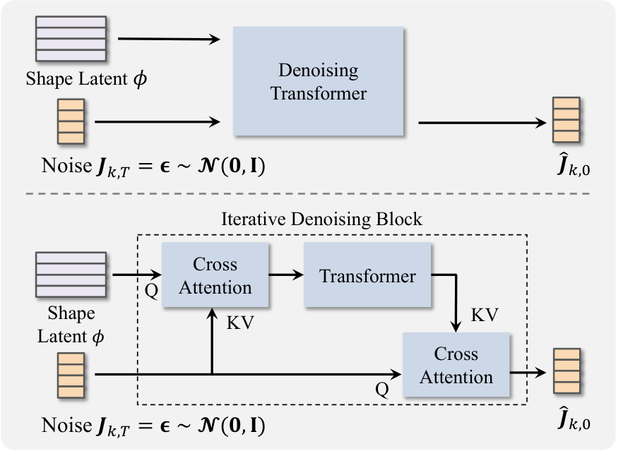
L_{\text{diff}}=\mathbb{E}_{t,\mathcal{J}_{0},\bm{\epsilon}_{t}}\left[\|\bm{\epsilon}_{t}-\bm{\epsilon}_{\theta}(\mathcal{J}_{t},t\mid\phi)\|_{2}^{2}\right].

We implement the denoiser using a permutation-equivariant transformer architecture with two variations, as illustrated in Fig. 4(b):

(1)

Concatenation-based model inspired by Point-E (Nichol et al., 2022), where the noisy joints $\mathbf{J}_{k,t}$ are concatenated with the shape latent $\phi$ before passing through a transformer;
(2)

Cross-attention-based model inspired by Point-Infinity (Huang et al., 2024), where cross-attention and transformer modules iterate across two branches, between the noisy joints $\mathbf{J}_{k,t}$ and the shape latent $\phi$ .

At inference time, we use a DDIM (Song et al., 2021) sampler to generate a set of joints $\hat{\mathcal{J}}_{0}$ from Gaussian noise. This transformer-based diffusion architecture allows users to specify an arbitrary number of joints at varying levels of granularity during inference by adjusting the shape of the initial noisy point cloud, as demonstrated in the supp. mat.

Volume-based.

The final option we explore is a dense volume-based model, where the task is framed as predicting the probably of a point in space being near a joint. To this end, we experiment with two commonly used 3D field representations, an implicit neural field (Mildenhall et al., 2021) and a tri-plane representation (Chan et al., 2022), as illustrated in Fig. 4(c).

For the implicit neural field, we follow Michelangelo (Zhao et al., 2024) and implement it using a perceiver-based transformer. It takes in a set of 3D coordinates $\mathbf{x}_{i}$ conditioned on the shape latent $\phi$ , and predicts a scalar $\sigma(\mathbf{x}_{i})$ indicating the probability that a joint is nearby. For direct supervision, we apply a 3D Gaussian kernel to each GT joint with a standard deviation $\gamma$ ( $=2\ \mathrm{voxel}$ ) and take the maximum response across all joints at each 3D location. At inference time, we first extract a $64^{3}$ voxel grid of joint probability scores from the implicit field and apply a threshold to obtain a set of activated grid points. We then apply the same clustering technique (Ester et al., 1996) to group these points into clusters.

For the tri-plane representation, we follow the implementation of EG3D (Chan et al., 2022) with a StyleGAN2 generator (Karras et al., 2020) conditioned on the shape latent. We then use a similar procedure to extract keypoints from the tri-planes.

4.2.2. Existing Methods

We also evaluate two existing auto-rigging methods on our dataset, Pinocchio (Baran and Popović, 2007) and RigNet (Xu et al., 2020). Pinocchio relies on predefined template skeletons (humanoid or quadruped), and fit a template to a given mesh via optimization. RigNet proposes a learning-based system similar to ours, but uses primarily Graph Neural Networks. We adopt the official public implementation for both methods, and train the RigNet model on our larger Anymate Dataset. We also compare with two commercial auto-rigging tools, Maya (Autodesk, 2024) and Animate Anything (World, 2024), qualitatively in section 4.5.

4.2.3. Quantitative Results

Table 2. Quantitative Evaluation of Joint Prediction. Our proposed architectures scale more effectively with larger training data, outperforming existing methods by a significant margin.

trained on Anymate-small (14K)
Model	CD $\downarrow$	EMD $\downarrow$	Training Time
Pinocchio (Baran and Popović, 2007)	0.198	0.659	-
RigNet (Xu et al., 2020)	0.094	0.131	16h
Mich-Regress	0.099	0.124	20h
Mich-Diff_Concat	0.142	0.175	26h
Mich-Diff_Cross	0.128	0.160	47h
Mich-Vol_Implicit	0.147	0.127	33h
Mich-Vol_TriPlane	0.198	0.186	20h
Bert-Regress	0.091	0.113	11h
Bert-Diff_Concat	0.147	0.177	65h
Bert-Diff_Cross	0.137	0.167	37h
Bert-Vol_Implicit	0.123	0.126	29h
Bert-Vol_TriPlane	0.192	0.171	19h
trained on Anymate-train (225K)
RigNet (Xu et al., 2020)	0.089	0.127	114h
Bert-Regress	0.077	0.098	79h
Mich-Diff_Cross	0.083	0.104	151h

For a comprehensive analysis of different architectures, we first train 10 models on the Anymate-small set, exhausting all combinations of the 2 shape encoders and 5 prediction architectures. We then evaluate these models and the existing methods (RigNet and Pinocchio) on the Anymate-test set. For quantitative evaluation, we compute two standard metrics, Chamfer Distance (CD) and Earth Mover’s Distance (EMD), both computed between the predicted and the annotated joints (see supp. mat.).

The results are summarized in Table 2. Among the proposed architectures trained on Anymate-small, Bert-Regress outperforms the two existing methods. We select two architectures for training on the full Anymate-train set: Bert-Regress, and Mich-Diff_Cross. The regression-based model performs best on the Anymate-small subset, while the diffusion-based model has the potential for scaling with larger training data. As shown in Table 2, the performance of the model improves as training set increases from 14K to 225K, in particular, from 0.091 to 0.077 for Mich-Diff_Cross. Despite comparable performance, compared to the regression-based models, the diffusion-based model offers the flexibility for a user to specify an arbitrary number of target joints, but requires a more time-consuming iterative inference procedure. In comparison, the classic geometric method, Pinocchio (Baran and Popović, 2007), performs significantly worse. RigNet (Xu et al., 2020) scales poorly with the larger dataset, leading to degraded performance. We also report the training time in terms of GPU hours on a L40S GPU for Anymate-small training and on eight TITANRTX GPUs for Anymate-train training. More analysis is provided in the supp. mat.

4.3. Connectivity Prediction

After obtaining a set of joints $\{\hat{\mathbf{J}}_{k}\}_{k=1}^{K}$ , the second module $f_{\text{conn}}$ predicts connectivity between the joints to establish a bone skeleton. Specifically, it takes the predicted joints and the shape latent $\phi$ as inputs, and predicts a connectivity matrix $\hat{\mathbf{C}}=f_{\text{conn}}(\hat{\mathcal{J}},\phi)\in\mathbb{R}^{K\times K}$ , where each element $\hat{c}_{i,j}$ indicates the probability that $\hat{\mathbf{J}}_{i}$ and $\hat{\mathbf{J}}_{j}$ are connected by a bone, with $\hat{\mathbf{J}}_{i}$ as the head joint and $\hat{\mathbf{J}}_{j}$ as the tail joint.

We train the model using the ground-truth joints $\{\mathbf{J}_{k}\}_{k=1}^{K}$ as input and compute binary cross entropy between the predicted and ground-truth connectivity matrices, $\hat{\mathbf{C}}$ and $\mathbf{C}$ . The GT matrix $\mathbf{C}\in\{0,1\}^{K\times K}$ can be generated from the annotated bones in the training assets. During inference, the trained model is used to infer the connectivity of the predicted joints $\{\hat{\mathbf{J}}_{k}\}_{k=1}^{K}$ .

In practice, Blender only allows each bone to have at most one parent bone. This implies that each joint can only serve as the tail joint of either one single bone or none (i.e., a root joint), meaning the sum of each column of the GT connectivity matrix $\mathbf{C}$ is either 1 or 0 (root). Therefore, if a joint $\mathbf{J}_{i}$ is a root joint, we assign the $(i,i)$ entry of $\mathbf{C}$ to 1, i.e., $c_{i,i}=1$ , while keeping the rest of the column as 0. At inference time, we can exploit this fact and simply take the argmax of each column of the predicted connectivity matrix $\hat{\mathbf{C}}$ to identify root joints or retrieve the head joints. This enables us to construct a kinematic chain for animation.

4.3.1. Architectures

We design two architectures to predict this connectivity matrix $\hat{\mathbf{C}}$ given a set of joints $\{\mathbf{J}_{k}\}_{k=1}^{K}$ conditioned on the shape latent $\phi$ : a token-conditioned architecture and a two-branch architecture, as illustrated in Fig. 5.

Token-conditioned.

Given the input joint coordinates, this model first applies positional encoding and extracts embeddings via a linear layer. These joint embeddings together with the shape latent $\phi$ go through a transformer to obtain a set of per-joint feature tokens $\{\psi_{k}\}$ . Each token $\psi_{k}$ is then concatenated with a (shared) learnable ‘head’ token $\psi^{\text{head}}$ and a (shared) learnable ‘tail’ token $\psi^{\text{tail}}$ , and goes through two separate MLPs, generating a pair of head-conditioned and tail-conditioned tokens $\psi_{k}^{\text{head}}$ and $\psi_{k}^{\text{tail}}$ . Finally, we simply compute the dot product between two sets of tokens $\{\psi_{k}^{\text{head}}\}$ and $\{\psi_{k}^{\text{tail}}\}$ to obtain the output matrix $\hat{\mathbf{C}}$ .

Two-branch.

Instead of conditioning on ‘head’ and ‘tail’ tokens, The two-branch model processes the joint embeddings through two independent transformer branches, after incorporating the shape latent via cross attention. Similarly, the final matrix $\hat{\mathbf{C}}$ is obtained by taking the dot product between the two sets of output tokens from each branch.

4.3.2. Existing Methods

We compare our models with the bone prediction module of RigNet (Xu et al., 2020) on our dataset. Rather than using the dot product, they directly feed in each pair of joints to an MLP and predict their connectivity, which is less computationally efficient ( $O(K^{2})$ ). Furthermore, they use a separate network to predict the probability of a joint being a root. In comparison, our models are more efficient by directly obtaining a connectivity matrix via a dot product.

Table 3. Quantitative Evaluation of Connectivity Prediction. Despite overfitting on the smaller training set, our proposed architectures scale effectively with larger training data.

trained on Anymate-small (14K)
Model	Precision $\uparrow$	Recall $\uparrow$	Training Time
RigNet (Xu et al., 2020)	60.6%	57.9%	8h
Mich-Token	58,0%	55.8 %	21h
Mich-2Branch	60.5%	58.5%	19h
Bert-Token	59.3%	57.2 %	15h
Bert-2Branch	61.6%	59.7%	12h
trained on Anymate-train (225K)
RigNet (Xu et al., 2020)	47.9%	50.4%	51h
Bert-2Branch	84.6%	83.5%	76h

4.3.3. Quantitative Results

Similar to joint evaluation, we evaluate all architecture combinations on Anymate-small, and train the top performing models on the full Anymate-train set. We report two standard metrics for comparison: Precision and Recall.

The results are summarized in Table 3. On Anymate-small, we in fact observe overfitting for all of our models, whereas RigNet performs reasonably well. However, on the full Anymate-train set, we observe the opposite: RigNet severely underfits potentially due to a limited model size, whereas our proposed architectures scale well with the larger dataset, outperforming RigNet by a significant margin. Additionally, the two-branch model tends to perform better than the token-conditioned model.

4.4. Skinning Weight Prediction

After obtaining the bones $\mathcal{B}$ , the final step is to predict the skinning weights $\hat{\mathbf{W}}_{i}=f_{\text{skin}}(\mathbf{V}_{i}\mid\mathcal{B},\phi)\in\mathbb{R}^{B}$ of each vertex $\mathbf{V}_{i}$ with respect to the bones, where $B=|\mathcal{B}|$ denotes the number of bones. In practice, our model takes in the joint locations $\mathbf{J}$ of the bones, and for efficiency, processes a set of points in a batch using a transformer architecture, producing a skinning weight matrix $\hat{\mathbf{W}}\in\mathbb{R}^{|\mathbf{V}|\times B}$ . For training, we use the resampled point clouds explained in section 3.2 together with the annotated bones as inputs, and compute the cosine similarity loss against the ground-truth skinning weights $\mathbf{W}$ (see supp. mat. for details). During inference, we can infer the skinning weights of the original mesh vertices over the predicted bones.

4.4.1. Architectures

We experiment with two architectures illustrated in Fig. 6.

Concatenation-based.

This model simply concatenates the point embeddings with the bone embeddings and shape latent $\phi$ , and mixes these embeddings to generate two set of token features: per-point tokens $\{\phi^{\text{point}}_{i}\}_{i=1}^{|\mathbf{V}|}$ and per-bone tokens $\{\phi^{\text{bone}}_{b}\}_{b=1}^{B}$ . Reusing the dot product trick in connectivity prediction followed by a softmax over all bones, we obtain a skinning weight matrix $\hat{\mathbf{W}}$ .

Cross-attention-based.

The second variant stacks two consecutive cross-attention layers. The per-point tokens $\{\phi^{\text{point}}_{i}\}_{i=1}^{|\mathbf{V}|}$ and per-bone tokens $\{\phi^{\text{bone}}_{b}\}_{b=1}^{B}$ is generated by passing the cross-attention layers. Finally, the skinning weight matrix $\hat{\mathbf{W}}$ is obtained via a dot product followed by a softmax.

4.4.2. Existing Methods

We compare against RigNet (Xu et al., 2020) as well as a traditional geometric method, GeoVoxel (Dionne and de Lasa, 2013). RigNet uses a graph neural network based architecture and only predicts the skinning weights with respect to the five nearest bones. In practice, we found this often insufficient, in particular with erroneous joint predictions. We train and evaluate RigNet on our proposed dataset using the official implementation and the same hyper-parameters. GeoVoxel calculates skinning weights simply based on the geodesic distance after voxelization. We evaluate GeoVoxel on our test set using the implementation from Maya (Autodesk, 2024).

Table 4. Quantitative Evaluation of Skinning Weight Prediction. Our proposed architectures scale effectively with larger training data, outperforming GeoVoxel (Dionne and de Lasa, 2013) and RigNet (Xu et al., 2020).

Model	CE $\downarrow$	Cos $\uparrow$	MAE $\downarrow$	Train Time
GeoVoxel	3.569	0.407	0.056	-
trained on Anymate-small (14K)
RigNet	1.573	0.671	0.031	11h
Mich-Concat	1.169	0.754	0.029	41h
Mich-Cross	1.270	0.766	0.026	21h
Bert-Concat	1.148	0.768	0.027	53h
Bert-Cross	1.134	0.801	0.025	32h
trained on Anymate-train (225K)
RigNet	1.521	0.693	0.028	49h
Bert-Cross	0.741	0.915	0.014	83h

4.4.3. Quantitative Results

Similarly, we train the models on both the Anymate-small and Anymate-train sets, and evaluate on the Anymate-test set. We report three metrics: Cross Entropy (CE), Cosine Similarity (Cos), and Mean Absolute Error (MAE).

The results are summarized in Table 4. Overall, GeoVoxel performs poorly on our test set, serving as a purely geometry-based lower-bound. Our proposed architectures scale well with the larger training set, outperforming the baselines by a significant margin. In contrast, little improvement is observed with RigNet as the training data size increases. Among our proposed architectures, Bert-Cross achieves the best results.

4.5. Visual Results

After all individual modules have been trained, we can run inference on any new test mesh and obtain the skeleton and skinning weights automatically in less than a minute. With these predictions, we can easily animate the object by manipulating the predicted skeleton, as visualized in Fig. 8 and Fig. 7 . For all visualizations, we use the best-performing model variants for inference, namely, Mich-Regress (joint), Bert-2Branch (connectivity), and Bert-Cross (skinning).

We compare our results against the previous method, RigNet (Xu et al., 2020), and two commercial auto-rigging tools, Maya (Autodesk, 2024) and Animate Anything (World, 2024). Maya only supports fitting a humanoid skeleton to the input mesh and generalizes poorly to non-humanoid objects. Animate Anything, on the other hand, classifies the object into one of a few categories and fits a category-specific skeleton. Both tools produce inaccurate skeletons for complex geometries, resulting in unrealistic animations. For a fair comparison, we retrain the RigNet model on our full dataset. However, it still generalizes poorly to challenging instances. In comparison, our model predicts highly accurate bone skeleton and skinning weights, enabling realistic animations.

5. Conclusions

We present the Anymate Dataset, the largest object rigging dataset to date, containing 230K 3D assets with rigging and skinning information. Using this dataset, we proposed an effective learning-based auto-rigging framework, with three modules for joint, connectivity, and skinning prediction. For each module, we carefully designed a set of baselines and thoroughly evaluated their performance using the proposed dataset. Experiment results have demonstrated that our proposed baselines scale effectively with the larger training data, outperforming previous methods and existing commercial auto-rigging tools, and provide a reference point for future research in data-driven auto-rigging.

Acknowledgements.

This work is in part supported by ONR YIP N00014-24-1-2117, NSF RI #2211258 and #2338203, the Stanford Institute for Human-Centered AI (HAI), the Stanford Center for Integrated Facility Engineering (CIFE), and Meta.

References

Adobe (2024) Adobe. 2024. Mixamo. https://www.mixamo.com/.
Aigerman et al. (2022) Noam Aigerman, Kunal Gupta, Vladimir G Kim, Siddhartha Chaudhuri, Jun Saito, and Thibault Groueix. 2022. Neural jacobian fields: Learning intrinsic mappings of arbitrary meshes. arXiv preprint arXiv:2205.02904 (2022).
Autodesk (2024) Autodesk. 2024. Maya. https://www.autodesk.com/products/maya/.
Bang and Lee (2018) Seungbae Bang and Sung-Hee Lee. 2018. Spline interface for intuitive skinning weight editing. ACM TOG 37, 5 (2018), 1–14.
Baran and Popović (2007) Ilya Baran and Jovan Popović. 2007. Automatic rigging and animation of 3d characters. ACM TOG 26, 3 (2007), 72–es.
Chan et al. (2022) Eric R Chan, Connor Z Lin, Matthew A Chan, Koki Nagano, Boxiao Pan, Shalini De Mello, Orazio Gallo, Leonidas J Guibas, Jonathan Tremblay, Sameh Khamis, et al. 2022. Efficient geometry-aware 3d generative adversarial networks. In CVPR. 16123–16133.
Chang et al. (2015) Angel X Chang, Thomas Funkhouser, Leonidas Guibas, Pat Hanrahan, Qixing Huang, Zimo Li, Silvio Savarese, Manolis Savva, Shuran Song, Hao Su, et al. 2015. Shapenet: An information-rich 3d model repository. arXiv preprint arXiv:1512.03012 (2015).
Chen et al. (2021) Xu Chen, Yufeng Zheng, Michael J Black, Otmar Hilliges, and Andreas Geiger. 2021. Snarf: Differentiable forward skinning for animating non-rigid neural implicit shapes. In ICCV. 11594–11604.
Deitke et al. (2024) Matt Deitke, Ruoshi Liu, Matthew Wallingford, Huong Ngo, Oscar Michel, Aditya Kusupati, Alan Fan, Christian Laforte, Vikram Voleti, Samir Yitzhak Gadre, et al. 2024. Objaverse-XL: A universe of 10m+ 3d objects. NeurIPS 36 (2024).
Deitke et al. (2022) Matt Deitke, Dustin Schwenk, Jordi Salvador, Luca Weihs, Oscar Michel, Eli VanderBilt, Ludwig Schmidt, Kiana Ehsani, Aniruddha Kembhavi, and Ali Farhadi. 2022. Objaverse: A Universe of Annotated 3D Objects. arXiv preprint arXiv:2212.08051 (2022).
Dionne and de Lasa (2013) Olivier Dionne and Martin de Lasa. 2013. Geodesic voxel binding for production character meshes. In SIGGRAPH. 173–180.
Dionne and De Lasa (2014) Olivier Dionne and Martin De Lasa. 2014. Geodesic binding for degenerate character geometry using sparse voxelization. IEEE TVCG 20, 10 (2014), 1367–1378.
Ester et al. (1996) Martin Ester, Hans-Peter Kriegel, Jorg Sander, Xiaowei Xu, et al. 1996. A density-based algorithm for discovering clusters in large spatial databases with noise.. In KDD, Vol. 96. 226–231.
Feng et al. (2015) Andrew Feng, Dan Casas, and Ari Shapiro. 2015. Avatar reshaping and automatic rigging using a deformable model. In SIGGRAPH. 57–64.
Ho et al. (2020) Jonathan Ho, Ajay Jain, and Pieter Abbeel. 2020. Denoising diffusion probabilistic models. In NeurIPS, Vol. 33. 6840–6851.
Huang et al. (2024) Zixuan Huang, Justin Johnson, Shoubhik Debnath, James M Rehg, and Chao-Yuan Wu. 2024. PointInfinity: Resolution-Invariant Point Diffusion Models. In CVPR. 10050–10060.
Jacobson et al. (2011) Alec Jacobson, Ilya Baran, Jovan Popovic, and Olga Sorkine. 2011. Bounded biharmonic weights for real-time deformation. ACM TOG 30, 4 (2011), 78.
Jaegle et al. (2021) Andrew Jaegle, Felix Gimeno, Andy Brock, Oriol Vinyals, Andrew Zisserman, and Joao Carreira. 2021. Perceiver: General perception with iterative attention. In ICML. 4651–4664.
Jakab et al. (2021) Tomas Jakab, Richard Tucker, Ameesh Makadia, Jiajun Wu, Noah Snavely, and Angjoo Kanazawa. 2021. Keypointdeformer: Unsupervised 3d keypoint discovery for shape control. In CVPR. 12783–12792.
Karras et al. (2020) Tero Karras, Samuli Laine, Miika Aittala, Janne Hellsten, Jaakko Lehtinen, and Timo Aila. 2020. Analyzing and Improving the Image Quality of StyleGAN. In CVPR.
Kavan and Sorkine (2012) Ladislav Kavan and Olga Sorkine. 2012. Elasticity-inspired deformers for character articulation. ACM TOG 31, 6 (2012), 1–8.
Lewis et al. (2000) J. P. Lewis, Matt Cordner, and Nickson Fong. 2000. Pose space deformation: a unified approach to shape interpolation and skeleton-driven deformation. In SIGGRAPH.
Li et al. (2024) Ruining Li, Chuanxia Zheng, Christian Rupprecht, and Andrea Vedaldi. 2024. Puppet-Master: Scaling Interactive Video Generation as a Motion Prior for Part-Level Dynamics. arXiv preprint arXiv:2408.04631 (2024).
Li et al. (2021) Yang Li, Hikari Takehara, Takafumi Taketomi, Bo Zheng, and Matthias Nießner. 2021. 4dcomplete: Non-rigid motion estimation beyond the observable surface. In ICCV. 12706–12716.
Liao et al. (2024) Zhouyingcheng Liao, Vladislav Golyanik, Marc Habermann, and Christian Theobalt. 2024. VINECS: Video-based Neural Character Skinning. In CVPR. 1377–1387.
Liu et al. (2025) Isabella Liu, Zhan Xu, Wang Yifan, Hao Tan, Zexiang Xu, Xiaolong Wang, Hao Su, and Zifan Shi. 2025. RigAnything: Template-Free Autoregressive Rigging for Diverse 3D Assets. arXiv preprint arXiv:2502.09615 (2025).
Liu et al. (2019) Lijuan Liu, Youyi Zheng, Di Tang, Yi Yuan, Changjie Fan, and Kun Zhou. 2019. Neuroskinning: Automatic skin binding for production characters with deep graph networks. ACM TOG 38, 4 (2019), 1–12.
Liu et al. (2024) Minghua Liu, Ruoxi Shi, Linghao Chen, Zhuoyang Zhang, Chao Xu, Xinyue Wei, Hansheng Chen, Chong Zeng, Jiayuan Gu, and Hao Su. 2024. One-2-3-45++: Fast single image to 3d objects with consistent multi-view generation and 3d diffusion. In CVPR. 10072–10083.
Liu et al. (2021) Minghua Liu, Minhyuk Sung, Radomir Mech, and Hao Su. 2021. Deepmetahandles: Learning deformation meta-handles of 3d meshes with biharmonic coordinates. In CVPR. 12–21.
Loper et al. (2015) Matthew Loper, Naureen Mahmood, Javier Romero, Gerard Pons-Moll, and Michael J. Black. 2015. SMPL: A Skinned Multi-Person Linear Model. ACM TOG 34, 6 (Oct. 2015), 248:1–248:16.
Luo and Hu (2021) Shitong Luo and Wei Hu. 2021. Diffusion probabilistic models for 3d point cloud generation. In CVPR. 2837–2845.
Luo et al. (2024) Tiange Luo, Chris Rockwell, Honglak Lee, and Justin Johnson. 2024. Scalable 3d captioning with pretrained models. NeurIPS 36 (2024).
Luo et al. (2023) Zhongjin Luo, Shengcai Cai, Jinguo Dong, Ruibo Ming, Liangdong Qiu, Xiaohang Zhan, and Xiaoguang Han. 2023. RaBit: Parametric Modeling of 3D Biped Cartoon Characters with a Topological-consistent Dataset. In CVPR.
Ma and Zhang (2023) Jing Ma and Dongliang Zhang. 2023. TARig: Adaptive template-aware neural rigging for humanoid characters. Computers & Graphics 114 (2023), 158–167.
Magnenat et al. (1988) Thalmann Magnenat, Richard Laperrière, and Daniel Thalmann. 1988. Joint-dependent local deformations for hand animation and object grasping. In Proceedings of Graphics Interface’88. Canadian Inf. Process. Soc, 26–33.
Mildenhall et al. (2021) Ben Mildenhall, Pratul P Srinivasan, Matthew Tancik, Jonathan T Barron, Ravi Ramamoorthi, and Ren Ng. 2021. Nerf: Representing scenes as neural radiance fields for view synthesis. Commun. ACM 65, 1 (2021), 99–106.
Mosella-Montoro and Ruiz-Hidalgo (2022) Albert Mosella-Montoro and Javier Ruiz-Hidalgo. 2022. Skinningnet: Two-stream graph convolutional neural network for skinning prediction of synthetic characters. In CVPR. 18593–18602.
Nichol et al. (2022) Alex Nichol, Heewoo Jun, Prafulla Dhariwal, Pamela Mishkin, and Mark Chen. 2022. Point-e: A system for generating 3d point clouds from complex prompts. arXiv preprint arXiv:2212.08751 (2022).
Qin et al. (2023) Dafei Qin, Jun Saito, Noam Aigerman, Thibault Groueix, and Taku Komura. 2023. Neural face rigging for animating and retargeting facial meshes in the wild. In SIGGRAPH. 1–11.
Shi et al. (2023) Ruoxi Shi, Hansheng Chen, Zhuoyang Zhang, Minghua Liu, Chao Xu, Xinyue Wei, Linghao Chen, Chong Zeng, and Hao Su. 2023. Zero123++: a single image to consistent multi-view diffusion base model. arXiv preprint arXiv:2310.15110 (2023).
Sohl-Dickstein et al. (2015) Jascha Sohl-Dickstein, Eric Weiss, Niru Maheswaranathan, and Surya Ganguli. 2015. Deep unsupervised learning using nonequilibrium thermodynamics. In ICML. 2256–2265.
Song et al. (2025) Chaoyue Song, Jianfeng Zhang, Xiu Li, Fan Yang, Yiwen Chen, Zhongcong Xu, Jun Hao Liew, Xiaoyang Guo, Fayao Liu, Jiashi Feng, et al. 2025. MagicArticulate: Make Your 3D Models Articulation-Ready. arXiv preprint arXiv:2502.12135 (2025).
Song et al. (2024) Hongcheng Song, Dmitry Kachkovski, Shaimaa Monem, Abraham Kassauhun Negash, and David IW Levin. 2024. Automatic Skinning using the Mixed Finite Element Method. arXiv preprint arXiv:2408.04066 (2024).
Song et al. (2021) Jiaming Song, Chenlin Meng, and Stefano Ermon. 2021. Denoising diffusion implicit models. In ICLR.
Tochilkin et al. (2024) Dmitry Tochilkin, David Pankratz, Zexiang Liu, Zixuan Huang, Adam Letts, Yangguang Li, Ding Liang, Christian Laforte, Varun Jampani, and Yan-Pei Cao. 2024. Triposr: Fast 3d object reconstruction from a single image. arXiv preprint arXiv:2403.02151 (2024).
Vaswani et al. (2017) Ashish Vaswani, Noam Shazeer, Niki Parmar, Jakob Uszkoreit, Llion Jones, Aidan N Gomez, Ł ukasz Kaiser, and Illia Polosukhin. 2017. Attention is all you need. In NeurIPS.
Williams (2024) Francis Williams. 2024. Point-Cloud-Utils. https://github.com/fwilliams/point-cloud-utils.
World (2024) Anything World. 2024. Animate Anything. https://app.anything.world/animation-rigging.
Wu et al. (2022) Yuefan Wu, Zeyuan Chen, Shaowei Liu, Zhongzheng Ren, and Shenlong Wang. 2022. Casa: Category-agnostic skeletal animal reconstruction. NeurIPS 35 (2022), 28559–28574.
Xu et al. (2024a) Li Xu, Haoxuan Qu, Yujun Cai, and Jun Liu. 2024a. 6d-diff: A keypoint diffusion framework for 6d object pose estimation. In CVPR. 9676–9686.
Xu et al. (2024b) Runsen Xu, Xiaolong Wang, Tai Wang, Yilun Chen, Jiangmiao Pang, and Dahua Lin. 2024b. Pointllm: Empowering large language models to understand point clouds. In ECCV. Springer, 131–147.
Xu et al. (2020) Zhan Xu, Yang Zhou, Evangelos Kalogerakis, Chris Landreth, and Karan Singh. 2020. Rignet: Neural rigging for articulated characters. ACM TOG (2020).
Xu et al. (2019) Zhan Xu, Yang Zhou, Evangelos Kalogerakis, and Karan Singh. 2019. Predicting animation skeletons for 3d articulated models via volumetric nets. In 3DV. IEEE, 298–307.
Yifan et al. (2020) Wang Yifan, Noam Aigerman, Vladimir G Kim, Siddhartha Chaudhuri, and Olga Sorkine-Hornung. 2020. Neural cages for detail-preserving 3d deformations. In CVPR. 75–83.
Yu et al. (2022) Xumin Yu, Lulu Tang, Yongming Rao, Tiejun Huang, Jie Zhou, and Jiwen Lu. 2022. Point-BERT: Pre-training 3d point cloud transformers with masked point modeling. In CVPR. 19313–19322.
Zhao et al. (2024) Zibo Zhao, Wen Liu, Xin Chen, Xianfang Zeng, Rui Wang, Pei Cheng, Bin Fu, Tao Chen, Gang Yu, and Shenghua Gao. 2024. Michelangelo: Conditional 3d shape generation based on shape-image-text aligned latent representation. In NeurIPS, Vol. 36.
Zhou et al. (2023) Jieming Zhou, Tong Zhang, Zeeshan Hayder, Lars Petersson, and Mehrtash Harandi. 2023. Diff3DHPE: A Diffusion Model for 3D Human Pose Estimation. In ICCV. 2092–2102.

Appendix A Additional Details in Data Processing

A.1. Augmentation

To enhance the diversity, we augment Anymate Dataset by incorporating key frame poses from the original animations. Specifically, we first divide Anymate Dataset into a training set (93K samples) and a test set (5.6K samples). For each animated asset in the training set, we then randomly select 1–3 key frames that exhibit notable pose variations and add the corresponding meshes and skeletons in these new poses to the dataset. This augmentation enhances pose diversity, enabling the model to learn skeletal representations across varying configurations better.

A.2. Processing

In some cases, when a bone is never used (with no associated skinning weights), we simply remove it and assign its children bones directly to its parent bone. If the asset is a scene, isolated mesh parts with no skinning weights are removed, and the rest are merged. We then center the mesh at the origin and scale it to fit within $[-1,1]$ . We also correct the bones by fixing the noisy tail joints’ position as illustrated in fig. S9.

A.3. Manual inspection for quality assurance

To assess the quality of our processed assets, we manually inspected a subset of 5000 random samples. We found 4.6% of them to be suboptimal (mainly due to the issues with annotated skeletons), which indicates our processing pipeline is quite effective. Moreover, we removed all such low-quality assets in the test set to ensure a reliable benchmark.

Appendix B Additional Results

B.1. Additional Qualitative Results

We provide 3D visualizations of the animation results in the website enclosed in the supplementary material. Animation results can be seen on the website and fig. S10.

To demonstrate the generalization capability of our models, we additionally test our model on novel 3D meshes generated by a recent 3D generation method (Tochilkin et al., 2024). The predicted rig and animation results are included in fig. S12 and in the website.

B.2. Sampling Varying Numbers of Joints from the Diffusion-based Architectures

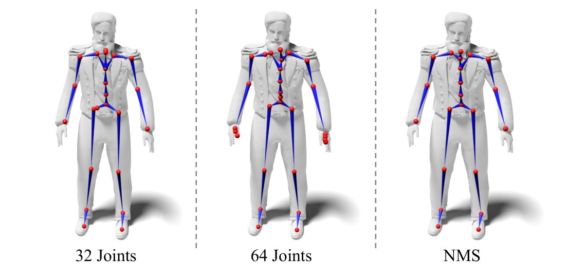
As mentioned in Sec. 4.2.1 of the main paper, the diffusion-based architectures support inference with an arbitrary number of predicted joints specified by a user. fig. S11 shows an example with two different number of joints, 32 and 64. Both predicted skeletons look reasonable based on the input mesh. An interesting observation is that with an increased number of joints from 32 to 64, the model tends to predict additional joints around the hands, while maintaining the sparsity at other locations, e.g.single joints at the knees. This offers an intuitive control over the granularity of the predicted rigs.

In addition, we also find an extra non-maximum suppression (NMS) step leads to cleaner results and hence better numbers on our benchmarks, as visualized on the last column in fig. S11. Therefore, for all the quantitative evaluations of the diffusion-based models, we use this extra NMS step. Specifically, we sample 128 points and retain only one joint with each $0.05^{3}$ voxel.

B.3. Additional Quantitative Results

Model	CD $\downarrow$	EMD $\downarrow$	Precision $\uparrow$	Recall $\uparrow$
Pinocchio (Baran and Popović, 2007)	0.198	0.659	52.7%	24.9%
RigNet^† (Xu et al., 2020)	0.144	0.173	54.6%	57.1%
trained on Anymate-small (14K)
RigNet (Xu et al., 2020)	0.139	0.166	49.4%	51.6%
Mich-Regress	0.099	0.124	71.6%	70.9%
Mich-Diff_Concat	0.142	0.175	42.2%	50.9%
Mich-Diff_Cross	0.128	0.160	65.1%	64.9%
Mich-Vol_Implicit	0.147	0.127	70.3%	73.7%
Mich-Vol_TriPlane	0.198	0.186	56.6%	49.2%
Bert-Regress	0.091	0.113	74.7%	79.8%
Bert-Diff_Concat	0.147	0.177	43.9%	58.3%
Bert-Diff_Cross	0.137	0.167	36.9%	30.5%
Bert-Vol_Implicit	0.123	0.126	73.2%	69.9%
Bert-Vol_TriPlane	0.192	0.171	63.8%	50.9%
trained on Anymate-train (225K)
RigNet (Xu et al., 2020)	0.089	0.127	53.4%	51.2%
Bert-Regress	0.077	0.098	80.2%	84.4%
Mich-Diff_Cross	0.085	0.107	76.9%	81.3%

Table S5. Quantitative Evaluation of Joint Prediction on Anymate-test corresponding to Tab. 2 of the main paper. ^†Model weights released by RigNet (Xu et al., 2020) trained on ModelsResource-RigNetv1 (Xu et al., 2019).

Model	CE $\downarrow$	Cos $\uparrow$	MAE $\downarrow$	Precision $\uparrow$	Recall $\uparrow$
GeoVoxel (Dionne and de Lasa, 2013)	3.569	0.407	0.056	27.8%	34.6%
RigNet^† (Xu et al., 2020)	1.672	0.661	0.029	37.2%	89.9%
trained on Anymate-small (14K)
RigNet (Xu et al., 2020)	1.573	0.671	0.031	37.2%	89.9%
Mich-Concat	1.169	0.754	0.029	59.4%	87.1%
Mich-Cross	1.270	0.766	0.026	67.9%	86.8%
Bert-Concat	1.242	0.768	0.027	61.2%	90.2%
Bert-Cross	1.134	0.801	0.025	68.8%	88.5%
trained on Anymate-train (225K)
RigNet (Xu et al., 2020)	1.521	0.693	0.028	37.2%	89.9%
Bert-Cross	0.741	0.915	0.015	82.4%	93.2%

Table S6. Quantitative Evaluation of Skinning Weight Prediction on Anymate-test corresponding to Tab. 4 of the main paper. ^†Model weights released by RigNet (Xu et al., 2020) trained on ModelsResource-RigNetv1 (Xu et al., 2019).

trained on Anymate-small (14K)
Model	CD $\downarrow$	EMD $\downarrow$	Precision $\uparrow$	Recall $\uparrow$
Pinocchio (Baran and Popović, 2007)	0.213	0.512	36.6%	25.1%
RigNet^† (Xu et al., 2020)	0.092	0.124	67.4%	75.7%
RigNet (Xu et al., 2020)	0.108	0.179	63.8%	48.5%
Mich-Regress	0.081	0.099	76.6%	73.5%
Mich-Diff_Concat	0.117	0.137	55.4%	61.2%
Mich-Diff_Cross	0.091	0.101	68.9%	69.7%
Mich-Vol_Implicit	0.113	0.121	65.3%	68.5%
Mich-Vol_TriPlane	0.155	0.167	49.2%	57.3%
Bert-Regress	0.075	0.091	74.4%	80.4%
Bert-Diff_Concat	0.134	0.154	48.2%	53.9%
Bert-Diff_Cross	0.117	0.137	53.4%	65.6%
Bert-Vol_Implicit	0.105	0.116	69.8%	71.7%
Bert-Vol_TriPlane	0.147	0.162	55.4%	59.0%
trained on Anymate-train (225K)
RigNet (Xu et al., 2020)	0.121	0.291	53.6%	43.7%
Bert-Regress	0.057	0.068	85.6%	88.9%
Mich-Diff_Cross	0.070	0.088	78.7%	83.0%

Table S7. Quantitative Evaluation of Joint Prediction on RigNet-test (Xu et al., 2020). ^†Model weights released by RigNet (Xu et al., 2020) trained on ModelsResource-RigNetv1 (Xu et al., 2019).

trained on Anymate-small (14K)
Model	Precision $\uparrow$	Recall $\uparrow$
RigNet^† (Xu et al., 2020)	76.5%	75.3%
RigNet (Xu et al., 2020)	73.2%	71.5%
Mich-Token	65.3%	63.5%
Mich-2Branch	73.7%	71.5 %
Bert-Token	69.9%	66.8 %
Bert-2Branch	74.6%	72.3%
trained on Anymate-train (225K)
RigNet (Xu et al., 2020)	68.8%	67.6%
Bert-2Branch	89.8%	88.7%

Table S8. Quantitative Evaluation of Connectivity Prediction on RigNet-test (Xu et al., 2020). ^†Model weights released by RigNet (Xu et al., 2020) trained on ModelsResource-RigNetv1 (Xu et al., 2019).

trained on Anymate-small (14K)
Model	CE $\downarrow$	Cos $\uparrow$	MAE $\downarrow$	Precision $\uparrow$	Recall $\uparrow$
GeoVoxel (Dionne and de Lasa, 2013)	3.012	0.451	0.071	26.4%	32.9%
RigNet^† (Xu et al., 2020)	1.054	0.742	0.056	34.9%	93.7%
RigNet (Xu et al., 2020)	1.122	0.723	0.059	34.7%	93.4%
Mich-Concat	0.758	0.794	0.034	61.6%	93.1%
Mich-Cross	0.783	0.810	0.031	68.2%	92.5%
Bert-Concat	0.727	0.821	0.032	63.9%	95.4%
Bert-Cross	0.711	0.829	0.029	67.9%	93.9%
trained on Anymate-train (225K)
RigNet (Xu et al., 2020)	1.012	0.744	0.052	34.8%	94.0%
Bert-Cross	0.534	0.891	0.023	73.2%	96.0%

Table S9. Quantitative Evaluation of Skinning Weight Prediction on RigNet-test (Xu et al., 2020). ^†Model weights released by RigNet (Xu et al., 2020) trained on ModelsResource-RigNetv1 (Xu et al., 2019).

Model	CD $\downarrow$	EMD $\downarrow$	Precision $\uparrow$	Recall $\uparrow$
RigNet^† (Xu et al., 2020)	0.092	0.124	67.4%	63.7%
Mich-Regress^∗	0.023	0.034	90.7%	82.1%
Mich-Diff_Cross^∗	0.032	0.041	81.7%	78.8%

Table S10. Quantitative Evaluation of Joint Prediction on RigNet-test (Xu et al., 2020). ^†Model weights released by RigNet (Xu et al., 2020) trained on ModelsResource-RigNetv1 (Xu et al., 2019). ^∗Model trained on ModelsResource RigNetv1 (Xu et al., 2019).

Model	ED $\downarrow$	Precision $\uparrow$	Recall $\uparrow$	CD-B2B $\downarrow$
RigNet^† (Xu et al., 2020)	2.52	84.5%	77.3%	0.012
Bert-2Branch^∗	0.81	96.7%	96.6%	0.002

Table S11. Quantitative Evaluation of Connectivity Prediction on RigNet-test (Xu et al., 2020). ^†Model weights released by RigNet (Xu et al., 2020) trained on ModelsResource-RigNetv1 (Xu et al., 2019). ^∗Model trained on ModelsResource RigNetv1 (Xu et al., 2019).

Model	IoU $\uparrow$	CD-J2B $\downarrow$	CD-B2B $\downarrow$
RigNet^† (Xu et al., 2020)	63.4%	0.051	0.050
Mich-Regress^∗ + Bert-2Branch^∗	85.6%	0.017	0.019
Mich-Diff_Cross^∗ + Bert-2Branch^∗	79.8%	0.021	0.023

Table S12. Quantitative Evaluation of Skeleton Prediction on RigNet-test (Xu et al., 2020). ^†Model weights released by RigNet (Xu et al., 2020) trained on ModelsResource-RigNetv1 (Xu et al., 2019). ^∗Model trained on ModelsResource RigNetv1 (Xu et al., 2019).

Model	CE $\downarrow$	Cos $\uparrow$	L1-avg $\downarrow$	Precision $\uparrow$	Recall $\uparrow$
RigNet^† (Xu et al., 2020)	1.054	0.742	0.57	60.9%	89.7%
Bert-Cross^∗	0.458	0.922	0.26	79.4%	96.4%

Table S13. Quantitative Evaluation of Skinning Weight Prediction on RigNet-test (Xu et al., 2020). ^†Model weights released by RigNet (Xu et al., 2020) trained on ModelsResource-RigNetv1 (Xu et al., 2019). ^∗Model trained on ModelsResource RigNetv1 (Xu et al., 2019).

We include four additional sets of evaluations. First, we additionally report the Precision and Recall metrics for both joint and skinning predictions, as explained in appendix D. Second, we also evaluate the performance of RigNet (Xu et al., 2020) using the pre-trained weights officially released by the authors, as an additional baseline, marked with ^† in all tables. What’s more, we evaluate all of the models on the same test set used by RigNet (Xu et al., 2020) (RigNet-test) containing 270 instances, and report the results in tables S7, S8 and S9. Lastly, for a more comprehensive comparison of the models’ efficiency, we conducted training of our proposed baselines on the RigNet-train dataset and evaluated their performance on the RigNet-test dataset. The results are reported in tables S10, S11, S12 and S13. We found that our model consistently outperforms RigNet significantly, even on the RigNet-train set. The key factor behind this enhancement is our elimination of certain assumptions present in RigNet, combined with our shift from GNN-based to transformer-based architectures for rigging prediction.

For joint prediction, from tables S5 and S7, it is evident that all our models trained on the Anymate-train exhibit superior performance, compared to the existing methods across all metrics. On RigNet-test, the RigNet model trained on our Anymate Dataset in fact performs worse compared to the originally released weights (pretrained on the RigNet dataset). This could be attributed to the fact that the training data used for the released weights model aligns closely with the domain of the RigNet-test.

For connectivity prediction, based on table S8, we can observe that the pre-trained RigNet has a competitive performance compared to our models trained on Anymate-small. However, when trained on Anymate-train, our models greatly surpass the performance of the pre-trained RigNet. This emphasizes the scalability of our framework.

For skinning weight prediction, based on tables S6 and S9, we can observe that RigNet demonstrates notably high recall but low precision, primarily because it predicts the skinning weight for only the five nearest bones. This limitation often leads to weights being assigned to all five nearest bones, which in turn affects precision negatively. Conversely, our model strikes a good balance between precision and recall, performing the best on both the Anymate-test and RigNet-test.

Appendix C Inference Time Analysis

We have reported the training time of different models in the tables in the main paper. During inference, RigNet takes over 10 minutes per instance to predict skeleton and skinning weights, while our final model only takes less than 3 seconds, significantly enhancing efficiency.

Appendix D Additional Technical Details

D.1. Joint Prediction

Metrics.

As mentioned in Sec. 4.2.3 in the main paper, we use two metrics for quantitative evaluation of the joint prediction accuracy: Chamfer Distance (CD) and Earth Mover’s Distance (EMD). The Chamfer Distance is computed as follows:

(S2)		$\displaystyle L_{\text{CD}}(\hat{\mathcal{J}},\mathcal{J})$	$\displaystyle=\frac{1}{K_{\text{pred}}}\sum_{\hat{\mathbf{J}}_{i}\in\hat{\mathcal{J}}}\min_{\mathbf{J}_{j}\in\mathcal{J}}\\|\hat{\mathbf{J}}_{i}-\mathbf{J}_{j}\\|_{2}^{2}$
(S2)			$\displaystyle+\frac{1}{K_{\text{gt}}}\sum_{\mathbf{J}_{j}\in\mathcal{J}}\min_{\hat{\mathbf{J}}_{i}\in\hat{\mathcal{J}}}\\|\mathbf{J}_{j}-\hat{\mathbf{J}}_{i}\\|_{2}^{2},$

where $\hat{\mathcal{J}}=\{\hat{\mathbf{J}}_{i}\}_{i=1}^{K_{\text{pred}}}$ and $\mathcal{J}=\{\mathbf{J}_{j}\}_{j=1}^{K_{\text{gt}}}$ are the two sets of predicted and (annotated) ground-truth (GT) 3D joint locations respectively.

The Earth Mover’s Distance is defined as solving the optimization problem of:

(S3)

L_{\text{EMD}}(\hat{\mathcal{J}},\mathcal{J})=\min_{f_{ij}}\frac{1}{K_{\text{pred}}}\sum_{i=1}^{K_{\text{pred}}}\sum_{j=1}^{K_{\text{gt}}}d_{ij}\cdot f_{ij},

where $d_{ij}=\|\hat{\mathbf{J}}_{i}-\mathbf{J}_{j}\|_{2}^{2}$ is the distance between two joints, $f_{ij}>0$ is the flow that satisfies following:

(S4)

\sum_{i=1}^{K_{\text{pred}}}{f_{ij}}=\frac{1}{K_{\text{gt}}},~~\sum_{j=1}^{{K_{\text{gt}}}}{f_{ij}}=\frac{1}{K_{\text{pred}}},~~\sum_{i=1}^{K_{\text{pred}}}\sum_{j=1}^{{K_{\text{gt}}}}{f_{ij}}=1.

In practice, we use the implementation in Point-Cloud-Utils (Williams, 2024) to calculate the EMD.

Both metrics evaluate the “closeness” between the two sets of points. In addition, we also evaluate the “correctness” of the predicted joints using the standard Precision metric, and the “coverage” using the Recall metric, after identifying the closest mapping between two point sets. Specifically, Precision is calculated as the ratio of correctly predicted joints (those with a distance to their nearest GT joint lower than the threshold) to the total number of predicted joints. Recall, on the other hand, is the ratio of correctly matched GT joints to the total number of GT joints. The threshold is set to 0.05 here.

D.2. Connectivity Prediction

Metrics.

Similarly, we use Precision and Recall to assess the connectivity prediction. Precision is computed as the proportion of correctly predicted pairs among all predicted pairs, whereas Recall is the proportion of correctly predicted pairs among all GT pairs.

D.3. Skinning Weight Prediction

Loss Function.

As described in Sec. 4.4, we train the skinning weight prediction models using the cosine similarity loss. Specifically, given the two predicted and ground-truth skinning weight matrices, $\hat{\mathbf{W}}$ and $\mathbf{W}$ , across $N$ vertex and $K_{\text{gt}}$ joints, the loss is computed as:

(S5)

L_{\text{cos}}(\hat{\mathbf{W}},\mathbf{W})=\frac{1}{N}\sum_{i=1}^{N}\left(1-\texttt{cos}(\mathbf{\hat{W}}_{i},\mathbf{W}_{i})\right),

where cos denotes the cosine similarity between the two vectors $\mathbf{\hat{W}}_{i}$ and $\mathbf{W}_{i}$ .

Metrics.

We report three evaluation metrics for the skinning weight prediction: Cross Entropy (CE), Cosine Similarity (Cos), and Mean Absolute Error (MAE).

MAE is computed as the average difference between each vertex and each bone:

(S6)

L_{\text{MAE}}(\hat{\mathbf{W}},\mathbf{W})=\frac{1}{N{K_{\text{gt}}}}\sum_{i=1}^{N}\sum_{j=1}^{K_{\text{gt}}}|\hat{w}_{ij}-w_{ij}|,

where $\hat{w}_{ij}$ and $w_{ij}$ are the elements of the predicted and GT skinning weight matrices, $\hat{\mathbf{W}}$ and $\mathbf{W}$ , respectively.

CE is computed as the average cross-entropy over all vertices with the ground truth:

(S7)

L_{\text{CE}}(\hat{\mathbf{W}},\mathbf{W})=\frac{1}{N{K_{\text{gt}}}}\sum_{i=1}^{N}\sum^{K_{\text{gt}}}_{j=1}\left(-w_{ij}\log{{\hat{w}_{ij}}}\right).

In addition, we also report the Precision and Recall in tables S6 and S9. For skinning prediction, Precision is determined by identifying the set of bones that significantly “influence” each vertex, with a skinning weight exceeding a threshold of 0.05. It is calculated as the proportion of the “influential” bones identified based on the predicted skinning that align with those identified based on the ground-truth skinning weights.

Recall, conversely, is computed as the ratio of “influential” bones identified based on the ground-truth skinning weights that successfully match those derived from the predicted skinning weights.

Appendix E Rest Pose Derivation

As mentioned in Sec. 3.1 of the main paper, the rest pose transformation $G_{b}(\xi^{*})$ can be derived from the head and tail joint locations of the bones, $\{(\mathbf{J}_{b}^{\text{head}},\mathbf{J}_{b}^{\text{tail}})\}_{b=1}^{B}$ , in a kinematic tree structure.

Specifically, $G_{b}(\xi^{*})$ (in the world coordinate frame) is a composition of the transformation $g_{b}$ of the bone $b$ itself (in its local coordinate frame) and the composed transformation $G_{\pi(b)}$ of its parent, bone $\pi(b)$ , following the kinematic tree:

(S8)

G_{b}=G_{\pi(b)}\circ g_{b},

where $G_{1}=g_{1}$ and $g_{b}(\xi_{b}^{*})\in SE(3)$ is a $4\times 4$ transformation matrix, with a rotation matrix $\mathbf{R}_{\xi_{b}^{*}}\in\mathbb{R}^{3\times 3}$ and a translation vector $\mathbf{t}_{\xi_{b}^{*}}\in\mathbb{R}^{3\times 1}$ :

(S9)

g_{b}(\xi_{b}^{*})=\begin{bmatrix}\mathbf{R}_{\xi_{b}^{*}}&\mathbf{t}_{\xi_{b}^{*}}\\ 0&1\\ \end{bmatrix}.

Note that the local coordinate frame of each bone $b$ can be defined arbitrarily with $\mathbf{R}_{\xi_{b}^{*}}$ and $\mathbf{t}_{\xi_{b}^{*}}$ . In particular, we choose an intuitive definition, where each bone is a unit vector originating from the origin pointing towards $(0,0,1)$ on the $z$ -axis of its local coordinate frame, and the $x$ -axis is always horizontal (w.r.t.the world coordinate frame). As such, the rest-pose rotation matrix $\mathbf{R}_{\xi_{b}^{*}}$ and translation vector $\mathbf{t}_{\xi_{b}^{*}}=(0,0,|\mathbf{J}_{b}^{\text{tail}}-\mathbf{J}_{b}^{\text{head}}|)$ can be obtained via a similar procedure as the camera lookat matrix (from head joint $\mathbf{J}_{b}^{\text{head}}$ to tail joint $\mathbf{J}_{b}^{\text{tail}}$ ).

Training Hyper-Parameter	Value
Epoch	200
Batch Size	16
Learning Rate	1e-4
Learning Rate Decay	2e-5 at epoch 100
Optimizer	Adam

Model	Layer Number & Type	Layer Dimensions
Encoder-Mich	25 TFLayer	768
Encoder-Bert	12 TFLayer	384
Joint-Regress	1 TFLayer	768
Joint-Diff_Concat	4 TFLayer	512
Joint-Diff_Cross	4 DenoiseBlock	768
Joint-Vol_Implicit	1 TFLayer	768
Joint-Vol_TriPlane	7 CNNBlock	512
Conn-Token	4 TFLayer	768
Conn-2Branch	5 TFLayer	768
Skin-Concat	4 TFLayer	768
Skin-Cross	4 TFLayer	768

Table S14. Implementation Details: Hyper-Parameter and Model Size. In the model details table, "TF" denotes "Transformer", and "Layer Dimensions" represents the size of the token used by Transformer or the majority channel size used by CNNBlock.

Appendix F Implementation Details

Details of the architecture designs for each module and hyper-parameter setting are listed in table S14.

Appendix G Limitation and Failure Cases Analysis

While our framework has proven efficient and robust on a wide range of examples, we do observe some limitations that require further exploration in future work. Firstly, despite training on a vast dataset, our model occasionally makes incorrect skeleton predictions under certain circumstances. There are two common failure cases: (1) when some parts of the mesh penetrate or are too close to other parts, it may cause failure in skinning prediction, as illustrated in fig. S13; (2) when the mesh contains some bulky parts, it may predict too many joints within those regions, resulting in issues in the subsequent modules, as depicted in fig. S13. (1) could be addressed by incorporating geometric regularizations and/or pre-processing the input mesh, whereas (2) could potentially be mitigated with an adjustable granularity control. In addition, skeleton-based rigging systems face inherent limitations in modeling certain complex deformations, such as simulating elastic materials or capturing nuanced facial expressions. These challenges may be better addressed through alternative rigging representations like neural cages or other physics-informed approaches. We leave the exploration of these specialized deformation problems to future work.