Bridging Econometrics and AI: VaR Estimation via Reinforcement Learning and GARCH Models
Abstract
In an environment of increasingly volatile financial markets, the accurate estimation of risk remains a major challenge. Traditional econometric models, such as GARCH and its variants, are based on assumptions that are often too rigid to adapt to the complexity of the current market dynamics. To overcome these limitations, we propose a hybrid framework for Value-at-Risk (VaR) estimation, combining GARCH volatility models with deep reinforcement learning. Our approach incorporates directional market forecasting using the Double Deep Q-Network (DDQN) model, treating the task as an imbalanced classification problem. This architecture enables the dynamic adjustment of risk-level forecasts according to market conditions. Empirical validation on daily Eurostoxx 50 data covering periods of crisis and high volatility shows a significant improvement in the accuracy of VaR estimates, as well as a reduction in the number of breaches and also in capital requirements, while respecting regulatory risk thresholds. The ability of the model to adjust risk levels in real time reinforces its relevance to modern and proactive risk management.
Keywords: Deep reinforcement learning, Directional prediction, Imbalanced class problem, Value-at-Risk
1 Introduction
Forecasting stock prices using empirical data is a central topic in financial research. In recent years, the growth of technology and the massive availability of data have heightened interest in the use of machine learning models in the analysis of financial markets. These models help to capture the inherent complexity of financial data, characterized by its nonlinearity, hidden structures, and dynamic evolution in response to various factors. However, in the context of risk management and portfolio optimization, the analysis of stock market returns is more relevant than the study of asset prices. Returns are often stationary, which makes for a more robust analysis, and, in accordance with the central limit theorem, they can sometimes be approximated by a normal distribution. However, this assumption is questionable given the stylized facts of financial time series: non-linear autocorrelation, asymmetric distribution tails, volatility clustering, and leverage. These features make the prediction of returns more complex than that of prices, as illustrated in figure 1, where we observe that conventional models struggle to predict excess returns, whether positive or negative.


This difficulty in capturing strong positive and negative variations is also observed in machine learning and deep learning models, despite their great flexibility and ability to model complex non-linear relationships.
These models are based on optimization algorithms that require large volumes of data to efficiently learn the underlying dynamics of financial markets, particularly when dealing with rare and extreme events (Pokou, 2022).
Extreme events, by definition, are infrequent in financial time series, which limits the capacity of these models to extract exploitable regularities (Fawcett and Provost, 1997).
The most machine learning and deep learning models are trained by minimizing mean square error (MSE) or similar loss functions, which give disproportionate weight to errors on the most common values at the expense of extreme events.
These approaches lead to a bias in favor of predictions close to the mean of historical data, reducing the sensitivity of the model to strong market variations (Goodfellow et al., 2016).
As a result, even advanced architectures such as recurrent neural networks (RNN), temporal convolutional neural networks (TCN) or hybrid model combinations (e.g. ARIMA-ANN) fail to accurately anticipate these rare events (Zhang, 2003; Tealab, 2018; Pokou et al., 2024b).
This difficulty is partly related to the efficient market hypothesis Fama (1970), which postulates that prices incorporate all available information, making their prediction uncertain.
Faced with the difficulty of accurately predicting the returns of the stock market, several authors (Kanas, 2001; Nyberg, 2011; Oh and Sheng, 2011; Alostad and Davulcu, 2017; Becker and Leschinski, 2018; Chandrasekara et al., 2019) have proposed reformulating this problem into a classification task, focusing no longer on the exact value of the returns, but on their sign (positive or negative). This approach, known as directional return prediction, is based on the idea that the key to many investment strategies is not to anticipate the precise return but rather to determine the future direction of the market. For this purpose, a threshold is defined to classify returns into distinct categories: generally, this threshold is set at zero, thus distinguishing positive from negative returns. However, some studies (Chung and Hong, 2007; Linton and Whang, 2007) have proposed more sophisticated thresholds, based, for example, on multiples of the standard deviation or quantiles of the return distribution, to better capture significant market movements.
In this study, we extend this approach by adopting a threshold, inspired by the work of Nevasalmi (2020). Rather than simply distinguishing between positive and negative returns, we introduce a finer classification that isolates some of the noise and better identifies extreme returns, whether strongly positive or negative. This approach refines the prediction by focusing on the most significant market movements. However, it leads to class imbalance, making the classification task more complex. To the best of our knowledge, this problem has been little explored in the context of financial time series.
However, financial risk management relies on measures such as Value-at-Risk (VaR), which estimates the maximum potential loss of a portfolio over a given time horizon with a certain level of confidence. Originally developed in the work of Markowitz (1952, 1959), VaR has been widely adopted in banking regulation (Basel I, II, III). But despite its importance, VaR has certain limitations:
-
•
Overestimation of risk, leading to a waste of capital
-
•
Underestimation of risk, increasing exposure to excessive losses.
These limitations have led to the development of alternative measures, such as Expected Shortfall (ES), which is more mathematically robust but whose backtesting methods remain less well established. In this study, we focus on improving VaR prediction by incorporating directional prediction of returns into its estimation. Traditionally, directional return forecasting relies on statistical and supervised machine learning models, such as logistic regression (LR), gradient boosting (GBM), random forests (RF), neural networks (MLP, LSTM, etc.). (Tang et al., 2008). However, these approaches suffer when there is a class imbalance, which is precisely the case in our study. To mitigate this effect, various rebalancing techniques have been developed:
-
•
Resampling methods: oversampling (SMOTE, ADASYN) or undersampling (ENN, Tomek-Links)
-
•
Ensemble methods: boosting, bagging and random forests
-
•
Cost-sensitive learning, which penalizes errors on the minority class.
However, these approaches can induce bias or overfitting. Deep reinforcement learning (DRL) represents a promising alternative, as it directly learns an optimal policy for managing class imbalance. Successfully applied in various fields (Mnih et al., 2013; Gu et al., 2017; Mao et al., 2016; Zhao et al., 2017; Yu et al., 2021), DRL has recently been used in finance (Deng et al., 2016; Liu et al., 2020; Yang et al., 2020; Zhang et al., 2020; Pokou et al., 2024a). Its integration into our approach improves the robustness of directional forecasting and, by extension, VaR estimation.
The use of Deep Reinforcement Learning (DRL) to estimate risk measures such as Value-at-Risk (VaR) and Expected Shortfall (ES) has recently attracted growing interest in quantitative finance. Morimura et al. (2012) proposed a parametric approach to estimate the density of returns via an extension of the Bellman equation, leading to robust and risk-sensitive TD learning algorithms.
In a similar framework, Ying et al. (2022) developed the CVaR-Proximal-Policy-Optimization (CPPO) algorithm, constraining policy optimization to a bound on Conditional Value-at-Risk (CVaR), thus guaranteeing more robust learning in the face of uncertainties.
Furthermore, Barrera et al. (2022) have studied nonparametric learning of VaR and ES using generalization bounds derived from Vapnik-Chervonenkis statistical theory, highlighting approximation methods based on quantile regressions and neural networks. From a complementary perspective, Clements et al. (2019) have examined epistemic and random uncertainties in DRL applied to Q values, proposing a DQN algorithm adjusted for these uncertainties and demonstrating improved stability of risk estimates. In addition, recent work on robust estimation of ES in heavy-tailed distributions has highlighted the limitations of traditional approaches and the potential contribution of DRL to capture the extreme dynamics of financial returns. These contributions illustrate the advances of DRL in financial risk modeling while raising challenges regarding the interpretability of learned policies and the stability of risk estimates in uncertain environments.
In contrast to this work, our approach applies DRL to directional forecasting of stock returns in order to improve VaR estimation. By reformulating the problem as a directional classification task rather than a classical return regression, we take advantage of DRL to better manage the class imbalance and refine the forecast accuracy. This approach aims to overcome the limitations of traditional methods by providing a more reliable estimate of risk, thus minimizing the overestimation and underestimation errors common in VaR calculations.
The main contribution of this paper lies in the development of a new empirical approach to Value-at-Risk (VaR) estimation. In contrast to traditional approaches, our method takes advantage of directional prediction of returns to dynamically adjust the VaR, enabling better adaptation to market fluctuations. In addition, it incorporates efficient class imbalance management thanks to the capabilities of Deep Reinforcement Learning (DRL), which considerably improves the stability and relevance of risk forecasts. Finally, this approach stands out for its ability to increase the accuracy and robustness of VaR, simultaneously reducing the number of violations and excessive capital allocation, thus offering a more effective framework for financial risk management.
The paper is structured to guide the reader progressively through our methodological approach and its empirical implications. First, Section 2 introduces the methodological framework, detailing the theoretical foundations and models used for adaptive Value-at-Risk estimation. The next sections 3 and 4 present the empirical results obtained, together with an in-depth analysis of their robustness, highlighting the performance of our approach compared to conventional methods. Finally, Section 5 concludes the study by summarizing the main contributions and opening the discussion on prospects for improvement and future application of our model.
2 Methodology
Let be the closing price of an asset at time , so the logarithmic return at time over a unit time interval is defined as .
2.1 Value-at-Risk
The Value-at-Risk (VaR) is the quantile of the return distribution and represents the loss that will be exceeded in a proportion of cases during the next period. Then we have :
| (1) |
where is a probability generally set at or . After a short demonstration in a few steps, we have the following :
| (2) |
where represents the inverse return distribution function, also known as the quantile function.
VaR has gained popularity due to the simplicity of implementation and the ability to make no assumptions about the parametric form of return distributions.
Although we may be tempted by non-parametric solutions, it is important to remember that parametric VaR is very useful.
In particular, a model capable of taking into account stylized facts about asset return distribution was defined. The normal distribution is often used, except that unconditional return distributions usually have much fatter tails. Using first two conditional moments of the distribution, it is possible to present returns time series in this form:
| (3) |
where is the return at time , is the conditional mean, is the conditional volatility of the return and is the residual of the process (innovation term).
It is assumed that are distributed independently and identically and follow a known theoretical distribution with zero mean and unit variance. If the random variable is normally distributed, we have :
| (4) |
where is the cumulative distribution function of a standard normal variable.
Given these stylized facts, and in particular the nonnormality of asset return distributions, a standardized Student distribution would be the most plausible (with zero mean and unit variance) with degrees of freedom, giving :
| (5) |
where denotes the distribution function of Student’s standard distribution.
This expression will be useful for independently modeling the dynamics of and .
In our case, will be modeled as arithmetic mean returns, which take values very close to zero.
Conditional volatility will be modeled directly using the GARCH (resp. GJR-GARCH) time series.
2.2 GARCH models
Introduced by Bollerslev (1986), the GARCH(p,q) model can be defined by assuming that is a stochastic process decomposable in terms of expected returns and residuals, as follows:
where
| (6) |
with , , , , and independent, identically distributed variable .
The GARCH (1,1) model is the simplest and most commonly used univariate model and can be defined as follows
| (7) |
where the variance process in GARCH(1,1) is stationary when .
The convergence rate depends on .
As persistence is closer to 1, it takes longer for a shock to be forgotten by the market.
Glosten, Jagannathan, and Runkle (1993) proposed the GJR-GARCH(p,q) model to overcome GARCH’s inability to differentiate between negative and positive shocks and to take leverage into account. It can be defined as follows:
| (8) |
In particular, GJR-GARCH(1,1) is expressed as follows:
| (9) |
where positivity of conditional variances is ensured by , , and , therefore, if , bad news has a greater impact on conditional variance than good news, and in addition, stationarity of variances is possible provided that .
2.3 Threshold selection for directional prediction
Although regression models were the most intuitive approach to predicting future values of stock market asset returns, the current trend shows that classification models appear to have better predictive power. Except that this requires transforming a prediction problem into a classification problem. Classes are determined according to the desired goal via a threshold. In trading, for example, it is possible to construct strategies based on return signs (positive or negative) or excess returns, i.e. the difference between returns and the risk-free rate (). In directional prediction, binary dependent variables are created from return series using an indicator function
where is a given threshold (often ).
In our study, given that the objective is to improve value-at-risk performance, the chosen threshold is the lowest VaR violation.
| (10) |
is the number of VaR violations.


2.4 Proposed VaR model
Let be the value-at-risk with a threshold calculated using a GARCH or GJR-GARCH model. Let us consider a classification model that assigns at each time t+1 a predicted risk category among two possible states:
-
•
"Low risk": low level of risk
-
•
"High risk": high level of risk
Definition 1 (Classification-Adjusted Value at Risk).
The Classification-Adjusted Value at Risk, noted is defined as follows:
| (11) |
where :
-
•
are calibration parameters determining the extent of the reduction or increase in .
-
•
is the prediction of the future risk level made by the machine learning models we will present in the next section.

The proposed VaR model has properties identical to those of the original VaR. Knowing that it is not possible for to have two risk levels at the same time, one of equation (11)’s components becomes null, and with VaR’s positive homogeneity property, the proof is obvious.
2.5 Machine Learning
In figure 3, we can see that we are dealing with an unbalanced class problem.
This is a major challenge in training traditional Machine Learning models, including logistic regression (Dreiseitl and Ohno-Machado, 2002), Support Vector Machine (SVM) (Vapnik, 1999; Tang et al., 2008) and various neural network architectures such as perceptron (ANN), multilayer perceptron (MLP) (Rosenblatt, 1958; Murtagh, 1991), recurrent neural networks (RNN) (Ampomah et al., 2020; Sunny et al., 2020) and Temporal Convolutional Network (TCN) (Lea et al., 2016).
In such scenarios, models tend to favor the majority class, leading to a strong imbalance in predictions, where minority cases are often ignored.
Although sampling techniques such as under-sampling (ENN111Edited Nearest Neighbors, Random Undersampling, Tomek Links) (Kotsiantis et al., 2006; Barandela et al., 2004; Elhassan and Aljurf, 2016; Zeng et al., 2016; Pereira et al., 2020) and over-sampling (ADASYN222Adaptive Synthetic Sampling, SMOTE333Synthetic Minority Over-sampling Technique, Random Oversampling) (Chawla et al., 2002; Han et al., 2005; Zhang and Li, 2014) have been developed to alleviate this problem, they themselves present certain limitations.
Undersampling reduces the size of the majority class, which can lead to a loss of valuable information and impair overall model performance.
In contrast, oversampling artificially increases the size of the minority class, but at the cost of an increased risk of overfitting, as synthetic observations may not faithfully reflect the actual distribution of the data.
Another key challenge in these contexts lies in error measurement and model optimization. Standard cost functions such as cross-entropy loss or mean square error (MSE) are often inadequate for unbalanced classes, as they are dominated by the majority class.
This results in weight updates that minimize overall loss, but without improving the model’s ability to detect the minority class. Even by adjusting the weights of the loss function or modifying the evaluation metrics (such as using F1-score or recall instead of simple accuracy), classical supervised models struggle to learn effective representations in such an environment. Given these limitations, the Double Deep Q-Network (DDQN) appears to be a promising alternative. Unlike purely supervised models, DDQN is based on reinforcement learning, where the agent learns to optimize its decisions by interacting with a dynamic environment.
This approach enables more efficient exploration of classification strategies and better adaptation to imbalances, without depending directly on a pre-established class distribution. By maximizing a reward function, DDQN learns to handle rare classes in a more robust and adaptive way, offering a better alternative to classical supervised learning methods.
2.6 Reinforcement learning
Supervised learning, to which the above-mentioned models belong, relies on the use of labeled data to establish a relationship between inputs (features) and outputs (labels).
The aim is to learn a function that, after training, can generalize to new data and correctly predict the corresponding class. This type of learning is effective when the data are well balanced and when the relationship between the explanatory variables and the target variable is sufficiently clear.
However, it has significant limitations when applied to complex and dynamic problems, such as those involving high-class imbalance or requiring sequential decision-making.
In contrast, reinforcement learning proposes a fundamentally different paradigm. Rather than optimizing a cost function by minimizing the error between predictions and actual labels, the goal is to learn an optimal policy that maximizes the cumulative reward obtained by an agent interacting with an environment.
This process is based on a trial-and-error loop, where the agent explores different actions, observes their consequences, and gradually adjusts its strategy according to the rewards received.
This approach enables models to learn adaptively and autonomously, which is particularly useful for problems where the underlying rules are dynamic or partially unknown.
Introduced by Sutton and Barto (1998), reinforcement learning was designed to overcome the limitations of dynamic programming approaches (Puterman, 2014) and Monte Carlo methods (Gilks et al., 1995). Unlike dynamic programming, which requires explicit knowledge of the environment model and quickly becomes inapplicable in large state spaces, and Monte Carlo methods, which cannot easily exploit the temporal structure of decisions, reinforcement learning allows for a more flexible and scalable approach to the sequential decision problem.

The agent-environment interaction model is illustrated in figure 4. This problem is based on the Markov Decision Process (MDP) (White III and White, 1989), which formalizes the interaction between an agent and its environment in terms of states, actions, rewards, and probabilistic transitions. One of the key concepts of this approach is the value function, which estimates the expected future reward for a given action in a specific state. The optimization of this function is based on the Bellman equation, which describes the recursive relationship between state values and future rewards, and forms the basis of many modern reinforcement learning methods, including deep neural network approaches such as the Double Deep Q-Network (DDQN). Thus, by exploiting the principles of reinforcement learning and MDP, models based on autonomous agents can learn to make optimal decisions in complex and uncertain environments, where classical supervised approaches encounter significant limitations. This ability to adapt and learn progressively makes reinforcement learning a particularly relevant alternative in contexts where data are unbalanced, interaction rules evolve, and decision making needs to be optimized over the long term.
2.6.1 Markov Decision Process
A Markov decision process is a 5-tuple where :
-
is a finite set of states that the environment can reach such that they satisfy Markov’s property.
-
is a finite set of actions (action space). For our classification problem, where 0 represents the majority class (low risk) and 1 represents minority class (high risk). The action taken by an agent consists of predicting a class label.
-
is a state transition function.
We have : .
For a MDP, next state and reward depend solely on the current state and action. The probability of going from state to state at time by performing action is : -
gives a signal on actions quality performed by the agent during its learning phase. The reward function can be defined as the expected value of the reward of the action ’ when moving from one state to the next .
The agent is rewarded positively if it correctly classifies a sample (true positive and true negative), otherwise it is rewarded negatively (false positive and false negative). The reward can be defined as :
where more precisely equals the ratio of minority class cardinal to majority class cardinal.
-
1.
True Negative (TN):
The model predicts "Low risk" and the observation is actually "Low risk". In this case, the prediction is correct. The reward function awards to encourage the agent to correctly classify the majority class, without penalizing it too much. -
2.
False Negative (FN):
The model predicts "Low risk", but the observation is actually "High risk". This is a critical error, as a high-risk individual has been classified as "Low risk". This error is often more serious than the others The reward function assigns a penalty of , which is consistent with the weighting of the classes, since the minority class is less frequent and deserves more attention. -
3.
True Positive (TP):
The model predicts "High risk" and the observation is actually "High risk". This is a good prediction and should be encouraged. The associated reward is , which correctly rewards the detection of critical cases. -
4.
False Positive (FP):
The model predicts "High risk", but the observation is actually "Low risk". This is an error where a "Low risk" individual is classified as "High risk". Although this error is less serious than a FN, it has a cost in terms of unnecessary processing of a false alarm signal. The reward function assigns a penalty of to limit false positives.
-
1.
-
()is a discount factor used to balance immediate and future reward.
2.6.2 Policy
A policy defines the agent’s behavior at time where denotes the action performed by the agent in state :
| (12) |
The policy can be considered as a classifier and the agent must be able to learn to perform actions to maximize the expected total discounted return , according to the following equation.
| (13) |
where is the discount rate.
The optimal policy to obtain the expected maximum return from all states
| (14) |
2.6.3 State-Value function
The state value function is the expected return on a given state , which then follows a policy (Szepesvári (2010)), that is,
| (15) |
Thus, the optimal state value function is obtained under the optimal policy as:
| (16) |
2.6.4 Action-value function
The Q function, or the action value of the function, is the expected return from the state , by taking action , then by following policy , i.e.,
| (17) |
The optimal Q-function is the maximum of all policies:
| (18) |
According to Bellman’s expectation equation (Dixit (1990)), the Q function can be expressed as follows :
| (19) |
The optimal policy is found by maximizing the optimal state value function presented in equation (18). In other words, the best policy can be found by greedily choosing action in each state, which can be defined as :
| (20) |
Using Bellman’s optimality equation, we get :
| (21) |
2.6.5 Q-Learning
Since finding an optimal policy meant maximizing the Q function, Sutton (1988) proposed the temporal difference (TD) learning algorithm, which belongs to the class of tabular algorithms.
It is based on a bootstrapping operation that uses estimated values of future states to update the estimate of current state.
Then it saves the sample in a Q-table, from which the new estimate is obtained from a sample of possible options for the next state.
However, it becomes impossible to perform this backup due to enormous table size when environment has a large number of states or a continuous state space.
In this sense, Watkins (1989) introduced one of the most popular algorithms, Q-learning, which is an extension of the temporal difference to overcome this limitation.
So, instead of directly estimating a state value, we estimate each state-action pair value.
The goal is to gradually learn to associate states with actions in order to maximize expected rewards. These expected rewards (Q-values) are stored in a lookup table (Q-table), which functions as a memory that is updated as the agent explores its environment. The update rule is as follows:
| (22) |
where
-
is the Q-value for state and action .
-
is the learning rate that controls the size of the update.
-
is the reward obtained after taking action in state .
-
is the discount factor.
-
is the best Q-value for the next state.
2.6.6 Deep Q-Network
In Q-learning, the agent must maintain and update a set of Q-values for all pairs of states and actions.
However, in some applications, billions of unique possible states and several available actions are required.
As a result, the time and cost of calculating and updating all Q-values become virtually unfeasible, which is known as "the curse of dimensionality".
Deep Q Network (DQN) solves this problem by using a deep neural network to approximate the Q-function.
We then have where is a vector containing all weights and biases of the neural network. This neural network takes as input the current state and the action and estimates the Q-value. Furthermore, as mentioned earlier, DQN introduces Experience Replay and target network , two important enhancements that stabilize learning. -network used to estimate the target value is then :
| (23) |
where are the weights of the target network.
After randomly sampling mini-batches of experiments from the replay buffer, these experiments are used to train the Q-network to minimize the difference between predicted and target Q-values.
The weights of the neural network () are updated by the gradient descent of the loss function, which is represented by the following formula.
| (24) |
where are the weights of the current network.
To avoid instability during learning, Q-network () is updated at each learning step, whereas the target network () is updated less regularly by copying weights from Q-network.
2.6.7 Double Deep Q-Network
During Q-value estimation for each possible action in a given state with Deep Q-Network (DQN), a frequent problem is overestimation can lead to suboptimal policy selection. This is because the DQN uses the same network to guide exploration (maximum action selection) and to evaluate this action. Van Hasselt et al. (2016) proposed double deep Q-network (DDQN). An algorithm that advocates using two separate networks to estimate and evaluate actions, thus reducing over-estimation and improving learning stability. Instead of using update function expressed by equation (22), DDQN strategy is based on update functions presented in Jang et al. (2019)’s paper :
| (25) | ||||
| (26) |
Q-function () changes its value according to the value of the other Q-function (), and both functions determine the action. Dans ce cas, la valeur cible du DQN peut alors être écrite comme suit :
| (27) |
Consequently, the Q-network selects the action that results in the maximum Q-value for the next state, and the target network calculates the estimate of the Q-value based on the action selected previously. As with DQN, the use of the replay buffer makes learning more stable and efficient. During the learning process, experience replay is used to update the main network parameters, minimizing a differentiable loss function which, in the DDQN case, has the following form:
| (28) |
It also updates the second network weights , which are replaced by the target network weights . The weights of both networks are updated at different times, rather than simultaneously. At each learning stage, the valuation network is used to select the optimal action, but the target network is used to evaluate this action. Periodically, weights from the evaluation network are copied to the target network.
3 Empirical results
In this paper, we evaluate the performance of the proposed Value-at-Risk (VaR) model on the Euro Stoxx 50 index, a benchmark index of the 50 largest market capitalizations in the Eurozone. The data used come from Yahoo444https://fr.finance.yahoo.com/ Finance datastream, covering the period from September 1, 2008 to March 13, 2025.
The levels of risk of high risk and low risk will be defined according to the methodology presented in Section 2.3 and shown in figure 2(b).
An intuitive approach to predicting future risk levels would be to use the lagged returns of the individual components of the Euro Stoxx 50.
However, this methodology has several major limitations. Since its inception, the Euro Stoxx 50 has undergone several periodic revisions, with companies added or removed to reflect developments in European financial markets. This dynamic leads to discontinuity in the data series, which would complicate the training of machine learning models. This is because models based on these components would require constant updates whenever the index changed, making the analysis less robust and difficult to generalize. To overcome these limitations and ensure a more robust, generalizable, and stable approach over time, we opted for a more relevant selection of explanatory variables. As a first step, the stock market indices of the main economies in the euro zone would allow us to capture the overall economic development of European countries and identify general market trends.

Then, the currencies influencing European financial markets, which play a key role in the competitiveness of exporting companies and the attractiveness of foreign investment in Europe. We consider strategic currency pairs such as EUR/USD and EUR/GBP . In addition to macroeconomic variables, certain technical indicators are integrated to detect trends and signals of market reversal. To ensure a reliable and rigorous evaluation of the model, we divided the data chronologically into three distinct samples, as shown in figure 5. The training sample, which will make up the bulk of the data, is used to train the model by learning the relationships between the explanatory variables and the target variable. The validation set will be used to adjust the model’s hyperparameters and prevent overfitting, thus guaranteeing a better generalization. Then there is the test sample, which will be used only after training and validation, to assess the model’s actual performance on new observations and measure its ability to make reliable predictions in an unknown environment.

The variables were selected using the Boruta algorithm, a robust method specially designed for machine learning models. This algorithm determines the most relevant variables for predicting the risk level of financial asset returns, by identifying variables with a significant influence.
The Boruta algorithm (Kursa and Rudnicki, 2010; Kursa et al., 2010) is particularly well suited to complex datasets, such as those encountered in the financial field, where relationships between variables are often nonlinear and difficult to model. Analysis of the importance of variables using the Boruta algorithm (see figure 6) reveals a clear hierarchy of risk factors.
It is interesting to note that the past return of the Eurostoxx 50 at time (∧STOXX50E ret) only explains around 20% of the prediction, which may seem relatively modest given its direct link with the level of risk.
This limited contribution can be interpreted by the fact that market dynamics rapidly integrate past information, making simple returns less informative in non-linear models where memory effects, conditional volatility and structural interdependence predominate.
For comparison, FEZ, an ETF that faithfully replicates the Eurostoxx 50, provides additional information (17%) that could capture intraday price adjustments, liquidity effects, or market expectations not contained in the raw index.
CAC 40 (∧FCHI), representing a major component of Eurostoxx 50, provides an explanation of the order of 13%, reinforcing the idea that sector diversification within the index plays a differentiated role in risk formation.
And, volatility forecasts using the GARCH and GJR-GARCH models (varying significantly between 8 and 10%) confirm that the dynamics of expected volatility are a robust but not exclusive determinant of future risk, suggesting that market-perceived risk incorporates both feedback, structural, and behavioral expectation factors.
The low explanatory power of currencies such as EUR/USD (EURUSD=X) or EUR/GBP (EURGBP=X) in predicting risk levels can be explained by their global macroeconomic role, often uncorrelated with the specific dynamics of European equity markets.
These currency pairs mainly reflect broad monetary and geopolitical movements whose impact on the risk of the stock index is indirect or delayed.
Similarly, technical trading indicators such as buy/sell signals or ARIMA outputs are often built on local heuristics, and only partially capture structural risk components such as implied volatility, inter-market correlation, or sector sensitivity. Their simplifying and short-termist nature therefore limits their ability to explain complex risk phenomena. Table B1 shows the variables selected based on this algorithm.
| Assets | Mean (%) | Std (%) | Skewness | Kurtosis | Min | Max | ADF | Jarque-Bera |
| EURUSD=X | -0.007 | 0.724 | 0.782 | 113.692 | -0.143 | 0.160 | -12.606 | 2136941.801 |
| EURGBP=X | 0.001 | 0.598 | 0.166 | 62.569 | -0.111 | 0.110 | -33.930 | 647122.057 |
| BZ=F | -0.006 | 2.440 | -0.606 | 13.962 | -0.280 | 0.212 | -63.680 | 32465.986 |
| FEZ | 0.019 | 1.741 | -0.409 | 9.130 | -0.133 | 0.162 | -11.813 | 13887.933 |
| ∧FCHI | 0.017 | 1.409 | -0.188 | 8.671 | -0.131 | 0.106 | -21.735 | 12451.577 |
| ∧GDAXI | 0.034 | 1.399 | -0.087 | 8.742 | -0.131 | 0.116 | -20.348 | 12637.285 |
| ∧AEX | 0.022 | 1.311 | -0.327 | 9.672 | -0.114 | 0.100 | -12.401 | 15532.029 |
| ∧STOXX50E | 0.014 | 1.429 | -0.245 | 7.909 | -0.132 | 0.104 | -21.293 | 10379.093 |
| Features | Mean | Std | Min | Max |
| ∧STOXX50E Close | 3346.722 | 706.846 | 1809.980 | 5540.690 |
| ∧STOXX50E High | 3370.447 | 705.616 | 1823.250 | 5568.190 |
| ∧STOXX50E Low | 3321.543 | 707.570 | 1765.490 | 5506.570 |
| ∧STOXX50E Open | 3346.747 | 706.032 | 1812.780 | 5531.530 |
| BB upper | 3469.825 | 694.591 | 2139.143 | 5597.252 |
| BB lower | 3213.444 | 701.508 | 1670.766 | 5324.596 |
| EMA 5 | 3345.631 | 703.870 | 1854.835 | 5495.911 |
| EMA 15 | 3342.931 | 696.996 | 1954.528 | 5455.968 |
| SMA 5 | 3345.639 | 704.382 | 1857.532 | 5490.536 |
| SMA 15 | 3342.891 | 698.354 | 1925.779 | 5481.875 |
| RSI 14 | 52.626 | 11.333 | 10.728 | 79.894 |
| ∧STOXX50E GARCH | -0.000 | 0.002 | -0.049 | 0.024 |
| ∧STOXX50E sig GARCH | 0.013 | 0.006 | 0.005 | 0.057 |
| ∧STOXX50E sig gjr-GARCH | 0.013 | 0.006 | 0.005 | 0.057 |
| ∧STOXX50E VaR GARCH | -0.021 | 0.011 | -0.138 | -0.006 |
| ∧STOXX50E VaR gjr-GARCH | -0.021 | 0.011 | -0.138 | -0.006 |
| Strategy | Sell | Stay | Buy |
| Signal 1 | 3681 | 143 | 143 |
| Signal 2 | 3631 | 168 | 168 |
| Signal 3 | 3662 | 165 | 140 |
| Variables | Low risk | High risk |
| ARIMA indicator | 2951 | 1016 |
| risk level | 2928 | 1039 |
The risk levels associated with the returns of the assets at time have been predicted based on the information available at time . This data set includes both quantitative and qualitative variables, which justifies the separate presentation of descriptive statistics in tables 1, 2, 3, and 4, each focusing on a specific category of variables.
Table 1 presents the standard descriptive statistics for the time series of returns used in this study. These include the mean, standard deviation, skewness, kurtosis, as well as the results of the Augmented Dickey-Fuller (ADF) test and the Jarque-Bera test.
The ADF test is used to assess the stationarity of the time series, a necessary condition for the appropriate application of econometric models. The results suggest that most of the series, notably the Eurostoxx 50, exhibit stationarity. This finding is further supported by a visual inspection of the data in figure 2, where the return series are seen to fluctuate around a constant mean, which is a key characteristic of stationary behavior.
In addition, the Jarque-Bera test systematically rejects the hypothesis of normality for the return distributions. These distributions exhibit significant skewness (positive or negative) and excess kurtosis (greater than 3), indicating the presence of fat tails compared to the normal distribution.
This statistical behavior reflects the non-Gaussian nature of financial return distributions and highlights the presence of extreme events and asymmetries.
Given these empirical characteristics, nonnormality, skewness, leptokurtosis, and stationarity, the use of nonlinear models is well justified, as they are better suited to capture the complexity and irregularities present in financial market dynamics.
The analysis of the descriptive statistics in table 2 highlights significant scale disparities between the various variables used in the study. Such heterogeneity makes data normalization a crucial preprocessing step, especially within the framework of our hybrid modeling approach that combines GARCH models with machine learning algorithms.
Normalization not only serves to align the scales and mitigate the impact of outliers, but also enhances algorithm performance and convergence. Among the available scaling techniques, Min-Max scaling was selected because of its straightforward implementation and ability to map values linearly within a defined range.
Furthermore, tables 3 and 4 provide essential qualitative insights into market conditions.
Table 3 highlights the signals produced by three technical trading strategies: Simple Moving Average Cross (Signal 1), Exponential Moving Average Cross (Signal 2), and Relative Strength Index (RSI, Signal 3). Each of these strategies translates price dynamics into actionable recommendations by classifying market positions as "Buy", "Sell", or "Stay". These positions reflect the prevailing market trend and can serve as a valuable input in decision making for investors or algorithmic trading systems. As such, these trading signals offer a complementary layer of information that enhances the predictive power of our models, particularly in adaptive strategies under uncertain market conditions. Finally, the prediction of risk levels obtained from the ARIMA and ARIMA-ANN models (table 4) offers an additional layer of market insight. These models help forecast future market volatility by identifying high- and low-risk periods, providing essential explanatory variables for subsequent classification models.
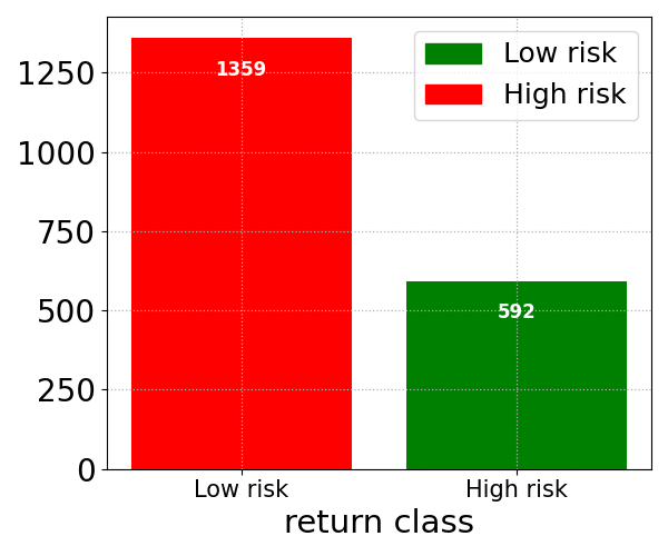
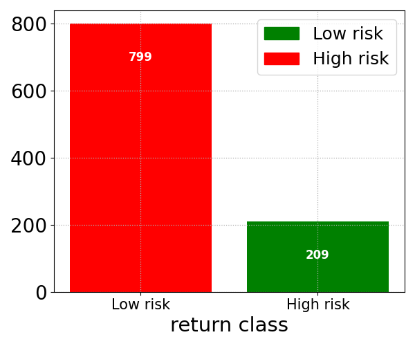
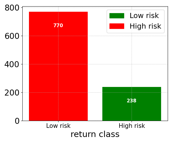
Figures 7(a), 7(b), and 7(c) show the distribution of observations between the two risk classes on the different samples. In the training sample, for example, there is a clear predominance of the low-risk class, which represents approximately 69.66% of the data, compared to only 30.34% for the high-risk class.
This distribution remains relatively similar in the validation and test samples.
Although this distribution is asymmetrical, it does not constitute an extreme imbalance. However, this imbalance remains non-negligible in the context of machine learning, as the majority of classification algorithms implicitly assume a balanced distribution between classes.
This misalignment can significantly impair model performance, particularly when it comes to predicting the minority class, which is often the most critical to identify in real-life applications.
In our case, the minority class corresponds to high-risk situations, whose detection is of great importance for risk management. Misclassification of this class generates much higher costs than for the majority class. It is therefore essential to adopt appropriate strategies to correct for this increased sensitivity to prediction error.
Among existing solutions, data resampling techniques can restore a certain balance between classes. The subsampling approach, which consists in reducing the number of observations in the majority class, proved unsatisfactory in our study, as it generates a significant loss of information and introduces bias in model learning.
In contrast, oversampling methods, in particular the ADASYN (Adaptive Synthetic Sampling) algorithm, have substantially improved performance. By generating new synthetic observations of the minority class, ADASYN enhances the ability of the model to better learn the characteristics of this class while limiting the bias in favor of the dominant class. Although this method implies a longer training time, the trade-off is beneficial for better detection of high-risk cases.
In addition to the Double Deep Q-Network (DDQN), which belongs to the family of deep reinforcement learning algorithms, our study also employs supervised learning techniques such as the Multi-Layer Perceptron (MLP) and the Temporal Convolutional Network (TCN). To address the issue of class imbalance in the dataset, all other supervised learning models are systematically combined with the ADASYN (Adaptive Synthetic Sampling) oversampling technique. This includes traditional models such as Logistic Regression (LR), Support Vector Machines (SVM), and basic neural network architectures such as the Single-Layer Perceptron (ANN).
Another challenge associated with imbalanced classification problems is the selection of appropriate evaluation metrics. Relying solely on accuracy can be misleading: a high accuracy score may simply reflect the model’s tendency to predict the majority class, completely overlooking its ability to identify minority class instances. This is particularly problematic when the minority class carries higher misclassification costs, as is often the case in financial risk prediction. To provide a more reliable and comprehensive evaluation of model performance, we incorporate a set of complementary metrics: the F1-score, which balances precision and recall; recall, which assesses the model’s ability to detect actual positive cases; precision, which measures how many of the predicted positives are true; and the geometric mean (G-mean), which captures the balance between classification performance on both classes.
These metrics offer a more nuanced understanding of the classifiers’ capabilities, especially in skewed class distributions like those in our dataset.
| Metric | LR | SVM | ANN | MLP | TCN | RL |
| Accuracy | 0.616 | 0.639 | 0.618 | 0.719 | 0.788 | 0.835 |
| F1-score | 0.375 | 0.370 | 0.368 | 0.499 | 0.587 | 0.668 |
| Recall | 0.283 | 0.290 | 0.280 | 0.396 | 0.492 | 0.574 |
| Precision | 0.555 | 0.512 | 0.536 | 0.675 | 0.727 | 0.799 |
| G-Mean | 0.489 | 0.494 | 0.485 | 0.596 | 0.672 | 0.735 |
| Metric | LR | SVM | ANN | MLP | TCN | RL |
| Accuracy | 0.514 | 0.524 | 0.530 | 0.678 | 0.720 | 0.794 |
| F1-score | 0.412 | 0.431 | 0.398 | 0.527 | 0.595 | 0.661 |
| Recall | 0.289 | 0.300 | 0.285 | 0.403 | 0.452 | 0.540 |
| Precision | 0.723 | 0.765 | 0.660 | 0.761 | 0.870 | 0.853 |
| G-Mean | 0.492 | 0.508 | 0.485 | 0.602 | 0.653 | 0.714 |
The comparative analysis of the classification models presented in table 5 highlights the outstanding performance of the Temporal Convolutional Network (TCN) and Deep Reinforcement Learning (RL) models, particularly in validation and test samples. Of all the models evaluated, RL stood out as the best performer in all indicators, with an accuracy of 83.5% in validation and 79.4% in test, as well as the best F1-score (0.668 in validation, 0.661 in test). The TCN model also performed well, with an accuracy of 78.8% in validation and 72% in test, just behind the RL model.
In addition, the Recall and G-Mean scores confirm the RL’s robustness, particularly its ability to detect the minority class, which is generally more difficult to classify in unbalanced problems. The RL achieves a Recall of 0.574 in validation and 0.54 in test, the highest values of all the models, which is crucial in a context where misclassification of the high-risk class entails significant costs. The G-Mean, a synthetic indicator that combines precision and recall, corroborates this finding, with 0.735 (validation) and 0.714 (test), reflecting a good balance in the performance of the two classes.
The superiority of RL over TCN and MLP can be explained by the very nature of deep reinforcement learning, which relies on the dynamics of interaction with the environment to enable optimized sequential decision making. Unlike supervised methods such as MLP or TCN, RL learns to maximize a reward function through optimal policies, giving it a strategic advantage in contexts where decisions must take into account time dependency and the future impact of a current prediction. This adaptive capacity, reinforced by mechanisms such as exploration/exploitation and Q-value discounting, enables RL to better manage the uncertainty and temporal structure of financial data.
In short, the key metrics to highlight in this analysis are F1-score, Recall and G-Mean, which provide a comprehensive measure of performance, particularly in the context of unbalanced data. These metrics make it possible to go beyond the limits of accuracy, which is often insufficient in this context, and underline the relevance of using complex models such as RL for financial risk classification tasks.
Now that the analysis of classification models has been completed, our attention turns to the empirical evaluation of the performance of our proposed Value-at-Risk (VaR) model. In order to obtain an accurate and robust VaR estimate, it is essential to use adequate modeling of the conditional volatility dynamics of financial returns, which often exhibit features such as heteroskedasticity, leptokurtosis, and asymmetry.
With this in mind, in addition to the standard GARCH model, we have chosen a GJR-GARCH type conditional volatility structure, which captures the leverage effect, i.e. the tendency of bad news to increase volatility more than good news.
This choice is justified by the asymmetrical nature of financial returns, particularly in equity markets such as the Euro Stoxx 50, where negative shocks have a disproportionate impact on conditional variance. In addition to the dynamic specification of the model, it is imperative to choose an appropriate conditional distribution to model process innovations. Although the normal distribution is a classic choice, it tends to underestimate extreme events due to its thin tails. To overcome this limitation, we explored other fat-tailed distributions and settled on the Student distribution.
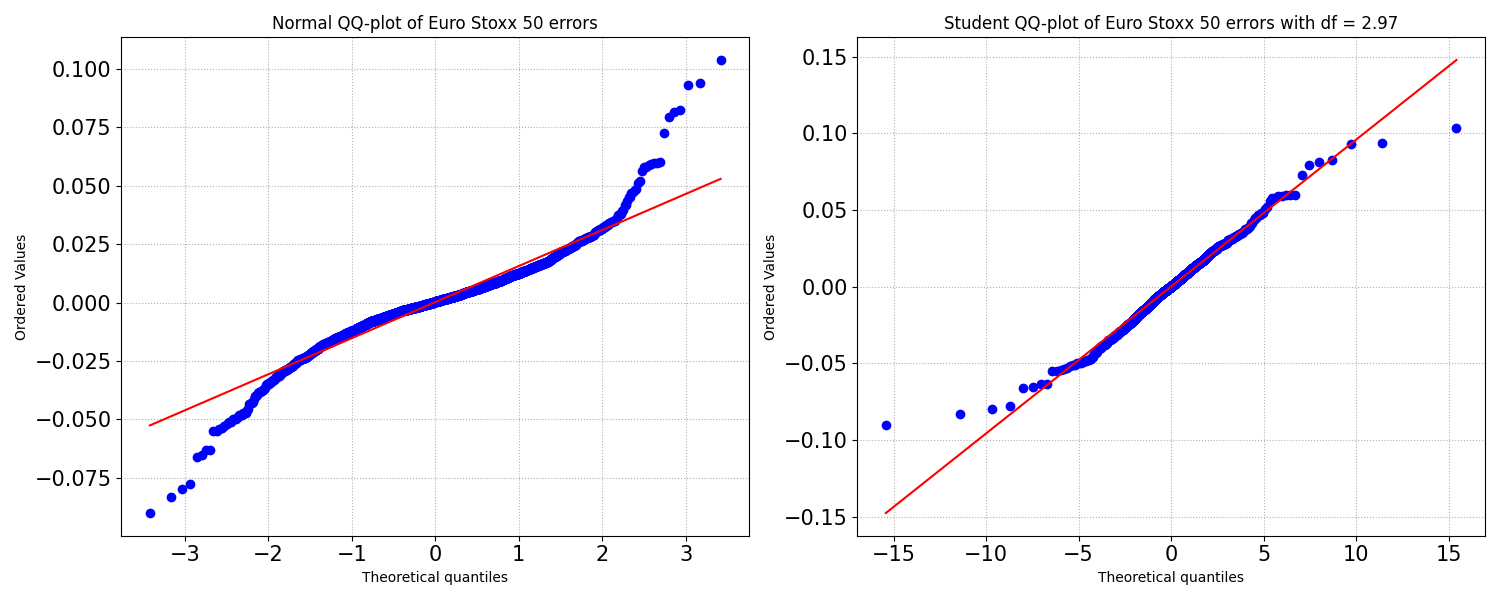
This choice is motivated by the empirical characteristics observed in the distribution of the Euro Stoxx 50 returns, as shown by the statistics presented in table 1, which reveal strong kurtosis and marked asymmetry. These properties are also confirmed by the quantile-quantile plot (QQ plot) illustrated in figure 8, which shows notable deviations from normality, especially in the tails of the distribution.
Thus, the adoption of the Student distribution in our GARCH (resp GJR-GARCH) specification not only better captures extreme risks, but also improves the model’s fit to empirical data. By combining flexible modeling of conditional volatility with a more realistic distribution of returns, our approach aims to provide more accurate VaR estimates that are better adapted to real market conditions.
The analysis of the Value-at-Risk (VaR) models presented in tables 6, 7, and 8 highlights the superior performance of the Reinforcement Learning (RL)-based model, particularly when coupled with the volatility structures GARCH and GJR-GARCH. In table 6, the statistical indicators show that the RL model has better control over the extremes of the distribution, with lower skewness and kurtosis values than the conventional models, indicating a more symmetrical and less leptokurtic distribution. In the test sample, the model has a skewness of -2.048 and a kurtosis of 8.613, significantly lower than the conventional versions, suggesting a better fit to the empirical characteristics of financial returns.
| Model | Version | Min | Median | Mean | Std | Skewness | Kurtosis | Max |
| Original | -0.136 | -0.013 | -0.016 | 0.012 | -5.101 | 35.265 | -0.005 | |
| TCN | -0.129 | -0.010 | -0.014 | 0.012 | -4.747 | 31.630 | -0.004 | |
| RL | -0.138 | -0.010 | -0.014 | 0.011 | -4.929 | 36.258 | -0.004 | |
| Original | -0.148 | -0.013 | -0.016 | 0.012 | -5.436 | 40.562 | -0.005 | |
| TCN | -0.141 | -0.010 | -0.014 | 0.012 | -4.891 | 35.097 | -0.004 | |
| RL | -0.137 | -0.011 | -0.014 | 0.012 | -5.092 | 38.121 | -0.004 | |
| Original | -0.194 | -0.022 | -0.027 | 0.018 | -4.481 | 27.036 | -0.011 | |
| TCN | -0.190 | -0.017 | -0.024 | 0.018 | -4.280 | 25.984 | -0.008 | |
| RL | -0.205 | -0.017 | -0.023 | 0.018 | -4.402 | 29.152 | -0.008 | |
| Original | -0.215 | -0.021 | -0.027 | 0.019 | -4.772 | 31.483 | -0.010 | |
| TCN | -0.210 | -0.017 | -0.024 | 0.019 | -4.350 | 28.127 | -0.007 | |
| RL | -0.204 | -0.018 | -0.023 | 0.019 | -4.534 | 30.670 | -0.007 |
| Model | Version | Min | Median | Mean | Std | Skewness | Kurtosis | Max |
| Original | -0.059 | -0.015 | -0.017 | 0.005 | -2.588 | 13.231 | -0.008 | |
| TCN | -0.071 | -0.014 | -0.015 | 0.007 | -2.118 | 9.694 | -0.005 | |
| RL | -0.069 | -0.013 | -0.015 | 0.006 | -2.048 | 8.613 | -0.005 | |
| Original | -0.054 | -0.015 | -0.017 | 0.006 | -2.033 | 6.564 | -0.007 | |
| TCN | -0.065 | -0.014 | -0.016 | 0.008 | -1.759 | 5.142 | -0.005 | |
| RL | -0.057 | -0.013 | -0.015 | 0.007 | -1.757 | 4.732 | -0.005 | |
| Original | -0.097 | -0.026 | -0.028 | 0.008 | -2.485 | 11.885 | -0.014 | |
| TCN | -0.116 | -0.024 | -0.026 | 0.011 | -2.031 | 8.645 | -0.010 | |
| RL | -0.116 | -0.022 | -0.025 | 0.010 | -2.058 | 8.783 | -0.010 | |
| Original | -0.083 | -0.026 | -0.028 | 0.009 | -1.997 | 6.015 | -0.013 | |
| TCN | -0.100 | -0.023 | -0.026 | 0.013 | -1.723 | 4.754 | -0.010 | |
| RL | -0.096 | -0.022 | -0.025 | 0.011 | -1.773 | 4.874 | -0.010 |
In addition, the medians and means of the VaR series under LR are more conservative, reflecting a conservative estimate of risk, essential for robust risk management decisions. The results in table 7 (Christoffersen test) (Christoffersen, 1998) confirm the statistical validity of the RL model. Unlike conventional (original) models, which are systematically rejected (p-value < 5%), the RL model is accepted in all configurations, in the validation or test sample, and for confidence levels of 5% and 1%. The Christoffersen test, which verifies the correct calibration of VaR violations, thus validates the ability of the RL model to provide forecasts consistent with observed returns.
| Model | Version | Expected | Actual | Test | Test | Test | Decision |
| violations | violations | statistic | critical value | p-value | |||
| Original | 50 | 73 | 9.4259 | 3.8414 | 0.0368 | Reject | |
| TCN | 50 | 72 | 8.6521 | 3.8414 | 0.0032 | Reject | |
| RL | 50 | 52 | 0.0075 | 3.8414 | 0.9310 | Accept | |
| Original | 50 | 68 | 5.8597 | 3.8414 | 0.0154 | Reject | |
| TCN | 50 | 72 | 8.6521 | 3.8414 | 0.0032 | Reject | |
| RL | 50 | 53 | 0.4234 | 3.8414 | 0.5002 | Accept | |
| Original | 10 | 19 | 6.3276 | 3.8414 | 0.0118 | Reject | |
| TCN | 10 | 25 | 13.9951 | 3.8414 | 0.0002 | Reject | |
| RL | 10 | 12 | 0.8288 | 3.8414 | 0.3856 | Accept | |
| Original | 10 | 19 | 6.3276 | 3.8414 | 0.0118 | Reject | |
| TCN | 10 | 24 | 13.9951 | 3.8414 | 0.0002 | Reject | |
| RL | 10 | 11 | 0.0824 | 3.8414 | 0.7741 | Accept |
| Model | Version | Expected | Actual | Test | Test | Test | Decision |
| violations | violations | statistic | critical value | p-value | |||
| Original | 50 | 64 | 3.5722 | 3.8414 | 0.0587 | Accept | |
| TCN | 50 | 47 | 0.2467 | 3.8414 | 0.6193 | Accept | |
| RL | 50 | 52 | 0.0075 | 3.8414 | 0.9310 | Accept | |
| Original | 50 | 64 | 3.5722 | 3.8414 | 0.0587 | Accept | |
| TCN | 50 | 52 | 0.0529 | 3.8414 | 0.8180 | Accept | |
| RL | 50 | 55 | 0.4297 | 3.8414 | 0.5121 | Accept | |
| Original | 10 | 13 | 0.7828 | 3.8414 | 0.3762 | Accept | |
| TCN | 10 | 13 | 0.7828 | 3.8414 | 0.3762 | Accept | |
| RL | 10 | 11 | 0.0823 | 3.8414 | 0.7741 | Accept | |
| Original | 10 | 12 | 0.3481 | 3.8414 | 0.5551 | Accept | |
| TCN | 10 | 10 | 0.0006 | 3.8414 | 0.9797 | Accept | |
| RL | 10 | 11 | 0.0824 | 3.8414 | 0.7741 | Accept |
| Model | Version | Test statistic | Test critical value | Test p-value | Decision |
| Original | 13.4338 | 5.9914 | 0.0012 | Reject | |
| TCN | 10.2577 | 5.9914 | 0.0059 | Reject | |
| RL | 7.6298 | 5.9914 | 0.0320 | Reject | |
| Original | 5.9509 | 5.9914 | 0.0510 | Accept | |
| TCN | 10.2577 | 5.9914 | 0.0059 | Reject | |
| RL | 5.9593 | 5.9914 | 0.0510 | Accept | |
| Original | 7.0584 | 5.9914 | 0.02932 | Reject | |
| TCN | 16.0076 | 5.9914 | 0.0003 | Reject | |
| RL | 4.5624 | 5.9914 | 0.1021 | Accept | |
| Original | 0.9907 | 5.9914 | 0.6093 | Accept | |
| TCN | 15.1671 | 5.9914 | 0.0005 | Reject | |
| RL | 3.4969 | 5.9914 | 0.1740 | Accept |
| Model | Version | Test statistic | Test critical value | Test p-value | Decision |
| Original | 4.5021 | 5.9914 | 0.1052 | Accept | |
| TCN | 0.2660 | 5.9914 | 0.8754 | Accept | |
| RL | 1.3806 | 5.9914 | 0.5014 | Accept | |
| Original | 3.5735 | 5.9914 | 0.1675 | Accept | |
| TCN | 0.2643 | 5.9914 | 0.8761 | Accept | |
| RL | 2.3948 | 5.9914 | 0.3019 | Accept | |
| Original | 1.1229 | 5.9914 | 0.5703 | Accept | |
| TCN | 1.1229 | 5.9914 | 0.5703 | Accept | |
| RL | 4.5624 | 5.9914 | 0.1021 | Accept | |
| Original | 0.6376 | 5.9914 | 0.7270 | Accept | |
| TCN | 0.2012 | 5.9914 | 0.9042 | Accept | |
| RL | 0.3253 | 5.9914 | 0.8498 | Accept |
The TCN model also achieves satisfactory results in the test sample, but less systematically than in RL, particularly in terms of stability on the validation sample.
This performance is reinforced by the results of table 8 (Kupiec test)(Kupiec et al., 1995), which evaluates the suitability of the number of violations with the expected frequency.
Once again, the RL models pass all the tests on the test sample, with p-values well above the critical threshold 5%.
This shows that violations are neither too frequent nor too rare and that they do not present a systematic bias.
The RL model is particularly notable in the and configurations, where it outperforms both the original models and the TCN model. All in all, these results highlight the robustness and accuracy of the RL model, which not only captures market dynamics more realistically through its VaR forecasts, but also meets the rigorous requirements of backtesting tests. The TCN model, while effective in some cases, lags slightly behind in terms of inter-sample stability and overall consistency. RL is therefore the most reliable and efficient model for forecasting extreme risk in volatile financial environments.
4 Discussions
The intrinsic aim of the Value-at-Risk (VaR) model proposed in this study is to correct the recurring biases of traditional models such as GARCH and GJR-GARCH, in particular their tendency to over- or underestimate risk. These models, while robust in their mathematical formulation, have limitations in their ability to adapt dynamically to changing market regimes. These forecasting biases have significant implications for financial institutions, particularly in terms of capital requirements, portfolio management, and regulatory compliance. The use of machine learning, via architectures such as temporal convolutional networks (TCN) and reinforcement learning (RL), aims to dynamically adjust VaR forecasts according to predictive signals from the financial markets, thus improving the model’s sensitivity to real variations in risk. More precisely, the VaR regulation mechanism is based on two parameters, and , which modulate, respectively, the reductions and increases in the initially calculated VaR. In the absence of a universally recognized analytical criterion for their determination, these coefficients were selected by a sensitivity analysis performed on the calibration sample, combined with a rationale for prudent risk management.


The chosen values, and , reflect a desire to penalize false alarms (risk overestimates) more heavily, while maintaining reinforced hedging in the event of risk underestimation by conventional models. Thus, when the classifier anticipates a ’low risk’, the VaR is reduced by 30%, reflecting a unnecessarily tied capital release. In contrast, in the event of high risk, VaR increases by 20%, strengthening prudence in potentially critical periods.
However, the effectiveness of this system depends on the accuracy of the classifier’s predictions. The confusion matrices in figure 9 show that the TCN and RL models significantly outperform the other learning models tested.
The RL model achieved a high number of good classifications, allowing 675 and 597 justified VaR reductions in the validation and test samples, respectively.
At the same time, the TCN model allowed VaR to increase 167 and 203 times, helping to avoid potential breaches of the VaR threshold. These dynamic adjustments result in a better allocation of economic capital, reducing capital requirements without compromising the robustness of risk hedging.
Although some prediction errors remain, notably with the TCN model, which shows a slight increase in the number of VaR violations, these errors have not led to any major failures in risk hedging, as attested by the satisfactory results of backtesting tests (Christoffersen and Kupiec tests). This finding justifies the exclusion of the other machine learning models, which perform less well in classification (see Figures A1 and A2), in the rest of the analysis. Thus, the integration of intelligent classification modules into the VaR calculation process not only makes it possible to refine risk estimates, but above all, to flexibly adapt capital requirements to market conditions.


The proposed model, based on the robust predictions of the TCN and RL classifiers, demonstrates an ability to reconcile statistical rigor and economic efficiency, making it a significant advance in the field of dynamic financial risk management.
The validation and test samples cover the periods from July 7, 2016 to February 3, 2021 and February 4, 2021 to March 13, 2025 respectively, each with 1008 observations corresponding to four years of trading days. These two subperiods, although distinct, share a common feature: high instability in financial markets linked to major exogenous shocks.
The first sample comes at a time of extreme uncertainty marked by the Brexit referendum and, above all, the global health crisis linked to COVID-19. These events profoundly disrupted market dynamics, introducing sudden jumps in volatility, trend breaks, and an increased frequency of systemic shocks. In such an environment, the predictive performance of traditional econometric models, such as GARCH or GJR-GARCH, is often limited by their rigid structure and dependence on stationarity assumptions.
The second sample, although in a post-COVID recovery phase, was nonetheless marked by new sources of instability. Global inflationary pressures, prolonged supply chain disruptions, and Russia’s invasion of Ukraine were all major exogenous shocks that increased uncertainty in European markets. These events generated persistent volatility, often marked by sudden alternations between calm phases and episodes of extreme turbulence.
It is precisely in this context that deep learning models such as the Temporal Convolutional Network (TCN) and the Deep Double Q-Learning Network (DDQN), which is our RL model, show their full potential. TCN, with its ability to capture long-term dependencies via dilated causal convolutions, excels at modeling complex, nonlinear temporal structures. This architecture enables a hierarchical representation of financial signals, offering a better adaptation to the fluctuating volatility regimes characteristic of crisis markets (see Pokou et al., 2024b).
By effectively capturing latent patterns, TCN offers more robust Value-at-Risk (VaR) prediction, reducing under- or overestimation errors.
In this context, the adaptive structure of DDQN is particularly relevant. Unlike purely statistical models, DDQN is based on active learning through interaction with the financial environment. By defining a reward function that incorporates forecast errors and VaR violations, the model dynamically adjusts risk levels, thus anticipating market reversals more effectively. Its ability to dissociate evaluation and target networks also stabilizes learning and avoids overfitting, significantly improving the robustness of the decisions made.
The ability of these models to integrate temporal heterogeneity and risk asymmetry gives them a decisive edge in forecasting extreme measures such as VaR. Their structural flexibility, their ability to capture alternating volatility regimes, and their adaptive learning capacity make them the tools of choice for risk management in ever-changing financial environments, as shown in figure 10.

| Sample | Model | GARCH | TCN | RL |
|
validation |
GARCH 95% | 73 | 72 | 52 |
| GJR 95% | 68 | 72 | 53 | |
| GARCH 99% | 19 | 25 | 12 | |
| GJR 99% | 13 | 13 | 11 | |
|
testing |
GARCH 95% | 64 | 47 | 52 |
| GJR 95% | 64 | 52 | 55 | |
| GARCH 99% | 13 | 13 | 11 | |
| GJR 99% | 12 | 10 | 11 |
The empirical results of the backtesting, presented in Tables 7 and 8, confirm these strengths: The TCN and DDQN models almost systematically meet the specified confidence thresholds (95% and 99%), while satisfying the Kupiec (unconditional coverage) and Christoffersen (independence of violations) tests. These results illustrate the superiority of machine learning-based approaches, particularly in periods of structurally unstable volatility.
To assess the robustness of the different VaR forecasting models, table 4 summarizes the number of violations observed for all the approaches tested, whether traditional models (GARCH, GJR-GARCH) or machine learning methods (notably TCN and RL), taking into account both the two volatility structures considered and the usual risk thresholds (1% and 5%). This table highlights the differential performance of the models in terms of hedging accuracy, in particular their ability to minimize occurrences of theoretical VaR overshoot. These empirical results are visually confirmed by the violation distributions shown as boxplots in figure 4. However, to go beyond a simple descriptive analysis and guarantee the statistical validity of the observed deviations, a nonparametric Wilcoxon test was applied. The results, presented in table 10, confirm that the RL model shows a significantly lower average number of violations than all other models, at a significance level of 5%.
| Test hypotheses | Test indicators | TCN vs GARCH | RL vs GARCH | TCN vs RL |
| : vs : | Test statistic | 12 | 0.0 | 8 |
| P-value | 0.3997 | 0.0039 | 0.0976 |
With a p-value of 0.0039, we have strong statistical evidence to conclude that the reinforcement learning (RL) model generates significantly fewer Value-at-Risk (VaR) violations than the GARCH model, under equivalent conditions of volatility and risk thresholds. This result indicates a better performance of the RL model in terms of extreme risk management, which can be interpreted as a greater ability to anticipate and limit exceptional losses. Compared to the TCN (Temporal Convolutional Network) model, the RL model also tends to produce a lower number of violations, but the difference does not reach the conventional statistical significance threshold of 5%.
| GARCH | GJR-GARCH | ||||
| Ind stat | TCN | RL | TCN | RL | |
| 5% | statistic | 243568 | 228198 | 241408 | 235833 |
| p-value | 0.1236 | 0.0136 | 0.08212 | 0.02308 | |
| 1% | statistic | 252784 | 238663 | 241376 | 236536 |
| p-value | 0.4362 | 0.04572 | 0.08159 | 0.0436 | |
| GARCH | GJR-GARCH | ||||
| Ind stat | TCN | RL | TCN | RL | |
| 5% | statistic | 234618 | 226652 | 220530 | 235833 |
| p-value | 0.01678 | 0.0014 | 0.0001 | 0.02308 | |
| 1% | statistic | 237250 | 236431 | 238642 | 238250 |
| p-value | 0.03284 | 0.02685 | 0.0455 | 0.04159 | |
From the point of view of efficient regulatory capital management, it is essential that Value-at-Risk (VaR) models are not only accurate in terms of covering extreme losses but also conservative without being excessively penalizing.
In particular, this means that, where market conditions allow, proposed models should produce less stringent VaR estimates while maintaining an acceptable frequency of violation.
In other words, a high-performance model is one that reduces capital requirements while respecting regulatory risk thresholds. In order to assess the ability of machine learning models to meet this objective, we compared the distribution of VaR values generated by the TCN and RL models to those derived from traditional conditional volatility-based models, such as GARCH and GJR-GARCH. More specifically, Figures 12 and 13 superimpose the empirical distributions of the values derived from a GJR-GARCH model with those of the values predicted, respectively, by the TCN and RL models, for the risk thresholds and .


A visual inspection of these distributions shows that, in the majority of cases, the distributions resulting from machine learning models are shifted to the right, i.e. their values are less negative in comparison with traditional models.
This shift suggests a potential reduction in the capital required to cover extreme losses.
To statistically confirm this observation, we use the nonparametric Mann-Whitney test (Mann and Whitney, 1947), which tests the hypothesis that the median of the VaR distribution of machine learning models is higher than that from the GARCH or GJR-GARCH models.
The choice of the median, rather than the mean, is justified by its robustness to extreme values, particularly frequent in the left tail of financial return distributions.
In our case, given that all VaR values are negative, a less negative median (i.e. higher in absolute value) implies a lower capital allocation, provided hedging remains sufficient.
The test results, presented in table 11, confirm that the medians of the distributions are statistically superior to those of the GARCH-type models, for both samples (validation and test), regardless of the risk threshold (1% or 5%) and the volatility specification used.
In contrast, the results for the TCN model show that its performance is more nuanced. In the validation sample, only one configuration (5% GARCH) leads to a significant difference in the median.
However, in the test sample, the differences are significant at all thresholds and for both types of volatility model, but with a smaller magnitude than that observed for the RL.
These results suggest that not only are deep learning models in particular the reinforcement model (RL) able to better anticipate VaR violations, but they also do so in a more capital-efficient way. This reinforces their relevance for dynamic risk management, where adaptability to the market environment is crucial.
The financial crisis of 2007-2009 highlighted the many weaknesses in the risk management models used by financial institutions, particularly those based on Value-at-Risk (VaR), which had proved insufficient to anticipate or absorb extreme events. In response, the Basel Committee on Banking Supervision undertook a series of major reforms (Supervision, 2011, 2012; on Banking Supervision, 2017), known as Basel III, one of the most notable of which was the gradual replacement of VaR by a new, more conservative and robust risk measure. Expected Shortfall (ES). Unlike VaR, which evaluates the maximum potential loss at a certain confidence level without providing information on losses beyond this threshold, Expected Shortfall measures the conditional average loss in the event of VaR being exceeded. Mathematically, it is expressed as follows:
In other words, the expected shortfall is directly related to VaR insofar as it is based on knowledge of the latter.
Thus, building a robust VaR model remains an essential prerequisite to estimating the expected shortfall, especially when modeling distribution tails in a context of strong asymmetries and conditional volatility.
In this sense, even if VaR is no longer a central regulatory measure, it remains a fundamental component of the risk calculation chain.
In this context, our approach is fully in line with current risk management concerns.
Indeed, we propose VaR estimation using deep learning models, notably the Temporal Convolutional Network (TCN) and Reinforcement Learning (RL) architectures, capable of better capturing the complex temporal dynamics of financial series.
These models differ from traditional parametric approaches in their ability to incorporate a large historical memory, to learn about nonlinear relationships between variables, and to adapt to changing market regimes.
The use of TCN, for example, enables efficient handling of long-time dependencies while retaining a convolutional structure that facilitates parallelization and speeds up training compared to conventional RNNs. As for the RL model, it introduces a dynamic optimization dimension, by learning a policy that maximizes a reward associated with the correct VaR estimate, which is particularly relevant in an active risk management framework.
However, these models also have certain limitations. Their implementation requires a relatively long calibration phase, high sensitivity to hyperparameters, and advanced algorithmic expertise. In addition, their interpretability may be less than that of traditional models, which can be a hindrance in regulatory contexts that require a clear justification for decisions. These considerations, while essential from an operational perspective, will not be addressed in depth in the present work, which focuses on the empirical evaluation of predictive performance. Ultimately, by proposing an improved model of VaR, this work provides a solid basis for estimating Expected Shortfall, while contributing to contemporary debates on the integration of artificial intelligence techniques into risk management systems. The relevance of VaR therefore remains intact, not only as a standalone tool but also as a methodological foundation for more advanced measures in line with current regulatory standards.
5 Conclusion
This paper introduced a novel methodology for Value-at-Risk (VaR) estimation designed to reduce both the number of risk violations and the capital reserves required for market risk coverage. The core innovation lies in the dynamic adjustment of the VaR level based on a predictive classification of return risk, allowing for more conservative thresholds during turbulent periods and less stringent capital constraints during calmer market regimes.
To achieve this, we reformulated the problem of return forecasting into an imbalanced classification task a well-known challenge in financial time series modeling due to the inherent asymmetry and rarity of extreme events.
Addressing this complexity, we leveraged the Double Deep Q-Network (DDQN), a reinforcement learning algorithm grounded in deep learning architectures. Unlike traditional classifiers, DDQN learns an optimal policy for decision making under uncertainty, enabling it to handle temporal dependencies and adapt its classification strategy based on past prediction errors and changing market conditions.
Empirical results show that the VaR forecasts produced by our DDQN-based approach consistently outperform those of benchmark models in terms of backtest performance and capital efficiency. Furthermore, the ability of the model to anticipate changes in market risk by learning from its environment through reward-based feedback confers a strategic advantage in dynamic risk management.
Our contribution is twofold. First, we advance the econometric literature on risk measures by proposing an AI-enhanced VaR model capable of adaptive behavior in volatile financial environments. Second, we contribute to the broader field of data science by demonstrating the effectiveness of reinforcement learning, and specifically DDQN, in solving imbalanced classification problems in the context of financial time series.
Future work may explore the integration of alternative reinforcement learning paradigms and further refine model calibration techniques to enhance interpretability and computational efficiency, an important consideration, given the model’s parametric complexity and training time, which we acknowledge as a limitation not addressed in the present study.
Compliance with Ethical Standards
Declaration of Competing Interest
All authors declare that they have no conflicts of interest.
Ethical approval:
This article does not contain any studies with human participants or animals performed by any of the authors.
References
- Alostad and Davulcu (2017) H. Alostad and H. Davulcu. Directional prediction of stock prices using breaking news on twitter. In Web Intelligence, volume 15, pages 1–17. IOS Press, 2017.
- Ampomah et al. (2020) E. K. Ampomah, Z. Qin, and G. Nyame. Evaluation of tree-based ensemble machine learning models in predicting stock price direction of movement. Information, 11(6):332, 2020.
- Barandela et al. (2004) R. Barandela, R. M. Valdovinos, J. S. Sánchez, and F. J. Ferri. The imbalanced training sample problem: Under or over sampling? In Structural, Syntactic, and Statistical Pattern Recognition: Joint IAPR International Workshops, SSPR 2004 and SPR 2004, Lisbon, Portugal, August 18-20, 2004. Proceedings, pages 806–814. Springer, 2004.
- Barrera et al. (2022) D. Barrera, S. Crépey, E. Gobet, H.-D. Nguyen, and B. Saadeddine. Learning value-at-risk and expected shortfall. 2022.
- Becker and Leschinski (2018) J. Becker and C. Leschinski. Directional predictability of daily stock returns. Technical report, Hannover Economic Papers (HEP), 2018.
- Bollerslev (1986) T. Bollerslev. Generalized autoregressive conditional heteroskedasticity. Journal of econometrics, 31(3):307–327, 1986.
- Chandrasekara et al. (2019) V. Chandrasekara, C. Tilakaratne, and M. Mammadov. An improved probabilistic neural network model for directional prediction of a stock market index. Applied Sciences, 9(24):5334, 2019.
- Chawla et al. (2002) N. V. Chawla, K. W. Bowyer, L. O. Hall, and W. P. Kegelmeyer. Smote: synthetic minority over-sampling technique. Journal of artificial intelligence research, 16:321–357, 2002.
- Christoffersen (1998) P. F. Christoffersen. Evaluating interval forecasts. International economic review, pages 841–862, 1998.
- Chung and Hong (2007) J. Chung and Y. Hong. Model-free evaluation of directional predictability in foreign exchange markets. Journal of Applied Econometrics, 22(5):855–889, 2007.
- Clements et al. (2019) W. R. Clements, B. Van Delft, B.-M. Robaglia, R. B. Slaoui, and S. Toth. Estimating risk and uncertainty in deep reinforcement learning. arXiv preprint arXiv:1905.09638, 2019.
- Deng et al. (2016) Y. Deng, F. Bao, Y. Kong, Z. Ren, and Q. Dai. Deep direct reinforcement learning for financial signal representation and trading. IEEE transactions on neural networks and learning systems, 28(3):653–664, 2016.
- Dixit (1990) A. K. Dixit. Optimization in economic theory. Oxford University Press, USA, 1990.
- Dreiseitl and Ohno-Machado (2002) S. Dreiseitl and L. Ohno-Machado. Logistic regression and artificial neural network classification models: a methodology review. Journal of biomedical informatics, 35(5-6):352–359, 2002.
- Elhassan and Aljurf (2016) T. Elhassan and M. Aljurf. Classification of imbalance data using tomek link (t-link) combined with random under-sampling (rus) as a data reduction method. Global J Technol Optim S, 1:2016, 2016.
- Fama (1970) E. F. Fama. Efficient capital markets: A review of theory and empirical work. The journal of Finance, 25(2):383–417, 1970.
- Fawcett and Provost (1997) T. Fawcett and F. Provost. Adaptive fraud detection. Data mining and knowledge discovery, 1(3):291–316, 1997.
- Gilks et al. (1995) W. R. Gilks, S. Richardson, and D. Spiegelhalter. Markov chain Monte Carlo in practice. CRC press, 1995.
- Glosten et al. (1993) L. R. Glosten, R. Jagannathan, and D. E. Runkle. On the relation between the expected value and the volatility of the nominal excess return on stocks. The journal of finance, 48(5):1779–1801, 1993.
- Goodfellow et al. (2016) I. Goodfellow, Y. Bengio, A. Courville, and Y. Bengio. Deep learning, volume 1. MIT press Cambridge, 2016.
- Gu et al. (2017) S. Gu, E. Holly, T. Lillicrap, and S. Levine. Deep reinforcement learning for robotic manipulation with asynchronous off-policy updates. In 2017 IEEE international conference on robotics and automation (ICRA), pages 3389–3396. IEEE, 2017.
- Han et al. (2005) H. Han, W.-Y. Wang, and B.-H. Mao. Borderline-smote: a new over-sampling method in imbalanced data sets learning. In International conference on intelligent computing, pages 878–887. Springer, 2005.
- Jang et al. (2019) B. Jang, M. Kim, G. Harerimana, and J. W. Kim. Q-learning algorithms: A comprehensive classification and applications. IEEE access, 7:133653–133667, 2019.
- Kanas (2001) A. Kanas. Neural network linear forecasts for stock returns. International Journal of Finance & Economics, 6(3):245–254, 2001.
- Kotsiantis et al. (2006) S. Kotsiantis, D. Kanellopoulos, P. Pintelas, et al. Handling imbalanced datasets: A review. GESTS international transactions on computer science and engineering, 30(1):25–36, 2006.
- Kupiec et al. (1995) P. H. Kupiec et al. Techniques for verifying the accuracy of risk measurement models, volume 95. Division of Research and Statistics, Division of Monetary Affairs, Federal …, 1995.
- Kursa and Rudnicki (2010) M. B. Kursa and W. R. Rudnicki. Feature selection with the boruta package. Journal of statistical software, 36:1–13, 2010.
- Kursa et al. (2010) M. B. Kursa, A. Jankowski, and W. R. Rudnicki. Boruta–a system for feature selection. Fundamenta Informaticae, 101(4):271–285, 2010.
- Lea et al. (2016) C. Lea, R. Vidal, A. Reiter, and G. D. Hager. Temporal convolutional networks: A unified approach to action segmentation. In Computer Vision–ECCV 2016 Workshops: Amsterdam, The Netherlands, October 8-10 and 15-16, 2016, Proceedings, Part III 14, pages 47–54. Springer, 2016.
- Linton and Whang (2007) O. Linton and Y.-J. Whang. The quantilogram: With an application to evaluating directional predictability. Journal of Econometrics, 141(1):250–282, 2007.
- Liu et al. (2020) X.-Y. Liu, H. Yang, Q. Chen, R. Zhang, L. Yang, B. Xiao, and C. D. Wang. Finrl: A deep reinforcement learning library for automated stock trading in quantitative finance. arXiv preprint arXiv:2011.09607, 2020.
- Mann and Whitney (1947) H. B. Mann and D. R. Whitney. On a test of whether one of two random variables is stochastically larger than the other. The annals of mathematical statistics, pages 50–60, 1947.
- Mao et al. (2016) H. Mao, M. Alizadeh, I. Menache, and S. Kandula. Resource management with deep reinforcement learning. In Proceedings of the 15th ACM workshop on hot topics in networks, pages 50–56, 2016.
- Markowitz (1952) H. Markowitz. Portfolio selection. Journal of Finance, 1952.
- Markowitz (1959) H. M. Markowitz. Portfolio selection: E cient diversification of investments. Cowles Foundation Monograph, 16, 1959.
- Mnih et al. (2013) V. Mnih, K. Kavukcuoglu, D. Silver, A. Graves, I. Antonoglou, D. Wierstra, and M. Riedmiller. Playing atari with deep reinforcement learning. arXiv preprint arXiv:1312.5602, 2013.
- Morimura et al. (2012) T. Morimura, M. Sugiyama, H. Kashima, H. Hachiya, and T. Tanaka. Parametric return density estimation for reinforcement learning. arXiv preprint arXiv:1203.3497, 2012.
- Murtagh (1991) F. Murtagh. Multilayer perceptrons for classification and regression. Neurocomputing, 2(5-6):183–197, 1991.
- Nevasalmi (2020) L. Nevasalmi. Forecasting multinomial stock returns using machine learning methods. The Journal of Finance and Data Science, 6:86–106, 2020.
- Nyberg (2011) H. Nyberg. Forecasting the direction of the us stock market with dynamic binary probit models. International Journal of Forecasting, 27(2):561–578, 2011.
- Oh and Sheng (2011) C. Oh and O. Sheng. Investigating predictive power of stock micro blog sentiment in forecasting future stock price directional movement. 2011.
- on Banking Supervision (2017) B. C. on Banking Supervision. Basel iii: Finalising post-crisis reforms. Bank for International Settlements, 2017.
- Pereira et al. (2020) R. M. Pereira, Y. M. Costa, and C. N. Silla Jr. Mltl: A multi-label approach for the tomek link undersampling algorithm. Neurocomputing, 383:95–105, 2020.
- Pokou et al. (2024a) F. Pokou, J. S. Kamdem, and F. Benhmad. Deep reinforcement learning for an empirical approach to value-at-risk. 2024a.
- Pokou et al. (2024b) F. Pokou, J. Sadefo Kamdem, and F. Benhmad. Hybridization of arima with learning models for forecasting of stock market time series. Computational Economics, 63(4):1349–1399, 2024b.
- Pokou (2022) F. V. M. Pokou. Une contribution sur l’allocation ou la prévision d’actifs d’un portefeuille. PhD thesis, Université de Montpellier, 2022.
- Puterman (2014) M. L. Puterman. Markov decision processes: discrete stochastic dynamic programming. John Wiley & Sons, 2014.
- Rosenblatt (1958) F. Rosenblatt. The perceptron: a probabilistic model for information storage and organization in the brain. Psychological review, 65(6):386, 1958.
- Sunny et al. (2020) M. A. I. Sunny, M. M. S. Maswood, and A. G. Alharbi. Deep learning-based stock price prediction using lstm and bi-directional lstm model. In 2020 2nd novel intelligent and leading emerging sciences conference (NILES), pages 87–92. IEEE, 2020.
- Supervision (2011) B. Supervision. Basel committee on banking supervision. Principles for Sound Liquidity Risk Management and Supervision (September 2008), 2011.
- Supervision (2012) B. Supervision. Basel committee on banking supervision. 2012.
- Sutton and Barto (1998) R. Sutton and A. Barto. Reinforcement learning: An introduction. IEEE Transactions on Neural Networks, 9(5):1054–1054, 1998.
- Sutton (1988) R. S. Sutton. Learning to predict by the methods of temporal differences. Machine learning, 3:9–44, 1988.
- Szepesvári (2010) C. Szepesvári. Value prediction problems. In Algorithms for Reinforcement Learning, pages 11–36. Springer, 2010.
- Tang et al. (2008) Y. Tang, Y.-Q. Zhang, N. V. Chawla, and S. Krasser. Svms modeling for highly imbalanced classification. IEEE Transactions on Systems, Man, and Cybernetics, Part B (Cybernetics), 39(1):281–288, 2008.
- Tealab (2018) A. Tealab. Time series forecasting using artificial neural networks methodologies: A systematic review. Future Computing and Informatics Journal, 3(2):334–340, 2018.
- Van Hasselt et al. (2016) H. Van Hasselt, A. Guez, and D. Silver. Deep reinforcement learning with double q-learning. In Proceedings of the AAAI conference on artificial intelligence, volume 30, 2016.
- Vapnik (1999) V. Vapnik. The nature of statistical learning theory. Springer science & business media, 1999.
- Watkins (1989) C. J. C. H. Watkins. Learning from delayed rewards. 1989.
- White III and White (1989) C. C. White III and D. J. White. Markov decision processes. European Journal of Operational Research, 39(1):1–16, 1989.
- Yang et al. (2020) H. Yang, X.-Y. Liu, S. Zhong, and A. Walid. Deep reinforcement learning for automated stock trading: An ensemble strategy. In Proceedings of the first ACM international conference on AI in finance, pages 1–8, 2020.
- Ying et al. (2022) C. Ying, X. Zhou, H. Su, D. Yan, N. Chen, and J. Zhu. Towards safe reinforcement learning via constraining conditional value-at-risk. arXiv preprint arXiv:2206.04436, 2022.
- Yu et al. (2021) C. Yu, J. Liu, S. Nemati, and G. Yin. Reinforcement learning in healthcare: A survey. ACM Computing Surveys (CSUR), 55(1):1–36, 2021.
- Zeng et al. (2016) M. Zeng, B. Zou, F. Wei, X. Liu, and L. Wang. Effective prediction of three common diseases by combining smote with tomek links technique for imbalanced medical data. In 2016 IEEE International Conference of Online Analysis and Computing Science (ICOACS), pages 225–228. IEEE, 2016.
- Zhang (2003) G. P. Zhang. Time series forecasting using a hybrid arima and neural network model. Neurocomputing, 50:159–175, 2003.
- Zhang and Li (2014) H. Zhang and M. Li. Rwo-sampling: A random walk over-sampling approach to imbalanced data classification. Information Fusion, 20:99–116, 2014.
- Zhang et al. (2020) Z. Zhang, S. Zohren, and R. Stephen. Deep reinforcement learning for trading. The Journal of Financial Data Science, 2020.
- Zhao et al. (2017) X. Zhao, L. Zhang, L. Xia, Z. Ding, D. Yin, and J. Tang. Deep reinforcement learning for list-wise recommendations. arXiv preprint arXiv:1801.00209, 2017.
Appendix A Confusion matrices


Appendix B Selected features
| no | Asset | ID | Informations |
| 1 | AEX | ∧AEX | Index |
| 2 | CAC 40 | ∧FCHI | Index |
| 3 | DAX | ∧GDAXI | Index |
| 4 | Euro Stoxx 50 | ∧STOXX50E | Index |
| 5 | Brent Crude Oil Last Day | BZ=F | Commodity |
| 6 | EURO/USD | EURUSD=X | Currency |
| 7 | EURO/GBP | EURGBP=X | Currency |
| 8 | SPDR EURO STOXX 50 ETF | FEZ | ETF |
| 9 | Bollinger Bands | BB upper & BB lower | Technical trading indicator |
| 10 | Relative Strength Index | RSI 14 | Technical trading indicator |
| 11 | Standard Moving Average | SMA 5 & SMA 15 | Technical trading indicator |
| 12 | Exponentially Weighted Moving Average | EMA 5 & EMA 15 | Technical trading indicator |
| 13 | Forecasting returns using GARCH model | STOXX50E mu GARCH | Econometric indicators |
| 14 | Forecasting volatility using GARCH model | STOXX50E sig GARCH | Econometric indicators |
| 15 | Forecasting volatility using GJR6GARCH model | STOXX50E sig gjr-GARCH | Econometric indicators |
| 16 | Forecasting VaR using GARCH model | ∧STOXX50E VaR GARCH | Econometric indicators |
| 17 | Forecasting VaR using GJR-GARCH model | ∧STOXX50E VaR gjr-GARCH | Econometric indicators |
| 18 | SMA strategy trading positions | Signal 1 | Technical trading indicator |
| 19 | EMA strategy trading positions | Signal 2 | Technical trading indicator |
| 20 | BB strategy trading positions | Signal 3 | Technical trading indicator |
| 21 | Forecasting risk level of returns with ARIMA model | ARIMA indicator | Class prediction |
