跳到论文正文
W Papers独立论文阅读器 arXiv:2503.21855 论文正文 计算阅读时间 · 0%
引用这篇论文根据当前论文元数据生成,正式投稿前建议核对。


11footnotetext: Université de Genève, Section de mathématiques, Genève, Switzerland. Eugen.Bronasco@unige.ch.22footnotetext: Univ Rennes, INRIA (Research team MINGuS), IRMAR (CNRS UMR 6625) and ENS Rennes, France. Adrien.Busnot-Laurent@inria.fr, Baptiste.Huguet@math.cnrs.fr.

High order integration of stochastic dynamics on Riemannian manifolds with frozen flow methods

Eugen Bronasco1, Adrien Busnot Laurent2 and Baptiste Huguet2
Abstract

We present a new class of numerical methods for solving stochastic differential equations with additive noise on general Riemannian manifolds with high weak order of accuracy. In opposition to the popular approach with projection methods, the proposed methods are intrinsic: they only rely on geometric operations and avoid coordinates and embeddings. We provide a robust and general convergence analysis and an algebraic formalism of exotic planar Butcher series for the computation of order conditions at any high order. To illustrate the methodology, an explicit method of second weak order is introduced, and several numerical experiments confirm the theoretical findings and extend the approach for the sampling of the invariant measure of Riemannian Langevin dynamics.

Keywords:  geometric numerical integration, stochastic differential equations, Riemannian manifolds, Riemannian Langevin, ergodicity, Lie-group methods, frozen flow, Butcher series, exotic series, post-Lie algebra, Hopf algebra, order conditions.

AMS subject classification (2020):  16T05, 41A58, 60H35, 37M25, 65L06, 70H45.

1 Introduction

Let (ℳ,g)(\mathcal{M},g) be a smooth connected complete Riemannian manifold equipped with a metric gg and its Levi-Civita connection ∇\nabla. Let E1E_{1},…,EDE_{D} be a frame, that is, DD smooth vector fields with dim(ℳ)≤D\dim(\mathcal{M})\leq D such that

Spanℝ⁡(E1​(y),…,ED​(y))=Ty​ℳ,y∈ℳ.\operatorname{Span}_{\mathbb{R}}(E_{1}(y),\dots,E_{D}(y))=T_{y}\mathcal{M},\quad y\in\mathcal{M}.

Given a smooth vector field F​(x)=∑d=1Dfd​(x)​Ed​(x)F(x)=\sum_{d=1}^{D}f^{d}(x)E_{d}(x), we consider Stratonovich stochastic differential equations on ℳ\mathcal{M} of the form,

d​X​(t)=F​(X​(t))​d​t+2​∑d=1DEd​(X​(t))∘d​Wd​(t).dX(t)=F(X(t))dt+\sqrt{2}\sum_{d=1}^{D}E_{d}(X(t))\circ dW_{d}(t). (1.1)

Equation (1.1) can be seen as a stochastic differential equation with additive noise w.r.t. the frame (Ed)(E_{d}). Under reasonable assumptions, the flow of (1.1) is well-posed on ℳ\mathcal{M}. The aim of the present paper is to introduce a new class of intrinsic one-step integrators

Xn+1=Φh​(Xn),X_{n+1}=\Phi_{h}(X_{n}), (1.2)

where Φh\Phi_{h} is a (random) local diffeomorphism of ℳ\mathcal{M} for a timestep hh small enough, for solving dynamics of the form (1.1) with high order of accuracy in the weak sense. We take inspiration from Lie-group integrators [70, 77, 71, 72, 47, 73] and more precisely from Crouch-Grossman and commutator-free methods [29, 82, 25, 81]. In opposition to [64], we consider an approach with frames allowing us to define a new versatile class of methods that works on any smooth Riemannian manifold. An important feature of the new integrators is that they do not rely on the use of embeddings or on local coordinates. Their formulation, convergence analysis, order theory, and implementation are entirely intrinsic.

It is crucial that a numerical approximation respects the geometry of the problem and lies on ℳ\mathcal{M}, especially for the sampling of measures. In particular, our methods extend naturally for the sampling of measures interpreted as invariant measure of ergodic dynamics. Let us consider for instance the central example from molecular dynamics of Riemannian Langevin dynamics:

d​X​(t)\displaystyle dX(t) =−∑d=1D(Ed​[V]​Ed+∇EdEd)​(X​(t))​d​t+2​∑d=1DEd​(X​(t))∘d​Wd​(t)\displaystyle=-\sum_{d=1}^{D}(E_{d}[V]E_{d}+\nabla_{E_{d}}E_{d})(X(t))dt+\sqrt{2}\sum_{d=1}^{D}E_{d}(X(t))\circ dW_{d}(t) (1.3)
=−∇V​(X​(t))​d​t+2​d​Bℳ​(t),\displaystyle=-\nabla V(X(t))dt+\sqrt{2}dB_{\mathcal{M}}(t),

where VV is a smooth potential, the frame (Ed)(E_{d}) is an orthonormal frame basis, and the vector field F=−∇V−∑∇EdEdF=-\nabla V-\sum\nabla_{E_{d}}E_{d} contains the Itô correction. Note that the choice V=0V=0 yields Brownian dynamics Bℳ​(t)B_{\mathcal{M}}(t) on ℳ\mathcal{M}. Riemannian Langevin dynamics (1.3) are naturally ergodic under mild assumptions, that is, the dynamics in long time behaves according to a deterministic probability measure, called the invariant measure, which takes the explicit form d​μ∞=e−V​d​vold\mu_{\infty}=e^{-V}d\operatorname{vol}. The generator of the SDE is ℒ=−∇V⋅∇+Δg\mathcal{L}=-\nabla V\cdot\nabla+\Delta_{g}, where Δg\Delta_{g} is the Laplace-Beltrami operator. Actually, an integrator of weak order pp automatically has at least order pp for the invariant measure [88]. We refer for instance to [33] and references therein for appropriate assumptions to obtain the ergodicity of a numerical scheme in the context of dynamics in ℝd\mathbb{R}^{d}. To the best of our knowledge, there does not exist any intrinsic method of order greater than one for sampling the invariant measure of Riemannian Langevin dynamics.

There exists a handful of extrinsic stochastic integrators on manifolds, that is, integrators that rely on an embedding of ℳ\mathcal{M} in a Euclidean space of higher dimension. In the case of smooth embedded manifolds ℳ={x∈ℝD,ζ​(x)=0}\mathcal{M}=\{x\in\mathbb{R}^{D},\zeta(x)=0\} defined by constraints, the approach using projection methods is the most popular in the literature (see [60] and references therein). We cite in particular the constrained Euler method:

Xn+1=Xn+h​F​(Xn)+2​h​ξn+λn​∇ζ​(Xn),ζ​(Xn+1)=0,X_{n+1}=X_{n}+hF(X_{n})+\sqrt{2h}\xi_{n}+\lambda_{n}\nabla\zeta(X_{n}),\quad\zeta(X_{n+1})=0,

where λn\lambda_{n} is a Lagrange multiplier and the ξn\xi_{n} are independent standard Gaussian random vectors. While the approach using projection methods is straightforward to implement and widely used in applications, these methods rely on an embedding of ℳ\mathcal{M} into a vector space of much higher dimension and use non-intrinsic quantities, so that they often face severe timestep restrictions. Moreover, the algebraic structure associated to order theory is difficult and does not allow at the present time for the creation of methods of arbitrarily high order, nor for a systematic approach to stochastic backward error analysis [15]. Stochastic Lie group methods seldom appear in the literature [64, 31, 65, 3, 66, 28], but focus on low order approximations on specific manifolds (typically variants of Lie-Euler on the sphere), with an extrinsic convergence analysis, and no high order theory. In the recent work [10], a new approach for sampling (1.3) is developed using the following intrinsic integrator, called Riemannian Langevin method

Xn+1=expRiem⁡(−h​∇V​(Xn)+2​h​ξn+1)​Xn,X_{n+1}=\exp^{\text{Riem}}(-h\nabla V(X_{n})+\sqrt{2h}\xi_{n+1})X_{n},

where expRiem\exp^{\text{Riem}} is the geodesic exponential for the Levi-Civita connection ∇\nabla. This method has order one for solving (1.3) in the weak sense and for the invariant measure. One could be tempted to say that such a method is exact for V=0V=0, but it still has only order one, in contrast to the Euclidean setting where it is exact in law.

We introduce the first intrinsic methods of high weak order for solving (1.1) using only evaluations of FF and the frame. In particular, we highlight the following new explicit integrator of second weak order for solving (1.1), and using the minimal number of evaluations of FF per step:

Hn\displaystyle H_{n} =exp⁡(∑d=1D(12​h​fd​(Xn)+h​ξnd,1)​Ed)​Xn\displaystyle=\exp\bigg{(}\sum_{d=1}^{D}\Big{(}\frac{1}{2}hf^{d}(X_{n})+\sqrt{h}\xi^{d,1}_{n}\Big{)}E_{d}\bigg{)}X_{n}
Xn+1\displaystyle X_{n+1} =exp⁡(∑d=1D((22−1)​h​fd​(Xn)+(2−2)​h​fd​(Hn)+(1−2)​h​ξnd,1+h​ξnd,2)​Ed)\displaystyle=\exp\bigg{(}\sum_{d=1}^{D}\Big{(}\big{(}\frac{\sqrt{2}}{2}-1\big{)}hf^{d}(X_{n})+(2-\sqrt{2})hf^{d}(H_{n})+\big{(}1-\sqrt{2}\big{)}\sqrt{h}\xi^{d,1}_{n}+\sqrt{h}\xi^{d,2}_{n}\Big{)}E_{d}\bigg{)}
exp⁡(∑d=1D((1−22)​h​fd​(Xn)+(2−1)​h​fd​(Hn)+2​h​ξnd,1)​Ed)​Xn.\displaystyle\exp\bigg{(}\sum_{d=1}^{D}\Big{(}\big{(}1-\frac{\sqrt{2}}{2}\big{)}hf^{d}(X_{n})+(\sqrt{2}-1)hf^{d}(H_{n})+\sqrt{2h}\xi^{d,1}_{n}\Big{)}E_{d}\bigg{)}X_{n}.

where the ξnd,l\xi^{d,l}_{n} are independent standard Gaussian random variables (or discrete symmetric approximations with matching moments up to order 4) and we use frozen flows (see Section 2.3). An originality of our approach is that we present a general framework for the analysis of a new class of stochastic Lie-group methods at any order on any manifold in the weak sense using a new algebraic formalism similar to the one of Butcher series. The new methods outperform in accuracy, and versatility the previous attempts.

The calculations of the order conditions are intricate and require the use of appropriate algebraic tools. We propose a new extension of exotic and Lie-Butcher series, called exotic Lie series, for the systematic computation of order conditions of the new frozen flow methods at any order in the weak sense. While Butcher trees and series [41, 21, 68, 22] represent naturally Taylor expansions of deterministic flows in ℝD\mathbb{R}^{D}, planar trees and Lie-Butcher series were introduced for the study of flows on manifolds [47, 81, 79] and later extended for the study of the connection algebra [78, 35, 5, 40, 74]. On the other hand, the formalism of exotic series was introduced in [55, 51, 14] for the creation of integrators for solving stochastic dynamics with additive noise with high order in the weak sense and for the invariant measure. This formalism, combined with the aromatic B-series [27, 48, 13, 53, 52], was extended in [56] into the exotic aromatic series formalism for the numerical integration of SDEs on embedded manifolds with projection methods. The geometric and algebraic properties of the exotic formalism of trees were later studied in [15, 54] (see also [26, 67, 75, 12] in the deterministic setting). The modern approach to such algebraic formalism relies extensively on Hopf algebras [26, 23, 63, 12, 14, 83, 15, 36, 20] that we identify here in the context of stochastic numerics on manifolds.

The paper is organised the following way. We present in Section 2 the main numerical results of this paper: a robust framework for the Riemannian convergence analysis of stochastic integrators on manifolds, the new stochastic frozen flow methods, and the associated order conditions for high weak order. Section 3 introduces the formalism of planar decorated and exotic forests and translates the geometric operations in the connection algebra in terms of algebraic operations on graphs. This approach is then applied for the explicit description at any order of the weak Taylor expansion of the exact flow of (1.1), of the new frozen flow methods, and of their associated order conditions. The Hoph algebra structure of exotic planar forests is further detailed in Section 4. In particular, we generalise the Munthe-Kaas-Wright Hopf algebra [79] to the stochastic context. Numerical experiments confirm the theoretical findings in Section 5 and outlooks and future works are presented in Section 6.

2 New frozen flow methods of high weak order

We generalise the standard Euclidean framework for weak convergence in the context of Riemannian manifolds, and we introduce new frozen flow integrators and their order conditions for high weak order. We emphasize that the following convergence analysis is new, even for the underlying deterministic differential equations (see also [30]).

2.1 Stochastic differential equations on manifolds

For v∈T​ℳv\in T\mathcal{M}, we denote |v|=g​(v,v)1/2|v|=g(v,v)^{1/2}, its Riemannian norm. Let oo an arbitrary point on ℳ\mathcal{M}. For x∈ℳx\in\mathcal{M}, we define r​(x)=d​(o,x)r(x)=d(o,x) the Riemannian distance function. This function is 11-Lipschitz and the squared distance r2r^{2} is smooth on ℳ∖C​u​to\mathcal{M}\setminus Cut_{o}. This allows us to define moments of a ℳ\mathcal{M}-valued random variable.

Let us introduce the main classes of test functions. The space 𝒞c∞​(ℳ)\mathcal{C}^{\infty}_{c}(\mathcal{M}) denotes the class of smooth compactly supported functions. For ϕ∈𝒞c∞​(ℳ)\phi\in\mathcal{C}^{\infty}_{c}(\mathcal{M}) we denote d​ϕd\phi its differential and |d​ϕ||d\phi| its Riemannian norm on T∗​ℳT^{*}\mathcal{M}, inherited from the norm on T​ℳT\mathcal{M}. We denote v​[ϕ]​(x)v[\phi](x) the differential of a test function ϕ\phi in a direction v∈Tx​ℳv\in T_{x}\mathcal{M}. We shall use the wider class of test functions 𝒞P∞​(ℳ)\mathcal{C}^{\infty}_{P}(\mathcal{M}), which consists in smooth functions satisfying polynomial growth estimates of the form:

|Edq​[…​Ed1​[ϕ]​…]|​(x)≤C​(1+r​(x)K),q=0,1,….\left|E_{d_{q}}[\dots E_{d_{1}}[\phi]\dots]\right|(x)\leq C(1+r(x)^{K}),\quad q=0,1,\dots.

Given a vector field FF and a fixed decomposition in the frame F=∑fd​EdF=\sum f^{d}E_{d}, we say that F∈𝔛P​(ℳ)F\in\mathfrak{X}_{P}(\mathcal{M}) if its components are Lipschitz continuous, |d​fd|≤C\left|df^{d}\right|\leq C, and satisfy: fd∈𝒞P∞​(ℳ)f^{d}\in\mathcal{C}^{\infty}_{P}(\mathcal{M}), d=1,…,Dd=1,\dots,D. We mention that considering test functions and vector fields with polynomial growth of their derivatives up to a given order p+2p+2 would be sufficient for the creation of numerical schemes of order up to pp.

Assumption 2.1.

The vector fields E1E_{1},…, EDE_{D} are smooth and bounded. The vector field FF is in 𝔛P​(ℳ)\mathfrak{X}_{P}(\mathcal{M}). Moreover, there exist constants ν≥1\nu\geq 1 and λ∈ℝ\lambda\in\mathbb{R} such that on M∖C​u​toM\setminus Cut_{o}, we have

ℒ​r2≤ν+λ​r2,\mathcal{L}r^{2}\leq\nu+\lambda r^{2}, (2.1)

where ℒ\mathcal{L} is the generator

ℒ​ϕ=F​[ϕ]+∑d=1DEd​[Ed​[ϕ]].\mathcal{L}\phi=F[\phi]+\sum_{d=1}^{D}E_{d}[E_{d}[\phi]].

Under the smoothness assumption on FF, E1E_{1},…, EDE_{D}, there exists a unique solution of (1.1), up to a stopping time τ\tau. Following [43], we recall that a stochastic process XX, defined on a stochastic interval [0,τ][0,\tau], is a solution of (1.1) if and only if for all test functions ϕ∈𝒞c∞​(ℳ)\phi\in\mathcal{C}^{\infty}_{c}(\mathcal{M}), we have

ϕ​(X​(t))=ϕ​(X0)+∫0tF​[ϕ]​(X​(t))​𝑑t+2​∑d=1D∫0tEd​[ϕ]​(X​(t))∘𝑑Wd​(t),0<t<τ.\phi(X(t))=\phi(X_{0})+\int_{0}^{t}F[\phi](X(t))dt+\sqrt{2}\sum_{d=1}^{D}\int_{0}^{t}E_{d}[\phi](X(t))\circ dW_{d}(t),\quad 0<t<\tau.

Unlike the Euclidean case, where Lipschitz conditions are sufficient to avoid finite time explosion, on a manifold, a blow-up can be induced from the geometry, even for a Brownian motion (see [43] for examples). The Lyapunov-like assumption (2.1) ensures the completeness of the SDE. This means that the solution XX of (1.1) is defined on ℝ+\mathbb{R}_{+}, i.e τ=+∞\tau=+\infty a.s. In addition with the completeness, it provides finite moments estimates (even finite exponential moments) for the solution of the SDE. This assumption is adapted from [89]. In the case where (Ei)i(E_{i})_{i} is a basis there exists a new metric g~\tilde{g} such that (Ei)i(E_{i})_{i} is an orthonormal basis. Using this metric and the associated Levi-Civita connection ∇~\tilde{\nabla}, we find

ℒ​ϕ=Δg~​ϕ+(F+∇~Ei​Ei)​[ϕ],\mathcal{L}\phi=\Delta_{\tilde{g}}\phi+(F+\tilde{\nabla}_{E_{i}}E_{i})[\phi],

which is the framework of [89]. The general case is treated likewise, by extracting local basis on a cover of ℳ\mathcal{M}.

There exist various simpler criteria which ensure that inequality (2.1) is satisfied. The first criterion is compactness, which can be used for classical spaces such as the sphere 𝕊n\mathbb{S}^{n} and the Lie group SOn⁡(ℝ)\operatorname{SO}_{n}(\mathbb{R}). This condition being seldom satisfied, a second classical criterion is the Bakry-Émery criterion from [8]. This criterion applies to the case of equation (1.3), where the generator writes as ℒ=Δ−∇V⋅∇\mathcal{L}=\Delta-\nabla V\cdot\nabla. One says that the potential VV satisfies the criterion if there exists κ∈ℝ\kappa\in\mathbb{R} such that

Ric+Hess⁡(V)≥κ.\operatorname{Ric}+\operatorname{Hess}(V)\geq\kappa.

The term Ric\operatorname{Ric} designs the Ricci tensor on (ℳ,g)(\mathcal{M},g) and is defined as the trace of the Riemann tensor. In this context, the symmetric operator Ric+Hess⁡(V)\operatorname{Ric}+\operatorname{Hess}(V) is called the Bakry-Émery curvature and the term Hess⁡(V)\operatorname{Hess}(V) can be interpreted as an additional curvature. Note that this handy criterion has been adapted in [6] for equation (1.1) with a lower bound of the operator Ric−∇F\operatorname{Ric}-\nabla F. We also cite the moment conditions from [61] which imply stochastic completeness.

By a standard induction, we obtain the following estimates.

Lemma 2.2.

Under Assumption 2.1, for all q≥1q\geq 1 we have ℒ​(r2​q)≤C​(1+r2​q)\mathcal{L}(r^{2q})\leq C(1+r^{2q}).

Proof.

The proof comes from classical Γ\Gamma calculus for diffusions (see [9] for instance). For all u∈𝒞2​(ℳ)u\in\mathcal{C}^{2}(\mathcal{M}) and η∈𝒞2​(ℝ)\eta\in\mathcal{C}^{2}(\mathbb{R}), we have

ℒ​ϕ​(u)=η′​(u)​ℒ​u+η′′​(u)​Γ​(u),\mathcal{L}\phi(u)=\eta^{\prime}(u)\mathcal{L}u+\eta^{\prime\prime}(u)\Gamma(u),

where

Γ​(u)=∑i=1D|Ei​[u]|2.\Gamma(u)=\sum_{i=1}^{D}|E_{i}[u]|^{2}.

Applying this formula to u=r2u=r^{2} and η:x↦xq\eta:x\mapsto x^{q}, we obtain the result. ∎

A key tool for the weak expansion of the exact flow is the Kolmogorov equation. Under Assumption 2.1, the SDE (1.1) generates a semigroup, well-defined on 𝒞P∞​(M)\mathcal{C}^{\infty}_{P}(M), and Markovian. Namely, for all ϕ∈𝒞c∞​(M)\phi\in\mathcal{C}^{\infty}_{c}(M), the function u​(t,x)=𝔼​[ϕ​(X​(t))|X​(0)=x]u(t,x)=\mathbb{E}[\phi(X(t))|X(0)=x] satisfies the Kolmogorov equation

∂tu=ℒ​u,u​(0,x)=ϕ​(x).\partial_{t}u=\mathcal{L}u,\quad u(0,x)=\phi(x).

In order to compare an expansion of the exact solution an expansion of a numerical integrator, we need more regularity on the semigroup itself. Since the generator ℒ\mathcal{L} is elliptic, the semigroup uu is 𝒞∞\mathcal{C}^{\infty} on ]0,T[×ℳ]0,T[\times\mathcal{M}. We further assume that the semigroup preserves the 𝒞P∞\mathcal{C}^{\infty}_{P} regularity.

Assumption 2.3 (Regularity).

For all ϕ∈𝒞P∞​(ℳ)\phi\in\mathcal{C}^{\infty}_{P}(\mathcal{M}), u∈𝒞∞(]0,T[,𝒞P∞(ℳ))u\in\mathcal{C}^{\infty}\left(]0,T[,\mathcal{C}^{\infty}_{P}(\mathcal{M})\right) : for all k≥0k\geq 0, there exist C>0C>0 and κ≥0\kappa\geq 0, depending on kk, TT, and ϕ\phi such that for all x∈ℳx\in\mathcal{M}

supt∈]0,T[|∂tku​(t,x)|≤C​(1+rκ​(x)).\sup_{t\in]0,T[}|\partial^{k}_{t}u(t,x)|\leq C\left(1+r^{\kappa}(x)\right).

Note that Assumption 2.3 is satisfied automatically in ℝd\mathbb{R}^{d} with our regularity assumptions. For clarity, we leave the study of sufficient conditions to obtain polynomial growth estimates of the semigroup for future works.

We are now able to derive the Taylor expansion of the semigroup.

Proposition 2.4.

Under Assumption 2.3, for all ϕ∈𝒞P∞​(M)\phi\in\mathcal{C}^{\infty}_{P}(M) and all h≤h0h\leq h_{0} small enough, uu has the Taylor expansion

u​(h,x)=ϕ​(x)+∑j=1phjj!​ℒj​ϕ​(x)+hp+1​Rph​(ϕ,x),x∈ℳ,u(h,x)=\phi(x)+\sum_{j=1}^{p}\frac{h^{j}}{j!}\mathcal{L}^{j}\phi(x)+h^{p+1}R_{p}^{h}(\phi,x),\quad x\in\mathcal{M}, (2.2)

with |Rph​(ϕ,x)|≤C​(1+r​(x)K)\left|R_{p}^{h}(\phi,x)\right|\leq C(1+r(x)^{K}), where CC and KK do not depend on xx and hh.

2.2 Weak order theory on Riemannian manifolds

Following the Euclidean works [88, 69], we present a general theory for achieving high order weak estimates for intrinsic methods. The approach does not rely on an embedding and does not assume compactness of ℳ\mathcal{M}. In order to obtain estimates, we use the Riemannian structure of ℳ\mathcal{M}. This structure is not needed to perform the calculations of order conditions of the new methods.

Definition 2.5.

An intrinsic one-step integrator of the form (1.2) is of local weak order pp if for all ϕ∈𝒞P∞​(ℳ)\phi\in\mathcal{C}^{\infty}_{P}(\mathcal{M}), there exists C>0C>0 such that the following estimate holds for all x∈ℳx\in\mathcal{M} and all h≤h0h\leq h_{0} small enough,

|𝔼[ϕ(X1)|X0=x]−𝔼[ϕ(X(h))|X0=x]|≤C(1+r(x)K)hp+1.\left|\mathbb{E}[\phi(X_{1})|X_{0}=x]-\mathbb{E}[\phi(X(h))|X_{0}=x]\right|\leq C(1+r(x)^{K})h^{p+1}.

Similarly, the integrator is of global weak order pp if for all ϕ∈𝒞P∞​(ℳ)\phi\in\mathcal{C}^{\infty}_{P}(\mathcal{M}), T>0T>0, N​h=TNh=T, h≤h0h\leq h_{0} small enough, and x∈ℳx\in\mathcal{M}, the following estimate is satisfied:

supn=0,…,N|𝔼​[ϕ​(Xn)]−𝔼​[ϕ​(X​(n​h))]|≤C​hp.\sup_{n=0,\dots,N}\left|\mathbb{E}[\phi(X_{n})]-\mathbb{E}[\phi(X(nh))]\right|\leq Ch^{p}.

Let us assume that the integrator satisfies a Taylor expansion, often called Talay-Tubaro expansion [87] in the Euclidean context, that is similar to (2.2).

Assumption 2.6.

For all ϕ∈𝒞P∞​(ℳ)\phi\in\mathcal{C}^{\infty}_{P}(\mathcal{M}) and all h≤h0h\leq h_{0} small enough, the numerical integrator (1.2) has a weak Taylor expansion of the form

𝔼​[ϕ​(X1)|X0=x]=ϕ​(x)+∑j=1phj​𝒜j​ϕ​(x)+hp+1​Rph​(ϕ,x),x∈ℳ,\mathbb{E}[\phi(X_{1})|X_{0}=x]=\phi(x)+\sum_{j=1}^{p}h^{j}\mathcal{A}_{j}\phi(x)+h^{p+1}R_{p}^{h}(\phi,x),\quad x\in\mathcal{M}, (2.3)

where the remainder satisfies |Rph​(ϕ,x)|≤C​(1+r​(x)K)\left|R_{p}^{h}(\phi,x)\right|\leq C(1+r(x)^{K}) and the 𝒜j\mathcal{A}_{j} are linear differential operators.

We adapt the standard assumption of bounded moments in the Riemannian context. We shall give sufficient assumptions on the integrator in Subsection 2.3 so that this assumption is satisfied.

Assumption 2.7.

The numerical integrator (1.2) has bounded moments of any order K≥0K\geq 0,

supn=0,…,N𝔼​[r​(Xn)K]≤C​(T),N​h=T.\sup_{n=0,\dots,N}\mathbb{E}[r(X_{n})^{K}]\leq C(T),\quad Nh=T. (2.4)

Under the above assumptions, we obtain the following convergence result, in the spirit of the Euclidean theory [87, 88, 69].

Theorem 2.8.

Consider a one-step integrator of the form (1.2) for solving (1.1). Under Assumptions 2.1, 2.3, 2.6, and 2.7, if the Taylor expansion (2.3) of the integrator satisfies

𝒜j=1j!​ℒj,j=1,…​p,\mathcal{A}_{j}=\frac{1}{j!}\mathcal{L}^{j},\quad j=1,\dots p, (2.5)

then the integrator has global weak order pp.

Proof.

Let Xx​(tn)X^{x}(t_{n}) be the exact solution of (1.1) at time tn=n​ht_{n}=nh starting from x∈ℳx\in\mathcal{M} and XnxX_{n}^{x} be the n-th step of the numerical solution. The global error satisfies, thanks to a telescopic sum argument,

𝔼[ϕ(XN)−ϕ(X(T))]=∑i=1N𝔼[ϕ~(X1XN−ix)−ϕ~(XXN−ix(h))],ϕ~(x)=𝔼[ϕ(Xx(ti−1)].\mathbb{E}[\phi(X_{N})-\phi(X(T))]=\sum_{i=1}^{N}\mathbb{E}[\tilde{\phi}(X_{1}^{X^{x}_{N-i}})-\tilde{\phi}(X^{X^{x}_{N-i}}(h))],\quad\tilde{\phi}(x)=\mathbb{E}[\phi(X^{x}(t_{i-1})].

Assumption 2.3 yields that ϕ~∈𝒞P∞​(ℳ)\tilde{\phi}\in\mathcal{C}^{\infty}_{P}(\mathcal{M}). Then, the local order pp condition, together with Assumptions 2.6 and 2.7 give

𝔼​[ϕ​(XN)−ϕ​(X​(T))]\displaystyle\mathbb{E}[\phi(X_{N})-\phi(X(T))] ≤∑i=1NC​hp+1​(1+𝔼​[r​(XN−ix)K])≤C​N​hp+1≤C​hp.\displaystyle\leq\sum_{i=1}^{N}Ch^{p+1}\left(1+\mathbb{E}\left[r(X^{x}_{N-i})^{K}\right]\right)\leq CNh^{p+1}\leq Ch^{p}.

Hence, the global weak order pp. ∎

2.3 Stochastic frozen flow integrators

The deterministic Lie-group methods are divided into two categories that correspond to the two kinds of coordinates: the Runge-Kutta-Munthe-Kaas (RKMK) methods (see [70, 77, 71, 72]) and the frozen flow methods. We choose the latter option in this paper for the sake of generality, as the RKMK approach relies on the existence of a transitive group action on ℳ\mathcal{M}. The frozen flow methods originally appeared as Crouch-Grossmann methods [29, 82]. The generalisation presented in the papers [25, 81] allowed the creation of more efficient methods, called commutator-free Lie-group methods.

The methods rely heavily on the concept of frozen vector fields and flows: given a decomposition of a (potentially random) vector field in the frame G=∑dgd​EdG=\sum_{d}g^{d}E_{d}, the frozen vector field Gx∈𝔛​(ℳ)G_{x}\in\mathfrak{X}(\mathcal{M}) at point x∈ℳx\in\mathcal{M} is

Gx​(p)=∑dgd​(x)​Ed​(p).G_{x}(p)=\sum_{d}g^{d}(x)E_{d}(p).

The solution of the ODE y′​(t)=G​(y​(t))y^{\prime}(t)=G(y(t)) with y​(0)=py(0)=p is denoted exp⁡(t​G)​p\exp(tG)p. The frozen flow exp⁡(t​Gx)​p\exp(tG_{x})p is the exact flow driven by the frozen vector field GxG_{x}.

Lemma 2.9.

If G∈𝔛P​(ℳ)G\in\mathfrak{X}_{P}(\mathcal{M}) then, the frozen flow exp⁡(t​Gx)​p\exp(tG_{x})p is globally defined. Moreover, it satisfies

d​(p,exp⁡(t​Gx)​p)≤C​(1+r​(x))d\left(p,\exp(tG_{x})p\right)\leq C\left(1+r(x)\right) (2.6)
Proof.

The coefficients of the ODE being globally Lipschitz continuous, there exists a global solution. Let us denote γ:t↦exp⁡(t​Gx)​p\gamma:t\mapsto\exp(tG_{x})p. It is a smooth curve, joining pp and exp⁡(Gx)​p\exp(G_{x})p. As |Ed||E_{d}| are bounded, γ\gamma has a bounded speed

|γ˙t|2≤D​∑d=1D|gd​(x)|2​|Ed​(γt)|2≤C​(1+r2​(x)).\left|\dot{\gamma}_{t}\right|^{2}\leq D\sum_{d=1}^{D}\left|g^{d}(x)\right|^{2}|E_{d}(\gamma_{t})|^{2}\leq C(1+r^{2}(x)).

Therefore, we have

d​(p,exp⁡(t​Gx)​p)≤∫0t|γ˙s|​𝑑s≤C​(1+r​(x))d(p,\exp(tG_{x})p)\leq\int_{0}^{t}\left|\dot{\gamma}_{s}\right|\,ds\leq C(1+r(x))

Hence, the result. ∎

Remark 2.10.

The definition of the frozen vector field and frozen flow do not depend on the choice of decomposition of GG in the frame (Ed)(E_{d}). Indeed, let us extract a basis (Ed)d∈I(E_{d})_{d\in I} of the frame valid in an open set U⊂ℳU\subset\mathcal{M}. The vector field GG decomposes uniquely as G=∑d∈Ig^d​EdG=\sum_{d\in I}\hat{g}^{d}E_{d} in UU. The frozen vector field is given as Gx=∑d∈Iαd​EdG_{x}=\sum_{d\in I}\alpha^{d}E_{d}. As G​(x)=Gx​(x)G(x)=G_{x}(x) and we use a (local) basis, we obtain αd=g^d​(x)\alpha^{d}=\hat{g}^{d}(x). The formulation of the integrators is thus independent of the choice of decomposition in the frame.

The central assumption that motivates the use of these methods is that while computing the exact flow of a SDE is difficult, computing the flow associated to a frozen vector field often is a much simpler problem for a good choice of frame. For instance, in ℝD\mathbb{R}^{D} with the standard frame basis Ei=∂iE_{i}=\partial_{i}, the frozen flow is the Euler method: exp⁡(Gx)​p=p+G​(x)\exp(G_{x})p=p+G(x). A second example is given by homogeneous manifolds. In this context, a natural choice of frame is derived from a basis (Ad)(A_{d}) of the Lie algebra 𝔤\mathfrak{g} by Ed​(y)=Ad⋅yE_{d}(y)=A_{d}\cdot y, where we use for simplicity the same notation ⋅\cdot for the Lie group and Lie algebra action on ℳ\mathcal{M}. On matrix homogeneous manifolds, the frozen flow is explicitly given by

exp⁡(Gx)​p=Exp⁡(∑dgd​(x)​Ad)​p,\exp(G_{x})p=\operatorname{Exp}\Big{(}\sum_{d}g^{d}(x)A_{d}\Big{)}p,

where Exp\operatorname{Exp} is the matrix exponential. We emphasize that a significant part of the manifolds used in numerical experiments and applications of stochastic dynamics on manifolds are homogeneous manifolds, such as Lie-groups, spheres, the Stiefel manifold, symmetric positive definite matrices, …We further discuss the implementation of the methods in Section 5.1.

We consider the following new class of stochastic frozen flow methods, in the spirit of [82] for the deterministic part and [84, 32, 55] for the stochastic part,

Hni=exp\displaystyle H^{i}_{n}=\exp (∑d=1D(h​∑j=1sZi,j,K0​fd​(Hnj)+h​Zi,Kd)​Ed)​…\displaystyle\bigg{(}\sum_{d=1}^{D}\Big{(}h\sum_{j=1}^{s}Z^{0}_{i,j,K}f^{d}(H^{j}_{n})+\sqrt{h}Z^{d}_{i,K}\Big{)}E_{d}\bigg{)}\dots
…​exp⁡(∑d=1D(h​∑j=1sZi,j,10​fd​(Hnj)+h​Zi,1d)​Ed)​Xn,\displaystyle\dots\exp\bigg{(}\sum_{d=1}^{D}\Big{(}h\sum_{j=1}^{s}Z^{0}_{i,j,1}f^{d}(H^{j}_{n})+\sqrt{h}Z^{d}_{i,1}\Big{)}E_{d}\bigg{)}X_{n},
Xn+1=exp\displaystyle X_{n+1}=\exp (∑d=1D(h​∑i=1szi,K0​fd​(Hni)+h​zKd)​Ed)​…\displaystyle\bigg{(}\sum_{d=1}^{D}\Big{(}h\sum_{i=1}^{s}z^{0}_{i,K}f^{d}(H^{i}_{n})+\sqrt{h}z^{d}_{K}\Big{)}E_{d}\bigg{)}\dots (2.7)
…​exp⁡(∑d=1D(h​∑i=1szi,10​fd​(Hni)+h​z1d)​Ed)​Xn,\displaystyle\dots\exp\bigg{(}\sum_{d=1}^{D}\Big{(}h\sum_{i=1}^{s}z^{0}_{i,1}f^{d}(H^{i}_{n})+\sqrt{h}z^{d}_{1}\Big{)}E_{d}\bigg{)}X_{n},

where the coefficients zi,K0z^{0}_{i,K}, Zi,j,k0Z^{0}_{i,j,k} are deterministic and zkdz^{d}_{k}, Zi,kdZ^{d}_{i,k} are of the form

zkd=∑l=1Lz^k,l​ξnd,l,Zi,kd=∑l=1LZ^i,k,l​ξnd,l,z^{d}_{k}=\sum_{l=1}^{L}\hat{z}_{k,l}\xi^{d,l}_{n},\quad Z^{d}_{i,k}=\sum_{l=1}^{L}\hat{Z}_{i,k,l}\xi^{d,l}_{n},

where the ξd,l\xi^{d,l} are independent standard Gaussian random variables or approximations of Gaussian random variables with the same 2​p2p first moments, vanishing odd moments, and finite moments of all order. The dependence in nn of the Runge-Kutta coefficients zkdz^{d}_{k}, Zi,kdZ^{d}_{i,k} is omitted for clarity, and we enforce that the random coefficients between two steps in time are independent. The constant KK is the number of exponentials used per stage. It is well-known [47] that choosing K=1K=1 does not allow to reach arbitrarily high order already in the context of ODEs. In particular, the simplest method is the frozen flow Euler method

Xn+1=exp⁡(∑d=1D(h​fd​(Xn)+2​h​ξnd)​Ed)​Xn.X_{n+1}=\exp\bigg{(}\sum_{d=1}^{D}\Big{(}hf^{d}(X_{n})+\sqrt{2h}\xi^{d}_{n}\Big{)}E_{d}\bigg{)}X_{n}. (2.8)

The assumptions of Subsection 2.1 are in general not sufficient to ensure bounded moments and bounds on the Talay-Tubaro remainder of the numerical integrators. Aside from the compactness assumption, the following assumption is sufficient.

Proposition 2.11.

Assume that the frame EdE_{d}, d=1,…,Dd=1,\dots,D, and the vector field FF satisfy Assumption 2.1 and

|Ed1​[Ed1​[fd]]|≤C.\left|E_{d_{1}}[E_{d_{1}}[f^{d}]]\right|\leq C.

Assume further that for an infinite number of arbitrarily large qq:

|Edk​[…​Ed1​[rq]​…]|≤C​(1+rq−k),k≤4.\left|E_{d_{k}}[\dots E_{d_{1}}[r^{q}]\dots]\right|\leq C(1+r^{q-k}),\quad k\leq 4.

Then, all consistent explicit frozen flow methods of the form (2.7) satisfy the bounded moments property and the Talay-Tubaro expansion of Assumptions 2.6 and 2.7.

Proof.

Let us first show that the first remainder in the expansion (2.3) acts on the distance function by

|R1h​(rq,x)|≤C​(1+r​(x)q),\left|R_{1}^{h}(r^{q},x)\right|\leq C(1+r(x)^{q}), (2.9)

for an infinite number of arbitrarily large qq. Without loss of generality, we consider the following method, where Gy=∑d=1Dgyd​EdG_{y}=\sum_{d=1}^{D}g^{d}_{y}E_{d} and gyd=h​fd​(y)+2​h​ξndg^{d}_{y}=hf^{d}(y)+\sqrt{2h}\xi^{d}_{n},

Xn+1=exp⁡(GHn)​Xn,Hn=exp⁡(GXn)​Xn.X_{n+1}=\exp(G_{H_{n}})X_{n},\quad H_{n}=\exp(G_{X_{n}})X_{n}.

A Taylor expansion around x=X0x=X_{0} yields (see Section 3 for the detailed calculations),

fd​(H)\displaystyle f^{d}(H) =fd​(x)+Gx​[ϕ]​(x)+∫01(1−t)​gxd1​gxd2​Ed2​[Ed1​[fd]]​(exp⁡(t​Gx)​x)​𝑑t,\displaystyle=f^{d}(x)+G_{x}[\phi](x)+\int_{0}^{1}(1-t)g^{d_{1}}_{x}g^{d_{2}}_{x}E_{d_{2}}[E_{d_{1}}[f^{d}]](\exp(tG_{x})x)dt,

and we obtain

|fd​(H)|≤C​(ξd)​(1+r​(x)),|𝔼​[fd​(H)−fd​(x)]|≤C​h​(1+r​(x)),\left|f^{d}(H)\right|\leq C(\xi^{d})(1+r(x)),\quad\left|\mathbb{E}[f^{d}(H)-f^{d}(x)]\right|\leq Ch(1+r(x)),

where C​(ξd)C(\xi^{d}) is a polynomial in |ξd|\left|\xi^{d}\right|. Then, a Taylor expansion for ϕ=rq\phi=r^{q} yields

𝔼​[ϕ​(X1)]\displaystyle\mathbb{E}[\phi(X_{1})] =ϕ​(x)+h​ℒ​ϕ​(x)+h2​R1h​(ϕ,x)\displaystyle=\phi(x)+h\mathcal{L}\phi(x)+h^{2}R_{1}^{h}(\phi,x)
R1h​(ϕ,x)\displaystyle R_{1}^{h}(\phi,x) =𝔼[1h(fd(H)−fd(x))Ed[ϕ](x)+12fd1(H)fd2(H)Ed2[Ed1[ϕ]](x)\displaystyle=\mathbb{E}[\frac{1}{h}(f^{d}(H)-f^{d}(x))E_{d}[\phi](x)+\frac{1}{2}f^{d_{1}}(H)f^{d_{2}}(H)E_{d_{2}}[E_{d_{1}}[\phi]](x)
+13​fd1​(H)​ξd2​ξd3​(Ed3​[Ed2​[Ed1​[ϕ]]]+Ed3​[Ed1​[Ed2​[ϕ]]]+Ed1​[Ed3​[Ed2​[ϕ]]])​(x)\displaystyle+\frac{1}{3}f^{d_{1}}(H)\xi^{d_{2}}\xi^{d_{3}}(E_{d_{3}}[E_{d_{2}}[E_{d_{1}}[\phi]]]+E_{d_{3}}[E_{d_{1}}[E_{d_{2}}[\phi]]]+E_{d_{1}}[E_{d_{3}}[E_{d_{2}}[\phi]]])(x)
+h6​fd1​(H)​fd2​(H)​fd3​(H)​Ed3​[Ed2​[Ed1​[ϕ]]]​(x)\displaystyle+\frac{h}{6}f^{d_{1}}(H)f^{d_{2}}(H)f^{d_{3}}(H)E_{d_{3}}[E_{d_{2}}[E_{d_{1}}[\phi]]](x)
+1h2∫01(1−t)33!gHd1gHd2gHd3gHd4Ed4[Ed3[Ed2[Ed1[ϕ]]]](exp(tGH)x)dt].\displaystyle+\frac{1}{h^{2}}\int_{0}^{1}\frac{(1-t)^{3}}{3!}g^{d_{1}}_{H}g^{d_{2}}_{H}g^{d_{3}}_{H}g^{d_{4}}_{H}E_{d_{4}}[E_{d_{3}}[E_{d_{2}}[E_{d_{1}}[\phi]]]](\exp(tG_{H})x)dt].

The estimate on R1h​(ϕ,x)R_{1}^{h}(\phi,x) is straightforwardly obtained from (2.6). Indeed, one shows that the distance function satisfies

r​(exp⁡(t​GH)​x)≤C​(ξd)​(1+r​(x)),r(\exp(tG_{H})x)\leq C(\xi^{d})(1+r(x)),

where C​(ξd)C(\xi^{d}) is a polynomial in |ξd|\left|\xi^{d}\right|.

The expansion (2.3) is computed explicitly in Theorem 3.15. The estimate on the remainder is obtained thanks to the regularity Assumption 2.3. For Assumption 2.7, we use the Talay-Tubaro expansion (2.3) applied to ϕ=rq\phi=r^{q}:

𝔼​[r​(Xn+1)q]=𝔼​[r​(Xn)q]+h​𝔼​[ℒ​r​(Xn)q]+h2​𝔼​[R1h​(rq,Xn)],\mathbb{E}[r(X_{n+1})^{q}]=\mathbb{E}[r(X_{n})^{q}]+h\mathbb{E}[\mathcal{L}r(X_{n})^{q}]+h^{2}\mathbb{E}[R^{h}_{1}(r^{q},X_{n})],

where |𝔼​[ℒ​ϕ​(Xn)]|≤C​(1+𝔼​[r​(Xn)q])\left|\mathbb{E}[\mathcal{L}\phi(X_{n})]\right|\leq C(1+\mathbb{E}[r(X_{n})^{q}]) by Proposition 2.2 and |𝔼​[R1h​(rq,Xn)]|≤C​(1+𝔼​[r​(Xn)q])\left|\mathbb{E}[R^{h}_{1}(r^{q},X_{n})]\right|\leq C(1+\mathbb{E}[r(X_{n})^{q}]) by equation (2.9) (for qq large enough). Thus, we find

𝔼​[r​(Xn+1)q]≤C​(1+h)​𝔼​[r​(Xn)q]+C​h,\mathbb{E}[r(X_{n+1})^{q}]\leq C(1+h)\mathbb{E}[r(X_{n})^{q}]+Ch,

and a standard discrete Grönwall argument yields the bounded moments (2.4). ∎

2.4 High-order frozen flow integrators

Let us present the order conditions of the new class of frozen flow methods (2.7) for solving the stochastic dynamics (1.1), as well as an example of second order frozen flow integrator.

We use the notation of factorial of multi-indices and sums for writing the order conditions.

Definition 2.12.

If k∈{1,…,K}n\textbf{k}\in\{1,\dots,K\}^{n} is a multi-index that takes r1r_{1} times the value k1k_{1}, …, rpr_{p} times the value kpk_{p}, the factorial of k is

k!=r1!​…​rp!.\textbf{k}!=r_{1}!\dots r_{p}!.

The factorial sum is given for a finite set S⊂{1,…,K}nS\subset\{1,\dots,K\}^{n} of multi-indices and a functional ff by ∑k∈S!f​(k)=∑k∈S1k!​f​(k).\sum_{\textbf{k}\in S}^{!}f(\textbf{k})=\sum_{\textbf{k}\in S}\frac{1}{\textbf{k}!}f(\textbf{k}).

The weak order conditions for stochastic Runge-Kutta methods in ℝd\mathbb{R}^{d} are presented in [84, 32, 55, 14] and require 4 order conditions for weak order two. On embedded manifolds, the approach with projection methods of [56] yields 28 order conditions, applies only in codimension one, and relies on an extrinsic approach with tedious calculations (see [56, App. D]). The approach proposed here is intrinsic, versatile, generalises the order theory of Lie-group methods to the stochastic setting, and yields a surprisingly low number of order conditions for weak order two.

Theorem 2.13.

Let a frozen flow integrator of the form (2.7) that satisfies the order conditions in Table LABEL:table:weak_order_conditions, then, under Assumption 2.3 and the assumptions of Proposition 2.11, the integrator has local weak order two for solving (1.1). The additional order conditions for weak order three are presented in Appendix A.

Table 1: Order conditions of frozen flow methods up to weak order 2. The sums on the indices that do not satisfy inequalities (except the did_{i}) are omitted for clarity. The order conditions do not depend on the dimension of the problem.
Exotic forest ​π\text{Exotic forest }\pi Differential ​𝔽​(π)​[ϕ]\text{Differential }\mathbb{F}(\pi)[\phi] Order condition ​a​(π)=e​(π)\text{Order condition }a(\pi)=e(\pi)
\forest​b\forest{b} fi​Ei​[ϕ]f^{i}E_{i}[\phi] zi,k10=1z^{0}_{i,k_{1}}=1
\forest​1,1\forest{1,1} Ed1​[Ed1​[ϕ]]E_{d_{1}}[E_{d_{1}}[\phi]] ∑k1≥k2!𝔼​[zk2d1​zk1d1]=1\sum^{!}_{k_{1}\geq k_{2}}\mathbb{E}[z^{d_{1}}_{k_{2}}z^{d_{1}}_{k_{1}}]=1
\forest​b​[b]\forest{b[b]} fj​Ej​[fi]​Ei​[ϕ]f^{j}E_{j}[f^{i}]E_{i}[\phi] zi,k20​Zi,j,k10=12z^{0}_{i,k_{2}}Z^{0}_{i,j,k_{1}}=\frac{1}{2}
\forest​b​[1,1]\forest{b[1,1]} Ed1​[Ed1​[fi]]​Ei​[ϕ]E_{d_{1}}[E_{d_{1}}[f^{i}]]E_{i}[\phi] ∑k2≥k3!𝔼​[Zi,k3d1​Zi,k2d1]​zi,k10=12\sum^{!}_{k_{2}\geq k_{3}}\mathbb{E}[Z^{d_{1}}_{i,k_{3}}Z^{d_{1}}_{i,k_{2}}]z^{0}_{i,k_{1}}=\frac{1}{2}
\forest​b,b\forest{b,b} fj​fi​Ej​[Ei​[ϕ]]f^{j}f^{i}E_{j}[E_{i}[\phi]] ∑k1≥k2!zj,k20​zi,k10=12\sum^{!}_{k_{1}\geq k_{2}}z^{0}_{j,k_{2}}z^{0}_{i,k_{1}}=\frac{1}{2}
\forest​b​[1],1\forest{b[1],1} Ed1​[fi]​Ei​[Ed1​[ϕ]]E_{d_{1}}[f^{i}]E_{i}[E_{d_{1}}[\phi]] ∑k1≥k2!zi,k20​𝔼​[Zi,k3d1​zk1d1]=0\sum^{!}_{k_{1}\geq k_{2}}z^{0}_{i,k_{2}}\mathbb{E}[Z^{d_{1}}_{i,k_{3}}z^{d_{1}}_{k_{1}}]=0
\forest​1,b​[1]\forest{1,b[1]} Ed1​[fi]​Ed1​[Ei​[ϕ]]E_{d_{1}}[f^{i}]E_{d_{1}}[E_{i}[\phi]] ∑k2≥k1!zi,k20​𝔼​[Zi,k3d1​zk1d1]=1\sum^{!}_{k_{2}\geq k_{1}}z^{0}_{i,k_{2}}\mathbb{E}[Z^{d_{1}}_{i,k_{3}}z^{d_{1}}_{k_{1}}]=1
\forest​b,1,1\forest{b,1,1} fi​Ei​[Ed1​[Ed1​[ϕ]]]f^{i}E_{i}[E_{d_{1}}[E_{d_{1}}[\phi]]] ∑k1≥k2≥k3!zi,k30​𝔼​[zk2d1​zk1d1]=12\sum^{!}_{k_{1}\geq k_{2}\geq k_{3}}z^{0}_{i,k_{3}}\mathbb{E}[z^{d_{1}}_{k_{2}}z^{d_{1}}_{k_{1}}]=\frac{1}{2}
\forest​1,b,1\forest{1,b,1} fi​Ed1​[Ei​[Ed1​[ϕ]]]f^{i}E_{d_{1}}[E_{i}[E_{d_{1}}[\phi]]] ∑k1≥k3≥k2!zi,k30​𝔼​[zk2d1​zk1d1]=0\sum^{!}_{k_{1}\geq k_{3}\geq k_{2}}z^{0}_{i,k_{3}}\mathbb{E}[z^{d_{1}}_{k_{2}}z^{d_{1}}_{k_{1}}]=0
\forest​1,1,b\forest{1,1,b} fi​Ed1​[Ed1​[Ei​[ϕ]]]f^{i}E_{d_{1}}[E_{d_{1}}[E_{i}[\phi]]] ∑k3≥k1≥k2!zi,k30​𝔼​[zk2d1​zk1d1]=12\sum^{!}_{k_{3}\geq k_{1}\geq k_{2}}z^{0}_{i,k_{3}}\mathbb{E}[z^{d_{1}}_{k_{2}}z^{d_{1}}_{k_{1}}]=\frac{1}{2}
\forest​2,2,1,1\forest{2,2,1,1} Ed2​[Ed2​[Ed1​[Ed1​[ϕ]]]]E_{d_{2}}[E_{d_{2}}[E_{d_{1}}[E_{d_{1}}[\phi]]]] ∑k1≥k2≥k3≥k4!𝔼​[zk4d2​zk3d2]​𝔼​[zk2d1​zk1d1]=12\sum^{!}_{k_{1}\geq k_{2}\geq k_{3}\geq k_{4}}\mathbb{E}[z^{d_{2}}_{k_{4}}z^{d_{2}}_{k_{3}}]\mathbb{E}[z^{d_{1}}_{k_{2}}z^{d_{1}}_{k_{1}}]=\frac{1}{2}
\forest​2,1,2,1\forest{2,1,2,1} Ed2​[Ed1​[Ed2​[Ed1​[ϕ]]]]E_{d_{2}}[E_{d_{1}}[E_{d_{2}}[E_{d_{1}}[\phi]]]] ∑k1≥k2≥k3≥k4!𝔼​[zk4d2​zk2d2]​𝔼​[zk3d1​zk1d1]=0\sum^{!}_{k_{1}\geq k_{2}\geq k_{3}\geq k_{4}}\mathbb{E}[z^{d_{2}}_{k_{4}}z^{d_{2}}_{k_{2}}]\mathbb{E}[z^{d_{1}}_{k_{3}}z^{d_{1}}_{k_{1}}]=0
\forest​1,2,2,1\forest{1,2,2,1} Ed1​[Ed2​[Ed2​[Ed1​[ϕ]]]]E_{d_{1}}[E_{d_{2}}[E_{d_{2}}[E_{d_{1}}[\phi]]]] ∑k1≥k2≥k3≥k4!𝔼​[zk3d2​zk2d2]​𝔼​[zk4d1​zk1d1]=0\sum^{!}_{k_{1}\geq k_{2}\geq k_{3}\geq k_{4}}\mathbb{E}[z^{d_{2}}_{k_{3}}z^{d_{2}}_{k_{2}}]\mathbb{E}[z^{d_{1}}_{k_{4}}z^{d_{1}}_{k_{1}}]=0

Theorem 2.13 is a direct consequence of Theorem 3.13 and Theorem 3.15, postponed to Section 3. The approach relies on a new algebraic framework of exotic planar forests and series that gives the explicit expression of the operators 𝒜j\mathcal{A}_{j} in (2.5). It allows us to provide the order conditions for arbitrarily high weak order.

Remark 2.14.

We shall prove in Section 3.5 that the coefficient maps aa and ee of the numerical and exact flow are characters of the shuffle algebra over exotic forests (ℰ​ℱ,\shuffle,Δ⋅)(\mathcal{EF},\shuffle,\Delta_{\cdot}). Following [81], an important consequence is that the order conditions are not independent. Up to second order, the following "shuffle relations" are satisfied (and similarly for ee):

a​(\forest​b)2\displaystyle a(\forest{b})^{2} =2​a​(\forest​b,b),\displaystyle=2a(\forest{b,b}),
a​(\forest​b)​a​(\forest​1,1)\displaystyle a(\forest{b})a(\forest{1,1}) =a​(\forest​b,1,1)+a​(\forest​1,1,b)+a​(\forest​1,b,1),\displaystyle=a(\forest{b,1,1})+a(\forest{1,1,b})+a(\forest{1,b,1}),
a​(\forest​1,1)2\displaystyle a(\forest{1,1})^{2} =2​a​(\forest​2,2,1,1)+2​a​(\forest​2,1,2,1)+2​a​(\forest​1,2,2,1).\displaystyle=2a(\forest{2,2,1,1})+2a(\forest{2,1,2,1})+2a(\forest{1,2,2,1}).

The minimal number of order conditions is not given by the number of entries in Table LABEL:table:weak_order_conditions, as one has to substract the number of shuffle relations. In particular, there are 2 conditions for order 1, 8 conditions for order 2, and 70 conditions for order 3 (against 2, 11, and 92 exotic forests of order 1,2, and 3). This is further discussed in Remark 3.16.

Let us now provide an example of a second order method. Let ξnd,1\xi^{d,1}_{n}, ξnd,2\xi^{d,2}_{n}, d=1,…,Dd=1,\dots,D, be bounded independent random variables satisfying

𝔼​[(ξnd,l)2]=1,𝔼​[(ξnd,l)4]=3,𝔼​[(ξnd,l)2​q+1]=0,q=0,1,2,….\mathbb{E}[(\xi^{d,l}_{n})^{2}]=1,\quad\mathbb{E}[(\xi^{d,l}_{n})^{4}]=3,\quad\mathbb{E}[(\xi^{d,l}_{n})^{2q+1}]=0,\quad q=0,1,2,\dots.

For weak order two, one can use for instance

ℙ​(θ=0)=23,ℙ​(θ=±3)=16\mathbb{P}(\theta=0)=\frac{2}{3},\quad\mathbb{P}(\theta=\pm\sqrt{3})=\frac{1}{6}

so that the first four moments coincide with the ones of standard Gaussians.

The new method is the following. It is explicit, intrinsic, uses two evaluations of the vector field FF per step, and three frozen flow exponentials.

Method SFF2 (New explicit frozen flow integrator of weak order two for equation (1.1))
 X0∈ℳX_{0}\in\mathcal{M}
 for n=0,…,Nn=0,\dots,N do
  
Hn1\displaystyle H^{1}_{n} =Xn\displaystyle=X_{n}
Hn2\displaystyle H^{2}_{n} =exp⁡(∑d=1D(12​h​fd​(Hn1)+h​ξnd,1)​Ed)​Xn\displaystyle=\exp\bigg{(}\sum_{d=1}^{D}\Big{(}\frac{1}{2}hf^{d}(H^{1}_{n})+\sqrt{h}\xi^{d,1}_{n}\Big{)}E_{d}\bigg{)}X_{n} (2.10)
Xn+1\displaystyle X_{n+1} =exp⁡(∑d=1D((22−1)​h​fd​(Hn1)+(2−2)​h​fd​(Hn2)+(1−2)​h​ξnd,1+h​ξnd,2)​Ed)\displaystyle=\exp\bigg{(}\sum_{d=1}^{D}\Big{(}\big{(}\frac{\sqrt{2}}{2}-1\big{)}hf^{d}(H^{1}_{n})+(2-\sqrt{2})hf^{d}(H^{2}_{n})+\big{(}1-\sqrt{2}\big{)}\sqrt{h}\xi^{d,1}_{n}+\sqrt{h}\xi^{d,2}_{n}\Big{)}E_{d}\bigg{)}
exp⁡(∑d=1D((1−22)​h​fd​(Hn1)+(2−1)​h​fd​(Hn2)+2​h​ξnd,1)​Ed)​Xn.\displaystyle\exp\bigg{(}\sum_{d=1}^{D}\Big{(}\big{(}1-\frac{\sqrt{2}}{2}\big{)}hf^{d}(H^{1}_{n})+(\sqrt{2}-1)hf^{d}(H^{2}_{n})+\sqrt{2h}\xi^{d,1}_{n}\Big{)}E_{d}\bigg{)}X_{n}.
 end for
Example 2.15.

Brownian dynamics on ℳ\mathcal{M} are defined as the solution of

d​X​(t)=−12​∑d=1D(∇EdEd)​(X​(t))​d​t+∑d=1DEd​(X​(t))∘d​Wd​(t),dX(t)=-\frac{1}{2}\sum_{d=1}^{D}(\nabla_{E_{d}}E_{d})(X(t))dt+\sum_{d=1}^{D}E_{d}(X(t))\circ dW_{d}(t),

where EdE_{d} is an orthonormal frame of ℳ\mathcal{M}. In the specific case of a Lie group equipped with a bi-invariant metric, we find ∑d∇EdEd=0\sum_{d}\nabla_{E_{d}}E_{d}=0 and a second order integrator is

Xn+1=exp⁡(∑d=1D((22−1)​h​ξnd,1+22​h​ξnd,2)​Ed)​exp⁡(∑d=1Dh​ξnd,1​Ed)​Xn.X_{n+1}=\exp\bigg{(}\sum_{d=1}^{D}\Big{(}\big{(}\frac{\sqrt{2}}{2}-1\big{)}\sqrt{h}\xi^{d,1}_{n}+\frac{\sqrt{2}}{2}\sqrt{h}\xi^{d,2}_{n}\Big{)}E_{d}\bigg{)}\exp\bigg{(}\sum_{d=1}^{D}\sqrt{h}\xi^{d,1}_{n}E_{d}\bigg{)}X_{n}. (2.11)

3 Order theory of stochastic frozen flow methods

This section is devoted to the formalisation of the order theory of stochastic frozen flow methods with the help of the new algebraic formalism of exotic Lie series governing the Taylor expansions of the exact flow and the frozen flow integrators.

3.1 Connection algebra of vector fields

For a given initial value, the new integrators (with bounded random variables) evolve in one step in an open neighbourhood UU of ℳ\mathcal{M}. Taking the stepsize small enough, we can extract a frame basis from the frame (Ed)(E_{d}). Following Remark 2.10, we do not lose any generality in assuming that (Ed)(E_{d}) is a frame basis. We shall write our statements globally on ℳ\mathcal{M} for the sake of simplicity, and all of them are valid in a neighbourhood of the starting point of the method.

Define the product ⊳:𝔛(ℳ)×𝔛(ℳ)→𝔛(ℳ)\triangleright\colon\mathfrak{X}(\mathcal{M})\times\mathfrak{X}(\mathcal{M})\rightarrow\mathfrak{X}(\mathcal{M}) by

F⊳G=∑d=1DF​[gd]​Ed,G=∑d=1Dgd​Ed.F\triangleright G=\sum_{d=1}^{D}F[g^{d}]E_{d},\quad G=\sum_{d=1}^{D}g^{d}E_{d}.

The product is well-posed as there is a unique decomposition of GG in the frame basis. The operation ⊳\triangleright defines a new connection on 𝔛​(ℳ)\mathfrak{X}(\mathcal{M}), which does not coincide with the Levi-Civita connection ∇\nabla. We extend the notation to test functions: F⊳ϕ=F​[ϕ]F\triangleright\phi=F[\phi] (independent of the choice of connection).

Remark 3.1.

The frozen flows p↦exp⁡(v)​pp\mapsto\exp(v)p are the geodesics for the connection ⊳\triangleright. Moreover, the map x↦exp⁡(Gx)x\mapsto\exp(G_{x}) is the parallel transport of the vector field GG along the geodesics.

Define the bracket [−,−][{-},{-}] by

[F,G]=⟦F,G⟧−F⊳G+G⊳F,[F,G]=\llbracket F,G\rrbracket-F\triangleright G+G\triangleright F,

where ⟦F,G⟧\llbracket F,G\rrbracket is the Jacobi bracket of vector fields:

⟦F,G⟧⊳ϕ=F⊳(G⊳ϕ)−G⊳(F⊳ϕ).\llbracket F,G\rrbracket\triangleright\phi=F\triangleright(G\triangleright\phi)-G\triangleright(F\triangleright\phi).

The torsion and curvature associated to ⊳\triangleright are T​(F,G)=−[F,G]T(F,G)=-[F,G] and R=0R=0, which is an additional difference between ⊳\triangleright and ∇\nabla, as the Levi-Civita connection has vanishing torsion and non-vanishing curvature in general.

Let us now consider the associative non-commutative concatenation product ⋅\cdot as the differential operator

(Fn​⋯​F1)⊳ϕ=∑i1,…,infnin​…​f1i1​Ein​[…​Ei1​[ϕ]​⋯],(F_{n}\cdots F_{1})\triangleright\phi=\sum_{i_{1},\dots,i_{n}}f_{n}^{i_{n}}\dots f_{1}^{i_{1}}E_{i_{n}}[\dots E_{i_{1}}[\phi]\cdots],

defined on the tensor algebra (T​(𝔛​(ℳ)),⋅)(T(\mathfrak{X}(\mathcal{M})),\cdot). This product is called the frozen composition of differential operators.

We shall see that the Taylor expansions of the numerical and exact flows for the equation (1.1) typically write in T​(𝔛​(ℳ))T(\mathfrak{X}(\mathcal{M})). The number and complexity of the differential operators involved in the Taylor expansions of numerical and exact flows motivate the introduction of decorated and exotic planar forests.

3.2 Decorated planar forests

We introduce decorated planar forests and decorated Lie series.

Definition 3.2.

A decorated planar tree τ\tau is a connected oriented graph in which every node has an outgoing edge except for a node called a root. An ordered, possibly empty, collection of decorated planar trees is called a decorated planar forest. The sets of decorated planar trees and forests are denoted by TDT_{D} and FDF_{D}, respectively.

The vector spaces spanned by TDT_{D} and FDF_{D} are denoted by 𝒯D\mathcal{T}_{D} and ℱD\mathcal{F}_{D}. Decorated planar trees 𝒯D\mathcal{T}_{D} are used as a convenient formalism for representing vector fields 𝒳​(ℳ)\mathcal{X}(\mathcal{M}) that appear in a Taylor expansion of a numerical or exact solution of a differential equation, while decorated planar forests ℱD\mathcal{F}_{D} are used to represent differential operators T​(𝒳​(ℳ))T(\mathcal{X}(\mathcal{M})) that appear in a Taylor expansion of a test function applied to a numerical or exact solution. We note that ℱD=T​(𝒯D)\mathcal{F}_{D}=T(\mathcal{T}_{D}).

We use decorated planar forests ℱD\mathcal{F}_{D} with D={∙,∘1,…,∘L}D=\{\bullet,\circ^{1},\dots,\circ^{L}\} to represent the Taylor expansion of a test function applied to the one-step of a frozen flow method introduced in Section 2. We consider a map 𝔽dec:ℱD→T​(𝒳​(ℳ))\mathbb{F}^{\text{dec}}:\mathcal{F}_{D}\to T(\mathcal{X}(\mathcal{M})) defined as follows.

Definition 3.3.

Let the map 𝔽dec:ℱD→T​(𝒳​(ℳ))\mathbb{F}^{\text{dec}}:\mathcal{F}_{D}\to T(\mathcal{X}(\mathcal{M})) be defined for π∈ℱD\pi\in\mathcal{F}_{D} and ϕ∈𝒞∞​(ℳ)\phi\in\mathcal{C}^{\infty}(\mathcal{M}) as

𝔽dec​(π)⊳ϕ:=∑iv=1v∈V​(π)D(∏v∈VEIΠ​(v)​[𝔽dec​(v)iv])​EIR​[ϕ],\mathbb{F}^{\text{dec}}(\pi)\triangleright\phi:=\sum_{\underset{v\in V(\pi)}{i_{v}=1}}^{D}\Bigg{(}\prod_{v\in V}E_{I_{\Pi}(v)}[\mathbb{F}^{\text{dec}}(v)^{i_{v}}]\Bigg{)}E_{I_{R}}[\phi],

with 𝔽dec​(∙)=f\mathbb{F}^{\text{dec}}(\bullet)=f and 𝔽dec​(∘l)=ξd,l​Ed\mathbb{F}^{\text{dec}}(\circ^{l})=\xi^{d,l}E_{d} where RR is the set of roots of π\pi, VV is the set of nodes of π\pi, Π​(v)\Pi(v) is the set of predecessors of vv ordered from right to left, EI​[ϕ]=Eip​[…​Ei1​[ϕ]​…]E_{I}[\phi]=E_{i_{p}}[\dots E_{i_{1}}[\phi]\dots] for I=(ip,…,i1)I=(i_{p},\dots,i_{1}). The notation can also be frozen for x,p∈ℳx,p\in\mathcal{M},

(𝔽xdec​(π)⊳ϕ)​(p):=∑iv=1v∈V​(π)D(∏v∈VEIΠ​(v)​[𝔽dec​(v)iv]​(x))​EIR​[ϕ]​(p),(\mathbb{F}^{\text{dec}}_{x}(\pi)\triangleright\phi)(p):=\sum_{\underset{v\in V(\pi)}{i_{v}=1}}^{D}\Bigg{(}\prod_{v\in V}E_{I_{\Pi}(v)}[\mathbb{F}^{\text{dec}}(v)^{i_{v}}](x)\Bigg{)}E_{I_{R}}[\phi](p),

For example, 𝔽dec(\forestb[w109],b)⊳ϕ=ξ1,iEi[fj]fkEj[Ek[ϕ]]\mathbb{F}^{\text{dec}}(\forest{b[w_{1}{}_{9}0],b})\triangleright\phi=\xi^{1,i}E_{i}[f^{j}]f^{k}E_{j}[E_{k}[\phi]]. Decorated Lie series are formal series of differential operators indexed by decorated planar forests. They do not converge in general, but their truncations at any order belong to T​(𝔛​(ℳ))T(\mathfrak{X}(\mathcal{M})).

Definition 3.4.

Given a one form a∈ℱD∗a\in\mathcal{F}_{D}^{*}, called a coefficient map, a decorated Lie S-series is the following formal power series in hh in T​(𝔛​(ℳ))T(\mathfrak{X}(\mathcal{M})),

Shdec​(a)⊳ϕ:=∑π∈FDh|π|​a​(π)​𝔽dec​(π)⊳ϕ,Sdec​(a)=S1dec​(a).S_{h}^{\text{dec}}(a)\triangleright\phi:=\sum_{\pi\in F_{D}}h^{\left|\pi\right|}a(\pi)\mathbb{F}^{\text{dec}}(\pi)\triangleright\phi,\quad S^{\text{dec}}(a)=S^{\text{dec}}_{1}(a).

A decorated Lie series is only indexed on decorated trees and is the formal vector field,

Bhdec​(a):=∑τ∈TDh|τ|​a​(τ)​𝔽dec​(τ),Bdec​(a)=B1dec​(a).B_{h}^{\text{dec}}(a):=\sum_{\tau\in T_{D}}h^{\left|\tau\right|}a(\tau)\mathbb{F}^{\text{dec}}(\tau),\quad B^{\text{dec}}(a)=B_{1}^{\text{dec}}(a).

These series can also be frozen:

Sh,pdec​(a)⊳ϕ:=∑π∈FDh|π|​a​(π)​𝔽pdec​(π)⊳ϕ,Bh,pdec​(a):=∑τ∈TDh|τ|​a​(τ)​𝔽pdec​(τ).S_{h,p}^{\text{dec}}(a)\triangleright\phi:=\sum_{\pi\in F_{D}}h^{\left|\pi\right|}a(\pi)\mathbb{F}^{\text{dec}}_{p}(\pi)\triangleright\phi,\quad B_{h,p}^{\text{dec}}(a):=\sum_{\tau\in T_{D}}h^{\left|\tau\right|}a(\tau)\mathbb{F}^{\text{dec}}_{p}(\tau).

We endow the space ℱD\mathcal{F}_{D} with the shuffle product \shuffle\shuffle defined inductively for τ,γ∈𝒯D\tau,\gamma\in\mathcal{T}_{D} and π,η∈ℱD\pi,\eta\in\mathcal{F}_{D} as

τ​π​\shuffle​γ​η=τ​(π​\shuffle​γ​η)+γ​(τ​π​\shuffle​η).\tau\pi\shuffle\gamma\eta=\tau(\pi\shuffle\gamma\eta)+\gamma(\tau\pi\shuffle\eta).

For example,

\forestb[w109]\shuffle\forestb,w209\displaystyle\forest{b[w_{1}{}_{9}0]}\shuffle\forest{b,w_{2}{}_{9}0} =\forestb[w109],b,w209+\forestb,b[w109],w209+\forestb,w209,b[w109],\displaystyle=\forest{b[w_{1}{}_{9}0],b,w_{2}{}_{9}0}+\forest{b,b[w_{1}{}_{9}0],w_{2}{}_{9}0}+\forest{b,w_{2}{}_{9}0,b[w_{1}{}_{9}0]},
\forestb[w109],w109\shuffle\forestb,w209\displaystyle\forest{b[w_{1}{}_{9}0],w_{1}{}_{9}0}\shuffle\forest{b,w_{2}{}_{9}0} =\forestb[w109],w109,b,w209+\forestb[w109],b,w109,w209+\forestb[w109],b,w209,w109+\forestb,b[w109],w109,w209+\forestb,b[w109],w209,w109+\forestb,w209,b[w109],w109.\displaystyle=\forest{b[w_{1}{}_{9}0],w_{1}{}_{9}0,b,w_{2}{}_{9}0}+\forest{b[w_{1}{}_{9}0],b,w_{1}{}_{9}0,w_{2}{}_{9}0}+\forest{b[w_{1}{}_{9}0],b,w_{2}{}_{9}0,w_{1}{}_{9}0}+\forest{b,b[w_{1}{}_{9}0],w_{1}{}_{9}0,w_{2}{}_{9}0}+\forest{b,b[w_{1}{}_{9}0],w_{2}{}_{9}0,w_{1}{}_{9}0}+\forest{b,w_{2}{}_{9}0,b[w_{1}{}_{9}0],w_{1}{}_{9}0}.

A case of particular interest is when the coefficient map aa is a character over (ℱD,\shuffle)(\mathcal{F}_{D},\shuffle), that is, when a​(π1​\shuffle​π2)=a​(π1)​a​(π2)a(\pi_{1}\shuffle\pi_{2})=a(\pi_{1})a(\pi_{2}). This condition is satisfied by the frozen flow, as expressed in Proposition 3.5.

Proposition 3.5.

Let a~∈𝒯D∗\tilde{a}\in\mathcal{T}_{D}^{*}, the frozen flow associated to the vector field Bdec​(a~)B^{\text{dec}}(\tilde{a}) satisfies

ϕ​(exp⁡(Bpdec​(a~)))=exp⋅⁡(Bdec​(a~))⊳ϕ=Sdec​(a)⊳ϕ,\phi(\exp(B_{p}^{\text{dec}}(\tilde{a})))=\exp^{\cdot}(B^{\text{dec}}(\tilde{a}))\triangleright\phi=S^{\text{dec}}(a)\triangleright\phi,

where a∈ℱD∗a\in\mathcal{F}_{D}^{*} extends a~\tilde{a} to a character of (ℱD,\shuffle)(\mathcal{F}_{D},\shuffle), that is, a​(π1​\shuffle​π2)=a​(π1)​a​(π2)a(\pi_{1}\shuffle\pi_{2})=a(\pi_{1})a(\pi_{2}). Moreover,

a​(τ1​⋯​τn)=1n!​a~​(τ1)​…​a~​(τn).a(\tau_{1}\cdots\tau_{n})=\frac{1}{n!}\tilde{a}(\tau_{1})\dots\tilde{a}(\tau_{n}). (3.1)
Proof.

The proof is analogous to the proof of Lemma 2.4 from [81]. The fact that a∈ℱD∗a\in\mathcal{F}_{D}^{*} is a character with respect to the shuffle product follows from the formula (3.1) using the fact that there are (n+mn){n+m\choose n} terms in π​\shuffle​η\pi\shuffle\eta with π\pi and η\eta having nn and mm trees, respectively. ∎

Remark 3.6.

Representing Taylor expansions of vector fields with formal series indexed by tree-like structures is very natural from the geometric point of view. In [67, 75, 54], it is shown that exotic, aromatic and standard B-series are completely characterised by universal geometric properties of equivariance and locality. The extension of these properties to the planar case are open questions, even for standard Lie-Butcher series.

3.3 Exotic planar forests

This section adds planarity to the exotic forests from [55, 14, 15]. We use decorated planar forests to define exotic planar forests in Definition 3.7 which are the main object of interest for representing weak stochastic Taylor expansions. Exotic planar forests are decorated planar forests in which the decoration is used to denote the pairing between certain leaves.

Definition 3.7.

An exotic forest is a decorated forest (π,α)∈FD(\pi,\alpha)\in F_{D} with the decorations D={∙}∪ℕD=\{\bullet\}\cup\mathbb{N}, ℕ={1,2,3,…}\mathbb{N}=\{1,2,3,\dots\}, that follows the following rules. If a natural number is used as a decoration, then it must decorate exactly two leaves, that is, |α−1​(n)|∈{0,2}|\alpha^{-1}(n)|\in\{0,2\} for all n∈ℕn\in\mathbb{N}. Two exotic forests (π1,α1)(\pi_{1},\alpha_{1}) and (π2,α2)(\pi_{2},\alpha_{2}) are considered to be identical if π1=π2\pi_{1}=\pi_{2} and there exists a map φ:D→D\varphi:D\to D with ϕ|ℕ∈SSℕ\phi\raisebox{-2.15277pt}{$|$}_{\mathbb{N}}\in\SS_{\mathbb{N}} and φ​(∙)=∙\varphi(\bullet)=\bullet such that α1=φ∘α2\alpha_{1}=\varphi\circ\alpha_{2}. The set of numbered leaves that correspond to the same number, that is α−1​(n)\alpha^{-1}(n) for n∈ℕn\in\mathbb{N}, is called a liana.

We gather the numbered nodes in V∘V_{\circ} and the black nodes in V∙V_{\bullet}. The order of an exotic forest π\pi is then defined as

|π|=|V∙|+|V∘|2.\left|\pi\right|=\left|V_{\bullet}\right|+\frac{\left|V_{\circ}\right|}{2}.

The set of exotic forests is denoted by E​FEF. The set of all exotic forests of order pp is E​FpEF^{p}, and the ones of order less than or equal to pp is E​F≤pEF^{\leq p}. Exotic forests with one root are called exotic trees and form a set denoted E​TET. The corresponding vector spaces are denoted by ℰ​ℱ\mathcal{EF} and ℰ​𝒯\mathcal{ET}, and similarly for the graded subspaces ℰ​ℱp\mathcal{EF}^{p} and ℰ​ℱ≤p\mathcal{EF}^{\leq p}.

The exotic trees of order up to three are the following. Note that the order does not coincide with the number of black nodes in general.

\forest​b,\forest​b​[b],\forest​b​[1,1],\forest​b​[b,b],\forest​b​[b​[b]],\forest​b​[b,1,1],\forest​b​[1,b,1],\forest​b​[1,1,b],\forest​b​[b​[1],1],\forest​b​[1,b​[1]],\forest​b​[b​[1,1]],\forest​b​[1,1,2,2].\forest{b},\ \forest{b[b]},\ \forest{b[1,1]},\ \forest{b[b,b]},\ \forest{b[b[b]]},\ \forest{b[b,1,1]},\ \forest{b[1,b,1]},\ \forest{b[1,1,b]},\ \forest{b[b[1],1]},\ \forest{b[1,b[1]]},\ \forest{b[b[1,1]]},\ \forest{b[1,1,2,2]}.

We also note that the choice of the number used to denote the liana does not matter, for example, the following exotic forests are identical:

\forest​b​[b​[1,b​[2,2]],1]=\forest​b​[b​[3,b​[1,1]],3].\forest{b[b[1,b[2,2]],1]}=\forest{b[b[3,b[1,1]],3]}.

Our main focus with exotic planar forests is to represent some specific elementary differentials in 𝒯​(𝔛​(ℳ))\mathcal{T}(\mathfrak{X}(\mathcal{M})) and to translate the connection algebra to a natural algebraic structure on ℰ​ℱ\mathcal{EF}.

The vector space ℰ​ℱ\mathcal{EF} of exotic forests forms an algebra (ℰ​ℱ,⋅)(\mathcal{EF},\cdot) w.r.t. the non-commutative concatenation product. We emphasize that it does not coincide with the tensor algebra T⋅​(ℰ​𝒯)T^{\cdot}(\mathcal{ET}) as for instance \forest​1,1\forest{1,1} cannot be expressed as the concatenation of exotic trees.

We introduce the new formalism of exotic Lie series for the study of order conditions of stochastic frozen flow methods. The formalism mixes the features of the exotic formalism [55, 51, 14, 15] for the stochastic part and the planar forests formalism [47, 81, 79] for Lie-group methods.

Definition 3.8.

Let the map 𝔽:ℰ​ℱ→T​(𝒳​(ℳ))\mathbb{F}:\mathcal{EF}\to T(\mathcal{X}(\mathcal{M})) for π∈E​F\pi\in EF and ϕ∈𝒞∞​(ℳ)\phi\in\mathcal{C}^{\infty}(\mathcal{M}) be defined as

𝔽​(π)⊳ϕ=∑iv=1,…,Dv∈VδiL​(∏v∈V∙EIΠ​(v)​[fiv])​EIR​[ϕ],\displaystyle\mathbb{F}(\pi)\triangleright\phi=\sum_{\underset{v\in V}{i_{v}=1,\dots,D}}\delta_{i_{L}}\left(\prod_{v\in V_{\bullet}}E_{I_{\Pi(v)}}[f^{i_{v}}]\right)E_{I_{R}}[\phi],

where RR is the set of roots, Π​(v)\Pi(v) is the set of predecessors of vv ordered from right to left, EI=Eip​…​Ei1E_{I}=E_{i_{p}}\dots E_{i_{1}} for I=ip,…,i1I={i_{p},\dots,i_{1}}, and δiL=0\delta_{i_{L}}=0 if there exists iv≠iwi_{v}\neq i_{w} with α​(v)=α​(w)\alpha(v)=\alpha(w) (that is, (v,w)(v,w) is a liana), and is 1 else. The notation can also be frozen for xx, p∈ℳp\in\mathcal{M}:

(𝔽x​(π)⊳ϕ)​(p)=∑iv=1,…,Dv∈VδiL​(∏v∈V∙EIΠ​(v)​[fiv]​(x))​EIR​[ϕ]​(p).(\mathbb{F}_{x}(\pi)\triangleright\phi)(p)=\sum_{\underset{v\in V}{i_{v}=1,\dots,D}}\delta_{i_{L}}\left(\prod_{v\in V_{\bullet}}E_{I_{\Pi(v)}}[f^{i_{v}}](x)\right)E_{I_{R}}[\phi](p).

Exotic Lie S-series and exotic Lie-Butcher series are defined analogously to Definition 3.4: given a one form a∈ℰ​ℱ∗a\in\mathcal{EF}^{*} (resp. a∈ℰ​𝒯∗a\in\mathcal{ET}^{*}), an exotic Lie S-series (resp. exotic Lie-Butcher series) is the following formal series

Sh​(a)⊳ϕ:=∑π∈E​Fh|π|​a​(π)​𝔽​(π)⊳ϕ,Bh​(a):=∑τ∈E​Th|τ|​a​(τ)​𝔽​(τ),S_{h}(a)\triangleright\phi:=\sum_{\pi\in EF}h^{\left|\pi\right|}a(\pi)\mathbb{F}(\pi)\triangleright\phi,\quad B_{h}(a):=\sum_{\tau\in ET}h^{\left|\tau\right|}a(\tau)\mathbb{F}(\tau),

and analogously for their frozen counterparts Sh,pS_{h,p} and Bh,pB_{h,p}.

The exotic series arise naturally by considering the expectation of decorated series.

Proposition 3.9.

Let adeca^{\text{dec}} be a character on (ℱD,\shuffle)(\mathcal{F}_{D},\shuffle) with D={∙,∘1,…,∘L}D=\{\bullet,\circ^{1},\dots,\circ^{L}\}, then

𝔼​[Sdec​(adec)⊳ϕ]=S​(a)⊳ϕ,\mathbb{E}[S^{\text{dec}}(a^{\text{dec}})\triangleright\phi]=S(a)\triangleright\phi,

where a=adec∘Φa=a^{\text{dec}}\circ\Phi is a character on ℰ​ℱ\mathcal{EF} with respect to the shuffle product and Φ:ℰ​ℱ→ℱD\Phi:\mathcal{EF}\to\mathcal{F}_{D} is the map that forgets the pairings of the white leaves.

For example, one finds

𝔼[𝔽dec(\forestb[w109,b[w209,w209]],w109,b[b[w109],b[w109]])]=𝔽(\forestb[1,b[3,3]],1,b[b[2],b[2]]+\forestb[1,b[3,3]],2,b[b[2],b[1]]+\forestb[1,b[3,3]],2,b[b[1],b[2]]).\mathbb{E}\Big{[}\mathbb{F}^{\text{dec}}(\forest{b[w_{1}{}_{9}0,b[w_{2}{}_{9}0,w_{2}{}_{9}0]],w_{1}{}_{9}0,b[b[w_{1}{}_{9}0],b[w_{1}{}_{9}0]]})\Big{]}=\mathbb{F}(\forest{b[1,b[3,3]],1,b[b[2],b[2]]}+\forest{b[1,b[3,3]],2,b[b[2],b[1]]}+\forest{b[1,b[3,3]],2,b[b[1],b[2]]}).
Proof.

The proof is analogous to [14, Sect. 4.1] where the white leaves decorated by the same number are paired using the Isserlis formula [49]. That is,

𝔼​[Sdec​(adec)⊳ϕ]=𝔼​[∑π∈FDh|π|​adec​(π)​𝔽dec​(π)⊳ϕ]=∑π∈FDh|π|​adec​(π)​𝔼​[𝔽dec​(π)]⊳ϕ.\mathbb{E}[S^{\text{dec}}(a^{\text{dec}})\triangleright\phi]=\mathbb{E}\Big{[}\sum_{\pi\in F_{D}}h^{|\pi|}a^{\text{dec}}(\pi)\mathbb{F}^{\text{dec}}(\pi)\triangleright\phi\Big{]}=\sum_{\pi\in F_{D}}h^{|\pi|}a^{\text{dec}}(\pi)\mathbb{E}[\mathbb{F}^{\text{dec}}(\pi)]\triangleright\phi.

We use Isserlis formula to write

𝔼​[𝔽dec​(π,α)]=∑αe𝔽​(π,αe),\mathbb{E}[\mathbb{F}^{\text{dec}}(\pi,\alpha)]=\sum_{\alpha_{e}}\mathbb{F}(\pi,\alpha_{e}),

where (π,α)(\pi,\alpha) and (π,αe)(\pi,\alpha_{e}) denote decorated and exotic planar forests as defined in Definitions 3.2 and 3.7 with the sum being over all αe\alpha_{e} such that αe−1​(∙)=α−1​(∙)\alpha_{e}^{-1}(\bullet)=\alpha^{-1}(\bullet) and αe−1​(ℕ)\alpha_{e}^{-1}(\mathbb{N}) is a union of partitions into pairs of α−1​(∘l)\alpha^{-1}(\circ^{l}) for l=1,…,Ll=1,\dots,L. We note that 𝔼​[𝔽dec​(π)]=0\mathbb{E}[\mathbb{F}^{\text{dec}}(\pi)]=0 if π\pi contains an odd number of nodes of color ∘l\circ^{l} for an l∈{1,…,L}l\in\{1,\dots,L\}. Therefore, we have,

𝔼​[Sdec​(adec)⊳ϕ]=∑π∈E​Fh|π|​adec​(Φ​(π))​𝔽​(π)⊳ϕ=S​(adec∘Φ)⊳ϕ,\mathbb{E}[S^{\text{dec}}(a^{\text{dec}})\triangleright\phi]=\sum_{\pi\in EF}h^{|\pi|}a^{\text{dec}}\big{(}\Phi(\pi)\big{)}\mathbb{F}(\pi)\triangleright\phi=S(a^{\text{dec}}\circ\Phi)\triangleright\phi,

and the statement is proved. ∎

Example 3.10.

Consider the Euler frozen flow method (2.8). Using Proposition 3.5, its Taylor expansion in decorated forests is given by

ϕ(\displaystyle\phi( exp(hFp+2​hξdEd)p)=exp⋅(hF+2​hξdEd)⊳ϕ(p)=𝔽dec(exp⋅(h\forestb+2​h\forestw))⊳ϕ(p)\displaystyle\exp(hF_{p}+\sqrt{2h}\xi^{d}E_{d})p)=\exp^{\cdot}(hF+\sqrt{2h}\xi^{d}E_{d})\triangleright\phi(p)=\mathbb{F}^{\text{dec}}(\exp^{\cdot}(h\forest{b}+\sqrt{2h}\forest{w}))\triangleright\phi(p)
=(id+h1/22ξdEd+h(F+ξd2ξd1Ed2⋅Ed1)\displaystyle=\Big{(}\operatorname{id}+h^{1/2}\sqrt{2}\xi^{d}E_{d}+h(F+\xi^{d_{2}}\xi^{d_{1}}E_{d_{2}}\cdot E_{d_{1}})
+h3/2(12ξdF⋅Ed+12ξdEd⋅F+23ξd3ξd2ξd1Ed3⋅Ed2⋅Ed1)+…)⊳ϕ\displaystyle+h^{3/2}(\frac{1}{\sqrt{2}}\xi^{d}F\cdot E_{d}+\frac{1}{\sqrt{2}}\xi^{d}E_{d}\cdot F+\frac{\sqrt{2}}{3}\xi^{d_{3}}\xi^{d_{2}}\xi^{d_{1}}E_{d_{3}}\cdot E_{d_{2}}\cdot E_{d_{1}})+\dots\Big{)}\triangleright\phi
=𝔽dec(1+h1/22\forestw+h(\forestb+\forestw,w)+h3/2(12\forestb,w+12\forestw,b+23\forestw,w,w)\displaystyle=\mathbb{F}^{\text{dec}}\Big{(}\textbf{1}+h^{1/2}\sqrt{2}\forest{w}+h(\forest{b}+\forest{w,w})+h^{3/2}(\frac{1}{\sqrt{2}}\forest{b,w}+\frac{1}{\sqrt{2}}\forest{w,b}+\frac{\sqrt{2}}{3}\forest{w,w,w})
+h2(12\forestb,b+13\forestb,w,w+13\forestw,b,w+13\forestw,w,b+16\forestw,w,w,w)+…)⊳ϕ(p).\displaystyle+h^{2}(\frac{1}{2}\forest{b,b}+\frac{1}{3}\forest{b,w,w}+\frac{1}{3}\forest{w,b,w}+\frac{1}{3}\forest{w,w,b}+\frac{1}{6}\forest{w,w,w,w})+\dots\Big{)}\triangleright\phi(p).

Then, the expectation pairs the decorated nodes together as detailed in Proposition 3.9 and yields

𝔼[\displaystyle\mathbb{E}[ ϕ(exp(hFp+2​hξdEd)p)]=𝔽(1+h(\forestb+\forest1,1)\displaystyle\phi(\exp(hF_{p}+\sqrt{2h}\xi^{d}E_{d})p)]=\mathbb{F}\Big{(}\textbf{1}+h(\forest{b}+\forest{1,1})
+h2(12\forestb,b+13\forestb,1,1+13\forest1,b,1+13\forest1,1,b+16\forest2,2,1,1+16\forest2,1,2,1+16\forest1,2,2,1)+…)⊳ϕ(p)\displaystyle+h^{2}(\frac{1}{2}\forest{b,b}+\frac{1}{3}\forest{b,1,1}+\frac{1}{3}\forest{1,b,1}+\frac{1}{3}\forest{1,1,b}+\frac{1}{6}\forest{2,2,1,1}+\frac{1}{6}\forest{2,1,2,1}+\frac{1}{6}\forest{1,2,2,1})+\dots\Big{)}\triangleright\phi(p)
=(id+h(F+Ed⋅Ed)+h2(12F⋅F+13F⋅Ed⋅Ed+13Ed⋅F⋅Ed+13Ed⋅Ed⋅F\displaystyle=\Big{(}\operatorname{id}+h(F+E_{d}\cdot E_{d})+h^{2}(\frac{1}{2}F\cdot F+\frac{1}{3}F\cdot E_{d}\cdot E_{d}+\frac{1}{3}E_{d}\cdot F\cdot E_{d}+\frac{1}{3}E_{d}\cdot E_{d}\cdot F
+16Ed2⋅Ed2⋅Ed1⋅Ed1+16Ed2⋅Ed1⋅Ed2⋅Ed1+16Ed1⋅Ed2⋅Ed2⋅Ed1)+…)⊳ϕ(p).\displaystyle+\frac{1}{6}E_{d_{2}}\cdot E_{d_{2}}\cdot E_{d_{1}}\cdot E_{d_{1}}+\frac{1}{6}E_{d_{2}}\cdot E_{d_{1}}\cdot E_{d_{2}}\cdot E_{d_{1}}+\frac{1}{6}E_{d_{1}}\cdot E_{d_{2}}\cdot E_{d_{2}}\cdot E_{d_{1}})+\dots\Big{)}\triangleright\phi(p).

3.4 Conversion of geometric operations into exotic Lie series

We saw in Proposition 3.5 that the frozen flow rewrites as a tree series operation. The following result, proved anologously to [81, Lemma 2.3], provides an algebraic description of the Taylor expansion of a frozen vector field.

Lemma 3.11.

Let a smooth map φ:ℳ→ℳ\varphi\colon\mathcal{M}\rightarrow\mathcal{M} with expansion ϕ​(φ​(p))=(S​(a)⊳ϕ)​(p)\phi(\varphi(p))=(S(a)\triangleright\phi)(p) with a∈ℰ​ℱ∗a\in\mathcal{EF}^{*}, then the frozen vector field Fφ:p→Fφ​(p)​(p)F_{\varphi}\colon p\rightarrow F_{\varphi(p)}(p) satisfies

Fφ⊳ϕ=(S​(a)⊳h​F)⊳ϕ=B​(a~)⊳ϕ,a~​(τ)=a​(B−​(τ)),a~∈ℰ​𝒯∗.F_{\varphi}\triangleright\phi=(S(a)\triangleright hF)\triangleright\phi=B(\tilde{a})\triangleright\phi,\quad\tilde{a}(\tau)=a(B^{-}(\tau)),\quad\tilde{a}\in\mathcal{ET}^{*}.

Let two smooth maps φ1\varphi^{1}, φ2:ℳ×ℳ→ℳ\varphi^{2}\colon\mathcal{M}\times\mathcal{M}\rightarrow\mathcal{M}, typically φxk​(p)=exp⁡(Fψk​(x))⋅p\varphi^{k}_{x}(p)=\exp(F_{\psi^{k}(x)})\cdot p with ψk:ℳ→ℳ\psi^{k}\colon\mathcal{M}\rightarrow\mathcal{M}. We use two possible ways to compose the φk\varphi^{k}. The standard composition of the maps would read

φ1∘φ2​(p)=φφp2​(p)1​(φp2​(p)).\varphi^{1}\circ\varphi^{2}(p)=\varphi^{1}_{\varphi^{2}_{p}(p)}(\varphi^{2}_{p}(p)).

On the other hand, the frozen flow methods (2.7) rely on the frozen composition:

φ1⋅φ2​(p)=φp1⋅φp2​(p)=φp1​(φp2​(p)).\varphi^{1}\cdot\varphi^{2}(p)=\varphi^{1}_{p}\cdot\varphi^{2}_{p}(p)=\varphi^{1}_{p}(\varphi^{2}_{p}(p)).

The decorated and exotic Lie series allow to represent naturally all the geometric operations needed for the analysis of the frozen-flow methods (2.7). We present the following result in the context of exotic series (with h=1h=1 for simplicity), and we mention that decorated series satisfy analogous identities. Let the deconcatenation product Δ:ℰ​ℱ→ℰ​ℱ⊗ℰ​ℱ\Delta:\mathcal{EF}\to\mathcal{EF}\otimes\mathcal{EF} be defined as

Δ⋅​(π1,…,n)=∑k=0nπ1,…,k⊗πk+1,…,n,with ​πi∈Irr,\Delta_{\cdot}(\pi_{1,\dots,n})=\sum_{k=0}^{n}\pi_{1,\dots,k}\otimes\pi_{k+1,\dots,n},\quad\text{with }\pi_{i}\in\operatorname{Irr},

where π1,…,n=π1​⋯​πn\pi_{1,\dots,n}=\pi_{1}\cdots\pi_{n}, π∅=𝟏\pi_{\emptyset}=\mathbf{1}, and Irr\operatorname{Irr} is the space of irreducible exotic forests introduced in Section 4.3. The composition and the Munthe-Kaas-Wright coproduct are further discussed in Section 4.

Theorem 3.12.

Let two smooth maps φ1\varphi^{1}, φ2:ℳ×ℳ→ℳ\varphi^{2}\colon\mathcal{M}\times\mathcal{M}\rightarrow\mathcal{M} with expansions ϕ​(φxk​(p))=(Sx​(ak)⊳ϕ)​(p)\phi(\varphi^{k}_{x}(p))=(S_{x}(a^{k})\triangleright\phi)(p) with a∈ℰ​ℱ∗a\in\mathcal{EF}^{*}. The frozen composition is given by

ϕ​(φ1⋅φ2)=(S​(a2)⋅S​(a1))⊳ϕ=S​(a2⋅a1)⊳ϕ,a2⋅a1=μ∘(a2⊗a1)∘Δ⋅.\phi(\varphi^{1}\cdot\varphi^{2})=(S(a^{2})\cdot S(a^{1}))\triangleright\phi=S(a^{2}\cdot a^{1})\triangleright\phi,\quad a^{2}\cdot a^{1}=\mu\circ(a^{2}\otimes a^{1})\circ\Delta_{\cdot}.

Let two smooth maps φ1\varphi^{1}, φ2:ℳ→ℳ\varphi^{2}\colon\mathcal{M}\rightarrow\mathcal{M} with expansions ϕ​(φk​(p))=(S​(ak)⊳ϕ)​(p)\phi(\varphi^{k}(p))=(S(a^{k})\triangleright\phi)(p) with ak∈ℰ​ℱ∗a^{k}\in\mathcal{EF}^{*}. The composition of exotic series as differential operators is given by the composition law, dual of the MKW coproduct,

ϕ​(φ1∘φ2)=S​(a2)⊳(S​(a1)⊳ϕ)=S​(a2∗a1)⊳ϕ,a2∗a1=μ∘(a2⊗a1)∘ΔM​K​W.\phi(\varphi^{1}\circ\varphi^{2})=S(a^{2})\triangleright(S(a^{1})\triangleright\phi)=S(a^{2}*a^{1})\triangleright\phi,\quad a^{2}*a^{1}=\mu\circ(a^{2}\otimes a^{1})\circ\Delta_{MKW}.
Proof.

The expression for the frozen composition is derived similarly to [81, Lemma 2.2]. The composition of flows derives from Theorem 4.6. ∎

3.5 Exotic Lie series of the exact and numerical flows

The exotic Lie series formalism allows us to give explicit expressions of the Taylor expansions of both exact and numerical flows. The generator of equation (1.1) rewrites as

ℒ​[ϕ]=∑d=1Dfd​Ed​[ϕ]+∑d=1DEd​[Ed​[ϕ]]=𝔽​(\forest​b+\forest​1,1)​[ϕ]=S​(l)​[ϕ],l=δ\forest​b+δ\forest​1,1.\displaystyle\mathcal{L}[\phi]=\sum_{d=1}^{D}f^{d}E_{d}[\phi]+\sum_{d=1}^{D}E_{d}[E_{d}[\phi]]=\mathbb{F}(\forest{b}+\forest{1,1})[\phi]=S(l)[\phi],\quad l=\delta_{\forest{b}}+\delta_{\forest{1,1}}.

The formal expansion (2.2) then rewrites straightforwardly in terms of forests. The proof is a generalisation of the works [82, 85, 14].

Theorem 3.13.

The Taylor expansion of the exact flow of (1.1) is given by the exotic Lie series

u​(h,p)=exp⁡(h​ℒ)​[ϕ]​(p)=Sh​(e)⊳ϕ​(p),e=exp∗⁡(l)=∑n=0∞l∗nn!.u(h,p)=\exp(h\mathcal{L})[\phi](p)=S_{h}(e)\triangleright\phi(p),\quad e=\exp^{*}(l)=\sum_{n=0}^{\infty}\frac{l^{*n}}{n!}.

In addition, let α​(π)\alpha(\pi) be the number of different ways the exotic planar forest π\pi can be obtained by successive applications of the Grossman-Larson product of a black node, or of a pair of decorated nodes. Then, the coefficient ee is given by

e​(π)=α​(π)|π|!.e(\pi)=\frac{\alpha(\pi)}{\left|\pi\right|!}.

The first terms are the following

exp⁡(t​ℒ)\displaystyle\exp(t\mathcal{L}) =𝔽​(𝟙+t​(\forest​b+\forest​1,1)+t22​(\forest​b​[b]+\forest​b​[1,1]+\forest​b,b+2​\forest​1,b​[1]+\forest​b,1,1+\forest​1,1,b+\forest​2,2,1,1)+…),\displaystyle=\mathbb{F}\Big{(}\mathds{1}+t(\forest{b}+\forest{1,1})+\frac{t^{2}}{2}\Big{(}\forest{b[b]}+\forest{b[1,1]}+\forest{b,b}+2\forest{1,b[1]}+\forest{b,1,1}+\forest{1,1,b}+\forest{2,2,1,1}\Big{)}+\dots\Big{)},

where the second order term is t22​ℒ2=t22​St​(l)∗St​(l)=t22​St​(l∗l)\frac{t^{2}}{2}\mathcal{L}^{2}=\frac{t^{2}}{2}S_{t}(l)*S_{t}(l)=\frac{t^{2}}{2}S_{t}(l*l).

Let us now present the expansion in exotic series of the frozen flow integrators. For the sake of clarity, the random Runge-Kutta coefficients zkdz^{d}_{k}, zi,kdz^{d}_{i,k} are chosen as centered Gaussians. They can be replaced with bounded approximations of Gaussians with the same first moments up to order 2​p2p and the expansion of the integrator will be an exotic series up to order pp.

Definition 3.14.

For K>0K>0, a labelling in LabK​(π)\text{Lab}_{K}(\pi) of a decorated forest π\pi is a multi-index map k:V→{1,…,K}\textbf{k}\colon V\rightarrow\{1,\dots,K\} such that kv≥kwk_{v}\geq k_{w} if vv and ww are in the same tree, with same height and vv is on the right of ww.

For instance, a possible labelling in Lab8(\forestb,b[1,b[1])\text{Lab}_{8}(\forest{b,b[1,b[1]}) is \forestb2801,b8[13801,b7[12]]\forest{b_{2}{}_{1}80,b_{8}[1_{3}{}_{1}80,b_{7}[1_{2}]]}. Then, the Talay-Tubaro expansion of the new methods (2.7) is also given by an exotic Lie series.

Theorem 3.15.

The Talay-Tubaro expansion of a frozen flow method of the form (2.7) is an exotic Lie series:

𝔼​[ϕ​(X1)|X0=p]=Sh​(a)⊳ϕ​(p),\mathbb{E}[\phi(X_{1})|X_{0}=p]=S_{h}(a)\triangleright\phi(p),

where aa is given by

a​(π)=𝔼​[∑iv=1,…,sv∈V∑k∈LabK​(π)!∑dv=1,…,Dv∈V∘δdL​∏(v,w)∈Ev∈V∙Ziw,iv,kv0​∏(v,w)∈Ev∈V∘Ziw,kvdv​∏r∈R∩V∙zir,kr0​∏r∈R∩V∘zkrdr],a(\pi)=\mathbb{E}\Big{[}\sum_{\underset{v\in V}{i_{v}=1,\dots,s}}\sum_{\textbf{k}\in\text{Lab}_{K}(\pi)}^{!}\sum_{\underset{v\in V_{\circ}}{d_{v}=1,\dots,D}}\delta_{d_{L}}\prod_{\underset{v\in V_{\bullet}}{(v,w)\in E}}Z^{0}_{i_{w},i_{v},k_{v}}\prod_{\underset{v\in V_{\circ}}{(v,w)\in E}}Z^{d_{v}}_{i_{w},k_{v}}\prod_{r\in R\cap V_{\bullet}}z^{0}_{i_{r},k_{r}}\prod_{r\in R\cap V_{\circ}}z^{d_{r}}_{k_{r}}\Big{]},

where δdL=0\delta_{d_{L}}=0 if there exists dv≠dwd_{v}\neq d_{w} with (v,w)∈L(v,w)\in L, and is 1 else. Moreover, the coefficient map aa is a character on (ℰ​ℱ,\shuffle)(\mathcal{EF},\shuffle), that is, a​(π1​\shuffle​π2)=a​(π1)​a​(π2)a(\pi_{1}\shuffle\pi_{2})=a(\pi_{1})a(\pi_{2}).

The proof is a stochastic generalisation of [81].

Proof.

Let us consider one step of the algorithm, with one Gaussian for the sake of simplicity: Zi,kd=Z^i,k​ξdZ^{d}_{i,k}=\hat{Z}_{i,k}\xi^{d}, zkd=z^k​ξdz^{d}_{k}=\hat{z}_{k}\xi^{d}. Let the intermediate steps

gki=exp⁡(h​∑j=1sZi,j,k0​f​(Hj)+h​Z^i,k​∑dξd​Ed)∘gk−1i,g0i=id.g^{i}_{k}=\exp\bigg{(}h\sum_{j=1}^{s}Z^{0}_{i,j,k}f(H^{j})+\sqrt{h}\hat{Z}_{i,k}\sum_{d}\xi_{d}E_{d}\bigg{)}\circ g^{i}_{k-1},\quad g^{i}_{0}=\operatorname{id}.

Theorem 3.12 yields ϕ​(gki)=Shdec​(αki)⊳ϕ\phi(g^{i}_{k})=S_{h}^{\text{dec}}(\alpha_{k}^{i})\triangleright\phi and ϕ​(Hi)=Shdec​(αKi)⊳ϕ\phi(H^{i})=S_{h}^{\text{dec}}(\alpha_{K}^{i})\triangleright\phi with α0i=δ1\alpha_{0}^{i}=\delta_{\textbf{1}}, αki​(1)=1\alpha_{k}^{i}(1)=1, and

αki​(τ1​…​τn)\displaystyle\alpha_{k}^{i}(\tau_{1}\dots\tau_{n}) =∑p=0n1(n−p)!​αk−1i​(τ1​…​τp)​(∑jp+1=1sZi,jp+1,k0​αKjp+1​(B−​τp+1)​𝟙τp+1≠\forest​w+Z^i,k​𝟙τp+1=\forest​w)\displaystyle=\sum_{p=0}^{n}\frac{1}{(n-p)!}\alpha_{k-1}^{i}(\tau_{1}\dots\tau_{p})\Big{(}\sum_{j_{p+1}=1}^{s}Z^{0}_{i,j_{p+1},k}\alpha_{K}^{j_{p+1}}(B^{-}\tau_{p+1})\mathds{1}_{\tau_{p+1}\neq\forest{w}}+\hat{Z}_{i,k}\mathds{1}_{\tau_{p+1}=\forest{w}}\Big{)}
…​(∑jn=1sZi,jn,k0​αKjn​(B−​τn)​𝟙τn≠\forest​w+Z^i,k​𝟙τn=\forest​w).\displaystyle\dots\Big{(}\sum_{j_{n}=1}^{s}Z^{0}_{i,j_{n},k}\alpha_{K}^{j_{n}}(B^{-}\tau_{n})\mathds{1}_{\tau_{n}\neq\forest{w}}+\hat{Z}_{i,k}\mathds{1}_{\tau_{n}=\forest{w}}\Big{)}.

An induction then yields

αKi​(τ1​…​τn)\displaystyle\alpha_{K}^{i}(\tau_{1}\dots\tau_{n}) =∑k1≤⋯≤kn1k!​(∑j1=1sZi,j1,k10​αKj1​(B−​τ1)​𝟙τ1≠\forest​w+Z^i,k1​𝟙τ1=\forest​w)\displaystyle=\sum_{k_{1}\leq\dots\leq k_{n}}\frac{1}{\textbf{k}!}\Big{(}\sum_{j_{1}=1}^{s}Z^{0}_{i,j_{1},k_{1}}\alpha_{K}^{j_{1}}(B^{-}\tau_{1})\mathds{1}_{\tau_{1}\neq\forest{w}}+\hat{Z}_{i,k_{1}}\mathds{1}_{\tau_{1}=\forest{w}}\Big{)}
…​(∑jn=1sZi,jn,kn0​αKjn​(B−​τn)​𝟙τn≠\forest​w+Z^i,kn​𝟙τn=\forest​w).\displaystyle\dots\Big{(}\sum_{j_{n}=1}^{s}Z^{0}_{i,j_{n},k_{n}}\alpha_{K}^{j_{n}}(B^{-}\tau_{n})\mathds{1}_{\tau_{n}\neq\forest{w}}+\hat{Z}_{i,k_{n}}\mathds{1}_{\tau_{n}=\forest{w}}\Big{)}.

Similar reasoning yields the desired expansion for the last stage of the method as Shdec​(adec)S_{h}^{\text{dec}}(a^{\text{dec}}), where adeca^{\text{dec}} is a character by construction. Proposition 3.9 yields the expected formula for the coefficient map aa, as well as the character property. ∎

Examples of computations of the coefficient map aa associated to frozen flow methods are presented in Table LABEL:table:weak_order_conditions and Appendix A. A more involved example of order 7 is the following:

π\displaystyle\pi =\forestb3702[b8801[2909],1709,1609],22702,b1702[b509,b409]\displaystyle=\forest{b_{3}{}_{2}70[b_{8}{}_{1}80[2_{9}{}_{9}0],1_{7}{}_{9}0,1_{6}{}_{9}0],2_{2}{}_{2}70,b_{1}{}_{2}70[b_{5}{}_{9}0,b_{4}{}_{9}0]}
a​(π)\displaystyle a(\pi) =𝔼​∑i1,…,i9=1s∑k1≥k2≥k3k4≥k5,k6≥k7≥k8!∑d1,d2=1DZi8,i9,k9d2​Zi3,i8,k80​Zi3,i7,k7d1​Zi3,i6,k6d1​Zi1,i5,k50​Zi1,i4,k40​zi3,k30​zk2d2​zi1,k10\displaystyle=\mathbb{E}\sum_{i_{1},\dots,i_{9}=1}^{s}\sum_{\underset{k_{4}\geq k_{5},k_{6}\geq k_{7}\geq k_{8}}{k_{1}\geq k_{2}\geq k_{3}}}^{!}\sum_{d_{1},d_{2}=1}^{D}Z_{i_{8},i_{9},k_{9}}^{d_{2}}Z_{i_{3},i_{8},k_{8}}^{0}Z_{i_{3},i_{7},k_{7}}^{d_{1}}Z_{i_{3},i_{6},k_{6}}^{d_{1}}Z_{i_{1},i_{5},k_{5}}^{0}Z_{i_{1},i_{4},k_{4}}^{0}z_{i_{3},k_{3}}^{0}z_{k_{2}}^{d_{2}}z_{i_{1},k_{1}}^{0}
Remark 3.16.

Order conditions for order pp are obtained by requiring (a−e)​(π)=0(a-e)(\pi)=0 for all π∈E​F∖{𝟏}\pi\in EF\setminus\{\mathbf{1}\} of order |π|≤p|\pi|\leq p. This results in the set of order conditions being indexed by the elements of E​F∖{𝟏}EF\setminus\{\mathbf{1}\}. The fact that the coefficient maps aa and ee are characters of (ℰ​ℱ,\shuffle)(\mathcal{EF},\shuffle) induces relations between order conditions as detailed in Remark 2.14. In particular, (a−e)​(π​\shuffle​η)=0(a-e)(\pi\shuffle\eta)=0 if (a−e)​(π)=0(a-e)(\pi)=0 and (a−e)​(η)=0(a-e)(\eta)=0 using,

(a−e)​(π​\shuffle​η)=a​(π)​a​(η)−e​(π)​e​(η)=0.(a-e)(\pi\shuffle\eta)=a(\pi)a(\eta)-e(\pi)e(\eta)=0.

Finding the minimal number of order conditions requires us to consider the quotient of ℰ​ℱ\mathcal{EF} by the ideal ℐ:=⟨π\shuffleη:π,η∈ℰℱ∖{𝟏}⟩\mathcal{I}:=\langle\pi\shuffle\eta\;:\;\pi,\eta\in\mathcal{EF}\setminus\{\mathbf{1}\}\rangle. Using the fact that the order conditions corresponding to π​\shuffle​η\pi\shuffle\eta are satisfied automatically, we take a−ea-e to be a functional over ℰℱ/ℐ\mathcal{EF}/_{\mathcal{I}}, that is a−e∈(ℰℱ/ℐ)∗a-e\in(\mathcal{EF}/_{\mathcal{I}})^{*}. Dualizing ℰℱ/ℐ\mathcal{EF}/_{\mathcal{I}} yields the space of primitive elements Prim\operatorname{Prim} of ℰ​ℱ\mathcal{EF} with respect to the deshuffle coproduct Δ\shuffle\Delta_{\shuffle} defined as

Prim:=Span⁡{π∈ℰ​ℱ:Δ\shuffle​(π)=π⊗𝟏+𝟏⊗π}.\operatorname{Prim}:=\operatorname{Span}\{\pi\in\mathcal{EF}\;:\;\Delta_{\shuffle}(\pi)=\pi\otimes\mathbf{1}+\mathbf{1}\otimes\pi\}.

Therefore, using the identification (a−e)​(π)=⟨a−e,π⟩(a-e)(\pi)=\langle a-e,\pi\rangle, we have a−e∈Prima-e\in\operatorname{Prim}. The detailed description of Prim\operatorname{Prim} is left for future work.

4 Exotic planar forests and their algebraic structure

In this section, we focus on the algebraic structures of exotic planar forests. We first recall the well-known post-Hopf structure of the connection algebra of vector fields in Section 4.1 and decorated planar forests in Section 4.2. We then explore how these structures change in the context of exotic planar forests in Section 4.3. In particular, we show that exotic planar forests form both the Grossman-Larson and Munthe-Kaas-Wright Hopf algebras. We also observe that the D-algebra structure is preserved. However, exotic planar forests do not form a post-Hopf algebra as a connected exotic forest can have multiple roots, which violates the Leibniz rule of the grafting product.

4.1 Post-Hopf algebra of vector fields

We recall the connection algebra introduced in Section 3.1 with the connection ⊳\triangleright. It is checked straightforwardly that the new connection then satisfies the following identities:

F⊳[G,H]=[F⊳G,H]+[G,F⊳H],F\triangleright[G,H]=[F\triangleright G,H]+[G,F\triangleright H],

and

[F,G]⊳H=F⊳(G⊳H)−(F⊳G)⊳H−G⊳(F⊳H)+(G⊳F)⊳H.[F,G]\triangleright H=F\triangleright(G\triangleright H)-(F\triangleright G)\triangleright H-G\triangleright(F\triangleright H)+(G\triangleright F)\triangleright H.

Following [35, 40], we observe that (𝔛​(ℳ),[−,−],⊳)(\mathfrak{X}(\mathcal{M}),[{-},{-}],\triangleright) has a structure of post-Lie algebra.

The deshuffle coproduct Δ\shuffle:T​(𝔛​(ℳ))→T​(𝔛​(ℳ))⊗T​(𝔛​(ℳ))\Delta_{\shuffle}\colon T(\mathfrak{X}(\mathcal{M}))\rightarrow T(\mathfrak{X}(\mathcal{M}))\otimes T(\mathfrak{X}(\mathcal{M})) is, for AA, B∈T​(𝔛​(ℳ))B\in T(\mathfrak{X}(\mathcal{M})), F∈𝔛​(ℳ)F\in\mathfrak{X}(\mathcal{M}),

Δ\shuffle​(A​B)=Δ\shuffle​A⋅Δ\shuffle​B,Δ\shuffle​(F)=1⊗F+F⊗1,\Delta_{\shuffle}(AB)=\Delta_{\shuffle}A\cdot\Delta_{\shuffle}B,\quad\Delta_{\shuffle}(F)=\textbf{1}\otimes F+F\otimes\textbf{1},

where we recall (A⊗B)⋅(C⊗D)=(A⋅C)⊗(B⋅D)(A\otimes B)\cdot(C\otimes D)=(A\cdot C)\otimes(B\cdot D). Following the post-Lie extension [35] of the so-called Guin-Oudom process [80], the product ⊳\triangleright extends to T​(𝔛​(ℳ))T(\mathfrak{X}(\mathcal{M})), for AA, BB, C∈T​(𝔛​(ℳ))C\in T(\mathfrak{X}(\mathcal{M})), FF, G∈𝔛​(ℳ)G\in\mathfrak{X}(\mathcal{M}), by

1⊳A\displaystyle\textbf{1}\triangleright A =A,A⊳1=0,\displaystyle=A,\quad A\triangleright\textbf{1}=0,
(F⋅A)⊳G\displaystyle(F\cdot A)\triangleright G =F⊳(A⊳G)−(F⊳A)⊳G,\displaystyle=F\triangleright(A\triangleright G)-(F\triangleright A)\triangleright G,
A⊳(B⋅C)\displaystyle A\triangleright(B\cdot C) =(A(1)⊳B)⋅(A(2)⊳C),\displaystyle=(A_{(1)}\triangleright B)\cdot(A_{(2)}\triangleright C),

where we use the Sweedler notation w.r.t. Δ\shuffle\Delta_{\shuffle}. The triple (T​(𝒳​(ℳ)),⋅,⊳)(T(\mathcal{X}(\mathcal{M})),\cdot,\triangleright) is called a D-algebra [79]. The tensor algebra is equipped with the associative non-commutative Grossman-Larson product

A∗B=A(1)⋅(A(2)⊳B),(A∗B)⊳C=A⊳(B⊳C).A*B=A_{(1)}\cdot(A_{(2)}\triangleright B),\quad(A*B)\triangleright C=A\triangleright(B\triangleright C).

Then, (T​(𝔛​(ℳ)),⋅,Δ\shuffle)(T(\mathfrak{X}(\mathcal{M})),\cdot,\Delta_{\shuffle}) and (T​(𝔛​(ℳ)),∗,Δ\shuffle)(T(\mathfrak{X}(\mathcal{M})),*,\Delta_{\shuffle}) are Hopf algebras. We note that the Hopf algebra (T​(𝔛​(ℳ)),⋅,Δ\shuffle)(T(\mathfrak{X}(\mathcal{M})),\cdot,\Delta_{\shuffle}) equipped with the additional product ⊳\triangleright is a post-Hopf algebra with (T​(𝔛​(ℳ)),∗,Δ\shuffle)(T(\mathfrak{X}(\mathcal{M})),*,\Delta_{\shuffle}) being the respective subadjacent Hopf algebra [35, 62, 24].

By the Cartier-Quillen-Milnor-Moore theorem, the tensor algebra T​(𝔛​(ℳ))T(\mathfrak{X}(\mathcal{M})) coincides with the universal enveloping algebra 𝒰​(𝔛​(ℳ))\mathcal{U}(\mathfrak{X}(\mathcal{M})) of (𝔛​(ℳ),[−,−])(\mathfrak{X}(\mathcal{M}),[{-},{-}]). The concatenation and Grossman-Larson product satisfy, in particular, for FF, G∈𝔛​(ℳ)G\in\mathfrak{X}(\mathcal{M}):

[F,G]⊳ϕ=(F⋅G−G⋅F)⊳ϕ,⟦F,G⟧⊳ϕ=(F∗G−G∗F)⊳ϕ.[F,G]\triangleright\phi=(F\cdot G-G\cdot F)\triangleright\phi,\quad\llbracket F,G\rrbracket\triangleright\phi=(F*G-G*F)\triangleright\phi.

4.2 Decorated planar forests

We recall the discussion of the decorated planar forests in Section 3.2. We present an alternative definition of the decorated planar forests in Definition 4.1.

Definition 4.1.

Let τ1,…,τn∈TD\tau_{1},\dots,\tau_{n}\in T_{D} be decorated planar trees, then, a decorated planar forest π∈FD\pi\in F_{D} is a concatenation τ1​⋯​τn\tau_{1}\cdots\tau_{n}. Let π∈FD\pi\in F_{D} be a decorated planar forest, then, a decorated planar tree τ∈TD\tau\in T_{D} is defined as Bd+​(π)B^{+}_{d}(\pi) where the map Bd+:FD→TDB^{+}_{d}:F_{D}\to T_{D} attaches all roots of π\pi to a new root decorated by dd.

We define the left grafting operation ↷:ℱD⊗ℱD→ℱD\curvearrowright:\mathcal{F}_{D}\otimes\mathcal{F}_{D}\to\mathcal{F}_{D} by

𝟏↷π\displaystyle\mathbf{1}\curvearrowright\pi =π,π↷𝟏=0,\displaystyle=\pi,\quad\pi\curvearrowright\mathbf{1}=0,
(τ⋅π1)↷π2\displaystyle(\tau\cdot\pi_{1})\curvearrowright\pi_{2} =τ↷(π1↷π2)−(τ↷π1)↷π2,\displaystyle=\tau\curvearrowright(\pi_{1}\curvearrowright\pi_{2})-(\tau\curvearrowright\pi_{1})\curvearrowright\pi_{2},
π↷(π1⋅π2)\displaystyle\pi\curvearrowright(\pi_{1}\cdot\pi_{2}) =(π(1)↷π1)⋅(π(2)↷π2),\displaystyle=(\pi_{(1)}\curvearrowright\pi_{1})\cdot(\pi_{(2)}\curvearrowright\pi_{2}),

with τ∈TD,π,π1,π2∈FD\tau\in T_{D},\pi,\pi_{1},\pi_{2}\in F_{D} and Δ\shuffle​(π)=π(1)⊗π(2)\Delta_{\shuffle}(\pi)=\pi_{(1)}\otimes\pi_{(2)} using Sweedler notation. When restricted to trees, the left grafting operation is defined as

τ↷Bd+​(π)=Bd+​(τ⋅π)+Bd+​(τ↷π).\tau\curvearrowright B^{+}_{d}(\pi)=B^{+}_{d}(\tau\cdot\pi)+B^{+}_{d}(\tau\curvearrowright\pi).

Let Lie⁡(𝒯D)\operatorname{Lie}(\mathcal{T}_{D}) denote the space 𝒯\mathcal{T} extended with the Lie bracket [−,−][{-},{-}], that is, given τ1,τ2∈𝒯D\tau_{1},\tau_{2}\in\mathcal{T}_{D}, we have [τ1,τ2]=τ1⋅τ2−τ2⋅τ1∈Lie⁡(𝒯D)[\tau_{1},\tau_{2}]=\tau_{1}\cdot\tau_{2}-\tau_{2}\cdot\tau_{1}\in\operatorname{Lie}(\mathcal{T}_{D}), but [τ1,τ2]∉𝒯D[\tau_{1},\tau_{2}]\notin\mathcal{T}_{D}. The space (Lie⁡(𝒯D),[−,−],↷)(\operatorname{Lie}(\mathcal{T}_{D}),[{-},{-}],\curvearrowright) forms the free post-Lie algebra of primitive elements of the Hopf-algebra (ℱD,⋅,Δ\shuffle)(\mathcal{F}_{D},\cdot,\Delta_{\shuffle}). Consequently, (ℱD,⋅,Δ\shuffle,↷)(\mathcal{F}_{D},\cdot,\Delta_{\shuffle},\curvearrowright) is a free post-Hopf algebra.

The universal property of (ℱD,⋅,Δ\shuffle,↷)(\mathcal{F}_{D},\cdot,\Delta_{\shuffle},\curvearrowright) allows us to define a post-Hopf algebra homomorphism 𝔽dec:ℱD→𝒯​(𝔛​(ℳ))\mathbb{F}^{\text{dec}}:\mathcal{F}_{D}\to\mathcal{T}(\mathfrak{X}(\mathcal{M})) by 𝔽dec(\forestbd09)=fd\mathbb{F}^{\text{dec}}(\forest{b_{d}{}_{9}0})=f^{d} satisfying

𝔽dec​(π1⋅π2)=𝔽dec​(π1)​𝔽dec​(π2),𝔽dec​(π1↷π2)=𝔽dec​(π1)⊳𝔽dec​(π2),\mathbb{F}^{\text{dec}}(\pi_{1}\cdot\pi_{2})=\mathbb{F}^{\text{dec}}(\pi_{1})\mathbb{F}^{\text{dec}}(\pi_{2}),\quad\mathbb{F}^{\text{dec}}(\pi_{1}\curvearrowright\pi_{2})=\mathbb{F}^{\text{dec}}(\pi_{1})\triangleright\mathbb{F}^{\text{dec}}(\pi_{2}),

and we note that Bd+(π)=π↷\forestbd09B^{+}_{d}(\pi)=\pi\curvearrowright\forest{b_{d}{}_{9}0}. We recall the notion of a D-algebra introduced in [79] and note that (ℱD,⋅,↷)(\mathcal{F}_{D},\cdot,\curvearrowright) is the free D-algebra generated by the set DD. That is, (ℱD,⋅)(\mathcal{F}_{D},\cdot) forms a graded associative algebra and for all τ∈𝒯D\tau\in\mathcal{T}_{D} and π,η∈ℱD\pi,\eta\in\mathcal{F}_{D}, we have, π↷τ∈𝒯\pi\curvearrowright\tau\in\mathcal{T}, as well as,

τ↷(π⋅η)\displaystyle\tau\curvearrowright(\pi\cdot\eta) =(τ↷π)⋅η+π⋅(τ↷η),\displaystyle=(\tau\curvearrowright\pi)\cdot\eta+\pi\cdot(\tau\curvearrowright\eta),
τ↷(π↷η)\displaystyle\tau\curvearrowright(\pi\curvearrowright\eta) =(τ↷π)↷η+(τ⋅π)↷η.\displaystyle=(\tau\curvearrowright\pi)\curvearrowright\eta+(\tau\cdot\pi)\curvearrowright\eta.

We note that 𝔽\mathbb{F} is also a D-algebra homomorphism.

Remark 4.2.

The space of decorated planar forests forms the tensor algebra T​(𝒯D)T(\mathcal{T}_{D}) of the space of decorated planar trees. It is the universal enveloping Lie algebra ℱD=𝒰​(Lie⁡(𝒯D))\mathcal{F}_{D}=\mathcal{U}(\operatorname{Lie}(\mathcal{T}_{D})) of the Lie algebra Lie⁡(𝒯D)\operatorname{Lie}(\mathcal{T}_{D}) with the Lie bracket [x,y]=x⋅y−y⋅x[x,y]=x\cdot y-y\cdot x for x,y∈Lie⁡(𝒯D)x,y\in\operatorname{Lie}(\mathcal{T}_{D}). Moreover, Lie⁡(𝒯D)\operatorname{Lie}(\mathcal{T}_{D}) is the space of primitive elements with respect to the deshuffle coproduct Δ\shuffle\Delta_{\shuffle}, that is,

Lie⁡(𝒯D)={π∈ℱD:Δ\shuffle​(π)=π⊗𝟏+𝟏⊗π}.\operatorname{Lie}(\mathcal{T}_{D})=\{\pi\in\mathcal{F}_{D}\;:\;\Delta_{\shuffle}(\pi)=\pi\otimes\mathbf{1}+\mathbf{1}\otimes\pi\}.

The Grossman-Larson product over decorated planar forests is defined as

π⋄η:=π(1)⋅(π(2)↷η),for ​π,η∈ℱD,\pi\diamond\eta:=\pi_{(1)}\cdot(\pi_{(2)}\curvearrowright\eta),\quad\text{for }\pi,\eta\in\mathcal{F}_{D},

and 𝔽dec​(π⋄η)=𝔽dec​(π)∗𝔽dec​(η)\mathbb{F}^{\text{dec}}(\pi\diamond\eta)=\mathbb{F}^{\text{dec}}(\pi)*\mathbb{F}^{\text{dec}}(\eta) due to the fact that 𝔽dec\mathbb{F}^{\text{dec}} is a D-algebra and post-Hopf algebra homomorphism. We generalize the concatenation and Grossman-Larson products by specifying the order in which the trees of the operands are concatenated. Let π,η∈ℱD\pi,\eta\in\mathcal{F}_{D} and let ω\omega denote an ordering of the roots of π⋅η\pi\cdot\eta such that the order of roots in π\pi and η\eta is preserved, that is, if r1r_{1} and r2r_{2} are roots of π\pi or η\eta and r1≤r2r_{1}\leq r_{2}, then r1≤r2r_{1}\leq r_{2} according to ω\omega. We define ⋅ω:ℱD×ℱD→ℱD\cdot_{\omega}:\mathcal{F}_{D}\times\mathcal{F}_{D}\to\mathcal{F}_{D} to be the concatenation product with roots arranged according to the ordering ω\omega. The Grossman-Larson product ⋄ω:ℱD×ℱD→ℱD\diamond_{\omega}:\mathcal{F}_{D}\times\mathcal{F}_{D}\to\mathcal{F}_{D} is defined as follows,

π⋄ωη:=π(1)⋅ω(π(2)↷η),\pi\diamond_{\omega}\eta:=\pi_{(1)}\cdot_{\omega}(\pi_{(2)}\curvearrowright\eta),

where the ordering ω\omega is defined over the roots of π⋅η\pi\cdot\eta. For example

\forestba702,bb702[b]⋅ω\forestbc702[b,b],bd702[b[b]]\displaystyle\forest{b_{a}{}_{2}70,b_{b}{}_{2}70[b]}\cdot_{\omega}\forest{b_{c}{}_{2}70[b,b],b_{d}{}_{2}70[b[b]]} =\forestbc702[b,b],ba702,bb702[b],bd702[b[b]],for ω:c≤a≤b≤d,\displaystyle=\forest{b_{c}{}_{2}70[b,b],b_{a}{}_{2}70,b_{b}{}_{2}70[b],b_{d}{}_{2}70[b[b]]},\quad\text{for }\omega:c\leq a\leq b\leq d,
\forest​b,b​[b]⋄ω\forest​b​[b,b],b​[b​[b]]\displaystyle\forest{b,b[b]}\diamond_{\omega}\forest{b[b,b],b[b[b]]} =\forest​b​[b,b],b,b​[b],b​[b​[b]]+(\forest​b​[b]↷\forest​b​[b,b])​\forest​b,b​[b​[b]]+\forest​b​[b,b],b​(\forest​b​[b]↷\forest​b​[b​[b]])\displaystyle=\forest{b[b,b],b,b[b],b[b[b]]}+(\forest{b[b]}\curvearrowright\forest{b[b,b]})\forest{b,b[b[b]]}+\forest{b[b,b],b}(\forest{b[b]}\curvearrowright\forest{b[b[b]]})
+(\forest​b↷\forest​b​[b,b])​\forest​b​[b],b​[b​[b]]+\forest​b​[b,b],b​[b]​(\forest​b↷\forest​b​[b​[b]])+\forest​b,b​[b]↷\forest​b​[b,b],b​[b​[b]].\displaystyle\quad+(\forest{b}\curvearrowright\forest{b[b,b]})\forest{b[b],b[b[b]]}+\forest{b[b,b],b[b]}(\forest{b}\curvearrowright\forest{b[b[b]]})+\forest{b,b[b]}\curvearrowright\forest{b[b,b],b[b[b]]}.

We note that π⋅ωη=π⋅η\pi\cdot_{\omega}\eta=\pi\cdot\eta and π⋄ωη=π⋄η\pi\diamond_{\omega}\eta=\pi\diamond\eta for ω\omega which takes the roots of π\pi to be smaller than the roots of η\eta. If the ordering ω\omega in π⋅ωη\pi\cdot_{\omega}\eta does not specify the order between some roots in π⋅η\pi\cdot\eta, then, the roots of π\pi are taken to be smaller than the roots of η\eta. The generalised concatenation and Grossman-Larson products are used in the context of planar exotic forests to describe the structure of the Grossman-Larson Hopf algebra.

4.3 Exotic planar forests

The algebraic structures described in this section are applied in Section 3 for the description of the composition law and the order conditions of stochastic frozen flow methods.

We construct the space ℰ​ℱ\mathcal{EF} from the space of decorated planar forest ℱD\mathcal{F}_{D} and inherit a number of algebraic structures from it. There are two possible approaches: with an appropriate subspace or with a quotient. We use the first approach to define the algebras and the second approach to define coalgebras.

Let us consider decorated forests ℱD\mathcal{F}_{D} with D={\forest​b,\forest​id:d∈ℕ}D=\{\forest{b},\forest{i_{d}}\;:\;d\in\mathbb{N}\} and let ℱDL\mathcal{F}_{D}^{L} denote its quotient by the subspace 𝒦\mathcal{K} spanned by the forests in which a numbered node is found at a position which is not a leaf. It can be checked that 𝒦\mathcal{K} is an ideal with respect to concatenation, shuffle, grafing, and Grossman-Larson products, and, therefore, ℱDL\mathcal{F}^{L}_{D} forms an algebra when endowed with one of these products. Let ℱ¯DL\overline{\mathcal{F}}^{L}_{D} denote its completion with respect to the grading given by the number of nodes, that is, ℱ¯DL\overline{\mathcal{F}}^{L}_{D} is a space of formal sums over FDLF_{D}^{L}. We define the subspace ℱDℰ\mathcal{F}_{D}^{\mathcal{E}} of ℱ¯DL\overline{\mathcal{F}}_{D}^{L}, corresponding to exotic forests, spanned by

φ​(π,αe):=∑α∈P​(αe)(π,α),\varphi(\pi,\alpha_{e}):=\sum_{\alpha\in P(\alpha_{e})}(\pi,\alpha),

with φ:ℰ​ℱ→ℱDℰ\varphi:\mathcal{EF}\to\mathcal{F}_{D}^{\mathcal{E}} an isomorphism. P​(αe)P(\alpha_{e}) is the set of decorations α\alpha with α−1​(∙)=αe−1​(∙)\alpha^{-1}(\bullet)=\alpha_{e}^{-1}(\bullet) and

α​(v1)=α​(v2)if αe​(v1)=αe​(v2),for ​v1,v2∈V​(π).\alpha(v_{1})=\alpha(v_{2})\quad\text{if }\quad\alpha_{e}(v_{1})=\alpha_{e}(v_{2}),\quad\text{for }v_{1},v_{2}\in V(\pi).

Some examples of the values of φ\varphi are

φ​(\forest​b​[1,1])=∑i=1∞\forest​b​[ii,ii],φ​(\forest​b​[b​[1,b​[2,2]],1])=∑i,j=1∞\forest​b​[b​[ii,b​[ij,ij]],ii].\varphi(\forest{b[1,1]})=\sum_{i=1}^{\infty}\forest{b[i_{i},i_{i}]},\quad\varphi(\forest{b[b[1,b[2,2]],1]})=\sum_{i,j=1}^{\infty}\forest{b[b[i_{i},b[i_{j},i_{j}]],i_{i}]}.

We take φ:ℰ​ℱ→ℱDℰ\varphi:\mathcal{EF}\to\mathcal{F}_{D}^{\mathcal{E}} to be an algebra homomorphism with respect to the generalised concatenation, shuffle, grafting, and generalised Grossman-Larson products which induces the corresponding algebraic structures over ℰ​ℱ\mathcal{EF}. For instance, the shuffle product \shuffle:ℰ​ℱ×ℰ​ℱ→ℰ​ℱ\shuffle:\mathcal{EF}\times\mathcal{EF}\rightarrow\mathcal{EF} permutes the roots of forests. Let π⋅ωη\pi\cdot_{\omega}\eta be the generalised concatenation obtained by concatenating the forests π\pi and η\eta with the roots permuted according to the ordering ω\omega of the roots of π⋅η\pi\cdot\eta. The shuffle product is defined as

π​\shuffle​η=∑ωπ⋅ωη,\pi\shuffle\eta=\sum_{\omega}\pi\cdot_{\omega}\eta,

where the sum is over orderings of the roots of π⋅η\pi\cdot\eta such that the order of the roots of π\pi and η\eta is preserved, that is, if r1r_{1} and r2r_{2} are roots in π\pi or η\eta and r1≤r2r_{1}\leq r_{2}, then r1≤r2r_{1}\leq r_{2} according to ω\omega. For example, we find

\forestba702[1],1b702⋅ω\forestbc702[b]=\forestba702[1],bc702[b],1b702,for ω:a≤c≤b,\forest{b_{a}{}_{2}70[1],1_{b}{}_{2}70}\cdot_{\omega}\forest{b_{c}{}_{2}70[b]}=\forest{b_{a}{}_{2}70[1],b_{c}{}_{2}70[b],1_{b}{}_{2}70},\quad\text{for }\omega:a\leq c\leq b,

where we label the roots for illustration purposes, and,

\forest​b​[1],1​\shuffle​\forest​b​[b]\displaystyle\forest{b[1],1}\shuffle\forest{b[b]} =\forest​b​[1],1,b​[b]+\forest​b​[1],b​[b],1+\forest​b​[b],b​[1],1,\displaystyle=\forest{b[1],1,b[b]}+\forest{b[1],b[b],1}+\forest{b[b],b[1],1},
\forest​1,1​\shuffle​\forest​b​[b],b​[1,1]\displaystyle\forest{1,1}\shuffle\forest{b[b],b[1,1]} =\forest​1,1,b​[b],b​[2,2]+\forest​1,b​[b],1,b​[2,2]+\forest​1,b​[b],b​[2,2],1+\forest​b​[b],1,1,b​[2,2]+\forest​b​[b],1,b​[2,2],1+\forest​b​[b],b​[2,2],1,1,\displaystyle=\forest{1,1,b[b],b[2,2]}+\forest{1,b[b],1,b[2,2]}+\forest{1,b[b],b[2,2],1}+\forest{b[b],1,1,b[2,2]}+\forest{b[b],1,b[2,2],1}+\forest{b[b],b[2,2],1,1},

with 𝟏\mathbf{1} being the neutral element for \shuffle\shuffle.

Let us now consider the subspace of ℱDL\mathcal{F}_{D}^{L} orthogonal to ℱDℰ\mathcal{F}_{D}^{\mathcal{E}} with respect to the inner product with which FDLF_{D}^{L} forms an orthonormal basis of ℱDL\mathcal{F}_{D}^{L}. We denote it by ℐ\mathcal{I} and we can see that it is a coideal in the coalgebra (ℱDL,Δ\shuffle)(\mathcal{F}_{D}^{L},\Delta_{\shuffle}) using the fact that the deshuffle coproduct is adjoint to the shuffle product. Taking a quotient of (ℱDL,Δ\shuffle)(\mathcal{F}_{D}^{L},\Delta_{\shuffle}) by ℐ\mathcal{I} gives a definition of the coalgebra of exotic forests (ℰ​ℱ,Δ\shuffle)(\mathcal{EF},\Delta_{\shuffle}) through the isomorphism

ψ(π,αe):=(π,αe)+ℐ∈ℱDL/ℐ.\psi(\pi,\alpha_{e}):=(\pi,\alpha_{e})+\mathcal{I}\quad\in\mathcal{F}^{L}_{D}/_{\mathcal{I}}. (4.1)

We refer to [15] for a precise analogous definition with non-planar exotic forests.

An exotic forests π\pi is irreducible if it cannot be written as a concatenation of two exotic forests, that is, π≠γ⋅η\pi\neq\gamma\cdot\eta for γ,η∈E​F∖{𝟏}\gamma,\eta\in EF\setminus\{\mathbf{1}\}. The space of irreducible exotic forests is denoted by Irr⊂ℰ​ℱ\operatorname{Irr}\subset\mathcal{EF}. An exotic forests π\pi is connected if it cannot be written as π=γ⋅ωη\pi=\gamma\cdot_{\omega}\eta for any γ,η∈E​F∖{𝟏}\gamma,\eta\in EF\setminus\{\mathbf{1}\} and any ordering ω\omega of the roots of γ⋅η\gamma\cdot\eta. The set of connected exotic forests is denoted by E​FCEF_{C} and the corresponding space by Conn:=Span⁡E​FC\operatorname{Conn}:=\operatorname{Span}EF_{C}. We note that Conn⊂Irr\operatorname{Conn}\subset\operatorname{Irr}.

Remark 4.3.

Analogously to Remark 4.2, the space of planar exotic forests forms the tensor algebra T​(Irr)T(\operatorname{Irr}) of Irr\operatorname{Irr}, and, thus, a universal enveloping Lie algebra ℰ​ℱ=𝒰​(Lie⁡(Irr))\mathcal{EF}=\mathcal{U}(\operatorname{Lie}(\operatorname{Irr})) with the Lie bracket [x,y]=x⋅y−y⋅x[x,y]=x\cdot y-y\cdot x on ℰ​ℱ\mathcal{EF}. The first terms are

Lie⁡(Irr)=Span⁡{\forest​b,\forest​1,1,\forest​b​[b],\forest​b​[1,1],\forest​b​[1],1,\forest​1,b​[1],\forest​1,b,1,\forest​2,1,2,1,\forest​1,2,2,1,[\forest​b,\forest​1,1],…}.\operatorname{Lie}(\operatorname{Irr})=\operatorname{Span}\{\forest{b},\forest{1,1},\forest{b[b]},\forest{b[1,1]},\forest{b[1],1},\forest{1,b[1]},\forest{1,b,1},\forest{2,1,2,1},\forest{1,2,2,1},[\forest{b},\forest{1,1}],\dots\}.

In order to show that the space of exotic planar forests forms a Hopf algebra, we need to prove the compatibility between the algebraic and coalgebraic structures. We consider the product ↷~ω:ℰ​ℱ⊗ℰ​ℱ→ℰ​ℱ\tilde{\curvearrowright}_{\omega}:\mathcal{EF}\otimes\mathcal{EF}\to\mathcal{EF} defined as

π​↷~ω​η\displaystyle\pi\tilde{\curvearrowright}_{\omega}\eta =π⋄ωη−π⋅ωη,for ​π∈E​FC,η∈E​F,\displaystyle=\pi\diamond_{\omega}\eta-\pi\cdot_{\omega}\eta,\quad\text{for }\pi\in EF_{C},\eta\in EF,
(π⋅ωγ)​↷~ω​η\displaystyle(\pi\cdot_{\omega}\gamma)\tilde{\curvearrowright}_{\omega}\eta =π​↷~ω​(γ​↷~ω​η)−(π​↷~ω​γ)​↷~ω​η,for ​γ∈E​F.\displaystyle=\pi\tilde{\curvearrowright}_{\omega}(\gamma\tilde{\curvearrowright}_{\omega}\eta)-(\pi\tilde{\curvearrowright}_{\omega}\gamma)\tilde{\curvearrowright}_{\omega}\eta,\quad\text{for }\gamma\in EF.

Intuitively, the product ↷~ω\tilde{\curvearrowright}_{\omega} is a modification of the generalised Grossman-Larson product ⋄ω\diamond_{\omega} in which we require each element of E​FCEF_{C} in the left operand to attach at least one root to a node of the right operand. For example, let ω:a≤c≤b\omega:a\leq c\leq b, then,

\forest1a702,bb702[1]↷~ω\forestbc702[2,2]=\forestbc702[1,2,2],bb702[1]+\forest1a702,bc702[b[1],2,2]+\forestbc702[1,b[1],2,2].\forest{1_{a}{}_{2}70,b_{b}{}_{2}70[1]}\tilde{\curvearrowright}_{\omega}\forest{b_{c}{}_{2}70[2,2]}=\forest{b_{c}{}_{2}70[1,2,2],b_{b}{}_{2}70[1]}+\forest{1_{a}{}_{2}70,b_{c}{}_{2}70[b[1],2,2]}+\forest{b_{c}{}_{2}70[1,b[1],2,2]}.

We note the following property

π⋄ωη=π(1)⋅ω(π(2)​↷~ω​η),for ​π,η∈ℰ​ℱ,\pi\diamond_{\omega}\eta=\pi_{(1)}\cdot_{\omega}(\pi_{(2)}\tilde{\curvearrowright}_{\omega}\eta),\quad\text{for }\pi,\eta\in\mathcal{EF},

where Δ\shuffle​(π)=π(1)⊗π(2)\Delta_{\shuffle}(\pi)=\pi_{(1)}\otimes\pi_{(2)} is the deshuffle coproduct defined on ℰ​ℱ\mathcal{EF}. We note that π⋄η=π⋄ωη\pi\diamond\eta=\pi\diamond_{\omega}\eta with ω\omega being the order for which π⋅ωη=π⋅η\pi\cdot_{\omega}\eta=\pi\cdot\eta.

Theorem 4.4.

The space of exotic forests ℰ​ℱ\mathcal{EF} together with Grossman-Larson product and deshuffle coproduct forms a Hopf algebra.

Proof.

We note that the algebra structure is obtained by considering a subalgebra of (ℱDL,⋄)(\mathcal{F}^{L}_{D},\diamond), while the coalgebra structure is obtained by taking a quotient of the coalgebra (ℱDL,Δ)(\mathcal{F}^{L}_{D},\Delta). This means that the algebra and coalgebra structures are not automatically compatible. We prove the compatibility condition of the generalised Grossman-Larson product for any ordering ω\omega,

Δ​(π⋄ωη)=Δ​(π)⋄ωΔ​(η),\Delta(\pi\diamond_{\omega}\eta)=\Delta(\pi)\diamond_{\omega}\Delta(\eta),

by induction on the number of connected components in π\pi. Assume the compatibility is proven for all forests with the number of components less or equal to the number of components in π\pi. Consider π~⋅ωπ\tilde{\pi}\cdot_{\omega}\pi with π~∈E​FC\tilde{\pi}\in EF_{C} and ordering ω\omega of roots of π~⋅π⋅η\tilde{\pi}\cdot\pi\cdot\eta with an arbitrary order between the roots of π~⋅π\tilde{\pi}\cdot\pi and η\eta, then,

Δ​((π~⋅ωπ)⋄ωη)\displaystyle\Delta((\tilde{\pi}\cdot_{\omega}\pi)\diamond_{\omega}\eta) =Δ​(π~⋄ω(π⋄ωη)−(π~↷~ωπ)⋄ωη)\displaystyle=\Delta(\tilde{\pi}\diamond_{\omega}(\pi\diamond_{\omega}\eta)-(\tilde{\pi}\mathbin{\tilde{\curvearrowright}}_{\omega}\pi)\diamond_{\omega}\eta)
=Δ​(π~)⋄ωΔ​(π)⋄ωΔ​(η)−Δ​(π~↷~ωπ)⋄ωΔ​(η)\displaystyle=\Delta(\tilde{\pi})\diamond_{\omega}\Delta(\pi)\diamond_{\omega}\Delta(\eta)-\Delta(\tilde{\pi}\mathbin{\tilde{\curvearrowright}}_{\omega}\pi)\diamond_{\omega}\Delta(\eta)
=Δ​(π~⋄ωπ−π~↷~ωπ)⋄ωΔ​(η)=Δ​(π~⋅ωπ)⋄ωΔ​(η),\displaystyle=\Delta(\tilde{\pi}\diamond_{\omega}\pi-\tilde{\pi}\mathbin{\tilde{\curvearrowright}}_{\omega}\pi)\diamond_{\omega}\Delta(\eta)=\Delta(\tilde{\pi}\cdot_{\omega}\pi)\diamond_{\omega}\Delta(\eta),

where we use the associativity of ⋄ω\diamond_{\omega} and coassociativity of Δ\Delta. It remains to show that

Δ​(π~⋄ωη)=Δ​(π~)⋄ωΔ​(η),for ​π~∈Conn,η∈ℰ​ℱ.\Delta(\tilde{\pi}\diamond_{\omega}\eta)=\Delta(\tilde{\pi})\diamond_{\omega}\Delta(\eta),\quad\text{for }\tilde{\pi}\in\operatorname{Conn},\eta\in\mathcal{EF}.

We note that π~\tilde{\pi} has multiple roots which, when grafted onto different connected components of η\eta, connect them into a single component. Therefore, we have

Δ\shuffle​(π~⋄ωη)=(π~⋄ωη(1))⊗η(2)+η(1)⊗(π~⋄ωη(2))=Δ\shuffle​(π~)⋄ωΔ\shuffle​(η).\Delta_{\shuffle}(\tilde{\pi}\diamond_{\omega}\eta)=(\tilde{\pi}\diamond_{\omega}\eta_{(1)})\otimes\eta_{(2)}+\eta_{(1)}\otimes(\tilde{\pi}\diamond_{\omega}\eta_{(2)})=\Delta_{\shuffle}(\tilde{\pi})\diamond_{\omega}\Delta_{\shuffle}(\eta).

This proves the compatibility between the Grossman-Larson product and deshuffle coproduct. Therefore, ℰ​ℱ\mathcal{EF} forms a graded connected bialgebra, that is, a Hopf algebra. ∎

Remark 4.5.

The space (ℰ​ℱ,⋅,Δ\shuffle,↷)(\mathcal{EF},\cdot,\Delta_{\shuffle},\curvearrowright) is not a post-Hopf algebra, as defined in [62], since in general

π↷(π1⋅π2)≠(π(1)↷π1)⋅(π(2)↷π2)​ in ​ℰ​ℱ.\pi\curvearrowright(\pi_{1}\cdot\pi_{2})\neq(\pi_{(1)}\curvearrowright\pi_{1})\cdot(\pi_{(2)}\curvearrowright\pi_{2})\text{ in }\mathcal{EF}.

Moreover, (ℰ​ℱ,⋅,Δ\shuffle,↷~)(\mathcal{EF},\cdot,\Delta_{\shuffle},\tilde{\curvearrowright}) is not a post-Hopf algebra for the same reason. This is due to the fact that a connected planar exotic forest can have multiple roots. However, we see that (ℰ​ℱ,⋅,↷)(\mathcal{EF},\cdot,\curvearrowright) is a D-subalgebra of (ℱD,⋅,↷)(\mathcal{F}_{D},\cdot,\curvearrowright), as defined in [79], with the grading of the associative algebra (ℰ​ℱ,⋅)(\mathcal{EF},\cdot) given by the number of roots. A straightforward extension of the arguments in [80] fails to show that the spaces (ℰ​ℱ,↷)(\mathcal{EF},\curvearrowright) and (ℰ​ℱ,↷~)(\mathcal{EF},\tilde{\curvearrowright}) are either brace or symmetric brace algebras for the same reason.

The Connes-Kreimer Hopf algebra structure is the dual of the Grossman-Larson one in a Euclidean setting. On homogeneous spaces, it generalises into the Munthe-Kaas-Wright Hopf algebra [79, 36].

Let an admissible cut cc of an exotic planar tree τ\tau be a subset of edges of τ\tau such that it contains at most one edge from each path in τ\tau from a leaf to the root. If e=(u,v)e=(u,v) is in cc, then all incoming edges of vv which are to the left of ee are also in cc. Moreover, given a liana with nodes v1v_{1} and v2v_{2}, if any edge in the path from v1v_{1} to the root is in cc, then the path from v2v_{2} to the root must also contain an edge in cc.

Given an admissible cut cc, τ∖c\tau\setminus c is an exotic planar forest. Let Rc​(τ)R^{c}(\tau) be the component of τ∖c\tau\setminus c which contains the root of τ\tau. Let Pc​(τ)P^{c}(\tau) be the linear combination of exotic planar forests obtained by taking the components of τ∖c\tau\setminus c that do not contain the root of τ\tau and shuffling the roots while preserving the order of the roots cut off from the same node.

Theorem 4.6.

Let the Munthe-Kaas-Wright coproduct on ℰ​ℱ\mathcal{EF} be, for τ∈E​T\tau\in ET and π∈E​F\pi\in EF, defined as

ΔM​K​W​(τ)\displaystyle\Delta_{MKW}(\tau) :=∑adm. cut ​cPc​(τ)⊗Rc​(τ),\displaystyle:=\sum_{\text{adm. cut }c}P^{c}(\tau)\otimes R^{c}(\tau),
ΔM​K​W​(π)\displaystyle\Delta_{MKW}(\pi) :=(id⊗B−)​ΔM​K​W​(B+​(π)),\displaystyle:=(\text{id}\otimes B^{-})\Delta_{MKW}(B^{+}(\pi)),

where the sum is over admissible cuts cc. Then, (ℰ​ℱ,\shuffle,ΔM​K​W)(\mathcal{EF},\shuffle,\Delta_{MKW}) is a Hopf algebra dual to the planar Grossman-Larson Hopf algebra (ℰ​ℱ,⋄,Δ\shuffle)(\mathcal{EF},\diamond,\Delta_{\shuffle}). Its convolution product,

a∗b=(a⊗b)∘ΔM​K​W,a*b=(a\otimes b)\circ\Delta_{MKW},

is called the composition law.

Proof.

We recall that the dual of a Hopf algebra is a Hopf algebra. It is clear that \shuffle\shuffle and Δ\shuffle\Delta_{\shuffle} are dual. It remains to show that the Munthe-Kaas-Wright coproduct ΔM​K​W\Delta_{MKW} is dual to the Grossman-Larson product ⋄\diamond. We recall that Munthe-Kaas-Wright coproduct and Grossman-Larson product are dual over the planar decorated forests. The Munthe-Kaas-Wright coproduct over exotic forests is obtained by taking the quotient over ℐ\mathcal{I} defined in (4.1) for the construction of deshuffle coproduct. This is the dual approach to the way the Grossman-Larson product over exotic forests is obtained. ∎

Some examples of the values of ΔM​K​W\Delta_{MKW} are

ΔM​K​W​(\forest​1,1)\displaystyle\Delta_{MKW}(\forest{1,1}) =\forest​1,1⊗𝟏+𝟏⊗\forest​1,1,\displaystyle=\forest{1,1}\otimes\mathbf{1}+\mathbf{1}\otimes\forest{1,1},
ΔM​K​W​(\forest​b​[1,1])\displaystyle\Delta_{MKW}(\forest{b[1,1]}) =\forest​b​[1,1]⊗𝟏+\forest​1,1⊗\forest​b+𝟏⊗\forest​b​[1,1],\displaystyle=\forest{b[1,1]}\otimes\mathbf{1}+\forest{1,1}\otimes\forest{b}+\mathbf{1}\otimes\forest{b[1,1]},
ΔM​K​W​(\forest​b​[1],b​[b​[1]])\displaystyle\Delta_{MKW}(\forest{b[1],b[b[1]]}) =\forest​b​[1],b​[b​[1]]⊗𝟏+2​\forest​1,1⊗\forest​b,b​[b]+(\forest​1,b​[1]+\forest​b​[1],1)⊗\forest​b,b+(\forest​1,b​[1]+\forest​b​[1],1)⊗\forest​b​[b]\displaystyle=\forest{b[1],b[b[1]]}\otimes\mathbf{1}+2\forest{1,1}\otimes\forest{b,b[b]}+\big{(}\forest{1,b[1]}+\forest{b[1],1})\otimes\forest{b,b}+\big{(}\forest{1,b[1]}+\forest{b[1],1})\otimes\forest{b[b]}
+(\forest​1,b​[b​[1]]+\forest​b​[b​[1]],1)⊗\forest​b+2​\forest​b​[1],b​[1]⊗\forest​b+𝟏⊗\forest​b​[1],b​[b​[1]].\displaystyle+\big{(}\forest{1,b[b[1]]}+\forest{b[b[1]],1})\otimes\forest{b}+2\forest{b[1],b[1]}\otimes\forest{b}+\mathbf{1}\otimes\forest{b[1],b[b[1]]}.

The Hopf algebra structures on ℰ​ℱ\mathcal{EF} translate to the structures on T​(𝔛​(ℳ))T(\mathfrak{X}(\mathcal{M})) via the use of the elementary differential map 𝔽\mathbb{F} defined in Section 3.3. We recall that decorated planar forest form a free D-algebra with the concatenation and grafting products [79] which is generated by the set of decorations DD. The elementary differential map over decorated planar forests 𝔽dec:ℱD→T​(𝔛​(ℳ))\mathbb{F}^{\text{dec}}:\mathcal{F}_{D}\to T(\mathfrak{X}(\mathcal{M})) is a D-algebra homomorphism that is fully characterized by its values on the nodes decorated by D={\forest​b,\forest​wl: 1≤l≤L}D=\{\forest{b},\forest{w}_{l}\;:\;1\leq l\leq L\},

𝔽dec​(\forest​b)=f,𝔽dec​(\forest​wl)=ξd,l​Ed,\mathbb{F}^{\text{dec}}(\forest{b})=f,\quad\mathbb{F}^{\text{dec}}(\forest{w}_{l})=\xi^{d,l}E_{d},

where the ξd,l\xi^{d,l} are independent standard Gaussian random variables. The map 𝔽dec\mathbb{F}^{\text{dec}} thus defined is equivalent to the map 𝔽dec\mathbb{F}^{\text{dec}} from Definition 3.3.

The space of exotic forests ℰ​ℱ\mathcal{EF} is isomorphic to a D-subalgebra ℱDℰ\mathcal{F}_{D}^{\mathcal{E}} of the D-algebra of decorated forests with D={\forest​b,\forest​id:d∈ℕ}D=\{\forest{b},\forest{i_{d}}\;:\;d\in\mathbb{N}\} through the isomorphism φ:ℰ​ℱ→ℱDℰ\varphi:\mathcal{EF}\to\mathcal{F}_{D}^{\mathcal{E}} as is described in the beginning of Section 4.3, and, thus, inherits the elementary differential homomorphism as 𝔽:=𝔽~dec∘φ\mathbb{F}:=\tilde{\mathbb{F}}^{\text{dec}}\circ\varphi with 𝔽~dec:ℱDℰ→T​(𝒳​(ℳ))\tilde{\mathbb{F}}^{\text{dec}}:\mathcal{F}_{D}^{\mathcal{E}}\to T(\mathcal{X}(\mathcal{M})) defined as

𝔽~dec​(\forest​b)=f,𝔽~dec​(\forest​id)=Ed.\tilde{\mathbb{F}}^{\text{dec}}(\forest{b})=f,\quad\tilde{\mathbb{F}}^{\text{dec}}(\forest{i_{d}})=E_{d}.

This definition is equivalent to the one given in Definition 3.8.

Proposition 4.7.

The elementary differential 𝔽:ℰ​ℱ→T​(𝔛​(ℳ))\mathbb{F}\colon\mathcal{EF}\rightarrow T(\mathfrak{X}(\mathcal{M})) is a Hopf algebra morphism:

𝔽​(π1↷π2)=𝔽​(π1)⊳𝔽​(π2),𝔽​(π1⋅π2)=𝔽​(π1)⋅𝔽​(π2),𝔽​(π1⋄π2)=𝔽​(π1)∗𝔽​(π2).\mathbb{F}(\pi_{1}\curvearrowright\pi_{2})=\mathbb{F}(\pi_{1})\triangleright\mathbb{F}(\pi_{2}),\quad\mathbb{F}(\pi_{1}\cdot\pi_{2})=\mathbb{F}(\pi_{1})\cdot\mathbb{F}(\pi_{2}),\quad\mathbb{F}(\pi_{1}\diamond\pi_{2})=\mathbb{F}(\pi_{1})*\mathbb{F}(\pi_{2}).

In particular, the frozen composition is represented by concatenation and the composition of differential operators is represented by the Grossman-Larson product:

(𝔽​(π1)⋅𝔽​(π2))⊳ϕ​(p)\displaystyle(\mathbb{F}(\pi_{1})\cdot\mathbb{F}(\pi_{2}))\triangleright\phi(p) =𝔽p​(π1)⊳(𝔽p​(π2)⊳ϕ)​(p)=𝔽​(π1⋅π2)⊳ϕ​(p),\displaystyle=\mathbb{F}_{p}(\pi_{1})\triangleright(\mathbb{F}_{p}(\pi_{2})\triangleright\phi)(p)=\mathbb{F}(\pi_{1}\cdot\pi_{2})\triangleright\phi(p),
(𝔽​(π1)∗𝔽​(π2))⊳ϕ​(p)\displaystyle(\mathbb{F}(\pi_{1})*\mathbb{F}(\pi_{2}))\triangleright\phi(p) =𝔽​(π1)⊳(𝔽​(π2)⊳ϕ)​(p)=𝔽​(π1⋄π2)⊳ϕ​(p).\displaystyle=\mathbb{F}(\pi_{1})\triangleright(\mathbb{F}(\pi_{2})\triangleright\phi)(p)=\mathbb{F}(\pi_{1}\diamond\pi_{2})\triangleright\phi(p).

5 Numerical experiments

We provide several numerical experiments to confirm the theoretical findings and the numerical properties of the new schemes. In particular, we present a practical guide for the implementation of frozen flow methods, convergence curves for the weak error on the orthogonal group, a comparison with the sampling geometric methods from the literature on the sphere, and an ergodicity test for the simulation of generalised Cauchy measures in a context where the assumptions of our convergence analysis are not satisfied.

5.1 Practical implementation of frozen flow methods

The implementation of frozen flow methods relies on the ability to find local frames and to compute the solution of the frozen equation

y′​(t)=∑dαd​Ed​(y​(t)),y​(0)=y0.y^{\prime}(t)=\sum_{d}\alpha_{d}E_{d}(y(t)),\quad y(0)=y_{0}.

On homogeneous manifolds, we recall that global frames can be derived from any basis (Ad)(A_{d}) of the Lie algebra 𝔤\mathfrak{g} with the derivative of Lie-group action: Ed​(p)=Ad⋅pE_{d}(p)=A_{d}\cdot p. On matrix homogeneous manifolds, the solution of the frozen flow equation coincides with the matrix exponential:

y​(t)=Exp⁡(∑dαd​Ad)⋅y0.y(t)=\operatorname{Exp}(\sum_{d}\alpha_{d}A_{d})\cdot y_{0}.

For sampling the invariant measure of Riemannian Langevin dynamics (1.3), the algorithms require at each step a local orthonormal frame basis and the solution of the frozen flow equation. While one can change the orthonormal local frame between different steps, it is crucial to rely only on one fixed frame per step. On Lie groups, choosing an orthonormal basis (Ad)(A_{d}) of the Lie algebra 𝔤\mathfrak{g} for the definition of the EdE_{d} naturally yields an orthonormal frame. On general Riemannian manifolds, one can provide an orthonormal basis of TX0​ℳT_{X_{0}}\mathcal{M} and parallel transport it around X0X_{0} to obtain a local orthonormal frame basis.

In general, solving the frozen flow equation is not straightforward. It is equally difficult to solving the geodesic equation, as done in [10]. Similar to the idea of retractions (see, for instance, the textbook [4]), the frozen flow could be replaced by any approximation with sufficiently high order of accuracy and that lies on the manifold. A standard example of such an approximation is the Cayley map [47]. In our numerical experiments, we rely on exact expressions of the frozen flows using either Lie geometry or coordinates for the sake of simplicity.

We emphasize that the geometric operations needed for stochastic Lie-group methods are available on a wide collection on manifolds and in a variety of programming language (see, for instance, [37, 76, 7]).

5.2 Brownian dynamics on the special orthogonal group

Let ℳ=SOp⁡(ℝ)\mathcal{M}=\operatorname{SO}_{p}(\mathbb{R}) be the compact Lie group of special orthogonal matrices of size p×pp\times p. Let (Ad)(A_{d}) be an orthonormal basis of its Lie algebra 𝔰​𝔬d\mathfrak{so}_{d} of antisymmetric matrices and for the bi-invariant metric g​(A,B)=Tr⁡(AT​B)g(A,B)=\operatorname{Tr}(A^{T}B). Let Ed​(y)=Ad​yE_{d}(y)=A_{d}y be the associated right-invariant orthonormal frame basis. As the manifold is smooth and compact, the geometric assumptions are all satisfied automatically and our analysis applies.

Following Example 2.15, Brownian dynamics on SOp⁡(ℝ)\operatorname{SO}_{p}(\mathbb{R}) are given by

d​X​(t)=∑d=1DEd​(X​(t))∘d​Wd​(t),D=dim(𝔰​𝔬p)=p​(p−1)2.dX(t)=\sum_{d=1}^{D}E_{d}(X(t))\circ dW_{d}(t),\quad D=\dim(\mathfrak{so}_{p})=\frac{p(p-1)}{2}.

In this context, the implementation of the new frozen flow methods is very natural as it relies only on fast linear algebra operations. In particular, the new second order method (2.11) becomes (under a time rescaling)

Xn+1=Exp⁡(∑d=1D((22−1)​h​ξnd,1+22​h​ξnd,2)​Ad)​Exp⁡(∑d=1Dh​ξnd,1​Ad)​Xn.X_{n+1}=\operatorname{Exp}\bigg{(}\sum_{d=1}^{D}\Big{(}\big{(}\frac{\sqrt{2}}{2}-1\big{)}\sqrt{h}\xi^{d,1}_{n}+\frac{\sqrt{2}}{2}\sqrt{h}\xi^{d,2}_{n}\Big{)}A_{d}\bigg{)}\operatorname{Exp}\bigg{(}\sum_{d=1}^{D}\sqrt{h}\xi^{d,1}_{n}A_{d}\bigg{)}X_{n}.

Note that there is no timestep restriction for the scheme to be well-posed. This is in striking contrast to projection methods, which would rely on a tedious non-geometric implementation, on the embedding of SOp⁡(ℝ)\operatorname{SO}_{p}(\mathbb{R}) into ℝp×p\mathbb{R}^{p\times p} (of more than double dimension), and would require a small enough timestep for the projection map to be well-defined, even in this simple context of a compact manifold.

We consider the weak approximation of Brownian dynamics on SO3⁡(ℝ)\operatorname{SO}_{3}(\mathbb{R}) with the Euler frozen flow method (2.8) and the new second order method (2.11) (with discrete bounded random variables with correct first moments - see Section 2.3) for the test function

ϕ​(x)=exp⁡(−Tr⁡((x−Id)T​(x−Id))2​d),\phi(x)=\exp(-\frac{\operatorname{Tr}((x-I_{d})^{T}(x-I_{d}))}{2d}),

the initial condition X0=IdX_{0}=I_{d}, final time T=1T=1, and different timesteps to observe the order of convergence. We emphasize that the explicit expression of Brownian dynamics X​(t)X(t) on SO3⁡(ℝ)\operatorname{SO}_{3}(\mathbb{R}) are not given by Exp⁡(∑Ad​Wd​(t))​X0\operatorname{Exp}(\sum A_{d}W_{d}(t))X_{0}, but rather by a stochastic Magnus expansion (see, for instance, [19, 18, 47, 92, 50]):

X​(t)=Exp⁡(Ω​(t))​X0,d​Ω​(t)=d​ExpΩ​(t)−1⁡(∑dAd∘d​Wd​(t)),Ω​(0)=0,X(t)=\operatorname{Exp}(\Omega(t))X_{0},\quad d\Omega(t)=d\operatorname{Exp}^{-1}_{\Omega(t)}(\sum_{d}A_{d}\circ dW_{d}(t)),\quad\Omega(0)=0,

whose first terms are

Ω​(t)\displaystyle\Omega(t) =∑d1Ad1​Wd1​(t)−12​∫0t∑d1,d2[Ad2,Ad1]​Wd2​(s)∘d​Wd1​(s)\displaystyle=\sum_{d_{1}}A_{d_{1}}W_{d_{1}}(t)-\frac{1}{2}\int_{0}^{t}\sum_{d_{1},d_{2}}[A_{d_{2}},A_{d_{1}}]W_{d_{2}}(s)\circ dW_{d_{1}}(s)
+112​∫0t∑d1,d2,d3[Ad3,[Ad2,Ad1]]​Wd3​(s)​Wd2​(s)∘d​Wd1​(s)\displaystyle+\frac{1}{12}\int_{0}^{t}\sum_{d_{1},d_{2},d_{3}}[A_{d_{3}},[A_{d_{2}},A_{d_{1}}]]W_{d_{3}}(s)W_{d_{2}}(s)\circ dW_{d_{1}}(s)
+14∫0t∫0s∑d1,d2,d3[[Ad3,Ad2],Ad1]]Wd3(u)∘dWd2(u)∘dWd1(s)+…\displaystyle+\frac{1}{4}\int_{0}^{t}\int_{0}^{s}\sum_{d_{1},d_{2},d_{3}}[[A_{d_{3}},A_{d_{2}}],A_{d_{1}}]]W_{d_{3}}(u)\circ dW_{d_{2}}(u)\circ dW_{d_{1}}(s)+\dots

For simplicity, the reference solution for 𝔼​[ϕ​(X​(T))]\mathbb{E}[\phi(X(T))] is chosen as the output of the new second order scheme with the timestep href=2−12h_{\text{ref}}=2^{-12}. We observe on Figure 1 the correct order of convergence of the two new methods. The second order integrator reaches the Monte-Carlo error threshold almost instantly, even for relatively large timestep.

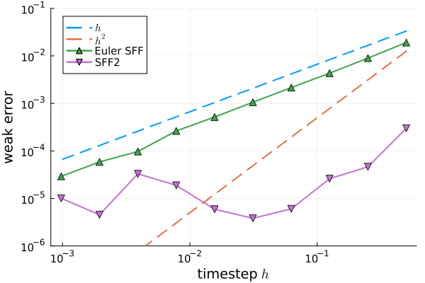
Refer to caption
Refer to caption
Figure 1: Brownian excursion at time T=1T=1 on SO3⁡(ℝ)\operatorname{SO}_{3}(\mathbb{R}) represented by the trajectories of the three columns on the sphere 𝕊2\mathbb{S}^{2} (left) and error curve for the weak approximation of Brownian dynamics on SO3⁡(ℝ)\operatorname{SO}_{3}(\mathbb{R}) with ϕ​(x)=exp⁡(−Tr⁡((x−Id)T​(x−Id))/2​d)\phi(x)=\exp(-\operatorname{Tr}((x-I_{d})^{T}(x-I_{d}))/2d), T=1T=1 and M=108M=10^{8} trajectories (right).

5.3 Ergodic dynamics on the sphere

Our second test case focuses on the sampling of Riemannian Langevin dynamics on the sphere 𝕊2\mathbb{S}^{2}, following the experiment of [10]. While the approximation for the invariant measure is not the focus of the new methods implemented in this paper, this example allows us to conveniently compare the performance of the new frozen flow methods to the alternatives from the literature. The sphere 𝕊d\mathbb{S}^{d} can be seen as a homogeneous manifold with respect to the Lie group G=SOd+1⁡(ℝ)G=\operatorname{SO}_{d+1}(\mathbb{R}), so that we could consider a natural frame derived from a basis of the Lie algebra 𝔰​𝔬d+1\mathfrak{so}_{d+1} (which would typically fit the simulation of a stochastic rigid body). However, we need an orthonormal frame to sample from the Riemannian Langevin dynamics (1.3), so that we use a different choice of frame relying on the standard spherical coordinates. We consider the coordinates on 𝕊2\mathbb{S}^{2} minus the north/south poles:

yθ,φ=(cos⁡(θ)​cos⁡(φ)cos⁡(θ)​sin⁡(φ)sin⁡(θ))∈𝕊2,θ∈]−π2,π2[,φ∈[0,2π[,y_{\theta,\varphi}=\begin{pmatrix}\cos(\theta)\cos(\varphi)\\ \cos(\theta)\sin(\varphi)\\ \sin(\theta)\end{pmatrix}\in\mathbb{S}^{2},\quad\theta\in]-\frac{\pi}{2},\frac{\pi}{2}[,\quad\varphi\in[0,2\pi[,

with the associated orthonormal frame basis:

E1​(yθ,φ)=(−sin⁡(θ)​cos⁡(φ)−sin⁡(θ)​sin⁡(φ)cos⁡(θ)),E2​(yθ,φ)=(−sin⁡(φ)cos⁡(φ)0),E_{1}(y_{\theta,\varphi})=\begin{pmatrix}-\sin(\theta)\cos(\varphi)\\ -\sin(\theta)\sin(\varphi)\\ \cos(\theta)\end{pmatrix},\quad E_{2}(y_{\theta,\varphi})=\begin{pmatrix}-\sin(\varphi)\\ \cos(\varphi)\\ 0\end{pmatrix},

and a second frame associated to the spherical coordinates on 𝕊2\mathbb{S}^{2} minus [±1,0,0][\pm 1,0,0]. Using two frames guarantees a bounded Lipschitz constant for the chosen frame and does not impact the sampled measure. As the manifold is compact, the assumptions of our analysis are satisfied automatically. The frozen flow is computed explicitly in coordinates. In order to obtain a fair comparison between the methods, we use Gaussian random variables.

We now compare the numerical behaviour of the frozen flow Euler method (2.8), the new second order method (2.10), the Riemmanian Langevin method [10], and the extrinsic projection methods of order one [60] for sampling the invariant measure of Riemannian Langevin dynamics (1.3) on 𝕊2\mathbb{S}^{2}. We consider the potential V​(yθ,φ)=−sin⁡(θ)V(y_{\theta,\varphi})=-\sin(\theta), the associated vector field (containing the Ito correction)

F=−∇V−∇E1E1−∇E2E2,F=-\nabla V-\nabla_{E_{1}}E_{1}-\nabla_{E_{2}}E_{2},

and the test function ϕ​(x)=x32\phi(x)=x_{3}^{2}. In this context, the generator is ℒ​ϕ=−ϕ′​(∇V)+12​Δ𝕊2\mathcal{L}\phi=-\phi^{\prime}(\nabla V)+\frac{1}{2}\Delta_{\mathbb{S}^{2}}, with the spherical Laplacian Δ𝕊2\Delta_{\mathbb{S}^{2}}. Assuming ergodicity (which is observed numerically for the methods studied here), the numerical schemes approximate the quantity

∫𝕊2ϕ​(x)​e−V​(x)​d​vol⁡(x)∫𝕊2e−V​(x)​d​vol⁡(x)=3−2tanh⁡(1).\frac{\int_{\mathbb{S}^{2}}\phi(x)e^{-V(x)}d\operatorname{vol}(x)}{\int_{\mathbb{S}^{2}}e^{-V(x)}d\operatorname{vol}(x)}=3-\frac{2}{\tanh(1)}.

We observe the weak error curves in Figure 2, as well as the expected orders of convergence. The new second-order frozen flow method outperforms the other integrators and reaches the Monte-Carlo threshold with much larger timestep.

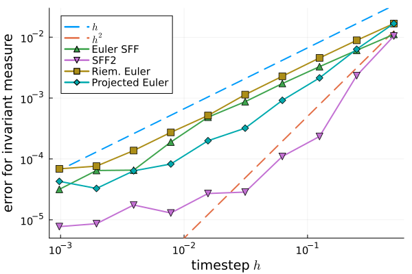
Refer to caption
Refer to caption
Figure 2: A trajectory of the new second order method (2.11) (left) and the convergence curve for the weak approximation of stochastic rigid body equation on the sphere (right) with ϕ​(x)=x32\phi(x)=x_{3}^{2}, T=10T=10 and M=108M=10^{8} trajectories.

5.4 Generalised Cauchy measures

The generalised Cauchy measures are probability measures μβ\mu_{\beta} defined on ℝn\mathbb{R}^{n} by

μβ​(d​x)=(1+|x|2)−β​d​xZβ,Zβ=Γ​(β−n/2)Γ​(β),\mu_{\beta}(dx)=\left(1+|x|^{2}\right)^{-\beta}\frac{dx}{Z_{\beta}},\quad Z_{\beta}=\frac{\Gamma(\beta-n/2)}{\Gamma(\beta)},

with β>n/2\beta>n/2. They can be interpreted as finite dimensional approximations of Gaussian distributions, as in [11], and are related to the fast diffusion equation for which they play the role of the heat kernel and are known as Barenblatt’ solutions (see [90]). A generalised Cauchy measure is the ergodic distribution of the dynamics

d​Xt=−2​(β−1)​Xt​d​t+2​(1+|Xt|2)​d​B​(t),dX_{t}=-2(\beta-1)X_{t}dt+\sqrt{2}(1+|X_{t}|^{2})dB(t), (5.1)

where B​(t)B(t) is a 2-dimensional Brownian motion. A direct numerical simulation of this SDE presents numerous difficulties as the multiplicative non-Lipschitz noise brings tedious stability problems, so that most standard Euclidean numerical methods fail. However, the noise can be interpreted as additive at the cost of a change of metric gx=(1+|x|2)−1​⟨⋅,⋅⟩g_{x}=(1+|x|^{2})^{-1}\langle\cdot,\cdot\rangle. This change is not simply a transport of difficulties from noise to geometry, as it reinterprets the problem in a convenient space. The same approach has been fruitful in the study of the associated spectral gap, i.e. the speed of convergence of the semigroup to the ergodic measure, in [45]. This context calls for methods on manifolds, as Euclidean methods are not adapted. We emphasize that the process (Xt)t(X_{t})_{t} does not have bounded moments at all orders. Thus, the convergence results of the standard Euclidean analysis, and of our analysis as well, do not hold. This makes the simulation of generalised Cauchy measures a convenient toy problem for testing our methods.

We are concerned with the simulation of generalised Cauchy measure on ℝ2\mathbb{R}^{2}. As explained in [44], the adapted manifold can be interpreted as the revolution surface

SS={(tanh⁡(r)​cos⁡(θ),tanh⁡(r)​sin⁡(θ),h​(r));(r,θ)∈ℝ+×𝕊1},\SS=\left\{(\tanh(r)\cos(\theta),\tanh(r)\sin(\theta),h(r));(r,\theta)\in\mathbb{R}_{+}\times\mathbb{S}^{1}\right\}, (5.2)

with h​(r)=argsinh⁡(cosh⁡(r))−cosh−2⁡(r)​cosh2⁡(r)+1h(r)=\operatorname{argsinh}(\cosh(r))-\cosh^{-2}(r)\sqrt{\cosh^{2}(r)+1}. However, it is more handy to see it through a global map, as ℝ+×𝕊1\mathbb{R}_{+}\times\mathbb{S}^{1}, with coordinate (r,θ)(r,\theta), endowed with the metric

g=(100tanh2⁡(r))g=\begin{pmatrix}1&0\\ 0&\tanh^{2}(r)\\ \end{pmatrix}

in the basis (∂r,∂θ)(\partial_{r},\partial_{\theta}). This map comes from fitting polar coordinates on ℝ2\mathbb{R}^{2},

(x,y)=(sinh⁡(r)​cos⁡(θ),sinh⁡(r)​sin⁡(θ)),(x,y)=(\sinh(r)\cos(\theta),\sinh(r)\sin(\theta)),

which trivialise the metric gg. We define the following orthonormal frame basis on ℝ+∗×𝕊1\mathbb{R}^{*}_{+}\times\mathbb{S}^{1}

E1​(r,θ)=∂r,E2​(r,θ)=1tanh⁡(r)​∂θ.E_{1}(r,\theta)=\partial_{r},\quad E_{2}(r,\theta)=\frac{1}{\tanh(r)}\partial_{\theta}.

In this manifold, generalised Cauchy measures correspond to Gibbs measures associated to the potential Vβ​(r,θ)=2​(β−1)​log⁡(cosh⁡(r))V_{\beta}(r,\theta)=2(\beta-1)\log(\cosh(r)) and the generator

ℒ=E12+E22+(1tanh⁡(r)−(2​β−1)​tanh⁡(r))​E1.\mathcal{L}=E_{1}^{2}+E_{2}^{2}+\left(\frac{1}{\tanh(r)}-(2\beta-1)\tanh(r)\right)E_{1}.

Note that the frozen flow is explicit on SS\SS. For all α,β∈ℝ\alpha,\beta\in\mathbb{R} and (r0,θ0)∈ℝ+∗×𝕊1(r_{0},\theta_{0})\in\mathbb{R}_{+}^{*}\times\mathbb{S}^{1}, we find

exp⁡(t​(α​E1+β​E2))⋅(r0,θ0)=(r0+α​t,θ0+βα​log⁡(sinh⁡(r0+α​t)sinh⁡(r0))),\exp\left(t(\alpha E_{1}+\beta E_{2})\right)\cdot(r_{0},\theta_{0})=\left(r_{0}+\alpha t,\theta_{0}+\frac{\beta}{\alpha}\log\left(\frac{\sinh(r_{0}+\alpha t)}{\sinh(r_{0})}\right)\right),

for all t≥0t\geq 0 such that rtr_{t} stays positive. This brings an additional difficulty in this experiment. Although the potential f1f^{1} blows up at the origin, the coefficient

α=h​f1​(r)+2​h​ξ\alpha=hf^{1}(r)+\sqrt{2h}\xi

with ξ\xi a Gaussian random variable, can be negative and the frozen flow not defined. The use of bounded random variable is instrumental in avoiding this instability. In particular, the method (2.8) with Rademacher random variables is well-posed.

Our numerical experiment aims to illustrate the ergodicity of the simplest frozen flow method (2.8), which, to the best of our knowledge, has not yet been established in the literature. We use the first eigenfunctions of the generator ϕ1(r,θ)=sinh(r)2−(β−2)−1\phi^{1}(r,\theta)=\sinh(r)^{2}-(\beta-2)^{-1}, ϕ2​(r,θ)=sinh⁡(r)​cos⁡(θ)\phi^{2}(r,\theta)=\sinh(r)\cos(\theta), which both satisfy ∫ϕk​𝑑μβ=0\int\phi^{k}\,d\mu_{\beta}=0. As a consequence of the Poincaré inequality, the variance of the semigroup associated to ℒ\mathcal{L} converges at exponential speed to 0. The coefficient of the exponential is given by the spectral gap (see [46] for the spectral gap expression). The test functions ϕk\phi^{k} are extremal for the Poincaré inequality. Hence, for these particular test functions, the exponential convergence can be observed not only for the variance but also pointwise. In Figure 3, we illustrate numerically the exponential convergence to equilibrium of the numerical methods, in the spirit of [33] in the Euclidean setting. In particular, we observe a convergence in C​e−4​(β−2)​tCe^{-4(\beta-2)t} and C​e−2​(β−1)​tCe^{-2(\beta-1)t} for our specific choice of test functions, confirming numerically the results in [46]. For the first eigenfunction ϕ1\phi^{1}, the error for the invariant measure reaches the discretisation bias with exponential speed. We observe that the bias threshold evolves linearly in hh (up to Monte-Carlo error), as expected for a method of order one. For ϕ2\phi^{2}, we do not observe the bias of the Euler frozen flow method (2.8), hinting that for this specific test function, the method might be of higher order of accuracy for the invariant measure. For the sake of comparison, we mention that the standard Euclidean integrators applied to (5.1) face severe instability issues and thus fail to converge, let alone be ergodic.

Refer to caption
Refer to caption
Figure 3: Evolution in time of the error for the invariant measure of the Euler frozen flow method (2.8) for the simulation of generalised Cauchy measures on the manifold (5.2) with β=4\beta=4, M=108M=10^{8} trajectories, and the test functions ϕ1(r,θ)=sinh(r)2−(β−2)−1\phi^{1}(r,\theta)=\sinh(r)^{2}-(\beta-2)^{-1} (left) and ϕ2​(r,θ)=sinh⁡(r)​cos⁡(θ)\phi^{2}(r,\theta)=\sinh(r)\cos(\theta) (right).

6 Conclusion

In this paper, we provided a brand-new class of intrinsic discretisations for the approximation of stochastic dynamics on Riemannian manifolds with high weak order of accuracy. We presented a new robust convergence analysis, that naturally generalises the Euclidean analysis, and the new algebraic formalism of planar exotic trees, forests, and series for the study of the order conditions. The analysis applies in particular for the creation of high-order sampling methods for Riemannian Langevin dynamics. The new methods were tested on a variety of different manifolds, where we observe that the new second order frozen flow method outperforms the other approaches from the literature in terms of accuracy.

The tools developed in the present paper open several avenues for future research. Similar to the Euclidean setting, we will extend the analysis to general SDEs with multiplicative noise and to the creation of integrators with high-order of accuracy for sampling the invariant measure, and low weak order (in the spirit of [57, 91]). This requires generalisations of the exotic forests formalism [20], the challenging extension of the integration by parts of trees in the planar case [55, 56, 14, 15], and the extension of stochastic backward error analysis for the invariant measure [86, 93, 33, 2, 15] on manifolds. While the focus of this paper is on discretisations and improvements in accuracy only, our approach could naturally be combined with popular sampling techniques, such as MLMC [38, 39], perturbations [59, 34, 1],… Then, following the work [10], one could wonder whether a purely Riemannian approach of algebraic order theory could be used. Our approach follows the one of deterministic Lie-group methods and thus relies on a curvature-free connection, unrelated to the natural Levi-Civita connection on Riemannian manifolds. The study of such new methods is already open in the deterministic setting and relies on the challenging general understanding of the connection algebra [5]. Finally, the new algebraic formalism of planar exotic series is interesting in itself and could be studied for its universal combinatorial, algebraic, and geometric properties, but also for its potential applications in different fields, in the spirit of the use of Butcher series and their extensions in rough paths [42, 58], renormalisation theory [17], variational calculus [53, 52] or approximation of PDEs [16]. These projects will be studied in upcoming works.


Acknowledgements. The authors would like to thank R. Bergmann, E. Celledoni, H. Munthe-Kaas, and B. Owren for helpful discussions and advice on manipulating the package Manifolds.jl [7]. The authors acknowledge the support of the Swiss National Science Foundation, projects No 200020_214819, and No. 200020_192129, of the Research Council of Norway through project 302831 “Computational Dynamics and Stochastics on Manifolds” (CODYSMA), and of the French program ANR-11-LABX-0020-0 (Labex Lebesgue). The computations were performed on the Baobab cluster of the University of Geneva.

References

  • [1] A. Abdulle, G. A. Pavliotis, and G. Vilmart. Accelerated convergence to equilibrium and reduced asymptotic variance for Langevin dynamics using Stratonovich perturbations. C. R. Math. Acad. Sci. Paris, 357(4):349–354, 2019.
  • [2] A. Abdulle, G. Vilmart, and K. C. Zygalakis. High order numerical approximation of the invariant measure of ergodic SDEs. SIAM J. Numer. Anal., 52(4):1600–1622, 2014.
  • [3] M. Ableidinger and E. Buckwar. Weak stochastic Runge–Kutta Munthe-Kaas methods for finite spin ensembles. Applied Numerical Mathematics, 118:50–63, 2017.
  • [4] P.-A. Absil, R. Mahony, and R. Sepulchre. Optimization algorithms on matrix manifolds. Princeton University Press, Princeton, NJ, 2008. With a foreword by Paul Van Dooren.
  • [5] M. J. H. Al-Kaabi, K. Ebrahimi-Fard, D. Manchon, and H. Z. Munthe-Kaas. Algebraic aspects of connections: from torsion, curvature, and post-lie algebras to Gavrilov’s double exponential and special polynomials. Submitted, 2022.
  • [6] A. Antonyuk and A. Antonyuk. Nonexplosion and solvability of nonlinear diffusion equations on noncompact manifolds. Ukr. Math. J., 59:1632–1652, 2007.
  • [7] S. D. Axen, M. Baran, R. Bergmann, and K. Rzecki. Manifolds.jl: An extensible julia framework for data analysis on manifolds. ACM Transactions on Mathematical Software, 49(4), dec 2023.
  • [8] D. Bakry. Un critère de non-explosion pour certaines diffusions sur une variété riemannienne complète. C.R. Acad. Sc. Paris, 303(1):23–26, 1986.
  • [9] D. Bakry, I. Gentil, and M. Ledoux. Analysis and geometry of Markov diffusion operators, volume 348 of Grundlehren Math. Wiss. Cham: Springer, 2014.
  • [10] K. Bharath, A. Lewis, A. Sharma, and M. V. Tretyakov. Sampling and estimation on manifolds using the Langevin diffusion. arXiv:2312.14882, 2023.
  • [11] S. G. Bobkov and M. Ledoux. Weighted Poincaré-type inequalities for Cauchy and other convex measures. Ann. Probab., 37(2):403–427, 2009.
  • [12] G. Bogfjellmo. Algebraic structure of aromatic B-series. J. Comput. Dyn., 6(2):199–222, 2019.
  • [13] G. Bogfjellmo, E. Celledoni, R. I. McLachlan, B. Owren, and G. R. W. Quispel. Using aromas to search for preserved measures and integrals in Kahan’s method. Math. Comp., 93(348):1633–1653, 2024.
  • [14] E. Bronasco. Exotic B-series and S-series: algebraic structures and order conditions for invariant measure sampling. Found. Comput. Math., pages 1–31, 2024.
  • [15] E. Bronasco and A. Laurent. Hopf algebra structures for the backward error analysis of ergodic stochastic differential equations. arXiv:2407.07451, 2024.
  • [16] Y. A. Bronsard, Y. Bruned, and K. Schratz. Approximations of dispersive PDEs in the presence of low-regularity randomness. arXiv preprint arXiv:2205.02156, 2022.
  • [17] C. Brouder. Runge–Kutta methods and renormalization. Eur. Phys. J. C, 12(3):521–534, 2000.
  • [18] K. Burrage and P. M. Burrage. High strong order methods for non-commutative stochastic ordinary differential equation systems and the Magnus formula. Phys. D, 133(1-4):34–48, 1999. Predictability: quantifying uncertainty in models of complex phenomena (Los Alamos, NM, 1998).
  • [19] P. M. Burrage. Runge-Kutta methods for stochastic differential equations. PhD thesis, Dept. Maths., Univ. Queensland, Australia, 1999.
  • [20] A. Busnot Laurent, K. Debrabant, and A. Kværnø. Optimal stochastic Runge-Kutta methods for the weak integration of stochastic dynamics. Preprint, 2025.
  • [21] J. C. Butcher. Numerical methods for ordinary differential equations. John Wiley & Sons, Ltd., Chichester, third edition, 2016.
  • [22] J. C. Butcher. B-series: algebraic analysis of numerical methods. Springer, 2021.
  • [23] D. Calaque, K. Ebrahimi-Fard, and D. Manchon. Two interacting Hopf algebras of trees: a Hopf-algebraic approach to composition and substitution of B-series. Adv. in Appl. Math., 47(2):282–308, 2011.
  • [24] P. Catoire. The Cartier-Quillen-Milnor-Moore theorem in the Post-Hopf case. arXiv preprint arXiv:2401.09116, 2024.
  • [25] E. Celledoni, A. Marthinsen, and B. Owren. Commutator-free Lie group methods. Future Generation Computer Systems, 19(3):341–352, 2003.
  • [26] P. Chartier, E. Hairer, and G. Vilmart. Algebraic structures of B-series. Found. Comput. Math., 10(4):407–427, 2010.
  • [27] P. Chartier and A. Murua. Preserving first integrals and volume forms of additively split systems. IMA J. Numer. Anal., 27(2):381–405, 2007.
  • [28] X. Cheng, J. Zhang, and S. Sra. Efficient sampling on Riemannian manifolds via Langevin MCMC. Advances in Neural Information Processing Systems, 35:5995–6006, 2022.
  • [29] P. E. Crouch and R. Grossman. Numerical integration of ordinary differential equations on manifolds. Journal of Nonlinear Science, 3:1–33, 1993.
  • [30] C. Curry and A. Schmeding. Convergence of lie group integrators. Numerische Mathematik, 144:357–373, 2020.
  • [31] R. L. Davidchack, T. Ouldridge, and M. Tretyakov. New Langevin and gradient thermostats for rigid body dynamics. The Journal of chemical physics, 142(14), 2015.
  • [32] K. Debrabant. Runge-Kutta methods for third order weak approximation of SDEs with multidimensional additive noise. BIT Numer. Math., 50(3):541–558, 2010.
  • [33] A. Debussche and E. Faou. Weak backward error analysis for SDEs. SIAM J. Numer. Anal., 50(3):1735–1752, 2012.
  • [34] A. B. Duncan, T. Lelièvre, and G. A. Pavliotis. Variance reduction using nonreversible Langevin samplers. J. Stat. Phys., 163(3):457–491, 2016.
  • [35] K. Ebrahimi-Fard, A. Lundervold, and H. Z. Munthe-Kaas. On the Lie enveloping algebra of a post-Lie algebra. J. Lie Theory, 25(4):1139–1165, 2015.
  • [36] K. Ebrahimi-Fard and L. Rahm. A survey on the Munthe-Kaas–Wright Hopf algebra. Journal of Computational Dynamics, 2024.
  • [37] K. Engø, A. Marthinsen, and H. Z. Munthe-Kaas. Diffman: An object-oriented matlab toolbox for solving differential equations on manifolds. Applied numerical mathematics, 39(3-4):323–347, 2001.
  • [38] M. B. Giles. Multilevel Monte Carlo path simulation. Oper. Res., 56(3):607–617, 2008.
  • [39] M. B. Giles. Multilevel Monte Carlo methods. Acta Numer., 24:259–328, 2015.
  • [40] E. Grong, H. Z. Munthe-Kaas, and J. Stava. Post-Lie algebra structure of manifolds with constant curvature and torsion. arXiv preprint arXiv:2305.02688, 2023.
  • [41] E. Hairer, C. Lubich, and G. Wanner. Geometric numerical integration, volume 31 of Springer Series in Computational Mathematics. Springer-Verlag, Berlin, second edition, 2006. Structure-preserving algorithms for ordinary differential equations.
  • [42] M. Hairer and D. Kelly. Geometric versus non-geometric rough paths. Ann. Inst. Henri Poincaré Probab. Stat., 51(1):207–251, 2015.
  • [43] E. P. Hsu. Stochastic analysis on manifolds, volume 38 of Graduate Studies in Mathematics. American Mathematical Society, Providence, RI, 2002.
  • [44] B. Huguet. Stochastic calculus on manifold and application to functional inequalities. PhD thesis, Université de Bordeaux, 2020.
  • [45] B. Huguet. Intertwining relations for diffusions in manifolds and applications to functional inequalities. Stoch. Proc. and their App., 145:1–28, 2022.
  • [46] B. Huguet. Poincaré inequalities and integrated curvature-dimension criterion for generalised cauchy and convex measures. Bernoulli, 30(3):2207–2227, 2024.
  • [47] A. Iserles, H. Z. Munthe-Kaas, S. P. Nørsett, and A. Zanna. Lie-group methods. In Acta numerica, 2000, volume 9 of Acta Numer., pages 215–365. Cambridge Univ. Press, Cambridge, 2000.
  • [48] A. Iserles, G. R. W. Quispel, and P. S. P. Tse. B-series methods cannot be volume-preserving. BIT Numer. Math., 47(2):351–378, 2007.
  • [49] L. Isserlis. On a formula for the product-moment coefficient of any order of a normal frequency distribution in any number of variables. Biometrika, 12, 11 1918.
  • [50] K. Kamm, S. Pagliarani, and A. Pascucci. On the stochastic Magnus expansion and its application to SPDEs. J. Sci. Comput., 89(3):Paper No. 56, 31, 2021.
  • [51] A. Laurent. Algebraic Tools and Multiscale Methods for the Numerical Integration of Stochastic Evolutionary Problems. PhD thesis, University of Geneva, 2021.
  • [52] A. Laurent. The Lie derivative and Noether’s theorem on the aromatic bicomplex for the study of volume-preserving numerical integrators. J. Comput. Dyn., 11(1):10–22, 2024.
  • [53] A. Laurent, R. I. McLachlan, H. Z. Munthe-Kaas, and O. Verdier. The aromatic bicomplex for the description of divergence-free aromatic forms and volume-preserving integrators. Forum Math. Sigma, 11:Paper No. e69, 2023.
  • [54] A. Laurent and H. Z. Munthe-Kaas. The universal equivariance properties of exotic aromatic B-series. Foundations of Computational Mathematics, pages 1–32, 2024.
  • [55] A. Laurent and G. Vilmart. Exotic aromatic B-series for the study of long time integrators for a class of ergodic SDEs. Math. Comp., 89(321):169–202, 2020.
  • [56] A. Laurent and G. Vilmart. Order conditions for sampling the invariant measure of ergodic stochastic differential equations on manifolds. Found. Comput. Math., 22(3):649–695, 2022.
  • [57] B. Leimkuhler and C. Matthews. Rational construction of stochastic numerical methods for molecular sampling. Appl. Math. Res. Express. AMRX, 2013(1):34–56, 2013.
  • [58] A. Lejay. Constructing general rough differential equations through flow approximations. Electron. J. Probab., 27:Paper No. 7, 24, 2022.
  • [59] T. Lelièvre, F. Nier, and G. A. Pavliotis. Optimal non-reversible linear drift for the convergence to equilibrium of a diffusion. J. Stat. Phys., 152(2):237–274, 2013.
  • [60] T. Lelièvre, M. Rousset, and G. Stoltz. Free energy computations. Imperial College Press, London, 2010. A mathematical perspective.
  • [61] X.-M. Li. Stochastic differential equations on noncompact manifolds: moment stability and its topological consequences. Probab. Theory Relat. Fields, 100:417–428, 1994.
  • [62] Y. Li, Y. Sheng, and R. Tang. Post-hopf algebras, relative rota–baxter operators and solutions to the yang–baxter equation. Journal of Noncommutative Geometry, 18(2):605–630, 2023.
  • [63] A. Lundervold and H. Munthe-Kaas. Hopf algebras of formal diffeomorphisms and numerical integration on manifolds. In Combinatorics and physics, volume 539 of Contemp. Math., pages 295–324. Amer. Math. Soc., Providence, RI, 2011.
  • [64] S. J. A. Malham and A. Wiese. Stochastic Lie group integrators. SIAM J. Sci. Comput., 30(2):597–617, 2008.
  • [65] G. Marjanovic, M. J. Piggott, and V. Solo. A simple approach to numerical methods for stochastic differential equations in Lie groups. In 2015 54th IEEE Conference on Decision and Control (CDC), pages 7143–7150. IEEE, 2015.
  • [66] G. Marjanovic and V. Solo. Numerical methods for stochastic differential equations in matrix Lie groups made simple. IEEE Trans. Automat. Control, 63(12):4035–4050, 2018.
  • [67] R. I. McLachlan, K. Modin, H. Munthe-Kaas, and O. Verdier. B-series methods are exactly the affine equivariant methods. Numer. Math., 133(3):599–622, 2016.
  • [68] R. I. McLachlan, K. Modin, H. Munthe-Kaas, and O. Verdier. Butcher series: a story of rooted trees and numerical methods for evolution equations. Asia Pac. Math. Newsl., 7(1):1–11, 2017.
  • [69] G. N. Milstein and M. V. Tretyakov. Stochastic numerics for mathematical physics. Scientific Computation. Springer-Verlag, Berlin, 2004.
  • [70] H. Munthe-Kaas. Lie-Butcher theory for Runge-Kutta methods. BIT Numer. Math., 35:572–587, 1995.
  • [71] H. Munthe-Kaas. Runge-Kutta methods on Lie groups. BIT Numer. Math., 38:92–111, 1998.
  • [72] H. Munthe-Kaas. High order Runge-Kutta methods on manifolds. Applied Numerical Mathematics, 29(1):115–127, 1999.
  • [73] H. Munthe-Kaas. Geometric integration on symmetric spaces. J. Comput. Dyn., 11(1):43–58, 2024.
  • [74] H. Munthe-Kaas and J. Stava. Lie admissible triple algebras: The connection algebra of symmetric spaces. Submitted, 2023.
  • [75] H. Munthe-Kaas and O. Verdier. Aromatic Butcher series. Found. Comput. Math., 16(1):183–215, 2016.
  • [76] H. Munthe-Kaas and O. Verdier. Integrators on homogeneous spaces: Isotropy choice and connections. Foundations of Computational Mathematics, 16:899–939, 2016.
  • [77] H. Munthe-Kaas and A. Zanna. Numerical integration of differential equations on homogeneous manifolds. In Foundations of Computational Mathematics: Selected Papers of a Conference Held at Rio de Janeiro, January 1997, pages 305–315. Springer, 1997.
  • [78] H. Z. Munthe-Kaas and A. Lundervold. On post-Lie algebras, Lie–Butcher series and moving frames. Foundations of Computational Mathematics, 13:583–613, 2013.
  • [79] H. Z. Munthe-Kaas and W. M. Wright. On the Hopf algebraic structure of Lie group integrators. Found. Comput. Math., 8(2):227–257, 2008.
  • [80] J.-M. Oudom and D. Guin. On the Lie enveloping algebra of a pre-Lie algebra. J. K-Theory, 2(1):147–167, 2008.
  • [81] B. Owren. Order conditions for commutator-free Lie group methods. Journal of Physics A: Mathematical and General, 39(19):5585, 2006.
  • [82] B. Owren and A. Marthinsen. Runge-Kutta methods adapted to manifolds and based on rigid frames. BIT Numer. Math., 39(1):116–142, 1999.
  • [83] L. Rahm. An operadic approach to substitution in Lie-Butcher series. Forum Math. Sigma, 10:Paper No. e20, 29, 2022.
  • [84] A. Rößler. Runge-Kutta methods for Stratonovich stochastic differential equation systems with commutative noise. In Proceedings of the 10th International Congress on Computational and Applied Mathematics (ICCAM-2002), volume 164/165, pages 613–627, 2004.
  • [85] A. Rößler. Stochastic Taylor expansions for the expectation of functionals of diffusion processes. Stochastic Anal. Appl., 22(6):1553–1576, 2004.
  • [86] T. Shardlow. Modified equations for stochastic differential equations. BIT Numer. Math., 46(1):111–125, 2006.
  • [87] D. Talay. Second-order discretization schemes of stochastic differential systems for the computation of the invariant law. Stochastics: An International Journal of Probability and Stochastic Processes, 29(1):13–36, 1990.
  • [88] D. Talay and L. Tubaro. Expansion of the global error for numerical schemes solving stochastic differential equations. Stochastic Anal. Appl., 8(4):483–509 (1991), 1990.
  • [89] J. Thompson. Brownian motion and the distance to a submanifold. Potential Anal., 45(3):485–508, 2016.
  • [90] J. L. Vázquez. The porous medium equation. Mathematical theory. Oxford Math. Monogr. Oxford: Oxford University Press, 2007.
  • [91] G. Vilmart. Postprocessed integrators for the high order integration of ergodic SDEs. SIAM J. Sci. Comput., 37(1):A201–A220, 2015.
  • [92] Z. Wang, Q. Ma, Z. Yao, and X. Ding. The Magnus expansion for stochastic differential equations. J. Nonlinear Sci., 30(1):419–447, 2020.
  • [93] K. C. Zygalakis. On the existence and the applications of modified equations for stochastic differential equations. SIAM J. Sci. Comput., 33(1):102–130, 2011.

Appendix A Order conditions for third weak order

For the sake of completion, we detail in Table LABEL:table:weak_order_conditions_order_3 the 92 additional order conditions for weak order 3 with stochastic frozen flow methods (2.7). Recall that these conditions are not independent and satisfy shuffle relations (see Remark 2.14), so that only 70 of these conditions are actually necessary.

Table 2: Order conditions of frozen flow methods for weak order 3. The expectations and sums that do not satisfy inequalities are omitted for conciseness.
Exotic forest ​π\text{Exotic forest }\pi a​(π)a(\pi) e​(π)e(\pi)
\forest​b​[b​[b]]\forest{b[b[b]]} zi,k30​Zi,j,k20​Zj,k,k10z^{0}_{i,k_{3}}Z^{0}_{i,j,k_{2}}Z^{0}_{j,k,k_{1}} 16\frac{1}{6}
\forest​b​[b,b]\forest{b[b,b]} ∑k1≥k2!zi,k30​Zi,j,k20​Zi,k,k10\sum^{!}_{k_{1}\geq k_{2}}z^{0}_{i,k_{3}}Z^{0}_{i,j,k_{2}}Z^{0}_{i,k,k_{1}} 16\frac{1}{6}
\forest​b​[b​[1,1]]\forest{b[b[1,1]]} ∑k1≥k2!zi,k40​Zi,j,k30​Zj,k2d1​Zj,k1d1\sum^{!}_{k_{1}\geq k_{2}}z^{0}_{i,k_{4}}Z^{0}_{i,j,k_{3}}Z^{d_{1}}_{j,k_{2}}Z^{d_{1}}_{j,k_{1}} 16\frac{1}{6}
\forest​b​[b​[1],1]\forest{b[b[1],1]} ∑k1≥k3!zi,k40​Zi,j,k30​Zj,k2d1​Zi,k1d1\sum^{!}_{k_{1}\geq k_{3}}z^{0}_{i,k_{4}}Z^{0}_{i,j,k_{3}}Z^{d_{1}}_{j,k_{2}}Z^{d_{1}}_{i,k_{1}} 13\frac{1}{3}
\forest​b​[1,b​[1]]\forest{b[1,b[1]]} ∑k3≥k1!zi,k40​Zi,j,k30​Zj,k2d1​Zi,k1d1\sum^{!}_{k_{3}\geq k_{1}}z^{0}_{i,k_{4}}Z^{0}_{i,j,k_{3}}Z^{d_{1}}_{j,k_{2}}Z^{d_{1}}_{i,k_{1}} 13\frac{1}{3}
\forest​b​[b,1,1]\forest{b[b,1,1]} ∑k1≥k2≥k3!zi,k40​Zi,j,k30​Zi,k2d1​Zi,k1d1\sum^{!}_{k_{1}\geq k_{2}\geq k_{3}}z^{0}_{i,k_{4}}Z^{0}_{i,j,k_{3}}Z^{d_{1}}_{i,k_{2}}Z^{d_{1}}_{i,k_{1}} 16\frac{1}{6}
\forest​b​[1,b,1]\forest{b[1,b,1]} ∑k1≥k3≥k2!zi,k40​Zi,j,k30​Zi,k2d1​Zi,k1d1\sum^{!}_{k_{1}\geq k_{3}\geq k_{2}}z^{0}_{i,k_{4}}Z^{0}_{i,j,k_{3}}Z^{d_{1}}_{i,k_{2}}Z^{d_{1}}_{i,k_{1}} 0
\forest​b​[1,1,b]\forest{b[1,1,b]} ∑k3≥k1≥k2!zi,k40​Zi,j,k30​Zi,k2d1​Zi,k1d1\sum^{!}_{k_{3}\geq k_{1}\geq k_{2}}z^{0}_{i,k_{4}}Z^{0}_{i,j,k_{3}}Z^{d_{1}}_{i,k_{2}}Z^{d_{1}}_{i,k_{1}} 16\frac{1}{6}
\forest​b​[2,2,1,1]\forest{b[2,2,1,1]} ∑k1≥k2≥k3≥k4!zi,k50​Zi,k4d2​Zi,k3d2​Zi,k2d1​Zi,k1d1\sum^{!}_{k_{1}\geq k_{2}\geq k_{3}\geq k_{4}}z^{0}_{i,k_{5}}Z^{d_{2}}_{i,k_{4}}Z^{d_{2}}_{i,k_{3}}Z^{d_{1}}_{i,k_{2}}Z^{d_{1}}_{i,k_{1}} 16\frac{1}{6}
\forest​b​[2,1,2,1]\forest{b[2,1,2,1]} ∑k1≥k2≥k3≥k4!zi,k50​Zi,k4d2​Zi,k3d1​Zi,k2d2​Zi,k1d1\sum^{!}_{k_{1}\geq k_{2}\geq k_{3}\geq k_{4}}z^{0}_{i,k_{5}}Z^{d_{2}}_{i,k_{4}}Z^{d_{1}}_{i,k_{3}}Z^{d_{2}}_{i,k_{2}}Z^{d_{1}}_{i,k_{1}} 0
\forest​b​[1,2,2,1]\forest{b[1,2,2,1]} ∑k1≥k2≥k3≥k4!zi,k50​Zi,k4d1​Zi,k3d2​Zi,k2d2​Zi,k1d1\sum^{!}_{k_{1}\geq k_{2}\geq k_{3}\geq k_{4}}z^{0}_{i,k_{5}}Z^{d_{1}}_{i,k_{4}}Z^{d_{2}}_{i,k_{3}}Z^{d_{2}}_{i,k_{2}}Z^{d_{1}}_{i,k_{1}} 0
\forest​b​[b],b\forest{b[b],b} ∑k1≥k2!Zj,k,k30​zj,k20​zi,k10\sum^{!}_{k_{1}\geq k_{2}}Z^{0}_{j,k,k_{3}}z^{0}_{j,k_{2}}z^{0}_{i,k_{1}} 16\frac{1}{6}
\forest​b,b​[b]\forest{b,b[b]} ∑k2≥k1!Zj,k,k30​zj,k20​zi,k10\sum^{!}_{k_{2}\geq k_{1}}Z^{0}_{j,k,k_{3}}z^{0}_{j,k_{2}}z^{0}_{i,k_{1}} 13\frac{1}{3}
\forest​b​[1,1],b\forest{b[1,1],b} ∑k1≥k2,k3≥k4!Zj,k4d1​Zj,k3d1​zj,k20​zi,k10\sum^{!}_{k_{1}\geq k_{2},k_{3}\geq k_{4}}Z^{d_{1}}_{j,k_{4}}Z^{d_{1}}_{j,k_{3}}z^{0}_{j,k_{2}}z^{0}_{i,k_{1}} 16\frac{1}{6}
\forest​b,b​[1,1]\forest{b,b[1,1]} ∑k2≥k1,k3≥k4!Zj,k4d1​Zj,k3d1​zj,k20​zi,k10\sum^{!}_{k_{2}\geq k_{1},k_{3}\geq k_{4}}Z^{d_{1}}_{j,k_{4}}Z^{d_{1}}_{j,k_{3}}z^{0}_{j,k_{2}}z^{0}_{i,k_{1}} 13\frac{1}{3}
\forest​b​[1],b​[1]\forest{b[1],b[1]} ∑k1≥k2!Zj,k4d1​Zi,k3d1​zj,k20​zi,k10\sum^{!}_{k_{1}\geq k_{2}}Z^{d_{1}}_{j,k_{4}}Z^{d_{1}}_{i,k_{3}}z^{0}_{j,k_{2}}z^{0}_{i,k_{1}} 16\frac{1}{6}
\forest​b​[b​[1]],1\forest{b[b[1]],1} ∑k1≥k2!Zj,k4d1​Zi,j,k30​zi,k20​zk1d1\sum^{!}_{k_{1}\geq k_{2}}Z^{d_{1}}_{j,k_{4}}Z^{0}_{i,j,k_{3}}z^{0}_{i,k_{2}}z^{d_{1}}_{k_{1}} 0
\forest​1,b​[b​[1]]\forest{1,b[b[1]]} ∑k2≥k1!Zj,k4d1​Zi,j,k30​zi,k20​zk1d1\sum^{!}_{k_{2}\geq k_{1}}Z^{d_{1}}_{j,k_{4}}Z^{0}_{i,j,k_{3}}z^{0}_{i,k_{2}}z^{d_{1}}_{k_{1}} 13\frac{1}{3}
\forest​b​[b,1],1\forest{b[b,1],1} ∑k1≥k2,k3≥k4!Zi,j,k40​Zi,k3d1​zi,k20​zk1d1\sum^{!}_{k_{1}\geq k_{2},k_{3}\geq k_{4}}Z^{0}_{i,j,k_{4}}Z^{d_{1}}_{i,k_{3}}z^{0}_{i,k_{2}}z^{d_{1}}_{k_{1}} 0
\forest​b​[1,b],1\forest{b[1,b],1} ∑k1≥k2,k4≥k3!Zi,j,k40​Zi,k3d1​zi,k20​zk1d1\sum^{!}_{k_{1}\geq k_{2},k_{4}\geq k_{3}}Z^{0}_{i,j,k_{4}}Z^{d_{1}}_{i,k_{3}}z^{0}_{i,k_{2}}z^{d_{1}}_{k_{1}} 0
\forest​1,b​[b,1]\forest{1,b[b,1]} ∑k2≥k1,k3≥k4!Zi,j,k40​Zi,k3d1​zi,k20​zk1d1\sum^{!}_{k_{2}\geq k_{1},k_{3}\geq k_{4}}Z^{0}_{i,j,k_{4}}Z^{d_{1}}_{i,k_{3}}z^{0}_{i,k_{2}}z^{d_{1}}_{k_{1}} 0
\forest​1,b​[1,b]\forest{1,b[1,b]} ∑k2≥k1,k4≥k3!Zi,j,k40​Zi,k3d1​zi,k20​zk1d1\sum^{!}_{k_{2}\geq k_{1},k_{4}\geq k_{3}}Z^{0}_{i,j,k_{4}}Z^{d_{1}}_{i,k_{3}}z^{0}_{i,k_{2}}z^{d_{1}}_{k_{1}} 13\frac{1}{3}
\forest​b​[2,2,1],1\forest{b[2,2,1],1} ∑k1≥k2,k3≥k4≥k5!Zi,k5d2​Zi,k4d2​Zi,k3d1​zi,k20​zk1d1\sum^{!}_{k_{1}\geq k_{2},k_{3}\geq k_{4}\geq k_{5}}Z^{d_{2}}_{i,k_{5}}Z^{d_{2}}_{i,k_{4}}Z^{d_{1}}_{i,k_{3}}z^{0}_{i,k_{2}}z^{d_{1}}_{k_{1}} 0
\forest​b​[2,1,2],1\forest{b[2,1,2],1} ∑k1≥k2,k3≥k4≥k5!Zi,k5d2​Zi,k4d1​Zi,k3d2​zi,k20​zk1d1\sum^{!}_{k_{1}\geq k_{2},k_{3}\geq k_{4}\geq k_{5}}Z^{d_{2}}_{i,k_{5}}Z^{d_{1}}_{i,k_{4}}Z^{d_{2}}_{i,k_{3}}z^{0}_{i,k_{2}}z^{d_{1}}_{k_{1}} 0
\forest​b​[1,2,2],1\forest{b[1,2,2],1} ∑k1≥k2,k3≥k4≥k5!Zi,k5d1​Zi,k4d2​Zi,k3d2​zi,k20​zk1d1\sum^{!}_{k_{1}\geq k_{2},k_{3}\geq k_{4}\geq k_{5}}Z^{d_{1}}_{i,k_{5}}Z^{d_{2}}_{i,k_{4}}Z^{d_{2}}_{i,k_{3}}z^{0}_{i,k_{2}}z^{d_{1}}_{k_{1}} 0
\forest​1,b​[2,2,1]\forest{1,b[2,2,1]} ∑k2≥k1,k3≥k4≥k5!Zi,k5d2​Zi,k4d2​Zi,k3d1​zi,k20​zk1d1\sum^{!}_{k_{2}\geq k_{1},k_{3}\geq k_{4}\geq k_{5}}Z^{d_{2}}_{i,k_{5}}Z^{d_{2}}_{i,k_{4}}Z^{d_{1}}_{i,k_{3}}z^{0}_{i,k_{2}}z^{d_{1}}_{k_{1}} 13\frac{1}{3}
\forest​1,b​[2,1,2]\forest{1,b[2,1,2]} ∑k2≥k1,k3≥k4≥k5!Zi,k5d2​Zi,k4d1​Zi,k3d2​zi,k20​zk1d1\sum^{!}_{k_{2}\geq k_{1},k_{3}\geq k_{4}\geq k_{5}}Z^{d_{2}}_{i,k_{5}}Z^{d_{1}}_{i,k_{4}}Z^{d_{2}}_{i,k_{3}}z^{0}_{i,k_{2}}z^{d_{1}}_{k_{1}} 0
\forest​1,b​[1,2,2]\forest{1,b[1,2,2]} ∑k2≥k1,k3≥k4≥k5!Zi,k5d1​Zi,k4d2​Zi,k3d2​zi,k20​zk1d1\sum^{!}_{k_{2}\geq k_{1},k_{3}\geq k_{4}\geq k_{5}}Z^{d_{1}}_{i,k_{5}}Z^{d_{2}}_{i,k_{4}}Z^{d_{2}}_{i,k_{3}}z^{0}_{i,k_{2}}z^{d_{1}}_{k_{1}} 13\frac{1}{3}
\forest​b,b,b\forest{b,b,b} ∑k1≥k2≥k3!zk,k30​zj,k20​zi,k10\sum^{!}_{k_{1}\geq k_{2}\geq k_{3}}z^{0}_{k,k_{3}}z^{0}_{j,k_{2}}z^{0}_{i,k_{1}} 16\frac{1}{6}
\forest​b​[1],b,1\forest{b[1],b,1} ∑k1≥k2≥k3!Zj,k4d1​zj,k30​zi,k20​zk1d1\sum^{!}_{k_{1}\geq k_{2}\geq k_{3}}Z^{d_{1}}_{j,k_{4}}z^{0}_{j,k_{3}}z^{0}_{i,k_{2}}z^{d_{1}}_{k_{1}} 0
\forest​b​[1],1,b\forest{b[1],1,b} ∑k2≥k1≥k3!Zj,k4d1​zj,k30​zi,k20​zk1d1\sum^{!}_{k_{2}\geq k_{1}\geq k_{3}}Z^{d_{1}}_{j,k_{4}}z^{0}_{j,k_{3}}z^{0}_{i,k_{2}}z^{d_{1}}_{k_{1}} 0
\forest​b,b​[1],1\forest{b,b[1],1} ∑k1≥k3≥k2!Zj,k4d1​zj,k30​zi,k20​zk1d1\sum^{!}_{k_{1}\geq k_{3}\geq k_{2}}Z^{d_{1}}_{j,k_{4}}z^{0}_{j,k_{3}}z^{0}_{i,k_{2}}z^{d_{1}}_{k_{1}} 0
\forest​b,1,b​[1]\forest{b,1,b[1]} ∑k3≥k1≥k2!Zj,k4d1​zj,k30​zi,k20​zk1d1\sum^{!}_{k_{3}\geq k_{1}\geq k_{2}}Z^{d_{1}}_{j,k_{4}}z^{0}_{j,k_{3}}z^{0}_{i,k_{2}}z^{d_{1}}_{k_{1}} 13\frac{1}{3}
\forest​1,b​[1],b\forest{1,b[1],b} ∑k2≥k3≥k1!Zj,k4d1​zj,k30​zi,k20​zk1d1\sum^{!}_{k_{2}\geq k_{3}\geq k_{1}}Z^{d_{1}}_{j,k_{4}}z^{0}_{j,k_{3}}z^{0}_{i,k_{2}}z^{d_{1}}_{k_{1}} 13\frac{1}{3}
\forest​1,b,b​[1]\forest{1,b,b[1]} ∑k3≥k2≥k1!Zj,k4d1​zj,k30​zi,k20​zk1d1\sum^{!}_{k_{3}\geq k_{2}\geq k_{1}}Z^{d_{1}}_{j,k_{4}}z^{0}_{j,k_{3}}z^{0}_{i,k_{2}}z^{d_{1}}_{k_{1}} 13\frac{1}{3}
\forest​b​[2,2],1,1\forest{b[2,2],1,1} ∑k1≥k2≥k3,k4≥k5!Zi,k5d2​Zi,k4d2​zi,k30​zk2d1​zk1d1\sum^{!}_{k_{1}\geq k_{2}\geq k_{3},k_{4}\geq k_{5}}Z^{d_{2}}_{i,k_{5}}Z^{d_{2}}_{i,k_{4}}z^{0}_{i,k_{3}}z^{d_{1}}_{k_{2}}z^{d_{1}}_{k_{1}} 16\frac{1}{6}
\forest​1,b​[2,2],1\forest{1,b[2,2],1} ∑k1≥k3≥k2,k4≥k5!Zi,k5d2​Zi,k4d2​zi,k30​zk2d1​zk1d1\sum^{!}_{k_{1}\geq k_{3}\geq k_{2},k_{4}\geq k_{5}}Z^{d_{2}}_{i,k_{5}}Z^{d_{2}}_{i,k_{4}}z^{0}_{i,k_{3}}z^{d_{1}}_{k_{2}}z^{d_{1}}_{k_{1}} 0
\forest​1,1,b​[2,2]\forest{1,1,b[2,2]} ∑k3≥k1≥k2,k4≥k5!Zi,k5d2​Zi,k4d2​zi,k30​zk2d1​zk1d1\sum^{!}_{k_{3}\geq k_{1}\geq k_{2},k_{4}\geq k_{5}}Z^{d_{2}}_{i,k_{5}}Z^{d_{2}}_{i,k_{4}}z^{0}_{i,k_{3}}z^{d_{1}}_{k_{2}}z^{d_{1}}_{k_{1}} 13\frac{1}{3}
\forest​b​[2,1],2,1\forest{b[2,1],2,1} ∑k1≥k2≥k3,k4≥k5!Zi,k5d2​Zi,k4d1​zi,k30​zk2d2​zk1d1\sum^{!}_{k_{1}\geq k_{2}\geq k_{3},k_{4}\geq k_{5}}Z^{d_{2}}_{i,k_{5}}Z^{d_{1}}_{i,k_{4}}z^{0}_{i,k_{3}}z^{d_{2}}_{k_{2}}z^{d_{1}}_{k_{1}} 0
\forest​b​[1,2],2,1\forest{b[1,2],2,1} ∑k1≥k2≥k3,k4≥k5!Zi,k5d1​Zi,k4d2​zi,k30​zk2d2​zk1d1\sum^{!}_{k_{1}\geq k_{2}\geq k_{3},k_{4}\geq k_{5}}Z^{d_{1}}_{i,k_{5}}Z^{d_{2}}_{i,k_{4}}z^{0}_{i,k_{3}}z^{d_{2}}_{k_{2}}z^{d_{1}}_{k_{1}} 0
\forest​2,b​[2,1],1\forest{2,b[2,1],1} ∑k1≥k3≥k2,k4≥k5!Zi,k5d2​Zi,k4d1​zi,k30​zk2d2​zk1d1\sum^{!}_{k_{1}\geq k_{3}\geq k_{2},k_{4}\geq k_{5}}Z^{d_{2}}_{i,k_{5}}Z^{d_{1}}_{i,k_{4}}z^{0}_{i,k_{3}}z^{d_{2}}_{k_{2}}z^{d_{1}}_{k_{1}} 0
\forest​2,b​[1,2],1\forest{2,b[1,2],1} ∑k1≥k3≥k2,k4≥k5!Zi,k5d1​Zi,k4d2​zi,k30​zk2d2​zk1d1\sum^{!}_{k_{1}\geq k_{3}\geq k_{2},k_{4}\geq k_{5}}Z^{d_{1}}_{i,k_{5}}Z^{d_{2}}_{i,k_{4}}z^{0}_{i,k_{3}}z^{d_{2}}_{k_{2}}z^{d_{1}}_{k_{1}} 0
\forest​2,1,b​[2,1]\forest{2,1,b[2,1]} ∑k3≥k1≥k2,k4≥k5!Zi,k5d2​Zi,k4d1​zi,k30​zk2d2​zk1d1\sum^{!}_{k_{3}\geq k_{1}\geq k_{2},k_{4}\geq k_{5}}Z^{d_{2}}_{i,k_{5}}Z^{d_{1}}_{i,k_{4}}z^{0}_{i,k_{3}}z^{d_{2}}_{k_{2}}z^{d_{1}}_{k_{1}} 23\frac{2}{3}
\forest​2,1,b​[1,2]\forest{2,1,b[1,2]} ∑k3≥k1≥k2,k4≥k5!Zi,k5d1​Zi,k4d2​zi,k30​zk2d2​zk1d1\sum^{!}_{k_{3}\geq k_{1}\geq k_{2},k_{4}\geq k_{5}}Z^{d_{1}}_{i,k_{5}}Z^{d_{2}}_{i,k_{4}}z^{0}_{i,k_{3}}z^{d_{2}}_{k_{2}}z^{d_{1}}_{k_{1}} 0
\forest​b,b,1,1\forest{b,b,1,1} ∑k1≥k2≥k3≥k4!zj,k40​zi,k30​zk2d1​zk1d1\sum^{!}_{k_{1}\geq k_{2}\geq k_{3}\geq k_{4}}z^{0}_{j,k_{4}}z^{0}_{i,k_{3}}z^{d_{1}}_{k_{2}}z^{d_{1}}_{k_{1}} 16\frac{1}{6}
\forest​b,1,b,1\forest{b,1,b,1} ∑k1≥k3≥k2≥k4!zj,k40​zi,k30​zk2d1​zk1d1\sum^{!}_{k_{1}\geq k_{3}\geq k_{2}\geq k_{4}}z^{0}_{j,k_{4}}z^{0}_{i,k_{3}}z^{d_{1}}_{k_{2}}z^{d_{1}}_{k_{1}} 0
\forest​b,1,1,b\forest{b,1,1,b} ∑k3≥k1≥k2≥k4!zj,k40​zi,k30​zk2d1​zk1d1\sum^{!}_{k_{3}\geq k_{1}\geq k_{2}\geq k_{4}}z^{0}_{j,k_{4}}z^{0}_{i,k_{3}}z^{d_{1}}_{k_{2}}z^{d_{1}}_{k_{1}} 16\frac{1}{6}
\forest​1,b,b,1\forest{1,b,b,1} ∑k1≥k3≥k4≥k2!zj,k40​zi,k30​zk2d1​zk1d1\sum^{!}_{k_{1}\geq k_{3}\geq k_{4}\geq k_{2}}z^{0}_{j,k_{4}}z^{0}_{i,k_{3}}z^{d_{1}}_{k_{2}}z^{d_{1}}_{k_{1}} 0
\forest​1,b,1,b\forest{1,b,1,b} ∑k3≥k1≥k4≥k2!zj,k40​zi,k30​zk2d1​zk1d1\sum^{!}_{k_{3}\geq k_{1}\geq k_{4}\geq k_{2}}z^{0}_{j,k_{4}}z^{0}_{i,k_{3}}z^{d_{1}}_{k_{2}}z^{d_{1}}_{k_{1}} 0
\forest​1,1,b,b\forest{1,1,b,b} ∑k3≥k4≥k1≥k2!zj,k40​zi,k30​zk2d1​zk1d1\sum^{!}_{k_{3}\geq k_{4}\geq k_{1}\geq k_{2}}z^{0}_{j,k_{4}}z^{0}_{i,k_{3}}z^{d_{1}}_{k_{2}}z^{d_{1}}_{k_{1}} 16\frac{1}{6}
\forest​b​[1],2,2,1\forest{b[1],2,2,1} ∑k1≥k2≥k3≥k4!Zi,k5d1​zj,k40​zk3d2​zk2d2​zk1d1\sum^{!}_{k_{1}\geq k_{2}\geq k_{3}\geq k_{4}}Z^{d_{1}}_{i,k_{5}}z^{0}_{j,k_{4}}z^{d_{2}}_{k_{3}}z^{d_{2}}_{k_{2}}z^{d_{1}}_{k_{1}} 0
\forest​2,b​[1],2,1\forest{2,b[1],2,1} ∑k1≥k2≥k4≥k3!Zi,k5d1​zj,k40​zk3d2​zk2d2​zk1d1\sum^{!}_{k_{1}\geq k_{2}\geq k_{4}\geq k_{3}}Z^{d_{1}}_{i,k_{5}}z^{0}_{j,k_{4}}z^{d_{2}}_{k_{3}}z^{d_{2}}_{k_{2}}z^{d_{1}}_{k_{1}} 0
\forest​2,2,b​[1],1\forest{2,2,b[1],1} ∑k1≥k4≥k2≥k3!Zi,k5d1​zj,k40​zk3d2​zk2d2​zk1d1\sum^{!}_{k_{1}\geq k_{4}\geq k_{2}\geq k_{3}}Z^{d_{1}}_{i,k_{5}}z^{0}_{j,k_{4}}z^{d_{2}}_{k_{3}}z^{d_{2}}_{k_{2}}z^{d_{1}}_{k_{1}} 0
\forest​2,2,1,b​[1]\forest{2,2,1,b[1]} ∑k4≥k1≥k2≥k3!Zi,k5d1​zj,k40​zk3d2​zk2d2​zk1d1\sum^{!}_{k_{4}\geq k_{1}\geq k_{2}\geq k_{3}}Z^{d_{1}}_{i,k_{5}}z^{0}_{j,k_{4}}z^{d_{2}}_{k_{3}}z^{d_{2}}_{k_{2}}z^{d_{1}}_{k_{1}} 13\frac{1}{3}
\forest​b​[1],2,1,2\forest{b[1],2,1,2} ∑k1≥k2≥k3≥k4!Zi,k5d1​zj,k40​zk3d2​zk2d1​zk1d2\sum^{!}_{k_{1}\geq k_{2}\geq k_{3}\geq k_{4}}Z^{d_{1}}_{i,k_{5}}z^{0}_{j,k_{4}}z^{d_{2}}_{k_{3}}z^{d_{1}}_{k_{2}}z^{d_{2}}_{k_{1}} 0
\forest​2,b​[1],1,2\forest{2,b[1],1,2} ∑k1≥k2≥k4≥k3!Zi,k5d1​zj,k40​zk3d2​zk2d1​zk1d2\sum^{!}_{k_{1}\geq k_{2}\geq k_{4}\geq k_{3}}Z^{d_{1}}_{i,k_{5}}z^{0}_{j,k_{4}}z^{d_{2}}_{k_{3}}z^{d_{1}}_{k_{2}}z^{d_{2}}_{k_{1}} 0
\forest​2,1,b​[1],2\forest{2,1,b[1],2} ∑k1≥k4≥k2≥k3!Zi,k5d1​zj,k40​zk3d2​zk2d1​zk1d2\sum^{!}_{k_{1}\geq k_{4}\geq k_{2}\geq k_{3}}Z^{d_{1}}_{i,k_{5}}z^{0}_{j,k_{4}}z^{d_{2}}_{k_{3}}z^{d_{1}}_{k_{2}}z^{d_{2}}_{k_{1}} 0
\forest​2,1,2,b​[1]\forest{2,1,2,b[1]} ∑k4≥k1≥k2≥k3!Zi,k5d1​zj,k40​zk3d2​zk2d1​zk1d2\sum^{!}_{k_{4}\geq k_{1}\geq k_{2}\geq k_{3}}Z^{d_{1}}_{i,k_{5}}z^{0}_{j,k_{4}}z^{d_{2}}_{k_{3}}z^{d_{1}}_{k_{2}}z^{d_{2}}_{k_{1}} 0
\forest​b​[1],1,2,2\forest{b[1],1,2,2} ∑k1≥k2≥k3≥k4!Zi,k5d1​zj,k40​zk3d1​zk2d2​zk1d2\sum^{!}_{k_{1}\geq k_{2}\geq k_{3}\geq k_{4}}Z^{d_{1}}_{i,k_{5}}z^{0}_{j,k_{4}}z^{d_{1}}_{k_{3}}z^{d_{2}}_{k_{2}}z^{d_{2}}_{k_{1}} 0
\forest​1,b​[1],2,2\forest{1,b[1],2,2} ∑k1≥k2≥k4≥k3!Zi,k5d1​zj,k40​zk3d1​zk2d2​zk1d2\sum^{!}_{k_{1}\geq k_{2}\geq k_{4}\geq k_{3}}Z^{d_{1}}_{i,k_{5}}z^{0}_{j,k_{4}}z^{d_{1}}_{k_{3}}z^{d_{2}}_{k_{2}}z^{d_{2}}_{k_{1}} 13\frac{1}{3}
\forest​1,2,b​[1],2\forest{1,2,b[1],2} ∑k1≥k4≥k2≥k3!Zi,k5d1​zj,k40​zk3d1​zk2d2​zk1d2\sum^{!}_{k_{1}\geq k_{4}\geq k_{2}\geq k_{3}}Z^{d_{1}}_{i,k_{5}}z^{0}_{j,k_{4}}z^{d_{1}}_{k_{3}}z^{d_{2}}_{k_{2}}z^{d_{2}}_{k_{1}} 0
\forest​1,2,2,b​[1]\forest{1,2,2,b[1]} ∑k4≥k1≥k2≥k3!Zi,k5d1​zj,k40​zk3d1​zk2d2​zk1d2\sum^{!}_{k_{4}\geq k_{1}\geq k_{2}\geq k_{3}}Z^{d_{1}}_{i,k_{5}}z^{0}_{j,k_{4}}z^{d_{1}}_{k_{3}}z^{d_{2}}_{k_{2}}z^{d_{2}}_{k_{1}} 13\frac{1}{3}
\forest​b,2,2,1,1\forest{b,2,2,1,1} ∑k1≥k2≥k3≥k4≥k5!zi,k50​zk4d2​zk3d2​zk2d1​zk1d1\sum^{!}_{k_{1}\geq k_{2}\geq k_{3}\geq k_{4}\geq k_{5}}z^{0}_{i,k_{5}}z^{d_{2}}_{k_{4}}z^{d_{2}}_{k_{3}}z^{d_{1}}_{k_{2}}z^{d_{1}}_{k_{1}} 16\frac{1}{6}
\forest​b,2,1,2,1\forest{b,2,1,2,1} ∑k1≥k2≥k3≥k4≥k5!zi,k50​zk4d2​zk3d1​zk2d2​zk1d1\sum^{!}_{k_{1}\geq k_{2}\geq k_{3}\geq k_{4}\geq k_{5}}z^{0}_{i,k_{5}}z^{d_{2}}_{k_{4}}z^{d_{1}}_{k_{3}}z^{d_{2}}_{k_{2}}z^{d_{1}}_{k_{1}} 0
\forest​b,1,2,2,1\forest{b,1,2,2,1} ∑k1≥k2≥k3≥k4≥k5!zi,k50​zk4d1​zk3d2​zk2d2​zk1d1\sum^{!}_{k_{1}\geq k_{2}\geq k_{3}\geq k_{4}\geq k_{5}}z^{0}_{i,k_{5}}z^{d_{1}}_{k_{4}}z^{d_{2}}_{k_{3}}z^{d_{2}}_{k_{2}}z^{d_{1}}_{k_{1}} 0
\forest​2,b,2,1,1\forest{2,b,2,1,1} ∑k1≥k2≥k3≥k5≥k4!zi,k50​zk4d2​zk3d2​zk2d1​zk1d1\sum^{!}_{k_{1}\geq k_{2}\geq k_{3}\geq k_{5}\geq k_{4}}z^{0}_{i,k_{5}}z^{d_{2}}_{k_{4}}z^{d_{2}}_{k_{3}}z^{d_{1}}_{k_{2}}z^{d_{1}}_{k_{1}} 0
\forest​2,b,1,2,1\forest{2,b,1,2,1} ∑k1≥k2≥k3≥k5≥k4!zi,k50​zk4d2​zk3d1​zk2d2​zk1d1\sum^{!}_{k_{1}\geq k_{2}\geq k_{3}\geq k_{5}\geq k_{4}}z^{0}_{i,k_{5}}z^{d_{2}}_{k_{4}}z^{d_{1}}_{k_{3}}z^{d_{2}}_{k_{2}}z^{d_{1}}_{k_{1}} 0
\forest​1,b,2,2,1\forest{1,b,2,2,1} ∑k1≥k2≥k3≥k5≥k4!zi,k50​zk4d1​zk3d2​zk2d2​zk1d1\sum^{!}_{k_{1}\geq k_{2}\geq k_{3}\geq k_{5}\geq k_{4}}z^{0}_{i,k_{5}}z^{d_{1}}_{k_{4}}z^{d_{2}}_{k_{3}}z^{d_{2}}_{k_{2}}z^{d_{1}}_{k_{1}} 0
\forest​2,2,b,1,1\forest{2,2,b,1,1} ∑k1≥k2≥k5≥k3≥k4!zi,k50​zk4d2​zk3d2​zk2d1​zk1d1\sum^{!}_{k_{1}\geq k_{2}\geq k_{5}\geq k_{3}\geq k_{4}}z^{0}_{i,k_{5}}z^{d_{2}}_{k_{4}}z^{d_{2}}_{k_{3}}z^{d_{1}}_{k_{2}}z^{d_{1}}_{k_{1}} 16\frac{1}{6}
\forest​2,1,b,2,1\forest{2,1,b,2,1} ∑k1≥k2≥k5≥k3≥k4!zi,k50​zk4d2​zk3d1​zk2d2​zk1d1\sum^{!}_{k_{1}\geq k_{2}\geq k_{5}\geq k_{3}\geq k_{4}}z^{0}_{i,k_{5}}z^{d_{2}}_{k_{4}}z^{d_{1}}_{k_{3}}z^{d_{2}}_{k_{2}}z^{d_{1}}_{k_{1}} 0
\forest​1,2,b,2,1\forest{1,2,b,2,1} ∑k1≥k2≥k5≥k3≥k4!zi,k50​zk4d1​zk3d2​zk2d2​zk1d1\sum^{!}_{k_{1}\geq k_{2}\geq k_{5}\geq k_{3}\geq k_{4}}z^{0}_{i,k_{5}}z^{d_{1}}_{k_{4}}z^{d_{2}}_{k_{3}}z^{d_{2}}_{k_{2}}z^{d_{1}}_{k_{1}} 0
\forest​2,2,1,b,1\forest{2,2,1,b,1} ∑k1≥k5≥k2≥k3≥k4!zi,k50​zk4d2​zk3d2​zk2d1​zk1d1\sum^{!}_{k_{1}\geq k_{5}\geq k_{2}\geq k_{3}\geq k_{4}}z^{0}_{i,k_{5}}z^{d_{2}}_{k_{4}}z^{d_{2}}_{k_{3}}z^{d_{1}}_{k_{2}}z^{d_{1}}_{k_{1}} 0
\forest​2,1,2,b,1\forest{2,1,2,b,1} ∑k1≥k5≥k2≥k3≥k4!zi,k50​zk4d2​zk3d1​zk2d2​zk1d1\sum^{!}_{k_{1}\geq k_{5}\geq k_{2}\geq k_{3}\geq k_{4}}z^{0}_{i,k_{5}}z^{d_{2}}_{k_{4}}z^{d_{1}}_{k_{3}}z^{d_{2}}_{k_{2}}z^{d_{1}}_{k_{1}} 0
\forest​1,2,2,b,1\forest{1,2,2,b,1} ∑k1≥k5≥k2≥k3≥k4!zi,k50​zk4d1​zk3d2​zk2d2​zk1d1\sum^{!}_{k_{1}\geq k_{5}\geq k_{2}\geq k_{3}\geq k_{4}}z^{0}_{i,k_{5}}z^{d_{1}}_{k_{4}}z^{d_{2}}_{k_{3}}z^{d_{2}}_{k_{2}}z^{d_{1}}_{k_{1}} 0
\forest​2,2,1,1,b\forest{2,2,1,1,b} ∑k5≥k1≥k2≥k3≥k4!zi,k50​zk4d2​zk3d2​zk2d1​zk1d1\sum^{!}_{k_{5}\geq k_{1}\geq k_{2}\geq k_{3}\geq k_{4}}z^{0}_{i,k_{5}}z^{d_{2}}_{k_{4}}z^{d_{2}}_{k_{3}}z^{d_{1}}_{k_{2}}z^{d_{1}}_{k_{1}} 16\frac{1}{6}
\forest​2,1,2,1,b\forest{2,1,2,1,b} ∑k5≥k1≥k2≥k3≥k4!zi,k50​zk4d2​zk3d1​zk2d2​zk1d1\sum^{!}_{k_{5}\geq k_{1}\geq k_{2}\geq k_{3}\geq k_{4}}z^{0}_{i,k_{5}}z^{d_{2}}_{k_{4}}z^{d_{1}}_{k_{3}}z^{d_{2}}_{k_{2}}z^{d_{1}}_{k_{1}} 0
\forest​1,2,2,1,b\forest{1,2,2,1,b} ∑k5≥k1≥k2≥k3≥k4!zi,k50​zk4d1​zk3d2​zk2d2​zk1d1\sum^{!}_{k_{5}\geq k_{1}\geq k_{2}\geq k_{3}\geq k_{4}}z^{0}_{i,k_{5}}z^{d_{1}}_{k_{4}}z^{d_{2}}_{k_{3}}z^{d_{2}}_{k_{2}}z^{d_{1}}_{k_{1}} 0
\forest​3,3,2,2,1,1\forest{3,3,2,2,1,1} ∑k1≥k2≥k3≥k4≥k5≥k6!zk6d3​zk5d3​zk4d2​zk3d2​zk2d1​zk1d1\sum^{!}_{k_{1}\geq k_{2}\geq k_{3}\geq k_{4}\geq k_{5}\geq k_{6}}z^{d_{3}}_{k_{6}}z^{d_{3}}_{k_{5}}z^{d_{2}}_{k_{4}}z^{d_{2}}_{k_{3}}z^{d_{1}}_{k_{2}}z^{d_{1}}_{k_{1}} 16\frac{1}{6}
\forest​3,3,2,1,2,1\forest{3,3,2,1,2,1} ∑k1≥k2≥k3≥k4≥k5≥k6!zk6d3​zk5d3​zk4d2​zk3d1​zk2d2​zk1d1\sum^{!}_{k_{1}\geq k_{2}\geq k_{3}\geq k_{4}\geq k_{5}\geq k_{6}}z^{d_{3}}_{k_{6}}z^{d_{3}}_{k_{5}}z^{d_{2}}_{k_{4}}z^{d_{1}}_{k_{3}}z^{d_{2}}_{k_{2}}z^{d_{1}}_{k_{1}} 0
\forest​3,3,2,1,1,2\forest{3,3,2,1,1,2} ∑k1≥k2≥k3≥k4≥k5≥k6!zk6d3​zk5d3​zk4d2​zk3d1​zk2d1​zk1d2\sum^{!}_{k_{1}\geq k_{2}\geq k_{3}\geq k_{4}\geq k_{5}\geq k_{6}}z^{d_{3}}_{k_{6}}z^{d_{3}}_{k_{5}}z^{d_{2}}_{k_{4}}z^{d_{1}}_{k_{3}}z^{d_{1}}_{k_{2}}z^{d_{2}}_{k_{1}} 0
\forest​3,2,3,2,1,1\forest{3,2,3,2,1,1} ∑k1≥k2≥k3≥k4≥k5≥k6!zk6d3​zk5d2​zk4d3​zk3d2​zk2d1​zk1d1\sum^{!}_{k_{1}\geq k_{2}\geq k_{3}\geq k_{4}\geq k_{5}\geq k_{6}}z^{d_{3}}_{k_{6}}z^{d_{2}}_{k_{5}}z^{d_{3}}_{k_{4}}z^{d_{2}}_{k_{3}}z^{d_{1}}_{k_{2}}z^{d_{1}}_{k_{1}} 0
\forest​3,2,3,1,2,1\forest{3,2,3,1,2,1} ∑k1≥k2≥k3≥k4≥k5≥k6!zk6d3​zk5d2​zk4d3​zk3d1​zk2d2​zk1d1\sum^{!}_{k_{1}\geq k_{2}\geq k_{3}\geq k_{4}\geq k_{5}\geq k_{6}}z^{d_{3}}_{k_{6}}z^{d_{2}}_{k_{5}}z^{d_{3}}_{k_{4}}z^{d_{1}}_{k_{3}}z^{d_{2}}_{k_{2}}z^{d_{1}}_{k_{1}} 0
\forest​3,2,3,1,1,2\forest{3,2,3,1,1,2} ∑k1≥k2≥k3≥k4≥k5≥k6!zk6d3​zk5d2​zk4d3​zk3d1​zk2d1​zk1d2\sum^{!}_{k_{1}\geq k_{2}\geq k_{3}\geq k_{4}\geq k_{5}\geq k_{6}}z^{d_{3}}_{k_{6}}z^{d_{2}}_{k_{5}}z^{d_{3}}_{k_{4}}z^{d_{1}}_{k_{3}}z^{d_{1}}_{k_{2}}z^{d_{2}}_{k_{1}} 0
\forest​3,2,2,3,1,1\forest{3,2,2,3,1,1} ∑k1≥k2≥k3≥k4≥k5≥k6!zk6d3​zk5d2​zk4d2​zk3d3​zk2d1​zk1d1\sum^{!}_{k_{1}\geq k_{2}\geq k_{3}\geq k_{4}\geq k_{5}\geq k_{6}}z^{d_{3}}_{k_{6}}z^{d_{2}}_{k_{5}}z^{d_{2}}_{k_{4}}z^{d_{3}}_{k_{3}}z^{d_{1}}_{k_{2}}z^{d_{1}}_{k_{1}} 0
\forest​3,2,2,1,3,1\forest{3,2,2,1,3,1} ∑k1≥k2≥k3≥k4≥k5≥k6!zk6d3​zk5d2​zk4d2​zk3d1​zk2d3​zk1d1\sum^{!}_{k_{1}\geq k_{2}\geq k_{3}\geq k_{4}\geq k_{5}\geq k_{6}}z^{d_{3}}_{k_{6}}z^{d_{2}}_{k_{5}}z^{d_{2}}_{k_{4}}z^{d_{1}}_{k_{3}}z^{d_{3}}_{k_{2}}z^{d_{1}}_{k_{1}} 0
\forest​3,2,2,1,1,3\forest{3,2,2,1,1,3} ∑k1≥k2≥k3≥k4≥k5≥k6!zk6d3​zk5d2​zk4d2​zk3d1​zk2d1​zk1d3\sum^{!}_{k_{1}\geq k_{2}\geq k_{3}\geq k_{4}\geq k_{5}\geq k_{6}}z^{d_{3}}_{k_{6}}z^{d_{2}}_{k_{5}}z^{d_{2}}_{k_{4}}z^{d_{1}}_{k_{3}}z^{d_{1}}_{k_{2}}z^{d_{3}}_{k_{1}} 0
\forest​3,2,1,3,2,1\forest{3,2,1,3,2,1} ∑k1≥k2≥k3≥k4≥k5≥k6!zk6d3​zk5d2​zk4d1​zk3d3​zk2d2​zk1d1\sum^{!}_{k_{1}\geq k_{2}\geq k_{3}\geq k_{4}\geq k_{5}\geq k_{6}}z^{d_{3}}_{k_{6}}z^{d_{2}}_{k_{5}}z^{d_{1}}_{k_{4}}z^{d_{3}}_{k_{3}}z^{d_{2}}_{k_{2}}z^{d_{1}}_{k_{1}} 0
\forest​3,2,1,3,1,2\forest{3,2,1,3,1,2} ∑k1≥k2≥k3≥k4≥k5≥k6!zk6d3​zk5d2​zk4d1​zk3d3​zk2d1​zk1d2\sum^{!}_{k_{1}\geq k_{2}\geq k_{3}\geq k_{4}\geq k_{5}\geq k_{6}}z^{d_{3}}_{k_{6}}z^{d_{2}}_{k_{5}}z^{d_{1}}_{k_{4}}z^{d_{3}}_{k_{3}}z^{d_{1}}_{k_{2}}z^{d_{2}}_{k_{1}} 0
\forest​3,2,1,2,3,1\forest{3,2,1,2,3,1} ∑k1≥k2≥k3≥k4≥k5≥k6!zk6d3​zk5d2​zk4d1​zk3d2​zk2d3​zk1d1\sum^{!}_{k_{1}\geq k_{2}\geq k_{3}\geq k_{4}\geq k_{5}\geq k_{6}}z^{d_{3}}_{k_{6}}z^{d_{2}}_{k_{5}}z^{d_{1}}_{k_{4}}z^{d_{2}}_{k_{3}}z^{d_{3}}_{k_{2}}z^{d_{1}}_{k_{1}} 0
\forest​3,2,1,2,1,3\forest{3,2,1,2,1,3} ∑k1≥k2≥k3≥k4≥k5≥k6!zk6d3​zk5d2​zk4d1​zk3d2​zk2d1​zk1d3\sum^{!}_{k_{1}\geq k_{2}\geq k_{3}\geq k_{4}\geq k_{5}\geq k_{6}}z^{d_{3}}_{k_{6}}z^{d_{2}}_{k_{5}}z^{d_{1}}_{k_{4}}z^{d_{2}}_{k_{3}}z^{d_{1}}_{k_{2}}z^{d_{3}}_{k_{1}} 0
\forest​3,2,1,1,3,2\forest{3,2,1,1,3,2} ∑k1≥k2≥k3≥k4≥k5≥k6!zk6d3​zk5d2​zk4d1​zk3d1​zk2d3​zk1d2\sum^{!}_{k_{1}\geq k_{2}\geq k_{3}\geq k_{4}\geq k_{5}\geq k_{6}}z^{d_{3}}_{k_{6}}z^{d_{2}}_{k_{5}}z^{d_{1}}_{k_{4}}z^{d_{1}}_{k_{3}}z^{d_{3}}_{k_{2}}z^{d_{2}}_{k_{1}} 0
\forest​3,2,1,1,2,3\forest{3,2,1,1,2,3} ∑k1≥k2≥k3≥k4≥k5≥k6!zk6d3​zk5d2​zk4d1​zk3d1​zk2d2​zk1d3\sum^{!}_{k_{1}\geq k_{2}\geq k_{3}\geq k_{4}\geq k_{5}\geq k_{6}}z^{d_{3}}_{k_{6}}z^{d_{2}}_{k_{5}}z^{d_{1}}_{k_{4}}z^{d_{1}}_{k_{3}}z^{d_{2}}_{k_{2}}z^{d_{3}}_{k_{1}} 0