Stein’s method of moment estimators for local dependency exponential random graph models
Abstract
Providing theoretical guarantees for parameter estimation in exponential random graph models is a largely open problem. While maximum likelihood estimation has theoretical guarantees in principle, verifying the assumptions for these guarantees to hold can be very difficult. Moreover, in complex networks, numerical maximum likelihood estimation is computer-intensive and may not converge in reasonable time. To ameliorate this issue, local dependency exponential random graph models have been introduced, which assume that the network consists of many independent exponential random graphs. In this setting, progress towards maximum likelihood estimation has been made. However the estimation is still computer-intensive. Instead, we propose to use so-called Stein estimators: we use the Stein characterizations to obtain new estimators for local dependency exponential random graph models.
Keywords: Local dependency exponential random graph model; Point estimation; Stein’s method
1 Introduction
Exponential random graph models are a key tool in social network analysis, see for example [13, 18, 31]. They provide a versatile model class for describing the likelihood of an observed network in terms of summary statistics such as the number of edges and subgraph counts, and they allow for including exogenous information. Yet, estimation of parameters in exponential random graph models is a difficult problem; the asymptotic behaviour of the maximum likelihood estimator is not well understood, see for example [25] and [28]. Difficulties arise because the observations, given by edge indicators of a network, are not independent; moreover, the model is only specified up to a normalising constant which is usually intractable.
However, approximate MCMC methods for maximum likelihood (MLE) and maximum pseudo-likelihood, going back to [5], are available [14, 16, 17]. In addition to maximum likelihood estimation, the R package ergm includes estimation via contrastive divergence as proposed in [3]. More numerical methods for obtaining approximate maximum likelihood estimators are available, see for example [27, 29]. Instead of maximum likelihood estimation, [27] also proposes a method of moments approach using the Robbins-Monro algorithm. Again, the asymptotic behaviour of these estimators is not well understood.
Recent advances towards theoretical guarantees for parameter estimation in exponential random graph models have been obtained by [21] for a model with edges and 2-stars as summary statistics, showing consistency for a particular set of generalised method of moment estimates. For general exponential random graph models, [20] found that degeneracy issues can occur unless one considers a particular set of exponential random graph models, in which whose sufficient statistics depend only on the degree sequence of the network and satisfy some additional assumptions. It is for such restricted models that [20] provides asymptotic consistency results for a least-squares estimator.
Parameter estimation in exponential random graph models often works well in practice when the networks are not too large; for large networks, the MCMC algorithms often do not converge (see for example [29]). Moreover, a practical problem that can arise in parameter estimation for small networks is that the maximum likelihood estimators may lie on, or very close to, the boundary of the parameter space; in such a situation, [32] report that a common approach is to pool small networks into a larger block-diagonal graph, in which edges between blocks are impossible. If the small networks arise, for example, as samples from a larger graph such as ego-networks, it may be plausible to assume that the small networks follow the same exponential random graph model and are, at least as an approximation, independent of each other.
Following on from this idea, in this paper we study the local dependency exponential random graph model (LERGM) introduced in [24]. This model assumes that the network (graph) is composed of small networks which are independent of each other; each of these small networks follows an exponential random graph model with shared parameters. Examples of real data sets for which this model may be appropriate are Sampson’s monastery network, a school classes data set, both with known block memberships, and a terrorist network with estimated block memberships, see [28] for details. In [28] the behaviour of the maximum likelihood estimator in this model is studied, and asymptotic consistency and normality are derived to hold under certain conditions, with the help of results from [22] that are based on Stein’s method. The regime for these results is that the number of independent networks tends to infinity, in a way that the dependence within each small network only plays a minor role, and it is this independence between networks which is key to obtaining these results. Of course, as the model is based on exponential random graph models, obtaining a maximum likelihood estimator is subject to the same difficulties as obtaining maximum likelihood estimators in exponential random graph models. It is the number of independent graphs in the model that provide the theoretical guarantees. While [28] gives bounds on the distance to normality which detail the explicit dependence on the model assumptions, they are phrased in terms of the existence of absolute constants and hence cannot be evaluated directly for a given finite network model.
In this paper, we use the idea of Stein estimation to estimate the parameters of the LERGM model. Stein estimation can be viewed as a generalised method of moments estimator, which is based on a Stein operator of the target distribution; see for example [1, 10]. Here we use a slightly generalised Stein estimator. For this estimator we derive an explicit concentration inequality, and, using Stein’s method, we obtain a fully explicit bound on the Wasserstein-1 distance between the distribution of the suitably scaled Stein estimator and the multivariate standard normal distribution. We also give criteria which ensure asymptotic consistency and asymptotic normality when the number of small networks tends to infinity; here we can even allow the sizes of the individual networks to (slowly) tend to infinity as well. The assumptions are similar to standard assumptions for maximum likelihood estimation. The results are illustrated by a set of simulations. We find that Stein estimation achieves similar accuracy as MLE when the latter is available, and that Stein estimation calculation is orders of magnitude faster than the MLE, MPLE, and contrastive divergence algorithms in the ergm package. In the simulation, Stein estimation is less sensitive to sparsity than the other methods we compared against. Only when the networks are very small did Stein estimation run into problems; but for very small networks, maximum likelihood estimation does not take too long to converge. In summary, we propose Stein LERGM estimation as estimator for parameters in an LERGM due to its speed and accuracy, and in support of the estimator we provide theoretical guarantees for existence, uniqueness, concentration and asymptotic normality.
The paper is structured as follows. In Section 2, after some notations, the exponential random graph model as well as the local dependency exponential random graph model from [24] are introduced. Section 3 gives an introduction to Stein estimation and applies it to parameter estimation in a LERGM. It provides assumptions under which existence and uniqueness of the estimators are guaranteed. Explicit concentration bounds and bounds to the (Wasserstein) distance of an appropriate normal distribution are obtained in Section 4. Auxiliary results for proofs are deferred to the Appendix.
2 The local dependency exponential random graph model
An undirected graph consists of a vertex set and an edge set , where is the set of all possible edge constellations. Moreover, we label all vertices with numbers from to and all edges with a unique label (thus is the set of all edge labels) and we can write . Throughout the paper we will to a graph as the edge set and we consider a random graph to be a random element with values in . We define the exponential random graph model on . We write for the standard scalar product and for the standard norm on Euclidean space. We let be the open ball around with radius with respect to the standard Euclidean norm. We denote by the maximum norm. For a square matrix we write for the spectral norm and for the Frobenius norm.
Definition 2.1 (Exponential random graph model).
For , let be a parameter, and let be a function. Then the exponential random graph model is the probability distribution on with density , for .
Usually, the function is given and represents the sufficient statistics of the model and one aims to estimate the parameter vector from a given realisation . However, parameter estimation for the exponential random graph model is difficult due to heavily dependent observations and an intractable normalising constant, except in special cases. Therefore, we focus in the present work on a local dependency exponential random graph model that exhibits an additional structure which resembles the classical case of independent and identically distributed observations. The model was first introduced in [24]; consistency as well as non-asymptotic error bounds and normal approximation for the maximum likelihood estimator were developed in [26] and [28].
We assume that the vertex set can be partitioned into neighbourhoods, or blocks, such that . Moreover we define the subgraphs
where we write for the edge between vertices and . We refer to as the within-block subgraphs and to for as the between-block subgraphs and call the elements of the latter two sets within-block and between-block edges. We also introduce the edge label sets with the convention that for we require ( and are considered as the same element).
Definition 2.2 (Local dependency exponential random graph model).
For , let , and . Moreover, let be functions such that if and if and let
as well as . Then the local dependency exponential random graph model is the probability distribution on with density
Note that if we have , where are the subgraphs of and therefore within-block edges are independent of between-block edges and edges in different within- or between-block subgraphs are also independent. Here and in what follows we use the shorthand that ”edges are independent” for ”the edge indicator functions are independent”. We denote the number of vertices in a largest block by
| (1) |
3 Stein’s method of moments
Our objective is to estimate the parameter given an observation via Stein’s method of moments as introduced in [10] (see also [4] for an earlier reference). Stein’s method of moments is a method of moments-type point estimation approach based on the characterizing property of Stein operators. For a random variable following a probability distribution depending on an unknown parameter , a Stein operator is an operator acting on a class of functions such that
| (2) |
for all functions . Given an i.i.d. sample , choose a -dimensional test function in and replace the expectation in (2) by the sample mean which gives the equations
| (3) |
Solving (3) for then gives an estimator based on the sample which we call a Stein estimator. Stein’s method of moments is applicable to a large class of distributions and allows for great flexibility in choosing the test functions. Moreover, Stein operators do often not involve the normalizing constant such that estimators are often available in closed-form even in cases in which standard procedures such as maximum likelihood estimation (MLE) require numerical methods. As a consequence, Stein’s method of moments has been applied in complicated paradigms such as multivariate truncated distributions [11] and directional distributions [12] for which maximum likelihood estimation is not straightforward.
In this paper we develop Stein estimation for the LERGM. The first step is to find a suitable Stein operator; in principle, many choices are possible, see for example [19]. In [23] the authors propose a Glauber dynamics Stein operator for the exponential random graph model. Their operator reads
| (4) |
where denotes a test function . In the formula above, is an operator acting on the graph which sets the th edge equal to and , respectively. Moreover, and denotes the sigmoid function, while .
Let so that each element of is a collection of real-valued test functions acting on subgraphs. For a given LERGM with partition and within- and between- block subgraphs , , we define the operator
| (5) | ||||
acting on . We also define, for each and , the operator
| (6) |
where if and if . Thus,
| (7) |
In the next theorem, we prove that the expectation is indeed for all collections , showing that is a Stein operator for the local dependency exponential random graph model. We prove this claim by showing that , are Stein operators for the distribution of the within- or between block subgraphs.
Theorem 3.1.
Let and . Then, for all functions , , and for all collections , we have .
Proof.
We calculate the expectation and for each , , we condition on the rest of the graph inside the sums. This gives
Noting that
gives the first claim. The second claim follows directly from (7). ∎
Following the approach of Stein’s method of moments outlined earlier in this section, in order to estimate the parameter of the local dependency exponential random graph model, for each pair such that we choose a test functions if , if and then solve the equations
| (8) |
for given an observed network , where is the true parameter. This is a generalisation of the standard Stein estimator which would solve for functions , in that here the argument is a collection of functions. This generalisation is crucial for our approach; for we choose as test function in (8) the statistic . Then we can write (8) as
| (9) | ||||
Next we sum (9) over all to obtain the two equations
| (10) | ||||
Definition 3.2 (LERGM-Stein estimator).
For a LERGM model with statistics a LERGM Stein estimator is a solution of (10).
Example 3.3 (Bernoulli random graph).
Choosing the statistics as the test functions in (8) is natural at least for a Bernoulli random graph with parameter , having density , with being the number of edges present. In the parametrization of the LERGM with we recover by setting and . Taking the test function and solving for , where , recovers the maximum likelihood estimator which corresponds to .
In practice and for the convergence analysis in Section 4 we will compute the LERGM-Stein estimator as a minimum of a convex function. For this purpose, define the functions and through
Then (10) can be written as
| (11) |
The functions and have a primitive function w.r.t. and , respectively, given by
where . Moreover, the Hessians with respect to and are, respectively,
| (12) | ||||
| (13) |
both Hessians are positive semi-definite. Similar to maximum likelihood estimation, the Stein estimator exists and is unique under suitable assumptions. Here our assumptions are as follows.
Assumption 3.4.
-
(i)
The dimensions and are such that and , where is as in (1) the number of vertices in the largest block.
-
(ii)
is strictly positive definite for at least one and , .
-
(iii)
is strictly positive definite for at least one and , .
-
(iv)
and for all and , , where the inequalities are understood component-wise.
-
(v)
for all and , , where the inequalities are understood component-wise.
-
(vi)
There is an such that for at least one we have , and there is an such that for at least one we have , for , where the inequalities are understood component-wise.
-
(vii)
There is an such that for at least one , and there is an such that for at least one we have , for , where the inequalities are understood component-wise.
Example 3.5 (Bernoulli random graph).
In a Bernoulli random graph with as in Example 3.3, for we have , as adding an edge increases the statistic by one. It is thus easy to see that satisfies (i)-(v) in Assumption 3.4. Moreover unless is the full or the empty graph, (vi) (and hence (vii)) are satisfied. For , the probability of obtaining the empty or the complete graph is strictly smaller than 1.
The first assumption, (i), ensures that the number of parameters does not exceed the number of potential edges and hence the number of observations. Assumptions (ii)-(v) ensure that the model displays variability when one edge indicator is changed. Assumptions (vi) and (v) ensure that the particular observed realisation displays sufficient variability, for instance, excluding the situation that the observed within-block and between-block graphs are neither empty or full (this often suffices; see Lemma 3.9).
Proposition 3.6.
Proof.
Note that under (ii) and (iii), the functions and are strictly convex. Hence the functions and admit at most one zero with respect to and these zeros, if they exist, are the unique global minima of , . Now, for , where , such that all have positive components and the vector has strictly positive components, the function
is continuous with range . Thus, for with , , the equation has a solution. Let , correspond to , , , resp. , , and set resp. . Then the assumptions (i)–(vii) correspond to the assumption made on , and above and it follows that the equations and have a unique solutions, and . ∎
It is straightforward to see that one can replace assumptions (iv)–(vii) in Assumption 3.4 by the following assumption.
Assumption 3.7.
One can replace assumptions (iv)–(vii) in Assumption 3.4 by
-
(iv)’
and for all and , ,.
-
(v)’
for all and , .
-
(vi)’
There is an such that for at least one we have , and there is an such that for at least one we have , for .
-
(vii)’
There is an such that for at least one , and there is an such that for at least one we have , for .
Here again the inequalities are understood to hold component-wise.
Example 3.8.
For a within-block subgraph (and equivalently for a between-block subgraph), let be the degree sequence, i.e. the number of vertices in the subgraph with degree , where runs from to , . In [20] statistics of the form
| (15) |
are considered. The number of edges can be recovered with the choice , giving a Bernoulli random graph. In [20], among other statistics, the authors use the strictly decreasing functions and , where and are positive integers, and .
Taking inspiration from the approach in [20] we show the following result.
Lemma 3.9.
A LERGM with , such that with statistics of the type (15) for a strictly decreasing function in satisfies (i)-(iii) in Assumption 3.4, and (iv)’ of Assumption 3.7. Moreover, if the observed graph is such that the within-block graphs are neither all full or empty, and such that the between-block graphs are also neither all full or empty, it also satisfies (vi)’ in Assumption 3.7.
Proof.
For simplicity we focus on a graph with just one (within)-block ; the results for graphs with more than one block are analogous. From (15), , and if then, with the degree of in ,
as the degrees for remain unchanged under addition or removal of . Choosing such that and have degree and there is no edge between and in gives , showing that (ii), and trivially (iii), in Assumption 3.4, is satisfied. Next,
| (16) |
As and as is decreasing in , it follows that (iv)’, and trivially (v)’, in Assumption 3.7 are satisfied. Whether or not (v)’, and hence (vii)’, are satisfied depends on the particular observed graph . If is neither complete nor empty, then there is at least one and, for this , exactly one such that and , so that for this , and for strictly decreasing, this difference is negative. Hence the first condition in (vi)’ holds. For the second condition, if is neither full nor empty there is at least one such that there is no edge at in , so that while, for this , there is exactly one such that and so that for this , for strictly decreasing, this difference is negative. Hence the second assumption in (v)’ also holds. ∎
Example 3.10.
A particular model with statistics of the form (15) is the Edge Geometrically-weighted-degree model which includes the edge statistic for both the within-block subgraphs and the between-block subgraphs, the geometrically-weighted degree sequences for the within-block subgraphs, and two geometrically-weighted degree sequences, and for the between-block subgraphs. For the within-block subgraphs, we have
with , . For the between-block subgraphs, we think of such a subgraph as a bipartite graph with vertices from two blocks and ; this gives two degree sequences, for the degree distribution of the vertices in block in the subgraph , and for the degree distribution of the vertices in block , in the subgraph . The corresponding statistics are given by
where if and if . As a concrete example we take ; we denote by the within-block parameters, and by the between-block parameters. For this model, Corollary 1 in [26] gives a concentration result for the maximum likelihood estimator, under the assumption that each block is of size at least 4.
As an illustration we we take as as within-block parameter and as between-block parameter , with vertices in each block, and blocks. In the simulation we exclude the cases of completely full and completely empty blocks. We compare the Stein estimator performance to estimation options given in the statnet suite [15], as described in the introduction; as follows. MLE is the MCMC based Maximum Likelihood Estimator, MPLE is the Maximum Pseudo-likelihood Estimator. CD is the estimator obtained via contrastive divergence, and SE is our Stein-based estimator. For SE, the gradient-based quasi-Newton method ”BFGS” is used to optimise the objective functions in (14); see [7] for a survey on optimsation options. All initial estimators are set to . For MCMC methods the standard burn-in time of 1000 is used. Figure 1 shows the results from 30 runs. The Stein estimator is clearly more concentrated around the true parameter value than the other methods.
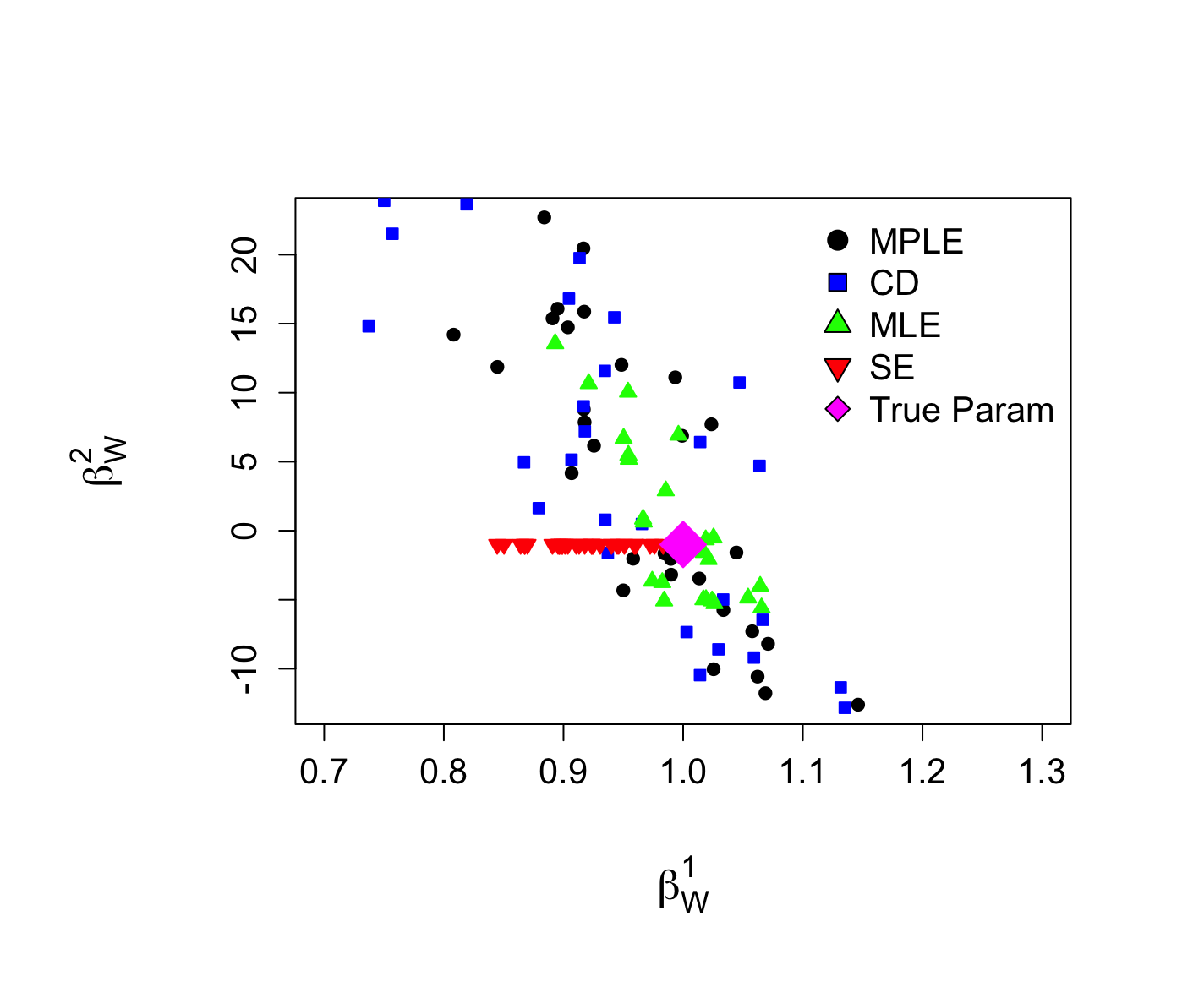
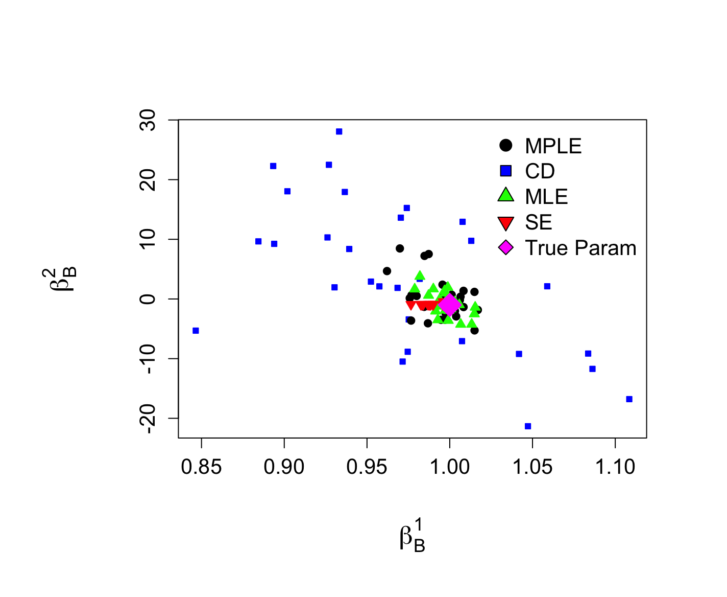
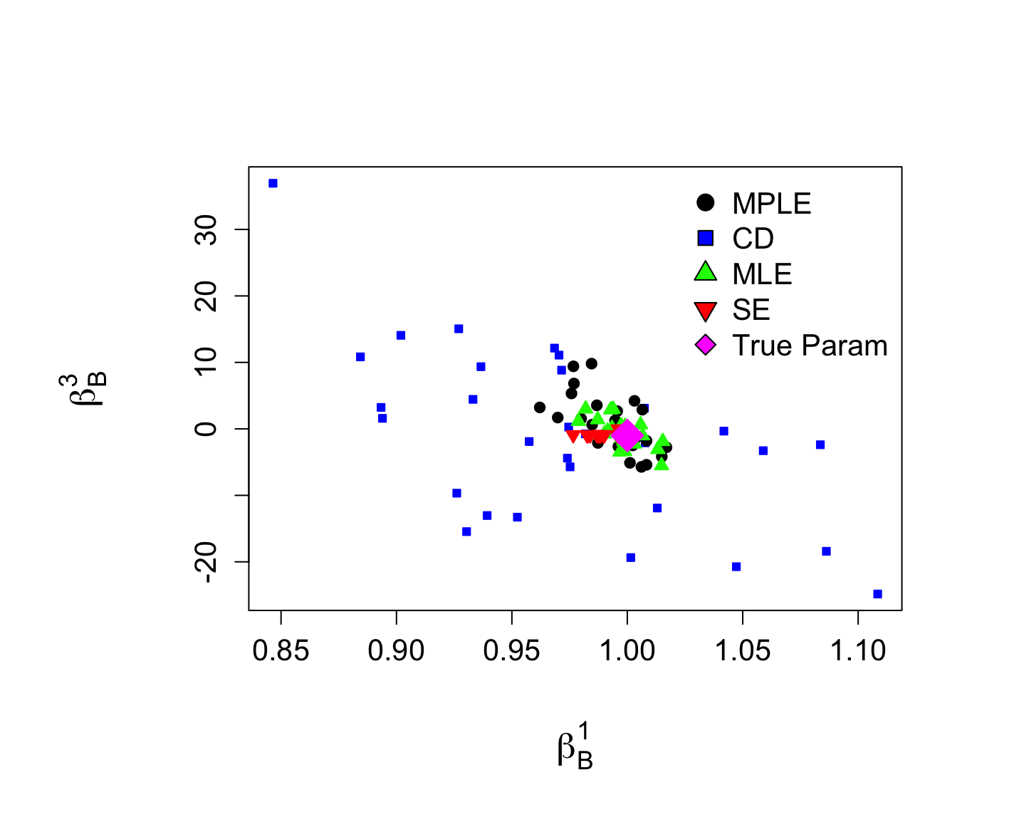
For the same setting, in Table 1 we report the mse squared error (mse) and the standard deviation (std) of the parameter estimates, with respect to the pre-specified true generating parameter values of and . While for the edge parameters and all estimators are very precise, with similar order of precision, for the other parameters the Stein estimator is orders of magnitude more precise than its comparators. The MLE routine in statnet converged roughly of the time; 314 trials were needed to obtain 30 converged estimates for the MLE.
| MLE | MPLE | CD | SE | |||||
| mse | std | mse | std | mse | std | mse | std | |
| 1.88e-3 | 2.58e-3 | 6.62e-3 | 8.30e-3 | 1.32e-2 | 1.87e-2 | 8.73e-3 | 6.57e-3 | |
| 34.9 | 51.9 | 126 | 139 | 198 | 239 | 4.09e-3 | 3.01e-3 | |
| 8.31e-5 | 1.19e-4 | 2.09e-4 | 3.23e-4 | 4.66e-3 | 5.37e-3 | 8.38e-5 | 1.28e-5 | |
| 4.18 | 5.30 | 12.2 | 23.0 | 169 | 203 | 2.07e-2 | 5.57e-2 | |
| 4.47 | 6.03 | 17.7 | 29.1 | 167 | 277 | 4.23e-2 | 1.74e-2 | |
In further exploration we found that the Stein estimator performs reliably well, and as long as the number of vertices in each block is not too small. In particular the Stein estimator appears to be less sensitive towards sparsity than the other methods tested. Moreover, the computational runtime for the Stein estimator is about two orders of magnitude smaller that that for maximum likelihood estimation.
4 Convergence analysis
In order to be rigorous about the dependency structure of the constants and to derive asymptotic results from our error bounds, we work in the following setting: We have a sequence of random graphs , . The graphs all follow a LERGM with the same parameter , but we allow all other quantities involved in the model to depend on , including the vertex set , the partition, and the statistic . As in (1) we denote the number of vertices in a largest block by and write for the number of blocks (using subscripts instead of superscripts for these two quantities for ease of notation). Note that also the domain may depend on . More formally, with denoting the true parameter, we assume that the density of is given by the function defined by
with the statistics if and if and
as well as . In particular that the functions , , , , , now depend on .
Remark 4.1.
Note that, in our setting, estimation is performed based on a single observation and does not involve any other elements from the sequence . Therefore, statistical inference on the parameter is not affected by the dependency structure of the random graphs in , and it is permitted to think of as independently drawn random graphs.
Let us illustrate this point with the Bernoulli random graph . We consider two different ways of defining a sequence that both cover the scenario with vertices:
-
•
Start with and add vertices and the corresponding edges by drawing independent Bernoulli random variables. Thus, for each , and the elements in are dependent.
-
•
For each , draw a new Bernoulli random graph with edges and parameter . Thus, the sequence consists of independent random graphs.
We emphasize that the two definitions above are equivalent when it comes to our statistical inference on the parameter , since our estimator is based on a single observation ; no other random graphs of the sequence is observed for the estimation. We find it most convenient to think of as independent random graphs. However, for the results we develop in this section, we do not need to make any assumptions on the dependency structure of the elements in .
To obtain concentration bounds for Stein estimators we introduce the following model assumption.
Assumption 4.2.
For each we restrict the parameter space of the LERGM as follows: There exist constants independent of such such that and . We denote the corresponding parameter spaces by and .
Here, using the Euclidean norm, we note the implicit dependence that and are of the order and respectively. This assumption is used to bound the second derivatives and from (12) and (13) away from . In [28] this restriction is foregone at the cost of of introducing an assumption on the asymptotic relation between the number of vertices and the number of blocks.
Then a Stein estimator has components
| (17) |
Under Assumption 4.2 the minima in (17) always exist but the minimizing argument may not be unique. In the latter case equals one of the minimizing arguments; we recall that Proposition 3.6 gives theoretical guarantees under conditions on uniqueness of the minima on the model and the observed network.
The next assumption guarantees that changes in the summary statistics occurring from adding or deleting one edge are not too large.
Assumption 4.3.
There exist constants independent of such that
for all , , and as well as
for all , , and .
Similarly as for maximum likelihood estimation, an assumption is needed guaranteeing that the covariance matrix is bounded away from 0 asymptotically, in the following sense.
Assumption 4.4.
Assume that there exist independent of such that
for all , where denotes the smallest eigenvalue of a matrix.
Assumption 4.4 guarantees that the representations of the exponential families are minimal, see [8, Chapter 1].
4.1 Concentration bounds
We have the following theorem, for which existence of a Stein estimator is required, but not uniqueness.
Theorem 4.5.
Proof.
We start with the within-block edges. Parts of this proof follow along the lines of [30, Theorem 3.2.5]. Define
Let , then,
As is a Stein estimator, we have
Since for the true parameter , by construction we have , a Taylor expansion around yields that for
by Assumptions 4.2, 4.4 and 4.3. Thus, with the Markov inequality and Lemma A.3 we obtain
for constants which are independent of and , using that . Therefore, for , with probability at least , we have
Using that for gives the first estimate from the statement of the theorem. The statement for the between-block edges follows analogously, noting that for . ∎
Remark 4.6.
Remark 4.7.
The constants and in Theorem 4.5 can be calculated explicitly. Thus we can obtain non-asymptotic concentration bounds, based on just one observation and a corresponding estimator . Then all quantities in the statement of Theorem 4.5 no longer depend on . and we have the following result: For , under Assumptions 4.2 and 4.3 (adapted to the setting of just a single random graph), with probability at least ,
Remark 4.8.
While no related results for Stein estimators are available, it is possible to compare our results to related results obtained for maximum likelihood estimators. In Corollary 1 in [26], a concentration inequality is obtained for the maximum likelihood estimator in the special case of a model with edges and geometrically weighted edgewise shared partners. For the comparison it is useful to rephrase Theorem 4.5 in terms of ; for any , Theorem 4.5 gives
| (18) |
In contrast, the bound in Corollary 1 of [26] decays exponentially in , but it is not given in a form that could be explicitly evaluated. In Theorem 2.1 of [28] an alternative concentration bound for maximum likelihood estimators is given, under similar conditions as the ones in our paper, but again not in a form that could be evaluated explicitly. The result is obtained under the regime that the dimensions and of the parameter spaces grow at least as fast as . Our bound also allows for the dimensions to grow logarithmically in , but this is not a requirement for it to be valid.
4.2 Asymptotic normality
For standardisation to obtain asymptotic normality, we introduce a matrix for the within-block parameters,
| (19) |
and an analogous matrix for the between-block parameters. Define the deterministic quantities
and
as well as the eigenvalues
For the -Wasserstein distance between two -valued random vectors , is
where the infimum is taken with respect to all probability measures on with marginals , . Moreover, we have the dual respresentation of given by
In particular, The following bounds require existence, but not uniqueness, of Stein estimators.
Theorem 4.9.
Remark 4.10.
Remark 4.11.
We now prove Theorem 4.9.
Proof.
We start with the within-block edges. A Taylor expansion gives
where denotes the th component of a vector. Reorganizing terms yields
Therefore,
As
for all , the matrix is positive semi-definite. For a positive semi-definite matrix , we have that . Using Weyl’s inequality we obtain that
Moreover we have
In addition,
where we used Assumption 4.3 and . Therefore,
Now, we have . Lemma B.2, proved in Appendix 4.2 using a Wasserstein bound from [6] based on Stein’s method, yields
for all . The result for the between-block parameter follows with similar computations. ∎
Remark 4.12.
The next assumptions are used for asymptotical guarantees.
Assumption 4.13.
Assume that there exist independent of such that as well as for all .
Assumption 4.14.
Assume that the random vectors
and
converge to in probability as .
Theorem 4.15.
Proof.
We start with the within-block edges. We define
It follows as in the proof of Theorem 4.5 that for any
for a constant independent of and . Since , this implies that the sequence
| (20) |
is tight. Moreover, by Markov’s inequality, for any
we used that . This implies that we also have
for any . The term above converges to under the assumptions of the theorem. Thus,
| (21) |
as , where denotes convergence in probability. As in the proof of Theorem 4.9, we write
We now investigate term by term. From Lemma B.2 we obtain that
as . Moreover, by Assumption 4.13,
as where we used (21) and the tightness of (20). Finally, with similar calculations as in the proof of Theorem 4.9,
using again the tightness of (20) and assumptions made in the statement of the theorem. Slutzky’s lemma together with Assmption 4.14 then gives the result. The reasoning for the between-block edges is exactly the same. ∎
Remark 4.16.
This section provides theoretical guarantees under explicit conditions which could be checked in principle. However, verifying Assumptions 4.4, 4.13 and 4.14 for instance for the models from Example 3.8 seems to be challenging; this also applies to the corresponding conditions in [28]. If the sequence is bounded and if the number of different statistics is finite, one can verify Assumptions 4.4 and 4.13 computationally. Moreover, in the case where corresponds to the number of blocks and all blocks have the same size and statistics, Assumption 4.14 is just the weak law of large numbers. However, our assumptions 3.4 and 3.7 are easier to check.
Remark 4.17.
In [28], bounds on the distance to normal are obtained for maximum likelihood estimators, under slightly different but related assumptions. Assumptions 1 and 3 in [28] quantify the growth of the summary statistics with respect to number of vertices in each block, partly in relation to a function of the largest eigenvalue of the Fisher information matrix. Assumptions 2 and 4 depend on a choice of which is thought of as small. The normal approximation, Theorem 2.5, in [28] assumes again that the dimension of the parameter space is at least an assumption which is not required for our results and which may not always be natural.
Appendix A Auxiliary results for Section 4.1
We give a result from [9]. Let be a finite set and be a random vector where each takes values in . Also, let , be the sigma-fields generated by and the trivial sigma-field. Moreover, let where and for , be any coupling of the conditional distributions of and . Therefore, is probability measure on . Now define the upper triangular matrix through
| (22) | ||||
where is distributed according to . Note that is a random matrix whose entries are all positive. We define the deterministic matrix through .
For a function we define the vector by letting the th entry of be the variation of at given by
| (23) |
In Lemma A.3 we apply Theorem A.1 to the random graph and therefore have . Before we derive the uniform concentration inequality, we work out a combinatorial upper bound on the variation of the function to which we will apply Theorem A.1.
Lemma A.2.
Suppose that Assumption 4.3 is satisfied. We have that for
for each , where the variation is understood with respect to the argument with an arbitrary ordering of the edges. Moreover, for , and ,
Proof.
We start with the within-block edges. First note that
We tackle the first variation in the display from above. There are at most components of the variation which are not zero. We denote by the Hamming distance on a graph. For any with we compute
each component in is bounded by
Note that we can remove the sum over as the edge in which and differ will be part of at most one block; thus the terms corresponding to all other blocks cancel. Therefore, we have
In the same manner we find
which gives
For the between-block edges, one can proceed in the exact same way with the difference being that there are at most non-zero elements in the variations and , where now . Moreover, the number of elements in , is at most equal to . This gives the bound from the statement of the lemma. ∎
We introduce the Orlicz norm for a real random variable by , where is a convex function with . It is straightforward to see that implies . We will only make use of the function and denote the corresponding Orlicz norm by . Now we can prove the following lemma.
Lemma A.3.
Suppose that Assumption 4.3 is satisfied. Then, for each and there is a constant which is independent of and such that
Proof.
We start with the within-block edges. For let
Note that with the choice
where is the matrix defined in (22) with respect to (for an arbitrary ordering of the edges), we have
where we used Theorem A.1 and therefore . In [28] it is shown that one has . This together with Lemma A.2 implies
Now, the maximal inequality [30, Theorem 2.2.4] implies that
where we used that the covering number with respect to -balls of is bounded above by . Note also that we calculated the constant from [30, Theorem 2.2.4] explicitly. We are left with handling the integral, note that . Then note that the argument inside the logarithm is smaller than if and only if . Therefore, the integral can be bounded by
where we used the inequality for the second estimate. The first integral above can be calculated and is equal to , the second integral can be bounded by
Putting the corresponding terms in the constant and using gives the estimate from the statement of the theorem. The statement for the between-block edges follows analogously. ∎
Appendix B Auxiliary results for Section 4.2
Similarly as [2], our results employ a Wasserstein bound from [6]. Let be independent -valued random vectors such that , , and .
Theorem B.1 ([6, Theorem 5]).
Let Under the above assumptions we have for
where .
Lemma B.2.
Suppose Assumption 4.3 holds. Let , for . Then, for each we have
Proof.
We start with the within-block edges, applying Theorem B.1 to the -valued random vectors
for . Note that all assumptions of Theorem B.1 are easily satisfied as we have a discrete distribution and edges from different blocks are independent. First note that
since edges from different blocks are independent and . We have
where we used that for a positive semi-definite matrix , Weyl’s inequality as well as Assumption 4.3. In a similar way one finds
and
Theorem B.1 then immediately yields the bound
Using that several quantities above are integer-valued, and , the concavity of the function gives the result. ∎
Acknowledgements
This research was funded, in part, by the UKRI EPSRC grants EP/T018445/1, EP/R018472/1, as well as EP/X002195/1 and EP/Y028872/1. For the purpose of Open Access, the authors have applied a CC BY public copyright licence to any Author Accepted Manuscript version arising from this submission. WX acknowledges support from EPSRC grant EP/T018445/1 and the support from the DFG EXC number 2064/1, Project number 390727645.
References
- [1] A. Anastasiou, A. Barp, F.-X. Briol, B. Ebner, R. E. Gaunt, F. Ghaderinezhad, J. Gorham, A. Gretton, C. Ley, Q. Liu, et al. Stein’s method meets computational statistics: A review of some recent developments. Statistical Science, 38(1):120–139, 2023.
- [2] A. Anastasiou and R. E. Gaunt. Wasserstein distance error bounds for the multivariate normal approximation of the maximum likelihood estimator. Electronic Journal of Statistics, 15(2):5758–5810, 2021.
- [3] A. Asuncion, Q. Liu, A. Ihler, and P. Smyth. Learning with blocks: Composite likelihood and contrastive divergence. In Proceedings of the Thirteenth International Conference on Artificial Intelligence and Statistics, pages 33–40. JMLR Workshop and Conference Proceedings, 2010.
- [4] E. C. Barry C. Arnold and J. M. Sarabia. A multivariate version of Stein’s identity with applications to moment calculations and estimation of conditionally specified distributions. Communications in Statistics - Theory and Methods, 30(12):2517–2542, 2001.
- [5] J. Besag. Spatial interaction and the statistical analysis of lattice systems. Journal of the Royal Statistical Society: Series B (Methodological), 36(2):192–225, 1974.
- [6] T. Bonis. Stein’s method for normal approximation in Wasserstein distances with application to the multivariate central limit theorem. Probability Theory and Related Fields, 178(3):827–860, 2020.
- [7] I. Branislav, M. Haifeng, M. Dijana, et al. A survey of gradient methods for solving nonlinear optimization. Electronic Research Archive, 28(4):1573–1624, 2020.
- [8] L. D. Brown. Fundamentals of statistical exponential families with applications in statistical decision theory. IMS Lecture Notes —Monograph Series, 9:i–279, 1986.
- [9] J. R. Chazottes, P. Collet, C. Külske, and F. Redig. Concentration inequalities for random fields via coupling. Probability Theory and Related Fields, 137:201–225, 2007.
- [10] B. Ebner, A. Fischer, R. E. Gaunt, B. Picker, and Y. Swan. Point estimation through Stein’s method. arXiv preprint arXiv:2305.19031, 2023.
- [11] A. Fischer, R. E. Gaunt, and Y. Swan. Stein’s method of moments for truncated multivariate distributions. arXiv preprint arXiv:2312.09344, 2023.
- [12] A. Fischer, R. E. Gaunt, and Y. Swan. Stein’s method of moments on the sphere. arXiv preprint arXiv:2407.02299, 2024.
- [13] J. K. Harris. An Introduction to Exponential Random Graph Modeling. Sage Publications, 2013.
- [14] D. R. Hunter, M. S. Handcock, C. T. Butts, S. M. Goodreau, and M. Morris. ergm: A package to fit, simulate and diagnose exponential-family models for networks. Journal of Statistical Software, 24(3):1–29, 2008.
- [15] D. R. Hunter, M. S. Handcock, C. T. Butts, S. M. Goodreau, and M. Morris. ergm: A package to fit, simulate and diagnose exponential-family models for networks. Journal of Statistical Software, 24(3):1–29, 2008.
- [16] P. N. Krivitsky. ergm.multi: Fit, Simulate and Diagnose Exponential-Family Models for Multiple or Multilayer Networks. The Statnet Project (https://statnet.org), 2024. R package version 0.2.1.
- [17] P. N. Krivitsky, D. R. Hunter, M. Morris, and C. Klumb. ergm 4: New features for analyzing exponential-family random graph models. Journal of Statistical Software, 105(6):1–44, 2023.
- [18] D. Lusher, J. Koskinen, and G. Robins. Exponential Random Graph Models for Social Networks: Theory, Methods, and Applications. Cambridge University Press, 2013.
- [19] G. Mijoule, M. Raič, G. Reinert, and Y. Swan. Stein’s density method for multivariate continuous distributions. Electronic Journal of Probability, 28:1–40, 2023.
- [20] S. Mukherjee. Degeneracy in sparse ERGMs with functions of degrees as sufficient statistics. Bernoulli, 26(2):1016 – 1043, 2020.
- [21] S. Mukherjee and Y. Xu. Statistics of the two star ERGM. Bernoulli, 29(1):24–51, 2023.
- [22] M. Raič. A multivariate Berry–Esseen theorem with explicit constants. Bernoulli, 25(4A):2824–2853, 2019.
- [23] G. Reinert and N. Ross. Approximating stationary distributions of fast mixing Glauber dynamics, with applications to exponential random graphs. The Annals of Applied Probability, 29(5):3201–3229, 2019.
- [24] M. Schweinberger and M. S. Handcock. Local dependence in random graph models: characterization, properties and statistical inference. Journal of the Royal Statistical Society Series B: Statistical Methodology, 77(3):647–676, 2015.
- [25] M. Schweinberger, P. N. Krivitsky, C. T. Butts, and J. R. Stewart. Exponential-family models of random graphs. Statistical Science, 35(4):627–662, 2020.
- [26] M. Schweinberger and J. Stewart. Concentration and consistency results for canonical and curved exponential-family models of random graphs. The Annals of Statistics, 48(1):374–396, 2020.
- [27] T. A. Snijders. Markov chain Monte Carlo estimation of exponential random graph models. Journal of Social Structure, 3(2):1–40, 2002.
- [28] J. R. Stewart. Rates of convergence and normal approximations for estimators of local dependence random graph models. arXiv preprint arXiv:2404.11464, 2024.
- [29] A. Stivala, G. Robins, and A. Lomi. Exponential random graph model parameter estimation for very large directed networks. PloS one, 15(1):e0227804, 2020.
- [30] A. W. van der Vaart and J. A. Wellner. Weak Convergence and Empirical Processes: With Applications to Statistics. Springer Series in Statistics. Springer International Publishing, Cham, 2nd ed. 2023. edition, 2023.
- [31] S. Wasserman and K. Faust. Social Network Analysis: Methods and Applications. Cambridge University Press, 1994.
- [32] G. G. V. Yon, A. Slaughter, and K. de la Haye. Exponential random graph models for little networks. Social Networks, 64:225–238, 2021.
