Micro Blossom: Accelerated Minimum-Weight Perfect Matching Decoding for Quantum Error Correction
Abstract.
Minimum-Weight Perfect Matching (MWPM) decoding is important to quantum error correction decoding because of its accuracy. However, many believe that it is difficult, if possible at all, to achieve the microsecond latency requirement posed by superconducting qubits. This work presents the first publicly known MWPM decoder, called Micro Blossom, that achieves sub-microsecond decoding latency. Micro Blossom employs a heterogeneous architecture that carefully partitions a state-of-the-art MWPM decoder between software and a programmable accelerator with parallel processing units, one of each vertex/edge of the decoding graph. On a surface code with code distance and a circuit-level noise model with physical error rate , Micro Blossom’s accelerator employs parallel processing units to reduce the worst-case latency from to and reduce the average latency from to when .
We report a prototype implementation of Micro Blossom using FPGA. Measured at and , the prototype achieves an average decoding latency of at a moderate clock frequency of . Micro Blossom is the first publicly known hardware-accelerated exact MWPM decoder, and the decoding latency of is 8 times shorter than the best latency of MWPM decoder implementations reported in the literature.
1. Introduction



[potential speed up]
Quantum error correction (QEC) plays an important role in building fault-tolerant quantum computers. It requires a decoder that processes syndromes, potentially measured times per second, to discover qubit errors timely, within a microsecond (AI, 2023) in the case of implementing fault-tolerant logical gates (Holmes et al., 2020). For surface codes, an important class of QEC codes, the most-likely error decoding problem can be formulated as a Minimum-Weight Perfect Matching (MWPM) problem (Dennis et al., 2002) associated with a syndrome graph (Wu et al., 2022), under the assumption of a noise model of independently distributed bit and phase flips, and can be solved by the famous blossom algorithm (Edmonds, 1965; Kolmogorov, 2009).
In recent years, many MPWM decoder implementations have been implemented in response to high throughput and low latency requirements. Sparse Blossom (Higgott and Gidney, 2025) and Parity Blossom (Wu and Zhong, 2023) reduce the time complexity of MWPM decoding by adapting the blossom algorithm to work on the decoding graph. Fusion Blossom (Wu and Zhong, 2023) improves throughput by using multiple cores to process blocks of syndrome measurement rounds in parallel. None of these exact MWPM decoders achieve a decoding latency close to a microsecond or leverage any hardware acceleration. In fact, it is believed (Vittal et al., 2023) that the blossom algorithm (Edmonds, 1965; Kolmogorov, 2009), which underpins all these MWPM decoders, is too complex for hardware acceleration. Not surprisingly, many have resorted to less accurate decoders that approximate MWPM decoding (Vittal et al., 2023; Liyanage et al., 2023; Alavisamani et al., 2024), causing 1.7x (Liyanage et al., 2023) or even 13.9x (Alavisamani et al., 2024) more logical errors at code distance and physical error rate .
In this work, we present the first publicly known exact MWPM decoder that achieves sub-microsecond latency, called Micro Blossom. It is also the first publicly known exact MWPM decoder with hardware acceleration. Micro Blossom builds on ideas from recent fast decoders, namely (Wu and Zhong, 2023; Higgott and Gidney, 2025), to implement the blossom algorithm and support stream decoding. Micro Blossom carefully partitions the blossom algorithm between software and a programmable accelerator of parallel processing units (PUs), one corresponding to each vertex and edge in the decoding graph (§3). It implements the primal phase of the blossom algorithm in software that flexibly handles complex data structures. It implements the dual phase in the programmable accelerator that exploits the finest-grained parallelism of the decoding graph in vertices and edges (§4). To reduce the expensive software-hardware interaction, Micro Blossom uses parallel PUs to resolve common Conflicts without involving the primal phase on the CPU (§5). To support low-latency stream decoding, Micro Blossom performs round-wise fusion with the parallel PUs in the accelerator (§6).
Using SpinalHDL (Papon and Xiao, 2023), we implement a parameterized prototype of Micro Blossom that takes an arbitrary decoding graph as input and produces synthesizable Verilog code (§7). When running the accelerator on a Xilinx Versal VMK180 FPGA, our prototype achieves an average decoding latency of for code distance and physical error rate in a circuit-level noise (§8). It is the first publicly known MWPM decoder with sub- latency, 8x shorter than the best reported (Higgott and Gidney, 2025), for the same code distance and noise model. We note that the largest surface code reported in QEC physical experiments is (Acharya et al., 2024). We also note that Micro Blossom can support even larger for sub- latency if more resources are available, e.g., larger FPGA, and if higher clock frequency is feasible, e.g., using ASIC, as analyzed in §8.4.
In summary, we make the following contributions:
-
•
We design a heterogeneous architecture for scalable, real-time, and exact MWPM decoding for QEC.
-
•
We parallelize the blossom algorithm at the vertex and edge levels, which improves both the worst-case and average decoding latency.
-
•
We demonstrate the first publicly known sub- average latency of MWPM decoding on a prototype using FPGA for surface code of .
Our implementation of Micro Blossom is open-source and available from (Wu, 2024).
2. Background
Quantum Error Correction (QEC) Codes
A QEC code encodes a logical qubit using multiple physical qubits. The surface code is one of the most promising QEC codes, featuring a universal fault-tolerant gate set that enables fault-tolerant quantum computation (Fowler et al., 2012). As shown in 1(a), a distance- surface code consists of data qubits and stabilizers.
Decoding Graph
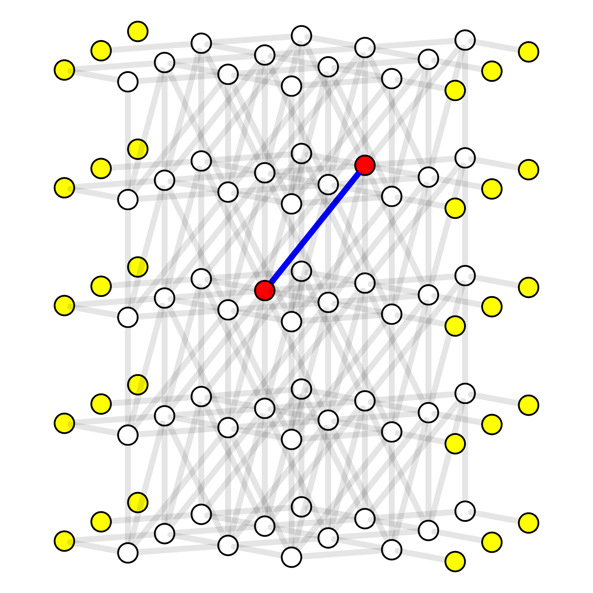
As shown in 1(b), a decoding graph is a weighted graph derived from a code and noise model. Each vertex corresponds to a stabilizer measurement. If the measurement result is flipped, we call the corresponding vertex a defect vertex, marked in red; otherwise, it is a regular vertex marked in white. represents the set of defect vertices. Each edge corresponds to a potential quantum error, with weight calculated from the error probability by . An edge connects the vertices that can detect the corresponding error. Virtual vertices (in yellow) along the code boundary represents the unknown measurements (Wu and Zhong, 2023).
Since stabilizer measurements are noisy, we need measurement rounds to achieve fault tolerance (Gottesman, 2013). The resulting decoding graph is a three-dimensional (3D) graph that contains vertices, as shown in 1(c). Each horizontal layer, which is two-dimensional (2D), corresponds to a measurement round. The edges between layers represent the measurement errors.
Syndrome graph and MWPM Decoder
The set of defect vertices is known as the syndrome. Given the decoding graph and a syndrome, one can derive the syndrome graph, which is a fully connected graph with the vertices being the defect vertices from the decoding graph. The weight of an edge is computed as the minimum weight of paths in the decoding graph between the two incident defect vertices. The Minimum-Weight Perfect Matching (MWPM) decoder finds the most likely error by finding an MWPM in the syndrome graph. We denote the edges of the syndrome graph as .
Blossom Algorithm
The blossom algorithm leverages Linear Programming (LP) to solve the minimum-weight perfect matching (MWPM) problem (Edmonds et al., 1969). It considers the original MWPM problem as the primal problem: minimizing the total weight where the primal variable is either 1 or 0, indicating whether edge is in the matching. Accordingly, the dual problem maximizes the sum of the dual variables where (Wu and Zhong, 2023). In this dual problem, there is a constraint corresponding to each primal variable (and therefore each edge). When the equality for this constraint holds, the corresponding edge is considered tight.
The blossom algorithm works on both the primal and dual problems. The dual phase, solving the dual problem, changes and creates tight edges; the primal phase, solving the primal problem, changes and determines which tight edges will be in the matching. Intuitively, the blossom algorithm gradually increases the “available budget” () while checking whether a perfect matching solution with a “cost” () exists within the “budget”. The dual phase increases the “budget” while ensuring it does not exceed the minimum required “cost” (by enforcing dual constraints). The primal phase seeks a perfect matching within the allocated “budget”, and negotiates with the dual phase to increase it as needed. The optimality is achieved when the “cost” matches the “budget”.
Three notions from the blossom algorithm are important in this work: blossom, node, and alternating tree. In the context of QEC (Wu and Zhong, 2023), we can inductively define a blossom on the syndrome graph as follows, adapted from (Wu and Zhong, 2023) (Page 4): (i) a defect vertex is a blossom; (ii) an odd number of blossoms connected by tight edges in a circle form a blossom. Apparently, each blossom is associated with a dual variable . A node is a blossom that does not belong to any other blossom according to (ii). Each defect vertex belongs to a unique node, denoted .
The primal phase organizes nodes (and tight edges) into matched pairs and alternating trees. A matched pair consists of two nodes connected by a tight edge with . An alternating tree consists of an odd number of nodes that are connected by tight edges in a tree. In the tree, there are an odd number of tight edges connecting any leaf node to the root. It is called an alternating tree because alternating edges along the path from a leaf to the root are included in the matching with . A single node not matched is also an alternating tree. An example of a matched pair and an alternating tree is shown in Figure 3.
With alternating trees and matched pairs, the primal phase determines how to adjust a dual variable in the dual phase by assigning a direction . When is matched, it sets as ; otherwise, it determines by ’s position in the alternating tree which alternates between from the root () to the leaf (also ) as shown in Figure 3. The dual phase adjusts based on . When , we say it grows (and the node ); when , we say it shrinks (and the node ). When , we say nodes and are growing toward each other.

[example alternating tree]
Fast MWPM Decoders
The blossom algorithm solves the MWPM decoding problem using the syndrome graph (Wu et al., 2022), which is dense with edges. Sparse Blossom (Higgott and Gidney, 2025) and Parity Blossom (Wu and Zhong, 2023) speed up MWPM decoding by adapting the blossom algorithm to solve the MWPM problem on the decoding graph, which is adopted by Micro Blossom.
Parity Blossom conveniently decomposes the blossom algorithm into the primal and dual phases, which is also adopted by Micro Blossom. Parity Blossom implements these in the decoding graph, improving the asymptotic average time complexity to almost linear, but still falls short of sub- decoding latency. As shown in Figure 2, the dual phase takes most of the decoding time of Parity Blossom. Improving the speed of the dual phase is critical for further improving the decoding speed.
[real time decoding]
Why Decoding Latency Matters
Nontrivial fault-tolerant quantum computing requires feedforward from the decoder with a soft deadline (Terhal, 2015), making the decoding a soft real-time problem. The soft deadline comes from implementing logical non-Clifford gates, which are necessary for any universal quantum gate set. For example, implementing a logical gate requires a logical qubit readout as a feedforward signal, as shown in Figure 4. While waiting for the decoded readout, the target qubit accumulates more logical errors. When there is no decoding latency, the data qubit only goes through stabilizer measurement rounds and suffers from a total logical error rate of . If the decoding latency is measured in the number of stabilizer measurement cycles, then the logical error rate of the target qubit effectively becomes roughly . Taking surface code with measurement cycle (AI, 2023) as an example, the effective logical error rate is for Fusion Blossom (Wu and Zhong, 2023), and for the faster but less accurate Union-Find decoder (Liyanage et al., 2024). In this case, although Union-Find decoding has 5x more logical errors than MWPM decoding, it causes fewer logical errors when including latency-induced idle errors.
3. Micro Blossom Architecture
As shown in Figure 5, Micro Blossom is a heterogeneous architecture to solve MWPM decoding for QEC with sub-microsecond decoding latency. It builds on ideas from recent fast decoders: (i) using the decoding graph, instead of the syndrome graph (Wu and Zhong, 2023; Higgott and Gidney, 2025) and (ii) using fusion operations to support stream decoding (Wu and Zhong, 2023). Like these decoders, Micro Blossom also implements the blossom algorithm (Edmonds et al., 1969) and therefore is logically equivalent to them. Micro Blossom, however, advances the state of the art in implementation by realizing vertex and edge level parallelism, while Fusion Blossom (Wu and Zhong, 2023) is effective to coarse-grained parallelism and Parity Blossom (Wu and Zhong, 2023) and Sparse Blossom (Higgott and Gidney, 2025) do not exploit parallelism at all (See §9).

3.1. Overview
Micro Blossom carefully partitions the blossom algorithm between software and hardware. The software handles dynamically sized data structures while the hardware (accelerator) employs a large number of processing units (PUs) with local connectivity. There are two types of stateful PUs: Vertex PU (vPU) and Edge PU (ePU). The accelerator associates a vPU for each vertex and an ePU for each edge in the decoding graph, achieving the finest possible parallelism for graph algorithms. Because decoding graphs vary depending on how physical qubits are grouped into logical qubits and the logical operation, our implementation takes a decoding graph as input and outputs synthesizable Verilog code for the accelerator (§7).
The accelerator in Micro Blossom is programmable with a small instruction set. It carefully decouples the data and control planes. The data plane includes the PUs, which only exchanges data locally, with their immediate neighbors. The syndrome data are loaded to the vPUs, which can be fed with shift registers to minimize routing congestion. Once all syndromes have been loaded and the MWPM solution is determined, the controller outputs the logical correction bits. The control plane consists of a controller, a broadcast network that sends control signals to all PUs, and a convergecast network that collects responses from them. The controller interfaces with the software via memory-mapped registers.
3.2. Key Ideas
Accelerating Dual Phase (§4)
Given that the dual phase is the current speed bottleneck of a software implementation, as shown in Figure 2, we accelerate it using parallel PUs, organized according to the decoding graph. The key algorithmic innovation behind this is a parallel variant of Parity Blossom (Wu and Zhong, 2023) with which the dual phase is implemented by parallel PUs, each of which only uses its local state and that of its immediate neighbors. The key is to distribute the information of Covers down to per-vertex data structures (implemented as per-vPU state). This key idea improves the worst-case time complexity from of the fastest sequential algorithm (Higgott and Gidney, 2025) to using parallel resources.
Accelerating Primal Phase (§5)
Although the most time-consuming dual-phase operations are offloaded to the hardware, the CPU still has to do at least one read and write for every defect vertex in the primal phase. The interaction between the CPU and the hardware becomes the bottleneck, leading to an average time complexity of with a large constant factor of hundreds of nanoseconds per interaction. Our key idea is to find a simple component of the primal phase that can be efficiently parallelized in the hardware accelerator. We prove that if any error occurs alone, it is offloaded to the hardware accelerator in time. Given the independence of the errors, the average decoding time is reduced from to , eliminating the interaction for all first-order errors and thus reducing the interaction between the CPU and the hardware.
Round-wise Fusion for Streaming (§6)
Multiple rounds of stabilizer measurements constitute a stream as one round becomes available every . To reduce decoding latency, instead of waiting for all rounds of a syndrome, the decoder can process a round as soon as it arrives and fuse their results progressively, as demonstrated in (Wu and Zhong, 2023). Micro Blossom leverages vertex-level parallelism in such fusion operations to further accelerate them for fine-grained stream decoding within measurement round. This round-wise fusion complements the coarse-grained fusion of prior work (Wu and Zhong, 2023). Importantly, we combine round-wise fusion with the parallel primal phase acceleration. When decoding is faster than the measurement rate, round-wise fusion further reduces the average decoding latency from to .
4. Accelerating Dual Phase
| Operation | Arguments | Description in Parity Blossom | Local Algorithm on Parallel PUs in Micro Blossom | |||||
|---|---|---|---|---|---|---|---|---|
| set Direction | , | update the direction of node , | each vPU updates the direction if | |||||
| grow | length | grow the Covers of nodes by |
|
|||||
| update Cover | — | update the boundary of the Covers |
|
|||||
| merge Cover | nodes | merge the Covers of as the Cover of | each vPU replaces every with in | |||||
| split Cover | node | split ’s Cover into individual Covers of |
|
|||||
| detect Conflict | — |
|
|
In this section, we describe how to accelerate the dual phase using parallel PUs. The key insight is that certain operations in Parity Blossom (Wu and Zhong, 2023) can be parallelized using the Covers of the nodes. We can use parallel PUs to (1) maintain the Covers when performing a dual-phase operation, and (2) implement these operations using the local state.
We first provide background on Parity Blossom in §4.1, describe a new algorithm design that parallelizes dual-phase operations at the vertex level in §4.2, and present a more resource-efficient version of the algorithm in §4.3.
4.1. Background
Parity Blossom (Wu and Zhong, 2023) is based on a geometric interpretation of the decoding graph in which any two points in the graph have a non-negative distance.
The algorithm associates each defect vertex with a set of points called Circle, , with being the center and a radius of (Appendix D (Wu and Zhong, 2023)). We say two Covers are neighbors if their associated vertices are neighbors on the decoding graph.
Parity Blossom associates a node with a set of points called Cover, which is the union of the above Circles of defect vertices in the node, i.e., .
Finally, the algorithm reduces the dual-phase operations to the manipulations of its Covers. We have Theorem: Tight Edge Detection (Cover) (Wu and Zhong, 2023) that implies there exists a tight edge between nodes and . The dual phase of Parity Blossom maintains the Covers of the nodes and uses them to detect situations when it can no longer adjust the dual variables without violating any dual problem constraint, called Obstacles. Once the dual phase detects an Obstacle, the algorithm switches to the primal phase to resolve it.
There are two types of Obstacles, as defined in (Wu and Zhong, 2023) as (2a) and (2b). The first corresponds to the constraint (2a) when the dual variable of a node is already 0 but is still shrinking: . This type of Obstacle occurs rarely and can be handled efficiently using a priority queue on the CPU (Kolmogorov, 2009; Higgott and Gidney, 2025). The second type corresponds to constraint (2b) and occurs more frequently, when two nodes ( and ) are growing toward each other () while there is already a tight edge between them in the syndrome graph (). We call this type of Obstacle Conflict. A Conflict indicates an edge connecting the two nodes in the syndrome graph has become tight.
The first three columns of Table 1 describe all dual-phase operations in (Wu and Zhong, 2023). The first five operations update the Covers while the last operation detects Conflicts.
An astute reader may realize that Parity Blossom is Cover -parallel, although the implementation reported in (Wu and Zhong, 2023) did not exploit this. Because Covers are only associated with defect vertices and defect vertices appear randomly on the decoding graph, manipulations of a Cover may require information about non-neighboring Covers, which would require non-local connectivity between vertices if one tries to achieve vertex-parallelism by associating a PU with each vertex like Micro Blossom.
4.2. Algorithm of Parallel Dual-phase Operation
The key idea of Micro Blossom toward achieving vertex-level parallelism is to maintain per-vertex information that is updated locally so that manipulations of a Cover will only require information associated with the vertices and edges within the Cover. We use vertices to store the information of Covers in a distributed manner while only storing the edge weights on the edges. The algorithm is formally described in Column 4 of Table 1.
Algorithm: Parallel Dual Operations Dual-phase operations can be implemented in parallel using information local to PUs, according to Table 1 (Column 4).
We next succinctly present the mathematical notions and theorems behind this algorithm.
Definition: Residual Distance. Given a vertex and a defect vertex from a decoding graph, we define the Residual Distance as
Definition: Residue, Touches and Nodes. Given a vertex , we define the following states: Residue , Touches , and Nodes .
In Micro Blossom, each vPU maintains the Residue, Touches and Nodes of the corresponding vertex. In addition, it also records all the directions . The complete PU state is shown in Table 2.
Together, the per-vertex states maintained by all vPUs constitute a distributed description of the Covers. Each vPU knows whether its vertex belongs to the Cover of a node (), and if so, how far it is from the nearest boundary (). An example is shown in Figure 6, where the vertex’s state provides information on Covers that includes it.
| PU | Full State (§4.2) | Compact State (§4.3) | Compact Values | ||
|---|---|---|---|---|---|
| Vertex () | Touches () | unique-Touch () | or | ||
| Nodes () | unique-Node () | or | |||
| Residue () | |||||
|
Direction () | +1, -1, 0 | |||
| Is Defect () | |||||
| Is Boundary () | |||||
| Index () | |||||
| Edge () | Weight () | ||||
We prove the following theorems. The first implies that all Conflicts can be detected locally on each ePU of only using information local to and its incident vertices. The second implies that the length of growth can be found locally for each vPU and ePU.
Theorem: Conflict Detection. There is a Conflict between nodes and .
The accelerator computes the right side of in the above theorem in two steps: (i) each ePU computes for every in parallel and reports the result; (ii) the convergecast tree aggregates results from all ePUs. We note that is local to the ePU associated with ; , , and are local to the vPU associated with , which is incident to .
When an ePU detects a Conflict in Step (i), it reports , , , , , where and . and exist due to the definition of . The convergecast tree picks an arbitrary Conflict (and its report) out of all reported. The convergecast tree consists of multiplexers and incurs an latency. In this way, when there exists any Conflict, the accelerator reports at least one of them and thus implements the dual phase (Wu and Zhong, 2023).
Theorem: Local Length to Grow. We can find a Conflict after iterative “grow” operations of the following length using only local information for each vertex and edge:
In the accelerator, vPUs compute the left of in the above theorem while ePUs compute the right, both using local information. The PUs report their results via the convergecast tree to compute the minimum , which consists of comparators and incurs an latency.
Together, the above two theorems indicate that per-vertex states can replace Covers to detect Conflicts in the implementation of the blossom algorithm. Concretely, they lead to the algorithm for the six dual-phase operations with local information described in Table 1.
4.3. A More Resource-Efficient Algorithm
Although the local algorithm in Table 1 implements all dual-phase operations with vertex and edge-level parallelism and using only local information, it requires a large per-vertex state for hardware implementation: both and require memory. In order to reduce resource usage for each vPU, we further simplify the algorithm so that a vPU only stores a unique Touch and Node for its vertex.
Definition: unique Touch and Node. The unique-Touch is a touch vertex whose node has the maximum , and the unique-Node is the node of .
By maintaining a single touch and node , we reduce the state of vPU as summarized in Table 2 and the instruction set that operates on it in Table 3.

Instruction set
As shown in Table 3, we design a compact instruction set that represents each dual-phase operation in Table 1. Another inefficiency in §4.2 is that the “split Cover” operation requires each vPU to maintain the hierarchical structure of the blossom. We mitigate this problem by storing the blossom structure in the CPU and using a single setCover(, ) instruction to implement both “merge Cover” and “split Cover” operations. Each vPU simply set if or upon receiving “set Cover”.
Compact PUs
We implement this resource-efficient algorithm using a compact state per vertex and edge as shown in Table 2 and combinational logic with a fixed CPI (clock per instruction) of 1. This combinational logic takes the current state from the registers of its neighboring vertices and edges. Then it outputs the next state that is captured by the registers and fed as input in the next clock cycle. All PUs share the same clock and run synchronously. In surface code, the number of registers or gates scales with , as detailed in §8.4.
| Instruction | Arguments | Instruction Word (32 bits) |
|---|---|---|
| reset | — | | |1001|00| |
| set Direction | | S [31:17] |dir [16:15] 0|00| |
|
| grow | | l [31:6] |1101|00| |
|
| set Cover | | C [31:17] | S [16:2] |01| |
|
| find Conflict | — | | |0001|00| |
| load Defects | custom | | custom[31:6] |0111|00| |
5. Accelerating Primal Phase
As described in §4, Micro Blossom accelerates the dual phase with parallel PUs while keeping the primal phase in software, running on a CPU. As a result, the CPU and accelerator frequently interact during the decoding process, which significantly contributes to the decoding latency. One major source of such interactions is when the dual phase (running on the accelerator) detects a Conflict, the primal phase (running on the CPU) must resolve it. We reduce the frequency of such interactions by postponing the handling of a common type of Conflicts and derive their matchings in parallel. We first provide background (§5.1) and demonstrate a resource-efficient, time implementation of detecting and handling such Conflicts on parallel PUs (§5.2).
5.1. Background
When the dual phase detects a Conflict, the primal phase manipulates the alternating trees and the matched pairs following a set of rules (Kolmogorov, 2009). It does three things. (i) it changes some primal variables . (ii) It changes the direction () for the nodes involved (See §2 Blossom Algorithm). (iii) it may create new blossoms or expand existing blossoms. In Micro Blossom, the primal phase (running the CPU) sends the “set Direction” and “set Cover” instructions to the accelerator as a consequence of (ii) and (iii), respectively.
There is a special type of Conflict that requires much simpler primal phase operations. We call them isolated Conflicts. Isolated Conflicts are results of isolated errors whose neighboring error sources are normal, as shown in 7(a) where errors are represented by blue edges in the decoding graph. With ever-improving physical qubits, isolated errors are common. Importantly, when the physical error rates vary little, i.e., , an isolated physical error always leads to one isolated Conflict. An isolated Conflict happens when the Cover of a node incident of an isolated error (represented by edge ) grows into that of the other node incident of , which can be either a defect vertex (7(b)) or a virtual vertex (7(c)), before they touch any other Covers. When an isolated Conflict happens, the primal phase’s three operations are much simpler. (i) it sets to , where is the edge between and in the syndrome graph. (ii) it sets (and in the case of 7(b)) to . The primal phase does not do anything for (iii). Our key insight is that if an isolated Conflict remains isolated at the end of the algorithm, it can be incorporated into the final MWPM trivially: , the edge between and in the syndrome graph, should be in the MWPM. That is, the accelerator does not need to report an isolated Conflict at all. When one of the involved Covers touches another Cover during the course of the algorithm, leading to a non-isolated Conflict, the accelerator will report this new Conflict to the CPU, which will discover the previously unreported Conflict from the report.
5.2. Accelerated Handling of Isolated Conflict


We next describe how Micro Blossom detects and handles some common isolated Conflicts using parallel PUs, without invoking the CPU. Because not all isolated Conflicts can be detected by PUs using local information only, we must narrow down to those that can be.
Parallel ePU Logic for Detecting Isolated Conflicts
For an ePU to detect if an isolated Conflict happens on its edge , it must tell if and are both nodes and and touch other Covers. In general, this is impossible only with information local to the ePU (the local states of vPUs of its incident vertices). Our key idea is to only consider those isolated Conflicts in which whether and touch other Covers can be detected using information local to each ePU. We have identified two kinds of such isolated Conflicts.
The first kind is illustrated by 7(b) where an isolated error happens away from the surface code boundary and leads to a pair of defect vertices whose other neighbors are non-defect. We define indicates whether is tight. indicates whether is the only tight edge incident to , which can be computed by ’s vPU. We detect such isolated Conflicts using the following condition.
| (1) |
However, the above condition is not effective for an edge on the boundary of the surface code, as illustrated by 7(c). This is because likely also touches the neighboring regular vertices . Thus, we have to detect isolated Conflicts using the vPU states from all , which is more expensive than Equation 1.
| (2) |
In summary, in Micro Blossom, ePUs corresponding to regular and boundary edges use Equation 1 and Equation 2 as sufficient conditions to detect isolated Conflicts in parallel.
Parallel Handling of Isolated Conflict
Once an ePU detects an isolated Conflict, its detection logic is true, which temporarily signifies that the corresponding edge in the syndrome graph should be included in the matching and should be set as 1. It sets and to so there will be no change to and . These correspond to primal operations (i) and (ii) described in §5.1.
During the process of the algorithm, if another Cover touches that of (or that of in the case of 7(b)), a non-isolated Conflict happens. will turn false and some ePU will report the new Conflict to the primal phase on the CPU, which will also find out the unreported Conflict on .
When the algorithm ends, if the Conflict on edge remains isolated, the accelerator trivially includes , the edge between and in the syndrome graph, in the MWPM.
6. Round-wise Fusion for Stream Decoding
To further reduce decoding latency, Micro Blossom processes the syndrome in a stream manner, starting the decoding process as soon as a measurement round arrives. We provide background on the fusion operation in §6.1, which enables stream decoding. We describe round-wise fusion that performs intra-block fusion to further lower decoding latency, as detailed in §6.2. Additionally, we extend the local Conflict detection algorithm to support round-wise fusion in §6.3.
6.1. Background
As shown in Figure 5, syndrome data for a surface code comes in a series of measurement rounds with a fixed interval (about for superconducting qubits). Stream decoding treats the decoding problem as an incremental optimization problem: instead of waiting for all rounds to solve them as a single batch, stream decoding can start decoding as soon as the first round arrives and incrementally incorporates a newly arrived round into the solution. If properly designed, a stream decoder finds a final solution identical to that of a batch decoder.
Fusion Blossom (Wu and Zhong, 2023) is such a stream decoder based on Parity Blossom and the concept of fusion. It divides the decoding graph into two non-overlapping subgraphs and , and a set of vertices , which form a boundary between and . It finds the MWPMs for and separately using Parity Blossom and fuses them into the MWPM for by considering the boundary vertices . This divide-fusion process can be applied recursively so that Parity Blossom is only invoked on a subgraph of a manageable size. Fusion Blossom differs from other stream decoding methods, such as window decoding (Dennis et al., 2002; Iyengar et al., 2011; Skoric et al., 2023; Tan et al., 2022; Bombín et al., 2023), in that it does not compromise decoding accuracy or introduce redundant computation. In (Wu and Zhong, 2023), the authors considered the smallest subgraphs that consist of multiple measurement rounds.
Micro Blossom adopts the same approach to implement stream decoding but considers a novel, extreme case where consists of all measurement rounds received before the latest, is empty, and the boundary includes vertices in the latest measurement round. We call this strategy round-wise fusion.
6.2. Round-wise Fusion
Round-wise fusion incrementally finds the global MWPM by fusing a newly arrived measurement round into the partial MWPM of previously received rounds. Its global optimality is guaranteed per Fusion Blossom (Wu and Zhong, 2023).
As the accelerator features a array of vPUs, when the first round arrives, the accelerator loads it into the first layer () and solves it. When the second round arrives, the accelerator loads it into the second layer (). It treats the first layer as , the second layer as the boundary , and , and performs the fusion. This process continues until all rounds have been processed.
Micro Blossom implements the above process in time simply by manipulating the vPU state , which indicates whether the associated vertex is a boundary vertex. It sets to true if the vPU is unloaded; as a result, it treats as a virtual vertex in the fusion operation (Wu and Zhong, 2023). Each vPU is assigned a layer ID according to its position in the 3D array. At the outset, of all vPUs is set to true. When a new round of syndrome is available, the controller issues a “load Defects” instruction with the layer ID. Upon receiving this instruction, the vPUs with the matching layer ID load the defect bit and set to false.
To perform the fusion, the only additional logic is in the software (CPU) that breaks all existing matchings with the fusion boundary, which are originally virtual vertices in the newly arrived layer (Wu and Zhong, 2023). Then Micro Blossom continues to resolve the new Conflicts and to find the optimal solution for the fused decoding graph.
6.3. Handling Isolated Conflict
We next extend the parallel detection of isolated Conflicts (§5.2) to round-wise fusion. From §5.2, we know that detecting isolated Conflicts for boundary edges (Equation 2) is more expensive than that for regular edges (Equation 1). Without round-wise fusion, boundary edges are relatively rare and as a result, add little to the overall overhead. However, with round-wise fusion, every edge must be a boundary edge at least once. As a result, the high cost of detecting isolated Conflicts on the boundary edges becomes problematic.
Our key insight toward mitigating this problem is that the logic for boundary edges is complicated because may touch other vertices, i.e., and in 7(c), before touching the Cover of a virtual vertex (). By temporarily reducing the weights of edges connected to the fusion boundary , isolated Conflict likely happens on these edges without interacting with other vertices. Once becomes false, the ePUs restore the original edge weights, ensuring that the final solution remains intact after all vPUs have loaded the syndrome.
Based on the above idea, we design a more resource-efficient logic to detect isolated Conflicts during round-wise fusion, replacing that of Equation 2. For an edge where vertex has a layer ID higher than that of , we define the isolated Conflict condition . First, we define the concept of non-volatile tightness , which ignores temporary tight edges when is still virtual: . Next, we define , which checks if vertex has no non-volatile tight edges surrounding it. The condition holds when is virtual and is a growing node without any non-volatile tight edge incident to .
| (3) |
When the physical error rates vary little, like those in §5.1, we can again demonstrate that every physical error results in one isolated Conflict. By combining accelerator-based handling of isolated Conflicts with round-wise fusion, the average number of defects processed by the CPU is reduced from to , assuming is small and the decoding speed exceeds the measurement rate. The -fold reduction results from the fact that the decoder focuses on a constant number of recent measurement rounds.
7. System Implementation
We prototype Micro Blossom with a Xilinx VMK180 evaluation board. The heterogeneous architecture involves two parts: the software running on an ARM Cortex-A72 CPU in the processing subsystem (PS) and the hardware accelerator implemented in the programmable logic (PL). The CPU accesses the hardware accelerator via an internal 64-bit AXI4 bus between the PL and the PS.
Software: We implement the software with 2.7k lines of embedded Rust code. Our implementation eschews dynamic memory and is suitable for embedded CPUs and potentially for high-level synthesis (HLS) to achieve further speedup.
Hardware: We implement the accelerator using SpinalHDL (Papon and Xiao, 2023), an open-source hardware description language (HDL) library that offers fine-grained register-transfer level (RTL) control along with high-level language features such as type checking and abstracted bus protocols. With SpinalHDL, one implements a hardware module in a Scala class that can be parameterized.
Our implementation consists of 4.5k lines of Scala code. We implement the top-level hardware accelerator module as a Scala class, which in turn uses 19 other modules such as vPU and ePU (also implemented as Scala classes). The top module takes as input a JSON file that describes the decoding graph. To implement the accelerator for a different decoding graph, one only needs to provide a JSON file and SpinalHDL will automatically generate synthesizable Verilog code for the accelerator using our implementation. We use Xilinx’s Vivado (Inc., 2023) tool to generate the FPGA bitstream.
Microarchitecture: The accelerator implements the combinational logic described in §4 to §6 with pipelining to achieve a high clock frequency. As shown in Figure 8, the implementation used in our evaluation employs three pipeline stages:
-
•
The Pre-Match stage detects isolated Conflicts using Equation 1 to Equation 3 and determines which vertices are pre-matched to another, i.e., distributedly handles the isolated Conflicts on vPUs by temporarily setting for those pre-matched vertices.
-
•
The Execute stage locally executes the instruction (Table 3) on each vPU, potentially leaving the vPU state invalid.
-
•
The Update stage then rectifies the vPU state by propagating the vertex states according to the definition in Table 2.
We highlight three important aspects of this microarchitectural design. First, all PUs execute the same instruction in a synchronous manner. A PU only interacts with its neighbors. Second, for an ideal clock speed, we use post-synthesis timing analysis to ensure that each stage has approximately the same logic delay. Finally, our Scala implementation allows easy modification of the pipeline depth, supporting up to 11 stages, which could be beneficial when a higher clock speed is necessary.
While adding pipeline does not reduce the decoding latency, it improves decoding throughput by allowing the accelerator to multiplex across multiple independent decoding tasks. In our prototype, the accelerator supports context switching with a depth of up to 1024 and its controller includes a response buffer. Normally, the CPU must wait when reading a response from the accelerator given a context ID. With the response buffer, the CPU can issue multiple “find Conflict” instructions of different contexts. The buffer stores the responses and returns the buffered entry if no other instruction invalidates the entry. In this setup, the CPU becomes the bottleneck due to blocking reads, which could be alleviated by using Direct Memory Access (DMA).

8. Evaluation
We evaluate our prototype of Micro Blossom to answer the following questions.
-
•
Correctness: Is it an exact MWPM decoder? (§8.1)
-
•
Latency: How long does it take from receiving the last round of measurement to decoding finishes? (§8.2)
-
•
Effective Accuracy: What is the logical error rate of a circuit considering latency-induced idle errors? (§8.3)
-
•
Scalability: What limits the maximum code distance that achieves sub- latency and how to scale up? (§8.4)


8.1. Setup
We first test the correctness of the prototype on various types of decoding graphs and verify its optimality by comparing its results with those of a known exact MWPM decoder (Wu and Zhong, 2023) (see §A.6).
For the rest of the evaluation, we focus on surface codes with circuit-level noise like the one shown in 1(c) with a measurement cycle of . We set the maximum edge weight to 14, sufficient to distinguish from to assuming , while using only .
We use Parity Blossom (Wu and Zhong, 2023) running on the Apple M1 Max CPU as the baseline. We choose Parity Blossom, instead of Sparse Blossom (Higgott and Gidney, 2025), as the baseline for three reasons. First, while Sparse Blossom has the lowest decoding latency reported for MWPM decoders, Parity Blossom is a very close second, with only 2x longer latency. Second, Micro Blossom is logically equivalent to Parity Blossom, which does not implement some important optimizations used by Sparse Blossom. Although these optimizations help Sparse Blossom achieve the lowest decoding latency, we find that they are difficult to accelerate with hardware. Third, the authors of Sparse Blossom report its decoding latency for various using the same Apple M1 Max CPU, allowing for direct comparison when necessary. For example, Micro Blossom achieves lower decoding latency for and compared to Sparse Blossom. Note that we only evaluate the CPU wall time in the baseline evaluation, excluding the I/O latency to the quantum controller, which is typically more than (Neugebauer et al., 2018; Inc., 2013). On the other hand, the evaluation of Micro Blossom includes all I/O latency between the CPU and the accelerator.
8.2. Decoding Latency
We measure the end-to-end decoding latency from the time the syndrome is ready to the time a correction bit is available. We evaluated both the average decoding latency and the distribution in Figure 9.
Micro Blossom reduces the average decoding latency, especially with a low physical error rate, as shown in Figure 9. This is because it has a better asymptotic average time complexity of compared to Parity Blossom’s . However, Micro Blossom runs at a lower clock frequency and includes I/O latency, and thus has a larger latency floor than the software baseline. We analyze the scaling of clock frequencies in §8.4.


We further study the distribution of the decoding latency to show our worst-case time complexity improvement over the software (Higgott and Gidney, 2025). We define -tolerant cutoff latency , such that the probability . By cutting off at a latency of , the logical error rate is at most . Clearly, corresponds to the worst-case decoding time. For practical purposes, does not have to be 0. We show the cutoff latency for in Figure 9, corresponding to logical error rates of at most , and , respectively. Apart from improving average decoding latency, Micro Blossom also significantly enhances -cutoff latency by orders of magnitude compared to the software MWPM decoder. We also fit a probability density function which shows that higher latencies are exponentially unlikely.
We also evaluate the improvement of individual key ideas from §4 to §6, namely parallel dual phase, parallel primal phase, and round-wise fusion. As shown in 10a, compared to the baseline of the software MWPM decoder, the key ideas improve the decoding latency by 2.0x, 4.2x and 2.0x, respectively. Together, Micro Blossom reduces the decoding latency by 17x. In particular, round-wise fusion (§6) allows the decoder to focus on a few recent rounds, as shown in 10b. This opens up the possibility to build an accelerator with PUs of a constant number of measurement rounds instead of scaling with .
8.3. Effective Logical Error Rate
We define effective logical error rate that includes idle errors accumulated while waiting for the decoded result. If there is no logical feedforward, then decoding can be performed offline, and . However, logical feedforward is necessary, as explained in §2. We use the logical circuit in Figure 4 as an example. If a decoding process takes latency to finish, then . Suppose that the latency distribution is described by a probability density function where . The overall effective logical error rate is then where is the average decoding latency. Thus, the effective logical error rate is only dependent on the average decoding latency, not the worst-case latency.
We compare Micro Blossom against Parity Blossom and Helios (Liyanage et al., 2023, 2024), the fastest Union-Find decoder to date. As shown in Figure 11, Micro Blossom achieves the best in most conditions, except that Helios is better at very high and and Parity Blossom is better at very low and .


8.4. Scalability: Resource and Clock
We analyze the scalability of Micro Blossom in supporting larger code distance while achieving sub- decoding latency. Micro Blossom, especially its accelerator, can be limited by (i) available parallel compute resources and (ii) feasible clock frequency. (i) As shown in Table 4, the major resource bottleneck in our prototype is the FPGA logic, where it consumes LUTs out of available on the VMK180 board to support . The currently largest Xilinx SoC VP1902 features LUTs, which supports up to given the resource scaling. One potential way to support even larger is to use context switching like that in (Liyanage et al., 2024) to time-multiplex a vPU (ePU) between multiple vertices (edges), at the cost of slightly higher resource usage and decoding latency. (ii) To achieve sub- decoding latency at , the clock frequency must be at least to catch up with the decoding time scaling (§6). This clock frequency is beyond the reach of commercially available FPGAs but achievable if the accelerator is implemented in ASIC (Barber et al., 2023; Patra et al., 2017; Ueno et al., 2022a, b).
We can further push the limit using the insight from 10b: the decoder only needs to focus on a constant number of recent measurement rounds. The constant is calculated based on the measurement rate, physical error rate, and accelerator clock frequency. In this case, the resource usage only scales with instead of .
| 3 | 5 | 7 | 9 | 11 | 13 | 15 | |
| 24 | 90 | 224 | 450 | 792 | 1274 | 1920 | |
| 39 | 245 | 763 | 1737 | 3311 | 5629 | 8835 | |
| CPU Mem | |||||||
| vPU Mem | \qty19b | \qty24b | \qty27b | \qty29b | \qty32b | \qty34b | \qty34b |
| ePU Mem | \qty4b | \qty4b | \qty4b | \qty4b | \qty4b | \qty4b | \qty4b |
| FPGA Mem | |||||||
| LUTs | \qty4.0k | \qty21k | \qty66k | \qty156k | \qty314k | \qty553k | \qty867k |
| Freq (MHz) | 170 | 141 | 107 | 93 | 77 | 62 | 43 |
9. Related Work
Hardware Union-Find (UF) decoder.
We are inspired by Helios (Liyanage et al., 2023), a low-latency UF decoder implemented on FPGA. Helios also associates a processing unit with each vertex and therefore achieves the same level of parallelism as Micro Blossom. However, the UF decoder approximates the blossom algorithm (Wu et al., 2022). Such approximation makes it much more amenable to a complete parallel realization at the cost of lower decoding accuracy. CC Decoder (Barber et al., 2023) is another hardware UF decoder that is highly resource-efficient, using a dedicated hardware unit to speed up a sequential algorithm. There are other hardware UF decoders, but they lack evaluation data from actual implementation (Das et al., 2022).
Hardware approximate MWPM decoder.
Astrea (Vittal et al., 2023) and Promatch (Alavisamani et al., 2024) are hardware-accelerated MWPM decoders that achieve roughly the same accuracy of MWPM decoding under certain conditions. They decode simple syndromes below certain Hamming weights, which implicitly assumes small code sizes and low physical error rates. For example, at and , their approximation leads to more than higher logical error rate (Alavisamani et al., 2024). Achieving high decoding accuracy and low decoding latency at the same time is challenging. An important insight from (Vittal et al., 2023) is that the blossom algorithm is too complex for hardware implementation. Instead of implementing a full hardware blossom algorithm, Micro Blossom accelerates part of the algorithm in hardware.
Exploiting locality in syndrome data.
Micro Blossom leverages the fact that defect vertices are often matched locally in an MWPM solution (§5). The Clique decoder (Ravi et al., 2023) and the Lazy decoder (Delfosse, 2020) also exploit it to lower the bandwidth requirement and to accelerate MWPM decoding. However, both decoders treat the MWPM decoder as a black box. As a result, Lazy becomes less effective at reducing bandwidth for with (Delfosse, 2020), while Clique sacrifices logical error rate by over 10x at with (Ravi et al., 2023). In contrast, Micro Blossom achieves better scalability and optimal decoding accuracy by integrating the locality-aware optimizations into the blossom algorithm itself. Notably, Micro Blossom achieves a reduced bandwidth of compared to the original syndrome data of , and remains effective at reducing bandwidth requirements for arbitrarily large code distances.
Software MWPM decoder.
Sparse Blossom (Higgott and Gidney, 2025) and Fusion Blossom (Wu and Zhong, 2023) achieve an almost linear average decoding time of . They maintain clusters on the decoding graph instead of on the syndrome graph (Wu et al., 2022), similar to that in the Union-Find decoder (Delfosse and Nickerson, 2021). Although coarse-grained parallelization (Wu and Zhong, 2023) of the blossom algorithm improves the throughput of MWPM decoding, it cannot lower the decoding latency at the microsecond level.
10. Concluding Remarks
This paper presents Micro Blossom, a heterogeneous architecture for exact MWPM decoding in QEC. Micro Blossom employs parallel processing units to accelerate the decoding of common cases while leaving the complex decoding logic and data structures to software. Using Micro Blossom, we show for the first time that exact MWPM decoding can reach sub- decoding latency for and , an important step towards useful fault-tolerant quantum computation.
We note that the key ideas employed in Micro Blossom can be useful to accelerate QEC decoders targeting more general quantum LDPC codes, which represent decoding graphs with hypergraphs. Our insight is that these decoders can also exploit locality (Delfosse et al., 2022; Hillmann et al., 2024; Wu et al., 2024b). By handling the common and simple cases using parallel PUs and delegating only rare and complex cases to software, these decoders can achieve higher throughput and lower latency.
There are several ways to further improve the Micro Blossom decoder. First, one can improve resource efficiency via context switching (§7) and new microarchitectural designs such as coarse-grained PUs (Ziad et al., 2024). Second, in addition to offloading isolated Conflict handling to hardware as described in §5, one can further offload simple alternating tree structures to hardware to reduce latency and CPU usage.
More importantly, Micro Blossom as reported here supports a single logical qubit. To perform useful quantum computing, we must extend it to support multiple logical qubits and logical gates (Beverland et al., 2022). In particular, one must address several system-level research challenges. Operating on top of the Micro Blossom decoder, an operating system-like controller must dynamically configure the decoder to handle a dynamic decoding graph with growing rounds of measurements in a streaming manner. A promising approach is to translate quantum gate instructions into decoding blocks (Wu et al., 2024a) and support dynamic inter-block fusions, which complements the intra-block fusion described in §6. Operating below the Micro Blossom decoder, the quantum control stack must interface with the decoder efficiently to load and route syndrome data at Terabit/s (Delfosse, 2020). This requires an optimized data plane with low-latency communication protocols in order to sustain real-time error correction.
Acknowledgments
This work was supported in part by Yale University and NSF MRI Award #2216030.
Appendix A Artifact
A.1. Abstract
This artifact provides the source code for generating, simulating, and evaluating the Micro Blossom design on FPGAs, with software in Rust and hardware description in Scala (which generates Verilog). The artifact includes the following four experiments:
-
(1)
Generating synthesizable Verilog modules from arbitrary decoding graphs.
-
(2)
Correctness verification using Verilator (Snyder et al., 2023) (§9.1).
- (3)
- (4)
A.2. Artifact check-list (meta-information)
-
•
Program: Micro Blossom (Wu, 2024)
- •
-
•
Hardware: x86-64 PC, (optional) VMK180 Evaluation Board (Inc., 2021)
-
•
How much disk space required (approximately)?: 50GB
-
•
How much time is needed to prepare workflow (approximately)?: 20 minutes
-
•
How much time is needed to complete experiments (approximately)?: 2 hours
-
•
Publicly available?: Yes (Wu, 2024)
-
•
Code licenses (if publicly available)?: MIT License
-
•
Archived (provide DOI)?: 10.5281/zenodo.14773458
A.3. Description
A.3.1. How to access
The source code and original data are available at https://doi.org/10.5281/zenodo.14773458. Alternatively, one can find the source code without trace data or Vivado projects at https://github.com/yuewuo/micro-blossom/releases/tag/ae.
A.3.2. Hardware dependencies
Any x86-64 PC can perform Verilog generation, correctness verification, and data plotting from trace files. A full rerun of all Vivado projects and data traces requires at least 64 GB of memory and a VMK180 Evaluation Board (Inc., 2021).
A.3.3. Software dependencies
Only Docker is required. Optionally, Vivado Design Suite v2023.2 (Inc., 2023) can be installed to build FPGA projects from scratch.
A.4. Installation
-
(1)
Download at https://doi.org/10.5281/zenodo.14773458.
-
(2)
Extract (
tar -xvzf micro-blossom.tar.gz}) (5min).
    \item Move onto the folder (\mintinline[bgcolor=commandbkg,fontsize=\small]
shell
cd micro-blossom).
Build the image (
docker build -t ’mbi’ .}) (10min).
    \item Create a container (\mintinline[bgcolor=commandbkg,fontsize=\small]
shelldocker run -itd –name ’mb’
 -v .:/root/micro-blossom ’mbi’}).
    \item Access the container (\mintinline[bgcolor=commandbkg,fontsize=\small]
shelldocker exec -it mb bash). All the following experiments assume the docker bash environment.
A.5. Experiment 1. Verilog Generation
Experiment workflow
Evaluation and expected results The experiment generates a Verilog file from a decoding graph described in a JSON file. Users can specify other example decoding graphs from the “resources/graphs” folder or provide any custom decoding graph in the same format. The expected Verilog file follows this structure:
A.6. Experiment 2. Correctness Verification
We implement our design in both Rust and Scala. To verify correctness, each test command runs randomized verification across various QEC configurations:
-
•
QEC codes: quantum repetition code and rotated surface code.
-
•
code distances: between 3 and 19.
-
•
noise models: code-capacity noise, phenomenological noise, and circuit-level noise.
-
•
physical error rates: , .
Experiment workflow
Evaluation and expected results The test command panics if an incorrect or suboptimal MWPM solution is detected. Otherwise, it displays a progress bar for each QEC configuration, all of which should complete at 100%. The expected output from the Verilator simulator should look like:
A.7. Experiment 3. Resource Estimation
Experiment workflow
Evaluation and expected results The script builds the Vivado projects or reuses existing ones located at
$MB_VIVADO_PROJECTS}, generating table\_4.pdf in the same folder.
For ease of artifact evaluation, we include the Vivado projects.
Removing them (see \S\ref
ssec:ae-custom) will result in a full rebuild from scratch (Vivado v2023.2 (Inc., 2023) required).
A.8. Experiment 4. Decoding Speed Evaluation
Experiment workflow
Evaluation and expected results The script runs the evaluation or reuses existing trace files to generate figure_8_*.pdf and figure_9a.pdf in the same folder. For ease of artifact evaluation, we include the original trace files collected from FPGA hardware. If these trace files are removed (see §A.9), rerunning the script will automatically execute the experiments on actual hardware (VMK180 Evaluation Board (Inc., 2021) required).
A.9. Experiment customization
Our tools automate the entire process, from generating decoding graphs to building Vivado projects and experimenting on FPGA hardware. If any intermediate files are deleted, the script will automatically regenerate the missing components. The following commands can be used to remove specific intermediate files:
Note that the provided Docker image does not include Vivado Design Suite (Inc., 2023) and cannot be used to rerun trace data on hardware or rebuild the Vivado projects. To set up an environment for hardware evaluation, follow the steps in the Dockerfile on a PC with Vivado installed and connected to the evaluation board (Inc., 2021). Before exiting the Docker environment, perform a partial clean to avoid permission issues.
A.10. Notes
To set up a new machine and evaluation board, grant user access to the USB driver to allow our tool to use the Xilinx debugger (xsdb) for programming the FPGA device.
Additionally, one needs to identify the USB TTY device where the FPGA outputs data. Our tool will then read from the log file that captures this TTY output.
A.11. Methodology
Submission, reviewing and badging methodology:
- •
- •
References
- (1)
- Acharya et al. (2024) Rajeev Acharya, Laleh Aghababaie-Beni, Igor Aleiner, Trond I Andersen, Markus Ansmann, Frank Arute, Kunal Arya, Abraham Asfaw, Nikita Astrakhantsev, Juan Atalaya, et al. 2024. Quantum error correction below the surface code threshold. arXiv preprint arXiv:2408.13687 (2024).
- AI (2023) Google Quantum AI. 2023. Suppressing quantum errors by scaling a surface code logical qubit. Nature (2023).
- Alavisamani et al. (2024) Narges Alavisamani, Suhas Vittal, Ramin Ayanzadeh, Poulami Das, and Moinuddin Qureshi. 2024. Promatch: Extending the Reach of Real-Time Quantum Error Correction with Adaptive Predecoding. arXiv preprint arXiv:2404.03136 (2024).
- Barber et al. (2023) Ben Barber, Kenton M Barnes, Tomasz Bialas, Okan Buğdaycı, Earl T Campbell, Neil I Gillespie, Kauser Johar, Ram Rajan, Adam W Richardson, Luka Skoric, Canberk Topal, Mark L Turner, and Abbas B Ziad. 2023. A real-time, scalable, fast and highly resource efficient decoder for a quantum computer. arXiv preprint arXiv:2309.05558 (2023).
- Beverland et al. (2022) Michael E Beverland, Prakash Murali, Matthias Troyer, Krysta M Svore, Torsten Hoefler, Vadym Kliuchnikov, Guang Hao Low, Mathias Soeken, Aarthi Sundaram, and Alexander Vaschillo. 2022. Assessing requirements to scale to practical quantum advantage. arXiv preprint arXiv:2211.07629 (2022).
- Bombín et al. (2023) Héctor Bombín, Chris Dawson, Ye-Hua Liu, Naomi Nickerson, Fernando Pastawski, and Sam Roberts. 2023. Modular decoding: parallelizable real-time decoding for quantum computers. arXiv preprint arXiv:2303.04846 (2023).
- Bravyi and Kitaev (2005) Sergey Bravyi and Alexei Kitaev. 2005. Universal quantum computation with ideal Clifford gates and noisy ancillas. Physical Review A—Atomic, Molecular, and Optical Physics (2005).
- Das et al. (2022) Poulami Das, Christopher A Pattison, Srilatha Manne, Douglas M Carmean, Krysta M Svore, Moinuddin Qureshi, and Nicolas Delfosse. 2022. AFS: Accurate, Fast, and Scalable Error-Decoding for Fault-Tolerant Quantum Computers. In Proc. IEEE Int. Symp. High-Performance Computer Architecture (HPCA).
- Delfosse (2020) Nicolas Delfosse. 2020. Hierarchical decoding to reduce hardware requirements for quantum computing. arXiv preprint arXiv:2001.11427 (2020).
- Delfosse et al. (2022) Nicolas Delfosse, Vivien Londe, and Michael E Beverland. 2022. Toward a union-find decoder for quantum LDPC codes. IEEE Trans. Information Theory (2022).
- Delfosse and Nickerson (2021) Nicolas Delfosse and Naomi H Nickerson. 2021. Almost-linear time decoding algorithm for topological codes. Quantum (2021).
- Dennis et al. (2002) Eric Dennis, Alexei Kitaev, Andrew Landahl, and John Preskill. 2002. Topological quantum memory. J. Math. Phys. (2002).
- Edmonds (1965) Jack Edmonds. 1965. Paths, trees, and flowers. Canadian Journal of mathematics (1965).
- Edmonds et al. (1969) Jack Edmonds, Ellis L Johnson, and Scott C Lockhart. 1969. Blossom I: a computer code for the matching problem. IBM TJ Watson Research Center, Yorktown Heights, New York (1969).
- Fowler et al. (2012) Austin G Fowler, Matteo Mariantoni, John M Martinis, and Andrew N Cleland. 2012. Surface codes: Towards practical large-scale quantum computation. Physical Review A (2012).
- Gottesman (2013) Daniel Gottesman. 2013. Fault-tolerant quantum computation with constant overhead. arXiv preprint arXiv:1310.2984 (2013).
- Higgott and Gidney (2025) Oscar Higgott and Craig Gidney. 2025. Sparse blossom: correcting a million errors per core second with minimum-weight matching. Quantum (2025).
- Hillmann et al. (2024) Timo Hillmann, Lucas Berent, Armanda O Quintavalle, Jens Eisert, Robert Wille, and Joschka Roffe. 2024. Localized statistics decoding: A parallel decoding algorithm for quantum low-density parity-check codes. arXiv preprint arXiv:2406.18655 (2024).
- Holmes et al. (2020) Adam Holmes, Mohammad Reza Jokar, Ghasem Pasandi, Yongshan Ding, Massoud Pedram, and Frederic T Chong. 2020. NISQ+: Boosting quantum computing power by approximating quantum error correction. In Proc. ACM/IEEE Int. Symp. Computer Architecture (ISCA).
- Inc. (2013) Apple Inc. 2013. Devices on Thunderbolt exhibit higher latency: about 1.5 microseconds of round-trip latency per hop. https://developer.apple.com/library/archive/documentation/HardwareDrivers/Conceptual/ThunderboltDevGuide/Basics01/Basics01.html
- Inc. (2021) Xilinx Inc. 2021. VMK180 Evaluation Board. https://www.xilinx.com/products/boards-and-kits/vmk180.html
- Inc. (2023) Xilinx Inc. 2023. Vivado Design Suite v2023.2.
- Iyengar et al. (2011) Aravind R Iyengar, Marco Papaleo, Paul H Siegel, Jack Keil Wolf, Alessandro Vanelli-Coralli, and Giovanni E Corazza. 2011. Windowed decoding of protograph-based LDPC convolutional codes over erasure channels. ACM Transactions on Information Theory (2011).
- Kolmogorov (2009) Vladimir Kolmogorov. 2009. Blossom V: a new implementation of a minimum cost perfect matching algorithm. Mathematical Programming Computation (2009).
- Liyanage et al. (2023) Namitha Liyanage, Yue Wu, Alexander Deters, and Lin Zhong. 2023. Scalable quantum error correction for surface codes using FPGA. In Proc. IEEE Int. Conf. Quantum Computing and Engineering (QCE).
- Liyanage et al. (2024) Namitha Liyanage, Yue Wu, Siona Tagare, and Lin Zhong. 2024. FPGA-based Distributed Union-Find Decoder for Surface Codes. IEEE Trans. Quantum Engineering (2024).
- Merkel (2014) Dirk Merkel. 2014. Docker: lightweight linux containers for consistent development and deployment. Linux journal (2014).
- Neugebauer et al. (2018) Rolf Neugebauer, Gianni Antichi, José Fernando Zazo, Yury Audzevich, Sergio López-Buedo, and Andrew W Moore. 2018. Understanding PCIe performance for end host networking. In Proc. ACM SigComm.
- Papon and Xiao (2023) Charles Papon and Yindong Xiao. 2023. SpinalHDL v1.9.3. https://github.com/SpinalHDL/SpinalHDL
- Patra et al. (2017) Bishnu Patra, Rosario M Incandela, Jeroen PG Van Dijk, Harald AR Homulle, Lin Song, Mina Shahmohammadi, Robert Bogdan Staszewski, Andrei Vladimirescu, Masoud Babaie, Fabio Sebastiano, et al. 2017. Cryo-CMOS circuits and systems for quantum computing applications. IEEE Journal of Solid-State Circuits (2017).
- Ravi et al. (2023) Gokul Subramanian Ravi, Jonathan M Baker, Arash Fayyazi, Sophia Fuhui Lin, Ali Javadi-Abhari, Massoud Pedram, and Frederic T Chong. 2023. Better than worst-case decoding for quantum error correction. In Proc. ACM Int. Conf. Architectural Support for Programming Languages & Operating Systems (ASPLOS).
- Skoric et al. (2023) Luka Skoric, Dan E Browne, Kenton M Barnes, Neil I Gillespie, and Earl T Campbell. 2023. Parallel window decoding enables scalable fault tolerant quantum computation. Nature Communications (2023).
- Snyder et al. (2023) Wilson Snyder, Paul Wasson, Duane Galbi, and et al. 2023. Verilator v5.014. https://github.com/verilator/verilator
- Tan et al. (2022) Xinyu Tan, Fang Zhang, Rui Chao, Yaoyun Shi, and Jianxin Chen. 2022. Scalable surface code decoders with parallelization in time. PRX Quantum (2022).
- Terhal (2015) Barbara M Terhal. 2015. Quantum error correction for quantum memories. Reviews of Modern Physics (2015).
- Ueno et al. (2022a) Yosuke Ueno, Masaaki Kondo, Masamitsu Tanaka, Yasunari Suzuki, and Yutaka Tabuchi. 2022a. NEO-QEC: Neural network enhanced online superconducting decoder for surface codes. arXiv preprint arXiv:2208.05758 (2022).
- Ueno et al. (2022b) Yosuke Ueno, Masaaki Kondo, Masamitsu Tanaka, Yasunari Suzuki, and Yutaka Tabuchi. 2022b. QULATIS: A Quantum Error Correction Methodology toward Lattice Surgery. In Proc. IEEE Int. Symp. High-Performance Computer Architecture (HPCA).
- Vittal et al. (2023) Suhas Vittal, Poulami Das, and Moinuddin Qureshi. 2023. Astrea: Accurate Quantum Error-Decoding via Practical Minimum-Weight Perfect-Matching. In Proc. ACM/IEEE Int. Symp. Computer Architecture (ISCA).
- Wu (2024) Yue Wu. 2024. Micro Blossom source code. https://github.com/yale-paragon/micro-blossom
- Wu et al. (2022) Yue Wu, Namitha Liyanage, and Lin Zhong. 2022. An Interpretation of Union-Find Decoder on Weighted Graphs. arXiv preprint arXiv:2211.03288 (2022).
- Wu et al. (2024a) Yue Wu, Namitha Liyanage, and Lin Zhong. 2024a. LEGO: QEC Decoding System Architecture for Dynamic Circuits. arXiv preprint arXiv:2410.03073 (2024).
- Wu and Zhong (2023) Yue Wu and Lin Zhong. 2023. Fusion blossom: Fast MWPM decoders for QEC. In Proc. IEEE Int. Conf. Quantum Computing and Engineering (QCE).
- Wu et al. (2024b) Yue Wu, Lin Zhong, and Shruti Puri. 2024b. Hypergraph Minimum-Weight Parity Factor Decoder for QEC. Bulletin of the American Physical Society (2024).
- Ziad et al. (2024) Abbas B Ziad, Ankit Zalawadiya, Canberk Topal, Joan Camps, György P Gehér, Matthew P Stafford, and Mark L Turner. 2024. Local Clustering Decoder: a fast and adaptive hardware decoder for the surface code. arXiv preprint arXiv:2411.10343 (2024).
