Logarithmic Regret for Nonlinear Control

Our main result answers the question of achievability of logarithmic regret in the affirmative.

The crux of our contribution is thus to establish a natural condition for logarithmic regret in nonlinear control problems and to provide a novel algorithm leveraging this condition which achieves logarithmic regret. To the best of our knowledge, this is the first algorithm achieving (poly-)logarithmic regret in general nonlinear control problems.

The intuition behind our result is as follows. If the data collected by running the optimal policy is sufficiently informative about the unknown parameters, then it is unnecessary to inject exploratory noise to perform online control. In particular, a policy which is near optimal will enjoy similarly informative data collection, allowing the learner to gradually approach the optimal policy by playing certainty equivalent controllers synthesized with estimates of the dynamics parameters. We formalize this intuition with a persistence of excitation condition, asking that the Fisher information matrix of the optimal policy is positive definite.

Finally, for completeness, we also provide an algorithm attaining sublinear regret in the absence of our identifiability condition. This result can be found in Appendix A along with all proofs.

The Jacobian of a vector-valued function $g:\mathbb{R}^{n}\to\mathbb{R}^{m}$ is denoted $Dg$, and follows the convention for any $x\in\mathbb{R}^{n}$, the rows of $Dg(x)$ are the transposed gradients of $g_{i}(x)$. The $p^{th}$ order derivative of $g$ is denoted by $D^{(p)}g$. Note that for $p\geq 2$, $D^{(p)}g(x)$ is a tensor for any $x\in\mathbb{R}^{n}$. The operator norm of such a tensor is denoted by $\left\|D^{(p)}g(x)\right\|_{\operatorname{op}}$. For a function $f:\mathsf{X}\to\mathbb{R}^{d_{y}}$, we define $\left\|f\right\|_{\infty}\triangleq\sup_{x\in\mathsf{X}}\left\|f(x)\right\|$. A Euclidean norm ball of radius $r$ centered at $x$ is denoted $\mathcal{B}(x,r)$.

Our learners leverage the principle of certainty equivalence. In particular, the learner uses the data collected from its interactions to pose an estimate $\hat{\phi}$ for the parameter $\phi^{\star}.$ Using this estimate, the learner solves the policy optimization problem,

The certainty equivalent policy may then be expressed as a function of the estimated dynamics parameters $\hat{\phi}$ as

In order to relate the excess cost achieved by a certainty equivalent controller synthesized under a dynamics estimate $\phi$ to the error in the estimate, $\left\|\phi-\phi^{*}\right\|$, we impose some smoothness assumptions on the dynamics and policy class.

We additionally require that the costs are bounded for policies in the class $\mathopen{}\left\{\pi_{0}\right\}\mathclose{}\cup\Pi$ and all dynamics parameters in a neighborhood of the true parameter. Intuitively, this allows our learning algorithm to occasionally play bad policies without incurring too much excess cost.

As the task is episodic, the above assumption holds if the stage costs are uniformly bounded for all $x\in\mathbb{R}^{d_{x}}$ and $u\in\mathbb{R}^{d_{u}}$. Alternatively, if the stage costs are smooth, the above condition holds if the states and inputs are bounded with high probability. This is satisfied for $\Pi$ by the smoothness of the dynamics (Assumption 1) and exploitation policy class (Assumption 2). A mild assumption that the initial policy $\pi_{0}$ plays bounded inputs suffices to guarantee the above condition also holds for $\pi_{0}$.

We additionally suppose that the certainty equivalent controller parameters, as a function of the estimated dynamics $\phi$, are locally smooth near the true dynamics $\phi^{*}$.

It is shown in Proposition 6 of Wagenmaker et al. (2024) that this condition holds if the minimizer of $J(\pi_{\theta},\phi_{\star})$ is unique, and $\nabla_{\theta}^{2}J(\pi_{\theta},\phi_{\star})\succ 0$.

In order to bound the parameter recovery error in terms of the prediction error, additional identifiability conditions are needed. Ziemann et al. (2024) show that a rather minimal Lojasiewicz condition (cf. Roulet and d’Aspremont, 2017) relating the sharpness of an objective to its manifold of minimizers is sufficient for learning from dependent data. The following definition of a Lojasiewicz policy is taken from Lee et al. (2024b) and extends the corresponding definition from Ziemann et al. (2024) to decision-making. In the setting of Lee et al. (2024b), the following definition of a Lojasiewicz policy bounds the estimation error $\left\|\phi-\phi^{*}\right\|$ as a function of the prediction error $\operatorname{Err}_{\pi}^{\phi^{*}}(\phi)$ for all dynamics parameters $\phi$.

Next, to ensure parameter recovery is possible for the learner, we make the following assumption regarding identifiability.

This is satisfied in linear systems with $\alpha=1/2$ if the initial controller $\pi_{0}$ plays Gaussian noise as input, and both the controller noise and process noise have positive definite covariance matrices.

While Assumption 5 ensures that the learner can identify the true dynamics $\phi^{*}$ using only data collected under $\pi_{0}$, the rate of recovery may be slow under only the assumptions listed previously. In order to obtain polylogarithmic regret bounds, we require the assumption that the optimal controller, defined by $\theta^{*}\triangleq\argmin_{\theta}J(\pi_{\theta},\phi_{\star})$, is persistently exciting. Persistence of excitation for a nonlinear dynamical system involves the positive definiteness of the matrix

where $Df(x_{t},u_{t},\phi^{*})$ denotes the Jacobian of $f$ with respect to $\phi$ evaluated at $\phi^{*}$. It can be show that $\Sigma^{\pi}$ is a positive scalar multiple of the Fisher Information matrix (when the system evolves according to $\phi^{*}$ and $\pi$) and hence this condition is equivalent to requiring the positive definiteness of the Fisher Information matrix when the system evolves according to $\phi^{*}$ and $\pi$.

Note that the above assumption is not satisfied in LQR in general when both the $A^{*}$ and $B^{*}$ matrices are unknown. However, Lee et al. (2024a) show that a sufficient condition for Assumption 6 to hold in linear systems is that either 1) the $A^{*}$ matrix is known and the optimal controller $K^{*}$ has full row rank or 2) the $B^{*}$ matrix is known.

Finally, we reiterate that in the event that 6 does not hold, we can obtain slower, but still sublinear regret rates under very general conditions. See Appendix A of the extended manuscript for details.

We provide an simple example to illustrate the fast regret rates attained by Algorithm 1. For more experiments, see section 4.2. Consider the two-dimensional nonlinear system

where $x_{t},u_{t},w_{t},\phi^{*}\in\mathbb{R}^{2}$, and with $x_{1}=\begin{bmatrix}0&0\end{bmatrix}^{\top}$. The noise $w_{t}$ has a standard normal distribution. We choose the unknown parameter $\phi^{*}=\begin{bmatrix}0.25&0.25\end{bmatrix}^{\top}$.

In this experiment, we use the horizon $T=10$ and the number of episodes $N=3000$. We will consider the quadratic cost functions

The policy class $\Pi$ consists of controllers parameterized by the dynamics estimate $\hat{\phi}$, with

It can be shown that the dynamics (9) and policy class (10) satisfy Assumption 6. Our initial policy $\pi_{0}$ plays the controller $\pi_{\phi}$ corresponding to $\phi=\begin{bmatrix}0&0\end{bmatrix}^{\top}$, which can be shown to satisfy Assumption 5. In place of choosing $N_{\mathsf{phase\,1}}$ or $r_{\Phi}$ according to Theorem 1, we heuristically set $N_{\mathsf{phase\,1}}=100$ and $r_{\Phi}=0.2$. We note that the dynamics are not uniformly bounded globally, however they are uniformly bounded with high probability.

Under this choice of cost function and policy class, the learner’s objective is to keep the system near the origin. Figure 1 illustrates the performance (measured in terms of regret) of Algorithm 1 on the toy dynamical system. The first plot shows that, after the initial $N_{\mathsf{phase\,1}}$-episode initial phase, the excess cost incurred per round begins to decay quickly, leading to the regret growing polylogarithmically with $N$. The second plot is included to better illustrate the regret attained by Algorithm 1; after the initial phase, the average regret appears to grow as a polynomial of the logarithm of the iteration. This toy example highlights the fast regret rates attained by Algorithm 1.

In this section, we complement our simple numerical example with an implementation of Algorithm 1 on a cartpole system defined by the dynamics:

Here, $p$ is the position of the cart, $\theta$ is the angle of the pole from the upright position, $u$ is the control force; the state vector is given by $x=\begin{bmatrix}p&\dot{p}&\theta&\dot{\theta}\end{bmatrix}^{\top}$ and the input is given by $u$. Also, $M$ is the mass of the cart, $m$ is the mass of the pole, $l$ is the length of the pole, $g$ is the acceleration due to gravity, $b_{x}$ is the friction coefficient for the cart, and $b_{\theta}$ is the friction coefficient for the pole. We discretize the system using the Euler approach using a timestep of $dt=0.2$. We also include additive zero mean Gaussian noise with covariance $0.05I_{4}$. The unknown parameters are $\phi^{*}=\begin{bmatrix}M&m&l&b_{x}&b_{\theta}\end{bmatrix}^{\top}=\begin{bmatrix}1&0.1&1&1&1\end{bmatrix}^{\top}$. For every episode, the system starts from the upright position, given by the state $x_{0}=\begin{bmatrix}0&0&0&0\end{bmatrix}^{\top}$. The desired behavior is to keep the pole upright with the cart positioned at the origin for a time horizon of $T=20$ timesteps. This behavior is described by the quadratic cost functions $c_{t}(x,u)=\left\|x\right\|^{2}+0.1u^{2},c_{T+1}(x)=\left\|x\right\|^{2}$.

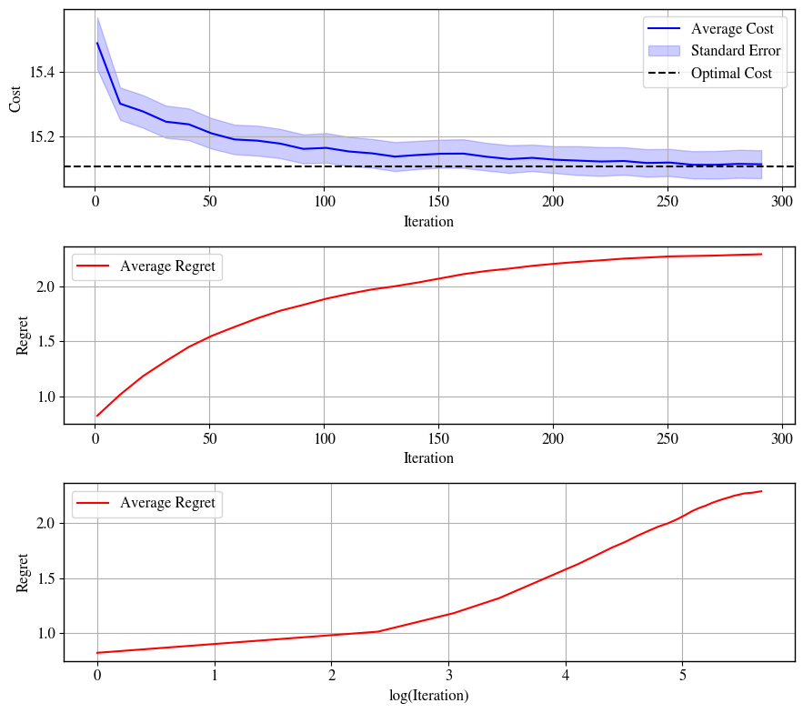
Our exploitation policy class $\Pi$ is given by neural networks with layer sizes $(4,64,64,64,1)$ and ReLU activation functions. For computational reasons, in place of directly solving for the certainty equivalent policy for each parameter estimate $\phi_{i}$, we simultaneously update a dynamics estimate $\phi_{i}$ and train our control parameters $\theta_{i}$ as follows. At each iteration, we update our estimate of $\phi_{i}$ as in Algorithm 1 to get a new estimate $\phi_{i+1}$; we then use the Adam optimizer (Kingma and Ba, 2014) to train a new set of control parameters $\theta_{i+1}$ to minimize the cost functions using trajectories sampled with the dynamics $\phi_{i+1}$ (in place of $\phi^{*}$), warm-starting the optimizer with the previous control parameters $\theta_{i}$. The initial exploration policy $\pi_{0}$ is given by bounded random noise scaled to match a predefined energy budget over the time horizon $T$; we choose a budget of $0.1T$. Finally, to illustrate the performance of our algorithm, we trained a ”best-in-class” controller $\pi^{*}$ using trajectories sampled with the true dynamics $\phi^{*}$.

In this experiment, we use the horizon $T=20$ and the number of episodes $N=300$. Finally, we note that in place of choosing the number of initial phase episodes $N_{\mathsf{phase\,1}}$, the confidence radius $r_{\Phi}$, and the step sizes $\eta_{i}$ according to Corollary 3.2 and Algorithm 1, we heuristically set $N_{\mathsf{phase\,1}}=1$, $r_{\Phi}=1$, and $\eta_{i}=100/(100+i)$. The cost of each controller was evaluated by sampling $10000$ trajectories and using the average cost; for computational reasons, we chose to only evaluate the cost every $10$ iterations.

Figure 2 illustrates the cost incurred by Algorithm 1 on the cartpole system. The first plot shows that the cost of the controllers chosen by Algorithm 1 converges to the cost of $\pi^{*}$ quickly, which in turn leads to sublinear regret as demonstrated in the second plot. We note that unlike the example in Section 4.1, the plot of regret versus logarithm of iteration does not show the same linear growth. This is due to two main reasons: first, we observed higher variance in estimating the costs of our cartpole controllers via sampling, leading to higher estimation error in both the average performance of Algorithm 1 as well as the optimal cost; second, due to the nonconvexity of optimizing neural network weights, our policy optimization steps were inexact, introducing additional discrepancies with our theory. However, the overall trend of fast convergence to the optimal control cost using a greedy algorithm is clear, and supports the behavior predicted by our theory. This cartpole experiment verifies that Algorithm 1 works on simple physical systems in practice.

References

• Boffi et al. (2021) Nicholas M Boffi, Stephen Tu, and Jean-Jacques E Slotine. Regret bounds for adaptive nonlinear control. In Learning for Dynamics and Control, pages 471–483. PMLR, 2021.
• Burnetas and Katehakis (1997) Apostolos N Burnetas and Michael N Katehakis. Optimal adaptive policies for markov decision processes. Mathematics of Operations Research, 22(1):222–255, 1997.
• Cassel et al. (2020) Asaf Cassel, Alon Cohen, and Tomer Koren. Logarithmic regret for learning linear quadratic regulators efficiently. In International Conference on Machine Learning, pages 1328–1337. PMLR, 2020.
• Charlet et al. (1989) B Charlet, J Levine, and R Marino. On dynamic feedback linearization. Systems & Control Letters, 13(2):143–151, 1989.
• Dann and Brunskill (2015) Christoph Dann and Emma Brunskill. Sample complexity of episodic fixed-horizon reinforcement learning. Advances in Neural Information Processing Systems, 28, 2015.
• Dean et al. (2020) Sarah Dean, Horia Mania, Nikolai Matni, Benjamin Recht, and Stephen Tu. On the sample complexity of the linear quadratic regulator. Foundations of Computational Mathematics, 20(4):633–679, 2020.
• Faradonbeh et al. (2018) Mohamad Kazem Shirani Faradonbeh, Ambuj Tewari, and George Michailidis. Finite time identification in unstable linear systems. Automatica, 96:342–353, 2018.
• Feldbaum (1960a) AA Feldbaum. Dual Control Theory. I. Avtomatika i Telemekhanika, 21(9):1240–1249, 1960a.
• Feldbaum (1960b) AA Feldbaum. Dual Control Theory. II. Avtomatika i Telemekhanika, 21(11):1453–1464, 1960b.
• Foster et al. (2020) Dylan Foster, Tuhin Sarkar, and Alexander Rakhlin. Learning nonlinear dynamical systems from a single trajectory. In Learning for Dynamics and Control, pages 851–861. PMLR, 2020.
• Garivier et al. (2019) Aurélien Garivier, Pierre Ménard, and Gilles Stoltz. Explore first, exploit next: The true shape of regret in bandit problems. Mathematics of Operations Research, 44(2):377–399, 2019.
• Jedra and Proutiere (2022) Yassir Jedra and Alexandre Proutiere. Minimal expected regret in linear quadratic control. In International Conference on Artificial Intelligence and Statistics, pages 10234–10321. PMLR, 2022.
• Jiang et al. (2017) Nan Jiang, Akshay Krishnamurthy, Alekh Agarwal, John Langford, and Robert E. Schapire. Contextual decision processes with low Bellman rank are PAC-learnable. In Doina Precup and Yee Whye Teh, editors, Proceedings of the 34th International Conference on Machine Learning, volume 70 of Proceedings of Machine Learning Research, pages 1704–1713. PMLR, 06–11 Aug 2017. URL https://proceedings.mlr.press/v70/jiang17c.html.
• Kakade et al. (2020) Sham Kakade, Akshay Krishnamurthy, Kendall Lowrey, Motoya Ohnishi, and Wen Sun. Information theoretic regret bounds for online nonlinear control. Advances in Neural Information Processing Systems, 33:15312–15325, 2020.
• Kingma and Ba (2014) Diederik P. Kingma and Jimmy Ba. Adam: A method for stochastic optimization. CoRR, abs/1412.6980, 2014. URL https://api.semanticscholar.org/CorpusID:6628106.
• Kober et al. (2013) Jens Kober, J Andrew Bagnell, and Jan Peters. Reinforcement learning in robotics: A survey. The International Journal of Robotics Research, 32(11):1238–1274, 2013.
• Lai (1986) Tze Leung Lai. Asymptotically efficient adaptive control in stochastic regression models. Advances in Applied Mathematics, 7(1):23–45, 1986.
• Lai and Robbins (1985) Tze Leung Lai and Herbert Robbins. Asymptotically efficient adaptive allocation rules. Advances in applied mathematics, 6(1):4–22, 1985.
• Lale et al. (2020) Sahin Lale, Kamyar Azizzadenesheli, Babak Hassibi, and Anima Anandkumar. Logarithmic regret bound in partially observable linear dynamical systems. Advances in Neural Information Processing Systems, 33:20876–20888, 2020.
• Lale et al. (2024) Sahin Lale, Peter I Renn, Kamyar Azizzadenesheli, Babak Hassibi, Morteza Gharib, and Anima Anandkumar. FALCON: Fourier adaptive learning and control for disturbance rejection under extreme turbulence. npj Robot, 2(1), September 2024.
• Lee et al. (2024a) Bruce Lee, Anders Rantzer, and Nikolai Matni. Nonasymptotic regret analysis of adaptive linear quadratic control with model misspecification. In 6th Annual Learning for Dynamics & Control Conference, pages 980–992. PMLR, 2024a.
• Lee et al. (2024b) Bruce D Lee, Ingvar Ziemann, George J Pappas, and Nikolai Matni. Active learning for control-oriented identification of nonlinear systems. arXiv preprint arXiv:2404.09030, 2024b.
• Lin et al. (1985) Woei Lin, PR Kumar, and TI Seidman. Will the self-tuning approach work for general cost criteria? Systems & control letters, 6(2):77–85, 1985.
• Ljung (1999) Lennart Ljung. System identification: theory for the user. PTR Prentice Hall, Upper Saddle River, NJ, 1999.
• Mania et al. (2022) Horia Mania, Michael I Jordan, and Benjamin Recht. Active learning for nonlinear system identification with guarantees. Journal of Machine Learning Research, 23(32):1–30, 2022.
• Ok et al. (2018) Jungseul Ok, Alexandre Proutiere, and Damianos Tranos. Exploration in structured reinforcement learning. Advances in Neural Information Processing Systems, 31, 2018.
• Ouyang et al. (2022) Long Ouyang, Jeffrey Wu, Xu Jiang, Diogo Almeida, Carroll Wainwright, Pamela Mishkin, Chong Zhang, Sandhini Agarwal, Katarina Slama, Alex Ray, et al. Training language models to follow instructions with human feedback. Advances in neural information processing systems, 35:27730–27744, 2022.
• Polderman (1986) Jan Willem Polderman. On the necessity of identifying the true parameter in adaptive lq control. Systems & control letters, 8(2):87–91, 1986.
• Robbins and Monro (1951) Herbert Robbins and Sutton Monro. A Stochastic Approximation Method. The Annals of Mathematical Statistics, 22(3):400 – 407, 1951. 10.1214/aoms/1177729586. URL https://doi.org/10.1214/aoms/1177729586.
• Roulet and d’Aspremont (2017) Vincent Roulet and Alexandre d’Aspremont. Sharpness, restart and acceleration. Advances in Neural Information Processing Systems, 30, 2017.
• Sattar and Oymak (2022) Yahya Sattar and Samet Oymak. Non-asymptotic and accurate learning of nonlinear dynamical systems. Journal of Machine Learning Research, 23(140):1–49, 2022.
• Silver et al. (2017) David Silver, Julian Schrittwieser, Karen Simonyan, Ioannis Antonoglou, Aja Huang, Arthur Guez, Thomas Hubert, Lucas Baker, Matthew Lai, Adrian Bolton, et al. Mastering the game of go without human knowledge. nature, 550(7676):354–359, 2017.
• Simchowitz and Foster (2020) Max Simchowitz and Dylan Foster. Naive exploration is optimal for online lqr. In International Conference on Machine Learning, pages 8937–8948. PMLR, 2020.
• Simchowitz et al. (2018) Max Simchowitz, Horia Mania, Stephen Tu, Michael I Jordan, and Benjamin Recht. Learning without mixing: Towards a sharp analysis of linear system identification. In Conference On Learning Theory, pages 439–473. PMLR, 2018.
• Treven et al. (2023) Lenart Treven, Cansu Sancaktar, Sebastian Blaes, Stelian Coros, and Andreas Krause. Optimistic active exploration of dynamical systems. Advances in Neural Information Processing Systems, 36:38122–38153, 2023.
• Wagenmaker et al. (2024) Andrew Wagenmaker, Guanya Shi, and Kevin G Jamieson. Optimal exploration for model-based rl in nonlinear systems. Advances in Neural Information Processing Systems, 36, 2024.
• Xu et al. (2021) Haike Xu, Tengyu Ma, and Simon Du. Fine-grained gap-dependent bounds for tabular mdps via adaptive multi-step bootstrap. In Conference on Learning Theory, pages 4438–4472. PMLR, 2021.
• Yang et al. (2020) Yuxiang Yang, Ken Caluwaerts, Atil Iscen, Tingnan Zhang, Jie Tan, and Vikas Sindhwani. Data efficient reinforcement learning for legged robots. In Conference on Robot Learning, pages 1–10. PMLR, 2020.
• Zhou et al. (2021) Dongruo Zhou, Quanquan Gu, and Csaba Szepesvari. Nearly minimax optimal reinforcement learning for linear mixture markov decision processes. In Conference on Learning Theory, pages 4532–4576. PMLR, 2021.
• Ziemann and Sandberg (2024) Ingvar Ziemann and Henrik Sandberg. Regret lower bounds for learning linear quadratic gaussian systems. IEEE Transactions on Automatic Control, 2024.
• Ziemann and Tu (2022) Ingvar Ziemann and Stephen Tu. Learning with little mixing. Advances in Neural Information Processing Systems, 35:4626–4637, 2022.
• Ziemann et al. (2024) Ingvar Ziemann, Stephen Tu, George J Pappas, and Nikolai Matni. Sharp rates in dependent learning theory: Avoiding sample size deflation for the square loss. In Forty-first International Conference on Machine Learning, 2024.
Appendix A Slow Learning
Here, we consider a more general setting where the assumption that the optimal policy has a positive definite Fisher Information (6) does not necessarily hold. In this setting, the approach of Section 3 fails, because the prediction error is no longer necessarily locally strongly convex near the optimal solution. Consequently, the result of the previous section no longer applies to achieve polylogarithmic regret. Instead, we propose an algorithm for which the learner incurs regret scaling with the square root of the number of interactions.
A.1 Additional Assumptions
To present the result for the setting where 6 does not necessarily hold, we strengthen the condition on the initial policy from that in 5 to the following.
Assumption 7
(Initial Lojasiewicz policy). Fix some positive constant CL​o​j​aC_{Loja}. The learner has access to a policy π0∈Π\pi_{0}\in\Pi which is (CL​o​j​a,1/2)(C_{Loja},1/2)-Lojasiewicz.
In particular, we restrict attention to settings where the Lojasiewicz condition holds with parameter 1/21/2. This means that estimation error grows quadratically with the parameter error. The assumption is made for ease of exposition. It would instead suffice to keep 5 and additionally assume that there exists a policy in the policy class which has a positive definite Fisher Information111Note that this is still substantially less restrictive than assuming that the optimal policy satisfies such a condition.. Then by using the optimal experiment design procedure of Lee et al. (2024b), one could find the policy with a positive definite Fisher information, which satisfies the Lojasiewicz condition with parameter α=1/2\alpha=1/2.
A.2 Algorithm and Regret Bound
Under Assumptions 1, 2, 3, 4, and 7, we give an algorithm with Regret⁡(N)=O​(N​log⁡N)\operatorname{Regret}(N)=O(\sqrt{N}\log N). This algorithm is based on an ”explore then commit” procedure in which the algorithm explores for some number of episodes to collect an initial dataset to synthesize a control policy π^\hat{\pi}, then plays π^\hat{\pi} for the remainder of the episodes.
Algorithm 2 Explore-Then-Commit
1:Initial policy π0\pi_{0}, policy class Π\Pi, number of episodes NN
2:Play π0\pi_{0} for N\sqrt{N} episodes to collect the dataset 𝒟←{(xt,ut,xt+1}t=1,n=1T,N\mathcal{D}\leftarrow\mathopen{}\left\{(x_{t},u_{t},x_{t+1}\right\}\mathclose{}_{t=1,n=1}^{T,\sqrt{N}}.
3: Set ϕ^\hat{\phi} as the least squares estimate (6) using the dataset 𝒟\mathcal{D}.
4:Set π^←π⋆​(ϕ^)\hat{\pi}\leftarrow\pi^{\star}(\hat{\phi}).
5:Play π^\hat{\pi} for the remaining N−NN-\sqrt{N} episodes.
Algorithm 2 is simpler than Algorithm 1, and just includes a single step of parameter estimation rather than continuously refining. We characterize the regret incurred by Algorithm 2 as follows.
Theorem A.1.
Consider applying Algorithm 2 to the system (1) with initial policy π0\pi_{0} satisfying 7, policy class Π\Pi satisfying 2 for NN episodes. Suppose that the dynamics satisfy 1 and that the costs satisfy 3. Furthermore, suppose that the dynamics, objective, and policy class satisfy 4. Then there exists polynomial function 𝗉𝗈𝗅𝗒𝖻𝗎𝗋𝗇​ ​𝗂𝗇\mathsf{poly}_{\mathsf{burn}\textnormal{ }\mathsf{in}} such that
𝔼\displaystyle\mathbb{E} [Regret(N)]≤𝗉𝗈𝗅𝗒(Lπ⋆,Lf,logB,Lθ,Lcost,σw,σw−1,T,dx,dϕ,logN)N.\displaystyle\mathopen{}\left[\operatorname{Regret}(N)\right]\mathclose{}\leq\mathsf{poly}\mathopen{}\left(L_{\pi^{\star}},L_{f},\log B,L_{\theta},L_{\operatorname{cost}},\sigma_{w},\sigma_{w}^{-1},T,d_{x},d_{\phi},\log N\right)\mathclose{}\sqrt{N}.
as long as N≥𝗉𝗈𝗅𝗒𝖻𝗎𝗋𝗇​𝗂𝗇(σw,dx,dϕ,logB,Lf,log(σw−1),logN,CLoja,rCE−1,rcost(ϕ⋆)−1)N\geq\mathsf{poly}_{\mathsf{burn\,in}}\mathopen{}\left(\sigma_{w},d_{x},d_{\phi},\log B,L_{f},\log(\sigma_{w}^{-1}),\log N,C_{\operatorname{Loja}},{r_{\operatorname{CE}}}^{-1},{r_{\operatorname{cost}}(\phi^{\star})}^{-1}\right)\mathclose{}.
This result follows by noting that the exploration phase incurs a regret proportional to the number of exploration episodes, N\sqrt{N}. For the exploitation phase, we leverage the smoothness of the cost functions, policy classes, and dynamics, to show that the excess cost incurred from a certainty equivalent policy scales quadratically with the estimation error ‖ϕ^−ϕ⋆‖\left\|\hat{\phi}-\phi_{\star}\right\|. Meanwhile, the system identification bounds of Lee et al. (2024b) demonstrate that the estimation error decays with 1/K1/\sqrt{K} when KK trajectories are used to fit ϕ^\hat{\phi} (neglecting system constants and log terms). By setting K=NK=\sqrt{N}, we find that ‖ϕ^−ϕ⋆‖\left\|\hat{\phi}-\phi_{\star}\right\| scales with 1/N1/41/N^{1/4}. Then the regret incurred in the exploration phase is N×‖ϕ^−ϕ⋆‖2​\lesssim​N×1N=NN\times\left\|\hat{\phi}-\phi_{\star}\right\|^{2}\lesssim N\times\frac{1}{\sqrt{N}}=\sqrt{N}, where \lesssim\lesssim hides logarithmic quantities and problem constants. Summing the regrets in the exploration phase with the exploitation phase then also results in a bound scaling with N\sqrt{N}. See Section A.3 for a rigorous proof.
A.3 Proof of Theorem A.1
To prove Theorem A.1 we first state two lemmas from Lee et al. (2024b)).
Lemma A.2 (Lemma A.1 of Lee et al. (2024b)).
Suppose Assumption 1 holds, and let δ∈(0,1/2]\delta\in(0,1/2]. Let ϕ^\hat{\phi} be the least squares estimate from (6) using KK episodes of data collected with a (CLoja,α)(C_{\operatorname{Loja}},\alpha) policy. There exists a polynomial function 𝗉𝗈𝗅𝗒α\mathsf{poly}_{\alpha} which depends on α\alpha such that with probability at least 1−δ1-\delta,
∥ϕ^−ϕ⋆∥2≤(512​σw2T​K(dx+dϕlog(4​B​Lf​T​Kσw​δ)))α.\displaystyle\left\|\hat{\phi}-\phi_{\star}\right\|^{2}\leq\left(\frac{512\sigma_{w}^{2}}{TK}\mathopen{}\left(d_{x}+d_{\phi}\log\mathopen{}\left(\frac{4BL_{f}TK}{\sigma_{w}\delta}\right)\mathclose{}\right)\mathclose{}\right)^{\alpha}.
as long as K≥τErr​(δ)=𝗉𝗈𝗅𝗒α​(σw,dx,dϕ,log⁡(B),Lf,CLoja,log⁡(K),log⁡1δ)K\geq\tau_{\operatorname{Err}}(\delta)=\mathsf{poly}_{\alpha}(\sigma_{w},d_{x},d_{\phi},\log(B),L_{f},C_{\operatorname{Loja}},\log(K),\log\frac{1}{\delta}).
Lemma A.3 (Modified from Lemma 3.1 of Lee et al. (2024b)).
Suppose Assumptions 1-4 hold. Then for ϕ^∈ℬ(ϕ⋆,min{rcost(ϕ⋆),rCE})\hat{\phi}\in\mathcal{B}(\phi^{\star},\min\mathopen{}\left\{r_{\operatorname{cost}}(\phi^{\star}),r_{\operatorname{CE}}\right\}\mathclose{}),
𝒥​(π⋆​(ϕ^),ϕ⋆)−𝒥​(π⋆​(ϕ⋆),ϕ⋆)≤Ccost​‖ϕ^−ϕ⋆‖2,\displaystyle\mathcal{J}(\pi^{\star}(\hat{\phi}),\phi^{\star})\!-\!\mathcal{J}(\pi^{\star}(\phi^{\star}),\phi^{\star})\!\leq C_{\operatorname{cost}}\!\left\|\hat{\phi}\!-\!\phi^{\star}\right\|^{2}, (13)
where Ccost=𝗉𝗈𝗅𝗒​(Lπ⋆,Lf,Lθ,Lcost,σw−1,T,dx)C_{\operatorname{cost}}=\mathsf{poly}(L_{\pi^{\star}},L_{f},L_{\theta},L_{\operatorname{cost}},\sigma_{w}^{-1},T,d_{x}).
Proof A.4.
The proof follows as in the proof of Lemma 3.1 of Lee et al. (2024b); however, the third order Taylor expansion is replaced with a second order expansion.
Armed with these results, we proceed to prove Theorem A.1. To begin, decompose the regret into the event conditioned on the success event of Lemma A.2 that holds with probability at least 1−1/N1-1/N, and the regret conditioned on the complement of that event. The condition to apply Lemma A.2 is satisfied due to the burn-in condition on NN. Denote the success event ℰ𝗌𝗎𝖼𝖼𝖾𝗌𝗌\mathcal{E}_{\mathsf{success}}. It holds that
𝔼[Regret(N)]\displaystyle\mathbb{E}\mathopen{}\left[\operatorname{Regret}(N)\right]\mathclose{} =ℙ(ℰ𝗌𝗎𝖼𝖼𝖾𝗌𝗌)𝔼[Regret(N)∣ℰ𝗌𝗎𝖼𝖼𝖾𝗌𝗌]+(1−ℰ𝗌𝗎𝖼𝖼𝖾𝗌𝗌)𝔼[Regret(N)∣ℰ𝗌𝗎𝖼𝖼𝖾𝗌𝗌c]\displaystyle=\mathbb{P}(\mathcal{E}_{\mathsf{success}})\mathbb{E}\mathopen{}\left[\operatorname{Regret}(N)\mid\mathcal{E}_{\mathsf{success}}\right]\mathclose{}+(1-\mathcal{E}_{\mathsf{success}})\mathbb{E}\mathopen{}\left[\operatorname{Regret}(N)\mid\mathcal{E}_{\mathsf{success}}^{c}\right]\mathclose{}
≤𝔼[Regret(N)∣ℰ𝗌𝗎𝖼𝖼𝖾𝗌𝗌]+(1/N)NLcost\displaystyle\leq\mathbb{E}\mathopen{}\left[\operatorname{Regret}(N)\mid\mathcal{E}_{\mathsf{success}}\right]\mathclose{}+(1/N)NL_{\operatorname{cost}}
=𝔼[∑n=1N(J(πn,ϕ∗)−minπ∈ΠJ(π,ϕ∗))∣ℰ𝗌𝗎𝖼𝖼𝖾𝗌𝗌]+Lcost,\displaystyle=\mathbb{E}\mathopen{}\left[\sum_{n=1}^{N}{(J(\pi_{n},\phi^{*})-\min_{\pi\in\Pi}{J(\pi,\phi^{*}))}}\mid\mathcal{E}_{\mathsf{success}}\right]\mathclose{}+L_{\operatorname{cost}},
where the inequality follows from the probability bound on the failure event, and the fact that the cost incurred during each episode is bounded by LcostL_{\operatorname{cost}}. We may further decompose the cost into the cost incurred during the exploration phase (episodes 11 to N\sqrt{N}) and the cost incurred in the exploitation phase N\sqrt{N} to NN. Leveraging the fact that the costs are bounded, we may therefore bound the cost incurred during the exploration phase by N​Lcost\sqrt{N}L_{\operatorname{cost}}:
𝔼[Regret(N)]\displaystyle\mathbb{E}\mathopen{}\left[\operatorname{Regret}(N)\right]\mathclose{} ≤Lcost+𝔼[∑n=1N(J(π0,ϕ∗)−minπ∈ΠJ(π,ϕ∗))∣ℰ𝗌𝗎𝖼𝖼𝖾𝗌𝗌]\displaystyle\leq L_{\operatorname{cost}}+\mathbb{E}\mathopen{}\left[\sum_{n=1}^{\sqrt{N}}{(J(\pi_{0},\phi^{*})-\min_{\pi\in\Pi}{J(\pi,\phi^{*}))}}\mid\mathcal{E}_{\mathsf{success}}\right]\mathclose{}
+𝔼[∑n=N+1N(J(π⋆(ϕ^),ϕ∗)−minπ∈ΠJ(π,ϕ∗))∣ℰ𝗌𝗎𝖼𝖼𝖾𝗌𝗌]\displaystyle\qquad+\mathbb{E}\mathopen{}\left[\sum_{n=\sqrt{N}+1}^{N}{(J(\pi^{\star}(\hat{\phi}),\phi^{*})-\min_{\pi\in\Pi}{J(\pi,\phi^{*}))}}\mid\mathcal{E}_{\mathsf{success}}\right]\mathclose{}
=Lcost+N𝔼[(J(π0,ϕ∗)−minπ∈ΠJ(π,ϕ∗))∣ℰ𝗌𝗎𝖼𝖼𝖾𝗌𝗌]\displaystyle=L_{\operatorname{cost}}+\sqrt{N}\mathbb{E}\mathopen{}\left[{(J(\pi_{0},\phi^{*})-\min_{\pi\in\Pi}{J(\pi,\phi^{*}))}}\mid\mathcal{E}_{\mathsf{success}}\right]\mathclose{}
+(N−N)𝔼[(J(π⋆(ϕ^),ϕ∗)−minπ∈ΠJ(π,ϕ∗))∣ℰ𝗌𝗎𝖼𝖼𝖾𝗌𝗌]\displaystyle\qquad+(N-\sqrt{N})\mathbb{E}\mathopen{}\left[{(J(\pi^{\star}(\hat{\phi}),\phi^{*})-\min_{\pi\in\Pi}{J(\pi,\phi^{*}))}}\mid\mathcal{E}_{\mathsf{success}}\right]\mathclose{}
≤Lcost+NLcost+N𝔼[(J(π⋆(ϕ^),ϕ∗)−minπ∈ΠJ(π,ϕ∗))∣ℰ𝗌𝗎𝖼𝖼𝖾𝗌𝗌].\displaystyle\leq L_{\operatorname{cost}}+\sqrt{N}L_{\operatorname{cost}}+N\mathbb{E}\mathopen{}\left[{(J(\pi^{\star}(\hat{\phi}),\phi^{*})-\min_{\pi\in\Pi}{J(\pi,\phi^{*}))}}\mid\mathcal{E}_{\mathsf{success}}\right]\mathclose{}.
where ϕ^\hat{\phi} is the parameter estimate from 3 of Algorithm 2. To continue the proof, we need to bound the term:
N​𝔼​[J​(π⋆​(ϕ^),ϕ∗)−minπ∈Π⁡J​(π,ϕ∗)∣ℰ𝗌𝗎𝖼𝖼𝖾𝗌𝗌],N\mathbb{E}\left[J(\pi^{\star}(\hat{\phi}),\phi^{*})-\min_{\pi\in\Pi}J(\pi,\phi^{*})\mid\mathcal{E}_{\mathsf{success}}\right],
where ℰ𝗌𝗎𝖼𝖼𝖾𝗌𝗌\mathcal{E}_{\mathsf{success}} denotes the event where the estimation error ‖ϕ^−ϕ∗‖\|\hat{\phi}-\phi^{*}\| is small, as guaranteed by Lemma A.2. Under the event ℰ𝗌𝗎𝖼𝖼𝖾𝗌𝗌\mathcal{E}_{\mathsf{success}}, from Lemma A.2, it holds that
‖ϕ^−ϕ∗‖2≤512​σw2T​N​(dx+dϕ​log⁡(4​B​Lf​T​Nσw​δ))≤C𝗂𝖽𝖾𝗇𝗍𝗂𝖿𝗂𝖼𝖺𝗍𝗂𝗈𝗇N,\|\hat{\phi}-\phi^{*}\|^{2}\leq\frac{512\sigma_{w}^{2}}{T\sqrt{N}}\left(d_{x}+d_{\phi}\log\left(\frac{4BL_{f}T\sqrt{N}}{\sigma_{w}\delta}\right)\right)\leq\frac{C_{\mathsf{identification}}}{\sqrt{N}},
where C𝗂𝖽𝖾𝗇𝗍𝗂𝖿𝗂𝖼𝖺𝗍𝗂𝗈𝗇:=𝗉𝗈𝗅𝗒​(σw,dx,dϕ,log⁡(B),log⁡(Lf),log⁡(T),log⁡(N))C_{\mathsf{identification}}:=\mathsf{poly}(\sigma_{w},d_{x},d_{\phi},\log(B),\log(L_{f}),\log(T),\log(N)). From Lemma A.3, it holds that for ϕ^\hat{\phi} within a neighborhood of ϕ∗\phi^{*},
J​(π⋆​(ϕ^),ϕ∗)−J​(π⋆​(ϕ∗),ϕ∗)\displaystyle J(\pi^{\star}(\hat{\phi}),\phi^{*})-J(\pi^{\star}(\phi^{*}),\phi^{*}) ≤Ccost​‖ϕ^−ϕ∗‖2.\displaystyle\leq C_{\operatorname{cost}}\|\hat{\phi}-\phi^{*}\|^{2}.
In particular, it suffices to use the bound on ‖ϕ^−ϕ⋆‖\left\|\hat{\phi}-\phi^{\star}\right\| along with the burn-in condition on NN to ensure that ‖ϕ^−ϕ⋆‖\left\|\hat{\phi}-\phi^{\star}\right\| is small enough to instantiate Lemma A.3. Substituting this bound into the overall regret bound, it holds that
𝔼​[Regret⁡(N)]\displaystyle\mathbb{E}\left[\operatorname{Regret}(N)\right] ≤Lcost​(1+N)+N​𝔼​[J​(π⋆​(ϕ^),ϕ∗)−J​(π⋆​(ϕ∗),ϕ∗)∣ℰ𝗌𝗎𝖼𝖼𝖾𝗌𝗌]\displaystyle\leq L_{\operatorname{cost}}(1+\sqrt{N})+N\mathbb{E}\left[J(\pi^{\star}(\hat{\phi}),\phi^{*})-J(\pi^{\star}(\phi^{*}),\phi^{*})\mid\mathcal{E}_{\mathsf{success}}\right]
≤Lcost​(1+N)+C𝗂𝖽𝖾𝗇𝗍𝗂𝖿𝗂𝖼𝖺𝗍𝗂𝗈𝗇​Ccost​N.\displaystyle\leq L_{\operatorname{cost}}(1+\sqrt{N})+C_{\mathsf{identification}}C_{\operatorname{cost}}\sqrt{N}.
Thus, we conclude:
𝔼​[Regret⁡(N)]≤𝗉𝗈𝗅𝗒​(Lπ⋆,Lf,log⁡(B),Lθ,Lcost,σw,σw−1,T,dx,dϕ,log⁡(N))​N.\mathbb{E}\left[\operatorname{Regret}(N)\right]\leq\mathsf{poly}(L_{\pi^{\star}},L_{f},\log(B),L_{\theta},L_{\operatorname{cost}},\sigma_{w},\sigma_{w}^{-1},T,d_{x},d_{\phi},\log(N))\sqrt{N}.
Appendix B Proofs for Fast Learning
B.1 Results for Persistently Exciting Systems
Before proving Theorem 3.1, we state and prove some useful results for systems for which the optimal controller is persistently exciting.
The following results show that if the optimal controller πθ∗​(ϕ∗)\pi_{\theta^{*}(\phi^{*})} is persistently exciting (Assumption 6), then all controllers πθ\pi_{\theta}, where θ\theta is in an open ball centered around θ∗\theta^{*}, are also persistently exciting.
Lemma B.1.
Suppose that Assumptions 1 and 2 hold. Then for all θ∈ℝdθ\theta\in\mathbb{R}^{d_{\theta}},
∥Dθ(DΦ(2)Errπθϕ∗(ϕ∗))|θ=θ∥op≤2TLf2Lθ+T2​Lf3​Lθ​dxσw.\displaystyle\left\|D_{\theta}\mathopen{}\left(D_{\Phi}^{(2)}\operatorname{Err}_{\pi_{\theta}}^{\phi^{*}}(\phi^{*})\right)\mathclose{}\bigg{\rvert}_{\theta=\theta}\right\|_{\operatorname{op}}\leq 2TL_{f}^{2}L_{\theta}+\frac{T^{2}L_{f}^{3}L_{\theta}\sqrt{d_{x}}}{\sigma_{w}}.
Proof B.2.
Since the dynamics are rolled out under πθ\pi_{\theta}, we have:
Dθ(DΦ(2)Errπθϕ∗(ϕ∗))|θ=θ=Dθ(𝔼πθϕ∗[∑t=1TDf(xt,πθ(xt),ϕ∗)⊤Df(xt,πθ(xt),ϕ∗)])|θ=θ=Dθ(∫(∑t=1TDf(xt,πθ(xt),ϕ∗)⊤Df(xt,πθ(xt),ϕ∗))pπθϕ∗(x1:T+1)d(x1:T+1))|θ=θD_{\theta}\mathopen{}\left(D_{\Phi}^{(2)}\operatorname{Err}_{\pi_{\theta}}^{\phi^{*}}(\phi^{*})\right)\mathclose{}\bigg{\rvert}_{\theta=\theta}=D_{\theta}\mathopen{}\left(\mathbb{E}^{\phi^{*}}_{\pi_{\theta}}\mathopen{}\left[\sum_{t=1}^{T}{Df(x_{t},\pi_{\theta}(x_{t}),\phi^{*})^{\top}Df(x_{t},\pi_{\theta}(x_{t}),\phi^{*})}\right]\mathclose{}\right)\mathclose{}\bigg{\rvert}_{\theta=\theta}\\ =D_{\theta}\mathopen{}\left(\int{\mathopen{}\left(\sum_{t=1}^{T}{Df(x_{t},\pi_{\theta}(x_{t}),\phi^{*})^{\top}Df(x_{t},\pi_{\theta}(x_{t}),\phi^{*})}\right)\mathclose{}\>p_{\pi_{\theta}}^{\phi^{*}}(x_{1:T+1})d(x_{1:T+1)}}\right)\mathclose{}\bigg{\rvert}_{\theta=\theta} (14)
Here pπθϕ∗​(x1:T+1)p_{\pi_{\theta}}^{\phi^{*}}(x_{1:T+1}) is the density of the trajectory x1:T+1x_{1:T+1} under dynamics ϕ\phi* and controller πθ\pi_{\theta} and can be written as:
pπθϕ∗(x1:T+1)=(1σw​2​π)Texp(−12​σw2∑t=1T∥f(xt,πθ(xt),ϕ∗)−xt+1∥2)\displaystyle p_{\pi_{\theta}}^{\phi^{*}}(x_{1:T+1})=\mathopen{}\left(\frac{1}{\sigma_{w}\sqrt{2\pi}}\right)\mathclose{}^{T}\exp\mathopen{}\left(-\frac{1}{2\sigma_{w}^{2}}\sum_{t=1}^{T}{\|f(x_{t},\pi_{\theta}(x_{t}),\phi^{*})-x_{t+1}\|^{2}}\right)\mathclose{} (15)
By the dominated convergence theorem, followed by the product rule, we may rewrite (14) as:
Dθ(DΦ(2)Errπθϕ∗(ϕ∗))|θ=θ=∫(Dθ((∑t=1TDf(xt,πθ(xt),ϕ∗)⊤Df(xt,πθ(xt),ϕ∗))pπθϕ∗(x1:T+1))|θ=θ)d(x1:T+1)=∫(Dθ(∑t=1TDf(xt,πθ(xt),ϕ∗)⊤Df(xt,πθ(xt),ϕ∗))|θ=θ)pπθϕ∗(x1:T+1)d(x1:T+1)+∫(∑t=1TDf(xt,πθ(xt),ϕ∗)⊤Df(xt,πθ(xt),ϕ∗))(Dθ(pπθϕ∗(x1:T+1)I)|θ=θ)d(x1:T+1)D_{\theta}\mathopen{}\left(D_{\Phi}^{(2)}\operatorname{Err}_{\pi_{\theta}}^{\phi^{*}}(\phi^{*})\right)\mathclose{}\bigg{\rvert}_{\theta=\theta}=\int{\mathopen{}\left(D_{\theta}\mathopen{}\left(\mathopen{}\left(\sum_{t=1}^{T}{Df(x_{t},\pi_{\theta}(x_{t}),\phi^{*})^{\top}Df(x_{t},\pi_{\theta}(x_{t}),\phi^{*})}\right)\mathclose{}p_{\pi_{\theta}}^{\phi^{*}}(x_{1:T+1})\right)\mathclose{}\bigg{\rvert}_{\theta=\theta}\right)\mathclose{}\>d(x_{1:T+1)}}=\int{\mathopen{}\left(D_{\theta}\mathopen{}\left(\sum_{t=1}^{T}{Df(x_{t},\pi_{\theta}(x_{t}),\phi^{*})^{\top}Df(x_{t},\pi_{\theta}(x_{t}),\phi^{*})}\right)\mathclose{}\bigg{\rvert}_{\theta=\theta}\right)\mathclose{}\>p_{\pi_{\theta}}^{\phi^{*}}(x_{1:T+1})d(x_{1:T+1})}+\int{\mathopen{}\left(\sum_{t=1}^{T}{Df(x_{t},\pi_{\theta}(x_{t}),\phi^{*})^{\top}Df(x_{t},\pi_{\theta}(x_{t}),\phi^{*})}\right)\mathclose{}\mathopen{}\left(D_{\theta}\mathopen{}\left(p_{\pi_{\theta}}^{\phi^{*}}(x_{1:T+1})I\right)\mathclose{}\bigg{\rvert}_{\theta=\theta}\right)\mathclose{}\>d(x_{1:T+1})} (16)
We proceed by bounding the operator norms of the two integrals in equation (16). To bound the operator norm of the first integral, we apply Jensen’s inequality followed by Assumptions 1 and 2:
∥∫(Dθ(∑t=1TDf(xt,πθ(xt),ϕ∗)⊤Df(xt,πθ(xt),ϕ∗))|θ=θ)pπθϕ∗(x1:T+1)d(x1:T+1)∥op≤∫∥(Dθ(∑t=1TDf(xt,πθ(xt),ϕ∗)⊤Df(xt,πθ(xt),ϕ∗))|θ=θ)∥oppπθϕ∗(x1:T+1)d(x1:T+1)≤2TLf2Lθ\left\|\int{\mathopen{}\left(D_{\theta}\mathopen{}\left(\sum_{t=1}^{T}{Df(x_{t},\pi_{\theta}(x_{t}),\phi^{*})^{\top}Df(x_{t},\pi_{\theta}(x_{t}),\phi^{*})}\right)\mathclose{}\bigg{\rvert}_{\theta=\theta}\right)\mathclose{}\>p_{\pi_{\theta}}^{\phi^{*}}(x_{1:T+1})d(x_{1:T+1})}\right\|_{\operatorname{op}}\\ \leq\int{\left\|\mathopen{}\left(D_{\theta}\mathopen{}\left(\sum_{t=1}^{T}{Df(x_{t},\pi_{\theta}(x_{t}),\phi^{*})^{\top}Df(x_{t},\pi_{\theta}(x_{t}),\phi^{*})}\right)\mathclose{}\bigg{\rvert}_{\theta=\theta}\right)\mathclose{}\right\|_{\operatorname{op}}\>p_{\pi_{\theta}}^{\phi^{*}}(x_{1:T+1})d(x_{1:T+1})}\\ \leq 2TL_{f}^{2}L_{\theta} (17)
To bound the operator norm of the second integral, we first apply Jensen’s inequality, followed by the submultiplicative property of operator norm, followed by the identity ∇g​(x)=g​(x)​∇log⁡g​(x)\nabla g(x)=g(x)\nabla\log g(x) for g:ℝn→ℝg:\mathbb{R}^{n}\to\mathbb{R}:
∥∫(∑t=1TDf(xt,πθ(xt),ϕ∗)⊤Df(xt,πθ(xt),ϕ∗))(Dθ(pπθϕ∗(x1:T+1)I)|θ=θ)d(x1:T+1)∥op≤∫∥∑t=1TDf(xt,πθ(xt),ϕ∗)⊤Df(xt,πθ(xt),ϕ∗)∥op∥Dθ(pπθϕ∗(x1:T+1)I)|θ=θ∥opd(x1:T+1)=∫∥∑t=1TDf(xt,πθ(xt),ϕ∗)⊤Df(xt,πθ(xt),ϕ∗)∥op∥∇θ(pπθϕ∗(x1:T+1))|θ=θ∥d(x1:T+1)=∫∥∑t=1TDf(xt,πθ(xt),ϕ∗)⊤Df(xt,πθ(xt),ϕ∗)∥op∥∇θ(logpπθϕ∗(x1:T+1))|θ=θ∥pπθϕ∗(x1:T+1)d(x1:T+1)≤TLf2∫∥∇θ(logpπθϕ∗(x1:T+1))|θ=θ∥pπθϕ∗(x1:T+1)d(x1:T+1)\left\|\int{\mathopen{}\left(\sum_{t=1}^{T}{Df(x_{t},\pi_{\theta}(x_{t}),\phi^{*})^{\top}Df(x_{t},\pi_{\theta}(x_{t}),\phi^{*})}\right)\mathclose{}\mathopen{}\left(D_{\theta}\mathopen{}\left(p_{\pi_{\theta}}^{\phi^{*}}(x_{1:T+1})I\right)\mathclose{}\bigg{\rvert}_{\theta=\theta}\right)\mathclose{}\>d(x_{1:T+1})}\right\|_{\operatorname{op}}\\ \leq\int{\left\|\sum_{t=1}^{T}{Df(x_{t},\pi_{\theta}(x_{t}),\phi^{*})^{\top}Df(x_{t},\pi_{\theta}(x_{t}),\phi^{*})}\right\|_{\operatorname{op}}\left\|D_{\theta}\mathopen{}\left(p_{\pi_{\theta}}^{\phi^{*}}(x_{1:T+1})I\right)\mathclose{}\bigg{\rvert}_{\theta=\theta}\right\|_{\operatorname{op}}\>d(x_{1:T+1})}\\ =\int{\left\|\sum_{t=1}^{T}{Df(x_{t},\pi_{\theta}(x_{t}),\phi^{*})^{\top}Df(x_{t},\pi_{\theta}(x_{t}),\phi^{*})}\right\|_{\operatorname{op}}\left\|\nabla_{\theta}\mathopen{}\left(p_{\pi_{\theta}}^{\phi^{*}}(x_{1:T+1})\right)\mathclose{}\bigg{\rvert}_{\theta=\theta}\right\|\>d(x_{1:T+1})}\\ =\int{\left\|\sum_{t=1}^{T}{Df(x_{t},\pi_{\theta}(x_{t}),\phi^{*})^{\top}Df(x_{t},\pi_{\theta}(x_{t}),\phi^{*})}\right\|_{\operatorname{op}}\left\|\nabla_{\theta}\mathopen{}\left(\log p_{\pi_{\theta}}^{\phi^{*}}(x_{1:T+1})\right)\mathclose{}\bigg{\rvert}_{\theta=\theta}\right\|\>p_{\pi_{\theta}}^{\phi^{*}}(x_{1:T+1})d(x_{1:T+1})}\\ \leq TL_{f}^{2}\int{\left\|\nabla_{\theta}\mathopen{}\left(\log p_{\pi_{\theta}}^{\phi^{*}}(x_{1:T+1})\right)\mathclose{}\bigg{\rvert}_{\theta=\theta}\right\|\>p_{\pi_{\theta}}^{\phi^{*}}(x_{1:T+1})d(x_{1:T+1})} (18)
Then, we substitute (15) for the density pπθϕ∗​(x1:T+1)p_{\pi_{\theta}}^{\phi^{*}}(x_{1:T+1}), then apply the triangular inequality, followed by Assumptions 1 and 2:
TLf2∫∥∇θ(logpπθϕ∗(x1:T+1))|θ=θ∥pπθϕ∗(x1:T+1)d(x1:T+1)=TLf2∫∥∇θ(log((1σw​2​π)Texp(−12​σw2∑t=1T∥f(xt,πθ(xt),ϕ∗)−xt+1∥2)))|θ=θ∥pπθϕ∗(x1:T+1)d(x1:T+1)=T​Lf22​σw2∫∥∇θ(∑t=1T∥f(xt,πθ(xt),ϕ∗)−xt+1∥2)|θ=θ∥pπθϕ∗(x1:T+1)d(x1:T+1)=T​Lf2σw2∫∥∑t=1T(f(xt,πθ(xt),ϕ∗)−xt+1)⊤(Duf(xt,πθ(xt),ϕ∗))(Dθπθ(xt)|θ=θ)∥pπθϕ∗(x1:T+1)d(x1:T+1)≤T​Lf3​Lθσw2∫(∑t=1T∥f(xt,πθ(xt),ϕ∗)−xt+1∥)pπθϕ∗(x1:T+1)d(x1:T+1)TL_{f}^{2}\int{\left\|\nabla_{\theta}\mathopen{}\left(\log p_{\pi_{\theta}}^{\phi^{*}}(x_{1:T+1})\right)\mathclose{}\bigg{\rvert}_{\theta=\theta}\right\|\>p_{\pi_{\theta}}^{\phi^{*}}(x_{1:T+1})d(x_{1:T+1})}=TL_{f}^{2}\int{\left\|\nabla_{\theta}\mathopen{}\left(\log\mathopen{}\left(\mathopen{}\left(\frac{1}{\sigma_{w}\sqrt{2\pi}}\right)\mathclose{}^{T}\exp\mathopen{}\left(-\frac{1}{2\sigma_{w}^{2}}\sum_{t=1}^{T}{\|f(x_{t},\pi_{\theta}(x_{t}),\phi^{*})-x_{t+1}\|^{2}}\right)\mathclose{}\right)\mathclose{}\right)\mathclose{}\bigg{\rvert}_{\theta=\theta}\right\|\>p_{\pi_{\theta}}^{\phi^{*}}(x_{1:T+1})d(x_{1:T+1})}\\ =\frac{TL_{f}^{2}}{2\sigma_{w}^{2}}\int{\left\|\nabla_{\theta}\mathopen{}\left(\sum_{t=1}^{T}{\|f(x_{t},\pi_{\theta}(x_{t}),\phi^{*})-x_{t+1}\|^{2}}\right)\mathclose{}\bigg{\rvert}_{\theta=\theta}\right\|\>p_{\pi_{\theta}}^{\phi^{*}}(x_{1:T+1})d(x_{1:T+1})}\\ =\frac{TL_{f}^{2}}{\sigma_{w}^{2}}\int{\left\|\sum_{t=1}^{T}{\mathopen{}\left(f(x_{t},\pi_{\theta}(x_{t}),\phi^{*})-x_{t+1}\right)\mathclose{}^{\top}\mathopen{}\left(D_{u}f(x_{t},\pi_{\theta}(x_{t}),\phi^{*})\right)\mathclose{}\mathopen{}\left(D_{\theta}\pi_{\theta}(x_{t})\rvert_{\theta=\theta}\right)\mathclose{}}\right\|\>p_{\pi_{\theta}}^{\phi^{*}}(x_{1:T+1})d(x_{1:T+1})}\\ \leq\frac{TL_{f}^{3}L_{\theta}}{\sigma_{w}^{2}}\int{\mathopen{}\left(\sum_{t=1}^{T}{\left\|f(x_{t},\pi_{\theta}(x_{t}),\phi^{*})-x_{t+1}\right\|}\right)\mathclose{}\>p_{\pi_{\theta}}^{\phi^{*}}(x_{1:T+1})d(x_{1:T+1})} (19)
We can bound the remaining integral with the expected norm of a Gaussian random vector Y∼𝒩​(0,σw2​I)Y\sim\mathcal{N}(0,\sigma^{2}_{w}I):
T​Lf3​Lθσw2∫(∑t=1T∥f(xt,πθ(xt),ϕ∗)−xt+1∥)pπθϕ∗(x1:T+1)d(x1:T+1)≤T2​Lf3​Lθ​dxσw\frac{TL_{f}^{3}L_{\theta}}{\sigma_{w}^{2}}\int{\mathopen{}\left(\sum_{t=1}^{T}{\left\|f(x_{t},\pi_{\theta}(x_{t}),\phi^{*})-x_{t+1}\right\|}\right)\mathclose{}\>p_{\pi_{\theta}}^{\phi^{*}}(x_{1:T+1})d(x_{1:T+1})}\leq\frac{T^{2}L_{f}^{3}L_{\theta}\sqrt{d_{x}}}{\sigma_{w}} (20)
Combining our bounds for the first and second integrals in (16), we conclude:
∥Dθ(DΦ(2)Errπθϕ∗(ϕ∗))|θ=θ∥op≤2TLf2Lθ+T2​Lf3​Lθ​dxσw\left\|D_{\theta}\mathopen{}\left(D_{\Phi}^{(2)}\operatorname{Err}_{\pi_{\theta}}^{\phi^{*}}(\phi^{*})\right)\mathclose{}\bigg{\rvert}_{\theta=\theta}\right\|_{\operatorname{op}}\leq 2TL_{f}^{2}L_{\theta}+\frac{T^{2}L_{f}^{3}L_{\theta}\sqrt{d_{x}}}{\sigma_{w}} (21)
The following results demonstrate that, for any persistent exciting controller π\pi, the prediction error of dynamics ϕ\phi (using trajectories collected with controller π\pi) is locally strongly convex near the true dynamics ϕ∗\phi^{*}. These results allow us to analyze the second phase of our algorithm through the lens of online convex optimization.
Lemma B.3.
Assume that Assumption 1 holds. Then for any controller π\pi, and all ϕ∈ℝdΦ\phi\in\mathbb{R}^{d_{\Phi}},
‖DΦ(3)​Errπϕ∗⁡(ϕ)‖op≤6​T​Lf2+2​T​Lf2​‖ϕ−ϕ∗‖+2​T​Lf​σw​dx.\displaystyle\left\|D_{\Phi}^{(3)}\operatorname{Err}_{\pi}^{\phi^{*}}(\phi)\right\|_{\operatorname{op}}\leq 6TL_{f}^{2}+2TL_{f}^{2}\left\|\phi-\phi^{*}\right\|+2TL_{f}\sigma_{w}\sqrt{d_{x}}.
Proof B.4.
By the dominated convergence theorem followed by the product rule, the second derivative of the prediction error for dynamics ϕ\phi under controller π\pi, evaluated at ϕ\phi, is:
DΦ(2)(𝔼πϕ∗[∑t=1T∥f(xt,ut,ϕ)−xt+1∥2])|ϕ=ϕ=DΦ(2)(∫(∑t=1T∥f(xt,ut,ϕ)−xt+1∥2)pπ,ϕ∗(x1:T+1)d(x1:T+1))|ϕ=ϕ=∫(DΦ(2)(∑t=1T∥f(xt,ut,ϕ)−xt+1∥2)|ϕ=ϕ)pπ,ϕ∗(x1:T+1)d(x1:T+1)=∫(∑t=1T(2DΦf(xt,ut,ϕ)⊤DΦf(xt,ut,ϕ)+2(f(xt,ut,ϕ)−xt+1)⊤DΦ(2)f(xt,ut,ϕ)))pπ,ϕ∗(x1:T+1)d(x1:T+1)D^{(2)}_{\Phi}\mathopen{}\left(\mathbb{E}_{\pi}^{\phi^{*}}\mathopen{}\left[\sum_{t=1}^{T}{\left\|f(x_{t},u_{t},\phi)-x_{t+1}\right\|^{2}}\right]\mathclose{}\right)\mathclose{}\bigg{\rvert}_{\phi=\phi}=D^{(2)}_{\Phi}\mathopen{}\left(\int{\mathopen{}\left(\sum_{t=1}^{T}{\left\|f(x_{t},u_{t},\phi)-x_{t+1}\right\|^{2}}\right)\mathclose{}\>p_{\pi,\phi^{*}}(x_{1:T+1})d(x_{1:T+1})}\right)\mathclose{}\bigg{\rvert}_{\phi=\phi}=\int{\mathopen{}\left(D_{\Phi}^{(2)}\mathopen{}\left(\sum_{t=1}^{T}{\left\|f(x_{t},u_{t},\phi)-x_{t+1}\right\|^{2}}\right)\mathclose{}\bigg{\rvert}_{\phi=\phi}\right)\mathclose{}\>p_{\pi,\phi^{*}}(x_{1:T+1})d(x_{1:T+1})}=\int\Bigg{(}\sum_{t=1}^{T}\mathopen{}\left(2D_{\Phi}f(x_{t},u_{t},\phi)^{\top}D_{\Phi}f(x_{t},u_{t},\phi)\\ +2(f(x_{t},u_{t},\phi)-x_{t+1})^{\top}D_{\Phi}^{(2)}f(x_{t},u_{t},\phi)\right)\mathclose{}\Bigg{)}\>p_{\pi,\phi^{*}}(x_{1:T+1})d(x_{1:T+1}) (22)
Differentiating this once more with respect to ϕ\phi, we find:
DΦ(3)(𝔼πϕ∗[∑t=1T∥f(xt,ut,ϕ)−xt+1∥2])|ϕ=ϕ=DΦ(∫(∑t=1T(2DΦf(xt,ut,ϕ)⊤DΦf(xt,ut,ϕ)+2(f(xt,ut,ϕ)−xt+1)⊤DΦ(2)f(xt,ut,ϕ)))pπ,ϕ∗(x1:T+1)d(x1:T+1))|ϕ=ϕ=∫(∑t=1T(6DΦf(xt,ut,ϕ)⊤DΦ(2)f(xt,ut,ϕ)+2(f(xt,ut,ϕ)−xt+1)⊤DΦ(3)f(xt,ut,ϕ))pπ,ϕ∗(x1:T+1)d(x1:T+1)D^{(3)}_{\Phi}\mathopen{}\left(\mathbb{E}_{\pi}^{\phi^{*}}\mathopen{}\left[\sum_{t=1}^{T}{\left\|f(x_{t},u_{t},\phi)-x_{t+1}\right\|^{2}}\right]\mathclose{}\right)\mathclose{}\bigg{\rvert}_{\phi=\phi}=D_{\Phi}\Bigg{(}\int\Bigg{(}\sum_{t=1}^{T}\mathopen{}\left(2D_{\Phi}f(x_{t},u_{t},\phi)^{\top}D_{\Phi}f(x_{t},u_{t},\phi)\\ +2(f(x_{t},u_{t},\phi)-x_{t+1})^{\top}D_{\Phi}^{(2)}f(x_{t},u_{t},\phi)\right)\mathclose{}\Bigg{)}\>p_{\pi,\phi^{*}}(x_{1:T+1})d(x_{1:T+1})\Bigg{)}\bigg{\rvert}_{\phi=\phi}=\int\mathopen{}\left(\sum_{t=1}^{T}\mathopen{}\left(6D_{\Phi}f(x_{t},u_{t},\phi)^{\top}D_{\Phi}^{(2)}f(x_{t},u_{t},\phi)\\ +2(f(x_{t},u_{t},\phi)-x_{t+1})^{\top}D_{\Phi}^{(3)}f(x_{t},u_{t},\phi\right)\mathclose{}\right)\mathclose{}\>p_{\pi,\phi^{*}}(x_{1:T+1})d(x_{1:T+1}) (23)
Splitting the integral, and using the triangular inequality, Assumption 1, and the submultiplicative property of the operator norm, we obtain:
∥∫(∑t=1T(6DΦf(xt,ut,ϕ)⊤DΦ(2)f(xt,ut,ϕ)+2(f(xt,ut,ϕ)−xt+1)⊤DΦ(3)f(xt,ut,ϕ))pπ,ϕ∗(x1:T+1)d(x1:T+1)∥op≤6TLf2+2Lf∫(∑t=1T∥f(xt,ut,ϕ)−xt+1∥)pπ,ϕ∗(x1:T+1)d(x1:T+1)\left\|\int\mathopen{}\left(\sum_{t=1}^{T}\mathopen{}\left(6D_{\Phi}f(x_{t},u_{t},\phi)^{\top}D_{\Phi}^{(2)}f(x_{t},u_{t},\phi)\\ +2(f(x_{t},u_{t},\phi)-x_{t+1})^{\top}D_{\Phi}^{(3)}f(x_{t},u_{t},\phi\right)\mathclose{}\right)\mathclose{}\>p_{\pi,\phi^{*}}(x_{1:T+1})d(x_{1:T+1})\right\|_{\operatorname{op}}\\ \leq 6TL_{f}^{2}+2L_{f}\int{\mathopen{}\left(\sum_{t=1}^{T}{\left\|f(x_{t},u_{t},\phi)-x_{t+1}\right\|}\right)\mathclose{}\>p_{\pi,\phi^{*}}(x_{1:T+1})d(x_{1:T+1})} (24)
Rewriting this, and applying the triangular inequality:
6TLf2+2Lf∫(∑t=1T∥f(xt,ut,ϕ)−xt+1∥)pπ,ϕ∗(x1:T+1)d(x1:T+1)=6TLf2+2Lf∫(∑t=1T∥f(xt,ut,ϕ)−f(xt,ut,ϕ∗)+f(xt,ut,ϕ∗)−xt+1∥)pπ,ϕ∗(x1:T+1)d(x1:T+1)≤6TLf2+2Lf∫(∑t=1T∥f(xt,ut,ϕ)−f(xt,ut,ϕ∗)∥+∑t=1T∥f(xt,ut,ϕ∗)−xt+1∥)pπ,ϕ∗(x1:T+1)d(x1:T+1)6TL_{f}^{2}+2L_{f}\int{\mathopen{}\left(\sum_{t=1}^{T}{\left\|f(x_{t},u_{t},\phi)-x_{t+1}\right\|}\right)\mathclose{}\>p_{\pi,\phi^{*}}(x_{1:T+1})d(x_{1:T+1})}\\ =6TL_{f}^{2}+2L_{f}\int\mathopen{}\left(\sum_{t=1}^{T}\Big{\|}f(x_{t},u_{t},\phi)-f(x_{t},u_{t},\phi^{*})\\ +f(x_{t},u_{t},\phi^{*})-x_{t+1}\Big{\|}\right)\mathclose{}\>p_{\pi,\phi^{*}}(x_{1:T+1})d(x_{1:T+1})\\ \leq 6TL_{f}^{2}+2L_{f}\int\mathopen{}\left(\sum_{t=1}^{T}{\left\|f(x_{t},u_{t},\phi)-f(x_{t},u_{t},\phi^{*})\right\|}\\ +\sum_{t=1}^{T}{\left\|f(x_{t},u_{t},\phi^{*})-x_{t+1}\right\|}\right)\mathclose{}\>p_{\pi,\phi^{*}}(x_{1:T+1})d(x_{1:T+1}) (25)
Using Assumption 1 and the expected norm of a Gaussian random variable,
6TLf2+2Lf∫(∑t=1T∥f(xt,ut,ϕ)−f(xt,ut,ϕ∗)∥+∑t=1T∥f(xt,ut,ϕ∗)−xt+1∥)pπ,ϕ∗(x1:T+1)d(x1:T+1)≤6TLf2+2TLf2∥ϕ−ϕ∗∥+2Lf∫(∑t=1T∥f(xt,ut,ϕ∗)−xt+1∥)pπ,ϕ∗(x1:T+1)d(x1:T+1)≤6TLf2+2TLf2∥ϕ−ϕ∗∥+2TLfσwdx6TL_{f}^{2}+2L_{f}\int\mathopen{}\left(\sum_{t=1}^{T}{\left\|f(x_{t},u_{t},\phi)-f(x_{t},u_{t},\phi^{*})\right\|}\\ +\sum_{t=1}^{T}{\left\|f(x_{t},u_{t},\phi^{*})-x_{t+1}\right\|}\right)\mathclose{}\>p_{\pi,\phi^{*}}(x_{1:T+1})d(x_{1:T+1})\\ \leq 6TL_{f}^{2}+2TL_{f}^{2}\left\|\phi-\phi^{*}\right\|+2L_{f}\int{\mathopen{}\left(\sum_{t=1}^{T}\left\|f(x_{t},u_{t},\phi^{*})-x_{t+1}\right\|\right)\mathclose{}\>p_{\pi,\phi^{*}}(x_{1:T+1})d(x_{1:T+1})}\leq 6TL_{f}^{2}+2TL_{f}^{2}\left\|\phi-\phi^{*}\right\|+2TL_{f}\sigma_{w}\sqrt{d_{x}} (26)
Lemma B.5.
Assume that Assumptions 1, 2, 6 hold. Let λmin\lambda_{\min} be defined as in Assumption 6. Define
rθ\triangleqλmin4TLf2Lθ+(2​T2​Lf3​Lθ​dxσw)andrΦ\triangleqmin{1,λmin32​T​Lf2+8​T​Lf​σw​dx}.\displaystyle r_{\theta}\triangleq\frac{\lambda_{\min}}{4TL_{f}^{2}L_{\theta}+\mathopen{}\left(\frac{2T^{2}L_{f}^{3}L_{\theta}\sqrt{d_{x}}}{\sigma_{w}}\right)\mathclose{}}\quad\text{and}\quad r_{\Phi}\triangleq\min\mathopen{}\left\{1,\frac{\lambda_{\min}}{32TL_{f}^{2}+8TL_{f}\sigma_{w}\sqrt{d_{x}}}\right\}\mathclose{}.
Suppose θ∈ℬ(θ∗,rθ)\theta\in\mathcal{B}\mathopen{}\left(\theta^{*},r_{\theta}\right)\mathclose{} and ϕ∈ℬ(ϕ∗,rΦ)\phi\in\mathcal{B}\mathopen{}\left(\phi^{*},r_{\Phi}\right)\mathclose{}. Then,
DΦ(2)​Errπθϕ∗⁡(ϕ)​\triangleq​DΦ(2)​(𝔼πθϕ∗​[∑t=1T∥f​(xt,ut,ϕ)−xt+1∥2])⪰λmin4​IdΦ.\displaystyle D_{\Phi}^{(2)}\operatorname{Err}_{\pi_{\theta}}^{\phi^{*}}(\phi)\triangleq D_{\Phi}^{(2)}\left(\mathbb{E}_{\pi_{\theta}}^{\phi^{*}}\left[\sum_{t=1}^{T}{\lVert f(x_{t},u_{t},\phi)-x_{t+1}\rVert^{2}}\right]\right)\succeq\frac{\lambda_{\min}}{4}I_{d_{\Phi}}.
In other words, for all θ\theta sufficiently close to the optimal controller parameters θ∗\theta^{*}, the prediction error under πθ\pi_{\theta} is strongly convex on a neighborhood around ϕ∗\phi^{*}.
Proof B.6.
We begin by restating the contents of Assumption 6:
DΦ(2)​Errπθ∗ϕ∗⁡(ϕ∗)⪰λmin​IdΦ\displaystyle D_{\Phi}^{(2)}\operatorname{Err}_{\pi_{\theta^{*}}}^{\phi^{*}}(\phi^{*})\succeq\lambda_{\min}I_{d_{\Phi}} (27)
We proceed by using the smoothness of the error function with respect to the policy parameter, and the operator norm bound proved in Lemma B.1, and obtain:
DΦ(2)​Errπθϕ∗⁡(ϕ∗)⪰λmin2​IdΦfor all θ∈ℬ​(θ∗,rθ)\displaystyle D_{\Phi}^{(2)}\operatorname{Err}_{\pi_{\theta}}^{\phi^{*}}(\phi^{*})\succeq\frac{\lambda_{\min}}{2}I_{d_{\Phi}}\quad\text{for all $\theta\in\mathcal{B}\left(\theta^{*},r_{\theta}\right)$} (28)
Next, note that rΦ≤1r_{\Phi}\leq 1 implies that ‖DΦ(3)​Errπϕ∗⁡(ϕ)‖op≤8​T​Lf2+2​T​Lf​σw​dx\left\|D_{\Phi}^{(3)}\operatorname{Err}_{\pi}^{\phi^{*}}(\phi)\right\|_{\operatorname{op}}\leq 8TL_{f}^{2}+2TL_{f}\sigma_{w}\sqrt{d_{x}} for all ϕ∈ℬ​(ϕ∗,rΦ)\phi\in\mathcal{B}(\phi^{*},r_{\Phi}), by Lemma B.3. We use this operator norm bound and the smoothness of the error function with respect to the dynamics parameter, and conclude:
DΦ(2)​Errπθϕ∗⁡(ϕ)⪰λmin4​IdΦfor all θ∈ℬ​(θ∗,rθ) and ϕ∈ℬ​(ϕ∗,rΦ)\displaystyle D_{\Phi}^{(2)}\operatorname{Err}_{\pi_{\theta}}^{\phi^{*}}(\phi)\succeq\frac{\lambda_{\min}}{4}I_{d_{\Phi}}\quad\text{for all $\theta\in\mathcal{B}\left(\theta^{*},r_{\theta}\right)$ and $\phi\in\mathcal{B}\left(\phi^{*},r_{\Phi}\right)$} (29)
Equipped with these results, we now prove that the estimates ϕ1,ϕ2,…\phi_{1},\phi_{2},... produced during the online stochastic optimization procedure in the second phase of Algorithm 1 converge at a fast rate to the true dynamics ϕ∗\phi^{*}. The following descent lemma shows that each gradient step reduces the expected distance between the dynamics estimate ϕi\phi_{i} and the true dynamics ϕ∗\phi^{*}.
Lemma B.7.
Assume that Assumption 1 holds. Then, for any controller π\pi and dynamics estimate ϕ\phi,
• •
𝔼Dπ[∇lDπ(ϕ)]=∇ΦErrπϕ∗(ϕ)\mathbb{E}_{D_{\pi}}\mathopen{}\left[\nabla l_{D_{\pi}}(\phi)\right]\mathclose{}=\nabla_{\Phi}\operatorname{Err}_{\pi}^{\phi^{*}}(\phi),
𝔼Dπ[∥∇lDπ(ϕ)∥2]≤4T2Lf4∥ϕ−ϕ∗∥2+8T2Lf3σwdx∥ϕ−ϕ∗∥+4Lf2T2σw2dx\mathbb{E}_{D_{\pi}}\mathopen{}\left[\left\|\nabla l_{D_{\pi}}(\phi)\right\|^{2}\right]\mathclose{}\leq 4T^{2}L_{f}^{4}\left\|\phi-\phi^{*}\right\|^{2}+8T^{2}L_{f}^{3}\sigma_{w}\sqrt{d_{x}}\left\|\phi-\phi^{*}\right\|+4L_{f}^{2}T^{2}\sigma_{w}^{2}d_{x}.
Here, Dπ={(xt,π​(xt),xt+1)}t=1,…,TD_{\pi}=\{(x_{t},\pi(x_{t}),x_{t+1})\}_{t=1,...,T} is a random variable representing a single trajectory of data collected under the policy π\pi. Additionally, define
GB.7​\triangleq​4​T2​Lf4+8​T2​Lf3​σw​dx+4​Lf2​T2​σw2​dx,\displaystyle G_{\ref*{lem:GradientOracle}}\triangleq 4T^{2}L_{f}^{4}+8T^{2}L_{f}^{3}\sigma_{w}\sqrt{d_{x}}+4L_{f}^{2}T^{2}\sigma_{w}^{2}d_{x},
such that for all ϕ\phi with ‖ϕ−ϕ∗‖≤1\left\|\phi-\phi^{*}\right\|\leq 1, we have 𝔼Dπ[∥∇lDπ(ϕ)∥2]≤GB.7\mathbb{E}_{D_{\pi}}\mathopen{}\left[\left\|\nabla l_{D_{\pi}}(\phi)\right\|^{2}\right]\mathclose{}\leq G_{\ref*{lem:GradientOracle}}.
Proof B.8.
To prove the first claim, we expand the expectation using (8), then exchange integral and derivative using the dominated convergence theorem:
𝔼Dπ[∇lDπ(ϕ)]=∫∇Φ(∑t=1T∥f(xt,π(xt),ϕ)−xt+1∥2)pπϕ∗(x1:T+1)d(x1:T+1)=∇Φ(∫(∑t=1T∥f(xt,π(xt),ϕ)−xt+1∥2)pπϕ∗(x1:T+1)d(x1:T+1))=∇ΦErrπϕ∗(ϕ)\mathbb{E}_{D_{\pi}}\mathopen{}\left[\nabla l_{D_{\pi}}(\phi)\right]\mathclose{}=\int{\nabla_{\Phi}\mathopen{}\left(\sum_{t=1}^{T}{\left\|f(x_{t},\pi(x_{t}),\phi)-x_{t+1}\right\|^{2}}\right)\mathclose{}\>p_{\pi}^{\phi^{*}}(x_{1:T+1})d(x_{1:T+1})}=\nabla_{\Phi}\mathopen{}\left(\int{\mathopen{}\left(\sum_{t=1}^{T}{\left\|f(x_{t},\pi(x_{t}),\phi)-x_{t+1}\right\|^{2}}\right)\mathclose{}\>p_{\pi}^{\phi^{*}}(x_{1:T+1})d(x_{1:T+1})}\right)\mathclose{}=\nabla_{\Phi}\operatorname{Err}_{\pi}^{\phi^{*}}(\phi) (30)
To prove the second claim, we first expand the expectation using (8):
𝔼Dπ[∥∇lDπ(ϕ)∥2]=∫∥∇Φ(∑t=1T∥f(xt,π(xt),ϕ)−xt+1∥2)∥2pπϕ∗(x1:T+1)d(x1:T+1)=4∫∥∑t=1TDf(xt,π(xt),ϕ)⊤(f(xt,π(xt),ϕ)−xt+1)∥2pπϕ∗(x1:T+1)d(x1:T+1)\mathbb{E}_{D_{\pi}}\mathopen{}\left[\left\|\nabla l_{D_{\pi}}(\phi)\right\|^{2}\right]\mathclose{}=\int{\left\|\nabla_{\Phi}\mathopen{}\left(\sum_{t=1}^{T}{\left\|f(x_{t},\pi(x_{t}),\phi)-x_{t+1}\right\|^{2}}\right)\mathclose{}\right\|^{2}\>p_{\pi}^{\phi^{*}}(x_{1:T+1})d(x_{1:T+1})}\\ =4\int{\left\|\sum_{t=1}^{T}{Df(x_{t},\pi(x_{t}),\phi)^{\top}(f(x_{t},\pi(x_{t}),\phi)-x_{t+1})}\right\|^{2}\>p_{\pi}^{\phi^{*}}(x_{1:T+1})d(x_{1:T+1})} (31)
Applying the triangular inequality, then Assumption 1, we may upper bound the integrand as:
‖∑t=1TD​f​(xt,π​(xt),ϕ)⊤​(f​(xt,π​(xt),ϕ)−xt+1)‖2≤∑s=1T∑t=1T(‖D​f​(xs,π​(xs),ϕ)⊤​(f​(xs,π​(xs),ϕ)−xs+1)‖​‖D​f​(xt,π​(xt),ϕ)⊤​(f​(xt,π​(xt),ϕ)−xt+1)‖)≤Lf2​∑s=1T∑t=1T‖f​(xs,π​(xs),ϕ)−xs+1‖​‖f​(xt,π​(xt),ϕ)−xt+1‖\left\|\sum_{t=1}^{T}{Df(x_{t},\pi(x_{t}),\phi)^{\top}(f(x_{t},\pi(x_{t}),\phi)-x_{t+1})}\right\|^{2}\\ \leq\sum_{s=1}^{T}\sum_{t=1}^{T}\Bigg{(}\left\|Df(x_{s},\pi(x_{s}),\phi)^{\top}(f(x_{s},\pi(x_{s}),\phi)-x_{s+1})\right\|\\ \left\|Df(x_{t},\pi(x_{t}),\phi)^{\top}(f(x_{t},\pi(x_{t}),\phi)-x_{t+1})\right\|\Bigg{)}\\ \leq L_{f}^{2}\sum_{s=1}^{T}{\sum_{t=1}^{T}{\left\|f(x_{s},\pi(x_{s}),\phi)-x_{s+1}\right\|\left\|f(x_{t},\pi(x_{t}),\phi)-x_{t+1}\right\|}} (32)
Next, by the triangular inequality and Assumption 1, we can write:
‖f​(xs,π​(xs),ϕ)−xs+1‖≤‖f​(xs,π​(xs),ϕ)−f​(xs,π​(xs),ϕ∗)‖+‖f​(xs,π​(xs),ϕ∗)−xs+1‖≤Lf​‖ϕ−ϕ∗‖+‖f​(xs,π​(xs),ϕ∗)−xs+1‖\left\|f(x_{s},\pi(x_{s}),\phi)-x_{s+1}\right\|\leq\left\|f(x_{s},\pi(x_{s}),\phi)-f(x_{s},\pi(x_{s}),\phi^{*})\right\|+\left\|f(x_{s},\pi(x_{s}),\phi^{*})-x_{s+1}\right\|\\ \leq L_{f}\left\|\phi-\phi^{*}\right\|+\left\|f(x_{s},\pi(x_{s}),\phi^{*})-x_{s+1}\right\| (33)
(and likewise for the tt index). Therefore, we can bound (32) as:
Lf2∑s=1T∑t=1T∥f(xs,π(xs),ϕ)−xs+1∥∥f(xt,π(xt),ϕ)−xt+1∥≤T2Lf4∥ϕ−ϕ∗∥2+TLf3∥ϕ−ϕ∗∥⋅∑s=1T∥f(xs,π(xs),ϕ∗)−xs+1∥+TLf3∥ϕ−ϕ∗∥⋅∑t=1T∥f(xt,π(xt),ϕ∗)−xt+1)∥+Lf2∑s=1T∑t=1T∥f(xs,π(xs),ϕ∗)−xs+1∥∥f(xt,π(xt),ϕ∗)−xt+1∥L_{f}^{2}\sum_{s=1}^{T}{\sum_{t=1}^{T}{\left\|f(x_{s},\pi(x_{s}),\phi)-x_{s+1}\right\|\left\|f(x_{t},\pi(x_{t}),\phi)-x_{t+1}\right\|}}\leq T^{2}L_{f}^{4}\left\|\phi-\phi^{*}\right\|^{2}+TL_{f}^{3}\left\|\phi-\phi^{*}\right\|\cdot\sum_{s=1}^{T}{\left\|f(x_{s},\pi(x_{s}),\phi^{*})-x_{s+1}\right\|}+TL_{f}^{3}\left\|\phi-\phi^{*}\right\|\cdot\sum_{t=1}^{T}{\left\|f(x_{t},\pi(x_{t}),\phi^{*})-x_{t+1})\right\|}+L_{f}^{2}\sum_{s=1}^{T}{\sum_{t=1}^{T}{\left\|f(x_{s},\pi(x_{s}),\phi^{*})-x_{s+1}\right\|\left\|f(x_{t},\pi(x_{t}),\phi^{*})-x_{t+1}\right\|}} (34)
Since f​(xt,π​(xt),ϕ∗)−xt+1∼𝒩​(0,σw2​I)f(x_{t},\pi(x_{t}),\phi^{*})-x_{t+1}\sim\mathcal{N}(0,\sigma_{w}^{2}I), we may substitute (34) back into (31) to obtain the upper bound:
𝔼D[∥∇lD(ϕ)∥2]≤4T2Lf4∥ϕ−ϕ∗∥2+8T2Lf3σwdx∥ϕ−ϕ∗∥+4Lf2T2σw2dx\mathbb{E}_{D}\mathopen{}\left[\left\|\nabla l_{D}(\phi)\right\|^{2}\right]\mathclose{}\leq 4T^{2}L_{f}^{4}\left\|\phi-\phi^{*}\right\|^{2}+8T^{2}L_{f}^{3}\sigma_{w}\sqrt{d_{x}}\left\|\phi-\phi^{*}\right\|+4L_{f}^{2}T^{2}\sigma_{w}^{2}d_{x} (35)
Lemma B.9.
Suppose that Assumptions 1, 2, and 6 hold. Let λmin\lambda_{\min} be defined as in Assumption 6. Let rθr_{\theta} and rΦr_{\Phi} be defined as in Lemma B.5. Let θ∈B​(θ∗,rθ)\theta\in B(\theta^{*},r_{\theta}). Let Φ⊆ℬ​(ϕ∗,rΦ)\Phi\subseteq\mathcal{B}(\phi^{*},r_{\Phi}) be a convex set such that ϕ∗∈Φ\phi^{*}\in\Phi, and fix some ϕi∈Φ\phi_{i}\in\Phi. Finally, let ηi>0\eta_{i}>0 be some step size.
Next, define the random variables ψi+1\psi_{i+1} and ϕi+1\phi_{i+1} such that
ψi+1=ϕi−ηi​∇lDθ​(ϕi)\psi_{i+1}=\phi_{i}-\eta_{i}\nabla l_{D_{\theta}}(\phi_{i}), where Dθ∼PθD_{\theta}\sim P_{\theta}, where PθP_{\theta} is the distribution of trajectories under πθ\pi_{\theta},
ϕi+1=\argminϕ∈Φ​‖ϕ−ψi+1‖\phi_{i+1}=\argmin_{\phi\in\Phi}{\left\|\phi-\psi_{i+1}\right\|}.
Then,
𝔼[∥ϕi+1−ϕ∗∥2]≤GB.7ηi2+(1−λmin4ηi)𝔼[∥ϕi−ϕ∗∥2].\mathbb{E}\mathopen{}\left[\left\|\phi_{i+1}-\phi^{*}\right\|^{2}\right]\mathclose{}\leq G_{\ref*{lem:GradientOracle}}\eta_{i}^{2}+\left(1-\frac{\lambda_{\min}}{4}\eta_{i}\right)\mathbb{E}\mathopen{}\left[\left\|\phi_{i}-\phi^{*}\right\|^{2}\right]\mathclose{}. (36)
where GB.7G_{\ref*{lem:GradientOracle}} is defined in Lemma B.7. Here, the randomness is taken with respect to PθP_{\theta}, the distribution of trajectories under πθ\pi_{\theta}.
Proof B.10.
We begin by recalling Lemma B.5, which states that Errπθϕ∗⁡(ϕ)\operatorname{Err}_{\pi_{\theta}}^{\phi^{*}}(\phi) is λmin4\frac{\lambda_{\min}}{4}-strongly convex on ℬ​(ϕ∗,rΦ)\mathcal{B}(\phi^{*},r_{\Phi}) as long as θ∈ℬ​(θ∗,rθ)\theta\in\mathcal{B}(\theta^{*},r_{\theta}). By the first-order condition for a λmin4\frac{\lambda_{\min}}{4}-strongly convex function, we have:
Errπθϕ∗⁡(ϕ2)≥Errπθϕ∗⁡(ϕ1)+(∇ΦErrπθϕ∗⁡(ϕ1))⊤​(ϕ2−ϕ1)+λmin8​‖ϕ2−ϕ1‖2for all ϕ1,ϕ2∈ℬ​(ϕ∗,rΦ)\operatorname{Err}_{\pi_{\theta}}^{\phi^{*}}(\phi_{2})\geq\operatorname{Err}_{\pi_{\theta}}^{\phi^{*}}(\phi_{1})+(\nabla_{\Phi}\operatorname{Err}_{\pi_{\theta}}^{\phi^{*}}(\phi_{1}))^{\top}(\phi_{2}-\phi_{1})+\frac{\lambda_{\min}}{8}\|\phi_{2}-\phi_{1}\|^{2}\quad\text{for all $\phi_{1},\phi_{2}\in\mathcal{B}(\phi^{*},r_{\Phi})$} (37)
Rearranging the first order strong convexity condition (37) with ϕ1=ϕi\phi_{1}=\phi_{i} and ϕ2=ϕ∗\phi_{2}=\phi^{*}, and applying Lemma B.7, we have that for any fixed values of ϕi,ψi+1\phi_{i},\psi_{i+1}, and ϕi+1\phi_{i+1}:
Errπθϕ∗(ϕi)≤Errπθϕ∗(ϕ∗)−(∇ΦErrπθϕ∗(ϕi))⊤(ϕ∗−ϕi)−λmin8∥ϕ∗−ϕi∥2=Errπθϕ∗(ϕ∗)−(𝔼[∇lDθ(ϕi)])⊤(ϕ∗−ϕi)−λmin8∥ϕ∗−ϕi∥2=Errπθϕ∗(ϕ∗)−1ηi(𝔼[ϕi−ψi+1])⊤(ϕ∗−ϕi)−λmin8∥ϕ∗−ϕi∥2.\operatorname{Err}_{\pi_{\theta}}^{\phi^{*}}(\phi_{i})\leq\operatorname{Err}_{\pi_{\theta}}^{\phi^{*}}(\phi^{*})-\mathopen{}\left(\nabla_{\Phi}\operatorname{Err}_{\pi_{\theta}}^{\phi^{*}}(\phi_{i})\right)\mathclose{}^{\top}(\phi^{*}-\phi_{i})-\frac{\lambda_{\min}}{8}\left\|\phi^{*}-\phi_{i}\right\|^{2}\\ =\operatorname{Err}_{\pi_{\theta}}^{\phi^{*}}(\phi^{*})-\mathopen{}\left(\mathbb{E}\mathopen{}\left[\nabla l_{D_{\theta}}(\phi_{i})\right]\mathclose{}\right)\mathclose{}^{\top}(\phi^{*}-\phi_{i})-\frac{\lambda_{\min}}{8}\left\|\phi^{*}-\phi_{i}\right\|^{2}\\ =\operatorname{Err}_{\pi_{\theta}}^{\phi^{*}}(\phi^{*})-\frac{1}{\eta_{i}}\mathopen{}\left(\mathbb{E}\mathopen{}\left[\phi_{i}-\psi_{i+1}\right]\mathclose{}\right)\mathclose{}^{\top}(\phi^{*}-\phi_{i})-\frac{\lambda_{\min}}{8}\left\|\phi^{*}-\phi_{i}\right\|^{2}. (38)
Applying the three-point identity 2​(c−b)⊤​(a−b)=‖b−a‖2−‖c−a‖2+‖c−b‖22(c-b)^{\top}(a-b)=\left\|b-a\right\|^{2}-\left\|c-a\right\|^{2}+\left\|c-b\right\|^{2} with a=ϕ∗a=\phi^{*}, b=ϕib=\phi_{i}, and c=ψi+1c=\psi_{i+1}, we rearrange (38) to obtain:
Errπθϕ∗(ϕi)≤Errπθϕ∗(ϕ∗)+12​ηi⋅𝔼[∥ϕi−ϕ∗∥2−∥ψi+1−ϕ∗∥2+∥ϕi−ψi+1∥2]−λmin8∥ϕ∗−ϕi∥2.\operatorname{Err}_{\pi_{\theta}}^{\phi^{*}}(\phi_{i})\leq\operatorname{Err}_{\pi_{\theta}}^{\phi^{*}}(\phi^{*})+\frac{1}{2\eta_{i}}\cdot\mathbb{E}\mathopen{}\left[\left\|\phi_{i}-\phi^{*}\right\|^{2}-\left\|\psi_{i+1}-\phi^{*}\right\|^{2}+\left\|\phi_{i}-\psi_{i+1}\right\|^{2}\right]\mathclose{}-\frac{\lambda_{\min}}{8}\left\|\phi^{*}-\phi_{i}\right\|^{2}. (39)
Next, observe that ϕ∗∈\argminϕ∈ℝdΦ​Errπϕ∗⁡(ϕ)\phi^{*}\in\argmin_{\phi\in\mathbb{R}^{d_{\Phi}}}{\operatorname{Err}_{\pi}^{\phi^{*}}(\phi)} for all controllers π\pi (this fact is a result of the bias-variance decomposition of the square loss). Using this to rearrange (39), we obtain an upper bound on 𝔼[∥ψi+1−ϕ∗∥2]\mathbb{E}\mathopen{}\left[\left\|\psi_{i+1}-\phi^{*}\right\|^{2}\right]\mathclose{}:
𝔼[∥ψi+1−ϕ∗∥2]≤2ηi(Errπθϕ∗(ϕ∗)−Errπθϕ∗(ϕi))+𝔼[∥ϕi−ϕ∗∥2+∥ϕi−ψi+1∥2]−λmin4ηi∥ϕ∗−ϕi∥2≤𝔼[(1−λmin4ηi)∥ϕi−ϕ∗∥2+∥ϕi−ψi+1∥2].\mathbb{E}\mathopen{}\left[\left\|\psi_{i+1}-\phi^{*}\right\|^{2}\right]\mathclose{}\leq 2\eta_{i}\mathopen{}\left(\operatorname{Err}_{\pi_{\theta}}^{\phi^{*}}(\phi^{*})-\operatorname{Err}_{\pi_{\theta}}^{\phi^{*}}(\phi_{i})\right)\mathclose{}+\mathbb{E}\mathopen{}\left[\left\|\phi_{i}-\phi^{*}\right\|^{2}+\left\|\phi_{i}-\psi_{i+1}\right\|^{2}\right]\mathclose{}-\frac{\lambda_{\min}}{4}\eta_{i}\left\|\phi^{*}-\phi_{i}\right\|^{2}\leq\mathbb{E}\mathopen{}\left[\mathopen{}\left(1-\frac{\lambda_{\min}}{4}\eta_{i}\right)\mathclose{}\left\|\phi_{i}-\phi^{*}\right\|^{2}+\left\|\phi_{i}-\psi_{i+1}\right\|^{2}\right]\mathclose{}. (40)
Next, we write 𝔼[∥ϕi−ψi+1∥2]\mathbb{E}\mathopen{}\left[\left\|\phi_{i}-\psi_{i+1}\right\|^{2}\right]\mathclose{} as the second moment of the gradient estimator, and bound with Lemma B.7 (also using the fact that rΦ≤1r_{\Phi}\leq 1 implies that ‖ϕ−ϕ∗‖≤1\left\|\phi-\phi^{*}\right\|\leq 1 for all ϕ∈ℬ​(ϕ∗,rΦ)\phi\in\mathcal{B}(\phi^{*},r_{\Phi})):
𝔼[∥ϕi−ψi+1∥2]=ηi2𝔼[∥∇lDθ(ϕi)∥2]≤GB.7ηi2.\displaystyle\mathbb{E}\mathopen{}\left[\left\|\phi_{i}-\psi_{i+1}\right\|^{2}\right]\mathclose{}=\eta_{i}^{2}\mathbb{E}\mathopen{}\left[\left\|\nabla l_{D_{\theta}}(\phi_{i})\right\|^{2}\right]\mathclose{}\leq G_{\ref*{lem:GradientOracle}}\eta_{i}^{2}. (41)
Combining (40) and (41), and using that ϕi+1\phi_{i+1} is the projection of ψi+1\psi_{i+1} onto a convex set Φ\Phi containing ϕ∗\phi^{*} (which implies that ‖ϕi+1−ϕ∗‖≤‖ψi+1−ϕ∗‖\left\|\phi_{i+1}-\phi^{*}\right\|\leq\left\|\psi_{i+1}-\phi^{*}\right\|), we conclude:
𝔼[∥ϕi+1−ϕ∗∥2]≤𝔼[∥ψi+1−ϕ∗∥2]≤GB.7ηi2+(1−λmin4ηi)𝔼[∥ϕi−ϕ∗∥2]\displaystyle\mathbb{E}\mathopen{}\left[\left\|\phi_{i+1}-\phi^{*}\right\|^{2}\right]\mathclose{}\leq\mathbb{E}\mathopen{}\left[\left\|\psi_{i+1}-\phi^{*}\right\|^{2}\right]\mathclose{}\leq G_{\ref*{lem:GradientOracle}}\eta_{i}^{2}+\left(1-\frac{\lambda_{\min}}{4}\eta_{i}\right)\mathbb{E}\mathopen{}\left[\left\|\phi_{i}-\phi^{*}\right\|^{2}\right]\mathclose{} (42)
B.2 Proof of Theorem 3.1
We will now proceed to prove our main result, the polylogarithmic regret bound for Algorithm 1.
Suppose the confidence radius rΦr_{\Phi} given to Algorithm 1 satisfies:
rΦ≤12​min⁡{rCE,rcost,rθLCE,rΦ}\displaystyle r_{\Phi}\leq\frac{1}{2}\min\left\{r_{\operatorname{CE}},r_{\operatorname{cost}},\frac{r_{\theta}}{L_{\operatorname{CE}}},r_{\Phi}\right\} (43)
and that the number of initial phase episodes N𝗉𝗁𝖺𝗌𝖾​ 1N_{\mathsf{phase\,1}} given to Algorithm 1 satisfies:
N𝗉𝗁𝖺𝗌𝖾​ 1≥max{τErr(δ),CErr​σ2​(dx+dΦ​log⁡(Lf​T​Nδ))T​rΦ1/α}for some δ>0\displaystyle N_{\mathsf{phase\,1}}\geq\max\mathopen{}\left\{\tau_{\operatorname{Err}}(\delta),\frac{C_{\operatorname{Err}}\sigma^{2}\left(d_{x}+d_{\Phi}\log\left(\frac{L_{f}TN}{\delta}\right)\right)}{T{r_{\Phi}}^{1/\alpha}}\right\}\mathclose{}\quad\text{for some $\delta>0$} (44)
Inverting Lemma A.2, we can show that with the above choices of N𝗉𝗁𝖺𝗌𝖾​ 1N_{\mathsf{phase\,1}} and Φ\Phi, we have that with probability at least 1−δ1-\delta, the following hold simultaneously:
ϕ∗∈Φ\phi^{*}\in\Phi;
Φ⊆ℬ​(ϕ∗,min⁡{rCE,rΦ,rθLCE})\Phi\subseteq\mathcal{B}(\phi^{*},\min\{r_{\operatorname{CE}},r_{\Phi},\frac{r_{\theta}}{L_{\operatorname{CE}}}\}), which, together with Assumption 4, implies that the local strong convexity guarantees of Lemma B.5 hold;
Φ⊆ℬ​(ϕ∗,rcost)\Phi\subseteq\mathcal{B}(\phi^{*},r_{\operatorname{cost}}), which implies that Φ\Phi only contains policies close enough to ϕ∗\phi^{*} in order to bound the suboptimality J​(πθ∗​(ϕ),ϕ∗)−J​(πθ∗,ϕ∗)J(\pi_{\theta^{*}(\phi)},\phi^{*})-J(\pi_{\theta^{*}},\phi^{*}) as a quadratic function of ‖ϕ−ϕ∗‖\|\phi-\phi^{*}\|.
Denote by E𝗉𝗁𝖺𝗌𝖾​ 1E_{\mathsf{phase\,1}} the event that the above are satisfied after the first phase of Algorithm 1.
Next, we will analyze the regret incurred by Algorithm 1 (denoted Regret⁡(N)\operatorname{Regret}(N)) under the events E𝗉𝗁𝖺𝗌𝖾​ 1\complementE_{\mathsf{phase\,1}}^{\complement} and E𝗉𝗁𝖺𝗌𝖾​ 1E_{\mathsf{phase\,1}}.
If the first phase fails. Conditioning on the event E𝗉𝗁𝖺𝗌𝖾​ 1\complementE_{\mathsf{phase\,1}}^{\complement}, we can apply Assumption 3 for a crude upper bound:
𝔼​[Regret⁡(N)∣E𝗉𝗁𝖺𝗌𝖾​ 1\complement]≤N​Lcost.\displaystyle\mathbb{E}[\operatorname{Regret}(N)\mid E_{\mathsf{phase\,1}}^{\complement}]\leq NL_{\operatorname{cost}}. (45)
If the first phase succeeds. Conditioning on the event E𝗉𝗁𝖺𝗌𝖾​ 1E_{\mathsf{phase\,1}}, we can proceed to unroll Lemma B.9 to show that the estimates ϕ0,ϕ1,ϕ2,…,ϕi,…\phi_{0},\phi_{1},\phi_{2},\dots,\phi_{i},\dots converge at a fast 1i\frac{1}{i} rate to the true dynamics ϕ∗\phi^{*} in the second phase (continuous refinement phase).
We will solve for ηi\eta_{i} and a universal constant A≥0A\geq 0 such that for all i=1,2,…i=1,2,\dots, it holds that if 𝔼[∥ϕi−ϕ⋆∥2∣E𝗉𝗁𝖺𝗌𝖾​ 1]≤Ai\mathbb{E}\mathopen{}\left[\left\|\phi_{i}-\phi^{\star}\right\|^{2}\mid E_{\mathsf{phase\,1}}\right]\mathclose{}\leq\frac{A}{i} and we choose a step size of ηi\eta_{i} for the it​hi^{th} gradient step, then 𝔼[∥ϕi+1−ϕ⋆∥2∣E𝗉𝗁𝖺𝗌𝖾​ 1]≤Ai+1\mathbb{E}\mathopen{}\left[\left\|\phi_{i+1}-\phi^{\star}\right\|^{2}\mid E_{\mathsf{phase\,1}}\right]\mathclose{}\leq\frac{A}{i+1}. Here, the expectations are taken over the randomness of the gradient oracle and the system noise, and conditioned on the success of the first phase. The proof follows the standard analysis of stochastic gradient descent, with the standard descent lemma replaced by our Lemma B.9. Applying Lemma B.9:
𝔼[∥ϕi+1−ϕ⋆∥2∣E𝗉𝗁𝖺𝗌𝖾​ 1]≤GB.7ηi2+(1−λmin4ηi)𝔼[∥ϕi−ϕ⋆∥2∣E𝗉𝗁𝖺𝗌𝖾​ 1]≤GB.7ηi2+(1−λmin4ηi)Ai.\mathbb{E}\mathopen{}\left[\left\|\phi_{i+1}-\phi^{\star}\right\|^{2}\mid E_{\mathsf{phase\,1}}\right]\mathclose{}\leq G_{\ref*{lem:GradientOracle}}\eta_{i}^{2}+\mathopen{}\left(1-\frac{\lambda_{\min}}{4}\eta_{i}\right)\mathclose{}{\mathbb{E}\mathopen{}\left[\left\|\phi_{i}-\phi^{\star}\right\|^{2}\mid E_{\mathsf{phase\,1}}\right]\mathclose{}}\leq G_{\ref*{lem:GradientOracle}}\eta_{i}^{2}+\mathopen{}\left(1-\frac{\lambda_{\min}}{4}\eta_{i}\right)\mathclose{}\frac{A}{i}. (46)
To show that 𝔼[∥ϕi+1−ϕ⋆∥2∣E𝗉𝗁𝖺𝗌𝖾​ 1]≤Ai+1\mathbb{E}\mathopen{}\left[\left\|\phi_{i+1}-\phi^{\star}\right\|^{2}\mid E_{\mathsf{phase\,1}}\right]\mathclose{}\leq\frac{A}{i+1}, it suffices to show GB.7ηi2+(1−λmin4ηi)Ai≤Ai+1G_{\ref*{lem:GradientOracle}}\eta_{i}^{2}+\mathopen{}\left(1-\frac{\lambda_{\min}}{4}\eta_{i}\right)\mathclose{}\frac{A}{i}\leq\frac{A}{i+1}. Rearranging, it can be show that the choices ηi=8λmin​i\eta_{i}=\frac{8}{\lambda_{\min}i} and A≥64​GB.7λmin2A\geq\frac{64G_{\ref*{lem:GradientOracle}}}{\lambda_{\min}^{2}} suffices. To explicitly bound 𝔼[∥ϕi−ϕ⋆∥2∣E𝗉𝗁𝖺𝗌𝖾​ 1]\mathbb{E}\mathopen{}\left[\left\|\phi_{i}-\phi^{\star}\right\|^{2}\mid E_{\mathsf{phase\,1}}\right]\mathclose{}, we note that the success of the first phase implies that ‖ϕi−ϕ∗‖≤2​rΦ\left\|\phi_{i}-\phi^{*}\right\|\leq 2r_{\Phi} for i=1,2,…i=1,2,\dots; in particular, we use that ‖ϕ1−ϕ∗‖≤2​rΦ\left\|\phi_{1}-\phi^{*}\right\|\leq 2r_{\Phi}. Combining results yields the explicit upper bound:
𝔼[∥ϕi−ϕ⋆∥2∣E𝗉𝗁𝖺𝗌𝖾​ 1]≤1imax{64​GB.7λmin2,4rΦ2}.\displaystyle\mathbb{E}\mathopen{}\left[\left\|\phi_{i}-\phi^{\star}\right\|^{2}\mid E_{\mathsf{phase\,1}}\right]\mathclose{}\leq\frac{1}{i}\max\left\{\frac{64G_{\ref*{lem:GradientOracle}}}{\lambda_{\min}^{2}},4r_{\Phi}^{2}\right\}. (47)
i.e., conditioning on the event E𝗉𝗁𝖺𝗌𝖾​ 1E_{\mathsf{phase\,1}}, the dynamics estimation error 𝔼[∥ϕi−ϕ⋆∥2∣E𝗉𝗁𝖺𝗌𝖾​ 1]\mathbb{E}\mathopen{}\left[\left\|\phi_{i}-\phi^{\star}\right\|^{2}\mid E_{\mathsf{phase\,1}}\right]\mathclose{} decays as O​(1i)O(\frac{1}{i}) in the second phase of Algorithm 1.
Next, we show that an O​(1i)O(\frac{1}{i}) rate of dynamics estimation error translates to an O​(log⁡i)O(\log i) cumulative regret rate during the second phase of Algorithm 1. By the success of the first phase (in particular, that Φ=ℬ​(ϕ0,rΦ)⊆ℬ​(ϕ∗,min⁡{rcost,rCE})\Phi=\mathcal{B}(\phi_{0},r_{\Phi})\subseteq\mathcal{B}(\phi^{*},\min\{r_{\operatorname{cost}},r_{\operatorname{CE}}\}), we may apply Lemma A.3 to obtain:
J​(πθ∗​(ϕi),ϕ∗)−J​(πθ∗,ϕ∗)≤Ccost​‖ϕ^−ϕ∗‖2J(\pi_{\theta^{*}(\phi_{i})},\phi^{*})-J(\pi_{\theta^{*}},\phi^{*})\leq C_{\operatorname{cost}}\left\|\hat{\phi}-\phi^{*}\right\|^{2} (48)
Taking conditional expectations (with respect to E𝗉𝗁𝖺𝗌𝖾​ 1E_{\mathsf{phase\,1}}) on both sides, and combining with (47), we obtain:
𝔼[J(πθ∗​(ϕi),ϕ∗)−J(πθ∗,ϕ∗)∣E𝗉𝗁𝖺𝗌𝖾​ 1]≤Ccostimax{64​GB.7λmin2,4rΦ2}\displaystyle\mathbb{E}\mathopen{}\left[J(\pi_{\theta^{*}(\phi_{i})},\phi^{*})-J(\pi_{\theta^{*}},\phi^{*})\mid E_{\mathsf{phase\,1}}\right]\mathclose{}\leq\frac{C_{\operatorname{cost}}}{i}\max\mathopen{}\left\{\frac{64G_{\ref*{lem:GradientOracle}}}{\lambda_{\min}^{2}},4r_{\Phi}^{2}\right\}\mathclose{} (49)
We thus conclude:
𝔼[Regret(N)∣E𝗉𝗁𝖺𝗌𝖾​ 1]≤N𝗉𝗁𝖺𝗌𝖾​ 1Lcost+∑i=1N−N𝗉𝗁𝖺𝗌𝖾​ 1(Ccostimax{64​GB.7λmin2,4rΦ2})≤N𝗉𝗁𝖺𝗌𝖾​ 1Lcost+Ccostmax{64​GB.7λmin2,4rΦ2}logN.\mathbb{E}\mathopen{}\left[\operatorname{Regret}(N)\mid E_{\mathsf{phase\,1}}\right]\mathclose{}\leq{N_{\mathsf{phase\,1}}L_{\operatorname{cost}}+\sum_{i=1}^{N-N_{\mathsf{phase\,1}}}{\mathopen{}\left(\frac{C_{\operatorname{cost}}}{i}\max\left\{\frac{64G_{\ref*{lem:GradientOracle}}}{\lambda_{\min}^{2}},4r_{\Phi}^{2}\right\}\right)\mathclose{}}}\leq{N_{\mathsf{phase\,1}}L_{\operatorname{cost}}+C_{\operatorname{cost}}\max\left\{\frac{64G_{\ref*{lem:GradientOracle}}}{\lambda_{\min}^{2}},4r_{\Phi}^{2}\right\}\log N}. (50)
In other words, conditioning on the success of the first phase, Algorithm 1 achieves logarithmic regret in our online nonlinear control setting.
Choosing δ\delta to balance the regret. Finally, we find a specific choice of δ\delta such that 𝔼​[Regret⁡(N)]\mathbb{E}[\operatorname{Regret}(N)] is logarithmic in NN. We begin by conditioning with respect to E𝗉𝗁𝖺𝗌𝖾​ 1E_{\mathsf{phase\,1}} and applying the upper bounds (45) and (50):
𝔼​[Regret⁡(N)]=(1−ℙ​(E𝗉𝗁𝖺𝗌𝖾​ 1))​𝔼​[Regret⁡(N)∣E𝗉𝗁𝖺𝗌𝖾​ 1\complement]+ℙ​(E𝗉𝗁𝖺𝗌𝖾​ 1)​𝔼​[Regret⁡(N)∣E𝗉𝗁𝖺𝗌𝖾​ 1]≤δ​N​Lcost+N𝗉𝗁𝖺𝗌𝖾​ 1​Lcost+Ccost​max⁡{64​GB.7λmin2,4​rΦ2}​log⁡N.\mathbb{E}[\operatorname{Regret}(N)]=(1-\mathbb{P}(E_{\mathsf{phase\,1}}))\mathbb{E}[{\operatorname{Regret}(N)\mid E_{\mathsf{phase\,1}}^{\complement}}]+\mathbb{P}(E_{\mathsf{phase\,1}})\mathbb{E}[{\operatorname{Regret}(N)\mid E_{\mathsf{phase\,1}}}]\leq\delta NL_{\operatorname{cost}}+N_{\mathsf{phase\,1}}L_{\operatorname{cost}}+C_{\operatorname{cost}}\max\left\{\frac{64G_{\ref*{lem:GradientOracle}}}{\lambda_{\min}^{2}},4r_{\Phi}^{2}\right\}\log N. (51)
We conclude by considering the choice δ=1N\delta=\frac{1}{N}. Then, (51) becomes:
𝔼​[Regret⁡(N)]≤Lcost+N𝗉𝗁𝖺𝗌𝖾​ 1​Lcost+Ccost​max⁡{64​GB.7λmin2,4​rΦ2}​log⁡N=𝗉𝗈𝗅𝗒α​(T,dx,σw,Lf,Lcost,λmin−1)​log⁡N+N𝗉𝗁𝖺𝗌𝖾​ 1​Lcost\mathbb{E}[\operatorname{Regret}(N)]\leq L_{\operatorname{cost}}+N_{\mathsf{phase\,1}}L_{\operatorname{cost}}+C_{\operatorname{cost}}\max\left\{\frac{64G_{\ref*{lem:GradientOracle}}}{\lambda_{\min}^{2}},4r_{\Phi}^{2}\right\}\log N=\mathsf{poly}_{\alpha}(T,d_{x},\sigma_{w},L_{f},L_{\operatorname{cost}},\lambda_{\min}^{-1})\log N+N_{\mathsf{phase\,1}}L_{\operatorname{cost}} (52)
as long as (43) and (44) hold with δ=1N\delta=\frac{1}{N}, i.e.,
rΦ\displaystyle r_{\Phi} ≤12min{rCE,rcost,rθLCE,rΦ}=𝗉𝗈𝗅𝗒(rCE,rcost,T−1,dx−1,σw−1,Lf−1,Lθ−1,LCE−1,λmin)\displaystyle\leq\frac{1}{2}\min\left\{r_{\operatorname{CE}},r_{\operatorname{cost}},\frac{r_{\theta}}{L_{\operatorname{CE}}},r_{\Phi}\right\}=\mathsf{poly}\mathopen{}\left(r_{\operatorname{CE}},r_{\operatorname{cost}},T^{-1},d_{x}^{-1},\sigma_{w}^{-1},L_{f}^{-1},L_{\theta}^{-1},L_{\operatorname{CE}}^{-1},\lambda_{\min}\right)\mathclose{} (53)
and
N𝗉𝗁𝖺𝗌𝖾​ 1≥max{τErr(1N),CErr​σ2​(dx+2​dΦ​log⁡(Lf​T​N))T​rΦ1/α}=𝗉𝗈𝗅𝗒α(logN,T,dx,dΦ,σw,CLoja,Lf,rΦ−1,λmin−1,logB)N_{\mathsf{phase\,1}}\geq\max\mathopen{}\left\{\tau_{\operatorname{Err}}\mathopen{}\left(\frac{1}{N}\right)\mathclose{},\frac{C_{\operatorname{Err}}\sigma^{2}\left(d_{x}+2d_{\Phi}\log\left(L_{f}TN\right)\right)}{T{r_{\Phi}}^{1/\alpha}}\right\}\mathclose{}=\mathsf{poly}_{\alpha}(\log N,T,d_{x},d_{\Phi},\sigma_{w},C_{\operatorname{Loja}},L_{f},r_{\Phi}^{-1},\lambda_{\min}^{-1},\log B) (54)