Super-Localized Orthogonal Decomposition Method
for Heterogeneous Linear Elasticity
Abstract.
We present the Super-Localized Orthogonal Decomposition (SLOD) method for the numerical homogenization of linear elasticity problems with multiscale microstructures modeled by a heterogeneous coefficient field without any periodicity or scale separation assumptions. Compared to the established Localized Orthogonal Decomposition (LOD) and its linear localization approach, SLOD achieves significantly improved sparsity properties through a nonlinear superlocalization technique, leading to computationally efficient solutions with significantly less oversampling – without compromising accuracy. We generalize the method to vector-valued problems and provide a supporting numerical analysis. We also present a scalable implementation of SLOD using the deal.II finite element library, demonstrating its feasibility for high-performance simulations. Numerical experiments illustrate the efficiency and accuracy of SLOD in addressing key computational challenges in multiscale elasticity.
The work of J.C. Garay is part of a project that has received funding from the European Research Council (ERC) under the European Union’s Horizon 2020 research and innovation programme (Grant agreement No. 865751 – RandomMultiScales).
Key words: superlocalization, numerical homogenization, rough coefficients, multiscale method, linear elasticity
AMS subject classifications. 65N12, 65N15, 65N30
1. Introduction
The partial differential equations (PDEs) of linear elasticity are fundamental tools in structural analysis, describing how solid objects deform and experience stress under small loads. In this work, we consider solid materials endowed with highly heterogeneous microstructures encoded in spatially varying PDE coefficients. We specifically avoid assumptions of periodicity or scale separation, which can significantly restrict the range of applicability of classical homogenization theories.
When the microstructure of the material exhibits multiple characteristic length scales, the finite element discretization of the resulting multiscale PDE often requires extremely fine meshes to capture all relevant features. Such meshes lead to prohibitively large systems of equations — especially in elasticity, where the displacement field is vector-valued and the computational burden is further amplified.
Numerical homogenization methods address these challenges by designing generalized finite element spaces whose basis functions capture essential microscopic behavior while operating at a coarse, macroscopic scale. A variety of such methods have been proposed, including the Localized Orthogonal Decomposition (LOD) method [32] (see also [26, 38, 23, 10]), the Multiscale Finite Element Method (MsFEM) [24, 13], the Generalized Multiscale Finite Element Method (GMsFEM) [14], the multiscale Generalized Finite Element Method (MS-GFEM) [4, 5, 28, 27], Bayesian approaches [34], rough polyharmonic splines [37], Gamblets [35], and multiscale methods inspired by FETI-DP and BDDC frameworks [29, 25]. General overviews can be found in [36, 33, 12, 6] and in the review [3].
Among these techniques, the LOD approach has proven successful both theoretically and empirically for a range of PDEs beyond the prototypical Poisson problem, including heterogeneous linear elasticity [22] and more general multiphysics problems such as thermoelasticity [31] and poroelasticity [16, 2]. In LOD, the degrees of freedom are associated with the elements (or other suitable entities such as vertices or edges) of a coarse mesh, chosen independently of the underlying fine-scale heterogeneities. Microscopic details are then incorporated through local patch problems—often called cell problems—in slightly enlarged regions around these coarse elements (oversampling patches). The optimal convergence rates of the error with respect to the coarse mesh size typically require an oversampling region of diameter . Although the appearance of a logarithmic factor is optimal in existing constructions and common among numerical homogenization methods, the associated moderately increased communication and decreased sparsity still pose a bottleneck in large-scale applications, where the vector-valued nature of the problem further amplifies the computational cost.
An improved localization strategy, named Super-Localized Orthogonal Decomposition(SLOD), was introduced in [20] for a prototype scalar diffusion problem to address precisely this issue. By relaxing the linear structure of the classical LOD construction, SLOD achieves (in practice) superexponential decay of the localization error instead of merely exponential decay. Although superexponential convergence hinges on a conjecture of spectral geometry [20], it is provably at least as effective as LOD. More importantly, its sharper localization yields significant computational gains, reducing the diameter of the local patch problems from down to . In turn, this improvement enhances the sparsity of the resulting system by a factor of (where is the dimension of the spatial domain) and accelerates both the offline assembly and the online solution phases.
So far, SLOD has been explored for linear and nonlinear scalar PDEs, such as the nonlinear Schrödinger equation [39], parametric problems [8], stochastic homogenization [21], Helmholtz equations [15], convection-dominated diffusion [7], and even spatial network models [19]. In this paper, we extend the superlocalization paradigm to vector-valued PDEs, focusing on heterogeneous linear elasticity. We show that the method retains its superior localization properties in the elasticity context, providing substantial enhancements in practical performance compared to standard LOD [22].
We also present a basic numerical analysis that demonstrates that SLOD is never worse than LOD in theory, while offering clear advantages in practice. Furthermore, we develop a new implementation of SLOD within the open-source deal.II finite element library. Our experience shows that integrating multiscale methods into modern high-performance finite element codes is feasible and beneficial for addressing the large-scale, heterogeneous elasticity problems commonly encountered as a building block for advanced models in engineering and the sciences.
The remainder of this paper is organized as follows. In Section 2 we introduce the linear elasticity equations and discuss their solution challenges in the presence of multiscale microstructures. Section 3 describes the construction of an ideal numerical homogenization framework, serving as a guiding principle for subsequent sections. In Section 4, we detail the construction of superlocalized functions employed in the definition of the SLOD method for vector-valued problems. Section 5 introduces the practical SLOD method and provides a stability and convergence analysis of it, including rigorous error estimates and condition number bounds. Finally, in Section 6, we outline the implementation details in deal.II and present numerical experiments that confirm the efficiency and accuracy of SLOD on benchmark problems of heterogeneous linear elasticity.
2. Mathematical model problem
In this section, we present the linear elasticity equations and describe the challenges that arise when solving these equations in the presence of multiscale microstructural features. Such features often necessitate exceptionally fine meshes in standard finite element schemes, motivating the development of numerical homogenization methods. An important aspect of these methods is the support locality of the basis functions defining the approximate solution spaces, which helps to capture fine-scale effects at coarse scales without excessive computational overhead. Accordingly, we will later examine rapidly decaying basis functions, laying the foundation for the construction of multiscale approximation spaces with localized basis functions.
2.1. Formulation of the Problem
Let ( or ) be a polytopal domain that represents the geometry of an elastic body. The linear elasticity problem with homogeneous Dirichlet boundary conditions seeks the displacement field and the (second-order) stress tensor such that
| (2.1) |
where with
| (2.2) |
is the (second-order) linearized strain tensor accounting for small deformations of the elastic material, is the (fourth-order) elastic tensor establishing the linear relationship between the strain and stress tensors and describing the microstructural properties of the material, and represents the body force per unit volume acting on the object. Here .
The double-dot product “” between two tensors contracts over the last two indices of the first tensor and the first two indices of the second tensor. Consequently, . For any two second-order-tensor-valued functions ,, we define
Similarly, for any two vector-valued functions , we set
The -norm of a vector- or tensor-valued function is given by
With used as both the trial and test spaces, and assuming that is symmetric in the sense that
the weak formulation of (2.1) reads: find such that
| (2.3) |
where
Throughout this paper, we assume that and satisfy the uniform ellipticity and boundedness condition: there exist constants such that
| (2.4) |
for all symmetric tensors , almost everywhere in . Here, denotes the set of all symmetric tensors.
Since Dirichlet boundary conditions are prescribed on the entire boundary of , it follows from Korn’s inequality [22] that
| (2.5) |
Then, combining (2.4) and (2.5), and noting that , we arrive at
| (2.6) |
Remark 2.1.
In the case of an isotropic material, the elasticity tensor takes the form
where denotes the Kronecker delta, and are the Lamé parameters. The corresponding stress tensor is given by
with the second order identity tensor.
Remark 2.2.
Using an approach similar to that of [11] it can be shown that we can consider without loss of generality.
2.2. Standard finite element discretization
Let be a Cartesian mesh of with mesh size , and let be the finite element space associated with [9]. Furthermore, define . Then the standard finite element approximation of the solution of (2.3) is given by such that
| (2.7) |
Under suitable regularity assumptions on , we have the classic error estimate
| (2.8) |
where is a constant depending on the size of the coefficients in (see [22, Theorem 3.1]). Moreover, the term can and usually will grow with the oscillations of . In fact, under standard elliptic regularity arguments, one can show
The inequality is sharp, so if varies rapidly, then can become arbitrarily large.
3. Ideal numerical homogenization
For materials with strongly heterogeneous (multiscale) microstructures, the norm can be very large. As indicated by the estimate (2.8), a standard finite element discretization must then employ extremely fine meshes to resolve the fine-scale features and mitigate the impact of . This makes standard FEM prohibitively expensive in practice.
In the following, we address this challenge by developing numerical homogenization methods. These methods aim to produce approximations with optimal decay rates for the discretization error, without the pre-asymptotic effects inherent in standard FEM. Moreover, they require no regularity assumptions on the solution beyond -regularity.
3.1. Approximation space
Let the solution operator for problem (2.3) be given by
so that is the exact solution. Similarly, define the standard finite element solution operator , such that is the standard FEM approximation. Throughout the paper, we assume that the fine mesh is sufficiently refined to resolve the fine-scale variations of , making small. Here, is the energy norm.
Now let be a Cartesian mesh of with mesh size , obtained by coarsening . We define
where is the canonical vector whose -th entry equals and the remaining equal zero, and is the characteristic function of . Let
be the operator defining the approximate solution of (2.3) in such that
| (3.1) |
By construction, if lies in (i.e., its components are piecewise-constant functions with respect to the coarse mesh), then
In other words, letting
be the -projection onto piecewise constants, we have
Hence, if is small, then is a good approximation of and, by extension, of [3, 33].
Observe that the stiffness matrix associated with (3.1) is much smaller than the one in (2.7). In principle, this suggests solving (3.1) rather than (2.7), since the linear system is substantially reduced while maintaining comparable accuracy. However, the functions generally have global support and slow decay (they are not negligible outside a small patch of ). This makes their computation expensive and, in turn, renders the direct use of (3.1) impractical.
Fortunately, one can construct an alternative basis for whose functions decay rapidly and can be approximated by locally supported basis functions. Such localized basis functions span an approximate solution space with nearly the same approximation properties as . We next focus on deriving these rapidly decaying basis functions and their efficient localized representations.
3.2. Rapidly decaying basis functions
We aim to construct basis functions of in the form
| (3.2) |
Here, and . The vector of coefficients is chosen so that decays rapidly away from the coarse element . We refer to as the -companion of , while is called the regularized companion of .
Before deriving these rapidly decaying basis functions, we introduce several definitions adapted from [8, 17], which will be used in their construction. These definitions generalize the notion of local patches and support localization in the setting of vector-valued elasticity problems with heterogeneous coefficients.
Define the -th order patch of an element recursively as
In other words, is the union of all coarse elements whose intersection with is nonempty, starting from the initial patch .
For the remainder of this subsection, we fix and , and let . This choice of will serve as the region in which subsequent constructions (e.g., local correctors, localized basis functions) are supported or computed.
Denote the restriction of to the patch by . Similarly, the restriction of to is given by
Let
Thus, the trace of a function in may be non-zero. With , define the trace operator
Note that the space can be equipped with the norm
where .
By definition of the norm, the continuity of the trace operator holds regardless of the patch geometry, i.e.,
| (3.3) |
Let such that , and let the linear operator be given by
Denote by an extension by zero operator. With
consider
where . We conclude the set of definitions by defining the traction conormal derivative of as the functional such that
| (3.4) |
From the above definition, we have
where is the outer normal unit vector on .
Note that does not necessarily belong to . However, if is such that , then would be a locally supported function of whose -companion is also locally supported. Furthermore, if such equality holds with a small (i.e., is small) we would say that is rapidly decaying.
In the following lemma, we determine a bound for the energy norm of the localization error , which depends on the -norm of given by
| (3.5) |
providing a way to measure the dependence of the error on the coefficients defining . The proof is identical to the scalar PDE case given in [17].
Lemma 3.1.
Let , , and be defined as above. Then, the energy norm of the localization error has the bound
| (3.6) |
where denotes the diameter of and the constant is given in (2.4).
Proof.
It follows from Lemma 3.1 that, if there exists a non-trivial such that equals , then there exists a locally supported function of with locally supported -companion .
In general, it is not always possible to construct locally supported functions whose traction conormal derivatives (in the dual norm) vanish completely. Nevertheless, one can obtain locally supported functions for which these quantities are merely small. Numerical experiments reveal that certain basis functions with small traction conormal derivatives may lead to ill-conditioning, since they can lack sufficient linear independence. Hence, our objective is to identify localized functions that simultaneously feature small localization error and maintain basis stability.
To achieve a stable basis, we seek locally supported functions that satisfy the basis stability condition
| (3.8) |
where
and is a small parameter (in practice, taking often suffices to ensure stability). Condition (3.8) forces to remain relatively concentrated around and predominantly in its -th component. This property promotes enough linear independence among the basis functions to stabilize the resulting system; see [17] for further details on why (3.8) implies basis stability. In the next section, we develop superlocalized basis functions that satisfy (3.8), yielding a stable basis whose localization errors decay superexponentially with .
4. Construction of a stable superlocalized basis
In this section, we detail the construction of such superlocalized basis functions. We first introduce a variant of the classical LOD method that produces a stable basis with exponentially decaying functions. Building on the ideas from the previous discussion, this LOD variant ensures the LOD basis functions act as (locally) regularized companions of functions in . We then present a superlocalization strategy, extending the LOD theory to achieve basis functions whose localization errors decay superexponentially in .
4.1. Construction of the LOD basis
Using the energy-minimization saddle-point formulation of the LOD method [30, 36], we have for every and that the local LOD function solves
| (4.1) |
where , , , , and such that for all and . Let such that . It can be shown that is invertible; see [20]. Thus, eliminating in (4.1) and solving for yields
| (4.2) |
With the same arguments as in [30, Theorem 4.1] and [3, Theorem 3.15] but with vector-valued cut-off functions instead of scalar ones (as in [22, Section 4]), and using the inverse estimate for all (with independent of ), we arrive at the following theorem expressing the exponential decay of local vector-valued LOD basis functions.
Theorem 4.1.
Consider for and , and let and be defined as in (4.2). Then for it holds that
| (4.3) |
where the constants and depend on and but do not depend on , , and .
Using Theorem 4.1 together with the arguments given in [20, Lemma A.2], we obtain the following result for the traction conormal derivative of vector-valued LOD basis functions.
Lemma 4.2.
Let and be defined as in (4.2) and . Then the dual norm of the traction conormal derivative of has the bound
| (4.4) |
where the constants and depend on and but do not depend on and .
4.2. Superlocalization of basis functions
Consider , , and fixed, and let . Let . For , let , where . With , define as
Consider . We want to find such that is as small as possible (ideally zero), and then define the (normalized) SLOD basis function associated with as
| (4.5) |
To make small, we could use a similar technique as in [8] to compute the norm, and then minimize it over the coefficients to obtain . However, for computational-cost efficiency, and based on (3.5), we rather seek such that
| (4.6) |
for a small , where , , is the -th nodal point associated with , and is the -th standard basis function of associated with .
Remark 4.3.
In what follows, whenever appears without parentheses in a superscript, it denotes the transpose sign.
With , define the matrix such that
| (4.7) |
where and . Let , with and , , and such that the -th column of is , with . Then, the providing the smallest in (4.6) is the least-squares-error solution of
| (4.8) |
i.e.,
| (4.9) |
Note that, to guarantee stability of the SLOD basis, we additionally want to be such that satisfies (3.8). In practice, it is observed that choosing as in (4.9) does not always satisfy condition (3.8). Hence, for the sake of stability, we choose instead as follows. Expressing in terms of its singular value decomposition we have
| (4.10) |
where is the -th singular value, with , is the -th left singular vector, is the -th right singular vector, and is the rank of . Then, we can make a stable choice of by taking
| (4.11) |
where is chosen so that condition (3.8) holds. In fact, for we have
| (4.12) |
where
| (4.13) |
Thus, the entries of are expected to decrease as decreases, making it possible to satisfy the stability condition (3.8).
Let be the (unitary) matrix whose -th column is the -th left singular vector of . Define
| (4.14) |
Furthermore, let be the diagonal matrix such that for and otherwise. Then, from (4.14), the triangle inequality, (4.9), (4.11), and with it follows that
This estimate implies that the difference in the basis localization error caused by using instead of increases as decreases, and the difference cannot be greater than (up to a multiplicative constant).
Note that taking for all yields the LOD basis, which as mentioned above is a stable one. Therefore, there always exists at least one value of for which a stable basis can be obtained using this stabilization procedure. However, if is too small, the superexponential decay of basis functions might be lost, as expected. Nevertheless, even in such cases, the basis functions still exhibit exponentially decaying properties. Hence, we want to choose just small enough to achieve basis stability and such that remains sufficiently large to preserve the superlocalization properties. The value of is obtained by an iterative process which involves discarding the smallest singular value in (4.11) at each iteration until condition (3.8) is satisfied.
5. Stability and convergence analysis of the SLOD Method
Having described the construction of superlocalized basis functions, we are ready to introduce the practical SLOD method. Let
be the superlocalized approximation space. Then the SLOD method seeks such that
| (5.1) |
In what follows, we derive an estimate of the energy error between the SLOD approximation and (solution of (2.3)), as well as a condition number bound for the stiffness matrix associated with the SLOD basis. Together, these results establish the accuracy and stability of the SLOD method.
5.1. Energy error estimate
Before analyzing the error of our SLOD approximation, we state a lemma that bounds the -norm of the coefficient vectors arising from the expansion of a function in terms of a basis. This bound will be essential both for deriving the SLOD error estimates and for establishing the condition number of the corresponding stiffness matrix. The argument follows from applying Rayleigh quotient bounds to the Gram matrix of a basis.
Lemma 5.1.
Let be a basis of an inner product space with norm induced by the inner product . Then is a Riesz basis, i.e., there exists constants such that for any finite sequence of real numbers we have
Moreover, the bounds are tight by taking and as the smallest and largest eigenvalues of the basis Gram matrix such that .
Define
| (5.2) |
Also, let and define
| (5.3) |
where , , , is as defined in (4.5), and is the extension by zero of the -companion of the restriction of to its supporting patch. Further, consider .
Now we are ready to present the theorem providing the error estimate for the approximate solution of (2.3) obtained with the SLOD basis.
Theorem 5.2.
Let be the solution of (2.3), the solution of (2.7), and the solution of (5.1). Then, the following approximation estimate holds.
| (5.4) | |||||
where is given in (5.2), is the largest number of elements that can possibly be contained within the supporting patches of basis functions, and is such that , with being the basis companion of .
Proof.
Let and . Céa’s lemma establishes that
Thus, using Céa’s lemma and the triangle inequality, we obtain
| (5.5) |
where is arbitrary. To obtain the error estimate, we derive bounds for the last two terms on the r.h.s. of the above inequality.
From (2.3), the definition of , the Cauchy-Schwarz inequality, (2.4), the property for all , and noticing that , we have
| (5.6) | |||||
Let . From the definition of , and noticing that (since is the -companion of ), we obtain . With , , the Cauchy-Schwarz inequality, Lemma 3.1, (5.2), Lemma 5.1, and since , we can bound the third r.h.s. term of (5.5) as follows:
| (5.7) | |||||
where in the last inequality we used the fact that each element of is contained in the support of basis functions.
Remark 5.3.
The third term of the r.h.s. of (5.4) suggests that the error of the approximate solution due to the basis localization procedure will be small provided that is small and is large enough. Moreover, this error due to localization will exhibit a superexponential decay if does so.
5.2. Condition number of SLOD stiffness matrix
The stiffness matrix associated with the SLOD basis is defined as such that , where . Consider and define such that with . We can write , where is such that and is the diagonal matrix such that . With the same procedure as in [17, Appendix B], it can be shown that
| (5.8) |
where and are mesh independent quantities, depends on and , and is independent of and but depends on the degree of linear independency of the basis functions. With , it follows from (5.8) that has a mesh independent lower bound, i.e., . The following theorem provides an estimate on the condition number of the stiffness matrix .
Theorem 5.4.
The condition number of the stiffness matrix is and can be bounded as
| (5.9) |
where is the maximum possible number of functions whose supports overlap over a region of , is given in (2.4), and is defined as above with .
Proof.
Using Lemma 5.1 and for an arbitrary we have
| (5.10) |
Since the -projection operator is an orthogonal projection operator, it holds that
| (5.11) |
Then, from (5.10), (5.11), the Poincaré-Friedrichs inequality, and (2.4), we obtain
| (5.12) |
From Lemma 5.1, the definition of , and (5.12) it follows that
| (5.13) |
Since for all , using the Gershgorin Circle Theorem we obtain . Then, since , the estimate (5.9) follows. ∎
Remark 5.5.
Note from (5.8) that . From the definition of and the definition of SLOD basis functions given (4.5), it follows that , where is the identity matrix and is the matrix whose -th row contains the vector (cf. (4.11)) associated with the SLOD basis function and a zero diagonal entry. If we would have . Consequently, whenever the entries of are small enough (which is the goal of the basis stability condition (3.8)), should be far from zero and small.
6. Numerical Experiments
All numerical simulations have been carried out using the deal.II library [1], and the source code is publicly available at https://github.com/camillabelponer/dealii-SLOD.
The code developed for this work follows an object-oriented design using class inheritance. A virtual base class LOD encapsulates the core, problem-independent aspects of the Localized Orthogonal Decomposition (LOD) method, including problem setup and solution assembly. Depending on user-specified parameters from an input file, the code can construct either LOD basis functions or SLOD basis functions , which are then used to assemble the system matrix.
To handle specific problem settings, a (publicly) derived class, ElasticityProblem, specializes LOD for linear elasticity. It contains problem-specific elements such as the elasticity parameters and the assembly routine for the fine-scale stiffness matrix associated with . Another derived class, DiffusionProblem, is also implemented and allowed us to compare directly this implementation with literature ([17]), however results for Diffusion problems are nor discussed in this work.
Unlike previous prototype SLOD implementations (see, e.g., [18, 33] ), the assembly of the SLOD system matrix in this code does not rely on the global fine-scale FEM system matrix. However, the global fine-scale matrix can be optionally assembled if a reference solution is needed for error computation. This is accomplished by storing an additional vector for each basis function on each patch, which decouples the SLOD system matrix assembly from the global standard FEM matrix.
Algorithm 1 summarizes the SLOD basis construction step, producing two basis functions for each patch, as detailed in Section 4.1.
In what follows, we present the results of two numerical experiments with different data. The first considers constant Lamé parameters and a constant right-hand side . The second assumes strongly heterogeneous Lamé parameters and two types of . In these experiments, errors are measured in the -seminorm and -norm. Note that the decay rate of the error in the -seminorm is the same as in the energy norm due to the equivalence between the energy norm and the -seminorm indicated in (2.6). From standard duality arguments, the error in the -norm is expected to have an extra order of decay in with respect to the energy norm, as is known for the classical LOD method in the scalar case; see e.g. [33, Ch. 5].
6.1. Simple convergence test
We now present a set of numerical tests to compare the SLOD approach against the original LOD method and the standard FEM. In this experiment, the problem domain is the unit square , with homogeneous Dirichlet boundary data on . The right-hand side is , and the Lamé parameters are set to . Errors are computed against a fine-scale FEM reference solution , obtained on a fine mesh with .
Figure 6.1 shows the error behavior of SLOD compared to the classical FEM. The oversampling parameter controls how much additional local information is incorporated in the basis functions. With a very coarse mesh is sufficient to reach the same accuracy that standard FEM attains at its finest level of refinement. This demonstrates that the super-localized basis effectively captures fine-scale features, leading to significant computational savings.
Figure 6.2 illustrates the superexponential decay of the SLOD error for a range of coarse-mesh sizes . This finding aligns with earlier results for scalar problems that employ a similar basis stabilization technique [17] on scalar-valued problems, thus validating our current implementation.
The purpose of this ideal test is twofold: (1) to confirm our implementation, and (2) to investigate the role of the method parameters in identifying an effective setup for practical use. Based on these experiments, we hereafter restrict attention to but . Figure 6.1 is consistent with the existing literature in showing that a single oversampling layer () is insufficient to fully exploit the efficiency of SLOD, while or offers no significant accuracy gain relative to its higher computational cost. In other words, an oversampling level between and appears to strike a more favorable balance between accuracy and computational effort.
6.2. Strongly heterogeneous coefficient
We now turn to a more practical test case. First, we create a grid of characteristic length , on which the Lamé parameters and are sampled independently from a uniform distribution over the interval . We then investigate how these heterogeneous coefficients impact the performance of the SLOD method.
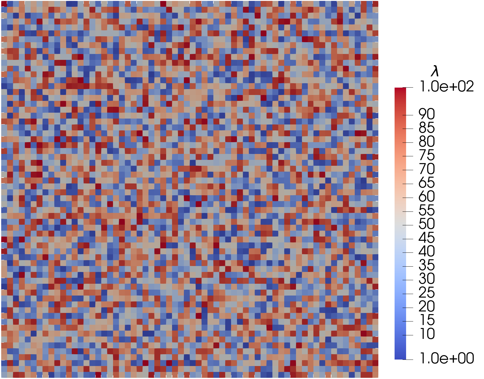

A fine-scale FEM reference solution is computed on a mesh with . We then compare this reference to approximate solutions obtained with both SLOD and a (coarse) FEM discretizations on meshes of increasing refinement . The right-hand side is chosen as the constant function . Figure 6.4 shows that SLOD exhibits a superexponential decay in the error, whereas the (coarse) FEM recovers its optimal rate of convergence once the mesh size approaches characteristic length .
A key aspect of the SLOD approximation arises from the upper bound in the error estimate (5.4), where the term can become dominant when is smoother. To illustrate this effect, we repeat the above test using the smooth right-hand side
| (6.1) |
which particularly belongs to .
Figure 6.5 shows how, in this scenario, the error is dominated by the approximation of the forcing term, which behaves as . Under the assumption that the localization error remains small, the second term in the right-hand side of (5.4) determines the overall convergence rate. Hence we observe for the -error and for the -error, consistent with a smooth forcing term in elasticity problems.
7. Conclusion
This paper introduced the Super-Localized Orthogonal Decomposition (SLOD) method for solving linear elasticity problems with highly heterogeneous (multiscale) microstructures. By constructing super-localized basis functions, SLOD improves upon the standard LOD method in both localization and computational efficiency, yet retains comparable theoretical guarantees on accuracy.
Extending the superlocalization framework to vector-valued elasticity underscores SLOD’s adaptability for diverse engineering and physical applications. Our numerical analysis demonstrates stability and convergence, instilling confidence in the method’s reliability. Meanwhile, the deal.II-based implementation showcases SLOD’s scalability and integration potential in modern high-performance computing workflows, an important step for addressing large-scale multiscale problems.
Several directions for future research remain open. First, while numerical evidence supports the super-exponential decay of the localization error, deeper theoretical proofs, particularly regarding the spectral geometry conjectures in the scalar setting, would further solidify SLOD’s foundations. Second, given the success of standard LOD for thermo- and poro-elasticity in [31, 16, 2], extending superlocalization to broader multiphysics problems where elasticity couples with other physical processes could yield significant new capabilities. Finally, enhancing our parallel implementation and incorporating adaptive refinements may expand SLOD’s applicability to even more demanding simulations.
References
- Africa et al. [2024] P. C. Africa, D. Arndt, W. Bangerth, B. Blais, M. Fehling, R. Gassmöller, T. Heister, L. Heltai, S. Kinnewig, M. Kronbichler, M. Maier, P. Munch, M. Schreter-Fleischhacker, J. P. Thiele, B. Turcksin, D. Wells, and V. Yushutin. The deal.ii library, version 9.6. Journal of Numerical Mathematics, 32(4):369–380, 2024. doi: 10.1515/jnma-2024-0137.
- Altmann et al. [2020] R. Altmann, E. Chung, R. Maier, D. Peterseim, and S.-M. Pun. Computational multiscale methods for linear heterogeneous poroelasticity. J. Comput. Math., 38(1):41–57, 2020.
- Altmann et al. [2021] R. Altmann, P. Henning, and D. Peterseim. Numerical homogenization beyond scale separation. Acta Numer., 30:1–86, 2021. doi: 10.1017/S0962492921000015.
- Babuška and Lipton [2011] I. Babuška and R. Lipton. Optimal local approximation spaces for generalized finite element methods with application to multiscale problems. Multiscale Model. Simul., 9(1):373–406, 2011. doi: 10.1137/100791051.
- Babuška et al. [2020] I. Babuška, R. Lipton, P. Sinz, and M. Stuebner. Multiscale-spectral GFEM and optimal oversampling. Comput. Methods Appl. Mech. Engrg., 364:112960, 2020. ISSN 0045-7825. doi: 10.1016/j.cma.2020.112960.
- Blanc and Le Bris [2023] X. Blanc and C. Le Bris. Homogenization Theory for Multiscale Problems: An introduction. MS&A. Springer Nature Switzerland, 2023. ISBN 9783031218323.
- Bonizzoni et al. [2024a] F. Bonizzoni, P. Freese, and D. Peterseim. Super-localized orthogonal decomposition for convection-dominated diffusion problems. BIT Numerical Mathematics, 64:33, 2024a. doi: 10.1007/s10543-024-01035-8.
- Bonizzoni et al. [2024b] F. Bonizzoni, M. Hauck, and D. Peterseim. A reduced basis super-localized orthogonal decomposition for reaction–convection–diffusion problems. J. Comput. Phys., 499:112698, 2024b. ISSN 0021-9991. doi: 10.1016/j.jcp.2023.112698.
- Brenner and Scott [2008] S. C. Brenner and L. R. Scott. The Mathematical Theory of Finite Element Methods. Springer, New York, third edition, 2008. ISBN 978-0-387-75933-3.
- Brenner et al. [2021] S. C. Brenner, J. C. Garay, and L.-Y. Sung. Additive Schwarz preconditioners for a localized orthogonal decomposition method. Electron. Trans. Numer. Anal., 54:234–255, 2021. doi: 10.1553/etna“˙vol54s234.
- Brenner et al. [2022] S. C. Brenner, J. C. Garay, and L-Y Sung. Multiscale finite element methods for an elliptic optimal control problem with rough coefficients. J. Sci. Comput. , 76, 2022. ISSN 1573-7691. doi: 10.1007/s10915-022-01834-7.
- Chung et al. [2023] E. Chung, Y. Efendiev, and T. Y Hou. Multiscale Model Reduction: Multiscale Finite Element Methods and Their Generalizations, volume 212. Springer Nature, 2023.
- Efendiev and Hou [2009] Y. Efendiev and T. Y. Hou. Multiscale Finite Element Methods: Theory and Applications. Surveys and Tutorials in the Applied Mathematical Sciences. Springer New York, NY, New York, 2009.
- Efendiev et al. [2013] Y. Efendiev, J. Galvis, and T. Y. Hou. Generalized multiscale finite element methods (GMsFEM). J. Comput. Phys., 251:116–135, 2013. ISSN 0021-9991. doi: 10.1016/j.jcp.2013.04.045.
- Freese et al. [2021] P. Freese, M. Hauck, and D. Peterseim. Super-localized orthogonal decomposition for high-frequency helmholtz problems. SIAM Journal on Scientific Computing, 46(4):A2377 – A2397, 2021. doi: 10.1137/21M1465950.
- Fu et al. [2019] S. Fu, R. Altmann, E. Chung, R. Maier, D. Peterseim, and S.-M. Pun. Computational multiscale methods for linear poroelasticity with high contrast. J. Comput. Phys., 395:286–297, 2019.
- Garay et al. [2024] J. C. Garay, H. Mohr, D. Peterseim, and C. Zimmer. Hierarchical super-localized orthogonal decomposition method, 2024. URL https://arxiv.org/abs/2407.18671.
- Hauck and Lozinski [2024] M. Hauck and A. Lozinski. A localized orthogonal decomposition method for heterogeneous stokes problems, 2024. URL https://arxiv.org/abs/2410.14514.
- Hauck and Målqvist [2022] M. Hauck and A. Målqvist. Super-localization of spatial network models. arXiv preprint 2210.07860, 2022. doi: 10.48550/ARXIV.2210.07860. URL https://arxiv.org/abs/2210.07860.
- Hauck and Peterseim [2022] M. Hauck and D. Peterseim. Super-localization of elliptic multiscale problems. Math. Comp., 92(342):981–1003, 2022. doi: 10.1090/mcom/3798.
- Hauck et al. [2024] M. Hauck, H. Mohr, and D. Peterseim. A simple collocation-type approach to numerical stochastic homogenization, 2024. arXiv e-print 2404.01732.
- Henning and Persson [2016] P. Henning and A. Persson. A multiscale method for linear elasticity reducing Poisson locking. Comput. Methods Appl. Mech. Engrg., 310:156–171, 2016. ISSN 0045-7825. doi: 10.1016/j.cma.2016.06.034. URL https://doi.org/10.1016/j.cma.2016.06.034.
- Henning and Peterseim [2013] P. Henning and D. Peterseim. Oversampling for the multiscale finite element method. Multiscale Model. Simul., 11(4):1149–1175, 2013. ISSN 1540-3459. doi: 10.1137/120900332.
- Hou and Wu [1997] T. Y. Hou and X.-H. Wu. A multiscale finite element method for elliptic problems in composite materials and porous media. J. Comput. Phys., 134(1):169–189, 1997. ISSN 0021-9991. doi: 10.1006/jcph.1997.5682.
- Klawonn et al. [2018] A. Klawonn, M. Kühn, and O. Rheinbach. Adaptive FETI-DP and BDDC methods with a generalized transformation of basis for heterogeneous problems. Electron. Trans. Numer. Anal., 49:1–27, 2018. doi: 10.1553/etna˙vol49s1.
- Kornhuber et al. [2018] R. Kornhuber, D. Peterseim, and H. Yserentant. An analysis of a class of variational multiscale methods based on subspace decomposition. Math. Comp., 87(314):2765–2774, 2018. ISSN 0025-5718. doi: 10.1090/mcom/3302.
- Ma [2024] C. Ma. A unified framework for multiscale spectral generalized fems and low-rank approximations to multiscale pdes, 2024. URL https://arxiv.org/abs/2311.08761.
- Ma et al. [2022] C. Ma, R. Scheichl, and T. Dodwell. Novel design and analysis of generalized finite element methods based on locally optimal spectral approximations. SIAM Journal on Numerical Analysis, 60(1):244–273, 2022. doi: 10.1137/21M1406179. URL https://doi.org/10.1137/21M1406179.
- Madureira and Sarkis [2021] A. L. Madureira and M. Sarkis. Hybrid localized spectral decomposition for multiscale problems. SIAM J. Numer. Anal., 59(2):829–863, 2021. doi: 10.1137/20M1314896.
- Maier [2021] R. Maier. A high-order approach to elliptic multiscale problems with general unstructured coefficients. SIAM J. Numer. Anal., 59(2):1067–1089, 2021. doi: 10.1137/20M1364321.
- Mlqvist and Persson [2017] A. Mlqvist and A. Persson. A generalized finite element method for linear thermoelasticity. ESAIM Math. Model. Numer. Anal., 51(4):1145–1171, 2017. ISSN 0764-583X. doi: 10.1051/m2an/2016054. URL https://doi.org/10.1051/m2an/2016054.
- Mlqvist and Peterseim [2014] A. Mlqvist and D. Peterseim. Localization of elliptic multiscale problems. Math. Comp., 83(290):2583–2603, 2014. ISSN 0025-5718. doi: 10.1090/S0025-5718-2014-02868-8.
- Mlqvist and Peterseim [2020] A. Mlqvist and D. Peterseim. Numerical Homogenization by Localized Orthogonal Decomposition. Society for Industrial and Applied Mathematics (SIAM), Philadelphia, 2020. ISBN 978-1-611976-44-1.
- Owhadi [2015] H. Owhadi. Bayesian numerical homogenization. Multiscale Model. Simul., 13(3):812–828, 2015. ISSN 1540-3459. doi: 10.1137/140974596.
- Owhadi [2017] H. Owhadi. Multigrid with rough coefficients and multiresolution operator decomposition from hierarchical information games. SIAM Rev., 59(1):99–149, 2017.
- Owhadi and Scovel [2019] H. Owhadi and C. Scovel. Operator-Adapted Wavelets, Fast Solvers, and Numerical Homogenization: From a Game Theoretic Approach to Numerical Approximation and Algorithm Design. Cambridge University Press, Cambridge, 2019. ISBN 978-1-108-48436-7.
- Owhadi et al. [2014] H. Owhadi, L. Zhang, and L. Berlyand. Polyharmonic homogenization, rough polyharmonic splines and sparse super-localization. ESAIM Math. Model. Numer. Anal. (M2AN), 48(2):517–552, 2014. ISSN 0764-583X. doi: 10.1051/m2an/2013118. URL http://dx.doi.org/10.1051/m2an/2013118.
- Peterseim and Scheichl [2016] D. Peterseim and R. Scheichl. Robust numerical upscaling of elliptic multiscale problems at high contrast. Comput. Methods Appl. Math., 16(4):579–603, 2016. ISSN 1609-4840. doi: 10.1515/cmam-2016-0022.
- Peterseim et al. [2024] D. Peterseim, J. Wärnegrd, and C. Zimmer. Super-localised wave function approximation of bose-einstein condensates. J. Comput. Phys., 510:113097, 2024. doi: 10.1016/j.jcp.2024.113097.
