Gravitational Effective Field Theories and Black Hole Mechanics

In short then, General Relativity is a mature, successful physical theory of gravity, standing on strong mathematical foundations. However, there are longstanding mysteries in gravitational physics which GR does not provide any insight into. The so-called "horizon problem" and "flatness problem" of cosmology can be resolved via a rapid period of acceleration in the early universe known as inflation, but exactly how this is driven in GR remains unanswered. "Dark matter" plays a crucial role in the formation of galaxies and the expansion of the universe, but its origin and description remain unknown. The value of the cosmological constant as measured by astronomical observations is much, much smaller (at least 60 order of magnitude Bousso:2008 ) than expected from calculations of the vacuum energy of the standard model.

To investigate these cosmological mysteries, many "modified" theories of gravity have been proposed that aim to produce the observed gravitational phenomena at cosmological scales. See Clifton:2011jh for a thorough review of the area. Most proposals make a modification of the Einstein-Hilbert action of GR to some more complicated action involving the metric and other gravitational fields and matter fields, $\psi_{I}$:

Most proposals stick to the core symmetry that underpins GR: diffeomorphism invariance. In these cases $\mathcal{L}(g_{\mu\nu},\psi_{I})$ must be a scalar under coordinate changes. Examples include $f(R)$ gravity Nojiri:2006ri , scalar-tensor theories such as Brans-Dicke theory Nariai:1969 and Horndeski theory Charmousis:2011bf , and higher dimensional theories such as Kaluza-Klein theory Freund:1982pg . Constraining these theories using astronomical and gravitational wave data is a highly active area of research, but we do not yet have a candidate that has emerged as an obvious improvement on GR. Additionally, many of these theories suffer from instabilities or so-called "ghost" degrees of freedom, and proofs of the well-posedness of their equations of motion are lacking, thus they often stand on shaky mathematical ground.

Perhaps more fundamentally than the phenomenological concerns of the above, GR predicts its own failure through the formation of singularities - points where curvatures and forces become infinite - and thus some deeper theory must take its place in these scenarios. GR is a classical field theory, and is not formulated in the mathematical language of operators that is needed to describe quantum mechanical effects that would presumably become important in the high energy regime near a singularity. One can hope that - like the other famous classical field theory, electromagnetism - GR can be formulated as a quantum field theory, however this presents many difficulties. For example, all other quantum field theories rely on a fixed background spacetime, whereas in GR the spacetime is the fundamental dynamical object. In quantum theories, states evolve through some fixed notion of time according to the Hamiltonian operator, whereas in GR the very notion of time is dependent on the state of the matter via the Einstein equations. Another major stumbling block is the fact that GR is "non-renormalizable" as a quantum field theory, meaning that it loses all predictive power at high energies.

With such manifest difficulties, we must change perspective. Rather than treating GR (or one of the modified theories above) as the fundamental theory of gravity to be quantized, we should instead view GR merely as the classical low-energy limit of some deeper underlying quantum gravity theory that is valid at arbitrarily high energies (so-called UV-complete). Proposals for such quantum gravity theories include string theory and loop quantum gravity. Experimentally probing any of these theories has proven extremely difficult, however there is hope for the future as our gravitational wave detectors improve and we are able to detect higher-energy gravitational events. In this case, we should study the corrections to GR these UV-complete theories will produce, and whether objects like black holes behave as expected. Developing the mathematical theory around these corrections will also help when trying to constrain these theories through observation. In this thesis, we shall use the framework of Effective Field Theory (EFT) to perform these studies.

A feature of the physics of the universe is that it can be split into distinct energy scales. We need not know the detailed mechanics of quark-to-quark interactions to describe the classical dynamics of billiard balls, which in turn are governed by different equations from the formation of galaxies. Qualitatively different structures emerge at varying energy scales, with each scale not interacting with the others. The underlying theory of physics describing the universe is assumed to be the same everywhere, so why can we neglect high energy physics when we are probing lower energy phenomena? This feature is called decoupling and can be described mathematically by Effective Field Theories.

Suppose we have some grand, UV-complete theory, $\mathcal{L}(\phi,\psi)$, which describes the physics of two fields $\phi$ and $\psi$. Suppose the fields have mass parameters $m_{\phi}$ and $m_{\psi}$, which roughly correspond to the lowest possible energy states of the fields. Generally, these scales will be very different, say $m_{\phi}\ll m_{\psi}$, in which case $\psi$ is some "heavy" high energy field, and $\phi$ is some "light" low energy field. If we can only probe the physics observationally at low energies, then by conservation of energy, we will only be able to study the behaviour of $\phi$, for example $\phi-\phi$ scattering amplitudes or its classical behaviour. The effect of $\psi$ on the physics of $\phi$ will still be there (because, for example, $\psi$ can be virtually created then destroyed in a scattering process), but we are unable to measure $\psi$ directly. This can be represented by "integrating out" the $\psi$ dependence in the theory’s path integral, resulting in an "effective" Lagrangian $\mathcal{L}_{\text{eff}}(\phi)$:

Why should we expect $\mathcal{L}_{\text{eff}}(\phi)$ to still be local? The answer is due to the uncertainty principle: virtual production of particles with energy $\Delta E\sim m_{\psi}$ can only result in the particles existing for $\Delta t\sim 1/m_{\psi}$, which is effectively instantaneous to our low energy probes. Similarly, the effects must be local in space by considering the momentum of $\psi$ particles. Therefore, $\mathcal{L}_{\text{eff}}(\phi)$ will be a sum of local operators made from $\phi$. These operators can be of any dimension, but since $1/m_{\psi}$ sets the scale of the locality, the coefficients of the operators will have appropriate factors of $1/m_{\psi}$ in order to make them the same dimension overall:

where $O_{D}(\phi)$ is some local operator of dimension $D$, $c_{D}$ are dimensionless constants, and $A$ is some overall dimensionful factor. If we know that $\phi$ obeys particular symmetries, then the operators present in (1.4) must also obey those symmetries. Physical observables such as scattering amplitudes of $\phi$ at energy $E$ will then be a power series in $E/m_{\psi}$, and we can truncate $\mathcal{L}_{\text{eff}}(\phi)$ to any order in $1/m_{\psi}$ to get predictions accurate up to that order in $E/m_{\psi}$.

The crucial fact about this procedure is that the form of (1.4) is completely agnostic about the details of the UV-complete theory $\mathcal{L}(\phi,\psi)$. Only the precise values of the coefficients $c_{D}$ depend on the details of $\mathcal{L}(\phi,\psi)$, but in theory we can measure the value of the $c_{D}$ up to some order by performing sufficiently accurate observations of the low energy behaviour of $\phi$. In particular, even though (1.4) may have infinitely many terms, to obtain predictions up to a particular order in $E/m_{\psi}$, we only need finitely many terms. Thus we can see how high energy physics naturally decouples from low energy physics, so long as we only probe at a particular scale.

Let us now discuss a specific example of this procedure. We will do this in a setting where we already have the UV-complete theory: the interactions between photons and electrons in flat space, which are determined by quantum electrodynamics (QED). In this theory, photons are described by a massless spin-one gauge field $A_{\mu}$, and electrons are described by a Dirac spinor field $\psi$. The QED Lagrangian is

where $F_{\mu\nu}=\partial_{\mu}A_{\nu}-\partial_{\nu}A_{\mu}$, and $-e$ and $m_{e}$ are respectively the charge and mass of the electron. The two particles in this theory have very different mass parameters: the photon is massless whereas $m_{e}$ is non-zero. Therefore, we can treat the photon as a light field and the electron as a heavy field. If we only want to study the physics of the photon at energies $E\ll m_{e}$ then we should be able to integrate out the electron from $\mathcal{L}(A_{\mu},\psi)$ to produce an effective action $\mathcal{L}_{eff}(A_{\mu})$. This effective action should predict exactly the same photon physics as the QED action, order-by-order in $E/m_{e}$.

What will $\mathcal{L}_{eff}(A_{\mu})$ look like? The QED action has various symmetries: Lorentz invariance, invariance under a gauge transformation $A_{\mu}\rightarrow A_{\mu}+\partial_{\mu}\chi$, charge conjugation invariance and parity invariance. The effective action will inherit these symmetries. Moreover, it will be a sum of terms of increasing operator dimension with associated factors of $1/m_{e}$. Therefore it will be of the form

where each $\mathcal{L}_{n}$ is a sum of terms with dimension $n$ that obey the above symmetries¹¹1Terms with odd dimension are forbidden by these symmetries.. The only possible dimension 4 term is $F_{\mu\nu}F^{\mu\nu}$, and we can always rescale $\mathcal{L}_{eff}$ to take

There is also only one possible term in $\mathcal{L}_{6}$ (up to total derivatives) which is of the form

where $a_{1}$ is a dimensionless constant. Terms such as $F^{\mu\nu}\partial^{\rho}\partial_{\rho}F_{\mu\nu}$ can be rewritten in terms of the above using the identity $\partial_{\rho}F_{\mu\nu}+\partial_{\mu}F_{\nu\rho}+\partial_{\nu}F_{\rho\mu}=0$ and integrating by parts. Similarly the set of terms in $\mathcal{L}_{8}$ can be expressed as

where $\tilde{F}_{\mu\nu}=\frac{1}{2}\epsilon_{\mu\nu\rho\sigma}F^{\rho\sigma}$ and $b_{1}$, $b_{2}$ are dimensionless constants. Note that terms with odd numbers of $F$’s are forbidden by charge-conjugation invariance, which sends $F_{\mu\nu}\rightarrow-F_{\mu\nu}$.

One can continue to write down higher and higher order terms in $\mathcal{L}_{eff}$. However, it turns out that we can simplify $\mathcal{L}_{6}$ and $\mathcal{L}_{8}$ further by making a field redefinition. If we define $A^{\prime}_{\mu}$ by

for some tensor $T_{\mu}$, then $\mathcal{L}_{4}$ can be rewritten as

Integrating by parts, the first order change in $\mathcal{L}_{4}$ is $\frac{1}{m_{e}^{2}}(\partial_{\mu}F^{\prime\mu\nu})T_{\nu}$. Therefore we can pick $T_{\mu}$ to eliminate any term proportional to $\partial_{\mu}F^{\prime\mu\nu}$ in the effective action, order-by-order in $1/m_{e}$. For example, choosing $T_{\mu}=-a_{1}\partial^{\rho}F^{\prime}_{\rho\nu}$ will eliminate the remaining term in $\mathcal{L}_{6}$. Similarly, all $\partial_{4}F^{2}$ terms in $\mathcal{L}_{8}$ can be eliminated in this way Burgess:2020 . Therefore, dropping the ’s, we can write our effective action as

with the ellipse denoting terms with dimension 10 or above.

Note that up until this point, we have not used the specifics of the QED Lagrangian apart from its symmetries. Any UV-complete theory of the photon and electron which shares those symmetries will produce an effective action of the form (1.12). It is only the specific values of the constants $b_{1},b_{2},...$ that will depend on the specifics of QED. In order to calculate what these constants are in the case of QED, there are two routes forward: i) actually perform the "integrating out" of the electron in the path integral, or ii) compare predictions of QED to that of the effective action. The first is exceedingly difficult; the second is only tediously difficult.

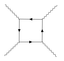
We can sketch how one would calculate $b_{1}$ and $b_{2}$ through the second route. This is done by comparing the predictions of the $2\rightarrow 2$ photon scattering amplitudes in the two theories, to leading order in $E/m_{e}$, where $E$ is the centre-of-mass energy of the photons. In QED, the leading order contributions to this scattering process come from box graphs of the form in Figure 1.1 while in the effective action they come from the vertex interactions represented by the two terms in $\mathcal{L}_{8}$ (see Figure 1.2). In both cases, one finds the amplitudes go as $(E/m_{e})^{4}$. Agreement of the two calculations implies Burgess:2020

where $\alpha$ is the fine-structure constant. With these values of the $b_{1}$, $b_{2}$, the effective action (1.12) truncated at the ellipse is known as the Euler-Heisenberg EFT; it describes the physics of the photon to order $(E/m_{e})^{4}$ in the regime $E\ll m_{e}$.

EFT techniques are used in many other areas of QED Caswell:1985ui , as well as QCD Hong:1998tn , Landau theory Polchinski:1992ed , condensed matter physics Shankar:1996 and in gravity, as we shall discuss next. A thorough review of the EFT procedure can be found in Burgess:2020 or Donoghue:1992dd .

In the above example, we constructed a low energy EFT from a known UV-complete theory. However, the general form of that EFT was independent of the specifics of the UV-complete theory. This is the great usefulness of EFTs: we can parameterize and quantify corrections to a known low-energy theory in the absence of any knowledge about its UV completion. Importantly for our purposes, this is exactly the framework we need for describing corrections to GR! We now discuss how this is achieved; see Burgess:2004 or Donoghue:2012zc for thorough reviews of gravitational EFTs.

We know that GR matches observation to excellent precision on energy scales such as those of planetary orbits in our solar system and the deflection of light around the sun. Therefore, the lowest order terms in any effective field theory of gravity (at least in regimes where other light matter fields can be neglected) must be those from the Einstein-Hilbert action

The metric has vanishing mass term, hence its mass parameter is $m_{g}=0$. It is indeed a "light" field. What should we take as the "heavy" mass scale $m$ (our equivalent of $m_{\psi}$ from above)? This can be whatever is the smallest scale we have integrated out, for example the electron mass if we are studying applications at energies less than the mass of all elementary particles. Regardless, for convenience we shall define $l=1/m$ and call $l$ our "UV-scale".

$R$ has mass dimension 2 as it involves two derivatives of the metric, which is itself dimensionless. The EFT corrections in the ellipsis can include all higher mass dimension quantities made from $g_{\mu\nu}$, i.e., terms with more derivatives. However, we know that GR has a symmetry which we expect to hold in the UV-complete theory: diffeomorphism invariance. Thus we restrict ourselves to including any possible scalar made from contractions or covariant derivatives of the Riemann tensor²²2In a $d$-dimensional spacetime, we should also include the volume form $\epsilon_{\mu_{1}...\mu_{d}}$. In even dimensions, only terms with even numbers of derivatives can appear in a pure gravity EFT, but in odd dimensions we can use $\epsilon_{\mu_{1}...\mu_{d}}$ to construct terms with an odd number of derivatives.:

Note that total derivative terms such as $\nabla_{\mu}\nabla^{\mu}R$ are redundant and can be ignored so long as we are only concerned with observables like the classical equations of motion or perturbative scattering amplitudes that do not depend on the topology of the spacetime. Furthermore, the higher derivative terms are not unique under a field redefinition of the metric, a fact which we can use to eliminate more coefficients in a similar fashion to the low-energy photon EFT example of the previous section. A field redefinition of the form $g_{\mu\nu}\rightarrow g_{\mu\nu}+l^{2}(a\Lambda g_{\mu\nu}+bRg_{\mu\nu}+cR_{\mu\nu})$ with appropriate constants $a,b,c$ can be used to push anything proportional to $R_{\mu\nu}$ up to arbitrarily high order in $l$ Burgess:2004 . This can be used to bring the 4-derivative terms into the form of a single term given by the Einstein-Gauss-Bonnet (EGB) Lagrangian ³³3This process may also renormalize the values of $\Lambda$ and $G$.:

where the generalized Kronecker delta is

For general spacetime dimension $d>4$, this is as far as we can go, in which case EGB gravity is the leading order EFT correction to GR. However, in $d=4$ dimensions the 4-derivative EGB term is topological and can be neglected⁴⁴4In fact, for $d=4$ there is another topological term of the form $R_{\mu\nu\rho\sigma}R_{\alpha\beta}{}^{\rho\sigma}\epsilon^{\mu\nu\alpha\beta}$ which we ignore for the same reasons.. Therefore we can eliminate all order $l^{2}$ contributions to $\mathcal{L}_{eff}$. We can perform a similar procedure Endlich:2017 ; Cano:2019 to reduce the set of 6-derivative terms to the following:

Note the above reduction only holds if we are in vacuum, i.e., in a regime where other light matter fields can be neglected. We could instead look at situations where such matter fields are important. For example around a highly charged black hole, we should include the electromagnetic field $F_{\mu\nu}$. In this case, $\mathcal{L}_{\text{eff}}(g_{\mu\nu},F_{\rho\sigma})$ will be the Einstein-Maxwell Lagrangian supplemented by all higher mass dimension contractions and covariant derivatives of $R_{\mu\nu\rho\sigma}$ and $F_{\mu\nu}$.

Finally, we note that we have included the cosmological constant $\Lambda$ here without any factors of $l$. Naively in EFT, we should expect 0-derivative terms to come with a factor $1/l^{2}$ relative to the 2-derivative $R$. However, for somewhat mysterious reasons (see the cosmological constant problem), observations find that $\Lambda$ is extremely small and so we will assume it instead scales as $l^{0}$.

Above, we heuristically formulated effective field theory in terms of quantum field theory. However there may be a regime where both the classical approximation is valid and the effective field theory corrections make an observable effect. Such a regime is often assumed when making practical applications to gravity, for example in cosmology and in numerical simulations of black hole mergers in modified theories of gravity East:2020hgw . We shall assume the existence of this regime in this thesis.

From a classical perspective, "integrating out" $\psi$ from our UV-complete theory $\mathcal{L}(\phi,\psi)$ is equivalent to eliminating $\psi$ by formally solving the classical equation of motion for $\psi$ order-by-order in $l$ in terms of $\phi$. Under what conditions is this expansion in $l$ valid? Furthermore, the EFT equation of motion for $\phi$ arising from $\mathcal{L}_{\text{eff}}$ will generally involve higher than second order derivatives - can we avoid needing additional initial data and can a well-posed initial value problem be formulated? In general, the EFT equations will result in "runaway" solutions that blow up in time - can we identify and eliminate such unphysical solutions? Moreover, are the classical solutions of the EFT theory even close to some classical solution of the underlying UV theory? Broadly, these are unanswered questions in the full generality of gravitational EFTs, although there has been much discussion in the area Flanagan:1996gw Burgess:2014lwa Solomon:2017nlh Allwright:2018rut Cayuso:2023xbc Reall:2021ebq .

There is, however, a well-motivated proposal for the "regime of validity" of a classical EFT in which these questions are all expected to be answered in the affirmative. We saw that we should expect our effective Lagrangian $\mathcal{L}_{\text{eff}}(\phi)$ to be local if and only if we probe the light field $\phi$ at energy scales much less than the mass scale we have integrated out. From a classical perspective, this corresponds to a classical solution $\phi(x^{\mu})$ varying on length/time scales that are much longer than the UV-scale $l$. We can formulate this mathematically as follows. Assume that we have a 1-parameter family of solutions $\phi(x^{\mu},L)$ to the EFT equations of motion on some region of spacetime $\mathcal{R}$, such that any $n$-derivative quantity made from $\phi$ is uniformly bounded above by $c_{n}/L^{n}$, i.e.,

for some dimensionless ($L$-independent) constant $c_{n}$. $L$ can represent the smallest length/time scale associated to the solution, e.g. some timescale in the dynamics or some typical length scale. Then $\phi(x^{\mu},L)$ is said to lie in the regime of validity of the EFT if $L\gg l$.

Any solution that lies outside this regime must have some scale that is comparable to the UV-scale. In that scenario however, we should not expect our effective action to be valid because the energies of the heavy and light fields cannot be separated! Thus such solutions should be immediately disregarded because they are solutions to a theory of physics inapplicable to their situation. If we are in a scenario where we trust our EFT, then solutions that lie in the regime of validity are the only sensible ones to consider.

Note that when the light fields are gauge fields, we must add to the above definition that it holds in some choice of gauge. For example in the case of the metric, we say it lies in the regime of validity if there is some particular choice of coordinates in which the above conditions hold. It does not need to hold in all coordinate systems - indeed one can always make a diffeomorphism that will take the solution out of the regime of validity, for example by adding highly oscillatory behaviour or a coordinate singularity. In this sense the definition is not covariant, but this seems unavoidable in any notion of regime of validity of EFT due to its very purpose being to describe a separation of scales.

Mathematically, this definition of regime of validity is useful because it provides us with a dimensionless small parameter, $l/L$, which we can use to bound the size of terms in the EFT equations of motion or solution. For example, the EFT equation of motion for the metric in the general vacuum gravity EFT (1.15) is of the form

where $E_{\mu\nu}^{(n)}$ comes from the $(n+2)$-derivative part of $\mathcal{L}_{\text{eff}}(g_{\mu\nu})$ and hence is a sum of $(n+2)$-derivative terms itself. Therefore, if $g_{\mu\nu}$ lies in the regime of validity of the EFT in some coordinate system then in that coordinate system $l^{n}E_{\mu\nu}^{(n)}=O(l^{n}/L^{n+2})$ and so the higher derivative terms are less and less important. Furthermore, in practice we will only ever know finitely many of the coefficients in $\mathcal{L}_{\text{eff}}$, so there will be some maximal $N$ for which we know all the terms with $N+1$ or fewer derivatives. In this case we only fully know the $\Lambda g_{\mu\nu}+R_{\mu\nu}-\frac{1}{2}Rg_{\mu\nu}+\sum_{n=1}^{N-1}l^{n}E_{\mu\nu}^{(n)}$ part of the equations of motion, but in the regime of validity we can still state

We can then make progress on proving properties of these equations, even though we do not know the precise value of the right hand side. In general, we will suppress the explicit $L$-dependence and just write the RHS as $O(l^{N})$. The factors of $L$ can be reinstated by dimensional analysis.

For a particular toy EFT model of a scalar field in a "Mexican hat" potential, Reall:2021ebq has rigorously demonstrated that in the regime of validity all of the above questions regarding the mathematical soundness of the EFT equations can be resolved. The definition has also been used in applications such as black hole entropy Hollands:2022 Deo:2023 and in proving well-posedness Figueras:2024bba of gravitational EFTs. In this thesis, we shall not consider general solutions to gravitational EFT equations of motion, but only ones that lie within the regime of validity of the EFT.

Suppose we would like to study the evolution of a collection of classical fields $u_{I}$, with $I=1,\ldots,N$. For simplicity, let us suppose there are no gauges involved and that we have a fixed notion of time and space, $x^{\mu}=(x^{0},x^{i})$. After an initial instant of time, $x^{0}=0$, suppose the evolution of $u_{I}$ is governed by a set of equations of motion involving $u_{I}$ and its derivatives. In this Chapter, we shall be concerned with second order equations of motion, i.e. those of the form

References

• (1) Y. Fourès-Bruhat, “Théorème d’existence pour certains systèmes d’équations aux dérivées partielles non linéaires,” Acta Math. 88, 141 - 225, (1952) doi:10.1007/BF02392131
• (2) T. W. Baumgarte and S. L. Shapiro, “On the numerical integration of Einstein’s field equations,” Phys. Rev. D 59, 024007 (1998) doi:10.1103/PhysRevD.59.024007 [arXiv:gr-qc/9810065 [gr-qc]].
• (3) M. Shibata and T. Nakamura, “Evolution of three-dimensional gravitational waves: Harmonic slicing case,” Phys. Rev. D 52, 5428-5444 (1995) doi:10.1103/PhysRevD.52.5428
• (4) O. Sarbach, G. Calabrese, J. Pullin and M. Tiglio, “Hyperbolicity of the BSSN system of Einstein evolution equations,” Phys. Rev. D 66, 064002 (2002) doi:10.1103/PhysRevD.66.064002 [arXiv:gr-qc/0205064 [gr-qc]].
• (5) G. Nagy, O. E. Ortiz and O. A. Reula, “Strongly hyperbolic second order Einstein’s evolution equations,” Phys. Rev. D 70, 044012 (2004) doi:10.1103/PhysRevD.70.044012 [arXiv:gr-qc/0402123 [gr-qc]].
• (6) R. Schoen and S.T. Yau, “Proof of the positive mass theorem. II,” Comm.Math. Phys. 79, 231–260 (1981) https://doi.org/10.1007/BF01942062
• (7) E. Witten, “A new proof of the positive energy theorem,” Comm. Math. Phys. 80, 381 (1981) https://doi.org/10.1007/BF01208277
• (8) J. M. Bardeen, B. Carter and S. W. Hawking, “The Four laws of black hole mechanics,” Comm. Math. Phys. 31, 161–170 (1973) https://doi.org/10.1007/BF01645742
• (9) S.W. Hawking, “Particle creation by black holes,” Comm. Math. Phys. 43, 199–220 (1975) https://doi.org/10.1007/BF02345020
• (10) R. Bousso, “The cosmological constant,” Gen Relativ Gravit 40, 607–637 (2008). https://doi.org/10.1007/s10714-007-0557-5
• (11) T. Clifton, P. G. Ferreira, A. Padilla and C. Skordis, “Modified Gravity and Cosmology,” Phys. Rept. 513 (2012), 1-189 doi:10.1016/j.physrep.2012.01.001 [arXiv:1106.2476 [astro-ph.CO]].
• (12) S. Nojiri and S. D. Odintsov, “Introduction to modified gravity and gravitational alternative for dark energy,” eConf C0602061 (2006), 06 doi:10.1142/S0219887807001928 [arXiv:hep-th/0601213 [hep-th]].
• (13) H. Nariai, “Gravitational Instability in the Brans-Dicke Cosmology,” Progress of Theoretical Physics, 42, 3, (1969), 544–554, https://doi.org/10.1143/PTP.42.544
• (14) C. Charmousis, E. J. Copeland, A. Padilla and P. M. Saffin, “General second order scalar-tensor theory, self tuning, and the Fab Four,” Phys. Rev. Lett. 108 (2012), 051101 doi:10.1103/PhysRevLett.108.051101 [arXiv:1106.2000 [hep-th]].
• (15) P. G. O. Freund, “Kaluza-Klein Cosmologies,” Nucl. Phys. B 209 (1982), 146 doi:10.1016/0550-3213(82)90106-7
• (16) C. P. Burgess, “Introduction to Effective Field Theory", Cambridge University Press, (2020) doi:10.1017/9781139048040
• (17) J. F. Donoghue, E. Golowich and B. R. Holstein, “Dynamics of the standard model,” Camb. Monogr. Part. Phys. Nucl. Phys. Cosmol. 2 (1992), 1-540 CUP, 2014, doi:10.1017/CBO9780511524370
• (18) W. E. Caswell and G. P. Lepage, “Effective Lagrangians for Bound State Problems in QED, QCD, and Other Field Theories,” Phys. Lett. B 167 (1986), 437-442 doi:10.1016/0370-2693(86)91297-9
• (19) D. K. Hong, “An Effective field theory of QCD at high density,” Phys. Lett. B 473 (2000), 118-125 doi:10.1016/S0370-2693(99)01472-0 [arXiv:hep-ph/9812510 [hep-ph]].
• (20) J. Polchinski, “Effective field theory and the Fermi surface,” (1992) [arXiv:hep-th/9210046 [hep-th]].
• (21) R. Shankar, “Effective Field Theory in Condensed Matter Physics,” lecture given at Boston Colloquium for the Philosophy of Science, Boston, Mass., 1996, [arXiv:cond-mat/9703210]
• (22) C. P. Burgess, “Quantum Gravity in Everyday Life: General Relativity as an Effective Field Theory", Living Rev. Relativ. 7, no.5 (2004) doi:10.12942/lrr-2004-5
• (23) J. F. Donoghue, “The effective field theory treatment of quantum gravity,” AIP Conf. Proc. 1483 (2012) no.1, 73-94 doi:10.1063/1.4756964 [arXiv:1209.3511 [gr-qc]].
• (24) S. Endlich, V. Gorbenko, J. Huang, and L. Senatore, “An effective formalism for testing extensions to General Relativity with gravitational waves,” JHEP 09 (2017) 122, [arXiv:1704.01590].
• (25) P.A. Cano and A. Ruipérez, “Leading higher-derivative corrections to Kerr geometry,” J. High Energ. Phys. 2019, 189 (2019). https://doi.org/10.1007/JHEP05(2019)189
• (26) W. E. East and J. L. Ripley, “Evolution of Einstein-scalar-Gauss-Bonnet gravity using a modified harmonic formulation,” Phys. Rev. D 103 (2021) no.4, 044040 doi:10.1103/PhysRevD.103.044040 [arXiv:2011.03547 [gr-qc]].
• (27) E. E. Flanagan and R. M. Wald, “Does back reaction enforce the averaged null energy condition in semiclassical gravity?,” Phys. Rev. D 54, 6233-6283 (1996) doi:10.1103/PhysRevD.54.6233 [arXiv:gr-qc/9602052 [gr-qc]].
• (28) C. P. Burgess and M. Williams, “Who You Gonna Call? Runaway Ghosts, Higher Derivatives and Time-Dependence in EFTs,” JHEP 08 (2014), 074 doi:10.1007/JHEP08(2014)074 [arXiv:1404.2236 [gr-qc]].
• (29) A. R. Solomon and M. Trodden, “Higher-derivative operators and effective field theory for general scalar-tensor theories,” JCAP 02 (2018), 031 doi:10.1088/1475-7516/2018/02/031 [arXiv:1709.09695 [hep-th]].
• (30) G. Allwright and L. Lehner, “Towards the nonlinear regime in extensions to GR: assessing possible options,” Class. Quant. Grav. 36 (2019) no.8, 084001 doi:10.1088/1361-6382/ab0ee1 [arXiv:1808.07897 [gr-qc]].
• (31) R. Cayuso, P. Figueras, T. França and L. Lehner, “Self-Consistent Modeling of Gravitational Theories beyond General Relativity,” Phys. Rev. Lett. 131 (2023) no.11, 111403 doi:10.1103/PhysRevLett.131.111403
• (32) H. S. Reall and C. M. Warnick, “Effective field theory and classical equations of motion,” J. Math. Phys. 63 (2022) no.4, 042901 doi:10.1063/5.0075455 [arXiv:2105.12028 [hep-th]].
• (33) S. Hollands, Á. D. Kovács and H. S. Reall, “The second law of black hole mechanics in effective field theory,” JHEP 08 (2022), 258 doi:10.1007/JHEP08(2022)258 [arXiv:2205.15341 [hep-th]].
• (34) I. Deo, P. Dhivakar and N. Kundu, “Entropy-current for dynamical black holes in Chern-Simons theories of gravity,” JHEP 11 (2023), 114 doi:10.1007/JHEP11(2023)114 [arXiv:2306.12491 [hep-th]].
• (35) P. Figueras, A. Held and Á. D. Kovács, “Well-posed initial value formulation of general effective field theories of gravity,” [arXiv:2407.08775 [gr-qc]].
• (36) Á. D. Kovács and H. S. Reall, “Well-Posed Formulation of Scalar-Tensor Effective Field Theory,” Phys. Rev. Lett. 124, no.22, 221101 (2020) doi:10.1103/PhysRevLett.124.221101 [arXiv:2003.04327 [gr-qc]].
• (37) Á. D. Kovács and H. S. Reall, “Well-posed formulation of Lovelock and Horndeski theories,” Phys. Rev. D 101, no.12, 124003 (2020) doi:10.1103/PhysRevD.101.124003 [arXiv:2003.08398 [gr-qc]].
• (38) I. Davies and H. S. Reall, “Well-posed formulation of Einstein-Maxwell effective field theory,” Phys. Rev. D 106, 104019 (2022)
• (39) D. R. Noakes, “The Initial Value Formulation of Higher Derivative Gravity,” J. Math. Phys. 24, 1846-1850 (1983) doi:10.1063/1.525906
• (40) S. Deser and P. van Nieuwenhuizen, “One Loop Divergences of Quantized Einstein-Maxwell Fields,” Phys. Rev. D 10, 401 (1974) doi:10.1103/PhysRevD.10.401
• (41) C. R. T. Jones and B. McPeak, “The Black Hole Weak Gravity Conjecture with Multiple Charges,” JHEP 06, 140 (2020) doi:10.1007/JHEP06(2020)140 [arXiv:1908.10452 [hep-th]].
• (42) I. T. Drummond and S. J. Hathrell, “QED Vacuum Polarization in a Background Gravitational Field and Its Effect on the Velocity of Photons,” Phys. Rev. D 22, 343 (1980) doi:10.1103/PhysRevD.22.343
• (43) G. Horndeski, “Conservation of charge and the Einstein–Maxwell field equations J. Math. Phys. 17 (1980) doi:10.1063/1.522837
• (44) F. Abalos, F. Carrasco, É. Goulart and O. Reula, “Nonlinear electrodynamics as a symmetric hyperbolic system,” Phys. Rev. D 92, no.8, 084024 (2015) doi:10.1103/PhysRevD.92.084024 [arXiv:1507.02262 [gr-qc]].
• (45) L. E. Kidder, M. A. Scheel and S. A. Teukolsky, “Extending the lifetime of 3-D black hole computations with a new hyperbolic system of evolution equations,” Phys. Rev. D 64, 064017 (2001) doi:10.1103/PhysRevD.64.064017 [arXiv:gr-qc/0105031 [gr-qc]].
• (46) G. Papallo and H. S. Reall, “On the local well-posedness of Lovelock and Horndeski theories,” Phys. Rev. D 96, no.4, 044019 (2017) doi:10.1103/PhysRevD.96.044019 [arXiv:1705.04370 [gr-qc]].
• (47) G. Papallo, “On the hyperbolicity of the most general Horndeski theory,” Phys. Rev. D 96, no.12, 124036 (2017) doi:10.1103/PhysRevD.96.124036 [arXiv:1710.10155 [gr-qc]].
• (48) Á. D. Kovács, “Well-posedness of cubic Horndeski theories,” Phys. Rev. D 100, no.2, 024005 (2019) doi:10.1103/PhysRevD.100.024005 [arXiv:1904.00963 [gr-qc]].
• (49) R. M. Wald, “General Relativity,” Chicago Univ. Pr., 1984, doi:10.7208/chicago/9780226870373.001.0001
• (50) M. E. Taylor, “Pseudodifferential Operators and Nonlinear PDE,” (Birkhäuser, Boston, MA, 1991).
• (51) M. Alcubierre, J. C. Degollado and M. Salgado, “The Einstein-Maxwell system in 3+1 form and initial data for multiple charged black holes,” Phys. Rev. D 80 (2009), 104022 doi:10.1103/PhysRevD.80.104022 [arXiv:0907.1151 [gr-qc]].
• (52) H. S. Reall, “Causality in gravitational theories with second order equations of motion,” Phys. Rev. D 103, no.8, 084027 (2021) doi:10.1103/PhysRevD.103.084027 [arXiv:2101.11623 [gr-qc]].
• (53) S. W. Hawking and G. F. R. Ellis, “The large scale structure of space-time,” Vol. 1. Cambridge University Press, (1973).
• (54) R. Emparan and H. S. Reall, “A Rotating Black Ring Solution in Five Dimensions,” Phys. Rev. Lett. 88, 101101 (2002) doi:10.1103/PhysRevLett.88.101101
• (55) R. Penrose, “Gravitational collapse and space-time singularities,” Phys. Rev. Lett. 14 (1965) 57–59. doi:10.1103/PhysRevLett.14.57.
• (56) R. Penrose, “Gravitational collapse: The role of general relativity,” Riv. Nuovo Cim. 1 (1969) 252–276. doi:10.1023/A:1016578408204.
• (57) K. Akiyama, et al., “First M87 Event Horizon Telescope Results. I. The Shadow of the Supermassive Black Hole,” Astrophys. J. Lett. 875 (2019) L1. doi:10.3847/ 2041-8213/ab0ec7.
• (58) A. M. Ghez, B. L. Klein, M. Morris, E. E. Becklin, “High proper-motion stars in the vicinity of sagittarius a∗a*: Evidence for a supermassive black hole at the center of our galaxy,” The Astrophysical Journal 509 (2) (1998) 678–686. doi:10.1086/306528.
• (59) S. Gillessen, F. Eisenhauer, S. Trippe, T. Alexander, R. Genzel, F. Martins, T. Ott, “Monitoring stellar orbits around the Massive Black Hole in the Galactic Center,” Astrophys. J. 692 (2009) 1075–1109. doi:10.1088/0004-637X/692/2/1075.
• (60) P. T. Chrusciel, J. L. Costa, “On uniqueness of stationary vacuum black holes,” Géométrie différentielle, physique mathématique, mathématiques et société (I) : Volume en l’honneur de Jean Pierre Bourguignon, Astérisque, no. 321 (2008), pp. 195-265
• (61) S. W. Hawking, “Black holes in general relativity,” Commun. Math. Phys. 25 (1972) 152–166.
• (62) S. Hollands, A. Ishibashi and R. M. Wald, “A Higher dimensional stationary rotating black hole must be axisymmetric,” Commun. Math. Phys. 271 (2007), 699-722 doi:10.1007/s00220-007-0216-4 [arXiv:gr-qc/0605106 [gr-qc]].
• (63) V. Moncrief and J. Isenberg, “Symmetries of Higher Dimensional Black Holes,” Class. Quant. Grav. 25 (2008), 195015 doi:10.1088/0264-9381/25/19/195015 [arXiv:0805.1451 [gr-qc]].
• (64) H. Friedrich, I. Rácz, and R. M. Wald, “On the rigidity theorem for spacetimes with a stationary event horizon or a compact Cauchy horizon,” Commun. Math. Phys. 204 (1998) 691-707.
• (65) I. Rácz, “On further generalization of the rigidity theorem for spacetimes with a stationary event horizon or a compact Cauchy horizon,” Class. Quant. Grav. 17, 153 (2000)
• (66) A. D. Ionescu and S. Klainerman, “On the uniqueness of smooth, stationary black holes in vacuum,” Invent. Math. 175 (2008), 35 doi:10.1007/s00222-008-0146-6 [arXiv:0711.0040 [gr-qc]].
• (67) S. Hollands, A. Ishibashi and H. S. Reall, “A Stationary Black Hole Must be Axisymmetric in Effective Field Theory,” Commun. Math. Phys. 401 (2023) no.3, 2757-2791 doi:10.1007/s00220-023-04700-1 [arXiv:2212.06554 [gr-qc]].
• (68) C. Kehle and R. Unger, “Gravitational collapse to extremal black holes and the third law of black hole thermodynamics,” [arXiv:2211.15742 [gr-qc]].
• (69) B. S. Kay and R. M. Wald, “Theorems on the Uniqueness and Thermal Properties of Stationary, Nonsingular, Quasifree States on Space-Times with a Bifurcate Killing Horizon,” Phys. Rept. 207 (1991), 49-136 doi:10.1016/0370-1573(91)90015-E
• (70) J. D. Bekenstein, “Generalized second law of thermodynamics in black hole physics,” Phys. Rev. D 9 (1974), 3292-3300 doi:10.1103/PhysRevD.9.3292
• (71) V. Moncrief and J. Isenberg, “Symmetries of cosmological Cauchy horizons,” Commun. Math. Phys. 89 (1983) no.3, 387-413 doi:10.1007/BF01214662
• (72) A. C. Wall, “A Second Law for Higher Curvature Gravity,” Int. J. Mod. Phys. D 24 (2015) no.12, 1544014 doi:10.1142/S0218271815440149 [arXiv:1504.08040 [gr-qc]].
• (73) S. Bhattacharyya, P. Dhivakar, A. Dinda, N. Kundu, M. Patra and S. Roy, “An entropy current and the second law in higher derivative theories of gravity,” JHEP 09, 169 (2021) doi:10.1007/JHEP09(2021)169 [arXiv:2105.06455 [hep-th]].
• (74) S. Sarkar, “Black hole thermodynamics: general relativity and beyond,” Gen. Rel. Grav. 51 (2019) 63 [arXiv:1905.04466]
• (75) R. Ghosh and S. Sarkar, “Black Hole Zeroth Law in Higher Curvature Gravity,” Phys. Rev. D 102, no.10, 101503(R) (2020) doi:10.1103/PhysRevD.102.101503 [arXiv:2009.01543 [gr-qc]].
• (76) Bhattacharyya, S., Biswas, P., Dinda, A. et al. “The zeroth law of black hole thermodynamics in arbitrary higher derivative theories of gravity,” J. High Energ. Phys. 2022, 13 (2022). https://doi.org/10.1007/JHEP10(2022)013 [arXiv:2205.01648 [hep-th]].
• (77) I. Racz and R. M. Wald, “Global extensions of space-times describing asymptotic final states of black holes,” Class. Quant. Grav. 13 (1996), 539-553 doi:10.1088/0264-9381/13/3/017 [arXiv:gr-qc/9507055 [gr-qc]].
• (78) D. Sudarsky and R. M. Wald, “Extrema of mass, stationarity, and staticity, and solutions to the Einstein Yang-Mills equations,” Phys. Rev. D 46 (1992), 1453-1474 doi:10.1103/PhysRevD.46.1453
• (79) S. W. Hawking and J. B. Hartle, “Energy and angular momentum flow into a black hole,” Commun. Math. Phys. 27 (1972), 283-290 doi:10.1007/BF01645515
• (80) S. Gao and R. M. Wald, “The ‘Physical process’ version of the first law and the generalized second law for charged and rotating black holes,” Phys. Rev. D64 (2001) 084020, [gr-qc/0106071].
• (81) R. M. Wald, “Black hole entropy is the Noether charge,” Phys. Rev. D 48 (1993) no.8, R3427-R3431 doi:10.1103/PhysRevD.48.R3427 [arXiv:gr-qc/9307038 [gr-qc]].
• (82) T. Jacobson, G. Kang and R. C. Myers, “On black hole entropy,” Phys. Rev. D 49 (1994), 6587-6598 doi:10.1103/PhysRevD.49.6587 [arXiv:gr-qc/9312023 [gr-qc]].
• (83) V. Iyer and R. M. Wald, “Some properties of Noether charge and a proposal for dynamical black hole entropy,” Phys. Rev. D 50 (1994), 846-864 doi:10.1103/PhysRevD.50.846 [arXiv:gr-qc/9403028 [gr-qc]].
• (84) A. Mishra, S. Chakraborty, A. Ghosh and S. Sarkar, “On the physical process first law for dynamical black holes,” JHEP 09 (2018), 034 doi:10.1007/JHEP09(2018)034 [arXiv:1709.08925 [gr-qc]].
• (85) P. T. Chrusciel, E. Delay, G. J. Galloway and R. Howard, “The Area theorem,” Annales Henri Poincare 2 (2001), 109-178 doi:10.1007/PL00001029 [arXiv:gr-qc/0001003 [gr-qc]].
• (86) T. Jacobson, G. Kang and R. C. Myers, “Increase of black hole entropy in higher curvature gravity,” Phys. Rev. D 52 (1995), 3518-3528 doi:10.1103/PhysRevD.52.3518 [arXiv:gr-qc/9503020 [gr-qc]].
• (87) A. Chatterjee and S. Sarkar, “Physical process first law and increase of horizon entropy for black holes in Einstein-Gauss-Bonnet gravity,” Phys. Rev. Lett. 108, 091301 (2012) doi:10.1103/PhysRevLett.108.091301 [arXiv:1111.3021 [gr-qc]].
• (88) S. Sarkar and A. C. Wall, “Generalized second law at linear order for actions that are functions of Lovelock densities,” Phys. Rev. D 88 (2013), 044017 doi:10.1103/PhysRevD.88.044017 [arXiv:1306.1623 [gr-qc]].
• (89) S. Bhattacharjee, S. Sarkar and A. C. Wall, “Holographic entropy increases in quadratic curvature gravity,” Phys. Rev. D 92, 064006 (2015) doi:10.1103/PhysRevD.92.064006 [arXiv:1504.04706 [gr-qc]].
• (90) S. Bhattacharyya, P. Jethwani, M. Patra and S. Roy, “Reparametrization Symmetry of Local Entropy Production on a Dynamical Horizon,” [arXiv:2204.08447 [hep-th]].
• (91) P. Biswas, P. Dhivakar and N. Kundu “Non-minimal coupling of scalar and gauge fields with gravity: an entropy current and linearized second law,” JHEP 2022 36 (2022). https://doi.org/10.1007/JHEP12(2022)036 [arXiv:2206.04538v2 [hep-th]].
• (92) S. Hollands, R. M. Wald and V. G. Zhang, “Entropy of dynamical black holes,” Phys. Rev. D 110 (2024) no.2, 024070 doi:10.1103/PhysRevD.110.024070 [arXiv:2402.00818 [hep-th]].
• (93) I. Davies, “Zeroth and second laws of black hole mechanics in Einstein-Maxwell-scalar effective field theory,” Phys. Rev. D 109 (2024) no.8, 084051 doi:10.1103/PhysRevD.109.084051 [arXiv:2401.13075 [gr-qc]].
• (94) A. C. Wall and Z. Yan, “Linearised Second Law for Higher Curvature Gravity and Non-Minimally Coupled Vector Fields,” [arXiv:2402.05411 [gr-qc]].
• (95) I. Racz and R. M. Wald, “Extension of space-times with Killing horizon,” Class. Quant. Grav. 9, 2643-2656 (1992) doi:10.1088/0264-9381/9/12/008
• (96) S.  Weinberg, “Effective Field Theory for Inflation,” Phys. Rev. D 77 (2008) 123541, [arXiv:0804.4291 [hep-th]].
• (97) J. L. Friedman, K. Schleich and D. M. Witt, “Topological censorship,” Phys. Rev. Lett. 71 (1993), 1486-1489 [erratum: Phys. Rev. Lett. 75 (1995), 1872] doi:10.1103/PhysRevLett.71.1486 [arXiv:gr-qc/9305017 [gr-qc]].
• (98) T. Aubin, “Nonlinear analysis on manifolds, Monge-Ampère equations,” (Springer New York, 1982).
• (99) H. Lawson and M. Michelsohn, “Spin Geometry,” (PMS-38), Volume 38 (Princeton: Princeton University Press, 1990).
• (100) E. Hebey, “Nonlinear analysis on manifolds: Sobolev spaces and inequalities,” (American Mathematical Society, 2000).
• (101) An, YP., Li, L. “Static de-Sitter black holes abhor charged scalar hair,” Eur. Phys. J. C 83, 569 (2023), https://doi.org/10.1140/epjc/s10052-023-11758-7
• (102) P. Kanti, N. E. Mavromatos, J. Rizos, K. Tamvakis and E. Winstanley, “Dilatonic black holes in higher curvature string gravity,” Phys. Rev. D 54 (1996), 5049-5058 doi:10.1103/PhysRevD.54.5049 [arXiv:hep-th/9511071 [hep-th]].
• (103) I. Davies and H. S. Reall, “Nonperturbative Second Law of Black Hole Mechanics in Effective Field Theory,” Phys. Rev. Lett. 132 (2024) no.17, 171402 doi:10.1103/PhysRevLett.132.171402 [arXiv:2312.07659 [hep-th]].
• (104) K. Peeters, “Introducing Cadabra: a symbolic computer algebra system for field theory problems” (2018) [arXiv:hep-th/0701238v3]
• (105) K. Peeters, “Cadabra2: computer algebra for field theory revisited,” Journal of Open Source Software 3(32) 1118 (2018), https://doi.org/10.21105/joss.01118
• (106) K. Peeters, “Cadabra: a field-theory motivated symbolic computer algebra system,” Comp. Phys. Commun. 176 (2007) 550-558, [arXiv:cs/0608005v2]
• (107) I. Davies, H. S. Reall “Dynamical Black Hole Entropy in Effective Field Theory,” J. High Energ. Phys. 2023, 6 (2023). https://doi.org/10.1007/JHEP05(2023)006 [arXiv:2212.09777 [hep-th]]
• (108) J. Bhattacharya, S. Bhattacharyya, A. Dinda and N. Kundu, “An entropy current for dynamical black holes in four-derivative theories of gravity,” JHEP 06 (2020), 017 doi:10.1007/JHEP06(2020)017 [arXiv:1912.11030 [hep-th]].
• (109) X. Dong, “Holographic Entanglement Entropy for General Higher Derivative Gravity,” JHEP 01, 044 (2014) doi:10.1007/JHEP01(2014)044 [arXiv:1310.5713 [hep-th]].
• (110) T. Jacobson and R. C. Myers, “Black hole entropy and higher curvature interactions,” Phys. Rev. Lett. 70 (1993), 3684-3687 doi:10.1103/PhysRevLett.70.3684 [arXiv:hep-th/9305016 [hep-th]].
• (111) M. Gadioux, H. S. Reall “Creases, corners and caustics: properties of non-smooth structures on black hole horizons,” [arXiv:2303.15512 [gr-qc]]
• (112) S. Bhattacharyya, V. E. Hubeny, R. Loganayagam, G. Mandal, S. Minwalla, T. Morita, M. Rangamani and H. S. Reall, “Local Fluid Dynamical Entropy from Gravity,” JHEP 06 (2008), 055 doi:10.1088/1126-6708/2008/06/055 [arXiv:0803.2526 [hep-th]].
• (113) P. Romatschke, “Relativistic Viscous Fluid Dynamics and Non-Equilibrium Entropy,” Class. Quant. Grav. 27 (2010), 025006 doi:10.1088/0264-9381/27/2/025006 [arXiv:0906.4787 [hep-th]].
• (114) S. Bhattacharyya, “Entropy current and equilibrium partition function in fluid dynamics,” JHEP 08 (2014), 165 doi:10.1007/JHEP08(2014)165 [arXiv:1312.0220 [hep-th]].