Causal-DRF: Conditional Kernel Treatment Effect Estimation using Distributional Random Forest

The definition, identification and estimation of treatment effects have gained increased attention in statistics and machine learning. Consider random variables $(Y^{1},Y^{0},W,\mathbf{X})$, where $Y^{1},Y^{0}$ correspond to potential outcomes of treatment and control, respectively (Rubin, 2005), $W$ is the treatment assignment, and $\mathbf{X}$ additional covariates. The so-called “fundamental problem of causal inference” is that only one of the potential outcomes is observed; that is, one only observes $Y=WY^{1}+(1-W)Y^{0}$. For example, treatment $W$ could be thought of as indicating the prescription of a drug treatment ($W=1$), $Y$ a measure of health such as blood pressure, and $\mathbf{X}$ consisting of individual baseline covariates. A popular choice to investigate the effectiveness of the treatment given $\mathbf{X}=\mathbf{x}$ is the conditional average treatment effect (CATE), defined as $\mathbb{E}[Y^{1}-Y^{0}\mkern 4.0mu{|}\mkern 4.0mu\mathbf{X}=\mathbf{x}]$. Under the assumption of no unmeasured confounding, the CATE is identifiable in terms of the observed data $(Y,W,\mathbf{X})$. The CATE is an attractive target, as its conditional structure contains information about treatment heterogeneity across population subgroups, as opposed to the average treatment effect (ATE), which averages treatment effects over the entire population. However, the CATE is limited in that a treatment might affect the outcome beyond just its conditional expectation. For example, giving a drug to several new patients with the same covariates $\mathbf{x}$ could decrease blood pressure on average, but also lead to an undesirable increase in variance. Therefore, it is natural to consider more general measures of differences between treatment and control distributions to obtain a comprehensive picture of the treatment effect. Previous work on causal estimands that go beyond identifying differences in expectations focused, for example, on estimating cumulative distribution functions of the potential outcomes (Chernozhukov et al., 2013, 2020), or on estimating the difference in treatment and control groups of specified distributional parameters, such as the quantile treatment effect (Hohberg et al., 2020; Park et al., 2021). Recently Kallus and Oprescu (2023) provided a unified doubly-robust approach to estimate a variety of distributional parameters to compare treatment and control groups.

In this paper, we study the conditional kernel treatment effect (CKTE). The CKTE can be seen as an analog to the CATE in a Reproducing Kernel Hilbert space (RKHS). That is, for a reproducing kernel $k$ with associated Hilbert space ${\mathcal{H}}$ and a potential multivariate outcome $\mathbf{Y}^{1},\mathbf{Y}^{0}$, the CKTE is defined as

see e.g., Park et al. (2021). If the outcome is univariate and we choose the trivial kernel $k(y_{1},y_{2})=y_{1}y_{2}$, then $\tau_{k}(\mathbf{x})$ reduces to the traditional CATE; thus, the CKTE can be seen as a generalization of the CATE. With other kernel choices, the CKTE provides a more comprehensive distributional comparison of the control and treatment groups. For instance, via the conditional witness function $\mathbf{y}\mapsto\tau_{k}(\mathbf{x})(\mathbf{y})$ and with characteristic kernels, one can read off the sign of the differences in conditional densities. That is, $\tau_{k}(\mathbf{x})(\mathbf{y})>0$ if and only if the difference between the conditional density of the treatment group at $\mathbf{y}$ and the conditional density of the control group at $\mathbf{y}$ is greater than zero, and likewise if $\tau_{k}(\mathbf{x})(\mathbf{y})\leq 0$ (Park et al., 2021). Moreover, for characteristic kernels, the hypothesis $H_{0}\colon\lVert\tau_{k}(\mathbf{x})\rVert_{{\mathcal{H}}}=0$ is equivalent to testing the hypothesis $H_{0}\colon\mathbb{P}_{\mathbf{Y}\mkern 4.0mu{|}\mkern 4.0mu\mathbf{X}\mkern 2.5mu{=}\mkern 2.5mu\mathbf{x}}^{0}=\mathbb{P}_{\mathbf{Y}\mkern 4.0mu{|}\mkern 4.0mu\mathbf{X}\mkern 2.5mu{=}\mkern 2.5mu\mathbf{x}}^{1}$.

Estimating the CKTE involves estimating the conditional kernel mean embedding (CME) $\mathbb{E}[k(\mathbf{Y}^{j},\cdot)\mkern 4.0mu{|}\mkern 4.0mu\mathbf{X}=\mathbf{x}]$, for the groups $j=0,1$. This was done in Park et al. (2021) using the classical kernel regression for each group. More recently, Näf et al. (2023) used two Distributional Random Forests (DRFs) for the task. Building on Random Forests (Breiman, 2001), DRFs provide forest-based estimates of the kernel mean embedding, conditional on the covariates $\mathbf{X}$. Using DRF instead of the usual kernel estimators used in Park et al. (2021) is attractive, because DRF inherits the favorable empirical performance of forest-based methods. In particular, DRF tends to deliver accurate estimates, even when $\mathbf{X}$ is high dimensional, and does so without the need for parameter tuning. For instance, the CKTE estimator in Park et al. (2021) requires to choose two kernels and two regularization parameters, while Näf et al. (2023) simply use the default choices of tuning parameters and kernel advocated in Ćevid et al. (2022).

As such, we continue the approach of using DRF to estimate the CKTE, improving on the approach in Näf et al. (2023). Inspired by the “causal forest” algorithm (Wager and Athey, 2018), we change the splitting criterion in DRF to estimate the CKTE directly from just one forest fit applied to both groups. Previous work has emphasized the importance of direct estimation in the case of the CATE, see, e.g., Kallus and Oprescu (2023) and the references therein. In particular, this direct estimation, as opposed to estimating each embedding separately, can lead to marked improvements in estimation. We refer to our new method as “Causal-DRF”. Adapting the results derived in Näf et al. (2023), we show how an asymptotically valid test of $H_{0}\colon\lVert\tau_{k}(\mathbf{x})\rVert_{{\mathcal{H}}}=0$, as well as uniformly valid confidence bands around $\tau_{k}(\mathbf{x})(\mathbf{y})$, can be constructed. This is notoriously difficult for kernel approaches, as laid out, for instance, in Martinez Taboada et al. (2023); because kernel-based tests involve degenerate U-statistics, approximating the (asymptotic) distribution, even if known, is computationally intensive. This is solved in Martinez Taboada et al. (2023) for the kernel treatment effect using data splitting, allowing for an elegant asymptotic normality result for their test statistic. In contrast, in our methodology an additional resampling step in the forest construction provides a natural approximation of the sampling distribution of our test statistic for fixed $\mathbf{x}$ without increasing the complexity of the algorithm. This allows for the construction of an asymptotically valid test of $H_{0}\colon\mathbb{P}_{\mathbf{Y}\mkern 4.0mu{|}\mkern 4.0mu\mathbf{X}\mkern 2.5mu{=}\mkern 2.5mu\mathbf{x}}^{0}=\mathbb{P}_{\mathbf{Y}\mkern 4.0mu{|}\mkern 4.0mu\mathbf{X}\mkern 2.5mu{=}\mkern 2.5mu\mathbf{x}}^{1}$ as well as uniformly valid confidence bands for the witness function from one fit of the forest. Our Causal-DRF thus brings similar advantages to the estimation of the CKTE as the widely known causal-forest of Wager and Athey (2018) brought to the CATE estimation.

We illustrate the capabilities of Causal-DRF through simulations and by applying the method to the 1991 Survey of Income and Program Participation (SIPP) pension data (previously analyzed in Benjamin (2003); Chernozhukov and Hansen (2004), and Kallus and Oprescu (2023), among others). This dataset contains three wealth measures that form the variable of interest ($\mathbf{Y}$), 401(k) eligibility as treatment assignment ($W$), and a range of covariates such as age and income ($\mathbf{X}$). With Causal-DRF we can directly obtain the CKTE jointly for the three measures of wealth, using a single forest fit. This is in contrast to Chernozhukov and Hansen (2004) who use 3 independent quantile regressions and to Kallus and Oprescu (2023) who combine the wealth variables of the dataset into one. This allows us to analyze the effect of 401(k) eligibility on the three wealth measures using the witness function and to test the equality of the conditional distribution for both groups for single test points. The code for replication of the experiments and the use of the method can be found on Github: https://github.com/herbps10/causal_drf_paper/tree/main.

We consider four toy examples of potential causal effects for univariate outcomes ($d=1$), covariates of dimension $p=5$, and sample size $n=1000$. In all examples, we take $X_{1},\ldots,X_{p}$ to be drawn i.i.d. from the uniform distribution on $[2,3]$, and $\mathbb{P}(W=1\mkern 4.0mu{|}\mkern 4.0mu\mathbf{X})=\mathbb{P}(W=1)=0.5$. In the first example, there is no effect such that $\mathbb{P}_{\mathbf{Y}\mkern 4.0mu{|}\mkern 4.0mu\mathbf{X}\mkern 2.5mu{=}\mkern 2.5mu\mathbf{x}}^{0},\mathbb{P}_{\mathbf{Y}\mkern 4.0mu{|}\mkern 4.0mu\mathbf{X}\mkern 2.5mu{=}\mkern 2.5mu\mathbf{x}}^{1}$ are both Gaussian with mean 0 and variance 1 ($N(0,1)$). For the second example, there is a mean effect, where $\mathbb{P}_{\mathbf{Y}\mkern 4.0mu{|}\mkern 4.0mu\mathbf{X}\mkern 2.5mu{=}\mkern 2.5mu\mathbf{x}}^{0}=N(0,1)$, while $\mathbb{P}_{\mathbf{Y}\mkern 4.0mu{|}\mkern 4.0mu\mathbf{X}\mkern 2.5mu{=}\mkern 2.5mu\mathbf{x}}^{1}=N(x_{1},1)$. In the third example, there is no mean effect; however, the variance decreases when changing from the control to the treatment group: $\mathbb{P}_{\mathbf{Y}\mkern 4.0mu{|}\mkern 4.0mu\mathbf{X}\mkern 2.5mu{=}\mkern 2.5mu\mathbf{x}}^{0}=N(0,1)$ and $\mathbb{P}_{\mathbf{Y}\mkern 4.0mu{|}\mkern 4.0mu\mathbf{X}\mkern 2.5mu{=}\mkern 2.5mu\mathbf{x}}^{1}=N(0,1/x_{1}^{2})$. Finally, we consider an example where both the variance and the mean shift when changing from control to treatment group $\mathbb{P}_{\mathbf{Y}\mkern 4.0mu{|}\mkern 4.0mu\mathbf{X}\mkern 2.5mu{=}\mkern 2.5mu\mathbf{x}}^{0}=N(0,1)$ and $\mathbb{P}_{\mathbf{Y}\mkern 4.0mu{|}\mkern 4.0mu\mathbf{X}\mkern 2.5mu{=}\mkern 2.5mu\mathbf{x}}^{1}=N(x_{1},x_{1}^{2})$. In all examples, we choose the test point to be $\mathbf{x}=(2.5,\ldots,2.5)^{\top}$. In addition, we assume in this example that an increase in $Y$ is desired due to the treatment.

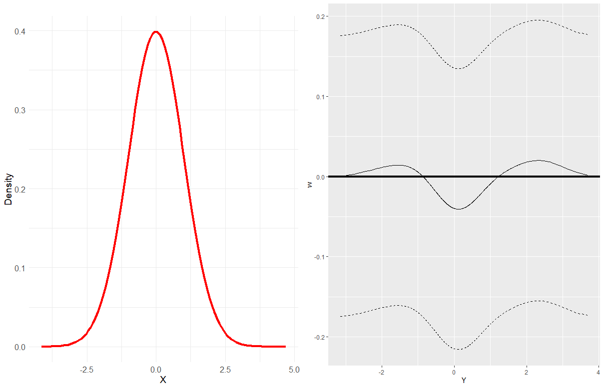
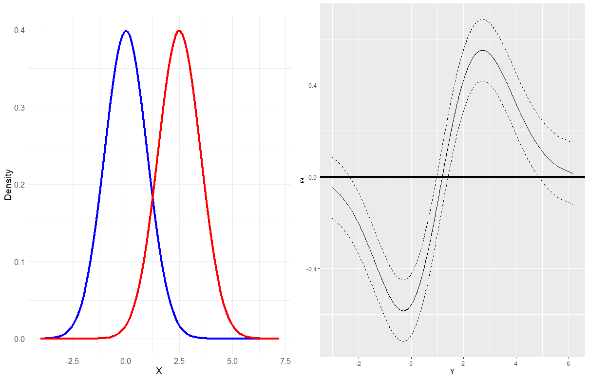
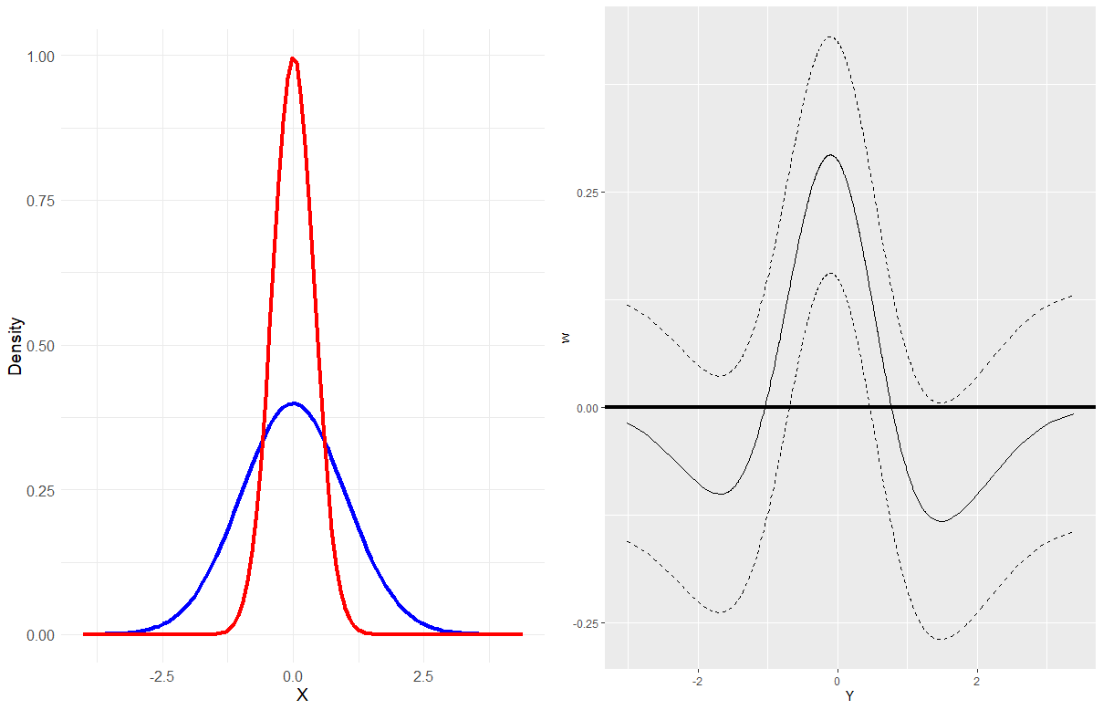
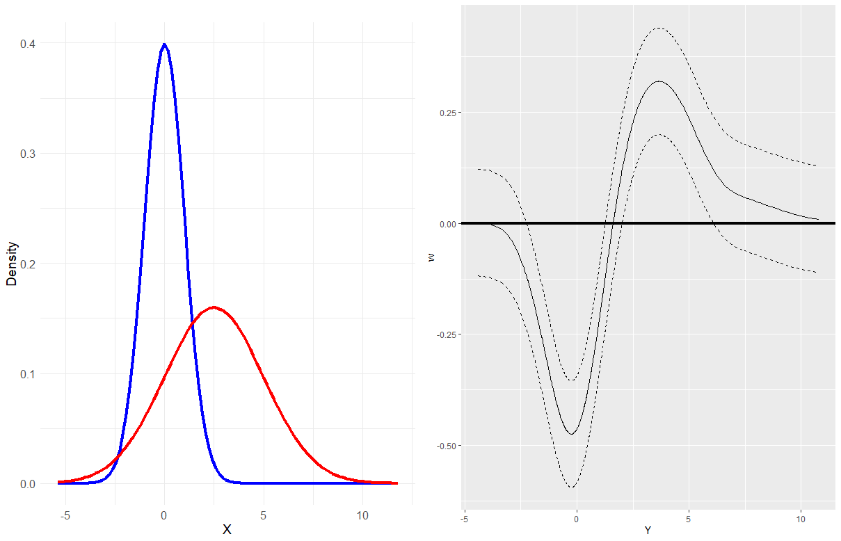
Figures 1 and 2 show both the true underlying conditional densities as well as our estimation method with confidence bands. As mentioned above, the estimated witness functions follow the difference in densities between the treatment group in red and the control group in blue. When the difference in densities is negative at $\mathbf{y}$, the value of the estimated witness function tends to be negative, and vice-versa. In particular, negative values indicate that it is less likely to observe an outcome from the treatment population at $\mathbf{y}$. Thus the witness function maps out the behavior of the treatment effect for fixed $\mathbf{x}$. As the additional confidence bands are simultaneously valid for all $y$, any crossing of zero of the lower or upper confidence bands indicates a rejection of $H_{0}\colon\mathbb{P}_{\mathbf{Y}\mkern 4.0mu{|}\mkern 4.0mu\mathbf{X}\mkern 2.5mu{=}\mkern 2.5mu\mathbf{x}}^{0}=\mathbb{P}_{\mathbf{Y}\mkern 4.0mu{|}\mkern 4.0mu\mathbf{X}\mkern 2.5mu{=}\mkern 2.5mu\mathbf{x}}^{1}$. In the left graph in Figure 1 the upper and lower confidence bands are far from zero, indicating that the method recognizes that there is no effect. For all other examples, Causal-DRF indicates correctly that there is a significant effect, as in each example the confidence bands have regions that do not intersect zero. Even in challenging cases such as Example 3, where there is only a variance shift, Figure 2 shows a clear rejection of $H_{0}$.

These examples indicate how the CKTE, estimated through Causal-DRF, can give a clearer picture of conditional treatment effects that go beyond differences in expectation. Moreover, the confidence bands offer a convenient tool to assess whether the effect is statistically significant. We note that the analysis for the last two cases is quite different if only the CATE is considered. First, the CATE will miss the decrease in variance in the second example. Second, while the last example may appear to be a success when only expectations are considered, only examining CATE will lead to missing differing variances in the treatment and control groups.

We start by reviewing the core DRF algorithm; for a full treatment, see Ćevid et al. (2022) and Näf et al. (2023). The DRF estimate of the CME can be viewed as a weighted average over the training points. These weights $\hat{w}_{i}(\mathbf{x})$ are found by fitting a random forest type algorithm within the RKHS $({\mathcal{H}},k)$. Specifically, a forest of $N$ trees is constructed. Each tree recursively splits the observations into sets $\mathcal{I}_{L}=\{i:X_{ij}<c\}$ and $\mathcal{I}_{R}=\{i:X_{ij}\geq c\}$, with a splitting value $c\in\mathbb{R}$ and a splitting feature $j$ chosen by a splitting criterion that is allowed to depend on $\mathbf{Y}$. In the original DRF algorithm, the Maximum Mean Discrepancy (MMD) statistic (Gretton et al., 2007) is used as a splitting criterion. This choice of splitting criterion can be interpreted as an analogue of the traditional CART splitting criterion (Breiman, 2001), but rather applied in the RKHS. Combining this idea with principles of forest construction developed by Wager and Athey (2018); Athey et al. (2019), we develop a novel splitting criterion in the RKHS that can be used to estimate $\tau_{k}(\mathbf{x})$. That is, if for a given node, the estimate in the left child, is given as

and similarly with $\hat{\tau}_{R}$, then we split such that a weighted version of

is maximal. This is a weighted version of the MMD statistic used in Ćevid et al. (2022), with weights

and similarly for $\nu_{i,R}$. Thus, using the same random approximation as in Ćevid et al. (2022) for a translation-invariant kernel (see (K3) below) this can be efficiently approximated using $S$ random functionals. For a set of candidate variables, ${\mathcal{I}}_{l}$, ${\mathcal{I}}_{R}$ are chosen to maximize this criterion. Details are given in Appendix A.

For each fitted tree $l=1,\ldots,N$, let $\mathcal{L}(\mathbf{x})$ be the leaf node of $\mathbf{x}$. The estimate of $\tau_{k}(\mathbf{x})$ is then an average over the $N$ trees,

This approach has the same computational complexity of the original DRF algorithm, specifically $\mathcal{O}(S\times N\times p\times n\log n)$; see Ćevid et al. (2022). Collecting all $k(\mathbf{Y}_{j},\cdot)$, one can rewrite $\hat{\tau}_{n,k}(\mathbf{x})$ more conveniently as

with

Finally, to allow for the construction of tests and confidence bands, we consider the following half-sampling approach similar to that of Näf et al. (2023). For a subset ${\mathcal{S}}\subset\{1,\ldots,n\}$, denote by $\hat{\tau}_{n,k}^{{\mathcal{S}}}(\mathbf{x})$ the version of $\hat{\tau}_{n,k}(\mathbf{x})$ that uses trees built with data from ${\mathcal{S}}$. We draw ${\mathcal{S}}$ by sampling $n$ i.i.d. random variables $U_{i}\sim\mathrm{Bernoulli}(1/2)$ and set ${\mathcal{S}}=\{i\colon U_{i}=1\}$. Note that $|{\mathcal{S}}|/n\to 1/2$ almost surely. Thus, we fit $B$ subforests with $L$ trees, such that $N=B*L$. The resulting estimates $\hat{\tau}_{n,k}^{{\mathcal{S}}_{b}}(\mathbf{x})$, $b=1,\ldots,B$, correspond to an approximation of the sampling distribution of $\hat{\tau}_{n,k}(\mathbf{x})$; we formalize this notion in the following section. The point estimate of the CME is then calculated by averaging the point predictions over all the half-samples:

which corresponds to (3). Algorithms 1 and 2 provide pseudocode for this procedure. This approach again has the same complexity as one fit of DRF (Ćevid et al., 2022), except that $N=B*L$ should be chosen quite large.

The Causal-DRF estimator can be conveniently written in matrix form. Consider the matrix $\mathbf{K}=(k(\mathbf{Y}_{i},\mathbf{Y}_{j}))_{i=1,\ldots n,j=1,\ldots n}$. Denote by $\hat{\mathbf{w}}\in\mathbb{R}^{n}$ the vector that concatenates the weights in (4) and similarly let $\hat{\mathbf{w}}^{{\mathcal{S}}_{b}}\in\mathbb{R}^{n}$ be the weights of the $b$th subforest. Let $\mathbf{k}=(k(\mathbf{Y}_{1},\cdot),\ldots,k(\mathbf{Y}_{n},\cdot))^{\top}$, and denote by $\mathbf{k}(\mathbf{y})=(k(\mathbf{Y}_{1},\mathbf{y}),\ldots,k(\mathbf{Y}_{n},\mathbf{y}))^{\top}$ for $\mathbf{y}\in\mathbb{R}^{d}$. Then,

Next, we show how to construct tests and confidence bands. Following the software implementation, we will take $k$ to be the Gaussian kernel given by

Note that with this choice, it holds that $\sup_{\mathbf{y},\mathbf{y}^{\prime}}k(\mathbf{y},\mathbf{y}^{\prime})\leq 1$. In practive, we follow Ćevid et al. (2022); Näf et al. (2023) and choose $\sigma^{2}$ using the median heuristic of Gretton et al. (2012).

To calculate tests and confidence bands for $\hat{\tau}_{n,k}(\mathbf{x})$, we first compute $q_{n,\alpha}$, the $1-\alpha$ quantile of the $B$ many draws from

Then a test for $H_{0}\colon\mathbb{P}_{\mathbf{Y}\mkern 4.0mu{|}\mkern 4.0mu\mathbf{X}\mkern 2.5mu{=}\mkern 2.5mu\mathbf{x}}^{0}=\mathbb{P}_{\mathbf{Y}\mkern 4.0mu{|}\mkern 4.0mu\mathbf{X}\mkern 2.5mu{=}\mkern 2.5mu\mathbf{x}}^{1}$ can be constructed as

while a simultaneous $1-\alpha$ confidence band around $\hat{\tau}_{n,k}(\mathbf{x})$ can be constructed as:

In the next section we prove consistency and asymptotic normality of $\hat{\tau}_{n,k}(\mathbf{x})$, that $\phi$ is an asymptotically valid test and that $\mathcal{B}(\mathbf{y})$ provides asymptotically uniform coverage over $\mathbf{y}\in\mathbb{R}^{d}$.

In this section we establish theoretical guarantees for the Causal-DRF algorithm, including its consistency and asymptotic normality. Notably, we are able to establish similar guarantees as Näf et al. (2023), who rely on fitting separate forests for the treatment and control groups.

For convenience, denote the kernel embeddings as $\mu^{(j)}(\mathbf{x})=\mathbb{E}[k(\mathbf{Y}^{j},\cdot)\mkern 4.0mu{|}\mkern 4.0mu\mathbf{X}\mkern 2.5mu{=}\mkern 2.5mu\mathbf{x}]$, for $j\in\{0,1\}$ and $\mu(\mathbf{x})=\mathbb{E}[k(\mathbf{Y},\cdot)\mkern 4.0mu{|}\mkern 4.0mu\mathbf{X}\mkern 2.5mu{=}\mkern 2.5mu\mathbf{x}]$. To begin, we assume the forest satisfies Assumptions (F1)–(F6) and (F1enumi) in Appendix B.1. These assumptions are a combination and refinement of the assumptions taken in Wager and Athey (2018) and Näf et al. (2023). In addition, we place the following assumptions on the data-generating process.

1. (D1)

   The covariates $\mathbf{X}_{1},\ldots,\mathbf{X}_{n}$ are i.i.d. on $[0,1]^{p}$, and admit a density that is bounded away from $0$ and infinity.

2. (D2)

   The mappings $\mathbf{x}\mapsto\mu^{(j)}(\mathbf{x})$ are Lipschitz for $j\in\{0,1\}$.

3. (D3)

   $\mathrm{Var}(k(\mathbf{Y}^{j},\cdot)\mkern 4.0mu{|}\mkern 4.0mu\mathbf{X}=\mathbf{x})=\mathbb{E}[\|k(\mathbf{Y}^{j},\cdot)\|_{{\mathcal{H}}}^{2}\mkern 4.0mu{|}\mkern 4.0mu\mathbf{X}=\mathbf{x}]-\|\mathbb{E}[k(\mathbf{Y}^{j},\cdot)\mkern 4.0mu{|}\mkern 4.0mu\mathbf{X}=\mathbf{x}]\|_{{\mathcal{H}}}^{2}>0$, for $j\in\{0,1\}$.

4. (D4)

   For all $f\in{\mathcal{H}}\setminus\{0\}$, $\mathrm{Var}(\langle k(\mathbf{Y}^{j},\cdot),f\rangle\mkern 4.0mu{|}\mkern 4.0mu\mathbf{X}=\mathbf{x})=\mathrm{Var}(f(\mathbf{Y}^{j})\mkern 4.0mu{|}\mkern 4.0mu\mathbf{X}=\mathbf{x})>0$, for $j\in\{0,1\}$.

5. (D5)

   For all $f\in{\mathcal{H}}\setminus\{0\}$, $\mathbf{x}\mapsto\mathbb{E}[\left|f(\mathbf{Y}^{j})\right|^{2}\mkern 4.0mu{|}\mkern 4.0mu\mathbf{X}=\mathbf{x}]$ is Lipschitz, for $j\in\{0,1\}$.

As noted in Näf et al. (2023, page 10), (D3) is automatically satisfied for the Gaussian kernel under the assumption that the conditional distributions $\mathbf{Y}^{j}\mkern 4.0mu{|}\mkern 4.0mu\mathbf{X}=\mathbf{x}$ for $j\in\{0,1\}$ are not point measures. We also adopt the following traditional causal assumptions.

1. (C1)

   Positivity (overlap): there exists $\varepsilon>0$ such that for all $\mathbf{x}$,

   $\displaystyle\varepsilon<\mathbb{P}(W=1\mkern 4.0mu{|}\mkern 4.0mu\mathbf{X}=\mathbf{x})<1-\varepsilon$

   (10)

2. (C2)

   Unconfoundedness (no unmeasured confounding): $(\mathbf{Y}^{0},\mathbf{Y}^{1})\mathchoice{\mathrel{\hbox to0.0pt{$\displaystyle\perp$\hss}\mkern 2.0mu{\displaystyle\perp}}}{\mathrel{\hbox to0.0pt{$\textstyle\perp$\hss}\mkern 2.0mu{\textstyle\perp}}}{\mathrel{\hbox to0.0pt{$\scriptstyle\perp$\hss}\mkern 2.0mu{\scriptstyle\perp}}}{\mathrel{\hbox to0.0pt{$\scriptscriptstyle\perp$\hss}\mkern 2.0mu{\scriptscriptstyle\perp}}}W\mkern 4.0mu{|}\mkern 4.0mu\mathbf{X}$

Finally, we place assumptions (K1)–(K4) (Appendix C) on the kernel function $k$. All of these assumptions are met by the Gaussian kernel given in (6).

References

Athey et al. (2019)
Susan Athey, Julie Tibshirani, and Stefan Wager.
Generalized random forests.
The Annals of Statistics, 47(2):1148–1178, 2019.
Bénard et al. (2024)
Clément Bénard, Jeffrey Näf, and Julie Josse.
MMD-based variable importance for distributional random forest.
In Proceedings of The 27th International Conference on
Artificial Intelligence and Statistics, volume 238, pages 1324–1332, 2024.
Benjamin (2003)
Daniel J Benjamin.
Does 401(k) eligibility increase saving?: Evidence from propensity
score subclassification.
Journal of Public Economics, 87(5):1259–1290, 2003.
Breiman (2001)
Leo Breiman.
Random forests.
Machine learning, 45(1):5–32, 2001.
Ćevid et al. (2022)
Domagoj Ćevid, Loris Michel, Jeffrey Näf, Nicolai Meinshausen, and
Peter Bühlmann.
Distributional random forests: Heterogeneity adjustment and
multivariate distributional regression.
Journal of Machine Learning Research, 23(333):1–79, 2022.
Chen and White (1998)
Xiaohong Chen and Halbert White.
Central limit and functional central limit theorems for
hilbert-valued dependent heterogeneous arrays with applications.
Econometric Theory, 14(2):260–284, 1998.
Chernozhukov and Hansen (2004)
Victor Chernozhukov and Christian Hansen.
The Effects of 401(K) Participation on the Wealth Distribution: An
Instrumental Quantile Regression Analysis.
The Review of Economics and Statistics, 86(3):735–751, 2004.
Chernozhukov et al. (2013)
Victor Chernozhukov, Iván Fernández-Val, and Blaise Melly.
Inference on counterfactual distributions.
Econometrica, 81(6):2205–2268, 2013.
Chernozhukov et al. (2020)
Victor Chernozhukov, Iván Fernandez-Val, and Martin Weidner.
Network and panel quantile effects via distribution regression.
Journal of Econometrics, 2020.
Dudley (2002)
Richard M. Dudley.
Real Analysis and Probability.
Cambridge Studies in Advanced Mathematics. Cambridge University
Press, 2002.
Fawkes et al. (2022)
Jake Fawkes, Robert Hu, Robin J. Evans, and Dino Sejdinovic.
Doubly robust kernel statistics for testing distributional treatment
effects even under one sided overlap.
Preprint arXiv:1510.04342, 2022.
González-Rodríguez and Colubi (2017)
Gil González-Rodríguez and Ana Colubi.
On the consistency of bootstrap methods in separable Hilbert
spaces.
Econometrics and Statistics, 1:118–127, 2017.
Gretton et al. (2007)
Arthur Gretton, Karsten Borgwardt, Malte Rasch, Bernhard Schölkopf, and
Alex J. Smola.
A kernel method for the two-sample-problem.
In Advances in Neural Information Processing Systems, pages
513–520, 2007.
Gretton et al. (2012)
Arthur Gretton, Dino Sejdinovic, Heiko Strathmann, Sivaraman Balakrishnan,
Massimiliano Pontil, Kenji Fukumizu, and Bharath K. Sriperumbudur.
Optimal kernel choice for large-scale two-sample tests.
1205–1213, 2012.
Hohberg et al. (2020)
Maike Hohberg, Peter Pütz, and Thomas Kneib.
Treatment effects beyond the mean using distributional regression:
Methods and guidance.
PLOS ONE, 15(2):1–29, 02 2020.
Hsing and Eubank (2015)
Tailen Hsing and Randall Eubank.
Theoretical Foundations of Functional Data Analysis, with an
Introduction to Linear Operators.
Wiley Series in Probability and Statistics. Wiley, 2015.
Kallus and Oprescu (2023)
Nathan Kallus and Miruna Oprescu.
Robust and agnostic learning of conditional distributional treatment
effects.
In Proceedings of The 26th International Conference on
Artificial Intelligence and Statistics, volume 206, pages 6037–6060, 2023.
Kosorok (2008)
Michael R. Kosorok.
Introduction to Empirical Processes and Semiparametric
Inference.
Springer Series in Statistics. Springer New York, 2008.
Martinez Taboada et al. (2023)
Diego Martinez Taboada, Aaditya Ramdas, and Edward Kennedy.
An efficient doubly-robust test for the kernel treatment effect.
In Advances in Neural Information Processing Systems,
volume 36, pages 59924–59952, 2023.
Muandet et al. (2021)
Krikamol Muandet, Motonobu Kanagawa, Sorawit Saengkyongam, and Sanparith
Marukatat.
Counterfactual mean embeddings.
Journal of Machine Learning Research, 22(162):1–71, 2021.
Näf et al. (2023)
Jeffrey Näf, Corinne Emmenegger, Peter Bühlmann, and Nicolai Meinshausen.
Confidence and uncertainty assessment for distributional random
forests.
Journal of Machine Learning Research, 24(366):1–77, 2023.
Park et al. (2021)
Junhyung Park, Uri Shalit, Bernhard Schölkopf, and Krikamol Muandet.
Conditional distributional treatment effect with kernel conditional
mean embeddings and U-statistic regression.
In Proceedings of 38th International Conference on Machine
Learning (ICML), volume 139, pages 8401–8412, 2021.
Pisier (2016)
Gilles Pisier.
Martingales in Banach Spaces.
Press, 2016.
Rahimi and Recht (2008)
Ali Rahimi and Benjamin Recht.
Random features for large-scale kernel machines.
1177–1184, 2008.
Rubin (2005)
Donald B Rubin.
Causal inference using potential outcomes.
Journal of the American Statistical Association, 100(469):322–331, 2005.
Simon-Gabriel et al. (2023)
Carl-Johann Simon-Gabriel, Alessandro Barp, Bernhard Schölkopf, and Lester
Mackey.
Metrizing weak convergence with maximum mean discrepancies.
Journal of Machine Learning Research, 24(184):1–20, 2023.
Sriperumbudur (2016)
Bharath Sriperumbudur.
On the optimal estimation of probability measures in weak and strong
topologies.
Bernoulli, 22(3):1839–1893, 2016.
Umegaki and Bharucha-Reid (1970)
Hisaharu Umegaki and A.T Bharucha-Reid.
Banach space-valued random variables and tensor products of banach
Journal of Mathematical Analysis and Applications, 31(1):49–67, 1970.
Wager and Athey (2017)
Stefan Wager and Susan Athey.
Estimation and inference of heterogeneous treatment effects using
random forests.
Preprint arXiv:1510.04342, 2017.
Wager and Athey (2018)
Journal of the American Statistical Association, 113(523):1228–1242, 2018.
Wendland (2004)
Holger Wendland.
Scattered Data Approximation.
Cambridge Monographs on Applied and Computational Mathematics.
Cambridge University Press, 2004.
doi: 10.1017/CBO9780511617539.
Zhao and Meng (2015)
Ji Zhao and Deyu Meng.
FastMMD: Ensemble of circular discrepancy for efficient two-sample
test.
Neural computation, 27(6):1345–1372,
2015.
Appendix A Details on the Splitting Criterion
Following Ćevid et al. (2022), we adopt an approximate kernel that is a fast random approximation of the MMD statistic (Zhao and Meng, 2015). Such an approximation allows for the computational efficiency necessary to allow the number of kernel computations that are required when constructing a large forest.
By Bochner’s theorem (see e.g. Wendland (2004, Theorem 6.6)), any bounded shift-invariant kernel can be written as
(26)
This can be interpreted as a Fourier transform of some measure . By randomly sampling the frequency vectors from normalized , we can approximate our kernel up to a scaling factor by the approximate kernel via:
where is the kernel function with the feature map given by
a random vector of the Fourier features (Rahimi and Recht, 2008).
Our default choice of kernel is the
the Gaussian kernel with bandwidth , as there is a straightforward expression for . We can then sample . The bandwidth is chosen as the median pairwise distance between all training responses (the ’median heuristic’; Gretton et al.2012).
Our splitting criterion seeks to maximize
(27)
which is a weighted version of the MMD statistic used in Ćevid et al. (2022), with weights
and similarly . Using the approximate in (A) results in:
(28)
which is the splitting criterion used in the forest.
Appendix B Preliminaries
The following assumptions are placed on the choice of kernel.
(K1)
is bounded, i.e., .
(K2)
is (jointly) continuous.
(K3)
The kernel is translation-invariant, i.e. for some function .
(K4)
is integrally strictly positive definite (denoted by spd), that is
see for instance Sriperumbudur (2016); Simon-Gabriel et al. (2023).
The forest assumptions with a refinement are discussed below in Section B.1.
First, we reproduce notation, definitions, and elementary results from (Näf et al., 2023).
Let denote the underlying probability space.
Throughout, let denote the RKHS associated with the kernel .
We assume that is bounded and continuous in its two arguments. Boundedness of ensures that is indeed defined on all of , and continuity of ensures that is separable. Thus, we assume throughout that (K2) holds, such that measurability issues can be avoided. Let us denote by a map from to . Separability implies that such a map
is measurable if and only if is measurable for all .
Moreover, it can easily be checked that is linear on . Separability of and mean that the integral
is well defined and that
for any continuous linear function .111Here and below, is meant to denote for all . In particular, for all . Moreover, for , denote by
Furthermore, it is well-known that is a Banach space with
This allows us to
also define conditional expectations. For a sub -algebra and an element , the conditional expectation is the (a.s.) unique element such that
(CE1)
is measurable and ,
(CE2)
for all ;
see for instance Umegaki and Bharucha-Reid (1970) or Pisier (2016, Chapter 1).
Particularly, condition (C2) implies that due to for any -algebra. It can also be shown that for all linear and continuous and that (Pisier, 2016, Chapter 1). Moreover, it can be shown that
(CE3)
For , is the orthogonal projection onto ;
see (Umegaki and Bharucha-Reid, 1970).
Although the conditional expectation , similarly to real-valued conditional expectations, is only defined a.s., we do not explicitly state this in our developments below. Denote
. Proposition 6 and 7 in Ćevid et al. (2022) show that this notion is well-defined and establishes further properties of Hilbert space-valued conditional expectations.
For two functions and with , we denote
if
for some . If , we write . For a sequence of random variables and a sequence of real numbers , , we write if
that is, is bounded in probability. We write if converges to zero in probability. Similarly, for a separable metric space, , and measurable, we write , if . By separability, every random element with values in is tight (Dudley, 2002, Chapter 7.1). That is, for all , there is a compact such that . More generally, uniform tightness of a sequence , means that for all , there is a compact such that
Finally, let and , and assume that depends on , . Thus, for fixed to a certain value, is a fixed set. If almost everywhere, we define
Then, we have by construction that
(29)
For a more compact notation in the following Lemma, let , and let for and , let be the set of all subsets of size drawn from without replacement, with . The following lemma presents a U-statistic expansion that we afterwards apply to an individual tree of our DRF forest.
Let and be two separable Hilbert spaces, and let be i.i.d. copies of a random element . Write , and let measurable with
. If is symmetric, there exist functions , , such that
(30)
and it holds that
(31)
and
B.1 Forest Assumptions and a Refinment
We first list the forest assumptions taken in Wager and Athey (2018):
(F1)
(Honesty) The data used for constructing each tree is split into two halves; the first is used for determining the splits and the second for populating the leaves and thus for estimating the response. In addition, from the second sample may be used to define the splits.
(F2)
(Random-split) At every split point and for all feature dimensions , the probability that the split occurs along the feature is bounded from below by for some .
(F3)
(Symmetry) The (randomized) output of a tree does not depend on the ordering of the training samples.
(F4)
(-regularity)
For the second sample in (F1), after splitting a parent node, each child node contains at least a fraction of the parent’s training samples. Moreover, the trees are grown until every leaf contains between and many observations from each treatment group, for some fixed tuning parameter .
(F5)
(Data sampling)
To grow a tree, a subsample of size out of the training data points is sampled.
We consider with
These conditions can be ensured by forest construction, although, as mentioned in Wager and Athey (2018), care must be taken for different test points , as (F4) must be ensured for each test point.
In the following, denote the indices of the first sample used to build the trees in (F1) as , and the second sample used to populate the leaves as . Näf et al. (2023) assumed the equivalent of (F1)–(F5) to derive analogous results for DRF. Unfortunately, a crucial proof in Näf et al. (2023), corresponding to Theorem 9 below, only goes through under the assumption that for each , is independent of , the leaf falls into. However, while this is approximately true, since an independent sample is used for each tree to build , there can be a certain dependence, as might be adjusted to ensure (F4). That is, while a first is built completely independently of from the second sample, is then adjusted based on from the second sample to meet (F4). Although the nature of this dependence is hard to control, we now put some mild assumptions to limit the dependence between and in any forest construction meeting (F1)–(F5). In particular, we assume:
(F1enumi)
(Honesty*) The second sample is used such that: for all , for all bounded,
(32)
(33)
for some .
Finally, for Causal-DRF we in addition need an assumption of the behavior of the weight in each class:
(F6)
(Group Variance)
There exists some , such that for all ,
(34)
Remark 2
Both Assumption (F1enumi) and (F6) are needed to prove Theorem 9, which considers the asymptotic ratio of variances of the projected trees:
With (32), we assume that the adaptation of by , is done in such a way that the dependence is negligible for each individual . Intuitively, one might expect this variance to be , even if the second sample was freely used to build , as is one of points used to obtain . The additional encodes that is originally build from an independent set of observations and , is only used to adapt such that (F4) holds. Similarly, ((F1enumi)) demands that, given and , the dependence of on all other observations be negligible. Although are independent, conditioning on and will induce (conditional) dependence in general. With ((F1enumi)) we assume that this dependence decreases sufficiently fast as .
As we are only interested in the ratio of variances with identical trees, the denominator and numerator deal with the same dependence of on . Thus, it might be possible to further weaken assumption (F1enumi). However, (F1enumi) is much more plausible for a forest construction satisfying (F1)–(F5) than the full independence of and the second sample implicitly assumed by Näf et al. (2023). Both assumptions (without ) are also needed for the original DRF, as we discuss in a correction of a key proof argument of Näf et al. (2023) in Section B.2.
Assumption (F6) is the same as Assumption (30) in Näf et al. (2023), ensuring the convergence of the ratio by restricting how the variances can behave in each group. Without it can be shown that there exists constants , such that
(F6) is a sufficient condition that ensures that the ratio does not indefinitely fluctuate between these values as .
However, following Wager and Athey (2018) and Näf et al. (2023) we only acknowledge the sample splitting in the tree when it is necessary, such as in the proof of Theorem 9.
Before we continue with the main proofs, it is instructive to present the corrected argument of a crucial part of the proof of Theorem 5 in Näf et al. (2023). These arguments can then directly be reused to obtain important claims to ultimately proof Theorem 9 below.
B.2 Improving upon the proof of Theorem 5 in Näf et al. (2023)
We restate here the assumptions of Näf et al. (2023): We refer here to the assumptions (F1)–(F5) from Näf et al. (2023) as (DRF-F1)–(DRF-F5). These are essentially the assumptions (F1)–(F5) shown here when is seen as part of . We repeat here the assumptions on the data taken in Näf et al. (2023):
(DRF-D1)
The covariates are independent and identically distributed on with a density bounded away from and infinity.
(DRF-D2)
The mapping is Lipschitz.
(DRF-D3)
(DRF-D4)
.
(DRF-D5)
, for some constants uniformly over .
(DRF-D6)
For all , .
(DRF-D7)
For all , is Lipschitz.
Instead of demanding (finite-sample) independence, we ask that the dependence between , and the leaf decays at a certain rate, namely:
(DRF-F1enumi)
(35)
(36)
With (35), we assume that the adaptation of by , is done in such a way that the dependence is negligible for each individual . Intuitively we might expect this variance to be , even if the second sample was freely used to build , as is one of points used to obtain . The additional encodes that is originally build from an independent set of observations and , is only used to adapt such that (F4) holds. This is a convenient and mild assumption that allows for an elegant correction of the proof in Näf et al. (2023), although it might be possible to weaken it.
This assumption holds in particular, if is independent of , .
Similarly ((DRF-F1enumi)) is a mild assumption that holds in particular in the following: Assume the sample in is used to adapt an original build from independent data in , based solely on whether , as for instance shown in Figure 6. Then it holds that,
(37)
Thus in this plausible scenario, a condition much stronger than ((DRF-F1enumi)) holds.
Figure 6: Potential Tree building approach for that satisfies ((DRF-F1enumi)). Crucially, is an adapted version of based only on whether , is included in .
To establish the setting of Näf et al. (2023), define in the following the number of data points belonging to the same leaf as as and let
(38)
be the weight associated with each observation in a tree with integrated out, i.e. , such that
We will make use the following property of the :
(39)
In particular,
(40)
We define
(41)
(42)
so that
. We now formulate the corrected version of Theorem 5 in Näf et al. (2023) with (DRF-F1enumi) added:
We note that takes the sum over all possible subsets of size . As such, the chosen subsets of size might not have the indices in general. To simplify notation we usually only consider the indices , appealing to the assumption of i.i.d. data.
Lemma 5
Suppose (D1) holds for and (F3), (F4) for . Moreover, assume (C1) holds. Then, there is a constant depending on and such that,
(73)
where is from the overlap condition in (C1). When is uniform over , the bound holds with . Moreover, it holds that for
(74)
Proof
The proof of (73) is the same as in Wager and Athey (2017, p. 47) when proving incrementally.
We next note that for
and that by (F4), is not empty, for . Thus indeed , so that . Thus it follows by the i.i.d assumption that
showing . Since , this also shows that . By the overlap conditon (C1), we moreover have:
showing that as well.
Finally, using the fact that ,
and similarly for .
We note that by honesty (F1), , and so the same properties also hold, for , in particular
(75)
This also implies that
(76)
With (75), this means that the difference between and is negligible. Let
This helps to relate the behavior of to the overall variance . In particular, either or or both. These arguments will be crucial for the proof of Theorem 9 below. We now turn to the behavior of the bias:
Lemma 6
Assume (F2)–(F4)
that is trained on data . Suppose that assumption (D1) holds for and that (C1) holds. Then,
(80)
This follows directly from the arguments in Wager and Athey (2017, pages 34 and 46), in addition to a union bound over all dimensions of . In particular, instead of we need to consider the minimal number of observations of the smaller class receives, say . By (C1), it holds a.s. that , such that can be replaced by .
Corollary 7
In addition to the conditions of Lemma 6, assume (D2), (C2) and that the trees in the forest satisfy (F1). Then, we have
Adapting the arguments of Ćevid et al. (2022, Lemma 12), using that ,
where the last argument follows by (C2). The same applies to the control group, and with (D2) thus we can directly apply the arguments in Ćevid et al. (2022, Corollary 13) for each term separately to obtain
Since the bias of a tree is the same as the bias of the overall forest, we obtain (81).
Denote by
(82)
and by
(83)
the first order approximation of as in Lemma 1. Recall from the main text that and . Moreover, we define the random element
In the following, we give our crucial result, Theorem 9, which studies the behavior of , for any , and . In particular Theorem 9 implies that:
1.
The ratio of to converges to a real number under (F6). This will be crucial in showing univariate convergence, which in turn is a crucial ingredient in showing total convergence.
2.
Together with Lemma 5, (75) and (C), it shows that
(90)
This will be essential, as it means that the variance of the first-order approximation decays slow enough relative to the variance of the actual tree .
Remark 8
The reason certain proofs are more difficult here than for the original DRF in Näf et al. (2023), is that now conditioning on means also conditioning on . Thus, compared to DRF for Causal-DRF we need to differentiate the case and . Although this may seem benign, it requires a more careful treatment.
Throughout we focus on proving (9) for , as the proof for works analogously.
By the same arguments as in Näf et al. (2023, Theorem 5) and Wager and Athey (2017), we can ignore the double-sampling aspect in (F1) and condition on a point used in populating the trees (i.e. ) and use rather than elements in the tree predictions to simplify notation.
Recall that , such that,
Let , and
Crucially, is chosen such that
(93)
following from Lemma 6, similar to Wager and Athey (2017).
First, using the fact that conditional expectations are projections in , we can write
(94)
as in Näf et al. (2023, Claim (69)). We start by focusing on the second variance in this sum:
Claim:
(95)
Proof: We adapt the expansion of Näf et al. (2023): By honesty (i) is independent of conditional on , and more generally, (ii) is independent of , , conditional on . Thus, using (i), (ii), and the independence of from , , we have
Note that by the Lipschitz assumption on , , i.e., (D2), it holds that
(97)
Then
(98)
For the second variance we have:
where we used assumption (D2) for the second inequality and where the last step followed because , for by definition of . Finally, because by Lemma 5, we have that
(99)
Similarly, for the covariance, it holds that
(100)
where the second last step followed because
by the boundedness of (K1). Combining (C), (99) and (C), we obtain
(101)
Focussing on the first term, we have:
(102)
For the second part, note that because and are bounded by (K2), it holds that
Finally, we consider the covariances between and :
Claim: For some ,
(140)
Proof:
Similar to above, we first simplify the expression:
Claim: For some , we have
(141)
Proof: It holds that:
We now use the Cauchy-Schwarz inequality to bound the first two covariances by the product of the square root of the variances of the respective terms. For (C1), as is bounded (K1),
Proof: This can be proven in exactly the same way as Claim (85) in Theorem 24 of Näf et al. (2023) with the regression trees , exchanged by the causal trees , .
Thus, as , combining (157) and (158), we arrive at (9).
We recall that , by Lemma 5 and thus the terms can be ignored. This together with assumption (F6) establishes (92).
Having established these basics, we can show asymptotic normality of the estimator in .
Proof: We first note that by boundedness of the kernel, for all , for some . Second, as a consequence of Theorem 9, Lemma 5, (75) and (C), (90) holds, that is:
Thus it follows that:
(161)
The same steps as in Näf et al. (2023, Theorem 3) in turn implies that
the latter going to zero as , with by (F5).222We note that Näf et al. (2023) uses the abbreviation . By Theorem 7, we also have that
Claim (159) is the first key to show asymptotic normality, as it shows that is asymptotically equivalent to a sum of independent elements in the Hilbert space . Thus we can use CLT results for , and in particular, we will show (I) marginal convergence and (II) uniform tightness:
Claim: (I) For all ,
(162)
For , consider the univariate marginal . Assumptions (F1)–(F5), (C1)–(C2) and Assumptions (D1)–(D5) verify all assumptions of Theorem 11 of Wager and Athey (2017). Consequently, there exists a converging to zero with such that
(163)
Unfortunately, the scaling factor
obtained from Wager and Athey (2018) depends on . However, from Theorem 9, it follows that
which is finite and strictly larger zero by (D3), (D4). Thus
proving the claim.
Before continuing, by the definition of , we define
Claim: (II) is uniformly tight.
Proof: Because is separable due to our assumptions on the kernel, there exists a complete orthogonal basis of ; see for instance Hsing and Eubank (2015). Let be the projection operator onto the linear span of the first elements of , . Given the tools from above, we can use the exact same arguments as in Näf et al. (2023, Theorem 6) to verify the condition , as , which is sufficient for tightness (Chen and White, 1998, Lemma 3.2).
Univariate convergence together with tightness imply ; see for example Chen and White (1998, Lemma 3.1/3.2) or Hsing and Eubank (2015, Chapter 7). Since by Equation (159) we have
the result follows.
Finally, having obtained these prior results Theorems 4, 4 and 4 can be proven using the same approach as in Näf et al. (2023) and the proofs are thus omitted.