跳到论文正文
W Papers独立论文阅读器 arXiv:2410.17405 论文正文 计算阅读时间 · 0%
引用这篇论文根据当前论文元数据生成,正式投稿前建议核对。


\newsiamremark

remarkRemark \newsiamremarkhypothesisHypothesis \newsiamthmclaimClaim \newsiamthmexampleExample \headersBenjamin-Ono Small Dispersion LimitE. Blackstone, L. Gassot, P. Gérard, and P. D. Miller \externaldocumentex_supplement

The Benjamin-Ono equation in the zero-dispersion limit for rational initial data: generation of dispersive shock waves

Elliot Blackstone Department of Mathematics, University of Michigan, Ann Arbor, MI (). eblackst@umich.edu    Louise Gassot CNRS and Department of Mathematics, University of Rennes, Rennes, France (). louise.gassot@cnrs.fr    Patrick Gérard Laboratoire de Mathématiques d’Orsay, Université Paris-Saclay, Orsay, France (). patrick.gerard@universite-paris-saclay.fr    Peter D. Miller Department of Mathematics, University of Michigan, Ann Arbor, MI (). millerpd@umich.edu
Abstract

The leading-order asymptotic behavior of the solution of the Cauchy initial-value problem for the Benjamin-Ono equation in L2​(ℝ)superscript𝐿2ℝL^{2}(\mathbb{R}) is obtained explicitly for generic rational initial data u0subscript𝑢0u_{0}. An explicit asymptotic wave profile uZD​(t,x;ϵ)superscript𝑢ZD𝑡𝑥italic-ϵu^{\mathrm{ZD}}(t,x;\epsilon) is given, in terms of the branches of the multivalued solution of the inviscid Burgers equation with initial data u0subscript𝑢0u_{0}, such that the solution u​(t,x;ϵ)𝑢𝑡𝑥italic-ϵu(t,x;\epsilon) of the Benjamin-Ono equation with dispersion parameter ϵ>0italic-ϵ0\epsilon>0 and initial data u0subscript𝑢0u_{0} satisfies u​(t,x;ϵ)−uZD​(t,x;ϵ)→0→𝑢𝑡𝑥italic-ϵsuperscript𝑢ZD𝑡𝑥italic-ϵ0u(t,x;\epsilon)-u^{\mathrm{ZD}}(t,x;\epsilon)\to 0 in the locally uniform sense as ϵ→0→italic-ϵ0\epsilon\to 0, provided a discriminant inequality holds implying that certain caustic curves in the (t,x)𝑡𝑥(t,x)-plane are avoided. In some cases this convergence implies strong L2​(ℝ)superscript𝐿2ℝL^{2}(\mathbb{R}) convergence. The asymptotic profile uZD​(t,x;ϵ)superscript𝑢ZD𝑡𝑥italic-ϵu^{\mathrm{ZD}}(t,x;\epsilon) is consistent with the modulated multi-phase wave solutions described by Dobrokhotov and Krichever.

keywords:
Benjamin-Ono equation, zero-dispersion limit, steepest descent integration.
{AMS}

35C20, 35Q51, 41A60.

1 Introduction

1.1 Background: weak dispersion and dispersive shock waves

Weakly dispersive perturbations of the initial-value problem for the inviscid Burgers equation

(1) utB+2​uB​uxB=0,uB​(0,x)=u0​(x),formulae-sequencesubscriptsuperscript𝑢B𝑡2superscript𝑢Bsubscriptsuperscript𝑢B𝑥0superscript𝑢B0𝑥subscript𝑢0𝑥u^{\mathrm{B}}_{t}+2u^{\mathrm{B}}u^{\mathrm{B}}_{x}=0,\quad u^{\mathrm{B}}(0,x)=u_{0}(x),

have been studied for many years. Their theory is complementary to that of weakly diffusive perturbations such as the well-known viscous Burgers equation ut+2​u​ux−ϵ​ux​x=0subscript𝑢𝑡2𝑢subscript𝑢𝑥italic-ϵsubscript𝑢𝑥𝑥0u_{t}+2uu_{x}-\epsilon u_{xx}=0, ϵ>0italic-ϵ0\epsilon>0, that are understood in some generality to lead to viscous shock waves converging as ϵ→0→italic-ϵ0\epsilon\to 0 in a suitable weak topology to weak solutions of (1) satisfying appropriate entropy conditions. See [8, Section 8] for an accessible review. When the perturbing terms are dispersive rather than diffusive, the perturbed system reacts to exploding gradients, a phenomenon occurring generally in solutions of (1) in finite time, by generating rapid oscillations rather than a sharp shock profile modeled as ϵ→0→italic-ϵ0\epsilon\to 0 by a traveling jump discontinuity. The field of rapid oscillations that resolve the gradient catastrophe in the solution of (1) is called a dispersive shock wave.

At a formal level, the oscillations making up the dispersive shock wave can be studied using the wave modulation theory of Whitham [37]. Whitham’s theory starts with a family of exact periodic traveling wave solutions of the dispersive model indexed by constant parameters such as the wavenumber, frequency, and amplitude of the wave. Subject to an ansatz of a solution fitting this form but with constant parameters replaced by slowly-varying functions instead, the theory predicts a system of modulation equations governing the wave parameters. There are several approaches to deriving the modulation equations going back to the early work of Whitham; for instance one can average the densities and fluxes in a sufficient number of local conservation laws [36], or equivalently one can average the density of a Lagrangian [35] and obtain the modulation equations from an averaged variational principle. This theory requires rather few assumptions about the dispersive perturbation of (1) and applies also to weakly-dispersive perturbations of more complicated quasilinear systems. See [15] and [5] for an up-to-date review.

While there is no specific reason to doubt its validity, the Whitham theory has only been rigorously established in isolated cases, usually with proofs relying on complete integrability. The most famous completely integrable dispersive perturbation of the inviscid Burgers initial-value problem (1) is that of the Korteweg-de Vries equation

(2) ut+2​u​ux+ϵ2​ux​x​x=0.subscript𝑢𝑡2𝑢subscript𝑢𝑥superscriptitalic-ϵ2subscript𝑢𝑥𝑥𝑥0u_{t}+2uu_{x}+\epsilon^{2}u_{xxx}=0.

In some sense, it was the formation of dispersive shock waves that led to the discovery of complete integrability for certain nonlinear dispersive wave equations. Indeed, in the famous paper of Zabusky and Kruskal [38], the Korteweg-de Vries initial-value problem was solved numerically with sinusoidal initial data and a small value of ϵitalic-ϵ\epsilon, and the individual peaks of the dispersive shock wave were identified for the first time as “solitons”. There were also hints that the Whitham theory for the Korteweg-de Vries equation had special properties, going back to the nontrivial observation of Whitham [36] that the 3×3333\times 3 quasilinear first-order system of modulation equations was not only hyperbolic but also admitted a complete set of independent Riemann invariants. Also, the periodic traveling wave solutions on which the Whitham theory is based were generalized in the Korteweg-de Vries setting to multi-phase wave solutions, for which modulation equations were also obtained and shown to have the same property for reasons related to complete integrability [17]. The rigorous mathematical theory of the zero-dispersion limit ϵ→0→italic-ϵ0\epsilon\to 0 of the Korteweg-de Vries equation began with the work of Lax and Levermore [28], who established the existence of an ϵitalic-ϵ\epsilon-independent limit u¯​(t,x)¯𝑢𝑡𝑥\bar{u}(t,x) of the solution u​(t,x;ϵ)𝑢𝑡𝑥italic-ϵu(t,x;\epsilon) in the weak L2​(ℝ)superscript𝐿2ℝL^{2}(\mathbb{R}) sense for each t≥0𝑡0t\geq 0. The Lax-Levermore theory describes u¯​(t,x)¯𝑢𝑡𝑥\bar{u}(t,x) as the solution of a limiting variational problem for measures that are weak-∗∗\ast limits of discrete measures; subsequently Venakides [34] showed how the retention of the discrete nature of the measure allows one to capture the profile of the 𝒪​(ϵ)𝒪italic-ϵ\mathcal{O}(\epsilon)-wavelength oscillations of the dispersive shock wave. Venakides’ theory was not able to fully resolve the phase of the dispersive shock wave profile, but that was eventually achieved using the Riemann-Hilbert formulation of the inverse-scattering problem for the Korteweg-de Vries equation and applying the Deift-Zhou steepest descent technique [13]. Further developments towards universality properties near wave caustics were achieved by Claeys and Grava in [10, 11, 12].

1.2 The Benjamin-Ono equation

Another weakly-dispersive correction to the inviscid Burgers equation is the Benjamin-Ono equation

(3) ut+(u2)x=ϵ​∂x|Dx|​u,x∈ℝ,t≥0,ϵ>0,formulae-sequencesubscript𝑢𝑡subscriptsuperscript𝑢2𝑥italic-ϵsubscript𝑥subscript𝐷𝑥𝑢formulae-sequence𝑥ℝformulae-sequence𝑡0italic-ϵ0u_{t}+(u^{2})_{x}=\epsilon\partial_{x}|D_{x}|u,\quad x\in\mathbb{R},\quad t\geq 0,\quad\epsilon>0,

where the operator |Dx|subscript𝐷𝑥|D_{x}| can be defined via a Fourier multiplier as |Dx|​u^​(ξ)=|ξ|​u^​(ξ)^subscript𝐷𝑥𝑢𝜉𝜉^𝑢𝜉\widehat{|D_{x}|u}(\xi)=|\xi|\widehat{u}(\xi). Like the Korteweg-de Vries equation, equation (3) can be derived as an asymptotic model for long water waves of small amplitude, although for (3) these are internal waves on a free surface between two density-stratified fluids with the lower layer being infinitely deep.

Like the Korteweg-de Vries equation, the Benjamin-Ono equation is understood to be a completely integrable system, although many aspects of the corresponding theory are quite different in character. Here we restrict the discussion to the aspects that are germane to the zero-dispersion limit ϵ→0→italic-ϵ0\epsilon\to 0 for (3) posed with given initial data u​(0,x;ϵ)=u0​(x)𝑢0𝑥italic-ϵsubscript𝑢0𝑥u(0,x;\epsilon)=u_{0}(x) independent of ϵitalic-ϵ\epsilon.

Firstly, the Benjamin-Ono equation admits a family of periodic traveling wave solutions first obtained by Benjamin [4] and Ono [32]. Later, all smooth periodic traveling wave solutions for the Benjamin-Ono equation in the form (3) were systematically classified by Amick and Toland [1], implying the completeness of the earlier results of [4, 32]. These waves correspond to the initial data u0​(x)=M​Ur​(M​ϵ−1​x+α)+asubscript𝑢0𝑥𝑀subscript𝑈𝑟𝑀superscriptitalic-ϵ1𝑥𝛼𝑎u_{0}(x)=MU_{r}(M\epsilon^{-1}x+\alpha)+a where M>0𝑀0M>0 (taking M∈ϵ​ℕ𝑀italic-ϵℕM\in\epsilon\mathbb{N} gives the periodic solutions with spatial period 2​π2𝜋2\pi), α∈𝕋:=ℝ(mod2​π)𝛼𝕋assignannotatedℝpmod2𝜋\alpha\in\mathbb{T}:=\mathbb{R}\pmod{2\pi}, a∈ℝ𝑎ℝa\in\mathbb{R} and for some a parameter 0<r<10𝑟10<r<1,

(4) Ur​(θ):=1−r21+r2−2​r​cos⁡(θ).assignsubscript𝑈𝑟𝜃1superscript𝑟21superscript𝑟22𝑟𝜃U_{r}(\theta):=\frac{1-r^{2}}{1+r^{2}-2r\cos(\theta)}.

The traveling wave solution itself is then u​(t,x;ϵ)=u0​(x−cr​t)𝑢𝑡𝑥italic-ϵsubscript𝑢0𝑥subscript𝑐𝑟𝑡u(t,x;\epsilon)=u_{0}(x-c_{r}t) where the velocity is cr=M​(1+r2)/(1−r2)subscript𝑐𝑟𝑀1superscript𝑟21superscript𝑟2c_{r}=M(1+r^{2})/(1-r^{2}), the maximum amplitude is a+M​(1+r)/(1−r)𝑎𝑀1𝑟1𝑟a+M(1+r)/(1-r) and the peak-to-trough variation is 4​M​r/(1−r2)4𝑀𝑟1superscript𝑟24Mr/(1-r^{2}). These results did not require integrability, but the generalization to multi-phase wave solutions of Benjamin-Ono was achieved in a paper of Dobrokhotov and Krichever [14] making full use of the Lax pair structure of (3).

Theorem 1.1 (Multi-phase solutions of Dobrokhotov, Krichever [14]).

The J𝐽J-phase solutions are characterized by real constant parameters R0<R1<R2<⋯<R2​Jsubscript𝑅0subscript𝑅1subscript𝑅2⋯subscript𝑅2𝐽R_{0}<R_{1}<R_{2}<\cdots<R_{2J}, and nonzero complex parameters γ1,…,γJsubscript𝛾1…subscript𝛾𝐽\gamma_{1},\dots,\gamma_{J} satisfying

(5) |γj|2=−(R2​j−R0)​∏k=1Jk≠j(R2​j−1−R2​k−1)⋅∏i=1Ji≠j(R2​j−R2​i)(R2​j−1−R0)​∏k=1J(R2​j−R2​k−1)⋅∏i=1J(R2​j−1−R2​i),j=1,…,J.formulae-sequencesuperscriptsubscript𝛾𝑗2subscript𝑅2𝑗subscript𝑅0subscriptsuperscriptsubscriptproduct𝑘1𝐽𝑘𝑗⋅subscript𝑅2𝑗1subscript𝑅2𝑘1subscriptsuperscriptsubscriptproduct𝑖1𝐽𝑖𝑗subscript𝑅2𝑗subscript𝑅2𝑖subscript𝑅2𝑗1subscript𝑅0superscriptsubscriptproduct𝑘1𝐽⋅subscript𝑅2𝑗subscript𝑅2𝑘1superscriptsubscriptproduct𝑖1𝐽subscript𝑅2𝑗1subscript𝑅2𝑖𝑗1…𝐽|\gamma_{j}|^{2}=-\frac{(R_{2j}-R_{0})\displaystyle\mathop{\prod_{k=1}^{J}}_{k\neq j}(R_{2j-1}-R_{2k-1})\cdot\mathop{\prod_{i=1}^{J}}_{i\neq j}(R_{2j}-R_{2i})}{(R_{2j-1}-R_{0})\displaystyle\mathop{\prod_{k=1}^{J}(R_{2j}-R_{2k-1})\cdot\prod_{i=1}^{J}(R_{2j-1}-R_{2i})}},\quad j=1,\dots,J.

They are given by

(6) u​(t,x;ϵ)=R0+∑j=1J(R2​j−1−R2​j)−2​ϵ​Im​(∂∂x​log⁡(det(𝐌​(t,x;ϵ))))𝑢𝑡𝑥italic-ϵsubscript𝑅0superscriptsubscript𝑗1𝐽subscript𝑅2𝑗1subscript𝑅2𝑗2italic-ϵIm𝑥𝐌𝑡𝑥italic-ϵu(t,x;\epsilon)=R_{0}+\sum_{j=1}^{J}(R_{2j-1}-R_{2j})-2\epsilon\mathrm{Im}\left(\frac{\partial}{\partial x}\log(\det(\mathbf{M}(t,x;\epsilon)))\right)

in which 𝐌​(t,x;ϵ)𝐌𝑡𝑥italic-ϵ\mathbf{M}(t,x;\epsilon) is a J×J𝐽𝐽J\times J matrix with elements

(7) Mj​k:=γj​ei​θjL​(t,x)/ϵ​δj​k+1R2​j−1−R2​k,1≤j,k≤Jformulae-sequenceassignsubscript𝑀𝑗𝑘subscript𝛾𝑗superscripteisubscriptsuperscript𝜃L𝑗𝑡𝑥italic-ϵsubscript𝛿𝑗𝑘1subscript𝑅2𝑗1subscript𝑅2𝑘formulae-sequence1𝑗𝑘𝐽M_{jk}:=\gamma_{j}\mathrm{e}^{\mathrm{i}\theta^{\mathrm{L}}_{j}(t,x)/\epsilon}\delta_{jk}+\frac{1}{R_{2j-1}-R_{2k}},\quad 1\leq j,k\leq J

and θjL​(t,x)subscriptsuperscript𝜃L𝑗𝑡𝑥\theta^{\mathrm{L}}_{j}(t,x) is a linear phase given by

(8) θjL​(t,x):=(R2​j−1−R2​j)​x−(R2​j−12−R2​j2)​t,j=1,…,J.formulae-sequenceassignsubscriptsuperscript𝜃L𝑗𝑡𝑥subscript𝑅2𝑗1subscript𝑅2𝑗𝑥superscriptsubscript𝑅2𝑗12superscriptsubscript𝑅2𝑗2𝑡𝑗1…𝐽\theta^{\mathrm{L}}_{j}(t,x):=(R_{2j-1}-R_{2j})x-(R_{2j-1}^{2}-R_{2j}^{2})t,\quad j=1,\dots,J.

In the same paper [14], the Benjamin-Ono analogue of the multiphase modulation theory developed for Korteweg-de Vries in [17] was advanced; in this theory the parameters Rjsubscript𝑅𝑗R_{j} are replaced with functions of (t,x)𝑡𝑥(t,x) that are all required to satisfy individually the same equation, namely (1). It is worth pointing out that the exact multi-phase solutions for Benjamin-Ono are rational trigonometric functions and hence are far simpler than the corresponding Korteweg-de Vries solutions which are built instead from Riemann theta functions of hyperelliptic curves of genus J𝐽J. Similarly, the multi-phase modulation theory for Benjamin-Ono is far simpler than that of the Korteweg-de Vries equation which takes the form of a coupled system of 2​J+12𝐽12J+1 equations in Riemann invariant form [17]. In [31], a correspondence was established between J𝐽J-phase solutions and finite-gap potentials for which only the first J𝐽J Birkhoff coordinates may be nonzero. See [20, Section 7] for a formula similar to (6) by using a J×J𝐽𝐽J\times J matrix defined from the first J𝐽J Birkhoff coordinates of the initial data.

Refer to caption
Refer to caption
Figure 1: The plots in this figure correspond to the initial condition u0​(x)subscript𝑢0𝑥u_{0}(x) of the form (11) for N=2𝑁2N=2 with c1=1−isubscript𝑐11ic_{1}=1-\mathrm{i}, c2=1+i/2subscript𝑐21i2c_{2}=1+\mathrm{i}/\sqrt{2}, p1=isubscript𝑝1ip_{1}=\mathrm{i}, p2=16+isubscript𝑝216ip_{2}=16+\mathrm{i}. Left: the caustic curves dividing the plane into regions where the solution of Burgers’ equation is 2​J+1=2​J​(t,x)+12𝐽12𝐽𝑡𝑥12J+1=2J(t,x)+1-valued, as shown. Right: the evolution of u0​(x)subscript𝑢0𝑥u_{0}(x) under Burgers’ equation at t=3𝑡3t=3. The blue, green, red, purple, black curves are ukB​(3,x)subscriptsuperscript𝑢B𝑘3𝑥u^{\mathrm{B}}_{k}(3,x), k=0,…,4𝑘0…4k=0,\ldots,4, respectively. The dashed black lines in the right pane are placed at the x𝑥x values where the dashed blue line intersects the caustic curves in the left pane.

A close analogue of the method of Lax and Levermore was developed for the Benjamin-Ono equation in [30]. The weak zero-dispersion limit identified in [30] is constructed as follows. Firstly, one solves the initial-value problem (1) by the method of characteristics, which produces a solution that one can write in implicit form as uB=u0​(x−2​uB​t)superscript𝑢Bsubscript𝑢0𝑥2superscript𝑢B𝑡u^{\mathrm{B}}=u_{0}(x-2u^{\mathrm{B}}t). This solution is classical for small t𝑡t, but for larger t𝑡t the implicit form undergoes a bifurcation that generates multiple solutions. For generic coordinates (t,x)∈ℝ2𝑡𝑥superscriptℝ2(t,x)\in\mathbb{R}^{2}, there is a nonnegative integer J=J​(t,x)𝐽𝐽𝑡𝑥J=J(t,x) such that there are 2​J+12𝐽12J+1 distinct values (“branches” or “sheets”) of uB​(t,x)superscript𝑢B𝑡𝑥u^{\mathrm{B}}(t,x) denoted ukB​(t,x)superscriptsubscript𝑢𝑘B𝑡𝑥u_{k}^{\mathrm{B}}(t,x) that can be ordered as

(9) u0B​(t,x)<u1B​(t,x)<⋯<u2​JB​(t,x).subscriptsuperscript𝑢B0𝑡𝑥subscriptsuperscript𝑢B1𝑡𝑥⋯subscriptsuperscript𝑢B2𝐽𝑡𝑥u^{\mathrm{B}}_{0}(t,x)<u^{\mathrm{B}}_{1}(t,x)<\cdots<u^{\mathrm{B}}_{2J}(t,x).

Each sheet defines a locally smooth solution of the same equation (1), see Figure 1 or [7, Fig. 1] for a simpler example. Then the result of [30] is that as ϵ→0→italic-ϵ0\epsilon\to 0, the solution of the initial-value problem for the Benjamin-Ono equation (3) with suitable initial data approximating u0subscript𝑢0u_{0} in the strong L2​(ℝ)superscript𝐿2ℝL^{2}(\mathbb{R}) sense converges weakly in L2​(ℝ)superscript𝐿2ℝL^{2}(\mathbb{R}) for each fixed t≥0𝑡0t\geq 0 to u¯​(t,x)¯𝑢𝑡𝑥\bar{u}(t,x) defined explicitly by

(10) u¯​(t,x):=∑k=02​J​(t,x)(−1)k​ukB​(t,x)assign¯𝑢𝑡𝑥superscriptsubscript𝑘02𝐽𝑡𝑥superscript1𝑘superscriptsubscript𝑢𝑘B𝑡𝑥\bar{u}(t,x):=\sum_{k=0}^{2J(t,x)}(-1)^{k}u_{k}^{\mathrm{B}}(t,x)

in the limit ϵ→0→italic-ϵ0\epsilon\to 0. This result is far simpler to state than the corresponding result for the Korteweg-de Vries equation [28] which requires the solution of a quadratic variational problem for each (t,x)∈ℝ2𝑡𝑥superscriptℝ2(t,x)\in\mathbb{R}^{2}. More recently, the same formula (10) was proven to yield the weak zero-dispersion limit for Benjamin-Ono posed with periodic initial data [19], without resorting to an approximation of the initial data [18].

An attempt to strengthen the zero-dispersion asymptotics for the Benjamin-Ono equation was given in [7], following along the lines of what Venakides accomplished for the Korteweg-de Vries equation [34]. However, to date there has not been complete success in fully capturing the dispersive shock waves generated from smooth initial data for the Benjamin-Ono equation as ϵ→0→italic-ϵ0\epsilon\to 0.

Some recent progress for the Benjamin-Ono equation (3) came in the paper [22], which presented for the first time a closed-form expression for the solution with general initial data u0∈L2​(ℝ)∩L∞​(ℝ)subscript𝑢0superscript𝐿2ℝsuperscript𝐿ℝu_{0}\in L^{2}(\mathbb{R})\cap L^{\infty}(\mathbb{R}). That formula was quickly used [23] to prove that the weak convergence result of [30] holds more generally, and the proof was also much more efficient. The inversion formula for the Benjamin-Ono equation was then extended to initial data u0∈L2​(ℝ)subscript𝑢0superscript𝐿2ℝu_{0}\in L^{2}(\mathbb{R}), and a new proof of the weak convergence result of the solutions was given at low regularity in [9]. A similar strategy was implemented for the Calogero-Moser derivative NLS equation on the line, where in [3] the author establishes a weak convergence result in the zero-dispersion limit from an explicit inversion formula [25].

However, strong zero-dispersion asymptotics remained out of reach. The latest development is that the solution formula of [22] was effectively implemented in [6] for rational initial data of the form

(11) u0​(x):=∑n=1N(cnx−pn+cn∗x−pn∗),Im⁡(pn)>0,∀n.formulae-sequenceassignsubscript𝑢0𝑥superscriptsubscript𝑛1𝑁subscript𝑐𝑛𝑥subscript𝑝𝑛superscriptsubscript𝑐𝑛𝑥superscriptsubscript𝑝𝑛Imsubscript𝑝𝑛0for-all𝑛u_{0}(x):=\sum_{n=1}^{N}\left(\frac{c_{n}}{x-p_{n}}+\frac{{c_{n}^{*}}}{x-{p_{n}^{*}}}\right),\quad\operatorname{Im}(p_{n})>0,\forall n.

Note that u0∈L2​(ℝ)subscript𝑢0superscript𝐿2ℝu_{0}\in L^{2}(\mathbb{R}). The solution u​(t,x;ϵ)𝑢𝑡𝑥italic-ϵu(t,x;\epsilon) of (3) for such initial data is expressed in [6] as a ratio of (N+1)×(N+1)𝑁1𝑁1(N+1)\times(N+1) determinants whose entries are certain contour integrals depending on (t,x;ϵ)𝑡𝑥italic-ϵ(t,x;\epsilon). Using these determinantal formulæ it is now possible to prove a rigorous result about the oscillatory profile of dispersive shock waves generated by the Benjamin-Ono equation.

1.3 Main result: strong zero-dispersion asymptotics

In solving (1) by the method of characteristics, one first seeks for given (t,x)∈ℝ2𝑡𝑥superscriptℝ2(t,x)\in\mathbb{R}^{2} the intercepts y𝑦y of characteristic lines through (t,x)𝑡𝑥(t,x) by solving the equation

(12) y−x+2​t​u0​(y)=0.𝑦𝑥2𝑡subscript𝑢0𝑦0y-x+2tu_{0}(y)=0.

For rational u0subscript𝑢0u_{0} of the form (11), this is equivalent to a polynomial equation of degree 2​N+12𝑁12N+1 for y𝑦y with real coefficients that are polynomial in (t,x)𝑡𝑥(t,x). Let 𝒞⊂ℝ2𝒞superscriptℝ2\mathcal{C}\subset\mathbb{R}^{2} denote the caustic locus of points (t,x)𝑡𝑥(t,x) for which there is a real root y∈ℝ𝑦ℝy\in\mathbb{R} of this polynomial having multiplicity greater than 111, this set is of Lebesgue measure zero, see [23]. For given (t,x)∈ℝ2∖𝒞𝑡𝑥superscriptℝ2𝒞(t,x)\in\mathbb{R}^{2}\setminus\mathcal{C}, the equation (12) has a positive odd number 2​J​(t,x)+12𝐽𝑡𝑥12J(t,x)+1 of simple real solutions labeled as

(13) y0​(t,x)>y1​(t,x)>⋯>y2​J​(t,x)​(t,x).subscript𝑦0𝑡𝑥subscript𝑦1𝑡𝑥⋯subscript𝑦2𝐽𝑡𝑥𝑡𝑥y_{0}(t,x)>y_{1}(t,x)>\dots>y_{2J(t,x)}(t,x).

These are all analytic functions of (t,x)𝑡𝑥(t,x) on each maximal connected component of ℝ2∖𝒞superscriptℝ2𝒞\mathbb{R}^{2}\setminus\mathcal{C}, and J​(t,x)≥0𝐽𝑡𝑥0J(t,x)\geq 0 is an integer-valued function that is constant on the indicated component. The corresponding branches of the (multivalued, if J​(t,x)>0𝐽𝑡𝑥0J(t,x)>0) solution of (1) with initial data u0subscript𝑢0u_{0} are then given by

(14) ukB​(t,x)=u0​(yk​(t,x)),k=0,…,2​J​(t,x),formulae-sequencesuperscriptsubscript𝑢𝑘B𝑡𝑥subscript𝑢0subscript𝑦𝑘𝑡𝑥𝑘0…2𝐽𝑡𝑥u_{k}^{\mathrm{B}}(t,x)=u_{0}(y_{k}(t,x)),\quad k=0,\dots,2J(t,x),

and they are also the analytic functions of (t,x)𝑡𝑥(t,x) satisfying the strict inequalities (9). Combining this with (12) shows that yk​(t,x)=x−2​t​ukB​(t,x)subscript𝑦𝑘𝑡𝑥𝑥2𝑡subscriptsuperscript𝑢B𝑘𝑡𝑥y_{k}(t,x)=x-2tu^{\mathrm{B}}_{k}(t,x) holds for k=0,…,2​J​(t,x)𝑘0…2𝐽𝑡𝑥k=0,\dots,2J(t,x).

We now define a function h:ℝ→ℝ:ℎ→ℝℝh:\mathbb{R}\to\mathbb{R} by

(15) h​(y)=h​(y;t,x):=14​t​(y−x)2+∑n=1N[cn​log⁡(y−pn)+cn∗​log⁡(y−pn∗)],ℎ𝑦ℎ𝑦𝑡𝑥assign14𝑡superscript𝑦𝑥2superscriptsubscript𝑛1𝑁delimited-[]subscript𝑐𝑛𝑦subscript𝑝𝑛superscriptsubscript𝑐𝑛𝑦superscriptsubscript𝑝𝑛h(y)=h(y;t,x):=\frac{1}{4t}(y-x)^{2}+\sum_{n=1}^{N}\left[c_{n}\log(y-p_{n})+c_{n}^{*}\log(y-p_{n}^{*})\right],

where the complex logarithms denote the principal branches. Note that by using (11) we see that

(16) h′​(y)=y−x2​t+u0​(y),superscriptℎ′𝑦𝑦𝑥2𝑡subscript𝑢0𝑦h^{\prime}(y)=\frac{y-x}{2t}+u_{0}(y),

so comparing with (12), the real critical points of h​(y)ℎ𝑦h(y) are precisely the intercepts of characteristic lines through (t,x)𝑡𝑥(t,x). For those familiar with the theory of entropy solutions of the inviscid Burgers equation (1), the quantity h​(y)ℎ𝑦h(y) is precisely the objective function that one minimizes over y𝑦y in the Lax-Oleinik formula [16] to obtain the correct weak solution. However, an important point is that for the Benjamin-Ono equation as a dispersive rather than viscous regularization of the inviscid Burgers equation (1), all of the real critical points of h​(y)ℎ𝑦h(y) will play an equal role rather than just the minimizer.

Now, we define a function uZD​(t,x;ϵ)superscript𝑢ZD𝑡𝑥italic-ϵu^{\mathrm{ZD}}(t,x;\epsilon) for (t,x)∈ℝ2∖𝒞𝑡𝑥superscriptℝ2𝒞(t,x)\in\mathbb{R}^{2}\setminus\mathcal{C} and ϵ>0italic-ϵ0\epsilon>0 in terms of the above data. To define uZD​(t,x;ϵ)superscript𝑢ZD𝑡𝑥italic-ϵu^{\mathrm{ZD}}(t,x;\epsilon) when J​(t,x)>0𝐽𝑡𝑥0J(t,x)>0, we introduce some nonlinear phases, nonlinear phase corrections and modulation parameters.

First, we use (15) to define nonlinear phases by

(17) θj​(t,x):=h​(y2​j−1​(t,x))−h​(y2​j​(t,x)),j=1,…,J​(t,x).formulae-sequenceassignsubscript𝜃𝑗𝑡𝑥ℎsubscript𝑦2𝑗1𝑡𝑥ℎsubscript𝑦2𝑗𝑡𝑥𝑗1…𝐽𝑡𝑥\theta_{j}(t,x):=h(y_{2j-1}(t,x))-h(y_{2j}(t,x)),\quad j=1,\dots,J(t,x).

Then, we define nonlinear phase corrections. For this, we first note that the rational function defined by

(18) g​(y):=y+2​t​u0​(y)−x∏k=02​J​(t,x)(y+2​t​ukB​(t,x)−x)assign𝑔𝑦𝑦2𝑡subscript𝑢0𝑦𝑥superscriptsubscriptproduct𝑘02𝐽𝑡𝑥𝑦2𝑡superscriptsubscript𝑢𝑘B𝑡𝑥𝑥g(y):=\frac{y+2tu_{0}(y)-x}{\displaystyle{\prod_{k=0}^{2J(t,x)}(y+2tu_{k}^{\mathrm{B}}(t,x)-x)}}

is real-valued and analytic for y∈ℝ𝑦ℝy\in\mathbb{R}, that g​(y)>0𝑔𝑦0g(y)>0 holds on ℝℝ\mathbb{R}, and also that g​(y)=y−2​J​(t,x)​(1+𝒪​(y−1))𝑔𝑦superscript𝑦2𝐽𝑡𝑥1𝒪superscript𝑦1g(y)=y^{-2J(t,x)}(1+\mathcal{O}(y^{-1})) as y→∞→𝑦y\to\infty. Indeed, the denominator simply consists of the factors from the numerator that vanish on the real line. From these properties of g​(y)𝑔𝑦g(y) it is easy to check that

(19) Φ​(y):=−J​π2+12​π​∫0+∞ln⁡(g​(y−s)g​(y+s))​d​ss,y∈ℝformulae-sequenceassignΦ𝑦𝐽𝜋212𝜋superscriptsubscript0𝑔𝑦𝑠𝑔𝑦𝑠d𝑠𝑠𝑦ℝ\Phi(y):=-J\frac{\pi}{2}+\frac{1}{2\pi}\int_{0}^{+\infty}\ln\left(\frac{g(y-s)}{g(y+s)}\right)\,\frac{\mathrm{d}s}{s},\quad y\in\mathbb{R}

is a well-defined real-valued function of y∈ℝ𝑦ℝy\in\mathbb{R}. We define phase corrections with the help of the function Φ​(y)Φ𝑦\Phi(y) defined in (19) by

(20) φj​(t,x):=π2+Φ​(y2​j−1​(t,x))−Φ​(y2​j​(t,x)),j=1,…,J​(t,x).formulae-sequenceassignsubscript𝜑𝑗𝑡𝑥𝜋2Φsubscript𝑦2𝑗1𝑡𝑥Φsubscript𝑦2𝑗𝑡𝑥𝑗1…𝐽𝑡𝑥\varphi_{j}(t,x):=\frac{\pi}{2}+\Phi(y_{2j-1}(t,x))-\Phi(y_{2j}(t,x)),\quad j=1,\dots,J(t,x).

Finally, we define

(21) Rj​(t,x):=ujB​(t,x),j=0,…,J​(t,x)formulae-sequenceassignsubscript𝑅𝑗𝑡𝑥subscriptsuperscript𝑢𝐵𝑗𝑡𝑥𝑗0…𝐽𝑡𝑥R_{j}(t,x):=u^{B}_{j}(t,x),\quad j=0,\dots,J(t,x)

and introduce complex functions γj​(t,x)subscript𝛾𝑗𝑡𝑥\gamma_{j}(t,x), j=1,…,J​(t,x)𝑗1…𝐽𝑡𝑥j=1,\dots,J(t,x) by

(22) γj​(t,x):=|γj​(t,x)|​ei​φj​(t,x),j=1,…,J​(t,x),formulae-sequenceassignsubscript𝛾𝑗𝑡𝑥subscript𝛾𝑗𝑡𝑥superscripteisubscript𝜑𝑗𝑡𝑥𝑗1…𝐽𝑡𝑥\gamma_{j}(t,x):=|\gamma_{j}(t,x)|\mathrm{e}^{\mathrm{i}\varphi_{j}(t,x)},\quad j=1,\dots,J(t,x),

where |γj​(t,x)|2superscriptsubscript𝛾𝑗𝑡𝑥2|\gamma_{j}(t,x)|^{2} is defined by the condition (5) from Theorem 1.1 and φjsubscript𝜑𝑗\varphi_{j} was introduced in (20).

Definition 1.2 (Zero-dispersion approximation).

If J​(t,x)=0𝐽𝑡𝑥0J(t,x)=0 then we set:

(23) uZD​(t,x;ϵ):=u0B​(t,x).assignsuperscript𝑢ZD𝑡𝑥italic-ϵsuperscriptsubscript𝑢0B𝑡𝑥u^{\mathrm{ZD}}(t,x;\epsilon):=u_{0}^{\mathrm{B}}(t,x).

If J​(t,x)>0𝐽𝑡𝑥0J(t,x)>0, we define uZD​(t,x;ϵ)superscript𝑢ZD𝑡𝑥italic-ϵu^{\mathrm{ZD}}(t,x;\epsilon) as a J𝐽J-phase profile similarly as in Theorem 1.1 with θjsubscript𝜃𝑗\theta_{j}, Rjsubscript𝑅𝑗R_{j} and γjsubscript𝛾𝑗\gamma_{j} given in (17), (21) and (22) respectively:

(24) uZD​(t,x;ϵ):=u0B​(t,x)+∑j=1J​(t,x)(u2​j−1B​(t,x)−u2​jB​(t,x))−2​ϵ​Im​(∂∂x​log⁡(det(𝐌​(t,x;ϵ)))),assignsuperscript𝑢ZD𝑡𝑥italic-ϵsuperscriptsubscript𝑢0B𝑡𝑥superscriptsubscript𝑗1𝐽𝑡𝑥superscriptsubscript𝑢2𝑗1B𝑡𝑥superscriptsubscript𝑢2𝑗B𝑡𝑥2italic-ϵIm𝑥𝐌𝑡𝑥italic-ϵu^{\mathrm{ZD}}(t,x;\epsilon):=u_{0}^{\mathrm{B}}(t,x)+\sum_{j=1}^{J(t,x)}(u_{2j-1}^{\mathrm{B}}(t,x)-u_{2j}^{\mathrm{B}}(t,x))-2\epsilon\mathrm{Im}\left(\frac{\partial}{\partial x}\log(\det(\mathbf{M}(t,x;\epsilon)))\right),
(25) Mj​k​(t,x;ϵ):=γj​(t,x)​ei​θj​(t,x)/ϵ​δj​k+1u2​j−1B​(t,x)−u2​kB​(t,x),1≤j,k≤J​(t,x).formulae-sequenceassignsubscript𝑀𝑗𝑘𝑡𝑥italic-ϵsubscript𝛾𝑗𝑡𝑥superscripteisubscript𝜃𝑗𝑡𝑥italic-ϵsubscript𝛿𝑗𝑘1subscriptsuperscript𝑢B2𝑗1𝑡𝑥subscriptsuperscript𝑢B2𝑘𝑡𝑥formulae-sequence1𝑗𝑘𝐽𝑡𝑥M_{jk}(t,x;\epsilon):=\gamma_{j}(t,x)\mathrm{e}^{\mathrm{i}\theta_{j}(t,x)/\epsilon}\delta_{jk}+\frac{1}{u^{\mathrm{B}}_{2j-1}(t,x)-u^{\mathrm{B}}_{2k}(t,x)},\quad 1\leq j,k\leq J(t,x).

See Figure 2 for a plot of uZD​(t,x,ϵ)superscript𝑢ZD𝑡𝑥italic-ϵu^{\mathrm{ZD}}(t,x,\epsilon).

Remark 1.3.

If J​(t,x)=1𝐽𝑡𝑥1J(t,x)=1, this formula simplifies as follows:

(26) uZD​(t,x;ϵ)=u0B​(t,x)+(u2B​(t,x)−u1B​(t,x))​Ur​(t,x)​(θ1​(t,x)ϵ+φ1​(t,x)),superscript𝑢ZD𝑡𝑥italic-ϵsuperscriptsubscript𝑢0B𝑡𝑥superscriptsubscript𝑢2B𝑡𝑥superscriptsubscript𝑢1B𝑡𝑥subscript𝑈𝑟𝑡𝑥subscript𝜃1𝑡𝑥italic-ϵsubscript𝜑1𝑡𝑥u^{\mathrm{ZD}}(t,x;\epsilon)=u_{0}^{\mathrm{B}}(t,x)+(u_{2}^{\mathrm{B}}(t,x)-u_{1}^{\mathrm{B}}(t,x))U_{r(t,x)}\left(\frac{\theta_{1}(t,x)}{\epsilon}+\varphi_{1}(t,x)\right),

where Ur​(θ)subscript𝑈𝑟𝜃U_{r}(\theta) is given by (4) and the parameter r​(t,x)𝑟𝑡𝑥r(t,x) is given by

(27) 0<r​(t,x):=u1B​(t,x)−u0B​(t,x)u2B​(t,x)−u0B​(t,x)<1.0𝑟𝑡𝑥assignsubscriptsuperscript𝑢B1𝑡𝑥subscriptsuperscript𝑢B0𝑡𝑥subscriptsuperscript𝑢B2𝑡𝑥subscriptsuperscript𝑢B0𝑡𝑥10<r(t,x):=\sqrt{\frac{u^{\mathrm{B}}_{1}(t,x)-u^{\mathrm{B}}_{0}(t,x)}{u^{\mathrm{B}}_{2}(t,x)-u^{\mathrm{B}}_{0}(t,x)}}<1.

Refer to caption
Figure 2: The zero-dispersion profile uZD​(t,x;2−4)superscript𝑢ZD𝑡𝑥superscript24u^{\mathrm{ZD}}(t,x;2^{-4}) corresponding to the same u0​(x)subscript𝑢0𝑥u_{0}(x) as in Figure 1. The caustic curves are displayed in black.
Remark 1.4 (Local wavenumber and frequency).

Note that according to (70) and (71) below, the local wavenumber κj​(t,x)subscript𝜅𝑗𝑡𝑥\kappa_{j}(t,x) and frequency ωj​(t,x)subscript𝜔𝑗𝑡𝑥\omega_{j}(t,x) for the nonlinear phase are given respectively by

(28) κj​(t,x):=∂θj∂x​(t,x)=u2​j−1B​(t,x)−u2​jB​(t,x),ωj​(t,x):=−∂θj∂t​(t,x)=u2​j−1B​(t,x)2−u2​jB​(t,x)2,formulae-sequenceassignsubscript𝜅𝑗𝑡𝑥subscript𝜃𝑗𝑥𝑡𝑥subscriptsuperscript𝑢B2𝑗1𝑡𝑥superscriptsubscript𝑢2𝑗B𝑡𝑥assignsubscript𝜔𝑗𝑡𝑥subscript𝜃𝑗𝑡𝑡𝑥superscriptsubscript𝑢2𝑗1Bsuperscript𝑡𝑥2superscriptsubscript𝑢2𝑗Bsuperscript𝑡𝑥2\begin{split}\kappa_{j}(t,x):=&\frac{\partial\theta_{j}}{\partial x}(t,x)=u^{\mathrm{B}}_{2j-1}(t,x)-u_{2j}^{\mathrm{B}}(t,x),\\ \omega_{j}(t,x):=&-\frac{\partial\theta_{j}}{\partial t}(t,x)=u_{2j-1}^{\mathrm{B}}(t,x)^{2}-u_{2j}^{\mathrm{B}}(t,x)^{2},\end{split}

which match the corresponding expressions (8) for the derivatives of the linear phase θjL​(t,x)superscriptsubscript𝜃𝑗L𝑡𝑥\theta_{j}^{\mathrm{L}}(t,x) replacing Uksubscript𝑈𝑘U_{k} with ukB​(t,x)superscriptsubscript𝑢𝑘B𝑡𝑥u_{k}^{\mathrm{B}}(t,x). With this identification, the formulæ (25) are seen to match (7), if only we generalize from the linear phase θjL​(t,x)superscriptsubscript𝜃𝑗L𝑡𝑥\theta_{j}^{\mathrm{L}}(t,x) to the nonlinear phase θj​(t,x)subscript𝜃𝑗𝑡𝑥\theta_{j}(t,x) whose derivatives reproduce the coefficients of x𝑥x and t𝑡t locally.

Now we may formulate our main result. Note that for rational u0subscript𝑢0u_{0}, the caustic locus 𝒞⊂ℝ2𝒞superscriptℝ2\mathcal{C}\subset\mathbb{R}^{2} is a subset of the discriminant locus 𝒟⊂ℝ2𝒟superscriptℝ2\mathcal{D}\subset\mathbb{R}^{2} consisting of points (t,x)𝑡𝑥(t,x) for which the characteristic equation x=2​t​u0​(y)+y𝑥2𝑡subscript𝑢0𝑦𝑦x=2tu_{0}(y)+y has a solution, real or complex, of multiplicity greater than 111. Like 𝒞𝒞\mathcal{C}, 𝒟𝒟\mathcal{D} also has Lebesgue measure zero. In fact, for each fixed t∈ℝ𝑡ℝt\in\mathbb{R}, 𝒟𝒟\mathcal{D} consists of at most 4​N4𝑁4N values of x∈ℝ𝑥ℝx\in\mathbb{R}.

Theorem 1.5 (Strong zero-dispersion asymptotics).

Assume that u0∈L2​(ℝ)subscript𝑢0superscript𝐿2ℝu_{0}\in L^{2}(\mathbb{R}) is a rational initial condition of the form (11), and suppose that t>0𝑡0t>0 and that (t,x)∈ℝ2∖𝒟𝑡𝑥superscriptℝ2𝒟(t,x)\in\mathbb{R}^{2}\setminus\mathcal{D}. Then,

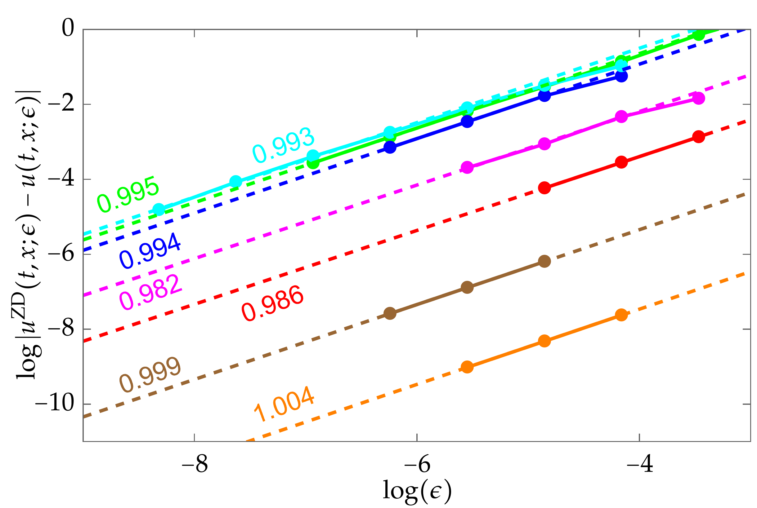
(29) u​(t,x;ϵ)=uZD​(t,x;ϵ)+𝒪​(ϵ)𝑢𝑡𝑥italic-ϵsuperscript𝑢ZD𝑡𝑥italic-ϵ𝒪italic-ϵu(t,x;\epsilon)=u^{\mathrm{ZD}}(t,x;\epsilon)+\mathcal{O}({\epsilon})

where the convergence is pointwise for such (t,x)𝑡𝑥(t,x) and also uniform on compact subsets of ℝ2∖𝒟superscriptℝ2𝒟\mathbb{R}^{2}\setminus\mathcal{D}.

Corollary 1.6 (Convergence in L2superscript𝐿2L^{2}).

Let u0∈L2​(ℝ)subscript𝑢0superscript𝐿2ℝu_{0}\in L^{2}(\mathbb{R}) be a rational initial condition of the form (11). If t≥0𝑡0t\geq 0 is such that J​(t,x)≤1𝐽𝑡𝑥1J(t,x)\leq 1 for every generic x𝑥x where J​(t,x)𝐽𝑡𝑥J(t,x) is well-defined, then as ϵ→0→italic-ϵ0\epsilon\to 0,

(30) u​(t,⋄;ϵ)=uZD​(t,⋄;ϵ)+oL2​(1).𝑢𝑡⋄italic-ϵsuperscript𝑢ZD𝑡⋄italic-ϵsubscript𝑜superscript𝐿21u(t,\diamond;\epsilon)=u^{\mathrm{ZD}}(t,\diamond;\epsilon)+o_{L^{2}}(1).

Remark 1.7.

It is reasonable to expect that (30) holds even at times t≥0𝑡0t\geq 0 for which J​(t,x)𝐽𝑡𝑥J(t,x) has any finite upper bound. However, the proof of Corollary 1.6 involves an averaging argument (see Lemma 7.3 below) that would need to be upgraded to a multiphase averaging argument if J​(t,x)≥2𝐽𝑡𝑥2J(t,x)\geq 2. Because such arguments are difficult to explain (Diophantine resonance conditions must be dealt with carefully), to keep the paper as simple as possible we leave the details to future work.

Remark 1.8.

Note that the zero-dispersion profile uZD​(t,x;ϵ)superscript𝑢ZD𝑡𝑥italic-ϵu^{\mathrm{ZD}}(t,x;\epsilon) still makes sense for non-rational initial data, however, the proof of Theorem 1.5 is open without the rational assumption. Indeed, using a rational approximation of the initial data is not sufficient, because known well-posedness results in the literature (see, for instance [26]) do not provide estimates on the modulus of continuity of the data-to-solution map that are uniform in the limit ϵ↓0↓italic-ϵ0\epsilon\downarrow 0. One may also notice that the approximation formula itself is very sensitive to small errors. For instance, looking at the simpler J​(t,x)=1𝐽𝑡𝑥1J(t,x)=1 version of the formula given in (26), one can see that even if the modulation variables ujB​(t,x)superscriptsubscript𝑢𝑗B𝑡𝑥u_{j}^{\mathrm{B}}(t,x), j=0,1,2𝑗012j=0,1,2, θ1​(t,x)subscript𝜃1𝑡𝑥\theta_{1}(t,x), and φ1​(t,x)subscript𝜑1𝑡𝑥\varphi_{1}(t,x) are perturbed by terms of size proportional to ϵitalic-ϵ\epsilon, one can still obtain errors not decaying to zero as ϵ→0→italic-ϵ0\epsilon\to 0 because of the factor ϵ−1superscriptitalic-ϵ1\epsilon^{-1} in the phase. This shows that, for example, a spatial translation of u0​(⋄)subscript𝑢0⋄u_{0}(\diamond) by a shift of order O​(ϵ)𝑂italic-ϵO(\epsilon) (which is an O​(ϵ1/2)𝑂superscriptitalic-ϵ12O(\epsilon^{1/2}) perturbation in L2​(ℝ)superscript𝐿2ℝL^{2}(\mathbb{R})) will lead to a leading-order phase shift in the approximation that will ruin the accuracy of the approximation.

1.4 Plan of the paper

We first recall from [6] the representation of the exact solution of the Cauchy initial-value problem for the Benjamin-Ono equation (3) with rational initial data of the form (11) in Section 2. Then, in Section 3, we explain the general idea of proof in the case of one pole N=1𝑁1N=1, so that J=0𝐽0J=0 or J=1𝐽1J=1.

In general, the analysis of the solution formula in the small-dispersion limit amounts to the (classical) steepest-descent analysis of a family of contour integrals, and for this approach to be effective it is first necessary to specify suitable contours of integration. In Section 4, we explain how to analyze the exponent function appearing in contour integrals in the solution formula by introducing the notion of extended level curves. Using this analysis, the specification of contours of integration is given in Section 5. The reader willing to accept the result stated at the beginning of Section 5 (Proposition 5.1) on first reading can skip ahead to Section 6, wherein the steepest descent method is applied and the resulting asymptotic formula is simplified, proving Theorem 1.5. We finally deduce Corollary 1.6 from Theorem 1.5 in Section 7. Section 8 is a short demonstration of the validity of Theorem 1.5 via numerics.

Acknowledgements

E. Blackstone was partially supported by the National Science Foundation under grant DMS-1812625. L. Gassot was supported by the France 2030 framework program, the Centre Henri Lebesgue ANR-11-LABX-0020-01, and the ANR project HEAD–ANR-24-CE40-3260. P. Gérard was partially supported by the French Agence Nationale de la Recherche under the ANR project ISAAC–ANR-23–CE40-0015-01. P. D. Miller was partially supported by the National Science Foundation under grant DMS-2204896. The authors would like to thank Matthew Mitchell for useful discussions.

2 The solution of Benjamin-Ono with rational initial data

Here we recall the result of [6], in which a general solution formula for the Cauchy problem of the Benjamin-Ono equation (3) with initial data in L2​(ℝ)superscript𝐿2ℝL^{2}(\mathbb{R}) was applied to rational initial data of the form (11).

We start with the real-valued Lax-Oleinik objective function h​(y)ℎ𝑦h(y) defined for y∈ℝ𝑦ℝy\in\mathbb{R} by (15). It will be necessary to analytically continue y↦h​(y)maps-to𝑦ℎ𝑦y\mapsto h(y) to a maximal domain that is generally more complicated than implied by using the principal branch of the logarithm in (15) and taking y=z𝑦𝑧y=z to be complex. To this end, we consider branch cuts {Γn,Γ¯n}n=1NsuperscriptsubscriptsubscriptΓ𝑛subscript¯Γ𝑛𝑛1𝑁\{\Gamma_{n},\bar{\Gamma}_{n}\}_{n=1}^{N} with the following properties.

Definition 2.1 (Branch cuts of hℎh).

The branch cuts Γ1,…,ΓNsubscriptΓ1…subscriptΓ𝑁\Gamma_{1},\dots,\Gamma_{N} are pairwise disjoint piecewise-smooth curves each emanating from exactly one of the poles {pn}n=1Nsuperscriptsubscriptsubscript𝑝𝑛𝑛1𝑁\{p_{n}\}_{n=1}^{N} and tending to z=∞𝑧z=\infty in the other direction asymptotic to the ray arg⁡(z)=3​π/4𝑧3𝜋4\arg(z)=3\pi/4, all of which lie in a half-plane Im​(z)>−δIm𝑧𝛿\mathrm{Im}(z)>-\delta for some δ>0𝛿0\delta>0 sufficiently small (in particular, we assume δ<minn⁡{Im​(pn)}𝛿subscript𝑛Imsubscript𝑝𝑛\delta<\min_{n}\{\mathrm{Im}(p_{n})\}. The branch cuts Γ¯1,…,Γ¯Nsubscript¯Γ1…subscript¯Γ𝑁\bar{\Gamma}_{1},\dots,\bar{\Gamma}_{N} are straight horizontal rays each emanating from exactly one of the conjugate poles {pn∗}n=1Nsuperscriptsubscriptsuperscriptsubscript𝑝𝑛𝑛1𝑁\{p_{n}^{*}\}_{n=1}^{N} and extending to z=∞𝑧z=\infty in the left half-plane.

Given the branch cuts, we index the poles {pn}n=1Nsuperscriptsubscriptsubscript𝑝𝑛𝑛1𝑁\{p_{n}\}_{n=1}^{N} such that in the vicinity of z=∞𝑧z=\infty in the upper half-plane, the branch cuts Γ1,…,ΓNsubscriptΓ1…subscriptΓ𝑁\Gamma_{1},\dots,\Gamma_{N} are ordered left-to-right. See Figure 3, left panel. We hence obtain a well-defined function z↦h​(z)maps-to𝑧ℎ𝑧z\mapsto h(z) by analytic continuation from large negative real values of z𝑧z where h​(z)ℎ𝑧h(z) is given by (15) to the domain z∈ℂ∖(Γ1∪⋯∪ΓN∪Γ¯1∪⋯∪Γ¯N)𝑧ℂsubscriptΓ1⋯subscriptΓ𝑁subscript¯Γ1⋯subscript¯Γ𝑁z\in\mathbb{C}\setminus(\Gamma_{1}\cup\cdots\cup\Gamma_{N}\cup\bar{\Gamma}_{1}\cup\cdots\cup\bar{\Gamma}_{N}).

We next define some relevant integration contours in the z𝑧z-plane. In the terminology of [6], the assumption that the rational initial condition is non-special (see Definition 4.7) means that all indices n=1,…,N𝑛1…𝑁n=1,\dots,N are non-exceptional, so we can provide a simplified definition.

Definition 2.2.

For n=1,…,N𝑛1…𝑁n=1,\dots,N, Cnsubscript𝐶𝑛C_{n} denotes a contour originating and terminating at z=∞𝑧z=\infty in the direction arg⁡(z)=3​π/4𝑧3𝜋4\arg(z)={3\pi/4}, lying in the domain of analyticity of h​(z)ℎ𝑧h(z), and encircling with counterclockwise orientation precisely the branch cuts of h​(z)ℎ𝑧h(z) emanating from each of the points z=pm𝑧subscript𝑝𝑚z=p_{m}, 1≤m≤n1𝑚𝑛1\leq m\leq n. In the special case that cn∈i​ϵ​ℕsubscript𝑐𝑛iitalic-ϵℕc_{n}\in\mathrm{i}\epsilon\mathbb{N}, Cnsubscript𝐶𝑛C_{n} terminates instead at z=pn𝑧subscript𝑝𝑛z=p_{n}. C0subscript𝐶0C_{0} denotes a path in the domain of analyticity of h​(z)ℎ𝑧h(z) originating at z=∞𝑧z=\infty in the direction arg⁡(z)=3​π/4𝑧3𝜋4\arg(z)={3\pi/4} to the left of all branch cuts Γ1,…,ΓNsubscriptΓ1…subscriptΓ𝑁\Gamma_{1},\dots,\Gamma_{N} of h​(z)ℎ𝑧h(z) and terminating at z=∞𝑧z=\infty in the direction arg⁡(z)=−π/4𝑧𝜋4\arg(z)=-{\pi/4}.

See the right-hand panel of Figure 3.

p1subscript𝑝1p_{1}p2subscript𝑝2p_{2}p3subscript𝑝3p_{3}p4subscript𝑝4p_{4}p5subscript𝑝5p_{5}p1∗superscriptsubscript𝑝1p_{1}^{*}p2∗superscriptsubscript𝑝2p_{2}^{*}p3∗superscriptsubscript𝑝3p_{3}^{*}p4∗superscriptsubscript𝑝4p_{4}^{*}p5∗superscriptsubscript𝑝5p_{5}^{*}Γ1subscriptΓ1\Gamma_{1}Γ2subscriptΓ2\Gamma_{2}Γ3subscriptΓ3\Gamma_{3}Γ4subscriptΓ4\Gamma_{4}Γ5subscriptΓ5\Gamma_{5}Γ¯1subscript¯Γ1\bar{\Gamma}_{1}Γ¯2subscript¯Γ2\bar{\Gamma}_{2}Γ¯3subscript¯Γ3\bar{\Gamma}_{3}Γ¯5subscript¯Γ5\bar{\Gamma}_{5}Γ¯4subscript¯Γ4\bar{\Gamma}_{4}δ𝛿\delta
C1subscript𝐶1C_{1}C2subscript𝐶2C_{2}C3subscript𝐶3C_{3}C4subscript𝐶4C_{4}C5subscript𝐶5C_{5}C0subscript𝐶0C_{0}
Figure 3: Left: admissible branch cuts of h​(z)ℎ𝑧h(z) in the z𝑧z-plane for a rational initial condition with N=5𝑁5N=5. Right: corresponding contours C1,C2,C3,C4,C5subscript𝐶1subscript𝐶2subscript𝐶3subscript𝐶4subscript𝐶5C_{1},C_{2},C_{3},C_{4},C_{5} and C0subscript𝐶0C_{0} in the general case that cn∉i​ϵ​ℕsubscript𝑐𝑛iitalic-ϵℕc_{n}\not\in\mathrm{i}\epsilon\mathbb{N} for each n𝑛n.

Given ϵ>0italic-ϵ0\epsilon>0 and t>0𝑡0t>0, we next define (N+1)×(N+1)𝑁1𝑁1(N+1)\times(N+1) matrices 𝐀​(t,x;ϵ)𝐀𝑡𝑥italic-ϵ\mathbf{A}(t,x;\epsilon) and 𝐁​(t,x;ϵ)𝐁𝑡𝑥italic-ϵ\mathbf{B}(t,x;\epsilon) as follows. For 1≤j≤N+11𝑗𝑁11\leq j\leq N+1 and 2≤k≤N+12𝑘𝑁12\leq k\leq N+1, set

(31) Aj​1​(t,x;ϵ):=∫Cj−1u0​(z)​e−i​h​(z)/ϵ​dz,assignsubscript𝐴𝑗1𝑡𝑥italic-ϵsubscriptsubscript𝐶𝑗1subscript𝑢0𝑧superscripteiℎ𝑧italic-ϵdifferential-d𝑧\displaystyle A_{j1}(t,x;\epsilon):=\int_{C_{j-1}}u_{0}(z)\mathrm{e}^{-\mathrm{i}h(z)/\epsilon}\,\mathrm{d}z, Aj​k​(t,x;ϵ):=∫Cj−1e−i​h​(z)/ϵ​d​zz−pk−1,assignsubscript𝐴𝑗𝑘𝑡𝑥italic-ϵsubscriptsubscript𝐶𝑗1superscripteiℎ𝑧italic-ϵd𝑧𝑧subscript𝑝𝑘1\displaystyle\quad A_{jk}(t,x;\epsilon):=\int_{C_{j-1}}\frac{\mathrm{e}^{-\mathrm{i}h(z)/\epsilon}\,\mathrm{d}z}{z-p_{k-1}},
(32) Bj​1​(t,x;ϵ):=∫Cj−1e−i​h​(z)/ϵ​dz,assignsubscript𝐵𝑗1𝑡𝑥italic-ϵsubscriptsubscript𝐶𝑗1superscripteiℎ𝑧italic-ϵdifferential-d𝑧\displaystyle B_{j1}(t,x;\epsilon):=\int_{C_{j-1}}\mathrm{e}^{-\mathrm{i}h(z)/\epsilon}\,\mathrm{d}z, Bj​k​(t,x;ϵ):=∫Cj−1e−i​h​(z)/ϵ​d​zz−pk−1=Aj​k​(t,x;ϵ).assignsubscript𝐵𝑗𝑘𝑡𝑥italic-ϵsubscriptsubscript𝐶𝑗1superscripteiℎ𝑧italic-ϵd𝑧𝑧subscript𝑝𝑘1subscript𝐴𝑗𝑘𝑡𝑥italic-ϵ\displaystyle\quad B_{jk}(t,x;\epsilon):=\int_{C_{j-1}}\frac{\mathrm{e}^{-\mathrm{i}h(z)/\epsilon}\,\mathrm{d}z}{z-p_{k-1}}=A_{jk}(t,x;\epsilon).

Then the main result of [6] is

Theorem 2.3 (Solution of Benjamin-Ono for rational initial data).

For each ϵ>0italic-ϵ0\epsilon>0, the exact solution of the Cauchy initial-value problem for the Benjamin-Ono equation (3) with rational initial condition u​(x,0;ϵ)=u0​(x)𝑢𝑥0italic-ϵsubscript𝑢0𝑥u(x,0;\epsilon)=u_{0}(x) of the form (11) is

(33) u​(t,x;ϵ)=2​R​e​(det(𝐀​(t,x;ϵ))det(𝐁​(t,x;ϵ))),t>0.formulae-sequence𝑢𝑡𝑥italic-ϵ2Re𝐀𝑡𝑥italic-ϵ𝐁𝑡𝑥italic-ϵ𝑡0u(t,x;\epsilon)=2\mathrm{Re}\left(\frac{\det(\mathbf{A}(t,x;\epsilon))}{\det(\mathbf{B}(t,x;\epsilon))}\right),\quad t>0.

Note that as shown in [6] the denominator cannot vanish for any (t,x)𝑡𝑥(t,x) with t>0𝑡0t>0, and that the formula returns the same result regardless of how the branch cuts and contours are chosen as long as they are consistent with Definitions 2.1 and 2.2 respectively.

Remark 2.4 (Change of contours).

The contours W1=C1subscript𝑊1subscript𝐶1W_{1}=C_{1}, W2=C2−C1subscript𝑊2subscript𝐶2subscript𝐶1W_{2}=C_{2}-C_{1}, W3=C3−C2subscript𝑊3subscript𝐶3subscript𝐶2W_{3}=C_{3}-C_{2},…, WN=CN−CN−1subscript𝑊𝑁subscript𝐶𝑁subscript𝐶𝑁1W_{N}=C_{N}-C_{N-1} (the notation meaning concatenation of the contours reversing orientation of the second one) each enclose just one of the branch cuts of hℎh. Conversely, given contours Wnsubscript𝑊𝑛W_{n}, n=1,…,N𝑛1…𝑁n=1,\dots,N, with Wnsubscript𝑊𝑛W_{n} enclosing only the branch cut of hℎh emanating from z=pn𝑧subscript𝑝𝑛z=p_{n} once in the counterclockwise sense (terminating at z=pn𝑧subscript𝑝𝑛z=p_{n} in the exceptional case that cn∈i​ϵ​ℕsubscript𝑐𝑛iitalic-ϵℕc_{n}\in\mathrm{i}\epsilon\mathbb{N}), we can take Cn=W1+W2+⋯+Wnsubscript𝐶𝑛subscript𝑊1subscript𝑊2⋯subscript𝑊𝑛C_{n}=W_{1}+W_{2}+\cdots+W_{n} (concatenation) as the contours in Definition 2.2. We make the identification W0=C0subscript𝑊0subscript𝐶0W_{0}=C_{0}. Since replacing the contours {Cn}n=0Nsuperscriptsubscriptsubscript𝐶𝑛𝑛0𝑁\{C_{n}\}_{n=0}^{N} in (31)–(32) with {Wn}n=0Nsuperscriptsubscriptsubscript𝑊𝑛𝑛0𝑁\{W_{n}\}_{n=0}^{N} amounts to multiplication of the matrices 𝐀​(t,x;ϵ)𝐀𝑡𝑥italic-ϵ\mathbf{A}(t,x;\epsilon) and 𝐁​(t,x;ϵ)𝐁𝑡𝑥italic-ϵ\mathbf{B}(t,x;\epsilon) on the left by the same invertible matrix (which happens to have unit determinant), the solution formula (33) in Theorem 2.3 is unchanged if we use {Wn}n=0Nsuperscriptsubscriptsubscript𝑊𝑛𝑛0𝑁\{W_{n}\}_{n=0}^{N} instead of {Cn}n=0Nsuperscriptsubscriptsubscript𝐶𝑛𝑛0𝑁\{C_{n}\}_{n=0}^{N} to define the integrals, and assuming non-special initial data u0subscript𝑢0u_{0}, we will do so going forward.

Remark 2.5 (Choice of new contours).

By the generalized Cauchy integral theorem, each contour Wnsubscript𝑊𝑛W_{n} can be taken to lie exactly along opposite sides of the branch cut ΓnsubscriptΓ𝑛\Gamma_{n} (along one side in the exceptional case that cn∈i​ϵ​ℕsubscript𝑐𝑛iitalic-ϵℕc_{n}\in\mathrm{i}\epsilon\mathbb{N}) except possibly near the pole pnsubscript𝑝𝑛p_{n}. Thus away from the pole pnsubscript𝑝𝑛p_{n}, the arcs on opposite sides of ΓnsubscriptΓ𝑛\Gamma_{n} may be taken to be exactly the same curves with opposite orientation and with the exponent h​(z)ℎ𝑧h(z) taking values differing by a constant. By a similar deformation argument, several pairwise disjoint branch cuts ΓnsubscriptΓ𝑛\Gamma_{n} “wrapped by” corresponding contours Wnsubscript𝑊𝑛W_{n} may be taken to lie in part against each other in the z𝑧z-plane.

3 The case of one pole

In this section, we give a general idea of proof of Theorem 1.5 in the case N=1𝑁1N=1 and p1=isubscript𝑝1ip_{1}=\mathrm{i}, assuming also for convenience that u0subscript𝑢0u_{0} and (t,x)𝑡𝑥(t,x) are in nonspecial configuration according to Definition 4.7 (see Section 4.3 below). Note that once we have chosen N=1𝑁1N=1, there is no loss of generality in assuming that p1=isubscript𝑝1ip_{1}=\mathrm{i} (by real translation and positive scaling in the complex z𝑧z-plane, compensating for the scaling by adding a real constant to h​(z)ℎ𝑧h(z)).

Let (t,x)∈ℝ2𝑡𝑥superscriptℝ2(t,x)\in\mathbb{R}^{2}. According to Theorem 2.3 and Remark 2.4, one can write

(34) u​(t,x;ϵ)=2​Re⁡(det(𝐀​(t,x;ϵ))det(𝐁​(t,x;ϵ))),𝑢𝑡𝑥italic-ϵ2Re𝐀𝑡𝑥italic-ϵ𝐁𝑡𝑥italic-ϵu(t,x;\epsilon)=2\operatorname{Re}\left(\frac{\det(\mathbf{A}(t,x;\epsilon))}{\det(\mathbf{B}(t,x;\epsilon))}\right),

where

(35) 𝐀​(t,x;ϵ)=[∫W0e−i​h​(z)/ϵ​u0​(z)​dz∫W0e−i​h​(z)/ϵ​d​zz−p1∫W1e−i​h​(z)/ϵ​u0​(z)​dz∫W1e−i​h​(z)/ϵ​d​zz−p1],𝐁​(t,x;ϵ)=[∫W0e−i​h​(z)/ϵ​dz∫W0e−i​h​(z)/ϵ​d​zz−p1∫W1e−i​h​(z)/ϵ​dz∫W1e−i​h​(z)/ϵ​d​zz−p1].formulae-sequence𝐀𝑡𝑥italic-ϵmatrixsubscriptsubscript𝑊0superscripteiℎ𝑧italic-ϵsubscript𝑢0𝑧differential-d𝑧subscriptsubscript𝑊0superscripteiℎ𝑧italic-ϵd𝑧𝑧subscript𝑝1subscriptsubscript𝑊1superscripteiℎ𝑧italic-ϵsubscript𝑢0𝑧differential-d𝑧subscriptsubscript𝑊1superscripteiℎ𝑧italic-ϵd𝑧𝑧subscript𝑝1𝐁𝑡𝑥italic-ϵmatrixsubscriptsubscript𝑊0superscripteiℎ𝑧italic-ϵdifferential-d𝑧subscriptsubscript𝑊0superscripteiℎ𝑧italic-ϵd𝑧𝑧subscript𝑝1subscriptsubscript𝑊1superscripteiℎ𝑧italic-ϵdifferential-d𝑧subscriptsubscript𝑊1superscripteiℎ𝑧italic-ϵd𝑧𝑧subscript𝑝1\begin{split}\mathbf{A}(t,x;\epsilon)&=\begin{bmatrix}\displaystyle\int_{W_{0}}\mathrm{e}^{-\mathrm{i}h(z)/\epsilon}u_{0}(z)\mathrm{d}z&\displaystyle\int_{W_{0}}\mathrm{e}^{-\mathrm{i}h(z)/\epsilon}\frac{\mathrm{d}z}{z-p_{1}}\\ \displaystyle\int_{W_{1}}\mathrm{e}^{-\mathrm{i}h(z)/\epsilon}u_{0}(z)\mathrm{d}z&\displaystyle\int_{W_{1}}\mathrm{e}^{-\mathrm{i}h(z)/\epsilon}\frac{\mathrm{d}z}{z-p_{1}}\\ \end{bmatrix},\\ \mathbf{B}(t,x;\epsilon)&=\begin{bmatrix}\displaystyle\int_{W_{0}}\mathrm{e}^{-\mathrm{i}h(z)/\epsilon}\mathrm{d}z&\displaystyle\int_{W_{0}}\mathrm{e}^{-\mathrm{i}h(z)/\epsilon}\frac{\mathrm{d}z}{z-p_{1}}\\ \displaystyle\int_{W_{1}}\mathrm{e}^{-\mathrm{i}h(z)/\epsilon}\mathrm{d}z&\displaystyle\int_{W_{1}}\mathrm{e}^{-\mathrm{i}h(z)/\epsilon}\frac{\mathrm{d}z}{z-p_{1}}\\ \end{bmatrix}.\end{split}

We write 2​c1=a−i​b2subscript𝑐1𝑎i𝑏2c_{1}=a-\mathrm{i}b where (a,b)∈ℝ2∖{(0,0)}𝑎𝑏superscriptℝ200(a,b)\in\mathbb{R}^{2}\setminus\{(0,0)\}, so that

(36) u0​(x)=a​x+bx2+1.subscript𝑢0𝑥𝑎𝑥𝑏superscript𝑥21u_{0}(x)=\frac{ax+b}{x^{2}+1}.

Equation (12) has three roots y0,y1,y2∈ℂsubscript𝑦0subscript𝑦1subscript𝑦2ℂy_{0},y_{1},y_{2}\in\mathbb{C}:

(37) (y−x)​(y2+1)+2​t​(a​y+b)=(y−y0)​(y−y1)​(y−y2).𝑦𝑥superscript𝑦212𝑡𝑎𝑦𝑏𝑦subscript𝑦0𝑦subscript𝑦1𝑦subscript𝑦2(y-x)(y^{2}+1)+2t(ay+b)=(y-y_{0})(y-y_{1})(y-y_{2}).

When J=0𝐽0J=0, then y0subscript𝑦0y_{0} is real and the other two are a complex-conjugate pair denoted y1=z1∈ℂ+subscript𝑦1subscript𝑧1subscriptℂy_{1}=z_{1}\in\mathbb{C}_{+} and y2=z1∗subscript𝑦2superscriptsubscript𝑧1y_{2}=z_{1}^{*}, and when J=1𝐽1J=1, the roots y0>y1>y2subscript𝑦0subscript𝑦1subscript𝑦2y_{0}>y_{1}>y_{2} are all real.

3.1 Determination of suitable branch cuts and integration contours

The first step is to carefully choose the branch cut of h​(z)=h​(z;t,x)ℎ𝑧ℎ𝑧𝑡𝑥h(z)=h(z;t,x), denoted Γ1subscriptΓ1\Gamma_{1}. Then, we choose the contours W0subscript𝑊0W_{0}, W1subscript𝑊1W_{1} in ℂ∖Γ1ℂsubscriptΓ1\mathbb{C}\setminus\Gamma_{1} consistent with Definition 2.2 and Remark 2.4 such that the integrals along each contour are dominated by contributions from different critical points of h​(z)ℎ𝑧h(z) so that the leading term of the determinants of 𝐀​(t,x;ϵ)𝐀𝑡𝑥italic-ϵ\mathbf{A}(t,x;\epsilon) and 𝐁​(t,x;ϵ)𝐁𝑡𝑥italic-ϵ\mathbf{B}(t,x;\epsilon) can be computed as the determinants of the leading terms of the matrix elements themselves. We claim that the following proposition is true (see Proposition 5.1 for the general case with proof).

Proposition 3.1 (Existence of steepest descent contours when N=1𝑁1N=1).

There exist contours W0,W1subscript𝑊0subscript𝑊1W_{0},W_{1} related to contours of Definition 2.2 according to Remark 2.4 and such that one of the following alternatives hold.

If J=0𝐽0J=0,

  • •

    on the contour W0subscript𝑊0W_{0}, Re⁡(−i​h​(z))Reiℎ𝑧\operatorname{Re}(-\mathrm{i}h(z)) achieves its maximal value only at y0∈ℝsubscript𝑦0ℝy_{0}\in\mathbb{R};

  • •

    on the contour W1subscript𝑊1W_{1}, Re⁡(−i​h​(z))Reiℎ𝑧\operatorname{Re}(-\mathrm{i}h(z)) achieves its maximal value only at z1∈ℂ+subscript𝑧1subscriptℂz_{1}\in\mathbb{C}_{+} and only on one side of the branch cut Γ1subscriptΓ1\Gamma_{1}.

If J=1𝐽1J=1,

  • •

    on the contour W0subscript𝑊0W_{0}, Re⁡(−i​h​(z))Reiℎ𝑧\operatorname{Re}(-\mathrm{i}h(z)) achieves its maximal value only at y0,y1subscript𝑦0subscript𝑦1y_{0},y_{1} and y2subscript𝑦2y_{2};

  • •

    on the contour W1subscript𝑊1W_{1}, Re⁡(−i​h​(z))Reiℎ𝑧\operatorname{Re}(-\mathrm{i}h(z)) achieves its maximal value only at y1,y2subscript𝑦1subscript𝑦2y_{1},y_{2} and only on one side of the branch cut Γ1subscriptΓ1\Gamma_{1}.

p1subscript𝑝1p_{1}y2subscript𝑦2y_{2}y1subscript𝑦1y_{1}y0subscript𝑦0y_{0}W0subscript𝑊0W_{0}W1subscript𝑊1W_{1}y0,βsubscript𝑦0𝛽y_{0,\beta}y0,αsubscript𝑦0𝛼y_{0,\alpha}
Figure 4: The union of the red curves is the branch cut Γ1subscriptΓ1\Gamma_{1}, emanating from the pole p1subscript𝑝1p_{1} in a J​(t,x)=1𝐽𝑡𝑥1J(t,x)=1 scenario. The black curves are the critical trajectories Re​(−i​h​(z))=0Reiℎ𝑧0\mathrm{Re}(-\mathrm{i}h(z))=0 oriented according to increasing parametrization by s𝑠s, and the blue curves W0subscript𝑊0W_{0}, W1subscript𝑊1W_{1} are the integration contours. The dashed blue line segments passing y2subscript𝑦2y_{2}, y1subscript𝑦1y_{1}, y0subscript𝑦0y_{0} are to be understood as local steepest descent contours passing through their respective saddle points.

The idea of the proof of this Proposition (and its generalization in Section 5) is to construct a systematic method (for each (t,x)𝑡𝑥(t,x)) of selecting various extended level curves to create the branch cut Γ1subscriptΓ1\Gamma_{1} emanating from the pole p1subscript𝑝1p_{1} with desirable properties. The steepest descent contour W1subscript𝑊1W_{1} then travels along each side of the branch cut Γ1subscriptΓ1\Gamma_{1} (with a small exception around p1subscript𝑝1p_{1}), see Remark 2.5. The remaining contour W0subscript𝑊0W_{0} has a slightly different construction but is also specified in a similar systematic way. See Figure 4 for an example of Γ1subscriptΓ1\Gamma_{1} and W0subscript𝑊0W_{0}, W1subscript𝑊1W_{1} in an N=J​(t,x)=1𝑁𝐽𝑡𝑥1N=J(t,x)=1 scenario. We note that dashed blue paths on top of Γ1subscriptΓ1\Gamma_{1} along the local steepest descent paths over y2subscript𝑦2y_{2}, y1subscript𝑦1y_{1} are traversed once on each side of Γ1subscriptΓ1\Gamma_{1} for W1subscript𝑊1W_{1} and that W1subscript𝑊1W_{1} (and Γ1subscriptΓ1\Gamma_{1}) tend to ∞\infty in the direction arg⁡(z)=3​π/4𝑧3𝜋4\arg(z)=3\pi/4. The contour W0subscript𝑊0W_{0} is the union of

  • •

    the lower side of W1subscript𝑊1W_{1} until reaching the point y0,αsubscript𝑦0𝛼y_{0,\alpha},

  • •

    the dashed blue local steepest descent contour over y0subscript𝑦0y_{0} which connects y0,αsubscript𝑦0𝛼y_{0,\alpha} to y0,βsubscript𝑦0𝛽y_{0,\beta},

  • •

    the blue path from y0,βsubscript𝑦0𝛽y_{0,\beta} that tends to ∞\infty in the direction arg⁡(z)=−π/4𝑧𝜋4\arg(z)=-\pi/4.

3.2 Steepest descent analysis

The second step, detailed in Section 6 below in the general case, relies on the steepest descent method applied to the integrals in (35). When N=1𝑁1N=1, we choose W0subscript𝑊0W_{0}, W1subscript𝑊1W_{1} as described in Proposition 3.1.

Lemma 3.2 (Steepest descent method).

Suppose u0subscript𝑢0u_{0} and (t,x)𝑡𝑥(t,x) are in non-special configuration (see Definition 4.7 below), and ϵ>0italic-ϵ0\epsilon>0 is sufficiently small. Then,

(38) ∫We−i​h​(z;t,x)/ϵ​F​(z)​dz=ei​φ​(t,x)​F​(ζ)​2​π​ϵ|h′′​(ζ;t,x)|​e−i​h​(ζ;t,x)/ϵ​(1+𝒪​(ϵ)),subscript𝑊superscripteiℎ𝑧𝑡𝑥italic-ϵ𝐹𝑧differential-d𝑧superscriptei𝜑𝑡𝑥𝐹𝜁2𝜋italic-ϵsuperscriptℎ′′𝜁𝑡𝑥superscripteiℎ𝜁𝑡𝑥italic-ϵ1𝒪italic-ϵ\int_{W}\mathrm{e}^{-\mathrm{i}h(z;t,x)/\epsilon}F(z)\,\mathrm{d}z=\mathrm{e}^{\mathrm{i}\varphi(t,x)}F(\zeta)\sqrt{\frac{2\pi\epsilon}{|h^{\prime\prime}(\zeta;t,x)|}}\mathrm{e}^{-\mathrm{i}h(\zeta;t,x)/\epsilon}\left(1+\mathcal{O}(\epsilon)\right),

where F​(z)𝐹𝑧F(z) is analytic in a neighborhood of W𝑊W, a contour arc along which Im​(−i​h​(z;t,x))Imiℎ𝑧𝑡𝑥\mathrm{Im}(-\mathrm{i}h(z;t,x)) is constant and Re​(−i​h​(z;t,x))Reiℎ𝑧𝑡𝑥\mathrm{Re}(-\mathrm{i}h(z;t,x)) achieves its maximum value at z=ζ∈W𝑧𝜁𝑊z=\zeta\in W. The point z=ζ𝑧𝜁z=\zeta is a simple critical point of h​(z;t,x)ℎ𝑧𝑡𝑥h(z;t,x) at which the tangent to the contour W𝑊W makes an angle of φ​(t,x)𝜑𝑡𝑥\varphi(t,x) with the direction arg⁡(z−ζ)=0𝑧𝜁0\arg(z-\zeta)=0. Moreover, the error term is uniform for (t,x)𝑡𝑥(t,x) in any connected component of the same set where J​(t,x)𝐽𝑡𝑥J(t,x) remains constant.

The uniformity of the error term follows from the fact that u0subscript𝑢0u_{0} and (t,x)𝑡𝑥(t,x) being in non-special configuration guarantees that the critical points of h​(z;t,x)ℎ𝑧𝑡𝑥h(z;t,x) will be simple. Hence Lemma 3.2 also applies for calculating the matrix elements of 𝐀​(t,x;ϵ)𝐀𝑡𝑥italic-ϵ\mathbf{A}(t,x;\epsilon) and 𝐁​(t,x;ϵ)𝐁𝑡𝑥italic-ϵ\mathbf{B}(t,x;\epsilon) if only (t,x)∈ℝ2∖𝒟𝑡𝑥superscriptℝ2𝒟(t,x)\in\mathbb{R}^{2}\setminus\mathcal{D} as is required in Theorem 1.5.

Case J=0𝐽0J=0

Applying the above Lemma to (34) yields

(39) u​(t,x;ϵ)=2​Re⁡(det(𝐀0​(t,x))det(𝐁0​(t,x)))+𝒪​(ϵ),𝑢𝑡𝑥italic-ϵ2Resuperscript𝐀0𝑡𝑥superscript𝐁0𝑡𝑥𝒪italic-ϵu(t,x;\epsilon)=2\operatorname{Re}\left(\frac{\det(\mathbf{A}^{0}(t,x))}{\det(\mathbf{B}^{0}(t,x))}\right)+\mathcal{O}({\epsilon}),

where

(40) 𝐀0​(t,x)=[u0​(y0)1y0−p1u0​(y2)1y2−p1],𝐁0​(t,x)=[11y0−p111y2−p1].formulae-sequencesuperscript𝐀0𝑡𝑥matrixsubscript𝑢0subscript𝑦01subscript𝑦0subscript𝑝1subscript𝑢0subscript𝑦21subscript𝑦2subscript𝑝1superscript𝐁0𝑡𝑥matrix11subscript𝑦0subscript𝑝111subscript𝑦2subscript𝑝1\mathbf{A}^{0}(t,x)=\begin{bmatrix}u_{0}(y_{0})&\displaystyle\frac{1}{y_{0}-p_{1}}\\ u_{0}(y_{2})&\displaystyle\frac{1}{y_{2}-p_{1}}\\ \end{bmatrix},\quad\mathbf{B}^{0}(t,x)=\begin{bmatrix}1&\displaystyle\frac{1}{y_{0}-p_{1}}\\ 1&\displaystyle\frac{1}{y_{2}-p_{1}}\\ \end{bmatrix}.

According to (12), u0​(yj)=(x−yj)/(2​t)subscript𝑢0subscript𝑦𝑗𝑥subscript𝑦𝑗2𝑡u_{0}(y_{j})=(x-y_{j})/(2t), so evaluating the determinants in (39) gives

(41) u​(t,x;ϵ)=−1t​Re⁡(−x+y0+y2−p1)+𝒪​(ϵ).𝑢𝑡𝑥italic-ϵ1𝑡Re𝑥subscript𝑦0subscript𝑦2subscript𝑝1𝒪italic-ϵu(t,x;\epsilon)=-\frac{1}{t}\operatorname{Re}(-x+y_{0}+y_{2}-p_{1})+\mathcal{O}({\epsilon}).

In the special case p1=isubscript𝑝1ip_{1}=\mathrm{i}, then y0+y1+y2=xsubscript𝑦0subscript𝑦1subscript𝑦2𝑥y_{0}+y_{1}+y_{2}=x thanks to (37) and since (x−y0)/(2​t)=u0B𝑥subscript𝑦02𝑡subscriptsuperscript𝑢𝐵0(x-y_{0})/(2t)=u^{B}_{0}, we conclude that

(42) u​(t,x;ϵ)=u0B​(t,x)+𝒪​(ϵ).𝑢𝑡𝑥italic-ϵsubscriptsuperscript𝑢𝐵0𝑡𝑥𝒪italic-ϵu(t,x;\epsilon)=u^{B}_{0}(t,x)+\mathcal{O}({\epsilon}).
Case J=1𝐽1J=1

In this case, the steepest descent angle is ϕ=−π/4italic-ϕ𝜋4\phi=-\pi/4 at y0subscript𝑦0y_{0} and y2subscript𝑦2y_{2}, and ϕ=π/4italic-ϕ𝜋4\phi=\pi/4 at y1subscript𝑦1y_{1}. Applying Lemma 3.2, we remove the factor e−i​π/4−i​h​(y0)/ϵ/|h′′​(y0)|superscriptei𝜋4iℎsubscript𝑦0italic-ϵsuperscriptℎ′′subscript𝑦0\mathrm{e}^{-\mathrm{i}{\pi}/{4}-\mathrm{i}{h(y_{0})}/{\epsilon}}/\sqrt{|h^{\prime\prime}(y_{0})|} from the first row of both determinants in (34), and e−i​π/4−i​h​(y2)/ϵ/|h′′​(y2)|superscriptei𝜋4iℎsubscript𝑦2italic-ϵsuperscriptℎ′′subscript𝑦2\mathrm{e}^{-\mathrm{i}{\pi}/{4}-\mathrm{i}{h(y_{2})}/{\epsilon}}/\sqrt{|h^{\prime\prime}(y_{2})|} from the second row. To simplify the notation, we define

(43) α:=−i​|h′′​(y1)||h′′​(y2)|​ei​(h​(y1)−h​(y2))/ϵ.assign𝛼isuperscriptℎ′′subscript𝑦1superscriptℎ′′subscript𝑦2superscripteiℎsubscript𝑦1ℎsubscript𝑦2italic-ϵ\alpha:=-\mathrm{i}\frac{\sqrt{|h^{\prime\prime}(y_{1})|}}{\sqrt{|h^{\prime\prime}(y_{2})|}}\mathrm{e}^{\mathrm{i}{(h(y_{1})-h(y_{2}))}/{\epsilon}}.

Thus we obtain (39) with the understanding that now

(44) 𝐀0​(t,x;ϵ)=[u0​(y2)+α​u0​(y1)1y2−p1+αy1−p1u0​(y0)1y0−p1],𝐁0​(t,x;ϵ)=[1+α1y2−p1+αy1−p111y0−p1].formulae-sequencesuperscript𝐀0𝑡𝑥italic-ϵmatrixsubscript𝑢0subscript𝑦2𝛼subscript𝑢0subscript𝑦11subscript𝑦2subscript𝑝1𝛼subscript𝑦1subscript𝑝1subscript𝑢0subscript𝑦01subscript𝑦0subscript𝑝1superscript𝐁0𝑡𝑥italic-ϵmatrix1𝛼1subscript𝑦2subscript𝑝1𝛼subscript𝑦1subscript𝑝111subscript𝑦0subscript𝑝1\begin{split}\mathbf{A}^{0}(t,x;\epsilon)&=\begin{bmatrix}u_{0}(y_{2})+\alpha u_{0}(y_{1})&\displaystyle{\frac{1}{y_{2}-p_{1}}+\frac{\alpha}{y_{1}-p_{1}}}\\ u_{0}(y_{0})&\displaystyle{\frac{1}{y_{0}-p_{1}}}\end{bmatrix},\\ \mathbf{B}^{0}(t,x;\epsilon)&=\begin{bmatrix}1+\alpha&\displaystyle{\frac{1}{y_{2}-p_{1}}+\frac{\alpha}{y_{1}-p_{1}}}\\ 1&\displaystyle{\frac{1}{y_{0}-p_{1}}}\end{bmatrix}.\end{split}

Using that u0​(yj)=(x−yj)/(2​t)subscript𝑢0subscript𝑦𝑗𝑥subscript𝑦𝑗2𝑡u_{0}(y_{j})=(x-y_{j})/(2t), we have the simplicification

(45) 𝐀0​(t,x;ϵ)=12​t​[x−y1+α​(x−y2)1y1−p1+αy2−p1x−y01y0−p1].superscript𝐀0𝑡𝑥italic-ϵ12𝑡matrix𝑥subscript𝑦1𝛼𝑥subscript𝑦21subscript𝑦1subscript𝑝1𝛼subscript𝑦2subscript𝑝1𝑥subscript𝑦01subscript𝑦0subscript𝑝1\mathbf{A}^{0}(t,x;\epsilon)=\frac{1}{2t}\begin{bmatrix}x-y_{1}+\alpha(x-y_{2})&\displaystyle{\frac{1}{y_{1}-p_{1}}+\frac{\alpha}{y_{2}-p_{1}}}\\ x-y_{0}&\displaystyle{\frac{1}{y_{0}-p_{1}}}\end{bmatrix}.

We adopt the notation of [23, Lemma 8] and denote

(46) A​(y):=|y1y−p1y01y0−p1|,B​(y):=|11y−p111y0−p1|.formulae-sequenceassign𝐴𝑦matrix𝑦1𝑦subscript𝑝1subscript𝑦01subscript𝑦0subscript𝑝1assign𝐵𝑦matrix11𝑦subscript𝑝111subscript𝑦0subscript𝑝1A(y):=\begin{vmatrix}y&\displaystyle{\frac{1}{y-p_{1}}}\\ y_{0}&\displaystyle{\frac{1}{y_{0}-p_{1}}}\end{vmatrix},\quad B(y):=\begin{vmatrix}1&\displaystyle{\frac{1}{y-p_{1}}}\\ 1&\displaystyle{\frac{1}{y_{0}-p_{1}}}\end{vmatrix}.

By linearity, we can expand both determinants along the first row, so that

(47) u​(t,x;ϵ)=1t​Re⁡(x​(B​(y1)+α​B​(y2))−(A​(y1)+α​A​(y2))B​(y1)+α​B​(y2))+𝒪​(ϵ).𝑢𝑡𝑥italic-ϵ1𝑡Re𝑥𝐵subscript𝑦1𝛼𝐵subscript𝑦2𝐴subscript𝑦1𝛼𝐴subscript𝑦2𝐵subscript𝑦1𝛼𝐵subscript𝑦2𝒪italic-ϵu(t,x;\epsilon)=\frac{1}{t}\operatorname{Re}\left(\frac{x\left(B(y_{1})+\alpha B(y_{2})\right)-\left(A(y_{1})+\alpha A(y_{2})\right)}{B(y_{1})+\alpha B(y_{2})}\right)+\mathcal{O}(\epsilon).

According to [23, Lemma 8], or via a direct calculation, we have that

(48) A​(y)=(y+y0−p1)​B​(y).𝐴𝑦𝑦subscript𝑦0subscript𝑝1𝐵𝑦A(y)=\left(y+y_{0}-p_{1}\right)B(y).

Consequently,

(49) u​(t,x;ϵ)=1t​Re⁡(x−y0+p1−y1​B​(y1)+α​y2​B​(y2)B​(y1)+α​B​(y2))+𝒪​(ϵ).𝑢𝑡𝑥italic-ϵ1𝑡Re𝑥subscript𝑦0subscript𝑝1subscript𝑦1𝐵subscript𝑦1𝛼subscript𝑦2𝐵subscript𝑦2𝐵subscript𝑦1𝛼𝐵subscript𝑦2𝒪italic-ϵu(t,x;\epsilon)=\frac{1}{t}\operatorname{Re}\left(x-y_{0}+p_{1}-\frac{y_{1}B(y_{1})+\alpha y_{2}B(y_{2})}{B(y_{1})+\alpha B(y_{2})}\right)+\mathcal{O}(\epsilon).

Taking the real part, since we assumed that p1=isubscript𝑝1ip_{1}=\mathrm{i}, we have

(50) u​(t,x;ϵ)=u0B−(u2B−u1B)​(|B​(y1)|2−|α|2​|B​(y2)|2)|B​(y1)|2+|α|2​|B​(y2)|2+α​B​(y2)​B​(y1)¯+α¯​B​(y2)¯​B​(y1)+𝒪​(ϵ).𝑢𝑡𝑥italic-ϵsubscriptsuperscript𝑢𝐵0subscriptsuperscript𝑢𝐵2subscriptsuperscript𝑢𝐵1superscript𝐵subscript𝑦12superscript𝛼2superscript𝐵subscript𝑦22superscript𝐵subscript𝑦12superscript𝛼2superscript𝐵subscript𝑦22𝛼𝐵subscript𝑦2¯𝐵subscript𝑦1¯𝛼¯𝐵subscript𝑦2𝐵subscript𝑦1𝒪italic-ϵu(t,x;\epsilon)=u^{B}_{0}-\frac{(u^{B}_{2}-u^{B}_{1})\left(|B(y_{1})|^{2}-|\alpha|^{2}|B(y_{2})|^{2}\right)}{|B(y_{1})|^{2}+|\alpha|^{2}|B(y_{2})|^{2}+\alpha B(y_{2})\overline{B(y_{1})}+\overline{\alpha}\overline{B(y_{2})}B(y_{1})}+\mathcal{O}(\epsilon).

Taking the derivative of equality (16) at y2subscript𝑦2y_{2} and y1subscript𝑦1y_{1}, we know for p1=isubscript𝑝1ip_{1}=\mathrm{i} that

(51) |α|2=|h′′​(y1)||h′′​(y2)|=y0−y1y0−y2⋅y22+1y12+1,superscript𝛼2superscriptℎ′′subscript𝑦1superscriptℎ′′subscript𝑦2⋅subscript𝑦0subscript𝑦1subscript𝑦0subscript𝑦2superscriptsubscript𝑦221superscriptsubscript𝑦121|\alpha|^{2}=\frac{|h^{\prime\prime}(y_{1})|}{|h^{\prime\prime}(y_{2})|}=\frac{y_{0}-y_{1}}{y_{0}-y_{2}}\cdot\frac{y_{2}^{2}+1}{y_{1}^{2}+1},

and

(52) B​(y2)=y2−y0(y2−i)​(y0+i),B​(y1)=y1−y0(y1−i)​(y0+i).formulae-sequence𝐵subscript𝑦2subscript𝑦2subscript𝑦0subscript𝑦2isubscript𝑦0i𝐵subscript𝑦1subscript𝑦1subscript𝑦0subscript𝑦1isubscript𝑦0iB(y_{2})=\frac{y_{2}-y_{0}}{(y_{2}-\mathrm{i})(y_{0}+\mathrm{i})},\quad B(y_{1})=\frac{y_{1}-y_{0}}{(y_{1}-\mathrm{i})(y_{0}+\mathrm{i})}.

Consequently we simplify u𝑢u as

(53) u​(t,x;ϵ)=u0B−(u2B−u1B)​(y2−y1)(2​y0−y2−y1)−2​(y0−y2)​(y0−y1)​cos⁡(θ/ϵ+φ)+𝒪​(ϵ),𝑢𝑡𝑥italic-ϵsubscriptsuperscript𝑢𝐵0subscriptsuperscript𝑢𝐵2subscriptsuperscript𝑢𝐵1subscript𝑦2subscript𝑦12subscript𝑦0subscript𝑦2subscript𝑦12subscript𝑦0subscript𝑦2subscript𝑦0subscript𝑦1𝜃italic-ϵ𝜑𝒪italic-ϵu(t,x;\epsilon)=u^{B}_{0}-\frac{(u^{B}_{2}-u^{B}_{1})(y_{2}-y_{1})}{(2y_{0}-y_{2}-y_{1})-2\sqrt{(y_{0}-y_{2})(y_{0}-y_{1})}\cos(\theta/\epsilon+\varphi)}+\mathcal{O}(\epsilon),

where

(54) θ​(t,x)=h​(y1)−h​(y2),φ=arg⁡(y1−i)−arg⁡(y2−i)+π2.formulae-sequence𝜃𝑡𝑥ℎsubscript𝑦1ℎsubscript𝑦2𝜑subscript𝑦1isubscript𝑦2i𝜋2\theta(t,x)=h(y_{1})-h(y_{2}),\quad\varphi=\arg(y_{1}-\mathrm{i})-\arg(y_{2}-\mathrm{i})+\frac{\pi}{2}.

Knowing that (yj−x)/(2​t)=−u0​(yj)subscript𝑦𝑗𝑥2𝑡subscript𝑢0subscript𝑦𝑗(y_{j}-x)/(2t)=-u_{0}(y_{j}), and recalling the definition of r𝑟r in (27), one can also write

(55) u​(t,x;ϵ)=u0B​(t,x)+(u2B​(t,x)−u1B​(t,x))​(1−r​(t,x)2)1+r​(t,x)2−2​r​cos⁡(θ​(t,x)/ϵ+φ​(t,x))+𝒪​(ϵ),𝑢𝑡𝑥italic-ϵsubscriptsuperscript𝑢𝐵0𝑡𝑥subscriptsuperscript𝑢𝐵2𝑡𝑥subscriptsuperscript𝑢𝐵1𝑡𝑥1𝑟superscript𝑡𝑥21𝑟superscript𝑡𝑥22𝑟𝜃𝑡𝑥italic-ϵ𝜑𝑡𝑥𝒪italic-ϵu(t,x;\epsilon)=u^{B}_{0}(t,x)+\frac{(u^{B}_{2}(t,x)-u^{B}_{1}(t,x))(1-r(t,x)^{2})}{1+r(t,x)^{2}-2r\cos(\theta(t,x)/\epsilon+\varphi(t,x))}+\mathcal{O}(\epsilon),

which is in agreement with (26). The quantity φ​(t,x)𝜑𝑡𝑥\varphi(t,x) can then be further expressed in a form involving only the profile of u0subscript𝑢0u_{0} on the real line by using Lemma 6.18 below.

4 Extended level curves

The exponent in the contour integrals (31), (32) is the function E​(z)𝐸𝑧E(z) defined by

(56) E​(z):=−i​h​(z).assign𝐸𝑧iℎ𝑧E(z):=-\mathrm{i}h(z).

The function z↦Re​(E​(z))maps-to𝑧Re𝐸𝑧z\mapsto\mathrm{Re}(E(z)) is well-defined and harmonic away from certain branch cuts emanating from {pn,pn∗}n=1Nsuperscriptsubscriptsubscript𝑝𝑛superscriptsubscript𝑝𝑛𝑛1𝑁\{p_{n},p_{n}^{*}\}_{n=1}^{N} consistent with Definition 2.1. In this domain the level set {z∈ℂ:Re​(E​(z))=L}conditional-set𝑧ℂRe𝐸𝑧𝐿\{z\in\mathbb{C}:\mathrm{Re}(E(z))=L\} for a given L∈ℝ𝐿ℝL\in\mathbb{R} is a union of analytic arcs called level curves. A level curve is locally characterized by the zero-increment condition

(57) Re​(E′​(z)​d​z)=Im​(h′​(z)​d​z)=0.Resuperscript𝐸′𝑧d𝑧Imsuperscriptℎ′𝑧d𝑧0\mathrm{Re}(E^{\prime}(z)\,\mathrm{d}z)=\mathrm{Im}(h^{\prime}(z)\,\mathrm{d}z)=0.

Since z↦h′​(z)maps-to𝑧superscriptℎ′𝑧z\mapsto h^{\prime}(z) defined by (16) with (11) is a meromorphic function on the whole z𝑧z-plane, the zero-increment condition makes sense even on the branch cuts of z↦Re​(E​(z))maps-to𝑧Re𝐸𝑧z\mapsto\mathrm{Re}(E(z)) and allows the level curve to be analytically continued through any branch cut. We call an analytic arc satisfying at every point the zero-increment condition, whether or not it intersects a branch cut, an extended level curve. If an extended level curve crosses a branch cut transversely, then Re​(E​(z))Re𝐸𝑧\mathrm{Re}(E(z)) generally evaluates to two different constants on the arcs of the curve separated by the branch cut.

The main point is that the extended level curves are well-defined even without specifying any branch cuts of h​(z)ℎ𝑧h(z) at all, so we can use them to actually determine branch cuts that will be suitable for subsequent steepest-descent analysis of the contour integrals. The extended level curves have two different interpretations that will be useful to us:

  • •

    as trajectories of a quadratic differential;

  • •

    as integral curves of an analytic vector field.

4.1 Extended level curves as trajectories of a quadratic differential

In the field of geometric function theory, a quadratic differential on the Riemann sphere with parameter z∈ℂ∪{∞}𝑧ℂz\in\mathbb{C}\cup\{\infty\} is an expression of the form Q​(z)​d​z2𝑄𝑧dsuperscript𝑧2Q(z)\,\mathrm{d}z^{2} where Q​(z)𝑄𝑧Q(z) is a rational function. By a trajectory of the quadratic differential we mean a maximal arc s↦z​(s)maps-to𝑠𝑧𝑠s\mapsto z(s) along which Q​(z​(s))​z′​(s)2>0𝑄𝑧𝑠superscript𝑧′superscript𝑠20Q(z(s))z^{\prime}(s)^{2}>0, often abbreviated to Q​(z)​d​z2>0𝑄𝑧dsuperscript𝑧20Q(z)\,\mathrm{d}z^{2}>0. There are many results describing the trajectories locally near the poles and zeros of Q​(z)𝑄𝑧Q(z) as well as globally on the sphere. As general references, we recommend the books of Jenkins [24] and Strebel [33]. The zero-increment condition (57) fits into this framework if we define the rational function Q​(z)𝑄𝑧Q(z) as a perfect square: Q​(z):=h′​(z)2assign𝑄𝑧superscriptℎ′superscript𝑧2Q(z):=h^{\prime}(z)^{2}; thus the extended level curves are precisely the trajectories of the quadratic differential Q​(z)​d​z2=h′​(z)2​d​z2𝑄𝑧dsuperscript𝑧2superscriptℎ′superscript𝑧2dsuperscript𝑧2Q(z)\,\mathrm{d}z^{2}=h^{\prime}(z)^{2}\,\mathrm{d}z^{2}.

One can see by taking a square root that in general the trajectories of a quadratic differential are locally integral curves of a certain vector field; however since the sign of the square root is arbitrary there is no a priori orientation of these curves, and moreover if Q​(z)𝑄𝑧\sqrt{Q(z)} has branch points it is impossible to assign a global orientation to the trajectories. This can lead to some strange behavior not found in the theory of single-valued vector fields such as trajectories with topological closure having nonempty interior (so-called divergent or recurrent trajectories). On the other hand, since Q​(z)𝑄𝑧Q(z) is a rational function, trajectories of quadratic differentials also have some more regular behavior than typical vector fields guarantee. For instance, a trajectory of a quadratic differential cannot approach a limit cycle in the plane in either direction.

4.2 Extended level curves as integral curves of an analytic vector field

At each point z=u+i​v∈ℂ∖{pn,pn∗}n=1N𝑧𝑢i𝑣ℂsuperscriptsubscriptsubscript𝑝𝑛superscriptsubscript𝑝𝑛𝑛1𝑁z=u+\mathrm{i}v\in\mathbb{C}\setminus\{p_{n},p_{n}^{*}\}_{n=1}^{N} the zero-increment condition (57) is equivalent to the renormalized form

(58) Im​(f​(u,v)​h′​(u+i​v)​(d​u+id​v))=0,Im𝑓𝑢𝑣superscriptℎ′𝑢i𝑣d𝑢id𝑣0\mathrm{Im}(f(u,v)h^{\prime}(u+\mathrm{i}v)\,(\mathrm{d}u+\mathrm{i}\mathrm{d}v))=0,

where f​(u,v)≥0𝑓𝑢𝑣0f(u,v)\geq 0 is the function

(59) f​(u,v):=∏n=1N|u+i​v−pn|2​|u+i​v−pn∗|2.assign𝑓𝑢𝑣superscriptsubscriptproduct𝑛1𝑁superscript𝑢i𝑣subscript𝑝𝑛2superscript𝑢i𝑣superscriptsubscript𝑝𝑛2f(u,v):=\prod_{n=1}^{N}|u+\mathrm{i}v-p_{n}|^{2}|u+\mathrm{i}v-p_{n}^{*}|^{2}.

Set

(60) U​(u,v):=f​(u,v)​Re​(h′​(u+i​v)),V​(u,v):=−f​(u,v)​Im​(h′​(u+i​v)),formulae-sequenceassign𝑈𝑢𝑣𝑓𝑢𝑣Resuperscriptℎ′𝑢i𝑣assign𝑉𝑢𝑣𝑓𝑢𝑣Imsuperscriptℎ′𝑢i𝑣U(u,v):=f(u,v)\mathrm{Re}(h^{\prime}(u+\mathrm{i}v)),\quad V(u,v):=-f(u,v)\mathrm{Im}(h^{\prime}(u+\mathrm{i}v)),

and we parametrize an extended level curve by (u,v)=(u​(s),v​(s))𝑢𝑣𝑢𝑠𝑣𝑠(u,v)=(u(s),v(s)) for s∈ℝ𝑠ℝs\in\mathbb{R}.

Lemma 4.1.

The renormalized zero-increment condition (58) is equivalent to the first-order nonlinear autonomous system

(61) d​ud​s=U​(u,v),d​vd​s=V​(u,v).formulae-sequenced𝑢d𝑠𝑈𝑢𝑣d𝑣d𝑠𝑉𝑢𝑣\frac{\mathrm{d}u}{\mathrm{d}s}=U(u,v),\quad\frac{\mathrm{d}v}{\mathrm{d}s}=V(u,v).

The extended level curves are also the integral curves (i.e., orbits) of the analytic vector field (U,V)𝑈𝑉(U,V) on ℝ2superscriptℝ2\mathbb{R}^{2} given by the first-order system (61).

Remark 4.2.

This fact makes available a wide variety of tools from the theory of dynamical systems on the phase plane, for which general references include the book of Guckenheimer and Holmes [21] and the original work of Andronov, Vitt, and Khaiken [2]. Note that while Re​(E​(z))Re𝐸𝑧\mathrm{Re}(E(z)) is guaranteed to remain constant upon analytic continuation along a non-equilibrium orbit of (61), the Cauchy-Riemann equations imply that Re​(E​(z))Re𝐸𝑧\mathrm{Re}(E(z)) will be increasing upon crossing the orbit transversely from right to left by the orientation induced by the parametrization with increasing s𝑠s.

Proof 4.3.

The purpose of the renormalizing factor f​(u,v)𝑓𝑢𝑣f(u,v) is to cancel the poles from h′​(z)superscriptℎ′𝑧h^{\prime}(z) so that the vector field (u,v)↦(U​(u,v),V​(u,v))maps-to𝑢𝑣𝑈𝑢𝑣𝑉𝑢𝑣(u,v)\mapsto(U(u,v),V(u,v)) is analytic on the plane ℝ2superscriptℝ2\mathbb{R}^{2}. Indeed, near a pole pnsubscript𝑝𝑛p_{n} we have h′​(z)=cn​(z−pn)−1+𝒪​(1)superscriptℎ′𝑧subscript𝑐𝑛superscript𝑧subscript𝑝𝑛1𝒪1h^{\prime}(z)=c_{n}(z-p_{n})^{-1}+\mathcal{O}(1) where the error term represents a function analytic at z=pn𝑧subscript𝑝𝑛z=p_{n} with real and imaginary parts both real-analytic at (u,v)=(Re​(pn),Im​(pn))𝑢𝑣Resubscript𝑝𝑛Imsubscript𝑝𝑛(u,v)=(\mathrm{Re}(p_{n}),\mathrm{Im}(p_{n})). Then f​(u,v)/|u+i​v−pn|2𝑓𝑢𝑣superscript𝑢i𝑣subscript𝑝𝑛2f(u,v)/|u+\mathrm{i}v-p_{n}|^{2} is real-analytic and nonvanishing at (u,v)=(Re​(pn),Im​(pn))𝑢𝑣Resubscript𝑝𝑛Imsubscript𝑝𝑛(u,v)=(\mathrm{Re}(p_{n}),\mathrm{Im}(p_{n})) and hence for z𝑧z near pnsubscript𝑝𝑛p_{n},

(62) U​(u,v)=f​(u,v)|u+i​v−pn|2⋅[Re​(cn​(u−i​v−pn∗))+𝒪​(|u+i​v−pn|2)]V​(u,v)=−f​(u,v)|u+i​v−pn|2⋅[Im​(cn​(u−i​v−pn∗))+𝒪​(|u+i​v−pn|2)],𝑈𝑢𝑣⋅𝑓𝑢𝑣superscript𝑢i𝑣subscript𝑝𝑛2delimited-[]Resubscript𝑐𝑛𝑢i𝑣superscriptsubscript𝑝𝑛𝒪superscript𝑢i𝑣subscript𝑝𝑛2𝑉𝑢𝑣⋅𝑓𝑢𝑣superscript𝑢i𝑣subscript𝑝𝑛2delimited-[]Imsubscript𝑐𝑛𝑢i𝑣superscriptsubscript𝑝𝑛𝒪superscript𝑢i𝑣subscript𝑝𝑛2\begin{split}U(u,v)&=\frac{f(u,v)}{|u+\mathrm{i}v-p_{n}|^{2}}\cdot\left[\mathrm{Re}(c_{n}(u-\mathrm{i}v-p_{n}^{*}))+\mathcal{O}(|u+\mathrm{i}v-p_{n}|^{2})\right]\\ V(u,v)&=-\frac{f(u,v)}{|u+\mathrm{i}v-p_{n}|^{2}}\cdot\left[\mathrm{Im}(c_{n}(u-\mathrm{i}v-p_{n}^{*}))+\mathcal{O}(|u+\mathrm{i}v-p_{n}|^{2})\right],\end{split}

where the error terms vanishing to second order are real-analytic in (u,v)𝑢𝑣(u,v). A similar analysis is valid near z=pn∗𝑧superscriptsubscript𝑝𝑛z=p_{n}^{*}. This shows that not only are the poles of h′​(z)superscriptℎ′𝑧h^{\prime}(z) points of analyticity of the vector field (u,v)↦(U​(u,v),V​(u,v))maps-to𝑢𝑣𝑈𝑢𝑣𝑉𝑢𝑣(u,v)\mapsto(U(u,v),V(u,v)), but also they are equilibrium points.

Lemma 4.4.

The equilibrium points of (61) are the poles {pn,pn∗}n=1Nsuperscriptsubscriptsubscript𝑝𝑛superscriptsubscript𝑝𝑛𝑛1𝑁\{p_{n},p_{n}^{*}\}_{n=1}^{N} and the zeros {yk}k=02​Nsuperscriptsubscriptsubscript𝑦𝑘𝑘02𝑁\{y_{k}\}_{k=0}^{2N} of h′​(z)superscriptℎ′𝑧h^{\prime}(z). If Im​(cn)≠0Imsubscript𝑐𝑛0\mathrm{Im}(c_{n})\neq 0 and Re​(cn)<0Resubscript𝑐𝑛0\mathrm{Re}(c_{n})<0, the equilibrium at z=pn𝑧subscript𝑝𝑛z=p_{n} and at z=pn∗𝑧superscriptsubscript𝑝𝑛z=p_{n}^{*} is a spiral sink while if Im​(cn)≠0Imsubscript𝑐𝑛0\mathrm{Im}(c_{n})\neq 0 and Re​(cn)>0Resubscript𝑐𝑛0\mathrm{Re}(c_{n})>0, it is instead a spiral source. Each simple critical point yksubscript𝑦𝑘y_{k} is a hyperbolic equilibrium, a simple saddle point.

Proof 4.5.

According to (62), the Jacobian matrix of the vector field (U,V)𝑈𝑉(U,V) at the pole z=pn𝑧subscript𝑝𝑛z=p_{n} is proportional via a positive factor to

[Re​(cn)Im​(cn)−Im​(cn)Re​(cn)]matrixResubscript𝑐𝑛Imsubscript𝑐𝑛Imsubscript𝑐𝑛Resubscript𝑐𝑛\begin{bmatrix}\mathrm{Re}(c_{n})&\mathrm{Im}(c_{n})\\ -\mathrm{Im}(c_{n})&\mathrm{Re}(c_{n})\end{bmatrix}

the eigenvalues of which are Re​(cn)±iIm​(cn)plus-or-minusResubscript𝑐𝑛iImsubscript𝑐𝑛\mathrm{Re}(c_{n})\pm\mathrm{i}\mathrm{Im}(c_{n}), i.e., the complex-conjugate pair cnsubscript𝑐𝑛c_{n} and cn∗superscriptsubscript𝑐𝑛c_{n}^{*}. Under the assumption that Re​(cn)​Im​(cn)≠0Resubscript𝑐𝑛Imsubscript𝑐𝑛0\mathrm{Re}(c_{n})\mathrm{Im}(c_{n})\neq 0, these eigenvalues are neither purely real nor purely imaginary. If Re​(cn)<0Resubscript𝑐𝑛0\mathrm{Re}(c_{n})<0, the equilibrium at z=pn𝑧subscript𝑝𝑛z=p_{n} is therefore a spiral sink while if Re​(cn)>0Resubscript𝑐𝑛0\mathrm{Re}(c_{n})>0, it is instead a spiral source. Exactly the same is true for the pole at z=pn∗𝑧superscriptsubscript𝑝𝑛z=p_{n}^{*}. Similarly to (62), the expansion of U​(u,v)𝑈𝑢𝑣U(u,v) and V​(u,v)𝑉𝑢𝑣V(u,v) near a zero yksubscript𝑦𝑘y_{k} (assumed simple) of h′​(z)superscriptℎ′𝑧h^{\prime}(z) is

(63) U​(u,v)=f​(u,v)⋅[Re​(h′′​(yk)​(u+i​v−yk))+O​(|u+i​v−yk|2)]V​(u,v)=−f​(u,v)⋅[Im​(h′′​(yk)​(u+i​v−yk))+O​(|u+i​v−yk|2)]𝑈𝑢𝑣⋅𝑓𝑢𝑣delimited-[]Resuperscriptℎ′′subscript𝑦𝑘𝑢i𝑣subscript𝑦𝑘𝑂superscript𝑢i𝑣subscript𝑦𝑘2𝑉𝑢𝑣⋅𝑓𝑢𝑣delimited-[]Imsuperscriptℎ′′subscript𝑦𝑘𝑢i𝑣subscript𝑦𝑘𝑂superscript𝑢i𝑣subscript𝑦𝑘2\begin{split}U(u,v)&=f(u,v)\cdot\left[\mathrm{Re}(h^{\prime\prime}(y_{k})(u+\mathrm{i}v-y_{k}))+O(|u+\mathrm{i}v-y_{k}|^{2})\right]\\ V(u,v)&=-f(u,v)\cdot\left[\mathrm{Im}(h^{\prime\prime}(y_{k})(u+\mathrm{i}v-y_{k}))+O(|u+\mathrm{i}v-y_{k}|^{2})\right]\end{split}

and since f​(u,v)𝑓𝑢𝑣f(u,v) is nonzero at u+i​v=yk𝑢i𝑣subscript𝑦𝑘u+\mathrm{i}v=y_{k}, the Jacobian matrix at this point is proportional via a positive factor to the real symmetric matrix

[Re​(h′′​(yk))−Im​(h′′​(yk))−Im​(h′′​(yk))−Re​(h′′​(yk))]matrixResuperscriptℎ′′subscript𝑦𝑘Imsuperscriptℎ′′subscript𝑦𝑘Imsuperscriptℎ′′subscript𝑦𝑘Resuperscriptℎ′′subscript𝑦𝑘\begin{bmatrix}\mathrm{Re}(h^{\prime\prime}(y_{k}))&-\mathrm{Im}(h^{\prime\prime}(y_{k}))\\ -\mathrm{Im}(h^{\prime\prime}(y_{k}))&-\mathrm{Re}(h^{\prime\prime}(y_{k}))\end{bmatrix}

which has distinct eigenvalues ±|h′′​(yk)|plus-or-minussuperscriptℎ′′subscript𝑦𝑘\pm|h^{\prime\prime}(y_{k})| making yksubscript𝑦𝑘y_{k} a saddle point, always a hyperbolic equilibrium. Each such point therefore has exactly two orbits converging toward yksubscript𝑦𝑘y_{k} as s→+∞→𝑠s\to+\infty tangent to the eigenspace for the negative eigenvalue (the stable manifold) and exactly two orbits converging toward yksubscript𝑦𝑘y_{k} as s→−∞→𝑠s\to-\infty tangent to the orthogonal eigenspace for the positive eigenvalue (the unstable manifold).

4.3 Conditions guaranteeing typical behavior of extended level curves

Assume that t>0𝑡0t>0. We will be able to specify contours of integration {Wn}j=0Nsuperscriptsubscriptsubscript𝑊𝑛𝑗0𝑁\{W_{n}\}_{j=0}^{N} suitable for our analysis if the extended level curves have the following properties.

Definition 4.6.

Let u0subscript𝑢0u_{0} be a rational initial condition as in (11). For given (t,x)𝑡𝑥(t,x) with t>0𝑡0t>0, the extended level curves have typical behavior if

  • •

    the 2​N+12𝑁12N+1 zeros {yk}k=02​Nsuperscriptsubscriptsubscript𝑦𝑘𝑘02𝑁\{y_{k}\}_{k=0}^{2N} of h′​(z)superscriptℎ′𝑧h^{\prime}(z) are all simple, and hence are simple saddle points of the autonomous system (61);

  • •

    the autonomous system (61) has no non-equilibrium periodic orbits;

  • •

    each of the four extended level curves connected to any zero (two in the limit s→+∞→𝑠s\to+\infty and two in the limit s→−∞→𝑠s\to-\infty) is either an open real interval, or it tends in the opposite direction either to a pole pnsubscript𝑝𝑛p_{n} or pn∗superscriptsubscript𝑝𝑛p_{n}^{*} or to z=∞𝑧z=\infty.

Note that since h′​(z)=z/(2​t)+𝒪​(1)superscriptℎ′𝑧𝑧2𝑡𝒪1h^{\prime}(z)=z/(2t)+\mathcal{O}(1) as z→∞→𝑧z\to\infty, an orbit of (61) tending to ∞\infty as s→+∞→𝑠s\to+\infty does so in the left or right horizontal direction, while one originating from ∞\infty as s→−∞→𝑠s\to-\infty does so from the vertical direction.

We now want to describe simple conditions on u0subscript𝑢0u_{0} and (t,x)𝑡𝑥(t,x) such that the extended level curves have typical behavior. First note that since the zeros of h′​(z)superscriptℎ′𝑧h^{\prime}(z) are the roots of a polynomial that has degree 2​N+12𝑁12N+1 whenever t>0𝑡0t>0, the zeros of h′​(z)superscriptℎ′𝑧h^{\prime}(z) are the points y𝑦y at which (12) holds. The simplicity of the zeros of h′​(z)superscriptℎ′𝑧h^{\prime}(z) is guaranteed by the nonvanishing of the corresponding polynomial discriminant. That discriminant is itself a polynomial in (t,x)𝑡𝑥(t,x) and the real and imaginary parts of {pn}n=1Nsuperscriptsubscriptsubscript𝑝𝑛𝑛1𝑁\{p_{n}\}_{n=1}^{N} and {cn}n=1Nsuperscriptsubscriptsubscript𝑐𝑛𝑛1𝑁\{c_{n}\}_{n=1}^{N}, denoted D​((t,x);{pn}n=1N;{cn}n=1N)𝐷𝑡𝑥superscriptsubscriptsubscript𝑝𝑛𝑛1𝑁superscriptsubscriptsubscript𝑐𝑛𝑛1𝑁D((t,x);\{p_{n}\}_{n=1}^{N};\{c_{n}\}_{n=1}^{N}).

Definition 4.7 (Non-special configuration).

We say that the rational initial data u0subscript𝑢0u_{0} and (t,x)𝑡𝑥(t,x) are in non-special configuration if the following holds:

  • •

    for every 1≤n≤N1𝑛𝑁1\leq n\leq N, Re⁡(cn)≠0Resubscript𝑐𝑛0\operatorname{Re}(c_{n})\neq 0 and Im⁡(cn)≠0Imsubscript𝑐𝑛0\operatorname{Im}(c_{n})\neq 0;

  • •

    the discriminant is nonzero:

    (64) D​((t,x);{pn}n=1N;{cn}n=1N)≠0;𝐷𝑡𝑥superscriptsubscriptsubscript𝑝𝑛𝑛1𝑁superscriptsubscriptsubscript𝑐𝑛𝑛1𝑁0D((t,x);\{p_{n}\}_{n=1}^{N};\{c_{n}\}_{n=1}^{N})\neq 0;
  • •

    the inequalities

    (65) ∑n∈SRe​(cn)≠0,∀S∈2{1,…,N}∖{∅}formulae-sequencesubscript𝑛𝑆Resubscript𝑐𝑛0for-all𝑆superscript21…𝑁\sum_{n\in S}\mathrm{Re}(c_{n})\neq 0,\quad\forall S\in 2^{\{1,\dots,N\}}\setminus\{\emptyset\}

    and

    (66) ∑n∈S+Re​(cn)−∑n∈S−Re​(cn)≠12​π​Im​(∫L′h′​(z)​dz),∀S±∈2{1,…,N},S+∩S−=∅formulae-sequencesubscript𝑛subscript𝑆Resubscript𝑐𝑛subscript𝑛subscript𝑆Resubscript𝑐𝑛12𝜋Imsubscriptsuperscript𝐿′superscriptℎ′𝑧differential-d𝑧formulae-sequencefor-allsubscript𝑆plus-or-minussuperscript21…𝑁subscript𝑆subscript𝑆\sum_{n\in S_{+}}\mathrm{Re}(c_{n})-\sum_{n\in S_{-}}\mathrm{Re}(c_{n})\neq\frac{1}{2\pi}\mathrm{Im}\left(\int_{L^{\prime}}h^{\prime}(z)\,\mathrm{d}z\right),\quad\forall S_{\pm}\in 2^{\{1,\dots,N\}},\;S_{+}\cap S_{-}=\emptyset

    hold, where 2{1,…,N}superscript21…𝑁2^{\{1,\dots,N\}} denotes the set of all subsets of {1,…,N}1…𝑁\{1,\dots,N\}.

These are generic conditions on the parameters {pn}n=1Nsuperscriptsubscriptsubscript𝑝𝑛𝑛1𝑁\{p_{n}\}_{n=1}^{N}, {cn}n=1Nsuperscriptsubscriptsubscript𝑐𝑛𝑛1𝑁\{c_{n}\}_{n=1}^{N} and on (t,x)∈ℝ2𝑡𝑥superscriptℝ2(t,x)\in\mathbb{R}^{2} with t>0𝑡0t>0.

Proposition 4.8.

Let u0subscript𝑢0u_{0} and (t,x)𝑡𝑥(t,x) be in non-special configuration (see Definition 4.7). Then, the extended level curves have typical behavior in the sense of Definition 4.6.

Proof 4.9.

The first condition in Definition 4.6 is obviously guaranteed by (64). For the second condition in Definition 4.6, suppose that C𝐶C is a closed Jordan curve that is an orbit of (61). Then, the zero-increment condition (57) Im​(h′​(z)​d​z)=0Imsuperscriptℎ′𝑧d𝑧0\mathrm{Im}(h^{\prime}(z)\,\mathrm{d}z)=0 holds at every point of C𝐶C. Integrating along the orbit therefore yields the identity

Im​(∮Ch′​(z)​dz)=0.Imsubscriptcontour-integral𝐶superscriptℎ′𝑧differential-d𝑧0\mathrm{Im}\left(\oint_{C}h^{\prime}(z)\,\mathrm{d}z\right)=0.

The Poincaré index of a closed orbit is always 111, and therefore in the interior of C𝐶C there must lie at least one of the poles (spiral points — Poincaré index 111), and if there are P>1𝑃1P>1 of them there must also be P−1𝑃1P-1 enclosed critical points (saddle points — Poincaré index −11-1). Therefore, the integral on the left-hand side can also be evaluated by residues at the enclosed poles. Moreover, since the real line is a finite union of trajectories and saddle points, the poles enclosed by C𝐶C must all lie either in the upper (residue cnsubscript𝑐𝑛c_{n} of h′​(z)superscriptℎ′𝑧h^{\prime}(z)) or lower (residue cn∗superscriptsubscript𝑐𝑛c_{n}^{*} of h′​(z)superscriptℎ′𝑧h^{\prime}(z)) half-plane. In either case we deduce the identity

∑n, pn is an enclosed pole of CRe​(cn)=0.subscriptn, pn is an enclosed pole of CResubscript𝑐𝑛0\sum_{\text{$n$, $p_{n}$ is an enclosed pole of $C$}}\mathrm{Re}(c_{n})=0.

Therefore, without knowing a priori which of the poles are enclosed by C𝐶C, we may guarantee that there can be no closed orbit if we assume that (65) holds. This is a collection of 2N−1superscript2𝑁12^{N}-1 inequalities. For instance, for these conditions to hold it is sufficient but not necessary that the real parts of cnsubscript𝑐𝑛c_{n} all have the same sign, i.e., the spiral points are either all sources or all sinks.

For the third condition in Definition 4.6, let us assume the first and second conditions already hold. If we introduce the local coordinate ζ=1/z𝜁1𝑧\zeta=1/z to describe the neighborhood of z=∞𝑧z=\infty on the Riemann sphere, the quadratic differential h′​(z)2​d​z2superscriptℎ′superscript𝑧2dsuperscript𝑧2h^{\prime}(z)^{2}\,\mathrm{d}z^{2} becomes ζ−4​h′​(ζ−1)2​d​ζ2=(1/(4​t2)+O​(ζ))​ζ−6​d​ζ2superscript𝜁4superscriptℎ′superscriptsuperscript𝜁12dsuperscript𝜁214superscript𝑡2𝑂𝜁superscript𝜁6dsuperscript𝜁2\zeta^{-4}h^{\prime}(\zeta^{-1})^{2}\,\mathrm{d}\zeta^{2}=(1/(4t^{2})+O(\zeta))\zeta^{-6}\,\mathrm{d}\zeta^{2} so there is a pole of sixth order at z=∞𝑧z=\infty. According to Jenkins [24, Theorem 3.3], it follows that there exists M>0𝑀0M>0 such that any trajectory of h′​(z)2​d​z2superscriptℎ′superscript𝑧2dsuperscript𝑧2h^{\prime}(z)^{2}\,\mathrm{d}z^{2} containing a point z𝑧z with |z|>M𝑧𝑀|z|>M tends to z=∞𝑧z=\infty in at least one direction. This implies that any trajectory tending to a zero of h′​(z)superscriptℎ′𝑧h^{\prime}(z) in one direction and that is unbounded actually tends to infinity in the other direction (so cannot have any finite limit points).

Therefore, it suffices to characterize the limit sets of bounded trajectories tending to a zero of h′​(z)superscriptℎ′𝑧h^{\prime}(z) in one direction. For this, we can apply the theory of Andronov, Vitt, and Khaiken [2, Section VI.2] (see also [21, Section 1.8]) to the analytic vector field (61) to deduce that the limit sets of each bounded trajectory forward and backward in “time” s𝑠s (the so-called ω𝜔\omega-limit set and α𝛼\alpha-limit set respectively of the trajectory) consist of either

  • •

    a unique equilibrium point (i.e., a pole or zero of h′​(z)superscriptℎ′𝑧h^{\prime}(z));

  • •

    a closed orbit (closed Jordan curve); or

  • •

    a finite union of equilibrium points and homoclinic or heteroclinic orbits connecting them.

Under the assumption in force that the second condition from Definition 4.6 holds, there are no closed orbits, discarding the second option. Let us show that the third option is also impossible.

We consider the specific trajectories emanating from the (simple) zeros of h′​(z)superscriptℎ′𝑧h^{\prime}(z), which are saddle points of the system (61). For each saddle point y𝑦y, we would like to classify the ω𝜔\omega-limit sets of the trajectories tending to y𝑦y as s→−∞→𝑠s\to-\infty and the α𝛼\alpha-limit sets of those tending to y𝑦y as s→+∞→𝑠s\to+\infty. By the above analysis, each such limit set must be either:

  • (a)

    empty (i.e., the trajectory escapes to ∞\infty, otherwise there would be finite limit points);

  • (b)

    a pole pnsubscript𝑝𝑛p_{n} or pn∗superscriptsubscript𝑝𝑛p_{n}^{*};

  • (c)

    a saddle point;

  • (d)

    a finite union of poles and/or saddles connected by trajectories.

According to Lemma 4.4, the conditions Re​(cn)​Im​(cn)≠0Resubscript𝑐𝑛Imsubscript𝑐𝑛0\mathrm{Re}(c_{n})\mathrm{Im}(c_{n})\neq 0 for all n𝑛n and (64) then guarantee that all of the poles and zeros of h′​(z)superscriptℎ′𝑧h^{\prime}(z) are hyperbolic equilibria (because the poles are all spiral sources or sinks while the zeros are saddles) and in this case referring to [21, Section 1.8] the points connected by trajectories in case (d) must all be saddle points, i.e., zeros of h′​(z)superscriptℎ′𝑧h^{\prime}(z).

To rule out cases (c) and (d) and hence show that the third condition in Definition 4.6 is satisfied, it is enough to guarantee that there are no homoclinic orbits or heteroclinic connections in ℂ∖ℝℂℝ\mathbb{C}\setminus\mathbb{R} between distinct saddle points. First suppose that there exists a homoclinic orbit, i.e., a trajectory/orbit of (61) whose α𝛼\alpha and ω𝜔\omega limit sets both coincide with the same saddle point. Adjoining the limiting saddle point to the trajectory produces a closed Jordan curve C𝐶C along which the zero increment condition holds at every point: Im​(h′​(z)​d​z)=0Imsuperscriptℎ′𝑧d𝑧0\mathrm{Im}(h^{\prime}(z)\,\mathrm{d}z)=0. By the same argument as was used to analyze the second condition in Definition 4.6, the conditions (65) also rule out homoclinic orbits.

To preclude heteroclinic connections in ℂ∖ℝℂℝ\mathbb{C}\setminus\mathbb{R} between a pair of distinct saddle points, we first dispense with the case that both saddle points are real, say y<y′𝑦superscript𝑦′y<y^{\prime}, in which case there must be an even number (possibly zero) of saddle points on the real line in the open interval (y,y′)𝑦superscript𝑦′(y,y^{\prime}). Because each interval of the real line between consecutive real saddle points is itself a trajectory, if there is a heteroclinic connection in ℂ∖ℝℂℝ\mathbb{C}\setminus\mathbb{R} joining y𝑦y and y′superscript𝑦′y^{\prime}, we can again form a closed Jordan curve C𝐶C of trajectories and intervening saddle points from that arc and the real arc or arcs in between them. Applying the same argument as above we see that the conditions (65) also preclude the existence of a complex heteroclinic connection between real saddles.

We finally assume that there is a heteroclinic orbit L𝐿L connecting two saddle points, at most one of which is real. Again, since the real line is a union of trajectories and saddle points, if both saddle points are complex they must both lie in the same (upper or lower) half-plane, and regardless of whether L𝐿L has a real endpoint, L𝐿L crosses no other real point. Existence of this orbit implies as above that

Im​(∫Lh′​(z)​dz)=0.Imsubscript𝐿superscriptℎ′𝑧differential-d𝑧0\mathrm{Im}\left(\int_{L}h^{\prime}(z)\,\mathrm{d}z\right)=0.

By the residue theorem, if L′superscript𝐿′L^{\prime} is any other simple curve in the same half-plane punctured at the poles with the same endpoints and orientation as L𝐿L, then

(67) Im​(∫L′h′​(z)​dz)=2​π​∑k=1Nnk​Re​(ck)Imsubscriptsuperscript𝐿′superscriptℎ′𝑧differential-d𝑧2𝜋superscriptsubscript𝑘1𝑁subscript𝑛𝑘Resubscript𝑐𝑘\mathrm{Im}\left(\int_{L^{\prime}}h^{\prime}(z)\,\mathrm{d}z\right)=2\pi\sum_{k=1}^{N}n_{k}\mathrm{Re}(c_{k})

where n1,…,nNsubscript𝑛1…subscript𝑛𝑁n_{1},\dots,n_{N} are some integers, all of which are either zero or ±1plus-or-minus1\pm 1. Therefore, there can be no heteroclinic orbits with a complex endpoint if, for every pair of saddle points one of which is in the upper half-plane, a curve L′superscript𝐿′L^{\prime} in the punctured half-plane ℂ+subscriptℂ\mathbb{C}_{+} is specified and one verifies that (66) holds.

Remark 4.10.

The only condition appearing in the statement of Theorem 1.5 is (64), which for fixed rational u0subscript𝑢0u_{0} defines the complement of the discriminant locus 𝒟𝒟\mathcal{D}. The proof of Theorem 1.5 below relies on an algorithmic construction of suitable integration contours W0,…,WNsubscript𝑊0…subscript𝑊𝑁W_{0},\dots,W_{N} that is easiest to specify when the extended level curves have typical behavior in the sense of Definition 4.6. However, we then provide an argument that constructs suitable contours if only (t,x)∈ℝ2∖𝒟𝑡𝑥superscriptℝ2𝒟(t,x)\in\mathbb{R}^{2}\setminus\mathcal{D} with t>0𝑡0t>0.

5 Determination of suitable branch cuts and integration contours

The goal of this section is to prove the following proposition. Recall that 𝒟⊂ℝ2𝒟superscriptℝ2\mathcal{D}\subset\mathbb{R}^{2} is the discriminant locus consisting of points (t,x)𝑡𝑥(t,x) for which there exists a critical point of h​(z)ℎ𝑧h(z), real or complex, of higher multiplicity.

Proposition 5.1 (Existence of steepest descent contours).

Let u0subscript𝑢0u_{0} be rational and assume that t>0𝑡0t>0 and that (t,x)∈ℝ2∖𝒟𝑡𝑥superscriptℝ2𝒟(t,x)\in\mathbb{R}^{2}\setminus\mathcal{D}. There exist contours Wnsubscript𝑊𝑛W_{n} according to Remark 2.4 (i.e., of the form Wn=Cn−Cn−1subscript𝑊𝑛subscript𝐶𝑛subscript𝐶𝑛1W_{n}=C_{n}-C_{n-1} where Cnsubscript𝐶𝑛C_{n} satisfies Definition 2.2 in the general case as cn∉i​ϵ​ℕsubscript𝑐𝑛iitalic-ϵℕc_{n}\not\in\mathrm{i}\epsilon\mathbb{N} or Wnsubscript𝑊𝑛W_{n} terminating at pnsubscript𝑝𝑛p_{n} otherwise) and such that the following holds. There is a 1−1111-1 correspondence between contours Wnsubscript𝑊𝑛W_{n}, n=1,…,N𝑛1…𝑁n=1,\dots,N, and the set consisting of the union of

  • •

    the N−J𝑁𝐽N-J critical points y𝑦y of h​(⋅)ℎ⋅h(\cdot) with Im​(y)>0Im𝑦0\mathrm{Im}(y)>0;

  • •

    the J𝐽J pairs of consecutive real critical points (y2​j,y2​j−1)subscript𝑦2𝑗subscript𝑦2𝑗1(y_{2j},y_{2j-1}) with j=1,…,J𝑗1…𝐽j=1,\dots,J.

Moreover:

  • •

    if Wnsubscript𝑊𝑛W_{n} corresponds to a complex critical point y∈ℂ+𝑦subscriptℂy\in\mathbb{C}_{+}, then Re​(E​(z))Re𝐸𝑧\mathrm{Re}(E(z)) achieves its maximum value only at z=y𝑧𝑦z=y and only on one side of the branch cut ΓnsubscriptΓ𝑛\Gamma_{n};

  • •

    if Wnsubscript𝑊𝑛W_{n} corresponds to a pair of consecutive real critical points (y2​j,y2​j−1)subscript𝑦2𝑗subscript𝑦2𝑗1(y_{2j},y_{2j-1}), then Re​(E​(z))Re𝐸𝑧\mathrm{Re}(E(z)) achieves its maximum value only at both y2​j−1subscript𝑦2𝑗1y_{2j-1} and y2​jsubscript𝑦2𝑗y_{2j} and possibly other pairs (y2​j′,y2​j′−1)subscript𝑦2superscript𝑗′subscript𝑦2superscript𝑗′1(y_{2j^{\prime}},y_{2j^{\prime}-1}) with j<j′≤J𝑗superscript𝑗′𝐽j<j^{\prime}\leq J and only on one side of the branch cut ΓnsubscriptΓ𝑛\Gamma_{n}.

The maximum value of Re​(E​(z))Re𝐸𝑧\mathrm{Re}(E(z)) along W0subscript𝑊0W_{0} is achieved precisely at each of the real critical points y0,…,y2​Jsubscript𝑦0…subscript𝑦2𝐽y_{0},\dots,y_{2J}. In all cases, the maxima are achieved at simple critical points.

The reader willing to take Proposition 5.1 as given can jump directly to Section 6. The rest of this section is devoted to the proof of Proposition 5.1. Until the very end of the proof, we will actually assume the stronger condition that u0subscript𝑢0u_{0} and (t,x)𝑡𝑥(t,x) are in nonspecial configuration as in Definition 4.7. Then we will remove this condition assuming only that (t,x)∈ℝ2∖𝒟𝑡𝑥superscriptℝ2𝒟(t,x)\in\mathbb{R}^{2}\setminus\mathcal{D} holds.

5.1 Stokes graphs and their properties

In the theory of quadratic differentials, trajectories that are asymptotic at one end or the other to a zero of Q​(z)=h′​(z)2𝑄𝑧superscriptℎ′superscript𝑧2Q(z)=h^{\prime}(z)^{2} are called critical, and the union of these trajectories is denoted 𝒦𝒦\mathcal{K}. The conditions of Proposition 4.8 guarantee typical behavior of the extended level curves implying in particular that there are no divergent/recurrent critical trajectories, and this in turn implies that the closure of 𝒦𝒦\mathcal{K} has an empty interior. In this situation, the Basic Structure Theorem [24, Theorem 3.5] asserts that the complement of 𝒦¯¯𝒦\overline{\mathcal{K}} in the Riemann sphere ℂ¯¯ℂ\overline{\mathbb{C}} is a finite disjoint union of “end”, “strip”, “ring”, and “circle” domains. Moreover, since these conditions rule out the existence of any closed trajectories, there can be no ring or circle domains, since by definition these are foliated by closed trajectories.

Definition 5.2 (End domain).

An end domain ℰℰ\mathscr{E} for h′​(z)2​d​z2superscriptℎ′superscript𝑧2dsuperscript𝑧2h^{\prime}(z)^{2}\,\mathrm{d}z^{2} [24, Definition 3.6] is a maximal union of trajectories on the Riemann sphere ℂ¯¯ℂ\overline{\mathbb{C}}, each of which tends to ∞\infty in both directions, that contains no pole pj,pj∗subscript𝑝𝑗superscriptsubscript𝑝𝑗p_{j},p_{j}^{*} or ∞\infty or zero yjsubscript𝑦𝑗y_{j} of h′​(z)superscriptℎ′𝑧h^{\prime}(z), and that is mapped conformally by a univalent branch of h​(z)ℎ𝑧h(z) onto an open half-plane Im​(h​(z))>constImℎ𝑧const\mathrm{Im}(h(z))>\text{const} or Im​(h​(z))<constImℎ𝑧const\mathrm{Im}(h(z))<\text{const}.

An end domain for h′​(z)2​d​z2superscriptℎ′superscript𝑧2dsuperscript𝑧2h^{\prime}(z)^{2}\,\mathrm{d}z^{2} necessarily has the point z=∞𝑧z=\infty, but none of the finite poles, on its boundary. It also has one or more zeros of h′​(z)superscriptℎ′𝑧h^{\prime}(z) on its boundary, however under the conditions of Proposition 4.8 the boundary contains either one or two zeros of h′​(z)superscriptℎ′𝑧h^{\prime}(z), and if it contains two, then they are both real. According to [24, Theorem 3.5(iii)] and the fact that z=∞𝑧z=\infty is a pole of h′​(z)2​d​z2superscriptℎ′superscript𝑧2dsuperscript𝑧2h^{\prime}(z)^{2}\,\mathrm{d}z^{2} of order six while all finite poles are double, there are exactly four end domains on ℂ¯¯ℂ\overline{\mathbb{C}}. Moreover due to Schwarz symmetry of h′​(z)superscriptℎ′𝑧h^{\prime}(z) and the fact that the real line is a union of trajectories and saddle points, two of the end domains lie in the upper half-plane and the remaining two are obtained from these by Schwarz reflection.

Definition 5.3 (Strip domain).

A strip domain 𝒮𝒮\mathscr{S} for h′​(z)2​d​z2superscriptℎ′superscript𝑧2dsuperscript𝑧2h^{\prime}(z)^{2}\,\mathrm{d}z^{2} [24, Definition 3.8] is a maximal union of trajectories on the Riemann sphere ℂ¯¯ℂ\overline{\mathbb{C}}, each of which tends to different finite poles (one source and one sink) in opposite directions or to ∞\infty in both directions, that contains no pole pj,pj∗subscript𝑝𝑗superscriptsubscript𝑝𝑗p_{j},p_{j}^{*} or ∞\infty or zero yjsubscript𝑦𝑗y_{j} of h′​(z)superscriptℎ′𝑧h^{\prime}(z), and that is mapped conformally by a univalent branch of h​(z)ℎ𝑧h(z) onto a horizontal strip −∞<a<Im​(h​(z))<b<∞𝑎Imℎ𝑧𝑏-\infty<a<\mathrm{Im}(h(z))<b<\infty.

The boundary of the strip domain on ℂ¯¯ℂ\overline{\mathbb{C}} contains the common limiting endpoints of all included trajectories but no other finite or infinite poles of h′​(z)2​d​z2superscriptℎ′superscript𝑧2dsuperscript𝑧2h^{\prime}(z)^{2}\,\mathrm{d}z^{2}. There also has to be at least one zero of h′​(z)superscriptℎ′𝑧h^{\prime}(z) on its boundary, to provide the necessary obstruction to either a=−∞𝑎a=-\infty or b=+∞𝑏b=+\infty. (It can be that a single critical point of h​(z)ℎ𝑧h(z) is the obstruction on both sides of the strip, as shown in the left-hand two panels of Figure 7.) According to [24, Theorem 3.5(iv)] and the absence of circle domains according to the conditions of Proposition 4.8, each finite pole of h′​(z)superscriptℎ′𝑧h^{\prime}(z) has a neighborhood covered by the union of 𝒦¯¯𝒦\overline{\mathcal{K}} and finitely-many strip domains.

Remark 5.4.

End and strip domains have an interpretation in terms of ideal (inviscid, irrotational, and incompressible) plane-parallel steady fluid flow, for which there exists a stream function that is harmonic and whose level curves are fluid particle paths. That stream function is locally defined up to a constant on each end and strip domain as a branch ψ​(u,v)𝜓𝑢𝑣\psi(u,v) of Im​(h​(u+i​v))Imℎ𝑢i𝑣\mathrm{Im}(h(u+\mathrm{i}v)). The saddle points y𝑦y then have the interpretation of stagnation points at which the fluid velocity vanishes. Likewise, the finite poles pnsubscript𝑝𝑛p_{n} with Re​(cn)>0Resubscript𝑐𝑛0\mathrm{Re}(c_{n})>0 are point sources of fluid while if instead Re​(cn)<0Resubscript𝑐𝑛0\mathrm{Re}(c_{n})<0 they are fluid sinks. In this language, an end domain ℰℰ\mathscr{E} can be viewed as an eddy of recirculating fluid while a strip domain 𝒮𝒮\mathscr{S} is a sluice (or stream) transporting fluid from a single point source to a single point sink.

The set 𝒦¯¯𝒦\overline{\mathcal{K}} is Schwarz symmetric and ℝ⊂𝒦¯ℝ¯𝒦\mathbb{R}\subset\overline{\mathcal{K}}, so it is sufficient to restrict attention to the part of 𝒦¯¯𝒦\overline{\mathcal{K}} contained in the closed upper half-plane of the Riemann sphere. For purposes of visualization, we conformally map the latter onto the closed unit disk 𝔻¯¯𝔻\overline{\mathbb{D}} via a fractional linear mapping:

w=−i​1+i​z/ρ1−i​z/ρ,ρ>0.formulae-sequence𝑤i1i𝑧𝜌1i𝑧𝜌𝜌0w=-\mathrm{i}\frac{1+\mathrm{i}z/\rho}{1-\mathrm{i}z/\rho},\quad\rho>0.

In our plots, we choose ρ=10𝜌10\rho=10. We refer to 𝒦¯¯𝒦\overline{\mathcal{K}} or its image restricted to the closed unit disk in the w𝑤w-plane and annotated with arrows on each arc indicating direction of increasing parameter s𝑠s as the Stokes graph of h′​(z)superscriptℎ′𝑧h^{\prime}(z). Topologically, the Stokes graph is equivalent to an abstract Stokes graph 𝒮𝒮\mathcal{S}, which has the following definition.

Definition 5.5 (Abstract Stokes graph).

An abstract Stokes graph 𝒮𝒮\mathcal{S} with indices (N,J)𝑁𝐽(N,J), N∈ℤ>0𝑁subscriptℤabsent0N\in\mathbb{Z}_{>0} and J∈{0,…,N}𝐽0…𝑁J\in\{0,\dots,N\} is a connected planar directed graph with the following properties:

∙∙\bullet Vertices: 𝒮𝒮\mathcal{S} has the following vertices:

  • •

    N𝑁N vertices representing the images in 𝔻𝔻\mathbb{D} of the finite poles p1,…,pNsubscript𝑝1…subscript𝑝𝑁p_{1},\dots,p_{N}. Each of these vertices either has in-degree or out-degree zero, depending on whether pjsubscript𝑝𝑗p_{j} is a source (denoted ++) or a sink (denoted −-), respectively;

  • •

    One “compound” vertex denoted ∞\infty or ++−-−- representing the point at infinity in the upper half z𝑧z-plane and consisting of two sink-type vertices with an intermediate source-type vertex, each of which has degree at least 1;

  • •

    N−J𝑁𝐽N-J vertices denoted representing the images in 𝔻𝔻\mathbb{D} of saddle points y𝑦y belonging to the open upper half z𝑧z-plane. Each such vertex has in-degree 2 and out-degree 2, with orientation alternating about the vertex.

  • •

    2​J+12𝐽12J+1 vertices also denoted representing the images on ∂𝔻𝔻\partial\mathbb{D} of real saddle points y∈ℝ𝑦ℝy\in\mathbb{R}. Each such vertex has degree 333 since there is no need to keep track of the trajectories in the lower half-plane. J𝐽J of these vertices have out-degree 111 and J+1𝐽1J+1 of them have in-degree 111.

∙∙\bullet Boundary cycle: The boundary of the unbounded face of 𝒮𝒮\mathcal{S} is a cycle representing the unit circle in the w𝑤w-plane, i.e., the images of the real trajectories and their limit points on the Riemann sphere. The boundary cycle therefore consists of the 2​J+12𝐽12J+1 degree-3 saddle-type vertices and the compound vertex only with alternating edges: ∞\infty ⟵⟵\longleftarrow ⟶⟶\longrightarrow ⟵⋯⟵⟵absent⋯⟵absent\longleftarrow\cdots\longleftarrow ⟶⟶\longrightarrow ∞\infty. The saddle(s) adjacent to ∞\infty on the boundary cycle have in-degree 111 and consecutive saddles alternate around the cycle between in-degree 111 and out-degree 111. All outward directed edges from ∞\infty (there is at least one) are consecutive about the vertex and separate two collections of inward directed edges as suggested by the alternate notation ++−-−-. Also, with the exception of these 2​J2𝐽2J alternating edges of the boundary cycle, there are no edges connecting two (possibly identical) saddle-type vertices.

∙∙\bullet Faces: the faces of the bounded component of 𝒮𝒮\mathcal{S} are among those shown in Figure 5 (exactly one of the left-hand pair and exactly one of the right-hand pair) and in Figures 6 and 7. In particular, every edge is connected to at least one saddle-type vertex . Also, treating ∞\infty as three distinct vertices ++−-−- at most one edge connects any two vertices, and there are no edges connecting a vertex to itself.

++−-−-
++−-−-
++−-−-
++−-−-
Figure 5: Possible faces of an abstract Stokes graph 𝒮𝒮\mathcal{S} representing end domains. 𝒮𝒮\mathcal{S} contains precisely one of the left two faces and precisely one of the right two faces.
++−-
++−-
++−-
++−-
Figure 6: Possible faces of an abstract Stokes graph 𝒮𝒮\mathcal{S} representing strip domains with each source and sink having two boundary edges. The symbols  represent a saddle point, and ++ or −- represent poles or a part of the compound vertex ∞\infty.
−-++
++−-
−-++
++−-
++−-−-++
++−-−-++
Figure 7: Possible faces of an abstract Stokes graph 𝒮𝒮\mathcal{S} representing strip domains having a source or sink connected by only one edge. The doubly-connected vertex ++ or −- on the exterior boundary of each of the faces shown in the left four diagrams can represent a part of the compound vertex ∞\infty.

5.2 From a Stokes graph to a Stokes tree

Given the Stokes graph of h′​(z)superscriptℎ′𝑧h^{\prime}(z), we wish to identify the images in the closed unit disk of certain trajectories that we can subsequently use to define suitable branch cuts of h​(z)ℎ𝑧h(z) and paths of integration {Wn}n=0Nsuperscriptsubscriptsubscript𝑊𝑛𝑛0𝑁\{W_{n}\}_{n=0}^{N} (see Theorem 2.3 and Remark 2.4). For this purpose, we start by identifying the Stokes graph of h′​(z)superscriptℎ′𝑧h^{\prime}(z) with its topologically-equivalent abstract Stokes graph 𝒮𝒮\mathcal{S} with indices (N,J)𝑁𝐽(N,J). We will show that we can extract from this graph a Stokes tree.

Definition 5.6 (Stokes tree).

We say that a subgraph 𝒯𝒯\mathcal{T} of 𝒮𝒮\mathcal{S} obtained by selecting certain edges and vertices is a Stokes tree if it is a polytree satisfying the following conditions. Letting y0subscript𝑦0y_{0}, y1subscript𝑦1y_{1}, …, y2​Jsubscript𝑦2𝐽y_{2J} denote the saddle-type vertices on the boundary cycle of 𝒮𝒮\mathcal{S} enumerated in clockwise order starting at ∞\infty, we impose the following rules on 𝒯𝒯\mathcal{T}:

  1. 1.

    𝒯𝒯\mathcal{T} contains all vertices of 𝒮𝒮\mathcal{S} with the possible exception of y0subscript𝑦0y_{0}, and ∞\infty is considered as a single vertex of 𝒯𝒯\mathcal{T}, designated as the root.

  2. 2.

    𝒯𝒯\mathcal{T} contains no edges of 𝒮𝒮\mathcal{S} that are joined to the right-most component −- of the compound vertex ∞\infty (i.e., the component first from the central component ++ in the clockwise direction).

  3. 3.

    If J≥1𝐽1J\geq 1, then 𝒯𝒯\mathcal{T} contains the edge of the boundary cycle joining y2​jsubscript𝑦2𝑗y_{2j} and y2​j−1subscript𝑦2𝑗1y_{2j-1} for j=1,…,J𝑗1…𝐽j=1,\dots,J.

  4. 4.

    Each saddle-type vertex  not on the boundary cycle has degree two in 𝒯𝒯\mathcal{T}. If one edge is incoming and the other is outgoing, these edges have the same face of 𝒮𝒮\mathcal{S} on their left.

The goal of this subsection is to prove the following result.

Proposition 5.7 (Extraction of a Stokes tree).

It is possible to extract a Stokes tree from any abstract Stokes graph 𝒮𝒮\mathcal{S} with indices (N,J)𝑁𝐽(N,J).

5.2.1 Definition of the Stokes tree when N=1𝑁1N=1

Refer to caption
Refer to caption
Refer to caption
Refer to caption
Refer to caption
Figure 8: Representative Stokes graphs with red indicating the edges belonging to 𝒯𝒯\mathcal{T} for N=1𝑁1N=1 and J=0𝐽0J=0 at the indicated values of (t,x)𝑡𝑥(t,x). Top row (p1subscript𝑝1p_{1} is a spiral sink): p1=2​isubscript𝑝12ip_{1}=2\mathrm{i}, c1=−1+3​isubscript𝑐113ic_{1}=-1+3\mathrm{i} (left); p1=10+4​isubscript𝑝1104ip_{1}=10+4\mathrm{i}, c1=−1+3​isubscript𝑐113ic_{1}=-1+3\mathrm{i}. Bottom row (p1subscript𝑝1p_{1} is a spiral source): p1=4​isubscript𝑝14ip_{1}=4\mathrm{i}, c1=1+3​isubscript𝑐113ic_{1}=1+3\mathrm{i} (left); p1=−3+isubscript𝑝13ip_{1}=-3+\mathrm{i}, c1=1+isubscript𝑐11ic_{1}=1+\mathrm{i} (center); p1=3+4​isubscript𝑝134ip_{1}=3+4\mathrm{i}, c1=1+3​isubscript𝑐113ic_{1}=1+3\mathrm{i} (right).
Refer to caption
Refer to caption
Refer to caption
Figure 9: Representative Stokes graphs with red indicating the edges belonging to 𝒯𝒯\mathcal{T} for N=1𝑁1N=1 and J=1𝐽1J=1 at the indicated values of (t,x)𝑡𝑥(t,x). Left (p1subscript𝑝1p_{1} is a spiral sink): p1=2​isubscript𝑝12ip_{1}=2\mathrm{i}, c1=−1+3​isubscript𝑐113ic_{1}=-1+3\mathrm{i}. Center (p1subscript𝑝1p_{1} is a spiral source): p1=5​isubscript𝑝15ip_{1}=5\mathrm{i}, c1=4+7​isubscript𝑐147ic_{1}=4+7\mathrm{i}. Right (p1subscript𝑝1p_{1} is a spiral source): p1=5​isubscript𝑝15ip_{1}=5\mathrm{i}, c1=4−8​isubscript𝑐148ic_{1}=4-8\mathrm{i}.

To define 𝒯𝒯\mathcal{T}, we first consider the case that N=1𝑁1N=1. It turns out that there are eight distinct abstract Stokes graphs for N=1𝑁1N=1, five of type (N,J)=(1,0)𝑁𝐽10(N,J)=(1,0) (see Figure 8) and three of type (N,J)=(1,1)𝑁𝐽11(N,J)=(1,1) (see Figure 9).

Case J=0𝐽0J=0 and p1subscript𝑝1p_{1} is a sink

The single saddle-type vertex on the boundary cycle of 𝒮𝒮\mathcal{S} is necessarily connected to all three component vertices of the compound vertex ∞\infty, because its inward-directed edge is not part of the boundary cycle and cannot terminate at −-. That edge therefore divides the interior of the boundary cycle into two disjoint components. Since −- is certainly connected to a saddle point  as 𝒮𝒮\mathcal{S} is connected,  must be the degree-four saddle vertex y1subscript𝑦1y_{1}. Both −- and  lie within the same component, and the other component is an end-type face ℰℰ\mathscr{E}. The three edges joined to  other than that terminating at −- necessarily terminate at ∞\infty. The four edges joined to  subdivide the component containing  into a second end-type face and two strip-type faces. The two possible abstract Stokes graphs (depending on whether −- and  lie on the left or the right of the edge from ∞\infty to the saddle on the boundary cycle) are represented by actual Stokes graphs for certain parameters as shown in the first row of Figure 8. In these two cases, the edges selected to form 𝒯𝒯\mathcal{T} are (i) the edge from  to −- and (ii) the unique edge from ∞\infty to  that makes a left turn at  to join edge (i). These edges are colored red in the first row of Figure 8.

Case J=0𝐽0J=0 and p1subscript𝑝1p_{1} is a source

Then it is still possible that the saddle-type vertex y0subscript𝑦0y_{0} on the boundary cycle is connected to all three components of ∞\infty (see the left and right plots of second row in Figure 8), with the inward-directed edge separating the interior of the cycle into two disjoint components, exactly one of which must contain both the degree-four saddle  and ++ joined by an edge with three additional edges connected to  terminating at ∞\infty.

A third possibility when p1subscript𝑝1p_{1} is a source ++ is that the saddle-type vertex y0subscript𝑦0y_{0} on the boundary cycle is connected in the interior of the cycle to the pole ++ representing p1subscript𝑝1p_{1} (see the middle plot of the second row in Figure 8). Since there must be at least one outward-directed edge from ∞\infty, it can only terminate at the degree-four saddle vertex  representing y1subscript𝑦1y_{1}. The remaining incoming edge to y1subscript𝑦1y_{1} must come from p1subscript𝑝1p_{1}, thus the edges from p1subscript𝑝1p_{1} to y0subscript𝑦0y_{0}, p1subscript𝑝1p_{1} to y1subscript𝑦1y_{1}, and ∞\infty to y1subscript𝑦1y_{1} divide the interior of 𝒮𝒮\mathcal{S} into two disjoint components, each of which must contain exactly one of the outward-directed edges from y1subscript𝑦1y_{1} that necessarily terminate at ∞\infty. The abstract Stokes graph for this case is represented by the actual Stokes graph in the central panel of the second row in Figure 8. To obtain the polytree 𝒯𝒯\mathcal{T} from 𝒮𝒮\mathcal{S} in all three cases that (N,J)=(1,0)𝑁𝐽10(N,J)=(1,0) and p1subscript𝑝1p_{1} is a source, we select the edge joining ++ and the degree-four saddle vertex , as well as the other edge incoming to  from ∞\infty as shown in the three plots on the second row of Figure 8.

Case J=1𝐽1J=1

Next, suppose that (N,J)=(1,1)𝑁𝐽11(N,J)=(1,1), in which case the only saddle-type vertices are on the boundary cycle. We denote them y0subscript𝑦0y_{0}, y1subscript𝑦1y_{1}, and y2subscript𝑦2y_{2} in clockwise order starting from ∞\infty, with adjacent edges in the interior of the boundary cycle being directed toward y0subscript𝑦0y_{0} and y2subscript𝑦2y_{2} and away from y1subscript𝑦1y_{1}. If p1subscript𝑝1p_{1} is a sink vertex −-, then it is necessarily joined to y1subscript𝑦1y_{1}, while y0subscript𝑦0y_{0} and y2subscript𝑦2y_{2} must be joined by edges in the interior of the boundary cycle to ∞\infty. This determines a unique abstract Stokes graph, that is represented by the actual Stokes graph shown in the left-hand panel of Figure 9. The directed edges selected to construct 𝒯𝒯\mathcal{T} are: ∞\infty to y2subscript𝑦2y_{2}; y2subscript𝑦2y_{2} to y1subscript𝑦1y_{1}; and y1subscript𝑦1y_{1} to −-. If instead p1subscript𝑝1p_{1} is a source vertex ++, then it is necessarily connected to either y0subscript𝑦0y_{0} or y2subscript𝑦2y_{2}, with the remaining two saddle-type vertices on the boundary cycle joined to different components of the compound vertex ∞\infty. Thus we obtain two additional abstract Stokes graphs, concrete representatives of which are illustrated in the two right-hand panels of Figure 9. In these two cases, we select edges for 𝒯𝒯\mathcal{T} by ensuring that 𝒯𝒯\mathcal{T} includes always the directed edge from y2subscript𝑦2y_{2} to y1subscript𝑦1y_{1} and that the edges of 𝒯𝒯\mathcal{T} join ++ to either the left-hand sink-type vertex or the central source-type vertex at ∞\infty. The selected edges are shown in red in the corresponding panels of Figure 9.

5.2.2 Inductive definition of the Stokes tree when N>1𝑁1N>1

Let N>1𝑁1N>1 be a given integer, let J𝐽J be an integer with 0≤J≤N0𝐽𝑁0\leq J\leq N, and let 𝒮𝒮\mathcal{S} denote an arbitrary abstract Stokes graph with indices (N,J)𝑁𝐽(N,J). Assume that a polytree 𝒯′superscript𝒯′\mathcal{T}^{\prime} has been extracted from every abstract Stokes graph 𝒮′superscript𝒮′\mathcal{S}^{\prime} with indices (N−1,J′)𝑁1superscript𝐽′(N-1,J^{\prime}) with 0≤J′≤N−10superscript𝐽′𝑁10\leq J^{\prime}\leq N-1. We will construct the polytree 𝒯𝒯\mathcal{T} corresponding to 𝒮𝒮\mathcal{S} by induction on N𝑁N.

Case J<N𝐽𝑁J<N

Then 𝒮𝒮\mathcal{S} contains a degree-four saddle-type vertex  that is not in the boundary cycle. There are either three or four distinct faces of 𝒮𝒮\mathcal{S} adjacent to .

First suppose that there are three distinct faces of 𝒮𝒮\mathcal{S} adjacent to . Then exactly one of the faces is a strip-type face matching one of the two diagrams on the left of Figure 7. One or both of the remaining faces are strip-type faces from among those in Figure 6, and if it is just one, then the other is one of the end-type faces from Figure 5 having just one saddle-type vertex  . The possible configurations of the adjacent three domains are shown in Figures 10 and 11. In these diagrams, the dashed arcs indicate chains of edges with the indicated direction mediated by one or two saddle-type vertices forming part of the boundary of one of the strip-type faces shown in Figure 6. For each of the possible configurations from Figure 10 we observe that upon erasing the red and blue edges as well as  and the isolated source/sink-type vertex attached to it by a red edge, and keeping only the sequences of edges indicated by the dashed lines and the source and sink vertex forming their endpoints we are left with a single strip-type face from among the cases from Figure 6. We therefore obtain another abstract Stokes graph 𝒮′superscript𝒮′\mathcal{S}^{\prime} with indices (N′,J′)=(N−1,J)superscript𝑁′superscript𝐽′𝑁1𝐽(N^{\prime},J^{\prime})=(N-1,J) by retaining all edges and vertices from 𝒮𝒮\mathcal{S} other than those erased from the relevant diagram in Figure 10. Thus in 𝒮′superscript𝒮′\mathcal{S}^{\prime}, three strip-type faces (two from the first three diagrams in Figure 6 and one from the first two diagrams in Figure 7) have been replaced by a single strip-type face that could be any of the diagrams from Figure 6. Similarly, for each of the possible configurations from Figure 11 we obtain 𝒮′superscript𝒮′\mathcal{S}^{\prime} with indices (N′,J′)=(N−1,J)superscript𝑁′superscript𝐽′𝑁1𝐽(N^{\prime},J^{\prime})=(N-1,J) by erasing all nodes and edges bounded by the sequence of edges indicated by the dashed lines path from ∞\infty to itself, hence replacing two strip-type faces and one end-type face with a single end-type face. By the inductive hypothesis, we have the polytree 𝒯′superscript𝒯′\mathcal{T}^{\prime} for the abstract Stokes graph 𝒮′superscript𝒮′\mathcal{S}^{\prime}, so to obtain 𝒯𝒯\mathcal{T} we simply include the edges shown in red in the diagrams from Figures 10 and 11.

++++−-
−-−-++
Figure 10: Three strip-type faces adjacent to . Note that on the right, the vertex −- opposite the saddle from the isolated pole might be the right-hand component of the compound vertex ∞\infty, so the edge between it and the saddle should then not be selected as part of 𝒯𝒯\mathcal{T}.
−-++−-−-
−-++−-−-
++−-−-++
++−-−-++
Figure 11: Two strip-type faces and one end-type face adjacent to .

If instead there are four distinct faces of 𝒮𝒮\mathcal{S} adjacent to , then among these faces there can be zero, one, or two end-type faces (specifically, the left-hand diagram from either pair in Figure 5), and the remaining faces must be strip-type faces from among the first three of those shown in Figure 6. There are four distinct configurations possible, as shown in Figure 12. For each of these configurations, we pass from the abstract Stokes graph 𝒮𝒮\mathcal{S} to a smaller abstract Stokes graph 𝒮′superscript𝒮′\mathcal{S}^{\prime} by omitting the blue outward-directed edges from  and then contracting along the red edges directed inward to  so that the two source vertices labeled ++ become identified and the vertex  is also deleted. Thus in each case, four faces enclosed by dashed arcs indicating chains of edges with one or two intervening saddle-type vertices are reduced to two faces bounded by the same edges, and the number and orientation of end-type faces among the initial four is preserved in the process. Thus whereas 𝒮𝒮\mathcal{S} had indices (N,J)𝑁𝐽(N,J), 𝒮′superscript𝒮′\mathcal{S}^{\prime} is also an abstract Stokes graph and with one fewer saddle-type vertex  not on the boundary cycle, and 𝒮′superscript𝒮′\mathcal{S}^{\prime} has indices (N′,J′)=(N−1,J)superscript𝑁′superscript𝐽′𝑁1𝐽(N^{\prime},J^{\prime})=(N-1,J). Invoking the inductive hypothesis, we obtain a polytree 𝒯′superscript𝒯′\mathcal{T}^{\prime} from 𝒮′superscript𝒮′\mathcal{S}^{\prime}, and the identified vertex ++ has a unique path in the tree to any other vertex of 𝒯′superscript𝒯′\mathcal{T}^{\prime}. To obtain a polytree 𝒯𝒯\mathcal{T} subgraph of 𝒮𝒮\mathcal{S} from 𝒯′superscript𝒯′\mathcal{T}^{\prime}, we once again separate the original two vertices that were identified into two distinct vertices of type ++ only one of which belongs to 𝒯′superscript𝒯′\mathcal{T}^{\prime}; then to obtain 𝒯𝒯\mathcal{T}, we adjoin to 𝒯′superscript𝒯′\mathcal{T}^{\prime} the other vertex of type ++, the vertex , and the red edges of 𝒮𝒮\mathcal{S} joining them as shown in the diagrams of Figure 12.

++++−-−-
++−-−-++−-
++−-−-++−-
++−-−-++
Figure 12: Four faces adjacent to .
Case J=N>1𝐽𝑁1J=N>1

In this case, all saddle-type vertices are on the boundary cycle of 𝒮𝒮\mathcal{S}, labeled in clockwise order from ∞\infty as y0subscript𝑦0y_{0}, y1subscript𝑦1y_{1}, …, y2​Jsubscript𝑦2𝐽y_{2J}. We first explain how the pair of vertices y2​Jsubscript𝑦2𝐽y_{2J}, y2​J−1subscript𝑦2𝐽1y_{2J-1} can be removed along with one of the N𝑁N source/sink vertices and some edges to result in an abstract Stokes graph 𝒮′superscript𝒮′\mathcal{S}^{\prime} with indices (N′,J′)superscript𝑁′superscript𝐽′(N^{\prime},J^{\prime}) with J′=N′=N−1superscript𝐽′superscript𝑁′𝑁1J^{\prime}=N^{\prime}=N-1. The inward-directed edge to y2​Jsubscript𝑦2𝐽y_{2J} originates either

  1. 1.

    from the central source-type vertex at ∞\infty, in which case the outward-directed edge from y2​J−1subscript𝑦2𝐽1y_{2J-1} terminates either

    1. (a)

      at the right-hand sink-type vertex at ∞\infty, or

    2. (b)

      at a finite sink-type vertex −- that is connected to another saddle-type vertex yjsubscript𝑦𝑗y_{j} with j<2​J−2𝑗2𝐽2j<2J-2 odd, or

    3. (c)

      at a finite sink-type vertex −- that is not connected to any other vertices;

    or

  2. 2.

    from a finite source-type vertex ++, in which case the outward-directed edge from y2​J−1subscript𝑦2𝐽1y_{2J-1} terminates either

    1. (a)

      at the left-hand sink-type vertex at ∞\infty, or

    2. (b)

      at a finite sink-type vertex −- that is connected to another saddle-type vertex yjsubscript𝑦𝑗y_{j} with j<2​J−2𝑗2𝐽2j<2J-2 odd, or

    3. (c)

      at a finite sink-type vertex −- that is not connected to any other vertices.

Note that in cases 2b and 2c, ++ is connected to at least one other saddle-type vertex yjsubscript𝑦𝑗y_{j} with j<2​J−1𝑗2𝐽1j<2J-1 even.

The cases 1c, 2a, and 2c are the easiest to explain. These configurations are shown in Figure 13.

++−-++−-−-
++−-−-++
++−-++++−-−-
++−-−-
++−-−-
++++++−-−-
Figure 13: Configurations for 𝒮𝒮\mathcal{S} of type 1c (left), 2a (center), and 2c (right) with N=J>1𝑁𝐽1N=J>1 appear in the top row. The rest of the abstract Stokes graph occupies the shaded region(s). (In case 2c the black edges shown emanating from ++ may coincide.) The corresponding reduced abstract Stokes graphs 𝒮′superscript𝒮′\mathcal{S}^{\prime} appear in the bottom row.

In all three of these cases, there is a finite source or sink vertex joined only to y2​Jsubscript𝑦2𝐽y_{2J} or y2​J−1subscript𝑦2𝐽1y_{2J-1} respectively and hence embedded in a strip-type face, specifically the third diagram from the left in Figure 7 for cases 1c and 2c and the second diagram from the right in Figure 7 for case 2a. In all three cases we obtain an abstract Stokes graph 𝒮′superscript𝒮′\mathcal{S}^{\prime} with indices (N′,J′)superscript𝑁′superscript𝐽′(N^{\prime},J^{\prime}) for J′=N′=N−1superscript𝐽′superscript𝑁′𝑁1J^{\prime}=N^{\prime}=N-1 by essentially omitting the indicated face. More precisely, we delete all edges colored red or blue in Figure 13, the saddle-type vertices y2​Jsubscript𝑦2𝐽y_{2J} and y2​J−1subscript𝑦2𝐽1y_{2J-1}, and in cases 1c and 2c we omit the vertex −- while in case 2a we omit instead the vertex ++. Then in all three cases we extend the edge that was incoming from the right to y2​J−1subscript𝑦2𝐽1y_{2J-1} to complete the boundary cycle by terminating at the left-hand sink-type vertex at ∞\infty. In case 1c the end-type face on the left has thus been enlarged, while in case 2c the strip-type face above the source vertex ++ has been enlarged instead. All vertices and edges in the shaded parts of the abstract Stokes graphs are retained in 𝒮′superscript𝒮′\mathcal{S}^{\prime} as shown in the second row of Figure 13. Note that in case 2a, the bounded face of 𝒮′superscript𝒮′\mathcal{S}^{\prime} that is adjacent to the edge shown entering the left sink-type vertex at ∞\infty corresponds to a face of the same type (end or strip) in 𝒮𝒮\mathcal{S} that had two consecutive saddle-type vertices along its boundary (one of which was y2​J−1subscript𝑦2𝐽1y_{2J-1}) instead of one; all other faces within the shaded part of 𝒮𝒮\mathcal{S} are exactly the same in 𝒮′superscript𝒮′\mathcal{S}^{\prime}.

++++−-−-
−-++−-−-
++−-++−-−-
++−-−-
++−-−-
++++−-−-
Figure 14: Configurations of type 1a (left), 1b (center), and 2b (right) with N=J>1𝑁𝐽1N=J>1 appear in the top row. The rest of the abstract Stokes graph occupies the shaded region(s). (In cases 1a and 2b the black edges shown emanating from ++ may coincide.) The corresponding reduced abstract Stokes graphs 𝒮′superscript𝒮′\mathcal{S}^{\prime} appear in the bottom row.

To obtain a reduced abstract Stokes graph 𝒮′superscript𝒮′\mathcal{S}^{\prime} with indices (N−1,N−1)𝑁1𝑁1(N-1,N-1) in cases 1a, 1b, and 2b (see Figure 14, first row), we first remove the red and blue colored edges and the saddle-type vertices y2​Jsubscript𝑦2𝐽y_{2J}, y2​J−1subscript𝑦2𝐽1y_{2J-1}. In case 1a, we extend the edge from y2​Jsubscript𝑦2𝐽y_{2J} (now deleted) to ∞\infty backwards along the boundary cycle to y2​J−2subscript𝑦2𝐽2y_{2J-2} and contract the finite source node ++ vertically to the source node at ∞\infty while retaining all remaining edges. In cases 1b and 2b, we contract the sink node −- along the boundary cycle to the left sink node at ∞\infty while retaining all remaining edges. As before, all vertices and edges in the shaded parts of the abstract Stokes graphs are retained in 𝒮′superscript𝒮′\mathcal{S}^{\prime}. The resulting reduced abstract Stokes graphs are displayed in the second row of Figure 14. Note that in cases 1b and 2b, the bounded face of 𝒮′superscript𝒮′\mathcal{S}^{\prime} adjacent to the edge on the boundary cycle entering the left sink-type vertex at ∞\infty is a strip-type face whose corresponding strip-type face in 𝒮𝒮\mathcal{S} had two consecutive saddle-type vertices (one of which was y2​J−1subscript𝑦2𝐽1y_{2J-1}) instead of one, while all other faces within the shaded part of 𝒮𝒮\mathcal{S} are exactly the same in 𝒮′superscript𝒮′\mathcal{S}^{\prime} (as in case 2a shown in Figure 13).

In all six cases of N=J>1𝑁𝐽1N=J>1, we invoke the inductive hypothesis to extract a polytree 𝒯′superscript𝒯′\mathcal{T}^{\prime} from the reduced abstract Stokes graph 𝒮′superscript𝒮′\mathcal{S}^{\prime}, and then identify the edges of 𝒯′superscript𝒯′\mathcal{T}^{\prime} with specific edges of 𝒮𝒮\mathcal{S}, to which we add also the red-colored edges in the top row diagrams of Figures 13–14 to obtain the polytree 𝒯𝒯\mathcal{T}.

The edges of the polytree 𝒯𝒯\mathcal{T} correspond to actual critical trajectories of the quadratic differential h′​(z)2​d​z2superscriptℎ′superscript𝑧2dsuperscript𝑧2h^{\prime}(z)^{2}\,\mathrm{d}z^{2} in the z𝑧z-plane, each oriented in the direction of increasing parameter s𝑠s. The union of the selected oriented critical trajectories will be called the Stokes tree of h′​(z)superscriptℎ′𝑧h^{\prime}(z). Thus, starting from each pole pn∈ℂ+subscript𝑝𝑛subscriptℂp_{n}\in\mathbb{C}_{+} we may proceed along a well-defined sequence of trajectories toward the root, which means that the final trajectory in the sequence tends to z=∞𝑧z=\infty either in the leftward horizontal direction or in the upward vertical direction.

5.3 From a Stokes tree to suitable branch cuts of h​(z)ℎ𝑧h(z) and paths of integration

Let pn∈ℂ+subscript𝑝𝑛subscriptℂp_{n}\in\mathbb{C}_{+}, n=1,…,N𝑛1…𝑁n=1,\dots,N, be one of the finite poles of h′​(z)superscriptℎ′𝑧h^{\prime}(z). We now define a branch cut ΓnsubscriptΓ𝑛\Gamma_{n} of h​(z)ℎ𝑧h(z) emanating from z=pn𝑧subscript𝑝𝑛z=p_{n} and a contour Wnsubscript𝑊𝑛W_{n} surrounding the branch cut as follows. Let δ>0𝛿0\delta>0 be a small positive parameter. To each of the critical points y𝑦y of h​(z)ℎ𝑧h(z) we associate two nearby points yαsubscript𝑦𝛼y_{\alpha} and yβsubscript𝑦𝛽y_{\beta} defined by the property that for every locally-defined single-valued branch of E​(z)=−i​h​(z)𝐸𝑧iℎ𝑧E(z)=-\mathrm{i}h(z) we have Im​(E​(yα,β))=Im​(E​(y))Im𝐸subscript𝑦𝛼𝛽Im𝐸𝑦\mathrm{Im}(E(y_{\alpha,\beta}))=\mathrm{Im}(E(y)) and Re​(E​(yα,β))=Re​(E​(y))−δRe𝐸subscript𝑦𝛼𝛽Re𝐸𝑦𝛿\mathrm{Re}(E(y_{\alpha,\beta}))=\mathrm{Re}(E(y))-\delta. The points yαsubscript𝑦𝛼y_{\alpha} and yβsubscript𝑦𝛽y_{\beta} are joined by a local steepest descent path Sysubscript𝑆𝑦S_{y} passing from valley to valley over the saddle point y𝑦y and consisting of orthogonal trajectory arcs. For each Stokes tree trajectory along the path from pnsubscript𝑝𝑛p_{n} back to the root we define the noncritical trajectory arc L𝐿L (i.e., extended level curve) that lies on the right side of the Stokes tree trajectory by its orientation and terminates in each direction at either

  • (i)

    one of the points yα,βsubscript𝑦𝛼𝛽y_{\alpha,\beta} if y𝑦y is an endpoint of the Stokes tree trajectory;

  • (ii)

    the unique point where |z−p|=δ𝑧𝑝𝛿|z-p|=\delta if the Stokes tree trajectory has a pole p𝑝p as an endpoint;

  • (iii)

    the unique point where |z|=δ−1≫1𝑧superscript𝛿1much-greater-than1|z|=\delta^{-1}\gg 1 if the Stokes tree trajectory tends to z=∞𝑧z=\infty.

Just as the trajectories of the Stokes tree can be ordered from pnsubscript𝑝𝑛p_{n} back to the root, so can the corresponding noncritical trajectories L𝐿L.

Definition 5.8 (Choice of branch cuts).

We define the branch cut ΓnsubscriptΓ𝑛\Gamma_{n} as the concatenation of:

  • •

    all trajectory arcs L𝐿L corresponding to critical trajectories along the path in the Stokes tree from pnsubscript𝑝𝑛p_{n} back to the root;

  • •

    the line segment from pnsubscript𝑝𝑛p_{n} to the endpoint z𝑧z with |z−pn|=δ𝑧subscript𝑝𝑛𝛿|z-p_{n}|=\delta of the first arc L𝐿L along the route back to the root;

  • •

    all local steepest descent paths Sysubscript𝑆𝑦S_{y} whose endpoints yαsubscript𝑦𝛼y_{\alpha} and yβsubscript𝑦𝛽y_{\beta} are also endpoints of consecutive arcs L𝐿L;

  • •

    the orthogonal trajectory S∞subscript𝑆S_{\infty} from the large endpoint z𝑧z with |z|=δ−1𝑧superscript𝛿1|z|=\delta^{-1} of the last arc L𝐿L toward z=∞𝑧z=\infty in the direction of steepest decrease of Re​(E​(z))Re𝐸𝑧\mathrm{Re}(E(z)) (this arc is asymptotic to the ray arg⁡(z)=3​π/4𝑧3𝜋4\arg(z)=3\pi/4);

  • •

    for each finite pole p𝑝p different from pnsubscript𝑝𝑛p_{n} that is an intermediate endpoint of a Stokes tree trajectory on the path back to the root, a circular arc A𝐴A with |z−p|=δ𝑧𝑝𝛿|z-p|=\delta from the terminal endpoint z=z1𝑧subscript𝑧1z=z_{1} of the preceding arc L1subscript𝐿1L_{1} to the initial endpoint z=z2𝑧subscript𝑧2z=z_{2} of the subsequent arc L2subscript𝐿2L_{2}, oriented in the clockwise (resp., counterclockwise) direction if p𝑝p is a source (resp., sink).

See Figure 15 for an example of the cut ΓnsubscriptΓ𝑛\Gamma_{n} and Figure 4 for an example of the steepest descent contours W0subscript𝑊0W_{0}, W1subscript𝑊1W_{1} and the branch cut Γ1subscriptΓ1\Gamma_{1} in the N=1𝑁1N=1 setting corresponding to the middle pane of Figure 9. With the branch cuts defined, we can now construct the steepest descent contours.

L𝐿LL1subscript𝐿1L_{1}L2subscript𝐿2L_{2}L𝐿Lyαsubscript𝑦𝛼y_{\alpha}yβsubscript𝑦𝛽y_{\beta}yαsubscript𝑦𝛼y_{\alpha}yβsubscript𝑦𝛽y_{\beta}pnsubscript𝑝𝑛p_{n}p𝑝p
Figure 15: The union of the red curves is the branch cut ΓnsubscriptΓ𝑛\Gamma_{n}, emanating from the pole pnsubscript𝑝𝑛p_{n}, as described by Definition 5.8. The red points separate the different concatenated arcs of ΓnsubscriptΓ𝑛\Gamma_{n}. The black points denote complex critical points (in the upper half plane) and the black curves are the critical trajectories.
Definition 5.9 (Choice of steepest descent contours).

For n=1,…,N𝑛1…𝑁n=1,\dots,N, the contour Wnsubscript𝑊𝑛W_{n} is formed from arcs lying immediately against and on either side of the branch cut ΓnsubscriptΓ𝑛\Gamma_{n} except for the straight-line segment of length δ𝛿\delta from pnsubscript𝑝𝑛p_{n}; we then complete Wnsubscript𝑊𝑛W_{n} with a positively-oriented circular arc denoted ΩnsubscriptΩ𝑛\Omega_{n} centered at z=pn𝑧subscript𝑝𝑛z=p_{n} of radius δ𝛿\delta and subtending 2​π2𝜋2\pi radians with initial and terminal endpoints on opposite sides of ΓnsubscriptΓ𝑛\Gamma_{n}.

The contour W0subscript𝑊0W_{0} is defined as the concatenation of:

  • •

    all local steepest descent paths Syjsubscript𝑆subscript𝑦𝑗S_{y_{j}} for real critical points yjsubscript𝑦𝑗y_{j} with j=0,…,2​J𝑗0…2𝐽j=0,\dots,2J;

  • •

    noncritical trajectory arcs Ljsubscript𝐿𝑗L_{j} joining consecutive local steepest descent paths Syjsubscript𝑆subscript𝑦𝑗S_{y_{j}} and Syj+1subscript𝑆subscript𝑦𝑗1S_{y_{j+1}}, j=0,…,2​J−1𝑗0…2𝐽1j=0,\dots,2J-1 and two additional noncritical trajectory arcs L∞±superscriptsubscript𝐿plus-or-minusL_{\infty}^{\pm} with L∞−superscriptsubscript𝐿L_{\infty}^{-} joining Sy2​Jsubscript𝑆subscript𝑦2𝐽S_{y_{2J}} with a point z−superscript𝑧z^{-} near the negative real line with |z−|=δ−1superscript𝑧superscript𝛿1|z^{-}|=\delta^{-1} (and Im​(z−)>0Imsuperscript𝑧0\mathrm{Im}(z^{-})>0), and L∞+superscriptsubscript𝐿L_{\infty}^{+} joining Sy0subscript𝑆subscript𝑦0S_{y_{0}} with a point z+superscript𝑧z^{+} near the positive real line with |z+|=δ−1superscript𝑧superscript𝛿1|z^{+}|=\delta^{-1} (and Im​(z+)<0Imsuperscript𝑧0\mathrm{Im}(z^{+})<0);

  • •

    the orthogonal trajectories S∞±superscriptsubscript𝑆plus-or-minusS_{\infty}^{\pm} from z±superscript𝑧plus-or-minusz^{\pm} to z=∞𝑧z=\infty in the direction of steepest decrease of Re​(E​(z))Re𝐸𝑧\mathrm{Re}(E(z)) (S∞+superscriptsubscript𝑆S_{\infty}^{+} asymptotic to the ray arg⁡(z)=−π/4𝑧𝜋4\arg(z)=-\pi/4 and S∞−superscriptsubscript𝑆S_{\infty}^{-} asymptotic to the ray arg⁡(z)=3​π/4𝑧3𝜋4\arg(z)=3\pi/4).

If two different poles pj≠pksubscript𝑝𝑗subscript𝑝𝑘p_{j}\neq p_{k} correspond to vertices in the polytree 𝒯𝒯\mathcal{T} having a common ancestor (allowing for a vertex to be its own ancestor by definition) other than the root, then by the above construction the branch cuts ΓjsubscriptΓ𝑗\Gamma_{j} and ΓksubscriptΓ𝑘\Gamma_{k} will have arcs in common. In this situation, we appeal to the reasoning indicated in Remark 2.5 to place the common arcs of the cuts directly against each other along with the arcs of their “wrapping” contours. The order (left-to-right) of the abutting arcs is important to consider to avoid intersecting cuts so that the value of h​(z)ℎ𝑧h(z) is well-defined along each Wnsubscript𝑊𝑛W_{n}. A similar observation applies to W0subscript𝑊0W_{0} which lies along some arcs of branch cuts Γ1,…,ΓNsubscriptΓ1…subscriptΓ𝑁\Gamma_{1},\dots,\Gamma_{N} if J>0𝐽0J>0.

Proof 5.10 (Proof of Proposition 5.1).

The construction of the contours W0,…,WNsubscript𝑊0…subscript𝑊𝑁W_{0},\dots,W_{N} assumed that u0subscript𝑢0u_{0} and (t,x)𝑡𝑥(t,x) were in nonspecial configuration, so we begin by giving the proof in that case.

First we establish the indicated 1−1111-1 correspondence. For n=1,…,N𝑛1…𝑁n=1,\dots,N, let Wnsubscript𝑊𝑛W_{n} be the path enclosing the branch cut ΓnsubscriptΓ𝑛\Gamma_{n} emanating from the pole pnsubscript𝑝𝑛p_{n}. Note that the first Stokes tree trajectory from pnsubscript𝑝𝑛p_{n} back towards the root necessarily has a critical point y𝑦y as its other endpoint.

If Im​(y)>0Im𝑦0\mathrm{Im}(y)>0 then ΓnsubscriptΓ𝑛\Gamma_{n} contains the steepest descent arc Sysubscript𝑆𝑦S_{y} and we assign y𝑦y to Wnsubscript𝑊𝑛W_{n}. The only other Stokes tree trajectory with endpoint y𝑦y is closer to the root, so y𝑦y cannot be assigned to any other contour Wjsubscript𝑊𝑗W_{j}, j≠n𝑗𝑛j\neq n.

If y∈ℝ𝑦ℝy\in\mathbb{R} and the local steepest descent path Sysubscript𝑆𝑦S_{y} is an arc of ΓnsubscriptΓ𝑛\Gamma_{n}, then y𝑦y is one of the pair (y2​j,y2​j−1)subscript𝑦2𝑗subscript𝑦2𝑗1(y_{2j},y_{2j-1}) for some j=1,…,J𝑗1…𝐽j=1,\dots,J and we assign that pair to Wnsubscript𝑊𝑛W_{n}. If y∈ℝ𝑦ℝy\in\mathbb{R} but ΓnsubscriptΓ𝑛\Gamma_{n} does not contain Sysubscript𝑆𝑦S_{y}, then the oriented arcs of the Stokes tree form a right turn at y𝑦y, so pnsubscript𝑝𝑛p_{n} is a source and y=y2​j−2𝑦subscript𝑦2𝑗2y=y_{2j-2} for some j=1,…,J𝑗1…𝐽j=1,\dots,J; in this case we assign the pair (y2​j,y2​j−1)subscript𝑦2𝑗subscript𝑦2𝑗1(y_{2j},y_{2j-1}) to Wnsubscript𝑊𝑛W_{n}. In both cases, the branch cut ΓnsubscriptΓ𝑛\Gamma_{n} contains both steepest descent arcs Sy2​jsubscript𝑆subscript𝑦2𝑗S_{y_{2j}} and Sy2​j−1subscript𝑆subscript𝑦2𝑗1S_{y_{2j-1}} as well as an intervening noncritical trajectory arc L⊂ℂ−𝐿subscriptℂL\subset\mathbb{C}_{-} close to the real Stokes tree trajectory joining the pair of critical points; as any other poles pjsubscript𝑝𝑗p_{j} with j≠n𝑗𝑛j\neq n that are endpoints of Stokes tree trajectories along the path back from pnsubscript𝑝𝑛p_{n} are closer to the root, the pair (y2​j,y2​j−1)subscript𝑦2𝑗subscript𝑦2𝑗1(y_{2j},y_{2j-1}) cannot be assigned to any other Wjsubscript𝑊𝑗W_{j}, j≠n𝑗𝑛j\neq n.

Now we consider how Re​(E​(z))Re𝐸𝑧\mathrm{Re}(E(z)) varies along Wnsubscript𝑊𝑛W_{n}. First note that Re​(E​(z))Re𝐸𝑧\mathrm{Re}(E(z)) is strictly monotone along the circular arc ΩnsubscriptΩ𝑛\Omega_{n} centered at pnsubscript𝑝𝑛p_{n}, so Wnsubscript𝑊𝑛W_{n} is the concatenation of Wn−superscriptsubscript𝑊𝑛W_{n}^{-}, ΩnsubscriptΩ𝑛\Omega_{n} and Wn+superscriptsubscript𝑊𝑛W_{n}^{+} (where the components Wn±superscriptsubscript𝑊𝑛plus-or-minusW_{n}^{\pm} lie along the same arcs of ΓnsubscriptΓ𝑛\Gamma_{n} but on opposite sides). If Δn>0subscriptΔ𝑛0\Delta_{n}>0 denotes the absolute value of the increment of Re​(E​(z))Re𝐸𝑧\mathrm{Re}(E(z)) along ΩnsubscriptΩ𝑛\Omega_{n}, and if z±superscript𝑧plus-or-minusz^{\pm} denote the points of Wn±superscriptsubscript𝑊𝑛plus-or-minusW_{n}^{\pm} that are adjacent to the same arbitrary point z∈Γn𝑧subscriptΓ𝑛z\in\Gamma_{n}, then the superscript notation on Wn±superscriptsubscript𝑊𝑛plus-or-minusW_{n}^{\pm} indicates that Re​(E​(z+))−Re​(E​(z−))=ΔnRe𝐸superscript𝑧Re𝐸superscript𝑧subscriptΔ𝑛\mathrm{Re}(E(z^{+}))-\mathrm{Re}(E(z^{-}))=\Delta_{n}. This implies that any maxima of Re​(E​(z))Re𝐸𝑧\mathrm{Re}(E(z)) along Wnsubscript𝑊𝑛W_{n} necessarily occur along Wn+superscriptsubscript𝑊𝑛W_{n}^{+}. Next we observe that Re​(E​(z))Re𝐸𝑧\mathrm{Re}(E(z)) is constant along all arcs of Wn+superscriptsubscript𝑊𝑛W_{n}^{+} lying against trajectory arcs L𝐿L that are components of ΓnsubscriptΓ𝑛\Gamma_{n}. Also, Re​(E​(z))Re𝐸𝑧\mathrm{Re}(E(z)) is strictly decreasing in the direction away from pnsubscript𝑝𝑛p_{n} towards z=∞𝑧z=\infty along the final arc of Wn+superscriptsubscript𝑊𝑛W_{n}^{+} adjacent to S∞subscript𝑆S_{\infty} and along the arcs adjacent to the circular arcs A𝐴A for any intervening poles pjsubscript𝑝𝑗p_{j}, j≠n𝑗𝑛j\neq n. Since on each local steepest descent path Sysubscript𝑆𝑦S_{y} that is part of the branch cut ΓnsubscriptΓ𝑛\Gamma_{n} the value of Re​(E​(z))Re𝐸𝑧\mathrm{Re}(E(z)) increases by δ>0𝛿0\delta>0 from both endpoints to achieve a local maximum at z=y𝑧𝑦z=y, the maximum value of Re​(E​(z))Re𝐸𝑧\mathrm{Re}(E(z)) is achieved on Wn+superscriptsubscript𝑊𝑛W_{n}^{+} exactly at those critical points y𝑦y lying between ΩnsubscriptΩ𝑛\Omega_{n} and the first circular arc A𝐴A or S∞subscript𝑆S_{\infty} on the way to z=∞𝑧z=\infty. This is either a unique complex critical point or a sequence of pairs (y2​j,y2​j−1)subscript𝑦2𝑗subscript𝑦2𝑗1(y_{2j},y_{2j-1}), j=1,…,J𝑗1…𝐽j=1,\dots,J of real critical points.

Finally, similar arguments prove that the maximum of Re​(E​(z))Re𝐸𝑧\mathrm{Re}(E(z)) is achieved at each of the real critical points of h​(z)ℎ𝑧h(z). This completes the proof of the proposition in the case that u0subscript𝑢0u_{0} and (t,x)𝑡𝑥(t,x) are in nonspecial configuration.

Now assume to the contrary, but that (t,x)∉𝒟𝑡𝑥𝒟(t,x)\not\in\mathcal{D} so that all critical points, real or complex, of h​(z)ℎ𝑧h(z) are simple. First suppose that Re​(cn)≠0Resubscript𝑐𝑛0\mathrm{Re}(c_{n})\neq 0 for all n=1,…,N𝑛1…𝑁n=1,\dots,N, in which case cn∉i​ϵ​ℕsubscript𝑐𝑛iitalic-ϵℕc_{n}\not\in\mathrm{i}\epsilon\mathbb{N} holds for all n𝑛n and all ϵ>0italic-ϵ0\epsilon>0. The contours W1,…,WNsubscript𝑊1…subscript𝑊𝑁W_{1},\dots,W_{N} then are loops encircling the individual branch cuts, but to specify the contours we cannot use the same procedure because the extended level curves can join critical points to themselves or to other critical points. However, since the inequalities Im​(cn)≠0Imsubscript𝑐𝑛0\mathrm{Im}(c_{n})\neq 0 for n=1,…,N𝑛1…𝑁n=1,\dots,N, (65), and (66) are open conditions on the parameters, there is a nearby configuration of u0subscript𝑢0u_{0} and (t,x)𝑡𝑥(t,x) that is arbitrarily close in Euclidean norm on the parameters {pn}n=1Nsuperscriptsubscriptsubscript𝑝𝑛𝑛1𝑁\{p_{n}\}_{n=1}^{N} and {cn}n=1Nsuperscriptsubscriptsubscript𝑐𝑛𝑛1𝑁\{c_{n}\}_{n=1}^{N} of u0subscript𝑢0u_{0} and (t,x)∈ℝ2𝑡𝑥superscriptℝ2(t,x)\in\mathbb{R}^{2} that is nonspecial. Let Γ~1,…,Γ~Nsubscript~Γ1…subscript~Γ𝑁\widetilde{\Gamma}_{1},\dots,\widetilde{\Gamma}_{N} denote the branch cuts and W~0,…,W~Nsubscript~𝑊0…subscript~𝑊𝑁\widetilde{W}_{0},\dots,\widetilde{W}_{N} denote the corresponding contours for that configuration. Since Re​(E​(z))Re𝐸𝑧\mathrm{Re}(E(z)) is maximal for the nonspecial configuration only at the critical points, and since these are all simple and distinct, we can take Γn=Γ~nsubscriptΓ𝑛subscript~Γ𝑛\Gamma_{n}=\widetilde{\Gamma}_{n} and Wn=W~nsubscript𝑊𝑛subscript~𝑊𝑛W_{n}=\widetilde{W}_{n} except in a small neighborhood of the critical points. So, locally within a small disk centered near each critical point y~~𝑦\widetilde{y} we simply replace the local steepest descent path S~y~subscript~𝑆~𝑦\widetilde{S}_{\widetilde{y}} of the nearby configuration with that of the actual configuration, Sysubscript𝑆𝑦S_{y} traversing y𝑦y, tracing the boundary of the disk by some small angles to maintain connectivity. The branch cuts and integration contours that followed the local steepest descent path for the nearby configuration are then replaced by corresponding cuts and contours following the actual local path to complete the definition of Γ1,…,ΓNsubscriptΓ1…subscriptΓ𝑁\Gamma_{1},\dots,\Gamma_{N} and W0,…,WNsubscript𝑊0…subscript𝑊𝑁W_{0},\dots,W_{N}.

If there is a value of n𝑛n such that Re​(cn)=0Resubscript𝑐𝑛0\mathrm{Re}(c_{n})=0 and Im​(cn)>0Imsubscript𝑐𝑛0\mathrm{Im}(c_{n})>0, then an additional modification is needed for those values of ϵitalic-ϵ\epsilon where cn∈i​ϵ​ℕsubscript𝑐𝑛iitalic-ϵℕc_{n}\in\mathrm{i}\epsilon\mathbb{N}, because the actual contour Wnsubscript𝑊𝑛W_{n} must terminate at the pole pnsubscript𝑝𝑛p_{n} while for an arbitrarily close nonspecial configuration W~nsubscript~𝑊𝑛\widetilde{W}_{n} is a loop surrounding pnsubscript𝑝𝑛p_{n}. However, in this case to define ΓnsubscriptΓ𝑛\Gamma_{n} and Wnsubscript𝑊𝑛W_{n} away from the corresponding critical point(s), it suffices to shrink the circle Ω~nsubscript~Ω𝑛\widetilde{\Omega}_{n} arc of W~nsubscript~𝑊𝑛\widetilde{W}_{n} to a point (because e−i​h​(z)/ϵsuperscripteiℎ𝑧italic-ϵ\mathrm{e}^{-\mathrm{i}h(z)/\epsilon} is certainly integrable at z=pn𝑧subscript𝑝𝑛z=p_{n} for the nearby configuration) and then simply to omit from Wnsubscript𝑊𝑛W_{n} the half of W~nsubscript~𝑊𝑛\widetilde{W}_{n} on which the corresponding critical point (points) is (are) subdominant.

Since the contours include the actual local steepest descent paths and since an inequality of the form Re​(E​(z))≤Re​(E​(y))−δ<0Re𝐸𝑧Re𝐸𝑦𝛿0\mathrm{Re}(E(z))\leq\mathrm{Re}(E(y))-\delta<0 that held on the unchanged arcs of the contour not in small neighborhoods of any critical points is preserved under perturbation, the proof of Proposition 5.1 is complete in the more general case that only (t,x)∉𝒟𝑡𝑥𝒟(t,x)\not\in\mathcal{D}.

6 Steepest descent analysis

In this section, we complete the proof of Theorem 1.5 in four broad strokes. First, we apply the steepest descent method on the matrices 𝐀​(t,x;ϵ)𝐀𝑡𝑥italic-ϵ\mathbf{A}(t,x;\epsilon), 𝐁​(t,x;ϵ)𝐁𝑡𝑥italic-ϵ\mathbf{B}(t,x;\epsilon) by using the contours {Wn}n=0Nsuperscriptsubscriptsubscript𝑊𝑛𝑛0𝑁\{W_{n}\}_{n=0}^{N} from Proposition 5.1 and obtain the leading order behavior of u​(t,x;ϵ)𝑢𝑡𝑥italic-ϵu(t,x;\epsilon) in terms of a ratio of determinants of (N+1)×(N+1)𝑁1𝑁1(N+1)\times(N+1) matrices 𝐀0​(t,x;ϵ)superscript𝐀0𝑡𝑥italic-ϵ\mathbf{A}^{0}(t,x;\epsilon) and 𝐁0​(t,x;ϵ)superscript𝐁0𝑡𝑥italic-ϵ\mathbf{B}^{0}(t,x;\epsilon), see Lemma 6.2. We then establish a differential identity relating the determinants of 𝐀0​(t,x;ϵ)superscript𝐀0𝑡𝑥italic-ϵ\mathbf{A}^{0}(t,x;\epsilon) and 𝐁0​(t,x;ϵ)superscript𝐁0𝑡𝑥italic-ϵ\mathbf{B}^{0}(t,x;\epsilon) and use this relationship to prove Proposition 6.10, which yields the leading order behavior of u​(t,x;ϵ)𝑢𝑡𝑥italic-ϵu(t,x;\epsilon) only in terms of det𝐁0​(t,x;ϵ)superscript𝐁0𝑡𝑥italic-ϵ\det\mathbf{B}^{0}(t,x;\epsilon). Next, in Propositions 6.12, 6.14, we use the Schur complement formula to express det𝐁0​(t,x;ϵ)superscript𝐁0𝑡𝑥italic-ϵ\det\mathbf{B}^{0}(t,x;\epsilon) in terms of a determinant of a J×J𝐽𝐽J\times J matrix 𝐌~​(t,x;ϵ)~𝐌𝑡𝑥italic-ϵ\widetilde{\mathbf{M}}(t,x;\epsilon). Finally, in Lemmas 6.16, 6.18, we show that 𝐌~​(t,x;ϵ)=𝐌​(t,x;ϵ)~𝐌𝑡𝑥italic-ϵ𝐌𝑡𝑥italic-ϵ\widetilde{\mathbf{M}}(t,x;\epsilon)=\mathbf{M}(t,x;\epsilon), which completes the proof of Theorem 1.5.

6.1 Expanding the determinants

To begin, we remind the reader of frequently used notation and mention two important identities.

Remark 6.1.

We recall that y0​(t,x)>⋯>y2​J​(t,x)​(t,x)subscript𝑦0𝑡𝑥⋯subscript𝑦2𝐽𝑡𝑥𝑡𝑥y_{0}(t,x)>\cdots>y_{2J(t,x)}(t,x) are the real critical points of h​(z;t,x)ℎ𝑧𝑡𝑥h(z;t,x) and zj​(t,x)subscript𝑧𝑗𝑡𝑥z_{j}(t,x), zj​(t,x)∗subscript𝑧𝑗superscript𝑡𝑥z_{j}(t,x)^{*}, j=1,…,N−J​(t,x)𝑗1…𝑁𝐽𝑡𝑥j=1,\ldots,N-J(t,x) are the non-real critical points of h​(z;t,x)ℎ𝑧𝑡𝑥h(z;t,x) with Im​(zj​(t,x))>0Imsubscript𝑧𝑗𝑡𝑥0\mathrm{Im}(z_{j}(t,x))>0. It follows from the definition (15) of h​(z;x,t)ℎ𝑧𝑥𝑡h(z;x,t) that

(68) 0=h′​(yk​(t,x);t,x)=yk​(t,x)−x2​t+u0​(yk​(t,x)),0superscriptℎ′subscript𝑦𝑘𝑡𝑥𝑡𝑥subscript𝑦𝑘𝑡𝑥𝑥2𝑡subscript𝑢0subscript𝑦𝑘𝑡𝑥\displaystyle 0=h^{\prime}(y_{k}(t,x);t,x)=\frac{y_{k}(t,x)-x}{2t}+u_{0}(y_{k}(t,x)),

where ′′\prime denotes differentiation with respect to z𝑧z. An immediate consequence of this identity is

(69) yj​(t,x)−yk​(t,x)=−2​t​(ujB​(t,x)−ukB​(t,x)),subscript𝑦𝑗𝑡𝑥subscript𝑦𝑘𝑡𝑥2𝑡superscriptsubscript𝑢𝑗B𝑡𝑥superscriptsubscript𝑢𝑘B𝑡𝑥\displaystyle y_{j}(t,x)-y_{k}(t,x)=-2t(u_{j}^{\mathrm{B}}(t,x)-u_{k}^{\mathrm{B}}(t,x)),

where we recall that u0​(yk​(t,x))=ukB​(t,x)subscript𝑢0subscript𝑦𝑘𝑡𝑥superscriptsubscript𝑢𝑘B𝑡𝑥u_{0}(y_{k}(t,x))=u_{k}^{\mathrm{B}}(t,x). Sometimes it will be convenient to denote z0​(t,x)=y0​(t,x)subscript𝑧0𝑡𝑥subscript𝑦0𝑡𝑥z_{0}(t,x)=y_{0}(t,x). We will often omit the dependence on (t,x)𝑡𝑥(t,x) in h​(z;t,x)ℎ𝑧𝑡𝑥h(z;t,x), yk​(t,x)subscript𝑦𝑘𝑡𝑥y_{k}(t,x), J​(t,x)𝐽𝑡𝑥J(t,x), ukB​(t,x)superscriptsubscript𝑢𝑘B𝑡𝑥u_{k}^{\mathrm{B}}(t,x) for convenience.

The identities of Remark 6.1 are used to derive the compact expressions for the local wavenumbers and frequencies given earlier in Remark 1.4. Indeed, we have

(70) κj​(t,x):=∂θj∂x​(t,x)=∂h∂y​(y2​j−1​(t,x);t,x)​∂y2​j−1∂x​(t,x)+∂h∂x​(y2​j−1​(t,x);t,x)−∂h∂y​(y2​j​(t,x);t,x)​∂y2​j∂x​(t,x)−∂h∂x​(y2​j​(t,x);t,x)=x−y2​j−1​(t,x)2​t−x−y2​j​(t,x)2​t=u2​j−1B​(t,x)−u2​jB​(t,x),formulae-sequenceassignsubscript𝜅𝑗𝑡𝑥subscript𝜃𝑗𝑥𝑡𝑥ℎ𝑦subscript𝑦2𝑗1𝑡𝑥𝑡𝑥subscript𝑦2𝑗1𝑥𝑡𝑥ℎ𝑥subscript𝑦2𝑗1𝑡𝑥𝑡𝑥ℎ𝑦subscript𝑦2𝑗𝑡𝑥𝑡𝑥subscript𝑦2𝑗𝑥𝑡𝑥ℎ𝑥subscript𝑦2𝑗𝑡𝑥𝑡𝑥𝑥subscript𝑦2𝑗1𝑡𝑥2𝑡𝑥subscript𝑦2𝑗𝑡𝑥2𝑡subscriptsuperscript𝑢B2𝑗1𝑡𝑥subscriptsuperscript𝑢B2𝑗𝑡𝑥\begin{split}\kappa_{j}(t,x):=\frac{\partial\theta_{j}}{\partial x}(t,x)&=\frac{\partial h}{\partial y}(y_{2j-1}(t,x);t,x)\frac{\partial y_{2j-1}}{\partial x}(t,x)+\frac{\partial h}{\partial x}(y_{2j-1}(t,x);t,x)\\ &\quad\quad-\frac{\partial h}{\partial y}(y_{2j}(t,x);t,x)\frac{\partial y_{2j}}{\partial x}(t,x)-\frac{\partial h}{\partial x}(y_{2j}(t,x);t,x)\\ &=\frac{x-y_{2j-1}(t,x)}{2t}-\frac{x-y_{2j}(t,x)}{2t}\\ &=u^{\mathrm{B}}_{2j-1}(t,x)-u^{\mathrm{B}}_{2j}(t,x),\end{split}
(71) ωj​(t,x):=−∂θj∂t​(t,x)=−∂h∂y​(y2​j−1​(t,x);t,x)​∂y2​j−1∂t​(t,x)−∂h∂t​(y2​j−1​(t,x);t,x)+∂h∂y​(y2​j​(t,x);t,x)​∂y2​j∂t​(t,x)+∂h∂t​(y2​j​(t,x);t,x)=(y2​j−1​(t,x)−x)24​t2−(y2​j​(t,x)−x)24​t2=u2​j−1B​(t,x)2−u2​jB​(t,x)2.formulae-sequenceassignsubscript𝜔𝑗𝑡𝑥subscript𝜃𝑗𝑡𝑡𝑥ℎ𝑦subscript𝑦2𝑗1𝑡𝑥𝑡𝑥subscript𝑦2𝑗1𝑡𝑡𝑥ℎ𝑡subscript𝑦2𝑗1𝑡𝑥𝑡𝑥ℎ𝑦subscript𝑦2𝑗𝑡𝑥𝑡𝑥subscript𝑦2𝑗𝑡𝑡𝑥ℎ𝑡subscript𝑦2𝑗𝑡𝑥𝑡𝑥superscriptsubscript𝑦2𝑗1𝑡𝑥𝑥24superscript𝑡2superscriptsubscript𝑦2𝑗𝑡𝑥𝑥24superscript𝑡2subscriptsuperscript𝑢B2𝑗1superscript𝑡𝑥2subscriptsuperscript𝑢B2𝑗superscript𝑡𝑥2\begin{split}\omega_{j}(t,x):=-\frac{\partial\theta_{j}}{\partial t}(t,x)&=-\frac{\partial h}{\partial y}(y_{2j-1}(t,x);t,x)\frac{\partial y_{2j-1}}{\partial t}(t,x)-\frac{\partial h}{\partial t}(y_{2j-1}(t,x);t,x)\\ &\quad\quad+\frac{\partial h}{\partial y}(y_{2j}(t,x);t,x)\frac{\partial y_{2j}}{\partial t}(t,x)+\frac{\partial h}{\partial t}(y_{2j}(t,x);t,x)\\ &=\frac{(y_{2j-1}(t,x)-x)^{2}}{4t^{2}}-\frac{(y_{2j}(t,x)-x)^{2}}{4t^{2}}\\ &=u^{\mathrm{B}}_{2j-1}(t,x)^{2}-u^{\mathrm{B}}_{2j}(t,x)^{2}.\end{split}

We are now ready to apply the method of steepest descent to the matrices 𝐀0​(t,x;ϵ)superscript𝐀0𝑡𝑥italic-ϵ\mathbf{A}^{0}(t,x;\epsilon), 𝐁0​(t,x;ϵ)superscript𝐁0𝑡𝑥italic-ϵ\mathbf{B}^{0}(t,x;\epsilon) appearing in the formula (33) for u​(t,x;ϵ)𝑢𝑡𝑥italic-ϵu(t,x;\epsilon).

Lemma 6.2.

Let ϵ>0italic-ϵ0\epsilon>0 be sufficiently small. Then,

(72) u​(t,x;ϵ)=2​R​e​(det(𝐀0​(t,x;ϵ))det(𝐁0​(t,x;ϵ)))+𝒪​(ϵ),𝑢𝑡𝑥italic-ϵ2Resuperscript𝐀0𝑡𝑥italic-ϵsuperscript𝐁0𝑡𝑥italic-ϵ𝒪italic-ϵu(t,x;\epsilon)=2\mathrm{Re}\left(\frac{\det(\mathbf{A}^{0}(t,x;\epsilon))}{\det(\mathbf{B}^{0}(t,x;\epsilon))}\right)+\mathcal{O}(\epsilon),

where the error term is uniformly small and

(73) 𝐀0​(t,x;ϵ):=[u0​(y1)+α1​u0​(y2)1y1−p1+α1y2−p1⋯1y1−pN+α1y2−pN⋮⋮⋱⋮u0​(y2​J−1)+αJ​u0​(y2​J)1y2​J−1−p1+αJy2​J−p1⋯1y2​J−1−pN+αJy2​J−pNu0​(z0)1z0−p1⋯1z0−pN⋮⋮⋱⋮u0​(zN−J)1zN−J−p1⋯1zN−J−pN],assignsuperscript𝐀0𝑡𝑥italic-ϵmatrixsubscript𝑢0subscript𝑦1subscript𝛼1subscript𝑢0subscript𝑦21subscript𝑦1subscript𝑝1subscript𝛼1subscript𝑦2subscript𝑝1⋯1subscript𝑦1subscript𝑝𝑁subscript𝛼1subscript𝑦2subscript𝑝𝑁⋮⋮⋱⋮subscript𝑢0subscript𝑦2𝐽1subscript𝛼𝐽subscript𝑢0subscript𝑦2𝐽1subscript𝑦2𝐽1subscript𝑝1subscript𝛼𝐽subscript𝑦2𝐽subscript𝑝1⋯1subscript𝑦2𝐽1subscript𝑝𝑁subscript𝛼𝐽subscript𝑦2𝐽subscript𝑝𝑁subscript𝑢0subscript𝑧01subscript𝑧0subscript𝑝1⋯1subscript𝑧0subscript𝑝𝑁⋮⋮⋱⋮subscript𝑢0subscript𝑧𝑁𝐽1subscript𝑧𝑁𝐽subscript𝑝1⋯1subscript𝑧𝑁𝐽subscript𝑝𝑁\mathbf{A}^{0}(t,x;\epsilon):=\\ \begin{bmatrix}u_{0}(y_{1})+\alpha_{1}u_{0}(y_{2})&\displaystyle\frac{1}{y_{1}-p_{1}}+\frac{\alpha_{1}}{y_{2}-p_{1}}&\cdots&\displaystyle\frac{1}{y_{1}-p_{N}}+\frac{\alpha_{1}}{y_{2}-p_{N}}\\ \vdots&\vdots&\ddots&\vdots\\ u_{0}(y_{2J-1})+\alpha_{J}u_{0}(y_{2J})&\displaystyle\frac{1}{y_{2J-1}-p_{1}}+\frac{\alpha_{J}}{y_{2J}-p_{1}}&\cdots&\displaystyle\frac{1}{y_{2J-1}-p_{N}}+\frac{\alpha_{J}}{y_{2J}-p_{N}}\\ u_{0}(z_{0})&\displaystyle\frac{1}{z_{0}-p_{1}}&\cdots&\displaystyle\frac{1}{z_{0}-p_{N}}\\ \vdots&\vdots&\ddots&\vdots\\ u_{0}(z_{N-J})&\displaystyle\frac{1}{z_{N-J}-p_{1}}&\cdots&\displaystyle\frac{1}{z_{N-J}-p_{N}}\end{bmatrix},
(74) 𝐁0​(t,x;ϵ):=[1+α11y1−p1+α1y2−p1⋯1y1−pN+α1y2−pN⋮⋮⋱⋮1+αJ1y2​J−1−p1+αJy2​J−p1⋯1y2​J−1−pN+αJy2​J−pN11z0−p1⋯1z0−pN⋮⋮⋱⋮11zN−J−p1⋯1zN−J−pN],assignsuperscript𝐁0𝑡𝑥italic-ϵmatrix1subscript𝛼11subscript𝑦1subscript𝑝1subscript𝛼1subscript𝑦2subscript𝑝1⋯1subscript𝑦1subscript𝑝𝑁subscript𝛼1subscript𝑦2subscript𝑝𝑁⋮⋮⋱⋮1subscript𝛼𝐽1subscript𝑦2𝐽1subscript𝑝1subscript𝛼𝐽subscript𝑦2𝐽subscript𝑝1⋯1subscript𝑦2𝐽1subscript𝑝𝑁subscript𝛼𝐽subscript𝑦2𝐽subscript𝑝𝑁11subscript𝑧0subscript𝑝1⋯1subscript𝑧0subscript𝑝𝑁⋮⋮⋱⋮11subscript𝑧𝑁𝐽subscript𝑝1⋯1subscript𝑧𝑁𝐽subscript𝑝𝑁\mathbf{B}^{0}(t,x;\epsilon):=\begin{bmatrix}1+\alpha_{1}&\displaystyle\frac{1}{y_{1}-p_{1}}+\frac{\alpha_{1}}{y_{2}-p_{1}}&\cdots&\displaystyle\frac{1}{y_{1}-p_{N}}+\frac{\alpha_{1}}{y_{2}-p_{N}}\\ \vdots&\vdots&\ddots&\vdots\\ 1+\alpha_{J}&\displaystyle\frac{1}{y_{2J-1}-p_{1}}+\frac{\alpha_{J}}{y_{2J}-p_{1}}&\cdots&\displaystyle\frac{1}{y_{2J-1}-p_{N}}+\frac{\alpha_{J}}{y_{2J}-p_{N}}\\ 1&\displaystyle\frac{1}{z_{0}-p_{1}}&\cdots&\displaystyle\frac{1}{z_{0}-p_{N}}\\ \vdots&\vdots&\ddots&\vdots\\ 1&\displaystyle\frac{1}{z_{N-J}-p_{1}}&\cdots&\displaystyle\frac{1}{z_{N-J}-p_{N}}\end{bmatrix},

and

(75) αj:=−i​−h′′​(y2​j−1)h′′​(y2​j)​ei​θj/ϵ,θj:=h​(y2​j−1)−h​(y2​j)∈ℝ,j=1,…​J.formulae-sequenceformulae-sequenceassignsubscript𝛼𝑗isuperscriptℎ′′subscript𝑦2𝑗1superscriptℎ′′subscript𝑦2𝑗superscripteisubscript𝜃𝑗italic-ϵassignsubscript𝜃𝑗ℎsubscript𝑦2𝑗1ℎsubscript𝑦2𝑗ℝ𝑗1…𝐽\alpha_{j}:=-\mathrm{i}\sqrt{-\frac{h^{\prime\prime}(y_{2j-1})}{h^{\prime\prime}(y_{2j})}}\mathrm{e}^{\mathrm{i}\theta_{j}/\epsilon},\quad\theta_{j}:=h(y_{2j-1})-h(y_{2j})\in\mathbb{R},\quad j=1,\dots J.

We will show below that det(𝐁0​(t,x;ϵ))superscript𝐁0𝑡𝑥italic-ϵ\det(\mathbf{B}^{0}(t,x;\epsilon)) is bounded away from zero uniformly for (t,x)𝑡𝑥(t,x) with t>0𝑡0t>0 in a neighborhood of any point for which h​(z)ℎ𝑧h(z) has simple critical points and for all ϵ>0italic-ϵ0\epsilon>0 (see identity (135) and Remark 6.20). From this it follows from Theorem 2.3 that (72) holds.

Proof 6.3.

By factoring out a sign from the corresponding determinants, we can re-order the rows of 𝐀​(t,x;ϵ)𝐀𝑡𝑥italic-ϵ\mathbf{A}(t,x;\epsilon) and 𝐁​(t,x;ϵ)𝐁𝑡𝑥italic-ϵ\mathbf{B}(t,x;\epsilon) so that Wjsubscript𝑊𝑗W_{j} with j=1,…,J𝑗1…𝐽j=1,\dots,J (in row j+1𝑗1j+1) is the path that corresponds to the pair (y2​j,y2​j−1)subscript𝑦2𝑗subscript𝑦2𝑗1(y_{2j},y_{2j-1}) of consecutive real critical points. Then by the same sequence of elementary row operations applied to both determinants, we cancel the contributions to integrals over W0subscript𝑊0W_{0} from all real critical points except for y0subscript𝑦0y_{0} and also ensure that the elements in row j=2,…,J+1𝑗2…𝐽1j=2,\dots,J+1 are corresponding to the paths that will produce contributions from only the pair (y2​j−2,y2​j−3)subscript𝑦2𝑗2subscript𝑦2𝑗3(y_{2j-2},y_{2j-3}). Finally, we move the first row (originally corresponding to the contour W0subscript𝑊0W_{0}) and insert it after the Jthsuperscript𝐽thJ^{\mathrm{th}} row in each determinant.

Then the application of Lemma 3.2 to the modified determinants shows that for some common nonzero factor K​(t,x;ϵ)𝐾𝑡𝑥italic-ϵK(t,x;\epsilon),

(76) det(𝐀​(t,x;ϵ))K​(t,x;ϵ)=det(𝐀0​(t,x;ϵ))+𝒪​(ϵ),det(𝐁​(t,x;ϵ))K​(t,x;ϵ)=det(𝐁0​(t,x;ϵ))+𝒪​(ϵ).formulae-sequence𝐀𝑡𝑥italic-ϵ𝐾𝑡𝑥italic-ϵsuperscript𝐀0𝑡𝑥italic-ϵ𝒪italic-ϵ𝐁𝑡𝑥italic-ϵ𝐾𝑡𝑥italic-ϵsuperscript𝐁0𝑡𝑥italic-ϵ𝒪italic-ϵ\frac{\det(\mathbf{A}(t,x;\epsilon))}{K(t,x;\epsilon)}=\det(\mathbf{A}^{0}(t,x;\epsilon))+\mathcal{O}(\epsilon),\quad\frac{\det(\mathbf{B}(t,x;\epsilon))}{K(t,x;\epsilon)}=\det(\mathbf{B}^{0}(t,x;\epsilon))+\mathcal{O}(\epsilon).

The factor K​(t,x;ϵ)𝐾𝑡𝑥italic-ϵK(t,x;\epsilon) includes, among others, the products e−i​h​(y1)/ϵ​e−i​h​(y3)/ϵ​⋯​e−i​h​(y2​J−1)/ϵsuperscripteiℎsubscript𝑦1italic-ϵsuperscripteiℎsubscript𝑦3italic-ϵ⋯superscripteiℎsubscript𝑦2𝐽1italic-ϵ\mathrm{e}^{-\mathrm{i}h(y_{1})/\epsilon}\mathrm{e}^{-\mathrm{i}h(y_{3})/\epsilon}\cdots\mathrm{e}^{-\mathrm{i}h(y_{2J-1})/\epsilon} and e−i​h​(z0)/ϵ​e−i​h​(z1)/ϵ​⋯​e−i​h​(zN−J)/ϵsuperscripteiℎsubscript𝑧0italic-ϵsuperscripteiℎsubscript𝑧1italic-ϵ⋯superscripteiℎsubscript𝑧𝑁𝐽italic-ϵ\mathrm{e}^{-\mathrm{i}h(z_{0})/\epsilon}\mathrm{e}^{-\mathrm{i}h(z_{1})/\epsilon}\cdots\mathrm{e}^{-\mathrm{i}h(z_{N-J})/\epsilon} of N+1𝑁1N+1 exponential factors from (38), each of which is common to all of the elements in the same row. Here the only dependence on ϵitalic-ϵ\epsilon enters via the constants αjsubscript𝛼𝑗\alpha_{j} in (75), which comes from the ratio of formula (38) at the points y2​j−1subscript𝑦2𝑗1y_{2j-1} and y2​jsubscript𝑦2𝑗y_{2j}, with steepest descent angles ϕ=∓π4italic-ϕminus-or-plus𝜋4\phi=\mp\frac{\pi}{4}, explaining the factor −ii-\mathrm{i} in (75).

Since by choice of branch cuts the function h​(z)ℎ𝑧h(z) is analytic along each integration contour, and since by construction the contour passing through the real critical points y2​j−1subscript𝑦2𝑗1y_{2j-1} and y2​jsubscript𝑦2𝑗y_{2j} itself remains close to the real line between them, we may use the formula (15) which is real-valued and analytic on ℝℝ\mathbb{R} to define the values h​(y2​j−1)ℎsubscript𝑦2𝑗1h(y_{2j-1}) and h​(y2​j)ℎsubscript𝑦2𝑗h(y_{2j}) in the definition of θjsubscript𝜃𝑗\theta_{j}.

The following identity, which is a mild generalization of [23, eq. (10)], will be useful in the proof of Propositions 6.6 and 6.10.

Lemma 6.4.

The zeros and poles of h′​(z)superscriptℎ′𝑧h^{\prime}(z) satisfy the relationship

(77) y0+∑j=1J(y2​j−1+y2​j)+∑m=1N−J(zm+zm∗)=x+∑n=1N(pn+pn∗).subscript𝑦0superscriptsubscript𝑗1𝐽subscript𝑦2𝑗1subscript𝑦2𝑗superscriptsubscript𝑚1𝑁𝐽subscript𝑧𝑚superscriptsubscript𝑧𝑚𝑥superscriptsubscript𝑛1𝑁subscript𝑝𝑛superscriptsubscript𝑝𝑛y_{0}+\sum_{j=1}^{J}(y_{2j-1}+y_{2j})+\sum_{m=1}^{N-J}(z_{m}+z_{m}^{*})=x+\sum_{n=1}^{N}(p_{n}+p_{n}^{*}).

Proof 6.5.

Since 2​t​h′​(z)=z−x+2​t​u0​(z)2𝑡superscriptℎ′𝑧𝑧𝑥2𝑡subscript𝑢0𝑧2th^{\prime}(z)=z-x+2tu_{0}(z) is a rational function which has simple poles at p1,…,pnsubscript𝑝1…subscript𝑝𝑛p_{1},\dots,p_{n} and p1∗,…,pn∗superscriptsubscript𝑝1…superscriptsubscript𝑝𝑛p_{1}^{*},\dots,p_{n}^{*} only, has 2​N+12𝑁12N+1 zeros z1,…,zN−J,z1∗,…,zN−J∗subscript𝑧1…subscript𝑧𝑁𝐽superscriptsubscript𝑧1…superscriptsubscript𝑧𝑁𝐽z_{1},\dots,z_{N-J},z_{1}^{*},\dots,z_{N-J}^{*} and y0,…,y2​Jsubscript𝑦0…subscript𝑦2𝐽y_{0},\dots,y_{2J}, and as z→∞→𝑧z\to\infty, 2​t​h′​(z)=z+𝒪​(1)2𝑡superscriptℎ′𝑧𝑧𝒪12th^{\prime}(z)=z+\mathcal{O}(1). Therefore we can write 2​t​h′​(z)2𝑡superscriptℎ′𝑧2th^{\prime}(z) in factored form as

(78) 2​t​h′​(z)=∏j=02​J(z−yj)⋅∏m=1N−J(z−zm)​(z−zm∗)∏n=1N(z−pn)​(z−pn∗).2𝑡superscriptℎ′𝑧superscriptsubscriptproduct𝑗02𝐽⋅𝑧subscript𝑦𝑗superscriptsubscriptproduct𝑚1𝑁𝐽𝑧subscript𝑧𝑚𝑧superscriptsubscript𝑧𝑚superscriptsubscriptproduct𝑛1𝑁𝑧subscript𝑝𝑛𝑧superscriptsubscript𝑝𝑛2th^{\prime}(z)=\frac{\displaystyle\prod_{j=0}^{2J}(z-y_{j})\cdot\prod_{m=1}^{N-J}(z-z_{m})(z-z_{m}^{*})}{\displaystyle\prod_{n=1}^{N}(z-p_{n})(z-p_{n}^{*})}.

On the other hand, using just the definition of u0​(z)subscript𝑢0𝑧u_{0}(z) (11),

2​t​h′​(z)=(z−x)​∏n=1N(z−pn)​(z−pn∗)∏n=1N(z−pn)​(z−pn∗)+2​t​∑k=1Nck​∏n=1n≠kN(z−pn)⋅∏m=1N(z−pm∗)+∑k=1Nck∗​∏n=1N(z−pn)⋅∏m=1m≠kN(z−pm∗)∏n=1N(z−pn)​(z−pn∗).2𝑡superscriptℎ′𝑧𝑧𝑥superscriptsubscriptproduct𝑛1𝑁𝑧subscript𝑝𝑛𝑧superscriptsubscript𝑝𝑛superscriptsubscriptproduct𝑛1𝑁𝑧subscript𝑝𝑛𝑧superscriptsubscript𝑝𝑛2𝑡superscriptsubscript𝑘1𝑁subscript𝑐𝑘superscriptsubscriptproduct𝑛1𝑛𝑘𝑁⋅𝑧subscript𝑝𝑛superscriptsubscriptproduct𝑚1𝑁𝑧superscriptsubscript𝑝𝑚superscriptsubscript𝑘1𝑁superscriptsubscript𝑐𝑘superscriptsubscriptproduct𝑛1𝑁⋅𝑧subscript𝑝𝑛superscriptsubscriptproduct𝑚1𝑚𝑘𝑁𝑧superscriptsubscript𝑝𝑚superscriptsubscriptproduct𝑛1𝑁𝑧subscript𝑝𝑛𝑧superscriptsubscript𝑝𝑛2th^{\prime}(z)=\frac{(z-x)\displaystyle\prod_{n=1}^{N}(z-p_{n})(z-p_{n}^{*})}{\displaystyle\prod_{n=1}^{N}(z-p_{n})(z-p_{n}^{*})}+\\ 2t\frac{\displaystyle\sum_{k=1}^{N}c_{k}\displaystyle\prod_{\begin{subarray}{c}n=1\\ n\neq k\end{subarray}}^{N}(z-p_{n})\cdot\displaystyle\prod_{m=1}^{N}(z-p_{m}^{*})+\displaystyle\sum_{k=1}^{N}c_{k}^{*}\displaystyle\prod_{n=1}^{N}(z-p_{n})\cdot\displaystyle\prod_{\begin{subarray}{c}m=1\\ m\neq k\end{subarray}}^{N}(z-p_{m}^{*})}{\displaystyle\prod_{n=1}^{N}(z-p_{n})(z-p_{n}^{*})}.

The identity (77) follows from comparing coefficients of the z2​Nsuperscript𝑧2𝑁z^{2N} coefficients in the numerators of the previous two equations.

With the help of Lemmas 6.2 and 6.4, we can now prove Theorem 1.5 for J​(t,x)=0𝐽𝑡𝑥0J(t,x)=0.

Proposition 6.6.

Suppose J​(t,x)=0𝐽𝑡𝑥0J(t,x)=0 and ϵ>0italic-ϵ0\epsilon>0 is sufficiently small. Then,

(79) u​(t,x;ϵ)=u0B​(t,x)+𝒪​(ϵ),𝑢𝑡𝑥italic-ϵsuperscriptsubscript𝑢0𝐵𝑡𝑥𝒪italic-ϵu(t,x;\epsilon)=u_{0}^{B}(t,x)+\mathcal{O}(\epsilon),

where the error term is uniform.

Proof 6.7.

In the case J=0𝐽0J=0, the quantities αjsubscript𝛼𝑗\alpha_{j} do not appear in the matrices 𝐀0superscript𝐀0\mathbf{A}^{0} or 𝐁0superscript𝐁0\mathbf{B}^{0}, so they are independent of ϵitalic-ϵ\epsilon and here we will write 𝐀0=𝐀0​(t,x)superscript𝐀0superscript𝐀0𝑡𝑥\mathbf{A}^{0}=\mathbf{A}^{0}(t,x) and 𝐁0=𝐁0​(t,x)superscript𝐁0superscript𝐁0𝑡𝑥\mathbf{B}^{0}=\mathbf{B}^{0}(t,x). These matrices have the simpler structure

(80) 𝐀0=[u0​(z0)1z0−p1⋯1z0−pN⋮⋮⋱⋮u0​(zN)1zN−p1⋯1zN−pN],𝐁0=[11z0−p1⋯1z0−pN⋮⋮⋱⋮11zN−p1⋯1zN−pN].formulae-sequencesuperscript𝐀0matrixsubscript𝑢0subscript𝑧01subscript𝑧0subscript𝑝1⋯1subscript𝑧0subscript𝑝𝑁⋮⋮⋱⋮subscript𝑢0subscript𝑧𝑁1subscript𝑧𝑁subscript𝑝1⋯1subscript𝑧𝑁subscript𝑝𝑁superscript𝐁0matrix11subscript𝑧0subscript𝑝1⋯1subscript𝑧0subscript𝑝𝑁⋮⋮⋱⋮11subscript𝑧𝑁subscript𝑝1⋯1subscript𝑧𝑁subscript𝑝𝑁\mathbf{A}^{0}=\begin{bmatrix}u_{0}(z_{0})&\displaystyle\frac{1}{z_{0}-p_{1}}&\cdots&\displaystyle\frac{1}{z_{0}-p_{N}}\\ \vdots&\vdots&\ddots&\vdots\\ u_{0}(z_{N})&\displaystyle\frac{1}{z_{N}-p_{1}}&\cdots&\displaystyle\frac{1}{z_{N}-p_{N}}\end{bmatrix},\;\mathbf{B}^{0}=\begin{bmatrix}1&\displaystyle\frac{1}{z_{0}-p_{1}}&\cdots&\displaystyle\frac{1}{z_{0}-p_{N}}\\ \vdots&\vdots&\ddots&\vdots\\ 1&\displaystyle\frac{1}{z_{N}-p_{1}}&\cdots&\displaystyle\frac{1}{z_{N}-p_{N}}\end{bmatrix}.

It is convenient to replace the first column of 𝐀0superscript𝐀0\mathbf{A}^{0} by using the critical point equation (68). Then, [23, Lemma 8] yields

(81) det(𝐀0​(t,x))det(𝐁0​(t,x))=12​t​(x−∑m=0Nzm+∑n=1Npn).superscript𝐀0𝑡𝑥superscript𝐁0𝑡𝑥12𝑡𝑥superscriptsubscript𝑚0𝑁subscript𝑧𝑚superscriptsubscript𝑛1𝑁subscript𝑝𝑛\frac{\det(\mathbf{A}^{0}(t,x))}{\det(\mathbf{B}^{0}(t,x))}=\frac{1}{2t}\left(x-\sum_{m=0}^{N}z_{m}+\sum_{n=1}^{N}p_{n}\right).

Since z0=y0subscript𝑧0subscript𝑦0z_{0}=y_{0} is the only real critical point, from (72) we obtain

u​(t,x;ϵ)𝑢𝑡𝑥italic-ϵ\displaystyle u(t,x;\epsilon) =12​t​(2​x−2​y0−∑m=1N(zm+zm∗)+∑n=1N(pn+pn∗))+𝒪​(ϵ)absent12𝑡2𝑥2subscript𝑦0superscriptsubscript𝑚1𝑁subscript𝑧𝑚superscriptsubscript𝑧𝑚superscriptsubscript𝑛1𝑁subscript𝑝𝑛superscriptsubscript𝑝𝑛𝒪italic-ϵ\displaystyle=\frac{1}{2t}\left(2x-2y_{0}-\sum_{m=1}^{N}(z_{m}+z_{m}^{*})+\sum_{n=1}^{N}(p_{n}+p_{n}^{*})\right)+\mathcal{O}(\epsilon)
=x−y02​t+𝒪​(ϵ)=u0B​(t,x)+𝒪​(ϵ),absent𝑥subscript𝑦02𝑡𝒪italic-ϵsuperscriptsubscript𝑢0B𝑡𝑥𝒪italic-ϵ\displaystyle=\frac{x-y_{0}}{2t}+\mathcal{O}(\epsilon)=u_{0}^{\mathrm{B}}(t,x)+\mathcal{O}(\epsilon),

where we have used Lemma 6.4 in the J=0𝐽0J=0 setting.

6.2 Differential identities and expressing u​(t,x;ϵ)𝑢𝑡𝑥italic-ϵu(t,x;\epsilon) in terms of det(𝐁0)superscript𝐁0\det(\mathbf{B}^{0}) only

Now we consider J​(t,x)≥1𝐽𝑡𝑥1J(t,x)\geq 1. First, the matrices 𝐀0superscript𝐀0\mathbf{A}^{0}, 𝐁0superscript𝐁0\mathbf{B}^{0} only differ in their first column, so it should not be a surprise that their determinants are related.

Lemma 6.8.

Suppose ϵ>0italic-ϵ0\epsilon>0 is sufficiently small. Then,

(82) det(𝐀0)=i​ϵ​∂∂x​det(𝐁0)+12​t​(x+∑n=1Npn−∑j=1Jy2​j−1−∑m=0N−Jzm)​det(𝐁0)+𝒪​(ϵ),superscript𝐀0iitalic-ϵ𝑥superscript𝐁012𝑡𝑥superscriptsubscript𝑛1𝑁subscript𝑝𝑛superscriptsubscript𝑗1𝐽subscript𝑦2𝑗1superscriptsubscript𝑚0𝑁𝐽subscript𝑧𝑚superscript𝐁0𝒪italic-ϵ\det(\mathbf{A}^{0})=\mathrm{i}\epsilon\frac{\partial}{\partial x}\det(\mathbf{B}^{0})+\frac{1}{2t}\left(x+\sum_{n=1}^{N}p_{n}-\sum_{j=1}^{J}y_{2j-1}-\sum_{m=0}^{N-J}z_{m}\right)\det(\mathbf{B}^{0})+\mathcal{O}(\epsilon),

where the error term is uniform.

Proof 6.9.

The Lemma will follow from the differentiation of det𝐁0superscript𝐁0\det\mathbf{B}^{0}, so to prepare for the computation we first prove the identities

(83) ϵ​∂∂x​B→10=i​𝐃~​B→10−i​A→10+𝒪​(ϵ),ϵ​∂∂x​B→k=i​𝐃~​B→k0−i​x−pk−12​t​A→k0+i2​t​B→10+𝒪​(ϵ),k=2,…,N+1,\displaystyle\begin{split}\epsilon\frac{\partial}{\partial x}\vec{B}_{1}^{0}&=\mathrm{i}\widetilde{\mathbf{D}}\vec{B}_{1}^{0}-\mathrm{i}\vec{A}_{1}^{0}+\mathcal{O}(\epsilon),\\ \epsilon\frac{\partial}{\partial x}\vec{B}_{k}&=\mathrm{i}\widetilde{\mathbf{D}}\vec{B}_{k}^{0}-\mathrm{i}\frac{x-p_{k-1}}{2t}\vec{A}_{k}^{0}+\frac{\mathrm{i}}{2t}\vec{B}_{1}^{0}+\mathcal{O}(\epsilon),\quad k=2,\ldots,N+1,\end{split}

where the notation C→ksubscript→𝐶𝑘\vec{C}_{k} refers to the kthsuperscript𝑘thk^{\mathrm{th}} column of the matrix 𝐂𝐂\mathbf{C} and

(84) 𝐃~:=diag​(u0​(y1),u0​(y3),…,u0​(y2​J−1),u0​(z0),…,u0​(zN−J)).assign~𝐃diagsubscript𝑢0subscript𝑦1subscript𝑢0subscript𝑦3…subscript𝑢0subscript𝑦2𝐽1subscript𝑢0subscript𝑧0…subscript𝑢0subscript𝑧𝑁𝐽\displaystyle\widetilde{\mathbf{D}}:=\mathrm{diag}(u_{0}(y_{1}),u_{0}(y_{3}),\ldots,u_{0}(y_{2J-1}),u_{0}(z_{0}),\ldots,u_{0}(z_{N-J})).

Note that error terms of order ϵitalic-ϵ\epsilon will be generated by the action of the differential operator ϵ​∂xitalic-ϵsubscript𝑥\epsilon\partial_{x} unless it acts on one of the exponentials ei​θj​(t,x)/ϵsuperscripteisubscript𝜃𝑗𝑡𝑥italic-ϵ\mathrm{e}^{\mathrm{i}\theta_{j}(t,x)/\epsilon}, in which case (70) applies. Consequently, if j=1,…,J𝑗1…𝐽j=1,\dots,J, we have from (75) that

(85) ϵ​∂Bj​10∂x=−i​αj​∂∂x​θj​(t,x)+𝒪​(ϵ)=−i​(u0​(y2​j−1)+u0​(y2​j)​αj)+i​u0​(y2​j−1)​(1+αj)+𝒪​(ϵ)=−i​Aj​10+i​u0​(y2​j−1)​Bj​10+𝒪​(ϵ).italic-ϵsuperscriptsubscript𝐵𝑗10𝑥isubscript𝛼𝑗𝑥subscript𝜃𝑗𝑡𝑥𝒪italic-ϵisubscript𝑢0subscript𝑦2𝑗1subscript𝑢0subscript𝑦2𝑗subscript𝛼𝑗isubscript𝑢0subscript𝑦2𝑗11subscript𝛼𝑗𝒪italic-ϵisuperscriptsubscript𝐴𝑗10isubscript𝑢0subscript𝑦2𝑗1superscriptsubscript𝐵𝑗10𝒪italic-ϵ\begin{split}\epsilon\frac{\partial B_{j1}^{0}}{\partial x}&=-\mathrm{i}\alpha_{j}\frac{\partial}{\partial x}\theta_{j}(t,x)+\mathcal{O}(\epsilon)\\ &=-\mathrm{i}(u_{0}(y_{2j-1})+u_{0}(y_{2j})\alpha_{j})+\mathrm{i}u_{0}(y_{2j-1})(1+\alpha_{j})+\mathcal{O}(\epsilon)\\ &=-\mathrm{i}A_{j1}^{0}+\mathrm{i}u_{0}(y_{2j-1})B_{j1}^{0}+\mathcal{O}(\epsilon).\end{split}

An even simpler exact calculation for j=J+1,…,N+1𝑗𝐽1…𝑁1j=J+1,\dots,N+1 gives

(86) ϵ​∂Bj​10∂x=ϵ​∂∂x​(1)=0=−i​u0​(zj−J−1)+i​u0​(zj−J−1)⋅1=−i​Aj​10+i​u0​(zj−J−1)​Bj​10,italic-ϵsuperscriptsubscript𝐵𝑗10𝑥italic-ϵ𝑥10isubscript𝑢0subscript𝑧𝑗𝐽1⋅isubscript𝑢0subscript𝑧𝑗𝐽11isuperscriptsubscript𝐴𝑗10isubscript𝑢0subscript𝑧𝑗𝐽1superscriptsubscript𝐵𝑗10\epsilon\frac{\partial B_{j1}^{0}}{\partial x}=\epsilon\frac{\partial}{\partial x}(1)=0=-\mathrm{i}u_{0}(z_{j-J-1})+\mathrm{i}u_{0}(z_{j-J-1})\cdot 1=-\mathrm{i}A_{j1}^{0}+\mathrm{i}u_{0}(z_{j-J-1})B_{j1}^{0},

and therefore the first equality of (83) is proven. Now let k=2,3,…,N+1𝑘23…𝑁1k=2,3,\dots,N+1. If j=1,…,J𝑗1…𝐽j=1,\dots,J, then

(87) ϵ​∂Bj​k0∂x=i​αjy2​j−pk−1​∂∂x​θj​(t,x)+𝒪​(ϵ)=i​u0​(y2​j−1)​αjy2​j−pk−1−i​u0​(y2​j)​αjy2​j−pk−1+𝒪​(ϵ).italic-ϵsuperscriptsubscript𝐵𝑗𝑘0𝑥isubscript𝛼𝑗subscript𝑦2𝑗subscript𝑝𝑘1𝑥subscript𝜃𝑗𝑡𝑥𝒪italic-ϵisubscript𝑢0subscript𝑦2𝑗1subscript𝛼𝑗subscript𝑦2𝑗subscript𝑝𝑘1isubscript𝑢0subscript𝑦2𝑗subscript𝛼𝑗subscript𝑦2𝑗subscript𝑝𝑘1𝒪italic-ϵ\begin{split}\epsilon\frac{\partial B_{jk}^{0}}{\partial x}&=\frac{\mathrm{i}\alpha_{j}}{y_{2j}-p_{k-1}}\frac{\partial}{\partial x}\theta_{j}(t,x)+\mathcal{O}(\epsilon)=\mathrm{i}u_{0}(y_{2j-1})\frac{\alpha_{j}}{y_{2j}-p_{k-1}}-\mathrm{i}u_{0}(y_{2j})\frac{\alpha_{j}}{y_{2j}-p_{k-1}}+\mathcal{O}(\epsilon).\end{split}

But because x−y=2​t​u0​(y)𝑥𝑦2𝑡subscript𝑢0𝑦x-y=2tu_{0}(y) holds for y=y2​j−1𝑦subscript𝑦2𝑗1y=y_{2j-1} and y=y2​j𝑦subscript𝑦2𝑗y=y_{2j},

(88) ϵ​∂Bj​k0∂x=i​u0​(y2​j−1)​Bj​k0−i​u0​(y2​j−1)y2​j−1−pk−1−i​αj​u0​(y2​j)y2​j−pk−1+𝒪​(ϵ)=i​u0​(y2​j−1)​Bj​k0−i2​t​(x−y2​j−1y2​j−1−pk−1+αj​x−y2​jy2​j−pk−1)+𝒪​(ϵ)=i​u0​(y2​j−1)​Bj​k0−i​x−pk−12​t​Aj​k0+i2​t​Bj​10+𝒪​(ϵ).italic-ϵsuperscriptsubscript𝐵𝑗𝑘0𝑥isubscript𝑢0subscript𝑦2𝑗1superscriptsubscript𝐵𝑗𝑘0isubscript𝑢0subscript𝑦2𝑗1subscript𝑦2𝑗1subscript𝑝𝑘1isubscript𝛼𝑗subscript𝑢0subscript𝑦2𝑗subscript𝑦2𝑗subscript𝑝𝑘1𝒪italic-ϵisubscript𝑢0subscript𝑦2𝑗1superscriptsubscript𝐵𝑗𝑘0i2𝑡𝑥subscript𝑦2𝑗1subscript𝑦2𝑗1subscript𝑝𝑘1subscript𝛼𝑗𝑥subscript𝑦2𝑗subscript𝑦2𝑗subscript𝑝𝑘1𝒪italic-ϵisubscript𝑢0subscript𝑦2𝑗1superscriptsubscript𝐵𝑗𝑘0i𝑥subscript𝑝𝑘12𝑡superscriptsubscript𝐴𝑗𝑘0i2𝑡superscriptsubscript𝐵𝑗10𝒪italic-ϵ\begin{split}\epsilon\frac{\partial B_{jk}^{0}}{\partial x}&=\mathrm{i}u_{0}(y_{2j-1})B_{jk}^{0}-\frac{\mathrm{i}u_{0}(y_{2j-1})}{y_{2j-1}-p_{k-1}}-\frac{\mathrm{i}\alpha_{j}u_{0}(y_{2j})}{y_{2j}-p_{k-1}}+\mathcal{O}(\epsilon)\\ &=\mathrm{i}u_{0}(y_{2j-1})B_{jk}^{0}-\frac{\mathrm{i}}{2t}\left(\frac{x-y_{2j-1}}{y_{2j-1}-p_{k-1}}+\alpha_{j}\frac{x-y_{2j}}{y_{2j}-p_{k-1}}\right)+\mathcal{O}(\epsilon)\\ &=\mathrm{i}u_{0}(y_{2j-1})B_{jk}^{0}-\mathrm{i}\frac{x-p_{k-1}}{2t}A_{jk}^{0}+\frac{\mathrm{i}}{2t}B_{j1}^{0}+\mathcal{O}(\epsilon).\end{split}

Likewise, if j=J+1,…,N+1𝑗𝐽1…𝑁1j=J+1,\dots,N+1, then

(89) ϵ​∂Bj​k0∂x=ϵ​∂∂x​(1zj−J−1−pk−1)=𝒪​(ϵ),italic-ϵsuperscriptsubscript𝐵𝑗𝑘0𝑥italic-ϵ𝑥1subscript𝑧𝑗𝐽1subscript𝑝𝑘1𝒪italic-ϵ\epsilon\frac{\partial B_{jk}^{0}}{\partial x}=\epsilon\frac{\partial}{\partial x}\left(\frac{1}{z_{j-J-1}-p_{k-1}}\right)=\mathcal{O}(\epsilon),

however it is also true for these indices that

(90) −i​x−pk−12​t​Aj​k0+i2​t​Bj​10+i​u0​(zj−J−1)​Bj​k0=i​u0​(zj−J−1)zj−J−1−pk−1−i2​t​x−pk−1zj−J−1−pk−1+i2​t=i2​t​(x−zj−J−1zj−J−1−pk−1−x−pk−1zj−J−1−pk−1+1)=0,i𝑥subscript𝑝𝑘12𝑡superscriptsubscript𝐴𝑗𝑘0i2𝑡superscriptsubscript𝐵𝑗10isubscript𝑢0subscript𝑧𝑗𝐽1superscriptsubscript𝐵𝑗𝑘0isubscript𝑢0subscript𝑧𝑗𝐽1subscript𝑧𝑗𝐽1subscript𝑝𝑘1i2𝑡𝑥subscript𝑝𝑘1subscript𝑧𝑗𝐽1subscript𝑝𝑘1i2𝑡i2𝑡𝑥subscript𝑧𝑗𝐽1subscript𝑧𝑗𝐽1subscript𝑝𝑘1𝑥subscript𝑝𝑘1subscript𝑧𝑗𝐽1subscript𝑝𝑘110\begin{split}-\mathrm{i}\frac{x-p_{k-1}}{2t}A_{jk}^{0}+\frac{\mathrm{i}}{2t}B_{j1}^{0}+\mathrm{i}u_{0}(z_{j-J-1})B_{jk}^{0}&=\frac{\mathrm{i}u_{0}(z_{j-J-1})}{z_{j-J-1}-p_{k-1}}-\frac{\mathrm{i}}{2t}\frac{x-p_{k-1}}{z_{j-J-1}-p_{k-1}}+\frac{\mathrm{i}}{2t}\\ &=\frac{\mathrm{i}}{2t}\left(\frac{x-z_{j-J-1}}{z_{j-J-1}-p_{k-1}}-\frac{x-p_{k-1}}{z_{j-J-1}-p_{k-1}}+1\right)\\ &=0,\end{split}

which completes the verification of (83). Now, define the matrix 𝐃𝐃\mathbf{D} as

(91) 𝐃:=diag​(e−i​h​(y1)/ϵ,e−i​h​(y3)/ϵ,…,e−i​h​(y2​J−1)/ϵ,e−i​h​(z0)/ϵ,…,e−i​h​(zN−J)/ϵ).assign𝐃diagsuperscripteiℎsubscript𝑦1italic-ϵsuperscripteiℎsubscript𝑦3italic-ϵ…superscripteiℎsubscript𝑦2𝐽1italic-ϵsuperscripteiℎsubscript𝑧0italic-ϵ…superscripteiℎsubscript𝑧𝑁𝐽italic-ϵ\displaystyle\mathbf{D}:=\mathrm{diag}\left(\mathrm{e}^{-\mathrm{i}h(y_{1})/\epsilon},\mathrm{e}^{-\mathrm{i}h(y_{3})/\epsilon},\ldots,\mathrm{e}^{-\mathrm{i}h(y_{2J-1})/\epsilon},\mathrm{e}^{-\mathrm{i}h(z_{0})/\epsilon},\ldots,\mathrm{e}^{-\mathrm{i}h(z_{N-J})/\epsilon}\right).

Via chain rule and Remark 6.1,

(92) ϵ​∂∂x​𝐃=−i​𝐃~​𝐃.italic-ϵ𝑥𝐃i~𝐃𝐃\displaystyle\epsilon\frac{\partial}{\partial x}\mathbf{D}=-\mathrm{i}\widetilde{\mathbf{D}}\mathbf{D}.

Calculating the derivative by summing determinants with differentiated columns using the fact that 𝐀0superscript𝐀0\mathbf{A}^{0} and 𝐁0superscript𝐁0\mathbf{B}^{0} only differ in the first column, one applies (83) and (92) to obtain

(93) ϵ​∂∂x​det(𝐃𝐁0)=det(𝐃)​[−i2​t​(N​x−∑n=1Npn)​det(𝐁0)−i​det(𝐀0)+𝒪​(ϵ)].italic-ϵ𝑥superscript𝐃𝐁0𝐃delimited-[]i2𝑡𝑁𝑥superscriptsubscript𝑛1𝑁subscript𝑝𝑛superscript𝐁0isuperscript𝐀0𝒪italic-ϵ\epsilon\frac{\partial}{\partial x}\det(\mathbf{D}\mathbf{B}^{0})=\det(\mathbf{D})\left[-\frac{\mathrm{i}}{2t}\left(Nx-\sum_{n=1}^{N}p_{n}\right)\det(\mathbf{B}^{0})-\mathrm{i}\det(\mathbf{A}^{0})+\mathcal{O}(\epsilon)\right].

On the other hand, using (92) without differentiating explicitly 𝐁0superscript𝐁0\mathbf{B}^{0}, we have the exact result

(94) ϵ​∂∂x​det(𝐃𝐁0)=det(𝐃)​[−i​(∑j=1Ju0​(y2​j−1)+∑m=0N−Ju0​(zm))​det(𝐁0)+ϵ​∂∂x​det(𝐁0)]=det(𝐃)​[−i​(∑j=1Jx−y2​j−12​t+∑m=0N−Jx−zm2​t)​det(𝐁0)+ϵ​∂∂x​det(𝐁0)]=det(𝐃)​[−i2​t​((N+1)​x−∑j=1Jy2​j−1−∑m=0N−Jzm)​det(𝐁0)+ϵ​∂∂x​det(𝐁0)].italic-ϵ𝑥superscript𝐃𝐁0𝐃delimited-[]isuperscriptsubscript𝑗1𝐽subscript𝑢0subscript𝑦2𝑗1superscriptsubscript𝑚0𝑁𝐽subscript𝑢0subscript𝑧𝑚superscript𝐁0italic-ϵ𝑥superscript𝐁0𝐃delimited-[]isuperscriptsubscript𝑗1𝐽𝑥subscript𝑦2𝑗12𝑡superscriptsubscript𝑚0𝑁𝐽𝑥subscript𝑧𝑚2𝑡superscript𝐁0italic-ϵ𝑥superscript𝐁0𝐃delimited-[]i2𝑡𝑁1𝑥superscriptsubscript𝑗1𝐽subscript𝑦2𝑗1superscriptsubscript𝑚0𝑁𝐽subscript𝑧𝑚superscript𝐁0italic-ϵ𝑥superscript𝐁0\begin{split}\epsilon\frac{\partial}{\partial x}\det(\mathbf{D}\mathbf{B}^{0})&=\det(\mathbf{D})\left[-\mathrm{i}\left(\sum_{j=1}^{J}u_{0}(y_{2j-1})+\sum_{m=0}^{N-J}u_{0}(z_{m})\right)\det(\mathbf{B}^{0})+\epsilon\frac{\partial}{\partial x}\det(\mathbf{B}^{0})\right]\\ &=\det(\mathbf{D})\left[-\mathrm{i}\left(\sum_{j=1}^{J}\frac{x-y_{2j-1}}{2t}+\sum_{m=0}^{N-J}\frac{x-z_{m}}{2t}\right)\det(\mathbf{B}^{0})+\epsilon\frac{\partial}{\partial x}\det(\mathbf{B}^{0})\right]\\ &=\det(\mathbf{D})\left[-\frac{\mathrm{i}}{2t}\left((N+1)x-\sum_{j=1}^{J}y_{2j-1}-\sum_{m=0}^{N-J}z_{m}\right)\det(\mathbf{B}^{0})+\epsilon\frac{\partial}{\partial x}\det(\mathbf{B}^{0})\right].\end{split}

Since det(𝐃)≠0𝐃0\det(\mathbf{D})\neq 0, the lemma follows by comparing (93) and (94).

Using the identity of Lemma 6.8 in Lemma 6.2, and for any branch of the complex logarithm,

(95) 2​R​e​(det(𝐀0)det(𝐁0))=12​t​(2​x−2​y0−2​∑j=1Jy2​j−1+∑n=1N(pn+pn∗)−∑m=1N−J(zm+zm∗))−2​ϵ​Im​(∂∂x​log⁡(det(𝐁0)))+𝒪​(ϵ).2Resuperscript𝐀0superscript𝐁012𝑡2𝑥2subscript𝑦02superscriptsubscript𝑗1𝐽subscript𝑦2𝑗1superscriptsubscript𝑛1𝑁subscript𝑝𝑛superscriptsubscript𝑝𝑛superscriptsubscript𝑚1𝑁𝐽subscript𝑧𝑚superscriptsubscript𝑧𝑚2italic-ϵIm𝑥superscript𝐁0𝒪italic-ϵ2\mathrm{Re}\left(\frac{\det(\mathbf{A}^{0})}{\det(\mathbf{B}^{0})}\right)=\frac{1}{2t}\left(2x-2y_{0}-2\sum_{j=1}^{J}y_{2j-1}+\sum_{n=1}^{N}(p_{n}+p_{n}^{*})-\sum_{m=1}^{N-J}(z_{m}+z_{m}^{*})\right)\\ -2\epsilon\mathrm{Im}\left(\frac{\partial}{\partial x}\log(\det(\mathbf{B}^{0}))\right)+\mathcal{O}(\epsilon).

Applying the identity (77) to eliminate the sum over poles in (95) yields

(96) 2​R​e​(det(𝐀0)det(𝐁0))=12​t​(x−y0+∑j=1J(y2​j−y2​j−1))−2​ϵ​Im​(∂∂x​log⁡(det(𝐁0)))+𝒪​(ϵ)=u0​(y0)+∑j=1J(u0​(y2​j−1)−u0​(y2​j))−2​ϵ​Im​(∂∂x​log⁡(det(𝐁0)))+𝒪​(ϵ).2Resuperscript𝐀0superscript𝐁012𝑡𝑥subscript𝑦0superscriptsubscript𝑗1𝐽subscript𝑦2𝑗subscript𝑦2𝑗12italic-ϵIm𝑥superscript𝐁0𝒪italic-ϵsubscript𝑢0subscript𝑦0superscriptsubscript𝑗1𝐽subscript𝑢0subscript𝑦2𝑗1subscript𝑢0subscript𝑦2𝑗2italic-ϵIm𝑥superscript𝐁0𝒪italic-ϵ\begin{split}2\mathrm{Re}\left(\frac{\det(\mathbf{A}^{0})}{\det(\mathbf{B}^{0})}\right)&=\frac{1}{2t}\left(x-y_{0}+\sum_{j=1}^{J}(y_{2j}-y_{2j-1})\right)-2\epsilon\mathrm{Im}\left(\frac{\partial}{\partial x}\log(\det(\mathbf{B}^{0}))\right)+\mathcal{O}(\epsilon)\\ &=u_{0}(y_{0})+\sum_{j=1}^{J}(u_{0}(y_{2j-1})-u_{0}(y_{2j}))-2\epsilon\mathrm{Im}\left(\frac{\partial}{\partial x}\log(\det(\mathbf{B}^{0}))\right)+\mathcal{O}(\epsilon).\end{split}

Thus, we have proven the following Proposition.

Proposition 6.10.

Suppose J​(t,x)≥1𝐽𝑡𝑥1J(t,x)\geq 1 and ϵ>0italic-ϵ0\epsilon>0 is sufficiently small. Then,

(97) u​(t,x;ϵ)=u0B​(t,x)+∑j=1J(u2​j−1B​(t,x)−u2​jB​(t,x))−2​ϵ​Im​(∂∂x​log​det(𝐁0​(t,x;ϵ)))+𝒪​(ϵ),𝑢𝑡𝑥italic-ϵsuperscriptsubscript𝑢0B𝑡𝑥superscriptsubscript𝑗1𝐽subscriptsuperscript𝑢B2𝑗1𝑡𝑥subscriptsuperscript𝑢B2𝑗𝑡𝑥2italic-ϵIm𝑥superscript𝐁0𝑡𝑥italic-ϵ𝒪italic-ϵ\displaystyle u(t,x;\epsilon)=u_{0}^{\mathrm{B}}(t,x)+\sum_{j=1}^{J}(u^{\mathrm{B}}_{2j-1}(t,x)-u^{\mathrm{B}}_{2j}(t,x))-2\epsilon\mathrm{Im}\left(\frac{\partial}{\partial x}\log\det(\mathbf{B}^{0}(t,x;\epsilon))\right)+\mathcal{O}(\epsilon),

where the error term is uniform.

Remark 6.11.

According to [6, Theorem 1.3], an equivalent expression of u​(t,x;ϵ)𝑢𝑡𝑥italic-ϵu(t,x;\epsilon) given in (33) is

(98) u​(t,x;ϵ)=−2​ϵ​Im​(∂∂x​log​det𝐁~​(t,x;ϵ)),𝑢𝑡𝑥italic-ϵ2italic-ϵIm𝑥~𝐁𝑡𝑥italic-ϵ\displaystyle u(t,x;\epsilon)=-2\epsilon\mathrm{Im}\left(\frac{\partial}{\partial x}\log\det\widetilde{\mathbf{B}}(t,x;\epsilon)\right),

where the first column of 𝐁​(t,x;ϵ)𝐁𝑡𝑥italic-ϵ\mathbf{B}(t,x;\epsilon) and 𝐁~​(t,x;ϵ)~𝐁𝑡𝑥italic-ϵ\widetilde{\mathbf{B}}(t,x;\epsilon) are equal and (𝐁~)j​k=ei​(x−pk−1)2/(4​t​ϵ)​Bj​ksubscript~𝐁𝑗𝑘superscripteisuperscript𝑥subscript𝑝𝑘124𝑡italic-ϵsubscript𝐵𝑗𝑘(\widetilde{\mathbf{B}})_{jk}=\mathrm{e}^{\mathrm{i}(x-p_{k-1})^{2}/(4t\epsilon)}B_{jk} for k=2,…,N+1𝑘2…𝑁1k=2,\dots,N+1, where we recall that 𝐁​(t,x;ϵ)𝐁𝑡𝑥italic-ϵ\mathbf{B}(t,x;\epsilon) was defined in (32). One can apply the steepest descent method to 𝐁~​(t,x;ϵ)~𝐁𝑡𝑥italic-ϵ\widetilde{\mathbf{B}}(t,x;\epsilon) and formally differentiate the result to more directly obtain the leading terms in Proposition 6.10, but this approach is not rigorous because the topology of the estimate of the error term is not sufficient to control its derivative. In general, great care is required to properly mix differentiation and asymptotics.

6.3 Schur complement reduction to a J×J𝐽𝐽J\times J determinant

Next, we strive to express (97) in a form resembling the multiphase solution formula of Dobrokhotov and Krichever (6) for J≥1𝐽1J\geq 1. We can write the determinant of the (N+1)×(N+1)𝑁1𝑁1(N+1)\times(N+1) matrix 𝐁0​(t,x;ϵ)superscript𝐁0𝑡𝑥italic-ϵ\mathbf{B}^{0}(t,x;\epsilon) in terms of a J×J𝐽𝐽J\times J determinant via the Schur complement formula. Explicitly,

(99) det(𝐁0​(t,x;ϵ))det(𝐂)=det(𝐊−𝐇𝐂−1​𝐉),superscript𝐁0𝑡𝑥italic-ϵ𝐂𝐊superscript𝐇𝐂1𝐉\frac{\det(\mathbf{B}^{0}(t,x;\epsilon))}{\det(\mathbf{C})}=\det(\mathbf{K}-\mathbf{H}\mathbf{C}^{-1}\mathbf{J}),

where 𝐊𝐊\mathbf{K}, 𝐇𝐇\mathbf{H}, 𝐉𝐉\mathbf{J}, 𝐂𝐂\mathbf{C} are matrices of size J×J𝐽𝐽J\times J, J×(N−J+1)𝐽𝑁𝐽1J\times(N-J+1), (N−J+1)×J𝑁𝐽1𝐽(N-J+1)\times J, (N−J+1)×(N−J+1)𝑁𝐽1𝑁𝐽1(N-J+1)\times(N-J+1), respectively, and are defined as

𝐊:=[1+α11y1−p1+α1y2−p1⋯1y1−pJ−1+α1y2−pJ−1⋮⋮⋱⋮1+αJ1y2​J−1−p1+αJy2​J−p1⋯1y2​J−1−pJ−1+αJy2​J−pJ−1],assign𝐊matrix1subscript𝛼11subscript𝑦1subscript𝑝1subscript𝛼1subscript𝑦2subscript𝑝1⋯1subscript𝑦1subscript𝑝𝐽1subscript𝛼1subscript𝑦2subscript𝑝𝐽1⋮⋮⋱⋮1subscript𝛼𝐽1subscript𝑦2𝐽1subscript𝑝1subscript𝛼𝐽subscript𝑦2𝐽subscript𝑝1⋯1subscript𝑦2𝐽1subscript𝑝𝐽1subscript𝛼𝐽subscript𝑦2𝐽subscript𝑝𝐽1\mathbf{K}:=\begin{bmatrix}1+\alpha_{1}&\displaystyle\frac{1}{y_{1}-p_{1}}+\frac{\alpha_{1}}{y_{2}-p_{1}}&\cdots&\displaystyle\frac{1}{y_{1}-p_{J-1}}+\frac{\alpha_{1}}{y_{2}-p_{J-1}}\\ \vdots&\vdots&\ddots&\vdots\\ 1+\alpha_{J}&\displaystyle\frac{1}{y_{2J-1}-p_{1}}+\frac{\alpha_{J}}{y_{2J}-p_{1}}&\cdots&\displaystyle\frac{1}{y_{2J-1}-p_{J-1}}+\frac{\alpha_{J}}{y_{2J}-p_{J-1}}\end{bmatrix},
𝐇:=[1y1−pJ+α1y2−pJ⋯1y1−pN+α1y2−pN⋮⋱⋮1y2​J−1−pJ+αJy2​J−pJ⋯1y2​J−1−pN+αJy2​J−pN],assign𝐇matrix1subscript𝑦1subscript𝑝𝐽subscript𝛼1subscript𝑦2subscript𝑝𝐽⋯1subscript𝑦1subscript𝑝𝑁subscript𝛼1subscript𝑦2subscript𝑝𝑁⋮⋱⋮1subscript𝑦2𝐽1subscript𝑝𝐽subscript𝛼𝐽subscript𝑦2𝐽subscript𝑝𝐽⋯1subscript𝑦2𝐽1subscript𝑝𝑁subscript𝛼𝐽subscript𝑦2𝐽subscript𝑝𝑁\mathbf{H}:=\begin{bmatrix}\displaystyle\frac{1}{y_{1}-p_{J}}+\frac{\alpha_{1}}{y_{2}-p_{J}}&\cdots&\displaystyle\frac{1}{y_{1}-p_{N}}+\frac{\alpha_{1}}{y_{2}-p_{N}}\\ \vdots&\ddots&\vdots\\ \displaystyle\frac{1}{y_{2J-1}-p_{J}}+\frac{\alpha_{J}}{y_{2J}-p_{J}}&\cdots&\displaystyle\frac{1}{y_{2J-1}-p_{N}}+\frac{\alpha_{J}}{y_{2J}-p_{N}}\end{bmatrix},
𝐉:=[11z0−p1⋯1z0−pJ−1⋮⋮⋱⋮11zN−J−p1⋯1zN−J−pJ−1],𝐂:=[1z0−pJ⋯1z0−pN⋮⋱⋮1zN−J−pJ⋯1zN−J−pN].formulae-sequenceassign𝐉matrix11subscript𝑧0subscript𝑝1⋯1subscript𝑧0subscript𝑝𝐽1⋮⋮⋱⋮11subscript𝑧𝑁𝐽subscript𝑝1⋯1subscript𝑧𝑁𝐽subscript𝑝𝐽1assign𝐂matrix1subscript𝑧0subscript𝑝𝐽⋯1subscript𝑧0subscript𝑝𝑁⋮⋱⋮1subscript𝑧𝑁𝐽subscript𝑝𝐽⋯1subscript𝑧𝑁𝐽subscript𝑝𝑁\mathbf{J}:=\begin{bmatrix}1&\displaystyle\frac{1}{z_{0}-p_{1}}&\cdots&\displaystyle\frac{1}{z_{0}-p_{J-1}}\\ \vdots&\vdots&\ddots&\vdots\\ 1&\displaystyle\frac{1}{z_{N-J}-p_{1}}&\cdots&\displaystyle\frac{1}{z_{N-J}-p_{J-1}}\end{bmatrix},\quad\mathbf{C}:=\begin{bmatrix}\displaystyle\frac{1}{z_{0}-p_{J}}&\cdots&\displaystyle\frac{1}{z_{0}-p_{N}}\\ \vdots&\ddots&\vdots\\ \displaystyle\frac{1}{z_{N-J}-p_{J}}&\cdots&\displaystyle\frac{1}{z_{N-J}-p_{N}}\end{bmatrix}.

It is well-known that the Cauchy matrix 𝐂𝐂\mathbf{C} is explicitly invertible.

Proposition 6.12.

We have the identity

(100) det(𝐁0​(t,x;ϵ))det(𝐂)=|W1+W2​α1Q2​W1y1−p1+Q2​W2​α1y2−p1⋯QJ​W1y1−pJ−1+QJ​W2​α1y2−pJ−1⋮⋮⋱⋮W2​J−1+W2​J​αJQ2​W2​J−1y2​J−1−p1+Q2​W2​J​αJy2​J−p1⋯QJ​W2​J−1y2​J−1−pJ−1+QJ​W2​J​αJy2​J−pJ−1|,superscript𝐁0𝑡𝑥italic-ϵ𝐂matrixsubscript𝑊1subscript𝑊2subscript𝛼1subscript𝑄2subscript𝑊1subscript𝑦1subscript𝑝1subscript𝑄2subscript𝑊2subscript𝛼1subscript𝑦2subscript𝑝1⋯subscript𝑄𝐽subscript𝑊1subscript𝑦1subscript𝑝𝐽1subscript𝑄𝐽subscript𝑊2subscript𝛼1subscript𝑦2subscript𝑝𝐽1⋮⋮⋱⋮subscript𝑊2𝐽1subscript𝑊2𝐽subscript𝛼𝐽subscript𝑄2subscript𝑊2𝐽1subscript𝑦2𝐽1subscript𝑝1subscript𝑄2subscript𝑊2𝐽subscript𝛼𝐽subscript𝑦2𝐽subscript𝑝1⋯subscript𝑄𝐽subscript𝑊2𝐽1subscript𝑦2𝐽1subscript𝑝𝐽1subscript𝑄𝐽subscript𝑊2𝐽subscript𝛼𝐽subscript𝑦2𝐽subscript𝑝𝐽1\frac{\det(\mathbf{B}^{0}(t,x;\epsilon))}{\det(\mathbf{C})}\\ =\begin{vmatrix}W_{1}+W_{2}\alpha_{1}&\displaystyle\frac{Q_{2}W_{1}}{y_{1}-p_{1}}+\frac{Q_{2}W_{2}\alpha_{1}}{y_{2}-p_{1}}&\cdots&\displaystyle\frac{Q_{J}W_{1}}{y_{1}-p_{J-1}}+\frac{Q_{J}W_{2}\alpha_{1}}{y_{2}-p_{J-1}}\\ \vdots&\vdots&\ddots&\vdots\\ W_{2J-1}+W_{2J}\alpha_{J}&\displaystyle\frac{Q_{2}W_{2J-1}}{y_{2J-1}-p_{1}}+\frac{Q_{2}W_{2J}\alpha_{J}}{y_{2J}-p_{1}}&\cdots&\displaystyle\frac{Q_{J}W_{2J-1}}{y_{2J-1}-p_{J-1}}+\frac{Q_{J}W_{2J}\alpha_{J}}{y_{2J}-p_{J-1}}\end{vmatrix},

where, for j=1,…,2​J𝑗1…2𝐽j=1,\dots,2J and l=1,…,J𝑙1…𝐽l=1,\dots,J,

(101) Wj:=∏m=0N−J(yj−zm)∏n=JN(yj−pn),Ql:=∏n=JN(pl−1−pn)∏m=0N−J(pl−1−zm).formulae-sequenceassignsubscript𝑊𝑗superscriptsubscriptproduct𝑚0𝑁𝐽subscript𝑦𝑗subscript𝑧𝑚superscriptsubscriptproduct𝑛𝐽𝑁subscript𝑦𝑗subscript𝑝𝑛assignsubscript𝑄𝑙superscriptsubscriptproduct𝑛𝐽𝑁subscript𝑝𝑙1subscript𝑝𝑛superscriptsubscriptproduct𝑚0𝑁𝐽subscript𝑝𝑙1subscript𝑧𝑚W_{j}:=\frac{\displaystyle\prod_{m=0}^{N-J}(y_{j}-z_{m})}{\displaystyle\prod_{n=J}^{N}(y_{j}-p_{n})},\quad Q_{l}:=\frac{\displaystyle\prod_{n=J}^{N}(p_{l-1}-p_{n})}{\displaystyle\prod_{m=0}^{N-J}(p_{l-1}-z_{m})}.

Proof 6.13.

From simple matrix multiplication,

(102) (𝐊−𝐇𝐂−1​𝐉)i​l=gl​(y2​i−1)+αi​gl​(y2​i),i,j=1,…,J,formulae-sequencesubscript𝐊superscript𝐇𝐂1𝐉𝑖𝑙subscript𝑔𝑙subscript𝑦2𝑖1subscript𝛼𝑖subscript𝑔𝑙subscript𝑦2𝑖𝑖𝑗1…𝐽\displaystyle(\mathbf{K}-\mathbf{H}\mathbf{C}^{-1}\mathbf{J})_{il}=g_{l}(y_{2i-1})+\alpha_{i}g_{l}(y_{2i}),\quad i,j=1,\ldots,J,

where

(103) gl​(y):={1−∑j,k=1N−J+1(𝐂−1)j​ky−pJ+j−1,l=1,1y−pl−1−∑j,k=1N−J+1(𝐂−1)j​k(zk−1−pl−1)​(y−pJ+j−1),l=2,…,J.assignsubscript𝑔𝑙𝑦cases1superscriptsubscript𝑗𝑘1𝑁𝐽1subscriptsuperscript𝐂1𝑗𝑘𝑦subscript𝑝𝐽𝑗1𝑙11𝑦subscript𝑝𝑙1superscriptsubscript𝑗𝑘1𝑁𝐽1subscriptsuperscript𝐂1𝑗𝑘subscript𝑧𝑘1subscript𝑝𝑙1𝑦subscript𝑝𝐽𝑗1𝑙2…𝐽\displaystyle g_{l}(y):=\begin{cases}\displaystyle{1-\sum_{j,k=1}^{N-J+1}\frac{(\mathbf{C}^{-1})_{jk}}{y-p_{J+j-1}}},&l=1,\\ \displaystyle{\frac{1}{y-p_{l-1}}-\sum_{j,k=1}^{N-J+1}\frac{(\mathbf{C}^{-1})_{jk}}{(z_{k-1}-p_{l-1})(y-p_{J+j-1})}},&l=2,\ldots,J.\end{cases}

We will show that gl​(y)subscript𝑔𝑙𝑦g_{l}(y) can be simplified to

(104) gl​(y)={∏m=0N−J(y−zm)∏n=JN(y−pn),l=1,Qly−pl−1​∏m=0N−J(y−zm)∏n=JN(y−pn),l=2,…,J.subscript𝑔𝑙𝑦casessuperscriptsubscriptproduct𝑚0𝑁𝐽𝑦subscript𝑧𝑚superscriptsubscriptproduct𝑛𝐽𝑁𝑦subscript𝑝𝑛𝑙1subscript𝑄𝑙𝑦subscript𝑝𝑙1superscriptsubscriptproduct𝑚0𝑁𝐽𝑦subscript𝑧𝑚superscriptsubscriptproduct𝑛𝐽𝑁𝑦subscript𝑝𝑛𝑙2…𝐽\displaystyle g_{l}(y)=\begin{cases}\displaystyle{\frac{\displaystyle\prod_{m=0}^{N-J}(y-z_{m})}{\displaystyle\prod_{n=J}^{N}(y-p_{n})}},&l=1,\\ \displaystyle{\frac{Q_{l}}{y-p_{l-1}}\frac{\displaystyle\prod_{m=0}^{N-J}(y-z_{m})}{\displaystyle\prod_{n=J}^{N}(y-p_{n})}},&l=2,\ldots,J.\end{cases}

The Proposition follows from this identity and (99), (101), (102). The derivation of (104) is similar for l=1𝑙1l=1 and l=2,…,J𝑙2…𝐽l=2,\ldots,J, so for brevity, we omit the proof for l=1𝑙1l=1. For 1≤j,k≤N−J+1formulae-sequence1𝑗𝑘𝑁𝐽11\leq j,k\leq N-J+1 the elements of the inverse matrix 𝐂𝐂\mathbf{C} are

(105) (𝐂−1)j​k=1pJ+j−1−zk−1⋅∏m=1N−J+1(pJ+j−1−zm−1)​∏n=1N−J+1(zk−1−pJ+n−1)∏m=1N−J+1m≠k(zk−1−zm−1)​∏n=1N−J+1n≠j(pJ+j−1−pJ+n−1).subscriptsuperscript𝐂1𝑗𝑘⋅1subscript𝑝𝐽𝑗1subscript𝑧𝑘1superscriptsubscriptproduct𝑚1𝑁𝐽1subscript𝑝𝐽𝑗1subscript𝑧𝑚1superscriptsubscriptproduct𝑛1𝑁𝐽1subscript𝑧𝑘1subscript𝑝𝐽𝑛1subscriptsuperscriptsubscriptproduct𝑚1𝑁𝐽1𝑚𝑘subscript𝑧𝑘1subscript𝑧𝑚1subscriptsuperscriptsubscriptproduct𝑛1𝑁𝐽1𝑛𝑗subscript𝑝𝐽𝑗1subscript𝑝𝐽𝑛1(\mathbf{C}^{-1})_{jk}=\frac{1}{p_{J+j-1}-z_{k-1}}\cdot\frac{\displaystyle\prod_{m=1}^{N-J+1}(p_{J+j-1}-z_{m-1})\prod_{n=1}^{N-J+1}(z_{k-1}-p_{J+n-1})}{\displaystyle\mathop{\prod_{m=1}^{N-J+1}}_{m\neq k}(z_{k-1}-z_{m-1})\mathop{\prod_{n=1}^{N-J+1}}_{n\neq j}(p_{J+j-1}-p_{J+n-1})}.

We can explicitly evaluate the double sum as follows. By reindexing the sums, we have

(106) ∑j,k=1N−J+1(𝐂−1)j​k(zk−1−pl−1)​(y−pJ+j−1)=∑j=JN∑k=0N−J1(zk−pl−1)​(y−pj)​(pj−zk)​∏m=0N−J(pj−zm)⋅∏n=JN(zk−pn)∏m=0N−Jm≠k(zk−zm)⋅∏n=JNn≠j(pj−pn)=−∑j=JN1y−pj​∏m=0N−J(pj−zm)∏n=JNn≠j(pj−pn)​∑k=0N−J1zk−pl−1​∏n=Jn≠jN(zk−pn)∏m=0N−Jm≠k(zk−zm).superscriptsubscript𝑗𝑘1𝑁𝐽1subscriptsuperscript𝐂1𝑗𝑘subscript𝑧𝑘1subscript𝑝𝑙1𝑦subscript𝑝𝐽𝑗1superscriptsubscript𝑗𝐽𝑁superscriptsubscript𝑘0𝑁𝐽1subscript𝑧𝑘subscript𝑝𝑙1𝑦subscript𝑝𝑗subscript𝑝𝑗subscript𝑧𝑘superscriptsubscriptproduct𝑚0𝑁𝐽⋅subscript𝑝𝑗subscript𝑧𝑚superscriptsubscriptproduct𝑛𝐽𝑁subscript𝑧𝑘subscript𝑝𝑛subscriptsuperscriptsubscriptproduct𝑚0𝑁𝐽𝑚𝑘⋅subscript𝑧𝑘subscript𝑧𝑚subscriptsuperscriptsubscriptproduct𝑛𝐽𝑁𝑛𝑗subscript𝑝𝑗subscript𝑝𝑛superscriptsubscript𝑗𝐽𝑁1𝑦subscript𝑝𝑗superscriptsubscriptproduct𝑚0𝑁𝐽subscript𝑝𝑗subscript𝑧𝑚subscriptsuperscriptsubscriptproduct𝑛𝐽𝑁𝑛𝑗subscript𝑝𝑗subscript𝑝𝑛superscriptsubscript𝑘0𝑁𝐽1subscript𝑧𝑘subscript𝑝𝑙1superscriptsubscriptproduct𝑛𝐽𝑛𝑗𝑁subscript𝑧𝑘subscript𝑝𝑛subscriptsuperscriptsubscriptproduct𝑚0𝑁𝐽𝑚𝑘subscript𝑧𝑘subscript𝑧𝑚\sum_{j,k=1}^{N-J+1}\frac{(\mathbf{C}^{-1})_{jk}}{(z_{k-1}-p_{l-1})(y-p_{J+j-1})}\\ =\sum_{j=J}^{N}\sum_{k=0}^{N-J}\frac{1}{(z_{k}-p_{l-1})(y-p_{j})(p_{j}-z_{k})}\frac{\displaystyle\prod_{m=0}^{N-J}(p_{j}-z_{m})\cdot\prod_{n=J}^{N}(z_{k}-p_{n})}{\displaystyle\mathop{\prod_{m=0}^{N-J}}_{m\neq k}(z_{k}-z_{m})\cdot\mathop{\prod_{n=J}^{N}}_{n\neq j}(p_{j}-p_{n})}\\ =-\sum_{j=J}^{N}\frac{1}{y-p_{j}}\frac{\displaystyle\prod_{m=0}^{N-J}(p_{j}-z_{m})}{\displaystyle\mathop{\prod_{n=J}^{N}}_{n\neq j}(p_{j}-p_{n})}\sum_{k=0}^{N-J}\frac{1}{z_{k}-p_{l-1}}\frac{\displaystyle\prod_{\begin{subarray}{c}n=J\\ n\neq j\end{subarray}}^{N}(z_{k}-p_{n})}{\displaystyle\mathop{\prod_{m=0}^{N-J}}_{m\neq k}(z_{k}-z_{m})}.

The inner sum can be written as the sum of residues of a rational function. Indeed, by temporarily denoting

(107) fj​(z):=1z−pl−1​∏n=Jn≠jN(z−pn)⋅∏m=0N−J(z−zm)−1,assignsubscript𝑓𝑗𝑧1𝑧subscript𝑝𝑙1superscriptsubscriptproduct𝑛𝐽𝑛𝑗𝑁⋅𝑧subscript𝑝𝑛superscriptsubscriptproduct𝑚0𝑁𝐽superscript𝑧subscript𝑧𝑚1f_{j}(z):=\frac{1}{z-p_{l-1}}\prod_{\begin{subarray}{c}n=J\\ n\neq j\end{subarray}}^{N}(z-p_{n})\cdot{\displaystyle\prod_{m=0}^{N-J}(z-z_{m})^{-1}},

it follows by the residue theorem that

(108) ∑k=0N−J1zk−pl−1​∏n=Jn≠jN(zk−pn)⋅∏m=0N−Jm≠k(zk−zm)−1=∑k=0N−JResz=zkfj=12​π​i​∮Lfj​(z)​dz,superscriptsubscript𝑘0𝑁𝐽1subscript𝑧𝑘subscript𝑝𝑙1superscriptsubscriptproduct𝑛𝐽𝑛𝑗𝑁⋅subscript𝑧𝑘subscript𝑝𝑛subscriptsuperscriptsubscriptproduct𝑚0𝑁𝐽𝑚𝑘superscriptsubscript𝑧𝑘subscript𝑧𝑚1superscriptsubscript𝑘0𝑁𝐽subscriptRes𝑧subscript𝑧𝑘subscript𝑓𝑗12𝜋isubscriptcontour-integral𝐿subscript𝑓𝑗𝑧differential-d𝑧\sum_{k=0}^{N-J}\frac{1}{z_{k}-p_{l-1}}\displaystyle\prod_{\begin{subarray}{c}n=J\\ n\neq j\end{subarray}}^{N}(z_{k}-p_{n})\cdot\displaystyle\mathop{\prod_{m=0}^{N-J}}_{m\neq k}(z_{k}-z_{m})^{-1}=\sum_{k=0}^{N-J}\mathop{\mathrm{Res}}_{z=z_{k}}f_{j}=\frac{1}{2\pi\mathrm{i}}\oint_{L}f_{j}(z)\,\mathrm{d}z,

where L𝐿L is a positively-oriented loop that encloses the points z0,…,zN−Jsubscript𝑧0…subscript𝑧𝑁𝐽z_{0},\dots,z_{N-J} but excludes the other pole of the integrand at z=pl−1𝑧subscript𝑝𝑙1z=p_{l-1} (since 2≤l≤J2𝑙𝐽2\leq l\leq J this is the only singularity of the integrand outside of L𝐿L). Noting that the integrand is 𝒪​(z−2)𝒪superscript𝑧2\mathcal{O}(z^{-2}) as z→∞→𝑧z\to\infty, the sum of residues above is equivalent to the single residue at z=pl−1𝑧subscript𝑝𝑙1z=p_{l-1}, so we have the identity

(109) ∑k=0N−J1zk−pl−1​∏n=Jn≠jN(zk−pn)⋅∏m=0N−Jm≠k(zk−zm)−1=−Resz=pl−1fj=−∏n=Jn≠jN(pl−1−pn)⋅∏m=0N−J(pl−1−zm)−1.superscriptsubscript𝑘0𝑁𝐽1subscript𝑧𝑘subscript𝑝𝑙1superscriptsubscriptproduct𝑛𝐽𝑛𝑗𝑁⋅subscript𝑧𝑘subscript𝑝𝑛subscriptsuperscriptsubscriptproduct𝑚0𝑁𝐽𝑚𝑘superscriptsubscript𝑧𝑘subscript𝑧𝑚1subscriptRes𝑧subscript𝑝𝑙1subscript𝑓𝑗superscriptsubscriptproduct𝑛𝐽𝑛𝑗𝑁⋅subscript𝑝𝑙1subscript𝑝𝑛superscriptsubscriptproduct𝑚0𝑁𝐽superscriptsubscript𝑝𝑙1subscript𝑧𝑚1\sum_{k=0}^{N-J}\frac{1}{z_{k}-p_{l-1}}\displaystyle\prod_{\begin{subarray}{c}n=J\\ n\neq j\end{subarray}}^{N}(z_{k}-p_{n})\cdot\displaystyle\mathop{\prod_{m=0}^{N-J}}_{m\neq k}(z_{k}-z_{m})^{-1}\\ =-\mathop{\mathrm{Res}}_{z=p_{l-1}}f_{j}=-\displaystyle\prod_{\begin{subarray}{c}n=J\\ n\neq j\end{subarray}}^{N}(p_{l-1}-p_{n})\cdot\displaystyle\prod_{m=0}^{N-J}(p_{l-1}-z_{m})^{-1}.

Using this identity in (106), we get

(110) ∑j,k=1N−J+1(𝐂−1)j​k(zk−1−pl−1)​(y−pJ+j−1)=∏n=JN(pl−1−pn)∏m=0N−J(pl−1−zm)​∑j=JN1(y−pj)​(pl−1−pj)​∏m=0N−J(pj−zm)∏n=JNn≠j(pj−pn).superscriptsubscript𝑗𝑘1𝑁𝐽1subscriptsuperscript𝐂1𝑗𝑘subscript𝑧𝑘1subscript𝑝𝑙1𝑦subscript𝑝𝐽𝑗1superscriptsubscriptproduct𝑛𝐽𝑁subscript𝑝𝑙1subscript𝑝𝑛superscriptsubscriptproduct𝑚0𝑁𝐽subscript𝑝𝑙1subscript𝑧𝑚superscriptsubscript𝑗𝐽𝑁1𝑦subscript𝑝𝑗subscript𝑝𝑙1subscript𝑝𝑗superscriptsubscriptproduct𝑚0𝑁𝐽subscript𝑝𝑗subscript𝑧𝑚subscriptsuperscriptsubscriptproduct𝑛𝐽𝑁𝑛𝑗subscript𝑝𝑗subscript𝑝𝑛\sum_{j,k=1}^{N-J+1}\frac{(\mathbf{C}^{-1})_{jk}}{(z_{k-1}-p_{l-1})(y-p_{J+j-1})}=\frac{\displaystyle\prod_{n=J}^{N}(p_{l-1}-p_{n})}{\displaystyle\prod_{m=0}^{N-J}(p_{l-1}-z_{m})}\sum_{j=J}^{N}\frac{1}{(y-p_{j})(p_{l-1}-p_{j})}\frac{\displaystyle\prod_{m=0}^{N-J}(p_{j}-z_{m})}{\displaystyle\mathop{\prod_{n=J}^{N}}_{n\neq j}(p_{j}-p_{n})}.

The remaining sum can be evaluated in a similar manner. By temporarily denoting

(111) f(z):=1(y−z)​(pl−1−z)∏m=0N−J(z−zm)⋅∏n=JN(z−pn)−1,f(z):=\frac{1}{(y-z)(p_{l-1}-z)}\displaystyle\prod_{m=0}^{N-J}(z-z_{m})\cdot\displaystyle\prod_{n=J}^{N}(z-p_{n})^{-1},

we see that

(112) ∑j=JN1(y−pj)​(pl−1−pj)​∏m=0N−J(pj−zm)⋅∏n=JNn≠j(pj−pn)−1=∑j=JNResz=pjf=12​π​i​∮Lf​(z)​dz,superscriptsubscript𝑗𝐽𝑁1𝑦subscript𝑝𝑗subscript𝑝𝑙1subscript𝑝𝑗superscriptsubscriptproduct𝑚0𝑁𝐽⋅subscript𝑝𝑗subscript𝑧𝑚subscriptsuperscriptsubscriptproduct𝑛𝐽𝑁𝑛𝑗superscriptsubscript𝑝𝑗subscript𝑝𝑛1superscriptsubscript𝑗𝐽𝑁subscriptRes𝑧subscript𝑝𝑗𝑓12𝜋isubscriptcontour-integral𝐿𝑓𝑧differential-d𝑧\sum_{j=J}^{N}\frac{1}{(y-p_{j})(p_{l-1}-p_{j})}\displaystyle\prod_{m=0}^{N-J}(p_{j}-z_{m})\cdot\displaystyle\mathop{\prod_{n=J}^{N}}_{n\neq j}(p_{j}-p_{n})^{-1}=\sum_{j=J}^{N}\mathop{\mathrm{Res}}_{z=p_{j}}f=\frac{1}{2\pi\mathrm{i}}\oint_{L}f(z)\,\mathrm{d}z,

where L𝐿L is a contour with positive orientation that encloses the points pJ,…,pNsubscript𝑝𝐽…subscript𝑝𝑁p_{J},\dots,p_{N} but neither y𝑦y nor pl−1subscript𝑝𝑙1p_{l-1} (the index l−1𝑙1l-1 is less than J𝐽J). As before, f​(z)=𝒪​(z2)𝑓𝑧𝒪superscript𝑧2f(z)=\mathcal{O}(z^{2}) as z→∞→𝑧z\to\infty, so the sum of residues above is expressed in terms of residues at z=y,pl−1𝑧𝑦subscript𝑝𝑙1z=y,p_{l-1} and we obtain the identity

(113) ∑j=JN1(y−pj)​(pl−1−pj)​∏m=0N−J(pj−zm)∏n=JNn≠j(pj−pn)=−1y−pl−1​∏m=0N−J(y−zm)∏n=JN(y−pn)+1y−pl−1​∏m=0N−J(pl−1−zm)∏n=JN(pl−1−pn).superscriptsubscript𝑗𝐽𝑁1𝑦subscript𝑝𝑗subscript𝑝𝑙1subscript𝑝𝑗superscriptsubscriptproduct𝑚0𝑁𝐽subscript𝑝𝑗subscript𝑧𝑚subscriptsuperscriptsubscriptproduct𝑛𝐽𝑁𝑛𝑗subscript𝑝𝑗subscript𝑝𝑛1𝑦subscript𝑝𝑙1superscriptsubscriptproduct𝑚0𝑁𝐽𝑦subscript𝑧𝑚superscriptsubscriptproduct𝑛𝐽𝑁𝑦subscript𝑝𝑛1𝑦subscript𝑝𝑙1superscriptsubscriptproduct𝑚0𝑁𝐽subscript𝑝𝑙1subscript𝑧𝑚superscriptsubscriptproduct𝑛𝐽𝑁subscript𝑝𝑙1subscript𝑝𝑛\sum_{j=J}^{N}\frac{1}{(y-p_{j})(p_{l-1}-p_{j})}\frac{\displaystyle\prod_{m=0}^{N-J}(p_{j}-z_{m})}{\displaystyle\mathop{\prod_{n=J}^{N}}_{n\neq j}(p_{j}-p_{n})}=\frac{-1}{y-p_{l-1}}\frac{\displaystyle\prod_{m=0}^{N-J}(y-z_{m})}{\displaystyle\prod_{n=J}^{N}(y-p_{n})}+\frac{1}{y-p_{l-1}}\frac{\displaystyle\prod_{m=0}^{N-J}(p_{l-1}-z_{m})}{\displaystyle\prod_{n=J}^{N}(p_{l-1}-p_{n})}.

We have shown that

(114) ∑j,k=1N−J+1(𝐂−1)j​k(zk−1−pl−1)​(y−pJ+j−1)=1y−pl−1−1y−pl−1​∏m=0N−J(y−zm)⋅∏n=JN(pl−1−pn)∏m=0N−J(pl−1−zm)⋅∏n=JN(y−pn),superscriptsubscript𝑗𝑘1𝑁𝐽1subscriptsuperscript𝐂1𝑗𝑘subscript𝑧𝑘1subscript𝑝𝑙1𝑦subscript𝑝𝐽𝑗11𝑦subscript𝑝𝑙11𝑦subscript𝑝𝑙1superscriptsubscriptproduct𝑚0𝑁𝐽⋅𝑦subscript𝑧𝑚superscriptsubscriptproduct𝑛𝐽𝑁subscript𝑝𝑙1subscript𝑝𝑛superscriptsubscriptproduct𝑚0𝑁𝐽⋅subscript𝑝𝑙1subscript𝑧𝑚superscriptsubscriptproduct𝑛𝐽𝑁𝑦subscript𝑝𝑛\sum_{j,k=1}^{N-J+1}\frac{(\mathbf{C}^{-1})_{jk}}{(z_{k-1}-p_{l-1})(y-p_{J+j-1})}=\frac{1}{y-p_{l-1}}-\frac{1}{y-p_{l-1}}\frac{\displaystyle\prod_{m=0}^{N-J}(y-z_{m})\cdot\prod_{n=J}^{N}(p_{l-1}-p_{n})}{\displaystyle\prod_{m=0}^{N-J}(p_{l-1}-z_{m})\cdot\prod_{n=J}^{N}(y-p_{n})},

and it is now clear that (103) and (104) are equivalent, completing the proof.

Now we use the previous proposition to reduce the size of the determinant appearing in (97), while taking advantage of the operator ∂xlogsubscript𝑥\partial_{x}\log.

Proposition 6.14.

Suppose J​(t,x)≥1𝐽𝑡𝑥1J(t,x)\geq 1 and ϵ>0italic-ϵ0\epsilon>0 is sufficiently small. Then,

(115) ϵ​Im​(∂∂x​log​det(𝐁0​(t,x;ϵ)))=ϵ​Im​(∂∂x​log​det(𝐌~​(t,x;ϵ)))+𝒪​(ϵ),italic-ϵIm𝑥superscript𝐁0𝑡𝑥italic-ϵitalic-ϵIm𝑥~𝐌𝑡𝑥italic-ϵ𝒪italic-ϵ\displaystyle\epsilon\mathrm{Im}\left(\frac{\partial}{\partial x}\log\det(\mathbf{B}^{0}(t,x;\epsilon))\right)=\epsilon\mathrm{Im}\left(\frac{\partial}{\partial x}\log\det(\widetilde{\mathbf{M}}(t,x;\epsilon))\right)+\mathcal{O}(\epsilon),

where the error term is uniform and the matrix 𝐌~​(t,x;ϵ)~𝐌𝑡𝑥italic-ϵ\widetilde{\mathbf{M}}(t,x;\epsilon) is defined as

(116) (𝐌~​(t,x;ϵ))j​k:=m~j​(t,x;ϵ)​δj​k+1u2​j−1B​(t,x)−u2​kB​(t,x),assignsubscript~𝐌𝑡𝑥italic-ϵ𝑗𝑘subscript~𝑚𝑗𝑡𝑥italic-ϵsubscript𝛿𝑗𝑘1subscriptsuperscript𝑢B2𝑗1𝑡𝑥subscriptsuperscript𝑢B2𝑘𝑡𝑥\displaystyle\left(\widetilde{\mathbf{M}}(t,x;\epsilon)\right)_{jk}:=\widetilde{m}_{j}(t,x;\epsilon)\delta_{jk}+\frac{1}{u^{\mathrm{B}}_{2j-1}(t,x)-u^{\mathrm{B}}_{2k}(t,x)},

for j,k=1,…,Jformulae-sequence𝑗𝑘1…𝐽j,k=1,\ldots,J, with

(117) m~j​(t,x;ϵ)=αj​V2​jV2​j−1​∏i=1Ji≠j(u2​jB​(t,x)−u2​iB​(t,x))∏i=1J(u2​j−1B​(t,x)−u2​iB​(t,x)),subscript~𝑚𝑗𝑡𝑥italic-ϵsubscript𝛼𝑗subscript𝑉2𝑗subscript𝑉2𝑗1subscriptsuperscriptsubscriptproduct𝑖1𝐽𝑖𝑗superscriptsubscript𝑢2𝑗B𝑡𝑥superscriptsubscript𝑢2𝑖B𝑡𝑥superscriptsubscriptproduct𝑖1𝐽superscriptsubscript𝑢2𝑗1B𝑡𝑥superscriptsubscript𝑢2𝑖B𝑡𝑥\displaystyle\widetilde{m}_{j}(t,x;\epsilon)=\frac{\alpha_{j}V_{2j}}{V_{2j-1}}\frac{\displaystyle\mathop{\prod_{i=1}^{J}}_{i\neq j}(u_{2j}^{\mathrm{B}}(t,x)-u_{2i}^{\mathrm{B}}(t,x))}{\displaystyle\prod_{i=1}^{J}(u_{2j-1}^{\mathrm{B}}(t,x)-u_{2i}^{\mathrm{B}}(t,x))},

and

(118) Vj:=∏m=0N−J(yj−zm)∏n=1N(yj−pn),j=1,…,2​J.formulae-sequenceassignsubscript𝑉𝑗superscriptsubscriptproduct𝑚0𝑁𝐽subscript𝑦𝑗subscript𝑧𝑚superscriptsubscriptproduct𝑛1𝑁subscript𝑦𝑗subscript𝑝𝑛𝑗1…2𝐽V_{j}:=\frac{\displaystyle\prod_{m=0}^{N-J}(y_{j}-z_{m})}{\displaystyle\prod_{n=1}^{N}(y_{j}-p_{n})},\quad j=1,\dots,2J.

Proof 6.15.

Recalling the definition of Wjsubscript𝑊𝑗W_{j} in (101), we can write

(119) Wj=Vj​P​(yj),whereP​(y):=∏n=1J−1(y−pn).formulae-sequencesubscript𝑊𝑗subscript𝑉𝑗𝑃subscript𝑦𝑗whereassign𝑃𝑦superscriptsubscriptproduct𝑛1𝐽1𝑦subscript𝑝𝑛W_{j}=V_{j}P(y_{j}),\quad\text{where}\quad P(y):=\prod_{n=1}^{J-1}(y-p_{n}).

Unlike Wjsubscript𝑊𝑗W_{j}, the factor Vjsubscript𝑉𝑗V_{j} is symmetrical in the poles p1,…,pNsubscript𝑝1…subscript𝑝𝑁p_{1},\dots,p_{N}. Let us denote by Pn​(y)subscript𝑃𝑛𝑦P_{n}(y) the polynomials of degree J−2𝐽2J-2 given by

(120) Pn​(y):=∏m=1J−1m≠n(y−pm),n=1,…,J−1.formulae-sequenceassignsubscript𝑃𝑛𝑦subscriptsuperscriptsubscriptproduct𝑚1𝐽1𝑚𝑛𝑦subscript𝑝𝑚𝑛1…𝐽1P_{n}(y):=\mathop{\prod_{m=1}^{J-1}}_{m\neq n}(y-p_{m}),\quad n=1,\dots,J-1.

Since these polynomials are proportional by nonzero factors to the Lagrange interpolating polynomials for the distinct points {p1,…,pJ−1}subscript𝑝1…subscript𝑝𝐽1\{p_{1},\dots,p_{J-1}\}, they are linearly independent, and hence

(121) span​{P1​(y),…,PJ−1​(y)}=span​{1,y,…,yJ−3,yJ−2}.spansubscript𝑃1𝑦…subscript𝑃𝐽1𝑦span1𝑦…superscript𝑦𝐽3superscript𝑦𝐽2\mathrm{span}\left\{P_{1}(y),\dots,P_{J-1}(y)\right\}=\mathrm{span}\left\{1,y,\dots,y^{J-3},y^{J-2}\right\}.

Therefore, there are coefficients forming a square matrix 𝐒𝐒\mathbf{S} of dimension (J−1)×(J−1)𝐽1𝐽1(J-1)\times(J-1) with det(𝐒)≠0𝐒0\det(\mathbf{S})\neq 0 such that

(122) Pn​(y)=∑j=1J−1sn​j​yj−1,n=1,…,J−1.formulae-sequencesubscript𝑃𝑛𝑦superscriptsubscript𝑗1𝐽1subscript𝑠𝑛𝑗superscript𝑦𝑗1𝑛1…𝐽1P_{n}(y)=\sum_{j=1}^{J-1}s_{nj}y^{j-1},\quad n=1,\dots,J-1.

Denoting also

(123) Q:=Q2​Q3​⋯​QJ≠0,assign𝑄subscript𝑄2subscript𝑄3⋯subscript𝑄𝐽0Q:=Q_{2}Q_{3}\cdots Q_{J}\neq 0,

it follows by column operations applied to the last J−1𝐽1J-1 columns of the determinant on the right-hand side of (100) that

(124) det(𝐁0​(t,x;ϵ))det(𝐂)​Q​det(𝐒)=|V1​P​(y1)+V2​P​(y2)​α1V1+V2​α1⋯V1​y1J−2+V2​y2J−2​α1⋮⋮⋱⋮V2​J−1​P​(y2​J−1)+V2​J​P​(y2​J)​αJV2​J−1+V2​J​αJ⋯V2​J−1​y2​J−1J−2+V2​J​y2​JJ−2​αJ|=(−1)J​|V1+V2​α1⋯V1​y1J−2+V2​y2J−2​α1V1​P​(y1)+V2​P​(y2)​α1⋮⋱⋮⋮V2​J−1+V2​J​αJ⋯V2​J−1​y2​J−1J−2+V2​J​y2​JJ−2​αJV2​J−1​P​(y2​J−1)+V2​J​P​(y2​J)​αJ|.superscript𝐁0𝑡𝑥italic-ϵ𝐂𝑄𝐒matrixsubscript𝑉1𝑃subscript𝑦1subscript𝑉2𝑃subscript𝑦2subscript𝛼1subscript𝑉1subscript𝑉2subscript𝛼1⋯subscript𝑉1superscriptsubscript𝑦1𝐽2subscript𝑉2superscriptsubscript𝑦2𝐽2subscript𝛼1⋮⋮⋱⋮subscript𝑉2𝐽1𝑃subscript𝑦2𝐽1subscript𝑉2𝐽𝑃subscript𝑦2𝐽subscript𝛼𝐽subscript𝑉2𝐽1subscript𝑉2𝐽subscript𝛼𝐽⋯subscript𝑉2𝐽1superscriptsubscript𝑦2𝐽1𝐽2subscript𝑉2𝐽superscriptsubscript𝑦2𝐽𝐽2subscript𝛼𝐽superscript1𝐽matrixsubscript𝑉1subscript𝑉2subscript𝛼1⋯subscript𝑉1superscriptsubscript𝑦1𝐽2subscript𝑉2superscriptsubscript𝑦2𝐽2subscript𝛼1subscript𝑉1𝑃subscript𝑦1subscript𝑉2𝑃subscript𝑦2subscript𝛼1⋮⋱⋮⋮subscript𝑉2𝐽1subscript𝑉2𝐽subscript𝛼𝐽⋯subscript𝑉2𝐽1superscriptsubscript𝑦2𝐽1𝐽2subscript𝑉2𝐽superscriptsubscript𝑦2𝐽𝐽2subscript𝛼𝐽subscript𝑉2𝐽1𝑃subscript𝑦2𝐽1subscript𝑉2𝐽𝑃subscript𝑦2𝐽subscript𝛼𝐽\frac{\det(\mathbf{B}^{0}(t,x;\epsilon))}{\det(\mathbf{C})Q\det(\mathbf{S})}\\ =\begin{vmatrix}V_{1}P(y_{1})+V_{2}P(y_{2})\alpha_{1}&V_{1}+V_{2}\alpha_{1}&\cdots&V_{1}y_{1}^{J-2}+V_{2}y_{2}^{J-2}\alpha_{1}\\ \vdots&\vdots&\ddots&\vdots\\ V_{2J-1}P(y_{2J-1})+V_{2J}P(y_{2J})\alpha_{J}&V_{2J-1}+V_{2J}\alpha_{J}&\cdots&V_{2J-1}y_{2J-1}^{J-2}+V_{2J}y_{2J}^{J-2}\alpha_{J}\end{vmatrix}\\ =(-1)^{J}\begin{vmatrix}V_{1}+V_{2}\alpha_{1}&\cdots&V_{1}y_{1}^{J-2}+V_{2}y_{2}^{J-2}\alpha_{1}&V_{1}P(y_{1})+V_{2}P(y_{2})\alpha_{1}\\ \vdots&\ddots&\vdots&\vdots\\ V_{2J-1}+V_{2J}\alpha_{J}&\cdots&V_{2J-1}y_{2J-1}^{J-2}+V_{2J}y_{2J}^{J-2}\alpha_{J}&V_{2J-1}P(y_{2J-1})+V_{2J}P(y_{2J})\alpha_{J}\end{vmatrix}.

where for the second equality we used the left-shift cyclic permutation matrix to move the first column to the last. Since P​(y)𝑃𝑦P(y) is a monic polynomial of degree J−1𝐽1J-1, replacing the last column by itself plus a linear combination of the remaining columns yields

(125) det(𝐁0​(t,x;ϵ))det(𝐂)​Q​det(𝐒)=(−1)J​|V1+V2​α1V1​y1+V2​y2​α1⋯V1​y1J−1+V2​y2J−1​α1⋮⋮⋱⋮V2​J−1+V2​J​αJV2​J−1​y2​J−1+V2​J​y2​J​αJ⋯V2​J−1​y2​J−1J−1+V2​J​y2​JJ−1​αJ|.superscript𝐁0𝑡𝑥italic-ϵ𝐂𝑄𝐒superscript1𝐽matrixsubscript𝑉1subscript𝑉2subscript𝛼1subscript𝑉1subscript𝑦1subscript𝑉2subscript𝑦2subscript𝛼1⋯subscript𝑉1superscriptsubscript𝑦1𝐽1subscript𝑉2superscriptsubscript𝑦2𝐽1subscript𝛼1⋮⋮⋱⋮subscript𝑉2𝐽1subscript𝑉2𝐽subscript𝛼𝐽subscript𝑉2𝐽1subscript𝑦2𝐽1subscript𝑉2𝐽subscript𝑦2𝐽subscript𝛼𝐽⋯subscript𝑉2𝐽1superscriptsubscript𝑦2𝐽1𝐽1subscript𝑉2𝐽superscriptsubscript𝑦2𝐽𝐽1subscript𝛼𝐽\frac{\det(\mathbf{B}^{0}(t,x;\epsilon))}{\det(\mathbf{C})Q\det(\mathbf{S})}\\ =(-1)^{J}\begin{vmatrix}V_{1}+V_{2}\alpha_{1}&V_{1}y_{1}+V_{2}y_{2}\alpha_{1}&\cdots&V_{1}y_{1}^{J-1}+V_{2}y_{2}^{J-1}\alpha_{1}\\ \vdots&\vdots&\ddots&\vdots\\ V_{2J-1}+V_{2J}\alpha_{J}&V_{2J-1}y_{2J-1}+V_{2J}y_{2J}\alpha_{J}&\cdots&V_{2J-1}y_{2J-1}^{J-1}+V_{2J}y_{2J}^{J-1}\alpha_{J}\end{vmatrix}.

Let us define diagonal matrices by

(126) 𝐃o:=diag​(V1,V3,…,V2​J−1),𝐃e:=diag​(V2,V4,…,V2​J),𝐃α:=diag​(α1,…,αJ),formulae-sequenceassignsubscript𝐃odiagsubscript𝑉1subscript𝑉3…subscript𝑉2𝐽1formulae-sequenceassignsubscript𝐃ediagsubscript𝑉2subscript𝑉4…subscript𝑉2𝐽assignsubscript𝐃𝛼diagsubscript𝛼1…subscript𝛼𝐽\begin{split}\mathbf{D}_{\mathrm{o}}&:=\mathrm{diag}(V_{1},V_{3},\dots,V_{2J-1}),\\ \mathbf{D}_{\mathrm{e}}&:=\mathrm{diag}(V_{2},V_{4},\dots,V_{2J}),\\ \mathbf{D}_{\alpha}&:=\mathrm{diag}(\alpha_{1},\dots,\alpha_{J}),\end{split}

and two Vandermonde matrices by

(127) 𝐕o:=𝚫​(y1,y3,…,y2​J−1)=[1y1⋯y1J−1⋮⋮⋱⋮1y2​J−1⋯y2​J−1J−1]assignsubscript𝐕o𝚫subscript𝑦1subscript𝑦3…subscript𝑦2𝐽1matrix1subscript𝑦1⋯superscriptsubscript𝑦1𝐽1⋮⋮⋱⋮1subscript𝑦2𝐽1⋯superscriptsubscript𝑦2𝐽1𝐽1\mathbf{V}_{\mathrm{o}}:=\mathbf{\Delta}(y_{1},y_{3},\dots,y_{2J-1})=\begin{bmatrix}1&y_{1}&\cdots&y_{1}^{J-1}\\ \vdots&\vdots&\ddots&\vdots\\ 1&y_{2J-1}&\cdots&y_{2J-1}^{J-1}\end{bmatrix}

and similarly 𝐕e:=𝚫​(y2,y4,…,y2​J)assignsubscript𝐕e𝚫subscript𝑦2subscript𝑦4…subscript𝑦2𝐽\mathbf{V}_{\mathrm{e}}:=\mathbf{\Delta}(y_{2},y_{4},\dots,y_{2J}). Then, we can write

(128) (−1)J​det(𝐁0​(t,x;ϵ))det(𝐂)​Q​det(𝐒)=det(𝐃o​𝐕o+𝐃e​𝐃α​𝐕e).superscript1𝐽superscript𝐁0𝑡𝑥italic-ϵ𝐂𝑄𝐒subscript𝐃osubscript𝐕osubscript𝐃esubscript𝐃𝛼subscript𝐕e(-1)^{J}\frac{\det(\mathbf{B}^{0}(t,x;\epsilon))}{\det(\mathbf{C})Q\det(\mathbf{S})}\\ =\det\left(\mathbf{D}_{\mathrm{o}}\mathbf{V}_{\mathrm{o}}+\mathbf{D}_{\mathrm{e}}\mathbf{D}_{\alpha}\mathbf{V}_{\mathrm{e}}\right).

Now the matrix 𝐕esubscript𝐕e\mathbf{V}_{\mathrm{e}} has an explicit inverse and nonzero determinant, so

(129) det(𝐃o​𝐕o+𝐃e​𝐃α​𝐕e)=det(𝐃e​𝐃α+𝐃o​𝐕o​𝐕e−1)​det(𝐕e),det(𝐕e)=∏1≤i<j≤J(y2​j−y2​i).formulae-sequencesubscript𝐃osubscript𝐕osubscript𝐃esubscript𝐃𝛼subscript𝐕esubscript𝐃esubscript𝐃𝛼subscript𝐃osubscript𝐕osuperscriptsubscript𝐕e1subscript𝐕esubscript𝐕esubscriptproduct1𝑖𝑗𝐽subscript𝑦2𝑗subscript𝑦2𝑖\det(\mathbf{D}_{\mathrm{o}}\mathbf{V}_{\mathrm{o}}+\mathbf{D}_{\mathrm{e}}\mathbf{D}_{\alpha}\mathbf{V}_{\mathrm{e}})=\det(\mathbf{D}_{\mathrm{e}}\mathbf{D}_{\alpha}+\mathbf{D}_{\mathrm{o}}\mathbf{V}_{\mathrm{o}}\mathbf{V}_{\mathrm{e}}^{-1})\det(\mathbf{V}_{\mathrm{e}}),\quad\det(\mathbf{V}_{\mathrm{e}})=\prod_{1\leq i<j\leq J}(y_{2j}-y_{2i}).

The inverse of 𝐕esubscript𝐕e\mathbf{V}_{\mathrm{e}} is constructed from Lagrange interpolating polynomials for the points (y2,y4,…,y2​J)subscript𝑦2subscript𝑦4…subscript𝑦2𝐽(y_{2},y_{4},\dots,y_{2J}). It is then easy to show that the matrix elements of 𝐕o​𝐕e−1subscript𝐕osuperscriptsubscript𝐕e1\mathbf{V}_{\mathrm{o}}\mathbf{V}_{\mathrm{e}}^{-1} are given explicitly by

(130) (𝐕o​𝐕e−1)j​k=∏i=1Ji≠ky2​j−1−y2​iy2​k−y2​i=∏i=1J(y2​j−1−y2​i)⋅1y2​j−1−y2​k⋅∏i=1Ji≠k1y2​k−y2​i.subscriptsubscript𝐕osuperscriptsubscript𝐕e1𝑗𝑘subscriptsuperscriptsubscriptproduct𝑖1𝐽𝑖𝑘subscript𝑦2𝑗1subscript𝑦2𝑖subscript𝑦2𝑘subscript𝑦2𝑖superscriptsubscriptproduct𝑖1𝐽⋅subscript𝑦2𝑗1subscript𝑦2𝑖1subscript𝑦2𝑗1subscript𝑦2𝑘subscriptsuperscriptsubscriptproduct𝑖1𝐽𝑖𝑘1subscript𝑦2𝑘subscript𝑦2𝑖\left(\mathbf{V}_{\mathrm{o}}\mathbf{V}_{\mathrm{e}}^{-1}\right)_{jk}=\mathop{\prod_{i=1}^{J}}_{i\neq k}\frac{y_{2j-1}-y_{2i}}{y_{2k}-y_{2i}}=\prod_{i=1}^{J}(y_{2j-1}-y_{2i})\cdot\frac{1}{y_{2j-1}-y_{2k}}\cdot\mathop{\prod_{i=1}^{J}}_{i\neq k}\frac{1}{y_{2k}-y_{2i}}.

The left-hand factor depends on the index j𝑗j only, while the right-hand factor depends on the index k𝑘k only. We define related diagonal matrices by

(131) 𝐃~o:=diag​(V1​∏i=1J(y1−y2​i),V3​∏i=1J(y3−y2​i),…,V2​J−1​∏i=1J(y2​J−1−y2​i)),𝐃~e:=diag​(V2​∏i=1Ji≠1(y2−y2​i),V4​∏i=1Ji≠2(y4−y2​i),…,V2​J​∏i=1Ji≠J(y2​J−y2​i)),formulae-sequenceassignsubscript~𝐃odiagsubscript𝑉1superscriptsubscriptproduct𝑖1𝐽subscript𝑦1subscript𝑦2𝑖subscript𝑉3superscriptsubscriptproduct𝑖1𝐽subscript𝑦3subscript𝑦2𝑖…subscript𝑉2𝐽1superscriptsubscriptproduct𝑖1𝐽subscript𝑦2𝐽1subscript𝑦2𝑖assignsubscript~𝐃ediagsubscript𝑉2subscriptsuperscriptsubscriptproduct𝑖1𝐽𝑖1subscript𝑦2subscript𝑦2𝑖subscript𝑉4subscriptsuperscriptsubscriptproduct𝑖1𝐽𝑖2subscript𝑦4subscript𝑦2𝑖…subscript𝑉2𝐽subscriptsuperscriptsubscriptproduct𝑖1𝐽𝑖𝐽subscript𝑦2𝐽subscript𝑦2𝑖\begin{split}\widetilde{\mathbf{D}}_{\mathrm{o}}&:=\mathrm{diag}\left(V_{1}\prod_{i=1}^{J}(y_{1}-y_{2i}),V_{3}\prod_{i=1}^{J}(y_{3}-y_{2i}),\dots,V_{2J-1}\prod_{i=1}^{J}(y_{2J-1}-y_{2i})\right),\\ \widetilde{\mathbf{D}}_{\mathrm{e}}&:=\mathrm{diag}\left(V_{2}\mathop{\prod_{i=1}^{J}}_{i\neq 1}(y_{2}-y_{2i}),V_{4}\mathop{\prod_{i=1}^{J}}_{i\neq 2}(y_{4}-y_{2i}),\dots,V_{2J}\mathop{\prod_{i=1}^{J}}_{i\neq J}(y_{2J}-y_{2i})\right),\end{split}

and a J×J𝐽𝐽J\times J Cauchy matrix 𝐂~~𝐂\widetilde{\mathbf{C}} with elements

(132) C~j​k:=1y2​j−1−y2​k,1≤j,k≤J.formulae-sequenceassignsubscript~𝐶𝑗𝑘1subscript𝑦2𝑗1subscript𝑦2𝑘formulae-sequence1𝑗𝑘𝐽\widetilde{C}_{jk}:=\frac{1}{y_{2j-1}-y_{2k}},\quad 1\leq j,k\leq J.

Notice that

(133) 𝐃~o−1​𝐃α​𝐃~e+𝐂~=−12​t​𝐌~​(t,x;ϵ)superscriptsubscript~𝐃o1subscript𝐃𝛼subscript~𝐃e~𝐂12𝑡~𝐌𝑡𝑥italic-ϵ\displaystyle\widetilde{\mathbf{D}}_{\mathrm{o}}^{-1}\mathbf{D}_{\alpha}\widetilde{\mathbf{D}}_{\mathrm{e}}+\widetilde{\mathbf{C}}=\frac{-1}{2t}\widetilde{\mathbf{M}}(t,x;\epsilon)

by use of the identity yj−yk=−2​t​(ujB−ukB)subscript𝑦𝑗subscript𝑦𝑘2𝑡superscriptsubscript𝑢𝑗Bsuperscriptsubscript𝑢𝑘By_{j}-y_{k}=-2t(u_{j}^{\mathrm{B}}-u_{k}^{\mathrm{B}}). Now we see that

(134) det(𝐃o​𝐕o+𝐃e​𝐃α​𝐕e)=det(𝐃e​𝐃α+𝐃~o​𝐂~​𝐃~e−1​𝐃e)​det(𝐕e)=det(𝐃~o​(𝐃~o−1​𝐃α​𝐃~e+𝐂~)​𝐃~e−1​𝐃e)​det(𝐕e)=(−2​t)−J​det(𝐌~)​det(𝐃~o)​det(𝐃~e−1)​det(𝐃e)​det(𝐕e).subscript𝐃osubscript𝐕osubscript𝐃esubscript𝐃𝛼subscript𝐕esubscript𝐃esubscript𝐃𝛼subscript~𝐃o~𝐂superscriptsubscript~𝐃e1subscript𝐃esubscript𝐕esubscript~𝐃osuperscriptsubscript~𝐃o1subscript𝐃𝛼subscript~𝐃e~𝐂superscriptsubscript~𝐃e1subscript𝐃esubscript𝐕esuperscript2𝑡𝐽~𝐌subscript~𝐃osuperscriptsubscript~𝐃e1subscript𝐃esubscript𝐕e\begin{split}\det(\mathbf{D}_{\mathrm{o}}\mathbf{V}_{\mathrm{o}}+\mathbf{D}_{\mathrm{e}}\mathbf{D}_{\alpha}\mathbf{V}_{\mathrm{e}})&=\det(\mathbf{D}_{\mathrm{e}}\mathbf{D}_{\alpha}+\widetilde{\mathbf{D}}_{\mathrm{o}}\widetilde{\mathbf{C}}\widetilde{\mathbf{D}}_{\mathrm{e}}^{-1}\mathbf{D}_{\mathrm{e}})\det(\mathbf{V}_{\mathrm{e}})\\ &=\det(\widetilde{\mathbf{D}}_{\mathrm{o}}(\widetilde{\mathbf{D}}_{\mathrm{o}}^{-1}\mathbf{D}_{\alpha}\widetilde{\mathbf{D}}_{\mathrm{e}}+\widetilde{\mathbf{C}})\widetilde{\mathbf{D}}_{\mathrm{e}}^{-1}\mathbf{D}_{\mathrm{e}})\det(\mathbf{V}_{\mathrm{e}})\\ &=(-2t)^{-J}\det(\widetilde{\mathbf{M}})\det(\widetilde{\mathbf{D}}_{\mathrm{o}})\det(\widetilde{\mathbf{D}}_{\mathrm{e}}^{-1})\det(\mathbf{D}_{\mathrm{e}})\det(\mathbf{V}_{\mathrm{e}}).\end{split}

Therefore, going back to (128) we have

(135) det(𝐁0​(t,x;ϵ))=(2​t)−J​det(𝐂)​Q​det(𝐒)​∏j=1JV2​j−1​∏i=1J(y2​j−1−y2​i)∏1≤j<i≤J(y2​j−y2​i)​det(𝐌~).superscript𝐁0𝑡𝑥italic-ϵsuperscript2𝑡𝐽𝐂𝑄𝐒superscriptsubscriptproduct𝑗1𝐽subscript𝑉2𝑗1superscriptsubscriptproduct𝑖1𝐽subscript𝑦2𝑗1subscript𝑦2𝑖subscriptproduct1𝑗𝑖𝐽subscript𝑦2𝑗subscript𝑦2𝑖~𝐌\det(\mathbf{B}^{0}(t,x;\epsilon))=(2t)^{-J}\det(\mathbf{C})Q\det(\mathbf{S})\frac{\displaystyle\prod_{j=1}^{J}V_{2j-1}\prod_{i=1}^{J}(y_{2j-1}-y_{2i})}{\displaystyle\prod_{1\leq j<i\leq J}(y_{2j}-y_{2i})}\det(\widetilde{\mathbf{M}}).

Using the fact that the factors other than det(𝐌~)~𝐌\det(\widetilde{\mathbf{M}}) are independent of ϵitalic-ϵ\epsilon and differentiable, we see that (115) holds by applying ϵ​Im​∂x​log⁡(⋄)italic-ϵIm𝑥⋄\epsilon\mathrm{Im}\partial x\log(\diamond) to both sides of the above equation.

6.4 Simplification of diagonal elements of 𝐌~~𝐌\widetilde{\mathbf{M}}

The final step required to prove Theorem 1.5 is to show that 𝐌~​(t,x;ϵ)=𝐌​(t,x;ϵ)~𝐌𝑡𝑥italic-ϵ𝐌𝑡𝑥italic-ϵ\widetilde{\mathbf{M}}(t,x;\epsilon)=\mathbf{M}(t,x;\epsilon). By comparing (116) and (25), it is obvious that we only need to show the equality of their diagonal elements. This is achieved in the following two lemmas.

Lemma 6.16.

We have the identity

(136) |m~j​(t,x;ϵ)|2=|γj​(t,x)|2,j=1,…,J.formulae-sequencesuperscriptsubscript~𝑚𝑗𝑡𝑥italic-ϵ2superscriptsubscript𝛾𝑗𝑡𝑥2𝑗1…𝐽\displaystyle\left|\widetilde{m}_{j}(t,x;\epsilon)\right|^{2}=\left|\gamma_{j}(t,x)\right|^{2},\quad j=1,\ldots,J.

Proof 6.17.

We recall from (117) that

(137) |m~j​(t,x;ϵ)|2=|αj|2​|V2​j|2|V2​j−1|2⋅∏i=1Ji≠j(u2​jB​(t,x)−u2​iB​(t,x))2∏i=1J(u2​j−1B​(t,x)−u2​iB​(t,x))2.superscriptsubscript~𝑚𝑗𝑡𝑥italic-ϵ2⋅superscriptsubscript𝛼𝑗2superscriptsubscript𝑉2𝑗2superscriptsubscript𝑉2𝑗12subscriptsuperscriptsubscriptproduct𝑖1𝐽𝑖𝑗superscriptsuperscriptsubscript𝑢2𝑗B𝑡𝑥superscriptsubscript𝑢2𝑖B𝑡𝑥2superscriptsubscriptproduct𝑖1𝐽superscriptsuperscriptsubscript𝑢2𝑗1B𝑡𝑥superscriptsubscript𝑢2𝑖B𝑡𝑥2\left|\widetilde{m}_{j}(t,x;\epsilon)\right|^{2}=\frac{|\alpha_{j}|^{2}|V_{2j}|^{2}}{|V_{2j-1}|^{2}}\cdot\frac{\displaystyle\mathop{\prod_{i=1}^{J}}_{i\neq j}(u_{2j}^{\mathrm{B}}(t,x)-u_{2i}^{\mathrm{B}}(t,x))^{2}}{\displaystyle\prod_{i=1}^{J}(u_{2j-1}^{\mathrm{B}}(t,x)-u_{2i}^{\mathrm{B}}(t,x))^{2}}.

Using (101) and (119), we find

(138) |V2​j|2|V2​j−1|2=(y2​j−y0)2​∏m=1N−J(y2​j−zm)​(y2​j−zm∗)⋅∏n=1N(y2​j−1−pn)​(y2​j−1−pn∗)(y2​j−1−y0)2​∏m=1N−J(y2​j−1−zm)​(y2​j−1−zm∗)⋅∏n=1N(y2​j−pn)​(y2​j−pn∗).superscriptsubscript𝑉2𝑗2superscriptsubscript𝑉2𝑗12superscriptsubscript𝑦2𝑗subscript𝑦02superscriptsubscriptproduct𝑚1𝑁𝐽⋅subscript𝑦2𝑗subscript𝑧𝑚subscript𝑦2𝑗superscriptsubscript𝑧𝑚superscriptsubscriptproduct𝑛1𝑁subscript𝑦2𝑗1subscript𝑝𝑛subscript𝑦2𝑗1superscriptsubscript𝑝𝑛superscriptsubscript𝑦2𝑗1subscript𝑦02superscriptsubscriptproduct𝑚1𝑁𝐽⋅subscript𝑦2𝑗1subscript𝑧𝑚subscript𝑦2𝑗1superscriptsubscript𝑧𝑚superscriptsubscriptproduct𝑛1𝑁subscript𝑦2𝑗subscript𝑝𝑛subscript𝑦2𝑗superscriptsubscript𝑝𝑛\frac{|V_{2j}|^{2}}{|V_{2j-1}|^{2}}=\frac{\displaystyle(y_{2j}-y_{0})^{2}\prod_{m=1}^{N-J}(y_{2j}-z_{m})(y_{2j}-z_{m}^{*})\cdot\prod_{n=1}^{N}(y_{2j-1}-p_{n})(y_{2j-1}-p_{n}^{*})}{\displaystyle(y_{2j-1}-y_{0})^{2}\prod_{m=1}^{N-J}(y_{2j-1}-z_{m})(y_{2j-1}-z_{m}^{*})\cdot\prod_{n=1}^{N}(y_{2j}-p_{n})(y_{2j}-p_{n}^{*})}.

Recall, from (75), that

(139) |αj|2=−h′′​(y2​j−1)h′′​(y2​j).superscriptsubscript𝛼𝑗2superscriptℎ′′subscript𝑦2𝑗1superscriptℎ′′subscript𝑦2𝑗|\alpha_{j}|^{2}=-\frac{h^{\prime\prime}(y_{2j-1})}{h^{\prime\prime}(y_{2j})}.

Using the factorization of h′​(z)superscriptℎ′𝑧h^{\prime}(z) in (78),

(140) |αj|2=−∏k=02​Jk≠2​j−1(y2​j−1−yk)⋅∏m=1N−J(y2​j−1−zm)​(y2​j−1−zm∗)⋅∏n=1N(y2​j−pn)​(y2​j−pn∗)∏k=02​Jk≠2​j(y2​j−yk)⋅∏m=1N−J(y2​j−zm)​(y2​j−zm∗)⋅∏n=1N(y2​j−1−pn)​(y2​j−1−pn∗).superscriptsubscript𝛼𝑗2subscriptsuperscriptsubscriptproduct𝑘02𝐽𝑘2𝑗1⋅subscript𝑦2𝑗1subscript𝑦𝑘superscriptsubscriptproduct𝑚1𝑁𝐽⋅subscript𝑦2𝑗1subscript𝑧𝑚subscript𝑦2𝑗1superscriptsubscript𝑧𝑚superscriptsubscriptproduct𝑛1𝑁subscript𝑦2𝑗subscript𝑝𝑛subscript𝑦2𝑗superscriptsubscript𝑝𝑛subscriptsuperscriptsubscriptproduct𝑘02𝐽𝑘2𝑗⋅subscript𝑦2𝑗subscript𝑦𝑘superscriptsubscriptproduct𝑚1𝑁𝐽⋅subscript𝑦2𝑗subscript𝑧𝑚subscript𝑦2𝑗superscriptsubscript𝑧𝑚superscriptsubscriptproduct𝑛1𝑁subscript𝑦2𝑗1subscript𝑝𝑛subscript𝑦2𝑗1superscriptsubscript𝑝𝑛|\alpha_{j}|^{2}=-\frac{\displaystyle\mathop{\prod_{k=0}^{2J}}_{k\neq 2j-1}(y_{2j-1}-y_{k})\cdot\prod_{m=1}^{N-J}(y_{2j-1}-z_{m})(y_{2j-1}-z_{m}^{*})\cdot\prod_{n=1}^{N}(y_{2j}-p_{n})(y_{2j}-p_{n}^{*})}{\displaystyle\mathop{\prod_{k=0}^{2J}}_{k\neq 2j}(y_{2j}-y_{k})\cdot\prod_{m=1}^{N-J}(y_{2j}-z_{m})(y_{2j}-z_{m}^{*})\cdot\prod_{n=1}^{N}(y_{2j-1}-p_{n})(y_{2j-1}-p_{n}^{*})}.

So combining with (138) and using the identity (69),

|αj|2​|V2​j|2|V2​j−1|2superscriptsubscript𝛼𝑗2superscriptsubscript𝑉2𝑗2superscriptsubscript𝑉2𝑗12\displaystyle\frac{|\alpha_{j}|^{2}|V_{2j}|^{2}}{|V_{2j-1}|^{2}} =−(y2​j−y0)​∏k=12​Jk≠2​j−1(y2​j−1−yk)(y2​j−1−y0)​∏k=12​Jk≠2​j(y2​j−yk)=−(u2​jB−u0B)​∏k=12​Jk≠2​j−1(u2​j−1B−ukB)(u2​j−1B−u0B)​∏k=12​Jk≠2​j(u2​jB−ukB).absentsubscript𝑦2𝑗subscript𝑦0subscriptsuperscriptsubscriptproduct𝑘12𝐽𝑘2𝑗1subscript𝑦2𝑗1subscript𝑦𝑘subscript𝑦2𝑗1subscript𝑦0subscriptsuperscriptsubscriptproduct𝑘12𝐽𝑘2𝑗subscript𝑦2𝑗subscript𝑦𝑘superscriptsubscript𝑢2𝑗Bsuperscriptsubscript𝑢0Bsubscriptsuperscriptsubscriptproduct𝑘12𝐽𝑘2𝑗1superscriptsubscript𝑢2𝑗1Bsuperscriptsubscript𝑢𝑘Bsubscriptsuperscript𝑢B2𝑗1superscriptsubscript𝑢0Bsubscriptsuperscriptsubscriptproduct𝑘12𝐽𝑘2𝑗superscriptsubscript𝑢2𝑗Bsuperscriptsubscript𝑢𝑘B\displaystyle=-\frac{\displaystyle(y_{2j}-y_{0})\mathop{\prod_{k=1}^{2J}}_{k\neq 2j-1}(y_{2j-1}-y_{k})}{\displaystyle(y_{2j-1}-y_{0})\mathop{\prod_{k=1}^{2J}}_{k\neq 2j}(y_{2j}-y_{k})}=-\frac{\displaystyle(u_{2j}^{\mathrm{B}}-u_{0}^{\mathrm{B}})\mathop{\prod_{k=1}^{2J}}_{k\neq 2j-1}(u_{2j-1}^{\mathrm{B}}-u_{k}^{\mathrm{B}})}{\displaystyle(u^{\mathrm{B}}_{2j-1}-u_{0}^{\mathrm{B}})\mathop{\prod_{k=1}^{2J}}_{k\neq 2j}(u_{2j}^{\mathrm{B}}-u_{k}^{\mathrm{B}})}.

Returning to (137), we have shown that

(141) |m~j​(t,x;ϵ)|2=−(u2​j−1B−u0B)​∏i=1Ji≠j(u2​jB−u2​iB)​∏k=1Jk≠j(u2​j−1B−u2​k−1B)(u2​jB−u0B)​∏i=1J(u2​j−1B−u2​iB)​∏k=1J(u2​jB−u2​k−1B),superscriptsubscript~𝑚𝑗𝑡𝑥italic-ϵ2subscriptsuperscript𝑢B2𝑗1superscriptsubscript𝑢0Bsubscriptsuperscriptsubscriptproduct𝑖1𝐽𝑖𝑗superscriptsubscript𝑢2𝑗Bsuperscriptsubscript𝑢2𝑖Bsubscriptsuperscriptsubscriptproduct𝑘1𝐽𝑘𝑗superscriptsubscript𝑢2𝑗1Bsuperscriptsubscript𝑢2𝑘1Bsuperscriptsubscript𝑢2𝑗Bsuperscriptsubscript𝑢0Bsuperscriptsubscriptproduct𝑖1𝐽superscriptsubscript𝑢2𝑗1Bsuperscriptsubscript𝑢2𝑖Bsuperscriptsubscriptproduct𝑘1𝐽superscriptsubscript𝑢2𝑗Bsuperscriptsubscript𝑢2𝑘1B\displaystyle\left|\widetilde{m}_{j}(t,x;\epsilon)\right|^{2}=-\frac{\displaystyle(u^{\mathrm{B}}_{2j-1}-u_{0}^{\mathrm{B}})\mathop{\prod_{i=1}^{J}}_{i\neq j}(u_{2j}^{\mathrm{B}}-u_{2i}^{\mathrm{B}})\mathop{\prod_{k=1}^{J}}_{k\neq j}(u_{2j-1}^{\mathrm{B}}-u_{2k-1}^{\mathrm{B}})}{\displaystyle(u_{2j}^{\mathrm{B}}-u_{0}^{\mathrm{B}})\mathop{\prod_{i=1}^{J}}(u_{2j-1}^{\mathrm{B}}-u_{2i}^{\mathrm{B}})\mathop{\prod_{k=1}^{J}}(u_{2j}^{\mathrm{B}}-u_{2k-1}^{\mathrm{B}})},

which is of the form (5) with the identification Rk=ukB​(t,x)subscript𝑅𝑘superscriptsubscript𝑢𝑘B𝑡𝑥R_{k}=u_{k}^{\mathrm{B}}(t,x) for k=0,1,…,2​J𝑘01…2𝐽k=0,1,\ldots,2J.

We next express φj​(t,x):=arg⁡(m~j​(t,x;ϵ))−θj​(t,x)/ϵassignsubscript𝜑𝑗𝑡𝑥subscript~𝑚𝑗𝑡𝑥italic-ϵsubscript𝜃𝑗𝑡𝑥italic-ϵ\varphi_{j}(t,x):=\arg(\widetilde{m}_{j}(t,x;\epsilon))-\theta_{j}(t,x)/\epsilon explicitly in terms of the branches of the solution of the inviscid Burgers equation with initial data u0subscript𝑢0u_{0}. We observe that the ratio of products involving the functions ukB​(t,x)superscriptsubscript𝑢𝑘B𝑡𝑥u_{k}^{\mathrm{B}}(t,x) appearing in (116) is real-valued and negative. From (75) and (119), and using that z0=y0∈ℝsubscript𝑧0subscript𝑦0ℝz_{0}=y_{0}\in\mathbb{R}, we then get that

(142) φj​(t,x)=π2+Φ​(y2​j−1​(t,x))−Φ​(y2​j​(t,x)),subscript𝜑𝑗𝑡𝑥𝜋2Φsubscript𝑦2𝑗1𝑡𝑥Φsubscript𝑦2𝑗𝑡𝑥\varphi_{j}(t,x)=\frac{\pi}{2}+\Phi(y_{2j-1}(t,x))-\Phi(y_{2j}(t,x)),

wherein

(143) Φ​(y):=∑n=1Narg⁡(y−pn)−∑m=1N−Jarg⁡(y−zm),y∈ℝ.formulae-sequenceassignΦ𝑦superscriptsubscript𝑛1𝑁𝑦subscript𝑝𝑛superscriptsubscript𝑚1𝑁𝐽𝑦subscript𝑧𝑚𝑦ℝ\Phi(y):=\sum_{n=1}^{N}\arg(y-p_{n})-\sum_{m=1}^{N-J}\arg(y-z_{m}),\quad y\in\mathbb{R}.

Here we consistently choose the principal branch, so each of the arguments lies in the range (−π,0)𝜋0(-\pi,0) because the points {pn}n=1Nsuperscriptsubscriptsubscript𝑝𝑛𝑛1𝑁\{p_{n}\}_{n=1}^{N} and {zm}m=1N−Jsuperscriptsubscriptsubscript𝑧𝑚𝑚1𝑁𝐽\{z_{m}\}_{m=1}^{N-J} lie in the open upper half-plane.

Lemma 6.18.

We have the identity

(144) Φ​(y)=−J​π2+12​π​∫0+∞ln⁡(g​(y−s)g​(y+s))​d​ss,y∈ℝ,formulae-sequenceΦ𝑦𝐽𝜋212𝜋superscriptsubscript0𝑔𝑦𝑠𝑔𝑦𝑠d𝑠𝑠𝑦ℝ\Phi(y)=-J\frac{\pi}{2}+\frac{1}{2\pi}\int_{0}^{+\infty}\ln\left(\frac{g(y-s)}{g(y+s)}\right)\,\frac{\mathrm{d}s}{s},\quad y\in\mathbb{R},

where

(145) g​(y)=y+2​t​u0​(y)−x∏k=02​J(y+2​t​ukB​(t,x)−x).𝑔𝑦𝑦2𝑡subscript𝑢0𝑦𝑥superscriptsubscriptproduct𝑘02𝐽𝑦2𝑡superscriptsubscript𝑢𝑘B𝑡𝑥𝑥g(y)=\frac{y+2tu_{0}(y)-x}{\displaystyle{\prod_{k=0}^{2J}(y+2tu_{k}^{\mathrm{B}}(t,x)-x)}}.

Proof 6.19.

Since for k=0,…,2​J𝑘0…2𝐽k=0,\dots,2J, ukB​(t,x)=u0​(yk​(t,x))superscriptsubscript𝑢𝑘B𝑡𝑥subscript𝑢0subscript𝑦𝑘𝑡𝑥u_{k}^{\mathrm{B}}(t,x)=u_{0}(y_{k}(t,x)) where yk​(t,x)subscript𝑦𝑘𝑡𝑥y_{k}(t,x) is a real critical point of h​(z)ℎ𝑧h(z), i.e., a solution of z+2​t​u0​(z)−x=0𝑧2𝑡subscript𝑢0𝑧𝑥0z+2tu_{0}(z)-x=0, g​(y)𝑔𝑦g(y) can be written in the alternate form

(146) g​(y)=2​t​h′​(y)∏k=02​J(y−yk​(t,x))=∏m=1N−J(y−zm)​(y−zm∗)∏n=1N(y−pn)​(y−pn∗).𝑔𝑦2𝑡superscriptℎ′𝑦superscriptsubscriptproduct𝑘02𝐽𝑦subscript𝑦𝑘𝑡𝑥superscriptsubscriptproduct𝑚1𝑁𝐽𝑦subscript𝑧𝑚𝑦superscriptsubscript𝑧𝑚superscriptsubscriptproduct𝑛1𝑁𝑦subscript𝑝𝑛𝑦superscriptsubscript𝑝𝑛g(y)=\frac{2th^{\prime}(y)}{\displaystyle\prod_{k=0}^{2J}(y-y_{k}(t,x))}=\frac{\displaystyle\prod_{m=1}^{N-J}(y-z_{m})(y-z_{m}^{*})}{\displaystyle\prod_{n=1}^{N}(y-p_{n})(y-p_{n}^{*})}.

The second equality was obtained via (78). Clearly g​(y)𝑔𝑦g(y) is strictly positive for y∈ℝ𝑦ℝy\in\mathbb{R}. The same is true of the product (y2+1)J​g​(y)superscriptsuperscript𝑦21𝐽𝑔𝑦(y^{2}+1)^{J}g(y), which has the additional property that (y2+1)J​g​(y)=1+𝒪​(y−1)superscriptsuperscript𝑦21𝐽𝑔𝑦1𝒪superscript𝑦1(y^{2}+1)^{J}g(y)=1+\mathcal{O}(y^{-1}) as y→∞→𝑦y\to\infty. It follows that

(147) L​(y):=ln⁡((y2+1)J​g​(y))assign𝐿𝑦superscriptsuperscript𝑦21𝐽𝑔𝑦L(y):=\ln((y^{2}+1)^{J}g(y))

is a well-defined real-valued function of y∈ℝ𝑦ℝy\in\mathbb{R} that is in L2​(ℝ)superscript𝐿2ℝL^{2}(\mathbb{R}). Therefore, it makes sense to apply the complementary Cauchy-Szegő projection Id−ΠIdΠ\mathrm{Id}-\Pi, where IdId\mathrm{Id} is the identity operator and ΠΠ\Pi denotes the orthogonal projection from L2​(ℝ)superscript𝐿2ℝL^{2}(\mathbb{R}) onto the Hardy subspace of functions analytic in the upper half-plane. Given the form of g​(y)𝑔𝑦g(y) as a rational function from (146), it is easy to do this explicitly by taking the terms from L𝐿L that are analytic in the lower half-plane

(148) (Id−Π)​L​(y)=J​log⁡(y−i)+∑m=1N−Jlog⁡(y−zm)−∑n=1Nlog⁡(y−pn),y∈ℝ,formulae-sequenceIdΠ𝐿𝑦𝐽𝑦isuperscriptsubscript𝑚1𝑁𝐽𝑦subscript𝑧𝑚superscriptsubscript𝑛1𝑁𝑦subscript𝑝𝑛𝑦ℝ({\rm Id}-\Pi)L(y)=J\log(y-\mathrm{i})+\sum_{m=1}^{N-J}\log(y-z_{m})-\sum_{n=1}^{N}\log(y-p_{n}),\quad y\in\mathbb{R},

where the complex logarithms denote the principal branches. The function Φ​(y)Φ𝑦\Phi(y) defined in (143) can then be recognized from the imaginary part of the right-hand side, leading to the formula

(149) Φ​(y)=J​arg⁡(y−i)−Im​((Id−Π)​L​(y)).Φ𝑦𝐽𝑦iImIdΠ𝐿𝑦\Phi(y)=J\arg(y-\mathrm{i})-\mathrm{Im}((\mathrm{Id}-\Pi)L(y)).

Since Im​(log⁡(y−i))=arg⁡(y−i)∈(−π,0)Im𝑦i𝑦𝑖𝜋0\mathrm{Im}(\log(y-\mathrm{i}))=\arg(y-i)\in(-\pi,0) for y∈ℝ𝑦ℝy\in\mathbb{R}, we can write arg⁡(y−i)=arctan⁡(y)−π/2𝑦i𝑦𝜋2\arg(y-\mathrm{i})=\arctan(y)-\pi/2.

It remains to simplify the integral term. We now use the fact that not only is L∈L2​(ℝ)𝐿superscript𝐿2ℝL\in L^{2}(\mathbb{R}) but also L∈C1​(ℝ)𝐿superscript𝐶1ℝL\in C^{1}(\mathbb{R}). We note that for every real-valued function f∈L2​(ℝ)∩C1​(ℝ)𝑓superscript𝐿2ℝsuperscript𝐶1ℝf\in L^{2}(\mathbb{R})\cap C^{1}(\mathbb{R}) we have

(150) Im​((Id−Π)​f​(y))=12​π​∫0+∞f​(y+s)−f​(y−s)s​ds,ImIdΠ𝑓𝑦12𝜋superscriptsubscript0𝑓𝑦𝑠𝑓𝑦𝑠𝑠differential-d𝑠\mathrm{Im}((\mathrm{Id}-\Pi)f(y))=\frac{1}{2\pi}\int_{0}^{+\infty}\frac{f(y+s)-f(y-s)}{s}\,\mathrm{d}s,

see for instance [3, Lemma 3.5] for a proof. We obtain

(151) Φ​(y)=J​(arctan⁡(y)−π2)+J2​π​∫0+∞ln⁡((y−s)2+1(y+s)2+1)​d​ss+12​π​∫0+∞ln⁡(g​(y−s)g​(y+s))​d​ss.Φ𝑦𝐽𝑦𝜋2𝐽2𝜋superscriptsubscript0superscript𝑦𝑠21superscript𝑦𝑠21d𝑠𝑠12𝜋superscriptsubscript0𝑔𝑦𝑠𝑔𝑦𝑠d𝑠𝑠\Phi(y)=J\left(\arctan(y)-\frac{\pi}{2}\right)+\frac{J}{2\pi}\int_{0}^{+\infty}\ln\left(\frac{(y-s)^{2}+1}{(y+s)^{2}+1}\right)\,\frac{\mathrm{d}s}{s}+\frac{1}{2\pi}\int_{0}^{+\infty}\ln\left(\frac{g(y-s)}{g(y+s)}\right)\,\frac{\mathrm{d}s}{s}.

It is easy to check that

f0​(y):=12​π​∫0+∞ln⁡((y−s)2+1(y+s)2+1)​d​ssassignsubscript𝑓0𝑦12𝜋superscriptsubscript0superscript𝑦𝑠21superscript𝑦𝑠21d𝑠𝑠f_{0}(y):=\frac{1}{2\pi}\int_{0}^{+\infty}\ln\left(\frac{(y-s)^{2}+1}{(y+s)^{2}+1}\right)\,\frac{\mathrm{d}s}{s}

satisfies f0​(0)=0subscript𝑓000f_{0}(0)=0 and

(152) f0′​(y)=1π​∫0+∞[y−s(y−s)2+1−y+s(y+s)2+1]​d​ss=1π​∫ℝ(y2−s2−1)​d​s((y−s)2+1)​((y+s)2+1)=−11+y2,superscriptsubscript𝑓0′𝑦1𝜋superscriptsubscript0delimited-[]𝑦𝑠superscript𝑦𝑠21𝑦𝑠superscript𝑦𝑠21d𝑠𝑠1𝜋subscriptℝsuperscript𝑦2superscript𝑠21d𝑠superscript𝑦𝑠21superscript𝑦𝑠2111superscript𝑦2\displaystyle\begin{split}f_{0}^{\prime}(y)=&\frac{1}{\pi}\int_{0}^{+\infty}\left[\frac{y-s}{(y-s)^{2}+1}-\frac{y+s}{(y+s)^{2}+1}\right]\,\frac{\mathrm{d}s}{s}\\ =&\frac{1}{\pi}\int_{\mathbb{R}}\frac{(y^{2}-s^{2}-1)\,\mathrm{d}s}{((y-s)^{2}+1)((y+s)^{2}+1)}=-\frac{1}{1+y^{2}},\end{split}

so that f0​(y)=−arctan⁡(y)subscript𝑓0𝑦𝑦f_{0}(y)=-\arctan(y). Using this in (151) gives (144) and completes the proof.

According to Lemmas 6.16, 6.18 and (22), (25),

(153) m~j=|m~j|​ei​arg⁡m~j=|γj|​ei​ϕj+i​θj/ϵ=γj​ei​θj/ϵ,subscript~𝑚𝑗subscript~𝑚𝑗superscripteisubscript~𝑚𝑗subscript𝛾𝑗superscripteisubscriptitalic-ϕ𝑗isubscript𝜃𝑗italic-ϵsubscript𝛾𝑗superscripteisubscript𝜃𝑗italic-ϵ\displaystyle\widetilde{m}_{j}=|\widetilde{m}_{j}|\mathrm{e}^{\mathrm{i}\arg\widetilde{m}_{j}}=|\gamma_{j}|\mathrm{e}^{\mathrm{i}\phi_{j}+\mathrm{i}\theta_{j}/\epsilon}=\gamma_{j}\mathrm{e}^{\mathrm{i}\theta_{j}/\epsilon},

so it is clear that 𝐌~​(t,x;ϵ)=𝐌​(t,x;ϵ)~𝐌𝑡𝑥italic-ϵ𝐌𝑡𝑥italic-ϵ\widetilde{\mathbf{M}}(t,x;\epsilon)=\mathbf{M}(t,x;\epsilon) by comparing (116) and (25). Finally, we conclude that Theorem 1.5 holds for J​(t,x)≥1𝐽𝑡𝑥1J(t,x)\geq 1 by Propositions 6.10, 6.14, and the equality 𝐌~​(t,x;ϵ)=𝐌​(t,x;ϵ)~𝐌𝑡𝑥italic-ϵ𝐌𝑡𝑥italic-ϵ\widetilde{\mathbf{M}}(t,x;\epsilon)=\mathbf{M}(t,x;\epsilon).

Remark 6.20 (Nonvanishing).

Finally, we note that thanks to [14, Lemma 1.1], 𝐌​(t,x;ϵ)𝐌𝑡𝑥italic-ϵ\mathbf{M}(t,x;\epsilon) is nonsingular, which implies that det(𝐁0​(t,x;ϵ))superscript𝐁0𝑡𝑥italic-ϵ\det(\mathbf{B}^{0}(t,x;\epsilon)) is bounded away from zero locally for (t,x)∈ℝ2𝑡𝑥superscriptℝ2(t,x)\in\mathbb{R}^{2} for which J​(t,x)=1,2,…𝐽𝑡𝑥12italic-…J(t,x)=1,2,\dots is fixed, as was required to obtain the formula (97) to begin with.

7 Convergence in L2superscript𝐿2L^{2}

To prove Corollary 1.6, we must demonstrate that

(154) ‖u​(t,⋄;ϵ)−uZD​(t,⋄;ϵ)‖L2​(ℝ)2→0as ​ϵ→0.formulae-sequence→superscriptsubscriptnorm𝑢𝑡⋄italic-ϵsuperscript𝑢ZD𝑡⋄italic-ϵsuperscript𝐿2ℝ20→as italic-ϵ0\displaystyle\|u(t,\diamond;\epsilon)-u^{\mathrm{ZD}}(t,\diamond;\epsilon)\|_{L^{2}(\mathbb{R})}^{2}\to 0\quad\text{as }\epsilon\to 0.

It is clear to see that

(155) ‖u​(t,⋄;ϵ)−uZD​(t,⋄;ϵ)‖L2​(ℝ)2=‖u​(t,⋄;ϵ)‖L2​(ℝ)2−‖uZD​(t,⋄;ϵ)‖L2​(ℝ)2−2​⟨u​(t,⋄;ϵ)−uZD​(t,⋄;ϵ),uZD​(t,⋄;ϵ)⟩.superscriptsubscriptdelimited-∥∥𝑢𝑡⋄italic-ϵsuperscript𝑢ZD𝑡⋄italic-ϵsuperscript𝐿2ℝ2superscriptsubscriptdelimited-∥∥𝑢𝑡⋄italic-ϵsuperscript𝐿2ℝ2superscriptsubscriptdelimited-∥∥superscript𝑢ZD𝑡⋄italic-ϵsuperscript𝐿2ℝ22𝑢𝑡⋄italic-ϵsuperscript𝑢ZD𝑡⋄italic-ϵsuperscript𝑢ZD𝑡⋄italic-ϵ\|u(t,\diamond;\epsilon)-u^{\mathrm{ZD}}(t,\diamond;\epsilon)\|_{L^{2}(\mathbb{R})}^{2}=\|u(t,\diamond;\epsilon)\|_{L^{2}(\mathbb{R})}^{2}-\|u^{\mathrm{ZD}}(t,\diamond;\epsilon)\|_{L^{2}(\mathbb{R})}^{2}\\ -2\left\langle u(t,\diamond;\epsilon)-u^{\mathrm{ZD}}(t,\diamond;\epsilon),u^{\mathrm{ZD}}(t,\diamond;\epsilon)\right\rangle.

Since t↦u​(t,⋄;ϵ)maps-to𝑡𝑢𝑡⋄italic-ϵt\mapsto u(t,\diamond;\epsilon) is the solution to the Benjamin-Ono equation (3), which conserves the L2superscript𝐿2L^{2} norm, we have ‖u​(t,⋄;ϵ)‖L2​(ℝ)2=‖u0‖L2​(ℝ)2superscriptsubscriptnorm𝑢𝑡⋄italic-ϵsuperscript𝐿2ℝ2superscriptsubscriptnormsubscript𝑢0superscript𝐿2ℝ2\|u(t,\diamond;\epsilon)\|_{L^{2}(\mathbb{R})}^{2}=\|u_{0}\|_{L^{2}(\mathbb{R})}^{2}. Thus, we prove Corollary 1.6 by showing that

(156) ‖uZD​(t,⋄;ϵ)‖L2​(ℝ)2→‖u0‖L2​(ℝ)2as ​ϵ→0,formulae-sequence→superscriptsubscriptnormsuperscript𝑢ZD𝑡⋄italic-ϵsuperscript𝐿2ℝ2superscriptsubscriptnormsubscript𝑢0superscript𝐿2ℝ2→as italic-ϵ0\displaystyle\|u^{\mathrm{ZD}}(t,\diamond;\epsilon)\|_{L^{2}(\mathbb{R})}^{2}\to\|u_{0}\|_{L^{2}(\mathbb{R})}^{2}\quad\text{as }\epsilon\to 0,

and

(157) ⟨u​(t,⋄;ϵ)−uZD​(t,⋄;ϵ),uZD​(t,⋄;ϵ)⟩→0as ​ϵ→0.formulae-sequence→𝑢𝑡⋄italic-ϵsuperscript𝑢ZD𝑡⋄italic-ϵsuperscript𝑢ZD𝑡⋄italic-ϵ0→as italic-ϵ0\displaystyle\left\langle u(t,\diamond;\epsilon)-u^{\mathrm{ZD}}(t,\diamond;\epsilon),u^{\mathrm{ZD}}(t,\diamond;\epsilon)\right\rangle\to 0\quad\text{as }\epsilon\to 0.

We prove the statements (156), (157) in Propositions 7.7, 7.8, respectively. We begin with three preparatory lemmas.

Lemma 7.1.

If t≥0𝑡0t\geq 0 is such that J​(t,x)≤1𝐽𝑡𝑥1J(t,x)\leq 1 for every generic x𝑥x where J​(t,x)𝐽𝑡𝑥J(t,x) is well-defined, then

(158) |uZD​(t,x;ϵ)|≤9​‖u0‖L∞​(ℝ).superscript𝑢ZD𝑡𝑥italic-ϵ9subscriptnormsubscript𝑢0superscript𝐿ℝ|u^{\mathrm{ZD}}(t,x;\epsilon)|\leq 9\|u_{0}\|_{L^{\infty}(\mathbb{R})}.

Proof 7.2.

Because J​(t,x)=0𝐽𝑡𝑥0J(t,x)=0 implies that uZD​(t,x;ϵ)=u0B​(t,x)superscript𝑢ZD𝑡𝑥italic-ϵsuperscriptsubscript𝑢0B𝑡𝑥u^{\mathrm{ZD}}(t,x;\epsilon)=u_{0}^{\mathrm{B}}(t,x) of the inviscid Burgers equation with initial data u0subscript𝑢0u_{0}, the use of (14) yields the desired inequality (158) without the factor of 999. Therefore, it is enough to consider a point at which J​(t,x)=1𝐽𝑡𝑥1J(t,x)=1 and hence uB​(t,⋅)superscript𝑢B𝑡⋅u^{\mathrm{B}}(t,\cdot) has three branches. We note that since |cos⁡(⋅)|≤1⋅1|\cos(\cdot)|\leq 1, we have

(159) |uZD​(t,x;ϵ)|≤|u0B​(t,x)|+(u2B​(t,x)−u1B​(t,x))​1−r​(t,x)2(1−r​(t,x))2.superscript𝑢ZD𝑡𝑥italic-ϵsubscriptsuperscript𝑢B0𝑡𝑥subscriptsuperscript𝑢B2𝑡𝑥subscriptsuperscript𝑢B1𝑡𝑥1𝑟superscript𝑡𝑥2superscript1𝑟𝑡𝑥2|u^{\mathrm{ZD}}(t,x;\epsilon)|\leq|u^{\mathrm{B}}_{0}(t,x)|+(u^{\mathrm{B}}_{2}(t,x)-u^{\mathrm{B}}_{1}(t,x))\frac{1-r(t,x)^{2}}{(1-r(t,x))^{2}}.

Using the identity (1−r2)/(1−r)2=(1+r)2/(1−r2)1superscript𝑟2superscript1𝑟2superscript1𝑟21superscript𝑟2(1-r^{2})/(1-r)^{2}=(1+r)^{2}/(1-r^{2}) and (27) which also implies that

(160) 1−r​(t,x)2=u2B​(t,x)−u1B​(t,x)u2B​(t,x)−u0B​(t,x),1𝑟superscript𝑡𝑥2superscriptsubscript𝑢2B𝑡𝑥superscriptsubscript𝑢1B𝑡𝑥superscriptsubscript𝑢2B𝑡𝑥superscriptsubscript𝑢0B𝑡𝑥1-r(t,x)^{2}=\frac{u_{2}^{\mathrm{B}}(t,x)-u_{1}^{\mathrm{B}}(t,x)}{u_{2}^{\mathrm{B}}(t,x)-u_{0}^{\mathrm{B}}(t,x)},

we obtain

(161) |uZD​(t,x;ϵ)|≤|u0B​(t,x)|+(u2B​(t,x)−u0B​(t,x))​(1+u1B​(t,x)−u0B​(t,x)u2B​(t,x)−u0B​(t,x))2=|u0B​(t,x)|+(u2B​(t,x)−u0B​(t,x)+u1B​(t,x)−u0B​(t,x))2≤|u0B​(t,x)|+(|u2B​(t,x)|+|u0B​(t,x)|+|u1B​(t,x)|+|u0B​(t,x)|)2.superscript𝑢ZD𝑡𝑥italic-ϵsubscriptsuperscript𝑢B0𝑡𝑥subscriptsuperscript𝑢B2𝑡𝑥subscriptsuperscript𝑢B0𝑡𝑥superscript1subscriptsuperscript𝑢B1𝑡𝑥subscriptsuperscript𝑢B0𝑡𝑥subscriptsuperscript𝑢B2𝑡𝑥subscriptsuperscript𝑢B0𝑡𝑥2superscriptsubscript𝑢0B𝑡𝑥superscriptsuperscriptsubscript𝑢2B𝑡𝑥superscriptsubscript𝑢0B𝑡𝑥superscriptsubscript𝑢1B𝑡𝑥superscriptsubscript𝑢0B𝑡𝑥2superscriptsubscript𝑢0B𝑡𝑥superscriptsuperscriptsubscript𝑢2B𝑡𝑥superscriptsubscript𝑢0B𝑡𝑥superscriptsubscript𝑢1B𝑡𝑥superscriptsubscript𝑢0B𝑡𝑥2\begin{split}|u^{\mathrm{ZD}}(t,x;\epsilon)|&\leq|u^{\mathrm{B}}_{0}(t,x)|+(u^{\mathrm{B}}_{2}(t,x)-u^{\mathrm{B}}_{0}(t,x))\left(1+\sqrt{\frac{u^{\mathrm{B}}_{1}(t,x)-u^{\mathrm{B}}_{0}(t,x)}{u^{\mathrm{B}}_{2}(t,x)-u^{\mathrm{B}}_{0}(t,x)}}\right)^{2}\\ &=|u_{0}^{\mathrm{B}}(t,x)|+\left(\sqrt{u_{2}^{\mathrm{B}}(t,x)-u_{0}^{\mathrm{B}}(t,x)}+\sqrt{u_{1}^{\mathrm{B}}(t,x)-u_{0}^{\mathrm{B}}(t,x)}\right)^{2}\\ &\leq|u_{0}^{\mathrm{B}}(t,x)|+\left(\sqrt{|u_{2}^{\mathrm{B}}(t,x)|+|u_{0}^{\mathrm{B}}(t,x)|}+\sqrt{|u_{1}^{\mathrm{B}}(t,x)|+|u_{0}^{\mathrm{B}}(t,x)|}\right)^{2}.\end{split}

The desired inequality (158) then follows from (14).

We have J​(t,x)=0𝐽𝑡𝑥0J(t,x)=0 except for x𝑥x in a finite union of pairwise disjoint closed intervals that we denote by [Xk−​(t),Xk+​(t)]subscriptsuperscript𝑋𝑘𝑡subscriptsuperscript𝑋𝑘𝑡[X^{-}_{k}(t),X^{+}_{k}(t)] for k=1,…,K𝑘1…𝐾k=1,\dots,K, with X1−​(t)≤X1+​(t)<X2−​(t)≤X2+​(t)<⋯<XK−​(t)≤XK+​(t)subscriptsuperscript𝑋1𝑡subscriptsuperscript𝑋1𝑡subscriptsuperscript𝑋2𝑡subscriptsuperscript𝑋2𝑡⋯subscriptsuperscript𝑋𝐾𝑡subscriptsuperscript𝑋𝐾𝑡X^{-}_{1}(t)\leq X^{+}_{1}(t)<X^{-}_{2}(t)\leq X^{+}_{2}(t)<\cdots<X^{-}_{K}(t)\leq X^{+}_{K}(t), and J​(t,x)=1𝐽𝑡𝑥1J(t,x)=1 holds on each open interval (Xk−​(t),Xk+​(t))subscriptsuperscript𝑋𝑘𝑡subscriptsuperscript𝑋𝑘𝑡(X^{-}_{k}(t),X^{+}_{k}(t)) (possibly empty if Xk−​(t)=Xk+​(t)subscriptsuperscript𝑋𝑘𝑡subscriptsuperscript𝑋𝑘𝑡X^{-}_{k}(t)=X^{+}_{k}(t)). We have K=0𝐾0K=0 if and only if J​(t,x)=0𝐽𝑡𝑥0J(t,x)=0 unambiguously for all x∈ℝ𝑥ℝx\in\mathbb{R}. Let δ>0𝛿0\delta>0 and define the set

(162) Sδ​(t):=ℝ∖⋃k=1K((Xk−​(t)−δ,Xk−​(t)+δ)∪(Xk+​(t)−δ,Xk+​(t)+δ)).assignsubscript𝑆𝛿𝑡ℝsuperscriptsubscript𝑘1𝐾superscriptsubscript𝑋𝑘𝑡𝛿superscriptsubscript𝑋𝑘𝑡𝛿superscriptsubscript𝑋𝑘𝑡𝛿superscriptsubscript𝑋𝑘𝑡𝛿S_{\delta}(t):=\mathbb{R}\setminus\bigcup_{k=1}^{K}\left((X_{k}^{-}(t)-\delta,X_{k}^{-}(t)+\delta)\cup(X_{k}^{+}(t)-\delta,X_{k}^{+}(t)+\delta)\right).

Now, Sδ​(t)subscript𝑆𝛿𝑡S_{\delta}(t) is a finite union of pairwise disjoint closed intervals on each of which J​(t,x)=0𝐽𝑡𝑥0J(t,x)=0 or J​(t,x)=1𝐽𝑡𝑥1J(t,x)=1, and exactly two of the intervals on which J​(t,x)=0𝐽𝑡𝑥0J(t,x)=0 are infinite. We set Sδ​(t)=Sδ0​(t)⊔Sδ1​(t)subscript𝑆𝛿𝑡square-unionsuperscriptsubscript𝑆𝛿0𝑡superscriptsubscript𝑆𝛿1𝑡S_{\delta}(t)=S_{\delta}^{0}(t)\sqcup S_{\delta}^{1}(t), where Sδ0​(t)superscriptsubscript𝑆𝛿0𝑡S_{\delta}^{0}(t) and Sδ1​(t)superscriptsubscript𝑆𝛿1𝑡S_{\delta}^{1}(t) denote the unions of intervals in Sδ​(t)subscript𝑆𝛿𝑡S_{\delta}(t) on which J​(t,x)=0𝐽𝑡𝑥0J(t,x)=0 and J​(t,x)=1𝐽𝑡𝑥1J(t,x)=1 respectively. Therefore

(163) ‖uZD​(t,⋄;ϵ)‖L2​(ℝ)2=‖uZD​(t,⋄;ϵ)‖L2​(Sδ0)2+‖uZD​(t,⋄;ϵ)‖L2​(Sδ1)2+rδ,superscriptsubscriptnormsuperscript𝑢ZD𝑡⋄italic-ϵsuperscript𝐿2ℝ2superscriptsubscriptnormsuperscript𝑢ZD𝑡⋄italic-ϵsuperscript𝐿2superscriptsubscript𝑆𝛿02superscriptsubscriptnormsuperscript𝑢ZD𝑡⋄italic-ϵsuperscript𝐿2superscriptsubscript𝑆𝛿12subscript𝑟𝛿\|u^{\mathrm{ZD}}(t,\diamond;\epsilon)\|_{L^{2}(\mathbb{R})}^{2}=\|u^{\mathrm{ZD}}(t,\diamond;\epsilon)\|_{L^{2}(S_{\delta}^{0})}^{2}+\|u^{\mathrm{ZD}}(t,\diamond;\epsilon)\|_{L^{2}(S_{\delta}^{1})}^{2}+r_{\delta},

where rδ≤C​δsubscript𝑟𝛿𝐶𝛿r_{\delta}\leq C\delta tends to 00 as δ→0→𝛿0\delta\to 0 independently of ϵitalic-ϵ\epsilon thanks to Lemma 7.1. When x𝑥x belongs to Sδ1​(t)superscriptsubscript𝑆𝛿1𝑡S_{\delta}^{1}(t), one can check that r​(t,x)𝑟𝑡𝑥r(t,x) is bounded away from 00 and 111: 0<ηδ≤r​(t,x)<1−ηδ<10subscript𝜂𝛿𝑟𝑡𝑥1subscript𝜂𝛿10<\eta_{\delta}\leq r(t,x)<1-\eta_{\delta}<1 for some small ηδ>0subscript𝜂𝛿0\eta_{\delta}>0. For such x𝑥x, we write uZD​(t,x;ϵ)2superscript𝑢ZDsuperscript𝑡𝑥italic-ϵ2u^{\mathrm{ZD}}(t,x;\epsilon)^{2} in the form

(164) uZD​(t,x;ϵ)2=u0B​(t,x)2+2​F(1)​(t,x,ϵ−1​θ​(t,x))+F(2)​(t,x,ϵ−1​θ​(t,x)),x∈Sδ1​(t),formulae-sequencesuperscript𝑢ZDsuperscript𝑡𝑥italic-ϵ2superscriptsubscript𝑢0Bsuperscript𝑡𝑥22superscript𝐹1𝑡𝑥superscriptitalic-ϵ1𝜃𝑡𝑥superscript𝐹2𝑡𝑥superscriptitalic-ϵ1𝜃𝑡𝑥𝑥subscriptsuperscript𝑆1𝛿𝑡u^{\mathrm{ZD}}(t,x;\epsilon)^{2}=u_{0}^{\mathrm{B}}(t,x)^{2}+2F^{(1)}(t,x,\epsilon^{-1}\theta(t,x))+F^{(2)}(t,x,\epsilon^{-1}\theta(t,x)),\quad x\in S^{1}_{\delta}(t),

where

(165) F(p)​(t,x,y):=u0B​(t,x)2−p​(u2B​(t,x)−u1B​(t,x))p​Ur​(t,x)​(y+φ​(t,x))p,p=1,2formulae-sequenceassignsuperscript𝐹𝑝𝑡𝑥𝑦subscriptsuperscript𝑢B0superscript𝑡𝑥2𝑝superscriptsubscriptsuperscript𝑢B2𝑡𝑥subscriptsuperscript𝑢B1𝑡𝑥𝑝subscript𝑈𝑟𝑡𝑥superscript𝑦𝜑𝑡𝑥𝑝𝑝12F^{(p)}(t,x,y):=u^{\mathrm{B}}_{0}(t,x)^{2-p}(u^{\mathrm{B}}_{2}(t,x)-u^{\mathrm{B}}_{1}(t,x))^{p}U_{r(t,x)}(y+\varphi(t,x))^{p},\quad p=1,2

are functions that are 2​π2𝜋2\pi-periodic in y𝑦y and represent the terms linear and quadratic in Ursubscript𝑈𝑟U_{r}.

Lemma 7.3.

Let δ>0𝛿0\delta>0 be fixed and sufficiently small. Then, on each maximal subinterval [Xk−​(t)+δ,Xk+​(t)−δ]⊂Sδ1​(t)subscriptsuperscript𝑋𝑘𝑡𝛿subscriptsuperscript𝑋𝑘𝑡𝛿subscriptsuperscript𝑆1𝛿𝑡[X^{-}_{k}(t)+\delta,X^{+}_{k}(t)-\delta]\subset S^{1}_{\delta}(t),

(166) ∫Xk−​(t)+δXk+​(t)−δF(p)​(t,x,ϵ−1​θ​(t,x))​dx=∫Xk−​(t)+δXk+​(t)−δ⟨F(p)⟩​(t,x)​dx+𝒪δ​(ϵ),ϵ→0,formulae-sequencesuperscriptsubscriptsubscriptsuperscript𝑋𝑘𝑡𝛿subscriptsuperscript𝑋𝑘𝑡𝛿superscript𝐹𝑝𝑡𝑥superscriptitalic-ϵ1𝜃𝑡𝑥differential-d𝑥superscriptsubscriptsubscriptsuperscript𝑋𝑘𝑡𝛿subscriptsuperscript𝑋𝑘𝑡𝛿delimited-⟨⟩superscript𝐹𝑝𝑡𝑥differential-d𝑥subscript𝒪𝛿italic-ϵ→italic-ϵ0\int_{X^{-}_{k}(t)+\delta}^{X^{+}_{k}(t)-\delta}F^{(p)}(t,x,\epsilon^{-1}\theta(t,x))\mathrm{d}x=\int_{X^{-}_{k}(t)+\delta}^{X^{+}_{k}(t)-\delta}\langle F^{(p)}\rangle(t,x)\,\mathrm{d}x+\mathcal{O}_{\delta}(\epsilon),\quad\epsilon\to 0,

where ⟨F(p)⟩​(t,x)delimited-⟨⟩superscript𝐹𝑝𝑡𝑥\langle F^{(p)}\rangle(t,x) denotes the period average over y𝑦y:

(167) ⟨F(p)⟩​(t,x):=12​π​∫02​πF(p)​(t,x,y)​dy.assigndelimited-⟨⟩superscript𝐹𝑝𝑡𝑥12𝜋superscriptsubscript02𝜋superscript𝐹𝑝𝑡𝑥𝑦differential-d𝑦\langle F^{(p)}\rangle(t,x):=\frac{1}{2\pi}\int_{0}^{2\pi}F^{(p)}(t,x,y)\,\mathrm{d}y.

Proof 7.4.

We expand F(p)​(t,x,y)superscript𝐹𝑝𝑡𝑥𝑦F^{(p)}(t,x,y) into a Fourier series

(168) F(p)​(t,x,y)=∑n∈ℤFn(p)​(t,x)​ei​n​y,p=1,2,formulae-sequencesuperscript𝐹𝑝𝑡𝑥𝑦subscript𝑛ℤsubscriptsuperscript𝐹𝑝𝑛𝑡𝑥superscriptei𝑛𝑦𝑝12F^{(p)}(t,x,y)=\sum_{n\in\mathbb{Z}}F^{(p)}_{n}(t,x)\mathrm{e}^{\mathrm{i}ny},\quad p=1,2,

where

(169) Fn(p)​(t,x)=cn(p)​(r​(t,x))​u0B​(t,x)2−p​(u2B​(t,x)−u1B​(t,x))p,subscriptsuperscript𝐹𝑝𝑛𝑡𝑥superscriptsubscript𝑐𝑛𝑝𝑟𝑡𝑥subscriptsuperscript𝑢B0superscript𝑡𝑥2𝑝superscriptsubscriptsuperscript𝑢B2𝑡𝑥subscriptsuperscript𝑢B1𝑡𝑥𝑝F^{(p)}_{n}(t,x)=c_{n}^{(p)}(r(t,x))u^{\mathrm{B}}_{0}(t,x)^{2-p}(u^{\mathrm{B}}_{2}(t,x)-u^{\mathrm{B}}_{1}(t,x))^{p},

and

(170) cn(p)​(r)=12​π​∫02​π(1−r21−2​cos⁡(y)+r2)p​e−i​n​y​dy.superscriptsubscript𝑐𝑛𝑝𝑟12𝜋superscriptsubscript02𝜋superscript1superscript𝑟212𝑦superscript𝑟2𝑝superscriptei𝑛𝑦differential-d𝑦\displaystyle c_{n}^{(p)}(r)=\frac{1}{2\pi}\int_{0}^{2\pi}\left(\frac{1-r^{2}}{1-2\cos(y)+r^{2}}\right)^{p}\mathrm{e}^{-\mathrm{i}ny}\mathrm{d}y.

Using the change of variable z=e−isgn​(n)​y𝑧superscripteisgn𝑛𝑦z=\mathrm{e}^{-\mathrm{i}\mathrm{sgn}(n)y}, where sgn​(n)=1sgn𝑛1\mathrm{sgn}(n)=1 for n≥0𝑛0n\geq 0 and sgn​(n)=−1sgn𝑛1\mathrm{sgn}(n)=-1 for n<0𝑛0n<0,

(171) cn(p)​(r)=(r−1−r)p2​π​i​∮|z|=1z|n|+p−1(z−r)p​(r−1−z)p​dz=r|n|​(|n|+1+r21−r2)p−1superscriptsubscript𝑐𝑛𝑝𝑟superscriptsuperscript𝑟1𝑟𝑝2𝜋isubscriptcontour-integral𝑧1superscript𝑧𝑛𝑝1superscript𝑧𝑟𝑝superscriptsuperscript𝑟1𝑧𝑝differential-d𝑧superscript𝑟𝑛superscript𝑛1superscript𝑟21superscript𝑟2𝑝1c_{n}^{(p)}(r)=\frac{(r^{-1}-r)^{p}}{2\pi\mathrm{i}}\oint_{|z|=1}\frac{z^{|n|+p-1}}{(z-r)^{p}(r^{-1}-z)^{p}}\mathrm{d}z=r^{|n|}\left(|n|+\frac{1+r^{2}}{1-r^{2}}\right)^{p-1}

by residue calculus, since 0<r​(t,x)<10𝑟𝑡𝑥10<r(t,x)<1. In both cases, we have

(172) ∑n∈ℤ|Fn(p)​(t,⋄)|∈L1​([Xk−​(t)+δ,Xk+​(t)−δ]),subscript𝑛ℤsubscriptsuperscript𝐹𝑝𝑛𝑡⋄superscript𝐿1superscriptsubscript𝑋𝑘𝑡𝛿superscriptsubscript𝑋𝑘𝑡𝛿\sum_{n\in\mathbb{Z}}|F^{(p)}_{n}(t,\diamond)|\in L^{1}([X_{k}^{-}(t)+\delta,X_{k}^{+}(t)-\delta]),

and consequently one can exchange the order of sum and integral:

(173) ∫Xk−​(t)+δXk+​(t)−δF(p)​(t,x,ϵ−1​θ​(t,x))​dx=∑n∈ℤ∫Xk−​(t)+δXk+​(t)−δFn(p)​(t,x)​ei​n​θ​(t,x)/ϵ​dx.superscriptsubscriptsuperscriptsubscript𝑋𝑘𝑡𝛿superscriptsubscript𝑋𝑘𝑡𝛿superscript𝐹𝑝𝑡𝑥superscriptitalic-ϵ1𝜃𝑡𝑥differential-d𝑥subscript𝑛ℤsuperscriptsubscriptsuperscriptsubscript𝑋𝑘𝑡𝛿superscriptsubscript𝑋𝑘𝑡𝛿subscriptsuperscript𝐹𝑝𝑛𝑡𝑥superscriptei𝑛𝜃𝑡𝑥italic-ϵdifferential-d𝑥\int_{X_{k}^{-}(t)+\delta}^{X_{k}^{+}(t)-\delta}F^{(p)}(t,x,\epsilon^{-1}\theta(t,x))\,\mathrm{d}x=\sum_{n\in\mathbb{Z}}\int_{X_{k}^{-}(t)+\delta}^{X_{k}^{+}(t)-\delta}F^{(p)}_{n}(t,x)\mathrm{e}^{\mathrm{i}n\theta(t,x)/\epsilon}\,\mathrm{d}x.

Integrating by parts, for every n≠0𝑛0n\neq 0,

∫Xk−​(t)+δXk+​(t)−δFn(p)​(t,x)​ei​n​θ​(t,x)/ϵ​dx=ϵ​[Fn(p)​(t,x)i​n​θx​(t,x)​ei​n​θ​(t,x)/ϵ]Xk−​(t)+δXk+​(t)−δ−ϵ​∫Xk−​(t)+δXk+​(t)−δdd​x​(Fn(p)​(t,x)i​n​θx​(t,x))​ei​n​θ​(t,x)/ϵ​dx.superscriptsubscriptsuperscriptsubscript𝑋𝑘𝑡𝛿superscriptsubscript𝑋𝑘𝑡𝛿subscriptsuperscript𝐹𝑝𝑛𝑡𝑥superscriptei𝑛𝜃𝑡𝑥italic-ϵdifferential-d𝑥italic-ϵsuperscriptsubscriptdelimited-[]subscriptsuperscript𝐹𝑝𝑛𝑡𝑥i𝑛subscript𝜃𝑥𝑡𝑥superscriptei𝑛𝜃𝑡𝑥italic-ϵsuperscriptsubscript𝑋𝑘𝑡𝛿superscriptsubscript𝑋𝑘𝑡𝛿italic-ϵsuperscriptsubscriptsuperscriptsubscript𝑋𝑘𝑡𝛿superscriptsubscript𝑋𝑘𝑡𝛿dd𝑥subscriptsuperscript𝐹𝑝𝑛𝑡𝑥i𝑛subscript𝜃𝑥𝑡𝑥superscriptei𝑛𝜃𝑡𝑥italic-ϵdifferential-d𝑥\int_{X_{k}^{-}(t)+\delta}^{X_{k}^{+}(t)-\delta}F^{(p)}_{n}(t,x)\mathrm{e}^{\mathrm{i}n\theta(t,x)/\epsilon}\,\mathrm{d}x\\ =\epsilon\left[\frac{F^{(p)}_{n}(t,x)}{\mathrm{i}n\theta_{x}(t,x)}\mathrm{e}^{\mathrm{i}n\theta(t,x)/\epsilon}\right]_{X_{k}^{-}(t)+\delta}^{X_{k}^{+}(t)-\delta}-\epsilon\int_{X_{k}^{-}(t)+\delta}^{X_{k}^{+}(t)-\delta}\frac{\mathrm{d}}{\mathrm{d}x}\left(\frac{F^{(p)}_{n}(t,x)}{\mathrm{i}n\theta_{x}(t,x)}\right)\mathrm{e}^{\mathrm{i}n\theta(t,x)/\epsilon}\,\mathrm{d}x.

Notice θx​(t,x)=u1B​(t,x)−u2B​(t,x)subscript𝜃𝑥𝑡𝑥superscriptsubscript𝑢1B𝑡𝑥superscriptsubscript𝑢2B𝑡𝑥\theta_{x}(t,x)=u_{1}^{\mathrm{B}}(t,x)-u_{2}^{\mathrm{B}}(t,x) is bounded away from zero on x∈[Xk−​(t)+δ,Xk+​(t)−δ]𝑥superscriptsubscript𝑋𝑘𝑡𝛿superscriptsubscript𝑋𝑘𝑡𝛿x\in[X_{k}^{-}(t)+\delta,X_{k}^{+}(t)-\delta] and from the formula (27) of r​(t,x)𝑟𝑡𝑥r(t,x), one can check that ∂xr​(t,x)→+∞→subscript𝑥𝑟𝑡𝑥\partial_{x}r(t,x)\to+\infty as x→Xk−​(t)→𝑥superscriptsubscript𝑋𝑘𝑡x\to X_{k}^{-}(t) and x→Xk+​(t)→𝑥superscriptsubscript𝑋𝑘𝑡x\to X_{k}^{+}(t), so that ∂xr​(t,x)≥c>0subscript𝑥𝑟𝑡𝑥𝑐0\partial_{x}r(t,x)\geq c>0 on (Xk−​(t),Xk+​(t))superscriptsubscript𝑋𝑘𝑡superscriptsubscript𝑋𝑘𝑡(X_{k}^{-}(t),X_{k}^{+}(t)). Now, using (171), it can be shown that

(174) |∫Xk−​(t)+δXk+​(t)−δFn(p)​(t,x)​ei​n​θ​(t,x)/ϵ​dx|≤ϵ​K~δ​(t)​r​(t,xk​(δ))|n|−1,superscriptsubscriptsuperscriptsubscript𝑋𝑘𝑡𝛿superscriptsubscript𝑋𝑘𝑡𝛿subscriptsuperscript𝐹𝑝𝑛𝑡𝑥superscriptei𝑛𝜃𝑡𝑥italic-ϵdifferential-d𝑥italic-ϵsubscript~𝐾𝛿𝑡𝑟superscript𝑡subscript𝑥𝑘𝛿𝑛1\displaystyle\left|\int_{X_{k}^{-}(t)+\delta}^{X_{k}^{+}(t)-\delta}F^{(p)}_{n}(t,x)\mathrm{e}^{\mathrm{i}n\theta(t,x)/\epsilon}\,\mathrm{d}x\right|\leq\epsilon\widetilde{K}_{\delta}(t)r(t,x_{k}(\delta))^{|n|-1},

where xk​(δ)∈[Xk−​(t)+δ,Xk+​(t)−δ]subscript𝑥𝑘𝛿superscriptsubscript𝑋𝑘𝑡𝛿superscriptsubscript𝑋𝑘𝑡𝛿x_{k}(\delta)\in[X_{k}^{-}(t)+\delta,X_{k}^{+}(t)-\delta] maximizes r​(t,x)𝑟𝑡𝑥r(t,x) and K~δ​(t)subscript~𝐾𝛿𝑡\widetilde{K}_{\delta}(t) is independent of x𝑥x, ϵitalic-ϵ\epsilon, and n𝑛n. We conclude that the sum on the right-hand side of (173) is absolutely convergent and thus

(175) ∑n∈ℤn≠0∫Xk−​(t)+δXk+​(t)−δFn(p)​(t,x)​ei​n​θ​(t,x)/ϵ​dx=𝒪δ​(ϵ),ϵ→0.formulae-sequencesubscriptsubscript𝑛ℤ𝑛0superscriptsubscriptsuperscriptsubscript𝑋𝑘𝑡𝛿superscriptsubscript𝑋𝑘𝑡𝛿subscriptsuperscript𝐹𝑝𝑛𝑡𝑥superscriptei𝑛𝜃𝑡𝑥italic-ϵdifferential-d𝑥subscript𝒪𝛿italic-ϵ→italic-ϵ0\mathop{\sum_{n\in\mathbb{Z}}}_{n\neq 0}\int_{X_{k}^{-}(t)+\delta}^{X_{k}^{+}(t)-\delta}F^{(p)}_{n}(t,x)\mathrm{e}^{\mathrm{i}n\theta(t,x)/\epsilon}\,\mathrm{d}x=\mathcal{O}_{\delta}(\epsilon),\quad\epsilon\to 0.

Finally, we get

(176) ∫Xk−​(t)+δXk+​(t)−δF(p)​(t,x,ϵ−1​θ​(t,x))​dx=∫Xk−​(t)+δXk+​(t)−δF0(p)​(t,x)​dx+𝒪δ​(ϵ),ϵ→0,p=1,2,formulae-sequencesuperscriptsubscriptsuperscriptsubscript𝑋𝑘𝑡𝛿superscriptsubscript𝑋𝑘𝑡𝛿superscript𝐹𝑝𝑡𝑥superscriptitalic-ϵ1𝜃𝑡𝑥differential-d𝑥superscriptsubscriptsuperscriptsubscript𝑋𝑘𝑡𝛿superscriptsubscript𝑋𝑘𝑡𝛿subscriptsuperscript𝐹𝑝0𝑡𝑥differential-d𝑥subscript𝒪𝛿italic-ϵformulae-sequence→italic-ϵ0𝑝12\int_{X_{k}^{-}(t)+\delta}^{X_{k}^{+}(t)-\delta}F^{(p)}(t,x,\epsilon^{-1}\theta(t,x))\,\mathrm{d}x=\int_{X_{k}^{-}(t)+\delta}^{X_{k}^{+}(t)-\delta}F^{(p)}_{0}(t,x)\,\mathrm{d}x+\mathcal{O}_{\delta}(\epsilon),\quad\epsilon\to 0,\quad p=1,2,

which amounts to (166).

Now we use Lemma 7.3, (164), and (171) to obtain

(177) ‖uZD​(t,⋄;ϵ)‖L2​(Sδ1)2=∫Sδ1​(t)[u2B​(t,x)2−u1B​(t,x)2+u0B​(t,x)2]​dx+𝒪δ​(ϵ).superscriptsubscriptnormsuperscript𝑢ZD𝑡⋄italic-ϵsuperscript𝐿2superscriptsubscript𝑆𝛿12subscriptsuperscriptsubscript𝑆𝛿1𝑡delimited-[]superscriptsubscript𝑢2Bsuperscript𝑡𝑥2superscriptsubscript𝑢1Bsuperscript𝑡𝑥2superscriptsubscript𝑢0Bsuperscript𝑡𝑥2differential-d𝑥subscript𝒪𝛿italic-ϵ\|u^{\mathrm{ZD}}(t,\diamond;\epsilon)\|_{L^{2}(S_{\delta}^{1})}^{2}=\int_{S_{\delta}^{1}(t)}\left[u_{2}^{\mathrm{B}}(t,x)^{2}-u_{1}^{\mathrm{B}}(t,x)^{2}+u_{0}^{\mathrm{B}}(t,x)^{2}\right]\,\mathrm{d}x+\mathcal{O}_{\delta}(\epsilon).

On the complementary part Sδ0​(t)subscriptsuperscript𝑆0𝛿𝑡S^{0}_{\delta}(t) of Sδ​(t)subscript𝑆𝛿𝑡S_{\delta}(t), we have J​(t,x)=0𝐽𝑡𝑥0J(t,x)=0 and hence uZD​(t,x;ϵ)=u0B​(t,x)superscript𝑢ZD𝑡𝑥italic-ϵsuperscriptsubscript𝑢0B𝑡𝑥u^{\mathrm{ZD}}(t,x;\epsilon)=u_{0}^{\mathrm{B}}(t,x), where u0B​(t,x)superscriptsubscript𝑢0B𝑡𝑥u_{0}^{\mathrm{B}}(t,x) is the unique branch of the solution of Burgers’ equation. Therefore, we have the exact equality

(178) ‖uZD​(t,⋄;ϵ)‖L2​(Sδ0)2=∫Sδ0​(t)u0B​(t,x)2​dx.superscriptsubscriptnormsuperscript𝑢ZD𝑡⋄italic-ϵsuperscript𝐿2superscriptsubscript𝑆𝛿02subscriptsuperscriptsubscript𝑆𝛿0𝑡superscriptsubscript𝑢0Bsuperscript𝑡𝑥2differential-d𝑥\|u^{\mathrm{ZD}}(t,\diamond;\epsilon)\|_{L^{2}(S_{\delta}^{0})}^{2}=\int_{S_{\delta}^{0}(t)}u_{0}^{\mathrm{B}}(t,x)^{2}\,\mathrm{d}x.

Since all solution branches of the inviscid Burgers equation with initial data u0subscript𝑢0u_{0} are bounded in absolute value by ‖u0‖L∞subscriptnormsubscript𝑢0superscript𝐿\|u_{0}\|_{L^{\infty}}, we can replace Sδ1​(t)superscriptsubscript𝑆𝛿1𝑡S_{\delta}^{1}(t) and Sδ0​(t)superscriptsubscript𝑆𝛿0𝑡S_{\delta}^{0}(t) in (177) and (178) respectively by the corresponding unions of intervals with δ=0𝛿0\delta=0, at the cost of an error term independent of ϵitalic-ϵ\epsilon that tends to zero with δ𝛿\delta. Absorbing this error into rδsubscript𝑟𝛿r_{\delta} from (163) we obtain

(179) ‖uZD​(t,⋄;ϵ)‖L2​(ℝ)2=I​(t)+𝒪δ​(ϵ)+rδ,superscriptsubscriptnormsuperscript𝑢ZD𝑡⋄italic-ϵsuperscript𝐿2ℝ2𝐼𝑡subscript𝒪𝛿italic-ϵsubscript𝑟𝛿\|u^{\mathrm{ZD}}(t,\diamond;\epsilon)\|_{L^{2}(\mathbb{R})}^{2}=I(t)+\mathcal{O}_{\delta}(\epsilon)+r_{\delta},

where I​(t)𝐼𝑡I(t) denotes the sum of integrals

(180) I​(t):=∫S00​(t)u0B​(t,x)2​dx+∫S01​(t)[u2B​(t,x)2−u1B​(t,x)2+u0B​(t,x)2]​dxassign𝐼𝑡subscriptsuperscriptsubscript𝑆00𝑡superscriptsubscript𝑢0Bsuperscript𝑡𝑥2differential-d𝑥subscriptsuperscriptsubscript𝑆01𝑡delimited-[]superscriptsubscript𝑢2Bsuperscript𝑡𝑥2superscriptsubscript𝑢1Bsuperscript𝑡𝑥2superscriptsubscript𝑢0Bsuperscript𝑡𝑥2differential-d𝑥I(t):=\int_{S_{0}^{0}(t)}u_{0}^{\mathrm{B}}(t,x)^{2}\,\mathrm{d}x+\int_{S_{0}^{1}(t)}\left[u_{2}^{\mathrm{B}}(t,x)^{2}-u_{1}^{\mathrm{B}}(t,x)^{2}+u_{0}^{\mathrm{B}}(t,x)^{2}\right]\,\mathrm{d}x

which is independent of both ϵitalic-ϵ\epsilon and t𝑡t. It therefore follows that for each fixed δ>0𝛿0\delta>0

(181) lim supϵ→0|‖uZD​(t,⋄;ϵ)‖L2​(ℝ)2−I​(t)|≤rδ,subscriptlimit-supremum→italic-ϵ0superscriptsubscriptnormsuperscript𝑢ZD𝑡⋄italic-ϵsuperscript𝐿2ℝ2𝐼𝑡subscript𝑟𝛿\limsup_{\epsilon\to 0}\left|\|u^{\mathrm{ZD}}(t,\diamond;\epsilon)\|_{L^{2}(\mathbb{R})}^{2}-I(t)\right|\leq r_{\delta},

and then since δ𝛿\delta can be taken to be arbitrarily small forcing rδ→0→subscript𝑟𝛿0r_{\delta}\to 0 we have proved that

(182) limϵ→0‖uZD​(t,⋄;ϵ)‖L2​(ℝ)2=I​(t).subscript→italic-ϵ0superscriptsubscriptnormsuperscript𝑢ZD𝑡⋄italic-ϵsuperscript𝐿2ℝ2𝐼𝑡\lim_{\epsilon\to 0}\|u^{\mathrm{ZD}}(t,\diamond;\epsilon)\|_{L^{2}(\mathbb{R})}^{2}=I(t).

We now state our final lemma.

Lemma 7.5.

We have the identity I​(t)=‖u0‖L2​(ℝ)2𝐼𝑡superscriptsubscriptnormsubscript𝑢0superscript𝐿2ℝ2I(t)=\|u_{0}\|_{L^{2}(\mathbb{R})}^{2} (so in fact I​(t)𝐼𝑡I(t) is independent of t𝑡t).

Proof 7.6.

Recalling the points X1−​(t)≤X1+​(t)<X2−​(t)≤X2+​(t)<⋯<XK−​(t)≤XK+​(t)superscriptsubscript𝑋1𝑡superscriptsubscript𝑋1𝑡superscriptsubscript𝑋2𝑡superscriptsubscript𝑋2𝑡⋯superscriptsubscript𝑋𝐾𝑡superscriptsubscript𝑋𝐾𝑡X_{1}^{-}(t)\leq X_{1}^{+}(t)<X_{2}^{-}(t)\leq X_{2}^{+}(t)<\cdots<X_{K}^{-}(t)\leq X_{K}^{+}(t), we first observe that if Xk−​(t)<Xk+​(t)superscriptsubscript𝑋𝑘𝑡superscriptsubscript𝑋𝑘𝑡X_{k}^{-}(t)<X_{k}^{+}(t), two of the three branches u0B​(t,x)<u1B​(t,x)<u2B​(t,x)superscriptsubscript𝑢0B𝑡𝑥superscriptsubscript𝑢1B𝑡𝑥superscriptsubscript𝑢2B𝑡𝑥u_{0}^{\mathrm{B}}(t,x)<u_{1}^{\mathrm{B}}(t,x)<u_{2}^{\mathrm{B}}(t,x) of the inviscid Burgers solution defined for x∈(Xk−​(t),Xk+​(t))𝑥superscriptsubscript𝑋𝑘𝑡superscriptsubscript𝑋𝑘𝑡x\in(X_{k}^{-}(t),X_{k}^{+}(t)) are related to the single branch u0B​(t,x)superscriptsubscript𝑢0B𝑡𝑥u_{0}^{\mathrm{B}}(t,x) defined separately on the two disjoint intervals of S00​(t)superscriptsubscript𝑆00𝑡S_{0}^{0}(t) immediately to the left and right. It will be convenient to interpret Xk,L±superscriptsubscript𝑋𝑘𝐿plus-or-minusX_{k,L}^{\pm} as a left sided limit, i.e. f​(Xk,L±)𝑓superscriptsubscript𝑋𝑘𝐿plus-or-minusf(X_{k,L}^{\pm}) is the limiting value of f​(x)𝑓𝑥f(x) as x→Xk±→𝑥superscriptsubscript𝑋𝑘plus-or-minusx\to X_{k}^{\pm} from the left. Similar for Xk,R±superscriptsubscript𝑋𝑘𝑅plus-or-minusX_{k,R}^{\pm}. Indeed, u2B​(t,x)superscriptsubscript𝑢2B𝑡𝑥u_{2}^{\mathrm{B}}(t,x) on (Xk−​(t),Xk+​(t))superscriptsubscript𝑋𝑘𝑡superscriptsubscript𝑋𝑘𝑡(X_{k}^{-}(t),X_{k}^{+}(t)) is the continuation of u0B​(t,x)superscriptsubscript𝑢0B𝑡𝑥u_{0}^{\mathrm{B}}(t,x) from x<Xk−​(t)𝑥superscriptsubscript𝑋𝑘𝑡x<X_{k}^{-}(t); in other words, u0B​(t,Xk,L−)=u0​(y0​(t,Xk,L−))superscriptsubscript𝑢0B𝑡superscriptsubscript𝑋𝑘𝐿subscript𝑢0subscript𝑦0𝑡superscriptsubscript𝑋𝑘𝐿u_{0}^{\mathrm{B}}(t,X_{k,L}^{-})=u_{0}(y_{0}(t,X_{k,L}^{-})) is equal to u0​(y2​(t,Xk,R−))=u2B​(t,Xk,R−)subscript𝑢0subscript𝑦2𝑡superscriptsubscript𝑋𝑘𝑅superscriptsubscript𝑢2B𝑡superscriptsubscript𝑋𝑘𝑅u_{0}(y_{2}(t,X_{k,R}^{-}))=u_{2}^{\mathrm{B}}(t,X_{k,R}^{-}), where yj​(t,x)subscript𝑦𝑗𝑡𝑥y_{j}(t,x) is a solution of the characteristic equation (12) that is left, right differentiable at x=Xk−​(t)𝑥superscriptsubscript𝑋𝑘𝑡x=X_{k}^{-}(t) for j=0,2𝑗02j=0,2, respectively. Similarly, u0B​(t,x)superscriptsubscript𝑢0B𝑡𝑥u_{0}^{\mathrm{B}}(t,x) on (Xk−​(t),Xk+​(t))superscriptsubscript𝑋𝑘𝑡superscriptsubscript𝑋𝑘𝑡(X_{k}^{-}(t),X_{k}^{+}(t)) is the continuation of u0B​(t,x)superscriptsubscript𝑢0B𝑡𝑥u_{0}^{\mathrm{B}}(t,x) from x>Xk+​(t)𝑥superscriptsubscript𝑋𝑘𝑡x>X_{k}^{+}(t) and both functions are equal to u0​(y0​(t,x))subscript𝑢0subscript𝑦0𝑡𝑥u_{0}(y_{0}(t,x)) at x=Xk+​(t)𝑥subscriptsuperscript𝑋𝑘𝑡x=X^{+}_{k}(t) where y=y0​(t,x)𝑦subscript𝑦0𝑡𝑥y=y_{0}(t,x) is a smooth solution of (12) in a neighborhood of x=Xk+​(t)𝑥superscriptsubscript𝑋𝑘𝑡x=X_{k}^{+}(t). The functions x↦yj​(t,x)maps-to𝑥subscript𝑦𝑗𝑡𝑥x\mapsto y_{j}(t,x), j=0,2𝑗02j=0,2, are both monotone increasing, ∂x[y0​(t,x)]→+∞→subscript𝑥delimited-[]subscript𝑦0𝑡𝑥\partial_{x}[y_{0}(t,x)]\to+\infty as x→Xk−​(t)→𝑥superscriptsubscript𝑋𝑘𝑡x\to X_{k}^{-}(t) from the right, and ∂x[y2​(t,x)]→+∞→subscript𝑥delimited-[]subscript𝑦2𝑡𝑥\partial_{x}[y_{2}(t,x)]\to+\infty as x→Xk+​(t)→𝑥superscriptsubscript𝑋𝑘𝑡x\to X_{k}^{+}(t) from the left. Meanwhile the solution u1B​(t,x)subscriptsuperscript𝑢B1𝑡𝑥u^{\mathrm{B}}_{1}(t,x) defined on (Xk−​(t),Xk+​(t))superscriptsubscript𝑋𝑘𝑡superscriptsubscript𝑋𝑘𝑡(X_{k}^{-}(t),X_{k}^{+}(t)) is equal to u0​(y1​(t,x))subscript𝑢0subscript𝑦1𝑡𝑥u_{0}(y_{1}(t,x)) where y1​(t,x)subscript𝑦1𝑡𝑥y_{1}(t,x) is a smooth and monotone decreasing solution of (12) on this interval for which ∂x[y1​(t,x)]→−∞→subscript𝑥delimited-[]subscript𝑦1𝑡𝑥\partial_{x}[y_{1}(t,x)]\to-\infty as x→Xk±​(t)→𝑥superscriptsubscript𝑋𝑘plus-or-minus𝑡x\to X_{k}^{\pm}(t) from the interior of (Xk−​(t),Xk+​(t))superscriptsubscript𝑋𝑘𝑡superscriptsubscript𝑋𝑘𝑡(X_{k}^{-}(t),X_{k}^{+}(t)). Finally, we have y0​(t,Xk,L−​(t))=y2​(t,Xk,R−​(t))subscript𝑦0𝑡superscriptsubscript𝑋𝑘𝐿𝑡subscript𝑦2𝑡superscriptsubscript𝑋𝑘𝑅𝑡y_{0}(t,X_{k,L}^{-}(t))=y_{2}(t,X_{k,R}^{-}(t)), y0​(t,Xk,R−​(t))=y1​(t,Xk,R−​(t))subscript𝑦0𝑡superscriptsubscript𝑋𝑘𝑅𝑡subscript𝑦1𝑡superscriptsubscript𝑋𝑘𝑅𝑡y_{0}(t,X_{k,R}^{-}(t))=y_{1}(t,X_{k,R}^{-}(t)), and y1​(t,Xk,L+​(t))=y2​(t,Xk,L+​(t))subscript𝑦1𝑡superscriptsubscript𝑋𝑘𝐿𝑡subscript𝑦2𝑡superscriptsubscript𝑋𝑘𝐿𝑡y_{1}(t,X_{k,L}^{+}(t))=y_{2}(t,X_{k,L}^{+}(t)).

For k=1,2,…,K𝑘12…𝐾k=1,2,\ldots,K, we write

(183) ∫Xk−​(t)Xk+​(t)u2B​(t,x)2−u1B​(t,x)2+u0B​(t,x)2​d​xsuperscriptsubscriptsuperscriptsubscript𝑋𝑘𝑡superscriptsubscript𝑋𝑘𝑡superscriptsubscript𝑢2Bsuperscript𝑡𝑥2superscriptsubscript𝑢1Bsuperscript𝑡𝑥2superscriptsubscript𝑢0Bsuperscript𝑡𝑥2d𝑥\displaystyle\int_{X_{k}^{-}(t)}^{X_{k}^{+}(t)}u_{2}^{\mathrm{B}}(t,x)^{2}-u_{1}^{\mathrm{B}}(t,x)^{2}+u_{0}^{\mathrm{B}}(t,x)^{2}\,\mathrm{d}x =∑j=02(−1)j​∫Xk−​(t)Xk+​(t)u0​(yj​(t,x))2​dx,absentsuperscriptsubscript𝑗02superscript1𝑗superscriptsubscriptsuperscriptsubscript𝑋𝑘𝑡superscriptsubscript𝑋𝑘𝑡subscript𝑢0superscriptsubscript𝑦𝑗𝑡𝑥2differential-d𝑥\displaystyle=\sum_{j=0}^{2}(-1)^{j}\int_{X_{k}^{-}(t)}^{X_{k}^{+}(t)}u_{0}(y_{j}(t,x))^{2}\,\mathrm{d}x,

then use the change of variables w=yj​(t,x)𝑤subscript𝑦𝑗𝑡𝑥w=y_{j}(t,x) to obtain

(184) ∫Xk−​(t)Xk+​(t)u2B​(t,x)2−u1B​(t,x)2+u0B​(t,x)2​d​xsuperscriptsubscriptsuperscriptsubscript𝑋𝑘𝑡superscriptsubscript𝑋𝑘𝑡superscriptsubscript𝑢2Bsuperscript𝑡𝑥2superscriptsubscript𝑢1Bsuperscript𝑡𝑥2superscriptsubscript𝑢0Bsuperscript𝑡𝑥2d𝑥\displaystyle\int_{X_{k}^{-}(t)}^{X_{k}^{+}(t)}u_{2}^{\mathrm{B}}(t,x)^{2}-u_{1}^{\mathrm{B}}(t,x)^{2}+u_{0}^{\mathrm{B}}(t,x)^{2}\,\mathrm{d}x =∫y0​(t,Xk,L−)y0​(t,Xk+)u0​(w)2​(1+2​t​u0′​(w))​dw.absentsuperscriptsubscriptsubscript𝑦0𝑡superscriptsubscript𝑋𝑘𝐿subscript𝑦0𝑡superscriptsubscript𝑋𝑘subscript𝑢0superscript𝑤212𝑡superscriptsubscript𝑢0′𝑤differential-d𝑤\displaystyle=\int_{y_{0}(t,X_{k,L}^{-})}^{y_{0}(t,X_{k}^{+})}u_{0}(w)^{2}(1+2tu_{0}^{\prime}(w))\mathrm{d}w.

Similarly,

(185) ∫Xk−1+​(t)Xk−​(t)u0B​(t,x)2​dxsuperscriptsubscriptsuperscriptsubscript𝑋𝑘1𝑡superscriptsubscript𝑋𝑘𝑡superscriptsubscript𝑢0Bsuperscript𝑡𝑥2differential-d𝑥\displaystyle\int_{X_{k-1}^{+}(t)}^{X_{k}^{-}(t)}u_{0}^{\mathrm{B}}(t,x)^{2}\,\mathrm{d}x =∫y0​(t,Xk−1+)y0​(t,Xk,L−)u0​(w)2​(1+2​t​u0′​(w))​dw,absentsuperscriptsubscriptsubscript𝑦0𝑡superscriptsubscript𝑋𝑘1subscript𝑦0𝑡superscriptsubscript𝑋𝑘𝐿subscript𝑢0superscript𝑤212𝑡superscriptsubscript𝑢0′𝑤differential-d𝑤\displaystyle=\int_{y_{0}(t,X_{k-1}^{+})}^{y_{0}(t,X_{k,L}^{-})}u_{0}(w)^{2}(1+2tu_{0}^{\prime}(w))\mathrm{d}w,

for k=1,…,K+1𝑘1…𝐾1k=1,\ldots,K+1, where we understand that X0+​(t)=−∞superscriptsubscript𝑋0𝑡X_{0}^{+}(t)=-\infty and XK+1−​(t)=+∞superscriptsubscript𝑋𝐾1𝑡X_{K+1}^{-}(t)=+\infty. It follows from (184), (185) that we can rewrite I​(t)𝐼𝑡I(t) as

(186) I​(t)=∫ℝu0​(w)2​(1+2​t​u0′​(w))​dw=‖u0‖L2​(ℝ)2+23​t​∫ℝdd​w​u0​(w)3​dw.𝐼𝑡subscriptℝsubscript𝑢0superscript𝑤212𝑡superscriptsubscript𝑢0′𝑤differential-d𝑤superscriptsubscriptnormsubscript𝑢0superscript𝐿2ℝ223𝑡subscriptℝdd𝑤subscript𝑢0superscript𝑤3differential-d𝑤I(t)=\int_{\mathbb{R}}u_{0}(w)^{2}(1+2tu_{0}^{\prime}(w))\,\mathrm{d}w=\|u_{0}\|_{L^{2}(\mathbb{R})}^{2}+\frac{2}{3}t\int_{\mathbb{R}}\frac{\mathrm{d}}{\mathrm{d}w}u_{0}(w)^{3}\,\mathrm{d}w.

Since u0subscript𝑢0u_{0} is a rational function in L2​(ℝ)superscript𝐿2ℝL^{2}(\mathbb{R}), we have u0​(w)→0→subscript𝑢0𝑤0u_{0}(w)\to 0 as w→±∞→𝑤plus-or-minusw\to\pm\infty and hence the second term vanishes by the fundamental theorem of calculus.

Applying Lemma 7.5 to (182) completes the proof of the following proposition.

Proposition 7.7.

If t≥0𝑡0t\geq 0 is such that J​(t,x)≤1𝐽𝑡𝑥1J(t,x)\leq 1 for every generic x𝑥x where J​(t,x)𝐽𝑡𝑥J(t,x) is well-defined, then

‖uZD​(t,⋄;ϵ)‖L2​(ℝ)→‖u0‖L2​(ℝ)as ​ϵ→0.formulae-sequence→subscriptnormsuperscript𝑢ZD𝑡⋄italic-ϵsuperscript𝐿2ℝsubscriptnormsubscript𝑢0superscript𝐿2ℝ→as italic-ϵ0\|u^{\mathrm{ZD}}(t,\diamond;\epsilon)\|_{L^{2}(\mathbb{R})}\to\|u_{0}\|_{L^{2}(\mathbb{R})}\quad\text{as }\epsilon\to 0.

Returning to (155), we see that the proof of Corollary 1.6 will be complete after proving the following Proposition.

Proposition 7.8.

If t≥0𝑡0t\geq 0 is such that J​(t,x)≤1𝐽𝑡𝑥1J(t,x)\leq 1 for every generic x𝑥x where J​(t,x)𝐽𝑡𝑥J(t,x) is well-defined, then

⟨u​(t,⋄;ϵ)−uZD​(t,⋄;ϵ),uZD​(t,⋄;ϵ)⟩→0as ​ϵ→0.formulae-sequence→𝑢𝑡⋄italic-ϵsuperscript𝑢ZD𝑡⋄italic-ϵsuperscript𝑢ZD𝑡⋄italic-ϵ0→as italic-ϵ0\left\langle u(t,\diamond;\epsilon)-u^{\mathrm{ZD}}(t,\diamond;\epsilon),u^{\mathrm{ZD}}(t,\diamond;\epsilon)\right\rangle\to 0\quad\text{as }\epsilon\to 0.

Proof 7.9.

Fix t≥0𝑡0t\geq 0, R>0𝑅0R>0 large, δ>0𝛿0\delta>0 small, and a rational initial condition u0subscript𝑢0u_{0}. Let us consider the set Sδ​(t)subscript𝑆𝛿𝑡S_{\delta}(t) from (162), from which we now exclude also small intervals of width 2​δ2𝛿2\delta centered at points of the discriminant locus 𝒟𝒟\mathcal{D} at the fixed time t≥0𝑡0t\geq 0 that are not points of the caustic locus 𝒞𝒞\mathcal{C}. We denote the resulting smaller set by S~δ​(t)subscript~𝑆𝛿𝑡\widetilde{S}_{\delta}(t) and denote its complement in ℝℝ\mathbb{R} by S~δc​(t)superscriptsubscript~𝑆𝛿c𝑡\widetilde{S}_{\delta}^{\mathrm{c}}(t). The latter is just the union of intervals of width 2​δ2𝛿2\delta centered at all points (at most 4​N4𝑁4N in number) of 𝒟𝒟\mathcal{D} for fixed t≥0𝑡0t\geq 0. We decompose the scalar product

(187) ⟨u​(t,⋄;ϵ)−uZD​(t,⋄;ϵ),uZD​(t,⋄;ϵ)⟩=∫ℝ(u​(t,x;ϵ)−uZD​(t,x;ϵ))​uZD​(t,x;ϵ)​dx𝑢𝑡⋄italic-ϵsuperscript𝑢ZD𝑡⋄italic-ϵsuperscript𝑢ZD𝑡⋄italic-ϵsubscriptℝ𝑢𝑡𝑥italic-ϵsuperscript𝑢ZD𝑡𝑥italic-ϵsuperscript𝑢ZD𝑡𝑥italic-ϵdifferential-d𝑥\left\langle u(t,\diamond;\epsilon)-u^{\mathrm{ZD}}(t,\diamond;\epsilon),u^{\mathrm{ZD}}(t,\diamond;\epsilon)\right\rangle=\int_{\mathbb{R}}(u(t,x;\epsilon)-u^{\mathrm{ZD}}(t,x;\epsilon))u^{\mathrm{ZD}}(t,x;\epsilon)\,\mathrm{d}x

into three parts by the disjoint union ℝ={|x|>R}⊔S~δc​(t)⊔([−R,R]∩S~δ​(t))ℝsquare-union𝑥𝑅superscriptsubscript~𝑆𝛿c𝑡𝑅𝑅subscript~𝑆𝛿𝑡\mathbb{R}=\{|x|>R\}\sqcup\widetilde{S}_{\delta}^{\mathrm{c}}(t)\sqcup([-R,R]\cap\widetilde{S}_{\delta}(t)) and estimate the three terms separately.

First, using the Cauchy-Schwarz and Minkowski inequalities,

(188) (∫|x|>R(u​(t,x;ϵ)−uZD​(t,x;ϵ))​uZD​(t,x;ϵ)​dx)2≤∫|x|>R(u​(t,x;ϵ)−uZD​(t,x;ϵ))2​dx⋅∫|x|>RuZD​(t,x;ϵ)2​dx≤‖u​(t,⋄;ϵ)−uZD​(t,⋄;ϵ)‖L2​(ℝ)2​∫|x|>RuZD​(t,x;ϵ)2​dx≤[‖u​(t,⋄;ϵ)‖L2​(ℝ)+‖uZD​(t,⋄;ϵ)‖L2​(ℝ)]2​∫|x|>RuZD​(t,x;ϵ)2​dx.superscriptsubscript𝑥𝑅𝑢𝑡𝑥italic-ϵsuperscript𝑢ZD𝑡𝑥italic-ϵsuperscript𝑢ZD𝑡𝑥italic-ϵdifferential-d𝑥2missing-subexpressionabsentsubscript𝑥𝑅⋅superscript𝑢𝑡𝑥italic-ϵsuperscript𝑢ZD𝑡𝑥italic-ϵ2differential-d𝑥subscript𝑥𝑅superscript𝑢ZDsuperscript𝑡𝑥italic-ϵ2differential-d𝑥missing-subexpressionabsentsuperscriptsubscriptnorm𝑢𝑡⋄italic-ϵsuperscript𝑢ZD𝑡⋄italic-ϵsuperscript𝐿2ℝ2subscript𝑥𝑅superscript𝑢ZDsuperscript𝑡𝑥italic-ϵ2differential-d𝑥missing-subexpressionabsentsuperscriptdelimited-[]subscriptnorm𝑢𝑡⋄italic-ϵsuperscript𝐿2ℝsubscriptnormsuperscript𝑢ZD𝑡⋄italic-ϵsuperscript𝐿2ℝ2subscript𝑥𝑅superscript𝑢ZDsuperscript𝑡𝑥italic-ϵ2differential-d𝑥\left(\int_{|x|>R}(u(t,x;\epsilon)-u^{\mathrm{ZD}}(t,x;\epsilon))u^{\mathrm{ZD}}(t,x;\epsilon)\,\mathrm{d}x\right)^{2}\\ \begin{aligned} &\leq\int_{|x|>R}(u(t,x;\epsilon)-u^{\mathrm{ZD}}(t,x;\epsilon))^{2}\,\mathrm{d}x\cdot\int_{|x|>R}u^{\mathrm{ZD}}(t,x;\epsilon)^{2}\,\mathrm{d}x\\ &\leq\|u(t,\diamond;\epsilon)-u^{\mathrm{ZD}}(t,\diamond;\epsilon)\|_{L^{2}(\mathbb{R})}^{2}\int_{|x|>R}u^{\mathrm{ZD}}(t,x;\epsilon)^{2}\,\mathrm{d}x\\ &\leq\left[\|u(t,\diamond;\epsilon)\|_{L^{2}(\mathbb{R})}+\|u^{\mathrm{ZD}}(t,\diamond;\epsilon)\|_{L^{2}(\mathbb{R})}\right]^{2}\int_{|x|>R}u^{\mathrm{ZD}}(t,x;\epsilon)^{2}\,\mathrm{d}x.\end{aligned}

By Proposition 7.7 and conservation of the L2​(ℝ)superscript𝐿2ℝL^{2}(\mathbb{R}) norm under Benjamin-Ono, the square of the sum of norms remains bounded as ϵ→0→italic-ϵ0\epsilon\to 0. Moreover, for R𝑅R large enough, we have J​(t,x)=0𝐽𝑡𝑥0J(t,x)=0, and hence uZD​(t,x;ϵ)=u0B​(t,x)superscript𝑢ZD𝑡𝑥italic-ϵsubscriptsuperscript𝑢B0𝑡𝑥u^{\mathrm{ZD}}(t,x;\epsilon)=u^{\mathrm{B}}_{0}(t,x) is the single branch of the solution of the inviscid Burgers equation with initial data u0subscript𝑢0u_{0}. Since u0subscript𝑢0u_{0} is rational, it is easy to see that u0B​(t,x)=𝒪​(x−1)subscriptsuperscript𝑢B0𝑡𝑥𝒪superscript𝑥1u^{\mathrm{B}}_{0}(t,x)=\mathcal{O}(x^{-1}) as x→±∞→𝑥plus-or-minusx\to\pm\infty. Therefore,

(189) (∫|x|>R(u​(t,x;ϵ)−uZD​(t,x;ϵ))​uZD​(t,x;ϵ)​dx)2≤C1Rsuperscriptsubscript𝑥𝑅𝑢𝑡𝑥italic-ϵsuperscript𝑢ZD𝑡𝑥italic-ϵsuperscript𝑢ZD𝑡𝑥italic-ϵdifferential-d𝑥2subscript𝐶1𝑅\left(\int_{|x|>R}(u(t,x;\epsilon)-u^{\mathrm{ZD}}(t,x;\epsilon))u^{\mathrm{ZD}}(t,x;\epsilon)\,\mathrm{d}x\right)^{2}\leq\frac{C_{1}}{R}

for some C1>0subscript𝐶10C_{1}>0 independent of ϵitalic-ϵ\epsilon (but possibly dependent on t𝑡t).

Next, we use that uZD​(t,⋄;ϵ)superscript𝑢ZD𝑡⋄italic-ϵu^{\mathrm{ZD}}(t,\diamond;\epsilon) is bounded in L∞​(ℝ)superscript𝐿ℝL^{\infty}(\mathbb{R}) thanks to Proposition 7.1, while as noted above u​(t,⋄;ϵ)−uZD​(t,⋄;ϵ)𝑢𝑡⋄italic-ϵsuperscript𝑢ZD𝑡⋄italic-ϵu(t,\diamond;\epsilon)-u^{\mathrm{ZD}}(t,\diamond;\epsilon) is bounded in L2​(ℝ)superscript𝐿2ℝL^{2}(\mathbb{R}), both uniformly as ϵ→0→italic-ϵ0\epsilon\to 0, so the Cauchy-Schwarz inequality leads to

(190) (∫S~δc​(t)(u​(t,x;ϵ)−uZD​(t,x;ϵ))​uZD​(t,x;ϵ)​dx)2≤∫S~δc​(t)(u​(t,x;ϵ)−uZD​(t,x;ϵ))2​dx⋅∫S~δc​(t)uZD​(t,x;ϵ)2​dx≤C2​δ.superscriptsubscriptsuperscriptsubscript~𝑆𝛿c𝑡𝑢𝑡𝑥italic-ϵsuperscript𝑢ZD𝑡𝑥italic-ϵsuperscript𝑢ZD𝑡𝑥italic-ϵdifferential-d𝑥2missing-subexpressionabsentsubscriptsuperscriptsubscript~𝑆𝛿c𝑡⋅superscript𝑢𝑡𝑥italic-ϵsuperscript𝑢ZD𝑡𝑥italic-ϵ2differential-d𝑥subscriptsuperscriptsubscript~𝑆𝛿c𝑡superscript𝑢ZDsuperscript𝑡𝑥italic-ϵ2differential-d𝑥missing-subexpressionabsentsubscript𝐶2𝛿\Bigg{(}\int_{\widetilde{S}_{\delta}^{\mathrm{c}}(t)}(u(t,x;\epsilon)-u^{\mathrm{ZD}}(t,x;\epsilon))u^{\mathrm{ZD}}(t,x;\epsilon)\,\mathrm{d}x\Bigg{)}^{2}\\ \begin{aligned} &\leq\int_{\widetilde{S}_{\delta}^{\mathrm{c}}(t)}(u(t,x;\epsilon)-u^{\mathrm{ZD}}(t,x;\epsilon))^{2}\,\mathrm{d}x\cdot\int_{\widetilde{S}_{\delta}^{\mathrm{c}}(t)}u^{\mathrm{ZD}}(t,x;\epsilon)^{2}\,\mathrm{d}x\\ &\leq C_{2}\delta.\end{aligned}

because the first factor is bounded independently of ϵitalic-ϵ\epsilon and δ𝛿\delta, while for the second factor we use the fact that for rational initial data, Leb⁡(S~δc​(t))≤C0​δLebsuperscriptsubscript~𝑆𝛿c𝑡subscript𝐶0𝛿\operatorname{Leb}(\widetilde{S}_{\delta}^{\mathrm{c}}(t))\leq C_{0}\delta for some C0>0subscript𝐶00C_{0}>0 (we can take C0=8​Nsubscript𝐶08𝑁C_{0}=8N) since there are only finitely many points of 𝒟𝒟\mathcal{D} at time t𝑡t. The constant C2subscript𝐶2C_{2} is independent of ϵitalic-ϵ\epsilon.

Finally, we use Theorem 1.5, asserting that u​(t,⋄;ϵ)−uZD​(t,⋄;ϵ)𝑢𝑡⋄italic-ϵsuperscript𝑢ZD𝑡⋄italic-ϵu(t,\diamond;\epsilon)-u^{\mathrm{ZD}}(t,\diamond;\epsilon) is uniformly convergent to 00 on the compact set {|x|≤R}∩S~δ​(t)𝑥𝑅subscript~𝑆𝛿𝑡\{|x|\leq R\}\cap\widetilde{S}_{\delta}(t). Since also uZD​(t,⋄;ϵ)superscript𝑢ZD𝑡⋄italic-ϵu^{\mathrm{ZD}}(t,\diamond;\epsilon) is bounded in L∞​(ℝ)superscript𝐿ℝL^{\infty}(\mathbb{R}) uniformly for small ϵitalic-ϵ\epsilon, we deduce that

(191) limϵ→0∫|x|≤R,x∈S~δ​(t)(u​(t,x;ϵ)−uZD​(t,x;ϵ))​uZD​(t,x;ϵ)​dx=0.subscript→italic-ϵ0subscriptformulae-sequence𝑥𝑅𝑥subscript~𝑆𝛿𝑡𝑢𝑡𝑥italic-ϵsuperscript𝑢ZD𝑡𝑥italic-ϵsuperscript𝑢ZD𝑡𝑥italic-ϵdifferential-d𝑥0\lim_{\epsilon\to 0}\int_{|x|\leq R,\;x\in\widetilde{S}_{\delta}(t)}(u(t,x;\epsilon)-u^{\mathrm{ZD}}(t,x;\epsilon))u^{\mathrm{ZD}}(t,x;\epsilon)\,\mathrm{d}x=0.

Combining (189), (190), and (191), we have proven that

(192) lim supϵ→0|∫ℝ(u​(t,x;ϵ)−uZD​(t,x;ϵ))​uZD​(t,x;ϵ)​dx|≤C1R+C2​δ.subscriptlimit-supremum→italic-ϵ0subscriptℝ𝑢𝑡𝑥italic-ϵsuperscript𝑢ZD𝑡𝑥italic-ϵsuperscript𝑢ZD𝑡𝑥italic-ϵdifferential-d𝑥subscript𝐶1𝑅subscript𝐶2𝛿\limsup_{\epsilon\to 0}\left|\int_{\mathbb{R}}(u(t,x;\epsilon)-u^{\mathrm{ZD}}(t,x;\epsilon))u^{\mathrm{ZD}}(t,x;\epsilon)\,\mathrm{d}x\right|\leq\sqrt{\frac{C_{1}}{R}}+\sqrt{C_{2}\delta}.

Letting R→∞→𝑅R\to\infty and δ→0→𝛿0\delta\to 0 then completes the proof.

8 Numerical verification of Theorem 1.5

Refer to caption
Figure 16: A heatmap of Re​(−i​h​(z;1.75,6))Reiℎ𝑧1.756\mathrm{Re}(-\mathrm{i}h(z;1.75,6)). The black contours are the level set Re​(−i​h​(z;1.75,6))=0Reiℎ𝑧1.7560\mathrm{Re}(-\mathrm{i}h(z;1.75,6))=0, the white lines are the branch cuts of h​(z;t,x)ℎ𝑧𝑡𝑥h(z;t,x), and the blue path is C0,1subscript𝐶01C_{0,1}, a truncation of C0subscript𝐶0C_{0}, which passes through the relevant saddle points yksubscript𝑦𝑘y_{k}, k=0,1,2𝑘012k=0,1,2.

To demonstrate the validity of Theorem 1.5 numerically, we compute the sup-norm of uZD​(t,x;ϵ)−u​(t,x;ϵ)superscript𝑢ZD𝑡𝑥italic-ϵ𝑢𝑡𝑥italic-ϵu^{\mathrm{ZD}}(t,x;\epsilon)-u(t,x;\epsilon) over various intervals in the (x,t)𝑥𝑡(x,t)-plane (avoiding the caustic curves, see Figure 17, left pane) with the initial condition u0​(x)subscript𝑢0𝑥u_{0}(x) as in Figure 1. Evaluating u​(t,x;ϵ)𝑢𝑡𝑥italic-ϵu(t,x;\epsilon) boils down to computing integrals of the form

(193) ∫Wkf​(z)​e−i​h​(z;t,x)/ϵ​dz,k=0,1,…,N,formulae-sequencesubscriptsubscript𝑊𝑘𝑓𝑧superscripteiℎ𝑧𝑡𝑥italic-ϵdifferential-d𝑧𝑘01…𝑁\displaystyle\int_{W_{k}}f(z)\mathrm{e}^{-\mathrm{i}h(z;t,x)/\epsilon}\,\mathrm{d}z,~{}~{}~{}k=0,1,\ldots,N,

see (31), (32), Theorem 2.3, and Remark 2.4. To accurately evaluate such integrals numerically, we deform the contours Wksubscript𝑊𝑘W_{k}, k=0,…,N𝑘0…𝑁k=0,\ldots,N, to pass through the relevant saddle points such that Re​(−i​h​(z;t,x))Reiℎ𝑧𝑡𝑥\mathrm{Re}(-\mathrm{i}h(z;t,x)) is maximized only when z=zs𝑧subscript𝑧𝑠z=z_{s} is a saddle point, see Section 5. Then, we write (193) as

(194) ∫Wkf​(z)​e−i​h​(z;t,x)/ϵ​dz=∫Wk,1f​(z)​e−i​h​(z;t,x)/ϵ​dz+∫Wk,0f​(z)​e−i​h​(z;t,x)/ϵ​dz,subscriptsubscript𝑊𝑘𝑓𝑧superscripteiℎ𝑧𝑡𝑥italic-ϵdifferential-d𝑧subscriptsubscript𝑊𝑘1𝑓𝑧superscripteiℎ𝑧𝑡𝑥italic-ϵdifferential-d𝑧subscriptsubscript𝑊𝑘0𝑓𝑧superscripteiℎ𝑧𝑡𝑥italic-ϵdifferential-d𝑧\displaystyle\int_{W_{k}}f(z)\mathrm{e}^{-\mathrm{i}h(z;t,x)/\epsilon}\,\mathrm{d}z=\int_{W_{k,1}}f(z)\mathrm{e}^{-\mathrm{i}h(z;t,x)/\epsilon}\,\mathrm{d}z+\int_{W_{k,0}}f(z)\mathrm{e}^{-\mathrm{i}h(z;t,x)/\epsilon}\,\mathrm{d}z,
Refer to caption
Refer to caption
Figure 17: The sup-norm of uZD​(t,x;ϵ)−u​(t,x;ϵ)superscript𝑢ZD𝑡𝑥italic-ϵ𝑢𝑡𝑥italic-ϵu^{\mathrm{ZD}}(t,x;\epsilon)-u(t,x;\epsilon) is taken along the colored intervals in the left pane for various values of ϵ=2−kitalic-ϵsuperscript2𝑘\epsilon=2^{-k}, with u0​(x)subscript𝑢0𝑥u_{0}(x) being the same as in Figure 1. The corresponding colored-dashed lines in the right pane are lines of best fit for the data points (log⁡|uZD​(t,x;2−k)−u​(t,x;2−k)|,log⁡(2−k))superscript𝑢ZD𝑡𝑥superscript2𝑘𝑢𝑡𝑥superscript2𝑘superscript2𝑘(\log|u^{\mathrm{ZD}}(t,x;2^{-k})-u(t,x;2^{-k})|,\log(2^{-k})). The colored number is slope of the corresponding line of best fit.

where the path Wk,1subscript𝑊𝑘1W_{k,1} contains all the relevant saddle points and Wk,0subscript𝑊𝑘0W_{k,0} is such that

(195) |f​(zs)​e−i​h​(zs;t,x)/ϵf​(z)​e−i​h​(z;t,x)/ϵ|≤10−16,𝑓subscript𝑧𝑠superscripteiℎsubscript𝑧𝑠𝑡𝑥italic-ϵ𝑓𝑧superscripteiℎ𝑧𝑡𝑥italic-ϵsuperscript1016\displaystyle\left|\frac{f(z_{s})\mathrm{e}^{-\mathrm{i}h(z_{s};t,x)/\epsilon}}{f(z)\mathrm{e}^{-\mathrm{i}h(z;t,x)/\epsilon}}\right|\leq 10^{-16},

for all z∈Wk,0𝑧subscript𝑊𝑘0z\in W_{k,0}, where zssubscript𝑧𝑠z_{s} is any relevant saddle point. See Figure 16, blue contour, for an example of the path W0,1subscript𝑊01W_{0,1}. Thus, we evaluate u​(t,x;ϵ)𝑢𝑡𝑥italic-ϵu(t,x;\epsilon) numerically by replacing the paths Cksubscript𝐶𝑘C_{k} with Wk,1subscript𝑊𝑘1W_{k,1} in (33). Now we can approximate the sup-norm

(196) supx∈[a,b]|u​(t,x;ϵ)−uZD​(t,x;ϵ)|subscriptsupremum𝑥𝑎𝑏𝑢𝑡𝑥italic-ϵsuperscript𝑢ZD𝑡𝑥italic-ϵ\displaystyle\sup_{x\in[a,b]}|u(t,x;\epsilon)-u^{\mathrm{ZD}}(t,x;\epsilon)|

for fixed t𝑡t by computing

(197) maxk=0,1,…,m⁡|u​(t,xk;ϵ)−uZD​(t,xk;ϵ)|,xk=a+km​(b−a).subscript𝑘01…𝑚𝑢𝑡subscript𝑥𝑘italic-ϵsuperscript𝑢ZD𝑡subscript𝑥𝑘italic-ϵsubscript𝑥𝑘𝑎𝑘𝑚𝑏𝑎\displaystyle\max_{k=0,1,\ldots,m}|u(t,x_{k};\epsilon)-u^{\mathrm{ZD}}(t,x_{k};\epsilon)|,~{}~{}~{}x_{k}=a+\frac{k}{m}(b-a).

The interval [a,b]𝑎𝑏[a,b] in (196) will be chosen to be the colored intervals in Figure 17, left panel. In the J=0𝐽0J=0 regions, u​(t,x;ϵ)≃u0B​(t,x)similar-to-or-equals𝑢𝑡𝑥italic-ϵsubscriptsuperscript𝑢B0𝑡𝑥u(t,x;\epsilon)\simeq u^{\mathrm{B}}_{0}(t,x) is a slowly varying function, thus m𝑚m need not be large in (197) to capture a good approximation of the sup-norm (196). For J≥1𝐽1J\geq 1, u​(t,x;ϵ)𝑢𝑡𝑥italic-ϵu(t,x;\epsilon) becomes more oscillatory the smaller ϵitalic-ϵ\epsilon becomes so larger values of m𝑚m need to be taken in these regions. For example, taking t=4.5𝑡4.5t=4.5 and the interval [a,b]=[4,5]𝑎𝑏45[a,b]=[4,5] (the red interval in Figure 17), we obtain the following data

ϵitalic-ϵ\epsilon m𝑚m max
2−5superscript252^{-5} 100010001000 0.0568710.0568710.056871
2−6superscript262^{-6} 100001000010000 0.0287200.0287200.028720
2−7superscript272^{-7} 100001000010000 0.0145030.0145030.014503

where ‘max’ in the table refers to the max of (197). Repeating this process for each of the colored intervals in Figure 17, left panel, we create the log-log plot in the right panel of Figure 17. The lines of best fit are created by using the data points from the three smallest values of ϵitalic-ϵ\epsilon for each corresponding color. Each line of best fit has slope nearly 1, which is consistent with Theorem 1.5 and demonstrates that the error term 𝒪​(ϵ)𝒪italic-ϵ\mathcal{O}(\epsilon) is sharp.

Refer to caption
Refer to caption
Figure 18: As in Figure 17, but for the initial condition u0​(x)=2/(1+x2)subscript𝑢0𝑥21superscript𝑥2u_{0}(x)=2/(1+x^{2}).

We repeat this process for the initial condition

(198) u0​(x)=21+x2=−ix−i+ix+i.subscript𝑢0𝑥21superscript𝑥2i𝑥ii𝑥i\displaystyle u_{0}(x)=\frac{2}{1+x^{2}}=\frac{-\mathrm{i}}{x-\mathrm{i}}+\frac{\mathrm{i}}{x+\mathrm{i}}.

This example allows for a different method of computing u​(t,x;ϵ)𝑢𝑡𝑥italic-ϵu(t,x;\epsilon) exactly without contour integration. Indeed, for ϵ=N−1italic-ϵsuperscript𝑁1\epsilon=N^{-1} with N∈ℕ𝑁ℕN\in\mathbb{N}, u​(t,x;ϵ)𝑢𝑡𝑥italic-ϵu(t,x;\epsilon) can be expressed explicitly via Matsuno’s N𝑁N-soliton formula [29] as

(199) u​(t,x;ϵ)=2​ϵ​∂∂x​Im​(log⁡(det(𝕀+iϵ​𝐀~​(t,x;ϵ)))),𝑢𝑡𝑥italic-ϵ2italic-ϵ𝑥Im𝕀iitalic-ϵ~𝐀𝑡𝑥italic-ϵ\displaystyle u(t,x;\epsilon)=2\epsilon\frac{\partial}{\partial x}\mathrm{Im}\left(\log\left(\det\left(\mathbb{I}+\frac{\mathrm{i}}{\epsilon}\widetilde{\mathbf{A}}(t,x;\epsilon)\right)\right)\right),

where 𝐀~​(t,x;ϵ)~𝐀𝑡𝑥italic-ϵ\widetilde{\mathbf{A}}(t,x;\epsilon) is the N×N𝑁𝑁N\times N Hermitian matrix with elements

(200) Aj​k​(t,x;ϵ)={2​i​ϵ​λj​λkλj−λk,j≠k,−2​λj​(x+2​λj​t),j=k,subscript𝐴𝑗𝑘𝑡𝑥italic-ϵcases2iitalic-ϵsubscript𝜆𝑗subscript𝜆𝑘subscript𝜆𝑗subscript𝜆𝑘𝑗𝑘2subscript𝜆𝑗𝑥2subscript𝜆𝑗𝑡𝑗𝑘\displaystyle A_{jk}(t,x;\epsilon)=\begin{cases}\displaystyle\frac{2\mathrm{i}\epsilon\sqrt{\lambda_{j}\lambda_{k}}}{\lambda_{j}-\lambda_{k}},&j\neq k,\\ -2\lambda_{j}(x+2\lambda_{j}t),&j=k,\end{cases}

and λjsubscript𝜆𝑗\lambda_{j}, j=1,…,N𝑗1…𝑁j=1,\ldots,N, are zeros of the Nthsuperscript𝑁thN^{\text{th}} degree Laguerre polynomial LN​(−2​λ/ϵ)subscript𝐿𝑁2𝜆italic-ϵL_{N}(-2\lambda/\epsilon), as was first discovered in [27]. We have created Figure 18 in the same fashion as Figure 17 but we have used (199) for u​(t,x;ϵ)𝑢𝑡𝑥italic-ϵu(t,x;\epsilon) instead of (33). This experiment therefore demonstrates the validity of both the new explicit formula (33) of u​(t,x;ϵ)𝑢𝑡𝑥italic-ϵu(t,x;\epsilon) and the approximation by the zero-dispersion profile uZD​(t,x;ϵ)superscript𝑢ZD𝑡𝑥italic-ϵu^{\mathrm{ZD}}(t,x;\epsilon) claimed in Theorem 1.5.

References

  • [1] C. J. Amick and J. F. Toland, Uniqueness and related analytic properties for the Benjamin-Ono equation—a nonlinear Neumann problem in the plane, Acta Mathematica, 167 (1991), pp. 107–126, https://doi.org/10.1007/BF02392447.
  • [2] A. A. Andronov, A. A. Vitt, and S. E. Khaikin, Theory of oscillators, Pergamon Press, Oxford-New York-Toronto, 1966. Translated from the Russian by F. Immirzi; translation edited and abridged by W. Fishwick.
  • [3] R. Badreddine, Zero dispersion limit of the Calogero-Moser derivative NLS equation. 2024, https://arxiv.org/pdf/2403.00119.
  • [4] T. B. Benjamin, Internal waves of permanent form in fluids of great depth, J. Fluid Mech., 29 (1967), pp. 559–&, https://doi.org/10.1017/S002211206700103X.
  • [5] S. Benzoni-Gavage, C. Mietka, and L. M. Rodrigues, Modulated equations of Hamiltonian PDEs and dispersive shocks, Nonlinearity, 34 (2021), pp. 578–641, https://doi.org/10.1088/1361-6544/abcb0a.
  • [6] E. Blackstone, L. Gassot, P. Gérard, and P. D. Miller, The Benjamin-Ono initial-value problem for rational data. 2024, https://arxiv.org/abs/2410.14870.
  • [7] E. Blackstone, L. Gassot, and P. D. Miller, On strong zero-dispersion asymptotics for Benjamin-Ono soliton ensembles, to appear in Contemporary Mathematics, (2023), https://arxiv.org/abs/2311.05785.
  • [8] A. Bressan, Hyperbolic conservation laws: an illustrated tutorial, in Modelling and optimisation of flows on networks, vol. 2062 of Lecture Notes in Math., Springer, Heidelberg, 2013, pp. 157–245, https://doi.org/10.1007/978-3-642-32160-3_2.
  • [9] X. Chen, Explicit formula for the Benjamin–Ono equation with square integrable and real valued initial data and applications to the zero dispersion limit. 2024, https://arxiv.org/pdf/2402.12898.
  • [10] T. Claeys and T. Grava, Universality of the break-up profile for the KdV equation in the small dispersion limit using the Riemann-Hilbert approach, Comm. Math. Phys., 286 (2009), pp. 979–1009, https://doi.org/10.1007/s00220-008-0680-5.
  • [11] T. Claeys and T. Grava, Painlevé II asymptotics near the leading edge of the oscillatory zone for the Korteweg-de Vries equation in the small-dispersion limit, Comm. Pure Appl. Math., 63 (2010), pp. 203–232, https://doi.org/10.1002/cpa.20277.
  • [12] T. Claeys and T. Grava, Solitonic asymptotics for the Korteweg-de Vries equation in the small dispersion limit, SIAM J. Math. Anal., 42 (2010), pp. 2132–2154, https://doi.org/10.1137/090779103.
  • [13] P. Deift, S. Venakides, and X. Zhou, New results in small dispersion KdV by an extension of the steepest descent method for Riemann-Hilbert problems, Internat. Math. Res. Notices, (1997), pp. 286–299, https://doi.org/10.1155/S1073792897000214.
  • [14] S. Y. Dobrokhotov and I. M. Krichever, Multiphase solutions of the Benjamin-Ono equation and their averaging, Mat. Zametki, 49 (1991), pp. 42–58, 158, https://doi.org/10.1007/BF01156581.
  • [15] G. A. El and M. A. Hoefer, Dispersive shock waves and modulation theory, Phys. D, 333 (2016), pp. 11–65, https://doi.org/10.1016/j.physd.2016.04.006.
  • [16] L. C. Evans, Partial differential equations, vol. 19 of Graduate Studies in Mathematics, American Mathematical Society, Providence, RI, second ed., 2010, https://doi.org/10.1090/gsm/019.
  • [17] H. Flaschka, M. G. Forest, and D. W. McLaughlin, Multiphase averaging and the inverse spectral solution of the Korteweg-de Vries equation, Comm. Pure Appl. Math., 33 (1980), pp. 739–784, https://doi.org/10.1002/cpa.3160330605.
  • [18] L. Gassot, Lax eigenvalues in the zero-dispersion limit for the Benjamin-Ono equation on the torus, SIAM J. Math. Anal., 55 (2023), pp. 5782–5822, https://doi.org/10.1137/23M154635X.
  • [19] L. Gassot, Zero-dispersion limit for the Benjamin-Ono equation on the torus with bell shaped initial data, Comm. Math. Phys., 401 (2023), pp. 2793–2843, https://doi.org/10.1007/s00220-023-04701-0.
  • [20] P. Gérard and T. Kappeler, On the integrability of the Benjamin-Ono equation on the torus, Communications on Pure and Applied Mathematics, (2020), https://doi.org/10.1002/cpa.21896.
  • [21] J. Guckenheimer and P. Holmes, Nonlinear oscillations, dynamical systems, and bifurcations of vector fields, vol. 42 of Applied Mathematical Sciences, Springer-Verlag, New York, 1990. Revised and corrected reprint of the 1983 original.
  • [22] P. Gérard, An explicit formula for the Benjamin-Ono equation, Tunis. J. Math., 5 (2023), pp. 593–603, https://doi.org/10.2140/tunis.2023.5.593.
  • [23] P. Gérard, The zero dispersion limit for the Benjamin–Ono equation on the line, Comptes Rendus. Mathématique, 362 (2024), pp. 619–634, https://doi.org/10.5802/crmath.575.
  • [24] J. A. Jenkins, Univalent functions and conformal mapping, Reihe: Moderne Funktionentheorie, Springer-Verlag, Berlin-Göttingen-Heidelberg, 1958. Ergebnisse der Mathematik und ihrer Grenzgebiete, (N.F.), Heft 18.
  • [25] R. Killip, T. Laurens, and M. Vişan, Scaling-critical well-posedness for continuum Calogero-Moser models. 2023, https://arxiv.org/abs/2311.12334.
  • [26] R. Killip, T. Laurens, and M. Vişan, Sharp well-posedness for the Benjamin-Ono equation, Invent. Math., 236 (2024), pp. 999–1054, https://doi.org/10.1007/s00222-024-01250-8.
  • [27] Y. Kodama, M. J. Ablowitz, and J. Satsuma, Direct and inverse scattering problems of the nonlinear intermediate long wave equation, J. Math. Phys., 23 (1982), pp. 564–576, https://doi.org/10.1063/1.525393.
  • [28] P. D. Lax and C. D. Levermore, The small dispersion limit of the Korteweg-de Vries equation. I, II, III, Comm. Pure Appl. Math., 36 (1983), pp. 253–290, 571–593, 809–829, https://doi.org/10.1002/cpa.3160360302.
  • [29] Y. Matsuno, Exact multi-soliton solution of the Benjamin-Ono equation, J. Phys. A Math. Gen., 12 (1979), pp. 619–621, https://doi.org/10.1088/0305-4470/12/4/019.
  • [30] P. D. Miller and Z. Xu, On the zero-dispersion limit of the Benjamin-Ono Cauchy problem for positive initial data, Communications on Pure and Applied Mathematics, 64 (2011), pp. 205–270.
  • [31] A. Moll, Finite gap conditions and small dispersion asymptotics for the classical periodic Benjamin-Ono equation, Quart. Appl. Math., 78 (2020), pp. 671–702, https://doi.org/10.1090/qam/1566.
  • [32] H. Ono, Algebraic solitary waves in stratified fluids, J. Phys. Soc. Japan, 39 (1975), pp. 1082–1091, https://doi.org/10.1143/JPSJ.39.1082.
  • [33] K. Strebel, Quadratic differentials, vol. 5 of Ergebnisse der Mathematik und ihrer Grenzgebiete (3) [Results in Mathematics and Related Areas (3)], Springer-Verlag, Berlin, 1984, https://doi.org/10.1007/978-3-662-02414-0.
  • [34] S. Venakides, The Korteweg-de Vries equation with small dispersion: higher order Lax-Levermore theory, Comm. Pure Appl. Math., 43 (1990), pp. 335–361, https://doi.org/10.1002/cpa.3160430303.
  • [35] G. B. Whitham, A general approach to linear and non-linear dispersive waves using a Lagrangian, J. Fluid Mech., 22 (1965), pp. 273–283, https://doi.org/10.1017/S0022112065000745.
  • [36] G. B. Whitham, Non-linear dispersive waves, Proc. Roy. Soc. London Ser. A, 283 (1965), pp. 238–261, https://doi.org/10.1098/rspa.1965.0019.
  • [37] G. B. Whitham, Linear and nonlinear waves, Pure and Applied Mathematics (New York), John Wiley & Sons, Inc., New York, 1999, https://doi.org/10.1002/9781118032954. Reprint of the 1974 original, A Wiley-Interscience Publication.
  • [38] N. J. Zabusky and M. D. Kruskal, Interaction of solitons in a collisionless plasma and recurrence of initial states, Phys. Rev. Lett., 15 (1965), pp. 240–&, https://doi.org/10.1103/PhysRevLett.15.240.