跳到论文正文
W Papers独立论文阅读器 arXiv:2409.18321 论文正文 计算阅读时间 · 0%
引用这篇论文根据当前论文元数据生成,正式投稿前建议核对。


Local Prediction-Powered Inference

Yanwu Gu
Department of Mathematics
The Hong Kong University of Science and Technology
Hong Kong
yanwu.gu@connect.ust.hk
&Dong Xia
Department of Mathematics
The Hong Kong University of Science and Technology
Hong Kong
madxia@ust.hk
Abstract

To infer a function value on a specific point x𝑥x, it is essential to assign higher weights to the points closer to x𝑥x, which is called local polynomial / multivariable regression. In many practical cases, a limited sample size may ruin this method, but such conditions can be improved by the Prediction-Powered Inference (PPI) technique. This paper introduced a specific algorithm for local multivariable regression using PPI, which can significantly reduce the variance of estimations without enlarge the error. The confidence intervals, bias correction, and coverage probabilities are analyzed and proved the correctness and superiority of our algorithm. Numerical simulation and real-data experiments are applied and show these conclusions. Another contribution compared to PPI is the theoretical computation efficiency and explainability by taking into account the dependency of the dependent variable.

Keywords Prediction-Powered Inference  ⋅⋅\cdot Local Multivariable Regression ⋅⋅\cdot Semi-Supervised Learning  ⋅⋅\cdot Confidence Interval

1 Introduction

In practical applications, the process of inference, particularly in describing the relationship between the dependent variable Y𝑌Y and the independent variables X𝑋X, remains a pivotal subject of study. The dependent variable Y𝑌Y for a specific independent variable X𝑋X may be governed by an elusive potential function m​(X)𝑚𝑋m(X) that poses challenges to direct observation and precise estimation. At times, this function may exhibit linear characteristics in certain components or at specific points; however, it may deviate from these linear properties under different conditions.

Subsequently, a rudimentary and straightforward regression model is inadequate for addressing the variability of parameters at local points. Savitsky [1] initially introduced the Savitzky-Golay filter, which is analogous to locally estimated scatterplot smoothing (LOESS), a technique later refined and expanded by Cleveland [2, 3]. This approach is also referred to as Locally Weighted Polynomial Regression. By applying weights to different instances according to distance to the target point, such a model facilitates the prediction of both the value and gradient of a target at untested points, enabling the assessment of its optimality and the determination of subsequent optimization steps. In other words, employing a local regression model allows for the strategic planning of subsequent tests, whether to implement a temporarily optimal sample or to evaluate a more feasible treatment as guided by the model.

For instance, in the design of an industrial product with numerous features waiting to be optimized for maximal performance, a local regression model can be instrumental. Lin [4] proposes a model to estimate significant ship costs in the preliminary design phase. One of the principal cost components is influenced by the anticipated velocity and the rated power, which increase quadratically at lower velocities and cubically at higher velocities. Classical linear or polynomial regression models cannot estimate response variables on such shifting parameters, whereas local regression captures the information from different instances and assigns higher weights to the similar ones. The exploration of target functions characterized by smoother curves is required by the limitation of datasets, which can be solved under local regression as well.

To describe the local regression problem, we first assume that there exists a function m​(x):ℝp↦ℝ:𝑚𝑥maps-tosuperscriptℝ𝑝ℝm(x):\mathbb{R}^{p}\mapsto\mathbb{R} and the response variable Yisubscript𝑌𝑖Y_{i} follows that

Yi=m​(Xi)+εi,𝜺∼N​(0,σ2​I).formulae-sequencesubscript𝑌𝑖𝑚subscript𝑋𝑖subscript𝜀𝑖similar-to𝜺𝑁0superscript𝜎2𝐼Y_{i}=m(X_{i})+\varepsilon_{i},\ \quad\boldsymbol{\varepsilon}\sim N(0,\sigma^{2}I). (1)

This means that the mean value of the response variable 𝔼​(Yi|X=Xi)𝔼conditionalsubscript𝑌𝑖𝑋subscript𝑋𝑖\mathbb{E}(Y_{i}|X=X_{i}) follows a fixed function m​(Xi)𝑚subscript𝑋𝑖m(X_{i}), and the response variable Yisubscript𝑌𝑖Y_{i} is associated with a noise εisubscript𝜀𝑖\varepsilon_{i}, which individually follows a zero-mean Gaussian distribution.

However, as associated with previous studies such as Lu [5], the expected bias and variance are influenced by the size of train set and the bandwidth parameter. It is intuitive that larger train set and smaller bandwidth, which will be discussed in Section 2, mean more precise information is given to the estimator and improve the performance of the regressor. Consequently, if we want to give a precise and stable estimation of parameters, we need more data, which is hard to collect once the cost is high.

This raises the question of whether it is feasible to expand the dataset at a reduced cost, or without direct collection or testing. The semi-supervised learning technique, which incorporates unlabeled data into the training process, represents one potential solution, with prediction-powered inference being a newly proposed variant.

The groundbreaking concept of Prediction-Powered Inference (PPI), ingeniously proposed by Angelopoulos et al. [6], advocates the use of a good predictor F𝐹F, a product of state-of-the-art machine learning algorithms, to bestow a prediction on an unlabeled dataset 𝒰𝒰\mathcal{U}. This predictor allows treating the unlabeled dataset as pseudo-labeled one, estimating parameters and their confidence intervals.

PPI uses the predictor F𝐹F to expand the richness of the datasets, which will decrease the variance taken by the number of sample sizes from O​(n−1)𝑂superscript𝑛1O(n^{-1}) to O​(N−1)𝑂superscript𝑁1O(N^{-1}) where n,N𝑛𝑁n,N is the sample size of the labeled dataset and the unlabeled dataset, respectively. Meanwhile, the volatility led by the predictor, although with coefficient O​(n−1)𝑂superscript𝑛1O(n^{-1}), is much lower than that of the original estimator, because the predictions of the good predictor have more stable and smaller errors. At last, a rectifier will correct the bias lead by the predictor F𝐹F.

Take the force estimation of ship design as an example again: The classical ship dataset includes a few or even no ships with parameters similar to our designs, which will make our local regression model invalid if the dimension is relatively high. With PPI, we only need to design some data that are close to the target point in terms of parameters, or even close to several parameters, so that the effect of local regression can be improved compared with that of not being used, as long as the effect of the predictor F𝐹F is good enough.

Throughout the estimation process, despite our presumption of the efficacy of the predictor F𝐹F, the use of the prediction of an unlabeled dataset can lead to estimation bias. The algorithm concurrently employs a rectifier ΔΔ\Delta to counterbalance the impact of the estimation bias caused by F𝐹F.

We employ prediction-powered inference within the context of local multivariable regression and conduct inference on two real-world datasets: water quality and air quality. For each target point, we analyze the standard error of the estimation error and the mean squared error / accuracy against the ground truth value, thereby contrasting conventional local multivariable inference with local prediction-powered inference. It is important to note that the terms ’decrease’ and ’increase’ refer to the changes induced by prediction-powered inference on local inference.

Refer to caption
(a)
Refer to caption
(b)
Figure 1: PPI Improvement Outline

From the figure of arrows, it can be inferred that the estimation for 70 percent of the instances shows an improvement in stability, indicated by a decrease in the standard deviation, without compromising accuracy, as the proportion of instances with an increase in mean squared error does not exceed those with a decrease. Further discussion of the air quality dataset is conducted in Section 4.3.

There also exist several problems with PPI algorithms. First, the common algorithm paradigm for the convex estimation problem, Algorithm 5 of Angelopoulos et al.[6], computed the gradient estimator gθsubscript𝑔𝜃g_{\theta} and the rectifier ΔΔ\Delta using every sample but once a time, which is unsolvable or heavily biased for many problems, including the local polynomial regression problem. Second, the algorithm only considered separate components of the parameters. This implies that the algorithm cannot use the information of other components, even if some of them have very strong confidence, which can help to estimate others. Third, PPI mainly considers the condition of global estimation rather than local properties. Lastly, but most importantly, there is no specific criterion to evaluate whether a predictor is good or not.

The paper is organized as follows. Section 2 gives some preliminaries and literature on the local polynomial regression problem and prediction-powered inference. Section 3 gives the main algorithm for local prediction-powered inference and asymptotic analysis, with the confidence region, bias correction, and coverage probability mentioned. Section 4 uses several simulation experiments and real-world datasets to prove the theorems proposed before and compares them with the traditional local polynomial / multivariable regression methods. The main conclusions and contributions of this paper are contained in Section 5.

2 Related Works

2.1 Multivariable Local Linear Regression

Assume that the second derivative of m​(x):ℝp↦ℝ:𝑚𝑥maps-tosuperscriptℝ𝑝ℝm(x):\mathbb{R}^{p}\mapsto\mathbb{R} exists, then given a feasible feature x𝑥x which we want to estimate, we can write the Taylor expansion of m​(x)𝑚𝑥m(x) as

m​(Xi)=m​(x)+∇m​(x)T​(Xi−x)+(Xi−x)T​∇2m​(ξi)​(Xi−x),𝑚subscript𝑋𝑖𝑚𝑥∇𝑚superscript𝑥𝑇subscript𝑋𝑖𝑥superscriptsubscript𝑋𝑖𝑥𝑇superscript∇2𝑚subscript𝜉𝑖subscript𝑋𝑖𝑥\begin{split}m(X_{i})=m(x)+\nabla m(x)^{T}(X_{i}-x)+(X_{i}-x)^{T}\nabla^{2}m(\xi_{i})(X_{i}-x),\\ \end{split} (2)

where ξi=x+t​(Xi−x),t∈(0,1)formulae-sequencesubscript𝜉𝑖𝑥𝑡subscript𝑋𝑖𝑥𝑡01\xi_{i}=x+t(X_{i}-x),t\in(0,1) and Xisubscript𝑋𝑖X_{i} is a point in the neighborhood region of x𝑥x. If Xisubscript𝑋𝑖X_{i} is close enough to x𝑥x, then the second-order term can be omitted, that is, m​(Xi)≈m​(x)+∇m​(x)T​(Xi−x)𝑚subscript𝑋𝑖𝑚𝑥∇𝑚superscript𝑥𝑇subscript𝑋𝑖𝑥m(X_{i})\approx m(x)+\nabla m(x)^{T}(X_{i}-x). By replacing m​(Xi)𝑚subscript𝑋𝑖m(X_{i}) with the label Yisubscript𝑌𝑖Y_{i}, we have εi=Yi−m​(x)−∇m​(x)T​(Xi−x)subscript𝜀𝑖subscript𝑌𝑖𝑚𝑥∇𝑚superscript𝑥𝑇subscript𝑋𝑖𝑥\varepsilon_{i}=Y_{i}-m(x)-\nabla m(x)^{T}(X_{i}-x). Since the expected value of the noise εisubscript𝜀𝑖\varepsilon_{i} is zero, we can use our labeled dataset ℒ={(Xi,Yi),i∈[n]}ℒsubscript𝑋𝑖subscript𝑌𝑖𝑖delimited-[]𝑛\mathcal{L}=\{(X_{i},Y_{i}),i\in[n]\} to estimate m​(x)𝑚𝑥m(x), as well as ∇m​(x)∇𝑚𝑥\nabla m(x), which can be used to analyze the influence and importance of each component around the neighborhood region of x𝑥x. The methodology is to solve the following optimization problem:

arg⁡maxa∈ℝ,b∈ℝp​∑i=1n(Yi−a−bT​(Xi−x))2,subscriptformulae-sequence𝑎ℝ𝑏superscriptℝ𝑝superscriptsubscript𝑖1𝑛superscriptsubscript𝑌𝑖𝑎superscript𝑏𝑇subscript𝑋𝑖𝑥2\arg\max_{a\in\mathbb{R},b\in\mathbb{R}^{p}}\sum_{i=1}^{n}\left(Y_{i}-a-b^{T}(X_{i}-x)\right)^{2}, (3)

which reduces linear regression. In the optimization problem Equation (3), a𝑎a is an estimator of m​(x)𝑚𝑥m(x), and b𝑏b is an estimator of ∇m​(x)∇𝑚𝑥\nabla m(x). According to our assumption, only when the samples are in sufficient proximity to the target x𝑥x can the second-order term be ignored. The estimations of m​(x)𝑚𝑥m(x) and ∇m​(x)∇𝑚𝑥\nabla m(x) improve with the closeness of Xisubscript𝑋𝑖X_{i} and x𝑥x. Thus, we should give higher weights to the closer samples, using weight functions K​(⋅)𝐾⋅K(\cdot) and bandwidth hℎh.

To reach the requirements, the weight function should be non-negative, continuous, symmetric, and decreasing on [0,∞)0[0,\infty) supported by Loader [7]. The non-negativity characteristic guarantees that every individual sample will not detrimentally influence the estimation. In the event that the weight descends into a negative value, the consequential substantial estimation error on such samples will mitigate the loss, potentially resulting in an unbounded loss and solutions that are not within acceptable parameters. The computation and analysis of estimation can be simplified by the presence of continuity and symmetries. The monotonic nature of the function ensures that samples closer to x𝑥x have a greater contribution, while those further away contribute less, potentially even nothing.

To sum up, the optimization problem of local multivariable regression problem under n𝑛n labeled data instances can be described as

(m​(x)^∇m​(x)^)=arg⁡minθ∈ℝp+1​∑i=1n(Yi−(Xi−x)+T​(m​(x)^∇m​(x)^))2​K​(Xi−xh),matrix^𝑚𝑥^∇𝑚𝑥subscript𝜃superscriptℝ𝑝1superscriptsubscript𝑖1𝑛superscriptsubscript𝑌𝑖superscriptsubscript𝑋𝑖𝑥𝑇matrix^𝑚𝑥^∇𝑚𝑥2𝐾subscript𝑋𝑖𝑥ℎ\left(\begin{matrix}\widehat{m(x)}\\ \widehat{\nabla m(x)}\end{matrix}\right)=\arg\min_{\theta\in\mathbb{R}^{p+1}}\sum_{i=1}^{n}\left(Y_{i}-(X_{i}-x)^{+T}\left(\begin{matrix}\widehat{m(x)}\\ \widehat{\nabla m(x)}\end{matrix}\right)\right)^{2}K\left(\frac{X_{i}-x}{h}\right), (4)

where (Xi−x)+=(1,(Xi−x)T)Tsuperscriptsubscript𝑋𝑖𝑥superscript1superscriptsubscript𝑋𝑖𝑥𝑇𝑇(X_{i}-x)^{+}=(1,\ (X_{i}-x)^{T})^{T} is augmented feature and hℎh represents the bandwidth parameter, a critical determinant in controlling the degree of smoothness, as proposed by Fan et al. [8]. By the solution of this optimization problem, we have estimators of m​(x)𝑚𝑥m(x) and ∇m​(x)∇𝑚𝑥\nabla m(x):

m​(x)^=θ1,∇m​(x)^=θ2:p+1.formulae-sequence^𝑚𝑥subscript𝜃1^∇𝑚𝑥subscript𝜃:2𝑝1\widehat{m(x)}=\theta_{1},\quad\widehat{\nabla m(x)}=\theta_{2:p+1}.

And we also define the ground-truth target as θ∗superscript𝜃\theta^{*}, that is

θ∗=(m​(x)∇m​(x))T.superscript𝜃superscriptmatrix𝑚𝑥∇𝑚𝑥𝑇\theta^{*}=\left(\begin{matrix}m(x)&\nabla m(x)\end{matrix}\right)^{T}. (5)

Given a particular labeled dataset denoted as ℒℒ\mathcal{L}, the anticipated parameter formulation can be reconstituted as Equation (7), located in Section 3.1. Through our analysis, although estimation under a labeled dataset asymptotically approaches the expectation solution and converges to the target value in probability, the covariance of the estimator will increase if the sample size of ℒℒ\mathcal{L} is small. In other words, the limited number of samples will induce high volatility in parameter estimation, a phenomenon prevalent in contemporary AI for scientific problems [9, 10]. Following the introduction of local regression, a wide variety of acclaimed kernel, spline, and orthogonal series methodologies have been developed for the estimation of m​(⋅)𝑚⋅m(\cdot), including prominent examples such as Nadaraya-Watson[11, 12] and Gasser-Müller[13].

An assumption relevant to the properties of target function and point has been articulated by Fan et al.[14].

Assumption 1.

(i) The regression function m​(⋅)𝑚⋅m(\cdot) has a bounded second derivative.

(ii) The marginal density f​(⋅)𝑓⋅f(\cdot) of 𝒳𝒳\mathcal{X} satisfies |f​(x)−f​(y)|≤c​‖x−y‖α𝑓𝑥𝑓𝑦𝑐superscriptnorm𝑥𝑦𝛼|f(x)-f(y)|\leq c\|x-y\|^{\alpha}, for 0<α<10𝛼10<\alpha<1, and f​(x0)>0𝑓subscript𝑥00f(x_{0})>0 where x0subscript𝑥0x_{0} is the point of interest. There is an open neighborhood U𝑈U of x0subscript𝑥0x_{0} such that m∈C3​(U),f∈C1​(U)formulae-sequence𝑚superscript𝐶3𝑈𝑓superscript𝐶1𝑈m\in C^{3}(U),f\in C^{1}(U).

(iii) The conditional variance σ2​(x)=Var​(Y|X=x)superscript𝜎2𝑥Varconditional𝑌𝑋𝑥\sigma^{2}(x)=\text{Var}(Y|X=x) is bounded and continuous. This condition holds because of the constant variance.

Based on Theorem 1 and 2 of Fan et al.[14], if h=d​n−βℎ𝑑superscript𝑛𝛽h=dn^{-\beta}, 0<β<10𝛽10<\beta<1, then the estimator Equation 2.1 satisfies

𝔼​(m​(x)^−m​(x))2=O​(h4+(n​h)−1).𝔼superscript^𝑚𝑥𝑚𝑥2𝑂superscriptℎ4superscript𝑛ℎ1\mathbb{E}(\widehat{m(x)}-m(x))^{2}=O(h^{4}+(nh)^{-1}).

The topic of how to choose a proper kernel function K​(⋅)𝐾⋅K(\cdot) to reach minimax efficiency has been studied for long. Gasser [15] investigated the choice of kernels for the nonparametric estimation of regression functions and of their derivatives, which is then widely used in local regression methods and in estimating the probability density function and spectral densities. Then Fan [14] proved that the univariate local linear regression estimator exhibits commendable sampling properties and superior minimax efficiency both in rates and constant factors, epitomizing the optimal linear smoother and attaining the asymptotic linear minimax risk. Subsequently, Fan [16] extended this framework to encompass multivariable local linear regression and polynomial linear regression estimators. This work introduced an optimal kernel for local multivariable regression, thus elucidating the existence of a universally optimal weighting scheme.

For consistency in the estimation of the gradient, Lu [5] suggested the following assumption of the kernel function K​(⋅)𝐾⋅K(\cdot):

Assumption 2.

The kernel K​(⋅)𝐾⋅K(\cdot) is a spherically symmetric density function, that is, there exists a univariate function k​(⋅)𝑘⋅k(\cdot) such that K​(𝐱)=k​(‖𝐱‖)𝐾𝐱𝑘norm𝐱K(\mathbf{x})=k(\|\mathbf{x}\|) for all 𝐱∈ℝp𝐱superscriptℝ𝑝\mathbf{x}\in\mathbb{R}^{p}. Furthermore, we assume that the kernel K​(⋅)𝐾⋅K(\cdot) has an eight-order marginal moment, that is, ∫u18​K​(u1,…,up)​𝑑u1​…​𝑑up<∞superscriptsubscript𝑢18𝐾subscript𝑢1…subscript𝑢𝑝differential-dsubscript𝑢1…differential-dsubscript𝑢𝑝\int u_{1}^{8}K(u_{1},\dots,u_{p})du_{1}\dots du_{p}<\infty. Consequently, the odd-ordered moments of K𝐾K and K2superscript𝐾2K^{2}, when they exist, are zero; i.e., for l=1,2𝑙12l=1,2

∫u1i1​…​upip​Kl​(u)​𝑑u=0, if ​∑i=1pip​ is odd.superscriptsubscript𝑢1subscript𝑖1…superscriptsubscript𝑢𝑝subscript𝑖𝑝superscript𝐾𝑙𝑢differential-d𝑢0 if superscriptsubscript𝑖1𝑝subscript𝑖𝑝 is odd.\int u_{1}^{i_{1}}\dots u_{p}^{i_{p}}K^{l}(u)du=0,\ \text{ if }\ \sum_{i=1}^{p}i_{p}\ \text{ is odd.}

Another critical issue in nonparametric smoothing techniques is the selection of the bandwidth or smoothing parameter. An excessively large bandwidth results in an insufficient number of effective training samples, whereas an overly small bandwidth assigns equal weight to samples of varying significance, thereby undermining the essence of local regression. Fan and Gijbels [17, 8] analyzed the empirical performance of proposed fully-automatic bandwidth selection procedure and derived the asymptotic result by balancing the bias and variance, which obtain the optimal variable bandwidth. Ruppert [18] implemented the principles of plug-in bandwidth selection to formulate methodologies to determine the smoothing parameter of local linear least squares kernel estimators. These methodologies are pertinent to odd-degree local multivariable fits and possess the potential for extension to various other contexts, including derivative estimation and multiple nonparametric regression.

2.2 Prediction-Powered Inference

Recall the procedure of prediction-powered inference, the nature of this method is to use the unlabeled dataset 𝒰𝒰\mathcal{U} to do the inference and then fix the bias brought by the unlabeled data and predictor F𝐹F using the rectifier estimated on the labeled dataset ℒℒ\mathcal{L}. The idea of using unlabeled data to expend the information is actually semi-supervised learning. However, we do not use labeled dataset directly, but fix the bias post-prediction, that is, de-bias on the inference result of unsupervised learning.

The methodology for rectifying statistical inference utilizing outcomes predicted by an arbitrarily selected machine learning algorithm was initially introduced by Wang et al. [19]. They divide the dataset into training, testing, and validation sets. The model is trained on the training subset, and the relationship between the observed and predicted outcomes was estimated on the testing subset. This estimated relationship is subsequently employed to adjust inference in the validation subset.

Despite the flexibility of Wang’s methodology, which employs post-prediction-adjusted point and interval estimates and is applicable to both continuous and categorical outcome data, thereby mitigating the impact of variability and bias more effectively than intuitive approaches, this technique is contingent upon the relationship between observed and predicted outcomes. When the model fails to accurately capture this relationship, bias correction is insufficient to yield valid inferences. In essence, even with a robust predictor, the relationship between observed data and prediction outcomes may remain elusive. Simplistic assumptions are inadequate to resolve this issue.

Fortunately, Angelopoulos et al. [6] find a way, i.e. Prediction-Powered Inference, to avoid the estimation between the observed and prediction data. In their approach, they neglect the training process and assume the existence of a good predictor F𝐹F. Rather than providing predictions for labeled data and examining the relationship between true labels and predicted labels, prediction-powered inference eschews the use of labeled data and instead focuses on predicting unlabeled data. In one respect, acquiring unlabeled data is more feasible than annotating various data points, particularly for statisticians who concentrate on specialized issues in other fields. On the other hand, reallocating data from the validation set to the test set (while maintaining an empty training set) augments the scope of inference, mitigates bias and variance, and thereby renders the inference more robust.

In the correction procedure, Wang’s method employs bootstrap techniques to estimate parameter values and their standard errors, ultimately selecting the medians of the bootstrap outcomes as the final estimates. While this method achieves de-biased results, it also leads to information loss. In contrast, prediction-powered inference (PPI) constructs a rectifier by leveraging the discrepancy between estimations of true labels and predicted labels, relative to a fixed constant. In their study, inference targets for mean estimation, quantile estimation, logistic regression, and linear regression are equivalently transformed into convex optimization problems, ensuring that the gradient of the optimal solution remains zero. By incorporating various labeled and unlabeled data together with their predictions into the gradient expressions of individual samples, PPI identifies parameters that are feasible within the confidence level α𝛼\alpha as the confidence set, thereby completing the inference process. This approach ensures that each sample is equally weighted, maximizing the utilization of available data.

Prediction-powered inference is actually a technique of semi-supervised learning. Implementing semi-supervised learning into inference can be traced back to the 20th century [20, 18]. They proposed the estimation of the regression coefficient and multivariate models under the assumption of missing data, that is, unlabeled instances, respectively, and then prove the efficiency of such semi-supervised techniques. More statistical inference and estimation tasks include mean [21], quantile estimation [22], linear regression of general settings [23, 24] and high-dimensional condition [25], and M estimation [26] have been proposed in recent years.

However, the general algorithm, Algorithm 5 Prediction-powered convex estimation of [6], faces some challenges as well.

Firstly, the constant PPI use for inference is the zero gradient under the acceptable confidence sets. Such a set is not cognitive, or, does not have an explicit close form solution. As a result, the confidence set can only be formulated as

𝒞αPP={θ∈Θgrid:|g^θ,jf+Δ^θ,j|≤wα​(θ)},superscriptsubscript𝒞𝛼PPconditional-set𝜃subscriptΘgridsubscriptsuperscript^𝑔𝑓𝜃𝑗subscript^Δ𝜃𝑗subscript𝑤𝛼𝜃\mathcal{C}_{\alpha}^{\text{PP}}=\left\{\theta\in\Theta_{\text{grid}}:|\hat{g}^{f}_{\theta,j}+\hat{\Delta}_{\theta,j}|\leq w_{\alpha}(\theta)\right\},

where ΘgridsubscriptΘgrid\Theta_{\text{grid}} is the fine grid where we do the parameter search, g^θ,jfsubscriptsuperscript^𝑔𝑓𝜃𝑗\hat{g}^{f}_{\theta,j} and Δ^θ,jsubscript^Δ𝜃𝑗\hat{\Delta}_{\theta,j} are corresponding components of gradient and rectifier, which are supposed to be zero. And wα​(θ)subscript𝑤𝛼𝜃w_{\alpha}(\theta) is the test statistic with respect to the estimated error. It is apparent that the construction of such a confidence set requires a lot of computing resource, and the computation of individual components does not make full use of the information.

To conquer this problem, PPI++ [27] proposes new approaches to tackle the inference problems of generalized linear model and M-estimation problems. They replace the variance estimated by the bootstrap method with the multiplication of inverse of Hessian matrix and covariance of the gradient. Such approaches consequently estimate the width of confidence intervals under increased usage of information.

Secondly, there is no definitive criterion to assess the adequacy of a predictor F𝐹F for implementation in PPI. In Wang [19] and Angelopoulos [6], no explicit criterion is provided to select a machine learning algorithm from a pool. However, the efficacy of both methods is contingent upon the performance of the machine learning algorithm on the dataset of interest to statisticians, specifically in terms of accuracy and consistency. Regarding accuracy, it is evident that pseudo-labels significantly deviating from the true labels will result in erroneous estimations, even with bias correction methods or rectifiers. Furthermore, if the predictor lacks consistency, that is, the variances of errors across different estimation targets vary substantially, these points may exhibit erratic fluctuations with incorrect predictions, ultimately leading to inaccurate estimations.

Finally, post-prediction data-driven methodologies are predicated on the assumption of dataset consistency to mitigate bias. The identical data-generating process substantiates the uniform expectation of variables, thereby ensuring that the rectification and correction methods can bridge the gap before and after the application of the prediction label. In cases where datasets are inconsistent, Wang [19] recommends the following approach:

  1. 1.

    Implement data normalization using techniques such as surrogate variable analysis [28],

  2. 2.

    Eliminate unwanted variation [29],

  3. 3.

    Address Batch Effect in linear models for micro-array data to rectify latent confounders in the testing or validation sets.[30]

3 Theory

3.1 Preliminaries

Suppose that we have a labeled dataset ℒ={(Xi,Yi),i∈[n]}ℒsubscript𝑋𝑖subscript𝑌𝑖𝑖delimited-[]𝑛\mathcal{L}=\{(X_{i},Y_{i}),i\in[n]\}, an unlabeled dataset 𝒰={(X~i,Y~i),i∈[N]}𝒰subscript~𝑋𝑖subscript~𝑌𝑖𝑖delimited-[]𝑁\mathcal{U}=\{(\widetilde{X}_{i},\widetilde{Y}_{i}),i\in[N]\}, where Y~isubscript~𝑌𝑖\widetilde{Y}_{i} are unknown and N≫nmuch-greater-than𝑁𝑛N\gg n. The features Xisubscript𝑋𝑖X_{i} and X~isubscript~𝑋𝑖\widetilde{X}_{i} are independently and identically distributed (i.i.d) from a distribution 𝒳𝒳\mathcal{X}. The relationship between response values Y𝑌Y and Y~~𝑌\widetilde{Y} and the features X𝑋X and X~~𝑋\widetilde{X} satisfies Equation (​1​)italic-(1italic-)\eqref{equ:XYrelation}, and the potential function m​(x)𝑚𝑥m(x), marginal density f​(⋅)𝑓⋅f(\cdot), and weight function K​(⋅)𝐾⋅K(\cdot) all satisfy the condition of Assumption 1 and Assumption 2.

The condition of i.i.d. pertaining to Xisubscript𝑋𝑖X_{i} and X~isubscript~𝑋𝑖\widetilde{X}_{i} inherently suggests the i.i.d. of Yisubscript𝑌𝑖Y_{i} and Y~isubscript~𝑌𝑖\widetilde{Y}_{i}. The uniformity of this distribution guarantees that any estimation of a given parameter, provided they are predicated on Xisubscript𝑋𝑖X_{i} (X~isubscript~𝑋𝑖\widetilde{X}_{i}) and Yisubscript𝑌𝑖Y_{i} (Y~isubscript~𝑌𝑖\widetilde{Y}_{i}), will possess a consistent expectation. Consequently, the terms of estimation predicated on Xisubscript𝑋𝑖X_{i} can be supplanted by the equivalent term predicated on X~isubscript~𝑋𝑖\widetilde{X}_{i}, thereby potentially reducing the variance. Furthermore, the terms predicated on Y~isubscript~𝑌𝑖\widetilde{Y}_{i}, of which we are unaware, can be approximated by Yisubscript𝑌𝑖Y_{i}.

Another assumption is that the good predictor F𝐹F required by prediction-powered inference is given rather than trained by the observed dataset ℒℒ\mathcal{L} and 𝒰𝒰\mathcal{U}. In other words, the predictor F𝐹F is independent of ℒℒ\mathcal{L} and 𝒰𝒰\mathcal{U}. In traditional machine learning settings, algorithms make predictions based on the training set ℒℒ\mathcal{L}, which also learns the noise value of ℒℒ\mathcal{L}. Consequently, the deliberately introduced information of ℒℒ\mathcal{L} would lead to biased estimates of the target parameter and the rectifier ΔΔ\Delta.

In asserting the preeminence of F𝐹F, we postulate that the anticipated discrepancy of the prediction, in relation to the authentic function m​(x)𝑚𝑥m(x), is significantly smaller compared to the actual value of the function.

Assumption 3.

The residual of the predictor F𝐹F with respect to m​(x)𝑚𝑥m(x) satisfies

𝔼​[F​(Xi)−m​(Xi)]2≪𝔼​[m​(Xi)]2much-less-than𝔼superscriptdelimited-[]𝐹subscript𝑋𝑖𝑚subscript𝑋𝑖2𝔼superscriptdelimited-[]𝑚subscript𝑋𝑖2\mathbb{E}[F(X_{i})-m(X_{i})]^{2}\ll\mathbb{E}[m(X_{i})]^{2} (6)

3.2 Conventional Estimation

To solve Equation (4) under the labeled dataset ℒℒ\mathcal{L}, we take the derivative of the loss function and obtain the solution as

(m​(x)^con∇m​(x)^con)T=θ^con=arg⁡minθ∈ℝp+1⁡‖𝐖1/2​(𝐘−𝐗T​θ)‖22superscriptmatrixsuperscript^𝑚𝑥consuperscript^∇𝑚𝑥con𝑇superscript^𝜃consubscript𝜃superscriptℝ𝑝1superscriptsubscriptnormsuperscript𝐖12𝐘superscript𝐗𝑇𝜃22\left(\begin{matrix}\widehat{m(x)}^{\text{con}}&\widehat{\nabla m(x)}^{\text{con}}\end{matrix}\right)^{T}=\widehat{\theta}^{\text{con}}=\arg\min_{\theta\in\mathbb{R}^{p+1}}\|\mathbf{W}^{1/2}(\mathbf{Y}-\mathbf{X}^{T}\theta)\|_{2}^{2} (7)

where

𝐖=diag​(K​(X1−xh),…,K​(Xn−xh)),𝐘=(Y1⋮Yn),𝐗=(1⋯1(X1−x)1⋯(Xn−x)1⋮⋱⋮(X1−x)p⋯(Xn−x)p)formulae-sequence𝐖diag𝐾subscript𝑋1𝑥ℎ…𝐾subscript𝑋𝑛𝑥ℎformulae-sequence𝐘matrixsubscript𝑌1⋮subscript𝑌𝑛𝐗matrix1⋯1subscriptsubscript𝑋1𝑥1⋯subscriptsubscript𝑋𝑛𝑥1⋮⋱⋮subscriptsubscript𝑋1𝑥𝑝⋯subscriptsubscript𝑋𝑛𝑥𝑝\mathbf{W}=\text{diag}\left(K\left(\frac{X_{1}-x}{h}\right),\dots,K\left(\frac{X_{n}-x}{h}\right)\right),\quad\mathbf{Y}=\left(\begin{matrix}Y_{1}\\ \vdots\\ Y_{n}\end{matrix}\right),\quad\mathbf{X}=\left(\begin{matrix}1&\cdots&1\\ (X_{1}-x)_{1}&\cdots&(X_{n}-x)_{1}\\ \vdots&\ddots&\vdots\\ (X_{1}-x)_{p}&\cdots&(X_{n}-x)_{p}\\ \end{matrix}\right)

and the superscript con stands for conventional. Letting the derivative of the loss function be zero, we have the explicit expression in the following equation.

θ^con=(𝐗𝐖𝐗T)−1​𝐗𝐖𝐘superscript^𝜃consuperscriptsuperscript𝐗𝐖𝐗𝑇1𝐗𝐖𝐘\widehat{\theta}^{\text{con}}=(\mathbf{X}\mathbf{W}\mathbf{X}^{T})^{-1}\mathbf{X}\mathbf{W}\mathbf{Y} (8)

Lu [5] proposed the following theorem to estimate the expected error:

Theorem 1.

Under Assumption 2, for h=n−β,0<β<p−1formulae-sequenceℎsuperscript𝑛𝛽0𝛽superscript𝑝1h=n^{-\beta},0<\beta<p^{-1} as n→∞→𝑛n\to\infty, the conditional bias of local linear regression and derivative given by the solution of Equation (4) have the asymptotic expansions as

𝔼​{(m​(x)^con∇m​(x)^con)−(m​(x)∇m​(x))}=B​(x,h)+O​(h4)+O​(n−1/2​h2−p/2)𝔼matrixsuperscript^𝑚𝑥consuperscript^∇𝑚𝑥conmatrix𝑚𝑥∇𝑚𝑥𝐵𝑥ℎ𝑂superscriptℎ4𝑂superscript𝑛12superscriptℎ2𝑝2\mathbb{E}\left\{\left(\begin{matrix}\widehat{m(x)}^{\text{con}}\\ \widehat{\nabla m(x)}^{\text{con}}\end{matrix}\right)-\left(\begin{matrix}{m(x)}\\ {\nabla m(x)}\end{matrix}\right)\right\}=B(x,h)+O(h^{4})+O(n^{-1/2}h^{2-p/2}) (9)

where

B​(x,h)=h2​(12​f​(x)​μ2​Tr​(∇2m​(x))12​μ2​f​(x)​b1​(m)+13!​μ2​b​(m)),b​(m)=∫u​Dm3​(x,u)​K​(u)​𝑑u,b1​(m)=∫u​[uT​∇2m​(x)​u]​[∇fT​(x)​u]​K​(u)​𝑑u−μ22​∇f​(x)​Tr​(∇2m​(x)),μl=∫u1l​K​(u)​𝑑u,Dgk​(x,u)=∑i1+⋯+ip=kk!i1!​…​ip!​∂kg​(x)∂x1i1​…​∂xpip​u1i1​…​upip.formulae-sequence𝐵𝑥ℎsuperscriptℎ2matrix12𝑓𝑥subscript𝜇2Trsuperscript∇2𝑚𝑥12subscript𝜇2𝑓𝑥subscript𝑏1𝑚13subscript𝜇2𝑏𝑚formulae-sequence𝑏𝑚𝑢superscriptsubscript𝐷𝑚3𝑥𝑢𝐾𝑢differential-d𝑢formulae-sequencesubscript𝑏1𝑚𝑢delimited-[]superscript𝑢𝑇superscript∇2𝑚𝑥𝑢delimited-[]∇superscript𝑓𝑇𝑥𝑢𝐾𝑢differential-d𝑢superscriptsubscript𝜇22∇𝑓𝑥Trsuperscript∇2𝑚𝑥formulae-sequencesubscript𝜇𝑙superscriptsubscript𝑢1𝑙𝐾𝑢differential-d𝑢superscriptsubscript𝐷𝑔𝑘𝑥𝑢subscriptsubscript𝑖1⋯subscript𝑖𝑝𝑘𝑘subscript𝑖1…subscript𝑖𝑝superscript𝑘𝑔𝑥superscriptsubscript𝑥1subscript𝑖1…superscriptsubscript𝑥𝑝subscript𝑖𝑝superscriptsubscript𝑢1subscript𝑖1…superscriptsubscript𝑢𝑝subscript𝑖𝑝\begin{split}B(x,h)&=h^{2}\left(\begin{matrix}\frac{1}{2}f(x)\mu_{2}\text{Tr}(\nabla^{2}m(x))\\ \frac{1}{2\mu_{2}f(x)}b_{1}(m)+\frac{1}{3!\mu_{2}}b(m)\end{matrix}\right),\\ b(m)&=\int uD_{m}^{3}(x,u)K(u)du,\\ b_{1}(m)&=\int u[u^{T}\nabla^{2}m(x)u][\nabla f^{T}(x)u]K(u)du-\mu_{2}^{2}\nabla f(x)\text{Tr}(\nabla^{2}m(x)),\\ \mu_{l}&=\int u_{1}^{l}K(u)du,\\ D_{g}^{k}(x,u)&=\sum_{i_{1}+\dots+i_{p}=k}\frac{k!}{i_{1}!\dots i_{p}!}\frac{\partial^{k}g(x)}{\partial x_{1}^{i_{1}}\dots\partial x_{p}^{i_{p}}}u_{1}^{i_{1}}\dots u_{p}^{i_{p}}.\end{split}

The covariance of estimation can be described as

Cov​((m​(x)^con∇m​(x)^con)T|X1,…,Xn)=σ2n​hp​f​(x)​{(J0J2μ22​h2​Ip)+O​(h2)+O​(n−1/2​h−p/2)}Covconditionalsuperscriptmatrixsuperscript^𝑚𝑥consuperscript^∇𝑚𝑥con𝑇subscript𝑋1…subscript𝑋𝑛superscript𝜎2𝑛superscriptℎ𝑝𝑓𝑥matrixsubscript𝐽0missing-subexpressionmissing-subexpressionsubscript𝐽2superscriptsubscript𝜇22superscriptℎ2subscript𝐼𝑝𝑂superscriptℎ2𝑂superscript𝑛12superscriptℎ𝑝2\text{Cov}\left(\left(\begin{matrix}\widehat{m(x)}^{\text{con}}&\widehat{\nabla m(x)}^{\text{con}}\end{matrix}\right)^{T}\bigg{|}X_{1},\dots,X_{n}\right)=\frac{\sigma^{2}}{nh^{p}f(x)}\left\{\left(\begin{matrix}J_{0}&\\ &\frac{J_{2}}{\mu_{2}^{2}h^{2}}I_{p}\end{matrix}\right)+O(h^{2})+O(n^{-1/2}h^{-p/2})\right\} (10)

where Ji=∫u1i​K2​(u)​𝑑usubscript𝐽𝑖superscriptsubscript𝑢1𝑖superscript𝐾2𝑢differential-d𝑢J_{i}=\int u_{1}^{i}K^{2}(u)du.

To simplify, the expected bias is O​(h2+n−1/2​h(2−p/2))𝑂superscriptℎ2superscript𝑛12superscriptℎ2𝑝2O(h^{2}+n^{-1/2}h^{(2-p/2)}), which is asymptotically equivalent to 00 as n→∞→𝑛n\to\infty. The proof of the initial paper is left out, and we include it in Appendix A.1.

If we only have the labeled data ℒℒ\mathcal{L}, then the solution of θ^consuperscript^𝜃con\widehat{\theta}^{\text{con}} in Equation (7) is the best estimation of a∗,b∗superscript𝑎superscript𝑏a^{*},b^{*} in Equation (4), that is, m​(x)^^𝑚𝑥\widehat{m(x)} and ∇m​(x)^^∇𝑚𝑥\widehat{\nabla m(x)}. However, the cost of constructing ℒℒ\mathcal{L} may be too high to afford, and if we have a good predictor F𝐹F, the unlabeled dataset 𝒰𝒰\mathcal{U} can also be used to construct the confidence interval of θ∗superscript𝜃\theta^{*}.

3.3 Local Prediction-Powered Inference Estimator

In the study by Angelopoulos [6], PPI employs each individual sample within the set 𝒰𝒰\mathcal{U} to formulate an aggregate approximation of the parameter θ∗superscript𝜃\theta^{*}. This methodology is deemed unsuitable for the local prediction-powered inference problem, because 𝐗𝐖𝐗𝐗𝐖𝐗\mathbf{X}\mathbf{W}\mathbf{X} becomes singular if the number of samples in 𝐗𝐗\mathbf{X} is less than the number of dimensions, that is, n<p𝑛𝑝n<p.

However, it is possible to initially approximate θ∗superscript𝜃\theta^{*} in the context of the feature of 𝒰𝒰\mathcal{U}, and consider the forecast of F​(X~i)𝐹subscript~𝑋𝑖F(\widetilde{X}_{i}) as the response variable Y~isubscript~𝑌𝑖\widetilde{Y}_{i}. We then rectify the bias introduced by this approximation under the ℒℒ\mathcal{L} and its corresponding pseudo-label produced by F𝐹F, which is inspired by the rectifier ΔΔ\Delta in PPI.

By implementing Equation (8) to 𝒰𝒰\mathcal{U}, we have

(m​(x)^(N)con∇m​(x)^(N)con)T=θ^(N)con=arg⁡minθ∈ℝp+1⁡‖𝐖~1/2​(𝐘~−𝐗~T​θ)‖22=(𝐗~​𝐖~​𝐗~T)−1​𝐗~​𝐖~​𝐘~superscriptmatrixsubscriptsuperscript^𝑚𝑥con𝑁subscriptsuperscript^∇𝑚𝑥con𝑁𝑇subscriptsuperscript^𝜃con𝑁subscript𝜃superscriptℝ𝑝1superscriptsubscriptdelimited-∥∥superscript~𝐖12~𝐘superscript~𝐗𝑇𝜃22superscript~𝐗~𝐖superscript~𝐗𝑇1~𝐗~𝐖~𝐘\begin{split}\left(\begin{matrix}\widehat{m(x)}^{\text{con}}_{(N)}&\widehat{\nabla m(x)}^{\text{con}}_{(N)}\end{matrix}\right)^{T}=\widehat{\theta}^{\text{con}}_{(N)}=&\ \arg\min_{\theta\in\mathbb{R}^{p+1}}\|\mathbf{\widetilde{W}}^{1/2}(\mathbf{\widetilde{Y}}-\mathbf{\widetilde{X}}^{T}\theta)\|_{2}^{2}\\ =&\ (\mathbf{\widetilde{X}}\mathbf{\widetilde{W}}\mathbf{\widetilde{X}}^{T})^{-1}\mathbf{\widetilde{X}}\mathbf{\widetilde{W}}\mathbf{\widetilde{Y}}\end{split} (11)

where 𝐖~~𝐖\mathbf{\widetilde{W}}, 𝐘~~𝐘\mathbf{\widetilde{Y}}, 𝐗~~𝐗\mathbf{\widetilde{X}} and corresponding 𝐖𝐖\mathbf{W}, 𝐘𝐘\mathbf{Y}, 𝐗𝐗\mathbf{X} of labeled dataset ℒℒ\mathcal{L} on unlabeled dataset 𝒰𝒰\mathcal{U}.

Although the conventional estimation under 𝒰𝒰\mathcal{U} reduces the variance by increasing the sample size, it contains the information of Y~~𝑌\widetilde{Y}, which is unknown under our assumption. Thus, we should use F​(X~i)𝐹subscript~𝑋𝑖F(\widetilde{X}_{i}) to replace Y~isubscript~𝑌𝑖\widetilde{Y}_{i}, and use rectifier to balance the bias taken by this replacement. We denote the bias of estimation taken by the good predictor f𝑓f as the rectifier

Δ^(n)=(𝐗𝐖𝐗T)−1​𝐗𝐖​(F​(X1)−Y1⋮F​(Xn)−Yn)subscript^Δ𝑛superscriptsuperscript𝐗𝐖𝐗𝑇1𝐗𝐖matrix𝐹subscript𝑋1subscript𝑌1⋮𝐹subscript𝑋𝑛subscript𝑌𝑛\widehat{\Delta}_{(n)}=(\mathbf{X}\mathbf{W}\mathbf{X}^{T})^{-1}\mathbf{X}\mathbf{W}\left(\begin{matrix}F(X_{1})-Y_{1}\\ \vdots\\ F(X_{n})-Y_{n}\end{matrix}\right) (12)

and use it to substitute the bias taken by the unknown 𝐘~~𝐘\mathbf{\widetilde{Y}}, that is, Δ^(N)subscript^Δ𝑁\widehat{\Delta}_{(N)}:

θ^(N)con=(𝐗~​𝐖~​𝐗~T)−1​𝐗~​𝐖~​𝐘~F−Δ^(N)≈θ^PP=(𝐗~​𝐖~​𝐗~T)−1​𝐗~​𝐖~​𝐘~F−Δ^(n)subscriptsuperscript^𝜃con𝑁superscript~𝐗~𝐖superscript~𝐗𝑇1~𝐗~𝐖subscript~𝐘𝐹subscript^Δ𝑁superscript^𝜃PPsuperscript~𝐗~𝐖superscript~𝐗𝑇1~𝐗~𝐖subscript~𝐘𝐹subscript^Δ𝑛\begin{split}&\widehat{\theta}^{\text{con}}_{(N)}=(\mathbf{\widetilde{X}}\mathbf{\widetilde{W}}\mathbf{\widetilde{X}}^{T})^{-1}\mathbf{\widetilde{X}}\mathbf{\widetilde{W}}\mathbf{\widetilde{Y}}_{F}-\widehat{\Delta}_{(N)}\\ \approx&\widehat{\theta}^{\text{PP}}=(\mathbf{\widetilde{X}}\mathbf{\widetilde{W}}\mathbf{\widetilde{X}}^{T})^{-1}\mathbf{\widetilde{X}}\mathbf{\widetilde{W}}\mathbf{\widetilde{Y}}_{F}-\widehat{\Delta}_{(n)}\end{split} (13)

where 𝐘~F=(F​(X~1),F​(X~2),⋯,F​(X~N))Tsubscript~𝐘𝐹superscript𝐹subscript~𝑋1𝐹subscript~𝑋2⋯𝐹subscript~𝑋𝑁𝑇\mathbf{\widetilde{Y}}_{F}=\left(F(\widetilde{X}_{1}),F(\widetilde{X}_{2}),\cdots,F(\widetilde{X}_{N})\right)^{T}. As we assumed, the identical distribution guarantees the same expectation.

Theorem 2.

Under assumption of Theorem 1, Assumption 3, and let N≫nmuch-greater-than𝑁𝑛N\gg n, we have

𝔼​((m​(x)^PP∇m​(x)^PP)−(m​(x)∇m​(x))|ℒ,𝒰)=B​(x,h)+(1h−1​Ip)​(𝔼​Rn+o​(1))​O​({n​hp}−12)+O​(h4)=O​(h2)+O​(n−1/2​h−1−p/2)→p0𝔼matrixsuperscript^𝑚𝑥PPsuperscript^∇𝑚𝑥PPconditionalmatrix𝑚𝑥∇𝑚𝑥ℒ𝒰𝐵𝑥ℎmatrix1missing-subexpressionsuperscriptℎ1subscript𝐼𝑝𝔼subscript𝑅𝑛𝑜1𝑂superscript𝑛superscriptℎ𝑝12𝑂superscriptℎ4𝑂superscriptℎ2𝑂superscript𝑛12superscriptℎ1𝑝2subscript→𝑝0\begin{split}\mathbb{E}\left(\left(\begin{matrix}\widehat{m(x)}^{\text{PP}}\\ \widehat{\nabla m(x)}^{\text{PP}}\end{matrix}\right)-\left(\begin{matrix}{m(x)}\\ \nabla m(x)\end{matrix}\right)\bigg{|}\mathcal{L},\mathcal{U}\right)&=B(x,h)+\left(\begin{matrix}1\\ &h^{-1}I_{p}\end{matrix}\right)(\mathbb{E}R_{n}+o(1))O\left(\left\{nh^{p}\right\}^{-\frac{1}{2}}\right)+O(h^{4})\\ &=O\left(h^{2}\right)+O\left(n^{-1/2}h^{-1-p/2}\right)\to_{p}0\end{split} (14)

where Rn=1n​∑i=1n(1Xi−xh)​K​(Xi−xh)​[F​(Xi)−m​(Xi)]subscript𝑅𝑛1𝑛superscriptsubscript𝑖1𝑛matrix1subscript𝑋𝑖𝑥ℎ𝐾subscript𝑋𝑖𝑥ℎdelimited-[]𝐹subscript𝑋𝑖𝑚subscript𝑋𝑖R_{n}=\frac{1}{n}\sum_{i=1}^{n}\left(\begin{matrix}1\\ \frac{X_{i}-x}{h}\end{matrix}\right)K\left(\frac{X_{i}-x}{h}\right)[F(X_{i})-m(X_{i})] and B​(x,h)𝐵𝑥ℎB(x,h) is defined in Theorem 1.

This theorem shows that the estimation using both ℒℒ\mathcal{L} and 𝒰𝒰\mathcal{U} will not increase the order of expected error if 0<β<(6+p)−10𝛽superscript6𝑝10<\beta<(6+p)^{-1}.

By performing prediction-powered inference operations on local multivariable regression, the expected error of estimation with the given dataset remains O​(h2)+O​(n−1/2​h−1−p/2)𝑂superscriptℎ2𝑂superscript𝑛12superscriptℎ1𝑝2O(h^{2})+O(n^{-1/2}h^{-1-p/2}). Then, we shall give an analysis of the covariance of the estimations.

After obtaining the variance of θ^PPsuperscript^𝜃PP\widehat{\theta}^{\text{PP}}, we have its asymptotic normality by

Theorem 3.

Under assumption of Theorem 2 and F∈C2​(U)𝐹superscript𝐶2𝑈F\in C^{2}(U), the local prediction-powered inference estimator θ^PPsuperscript^𝜃PP\widehat{\theta}^{\text{PP}} follows

(m​(x)^PP∇m​(x)^PP)−(m​(x)∇m​(x))→dN​(B​(x,h)+O​(h4)+O​(n−1/2​h2−p/2),Cov​(θ^PP)).subscript→𝑑matrixsuperscript^𝑚𝑥PPsuperscript^∇𝑚𝑥PPmatrix𝑚𝑥∇𝑚𝑥𝑁𝐵𝑥ℎ𝑂superscriptℎ4𝑂superscript𝑛12superscriptℎ2𝑝2Covsuperscript^𝜃PP\left(\begin{matrix}\widehat{m(x)}^{\text{PP}}\\ \widehat{\nabla m(x)}^{\text{PP}}\end{matrix}\right)-\left(\begin{matrix}{m(x)}\\ \nabla m(x)\end{matrix}\right)\to_{d}N\left(B(x,h)+O\left(h^{4}\right)+O\left(n^{-1/2}h^{2-p/2}\right),\text{Cov}\left(\widehat{\theta}^{\text{PP}}\right)\right).\\ (15)

And there exist a constant c0subscript𝑐0c_{0} that

Cov​((m​(x)^con∇m​(x)^con))−Cov​((m​(x)^PP∇m​(x)^PP))≻n−1​h−2​p​c0​𝐈succeedsCovmatrixsuperscript^𝑚𝑥consuperscript^∇𝑚𝑥conCovmatrixsuperscript^𝑚𝑥PPsuperscript^∇𝑚𝑥PPsuperscript𝑛1superscriptℎ2𝑝subscript𝑐0𝐈\text{Cov}\left(\left(\begin{matrix}\widehat{m(x)}^{\text{con}}\\ \widehat{\nabla m(x)}^{\text{con}}\end{matrix}\right)\right)-\text{Cov}\left(\left(\begin{matrix}\widehat{m(x)}^{\text{PP}}\\ \widehat{\nabla m(x)}^{\text{PP}}\end{matrix}\right)\right)\succ n^{-1}h^{-2p}c_{0}\mathbf{I}

where c0=Ω​(1)subscript𝑐0Ω1c_{0}=\Omega(1) is defined in A.3.

Here, we derive the asymptotic distribution of prediction-powered inference estimation with a Gaussian distribution. Compared with the covariance matrix for the estimation of conventional local multivariable regression, θ^consuperscript^𝜃con\widehat{\theta}^{\text{con}}, the covariance matrix of θ^PPsuperscript^𝜃PP\widehat{\theta}^{\text{PP}} is strictly "smaller". More specifically, we have constant cl,chsubscript𝑐𝑙subscript𝑐ℎc_{l},c_{h} such that n−1​h−2​p​cl​I⪯Cov​(θ^con)⪯n−1​h−2​p​ch​Iprecedes-or-equalssuperscript𝑛1superscriptℎ2𝑝subscript𝑐𝑙𝐼Covsuperscript^𝜃conprecedes-or-equalssuperscript𝑛1superscriptℎ2𝑝subscript𝑐ℎ𝐼n^{-1}h^{-2p}c_{l}I\preceq\text{Cov}(\widehat{\theta}^{\text{con}})\preceq n^{-1}h^{-2p}c_{h}I according to the analysis of the proof of Theorem 3 in A.3. And Theorem 3 shows that our prediction-powered inference approach decreases the covariance in a O​(1)𝑂1O(1) constant ratio.

This positive definite difference shows that we reckon that the covariance of θ^PPsuperscript^𝜃PP\widehat{\theta}^{\text{PP}} is smaller than θ^consuperscript^𝜃con\widehat{\theta}^{\text{con}} and local prediction-powered inference has a more stable estimation than conventional local multivariable regression.

Further analysis of the construction and comparison of the confidence interval/set is followed in the next subsection.

3.4 Confidence Interval and Hypothesis Test

Suppose that we have the estimation θ^PPsuperscript^𝜃PP\widehat{\theta}^{\text{PP}} with covariance matrix Cov​(θ^PP)={σi,j}n×nCovsuperscript^𝜃PPsubscriptsubscript𝜎𝑖𝑗𝑛𝑛\text{Cov}(\widehat{\theta}^{\text{PP}})=\{\sigma_{i,j}\}_{n\times n}. In traditional prediction-powered inference, the confidence interval and hypothesis test are set on separate components of the parameters.

Define 𝒞i,αPPsuperscriptsubscript𝒞𝑖𝛼PP\mathcal{C}_{i,\alpha}^{\text{PP}} as the confidence interval of i𝑖i-th component of θ∗superscript𝜃\theta^{*} with expression

𝒞i,αPP=[θ^PP−z1−α/2​σi,i,θ^PP+z1−α/2​σi,i]superscriptsubscript𝒞𝑖𝛼PPsuperscript^𝜃PPsubscript𝑧1𝛼2subscript𝜎𝑖𝑖superscript^𝜃PPsubscript𝑧1𝛼2subscript𝜎𝑖𝑖\mathcal{C}_{i,\alpha}^{\text{PP}}=\left[\widehat{\theta}^{\text{PP}}-z_{1-\alpha/2}\sigma_{i,i},\widehat{\theta}^{\text{PP}}+z_{1-\alpha/2}\sigma_{i,i}\right]

where z1−δsubscript𝑧1𝛿z_{1-\delta} denotes the δ𝛿\delta quantile of the standard normal distribution, for δ∈(0,1)𝛿01\delta\in(0,1). Such confidence 𝒞i,αPPsuperscriptsubscript𝒞𝑖𝛼PP\mathcal{C}_{i,\alpha}^{\text{PP}} satisfies ℙ​(θi∗∈𝒞i,αPP)≥1−αℙsubscriptsuperscript𝜃𝑖superscriptsubscript𝒞𝑖𝛼PP1𝛼\mathbb{P}(\theta^{*}_{i}\in\mathcal{C}_{i,\alpha}^{\text{PP}})\geq 1-\alpha. Since the function value m​(x)𝑚𝑥m(x) is the scalar value we want to estimate, and the estimation error and variance of function value and gradient value are of different magnitude (difference in the order of hℎh), we can do t-test and construct one-dimensional confidence interval for m​(x)^^𝑚𝑥\widehat{m(x)}:

𝒞1,αPP=[m​(x)^PP−z1−α/2⋅S.E.​(m​(x)^PP),m​(x)^PP+z1−α/2⋅S.E.​(m​(x)^PP)]superscriptsubscript𝒞1𝛼PPsuperscript^𝑚𝑥PP⋅subscript𝑧1𝛼2S.E.superscript^𝑚𝑥PPsuperscript^𝑚𝑥PP⋅subscript𝑧1𝛼2S.E.superscript^𝑚𝑥PP\mathcal{C}_{1,\alpha}^{\text{PP}}=\left[\widehat{m(x)}^{\text{PP}}-z_{1-\alpha/2}\cdot\text{S.E.}\left(\widehat{m(x)}^{\text{PP}}\right),\widehat{m(x)}^{\text{PP}}+z_{1-\alpha/2}\cdot\text{S.E.}\left(\widehat{m(x)}^{\text{PP}}\right)\right] (16)

and use chi-squared test to test and construct CI for the estimation of gradient ∇m​(x)^^∇𝑚𝑥\widehat{\nabla m(x)}.

By the conclusion of Theorem 3, Cov​(θ^con)−Cov​(θ^PP)≻0succeedsCovsuperscript^𝜃conCovsuperscript^𝜃PP0\text{Cov}(\widehat{\theta}^{\text{con}})-\text{Cov}(\widehat{\theta}^{\text{PP}})\succ 0 implies that each diagonal element σi,isubscript𝜎𝑖𝑖\sigma_{i,i} of Cov​(θ^con)Covsuperscript^𝜃con\text{Cov}(\widehat{\theta}^{\text{con}}) is larger than that of Cov​(θ^PP)Covsuperscript^𝜃PP\text{Cov}(\widehat{\theta}^{\text{PP}}). In other words, the confidence interval for estimation m​(x)^PPsuperscript^𝑚𝑥PP\widehat{m(x)}^{\text{PP}} is smaller than that of m​(x)^consuperscript^𝑚𝑥con\widehat{m(x)}^{\text{con}}, and consequently more has a more stable estimation.

Then we focus on the confidence region of the estimation of ∇m​(x)∇𝑚𝑥\nabla m(x). By the asymptotic normality of estimation, the Hotelling’s T-square distribution derives the confidence region as

𝒞2:p+1,αDB={∇m​(x)|(∇m​(x)^PP−∇m​(x))T​Cov​(∇m​(x)^PP)−1​(∇m​(x)^PP−∇m​(x))≤χp2​(1−α)}superscriptsubscript𝒞:2𝑝1𝛼DBconditional-set∇𝑚𝑥superscriptsuperscript^∇𝑚𝑥PP∇𝑚𝑥𝑇Covsuperscriptsuperscript^∇𝑚𝑥PP1superscript^∇𝑚𝑥PP∇𝑚𝑥superscriptsubscript𝜒𝑝21𝛼\mathcal{C}_{2:p+1,\alpha}^{\text{DB}}=\left\{\nabla m(x)\bigg{|}\left(\widehat{\nabla m(x)}^{\text{PP}}-\nabla m(x)\right)^{T}\text{Cov}\left(\widehat{\nabla m(x)}^{\text{PP}}\right)^{-1}\left(\widehat{\nabla m(x)}^{\text{PP}}-\nabla m(x)\right)\leq\chi_{p}^{2}(1-\alpha)\right\} (17)

where χk2​(1−α)superscriptsubscript𝜒𝑘21𝛼\chi_{k}^{2}(1-\alpha) is the 1−α1𝛼1-\alpha quantile of chi-square distribution with freedom of k𝑘k.

The corresponding expressions for the confidence interval in m​(x)^consuperscript^𝑚𝑥con\widehat{m(x)}^{\text{con}} and the confidence region in ∇m​(x)^consuperscript^∇𝑚𝑥con\widehat{\nabla m(x)}^{\text{con}} can be described in a form similar to Equation (16) and Equation (17). We thus derive the conclusion for the deduced length of the confidence interval (volume of the confidence region) as follows:

Theorem 4.

Under assumption of Theorem 2, the length of the confidence interval 𝒞1,αPPsuperscriptsubscript𝒞1𝛼PP\mathcal{C}_{1,\alpha}^{\text{PP}}, as indicated in Equation (16), is shorter than that of 𝒞1,αconsuperscriptsubscript𝒞1𝛼con\mathcal{C}_{1,\alpha}^{\text{con}} under similar circumstances; similarly, the volume of 𝒞2:p+1,αPPsuperscriptsubscript𝒞:2𝑝1𝛼PP\mathcal{C}_{2:p+1,\alpha}^{\text{PP}} in Equation (17) is smaller than that of 𝒞2:p+1,αconsuperscriptsubscript𝒞:2𝑝1𝛼con\mathcal{C}_{2:p+1,\alpha}^{\text{con}} under corresponding conditions.

The deduction of the length of confidence interval and the volume of confidence region shows that the (co)variance of estimation m​(x)^^𝑚𝑥\widehat{m(x)} and ∇m​(x)^^∇𝑚𝑥\widehat{\nabla m(x)} is decreased and consequently decreases the volatility via the implementation of prediction-powered inference on the local multivariable regression. Together with Theorem 1 and Theorem 2, we show that the prediction-powered inference implement can decrease the variance without leading to a higher expected error.

Then, we need to prove the effectiveness of the confidence interval and region, that is, the probability that the ground truth value resides within the confidence set.

3.5 Coverage Probability and Bias Correction

Based on the analysis in advance, we have that the conventional local multivariable estimator θ^consuperscript^𝜃con\widehat{\theta}^{\text{con}} and the local prediction-powered estimator θ^PPsuperscript^𝜃PP\widehat{\theta}^{\text{PP}} both follow the corresponding asymptotic normal distribution. The coverage probability of the confidence set of single variable and multivariable follows the following theorem.

Theorem 5.

Under assumption and region constructions of Theorem 3, for single variable, that is, the coverage probability of biased confidence interval Equation (16) with respect to function value m​(x)𝑚𝑥m(x) is

ℙ​{m​(x)∈𝒞1,αPP}=(1−α)​(1−h48​σ1,12​B12​(x)+O​(h6)+O​(n−1/2​h2−p/2))ℙ𝑚𝑥superscriptsubscript𝒞1𝛼PP1𝛼1superscriptℎ48superscriptsubscript𝜎112superscriptsubscript𝐵12𝑥𝑂superscriptℎ6𝑂superscript𝑛12superscriptℎ2𝑝2\mathbb{P}\left\{m(x)\in\mathcal{C}_{1,\alpha}^{\text{PP}}\right\}=(1-\alpha)\left(1-\frac{h^{4}}{8\sigma_{1,1}^{2}}B_{1}^{2}(x)+O\left(h^{6}\right)+O\left(n^{-1/2}h^{2-p/2}\right)\right) (18)

where B1​(x)=f​(x)​μ2​Tr​(∇2m​(x))subscript𝐵1𝑥𝑓𝑥subscript𝜇2Trsuperscript∇2𝑚𝑥B_{1}(x)=f(x)\mu_{2}\text{Tr}(\nabla^{2}m(x)). When construct a bias correction confidence interval

𝒞1,αBC=[m​(x)^PP−h2​B1​(x)−z1−α/2⋅S.E.​(m​(x)^PP),m​(x)^PP−h2​B1​(x)+z1−α/2⋅S.E.​(m​(x)^PP)],superscriptsubscript𝒞1𝛼BCsuperscript^𝑚𝑥PPsuperscriptℎ2subscript𝐵1𝑥⋅subscript𝑧1𝛼2S.E.superscript^𝑚𝑥PPsuperscript^𝑚𝑥PPsuperscriptℎ2subscript𝐵1𝑥⋅subscript𝑧1𝛼2S.E.superscript^𝑚𝑥PP\mathcal{C}_{1,\alpha}^{\text{BC}}=\left[\widehat{m(x)}^{\text{PP}}-h^{2}B_{1}(x)-z_{1-\alpha/2}\cdot\text{S.E.}\left(\widehat{m(x)}^{\text{PP}}\right),\widehat{m(x)}^{\text{PP}}-h^{2}B_{1}(x)+z_{1-\alpha/2}\cdot\text{S.E.}\left(\widehat{m(x)}^{\text{PP}}\right)\right],

the coverage probability becomes (1−α)​(1+O​(h6)+O​(n−1/2​h2−p/2))1𝛼1𝑂superscriptℎ6𝑂superscript𝑛12superscriptℎ2𝑝2(1-\alpha)(1+O(h^{6})+O(n^{-1/2}h^{2-p/2})), say, the error of coverage probability of confidence interval decreases from O​(h4)𝑂superscriptℎ4O(h^{4}) to O​(h6)𝑂superscriptℎ6O(h^{6}) if we apply bias correction when 0<β<(p+8)−10𝛽superscript𝑝810<\beta<(p+8)^{-1}.

For the multivariable condition, the coverage probability of Equation (17) with respect to ∇m​(x)∇𝑚𝑥\nabla m(x) is

ℙ​{∇m​(x)∈𝒞2:p+1,αPP}=(1−α)​(1+(12−c1)​∑i=1pbi2+O​(h~3)).ℙ∇𝑚𝑥superscriptsubscript𝒞:2𝑝1𝛼PP1𝛼112subscript𝑐1superscriptsubscript𝑖1𝑝superscriptsubscript𝑏𝑖2𝑂superscript~ℎ3\mathbb{P}\left\{{\nabla m(x)}\in\mathcal{C}_{2:p+1,\alpha}^{\text{PP}}\right\}=(1-\alpha)\left(1+\left(\frac{1}{2}-c_{1}\right)\sum_{i=1}^{p}b_{i}^{2}+O(\widetilde{h}^{3})\right). (19)

where c1=∫χp2​(1−α)χp+22​(1−α)e−y/2​y(2+p)/2−12(p+2)/2​Γ​((p+2)/2)​𝑑ysubscript𝑐1superscriptsubscriptsuperscriptsubscript𝜒𝑝21𝛼superscriptsubscript𝜒𝑝221𝛼superscript𝑒𝑦2superscript𝑦2𝑝21superscript2𝑝22Γ𝑝22differential-d𝑦c_{1}=\int_{\chi_{p}^{2}(1-\alpha)}^{\chi_{p+2}^{2}(1-\alpha)}\frac{e^{-y/2}y^{(2+p)/2-1}}{2^{(p+2)/2}\Gamma((p+2)/2)}dy is a given constant related to p𝑝p, {bi,i∈[p]}=Cov​(∇m​(x)^)−1/2​B2​(x)subscript𝑏𝑖𝑖delimited-[]𝑝Covsuperscript^∇𝑚𝑥12subscript𝐵2𝑥\{b_{i},i\in[p]\}=\text{Cov}(\widehat{\nabla m(x)})^{-1/2}B_{2}(x), B2​(x)=(h22​μ2​f​(x)​b1​(m)+h26​μ2​b​(m))subscript𝐵2𝑥superscriptℎ22subscript𝜇2𝑓𝑥subscript𝑏1𝑚superscriptℎ26subscript𝜇2𝑏𝑚B_{2}(x)=(\frac{h^{2}}{2\mu_{2}f(x)}b_{1}(m)+\frac{h^{2}}{6\mu_{2}}b(m)) and h~=n−1/2​h1−p/2~ℎsuperscript𝑛12superscriptℎ1𝑝2\widetilde{h}=n^{-1/2}h^{1-p/2}. When construct a bias correction confidence set

𝒞2:p+1,αBC={∇m(x)|(∇m​(x)^PP−∇m(x)−B2(x))T⋅Cov(∇m​(x)^PP)−1(∇m​(x)^PP−∇m(x)−B2(x))≤χp2(1−α)}superscriptsubscript𝒞:2𝑝1𝛼BCconditional-set∇𝑚𝑥⋅superscriptsuperscript^∇𝑚𝑥PP∇𝑚𝑥subscript𝐵2𝑥𝑇Covsuperscriptsuperscript^∇𝑚𝑥PP1superscript^∇𝑚𝑥PP∇𝑚𝑥subscript𝐵2𝑥superscriptsubscript𝜒𝑝21𝛼\begin{split}\mathcal{C}_{2:p+1,\alpha}^{\text{BC}}=&\left\{\nabla m(x)\bigg{|}\left(\widehat{\nabla m(x)}^{\text{PP}}-\nabla m(x)-B_{2}(x)\right)^{T}\right.\\ &\left.\cdot\text{Cov}\left(\widehat{\nabla m(x)}^{\text{PP}}\right)^{-1}\left(\widehat{\nabla m(x)}^{\text{PP}}-\nabla m(x)-B_{2}(x)\right)\leq\chi_{p}^{2}(1-\alpha)\right\}\end{split}

the coverage probability becomes (1−α)​(1+O​(h~3))1𝛼1𝑂superscript~ℎ3(1-\alpha)(1+O(\tilde{h}^{3})), say, the error of coverage probability of confidence set decreases from from O​(h~2)𝑂superscript~ℎ2O(\tilde{h}^{2}) to O​(h~3)𝑂superscript~ℎ3O(\tilde{h}^{3}) if we apply bias correction when 0<β<(p−2)−10𝛽superscript𝑝210<\beta<(p-2)^{-1}.

Theorem 5 demonstrates that both the single-variable confidence interval and the multivariable confidence set of biased normality encompass the true values within the same order of the specified probability (1−α)1𝛼(1-\alpha) with error orders of O​(h4)𝑂superscriptℎ4O(h^{4}) and O​(n−1​h2−p)𝑂superscript𝑛1superscriptℎ2𝑝O(n^{-1}h^{2-p}), respectively. Furthermore, applying the bias correction operation would markedly reduce the error orders to O​(h6)𝑂superscriptℎ6O(h^{6}) and O​(n−3/2​h3−3​p/2)𝑂superscript𝑛32superscriptℎ33𝑝2O(n^{-3/2}h^{3-3p/2}), respectively.

Thus far, our analysis has shown that the coverage of confidence interval and set presented in 𝒞1PPsuperscriptsubscript𝒞1PP\mathcal{C}_{1}^{\text{PP}} and 𝒞2:p+2PPsuperscriptsubscript𝒞:2𝑝2PP\mathcal{C}_{2:p+2}^{\text{PP}} would converge to the theoretical target 1−α1𝛼1-\alpha, with higher order of error if we implement bias correction approaches, showed in 𝒞1BCsuperscriptsubscript𝒞1BC\mathcal{C}_{1}^{\text{BC}} and 𝒞2:p+2BCsuperscriptsubscript𝒞:2𝑝2BC\mathcal{C}_{2:p+2}^{\text{BC}}.

3.6 High Dimensional Condition and Limited-sample Condition

Another advantage of local prediction-powered inference in contrast of the conventional approach is to tackle with the relatively high dimensional condition and limited-sample condition.

In the conventional situation, when the dimension of the feature space is relatively high, the matrix 𝐗𝐖𝐗𝐗𝐖𝐗\mathbf{X}\mathbf{W}\mathbf{X} may be singular and consequently irreversible due to the weighting operation on the sparse sample space. More specifically, suppose that the domain of features is p𝑝p-dimensional rectangular within [−5,5]55[-5,5], for example. Then the weight function K​(u)𝐾𝑢K(u) is positive if and only if ‖u‖∞≤1subscriptnorm𝑢1\|u\|_{\infty}\leq 1. After a calculation, we conclude that only 5−p​nsuperscript5𝑝𝑛5^{-p}n samples can be calculated if the samples are distributed uniformly. The condition that 5−p​n<psuperscript5𝑝𝑛𝑝5^{-p}n<p can be considered as the lack of samples as well. Even if the weight function can be set positive globally, the accuracy of computing program will cause this problem as well.

Recall the estimation of the labeled dataset θ^con=(𝐗𝐖𝐗T)−1​𝐗𝐖𝐘superscript^𝜃consuperscriptsuperscript𝐗𝐖𝐗𝑇1𝐗𝐖𝐘\widehat{\theta}^{\text{con}}=(\mathbf{X}\mathbf{W}\mathbf{X}^{T})^{-1}\mathbf{X}\mathbf{W}\mathbf{Y}. This estimation becomes intractable when the dimensionality is relatively high or the sample size is relatively limited, as 𝐗𝐖𝐗Tsuperscript𝐗𝐖𝐗𝑇\mathbf{X}\mathbf{W}\mathbf{X}^{T} may exhibit singularity. Estimator θ^PP=(𝐗~​𝐖~​𝐗~T)−1​𝐗~​𝐖~​𝐘~F−(𝐗𝐖𝐗T)−1​𝐗𝐖​(𝐘F−𝐘)superscript^𝜃PPsuperscript~𝐗~𝐖superscript~𝐗𝑇1~𝐗~𝐖subscript~𝐘𝐹superscriptsuperscript𝐗𝐖𝐗𝑇1𝐗𝐖subscript𝐘𝐹𝐘\widehat{\theta}^{\text{PP}}=(\mathbf{\widetilde{X}}\mathbf{\widetilde{W}}\mathbf{\widetilde{X}}^{T})^{-1}\mathbf{\widetilde{X}}\mathbf{\widetilde{W}}\mathbf{\widetilde{Y}}_{F}-(\mathbf{X}\mathbf{W}\mathbf{X}^{T})^{-1}\mathbf{X}\mathbf{W}(\mathbf{Y}_{F}-\mathbf{Y}) also fails for the same reason. Then we should find a substitution for Δ^(n)subscript^Δ𝑛\widehat{\Delta}_{(n)}, using both the response values of ℒℒ\mathcal{L} and the features of 𝒰𝒰\mathcal{U}.

Intuitively, we can replace (𝐗𝐖𝐗T)−1superscriptsuperscript𝐗𝐖𝐗𝑇1(\mathbf{X}\mathbf{W}\mathbf{X}^{T})^{-1} by its expectation n−1​(𝔼​K​((X1−x)/h)​X1+​X1+T)−1superscript𝑛1superscript𝔼𝐾subscript𝑋1𝑥ℎsuperscriptsubscript𝑋1superscriptsubscript𝑋1𝑇1n^{-1}(\mathbb{E}K((X_{1}-x)/h)X_{1}^{+}X_{1}^{+T})^{-1}, while the latter expression can be estimated by (1+t​N/n)​(𝐗𝐖𝐗T+t​𝐗~​𝐖~​𝐗~T)−11𝑡𝑁𝑛superscriptsuperscript𝐗𝐖𝐗𝑇𝑡~𝐗~𝐖superscript~𝐗𝑇1(1+tN/n)(\mathbf{X}\mathbf{W}\mathbf{X}^{T}+t\mathbf{\widetilde{X}}\mathbf{\widetilde{W}}\mathbf{\widetilde{X}}^{T})^{-1}, which is a non-singular matrix. While t​N/n→0→𝑡𝑁𝑛0tN/n\to 0, then this estimation converges to n−1​(𝔼​Ki​Xi+​Xi+T)−1superscript𝑛1superscript𝔼subscript𝐾𝑖superscriptsubscript𝑋𝑖superscriptsubscript𝑋𝑖𝑇1n^{-1}(\mathbb{E}K_{i}X_{i}^{+}X_{i}^{+T})^{-1} while another estimation of rectifier follows

Δ^HD​(t)=(1+t​N/n)​(𝐗𝐖𝐗T+t​𝐗~​𝐖~​𝐗~T)−1​𝐗𝐖​(𝐘F−𝐘)superscript^ΔHD𝑡1𝑡𝑁𝑛superscriptsuperscript𝐗𝐖𝐗𝑇𝑡~𝐗~𝐖superscript~𝐗𝑇1𝐗𝐖subscript𝐘𝐹𝐘\widehat{\Delta}^{\text{HD}}(t)=(1+tN/n)(\mathbf{X}\mathbf{W}\mathbf{X}^{T}+t\mathbf{\widetilde{X}}\mathbf{\widetilde{W}}\mathbf{\widetilde{X}}^{T})^{-1}\mathbf{X}\mathbf{W}(\mathbf{Y}_{F}-\mathbf{Y}) (20)

where the superscript HD stands for high-dimensional.

Theorem 6.

Δ^HD​(t)superscript^ΔHD𝑡\widehat{\Delta}^{\text{HD}}(t) is an unbiased estimator of 𝔼​Δ=(𝔼​K1​X1​X1T)−1​𝔼​K1​X1​(F​(X1)−Y1)𝔼Δsuperscript𝔼subscript𝐾1subscript𝑋1superscriptsubscript𝑋1𝑇1𝔼subscript𝐾1subscript𝑋1𝐹subscript𝑋1subscript𝑌1\mathbb{E}\Delta=(\mathbb{E}K_{1}X_{1}X_{1}^{T})^{-1}\mathbb{E}K_{1}X_{1}(F(X_{1})-Y_{1}). Consequently, the estimator of high dimensional form θ^HD​(t)=(𝐗~​𝐖~​𝐗~T)−1​𝐗~​𝐖~​𝐘~F−Δ^HD​(t)superscript^𝜃HD𝑡superscript~𝐗~𝐖superscript~𝐗𝑇1~𝐗~𝐖subscript~𝐘𝐹superscript^ΔHD𝑡\widehat{\theta}^{\text{HD}}(t)=(\widetilde{\mathbf{X}}\widetilde{\mathbf{W}}\widetilde{\mathbf{X}}^{T})^{-1}\widetilde{\mathbf{X}}\widetilde{\mathbf{W}}\widetilde{\mathbf{Y}}_{F}-\widehat{\Delta}^{\text{HD}}(t), still has the same properties as the estimator θ^consuperscript^𝜃con\widehat{\theta}^{\text{con}} and θ^PPsuperscript^𝜃PP\widehat{\theta}^{\text{PP}}.

When t→0→𝑡0t\to 0, then the estimation of rectifier Δ^HD​(t)superscript^ΔHD𝑡\widehat{\Delta}^{\text{HD}}(t) converges to Δ^^Δ\widehat{\Delta} in θ^PPsuperscript^𝜃PP\widehat{\theta}^{\text{PP}}, which maintain the invertibility, low-volatility and other superiority of the estimator of local prediction-powered inference.

4 Experiments

In this section, numerical simulations and real-data experiments are conducted to demonstrate the priority proposed in Section 3. Numerical simulations, which generate data within a specified piecewise function, help to establish the universality of local multivariable regression in estimating a particular target point. Real-data on house prices, which is apt for using local PPI owing to its characteristics, further illustrates that our method can achieve more stable volatility. All the Python code is available at https://github.com/yanwugu2001/Local-Prediction-Powered-Inference.

4.1 Numerical Simulation

In the numerical simulation, we introduce a piecewise function with covariate X∈ℝ10𝑋superscriptℝ10X\in\mathbb{R}^{10}. Different components give different contributions to the function value m​(x)𝑚𝑥m(x). Specifically, m​(x)=m1​(x1,x2)+m2​(x3)+m3​(x4,x5,x6,x7)𝑚𝑥subscript𝑚1subscript𝑥1subscript𝑥2subscript𝑚2subscript𝑥3subscript𝑚3subscript𝑥4subscript𝑥5subscript𝑥6subscript𝑥7m(x)=m_{1}(x_{1},x_{2})+m_{2}(x_{3})+m_{3}(x_{4},x_{5},x_{6},x_{7}) where

m1​(x1,x2)=|x1​x2|m2​(x3)={x3×cos⁡(π​x3),x3≤0sin⁡(π​x3),x3>0m3​(x4,x5,x6,x7)=−x4−0.5×x5+0.5×x6+x7subscript𝑚1subscript𝑥1subscript𝑥2subscript𝑥1subscript𝑥2subscript𝑚2subscript𝑥3casessubscript𝑥3𝜋subscript𝑥3subscript𝑥30𝜋subscript𝑥3subscript𝑥30subscript𝑚3subscript𝑥4subscript𝑥5subscript𝑥6subscript𝑥7subscript𝑥40.5subscript𝑥50.5subscript𝑥6subscript𝑥7\begin{split}m_{1}(x_{1},x_{2})&=|x_{1}x_{2}|\\ m_{2}(x_{3})&=\begin{cases}x_{3}\times\cos(\pi x_{3}),&x_{3}\leq 0\\ \sin(\pi x_{3}),&x_{3}>0\end{cases}\\ m_{3}(x_{4},x_{5},x_{6},x_{7})&=-x_{4}-0.5\times x_{5}+0.5\times x_{6}+x_{7}\\ \end{split}

In this context, x8,x9subscript𝑥8subscript𝑥9x_{8},x_{9}, and x10subscript𝑥10x_{10} are extraneous as they do not affect Y𝑌Y. The function m​(x)𝑚𝑥m(x) encompasses linear, non-linear, and stochastic influences of its components, with the piecewise nature causing shifts in both the function value and gradient, thereby introducing complexities in the estimation process.

To construct the feature X𝑋X, we extract 100,000 instances, 10,000 instances, and 1,000,000 instances from the identical Gaussian distribution N​(𝟎,𝐈10)𝑁0subscript𝐈10N(\mathbf{0},\mathbf{I}_{10}) for the model training set, the labeled dataset ℒℒ\mathcal{L}, and the unlabeled dataset 𝒰𝒰\mathcal{U}, respectively. For the associated function value m​(x)𝑚𝑥m(x), we introduce a noise component with a variance εisubscript𝜀𝑖\varepsilon_{i} of 0.2 to the label Y𝑌Y. Consequently, the overall variance of Y𝑌Y is approximately 1.9.

For the good predictor F𝐹F, we utilized the XGBoost algorithm, which was trained on a dataset consisting of 100,000 samples that are identically and independently distributed in relation to the datasets ℒℒ\mathcal{L} and 𝒰𝒰\mathcal{U}, to make sure its efficiency and independence on inference datasets. This tree-based model achieves an approximate mean squared error (MSE) of 0.10.10.1 on ℒℒ\mathcal{L} and 𝒰𝒰\mathcal{U}, thereby demonstrating its superiority.

To rigorously evaluate the efficacy of our local prediction-powered inference in comparison to conventional local multivariable regression, we employ the bootstrap methodology to estimate the error of estimation. Specifically, a single sample from the labeled dataset ℒℒ\mathcal{L} is designated as the target point. The remaining n=9,999𝑛9999n=9,999 samples are then utilized to perform local multivariable regression, yielding estimates of both the function value and its gradient. Subsequently, local prediction-powered inference is conducted on the identical target point, this time utilizing the unlabeled dataset 𝒰𝒰\mathcal{U}. This procedure is iteratively applied to 1,000 random samples from the 10,000 labeled instances, resulting in the computation of the mean squared error for both function value and gradient estimations.

Regarding the selection of the kernel function K​(⋅)𝐾⋅K(\cdot) and the hyperparameter hℎh, we have empirically determined K​(x)=(2​π)−p/2​exp⁡{−‖x‖22/2}𝐾𝑥superscript2𝜋𝑝2superscriptsubscriptnorm𝑥222K(x)=(2\pi)^{-p/2}\exp\{-\|x\|_{2}^{2}/2\} and set hℎh at 0.5. The configuration parameters of the tree model include a total of 300 trees, a maximum depth of 8 per tree, a maximum of 128 leaves per tree, and a learning rate of 0.1.

The error scatter result of numerical experiments are plotted as Figure 2:

Refer to caption
Figure 2: Error Scatter Plot

In this Y-error scatter plot, the upper bound at the 97.5% quantile and the lower bound at the 2.5% quantile are depicted using green dashed lines. These quantile lines illustrate that local prediction-powered inference can effectively reduce the width of the confidence intervals from [−1.71,1.98]1.711.98[-1.71,1.98] to [−0.95,1.16]0.951.16[-0.95,1.16], thereby enhancing the precision of the inference by 43%. Currently, the mean squared error (MSE) reduced by 62%, indicated by a red dashed line, further substantiates this assertion.

The gradient estimations illustrated in Figure 3 indicate that the local prediction-powered inference method can effectively decrease the MSE in gradient estimation.

On the left side of Figure 3, the standardized MSE, i.e., MSE divided by the standard error, of three non-linear piecewise components are depicted. Although estimating such gradients is challenging due to the potential distribution of sample instances in divergent directions of the target, leading to significant error and volatility, the local prediction-powered inference method consistently reduces the MSE, yielding a reduction range of 21% to 40%. Conversely, the right subplot, which is based on linear and independent components, exhibits components with a globally invariant gradient value. Within this inference framework, although traditional methodologies produce relatively adequate estimations, our proposed approach demonstrates a substantial enhancement, ranging from 70% to 80% improvement.

Refer to caption
Figure 3: Error of Gradient Estimation

Figure 4 presents the bar charts depicting the Density-Error of the response variable Y𝑌Y and gradient. In both subplots, various scales of the size of unlabeled and labeled datasets are tested, specifically at 10, 50, and 200. In accordance with Theorem 3, it is possible to approximate a normal distribution to the density of the error and consequently plot a fitted probability density function. The figure demonstrates that local prediction-powered inference is capable of reducing the variance of the error while not significantly augmenting the error itself, thereby rendering the error distribution approximately normal. Furthermore, an increase in the scale results in a further reduction in variance, which is consistent with our theorem.

Refer to caption
(a) The Distribution of Function Value Error
Refer to caption
(b) The Distribution of Gradient Value Error
Figure 4: Fitted Normal Distribution Comparison

For the variance and coverage probability of estimation via multivariable and local prediction-powered inference, we extract a decile of data instances from the labeled dataset ℒℒ\mathcal{L} and the unlabeled dataset 𝒰𝒰\mathcal{U}, conducting the inference operation at a fixed target point 100 times. Sequentially, we assess the variance of the estimated values and replicate the aforementioned operations for 1,000 different target points selected from the labeled dataset. Consequently, the coverage probability is derived from the ensuing simulation. For simplicity, only one-dimensional confidence intervals are considered for the estimation of function values and gradients.

As illustrated in Table 1, in the absence of bias correction, the coverage probabilities span from 86.9% to 92.8% for local multivariable regression and from 88.4% to 93.1% for local prediction-powered inference. Upon applying the de-biasing technique to account for second-order errors, there is a significant improvement in the coverage probabilities, aligning them more closely with 95%. The standard error reduction attributable to the prediction-powered inference mechanism exceeds 50% in all combinations of dataset sizes. Furthermore, as the size of the dataset increases, the standard error is observed to decline, as demonstrated in our findings, without compromising the coverage probability as reported in 1−α1𝛼1-\alpha.

Table 1: The Coverage Probability of (De-)Biased Confidence Intervals
Dataset Size n𝑛n(, N𝑁N) Method Coverage Probability(%) De-Biased Coverage Probability(%) Standard Error S.E. Decay(%)
100, 10000 Local Multi. 92.8 93.5 2.37 59.1
Local PPI 92.1 94.2 0.97
200, 20000 Local Multi. 92.9 94.1 1.88 53.2
Local PPI 93.1 94.3 0.80
500, 50000 Local Multi. 88.1 92.3 1.16 66.3
Local PPI 88.9 94.4 0.56
1000, 100000 Local Multi. 88.2 94.2 1.05 52.4
Local PPI 88.4 94.1 0.50
2000, 200000 Local Multi. 86.8 91.8 0.82 54.9
Local PPI 91.1 93.2 0.45

4.2 House Price Inference

The prediction of house price is always an essential regression problem. The dataset employed for forecasting the sales prices of residential properties in King County is sourced from Kaggle. This dataset covers 21,613 instances, each annotated with 20 distinct attributes of houses alongside the corresponding sale prices, covering transactions executed from May 2014 to May 2015. The features of such regression problem include:

  • •

    The size and room numbers of the house.

  • •

    The year the house was built and renovated.

  • •

    The quality of the house and the facilities.

  • •

    The location and view of the house.

The first two types of terms are objective, while the others are subjective and graded by some property assessors.

Among the 20 attributes, six are continuous numerical variables that quantify the spatial dimensions and geographical coordinates of the property. These continuous variables provide an essential overview of the structural characteristics of the home and relevant information. We decompose these variables into two primary components via Principal Component Analysis (PCA). The remainder of the attributes are discrete variables that offer more detailed information on aspects such as construction year, number of rooms, presence on the waterfront, and subjective scores. We aggregate the construction and renovation years into a single principal component and further decompose the remaining discrete (yet ordinal) and objective variables into two principal components. Alongside the evaluation scores, "grade" and "condition", we employ these seven features for local multivariable regression and prediction-powered inference techniques to assess the impact of implementation.

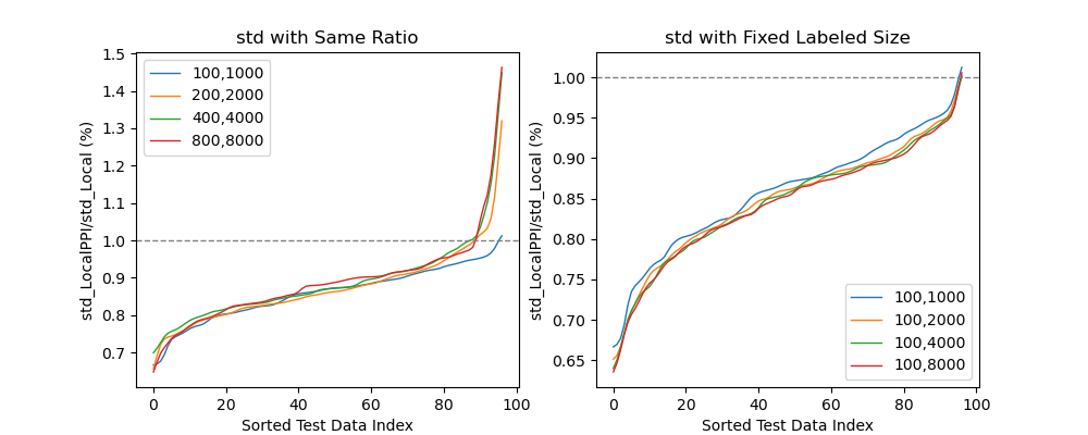
By dropping several NaN (Not a Number) data, 21597 instances are left, and we split them into train dataset (10,000 instances), labeled dataset (1,500 instances), unlabeled dataset (10,000 instances) and test dataset (97 instances). Under the paradigm of prediction-powered inference, we trained a model under a train dataset and gave predictions to the labeled dataset and the unlabeled dataset. For the sample size of (un)labeled dataset, we tested with same ratio 10 for four times: (100, 1000), (200, 2000), (400, 4000), (800, 8000) and with fixed labeled size 100 for four times: (100, 1000), (100, 2000), (100, 4000), (100, 8000). The mean absolute error (MAE) and the standard error of the estimations are contrasted.

Refer to caption
Figure 5: Deduction of Mean Absolute Error
Refer to caption
Figure 6: Deduction of Standard Error of Estimation

For the 97 instances within the test dataset, each instance was designated as the target point. The corresponding segments of the labeled and unlabeled datasets were sampled, followed by performing inference 100 times under sampling data. The mean absolute error (MAE) and standard error (S.E.) for each target point were calculated. Subsequently, the 97 instances in the test dataset were ranked and the deduction of MAE and SE under the prediction model were compared, as illustrated in Figures 5 and 6.

From Figure 5, it is observed that for each target data point, the mean absolute errors (MAEs) of local multivariable inference and local PPI exhibit comparable performance. An increment in the size of the unlabeled dataset results in a marginal increase in the absolute error. This escalation in the performance of MAEs, despite maintaining a constant unlabeled-labeled ratio, can probably be attributed to the suboptimal performance of the underlying model.

In Figure 6, more than 90% of the instances demonstrate an improvement in variance performance when maintaining a fixed unlabeled-labeled ratio. Additionally, nearly all instances exhibit more stable estimations with a fixed labeled dataset size under the technique of prediction-powered inference. Furthermore, an increase in the unlabeled dataset size, while keeping the labeled dataset size constant, augments the stability of performance as corroborated by theoretical analysis. Actually, the Mean Squared Error (MSE) of the same target point has the same expression as the standard error, which has the same conclusion.

It is worth mentioning that due to the lack of training set, the XGBoost predictor F𝐹F still suffers from a relatively high error. But this shortcoming does not significantly influence the performance of prediction-powered inference, because of the debias operations taken by rectifier ΔΔ\Delta.

In conclusion, compared to the local multivariable regression, the local prediction-powered inference can give a more stable estimation without the higher cost of absolute error.

4.3 Air Quality Inference

In this real-data experiment, we focus on a dataset of hourly air quality in India. Twenty monitoring stations give over 200,000 records from 2015 to 2020 with 19 observable variables including particulate pollutants, nitrogen oxides, combustion gaseous pollutants, sulfur compounds and volatile organic compounds. The AQI (Air Quality Index) has a complex calculation method related to the above variables which can be recognized as the potential function m​(x)𝑚𝑥m(x). Thus, our target is to use various pollutant contents to estimate AQI.

The data were compiled from the website of the Central Pollution Control Board (CPCB) https://cpcb.nic.in/, the official authority of the Government of India, and the complete version is available on the Kaggle website https://www.kaggle.com/datasets/rohanrao/air-quality-data-in-india.

In our configuration, the dataset is partitioned into training, testing, labeled, and unlabeled subsets. The test dataset comprises records from a particular station, kept aside for evaluation purposes. The training dataset encompasses numerous records that may contain missing data, which, although not useful for inference, contribute to the effective training of the XGBoost model. The unlabeled dataset includes records where some equipment may have incomplete or inaccurate data, resulting in the absence of labels. Conversely, the labeled dataset contains complete and accurate data required for the implementation of the local PPI method.

For each target point in the test dataset, we perform bootstrapping 100 times by sampling 2,000 instances from the labeled dataset and 20,000 instances from the unlabeled dataset, respectively. Applying the bandwidth h=0.7ℎ0.7h=0.7 and PCA operations to the pollution content clusters, local prediction-powered inference based on the 5-variable demonstrates superior performance as Figure 7.

Refer to caption
(a)
Refer to caption
(b)
Figure 7: Comparison of Local Multivariable Regression and Local PPI

Figure 7(a) presents a comparison between local PPI and local multivariable inference for each target point. When the arrows point to the right, the PPI method reduces the standard deviation of the estimation for the respective target point; and the arrows pointing upward indicate that the PPI method decreases the mean squared error of the estimation for the corresponding target point. Conversely, directions towards the left and downward signify high volatility and low accuracy. The overall statistic of arrow plot is listed before in Figure 1(b).

Figure 7(b) presents a comparison between local multivariable inference and local prediction-powered inference, using a combination of box plots and scatter plots to illustrate estimation standard deviation and mean squared error (MSE). The box plots reveal that the method on the right has a lower median standard deviation and a more compact interquartile range, indicating a reduction in variability compared to the method on the left. This suggests a more consistent performance in the estimations. The scatter plots, where the height of each point corresponds to its standard deviation and the horizontal distance from the box plot’s central line reflects its MSE, show that despite the reduced variance in the second method, there is no noticeable increase in error. Both methods maintain similar distributions of MSE, with points scattered relatively evenly around the central line. In general, the method on the right demonstrates improved stability by reducing the variance of the estimate without introducing higher errors, making it more effective in maintaining accuracy.

Broadly speaking, our innovative approach harnesses the power of the unlabeled dataset in conjunction with models adeptly trained on missing-feature data. This synergy not only significantly bolsters the predictive prowess of local multivariable inference, enhancing its stability to a remarkable degree, but does so without ever sacrificing accuracy.

5 Conclusions

The simulation experiment and the real data trial proved that local prediction-powered inference can reduce volatility of the estimation, especially when the sample size of the labeled dataset is limited.

In contrast to the evaluation of traditional inference methodologies, our analysis focuses on the theoretical performance at a specific target point, i.e., locally rather than across global conditions. Given an expected error of equal equality, the predictor F𝐹F demonstrably yields a lower variance, as substantiated by theoretical proof. Furthermore, the confidence interval retains the same order of magnitude irrespective of bias adjustment. Coverage probabilities are validated via elementary algebra in one dimension and through the application of an introduced biased Beta distribution in multiple dimensions.

The improvement of local prediction-powered inference in contrast of simply applying prediction-powered inference, includes:

  • •

    The computation of (sub)gradients of PPI is replaced by explicit solution expressed by the matrix of features, weights and response values, which improves the computation efficiency;

  • •

    The dependence of components can be described by the inverse of matrix of features, in contrast of the independence of classical PPI approach.

There are also several open problems of prediction-powered inference technique, including:

  • •

    The criterion of good predictor F𝐹F which to determine whether use the PPI or not;

  • •

    The general paradigm of PPI;

  • •

    The implementation of other non-linear and no-explicit-solution optimization problem.

Notwithstanding, local prediction-powered inference offers a methodology to enhance the stability of estimations for a specified local target. Despite the constraints in the size of the labeled dataset, our approach remains effective. Furthermore, local prediction-powered inference can be employed in high-cost design scenarios with commendable simulation techniques, or in social investigation issues that can be addressed through alternative investments.

Acknowledgments

Yanwu Gu’s research was partially supported by HKPFS PF22-69747. Dong Xia’s research was partially supported by Hong Kong RGC grant GRF 16300121.

References

  • [1] Abraham Savitzky and Marcel JE Golay. Smoothing and differentiation of data by simplified least squares procedures. Analytical chemistry, 36(8):1627–1639, 1964.
  • [2] William S Cleveland. Robust locally weighted regression and smoothing scatterplots. Journal of the American statistical association, 74(368):829–836, 1979.
  • [3] William S Cleveland and Susan J Devlin. Locally weighted regression: an approach to regression analysis by local fitting. Journal of the American statistical association, 83(403):596–610, 1988.
  • [4] Cheng-Kuan Lin and Heiu-Jou Shaw. Feature-based estimation of preliminary costs in shipbuilding. Ocean Engineering, 144:305–319, 2017.
  • [5] Zhan-Qian Lu. Multivariate locally weighted polynomial fitting and partial derivative estimation. journal of multivariate analysis, 59(2):187–205, 1996.
  • [6] Anastasios N. Angelopoulos, Stephen Bates, Clara Fannjiang, Michael I. Jordan, and Tijana Zrnic. Prediction-powered inference. Science, 382(6671):669–674, 2023.
  • [7] Clive Loader. Local regression and likelihood. Springer Science & Business Media, 2006.
  • [8] Jianqing Fan, Irène Gijbels, Tien-Chung Hu, and Li-Shan Huang. A study of variable bandwidth selection for local polynomial regression. Statistica Sinica, pages 113–127, 1996.
  • [9] Elias Søvik Gunnarsson, Håkon Ramon Isern, Aristidis Kaloudis, Morten Risstad, Benjamin Vigdel, and Sjur Westgaard. Prediction of realized volatility and implied volatility indices using ai and machine learning: A review. International Review of Financial Analysis, page 103221, 2024.
  • [10] Mingxuan Cai, Jiashun Xiao, Shunkang Zhang, Xiang Wan, Hongyu Zhao, Gang Chen, and Can Yang. A unified framework for cross-population trait prediction by leveraging the genetic correlation of polygenic traits. The American Journal of Human Genetics, 108(4):632–655, 2021.
  • [11] Elizbar A Nadaraya. On estimating regression. Theory of Probability & Its Applications, 9(1):141–142, 1964.
  • [12] Geoffrey S Watson. Smooth regression analysis. Sankhyā: The Indian Journal of Statistics, Series A, pages 359–372, 1964.
  • [13] Theo Gasser and Hans-Georg Müller. Kernel estimation of regression functions. In Smoothing Techniques for Curve Estimation: Proceedings of a Workshop held in Heidelberg, April 2–4, 1979, pages 23–68. Springer, 1979.
  • [14] Jianqing Fan. Local linear regression smoothers and their minimax efficiencies. The annals of Statistics, pages 196–216, 1993.
  • [15] Theo Gasser, Hans-Georg Muller, and Volker Mammitzsch. Kernels for nonparametric curve estimation. Journal of the Royal Statistical Society. Series B (Methodological), pages 238–252, 1985.
  • [16] Jianqing Fan, Theo Gasser, Irène Gijbels, Michael Brockmann, and Joachim Engel. Local polynomial regression: Optimal kernels and asymptotic minimax efficiency. Annals of the Institute of Statistical Mathematics, 49:79–99, 1997.
  • [17] Jianqing Fan and Irene Gijbels. Data-driven bandwidth selection in local polynomial fitting: variable bandwidth and spatial adaptation. Journal of the Royal Statistical Society: Series B (Methodological), 57(2):371–394, 1995.
  • [18] David Ruppert, Simon J Sheather, and Matthew P Wand. An effective bandwidth selector for local least squares regression. Journal of the American Statistical Association, 90(432):1257–1270, 1995.
  • [19] Siruo Wang, Tyler H McCormick, and Jeffrey T Leek. Methods for correcting inference based on outcomes predicted by machine learning. Proceedings of the National Academy of Sciences, 117(48):30266–30275, 2020.
  • [20] James M Robins, Andrea Rotnitzky, and Lue Ping Zhao. Estimation of regression coefficients when some regressors are not always observed. Journal of the American statistical Association, 89(427):846–866, 1994.
  • [21] Anru R. Zhang, Lawrence D. Brown, and T. Tony Cai. Semi-supervised inference: General theory and estimation of means. The Annals of Statistics, 2016.
  • [22] Abhishek Chakrabortty, Guorong Dai, and Raymond J Carroll. Semi-supervised quantile estimation: Robust and efficient inference in high dimensional settings. arXiv preprint arXiv:2201.10208, 2022.
  • [23] David Azriel, Lawrence D Brown, Michael Sklar, Richard Berk, Andreas Buja, and Linda Zhao. Semi-supervised linear regression. Journal of the American Statistical Association, 117(540):2238–2251, 2022.
  • [24] Abhishek Chakrabortty and Tianxi Cai. Efficient and adaptive linear regression in semi-supervised settings. The Annals of Statistics, 46(4):1541 – 1572, 2018.
  • [25] Yuqian Zhang and Jelena Bradic. High-dimensional semi-supervised learning: in search of optimal inference of the mean. Biometrika, 109(2):387–403, 2022.
  • [26] Shanshan Song, Yuanyuan Lin, and Yong Zhou. A general m-estimation theory in semi-supervised framework. Journal of the American Statistical Association, 119(546):1065–1075, 2024.
  • [27] Anastasios N Angelopoulos, John C Duchi, and Tijana Zrnic. Ppi++: Efficient prediction-powered inference. arXiv preprint arXiv:2311.01453, 2023.
  • [28] Jeffrey T Leek and John D Storey. Capturing heterogeneity in gene expression studies by surrogate variable analysis. PLoS genetics, 3(9):e161, 2007.
  • [29] Davide Risso, John Ngai, Terence P Speed, and Sandrine Dudoit. Normalization of rna-seq data using factor analysis of control genes or samples. Nature biotechnology, 32(9):896–902, 2014.
  • [30] Gordon K Smyth. Limma: linear models for microarray data. In Bioinformatics and computational biology solutions using R and Bioconductor, pages 397–420. Springer, 2005.

Appendix A Proof of Theorems

A.1 Proof of Theorem 1

Proof.

First, we decompose the expression of error as

𝔼​(θ^(n)−θ∗|X1,…,Xn)=𝔼​(θ^(n)|X1,…,Xn)−θ∗=(𝐗𝐖𝐗T)−1​𝐗𝐖​(𝐌−𝐗T​β)=diag​{1,h−1​Ip}​Sn−1​Rn,𝔼subscript^𝜃𝑛conditionalsuperscript𝜃subscript𝑋1…subscript𝑋𝑛𝔼conditionalsubscript^𝜃𝑛subscript𝑋1…subscript𝑋𝑛superscript𝜃superscriptsuperscript𝐗𝐖𝐗𝑇1𝐗𝐖𝐌superscript𝐗𝑇𝛽diag1superscriptℎ1subscript𝐼𝑝superscriptsubscript𝑆𝑛1subscript𝑅𝑛\begin{split}\mathbb{E}(\widehat{\theta}_{(n)}-\theta^{*}|X_{1},\dots,X_{n})&=\mathbb{E}(\widehat{\theta}_{(n)}|X_{1},\dots,X_{n})-\theta^{*}\\ &=(\mathbf{X}\mathbf{W}\mathbf{X}^{T})^{-1}\mathbf{X}\mathbf{W}(\mathbf{M}-\mathbf{X}^{T}\beta)\\ &=\text{diag}\{1,h^{-1}I_{p}\}S_{n}^{-1}R_{n},\end{split}

where

𝐌=(m​(X1)⋯m​(Xn))T,Sn=1n​∑i=1nh−p​(1Xi−xh)​(1Xi−xh)​K​(Xi−xh),Rn=1n​∑i=1n(1Xi−xh)​[m​(Xi)−m​(x)−∇mT​(x)​(Xi−x)]​h−p​K​(Xi−xh).formulae-sequence𝐌superscriptmatrix𝑚subscript𝑋1⋯𝑚subscript𝑋𝑛𝑇formulae-sequencesubscript𝑆𝑛1𝑛superscriptsubscript𝑖1𝑛superscriptℎ𝑝matrix1subscript𝑋𝑖𝑥ℎmatrix1subscript𝑋𝑖𝑥ℎ𝐾subscript𝑋𝑖𝑥ℎsubscript𝑅𝑛1𝑛superscriptsubscript𝑖1𝑛matrix1subscript𝑋𝑖𝑥ℎdelimited-[]𝑚subscript𝑋𝑖𝑚𝑥∇superscript𝑚𝑇𝑥subscript𝑋𝑖𝑥superscriptℎ𝑝𝐾subscript𝑋𝑖𝑥ℎ\begin{split}\mathbf{M}&=\left(\begin{matrix}m(X_{1})&\cdots&m(X_{n})\end{matrix}\right)^{T},\\ S_{n}&=\frac{1}{n}\sum_{i=1}^{n}h^{-p}\left(\begin{matrix}1\\ \frac{X_{i}-x}{h}\end{matrix}\right)\left(\begin{matrix}1&\frac{X_{i}-x}{h}\end{matrix}\right)K\left(\frac{X_{i}-x}{h}\right),\\ R_{n}&=\frac{1}{n}\sum_{i=1}^{n}\left(\begin{matrix}1\\ \frac{X_{i}-x}{h}\end{matrix}\right)\left[m(X_{i})-m(x)-\nabla m^{T}(x)(X_{i}-x)\right]h^{-p}K\left(\frac{X_{i}-x}{h}\right).\\ \end{split}

To estimate Sn−1superscriptsubscript𝑆𝑛1S_{n}^{-1} and Rnsubscript𝑅𝑛R_{n}, we use the Central Limit Theorem and we have

𝔼​Sn=∫h−p​(1X1−xh)​(1X1−xh)​K​(X1−xh)​f​(X1)​𝑑X1=∫(1u)​(1u)​K​(u)​f​(x+h​u)​𝑑u:=A​(h),n​hp​(Sn−A​(h))=Op​(1),Sn=A​(h)+Op​({n​hp}−1/2).formulae-sequence𝔼subscript𝑆𝑛superscriptℎ𝑝matrix1subscript𝑋1𝑥ℎmatrix1subscript𝑋1𝑥ℎ𝐾subscript𝑋1𝑥ℎ𝑓subscript𝑋1differential-dsubscript𝑋1matrix1𝑢matrix1𝑢𝐾𝑢𝑓𝑥ℎ𝑢differential-d𝑢assign𝐴ℎformulae-sequence𝑛superscriptℎ𝑝subscript𝑆𝑛𝐴ℎsubscript𝑂𝑝1subscript𝑆𝑛𝐴ℎsubscript𝑂𝑝superscript𝑛superscriptℎ𝑝12\begin{split}\mathbb{E}S_{n}&=\int h^{-p}\left(\begin{matrix}1\\ \frac{X_{1}-x}{h}\end{matrix}\right)\left(\begin{matrix}1&\frac{X_{1}-x}{h}\end{matrix}\right)K\left(\frac{X_{1}-x}{h}\right)f(X_{1})dX_{1}\\ &=\int\left(\begin{matrix}1\\ u\end{matrix}\right)\left(\begin{matrix}1&u\end{matrix}\right)K(u)f(x+hu)du:=A(h),\\ \sqrt{nh^{p}}(S_{n}-A(h))&=O_{p}(1),\\ S_{n}&=A(h)+O_{p}(\{nh^{p}\}^{-1/2}).\end{split}

Since

Sn−1=A−1​(h)+Op​({n​hp}−1/2),superscriptsubscript𝑆𝑛1superscript𝐴1ℎsubscript𝑂𝑝superscript𝑛superscriptℎ𝑝12S_{n}^{-1}=A^{-1}(h)+O_{p}(\{nh^{p}\}^{-1/2}),

and

A​(h)=∫(1uTuu​uT)​K​(u)​f​(x+h​u)​𝑑u=f​(x)​∫(1uTuu​uT)​K​(u)​𝑑u+h​∫(1uTuu​uT)​∇f​(x)T​u​K​(u)​𝑑u+O​(h2)=(f​(x)h​μ2​∇f​(x)Th​μ2​∇f​(x)μ2​f​(x)​Ip)+O​(h2),𝐴ℎmatrix1superscript𝑢𝑇𝑢𝑢superscript𝑢𝑇𝐾𝑢𝑓𝑥ℎ𝑢differential-d𝑢𝑓𝑥matrix1superscript𝑢𝑇𝑢𝑢superscript𝑢𝑇𝐾𝑢differential-d𝑢ℎmatrix1superscript𝑢𝑇𝑢𝑢superscript𝑢𝑇∇𝑓superscript𝑥𝑇𝑢𝐾𝑢differential-d𝑢𝑂superscriptℎ2matrix𝑓𝑥ℎsubscript𝜇2∇𝑓superscript𝑥𝑇ℎsubscript𝜇2∇𝑓𝑥subscript𝜇2𝑓𝑥subscript𝐼𝑝𝑂superscriptℎ2\begin{split}A(h)&=\int\left(\begin{matrix}1&u^{T}\\ u&uu^{T}\end{matrix}\right)K(u)f(x+hu)du\\ &=f(x)\int\left(\begin{matrix}1&u^{T}\\ u&uu^{T}\end{matrix}\right)K(u)du+h\int\left(\begin{matrix}1&u^{T}\\ u&uu^{T}\end{matrix}\right)\nabla f(x)^{T}uK(u)du+O(h^{2})\\ &=\left(\begin{matrix}f(x)&h\mu_{2}\nabla f(x)^{T}\\ h\mu_{2}\nabla f(x)&\mu_{2}f(x)I_{p}\end{matrix}\right)+O(h^{2}),\end{split}

using the inverse matrix formula

(ABTBD)−1=(E−1−E−1​FT−F​E−1D−1+F​E−1​FT),superscriptmatrix𝐴superscript𝐵𝑇𝐵𝐷1matrixsuperscript𝐸1superscript𝐸1superscript𝐹𝑇𝐹superscript𝐸1superscript𝐷1𝐹superscript𝐸1superscript𝐹𝑇\left(\begin{matrix}A&B^{T}\\ B&D\end{matrix}\right)^{-1}=\left(\begin{matrix}E^{-1}&-E^{-1}F^{T}\\ -FE^{-1}&D^{-1}+FE^{-1}F^{T}\end{matrix}\right),

where E=A−BT​D−1​B,F=D−1​Bformulae-sequence𝐸𝐴superscript𝐵𝑇superscript𝐷1𝐵𝐹superscript𝐷1𝐵E=A-B^{T}D^{-1}B,F=D^{-1}B, we have

E=f​(x)−h2​μ2f​(x)​∇f​(x)T​∇f​(x),F=hf​(x)​∇f​(x).formulae-sequence𝐸𝑓𝑥superscriptℎ2subscript𝜇2𝑓𝑥∇𝑓superscript𝑥𝑇∇𝑓𝑥𝐹ℎ𝑓𝑥∇𝑓𝑥\begin{split}E&=f(x)-\frac{h^{2}\mu_{2}}{f(x)}\nabla f(x)^{T}\nabla f(x),\\ F&=\frac{h}{f(x)}\nabla f(x).\\ \end{split}

And then we conclude that

A−1​(h)=(E−1−E−1​FT−F​E−1D−1+F​E−1​FT)=(1/f​(x)+O​(h2)−h/f2​(x)⋅∇f​(x)T+O​(h3)−h/f2​(x)⋅∇f​(x)+O​(h3)1/(μ2​f​(x))​I+O​(h2))=1f​(x)​(1−h/f​(x)⋅∇f​(x)T−h/f​(x)⋅∇f​(x)1/μ2⋅Ip)+O​(h2).superscript𝐴1ℎmatrixsuperscript𝐸1superscript𝐸1superscript𝐹𝑇𝐹superscript𝐸1superscript𝐷1𝐹superscript𝐸1superscript𝐹𝑇matrix1𝑓𝑥𝑂superscriptℎ2⋅ℎsuperscript𝑓2𝑥∇𝑓superscript𝑥𝑇𝑂superscriptℎ3⋅ℎsuperscript𝑓2𝑥∇𝑓𝑥𝑂superscriptℎ31subscript𝜇2𝑓𝑥𝐼𝑂superscriptℎ21𝑓𝑥matrix1⋅ℎ𝑓𝑥∇𝑓superscript𝑥𝑇⋅ℎ𝑓𝑥∇𝑓𝑥⋅1subscript𝜇2subscript𝐼𝑝𝑂superscriptℎ2\begin{split}A^{-1}(h)&=\left(\begin{matrix}E^{-1}&-E^{-1}F^{T}\\ -FE^{-1}&D^{-1}+FE^{-1}F^{T}\end{matrix}\right)\\ &=\left(\begin{matrix}1/f(x)+O(h^{2})&-h/f^{2}(x)\cdot\nabla f(x)^{T}+O(h^{3})\\ -h/f^{2}(x)\cdot\nabla f(x)+O(h^{3})&1/(\mu_{2}f(x))I+O(h^{2})\\ \end{matrix}\right)\\ &=\frac{1}{f(x)}\left(\begin{matrix}1&-h/f(x)\cdot\nabla f(x)^{T}\\ -h/f(x)\cdot\nabla f(x)&1/\mu_{2}\cdot I_{p}\\ \end{matrix}\right)+O(h^{2}).\end{split} (21)

For the residual term, using the Assumption 2 (ii) to get

𝔼​Rn=∫(1X1−xh)​[m​(X1)−m​(x)−∇mT​(x)​(X1−x)]​h−p​K​(X1−xh)​f​(X1)​𝑑X1=∫(1u)​[m​(x+u​h)−m​(x)−h​∇mT​(x)​u]​K​(u)​f​(x+u​h)​𝑑u=∫(1u)​[h22​uT​∇2m​(x)​u+h33!​Dm3​(x,u)]​K​(u)​f​(x+u​h)​𝑑u,𝔼subscript𝑅𝑛matrix1subscript𝑋1𝑥ℎdelimited-[]𝑚subscript𝑋1𝑚𝑥∇superscript𝑚𝑇𝑥subscript𝑋1𝑥superscriptℎ𝑝𝐾subscript𝑋1𝑥ℎ𝑓subscript𝑋1differential-dsubscript𝑋1matrix1𝑢delimited-[]𝑚𝑥𝑢ℎ𝑚𝑥ℎ∇superscript𝑚𝑇𝑥𝑢𝐾𝑢𝑓𝑥𝑢ℎdifferential-d𝑢matrix1𝑢delimited-[]superscriptℎ22superscript𝑢𝑇superscript∇2𝑚𝑥𝑢superscriptℎ33superscriptsubscript𝐷𝑚3𝑥𝑢𝐾𝑢𝑓𝑥𝑢ℎdifferential-d𝑢\begin{split}\mathbb{E}R_{n}&=\int\left(\begin{matrix}1\\ \frac{X_{1}-x}{h}\end{matrix}\right)\left[m(X_{1})-m(x)-\nabla m^{T}(x)(X_{1}-x)\right]h^{-p}K\left(\frac{X_{1}-x}{h}\right)f(X_{1})dX_{1}\\ &=\int\left(\begin{matrix}1\\ u\end{matrix}\right)\left[m(x+uh)-m(x)-h\nabla m^{T}(x)u\right]K(u)f(x+uh)du\\ &=\int\left(\begin{matrix}1\\ u\end{matrix}\right)\left[\frac{h^{2}}{2}u^{T}\nabla^{2}m(x)u+\frac{h^{3}}{3!}D_{m}^{3}(x,u)\right]K(u)f(x+uh)du,\\ \end{split}

Do Taylor expansion to f​(x+u​h)𝑓𝑥𝑢ℎf(x+uh) and we conclude that

∫uT​∇2m​(x)​u​K​(u)​f​(x+u​h)​𝑑u=f​(x)​μ2​Tr​(∇2m​(x))+O​(h2),∫Dm3​(x,u)​K​(u)​f​(x+u​h)​𝑑u=O​(h),(𝔼​Rn)1=12​h2​f​(x)​μ2​Tr​(∇2m​(x))+O​(h4)∫u​[uT​∇2m​(x)​u]​K​(u)​f​(x+u​h)=h​∫u​[uT​∇2m​(x)​u]​∇f​(x)T​u​K​(u)​𝑑u+O​(h3),∫u​Dm3​(x,u)​K​(u)​f​(x+u​h)​𝑑u=f​(x)​∫u​Dm3​(x,u)​K​(u)​𝑑u+O​(h3),(𝔼​Rn)2:p+1=12​h3​∫u​[uT​∇2m​(x)​u]​∇f​(x)T​u​K​(u)​𝑑u+13!​f​(x)​h3​∫u​Dm3​(x,u)​K​(u)​𝑑u+O​(h5).formulae-sequenceformulae-sequencesuperscript𝑢𝑇superscript∇2𝑚𝑥𝑢𝐾𝑢𝑓𝑥𝑢ℎdifferential-d𝑢𝑓𝑥subscript𝜇2Trsuperscript∇2𝑚𝑥𝑂superscriptℎ2formulae-sequencesuperscriptsubscript𝐷𝑚3𝑥𝑢𝐾𝑢𝑓𝑥𝑢ℎdifferential-d𝑢𝑂ℎsubscript𝔼subscript𝑅𝑛112superscriptℎ2𝑓𝑥subscript𝜇2Trsuperscript∇2𝑚𝑥𝑂superscriptℎ4𝑢delimited-[]superscript𝑢𝑇superscript∇2𝑚𝑥𝑢𝐾𝑢𝑓𝑥𝑢ℎℎ𝑢delimited-[]superscript𝑢𝑇superscript∇2𝑚𝑥𝑢∇𝑓superscript𝑥𝑇𝑢𝐾𝑢differential-d𝑢𝑂superscriptℎ3formulae-sequence𝑢superscriptsubscript𝐷𝑚3𝑥𝑢𝐾𝑢𝑓𝑥𝑢ℎdifferential-d𝑢𝑓𝑥𝑢superscriptsubscript𝐷𝑚3𝑥𝑢𝐾𝑢differential-d𝑢𝑂superscriptℎ3subscript𝔼subscript𝑅𝑛:2𝑝112superscriptℎ3𝑢delimited-[]superscript𝑢𝑇superscript∇2𝑚𝑥𝑢∇𝑓superscript𝑥𝑇𝑢𝐾𝑢differential-d𝑢13𝑓𝑥superscriptℎ3𝑢superscriptsubscript𝐷𝑚3𝑥𝑢𝐾𝑢differential-d𝑢𝑂superscriptℎ5\begin{split}\int u^{T}\nabla^{2}m(x)uK(u)f(x+uh)du=&f(x)\mu_{2}\text{Tr}(\nabla^{2}m(x))+O(h^{2}),\\ \int D_{m}^{3}(x,u)K(u)f(x+uh)du=&O(h),\\ (\mathbb{E}R_{n})_{1}=&\frac{1}{2}h^{2}f(x)\mu_{2}\text{Tr}(\nabla^{2}m(x))+O(h^{4})\\ \int u[u^{T}\nabla^{2}m(x)u]K(u)f(x+uh)=&h\int u[u^{T}\nabla^{2}m(x)u]\nabla f(x)^{T}uK(u)du+O(h^{3}),\\ \int uD_{m}^{3}(x,u)K(u)f(x+uh)du=&f(x)\int uD_{m}^{3}(x,u)K(u)du+O(h^{3}),\\ (\mathbb{E}R_{n})_{2:p+1}=&\frac{1}{2}h^{3}\int u[u^{T}\nabla^{2}m(x)u]\nabla f(x)^{T}uK(u)du\\ &+\frac{1}{3!}f(x)h^{3}\int uD_{m}^{3}(x,u)K(u)du+O(h^{5}).\\ \end{split}

Denote that b​(m)=∫u​Dm3​(x,u)​K​(u)​𝑑u𝑏𝑚𝑢superscriptsubscript𝐷𝑚3𝑥𝑢𝐾𝑢differential-d𝑢b(m)=\int uD_{m}^{3}(x,u)K(u)du, b1​(m)=∫u​[uT​∇2m​(x)​u]​∇f​(x)T​u​K​(u)​𝑑u−μ22​∇f​(x)​Tr​(∇2m​(x))subscript𝑏1𝑚𝑢delimited-[]superscript𝑢𝑇superscript∇2𝑚𝑥𝑢∇𝑓superscript𝑥𝑇𝑢𝐾𝑢differential-d𝑢superscriptsubscript𝜇22∇𝑓𝑥Trsuperscript∇2𝑚𝑥b_{1}(m)=\int u[u^{T}\nabla^{2}m(x)u]\nabla f(x)^{T}uK(u)du-\mu_{2}^{2}\nabla f(x)\text{Tr}(\nabla^{2}m(x)), and combine the above conclusions:

𝔼​(θ^(n)−θ|X1,…,Xn)=diag​{1,h−1​Ip}​Sn−1​Rn=diag​{1,h−1​Ip}​(A​(h)−1+O​({n​hp}−1/2))​Rn=(1h−1​Ip)​{(1f​(x)−hf2​(x)​∇f​(x)T−hf2​(x)​∇f​(x)1μ2​f​(x)​Ip)+O​(h2)+O​({n​hp}−1/2)}⋅(12​h2​f​(x)​μ2​Tr​(∇2m​(x))+O​(h4)12​h3​∫u​[uT​∇m​(x)​u]​∇f​(x)T​u​K​(u)​𝑑u+13!​f​(x)​h3​∫u​Dm​(x,u)​K​(u)​𝑑u+O​(h5))=(12​h2​f​(x)​μ2​Tr​(∇2m​(x))+O​(h4)+O​(n−1/2​h2−p/2)h22​μ2​f​(x)​b1​(m)+h23!​μ2​b​(m)+O​(h4)+O​(n−1/2​n2−p/2))=h2​(12​f​(x)​μ2​Tr​(∇2m​(x))12​μ2​f​(x)​b1​(m)+13!​μ2​b​(m))+O​(h4)+O​(n−1/2​h2−p/2).𝔼subscript^𝜃𝑛conditional𝜃subscript𝑋1…subscript𝑋𝑛diag1superscriptℎ1subscript𝐼𝑝superscriptsubscript𝑆𝑛1subscript𝑅𝑛diag1superscriptℎ1subscript𝐼𝑝𝐴superscriptℎ1𝑂superscript𝑛superscriptℎ𝑝12subscript𝑅𝑛⋅matrix1missing-subexpressionsuperscriptℎ1subscript𝐼𝑝matrix1𝑓𝑥ℎsuperscript𝑓2𝑥∇𝑓superscript𝑥𝑇ℎsuperscript𝑓2𝑥∇𝑓𝑥1subscript𝜇2𝑓𝑥subscript𝐼𝑝𝑂superscriptℎ2𝑂superscript𝑛superscriptℎ𝑝12matrix12superscriptℎ2𝑓𝑥subscript𝜇2Trsuperscript∇2𝑚𝑥𝑂superscriptℎ412superscriptℎ3𝑢delimited-[]superscript𝑢𝑇∇𝑚𝑥𝑢∇𝑓superscript𝑥𝑇𝑢𝐾𝑢differential-d𝑢13𝑓𝑥superscriptℎ3𝑢subscript𝐷𝑚𝑥𝑢𝐾𝑢differential-d𝑢𝑂superscriptℎ5matrix12superscriptℎ2𝑓𝑥subscript𝜇2Trsuperscript∇2𝑚𝑥𝑂superscriptℎ4𝑂superscript𝑛12superscriptℎ2𝑝2superscriptℎ22subscript𝜇2𝑓𝑥subscript𝑏1𝑚superscriptℎ23subscript𝜇2𝑏𝑚𝑂superscriptℎ4𝑂superscript𝑛12superscript𝑛2𝑝2superscriptℎ2matrix12𝑓𝑥subscript𝜇2Trsuperscript∇2𝑚𝑥12subscript𝜇2𝑓𝑥subscript𝑏1𝑚13subscript𝜇2𝑏𝑚𝑂superscriptℎ4𝑂superscript𝑛12superscriptℎ2𝑝2\begin{split}&\mathbb{E}(\widehat{\theta}_{(n)}-\theta|X_{1},\dots,X_{n})\\ =&\text{diag}\{1,h^{-1}I_{p}\}S_{n}^{-1}R_{n}\\ =&\text{diag}\{1,h^{-1}I_{p}\}(A(h)^{-1}+O(\{nh^{p}\}^{-1/2}))R_{n}\\ =&\left(\begin{matrix}1\\ &h^{-1}I_{p}\end{matrix}\right)\left\{\left(\begin{matrix}\frac{1}{f(x)}&-\frac{h}{f^{2}(x)}\nabla f(x)^{T}\\ -\frac{h}{f^{2}(x)}\nabla f(x)&\frac{1}{\mu_{2}f(x)}I_{p}\end{matrix}\right)+O(h^{2})+O(\{nh^{p}\}^{-1/2})\right\}\\ &\cdot\left(\begin{matrix}\frac{1}{2}h^{2}f(x)\mu_{2}\text{Tr}(\nabla^{2}m(x))+O(h^{4})\\ \frac{1}{2}h^{3}\int u[u^{T}\nabla m(x)u]\nabla f(x)^{T}uK(u)du+\frac{1}{3!}f(x)h^{3}\int uD_{m}(x,u)K(u)du+O(h^{5})\end{matrix}\right)\\ =&\left(\begin{matrix}\frac{1}{2}h^{2}f(x)\mu_{2}\text{Tr}(\nabla^{2}m(x))+O(h^{4})+O(n^{-1/2}h^{2-p/2})\\ \frac{h^{2}}{2\mu_{2}f(x)}b_{1}(m)+\frac{h^{2}}{3!\mu_{2}}b(m)+O(h^{4})+O(n^{-1/2}n^{2-p/2})\end{matrix}\right)\\ =&h^{2}\left(\begin{matrix}\frac{1}{2}f(x)\mu_{2}\text{Tr}(\nabla^{2}m(x))\\ \frac{1}{2\mu_{2}f(x)}b_{1}(m)+\frac{1}{3!\mu_{2}}b(m)\end{matrix}\right)+O(h^{4})+O(n^{-1/2}h^{2-p/2}).\end{split}

For the covariance of θ^(n)subscript^𝜃𝑛\widehat{\theta}_{(n)} , we have

θ^(n)−θ∗=(𝐗𝐖𝐗T)−1​𝐗𝐖​(𝐌+ε−θ∗T​𝐗)=(1h−1​Ip)​Sn−1​Rn+(1h−1​Ip)​Sn−1​Zn,subscript^𝜃𝑛superscript𝜃superscriptsuperscript𝐗𝐖𝐗𝑇1𝐗𝐖𝐌𝜀superscript𝜃absent𝑇𝐗matrix1missing-subexpressionmissing-subexpressionsuperscriptℎ1subscript𝐼𝑝superscriptsubscript𝑆𝑛1subscript𝑅𝑛matrix1missing-subexpressionmissing-subexpressionsuperscriptℎ1subscript𝐼𝑝superscriptsubscript𝑆𝑛1subscript𝑍𝑛\begin{split}\widehat{\theta}_{(n)}-\theta^{*}&=(\mathbf{X}\mathbf{W}\mathbf{X}^{T})^{-1}\mathbf{X}\mathbf{W}(\mathbf{M}+\varepsilon-\theta^{*T}\mathbf{X})\\ &=\left(\begin{matrix}1&\\ &h^{-1}I_{p}\end{matrix}\right)S_{n}^{-1}R_{n}+\left(\begin{matrix}1&\\ &h^{-1}I_{p}\end{matrix}\right)S_{n}^{-1}Z_{n},\end{split}

which implies that

(1h​Ip)​(θ(n)∗−θ∗−(1h−1​Ip)​Sn−1​Rn)=Sn−1​Zn,matrix1missing-subexpressionmissing-subexpressionℎsubscript𝐼𝑝superscriptsubscript𝜃𝑛superscript𝜃matrix1missing-subexpressionmissing-subexpressionsuperscriptℎ1subscript𝐼𝑝superscriptsubscript𝑆𝑛1subscript𝑅𝑛superscriptsubscript𝑆𝑛1subscript𝑍𝑛\left(\begin{matrix}1&\\ &hI_{p}\end{matrix}\right)\left(\theta_{(n)}^{*}-\theta^{*}-\left(\begin{matrix}1&\\ &h^{-1}I_{p}\end{matrix}\right)S_{n}^{-1}R_{n}\right)=S_{n}^{-1}Z_{n},

where

Zn=1n​∑i=1n(1Xi−xh)​K​(Xi−xh)​εi.subscript𝑍𝑛1𝑛superscriptsubscript𝑖1𝑛matrix1subscript𝑋𝑖𝑥ℎ𝐾subscript𝑋𝑖𝑥ℎsubscript𝜀𝑖Z_{n}=\frac{1}{n}\sum_{i=1}^{n}\left(\begin{matrix}1\\ \frac{X_{i}-x}{h}\end{matrix}\right)K\left(\frac{X_{i}-x}{h}\right)\varepsilon_{i}.

By CLT, we simply get that

Zn→dN​(0,σ2n​hp​f​(x)​(J0J2​Ip)).subscript→𝑑subscript𝑍𝑛𝑁0superscript𝜎2𝑛superscriptℎ𝑝𝑓𝑥matrixsubscript𝐽0missing-subexpressionmissing-subexpressionsubscript𝐽2subscript𝐼𝑝Z_{n}\to_{d}N\left(0,\frac{\sigma^{2}}{nh^{p}}f(x)\left(\begin{matrix}J_{0}&\\ &J_{2}I_{p}\end{matrix}\right)\right).

Thus,

Sn−1​Zn→dN​(0,σ2n​hp​f​(x)​Sn−1​(J0J2​Ip)​Sn−1)=N​(0,σ2n​hp​f​(x)​{(J0J2μ22​h2​Ip)+O​(h2)+O​(n−1/2​h−p/2)})Cov​(θ^(n)|X1,…,Xn)=σ2n​hp​f​(x)​{(J0J2μ22​h2​Ip)+O​(h2)+O​(n−1/2​h−p/2)}.subscript→𝑑superscriptsubscript𝑆𝑛1subscript𝑍𝑛𝑁0superscript𝜎2𝑛superscriptℎ𝑝𝑓𝑥superscriptsubscript𝑆𝑛1matrixsubscript𝐽0missing-subexpressionmissing-subexpressionsubscript𝐽2subscript𝐼𝑝superscriptsubscript𝑆𝑛1𝑁0superscript𝜎2𝑛superscriptℎ𝑝𝑓𝑥matrixsubscript𝐽0missing-subexpressionmissing-subexpressionsubscript𝐽2superscriptsubscript𝜇22superscriptℎ2subscript𝐼𝑝𝑂superscriptℎ2𝑂superscript𝑛12superscriptℎ𝑝2Covconditionalsubscript^𝜃𝑛subscript𝑋1…subscript𝑋𝑛superscript𝜎2𝑛superscriptℎ𝑝𝑓𝑥matrixsubscript𝐽0missing-subexpressionmissing-subexpressionsubscript𝐽2superscriptsubscript𝜇22superscriptℎ2subscript𝐼𝑝𝑂superscriptℎ2𝑂superscript𝑛12superscriptℎ𝑝2\begin{split}S_{n}^{-1}Z_{n}&\to_{d}N\left(0,\frac{\sigma^{2}}{nh^{p}}f(x)S_{n}^{-1}\left(\begin{matrix}J_{0}&\\ &J_{2}I_{p}\end{matrix}\right)S_{n}^{-1}\right)\\ &=N\left(0,\frac{\sigma^{2}}{nh^{p}f(x)}\left\{\left(\begin{matrix}J_{0}&\\ &\frac{J_{2}}{\mu_{2}^{2}h^{2}}I_{p}\end{matrix}\right)+O(h^{2})+O(n^{-1/2}h^{-p/2})\right\}\right)\\ \text{Cov}(\widehat{\theta}_{(n)}|X_{1},\dots,X_{n})&=\frac{\sigma^{2}}{nh^{p}f(x)}\left\{\left(\begin{matrix}J_{0}&\\ &\frac{J_{2}}{\mu_{2}^{2}h^{2}}I_{p}\end{matrix}\right)+O(h^{2})+O(n^{-1/2}h^{-p/2})\right\}.\end{split}

∎

A.2 Proof of Theorem 2

Proof.

Decompose expected error of the estimation θ^(N)subscript^𝜃𝑁\widehat{\theta}_{{(N)}} as the following format

𝔼​(θ^(N)−θ∗|ℒ,𝒰)=𝔼​(θ^(N)|ℒ,𝒰)−θ∗=(𝐗~​𝐖~​𝐗~T)−1​𝐗~​𝐖~​(𝐌~−𝐗~T​θ∗)−(𝐗~​𝐖~​𝐗~T)−1​𝐗~​𝐖~​𝐫~+(𝐗𝐖𝐗T)−1​𝐗𝐖𝐫.𝔼subscript^𝜃𝑁conditionalsuperscript𝜃ℒ𝒰𝔼conditionalsubscript^𝜃𝑁ℒ𝒰superscript𝜃superscript~𝐗~𝐖superscript~𝐗𝑇1~𝐗~𝐖~𝐌superscript~𝐗𝑇superscript𝜃superscript~𝐗~𝐖superscript~𝐗𝑇1~𝐗~𝐖~𝐫superscriptsuperscript𝐗𝐖𝐗𝑇1𝐗𝐖𝐫\begin{split}\mathbb{E}(\hat{\theta}_{(N)}-\theta^{*}|\mathcal{L},\mathcal{U})&=\mathbb{E}(\hat{\theta}_{(N)}|\mathcal{L},\mathcal{U})-\theta^{*}\\ &=(\widetilde{\mathbf{X}}\widetilde{\mathbf{W}}\widetilde{\mathbf{X}}^{T})^{-1}\widetilde{\mathbf{X}}\widetilde{\mathbf{W}}(\widetilde{\mathbf{M}}-\widetilde{\mathbf{X}}^{T}\theta^{*})-(\widetilde{\mathbf{X}}\widetilde{\mathbf{W}}\widetilde{\mathbf{X}}^{T})^{-1}\widetilde{\mathbf{X}}\widetilde{\mathbf{W}}\widetilde{\mathbf{r}}+(\mathbf{X}{\mathbf{W}}{\mathbf{X}}^{T})^{-1}\mathbf{X}{\mathbf{W}}{\mathbf{r}}.\end{split}

We have (𝐗~​𝐖~​𝐗~T)−1​𝐗~​𝐖~​(𝐌~−𝐗~T​θ∗)→N​(BL​(x,h)+O​(h4)+O​(N−1/2​h2−p/2),σ2​O​(N−1​hp))→superscript~𝐗~𝐖superscript~𝐗𝑇1~𝐗~𝐖~𝐌superscript~𝐗𝑇superscript𝜃𝑁subscript𝐵𝐿𝑥ℎ𝑂superscriptℎ4𝑂superscript𝑁12superscriptℎ2𝑝2superscript𝜎2𝑂superscript𝑁1superscriptℎ𝑝(\widetilde{\mathbf{X}}\widetilde{\mathbf{W}}\widetilde{\mathbf{X}}^{T})^{-1}\widetilde{\mathbf{X}}\widetilde{\mathbf{W}}(\widetilde{\mathbf{M}}-\widetilde{\mathbf{X}}^{T}\theta^{*})\to N(B_{L}(x,h)+O(h^{4})+O(N^{-1/2}h^{2-p/2}),\sigma^{2}O(N^{-1}h^{p})). Then we need to derive the corresponding distribution of (𝐗𝐖𝐗T)−1​𝐗𝐖𝐫−(𝐗~​𝐖~​𝐗~T)−1​𝐗~​𝐖~​𝐫~superscriptsuperscript𝐗𝐖𝐗𝑇1𝐗𝐖𝐫superscript~𝐗~𝐖superscript~𝐗𝑇1~𝐗~𝐖~𝐫(\mathbf{X}{\mathbf{W}}{\mathbf{X}}^{T})^{-1}\mathbf{X}{\mathbf{W}}{\mathbf{r}}-(\widetilde{\mathbf{X}}\widetilde{\mathbf{W}}\widetilde{\mathbf{X}}^{T})^{-1}\widetilde{\mathbf{X}}\widetilde{\mathbf{W}}\widetilde{\mathbf{r}}.

(𝐗𝐖𝐗T)−1​𝐗𝐖𝐫−(𝐗~​𝐖~​𝐗~T)−1​𝐗~​𝐖~​𝐫~=(1h−1​Ip)​Sn−1​Rn(r)−(1h−1​Ip)​S~N−1​R~N(r)={(1h−1​Ip)​{(1f​(x)−hf2​(x)​∇f​(x)T−hf2​(x)​∇f​(x)1μ2​f​(x)​Ip)+O​(h2)+O​({n​hp}−1/2)}​Rn(r)}−{(1h−1​Ip)​{(1f​(x)−hf2​(x)​∇f​(x)T−hf2​(x)​∇f​(x)1μ2​f​(x)​Ip)+O​(h2)+O​({N​hp}−1/2)}​R~N(r)}.superscriptsuperscript𝐗𝐖𝐗𝑇1𝐗𝐖𝐫superscript~𝐗~𝐖superscript~𝐗𝑇1~𝐗~𝐖~𝐫matrix1missing-subexpressionmissing-subexpressionsuperscriptℎ1subscript𝐼𝑝superscriptsubscript𝑆𝑛1superscriptsubscript𝑅𝑛𝑟matrix1missing-subexpressionmissing-subexpressionsuperscriptℎ1subscript𝐼𝑝superscriptsubscript~𝑆𝑁1superscriptsubscript~𝑅𝑁𝑟matrix1missing-subexpressionsuperscriptℎ1subscript𝐼𝑝matrix1𝑓𝑥ℎsuperscript𝑓2𝑥∇𝑓superscript𝑥𝑇ℎsuperscript𝑓2𝑥∇𝑓𝑥1subscript𝜇2𝑓𝑥subscript𝐼𝑝𝑂superscriptℎ2𝑂superscript𝑛superscriptℎ𝑝12superscriptsubscript𝑅𝑛𝑟matrix1missing-subexpressionsuperscriptℎ1subscript𝐼𝑝matrix1𝑓𝑥ℎsuperscript𝑓2𝑥∇𝑓superscript𝑥𝑇ℎsuperscript𝑓2𝑥∇𝑓𝑥1subscript𝜇2𝑓𝑥subscript𝐼𝑝𝑂superscriptℎ2𝑂superscript𝑁superscriptℎ𝑝12superscriptsubscript~𝑅𝑁𝑟\begin{split}&(\mathbf{X}{\mathbf{W}}{\mathbf{X}}^{T})^{-1}\mathbf{X}{\mathbf{W}}{\mathbf{r}}-(\widetilde{\mathbf{X}}\widetilde{\mathbf{W}}\widetilde{\mathbf{X}}^{T})^{-1}\widetilde{\mathbf{X}}\widetilde{\mathbf{W}}\widetilde{\mathbf{r}}\\ =&\left(\begin{matrix}1&\\ &h^{-1}I_{p}\end{matrix}\right)S_{n}^{-1}R_{n}^{(r)}-\left(\begin{matrix}1&\\ &h^{-1}I_{p}\end{matrix}\right)\widetilde{S}_{N}^{-1}\widetilde{R}_{N}^{(r)}\\ =&\left\{\left(\begin{matrix}1\\ &h^{-1}I_{p}\end{matrix}\right)\left\{\left(\begin{matrix}\frac{1}{f(x)}&-\frac{h}{f^{2}(x)}\nabla f(x)^{T}\\ -\frac{h}{f^{2}(x)}\nabla f(x)&\frac{1}{\mu_{2}f(x)}I_{p}\end{matrix}\right)+O(h^{2})+O(\{nh^{p}\}^{-1/2})\right\}R_{n}^{(r)}\right\}\\ &-\left\{\left(\begin{matrix}1\\ &h^{-1}I_{p}\end{matrix}\right)\left\{\left(\begin{matrix}\frac{1}{f(x)}&-\frac{h}{f^{2}(x)}\nabla f(x)^{T}\\ -\frac{h}{f^{2}(x)}\nabla f(x)&\frac{1}{\mu_{2}f(x)}I_{p}\end{matrix}\right)+O(h^{2})+O(\{Nh^{p}\}^{-1/2})\right\}\widetilde{R}_{N}^{(r)}\right\}.\\ \end{split}

Since the expectation of Rn(r)superscriptsubscript𝑅𝑛𝑟R_{n}^{(r)} and RN(r)superscriptsubscript𝑅𝑁𝑟R_{N}^{(r)} are the same due to their definition

Rn(r)=1n​∑i=1nh−p​(1Xi−xh)​K​(Xi−xh)​[F​(Xi)−m​(Xi)],R~N(r)=1N​∑i=1Nh−p​(1X~i−xh)​K​(X~i−xh)​[F​(X~i)−m​(X~i)],𝔼​Rn(r)=∫(1u)​K​(u)​r​(x+u​h)​f​(x+u​h)​𝑑u=𝔼​R~N(r),formulae-sequencesuperscriptsubscript𝑅𝑛𝑟1𝑛superscriptsubscript𝑖1𝑛superscriptℎ𝑝matrix1subscript𝑋𝑖𝑥ℎ𝐾subscript𝑋𝑖𝑥ℎdelimited-[]𝐹subscript𝑋𝑖𝑚subscript𝑋𝑖formulae-sequencesuperscriptsubscript~𝑅𝑁𝑟1𝑁superscriptsubscript𝑖1𝑁superscriptℎ𝑝matrix1subscript~𝑋𝑖𝑥ℎ𝐾subscript~𝑋𝑖𝑥ℎdelimited-[]𝐹subscript~𝑋𝑖𝑚subscript~𝑋𝑖𝔼superscriptsubscript𝑅𝑛𝑟matrix1𝑢𝐾𝑢𝑟𝑥𝑢ℎ𝑓𝑥𝑢ℎdifferential-d𝑢𝔼superscriptsubscript~𝑅𝑁𝑟\begin{split}R_{n}^{(r)}&=\frac{1}{n}\sum_{i=1}^{n}h^{-p}\left(\begin{matrix}1\\ \frac{X_{i}-x}{h}\end{matrix}\right)K\left(\frac{X_{i}-x}{h}\right)[F(X_{i})-m(X_{i})],\\ \widetilde{R}_{N}^{(r)}&=\frac{1}{N}\sum_{i=1}^{N}h^{-p}\left(\begin{matrix}1\\ \frac{\widetilde{X}_{i}-x}{h}\end{matrix}\right)K\left(\frac{\widetilde{X}_{i}-x}{h}\right)[F(\widetilde{X}_{i})-m(\widetilde{X}_{i})],\\ \mathbb{E}R_{n}^{(r)}&=\int\left(\begin{matrix}1\\ u\end{matrix}\right)K(u)r(x+uh)f(x+uh)du=\mathbb{E}\widetilde{R}_{N}^{(r)},\end{split}

we derive the distribution of their difference as

N​nN+n​hp​(Rn(r)−R~N(r))→dN​(0,∫(1uTuu​uT)​K2​(u)​r​(x+u​h)​f​(x+u​h)​𝑑u).subscript→𝑑𝑁𝑛𝑁𝑛superscriptℎ𝑝superscriptsubscript𝑅𝑛𝑟superscriptsubscript~𝑅𝑁𝑟𝑁0matrix1superscript𝑢𝑇𝑢𝑢superscript𝑢𝑇superscript𝐾2𝑢𝑟𝑥𝑢ℎ𝑓𝑥𝑢ℎdifferential-d𝑢\sqrt{\frac{Nn}{N+n}h^{p}}(R_{n}^{(r)}-\widetilde{R}_{N}^{(r)})\to_{d}N\left(0,\int\left(\begin{matrix}1&u^{T}\\ u&uu^{T}\end{matrix}\right)K^{2}(u)r(x+uh)f(x+uh)du\right).

Consequently, the distribution of the rectifier Δ^^Δ\hat{\Delta} can be derived as

(𝐗𝐖𝐗T)−1​𝐗𝐖𝐫−(𝐗~​𝐖~​𝐗~T)−1​𝐗~​𝐖~​𝐫~={(1h−1​Ip)​{(1f​(x)−hf2​(x)​∇f​(x)T−hf2​(x)​∇f​(x)1μ2​f​(x)​Ip)+O​(h2)+O​({n​hp}−1/2)}​Rn(r)}−{(1h−1​Ip)​{(1f​(x)−hf2​(x)​∇f​(x)T−hf2​(x)​∇f​(x)1μ2​f​(x)​Ip)+O​(h2)+O​({N​hp}−1/2)}​R~N(r)}=(1h−1​Ip)​{1f​(x)​(2−hf​(x)​∇f​(x)T−hf​(x)​∇f​(x)1μ2​Ip)+O​(h2)}​(Rn(r)−R~N(r))+(1h−1​Ip)​Rn(r)​O​({n​hp}−1/2)=(1h−1​Ip)​{1f​(x)​(2−hf​(x)​∇f​(x)T−hf​(x)​∇f​(x)1μ2​Ip)+O​(h2)}​op​({n​hp}−1/2)+(1h−1​Ip)​(𝔼​Rn(r)+op​({n​hp}−1/2))​O​({n​hp}−1/2)=(1h−1​Ip)​(𝔼​Rn(r)+op​(1))​O​({n​hp}−1/2).superscriptsuperscript𝐗𝐖𝐗𝑇1𝐗𝐖𝐫superscript~𝐗~𝐖superscript~𝐗𝑇1~𝐗~𝐖~𝐫matrix1missing-subexpressionsuperscriptℎ1subscript𝐼𝑝matrix1𝑓𝑥ℎsuperscript𝑓2𝑥∇𝑓superscript𝑥𝑇ℎsuperscript𝑓2𝑥∇𝑓𝑥1subscript𝜇2𝑓𝑥subscript𝐼𝑝𝑂superscriptℎ2𝑂superscript𝑛superscriptℎ𝑝12superscriptsubscript𝑅𝑛𝑟matrix1missing-subexpressionsuperscriptℎ1subscript𝐼𝑝matrix1𝑓𝑥ℎsuperscript𝑓2𝑥∇𝑓superscript𝑥𝑇ℎsuperscript𝑓2𝑥∇𝑓𝑥1subscript𝜇2𝑓𝑥subscript𝐼𝑝𝑂superscriptℎ2𝑂superscript𝑁superscriptℎ𝑝12superscriptsubscript~𝑅𝑁𝑟matrix1missing-subexpressionsuperscriptℎ1subscript𝐼𝑝1𝑓𝑥matrix2ℎ𝑓𝑥∇𝑓superscript𝑥𝑇ℎ𝑓𝑥∇𝑓𝑥1subscript𝜇2subscript𝐼𝑝𝑂superscriptℎ2superscriptsubscript𝑅𝑛𝑟superscriptsubscript~𝑅𝑁𝑟matrix1missing-subexpressionsuperscriptℎ1subscript𝐼𝑝superscriptsubscript𝑅𝑛𝑟𝑂superscript𝑛superscriptℎ𝑝12matrix1missing-subexpressionsuperscriptℎ1subscript𝐼𝑝1𝑓𝑥matrix2ℎ𝑓𝑥∇𝑓superscript𝑥𝑇ℎ𝑓𝑥∇𝑓𝑥1subscript𝜇2subscript𝐼𝑝𝑂superscriptℎ2subscript𝑜𝑝superscript𝑛superscriptℎ𝑝12matrix1missing-subexpressionsuperscriptℎ1subscript𝐼𝑝𝔼superscriptsubscript𝑅𝑛𝑟subscript𝑜𝑝superscript𝑛superscriptℎ𝑝12𝑂superscript𝑛superscriptℎ𝑝12matrix1missing-subexpressionsuperscriptℎ1subscript𝐼𝑝𝔼superscriptsubscript𝑅𝑛𝑟subscript𝑜𝑝1𝑂superscript𝑛superscriptℎ𝑝12\begin{split}&(\mathbf{X}{\mathbf{W}}{\mathbf{X}}^{T})^{-1}\mathbf{X}{\mathbf{W}}{\mathbf{r}}-(\widetilde{\mathbf{X}}\widetilde{\mathbf{W}}\widetilde{\mathbf{X}}^{T})^{-1}\widetilde{\mathbf{X}}\widetilde{\mathbf{W}}\widetilde{\mathbf{r}}\\ =&\ \left\{\left(\begin{matrix}1\\ &h^{-1}I_{p}\end{matrix}\right)\left\{\left(\begin{matrix}\frac{1}{f(x)}&-\frac{h}{f^{2}(x)}\nabla f(x)^{T}\\ -\frac{h}{f^{2}(x)}\nabla f(x)&\frac{1}{\mu_{2}f(x)}I_{p}\end{matrix}\right)+O(h^{2})+O(\{nh^{p}\}^{-1/2})\right\}R_{n}^{(r)}\right\}\\ &-\left\{\left(\begin{matrix}1\\ &h^{-1}I_{p}\end{matrix}\right)\left\{\left(\begin{matrix}\frac{1}{f(x)}&-\frac{h}{f^{2}(x)}\nabla f(x)^{T}\\ -\frac{h}{f^{2}(x)}\nabla f(x)&\frac{1}{\mu_{2}f(x)}I_{p}\end{matrix}\right)+O(h^{2})+O(\{Nh^{p}\}^{-1/2})\right\}\widetilde{R}_{N}^{(r)}\right\}\\ =&\ \left(\begin{matrix}1\\ &h^{-1}I_{p}\end{matrix}\right)\left\{\frac{1}{f(x)}\left(\begin{matrix}2&-\frac{h}{f(x)}\nabla f(x)^{T}\\ -\frac{h}{f(x)}\nabla f(x)&\frac{1}{\mu_{2}}I_{p}\end{matrix}\right)+O(h^{2})\right\}\left(R_{n}^{(r)}-\widetilde{R}_{N}^{(r)}\right)\\ &\ +\left(\begin{matrix}1\\ &h^{-1}I_{p}\end{matrix}\right)R_{n}^{(r)}O(\{nh^{p}\}^{-1/2})\\ =&\ \left(\begin{matrix}1\\ &h^{-1}I_{p}\end{matrix}\right)\left\{\frac{1}{f(x)}\left(\begin{matrix}2&-\frac{h}{f(x)}\nabla f(x)^{T}\\ -\frac{h}{f(x)}\nabla f(x)&\frac{1}{\mu_{2}}I_{p}\end{matrix}\right)+O(h^{2})\right\}o_{p}(\{nh^{p}\}^{-1/2})\\ &\ +\left(\begin{matrix}1\\ &h^{-1}I_{p}\end{matrix}\right)(\mathbb{E}R_{n}^{(r)}+o_{p}(\{nh^{p}\}^{-1/2}))O(\{nh^{p}\}^{-1/2})\\ =&\ \left(\begin{matrix}1\\ &h^{-1}I_{p}\end{matrix}\right)(\mathbb{E}R_{n}^{(r)}+o_{p}(1))O(\{nh^{p}\}^{-1/2}).\end{split}

As result, we have the expected error of θ^(N)subscript^𝜃𝑁\widehat{\theta}_{(N)}

𝔼​(θ^(N)−θ∗|ℒ,𝒰)=BL​(x,h)+(1h−1​Ip)​(𝔼​Rn(r)+op​(1))​O​({n​hp}−1/2)+O​(h4)=O​(h2)+O​(n−1/2​h−1−p/2)→d0.𝔼subscript^𝜃𝑁conditionalsuperscript𝜃ℒ𝒰subscript𝐵𝐿𝑥ℎmatrix1missing-subexpressionsuperscriptℎ1subscript𝐼𝑝𝔼superscriptsubscript𝑅𝑛𝑟subscript𝑜𝑝1𝑂superscript𝑛superscriptℎ𝑝12𝑂superscriptℎ4𝑂superscriptℎ2𝑂superscript𝑛12superscriptℎ1𝑝2subscript→𝑑0\begin{split}\mathbb{E}(\hat{\theta}_{(N)}-\theta^{*}|\mathcal{L},\mathcal{U})&=B_{L}(x,h)+\left(\begin{matrix}1\\ &h^{-1}I_{p}\end{matrix}\right)(\mathbb{E}R_{n}^{(r)}+o_{p}(1))O(\{nh^{p}\}^{-1/2})+O(h^{4})\\ &=O(h^{2})+O(n^{-1/2}h^{-1-p/2})\to_{d}0.\end{split}

∎

A.3 Proof of Theorem 3

Proof.

We derive the variance of θ^consuperscript^𝜃con\widehat{\theta}^{\text{con}} and θ^PPsuperscript^𝜃PP\widehat{\theta}^{\text{PP}} under the expectation of ε𝜀\varepsilon, ℒℒ\mathcal{L} and 𝒰𝒰\mathcal{U}.

Cov​(θ^con)=Cov​((𝐗𝐖𝐗T)−1​𝐗𝐖​(𝐌+ε))=Cov((1h−1​Ip)(1n∑i=1nh−p(1Xi−xh)(1Xi−xh)K(Xi−xh))−1⋅(1n∑i=1nh−p(1Xi−xh)K(Xi−xh)(m(Xi)+εi)))=Cov​((1h−1​Ip)​(A​(h)−1+O​(h2))​(1n​∑i=1nh−p​(1Xi−xh)​K​(Xi−xh)​(m​(Xi)+εi)))=n−1​A−1​(h)​Cov​(h−p​(1h−1​Ip)​X1+​K1​(M​(X1)+ε1))​A−1​(h)+O​(h2).Covsuperscript^𝜃conCovsuperscriptsuperscript𝐗𝐖𝐗𝑇1𝐗𝐖𝐌𝜀Cov⋅matrix1missing-subexpressionmissing-subexpressionsuperscriptℎ1subscript𝐼𝑝superscript1𝑛superscriptsubscript𝑖1𝑛superscriptℎ𝑝matrix1subscript𝑋𝑖𝑥ℎmatrix1subscript𝑋𝑖𝑥ℎ𝐾subscript𝑋𝑖𝑥ℎ11𝑛superscriptsubscript𝑖1𝑛superscriptℎ𝑝matrix1subscript𝑋𝑖𝑥ℎ𝐾subscript𝑋𝑖𝑥ℎ𝑚subscript𝑋𝑖subscript𝜀𝑖Covmatrix1missing-subexpressionmissing-subexpressionsuperscriptℎ1subscript𝐼𝑝𝐴superscriptℎ1𝑂superscriptℎ21𝑛superscriptsubscript𝑖1𝑛superscriptℎ𝑝matrix1subscript𝑋𝑖𝑥ℎ𝐾subscript𝑋𝑖𝑥ℎ𝑚subscript𝑋𝑖subscript𝜀𝑖superscript𝑛1superscript𝐴1ℎCovsuperscriptℎ𝑝matrix1missing-subexpressionmissing-subexpressionsuperscriptℎ1subscript𝐼𝑝superscriptsubscript𝑋1subscript𝐾1𝑀subscript𝑋1subscript𝜀1superscript𝐴1ℎ𝑂superscriptℎ2\begin{split}\text{Cov}(\widehat{\theta}^{\text{con}})=&\text{Cov}\left((\mathbf{X}\mathbf{W}\mathbf{X}^{T})^{-1}\mathbf{X}\mathbf{W}(\mathbf{M}+\varepsilon)\right)\\ =&\text{Cov}\left(\left(\begin{matrix}1&\\ &h^{-1}I_{p}\end{matrix}\right)\left(\frac{1}{n}\sum_{i=1}^{n}h^{-p}\left(\begin{matrix}1\\ \frac{X_{i}-x}{h}\end{matrix}\right)\left(\begin{matrix}1&\frac{X_{i}-x}{h}\end{matrix}\right)K\left(\frac{X_{i}-x}{h}\right)\right)^{-1}\right.\\ &\cdot\left.\left(\frac{1}{n}\sum_{i=1}^{n}h^{-p}\left(\begin{matrix}1\\ \frac{X_{i}-x}{h}\end{matrix}\right)K\left(\frac{X_{i}-x}{h}\right)\left(m(X_{i})+\varepsilon_{i}\right)\right)\right)\\ =&\text{Cov}\left(\left(\begin{matrix}1&\\ &h^{-1}I_{p}\end{matrix}\right)(A(h)^{-1}+O(h^{2}))\left(\frac{1}{n}\sum_{i=1}^{n}h^{-p}\left(\begin{matrix}1\\ \frac{X_{i}-x}{h}\end{matrix}\right)K\left(\frac{X_{i}-x}{h}\right)\left(m(X_{i})+\varepsilon_{i}\right)\right)\right)\\ =&n^{-1}A^{-1}(h)\text{Cov}\left(h^{-p}\left(\begin{matrix}1&\\ &h^{-1}I_{p}\end{matrix}\right)X_{1}^{+}K_{1}(M(X_{1})+\varepsilon_{1})\right)A^{-1}(h)+O(h^{2}).\\ \end{split}

where A​(h)−1𝐴superscriptℎ1A(h)^{-1} is defined in Appendix A and X1+=(1X1−xh)superscriptsubscript𝑋1matrix1subscript𝑋1𝑥ℎX_{1}^{+}=\left(\begin{matrix}1\\ \frac{X_{1}-x}{h}\end{matrix}\right). Actually we have Cov​(θ^con)∼Ω​(1)​n−1​h−2​p​Isimilar-toCovsuperscript^𝜃conΩ1superscript𝑛1superscriptℎ2𝑝𝐼\text{Cov}(\widehat{\theta}^{\text{con}})\sim\Omega(1)n^{-1}h^{-2p}I.

Decompose the middle term Cov​(Mh​X1+​K1​(M​(X1)+ε1))Covsubscript𝑀ℎsuperscriptsubscript𝑋1subscript𝐾1𝑀subscript𝑋1subscript𝜀1\text{Cov}\left(M_{h}X_{1}^{+}K_{1}(M(X_{1})+\varepsilon_{1})\right) locally where Mh=h−p​(1h−1​Ip)subscript𝑀ℎsuperscriptℎ𝑝matrix1missing-subexpressionmissing-subexpressionsuperscriptℎ1subscript𝐼𝑝M_{h}=h^{-p}\left(\begin{matrix}1&\\ &h^{-1}I_{p}\end{matrix}\right),

Cov​(Mh​X1+​K1​(M​(X1)+ε1))=𝔼​(Mh​X1+​X1+T​K12​(M​(X1)+ε1)2​Mh)−𝔼​(Mh​X1+​K1​(M​(X1)+ε1))​𝔼​(Mh​X1+T​K1​(M​(X1)+ε1))=𝔼​(Mh​X1+​X1+T​K12​M​(X1)2​Mh)+2​𝔼​(Mh​X1+​X1+T​K12​M​(X1)​ε1​Mh)+𝔼​(Mh​X1+​X1+T​K12​ε12​Mh)−𝔼​(Mh​X1+​K1​M​(X1))​𝔼​(Mh​X1+T​K1​M​(X1))−𝔼​(Mh​X1+​K1​M​(X1))​𝔼​(Mh​X1+T​K1​ε1)−𝔼​(Mh​X1+​K1​ε1)​𝔼​(Mh​X1+T​K1​M​(X1))−𝔼​(Mh​X1+​K1​ε1)​𝔼​(Mh​X1+T​K1​ε1)=𝔼​(Mh​X1+​X1+T​K12​M​(X1)2​Mh)+𝔼​(Mh​X1+​X1+T​K12​ε12​Mh)−𝔼​(Mh​X1+​K1​M​(X1))​𝔼​(Mh​X1+T​K1​M​(X1))=Cov​(Mh​X1+​K1​M​(X1))+σ2​𝔼​(Mh​X1+​X1+T​K12​Mh).Covsubscript𝑀ℎsuperscriptsubscript𝑋1subscript𝐾1𝑀subscript𝑋1subscript𝜀1𝔼subscript𝑀ℎsuperscriptsubscript𝑋1superscriptsubscript𝑋1𝑇superscriptsubscript𝐾12superscript𝑀subscript𝑋1subscript𝜀12subscript𝑀ℎ𝔼subscript𝑀ℎsuperscriptsubscript𝑋1subscript𝐾1𝑀subscript𝑋1subscript𝜀1𝔼subscript𝑀ℎsuperscriptsubscript𝑋1𝑇subscript𝐾1𝑀subscript𝑋1subscript𝜀1𝔼subscript𝑀ℎsuperscriptsubscript𝑋1superscriptsubscript𝑋1𝑇superscriptsubscript𝐾12𝑀superscriptsubscript𝑋12subscript𝑀ℎ2𝔼subscript𝑀ℎsuperscriptsubscript𝑋1superscriptsubscript𝑋1𝑇superscriptsubscript𝐾12𝑀subscript𝑋1subscript𝜀1subscript𝑀ℎ𝔼subscript𝑀ℎsuperscriptsubscript𝑋1superscriptsubscript𝑋1𝑇superscriptsubscript𝐾12superscriptsubscript𝜀12subscript𝑀ℎ𝔼subscript𝑀ℎsuperscriptsubscript𝑋1subscript𝐾1𝑀subscript𝑋1𝔼subscript𝑀ℎsuperscriptsubscript𝑋1𝑇subscript𝐾1𝑀subscript𝑋1𝔼subscript𝑀ℎsuperscriptsubscript𝑋1subscript𝐾1𝑀subscript𝑋1𝔼subscript𝑀ℎsuperscriptsubscript𝑋1𝑇subscript𝐾1subscript𝜀1𝔼subscript𝑀ℎsuperscriptsubscript𝑋1subscript𝐾1subscript𝜀1𝔼subscript𝑀ℎsuperscriptsubscript𝑋1𝑇subscript𝐾1𝑀subscript𝑋1𝔼subscript𝑀ℎsuperscriptsubscript𝑋1subscript𝐾1subscript𝜀1𝔼subscript𝑀ℎsuperscriptsubscript𝑋1𝑇subscript𝐾1subscript𝜀1𝔼subscript𝑀ℎsuperscriptsubscript𝑋1superscriptsubscript𝑋1𝑇superscriptsubscript𝐾12𝑀superscriptsubscript𝑋12subscript𝑀ℎ𝔼subscript𝑀ℎsuperscriptsubscript𝑋1superscriptsubscript𝑋1𝑇superscriptsubscript𝐾12superscriptsubscript𝜀12subscript𝑀ℎ𝔼subscript𝑀ℎsuperscriptsubscript𝑋1subscript𝐾1𝑀subscript𝑋1𝔼subscript𝑀ℎsuperscriptsubscript𝑋1𝑇subscript𝐾1𝑀subscript𝑋1Covsubscript𝑀ℎsuperscriptsubscript𝑋1subscript𝐾1𝑀subscript𝑋1superscript𝜎2𝔼subscript𝑀ℎsuperscriptsubscript𝑋1superscriptsubscript𝑋1𝑇superscriptsubscript𝐾12subscript𝑀ℎ\begin{split}&\text{Cov}\left(M_{h}X_{1}^{+}K_{1}(M(X_{1})+\varepsilon_{1})\right)\\ =&\mathbb{E}\left(M_{h}X_{1}^{+}X_{1}^{+T}K_{1}^{2}(M(X_{1})+\varepsilon_{1})^{2}M_{h}\right)-\mathbb{E}\left(M_{h}X_{1}^{+}K_{1}(M(X_{1})+\varepsilon_{1})\right)\mathbb{E}\left(M_{h}X_{1}^{+T}K_{1}(M(X_{1})+\varepsilon_{1})\right)\\ =&\mathbb{E}\left(M_{h}X_{1}^{+}X_{1}^{+T}K_{1}^{2}M(X_{1})^{2}M_{h}\right)+2\mathbb{E}\left(M_{h}X_{1}^{+}X_{1}^{+T}K_{1}^{2}M(X_{1})\varepsilon_{1}M_{h}\right)+\mathbb{E}\left(M_{h}X_{1}^{+}X_{1}^{+T}K_{1}^{2}\varepsilon_{1}^{2}M_{h}\right)\\ &-\mathbb{E}\left(M_{h}X_{1}^{+}K_{1}M(X_{1})\right)\mathbb{E}\left(M_{h}X_{1}^{+T}K_{1}M(X_{1})\right)-\mathbb{E}\left(M_{h}X_{1}^{+}K_{1}M(X_{1})\right)\mathbb{E}\left(M_{h}X_{1}^{+T}K_{1}\varepsilon_{1}\right)\\ &-\mathbb{E}\left(M_{h}X_{1}^{+}K_{1}\varepsilon_{1}\right)\mathbb{E}\left(M_{h}X_{1}^{+T}K_{1}M(X_{1})\right)-\mathbb{E}\left(M_{h}X_{1}^{+}K_{1}\varepsilon_{1}\right)\mathbb{E}\left(M_{h}X_{1}^{+T}K_{1}\varepsilon_{1}\right)\\ =&\mathbb{E}\left(M_{h}X_{1}^{+}X_{1}^{+T}K_{1}^{2}M(X_{1})^{2}M_{h}\right)+\mathbb{E}\left(M_{h}X_{1}^{+}X_{1}^{+T}K_{1}^{2}\varepsilon_{1}^{2}M_{h}\right)-\mathbb{E}\left(M_{h}X_{1}^{+}K_{1}M(X_{1})\right)\mathbb{E}\left(M_{h}X_{1}^{+T}K_{1}M(X_{1})\right)\\ =&\text{Cov}\left(M_{h}X_{1}^{+}K_{1}M(X_{1})\right)+\sigma^{2}\mathbb{E}\left(M_{h}X_{1}^{+}X_{1}^{+T}K_{1}^{2}M_{h}\right).\\ \end{split}

Do the same procedure to θ^PPsuperscript^𝜃PP\widehat{\theta}^{\text{PP}},

Cov​(θ^PP)=Cov​((𝐗𝐖𝐗T)−1​𝐗𝐖​(𝐅−𝐌−ε))+Cov​((𝐗~​𝐖~​𝐗~T)−1​𝐗~​𝐖~​(𝐅~))=n−1​A−1​(h)​Cov​(Mh​X1+​K1​(F​(X1)−m​(X1)))​A−1​(h)+n−1​A−1​(h)​σ2​𝔼​(Mh​X1+​X1+T​K12​Mh)​A−1​(h)+N−1​A−1​(h)​Cov​(Mh​X1+​K1​F​(X1))​A−1​(h)+O​(h2).Covsuperscript^𝜃PPCovsuperscriptsuperscript𝐗𝐖𝐗𝑇1𝐗𝐖𝐅𝐌𝜀Covsuperscript~𝐗~𝐖superscript~𝐗𝑇1~𝐗~𝐖~𝐅superscript𝑛1superscript𝐴1ℎCovsubscript𝑀ℎsuperscriptsubscript𝑋1subscript𝐾1𝐹subscript𝑋1𝑚subscript𝑋1superscript𝐴1ℎsuperscript𝑛1superscript𝐴1ℎsuperscript𝜎2𝔼subscript𝑀ℎsuperscriptsubscript𝑋1superscriptsubscript𝑋1𝑇superscriptsubscript𝐾12subscript𝑀ℎsuperscript𝐴1ℎsuperscript𝑁1superscript𝐴1ℎCovsubscript𝑀ℎsuperscriptsubscript𝑋1subscript𝐾1𝐹subscript𝑋1superscript𝐴1ℎ𝑂superscriptℎ2\begin{split}\text{Cov}(\widehat{\theta}^{\text{PP}})=&\text{Cov}\left((\mathbf{X}\mathbf{W}\mathbf{X}^{T})^{-1}\mathbf{X}\mathbf{W}(\mathbf{F}-\mathbf{M}-\varepsilon)\right)+\text{Cov}\left((\mathbf{\widetilde{X}}\mathbf{\widetilde{W}}\mathbf{\widetilde{X}}^{T})^{-1}\mathbf{\widetilde{X}}\mathbf{\widetilde{W}}(\mathbf{\widetilde{F}})\right)\\ =&n^{-1}A^{-1}(h)\text{Cov}\left(M_{h}X_{1}^{+}K_{1}(F(X_{1})-m(X_{1}))\right)A^{-1}(h)\\ &+n^{-1}A^{-1}(h)\sigma^{2}\mathbb{E}\left(M_{h}X_{1}^{+}X_{1}^{+T}K_{1}^{2}M_{h}\right)A^{-1}(h)\\ &+N^{-1}A^{-1}(h)\text{Cov}\left(M_{h}X_{1}^{+}K_{1}F(X_{1})\right)A^{-1}(h)+O(h^{2}).\end{split}

Then, we do subtraction to these two covariance matrix and gain

A​(h)​[Cov​(θ^con)−Cov​(θ^PP)]​A​(h)=n−1​[Cov​(Mh​X1+​K1​m​(X1))−Cov​(Mh​X1+​K1​(F​(X1)−m​(X1)))]−N−1​Cov​(Mh​X1+​K1​F​(X1))+O​(h2).𝐴ℎdelimited-[]Covsuperscript^𝜃conCovsuperscript^𝜃PP𝐴ℎsuperscript𝑛1delimited-[]Covsubscript𝑀ℎsuperscriptsubscript𝑋1subscript𝐾1𝑚subscript𝑋1Covsubscript𝑀ℎsuperscriptsubscript𝑋1subscript𝐾1𝐹subscript𝑋1𝑚subscript𝑋1superscript𝑁1Covsubscript𝑀ℎsuperscriptsubscript𝑋1subscript𝐾1𝐹subscript𝑋1𝑂superscriptℎ2\begin{split}A(h)[\text{Cov}(\widehat{\theta}^{\text{con}})-\text{Cov}(\widehat{\theta}^{\text{PP}})]A(h)=&n^{-1}[\text{Cov}\left(M_{h}X_{1}^{+}K_{1}m(X_{1})\right)-\text{Cov}\left(M_{h}X_{1}^{+}K_{1}(F(X_{1})-m(X_{1}))\right)]\\ &-N^{-1}\text{Cov}\left(M_{h}X_{1}^{+}K_{1}F(X_{1})\right)+O(h^{2}).\end{split}

Given the formula each term as:

Cov​(Mh​X1+​K1​m​(X1))=Mh2​(m2​(x)​f​(x)​J0+O​(h2)h​[m2​(x)​∇f​(x)T+2​m​(x)​f​(x)​∇m​(x)T]+O​(h3)h​[m2​(x)​∇f​(x)+2​m​(x)​f​(x)​∇m​(x)]+O​(h3)m2​(x)​f​(x)​J2​Ip+O​(h2))=m2​(x)​f​(x)h−2​p​(J0J2​h−2​Ip)+O​(h−2​p−2),Covsubscript𝑀ℎsuperscriptsubscript𝑋1subscript𝐾1𝑚subscript𝑋1superscriptsubscript𝑀ℎ2matrixsuperscript𝑚2𝑥𝑓𝑥subscript𝐽0𝑂superscriptℎ2ℎdelimited-[]superscript𝑚2𝑥∇𝑓superscript𝑥𝑇2𝑚𝑥𝑓𝑥∇𝑚superscript𝑥𝑇𝑂superscriptℎ3ℎdelimited-[]superscript𝑚2𝑥∇𝑓𝑥2𝑚𝑥𝑓𝑥∇𝑚𝑥𝑂superscriptℎ3superscript𝑚2𝑥𝑓𝑥subscript𝐽2subscript𝐼𝑝𝑂superscriptℎ2superscript𝑚2𝑥𝑓𝑥superscriptℎ2𝑝matrixsubscript𝐽0missing-subexpressionmissing-subexpressionsubscript𝐽2superscriptℎ2subscript𝐼𝑝𝑂superscriptℎ2𝑝2\begin{split}&\text{Cov}\left(M_{h}X_{1}^{+}K_{1}m(X_{1})\right)\\ =&M_{h}^{2}\left(\begin{matrix}m^{2}(x)f(x)J_{0}+O(h^{2})&h[m^{2}(x)\nabla f(x)^{T}+2m(x)f(x)\nabla m(x)^{T}]+O(h^{3})\\ h[m^{2}(x)\nabla f(x)+2m(x)f(x)\nabla m(x)]+O(h^{3})&m^{2}(x)f(x)J_{2}I_{p}+O(h^{2})\end{matrix}\right)\\ =&\frac{m^{2}(x)f(x)}{h^{-2p}}\left(\begin{matrix}J_{0}&\\ &J_{2}h^{-2}I_{p}\end{matrix}\right)+O(h^{-2p-2}),\end{split}

and consequently, Under F∈C2​(U)𝐹superscript𝐶2𝑈F\in C^{2}(U), we have

Cov​(Mh​X1+​K1​(F​(X1)−m​(X1)))=[F​(x)−m​(x)]2​f​(x)h−2​p​(J0J2​h−2​Ip)+O​(h−2​p−2).Covsubscript𝑀ℎsuperscriptsubscript𝑋1subscript𝐾1𝐹subscript𝑋1𝑚subscript𝑋1superscriptdelimited-[]𝐹𝑥𝑚𝑥2𝑓𝑥superscriptℎ2𝑝matrixsubscript𝐽0missing-subexpressionmissing-subexpressionsubscript𝐽2superscriptℎ2subscript𝐼𝑝𝑂superscriptℎ2𝑝2\begin{split}&\text{Cov}\left(M_{h}X_{1}^{+}K_{1}(F(X_{1})-m(X_{1}))\right)=\frac{[F(x)-m(x)]^{2}f(x)}{h^{-2p}}\left(\begin{matrix}J_{0}&\\ &J_{2}h^{-2}I_{p}\end{matrix}\right)+O(h^{-2p-2}).\end{split}

Thus, Cov​(Mh​X1+​K1​(F​(X1)−m​(X1)))≪Cov​(Mh​X1+​K1​m​(X1))much-less-thanCovsubscript𝑀ℎsuperscriptsubscript𝑋1subscript𝐾1𝐹subscript𝑋1𝑚subscript𝑋1Covsubscript𝑀ℎsuperscriptsubscript𝑋1subscript𝐾1𝑚subscript𝑋1\text{Cov}\left(M_{h}X_{1}^{+}K_{1}(F(X_{1})-m(X_{1}))\right)\ll\text{Cov}\left(M_{h}X_{1}^{+}K_{1}m(X_{1})\right) appears to hold if [F​(x)−m​(x)]2≪m2​(x)much-less-thansuperscriptdelimited-[]𝐹𝑥𝑚𝑥2superscript𝑚2𝑥[F(x)-m(x)]^{2}\ll m^{2}(x) in expectation, which is promised by the superiority of the predictor F𝐹F with respect to m​(x)𝑚𝑥m(x).

Thus, we have

Cov​(Mh​X1+​K1​m​(X1))−Cov​(Mh​X1+​K1​(F​(X1)−m​(X1)))=[m2​(x)−(m​(x)−F​(x))2]​f​(x)h−2​p​(J0J2​h−2​Ip)+O​(h−2​p−2)Cov​(Mh​X1+​K1​F​(X1))=F​(x)2​f​(x)h−2​p​(J0J2​h−2​Ip)+O​(h−2​p−2)Covsubscript𝑀ℎsuperscriptsubscript𝑋1subscript𝐾1𝑚subscript𝑋1Covsubscript𝑀ℎsuperscriptsubscript𝑋1subscript𝐾1𝐹subscript𝑋1𝑚subscript𝑋1delimited-[]superscript𝑚2𝑥superscript𝑚𝑥𝐹𝑥2𝑓𝑥superscriptℎ2𝑝matrixsubscript𝐽0missing-subexpressionmissing-subexpressionsubscript𝐽2superscriptℎ2subscript𝐼𝑝𝑂superscriptℎ2𝑝2Covsubscript𝑀ℎsuperscriptsubscript𝑋1subscript𝐾1𝐹subscript𝑋1𝐹superscript𝑥2𝑓𝑥superscriptℎ2𝑝matrixsubscript𝐽0missing-subexpressionmissing-subexpressionsubscript𝐽2superscriptℎ2subscript𝐼𝑝𝑂superscriptℎ2𝑝2\begin{split}&\text{Cov}(M_{h}X_{1}^{+}K_{1}m(X_{1}))-\text{Cov}(M_{h}X_{1}^{+}K_{1}(F(X_{1})-m(X_{1})))\\ =&\frac{[m^{2}(x)-(m(x)-F(x))^{2}]f(x)}{h^{-2p}}\left(\begin{matrix}J_{0}&\\ &J_{2}h^{-2}I_{p}\end{matrix}\right)+O(h^{-2p-2})\\ &\text{Cov}(M_{h}X_{1}^{+}K_{1}F(X_{1}))\\ =&\frac{F(x)^{2}f(x)}{h^{-2p}}\left(\begin{matrix}J_{0}&\\ &J_{2}h^{-2}I_{p}\end{matrix}\right)+O(h^{-2p-2})\\ \end{split}
Cov​(θ^con)−Cov​(θ^PP)=[m2​(x)−(m​(x)−F​(x))2n−F2​(x)N]​f​(x)h−2​p​A−1​(h)​(J0J2​h−2​Ip)​A−1​(h)+O​(h−2​p−2)=[m2​(x)−(m​(x)−F​(x))2n−F2​(x)N]​1h−2​p​f​(x)​(h)​(J0J2h2​μ2​Ip)​(h)+O​(h−2​p−2)≻c0​n−1​h−2​p​ICovsuperscript^𝜃conCovsuperscript^𝜃PPdelimited-[]superscript𝑚2𝑥superscript𝑚𝑥𝐹𝑥2𝑛superscript𝐹2𝑥𝑁𝑓𝑥superscriptℎ2𝑝superscript𝐴1ℎmatrixsubscript𝐽0missing-subexpressionmissing-subexpressionsubscript𝐽2superscriptℎ2subscript𝐼𝑝superscript𝐴1ℎ𝑂superscriptℎ2𝑝2delimited-[]superscript𝑚2𝑥superscript𝑚𝑥𝐹𝑥2𝑛superscript𝐹2𝑥𝑁1superscriptℎ2𝑝𝑓𝑥ℎmatrixsubscript𝐽0missing-subexpressionmissing-subexpressionsubscript𝐽2superscriptℎ2subscript𝜇2subscript𝐼𝑝ℎ𝑂superscriptℎ2𝑝2succeedssubscript𝑐0superscript𝑛1superscriptℎ2𝑝𝐼\begin{split}&\text{Cov}(\widehat{\theta}^{\text{con}})-\text{Cov}(\widehat{\theta}^{\text{PP}})\\ =&[\frac{m^{2}(x)-(m(x)-F(x))^{2}}{n}-\frac{F^{2}(x)}{N}]\frac{f(x)}{h^{-2p}}A^{-1}(h)\left(\begin{matrix}J_{0}&\\ &J_{2}h^{-2}I_{p}\end{matrix}\right)A^{-1}(h)+O(h^{-2p-2})\\ =&[\frac{m^{2}(x)-(m(x)-F(x))^{2}}{n}-\frac{F^{2}(x)}{N}]\frac{1}{h^{-2p}f(x)}(h)\left(\begin{matrix}J_{0}&\\ &\frac{J_{2}}{h^{2}\mu_{2}}I_{p}\end{matrix}\right)(h)+O(h^{-2p-2})\\ \succ&c_{0}n^{-1}h^{-2p}I\end{split}

where c0=Ω​(1)<[m2​(x)−(m​(x)−F​(x))2−F2​(x)​nN]​min⁡{J0,h−2​μ2−2​J2}f​(x)subscript𝑐0Ω1delimited-[]superscript𝑚2𝑥superscript𝑚𝑥𝐹𝑥2superscript𝐹2𝑥𝑛𝑁subscript𝐽0superscriptℎ2superscriptsubscript𝜇22subscript𝐽2𝑓𝑥c_{0}=\Omega(1)<[{m^{2}(x)-(m(x)-F(x))^{2}}-{F^{2}(x)}\frac{n}{N}]\frac{\min\{J_{0},h^{-2}\mu_{2}^{-2}J_{2}\}}{f(x)}. Since N≫nmuch-greater-than𝑁𝑛N\gg n and m2​(x)≫[m​(x)−F​(x)]2much-greater-thansuperscript𝑚2𝑥superscriptdelimited-[]𝑚𝑥𝐹𝑥2m^{2}(x)\gg[m(x)-F(x)]^{2}, we just take N>γ​n𝑁𝛾𝑛N>\gamma n and m2​(x)≈F2​(x)>γ​[m​(x)−F​(x)]2superscript𝑚2𝑥superscript𝐹2𝑥𝛾superscriptdelimited-[]𝑚𝑥𝐹𝑥2m^{2}(x)\approx F^{2}(x)>\gamma[m(x)-F(x)]^{2}, one of lower bound is

m2​(x)−(m​(x)−F​(x))2n−F2​(x)N>(1−1/γ)​m2​(x)n−F2​(x)N​min⁡{J0,h−2​μ2−2​J2}h−2​p​f​(x)>(γ−1)​m2​(x)−F2​(x)N​min⁡{J0,h−2​μ2−2​J2}h−2​p​f​(x)≈(γ−2)​m2​(x)N​min⁡{J0,h−2​μ2−2​J2}h−2​p​f​(x)>m2​(x)2​n​min⁡{J0,h−2​μ2−2​J2}h−2​p​f​(x):=c0​n−1​h−2​p.superscript𝑚2𝑥superscript𝑚𝑥𝐹𝑥2𝑛superscript𝐹2𝑥𝑁11𝛾superscript𝑚2𝑥𝑛superscript𝐹2𝑥𝑁subscript𝐽0superscriptℎ2superscriptsubscript𝜇22subscript𝐽2superscriptℎ2𝑝𝑓𝑥𝛾1superscript𝑚2𝑥superscript𝐹2𝑥𝑁subscript𝐽0superscriptℎ2superscriptsubscript𝜇22subscript𝐽2superscriptℎ2𝑝𝑓𝑥𝛾2superscript𝑚2𝑥𝑁subscript𝐽0superscriptℎ2superscriptsubscript𝜇22subscript𝐽2superscriptℎ2𝑝𝑓𝑥superscript𝑚2𝑥2𝑛subscript𝐽0superscriptℎ2superscriptsubscript𝜇22subscript𝐽2superscriptℎ2𝑝𝑓𝑥assignsubscript𝑐0superscript𝑛1superscriptℎ2𝑝\begin{split}\frac{m^{2}(x)-(m(x)-F(x))^{2}}{n}-\frac{F^{2}(x)}{N}>&\frac{(1-1/\gamma)m^{2}(x)}{n}-\frac{F^{2}(x)}{N}\frac{\min\{J_{0},h^{-2}\mu_{2}^{-2}J_{2}\}}{h^{-2p}f(x)}\\ >&\frac{(\gamma-1)m^{2}(x)-F^{2}(x)}{N}\frac{\min\{J_{0},h^{-2}\mu_{2}^{-2}J_{2}\}}{h^{-2p}f(x)}\\ \approx&\frac{(\gamma-2)m^{2}(x)}{N}\frac{\min\{J_{0},h^{-2}\mu_{2}^{-2}J_{2}\}}{h^{-2p}f(x)}\\ >&\frac{m^{2}(x)}{2n}\frac{\min\{J_{0},h^{-2}\mu_{2}^{-2}J_{2}\}}{h^{-2p}f(x)}:=c_{0}n^{-1}h^{-2p}.\\ \end{split}

∎

A.4 Proof of Theorem 4

Proof.

The conclusion of |𝒞1,αPP|<|𝒞1,αcon|superscriptsubscript𝒞1𝛼PPsuperscriptsubscript𝒞1𝛼con|\mathcal{C}_{1,\alpha}^{\text{PP}}|<|\mathcal{C}_{1,\alpha}^{\text{con}}| can be derived through the conclusion of Theorem 3 since σ1,1PP<σ1,1consuperscriptsubscript𝜎11PPsuperscriptsubscript𝜎11con\sigma_{1,1}^{\text{PP}}<\sigma_{1,1}^{\text{con}}.

For the volume of 𝒞2:p+1,αPPsuperscriptsubscript𝒞:2𝑝1𝛼PP\mathcal{C}_{2:p+1,\alpha}^{\text{PP}} and 𝒞2:p+1,αconsuperscriptsubscript𝒞:2𝑝1𝛼con\mathcal{C}_{2:p+1,\alpha}^{\text{con}}, define A=Cov​(∇m​(x)^con)𝐴Covsuperscript^∇𝑚𝑥conA=\text{Cov}(\widehat{\nabla m(x)}^{\text{con}}) and B=Cov​(∇m​(x)^PP)𝐵Covsuperscript^∇𝑚𝑥PPB=\text{Cov}(\widehat{\nabla m(x)}^{\text{PP}}) so that 𝒞2:p+1,αPP={u+θ^PP:uT​B−1​u≤χp2​(1−α)}superscriptsubscript𝒞:2𝑝1𝛼PPconditional-set𝑢superscript^𝜃PPsuperscript𝑢𝑇superscript𝐵1𝑢subscriptsuperscript𝜒2𝑝1𝛼\mathcal{C}_{2:p+1,\alpha}^{\text{PP}}=\{u+\widehat{\theta}^{\text{PP}}:u^{T}B^{-1}u\leq\chi^{2}_{p}(1-\alpha)\} and 𝒞2:p+1,αcon={u+θ^con:uT​A−1​u≤χp2​(1−α)}superscriptsubscript𝒞:2𝑝1𝛼conconditional-set𝑢superscript^𝜃consuperscript𝑢𝑇superscript𝐴1𝑢subscriptsuperscript𝜒2𝑝1𝛼\mathcal{C}_{2:p+1,\alpha}^{\text{con}}=\{u+\widehat{\theta}^{\text{con}}:u^{T}A^{-1}u\leq\chi^{2}_{p}(1-\alpha)\}. To compare the volume of such two sets, it’s equivalent to compare {uT​A−1​u≤c}superscript𝑢𝑇superscript𝐴1𝑢𝑐\{u^{T}A^{-1}u\leq c\} and {uT​B−1​u≤c}superscript𝑢𝑇superscript𝐵1𝑢𝑐\{u^{T}B^{-1}u\leq c\}.

Since A≻Bsucceeds𝐴𝐵A\succ B through the conclusion of Theorem 3, we have B−1≻A−1succeedssuperscript𝐵1superscript𝐴1B^{-1}\succ A^{-1}. Consequently, for any vector u𝑢u, B−1≻A−1succeedssuperscript𝐵1superscript𝐴1B^{-1}\succ A^{-1} implies uT​B−1​u>uT​A−1​usuperscript𝑢𝑇superscript𝐵1𝑢superscript𝑢𝑇superscript𝐴1𝑢u^{T}B^{-1}u>u^{T}A^{-1}u, which means that u+∇m​(x)^con∈𝒞2:p+1,αcon⇔uT​B−1​u≤c⟹u+∇m​(x)^PP∈𝒞2:p+1,αPPiff𝑢superscript^∇𝑚𝑥consuperscriptsubscript𝒞:2𝑝1𝛼consuperscript𝑢𝑇superscript𝐵1𝑢𝑐⟹𝑢superscript^∇𝑚𝑥PPsuperscriptsubscript𝒞:2𝑝1𝛼PPu+\widehat{\nabla m(x)}^{\text{con}}\in\mathcal{C}_{2:p+1,\alpha}^{\text{con}}\iff u^{T}B^{-1}u\leq c\Longrightarrow u+\widehat{\nabla m(x)}^{\text{PP}}\in\mathcal{C}_{2:p+1,\alpha}^{\text{PP}}. Thus, we have the volume of 𝒞2:p+1,αPPsuperscriptsubscript𝒞:2𝑝1𝛼PP\mathcal{C}_{2:p+1,\alpha}^{\text{PP}} is smaller than 𝒞2:p+1,αconsuperscriptsubscript𝒞:2𝑝1𝛼con\mathcal{C}_{2:p+1,\alpha}^{\text{con}}.

∎

A.5 Proof of Theorem 5

Proof.

For the coverage probability of confidence interval of m^​(x)PP=θ1PP^𝑚superscript𝑥PPsuperscriptsubscript𝜃1PP\hat{m}(x)^{\text{PP}}=\theta_{1}^{\text{PP}}, i.e. 𝒞1,αsubscript𝒞1𝛼\mathcal{C}_{1,\alpha} in Equation (16), we have

ℙ​{m​(x)∈[m^​(x)PP−z1−α/2​σ1,1,m^​(x)PP+z1−α/2​σ1,1]}=∫m​(x)−z1−α/2​σ1,1m​(x)+z1−α/2​σ1,112​π​σ1,12​exp⁡{−[t−m​(x)−12​h2​B1​(x)−R​(x,h)]22​σ1,12}​𝑑t=∫−z1−α/2z1−α/212​πexp{−u22}exp{−h48​σ1,12B1(x)−12​σ1,12R(x,h)2+uh2​B1​(x)+2​R​(x,h)4​σ1,12−h22​σ1,12B1(x)R(x,h)}du=∫−z1−α/2z1−α/212​π​exp⁡{−u22}​(1−h48​σ1,12​B1​(x)+u​h2​B1​(x)+2​R​(x,h)4​σ1,12+O​(h6)+O​(n−1/2​h2−p/2))​𝑑u=(1−α)​(1−h48​σ1,12​B1​(x)+O​(h6)+O​(n−1/2​h2−p/2)).ℙ𝑚𝑥^𝑚superscript𝑥PPsubscript𝑧1𝛼2subscript𝜎11^𝑚superscript𝑥PPsubscript𝑧1𝛼2subscript𝜎11superscriptsubscript𝑚𝑥subscript𝑧1𝛼2subscript𝜎11𝑚𝑥subscript𝑧1𝛼2subscript𝜎1112𝜋superscriptsubscript𝜎112superscriptdelimited-[]𝑡𝑚𝑥12superscriptℎ2subscript𝐵1𝑥𝑅𝑥ℎ22superscriptsubscript𝜎112differential-d𝑡superscriptsubscriptsubscript𝑧1𝛼2subscript𝑧1𝛼212𝜋superscript𝑢22superscriptℎ48superscriptsubscript𝜎112subscript𝐵1𝑥12superscriptsubscript𝜎112𝑅superscript𝑥ℎ2𝑢superscriptℎ2subscript𝐵1𝑥2𝑅𝑥ℎ4superscriptsubscript𝜎112superscriptℎ22superscriptsubscript𝜎112subscript𝐵1𝑥𝑅𝑥ℎ𝑑𝑢superscriptsubscriptsubscript𝑧1𝛼2subscript𝑧1𝛼212𝜋superscript𝑢221superscriptℎ48superscriptsubscript𝜎112subscript𝐵1𝑥𝑢superscriptℎ2subscript𝐵1𝑥2𝑅𝑥ℎ4superscriptsubscript𝜎112𝑂superscriptℎ6𝑂superscript𝑛12superscriptℎ2𝑝2differential-d𝑢1𝛼1superscriptℎ48superscriptsubscript𝜎112subscript𝐵1𝑥𝑂superscriptℎ6𝑂superscript𝑛12superscriptℎ2𝑝2\begin{split}&\mathbb{P}\left\{m(x)\in[\hat{m}(x)^{\text{PP}}-z_{1-\alpha/2}\sigma_{1,1},\hat{m}(x)^{\text{PP}}+z_{1-\alpha/2}\sigma_{1,1}]\right\}\\ =&\int_{{m}(x)-z_{1-\alpha/2}\sigma_{1,1}}^{{m}(x)+z_{1-\alpha/2}\sigma_{1,1}}\frac{1}{\sqrt{2\pi\sigma_{1,1}^{2}}}\exp\left\{-\frac{[t-m(x)-\frac{1}{2}h^{2}B_{1}(x)-R(x,h)]^{2}}{2\sigma_{1,1}^{2}}\right\}dt\\ =&\int_{-z_{1-\alpha/2}}^{z_{1-\alpha/2}}\frac{1}{\sqrt{2\pi}}\exp\left\{-\frac{u^{2}}{2}\right\}\exp\left\{-\frac{h^{4}}{8\sigma_{1,1}^{2}}B_{1}(x)-\frac{1}{2\sigma_{1,1}^{2}}R(x,h)^{2}+u\frac{h^{2}B_{1}(x)+2R(x,h)}{4\sigma_{1,1}^{2}}\right.\\ &\left.-\frac{h^{2}}{2\sigma_{1,1}^{2}}B_{1}(x)R(x,h)\right\}du\\ =&\int_{-z_{1-\alpha/2}}^{z_{1-\alpha/2}}\frac{1}{\sqrt{2\pi}}\exp\left\{-\frac{u^{2}}{2}\right\}\left(1-\frac{h^{4}}{8\sigma_{1,1}^{2}}B_{1}(x)+u\frac{h^{2}B_{1}(x)+2R(x,h)}{4\sigma_{1,1}^{2}}+O(h^{6})+O(n^{-1/2}h^{2-p/2})\right)du\\ =&(1-\alpha)\left(1-\frac{h^{4}}{8\sigma_{1,1}^{2}}B_{1}(x)+O(h^{6})+O(n^{-1/2}h^{2-p/2})\right).\end{split}

where B1​(x)=f​(x)​μ2​Tr​(∇2m​(x))subscript𝐵1𝑥𝑓𝑥subscript𝜇2Trsuperscript∇2𝑚𝑥B_{1}(x)=f(x)\mu_{2}\text{Tr}(\nabla^{2}m(x)).

For multivariable gradient estimation, we suppose the actually distribution is

θ^−θ∗−Bg∼N​(0,Σ).similar-to^𝜃superscript𝜃subscript𝐵𝑔𝑁0Σ\hat{\theta}-\theta^{*}-B_{g}\sim N(0,\Sigma).\\

We build the confidence set of θ∗superscript𝜃\theta^{*} as

𝒞2:p+1={θ:(θ−θ^)T​Σ−1​(θ−θ^)≤χp2​(1−α)},subscript𝒞:2𝑝1conditional-set𝜃superscript𝜃^𝜃𝑇superscriptΣ1𝜃^𝜃subscriptsuperscript𝜒2𝑝1𝛼\mathcal{C}_{2:p+1}=\{\theta:(\theta-\widehat{\theta})^{T}\Sigma^{-1}(\theta-\widehat{\theta})\leq\chi^{2}_{p}(1-\alpha)\},

and compute that

ℙ​((θ∗−θ^)T​Σ−1​(θ∗−θ^)≤χp2​(1−α)),ℙsuperscriptsuperscript𝜃^𝜃𝑇superscriptΣ1superscript𝜃^𝜃subscriptsuperscript𝜒2𝑝1𝛼\mathbb{P}((\theta^{*}-\widehat{\theta})^{T}\Sigma^{-1}(\theta^{*}-\widehat{\theta})\leq\chi^{2}_{p}(1-\alpha)),

where χp2​(1−α)subscriptsuperscript𝜒2𝑝1𝛼\chi^{2}_{p}(1-\alpha) satisfies that P​(uT​u≤χp2​(1−α))=1−α𝑃superscript𝑢𝑇𝑢superscriptsubscript𝜒𝑝21𝛼1𝛼P(u^{T}u\leq\chi_{p}^{2}(1-\alpha))=1-\alpha where u∼N​(0,Ip)similar-to𝑢𝑁0subscript𝐼𝑝u\sim N(0,I_{p}). More specifically,

1−α=∫0χp2​(1−α)xp/2−1​e−x/22p/2​Γ​(p/2)​𝑑x.1𝛼superscriptsubscript0superscriptsubscript𝜒𝑝21𝛼superscript𝑥𝑝21superscript𝑒𝑥2superscript2𝑝2Γ𝑝2differential-d𝑥1-\alpha=\int_{0}^{\chi_{p}^{2}(1-\alpha)}\frac{x^{p/2-1}e^{-x/2}}{2^{p/2}\Gamma(p/2)}dx.

However, according to the ground truth about θ^^𝜃\widehat{\theta}, we have ℙ​((θ∗−θ^+Bg)T​Σ−1​(θ∗−θ^+Bg)≤χp2​(1−α))ℙsuperscriptsuperscript𝜃^𝜃subscript𝐵𝑔𝑇superscriptΣ1superscript𝜃^𝜃subscript𝐵𝑔superscriptsubscript𝜒𝑝21𝛼\mathbb{P}((\theta^{*}-\widehat{\theta}+B_{g})^{T}\Sigma^{-1}(\theta^{*}-\widehat{\theta}+B_{g})\leq\chi_{p}^{2}(1-\alpha))

ℙ​((θ∗−θ^)T​Σ−1​(θ∗−θ^)≤χp2​(1−α)|θ^∼N​(θ∗+Bg,Σ))=ℙ​(uT​Σ−1​u≤χp2​(1−α)|u∼N​(Bg,Σ))=ℙ​(uT​u≤χp2​(1−α)|u∼N​(Σ−1/2​Bg,Ip))=ℙ​(∑i=1pui2≤χp2​(1−α)|ui∼N​((Σ−1/2​Bg)i,1)).ℙsuperscriptsuperscript𝜃^𝜃𝑇superscriptΣ1superscript𝜃^𝜃conditionalsubscriptsuperscript𝜒2𝑝1𝛼^𝜃similar-to𝑁superscript𝜃subscript𝐵𝑔Σℙsuperscript𝑢𝑇superscriptΣ1𝑢conditionalsuperscriptsubscript𝜒𝑝21𝛼𝑢similar-to𝑁subscript𝐵𝑔Σℙsuperscript𝑢𝑇𝑢conditionalsuperscriptsubscript𝜒𝑝21𝛼𝑢similar-to𝑁superscriptΣ12subscript𝐵𝑔subscript𝐼𝑝ℙsuperscriptsubscript𝑖1𝑝subscriptsuperscript𝑢2𝑖conditionalsubscriptsuperscript𝜒2𝑝1𝛼subscript𝑢𝑖similar-to𝑁subscriptsuperscriptΣ12subscript𝐵𝑔𝑖1\begin{split}&\mathbb{P}\left((\theta^{*}-\widehat{\theta})^{T}\Sigma^{-1}(\theta^{*}-\widehat{\theta})\leq\chi^{2}_{p}(1-\alpha)|\widehat{\theta}\sim N(\theta^{*}+B_{g},\Sigma)\right)\\ =&\mathbb{P}\left(u^{T}\Sigma^{-1}u\leq\chi_{p}^{2}(1-\alpha)|u\sim N(B_{g},\Sigma)\right)\\ =&\mathbb{P}\left(u^{T}u\leq\chi_{p}^{2}(1-\alpha)\big{|}u\sim N(\Sigma^{-1/2}B_{g},I_{p})\right)\\ =&\mathbb{P}\left(\sum_{i=1}^{p}u^{2}_{i}\leq\chi^{2}_{p}(1-\alpha)\bigg{|}u_{i}\sim N((\Sigma^{-1/2}B_{g})_{i},1)\right).\end{split} (22)

Define Σ−1/2​Bg={bi,i∈[p]}superscriptΣ12subscript𝐵𝑔subscript𝑏𝑖𝑖delimited-[]𝑝\Sigma^{-1/2}B_{g}=\{b_{i},i\in[p]\}. The probability density function can be calculated as:

ℙ​(ui2≤y)=ℙ​(−y≤ui≤y)=∫−yy12​π​exp⁡{−12​(x−bi)2}​𝑑x,p.d.f​(y)=12​π​exp⁡{−12​(y−bi)2}​(y)′−12​π​exp⁡{−12​(−y−bi)2}​(−y)′=12​π​exp⁡{−12​(y+bi2−2​bi​y)}⋅12​y+12​π​exp⁡{−12​(y+bi2+2​bi​y)}⋅12​y=12​2​π​y​exp⁡{−12​(y+bi2)}​(exp⁡{−y​bi}+exp⁡{y​bi}).formulae-sequenceℙsuperscriptsubscript𝑢𝑖2𝑦ℙ𝑦subscript𝑢𝑖𝑦superscriptsubscript𝑦𝑦12𝜋12superscript𝑥subscript𝑏𝑖2differential-d𝑥p.d.f𝑦12𝜋12superscript𝑦subscript𝑏𝑖2superscript𝑦′12𝜋12superscript𝑦subscript𝑏𝑖2superscript𝑦′⋅12𝜋12𝑦superscriptsubscript𝑏𝑖22subscript𝑏𝑖𝑦12𝑦⋅12𝜋12𝑦superscriptsubscript𝑏𝑖22subscript𝑏𝑖𝑦12𝑦122𝜋𝑦12𝑦superscriptsubscript𝑏𝑖2𝑦subscript𝑏𝑖𝑦subscript𝑏𝑖\begin{split}\mathbb{P}(u_{i}^{2}\leq y)=&\mathbb{P}(-\sqrt{y}\leq u_{i}\leq\sqrt{y})\\ =&\int_{-\sqrt{y}}^{\sqrt{y}}\frac{1}{\sqrt{2\pi}}\exp\{-\frac{1}{2}(x-b_{i})^{2}\}dx,\\ \text{p.d.f}(y)=&\frac{1}{\sqrt{2\pi}}\exp\{-\frac{1}{2}(\sqrt{y}-b_{i})^{2}\}(\sqrt{y})^{\prime}-\frac{1}{\sqrt{2\pi}}\exp\{-\frac{1}{2}(-\sqrt{y}-b_{i})^{2}\}(-\sqrt{y})^{\prime}\\ =&\frac{1}{\sqrt{2\pi}}\exp\{-\frac{1}{2}(y+b_{i}^{2}-2b_{i}\sqrt{y})\}\cdot\frac{1}{2\sqrt{y}}+\frac{1}{\sqrt{2\pi}}\exp\{-\frac{1}{2}(y+b_{i}^{2}+2b_{i}\sqrt{y})\}\cdot\frac{1}{2\sqrt{y}}\\ =&\frac{1}{2\sqrt{2\pi y}}\exp\{-\frac{1}{2}(y+b_{i}^{2})\}(\exp\{-\sqrt{y}b_{i}\}+\exp\{\sqrt{y}b_{i}\}).\\ \end{split}

Notice that for conventional treatment, the covariance matrix can be described as

Σ=σ2​J2n​hp+2​f​(x)​μ22​Ip+O​(n−1​h2−p)+O​(n−3/2​h−3​p/2),Σ−1/2=σ​J2n​hp+2​f​(x)​μ2​Ip+O​(n−1/2​h3−p/2)+O​(n−1​h1−p),Bg=h22​μ2​f​(x)​b1​(m)+h26​μ2​b​(m)+O​(h4)+O​(n−1/2​h−p/2).formulae-sequenceΣsuperscript𝜎2subscript𝐽2𝑛superscriptℎ𝑝2𝑓𝑥superscriptsubscript𝜇22subscript𝐼𝑝𝑂superscript𝑛1superscriptℎ2𝑝𝑂superscript𝑛32superscriptℎ3𝑝2formulae-sequencesuperscriptΣ12𝜎subscript𝐽2𝑛superscriptℎ𝑝2𝑓𝑥subscript𝜇2subscript𝐼𝑝𝑂superscript𝑛12superscriptℎ3𝑝2𝑂superscript𝑛1superscriptℎ1𝑝subscript𝐵𝑔superscriptℎ22subscript𝜇2𝑓𝑥subscript𝑏1𝑚superscriptℎ26subscript𝜇2𝑏𝑚𝑂superscriptℎ4𝑂superscript𝑛12superscriptℎ𝑝2\begin{split}\Sigma=&\frac{\sigma^{2}J_{2}}{nh^{p+2}f(x)\mu_{2}^{2}}I_{p}+O(n^{-1}h^{2-p})+O(n^{-3/2}h^{-3p/2}),\\ \Sigma^{-1/2}=&\frac{\sigma\sqrt{J_{2}}}{\sqrt{nh^{p+2}f(x)}\mu_{2}}I_{p}+O(n^{-1/2}h^{3-p/2})+O(n^{-1}h^{1-p}),\\ B_{g}=&\frac{h^{2}}{2\mu_{2}f(x)}b_{1}(m)+\frac{h^{2}}{6\mu_{2}}b(m)+O(h^{4})+O(n^{-1/2}h^{-p/2}).\end{split}

Thus,

{bi}=Σ−1/2​Bg=σ​J2​h2n​hp​f​(x)​μ22​(12​f​(x)​b1​(m)+16​b​(m))+O​(n−1/2​h3−p/2)+O​(n−1​h−1−p).subscript𝑏𝑖superscriptΣ12subscript𝐵𝑔𝜎subscript𝐽2superscriptℎ2𝑛superscriptℎ𝑝𝑓𝑥superscriptsubscript𝜇2212𝑓𝑥subscript𝑏1𝑚16𝑏𝑚𝑂superscript𝑛12superscriptℎ3𝑝2𝑂superscript𝑛1superscriptℎ1𝑝\{b_{i}\}=\Sigma^{-1/2}B_{g}=\frac{\sigma\sqrt{J_{2}h^{2}}}{\sqrt{nh^{p}f(x)}\mu_{2}^{2}}\left(\frac{1}{2f(x)}b_{1}(m)+\frac{1}{6}b(m)\right)+O\left(n^{-1/2}h^{3-p/2}\right)+O\left(n^{-1}h^{-1-p}\right).

Denote Cb=σ​J2f​(x)​μ22​(12​f​(x)​b1​(m)+16​b​(m))subscript𝐶𝑏𝜎subscript𝐽2𝑓𝑥superscriptsubscript𝜇2212𝑓𝑥subscript𝑏1𝑚16𝑏𝑚C_{b}=\frac{\sigma\sqrt{J}_{2}}{\sqrt{f(x)}\mu_{2}^{2}}(\frac{1}{2f(x)}b_{1}(m)+\frac{1}{6}b(m)), then {bi}=(Cb+O​(h2)+O​(n−1/2​h−p/2))​n−1/2​h1−p/2subscript𝑏𝑖subscript𝐶𝑏𝑂superscriptℎ2𝑂superscript𝑛12superscriptℎ𝑝2superscript𝑛12superscriptℎ1𝑝2\{b_{i}\}=(C_{b}+O(h^{2})+O(n^{-1/2}h^{-p/2}))n^{-1/2}h^{1-p/2}. Thus, the p.d.f of ℙ​(ui2≤y)ℙsuperscriptsubscript𝑢𝑖2𝑦\mathbb{P}(u_{i}^{2}\leq y) is

p.d.f​(y)=12​2​π​y​exp⁡{−12​(y+bi2)}​(exp⁡{−y​bi}+exp⁡{y​bi})=y−1/2​exp⁡{−12​y}2​π​1+exp⁡{2​y​bi}2​exp⁡{y​bi}​exp⁡{−12​bi2}=y−1/2​exp⁡{−12​y}21/2​Γ​(1/2)​[1+(y−12)​bi2+O​(bi3)].p.d.f𝑦122𝜋𝑦12𝑦superscriptsubscript𝑏𝑖2𝑦subscript𝑏𝑖𝑦subscript𝑏𝑖superscript𝑦1212𝑦2𝜋12𝑦subscript𝑏𝑖2𝑦subscript𝑏𝑖12superscriptsubscript𝑏𝑖2superscript𝑦1212𝑦superscript212Γ12delimited-[]1𝑦12superscriptsubscript𝑏𝑖2𝑂superscriptsubscript𝑏𝑖3\begin{split}\text{p.d.f}(y)=&\frac{1}{2\sqrt{2\pi y}}\exp\{-\frac{1}{2}(y+b_{i}^{2})\}(\exp\{-\sqrt{y}b_{i}\}+\exp\{\sqrt{y}b_{i}\})\\ =&\frac{y^{-1/2}\exp\{-\frac{1}{2}y\}}{\sqrt{2\pi}}\frac{1+\exp\{2\sqrt{y}b_{i}\}}{2\exp\{\sqrt{y}b_{i}\}}\exp\{-\frac{1}{2}b_{i}^{2}\}\\ =&\frac{y^{-1/2}\exp\{-\frac{1}{2}y\}}{2^{1/2}\Gamma(1/2)}\left[1+(y-\frac{1}{2})b_{i}^{2}+O(b_{i}^{3})\right].\end{split}

Then we check the additivity of this biased Gamma distribution of convolution.

Notice that we only care about the condition that y≤χp2​(1−α)𝑦superscriptsubscript𝜒𝑝21𝛼y\leq\chi_{p}^{2}(1-\alpha) which is a limited condition, thus we have (y−12)​bi2𝑦12superscriptsubscript𝑏𝑖2(y-\frac{1}{2})b_{i}^{2} is o​(1)𝑜1o(1) under y≤χp2​(1−α)𝑦superscriptsubscript𝜒𝑝21𝛼y\leq\chi_{p}^{2}(1-\alpha). Let h~=n−1/2​h1−p/2~ℎsuperscript𝑛12superscriptℎ1𝑝2\widetilde{h}=n^{-1/2}h^{1-p/2} and then bi=O​(1)​h~subscript𝑏𝑖𝑂1~ℎb_{i}=O(1)\widetilde{h}. Denote a biased Gamma distribution where

B​G​a​m​m​a​(y,λ,α,b2)=λα​yα−1​exp⁡{−λ​y}Γ​(α)​[1+(y−α)​b2+O​(h~3)],y≤χp2​(1−α).formulae-sequence𝐵𝐺𝑎𝑚𝑚𝑎𝑦𝜆𝛼superscript𝑏2superscript𝜆𝛼superscript𝑦𝛼1𝜆𝑦Γ𝛼delimited-[]1𝑦𝛼superscript𝑏2𝑂superscript~ℎ3𝑦superscriptsubscript𝜒𝑝21𝛼BGamma(y,\lambda,\alpha,b^{2})=\frac{\lambda^{\alpha}y^{\alpha-1}\exp\{-\lambda y\}}{\Gamma(\alpha)}[1+(y-\alpha)b^{2}+O(\widetilde{h}^{3})],\quad y\leq\chi_{p}^{2}(1-\alpha).

Actually, Ω​(h~2)Ωsuperscript~ℎ2\Omega(\widetilde{h}^{2}) contains (y−α)​bi2𝑦𝛼superscriptsubscript𝑏𝑖2(y-\alpha)b_{i}^{2} and O​(bi3)𝑂superscriptsubscript𝑏𝑖3O(b_{i}^{3}) while the latter term contains higher order of y𝑦y but was neglected because of the enough small bisubscript𝑏𝑖b_{i}.

Define Y=Y1+Y2𝑌subscript𝑌1subscript𝑌2Y=Y_{1}+Y_{2}, and the notion ∗* refers to the convolution operation, then

f​(y)=fY1​(y1)∗fY2​(y2)=∫0yλα1​tα1−1​e−λ​tΓ​(α1)​λα2​(y−t)α2−1​e−λ​(y−t)Γ​(α2)⋅[1+(t−α1)​b12+O​(h~3)]​[1+(y−t−α2)​b22+O​(h~3)]​d​t=∫0yλα1+α2​tα1−1​(y−t)α2−1​e−λ​yΓ​(α1)​Γ​(α2)​[1−α1​b12−α2​b22+O​(h~3)]​𝑑t+∫0yλα1+α2​tα1​(y−t)α2−1​e−λ​yΓ​(α1)​Γ​(α2)​b12​𝑑t+∫0yλα1+α2​tα1−1​(y−t)α2​e−λ​yΓ​(α1)​Γ​(α2)​b22​𝑑t=λα1+α2​e−λ​y​yα1+α2−1​Γ​(α1)​Γ​(α2)Γ​(α1+α2)​Γ​(α1)​Γ​(α2)​(1−α1​b12−α2​b22+O​(h~3))+λα1+α2​e−λ​y​yα1+α2​Γ​(α1+1)​Γ​(α2)Γ​(α1+α2+1)​Γ​(α1)​Γ​(α2)​b12+λα1+α2​e−λ​y​yα1+α2​Γ​(α1)​Γ​(α2+1)Γ​(α1+α2+1)​Γ​(α1)​Γ​(α2)​b22=λα1+α2​e−λ​y​yα1+α2−1Γ​(α1+α2)​[1−α1​b12−α2​b22+y​(α1​b12+α2​b22α1+α2)+O​(h~3)]=λα1+α2​e−λ​y​yα1+α2−1Γ​(α1+α2)​[1+(y−α1−α2)​(α1​b12+α2​b22α1+α2)+O​(h~3)],𝑓𝑦subscript𝑓subscript𝑌1subscript𝑦1subscript𝑓subscript𝑌2subscript𝑦2superscriptsubscript0𝑦⋅superscript𝜆subscript𝛼1superscript𝑡subscript𝛼11superscript𝑒𝜆𝑡Γsubscript𝛼1superscript𝜆subscript𝛼2superscript𝑦𝑡subscript𝛼21superscript𝑒𝜆𝑦𝑡Γsubscript𝛼2delimited-[]1𝑡subscript𝛼1superscriptsubscript𝑏12𝑂superscript~ℎ3delimited-[]1𝑦𝑡subscript𝛼2superscriptsubscript𝑏22𝑂superscript~ℎ3𝑑𝑡superscriptsubscript0𝑦superscript𝜆subscript𝛼1subscript𝛼2superscript𝑡subscript𝛼11superscript𝑦𝑡subscript𝛼21superscript𝑒𝜆𝑦Γsubscript𝛼1Γsubscript𝛼2delimited-[]1subscript𝛼1superscriptsubscript𝑏12subscript𝛼2superscriptsubscript𝑏22𝑂superscript~ℎ3differential-d𝑡superscriptsubscript0𝑦superscript𝜆subscript𝛼1subscript𝛼2superscript𝑡subscript𝛼1superscript𝑦𝑡subscript𝛼21superscript𝑒𝜆𝑦Γsubscript𝛼1Γsubscript𝛼2superscriptsubscript𝑏12differential-d𝑡superscriptsubscript0𝑦superscript𝜆subscript𝛼1subscript𝛼2superscript𝑡subscript𝛼11superscript𝑦𝑡subscript𝛼2superscript𝑒𝜆𝑦Γsubscript𝛼1Γsubscript𝛼2superscriptsubscript𝑏22differential-d𝑡superscript𝜆subscript𝛼1subscript𝛼2superscript𝑒𝜆𝑦superscript𝑦subscript𝛼1subscript𝛼21Γsubscript𝛼1Γsubscript𝛼2Γsubscript𝛼1subscript𝛼2Γsubscript𝛼1Γsubscript𝛼21subscript𝛼1superscriptsubscript𝑏12subscript𝛼2superscriptsubscript𝑏22𝑂superscript~ℎ3superscript𝜆subscript𝛼1subscript𝛼2superscript𝑒𝜆𝑦superscript𝑦subscript𝛼1subscript𝛼2Γsubscript𝛼11Γsubscript𝛼2Γsubscript𝛼1subscript𝛼21Γsubscript𝛼1Γsubscript𝛼2superscriptsubscript𝑏12superscript𝜆subscript𝛼1subscript𝛼2superscript𝑒𝜆𝑦superscript𝑦subscript𝛼1subscript𝛼2Γsubscript𝛼1Γsubscript𝛼21Γsubscript𝛼1subscript𝛼21Γsubscript𝛼1Γsubscript𝛼2superscriptsubscript𝑏22superscript𝜆subscript𝛼1subscript𝛼2superscript𝑒𝜆𝑦superscript𝑦subscript𝛼1subscript𝛼21Γsubscript𝛼1subscript𝛼2delimited-[]1subscript𝛼1superscriptsubscript𝑏12subscript𝛼2superscriptsubscript𝑏22𝑦subscript𝛼1superscriptsubscript𝑏12subscript𝛼2superscriptsubscript𝑏22subscript𝛼1subscript𝛼2𝑂superscript~ℎ3superscript𝜆subscript𝛼1subscript𝛼2superscript𝑒𝜆𝑦superscript𝑦subscript𝛼1subscript𝛼21Γsubscript𝛼1subscript𝛼2delimited-[]1𝑦subscript𝛼1subscript𝛼2subscript𝛼1superscriptsubscript𝑏12subscript𝛼2superscriptsubscript𝑏22subscript𝛼1subscript𝛼2𝑂superscript~ℎ3\begin{split}f(y)=&f_{Y_{1}}(y_{1})*f_{Y_{2}}(y_{2})\\ =&\int_{0}^{y}\frac{\lambda^{\alpha_{1}}t^{\alpha_{1}-1}e^{-\lambda t}}{\Gamma(\alpha_{1})}\frac{\lambda^{\alpha_{2}}(y-t)^{\alpha_{2}-1}e^{-\lambda(y-t)}}{\Gamma(\alpha_{2})}\\ &\cdot[1+(t-\alpha_{1})b_{1}^{2}+O(\widetilde{h}^{3})][1+(y-t-\alpha_{2})b_{2}^{2}+O(\widetilde{h}^{3})]dt\\ =&\int_{0}^{y}\frac{\lambda^{\alpha_{1}+\alpha_{2}}t^{\alpha_{1}-1}(y-t)^{\alpha_{2}-1}e^{-\lambda y}}{\Gamma(\alpha_{1})\Gamma(\alpha_{2})}[1-\alpha_{1}b_{1}^{2}-\alpha_{2}b_{2}^{2}+O(\widetilde{h}^{3})]dt\\ &+\int_{0}^{y}\frac{\lambda^{\alpha_{1}+\alpha_{2}}t^{\alpha_{1}}(y-t)^{\alpha_{2}-1}e^{-\lambda y}}{\Gamma(\alpha_{1})\Gamma(\alpha_{2})}b_{1}^{2}dt+\int_{0}^{y}\frac{\lambda^{\alpha_{1}+\alpha_{2}}t^{\alpha_{1}-1}(y-t)^{\alpha_{2}}e^{-\lambda y}}{\Gamma(\alpha_{1})\Gamma(\alpha_{2})}b_{2}^{2}dt\\ =&\frac{\lambda^{\alpha_{1}+\alpha_{2}}e^{-\lambda y}y^{\alpha_{1}+\alpha_{2}-1}\Gamma(\alpha_{1})\Gamma(\alpha_{2})}{\Gamma(\alpha_{1}+\alpha_{2})\Gamma(\alpha_{1})\Gamma(\alpha_{2})}(1-\alpha_{1}b_{1}^{2}-\alpha_{2}b_{2}^{2}+O(\widetilde{h}^{3}))\\ &+\frac{\lambda^{\alpha_{1}+\alpha_{2}}e^{-\lambda y}y^{\alpha_{1}+\alpha_{2}}\Gamma(\alpha_{1}+1)\Gamma(\alpha_{2})}{\Gamma(\alpha_{1}+\alpha_{2}+1)\Gamma(\alpha_{1})\Gamma(\alpha_{2})}b_{1}^{2}+\frac{\lambda^{\alpha_{1}+\alpha_{2}}e^{-\lambda y}y^{\alpha_{1}+\alpha_{2}}\Gamma(\alpha_{1})\Gamma(\alpha_{2}+1)}{\Gamma(\alpha_{1}+\alpha_{2}+1)\Gamma(\alpha_{1})\Gamma(\alpha_{2})}b_{2}^{2}\\ =&\frac{\lambda^{\alpha_{1}+\alpha_{2}}e^{-\lambda y}y^{\alpha_{1}+\alpha_{2}-1}}{\Gamma(\alpha_{1}+\alpha_{2})}\left[1-\alpha_{1}b_{1}^{2}-\alpha_{2}b_{2}^{2}+y(\frac{\alpha_{1}b_{1}^{2}+\alpha_{2}b_{2}^{2}}{\alpha_{1}+\alpha_{2}})+O(\widetilde{h}^{3})\right]\\ =&\frac{\lambda^{\alpha_{1}+\alpha_{2}}e^{-\lambda y}y^{\alpha_{1}+\alpha_{2}-1}}{\Gamma(\alpha_{1}+\alpha_{2})}\left[1+(y-\alpha_{1}-\alpha_{2})(\frac{\alpha_{1}b_{1}^{2}+\alpha_{2}b_{2}^{2}}{\alpha_{1}+\alpha_{2}})+O(\widetilde{h}^{3})\right],\end{split}

which reduces to BGamma​(y,λ,α1+α2,(α1​b12+α2​b22)/(α1+α2))BGamma𝑦𝜆subscript𝛼1subscript𝛼2subscript𝛼1superscriptsubscript𝑏12subscript𝛼2superscriptsubscript𝑏22subscript𝛼1subscript𝛼2\text{BGamma}(y,\lambda,\alpha_{1}+\alpha_{2},(\alpha_{1}b_{1}^{2}+\alpha_{2}b_{2}^{2})/(\alpha_{1}+\alpha_{2})).

By adding Y3subscript𝑌3Y_{3}, we have new α𝛼\alpha is α1+α2+α3subscript𝛼1subscript𝛼2subscript𝛼3\alpha_{1}+\alpha_{2}+\alpha_{3} and the new b2superscript𝑏2b^{2} is

α1​b12+α2​b22α1+α2​(α1+α2)+α3​b32(α1+α2)+α3=∑i=13αi​bi2∑i=13αi.subscript𝛼1superscriptsubscript𝑏12subscript𝛼2superscriptsubscript𝑏22subscript𝛼1subscript𝛼2subscript𝛼1subscript𝛼2subscript𝛼3superscriptsubscript𝑏32subscript𝛼1subscript𝛼2subscript𝛼3superscriptsubscript𝑖13subscript𝛼𝑖superscriptsubscript𝑏𝑖2superscriptsubscript𝑖13subscript𝛼𝑖\frac{\frac{\alpha_{1}b_{1}^{2}+\alpha_{2}b_{2}^{2}}{\alpha_{1}+\alpha_{2}}(\alpha_{1}+\alpha_{2})+\alpha_{3}b_{3}^{2}}{(\alpha_{1}+\alpha_{2})+\alpha_{3}}=\frac{\sum_{i=1}^{3}\alpha_{i}b_{i}^{2}}{\sum_{i=1}^{3}\alpha_{i}}.

This property can be generalized to p𝑝p components, which have the distribution of

f∑Yi​(y)=BGamma​(y,λ,∑i=1pαi,∑i=1pαi​bi2∑i=1pαi).subscript𝑓subscript𝑌𝑖𝑦BGamma𝑦𝜆superscriptsubscript𝑖1𝑝subscript𝛼𝑖superscriptsubscript𝑖1𝑝subscript𝛼𝑖superscriptsubscript𝑏𝑖2superscriptsubscript𝑖1𝑝subscript𝛼𝑖f_{\sum Y_{i}}(y)=\text{BGamma}\left(y,\lambda,\sum_{i=1}^{p}\alpha_{i},\frac{\sum_{i=1}^{p}\alpha_{i}b_{i}^{2}}{\sum_{i=1}^{p}\alpha_{i}}\right).

By taking λ=αi=12𝜆subscript𝛼𝑖12\lambda=\alpha_{i}=\frac{1}{2}, we have the p.d.f of biased chi squared statistic is

p.d.f​(y)=e−y/2​yp/2−12p/2​Γ​(p/2)​(1+(y−p/2)p​∑i=1pbi2+O​(h~3)),y≤χp2​(1−α).formulae-sequencep.d.f𝑦superscript𝑒𝑦2superscript𝑦𝑝21superscript2𝑝2Γ𝑝21𝑦𝑝2𝑝superscriptsubscript𝑖1𝑝superscriptsubscript𝑏𝑖2𝑂superscript~ℎ3𝑦superscriptsubscript𝜒𝑝21𝛼\text{p.d.f}(y)=\frac{e^{-y/2}y^{p/2-1}}{2^{p/2}\Gamma(p/2)}\left(1+\frac{(y-p/2)}{p}\sum_{i=1}^{p}b_{i}^{2}+O(\widetilde{h}^{3})\right),\quad y\leq\chi_{p}^{2}(1-\alpha). (23)

Thus, the coverage probability is

ℙ​(uT​u≤χi2​(α))=∫0χp2​(1−α)e−y/2​yp/2−12p/2​Γ​(p/2)​(1+(y−p/2)p​∑i=1pbi2+O​(h~3))​𝑑y=(1−α)​(1−12​∑i=1pbi2+O​(h~3))+1p​∑i=1pbi2​∫0χp2​(1−α)e−y/2​y(2+p)/2−12p/2​Γ​(p/2)​𝑑y=(1−α)​(1−12​∑i=1pbi2+O​(h~3))+∑i=1pbi2​∫0χp2​(1−α)e−y/2​y(2+p)/2−12(p+2)/2​Γ​((p+2)/2)​𝑑y=(1−α)​(1+(12−c1)​∑i=1pbi2+O​(h~3)).ℙsuperscript𝑢𝑇𝑢superscriptsubscript𝜒𝑖2𝛼superscriptsubscript0superscriptsubscript𝜒𝑝21𝛼superscript𝑒𝑦2superscript𝑦𝑝21superscript2𝑝2Γ𝑝21𝑦𝑝2𝑝superscriptsubscript𝑖1𝑝superscriptsubscript𝑏𝑖2𝑂superscript~ℎ3differential-d𝑦1𝛼112superscriptsubscript𝑖1𝑝superscriptsubscript𝑏𝑖2𝑂superscript~ℎ31𝑝superscriptsubscript𝑖1𝑝superscriptsubscript𝑏𝑖2superscriptsubscript0superscriptsubscript𝜒𝑝21𝛼superscript𝑒𝑦2superscript𝑦2𝑝21superscript2𝑝2Γ𝑝2differential-d𝑦1𝛼112superscriptsubscript𝑖1𝑝superscriptsubscript𝑏𝑖2𝑂superscript~ℎ3superscriptsubscript𝑖1𝑝superscriptsubscript𝑏𝑖2superscriptsubscript0superscriptsubscript𝜒𝑝21𝛼superscript𝑒𝑦2superscript𝑦2𝑝21superscript2𝑝22Γ𝑝22differential-d𝑦1𝛼112subscript𝑐1superscriptsubscript𝑖1𝑝superscriptsubscript𝑏𝑖2𝑂superscript~ℎ3\begin{split}\mathbb{P}(u^{T}u\leq\chi_{i}^{2}(\alpha))=&\int_{0}^{\chi_{p}^{2}(1-\alpha)}\frac{e^{-y/2}y^{p/2-1}}{2^{p/2}\Gamma(p/2)}\left(1+\frac{(y-p/2)}{p}\sum_{i=1}^{p}b_{i}^{2}+O(\widetilde{h}^{3})\right)dy\\ =&(1-\alpha)\left(1-\frac{1}{2}\sum_{i=1}^{p}b_{i}^{2}+O(\widetilde{h}^{3})\right)+\frac{1}{p}\sum_{i=1}^{p}b_{i}^{2}\int_{0}^{\chi_{p}^{2}(1-\alpha)}\frac{e^{-y/2}y^{(2+p)/2-1}}{2^{p/2}\Gamma(p/2)}dy\\ =&(1-\alpha)\left(1-\frac{1}{2}\sum_{i=1}^{p}b_{i}^{2}+O(\widetilde{h}^{3})\right)+\sum_{i=1}^{p}b_{i}^{2}\int_{0}^{\chi_{p}^{2}(1-\alpha)}\frac{e^{-y/2}y^{(2+p)/2-1}}{2^{(p+2)/2}\Gamma((p+2)/2)}dy\\ =&(1-\alpha)\left(1+\left(\frac{1}{2}-c_{1}\right)\sum_{i=1}^{p}b_{i}^{2}+O(\widetilde{h}^{3})\right).\end{split} (24)

where c1=∫χp2​(1−α)χp+22​(1−α)e−y/2​y(2+p)/2−12(p+2)/2​Γ​((p+2)/2)​𝑑ysubscript𝑐1superscriptsubscriptsuperscriptsubscript𝜒𝑝21𝛼superscriptsubscript𝜒𝑝221𝛼superscript𝑒𝑦2superscript𝑦2𝑝21superscript2𝑝22Γ𝑝22differential-d𝑦c_{1}=\int_{\chi_{p}^{2}(1-\alpha)}^{\chi_{p+2}^{2}(1-\alpha)}\frac{e^{-y/2}y^{(2+p)/2-1}}{2^{(p+2)/2}\Gamma((p+2)/2)}dy is a given constant related to p𝑝p.

As for the proposed confidence interval

𝒞1,αBC=[m​(x)^PP−h2​B1​(x)−z1−α/2⋅S.E.​(m​(x)^PP),m​(x)^PP−h2​B1​(x)+z1−α/2⋅S.E.​(m​(x)^PP)],superscriptsubscript𝒞1𝛼BCsuperscript^𝑚𝑥PPsuperscriptℎ2subscript𝐵1𝑥⋅subscript𝑧1𝛼2S.E.superscript^𝑚𝑥PPsuperscript^𝑚𝑥PPsuperscriptℎ2subscript𝐵1𝑥⋅subscript𝑧1𝛼2S.E.superscript^𝑚𝑥PP\mathcal{C}_{1,\alpha}^{\text{BC}}=\left[\widehat{m(x)}^{\text{PP}}-h^{2}B_{1}(x)-z_{1-\alpha/2}\cdot\text{S.E.}\left(\widehat{m(x)}^{\text{PP}}\right),\widehat{m(x)}^{\text{PP}}-h^{2}B_{1}(x)+z_{1-\alpha/2}\cdot\text{S.E.}\left(\widehat{m(x)}^{\text{PP}}\right)\right],

and confidence set

𝒞2:p+1,αBC={∇m(x)|(∇m​(x)^PP−∇m(x)−B2(x))T⋅Cov(∇m​(x)^PP)−1(∇m​(x)^PP−∇m(x)−B2(x))≤χp2(1−α)}superscriptsubscript𝒞:2𝑝1𝛼BCconditional-set∇𝑚𝑥⋅superscriptsuperscript^∇𝑚𝑥PP∇𝑚𝑥subscript𝐵2𝑥𝑇Covsuperscriptsuperscript^∇𝑚𝑥PP1superscript^∇𝑚𝑥PP∇𝑚𝑥subscript𝐵2𝑥superscriptsubscript𝜒𝑝21𝛼\begin{split}\mathcal{C}_{2:p+1,\alpha}^{\text{BC}}=&\left\{\nabla m(x)\bigg{|}\left(\widehat{\nabla m(x)}^{\text{PP}}-\nabla m(x)-B_{2}(x)\right)^{T}\right.\\ &\left.\cdot\text{Cov}\left(\widehat{\nabla m(x)}^{\text{PP}}\right)^{-1}\left(\widehat{\nabla m(x)}^{\text{PP}}-\nabla m(x)-B_{2}(x)\right)\leq\chi_{p}^{2}(1-\alpha)\right\}\end{split}

with bias correction, it’s equivalent to set B1​(x)subscript𝐵1𝑥B_{1}(x) and B2​(x)subscript𝐵2𝑥B_{2}(x) to zero for estimators m​(x)^+h2​B1​(x)^𝑚𝑥superscriptℎ2subscript𝐵1𝑥\widehat{m(x)}+h^{2}B_{1}(x) and ∇m​(x)^+B2​(x)^∇𝑚𝑥subscript𝐵2𝑥\widehat{\nabla m(x)}+B_{2}(x), which can eliminate the largest order terms of the error directly.

∎

A.6 Proof of Theorem 6

Proof.

We take expectation of Δ^(n)HDsuperscriptsubscript^Δ𝑛HD\hat{\Delta}_{(n)}^{\text{HD}} with respect to 𝐗~~𝐗\mathbf{\widetilde{X}} and 𝐗𝐗\mathbf{X}, respectively.

𝔼​Δ^HD​(t)=(1+t​Nn)​𝔼𝐗​{𝔼𝐗~​{(𝐗𝐖𝐗T+t​𝐗~​𝐖~​𝐗~T)−1​𝐗𝐖​(𝐘F−𝐘)}}=(1+t​Nn)​𝔼𝐗​{𝔼𝐗~​{(𝐗𝐖𝐗T+t​𝐗~​𝐖~​𝐗~T)−1}​𝐗𝐖​(𝐘F−𝐘)}=(1+t​Nn)​𝔼𝐗​{(𝐗𝐖𝐗T+t​𝔼𝐗~​{𝐗~​𝐖~​𝐗~T})−1​𝐗𝐖​(𝐘F−𝐘)}=(1+t​Nn)​𝔼𝐗​{(𝐗𝐖𝐗T+t​N​𝔼​K1​X1+​X1+T)−1​𝐗𝐖​(𝐘F−𝐘)}=(1+t​Nn)​(𝔼𝐗​𝐗𝐖𝐗T+t​N​𝔼​K1​X1+​X1+T)−1​𝔼𝐗​𝐗𝐖​(𝐘F−𝐘)=(1+t​Nn)​(n​𝔼​K1​X1+​X1+T+t​N​𝔼​K1​X1+​X1+T)−1​n​𝔼​K1​X1​(F​(X1)−Y1)=(𝔼​K1​X1+​X1+T)−1​𝔼​K1​X1​(F​(X1)−Y1).𝔼superscript^ΔHD𝑡1𝑡𝑁𝑛subscript𝔼𝐗subscript𝔼~𝐗superscriptsuperscript𝐗𝐖𝐗𝑇𝑡~𝐗~𝐖superscript~𝐗𝑇1𝐗𝐖subscript𝐘𝐹𝐘1𝑡𝑁𝑛subscript𝔼𝐗subscript𝔼~𝐗superscriptsuperscript𝐗𝐖𝐗𝑇𝑡~𝐗~𝐖superscript~𝐗𝑇1𝐗𝐖subscript𝐘𝐹𝐘1𝑡𝑁𝑛subscript𝔼𝐗superscriptsuperscript𝐗𝐖𝐗𝑇𝑡subscript𝔼~𝐗~𝐗~𝐖superscript~𝐗𝑇1𝐗𝐖subscript𝐘𝐹𝐘1𝑡𝑁𝑛subscript𝔼𝐗superscriptsuperscript𝐗𝐖𝐗𝑇𝑡𝑁𝔼subscript𝐾1superscriptsubscript𝑋1superscriptsubscript𝑋1𝑇1𝐗𝐖subscript𝐘𝐹𝐘1𝑡𝑁𝑛superscriptsubscript𝔼𝐗superscript𝐗𝐖𝐗𝑇𝑡𝑁𝔼subscript𝐾1superscriptsubscript𝑋1superscriptsubscript𝑋1𝑇1subscript𝔼𝐗𝐗𝐖subscript𝐘𝐹𝐘1𝑡𝑁𝑛superscript𝑛𝔼subscript𝐾1superscriptsubscript𝑋1superscriptsubscript𝑋1𝑇𝑡𝑁𝔼subscript𝐾1superscriptsubscript𝑋1superscriptsubscript𝑋1𝑇1𝑛𝔼subscript𝐾1subscript𝑋1𝐹subscript𝑋1subscript𝑌1superscript𝔼subscript𝐾1superscriptsubscript𝑋1superscriptsubscript𝑋1𝑇1𝔼subscript𝐾1subscript𝑋1𝐹subscript𝑋1subscript𝑌1\begin{split}\mathbb{E}\hat{\Delta}^{\text{HD}}(t)&=\left(1+\frac{tN}{n}\right)\mathbb{E}_{\mathbf{X}}\left\{\mathbb{E}_{\mathbf{\widetilde{X}}}\left\{(\mathbf{X}\mathbf{W}\mathbf{X}^{T}+t\mathbf{\widetilde{X}}\mathbf{\widetilde{W}}\mathbf{\widetilde{X}}^{T})^{-1}\mathbf{X}\mathbf{W}(\mathbf{Y}_{F}-\mathbf{Y})\right\}\right\}\\ &=\left(1+\frac{tN}{n}\right)\mathbb{E}_{\mathbf{X}}\left\{\mathbb{E}_{\mathbf{\widetilde{X}}}\left\{(\mathbf{X}\mathbf{W}\mathbf{X}^{T}+t\mathbf{\widetilde{X}}\mathbf{\widetilde{W}}\mathbf{\widetilde{X}}^{T})^{-1}\right\}\mathbf{X}\mathbf{W}(\mathbf{Y}_{F}-\mathbf{Y})\right\}\\ &=\left(1+\frac{tN}{n}\right)\mathbb{E}_{\mathbf{X}}\left\{(\mathbf{X}\mathbf{W}\mathbf{X}^{T}+t\mathbb{E}_{\mathbf{\widetilde{X}}}\left\{\mathbf{\widetilde{X}}\mathbf{\widetilde{W}}\mathbf{\widetilde{X}}^{T}\right\})^{-1}\mathbf{X}\mathbf{W}(\mathbf{Y}_{F}-\mathbf{Y})\right\}\\ &=\left(1+\frac{tN}{n}\right)\mathbb{E}_{\mathbf{X}}\left\{(\mathbf{X}\mathbf{W}\mathbf{X}^{T}+tN\mathbb{E}K_{1}X_{1}^{+}X_{1}^{+T})^{-1}\mathbf{X}\mathbf{W}(\mathbf{Y}_{F}-\mathbf{Y})\right\}\\ &=\left(1+\frac{tN}{n}\right)\left(\mathbb{E}_{\mathbf{X}}\mathbf{X}\mathbf{W}\mathbf{X}^{T}+tN\mathbb{E}K_{1}X_{1}^{+}X_{1}^{+T}\right)^{-1}\mathbb{E}_{\mathbf{X}}\mathbf{X}\mathbf{W}(\mathbf{Y}_{F}-\mathbf{Y})\\ &=\left(1+\frac{tN}{n}\right)\left(n\mathbb{E}K_{1}X_{1}^{+}X_{1}^{+T}+tN\mathbb{E}K_{1}X_{1}^{+}X_{1}^{+T}\right)^{-1}n\mathbb{E}K_{1}X_{1}(F(X_{1})-Y_{1})\\ &=\left(\mathbb{E}K_{1}X_{1}^{+}X_{1}^{+T}\right)^{-1}\mathbb{E}K_{1}X_{1}(F(X_{1})-Y_{1}).\end{split}

The third and fifth equation hold because the inverse operation of non-singular matrix is continuous.

Through the proof of Theorem 2 in Section A.2, we have 𝔼​Δ^(n)=𝔼​Δ=𝔼​Δ^HD𝔼subscript^Δ𝑛𝔼Δ𝔼superscript^ΔHD\mathbb{E}\widehat{\Delta}_{(n)}=\mathbb{E}\Delta=\mathbb{E}\widehat{\Delta}^{\text{HD}}. Thus, we have the expectation of high dimensional form 𝔼​θ^HD​(t)=𝔼​{(𝐗~​𝐖~​𝐗~T)−1​𝐗~​𝐖~​𝐘~F−Δ^HD​(t)}=𝔼​θ^PP𝔼superscript^𝜃HD𝑡𝔼superscript~𝐗~𝐖superscript~𝐗𝑇1~𝐗~𝐖subscript~𝐘𝐹superscript^ΔHD𝑡𝔼superscript^𝜃PP\mathbb{E}\widehat{\theta}^{\text{HD}}(t)=\mathbb{E}\{(\widetilde{\mathbf{X}}\widetilde{\mathbf{W}}\widetilde{\mathbf{X}}^{T})^{-1}\widetilde{\mathbf{X}}\widetilde{\mathbf{W}}\widetilde{\mathbf{Y}}_{F}-\widehat{\Delta}^{\text{HD}}(t)\}=\mathbb{E}\widehat{\theta}^{\text{PP}}.

About the normality of θ^HDsuperscript^𝜃HD\widehat{\theta}^{\text{HD}},

θ^HD​(t)=(𝐗~​𝐖~​𝐗~T)−1​𝐗~​𝐖~​𝐘~F−(𝐗𝐖𝐗T+t​𝐗~​𝐖~​𝐗~T)−1​𝐗𝐖​(𝐘F−𝐘)=(∑i=1NK~i​X~i+​X~i+T)−1​∑i=1NK~i​X~i+​F​(X~i)−(1+t​Nn)​(∑i=1nKi​Xi+​Xi+T+t​∑i=1NK~i​X~i+​X~i+T)−1​∑i=1nKi​Xi+​(F​(Xi)−Yi).superscript^𝜃HD𝑡superscript~𝐗~𝐖superscript~𝐗𝑇1~𝐗~𝐖subscript~𝐘𝐹superscriptsuperscript𝐗𝐖𝐗𝑇𝑡~𝐗~𝐖superscript~𝐗𝑇1𝐗𝐖subscript𝐘𝐹𝐘superscriptsuperscriptsubscript𝑖1𝑁subscript~𝐾𝑖superscriptsubscript~𝑋𝑖superscriptsubscript~𝑋𝑖𝑇1superscriptsubscript𝑖1𝑁subscript~𝐾𝑖superscriptsubscript~𝑋𝑖𝐹subscript~𝑋𝑖1𝑡𝑁𝑛superscriptsuperscriptsubscript𝑖1𝑛subscript𝐾𝑖superscriptsubscript𝑋𝑖superscriptsubscript𝑋𝑖𝑇𝑡superscriptsubscript𝑖1𝑁subscript~𝐾𝑖superscriptsubscript~𝑋𝑖superscriptsubscript~𝑋𝑖𝑇1superscriptsubscript𝑖1𝑛subscript𝐾𝑖superscriptsubscript𝑋𝑖𝐹subscript𝑋𝑖subscript𝑌𝑖\begin{split}\widehat{\theta}^{\text{HD}}(t)=&\left(\widetilde{\mathbf{X}}\widetilde{\mathbf{W}}\widetilde{\mathbf{X}}^{T}\right)^{-1}\widetilde{\mathbf{X}}\widetilde{\mathbf{W}}\widetilde{\mathbf{Y}}_{F}-\left(\mathbf{X}\mathbf{W}\mathbf{X}^{T}+t\widetilde{\mathbf{X}}\widetilde{\mathbf{W}}\widetilde{\mathbf{X}}^{T}\right)^{-1}{\mathbf{X}}{\mathbf{W}}(\mathbf{Y}_{F}-\mathbf{Y})\\ =&\left(\sum_{i=1}^{N}\widetilde{K}_{i}\widetilde{X}_{i}^{+}\widetilde{X}_{i}^{+T}\right)^{-1}\sum_{i=1}^{N}\widetilde{K}_{i}\widetilde{X}_{i}^{+}F(\widetilde{X}_{i})\\ &-\left(1+\frac{tN}{n}\right)\left(\sum_{i=1}^{n}K_{i}X_{i}^{+}X_{i}^{+T}+t\sum_{i=1}^{N}\widetilde{K}_{i}\widetilde{X}_{i}^{+}\widetilde{X}_{i}^{+T}\right)^{-1}\sum_{i=1}^{n}K_{i}X_{i}^{+}(F(X_{i})-Y_{i}).\end{split}

By the normality derived by the central limit theorem, we have

∑i=1NK~iX~i+F(X~i)→dN(𝔼K1X1F(X1),N−1Cov(K1X1F(X1)),\displaystyle\sum_{i=1}^{N}\widetilde{K}_{i}\widetilde{X}_{i}^{+}F(\widetilde{X}_{i})\to_{d}N\left(\mathbb{E}K_{1}X_{1}F(X_{1}),N^{-1}\text{Cov}(K_{1}X_{1}F(X_{1})\right),
∑i=1nKiXi+(F(Xi)−Yi)→dN(𝔼K1X1(F(X1)−Y1),n−1Cov(K1X1(F(X1)−Y1)),\displaystyle\sum_{i=1}^{n}K_{i}X_{i}^{+}(F(X_{i})-Y_{i})\to_{d}N\left(\mathbb{E}K_{1}X_{1}(F(X_{1})-Y_{1}),n^{-1}\text{Cov}(K_{1}X_{1}(F(X_{1})-Y_{1})\right),

and

∑i=1NK~i​X~i+​X~1+T→pSn=A​(h)+Op​({n​hp}−1/2),subscript→𝑝superscriptsubscript𝑖1𝑁subscript~𝐾𝑖superscriptsubscript~𝑋𝑖superscriptsubscript~𝑋1𝑇subscript𝑆𝑛𝐴ℎsubscript𝑂𝑝superscript𝑛superscriptℎ𝑝12\displaystyle\sum_{i=1}^{N}\widetilde{K}_{i}\widetilde{X}_{i}^{+}\widetilde{X}_{1}^{+T}\to_{p}\ S_{n}=A(h)+O_{p}\left(\{nh^{p}\}^{-1/2}\right),
(1+t​Nn)​(∑i=1nKi​Xi+​Xi+T+t​∑i=1NK~i​X~i+​X~1+T)→pSn=A​(h)+Op​({n​hp}−1/2).subscript→𝑝1𝑡𝑁𝑛superscriptsubscript𝑖1𝑛subscript𝐾𝑖superscriptsubscript𝑋𝑖superscriptsubscript𝑋𝑖𝑇𝑡superscriptsubscript𝑖1𝑁subscript~𝐾𝑖superscriptsubscript~𝑋𝑖superscriptsubscript~𝑋1𝑇subscript𝑆𝑛𝐴ℎsubscript𝑂𝑝superscript𝑛superscriptℎ𝑝12\displaystyle\left(1+\frac{tN}{n}\right)\left(\sum_{i=1}^{n}K_{i}X_{i}^{+}X_{i}^{+T}+t\sum_{i=1}^{N}\widetilde{K}_{i}\widetilde{X}_{i}^{+}\widetilde{X}_{1}^{+T}\right)\to_{p}\ S_{n}=A(h)+O_{p}\left(\{nh^{p}\}^{-1/2}\right).

Thus, the multiple of a convergence to constant in probability and a convergence to a Gaussian normality in distribution also converges to a Gaussian distribution, namely

θ^HD​(t)→dN​(𝔼​θ^HD​(t),Cov​(θ^HD​(t)))=N​(θ∗,Cov​(θ^HD​(t))).subscript→𝑑superscript^𝜃HD𝑡𝑁𝔼superscript^𝜃HD𝑡Covsuperscript^𝜃HD𝑡𝑁superscript𝜃Covsuperscript^𝜃HD𝑡\widehat{\theta}^{\text{HD}}(t)\to_{d}N\left(\mathbb{E}\widehat{\theta}^{\text{HD}}(t),\text{Cov}\left(\widehat{\theta}^{\text{HD}}(t)\right)\right)=N\left(\theta^{*},\text{Cov}\left(\widehat{\theta}^{\text{HD}}(t)\right)\right).

This shows the exactly the same properties with θ^consuperscript^𝜃con\widehat{\theta}^{\text{con}} and θ^PPsuperscript^𝜃PP\widehat{\theta}^{\text{PP}}. ∎