longtable \setkeysGinwidth=\Gin@nat@width,height=\Gin@nat@height,keepaspectratio \NewDocumentCommand\citeproctext \NewDocumentCommand\citeprocmm[#1]
This is not normal! (Re-) Evaluating the lower n guildelines for regression analysis††thanks: The research was funded by the European Research Council, project H2020-ERC-2015-AdG 694640 (ViEWS) and Riksbankens Jubileumsfond, grant M21-0002 (Societies at Risk)
Abstract
The commonly cited rule of thumb for regression analysis, which suggests that a sample size of is sufficient to ensure valid inferences, is frequently referenced but rarely scrutinized. This research note evaluates the lower bound for the number of observations required for regression analysis by exploring how different distributional characteristics, such as skewness and kurtosis, influence the convergence of t-values to the t-distribution in linear regression models. Through an extensive simulation study involving over 22 billion regression models, this paper examines a range of symmetric, platykurtic, and skewed distributions, testing sample sizes from 4 to 10,000. The results reveal that it is sufficient that either the dependent or independent variable follow a symmetric distribution for the t-values to converge to the t-distribution at much smaller sample sizes than . This is contrary to previous guidance which suggests that the error term needs to be normally distributed for this convergence to happen at low . On the other hand, if both dependent and independent variables are highly skewed the required sample size is substantially higher. In cases of extreme skewness, even sample sizes of 10,000 do not ensure convergence. These findings suggest that the rule is too permissive in certain cases but overly conservative in others, depending on the underlying distributional characteristics. This study offers revised guidelines for determining the minimum sample size necessary for valid regression analysis.
Keywords Number of observations • Normality • Linear regression • Central limit theorem • Simulation
1 Introduction
When I was a student and attended my first quantitative methodology course at university, I was told that for regression modelling to be appropriate we would either have to assume that the distribution of the error term () was normally distributed, or that the sample size was large enough so that the central limit theorem would ensure that the resulting statistics of interest would follow an approximate normal distribution. When the professor was questioned about the required sample size they replied that a common rule of thumb was . At the time, I did not think much more about that but simply accepted the rule of thumb.
A decade on, however, as I was preparing to teach the same material to a new cohort of students, I decided to demonstrate the Central Limit Theorem in action by progressively increasing the sample size () of dice throws and calculating the mean. During this exercise, I realized that the distribution of the mean of dice throws converged to the normal distribution at much lower than 30. I also found that other, more skewed, distributions took much longer to converge. Around the same time, a group of master’s students I was supervising began pestering me for a reference on the rule of thumb to use in their thesis. This wasn’t the first time I had been asked for this, but these students were unusually persistent.
Certain that there would be plenty of systematic tests of this rule of thumb, I decided to look into where the rule of thumb came from, and what alternative rules of thumb existed. To my surprise, while criticism of the rule of thumb was rife, few systematic tests of this (or other) rules of thumb for regression analysis seemed to exist. In addition, with one notable exception, the tests that did exist did not focus on the distributional assumptions of the regression analysis but rather on other (important) characteristics such as power. In this research note I aim to critically examine the lower bound for the number of observations in regression analysis using modern simulation methods, and to provide guidance on the lower bound of for linear regression analyses. The results show that we should likely revise both what we teach about the lower bound of observations in regression as well as under what circumstances regression analysis is appropriate.
2 The distributional assumption of linear regression
The classical linear regression model assumes that the dependent variable is a linear function of the independent variable(s) and an error term : . The parameters are commonly estimated using the ordinary least squares (OLS) method, which minimizes the sum of the squared residuals. Under the condition that the error term, , is normally distributed, the resulting estimated coefficients, , follow a normal distribution in repeated sampling. When estimating the standard errors of the estimated coefficients and standardizing them, the resulting quantity, , follows a t distribution with degrees of freedom in repeated sampling, where is the number of parameters in the model. Inferences about the population parameters can then be made using the t distribution and its associated critical values or p-values. Crucially, the inferences about the parameters are generally made by testing the null hypothesis that the population parameter is equal to zero versus the alternative hypothesis that the population parameter is different from zero.111Other hypothesis tests are possible, but the null hypothesis that the population parameter is equal to zero is the most common in regression analysis. These tests assume that the null hypothesis is true, and thus that the estimated -values follow a -distribution with a mean of zero and a standard deviation of one.
In this setting, the distributional assumption of the error term is essential for the validity of the OLS estimator, as without it there is no guarantee that the estimated -values will follow a -distribution. If the estimated -values do not follow this distribution, the critical values and p-values may not be valid, leading to incorrect inferences.
The normality assumption of linear regression can, however, be relaxed when the sample size is sufficiently large. This is because of the central limit theorem which ensures that when the sample size is large will follow an approximate normal distribution, and the estimated -values will simularly follow an approximate -distribution, in repeated sampling, even if the error term is not normally distributed (Wooldridge 2012).
3 Guidelines for n in linear regression
For inference to be valid in linear regression we thus need either the error term to be normally distributed, or the sample size to be large enough for the central limit theorem to apply. However, what constitutes large enough is less clear. While the rule of thumb is a commonly cited lower bound for the number of observations in regression, or parametric statistics more generally, (see for instance Hogg, Tanis, and Zimmerman 2013; Carsey and Harden 2013; Hesterberg 2008; Cohen 1992; Wooldridge 2012; Thompson 2023) the origin of this rule of thumb seems, at best, to be loosely related to the distributional assumption of regression analysis. Rather, some cite the fact that the t distribution is nearly indistinguishable from the normal distribution when , which means that the critical values from the normal distributions can be used rather than having to look through a t-table (e.g Kwak and Kim 2017).222A highly interesting discussion on Cross-Validated also cites the fact that a t-table with 30 degrees of freedom neatly fit on a single page as a potential origin for the rule of thumb A keen reader will, however, note that the convergence characteristics of the t-distribution to the normal distribution do not say anything about whether or not the statistics of interest themselves have converged to the t distribution.
is, of course, not a universal rule of thumb; others exist as well ranging from to as a function of the number of parameters in the model such as minimum or . These rules of thumb are often cited to ensure that effects of certain sizes are captured, i.e. to ensure that the regression model has sufficient power (for a longer discussion on these rules of thumb, see Green 1991). However, once again, the power of the model does not tell us anything about the convergence characteristics of the statistics of interest.
The rule is not without its critics and it has long been noted that distributional characteristics such as the skew affect the utility of this rule of thumb. Already back in 2008, Hesterberg, argued that the “ and not too skewed” rule of thumb should be retired in favor of bootstrapping techniques which are not reliant on these distributional characteristics. Yet, Hesterberg shied away from actually subjecting the rule of thumb to a rigorous test.
Motivated by the lack of systematic evidence for the rule of thumb for parametric statistics in general, Thompson (2023) embarked on a simulation study to investigate the utility of this rule of thumb when estimating the parameters of a set of common distributions. In this simulation study, Thompson utilizes a set of distributional tests and a convolutional neural network to ascertain for what the distribution of the parameters becomes approximately normal. The results show that the skew of the distribution is important for that should be considered the lower bound.
This research note builds on a similar type of simulation design, but focuses exclusively on regression analysis and how the distributional characteristics of the dependent and independent variables interact with to affect what a reasonable lower bound of is for regression analysis.
4 Simulation setup
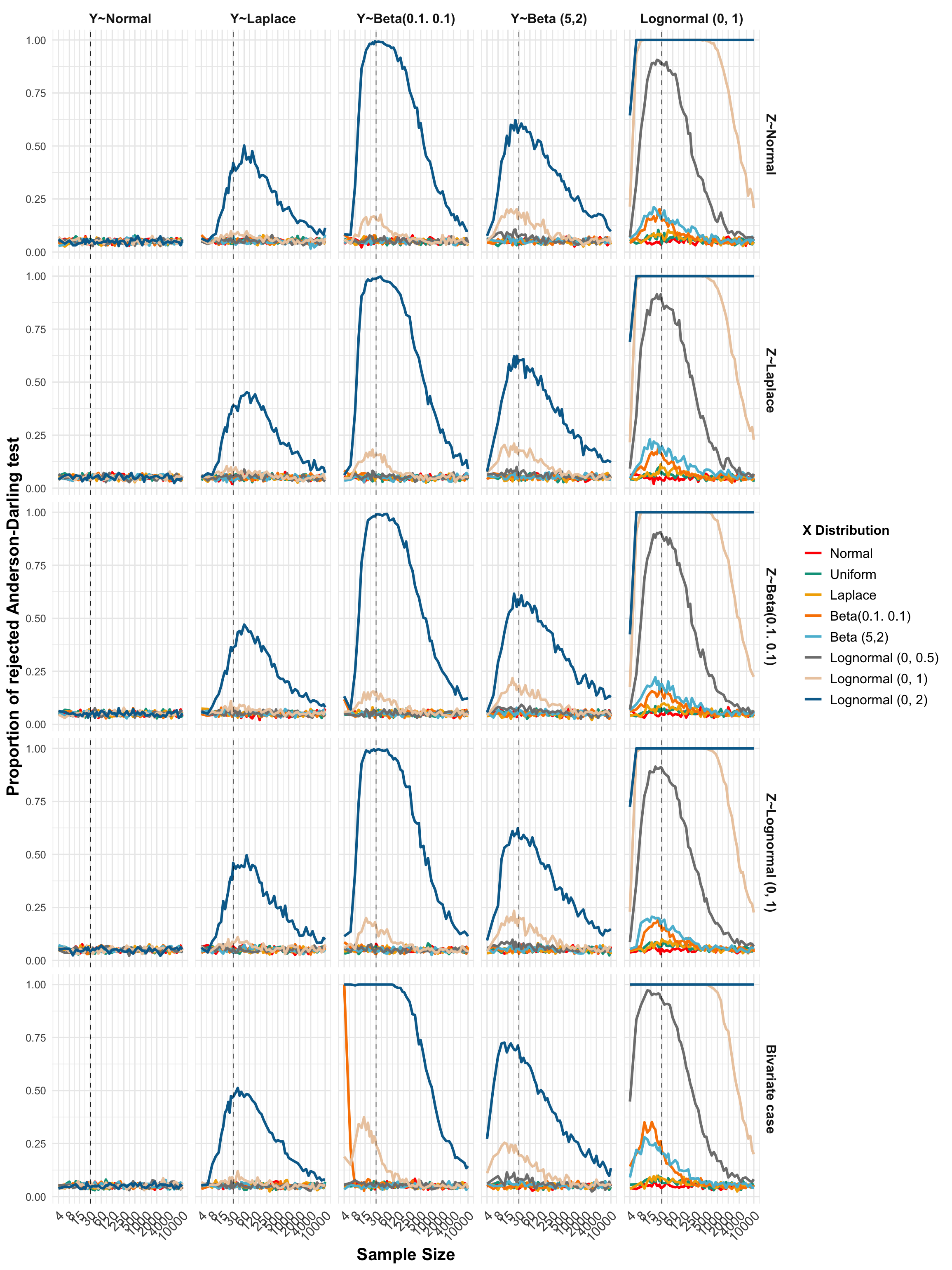
To test the distributional rules of thumb and provide additional guidance on the lower limit of for regression analysis, I set up a simple simulation study. In the simulation study, a dependent variable is first generated from a specific distribution. An independent variable is then generated from its own distribution. The variable is generated such that the theoretical mean is zero333This is done by subtracting the expected value of the distribution that is generated from and independent of . This means that in the simulation, the null hypothesis that is true. After this, a regression model are estimated and the t-values, i.e. , are extracted. The simulation procedure is repeated 1,000 times to produce a distribution of estimated t-values for each combination of and distributions of and .
Since the data are generated under the null hypothesis, the t-values extracted from the simulation should follow a t-distribution with degrees of freedom for our inferences to be valid. In other words, if the extracted t-values follow a t-distribution, we can be satisfied that we have a large-enough for the distributional assumptions of linear regression to be fulfilled.
To test if the resulting distribution of t-values actually follows a t-distribution, I use an Anderson-Darling distributional test on the resulting distribution and reject the null hypothesis that the distribution belongs to the specified t-distribution if the resulting p-value is lower than 0.05. I then repeat this procedure 500 times and calculate the proportion of simulations in which the Anderson-Darling test rejects the null-hypothesis that the distribution is actually a t-distribution. As robustness tests I also estimate the less restrictive Cramer von Mises and Kolmogorov-Smirnoff distributional tests.
To assess the severity of the violations, I also calculate the type I error rate at for each of the coefficients in the regression models across each simulation. Finally, I also assess the effects of adding a second independent variable, , to the regression model on the rate of convergence to the t-distribution for the t-values for by repeating the simulation with from different distributions.
In this note, I am particularly interested in how distributional characteristics such as skewness and kurtosis of both the dependent and independent variable(s) affect the rate of convergence to the t-distribution for the resulting t-values. Therefore, I choose to simulate and under a range of different lepto-, meso- and platykurtic symmetric distributions as well as a range of variously skewed distributions. I also try a large range of ranging from 4 to 10,000.444In total I test 54 unique values of . These are shown in Table 2 the appendix The tested distributions with their corresponding skewness and kurtoses can be found in Table 1 in the appendix. In total 6,534 different combinations of , distributions and distributions are tested. Each simulation uses 500 repeats of 1,000 regression models, for a total of approximately 3.3 billion simulated regression models. In the multivariate case including I test an additional 37,800 combinations resulting in a total of approximately 22.2 billion simulated regression models in the bi- and multivariate case.555The computations were conducted on the Dardel PDC using resources provided by the National Academic Infrastructure for Supercomputing in Sweden (NAISS), partially funded by the Swedish Research Council through grant agreement no. 2022-06725
5 Results
The results for a select few combinations of and distributions are shown in Figure 1 below.666Results for all combinations of distributions are available in the appendix, as are the results using the alternative distributional tests These results highlight some interesting patterns. First, it is not only when the residuals of the regression model are normal that regression modelling seems to perform well with a low number of observations . Rather, as long as both and are symmetric the distribution of the t-values converges to the t-distribution already at , except in the most extreme platykurtic case (Beta 0.1,0.1) where convergence is reached at . Similarly, if either or are symmetric and the other is skewed the distribution of t-values also converge to the t-distribution at unless the skewness of the other variable is severe (e.g. log-normal with ). This highlights that, contrary to theory, both the distribution of and matter for the convergence of the t-values to the t-distribution.

When both and are skewed, the rate of convergence seems to depend on both the skew of and of . In the most extreme cases, where both and follow log-normal distributions with parameter , the t-values do not converge to the t-distribution even at . Except when or are normal, the distribution of t-values do not converge to the t-distribution at when the other variable follows a log-normal distribution with .
5.1 Effects of non-convergence to the t-distribution
To assess the effects of the t-values not converging to the t-distribution I computed the type-I error rate across simulations. The results for a select few combinations of and distributions are shown in figure 2 below.777Results for all combinations of distributions are available in the online appendix.. As discussed earlier, the main concern about the t-values not converging to the t-distribution is that the p-values obtained from the regression analysis are no longer valid. This is especially problematic if the risk of type-I errors is higher than since we then risk rejecting null hypotheses when our evidence does not support this rejection.

The results from the simulation show that the consequences of the t-values not converging to the t-distribution depends on the skewness and kurtosis of the variables involved, and particularly the kurtosis. For the cases where the type-I error rate is not at the appropriate level and either of the variables are platykurtic, the type-I error rate is lower than , except when . If neither of the variables are platykurtic but are symmetric, the type-I error rate is higher than . The most extreme cases, where both and are log-normal with , exhibit a strange pattern where the type-I error rate is higher than alpha for low , but lower than for higher . The results also show that for some combinations of and distributions where the Anderson-Darling test has an appropriate rejection rate, the type-I error rate has not converged to (e.g. when or are normal and the other distribution is log-normal with ).
In general, however, the results also show that the effect of the t-values not converging to the t-distribution is not as severe as one might expect. For example, even in the worst case where both and are log-normal with , the type-I error rate is only approximately 0.06 when , i.e. only 0.01 higher than . While the effect is larger on the platykurtic distributions, the type-I error rate for these are lower than , which is less problematic than if the type-I error rates are higher than since this simply constitutes a more conservative test.
5.2 The multivariate case
To assess the effect of having a second independent variable in the regression model I also ran simulations where was added to the regression model. was generated under different distributions to assess whether the skewness and kurtosis of affected the convergence of the t-values associated with to the t-distribution. The results of this evaluation, presented in the appendix, shows that the distribution of did not have any substantial effect on the convergence of the t-values associated with regardless of the distribution of . This suggests that the distribution of additional independent variables, under the null hypothesis, does not affect the convergence of the t-values associated with to the t-distribution and thus that the results from the simulation in the bivariate case can be generalized to the multivariate case.
6 Discussion
This research note suggests that it is time to update what we teach our students with regards to the lower limit of the number of observations. Specifically, the assumption that the residuals follow a normal distribution or that the number of observations is sufficiently large can actually be relaxed to that the distribution of either of the variables involved is symmetric or that the number of observations is sufficiently large. This research note also shows that what is sufficiently large depends heavily on the distributional characteristics, especially the skew, of the variables involved.
Generally, the effect of the t-values not converging to the t-distribution is not as severe as one might expect, with the type-I error rate typically only being slightly higher, or lower, than in most cases. Overall, the results suggest that unless the variables are highly skewed, the rule of thumb seems to hold for most combinations of distributions and may even be considered conservative for some combinations of distributions.
What does this mean for researchers? The results suggest that it is possible to run regressions with fewer observations than previously thought, as long as the distribution of the variables involved are not too skewed. This means that in situations where researchers may have preferred to run less powerful non-parametric tests such as the Mann-Whitney U test due to few observations and non-normality, it may be possible to run a regression analysis instead if the variables are symmetric, or at least not too skewed even when the number of observations are low. At the other end of the spectrum, the results also suggest that the rule of thumb may be too permissive in some cases, such as when the variables are highly skewed.
The results also suggest that the kurtosis of the variables involved also affect what the effects of violations of the normality assumption are. In particular, if either of the distributions of the variables are platykurtic, the type-I error rate is lower than even when the t-values do not converge to the t-distribution. This is less problematic than if the type-I error rate is higher than since this simply constitutes a more conservative test.
A general recommendation from this paper is that researchers should report the skewness and kurtosis of the variables involved in the regression analysis, and that the researchers should reflect on the distributional characteristics of the variables when deciding on the number of observations needed. If either of the distributions of the variables are symmetric or platykurtic, fewer than 30 observations seem in general to be sufficient. Apart from these cases, the rule of thumb seem to hold for most combinations of distributions except when the distributions of either or both of the variables are highly skewed.
That it is possible to run regressions with fewer observations than previously thought does not mean that it is a good idea to do so. Power should still always be considered and the results from this research note should not be taken as a recommendation to run regressions with few observations. The results do, however, suggest that the distributional assumptions needed for us to be able to trust the t-values are not as strict as previously thought.
Further research should be directed at investigating the relationship between skewness and convergence to the t-distribution in order to develop guidlines for the lower bound of regression analysis, and to repeat this simulation study in a situation with more than one independent variable.
References
References
- Carsey, Thomas M, and Jeffrey J Harden. 2013. Monte Carlo Simulation and Resampling Methods for Social Science. Thousand Oaks, CA: SAGE Publications.
- Cohen, Jacob. 1992. “Things i Have Learned (so Far).” In Annual Convention of the American Psychological Association, 98th, Aug, 1990, Boston, MA, US; Presented at the Aforementioned Conference. American Psychological Association.
- Green, Samuel B. 1991. “How Many Subjects Does It Take to Do a Regression Analysis.” Multivariate Behavioral Research 26 (3): 499–510.
- Hesterberg, Tim. 2008. “It’s Time to Retire the Rule.” In Proceedings of the Joint Statistical Meetings.
- Hogg, Robert V, Elliot A Tanis, and Dale Zimmerman. 2013. Probability and Statistical Inference. 9th ed. Upper Saddle River, NJ: Pearson.
- Kwak, Sang Gyu, and Jong Hae Kim. 2017. “Central Limit Theorem: The Cornerstone of Modern Statistics.” Korean Journal of Anesthesiology 70 (2): 144.
- Thompson, Jeffrey Bear. 2023. “Approximating Infinity: An Investigation of the n= 30 Rule of Thumb.” Master's thesis. California State University, Long Beach.
- Wooldridge, Jeffrey. 2012. Introductory Econometrics: A Modern Approach. 5th ed. Mason, OH: CENGAGE Learning Custom Publishing.
Appendix A: Included distributions and n
Included distributions
| Distribution | Theoretical skew | Theoretical kurtosis |
|---|---|---|
| Normal | 0.00 | 3.00 |
| Uniform | 0.00 | 1.80 |
| Laplace | 0.00 | 6.00 |
| Beta(0.1. 0.1) | 0.00 | 1.12 |
| Beta (5,2) | 0.60 | 2.88 |
| Beta (5,1) | 1.18 | 4.20 |
| Beta (5,0.5) | 1.93 | 7.25 |
| Lognormal (0, 0.5) | 1.75 | 8.90 |
| Lognormal (0, 1) | 6.18 | 113.94 |
| Lognormal (0,1.5) | 33.47 | 10078.25 |
| Lognormal (0, 2) | 414.36 | 9220559.98 |
Included levels of n
| From | To | By | Number of n levels |
|---|---|---|---|
| 4 | 28 | 2 | 13 |
| 30 | 50 | 5 | 5 |
| 60 | 100 | 10 | 5 |
| 120 | 200 | 20 | 5 |
| 250 | 500 | 50 | 6 |
| 600 | 1000 | 100 | 5 |
| 1250 | 2000 | 250 | 4 |
| 2500 | 5000 | 500 | 6 |
| 6000 | 10000 | 1000 | 5 |
Appendix B: Full results
Convergence to t-distribution

Type I errors

Alternative distributional tests
Cramer-von Mises test

Kolmogorov-Smirnoff test

The multivariate case