Full error analysis of policy gradient learning algorithms for exploratory linear quadratic mean-field control problem in continuous time with common noise
Abstract
We consider reinforcement learning (RL) methods for finding optimal policies in linear quadratic (LQ) mean field control (MFC) problems over an infinite horizon in continuous time, with common noise and entropy regularization. We study policy gradient (PG) learning and first demonstrate convergence in a model-based setting by establishing a suitable gradient domination condition. Next, our main contribution is a comprehensive error analysis, where we prove the global linear convergence and sample complexity of the PG algorithm with two-point gradient estimates in a model-free setting with unknown parameters. In this setting, the parameterized optimal policies are learned from samples of the states and population distribution. Finally, we provide numerical evidence supporting the convergence of our implemented algorithms.
Key words: Mean-field control; reinforcement learning; linear-quadratic; two-point gradient estimation; Polyak-Lojasiewicz inequality; gradient descent; sample complexity.
1 Introduction
The last decade has seen significant advances in solving optimal control of dynamical systems in unknown environments using reinforcement learning (RL) methods. The essence of RL is to learn optimal decisions through trial and error, which involves repeatedly trying a policy, observing the state, receiving and evaluating the reward, and subsequently improving the policy. There are two main approaches in RL: (i) -learning, which is based on dynamic programming, and (ii) policy gradient (PG), which is based on the parametrization of policies. A key feature of RL is the exploration of the unknown environment to broaden the search space, achievable through randomized policies. RL is a very active branch of machine learning. For an overview of this field in the discrete-time setting, we refer to the second edition of the monograph [20], and for recent advances in the continuous-time setting, see [14] and [15].
Mean-field control (MFC), also known as the McKean-Vlasov (MKV) control problem, is a class of stochastic control problems that focuses on the study of large population models of interacting agents who cooperate and act for collective welfare according to a central decision-maker (or social planner). This field has attracted growing interest over the last decade, resulting in a substantial body of literature on both its theory and its various applications in economics, finance, population dynamics, social sciences, and herd behavior. For a detailed treatment of the topic, we refer to the seminal two-volume monograph [4, 5].
RL for MFC has recently attracted attention in the research community, see e.g. [6], [11], [1], [9], [19]. The challenge lies in accurately learning optimal policies and value functions defined on the infinite-dimensional space of probability measures. The mathematical understanding and convergence analysis of these RL algorithms are still in their infancy.
In this paper, we aim to address questions surrounding convergence and sample complexity, focusing on policy gradient methods in RL within the context of infinite horizon linear quadratic (LQ) MFC with common noise for continuous time systems. The LQ problem is indeed the cornerstone of optimal control theory due to its tractability and can be viewed as an approximation of more general nonlinear control problems. To encourage exploration in unknown environments, we employ randomized policies and add entropy regularization, following the approach of recent papers [14], [12], [22], [10], [21].
Our main contributions.
Our paper proposes and analyzes convergent PG algorithms to solve infinite horizon exploratory LQ MFC problems in a continuous time setting, with common noise and entropy regularization.
-
•
Our first contribution is to derive the explicit form of the optimal solution using coupled algebraic Riccati equations, thereby generalizing the results in [2] to include entropy regularization for randomized policies (Theorem A.1). Motivated by the explicit form of the optimal randomized policy, we reformulate the LQ MFC problem into a minimization problem over Gaussian policies. The mean of each Gaussian policy being linear in the state and conditional mean with respect to the common noise is parameterised using two matrix-valued coefficients . The parameterized cost function is shown to be smooth and satisfy a gradient domination condition, also known as the Polyak-Lojasiewicz inequality (Propositions 3.1 and 3.2) following the approach of [8] and [23]. Such inequality is known to be crucial to ensure the convergence of PG algorithms in non-convex landscape.
-
•
We then propose and study PG methods in both exact and model-free settings. Our work provides theoretical guarantees of convergence for the gradient descent (GD) algorithms with suitable step sizes (Theorems 3.1 and 4.1). In the model-free case, where the exact gradient is unavailable, we adapt the two-point gradient estimation method of [16] to our mean-field setting by relying on samples of discrete-time trajectories and population distributions. For the first time to the best of our knowledge, we provide a comprehensive error analysis accounting respectively for the error of perturbation with respect to the exact expected functional cost, for the horizon truncation, for the time and particle discretizations, for the statistical error and finally for the optimization error from gradient iterations, demonstrating global linear convergence with polynomial computational sample complexities.
Related works.
The closest papers related to our work are [6] and [23]. In [6], the authors consider an LQ MFC problem with common noise in a discrete time setting and prove the convergence of PG algorithms for deterministic policies in both model-based and model-free settings. The paper [23] addresses an infinite-horizon time average LQ MFC control problem in a continuous time setting without an entropy regularizer and demonstrates the convergence of PG with deterministic policies in the exact model-based setting, using a varying step size at each iteration. Finally, it is worth mentioning that our proofs extend the arguments presented in [8] and [13] for the discrete time setting, covering both finite and infinite horizons, as well as those in [16] and [3] for the continuous time setting. In these references, the authors demonstrated convergence results for standard LQ problems.
Outline.
The paper is organized as follows. In Section 2, we formulate the exploratory LQ MFC problem in continuous time with common noise, provide the theoretical optimal policy, and discuss parameterization in the model-free case. In Section 3, we demonstrate the convergence of the model-based gradient descent algorithm using the gradient domination condition. Section 4 presents the gradient estimation algorithm employing the population simulator and develops the convergence analysis of the model-free gradient descent algorithm. In Section 5, we provide numerical experiments that illustrate our convergence results for both the model-based and model-free algorithms. The proofs of all results are included in the Appendix.
Notations.
-
•
We denote by the scalar product between the two vectors , , and by the inner product of the two matrices with compatible dimensions, where is the transpose matrix of . The Frobenius norm of a matrix is defined by .
-
•
is the set of symmetric matrices, and (resp. is the set of nonnegative (resp. positive definite) matrices in . The partial order on is defined as: if . We also write to mean that .
2 Problem formulation
2.1 Setup and preliminaries
The linear dynamics of the mean-field state equation with randomized controls and common noise is described by
| (2.1) |
on a probability space supporting two independent Brownian motions (the idiosyncratic noise), and (the common noise), of dimension and . For convenience, we choose the probability space in the product form , and denote by the right-continuous completion of the canonical filtration generated by , and by the right-continuous completion of the canonical filtration generated by . The initial condition is an -random variable, which is -measurable, where is a -algebra independent of . We denote by .
Here, stands for the conditional expectation given , , are constant matrices in , is a constant matrix in , is a constant matrix in , is a constant matrix in , and in the sequel, we shall denote by .
The randomized control is an -progressively measurable process in , the set of probability measures on the action space with a finite second order moment. We shall consider randomized controls with densities , .
The infinite horizon LQ MFC problem consists in minimizing over such randomized controls the quadratic cost functional with entropy regularizer of parameter :
| (2.2) | ||||
| (2.3) |
Here , are constant matrices in such that , and . Notice that the cost functional is written equivalently as
| (2.4) | ||||
| (2.5) |
Assumption 2.1.
The two following Algebraic Riccati Equations (ARE) for and respectively admit a unique positive definite solutions:
| (2.6) | ||||
| (2.7) |
Remark 2.1.
Under Assumption 2.1, the optimal randomized control, solution to (2.4) is given in feedback policy form as , where is the normal distribution
| (2.8) |
and where is the state process with randomized control and is the unique positive definite solution to (2.6)-(2.7). Moreover, the optimal cost is given by
| (2.9) |
where
| (2.10) | ||||
Here, denotes the covariance matrix of . In Appendix A, we state and prove this result in a more general case.
Throughout the remainder of this paper, we shall also assume that the following assumption is in force.
Assumption 2.2.
belongs to , i.e. where denotes the smallest eigenvalue of a square matrix.
Remark 2.2.
The above assumption for is satisfied when . As for , denoting by , the augmented matrix formed by and , we have . Thus, if and only if is of rank , which requires that that .
2.2 Model free perspective and reparametrization
In this section, we are interested in the model-free setting for the linear mean-field dynamics of state process, i.e., when the parameters in (2.1) are unknown, and so the optimal policy in (2.8) cannot be implemented from the unique solution to the Riccati system (2.6)-(2.7).
Motivated by the Gaussian distribution of the optimal randomized policy, whose mean is a linear combination of and , we propose the following parameterization of the randomized policy:
| (2.11) |
where are the two-parameter matrices to be optimized. The density of the parametrized randomized policy is explicitly given by
The associated dynamics of the parametrized process , starting from , is given by
| (2.12) |
where , with density . The corresponding cost function, now defined as a function on , is expressed (with a slight abuse of notation) as follows:
| (2.13) | ||||
| (2.14) |
where , with the objective of minimizing the parameterized cost function over . It is clear from (2.8) that , and the solution to this minimization problem is given by
| (2.15) |
where is the solution to the ARE (2.6) and (2.7), ensuring that .
Let us introduce the parametrized auxiliary processes
| (2.16) |
By observing from the definition of that
| (2.17) |
we see from (2.12) that the dynamics of is decoupled and governed by
| (2.18) |
with and . Notice that (resp. ) depends on only via the first (resp. second) component parameter (resp. ), and we shall then write , .
Moreover, by noting that
| (2.19) | ||||
| (2.20) |
the parametrized cost in (2.14) can be written as a quadratic function of , namely:
| (2.21) |
recalling that is given by (2.10). An important observation is that it can be decomposed as follows
| (2.22) |
where
| (2.23) |
with
| (2.24) |
so that the minimization over amounts to separate minimization problems:
| (2.25) |
In fact, we now demonstrate that the two aforementioned minimization problems over and can be reduced to suitable smaller sets defined by
| (2.26) |
recalling that , on which the problem is well-posed.
Lemma 2.1.
The minimizers in (2.15) satisfy , , and thus
| (2.27) |
Proof.
The ARE (2.6) for rewrites as
| (2.28) |
Since then , hence all the eigenvalues of the matrix on the r.h.s. of (2.28) are strictly negative. Moreover, since , if the matrix has a non-negative real part eigenvalue, then the largest eigenvalue of the matrix on the l.h.s. of (2.28) is non-negative and therefore cannot be equal to the matrix on the r.h.s. It follows that is stable, which means tht .
Similarly, by using the ARE (2.7) for , we show that is also stable, i.e., ∎
We now state a characterization of the two matrices and defined in (2.24).
Proposition 2.1.
For all , the matrices and are well-defined in and are the unique positive definite solution to the following Algebraic Lyapunov Equations (ALE):
| (2.29) | ||||
Proof.
Cf Appendix B.1 ∎
We conclude this section by providing an alternate useful expression of the cost functions and defined by (2.23) on which the minimization over and will be performed.
Proposition 2.2.
For all , we have
| (2.30) |
where and are the unique elements in solutions to the ALE
| (2.31) | ||||
| (2.32) |
Proof.
Cf Appendix B.2 ∎
Remark 2.3.
Note that, according to (2.9), we have and .
3 Model-based PG algorithm
In this section, we establish the convergence of the gradient descent algorithm towards the optimal parameters assuming full knowledge of the model parameters, thus allowing for the exact computation of the gradient. This foundation will facilitate the learning of optimal parameters in the model-free setting in the subsequent section, despite the nonconvex optimization framework. Furthermore, the gradient descent method in the model-based scenario offers an alternative to solving the Riccati system (2.6)-(2.7), which is computationally intensive, while the convergence result (Theorem 3.1) remains dimension-free.
Given , the updating rule at step for the exact gradient descent of the minimization problem (2.25) is given by
| (3.1) |
where is the constant step size (learning rate), and and are the gradients of and with respect to their respective parameters.
3.1 Gradient domination condition
We first provide an explicit formula for the gradient that will be used for the implementation of the (exact) gradient descent rule.
Proposition 3.1 (Expression of the gradients).
For , it holds
| (3.2) |
where and .
Proof.
Cf. Appendix C.1 ∎
Next, to assess the convergence of the aforementioned gradient descent algorithm in this nonconvex landscape, we will demonstrate that the cost functions and satisfy a Polyak-Lojasiewicz (PL) inequality on and , respectively, also known as the gradient domination condition.
Proposition 3.2 (Gradient domination).
There exist two positive constants such that for any ,
| (3.3) |
More precisely, the constants and are given by
| (3.4) |
Proof.
Cf. Appendix C.2 ∎
3.2 Global convergence of model-based PG algorithm
For fixed , we define the level subsets of and as follows:
| (3.5) |
In the sequel, we shall naturally restrict to and to avoid empty level sets.
We now show that both gradient maps and are Lipschitz-continuous on and respectively.
Proposition 3.3.
There exist explicit positive constants
| (3.6) | ||||
| (3.7) |
such that is -Lipschitz continuous on and is -Lipschitz continuous on , that is, for all and all
| (3.8) |
Proof.
Cf. Appendix C.3 ∎
The following theorem is the main result of this section and states the linear convergence rate of the gradient descent method. A key point is to prove that the sequence always lies in provided that one starts from an initial point with a suitably chosen common step size .
Theorem 3.1 (Global convergence of the exact gradient descent method).
Let and select a constant step size where
| (3.9) |
Then, the sequence generated by the exact GD algorithm (3.1) stays in . Moreover, for any fixed accuracy , we achieve
| (3.10) |
with a number of iterations satisfying
| (3.11) |
where
| (3.12) |
Remark 3.1.
In the model-based case, since we can compute and explicitly, one can choose and for any .
The proof of the above convergence result is based on the following stability result which shows that both and are stable by the one step transition of the GD algorithm.
Lemma 3.1.
If and , then for all , it holds
| (3.13) |
Proof.
For a fixed , we let
| (3.14) |
From the first order Taylor expansion and the continuity of , one has
Since , we have and then for all small enough, we have which implies that and thus . Moreover, from Proposition C.1 where it is shown that is bounded, we deduce that .
The definition of implies that for any and any , since .
Now the second-order Taylor’s expansion for combined with the local Lipschitz continuity of stated in Proposition 3.3 guarantees that
| (3.15) |
Suppose that . From the continuity of , and the definition of , we have . Then, by (3.15), we get
| (3.16) |
which implies (as ) that
| (3.17) |
This contradicts the fact that . Therefore, we conclude that and for all , . Similar arguments show the result for . In particular, one shows that for all , . In conclusion, for all , it holds at the same time
| (3.18) |
∎
Proof of Theorem 3.1. Start from some fixed stabilizing initial parameter . Since , by choosing a step size , Lemma 3.1 guarantees that
| (3.19) |
Moreover, by (3.16), the following inequalities hold
| (3.20) |
The definition of together with the gradient domination condition of Proposition 3.2, ensures that for all ,
| (3.21) |
and that for all
| (3.22) |
Hence, coming back to (3.20), we deduce
| (3.23) | |||
| (3.24) |
Summing the two previous inequalities, we obtain
By a direct induction argument, at each step , it holds
| (3.25) |
so that
| (3.26) |
We thus conclude
| (3.27) |
The above inequality readily leads to the rest of the assertions in the theorem.
Remark 3.2.
The problem of the solvability of the Lyapunov equations (2.31)-(2.32) have been investigated in [23]. The main difference with our result is that the authors in [23] have shown that if and with the perturbation depending on then . Therefore, at each step , they choose the step size according to in order to make the perturbation less than .
Here, we adopt a different approach: we truncate and define a compact subset . We demonstrate that is Lipschitz continuous on with a Lipschitz constant and directly choose the step size according to , ensuring that the sequence remains in . Thus, remains constant throughout all iterations. We refer to [16] for a detailed description of the method we have extended to solve an LQ MFC problem. It is important to note that in [16], the only source of randomness is the initial value.
4 Model-free PG algorithm
4.1 Notations
In the model-free setting, we do not have access to the values of the functions and , or their gradients, as the model coefficients are unknown. Hence, we combine the two parameters . The value function is then regarded as a function defined on .
For all , we define the norm of by
| (4.1) |
and for , their inner product is defined by
| (4.2) |
We let
| (4.3) |
and, for , we define the level subset of by
| (4.4) |
where
| (4.5) |
Note that is obtained by removing the constant part that depends only on from .
Since and are non-negative functions, one has . Having shown that both and are compact subsets of , we get that is bounded. The continuity of on also implies that is closed. Since is of finite dimension, we deduce that is compact.
Finally, one can define the total gradient of and as
| (4.6) |
According to Theorem 3.2, the gradient domination inequality holds:
| (4.7) |
where . The same inequality also holds for .
4.2 Model-free PG algorithm with population simulator
In the current model-free setting, we do not explicitly know the gradient . Therefore, the GD algorithm from the previous section cannot be directly applied. Instead, we rely on a stochastic PG algorithm based on a stochastic population simulator, which provides an approximation of the controlled MKV dynamics (2.12) along with the associated cost (2.14).
For a finite terminal horizon and a positive integer , we consider the uniform time grid of the interval given by where , , and . For a given positive integer , the interacting agents system with states evolves according to the dynamics
| (4.8) | ||||
where , , and the action that the -th agent takes at time is drawn as independently of . Here, are -dimensional Brownian motions on and is the common noise on , and is independent of .
In the spirit of [21], the population simulator samples the randomized actions as follows
| (4.9) | ||||
where the action simulation noises are i.i.d. random variables independent of with law . In particular, one may assume that is rich enough to support not only but also the sequence .
Introducing the notations , the dynamics (4.8) writes
| (4.10) | ||||
and we notice that are exchangeable in law.
The discounted running cost at time of the -th agent is defined by
| (4.11) | ||||
and the average cost estimation of the population over the interval for a given is given by
| (4.12) | ||||
Note that, since , , and the density are known, the last term in the above expression can be computed explicitly.
In the spirit of [8], see also [7] and [6], we compute in Algorithm 1 a biased estimator of the true gradient
based solely on the average cost estimation (4.12).
We let be the ball of radius (with respect to the Frobenius norm) centered at the origin, and be its boundary. The uniform distribution on is denoted by .
-
•
Sample and i.i.d.
-
•
Define perturbed feedback parameters
-
•
Sample via the population simulator (4.12) for .
We are now in position to define our (stochastic) model-free PG algorithm. Given , for some , recalling (4.4), we update the parameters as follows
| (4.13) |
for some well-chosen constant positive learning rate .
Our main contribution is the following convergence result of the model-free PG sequence as given by (4.13).
Theorem 4.1.
Let be a prescribed accuracy and be the constant learning rate. Then, choosing small enough such that
recalling that is the coefficient in the gradient domination condition appearing in (4.7), choosing large enough such that
choosing the number of periods in the grid large enough such that
taking the number of particles large enough such that
and finally taking the number of samples in Algorithm 1 large enough such that
it holds
with probability at least in at most
iterations.
The proof is deferred to Section D of the appendix. In the above convergence result, , , , , , , , and are explicit functions whose definition is provided in the proof. In particular, is defined in Lemma D.1, are defined in Propositions D.2, D.5, , are defined in Proposition D.3, is defined in Proposition D.4, is defined in Proposition D.6 and are defined in Propositions D.2, D.5.
Remark 4.1.
Regarding the choice of , we recall the definition of the level set, in (4.4)-(4.5)- and is the superior limit of , where is the expected function cost in which we removed the known constant (since are known). Hence, a natural choice is to take and one can replace by its sample average approximation using the average cost estimation of the population (4.12).
5 Numerical example
We demonstrate the convergence analysis of our algorithms using a one-dimensional example with the following model parameters:
The optimal parameters (2.15) are . Thus, the optimal cost is given by , . Both model-based and model-free algorithms are initialized with .
5.1 Model-based algorithm
In the model-based case, we can derive explicit formulas for and , along with their derivatives and , using the results obtained in Sections 2 and 3.
We evaluate the PG algorithm (Algorithm 3.1) using three different step sizes: . Figure 1 illustrates the convergence of the sequence towards in terms of the number of iterations.


Then, Figure 2 illustrates the convergence of the cost functions and by plotting the relative errors and .


The PG algorithm 3.1 demonstrates very good performance. The error and the error rate of the value function converge to zero after roughly 200 iterations for different values of the learning rate.
5.2 Model-free algorithm
We use the following parameter values for the model-free PG algorithm:
The optimal cost corresponding to the parameters given in Table 1 is . First, we test whether the parameters in Table 2 allow for accurate gradient estimations. In Figure 3, we evaluate this for , by generating 100 gradient estimations using the gradient estimation algorithm (Algorithm 1).
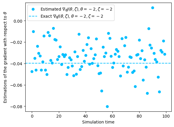

In the figures above, the vertical coordinates of the points represent the estimated gradients, with the dashed line indicating the exact gradients. We observe that most points cluster around the dashed line, remaining within above and below it. This suggests that, with high probability, the error in gradient estimation is controlled within , indicating that the parameters in Table 2 are well-chosen.
Our main result (Theorem 4.1) is established for a constant step size . However, from a numerical standpoint, one might consider exploring adaptive selection of by adjusting it based on the observed behavior of the cost function . Specifically, if is in an acceptable interval (an open interval), the cost function should decrease. According to the findings of the model-based algorithm, increasing (while ensuring it remains within the acceptable interval) may accelerate convergence.
Therefore, we can initialize with a and run the algorithm for several iterations (e.g., 100) initially. If we observe a clear downward trend in the (estimated) cost function , it indicates that our chosen falls within the acceptable interval. We can then consider increasing slightly to potentially accelerate convergence. Conversely, if we do not observe a decreasing trend, we should consider reducing .
The above results are based on the following choice of the step size as a function of the iteration index :
In Figure 4, we observe the convergence of both sequences and towards and respectively.


In Figure 5, we plot the error (on the left side) and the error rate (on the right side) as a function of the number of iterations. As in the model-based case, we observe excellent performance of the policy gradient algorithm. Both the error and the error rate on the value function vanish after approximately iterations.


Appendix A Explicit solution to LQ MFC
Let us consider the more general linear mean-field dynamics
| (A.1) |
and a quadratic cost with entropy regularizer
| (A.2) | ||||
| (A.3) |
to be minimized over randomized controls with density of feedback form: for some randomized policy . For simplicity of presentation, we assume here that and are one-dimensional Brownian motions, see Remark A.2 for the extension to the multi-dimensional case.
Theorem A.1.
Assume that the two following coupled Riccati equations for and have a unique positive definite solutions
| (A.4) |
Let be the unique positive definite solutions to (A.4) and be the solution to
| (A.5) |
Then the optimal randomised control is of feedback form with Gaussian distribution, namely for all , with
where is the unique solution to (A.1) with . Moreover, the optimal functional cost satisfies
Proof.
We employ the same Martingale approach as in [9] and [2] to prove that is the optimal policy, noting that the value function is time-independent in the infinite horizon case. In what follows, we omit the dependence of the process w.r.t the control.
Step 1. Let us consider the function defined on by , recalling that stands for the mean of , where is defined by
| (A.6) |
for some matrices/vectors , and . Then, given with density and the unique solution to (A.1), we introduce the following process
where we set the density function of for . Note that satisfies
Step 2. The derivatives of are given by
Moreover, using the dynamics of and , we obtain
Applying Ito’s rule to , we obtain
| (A.7) | ||||
and taking conditional expectation on both sides of the preceding equality
| (A.8) | ||||
Step 3. Referring to Lemma 6.3 in [2], we try to show that is non-decreasing for all and is constant for . Applying Ito’s formula to and taking expectation we get
| (A.9) |
with
Then, using (A.7) and (A.8), we obtain
| (A.10) | ||||
so that
| (A.11) | ||||
Step 4. We introduce the map
| (A.12) |
Following the approach outlined in Step 3 of the proof of Theorem B.1 in [9], the optimal policy that minimizes is given by:
and the infimum writes
| (A.13) | ||||
Step 5. Noting that is strictly positive-definite, for all , we have
| (A.14) | ||||
Now, taking as the solutions to (A.4)-(A.5) and letting
we observe that the right hand side of (A.14) vanishes, which means that for all , . Moreover, equality in (A.14) holds true for so that
| (A.15) |
We thus conclude that for any , is non-decreasing on and is constant on which eventually implies
| (A.16) |
The proof is now complete. ∎
Remark A.1.
Appendix B Proof of Propositions 2.1 and 2.2
B.1 Proof of Proposition 2.1
We first provide two auxiliary technical results.
Lemma B.1.
(Solution to the ODE for symmetric matrix-valued function)
Let be the solution the following ODE
| (B.1) |
for some and . Then, it holds
where .
Lemma B.2.
If , then it holds
| (B.2) |
Proof.
From the dynamics (2.18) of and Itô’s rule for and , we get
| (B.3) | ||||
so that
Now, if , then both and are stable which allows to conclude. ∎
Proof of Proposition 2.1: Using the integration by parts, we have
Using (B.3) together with the previous identity, we get
so that defined by (2.24) satisfies
which in turn, recalling that , allows to conclude. The proof for is similar. We thus omit the remaining technical details.
Expressing (2.29) in the standard form of the Lyapounov equation
and, recalling that , we conclude that they admit a unique positive definite solution.
B.2 Proof of the Proposition 2.2
Since , the above equations admit a unique positive definite solutions.
Appendix C Proofs of results for model-based algorithms
C.1 Proof of Proposition 3.1
We prove Proposition 3.1 only for , as the part concerning follows similar reasoning. First, we recall an auxiliary result regarding the exponential form of the solution to continuous Lyapunov equations.
Lemma C.1.
(Solution of continuous Lyapunov equation). Let be a stable matrix and a symmetric matrix. The following continuous Lyapunov equation
admits a unique solution which satisfies
Hence, recalling the algebraic Riccati equation (2.32) for , we deduce that
In order to differentiate , we will rely on the following definition of the derivatives of a matrix-valued map.
Definition C.1.
(Differentiability of the matrix applications)The map is differentiable at if there exists a matrix mapping: such that for any
where ’vec’ stands for the vectorization operator defined for by
Lemma C.2.
(Diffentiability of with respect to ) Denoting , for all , , we have
from which it readily follows that there exists a matrix depending only on such that
Proof.
Taking the difference between the two equations (2.31) solved by and , we get
so that is the unique solution to the following Algebraic Lyapounov equation for
From Lemma C.1, we thus obtain
The previous identity directly gives
where
Note that in the last line we again used the expression of . Thus, there exists that depends on and such that
We conclude that is indeed differentiable with respect to . ∎
We recall the rules of the total differentiation of the matrices:
-
(1)
-
(2)
-
(3)
-
(4)
We are now in position to prove Proposition 3.1. We only prove the identity for the gradient of , as the gradient of can be treated similarly.
By the definition of the differentiation
Since , we have so that
Then, we differentiate totally the Lyapunov equation of and obtain
which writes
We then multiply from the right the above equation by . We obtain
Using the fact that satisfies the equation
we get
where in the second and the fourth lines we used the commutative property of the trace operator. Comparing the left and the right sides of the previous identity, we eventually get
The proof of Proposition 3.1 is now complete.
C.2 Proof of Theorem 3.2
We here prove the Polyak-Lojasiewocz inequality stated in Theorem 3.2. We will only prove it for , as can be treated in a completely similar manner. We first need the following auxiliary result.
Lemma C.3.
(Perturbation analysis of ) For all , it holds
Proof.
We have
where for the last equality we used the algebraic Riccati equation of . ∎
C.3 Proof of Proposition 3.3
Let us recall that and are given by
with and where are the unique solutions to
and are the unique solutions to
Here again, we will only prove the Lipschitz continuity of , as can be treated in a similar manner.
C.3.1 Auxiliary results
We start by proving some useful bounds on when , and similar bounds for when ,
Proposition C.1.
For all , it holds
Similarly, for all , it holds
Before proving the above proposition, we will need the following technical result.
Lemma C.4.
For all , the following lower bound holds
Proof.
Proof of Proposition C.1
Step 1 (Bound for ). Recalling that , we directly deduce
so that
Step 2 (Bound for ). We use the fact that to deduce
which in turn implies
Step 3 (Bound for ). From Lemma C.4, we get
Step 4 (Bound for ). We first write
New operators. Taking a given stable matrix and a symmetric matrix , we define the two operators and by
| (C.1) |
It is known that
which means that .
Lemma C.5.
For all , it holds
Proof.
For any unit vector and any unit spectral norm matrix , it holds
which clearly yields the conclusion. ∎
Lemma C.6.
It holds
Proof.
From the commutative property of the trace operator, for any unit vector and any unit spectral norm matrix , one has
which yields
Noting that , the reverse inequality directly follows. ∎
In what follows, we introduce the notations
C.3.2 Lipschitz regularity of , , and .
Perturbation analysis for and
Hence, from Lemma C.5, we directly get
| (C.2) |
Proposition C.2.
For all , it holds
where . Similarly, for all , it holds
where .
Proof.
From
we get
Since we have
The Lipschitz regularity of is handled by similar arguments. The remaining technical details are omitted. ∎
Perturbation analysis of and .
Proposition C.3.
For all , one has
where
Similarly, one can show that for all , it holds
where
Proof.
From Lemma C.2, we get
so that
The compactness of together with the continuity of yields . The triangle inequality together with Proposition C.1 gives
so that
Gathering the previous bounds allows to conclude that is -Lipschitz continuous on . Similar arguments yield the Lipschitz regularity of . We omit the remaining technical details.
∎
C.3.3 Proof of Proposition 3.3
In order to establish the Lipschitz regularity of and on , we start from the representation provided by Proposition 3.1. Namely, one has
where . Hence,
The previous bound, along again with Proposition C.3, provides
Using similar arguments, we find that for all ,
where
Appendix D Proofs of the results for the model-free algorithm
In the first subsection, we describe the strategy of the proof of Theorem 4.1. In Subsection D.2, we provide its proof. Several auxiliary results are postponed to the next subsections.
D.1 Strategy of proof of Theorem 4.1
We first solve the well-posedness problem of the perturbation of the parameters. The following lemma is directly taken from Lemma 4 of [16].
Lemma D.1.
There exists depending only upon , , and the model parameters such that for all , for any such that and for all , we have
| (D.1) |
From now on, we assume that is small enough (, defined in Lemma D.1), so that for all , for all with .
The main ingredients of the proof can be described as follows. Denoting by where and are the results of Algorithm 1, the key idea is to show that the two following events
| (D.2) | ||||
occur together with high probability, for some . More precisely, by writing
and
we notice that if the event
| (D.3) |
occurs with high probability, then so does with and .
Next, for any fixed , the P.-L. inequality (4.7) guarantees that if is such that , then (D.3) is satisfied as soon as
with . Indeed, it suffices to notice that
Noting that
we will show that for all , the event
holds with high probability as soon as the parameters are large enough and is small enough.
D.2 Proof of Theorem 4.1
Step 1: The central idea is to use the following decomposition
and similarly
where we introduced the following notations which will be useful for our convergence analysis:
The perturbed policy gradients:
The truncated policy gradients:
The policy gradients with time discretization:
The output of Algorithm 1 averaged over the randomness of the state trajectories:
| (D.4) | ||||
where and .
In the above notations, given a finite horizon (to be chosen later on) and , we introduced the following time-truncated expected cost functional
| (D.5) | ||||
and also introduced the corresponding time discretized cost functional, with action execution noise
| (D.6) | ||||
where is the time-discretization scheme of , over the same time grid as the interacting agents dynamics (4.8), with dynamics
| (D.7) |
with , being i.i.d. random variables with law .
Step 2: Denoting by , choosing and , Proposition D.2 guarantees that with probability
Choosing large enough (again as in the statement of Theorem 4.1), according to estimates (D.13) in Proposition D.6, it holds
Finally, according to Proposition D.5, up to a modification of , namely taking large enough such that
one has
with probability .
Putting the above estimates together yields
so that
with probability at least .
Step 3: As discussed in Subsection D.1, the previous inequality implies that the probability of defined in (D.2) with and is not smaller than .
It then follows from Lemma D.1 that for any , still with the probability not smaller than , one has
and
By induction, we eventually deduce that
with probability at least . The conclusion of Theorem 4.1 easily follows from the previous inequality.
D.3 Analysis of the single step GD algorithm
In this section, we analyze the convergence of a general single-step GD algorithm. This part serves as an important building block in the proof of Theorem 4.1. Our main result is Proposition D.1. We first prove some technical results.
Lemma D.2.
Proof.
It is clear that implies so that
which in turn clearly yields
The proof is now complete. ∎
For and satisfying
| (D.8) |
we set
| (D.9) |
Proof.
We let
Firstly, from the first condition of , is also a descent direction of the function , we have . Next, is compact thus bounded, we have .
Assume that . By the continuity of and the definition of , we have . Therefore, for any , we have . A second order Taylor’s expansion together with the Lipschitz continuity of and (D.8) gives
so that
which in turn clearly gives
This last inequality contradicts the fact that . We thus conclude that and for all . ∎
D.4 Error analysis of and its gradient
We here study the five terms appearing in the decomposition of the error of and introduced in Step 1 of Section D.2.
Bounding (Error of perturbation with the exact expected functional cost).
The proof of the following result is postponed to Section D.4.1.
Proposition D.2.
For all , there exist with at most polynomial growth in and and with at most polynomial growth in , and such that for all , all and all ,
| (D.10) |
with probability at least .
Bounding (Horizon truncation error).
The proof of the following result is postponed to Section D.4.2.
Proposition D.3.
a.s., for all , one has
Bounding (Time discretization error).
The proof of the following result is postponed to Section D.4.3.
Proposition D.4.
There exists a constant (non-decreasing with respect to ) such that a.s., for all , it holds
Bounding (Statistical error).
The proof of the following result is postponed to Section D.4.4.
Proposition D.5.
(Statistical error on gradient estimators) For all , there exist and with at most polynomial growth in , , , , , such that for all and all , with probability at least , for all , it holds
| (D.11) | ||||
Bounding (Particle discretization error).
The proof of the following result is postponed to Section D.4.5.
Proposition D.6.
Let , , recalling that is defined by (4.12). There exists such that for all ,
| (D.12) |
Moreover, a.s., for all , it holds
| (D.13) | ||||
D.4.1 Proof of Proposition D.2
The proof is reminiscent of Lemma 31 [6] or Lemma 30 [8]. For any and , let us introduce the following smooth approximation of defined by
| (D.14) |
where and are two independent random variables uniformly distributed in and stands for the expectation taken with respect to the random variables .
The following result is directly taken from Lemma 26 in [8]. For any , it holds
| (D.15) | |||
We then write
| (D.16) |
For the second term , using the Lipschitz property of the gradient shown in the Section C.3, there exists with polynomial growth in and such that for all , for all and such that and , we have . Then according to (D.14), noticing that , we have
Then, for the first term , using (D.15), we notice that is exactly the Monte-Carlo approximation for the expectation . Assuming that , according to Lemma D.1, for all and each individual sample has the norm bounded by according to (4.4)-(4.5). Thus we can apply vector Bernstein’s Inequality to deduce that there exists with polynomial growth in , and such that for all , for all , we have with probability at least .
The bound for is derived in a similar manner, and thus its proof is omitted.
D.4.2 Proof of Proposition D.3
In order to establish our result on and , we first need to derive an error bound on .
Lemma D.4.
There exist two positive constants and depending only upon , the model parameters and such that for all
Besides, and are non-decreasing functions.
Before proving the above lemma, we will need the following technical result which is directly taken from Lemma 12 [16]. Its proof is thus omitted.
Lemma D.5.
Let the matrices and satisfy
then for any ,
where denotes the largest singular value of the matrices.
In particular, note that defined in (2.10) is in fact for .
Denoting for simplicity and , one has
| (D.18) |
As proved in Lemma B.2 (using Itô’s formula),
so that
Hence,
and similarly
Since , recalling that as well as are compact sets, using the continuity to and , there exist such that for all
and using the fact that , we get
and
By using again the fact that is compact, there exists a constant such that for all :
Combing back to (D.18) and plugging the above estimates, we obtain for all
for some and depending only upon and .
Finally, the monotonicity of and with respect to is a consequence of the fact that if then .
D.4.3 Proof of Proposition D.4
We start with the following technical result related to the weak discretization error on the cost value function.
Lemma D.6.
There exists a constant (non-decreasing with respect to ) such that for all , it holds
Proof.
Step 1: We introduce the two processes and defined by
with dynamics
| (D.19) | ||||
We also define another auxiliary functional cost:
| (D.21) | ||||
where is the time-discretization scheme of , over the same time grid as the interacting agents dynamics (4.8), with dynamics
| (D.22) |
with .
Let us also introduce the two processes and defined by
| (D.23) |
with dynamics
Note that in (D.21), can be written using the dynamics of and . Namely, one has
| (D.24) | ||||
Step 2: We first prove an upper-bound on . From (D.19)-(D.23), we get that , for all and
so that
Therefore,
Since is independent of which has zero-mean, we have . As for , also using the independence of , we have for any , , , so that
Consequently, there exists a constant depending only upon , , , , and (with at most of polynomial growth in ) such that for all . Hence, up to a modification of , for all , it holds
| (D.25) | ||||
Step 3: We now establish an upper-bound for . Let us recall that
Note carefully that (resp. ) is the time discretized version of the process (resp. ) with linear drift and constant diffusion coefficients. Hence, it follows from standard results on the weak approximation error (see e.g. [17],[18]) that
| (D.26) | ||||
for some with at most polynomial growth. Moreover, standard results on Riemann integrals give .
Combining the two previous bounds with (D.25), we conclude that there exists (with at most polynomial growth in ) such that
Since is compact, may be considered to depend on only through . ∎
D.4.4 Proof of Proposition D.5
Taking the empirical average over the particles in both sides of (4.10), we deduce that the dynamics of the process is given by
| (D.27) | ||||
where and . Then, let us introduce the auxiliary process defined by
From (4.10) and (D.27), we get
| (D.28) | ||||
Note that (resp. ) depends on only through (resp. ). In order to simplify the notation, from now on, we will write and .
Step 1. Recall that, for , Algorithm 1 gives
and observe that can be decomposed as follows
with
| (D.31) | ||||
where and the two processes , satisfy
| (D.32) | ||||
Here, are i.i.d. copies of , and , .
Step 2: We adapt the arguments of Lemma 35 and Lemma 44 in [6]. We introduce the sub-exponential norm and sub-Gaussian norm of the random vector :
Recalling (D.4), one has
and
We now provide some upper-estimate on the probabilities and for .
We only deal with inasmuch the proof for the other terms are similar.
For , and , we let
where the second equality come from the fact that, conditionally on , the two random variables and are independent and that . From (D.31) and the definition of , we get
| (D.33) |
so that
Hence, noting that the random variables have the same law and letting , the previous estimate yields
| (D.34) | ||||
Now, it easily follows from standard computations based on the dynamics (D.32) of and since the are bounded that the random variables have finite sub-Gaussian norm and since we deduce that uniformly in . By Lemma 37 in [6], we get
| (D.35) |
where and is a universal constant444Referring to [6], one would use the standard operator norm in (D.35). However, due to the equivalence of the matrix norms, we can replace by the Frobenius norm , up to a modification of the constant which may depend on the dimensions and .. Hence, combining (D.34) and (D.35), we obtain
| (D.36) |
with .
Then, from Lemma D.7 (see below), taking (recalling that is compact and that according to Proposition C.1, ) and letting
one has uniformly for all .
The previous bound on together with (D.36) implies that if
then, for all , one has
Similarly, there exists such that for any and any ,
Hence, choosing , we get
The proof of the upper-bound on being similar is omitted. The proof of Proposition D.5 is now complete.
Lemma D.7.
There exists with at most of polynomial growth in and a constant such that for all , it holds
Proof.
Let
recalling that is given by (D.28) with .
Since
and , we get
The triangle inequality for the sub-exponential norm yields
| (D.37) |
From Proposition 2.4 [24],
and, from the inequality stemming from standard Young’s inequality,
for some constant .
Similarly to Lemma 36 [6], we can establish an universal upper-bound for the sub-Gaussian norm of for all , where , being at most of polynomial growth in . Namely, it holds
Plugging the three previous inequalities into (D.37), we get
which eventually yields
for all . ∎
D.4.5 Proof of Proposition D.6.
Recalling that and using the fact that is independent of , we get and
Step 1: We introduce the process with dynamics
We then define the two processes and by
with and . Their dynamics are given by
| (D.38) | ||||
We again notice that (resp. ) depends only on (resp. ). Hence, in order to simplify the notation, from now on, we will write and . Note that are i.i.d. copies of and where are defined by (D.19). Hence,
| (D.39) | ||||
recalling that is defined by (D.6). We will also use the decomposition with
Then, according to (D.29) and (D.30),
where
Hence, in order to establish an upper-bound for , we need to quantity the error for the difference and , and .
with , . Note carefully that for any , the random variables are equal. We thus omit the superscript and simply write in what follows.
From (D.40), we get
for some with at most of quadratic growth in . Taking expectation in both sides of the previous inequality and recalling that is independent of and , we get
for some constant and where, for the last inequality, we used the fact that and , . From the discrete Grönwall lemma, up to a modification of , we get
Now, since , using the standard inequality , , the previous inequality eventually implies
up to a modification of (with at most of quadratic growth). Similar arguments yield
The two previous upper-bounds in turn imply
and similarly
up to a modification of and . Recalling that is compact, the right-hand side of the two previous inequalities can be uniformly bounded by a constant depending only upon . The proof of (D.12) is now complete.
Step 3: After recalling that , it directly follows from (D.12) that
and, since , a.s
which ends the proof.
References
- [1] A. Angiuli, J-.P. Fouque, and M. Laurière. Unified reinforcement Q-learning for mean field game and control problems. Mathematics of Control, Signals and Systems, 34:217–271, 2022.
- [2] M. Basei and H. Pham. A weak martingale approach to linear-quadratic mckean- vlasov stochastic control problems. Journal of Optimization Theory and Applications, 181(2):347–382, 2019.
- [3] J. Bu, A. Mesbahi, and M. Mesbahi. Policy gradient-based algorithms for continuous-time linear quadratic control. arXiv:2006.09178, 2020.
- [4] R. Carmona and F. Delarue. Probabilistic Theory of Mean Field Games: vol. I, Mean Field FBSDEs, Control, and Games. Springer, 2018.
- [5] R. Carmona and F. Delarue. Probabilistic Theory of Mean Field Games: vol. II, Mean Field game with common noise and Master equations. Springer, 2018.
- [6] R. Carmona, M. Laurière, and Z. Tan. Linear-quadratic mean-field reinforcement learning: convergence of policy gradient methods. arXiv:1910.04295, 2019.
- [7] R. Carmona, M. Laurière, and Z. Tan. Model-free mean-field reinforcement learning: Mean-field MDP and mean-field Q-learning. The Annals of Applied Probability, 33(6B):5334 – 5381, 2023.
- [8] M. Fazel, R. Ge, S.M. Kakade, and M. Mesbahi. Global convergence of policy gradient methods for the linear quadratic regulator. Proceedings of the 35th International Conference on Machine Learning, pages 1467–1476, 2018.
- [9] N. Frikha, M. Germain, M. Laurière, H. Pham, and X. Song. Actor-critic learning for mean-field control in continuous time. arXiv: 2303.06993, 2023.
- [10] M. Giegrich, C. Reisinger, and Y. Zhang. Convergence of policy gradient methods for finite-horizon exploratory linear-quadratic control problems. SIAM Journal on Control and Optimization, 62(2):1060–1092, 2024.
- [11] H. Gu, X. Guo, X. Wei, and R. Xu. Mean field controls with Q-learning for cooperative MARL: convergence and complexity analysis. SIAM Journal on Mathematics of Data Science, 3(4), 2021.
- [12] X. Guo, X. Li, and R. Xu. Fast policy learning for linear-quadratic control with entropy regularization. arXiv:2311.14168v3, 2023.
- [13] B. Hambly, R. Xu, and H. Yang. Policy gradient methods for the noisy linear quadratic regulator over a finite horizon. SIAM Journal on Control and Optimization, 59(5):3359–3391, 2021.
- [14] Y. Jia and X.Y. Zhou. Policy gradient and actor–critic learning in continuous time and space: Theory and algorithms. Journal of Machine Learning Research, 2021.
- [15] Y. Jia and X.Y. Zhou. learning in continuous time. Journal of Machine Learning Research, 2023.
- [16] H. Mohammadi, A. Zare, M. Soltanolkotabi, and M. R. Jovanović. Convergence and sample complexity of gradient methods for the model-free linear–quadratic regulator problem. IEEE Transactions on Automatic Control, 67(5):2435–2450, 2022.
- [17] Rémi Munos. Policy gradient in continuous time. Journal of Machine Learning Research, 7(27):771–791, 2006.
- [18] Eckhard Platen Peter E. Kloeden. Numerical Solution of Stochastic Differential Equations. Springer Berlin, Heidelberg, 1992.
- [19] H. Pham and X. Warin. Actor-critic learning algorithms for mean-field control with moment neural networks. arXiv: 2309.04317, 2023.
- [20] R. Sutton and A. Barto. Reinforcement Learning: An Introduction. Cambridge, MA:MIT, 2018.
- [21] L. Szpruch, T. Treetanthiploet, and Y. Zhang. Optimal scheduling of entropy regularizer for continuous-time linear-quadratic reinforcement learning. SIAM Journal on Control and Optimization, 62(1):135–166, 2024.
- [22] H. Wang, T. Zariphopoulou, and X.Y. Zhou. Reinforcement learning in continuous time and space: A stochastic control approach. Journal of Machine Learning Research, 21(198):1–34,, 2020.
- [23] W. Wang, J. Han, Z. Yang, and Z. Wang. Global convergence of policy gradient for linear-quadratic mean-field control/game in continuous time. Proceedings of Machine Learning Research, 2021.
- [24] K. Zajkowski. Bounds on tail probabilities for quadratic forms in dependent sub-gaussian random variables. Statistics & Probability Letters, 167:108898, 2020.
