A Black Swan Hypothesis in Markov Decision Process via Irrationality
Abstract
Black swan events are statistically rare occurrences that carry extremely high risks. A typical view of defining black swan events is heavily assumed to originate from an unpredictable time-varying environments; however, the community lacks a comprehensive definition of black swan events. To this end, this paper challenges that the standard view is incomplete and claims that high-risk, statistically rare events can also occur in unchanging environments due to human misperception of their value and likelihood, which we call as spatial black swan event. We first carefully categorize black swan events, focusing on spatial black swan events, and mathematically formalize the definition of black swan events. We hope these definitions can pave the way for the development of algorithms to prevent such events by rationally correcting human perception.
Keywords: Risk, Reinforcement learning, Irrationality, Cumulative prospect theorem.
1 Introduction
Life is the cumulative effect of a handful of significant shocks.
The Black Swan: The Impact of the Highly Improbable, Nassim Nicholas Taleb
The reason behind the Lehman Brothers bankruptcy, an unexpected event with extremely negative impacts on the world economy, remains controversial. However, a strong explanation points to the irrationality of human decision-making. The firm declared bankruptcy within 72 hours without any precursor (McDonald and Robinson (2009)), and the only factor that changed during those three days was investors’ faith in the company (Housel (2023); Mawutor (2014); Fleming and Sarkar (2014)). Faith was intrinsically believed by investors as an axiom. They made optimal decisions (being rational) based on this faith, which turned out to be suboptimal (being irrational) once the faith was revealed to be false during those 72 hours . Referring to the unexpected bankruptcy event mentioned previously, we call such a rare and high-risk event, often rationalized retrospectively with the benefit of hindsight, a black swan (Taleb (2010)).
Black swan events remain one of the unsolved problems in machine learning safety (Hendrycks et al. (2021)) , and this work focuses on the origin of black swan events from the perspective of human perception, our main messages being Hypothesis 2 and Definition 7, rather than on how to design robust algorithms against them . We expect that providing a novel perspective to understand black swan events can offer new insights for designing safe machine learning algorithms . Supported by extensive documentation of black swan events, such as the dissolution of the Soviet Union , the terrorist attacks of September 11, 2001, and the Brexit vote (Taleb (2010)), we focus on specific types of black swans that occur even in a stationary environment . We refer to these as spatial black swans. Based on the above example , we deduce that certain types of black swan occur due to misperception in the way humans perceive the world (Hypothesis 2). Executing an optimal policy based on misperception inevitably causes the agent to encounter unavoidable risks, which we define as spatial black swans (Definition 7) . From a broad perspective, our work proposes the following informal hypothesis regarding the origin of black swan events and provides an informal definition of spatial black swans built upon this hypothesis as follows.
Paper structure. Starting from the informal hypothesis and definition of spatial black swans as mentioned above (Hypothesis 1, Definition 1), we structure the paper to provide concrete foundations for our main message: Hypothesis 2, and Definition 7 as follows. First, in Section 2, we define spatial and temporal black swans, then focus on spatial black swans for the rest of the paper. Section 3 provides evidence for the soundness of Hypothesis 1. Specifically, in Subsection 3.1, we emphasize the necessity of a novel perspective to understand black swans by demonstrating that the existing decision-making frameworks under risk are insufficient, and in Subsection 3.2, we explain how misperception can be related to black swans. Section 4 introduces Cumulative Prospect Theorem (CPT), a well-known theorem for explaining irrational human behavior in the real world, to mathematically formalize the term misperception in Hypothesis 1 and Definition 1. In Section 5, we introduce three types of Markov Decision Processes: Universe MDP, Human MDP, and Human-Estimation MDP, which we denote as , , and , respectively. Before presenting the concrete definition and hypothesis of spatial black swans, we provide case studies in Section 6 to illustrate how human misperception can lead to suboptimal policy (Theorems 1, 2, and 3). Subsequently, in Section 7, we present our main message, proposing the spatial black swan hypothesis (Hypothesis 2) and a definition of spatial black swan events (Definition 7) utilizing , , , and CPT. It is worth noting that Definition 7 employs notations from , , and and is mathematically characterized by concepts from CPT. Finally, in Section 8, we explore the properties of spatial black swan events, particularly how their presence establishes a lower bound on achieving true policy performance (Theorem 4) and affects the timing of black swan event occurrences (Theorem 5).
Notations. The sets of natural, real, nonnegative, and nonpositive real numbers are denoted by , , , and respectively. For a finite set , the notation represents its cardinality, and denotes the probability simplex on . Given with , we define , the closed interval . For , the floor function is defined as .
Markov Decision Process. We consider a finite horizon non-stationary Markov Decision Process (MDP) denoted as , where represents the state space, denotes the action space, is the transition probability function at time , is a reward function as time , is the discount factor, and is the horizon length. We denote a policy as , where is a set of policies, and its performance as where is a scalar return. We denote length trajectory from with policy as . Note that based on the non-stationary finite horizon MDP , we restrict our analysis to a stationary MDP to elaborate on spatial black swans in Sections 4, 5, 7, and 8, but fully utilized non-stationarity for the case study in Section 6, and black swan clarification in Section 2.
Problem setting. Our problem setting is that humans perceive the world as and collect misperceived trajectory data , where misperception occurs on the state and reward through a function and a function , respectively. This means that the state and reward are distorted as and for all . Humans then estimate the reward and visitation probability (or transition probability) of from the misperceived trajectory data to form their estimation model .
Main message and supporting evidence. Our main message (Hypothesis 2, Definition 7) starts with the observation that even though humans can decrease the estimation gap to make converge to by rolling out a longer horizon or better learning algorithms to reconstruct visitation probability and reward function. However, the uncertainty of estimating has a lower bound due to the perception gap between and . In this sense, we convey that spatial black swans can occur due to the perception gap, even if the agent has zero estimation error and computes its optimal policy from .
Our main message is supported by our primary theorem, Theorem 4, which provides two key insights. First, it demonstrates that the policy performance gap between and has a lower bound due to the perception gap between and , even though the estimation error between and asymptotically converges to zero as the horizon length increases. Second, Theorem 4 quantifies this lower bound in terms of three factors: the number of spatial black swans, the minimum probability of spatial black swans, and the magnitude of misperception between and . It also highlights that the effective number of spatial black swans (number probability) is more significant than considering sole probability or the number of occurrences for future algorithm design. Additionally, Theorem 5 provides a hitting time of spatial black swans.
Contributions. This work offers three pivotal contributions:
- •
-
•
A novel definition of spatial black swans: We introduce and define a specific type of black swan event (initially presented in Definition 1 and later formalized as Definition 7 in Section 7). This definition builds upon our core hypothesis 2, providing a new framework for understanding these rare but impactful events.
-
•
Theoretical analysis of spatial black swans: We conduct a rigorous examination of how these events affect optimal policy performance (Theorem 4) and their occurrence probability over time (Theorem 5). This analysis is supported by case studies (Theorems 1, 2, and 3) demonstrating the impact of human misperception on decision-making in various scenarios.
2 Spatial and temporal blackswans
Based on Hypothesis 1, this prompts us to investigate the concept of misperception. Initially, we must clearly define what constitutes perception. According to the definition of an agent by Barandiaran et al. (2009) and Orseau and Ring (2012), an agent views its environment through the lens of so-called spatio-temporal dimensions. Consequently, if a black swan event arises from misperception, the conceptual framework of perception leads us to question whether the misperception originates from spatial or temporal dimensions. This first leads us to define the black swan event dimension as follows.
Definition 2 (Black swan dimension).
In a Markov Decision Process, a dimension of a black swan event is defined on with representing the state space and representing the action space and is time (horizon length). We collect black swan events as a set ( will be more elaborated on Hypothesis 2).
In Definition 2, unit time refers to any variable that represents its time heterogeneity such as discrete step or discrete episode (Lee et al. (2024) or discrete real-time (Abel et al. (2024); Dong et al. (2022)) in general Markov Decision Process setting.
Assumption 1.
For fixed time , black swan events at time , i.e., the set is invariant set under static agent’s perception of MDP at time .
Assumption 1 ensures that if the environment and the agent’s perception of the environment are fixed at time , then the black swan events are fully determined. This assumption is also used to classify black swans in Proposition 1, Example 1, and Remark 1.
The definition 2 leads us to first classify whether the black swan comes from a misconception within the space , termed spatial mispercpetion, or a misperception along the unit time , termed temporal misperception. We define temporal misperception as the inherent inaccuracies in time-series data prediction algorithms from agent, exemplified by black swans such as COVID-19 or earthquakes, and define temporal black swans as those originating from temporal misperception. This type of misperception inevitably results from the non-stationarity of the environment, which impacts the algorithms’ ability to predict future events accurately. In contrast, we define spatial misperception as a misperception that occurs in a stationary environment, often due to incorrect assessments or misunderstandings of the spatial aspects of the data. We define spatial black swans as those originating from spatial misperception, such as the Russia-Ukraine war, the Lehman Brothers bankruptcy, the Brexit vote or the September 11, 2001 terrorist attacks. Intuitively, temporal black swans occur due to the non-stationarity of the environment, while spatial black swans occur even in stationary environments. Based on the above description, we provide a definition of spatial and temporal black swans as follows.
Definition 3 (Spatial black swans).
For a given MDP for a time interval , suppose is a black swan where . If is a black swan event for , then we define as a spatial black swan.
Definition 4 (Temporal black swans).
For a given MDP for a time interval , suppose is a black swan where . If there exists such that is not a black swan event, then we define as a temporal black swan.
Based on Definitions 3, 4 and Assumption 1, we can always identify a unit time interval that classifies any black swan events as a spatial black swan as following Proposition 1 and Example 1.
Proposition 1.
If is a black swan event, then there exists a time interval that classifies as a spatial black swan within .
We provide an intuitive interpretation for Proposition 1 as the following example.
Example 1.
Suppose is a black swan event.
-
case 1.
is a non-stationary MDP where changes for every unit time, i.e. . If , then is a spatial black swan. If where , then could not be identified as spatial black swan or temporal black swan.
-
case 2.
is a piecewise non-stationary MDP where changes for times, i.e. for . If , then is a spatial black swans when .
-
case 3.
is stationary MDP where for , then is a spatial black swan regardless of interval .
We formulate case 3 of Example 1 as the following Remark.
Remark 1.
If is stationary, then any black swan events are spatial black swans, denoted as .
This work investigates Remark 1. For the remainder of the paper, we focus on spatial black swans by concretizing Hypothesis 1 and Definition 1 in the context of spatial black swans. Based on Definition 3 and Remark 1 within the framework of Markov Decision Processes, we provide an informal proposition of spatial black swans by adapting the preliminary definition proposed by Taleb (2010).
Proposition 2 (Spatial black swan (informal)).
For given MDP . We define an event as a state and action . If is a spatial black swan event, then it satisfies that
-
1.
is a high-risk event.
-
2.
is a rare event.
-
3.
After is first observed at time , it is rationalized by hindsight, as if it could have been expected.
Note that the first and second properties of Proposition 2 characterize the appearance and nature of such events, while the third property elucidates strategies for avoiding black swans, specifically addressing their post-event properties. Therefore, we elaborate on the first and second properties of Proposition 2 through three different MDPs (, , ) introduced in Section 5 and CPT, which will be introduced in Section 4, then complete it as Definition 7.
3 Necessity of a new perspective to understand black swans and evidence for Hypothesis 1
In this section, we focus not only on addressing the necessity of a new perspective to understand black swan events but also on providing evidence for the proposed perspective of black swan origin (Hypothesis 1). This is concretized by examining the following two questions. First, in Subsection 3.1, we discuss the insufficiency of existing decision-making rules under risk by exploring related works, which support the need for a new perspective to understand black swans. Specifically, we address why existing safe reinforcement learning strategies for solving Markov Decision Processes are insufficient to handle black swan events?. If this premise is validated, then in Subsection 3.2, we elaborate on the motivation and related works that support our informal hypothesis of black swan origin (Hypothesis 1). Specifically, we explore how irrationality relates to misperception and how irrationality could bring about black swan events.
3.1 Decision Making Under Risk
Based on the comprehensive survey on safe reinforcement learning in Garcıa and Fernández (2015), the algorithms can be classified into threefold: worst case criterion, risk-sensitive criterion and constraint criterion. We elaborate on why the existence of black swans in the environment renders these three approaches insufficient.
Worst case criterion. Learning algorithms of the worst case criterion focus on devising a control policy that maximizes policy performance under the least favorable scenario encountered during the learning process, defined as , where represents the set of uncertainties. This criterion can be categorized based on whether is defined in the environment or in the estimation of the model. The presence of black swan events in the worst case, where represents aleatoric uncertainty of the environment (Heger (1994); Coraluppi (1997); Coraluppi and Marcus (1999, 2000)), results in overly conservative, and thus potentially ineffective, policies. This occurs because the significant impact of black swan events inflates the size of , even though such events are rare. In practical terms, this could manifest itself as abstaining from any economic activity (), such as not investing in stocks or not depositing a check against future potential bankruptcies () in order to maximize its income (), or maintaining constant health precautions such as wearing mask or maintaining distance with groups () to prepare for a possible pandemic () in order to maintain its health (). Similarly, when encompasses the uncertainty of the model parameter Bagnell et al. (2001); Iyengar (2005); Nilim and El Ghaoui (2005); Wiesemann et al. (2013); Xu and Mannor (2010) - as seen in robust MDP or distributionally robust MDP - this aligns closely with our black swan hypothesis, where misperception of the world model is similar to uncertainty in model estimation. However, the need to accommodate black swan events requires enlarging the possible set of models (), leading to extremely conservative policies. This can be likened to performing an overly pessimistic portfolio optimization (), where every bank is assumed to have a minimal but possible risk of bankruptcy , thus influencing asset allocation strategies () to be extremely conservative in asset investing.
Risk sensitive criterion. Risk-sensitive algorithms strike a balance between maximizing reinforcement and mitigating risk events by incorporating a sensitivity factor (Howard and Matheson (1972); Chung and Sobel (1987); Patek (2001)). These algorithms optimize an alternative value function , where controls the desired level of risk. However, it is recognized that associating risk with the variance of the return is practical, as in , and the existence of black swan events does not significantly affect the returns of variance due to their rare nature. It should be noted that risk-sensitive approaches are not well suited for handling black swan events, as the same policy performance with small variance can entail substantial risks (Geibel and Wysotzki (2005)). More generally, the objective of the exponential utility function is one example of risk-sensitive learning based on a trade-off between return and risk, i.e., (Zhang et al. (2018)), where is replaced by . This approach is known in the literature as the variance-penalized criterion (Gosavi (2009)), the expected value-variance criterion (Taha (2007); Heger (1994)), and the expected-value-minus-variance criterion (Geibel and Wysotzki (2005)). However, a fundamental limitation of using return variance as a risk measure is that it does not account for the fat tails of the distribution (Huisman et al. (1998); Bradley and Taqqu (2003); Bubeck et al. (2013); Agrawal et al. (2021)). Consequently, risk can be underestimated due to the oversight of low probability but highly severe events (black swans).
Furthermore, a critical question arises regarding whether the log-exponential function belongs to appropriate utility function class for defining real-world risk. Risk-sensitive MDPs have been shown to be equivalent to robust MDPs that focus on maximizing the worst-case criterion, indicating that the log-exponential utility function may not be beneficial in the presence of black swans (Osogami (2012); Moldovan and Abbeel (2012); Leqi et al. (2019)). This issue was first raised by Leqi et al. (2019) and led to the proposal of a more realistic risk definition called ‘Human-aligned risk’, which also incorporates human misperception akin to our informal black swan hypothesis (Hypothesis 1).
Constrained Criterion. The constrained criterion is applied in the literature to constrained Markov processes where the goal is to maximize the expected return while maintaining other types of expected utilities below certain thresholds. This can be formulated as subject to multiple constraints , for , where is a function of return (Geibel (2006)). Typical constraints include ensuring the expectation of return exceeds a specific minimum threshold (), such as , or softening these hard constraints by allowing a permissible probability of violation (), such as , known as chance-constraint (Delage and Mannor (2010); Ponda et al. (2013)). Constraints might also limit the return variance, such as (Di Castro et al. (2012)). However, the presence of black swans highlights one of the challenges with the Constrained Criterion, specifically the appropriate selection of . The presence of black swans necessitates a lower , which in turn leads to more conservative policies. Furthermore, a black swan event is determined at least by the environment’s state and its action, rather than its full return. Therefore, constraints should be redefined over more fine-grained inputs—not merely returns, but in terms of state and action—which leads to our definition of black swan dimensions (Definition 2).
3.2 How irrationality relates with spatial black swans.
Before starting Subsection 3.2, we clarify that the term irrationality is used here to denote rational behavior based on a false belief. In this subsection, we first review existing work on the four rational axioms and then claim how two of these axioms should be modified to account for irrationality in human decision-making.
Rationality in decision making. In the foundation of decision theory, rationality is understood as internal consistency (Sugden (1991); Savage (1972)). A prerequisite for achieving rationality in decision making is the ability to compare outcomes, denoted as set , through a preference relation in a rational manner. In Neummann and Morgenstern (1944), it is demonstrated that preferences, combined with rationality axioms and probabilities for possible outcomes, denoted as which is a probability of outcome , imply the existence of utility values for those outcomes that express a preference relation as the expectation of a scalar-valued function of outcomes. Define the choice (or lotteries) as set , which is a combination of selecting total outcomes, that is, . The essential rationality axioms are as follows.
-
1.
Completeness: Given two choices, either one is preferred over the other or they are considered equally preferable.
-
2.
Transitivity: If is preferred to and is preferred to , then must be preferred to .
-
3.
Independence: If is preferred to , and a event probability , then should be preferred to .
-
4.
Continuity: If is preferred to and is preferred to , there exists a event probability such that is considered equally preferable to .
Expanding on these axioms, Sunehag and Hutter (2015) extends rational choice theory to encompass the full reinforcement learning problem, further axiomatizing the concept in Sunehag and Hutter (2011) to establish a rational reinforcement learning framework that facilitates optimism, crucial for systematic explorative behavior. Subsequent studies focusing on defining rationality in reinforcement learning, such as Shakerinava and Ravanbakhsh (2022); Bowling et al. (2023), concentrate on the axioms of assigning utilities to all finite trajectories of a Markov Decision Process. Specifically, Shakerinava and Ravanbakhsh (2022); Bowling et al. (2023) clarify the reward hypothesis Sutton that underpins the design of rational agents by introducing an additional axiom to existing rationality axioms. Furthermore, Pitis (2024) explores the design of multi-objective rational agents, and Carr et al. (2024) explores and defines rational feedback in Large Language Models (LLMs) by investigating the existence of optimal policies within a framework of learning from rational preference feedback (LRPF).
Irrationality due to subjective probability. The definition of irrationality and its origins has been extensively investigated through case studies in various fields such as psychology, education, and particularly economics. Simon (1993) defined irrationality as being poorly adapted to human goals, diverging from the norm of human’s object, influenced by emotional or psychological factors in decision-making. Subsequently, Martino et al. (2006); Gilovich et al. (2002) further concretized what exactly these emotional or psychological factors entail by describing them as information loss during human perception of the real-world. More specifically, Martino et al. (2006) pointed out that in a world filled with symbolic artifacts, where optimal decision-making often requires skills of abstraction and decontextualization, such mechanisms may render human choices irrational. Further studies, such as Opaluch and Segerson (1989), scrutinize more deeply and classify the irrationality of human behavior into five factors: subjective probability, regret/disappointment, reference points, complexity, and ambivalence.
In this paper, we focus on the subjective probability factor to elucidate the relationship between irrationality and spatial black swans. Opaluch and Segerson (1989) explores subjective probabilities as an early modification to the expected utility model from Neummann and Morgenstern (1944), focusing on decision makers who rely on personal beliefs about probabilities rather than objective truths. This minor conceptual shift can lead to significant behavioral changes due to the imperfect information and processing abilities of individuals. Especially, Opaluch and Segerson (1989) highlights the difficulty in accurately estimating the probability of rare events - such as black swans - which often leads to critical errors in judgment. These errors occur because rare events provide insufficient data for accurate probability estimation or are misunderstood due to their infrequency, leading to perceptions that such events are either less likely or virtually impossible. This misperception is exemplified in various scenarios, such as:
- 1.
- 2.
- 3.
Therefore, in this work, we mathematically define spatial black swan events by subjective probability in Sections 5 and 7. We further assert that among the four rational axioms, independence and continuity should be modified with a subjective probability function to fully address human-decision making, which will be elaborated as human MDP in Subsection 5.2. The function could be interpreted as humans’ implicit probability belief (Simon (1993)). We specify the property of function at Assumption 3 in Section 5 inspired by some case studies of human behavior from Kahneman and Tversky (2013).
-
1.
Subjective independence: If is preferred to and an event probability , then humans perceive that should be preferred to , while in real-world, should be preferred to .
-
2.
Subjective continuity: If is preferred to and is preferred to , there exists an event probability such that is considered equally preferable to in the real-world. However, humans perceive that there exists that is equally preferable to .
We elaborate on how subjective independence and subjective continuity could yield different optimal policies in the human-perceived world (which will be termed as Human MDP) and in the real-world (which will be termed as Universe MDP), as demonstrated through Examples 2 and 3, respectively. In particular, we further describe the emergence of spatial black swan events due to subjective probability in Example 2. First, Example 2 shows an example of modified rational axiom.
Example 2 (Spatial black swan due to underestimation of low event probability).
Suppose that humans can access the true utility function. The utilities of the outcomes are given as , where is an extremely risky outcome. Suppose that the choices and return outcomes and with certainty, respectively. Then, humans choose two compound choices and where returns of and of , and compound choice returns of and of . Through several trials, due to the extreme rarity of occurrence of choices or , regardless of choosing or , humans perceive that and return the same utility value of , which can be interpreted as and , and decide their optimal policy is random sampling among choices . However, over time, humans have a probability of encountering choice with a probability of , which is a black swan.
The modified rational axiom, irrational continuity, does not intuitively have a direct relationship with the emergence of black swans, but it provides how preference could be reversed and leads to an irrational decision.
Example 3 (How subjective probability leads to irrational risky decision).
Continuing from Example 2, suppose that the compound choice returns with and with . Then, in the real world, choice and choice return the same utility as . However, if humans perceive that choice returns with and with , they consider choice to return the value , and thus determine their optimal policy as choosing the choice .
In reality, choosing between choice and does not matter since both provide the same utility value, but choosing choice is actually more risky than choice since choice contains the high-risk outcome .
4 Cumulative prospect theorem
In this section, we provide a preliminary overview of Cumulative Prospect Theory (CPT), which offers a framework for understanding human decision making under risk and uncertainty. We utilize the principles of CPT to elaborate the concept of misperception and incorporate it into the MDP (Section 5) and further to define spatial black swan events (Section 7).
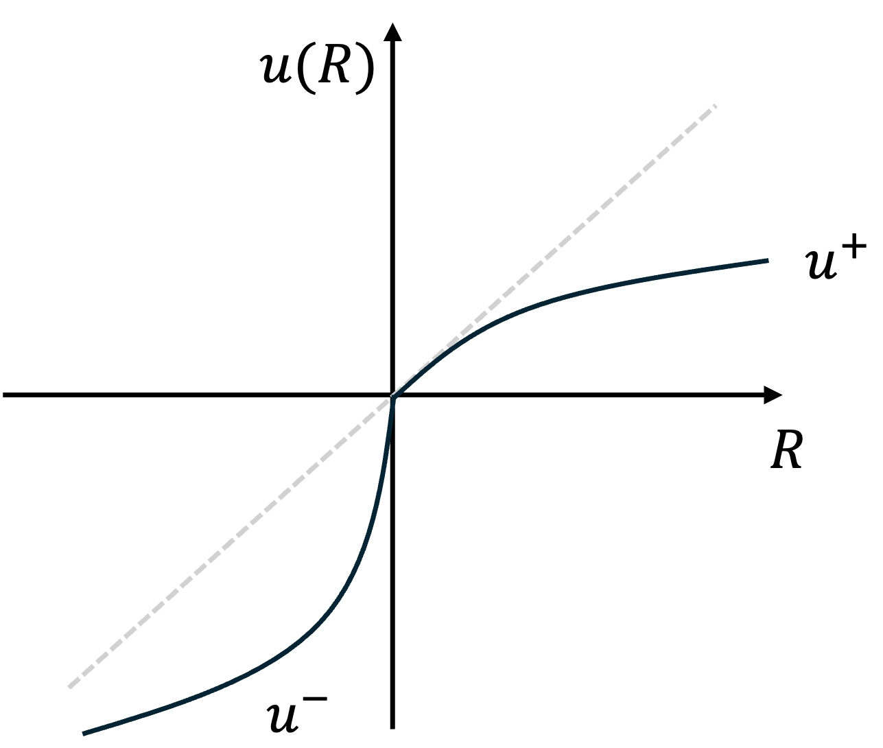
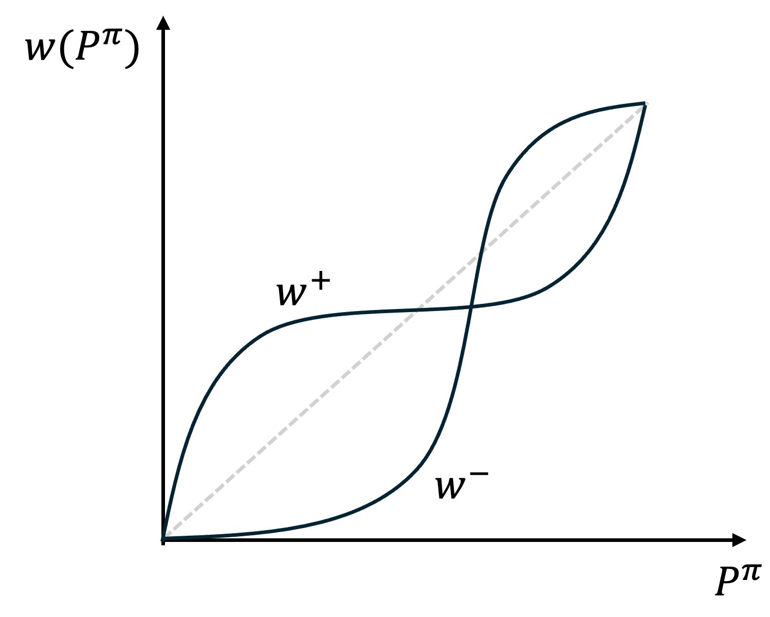
For a random variable , let where denote the indices for the probability of incurring a gain or loss for each . Given a utility function and a weighting function , the Prospect Theory (PT) value is defined as , and the Cumulative Prospect Theory (CPT) value is defined as . Contrary to expected utility theory, which models decisions that perfectly rational agents would make (Rabin (2013)), i.e. , PT seeks to describe the actual behavior of humans, attempting to encompass their irrational decision-making processes. Specifically, PT introduces the concept of probability distortion, where individuals overestimate the likelihood of rare events and underestimate the likelihood of moderate to highly probable events (Figure 1(b)). Value distortion refers to the way individuals assess gains and losses (-axis of Figure 1(a)), often valuing losses more heavily than equivalent gains, which reflects a behavior known as loss aversion (Figure 1(a)) Kahneman and Tversky (2013); Fennema and Wakker (1997). How PT explains human decision-making is well-described in the following example.
Example 4 (Insurance policies).
Consider an example where the probability of an insured risk is %, the potential loss is , and the insurance premium is . According to CPT, most would opt to pay the premium to avoid the larger loss.
Example 4 illustrates how a seemingly straightforward decision can be analyzed as a sequential decision-making problem within a two-step Markov Decision Process framework, where and . The states and represent receiving a loss of , and , respectively. The actions and denote paying and not paying the premium, respectively. At time , humans make a choice between and based on a policy stating at initial state . Choosing results in a guaranteed transition to state . Otherwise, choosing potentially leads to state with a reward of with a probability, or to state with a reward of with a probability. According to the expected utility theorem, which assumes rationality, the estimated value of choosing is calculated as , and the value of choosing as . Rationality would lead humans to prefer since its expected cost is lower than that of , i.e. . However, this choice is counterintuitive and often does not align with real-world human decision making.
CPT uses a similar measure as PT, except that the is a function of cumulative probabilities. The concept involves using an S-shaped utility function, which adheres to the diminishing sensitivity property. If we set the weighting function or utility function to be the identity function, then we retrieve the classical expected utility mode (Rabin (2013)).
5 Agent-Environment intersects as perception
Thus far, we have informally introduced the black swan hypothesis (Hypothesis 1) and spatial black swan definition (Definition 1) in Section 1 and elaborated on its necessity (Subsection 3.1) and supporting evidence (Subsection 3.2) in Section 3. Then, we introduce one existing work to concretize misperception, CPT, in Section 4. In Section 5, we utilize CPT to elaborate the Hypothesis 1 by introducing universe, human, and human-estimation MDP.
5.1 Misperception is information loss
Based on Hypothesis 1, this prompts us to investigate the concept of misperception. Initially, we must clearly define what constitutes perception. In The Quest for a Common Model of the Intelligent Decision Maker, Sutton defines perception as one of four principal components of agents, stating: “The perception component processes the stream of observations and actions to produce the subjective state, a summary of the agent-world interaction so far that is useful for selecting action (the reactive policy), for predicting future reward (the value function), and for predicting future subjective states (the transition model)” Sutton (2022). This definition leads us to consider misperception as the information loss occurring when processing observations into the subjective state, such that the reward and transition model are not equivalent to those from the environment. The interpretation of misperception as information loss during processing is somewhat ambiguous, depending on how the boundary between the agent and the environment is defined. The concept of a boundary between the agent and environment was first proposed by Turing as a ‘skin of an onion’ Turing (2009), and later, Jiang (2019) suggested that algorithms are not boundary-invariant.
Therefore, we propose a new agent-environment framework that incorporates the notion that misperception is the information loss from an agent’s processing. This framework positions perception at the intersection between the agent and the environment. We provide a detailed description of our agent-environment framework in Figure 2 and further elaborate in the following subsection.
5.2 Universe, Human, and Human-Estimation MDP
Restricting the Markov Decision Process introduced in Section 3 in a stationary environment, we consider a single episode finite horizon stationary Markov Decision Process (MDP) denoted as , where represents the state space, denotes the action space, is the transition probability function, is a reward function, is the discount factor, and is a Horizon. We define as the universe MDP and operate under the assumption that the abstraction from the universe to the model is lossless, preserving all relevant information. Given a policy , the agent collects data as it interacts with the environment at discrete time steps . The process starts from a fixed initial state , and we define the value function as follows:
| (1) |
To fully leverage Hypothesis 1, and ‘perception as information loss from agent’s processing’ from subsection 5.1, we define the human MDP where the agent experiences distortions in cumulative distribution of normalized visitation probability and reward function by functions (function characteristics are explained in Assumptions 2 and 3). Note that is the probability of visiting at time by policy starting from .
One internal assumption in the human MDP is that its state and action spaces are the same as those of the universe MDP, i.e. and . This assumption is significant, as insufficient exploration might result in a limited understanding of the entire state space by the human (agent), and the discrepancy between the human MDP and the universe MDP could be considerable, especially in a large discrete state and action space. However, we can augment the human MDP to match with universe MDP by using the following method.
Remark 2.
If humans cannot perceive some state , we can augment the human state space with , define , and set while for all . Thus, the new state does not affect decision-making in a human MDP since the probability that the trajectory visits the state is zero.
From now on, we denote human MDP For a finite state and action space, we can define the order statistics of for and define the cumulative distribution. For short notation, we use as its cumulative distribution. These distortions are defined by the relationships:
| (2) | ||||
| (3) |
We also define the value function of human MDP as follows.
| (4) |
In Equation (2), note that misperceptions are applied to the visitation probability rather than the transition probability itself. This approach is more reasonable, as humans distort the probability of events, and we have defined the dimension of spatial black swan events as (Definition 2). We explore case studies where humans misperceive itself in Section 6. However, we address the following definition and lemma to bridge the gap between these two types of misperceptions, implying that theoretical analyses on one are also interchangeably applicable to the other.
Definition 5 (Biased and perceived reward and visitation).
For given constant , if holds, then is -biased reward. Also, if holds, then is -biased visitation probability. Also, for given constant , if holds, then is -perceived reward. Also, if holds, then is -perceived visitation probability.
Lemma 1.
If where , then the agent can guarantee -perceived visitation probability (See Definition 5 for the definition of -perceived).
Then, the human MDP is fully characterized by the utility functions and the weight functions derived from the universe MDP . We proceed to delineate the properties of these utility and weight functions as described by (Kahneman and Tversky (2013)), under the following assumptions:
Assumption 2 (Utility function).
A function is a non-decreasing concave function that satisfies . A function is a nondecreasing convex function that satisfies .
Assumption 3 (Weight function).
Let be a differentiable function, then those satisfy
-
1.
and .
-
2.
There exists such that .
-
3.
is monotonically decreasing on and monotonically increasing on . Meanwhile, is monotonically increasing on and monotonically decreasing on .
Figure 1 illustrates the geometric properties of the utility and weight functions, as defined under Assumptions 2 and 3. Note that the assumptions concerning the weight functions (Assumption 3) stipulate that and are Lipschitz continuous, with constants and , as derived from the mean value theorem. We denote these constants as and , respectively.
Based on the perceptions of the agent, it executes a trajectory using the policy within the human MDP, , and estimates the perceived reward and visitation probability as and , respectively, from its trajectory. The estimation error bounds are influenced by the complexity of the MDP, including tabular MDPs, linear MDPs, and low-rank MDPs. This configuration is defined as the human-estimation MDP . In a similar way of value function definition in universe MDP as follows.
Based on the definition of Universe MDP, Human MDP, and Human-Estimation MDP, we define their gap as follows, and its relationship could be described as Figure 2.
Since CPT models irrational decision-making, our work begins by defining modified value functions in an infinite-horizon Markov Decision Process (MDP) inspired by CPT. As a preliminary step, we start by defining the CPT-value function in a discrete state and action space.
First, in a discrete state and action space, the value function (Equation (1)) could be expressed as an inner product of reward function and normalized occupancy measure as follows,
| (5) |
Based on Definition 5, the CPT distorts the reward and its visitation probability as follows,
| (6) |
where denotes the value was distorted due to misperception. As one property of CPT is that human perception exhibits distinct distortions of events based on whether the associated rewards are positive or negative, we divide the functions and into where , and where . Assume that the rewards from all state-action pairs are ordered as , and the visitation probability as . Then, CPT-value function is defined as follows:
| (7) |
If we define the reward as the random variable , then we can regard its instance as and its probability as where the probability is dependent on the policy . Suppose that reward function is one to one function. Then the probability denotes the probability of reward and we denote it as . Then, for a reward random variable , expanding the how CPT- applied value function look like in Equation (4), we can define the value function based on continuous state and actions space as follows.
| (8) |
We use the fact that for real-value function , it holds that . In this sense, we define the black swan event in the continuous state and action space.
5.3 Problem setting
Based on three different MDPs, , we consider the following problem setting. The agent rolls out in a single episode with a finite horizon . If the agent has an unbiased perception, then the agent collects a trajectory . However, the agent perceives as and now observe distorted state and reward as where function distorts the state. Now, we can claim the following
Lemma 2.
Suppose the is given. Then, for any function that satisfies the Assumption 3, one can always find the function that satisfies the following equation.
5.4 Utilizing CPT for black swan
We note that existing work on incorporating cumulative prospect theory (CPT) into reinforcement learning, such as (Prashanth et al. (2016); Jie et al. (2018); Danis et al. (2023)), primarily focus on estimating the CPT-based value function and optimizing it to derive an optimal policy. Specifically, (Prashanth et al. (2016); Jie et al. (2018)) demonstrate how to estimate the CPT value function using the Simultaneous Perturbation Stochastic Approximation method and how to compute its gradient for policy optimization algorithms. Additionally, (Shen et al. (2014); Ratliff and Mazumdar (2019)) proposed a novel Q-learning algorithm that applies a utility function to Temporal Difference (TD) errors and demonstrated its convergence. However, these studies (Prashanth et al. (2016); Jie et al. (2018); Danis et al. (2023); Shen et al. (2014); Ratliff and Mazumdar (2019)) do not focus on learning the utility and weight functions, and , but rather assume these as simple functions and focus on how to estimate these functions.
However, this study aims to elucidate the mechanisms by which black swan events arise from the discrepancies between and , despite the agent having perfect estimation, i.e., . As future work, concentrating on devising strategies to reweight the functions , and to mitigate the divergence between the Human MDP and the universe MDP is suggested as a way to achieve antifragility.
6 Case study: how optimal decision deviates under irrationality
So far, we have informally introduced the black swan hypothesis (Hypothesis 1) and spatial black swans (Definition 1) in Section 1, then elaborated on its necessity (Subsection 3.1) and provided evidence (Subsection 3.2) in Section 3. Subsequently, in Section 4, we introduced the Cumulative Prospect Theorem (CPT) to model human irrationality. In Section 5, we incorporated CPT into the Markov Decision Process (Subsection 5.2), viewed through the lens of existing work on defining perception (Subsection 5.1) by introducing universe, human, and human-estimation MDPs (Figure 2).
Given our main hypothesis that black swan events occur due to human misperception of the real world, we further investigate whether optimal policy also deviates due to misperceptions of value or probability. This is critical as overestimating or underestimating all values of probability does not necessarily lead to changes in optimal policy. For example, revisiting Example 4, overestimating or underestimating to the same magnitude does not alter the optimal policy for a human to choose . More fundamentally, a crucial question that this paper addresses is how misperception influences the deviation of optimal policy. Therefore, in Section 6, we first present some case studies in MDPs with small complexity to demonstrate how optimal policy varies under misperception.
Before proceeding, we need to establish the core event of subjective probability. For example, while agents (humans) might distort transition probabilities and perceive them subjectively at a low level which is an intuitive way to model misperception. It is essential to recall that in the Markov Decision Process, the quality of an event is revealed through rewards defined over specific states and actions. This suggests that it is more reasonable to define the minimal object (event) as the state and action, and conduct modeling as distortion on the visitation probability of state and action rather than on the transition probability itself. Since this approach has not been investigated in existing work, we examine both cases in Section 6 and Section 7. Specifically, in Section 6, we assume distortion of transition probability within a non-stationary Markov decision process and investigate how optimal policy deviates due to misperception of transition probability. Then, in Section 7, we explore the distortion of the visitation probability within a stationary Markov decision process.
6.1 Problem setup for Section 6
In this section, we consider discrete state and action stationary Markov Decision Process. Build upon value function (Equation 4), we define value function and state value function of time as
| (9) | ||||
and define the optimal policy as time as . Then the following bellman equation holds,
where holds. In addition, we assume that and . We only consider the reward function at the final stage . Although this assumption may appear unconventional, it aligns with standard practices in reinforcement learning, especially when focusing on terminal rewards. Especially, for each trajectory , where represents a -step decision sequence, set the terminal reward as , and for all
6.2 Case 1. Contextual bandit ()
We begin with a simple case where the decision horizon is , commonly referred to as a contextual bandit (Lattimore and Szepesvári (2020)). Surprisingly, in this setting, the human optimal policy coincides with the real-world optimal policy. This is somewhat counterintuitive, as several significant examples (Examples 2, 3, and 4) suggest that human decision-making often exhibits irrationality.
Theorem 1 (One-step Human Optimal Policy).
If , then the optimal policy from the universe MDP aligns with the optimal policy of the human MDP, i.e. .
An important insight from Theorem 1 is that when decisions are not sequential, the typical distortions in human perception do not affect the alignment with the optimal policy of the real-world, suggesting that human irrationality is less influential in a single-step decision-making setting. This is further explained in the following remark.
Remark 3.
Continuing from Example 4, the order of perceived rewards does not change as since is a nondecreasing convex function.
6.3 Case 2. when
Now, let us consider the simplest case where where . Surprisingly, we find results similar to those presented in Section
Theorem 2 (Multi-step human optimal policy).
If , then the optimal policy from the universe MDP also aligns with the optimal policy of the human MDP, that is, for .
The proof of Theorem 2 is based mainly on the assumption that , notably using the property that . However, this technique cannot be applied directly if . For example, in Example 4, where , it is demonstrated that human decision making results in a suboptimal policy in the real-world. This outcome may seem counterintuitive. However, a heuristic analysis suggests that having only two states in the state space indicates that the actions do not introduce a varied randomness. Essentially, if randomness is introduced by any action, it would likely affect both states and if the action provides a nondeterministic next state. Thus, every action provides the same next-state set, which makes a mere comparison between two states. This observation implies that in scenarios with a smaller state space, being irrational (believing on false belief) does not affect to deviate from optimal policy. We can also interpret this result as if is small, sequential decision-making problems are easy so that humans can always provide the optimal action in the real world.
6.4 Case 3: with unbiased reward perception
We consider the hypothetical scenario where , indicating that humans have an unbiased perception of their reward.
Theorem 3 (Two step optimal decision when ).
Given any state space where and a decision horizon , there exists a transition probability and reward of the real world such that the optimal policy of human MDP differs from that of universe MDP.
7 A definition of spatial black swans
Now, we introduce the definition of black swan inspired by CPT.
7.1 Black swan hypothesis
First, based on the newly proposed human model , we concretize the informal hypothesis 1 as follows.
We define all spatial black swan events as a set . It is important to note that is a function of the agent’s perception , rather than its estimation , since estimation is what the agent can improve over time. Specifically, all state and action events from can be regarded as broad ‘risks’ that encompass spatial black swan events. Among these risks, there are some that the agent can ‘be averse to’ and others that it ‘cannot be averse to’ in the process of improving model estimation to the human model . The crux of spatial black swan events lies in their unexpectedness, which occurs even when the agent has prepared the optimal policy with zero estimation error. The model estimation process discussed in this paper aligns with existing work on imperfect model-based reinforcement learning (Jiang (2018); Gheshlaghi Azar et al. (2013); Fard and Pineau (2010); Agarwal et al. (2020); Lecarpentier and Rachelson (2019)). For future work, we leave room to define the ‘risks’ due to irrational human behavior that goes beyond spatial black swans. Specifically, events from are risk events that can be avoided as time goes by, and events from are non-avoidable risk, i.e. spatial black swans. This conceptual framework can be outlined by the following equation:
| (10) |
Equation (10) is supported by Definition 5, where leads to and . This implies that converges to by the definitions of the Human MDP and the Human-Estimation MDP, and consequently, converges to .
7.2 A definition of spatial black swans
As a preliminary step, we define spatial black swan events within a discrete state and action space. Note that we continue the problem setting that is discussed in deriving Equation (7) in Subsection 5.2.
Definition 6 (Spatial black swan - discrete state and action space).
Among the indices of order statistics, if index meets the following criteria:
-
1.
.
-
2.
, yet .
where and is given a constant, we define as a spatial black swan event.
The property of Definition 6 identifies a ‘high-risk event’ through the function gap between the universe reward from and the perceived reward from . Specifically, if the agent perceives in a pessimistic way such that , this is considered a high-risk event resulting from misperception. The property of Definition 6 also characterizes a ‘rare event’ through a lens of misperception. Technically, it describes that a spatial black swan event feasibly occurs in the universe (), but the agent perceives it as nonoccurring (), i.e. an infeasible event.
In addition, we denote two parameters, and , to represent the extent of distortion in the reward and the cumulative probability of visitation. Intuitively, the magnitude of and is related to the extent of the misperception gap between and ,i.e. . We elaborate on this conjecture in Theorem 4 of Section 8. We now extend the definition of black swan events from discrete state and action spaces to continuous spaces as follows.
Definition 7 (Spatial black swan).
Given , if the state-action pair satisfies the following conditions:
-
1.
.
-
2.
but .
where represents the cumulative distribution function of , then we define that state and action pair as a black swan event.
If the weight function is differentiable, then the property of spatial black swan events can be further elaborated as follows: The derivative , yet the probability density distribution remains non-zero and bounded, specifically . Consequently, this implies . This refined second property will be utilized to extend the definition of spatial black swan events to Proposition 3 in Section 8, facilitating further analysis (see Figure 3(b)).
Also, for all functions that prevent the existence of spatial black swan events, i.e., , we refer to such environments as safe perception, denoted by . In contrast, environments characterized by that inherently encompass spatial black swan events, , are termed risk perception environments. Specifically, if an agent perceives the world through , then spatial black swan events are absent; however, it is crucial to recognize that are not unique functions (see Figure 3(b)).
8 Theoretical analysis of spatial black swans
Thus far, we have elaborated on the definition of spatial black swan events (Definition 7) from its informal definition (Definition 1) through the lens of our black swan hypothesis (Hypothesis 2). In this section, we provide theoretical analysis that quantifies the impact of spatial black swan events. Specifically, we demonstrate how the existence of spatial black swans establishes a lower bound on policy performance (Theorem 4), and assesses the probability of encountering spatial black swan events over time (Theorem 5). It is important to note that Theorem 5 serves as a critical precursor to characterizing the third property of the informal proposition (Proposition 2), since the timing of learning to improve agent’s perception is triggered by the statement ‘after a black swan is first observed’. Subsequently, we posit that perception improvement learning exhibits antifragile behavior in agents.
8.1 Problem setting
As a preliminary step, we first establish the agent learning setting and provide some assumptions for the theoretical analysis. We utilize the problem setting elaborated in Subsection 5.3. For the theoretical analysis, we assume the following assumptions:
Assumption 4 (Bounded reward).
The is bounded as where
Assumption 5 (Relatively strong convexity).
With Assumption 2, holds for .
Before starting the theoretical analysis, the formal definition of spatial black swan events based on state and action pairs (Definition 7) imposes restrictions on further analysis due to the openness of . Specifically, Definition 7 regarding the support of does not ensure the existence of a closed subset such that . Therefore, we propose modifications to the support of the spatial black swan event definition concerning the reward. To this end, we further assume that the reward function is bijective. Consequently, we introduce the following proposition of a spatial black swan event, an alternative to Definition 7, which is defined over reward values in closed intervals.
Proposition 3 (Spatial black swan).
Under Assumptions 1,2, and 3, if satisfies spatial black swan definition (Definition 7), then satisfies
-
1.
-
2.
but
where holds.
The Proposition 3 is well elaborated in Figure 3. Proposition 3 facilitates the Definition 7 within the closed set . This approach to defining spatial black swan events based on the support of the reward is more intuitive to understand the black swan origin hypothesis (Hypothesis 2). That is, Proposition 3 shows how decreasing the misperception gap () relates to reducing . This is because a reduction in the misperception gap, where , leads to a decrease in the range of spatial black swan rewards, moving from to , thus reducing the frequency of spatial black swan occurrences (see Figure 3).
Within the above problem setting, the agent’s goal is to estimate the value function under safe perception as follows:
| (11) |
However, the agent possesses its own perceptions , for which we assume the risk perception is represented as:
| (12) |
As time goes by, the agent’s goal is learning the weight functions and utility functions such as and . Then, by the single trajectory data up to time , i.e. where the reward value itself and its sampling distribution are distorted due to the functions and , respectively. Let denote samples of the reward random variable . We define the empirical distribution function for and as follows
. using the EDFs, the CPT value up to time can be estimated as follows,
| (13) |
Again, we note that the gap between and is defined over a gap between and that is proportional to the existence of spatial black swan events.


8.2 Theortical analysis
Based on the perspective of the blackswan event as a reward (Proposition 3), the natural question would be how does the perception gap create a gap between the value function?
Theorem 4 (Convergence of estimation value but lower bound on perceived value gap).
Under Assumptions 2, 3, and 4, the asymptotic convergence of the value function estimation holds as follows,
| (14) |
where upper bound of the estimation error (sample complexity) holds as:
| (15) |
where .
However, under specific conditions on , the lower bound of human value function gap is expressed as:
| (16) |
due to misperception.
Insights of Theorem 4. The message of Theorem 4 establishes a support for our hypothesis 2 and Defintion 7. Firstly, Equation (15) establishes that the estimation error converges to zero as the agent rolls out a longer trajectory. However, Equation (16) offers the insight that the value function gap between and has a lower bound, regardless of the trajectory length. It is straightforward to verify in Equation (16) that if and , which implies and , then the lower bound also converges to zero. Furthermore, Equation (16) supports our intuition that a higher distortion in reward perception (a large value) and a greater number of spatial black swan events (large ) and a large minimum probability of spatial black swan event occurrence (large ) lead to a higher lower bound. It is important to note that the gap is associated with the number of spatial black swans, since we have assumed that the reward function maps uniquely, therefore there exists a unique such that , where is in the range . Therefore, through Theorem 4, we conclude that even though the agent has a perfect estimation of what it has perceived, there still exists a lower bound to obtaining the value function of the universe, which increases as the parameter effect of spatial black swan events becomes more dominant.
Now, based on Theorem 4, the next natural question is how to decrease the lower bound, that is, how the agent learns to nudge and . Before we ask when the agent encounters the black swan, so the perception correction would happen. Since black swan events are defined over probability, this question could be more concretized as If the agent takes a step , the probability of encountering black swan events are at least . This question also further enables to naturally learn how to obtain antifragile behavior, which makes to decrease as every time the agent updates its perception. We first start our analysis based on the non-zero one-step reachability assumption.
Theorem 5 (Spatial black swan hitting time).
Assume for any two states , signifying that the one-step state reachability is non-zero, and consider that one step corresponds to a unit time. Then, if the agent takes steps such that
where and , it will encounter spatial black swan events at least with probability .
9 Conclusion
In this paper, we propose a new perspective to understand the black swan events by utilizing human misperception and CPT. We have divided black swans into temporal and spatial black swans and focus on spatial black swans, where misperception occurs in the state and action space. To define spatial black swans, we propose three different MDPs: universe MDP (), human MDP (), and human-estimation MDP () and also introduce the well-known irrational human behavior theorem, CPT. The main message is Hypothesis 2 and Definition 7. They highlight that despite humans being able to reduce the estimation gap, leading to converge to through longer horizons or better algorithms, there remains an inherent uncertainty due to the perception gap between and . This implies that spatial black swans can still occur because of this perception gap, even when the agent has zero estimation error and computes its optimal policy from .
Acknowledgments and Disclosure of Funding
We thank Jason Jangho Choi for providing instructive insights on the early draft, and Donghao Ying for discussions on mathematical notation. The authors also thank Theophane Weber and Csaba Szepesvari and the rest of the Google DeepMind team who reviewed the paper.
Appendix A Proofs
Lemma 3 (Bounding visitation probability of step when well-perceived transition holds).
If for all holds -perceived transition probability, then we have
that holds for all
Proof of Lemma 3.
Proof by induction. We use short notation for as and as . By the definition of rational transition probability the statement holds at for any policy . Now, suppose the statement holds for for any policy . Then, we have
The all of above inequalities holds for all . Therefore, the statement holds for all . ∎
Now, we state the proof of Lemma 1.
Proof of Lemma 1.
Proof of Lemma 2.
First, note that we have assumed the image of the function is closed and dense as . Then, in the progress of projecting all into the reward, we define the probability of reward as . we use short notation for as . Now, since is the visitation probability of visiting , then this could be converted to by where is many to one function.
Now, since is the many to one function, we can define independent block the as the set . Note that if , then . Then, if satisfies the set to in be permutation- invariant. Namely, if , then holds then there exists a one-to-one mapping function such that
holds. The proof can be divided into two folds. The existence of such function and its a one-to-one mapping function is exists. We first prove the existence of such function . This is because for any state and action , suppose its reward value as . Then suppose . Then since image of function is closed and dense, there exists such that holds. Then, one can say the function exists. Now, we prove the one-to-one mapping property. suppose for two state and action pair and and let and . Now, suppose holds. Then, due to the property of , then it should also satisfies . Therefore, this concludes that is the one-to-one mapping, and the following holds
holds. we denote as . Then, let’s define two different functions and such that we want to claim that
| (17) |
holds for any . Since the proof for either is similar, we prove the case for the existence of under distortion.
Now, recall that for , holds and for , holds and is monotically increasing function. Define such that holds, and for notation simplicity we deonte . Then, one can say , holds and. Then we can always find a unique ratio that depends on such that holds where
Proof of Theorem 1.
By the definition of optimal policy and the value function definition at the time , we have the optimal policy at time as follows.
for any fixed , let’s assume is the argument that maximizes the . Since is the non-decreasing convex function, is still the same argument that maximizes the . Therefore, holds. ∎∎
Proof of Theorem 2.
We prove by backward induction. First by theorem 1, holds. Now suppose that holds for all . Now, we prove the statement holds for . To prove , it is sufficient to show if , then also holds for any actions . First, the gap could be expressed as
and as
the reward during is zero by our problem formulation assumption in section 6.1. Now, without loss of generality, we assume . Then, due to our assumption that holds for , we also have . Also, noticing that weight function is also increasing function, then also guarantees holds. Therefore, we can claim if holds, then also holds. Then, this leads to claim that , which implies . This completes the proof. ∎∎
Proof of Theorem 3.
Assume that Theorem 3 does not hold. Given , we have for each state . At time , assume . The condition is then expressed as:
which simplifies to:
For the non-distorted case, the analogous expression is:
For arbitrary reward functions, , the equality of the two cases under any weighting function leads to:
where is the only solution, contradicting the distortion required by Assumption 3. ∎
Proof of Theorem 4.
The proof of Theorem 4 is divided into three-fold.
1. Proof of asymptotic convergence
We first prove asymptotic convergence (Equation (14)), then we prove Equation (15) in part 3 of this proof. Note that the empirical distribution function generate Stielgies measure which takes mass each of the sample points on .
or equivalently, show that
| (18) |
where denotes the number of positive reward among . Let and denote the th quantile of and , respectively.
For the convergence proof, we first concentrate on finding the following probability,
| (19) |
for any given . It is easy to check that
| (20) | |||
| (21) |
The Right hand side of Inequality (21) could be expressed as follows.
We focus on the term . Now, let us define an event where . Since the Cumulative distribution is non-decrasing function, we have the following,
Using the fact that in conjunction with Hoeffding’s inequality, we obtain
| (22) |
where . Since is Lipschitz, we have that . Hence, we obtain
| (23) |
In a similar fashion, one can show that
| (24) |
Combining (23) and (24), we obtain
Plugging the above in (21), we obtain
| (25) |
Notice that since the sequence will decrease more rapidly than the sequence , .
Also, the remaining part, conducting the proof of convergence of and ,i.e.
| (26) |
also follows simliar manner. we omit the proof for this.
2. Proof of value function lower bound
By the definition, we have the following
We first under bound the term (I). For notation simplicity, we let and . Then we have the following
| Term (I) |
Now, since is monotonically increasing in and monotonically decreasing in , we could say for any that
where . The first equality holds due to the mean value theorem. Therfore it holds that
| Term (I) | |||
Now, recall the definition of and , then we have the following
Now, let us denote the intersection of and as . We can say if the blackswan happens, then its reward is bounded between . Then we have the following,
To lower bound the Term I-1, let’s denote the minimum reachability of blackswan events as . Then we have
| Term I-1 | ||||
| (27) |
| Term I-2 | ||||
| (28) |
Therefore, we have the following equation,
Also, since the function is convex, and holds. Therefore, we could say . This leads us to come up with . Therefore, we have a gap lowerbound as
The above inequality could be minimized as
| Term I | |||
Now, let’s upper bound Term 2. Before, recall that the definition of and note that by the definition of black swans, we have holds for . Therefore, we can say for all holds. Therefore, for all , we have
| (29) |
Note that if , then
| (30) |
and if , then
| (31) |
Therefore, combining the Equations (29), (30), (31), we conclude that
where is a constant. This completes the proof.
3. Value function upper bound
For the proof of Equation (15) of Theorem 4, we utilized the following Lemma 4 which provides a concentration inequality on the distance between empirical distribution and true distribution.
Since is bounded above by and is Lipschitz with constant , we have the following inequality,
Now, plugging in the DKW inequality, we obtain
| (32) |
Along similar manner, we have
| (33) |
∎∎
Proof of Theorem 5.
For a given optimal policy , define the normalized occupancy measure as . Note that represents the stationary distribution. Additionally, given the assumption that the reward function is a bijection, it follows that the distribution and are identical. This indicates that the occurrence of black swan events can be entirely characterized by the reward values, rather than the specific state-action pairs.
Now, we define the event where . The probability of event happens is bounded as follows
Note that we have assumed the and its minimum reachable probability as for all reward. now, for given trajectory, the reward instance is given as where , the probability that the agent first visit the black swan event at step would be defined as
Therefore, its probability is bounded as follows,
Now, to ensure that the blackswan probability to be lower bounded than , we need the following conditions,
Therefore, we have
Therefore, we can conclude that if , then the agent’s probability to meet the black swan is at least .
∎∎
Appendix B Helpful Lemmas
Lemma 4.
(Dvoretzky-Kiefer-Wolfowitz (DKW) inequality)
Let denote the empirical distribution of a r.v. , with being sampled from the r.v .
The, for any and , we have
References
- Abel et al. (2024) D. Abel, A. Barreto, B. Van Roy, D. Precup, H. P. van Hasselt, and S. Singh. A definition of continual reinforcement learning. Advances in Neural Information Processing Systems, 36, 2024.
- Agarwal et al. (2020) A. Agarwal, S. Kakade, and L. F. Yang. Model-based reinforcement learning with a generative model is minimax optimal. In Conference on Learning Theory, pages 67–83. PMLR, 2020.
- Agrawal et al. (2021) S. Agrawal, S. K. Juneja, and W. M. Koolen. Regret minimization in heavy-tailed bandits. In Conference on Learning Theory, pages 26–62. PMLR, 2021.
- Bagnell et al. (2001) J. A. Bagnell, A. Y. Ng, and J. G. Schneider. Solving uncertain markov decision processes. 2001.
- Barandiaran et al. (2009) X. Barandiaran, E. D. Paolo, and M. Rohde. Defining agency: Individuality, normativity, asymmetry, and spatio-temporality in action. Adaptive Behavior, 17(5):367–386, 2009.
- BetterUp (2022) BetterUp. The availability heuristic. https://www.betterup.com/blog/the-availability-heuristic, 2022. Accessed: 2024-05-12.
- Bowling et al. (2023) M. Bowling, J. D. Martin, D. Abel, and W. Dabney. Settling the reward hypothesis. In International Conference on Machine Learning, pages 3003–3020. PMLR, 2023.
- Bradley and Taqqu (2003) B. O. Bradley and M. S. Taqqu. Financial risk and heavy tails. In Handbook of heavy tailed distributions in finance, pages 35–103. Elsevier, 2003.
- Bubeck et al. (2013) S. Bubeck, N. Cesa-Bianchi, and G. Lugosi. Bandits with heavy tail. IEEE Transactions on Information Theory, 59(11):7711–7717, 2013.
- Carr et al. (2024) J. C. Carr, P. Panangaden, and D. Precup. Conditions on preference relations that guarantee the existence of optimal policies. In International Conference on Artificial Intelligence and Statistics, pages 3916–3924. PMLR, 2024.
- Chung and Sobel (1987) K.-J. Chung and M. J. Sobel. Discounted mdp’s: distribution functions and exponential utility maximization. Siam Journal on Control and Optimization, 25:49–62, 1987. URL https://api.semanticscholar.org/CorpusID:119760011.
- Coraluppi (1997) S. P. Coraluppi. Optimal control of Markov decision processes for performance and robustness. University of Maryland, College Park, 1997.
- Coraluppi and Marcus (1999) S. P. Coraluppi and S. I. Marcus. Risk-sensitive and minimax control of discrete-time, finite-state markov decision processes. Automatica, 35(2):301–309, 1999.
- Coraluppi and Marcus (2000) S. P. Coraluppi and S. I. Marcus. Mixed risk-neutral/minimax control of discrete-time, finite-state markov decision processes. IEEE Transactions on Automatic Control, 45(3):528–532, 2000.
- Danis et al. (2023) D. Danis, P. Parmacek, D. Dunajsky, and B. Ramasubramanian. Multi-agent reinforcement learning with prospect theory. In 2023 Proceedings of the Conference on Control and its Applications (CT), pages 9–16. SIAM, 2023.
- Delage and Mannor (2010) E. Delage and S. Mannor. Percentile optimization for markov decision processes with parameter uncertainty. Operations research, 58(1):203–213, 2010.
- Di Castro et al. (2012) D. Di Castro, A. Tamar, and S. Mannor. Policy gradients with variance related risk criteria. arXiv preprint arXiv:1206.6404, 2012.
- Dong et al. (2022) S. Dong, B. Van Roy, and Z. Zhou. Simple agent, complex environment: Efficient reinforcement learning with agent states. Journal of Machine Learning Research, 23(255):1–54, 2022.
- Drakopoulos and Theodossiou (2016) S. A. Drakopoulos and I. Theodossiou. Workers’ risk underestimation and occupational health and safety regulation. European Journal of Law and Economics, 41:641–656, 2016.
- Fard and Pineau (2010) M. Fard and J. Pineau. Pac-bayesian model selection for reinforcement learning. Advances in Neural Information Processing Systems, 23, 2010.
- Fennema and Wakker (1997) H. Fennema and P. Wakker. Original and cumulative prospect theory: A discussion of empirical differences. Journal of Behavioral Decision Making, 10(1):53–64, 1997.
- Fleming and Sarkar (2014) M. J. Fleming and A. Sarkar. The failure resolution of lehman brothers. Economic Policy Review, Forthcoming, 2014.
- Garcıa and Fernández (2015) J. Garcıa and F. Fernández. A comprehensive survey on safe reinforcement learning. Journal of Machine Learning Research, 16(1):1437–1480, 2015.
- Geibel (2006) P. Geibel. Reinforcement learning for mdps with constraints. In Machine Learning: ECML 2006: 17th European Conference on Machine Learning Berlin, Germany, September 18-22, 2006 Proceedings 17, pages 646–653. Springer, 2006.
- Geibel and Wysotzki (2005) P. Geibel and F. Wysotzki. Risk-sensitive reinforcement learning applied to control under constraints. Journal of Artificial Intelligence Research, 24:81–108, 2005.
- Gheshlaghi Azar et al. (2013) M. Gheshlaghi Azar, R. Munos, and H. J. Kappen. Minimax pac bounds on the sample complexity of reinforcement learning with a generative model. Machine learning, 91:325–349, 2013.
- Gilovich et al. (2002) T. Gilovich, D. Griffin, and D. Kahneman. Heuristics and biases: The psychology of intuitive judgment. Cambridge university press, 2002.
- Gosavi (2009) A. Gosavi. Reinforcement learning for model building and variance-penalized control. In Proceedings of the 2009 winter simulation conference (wsc), pages 373–379. IEEE, 2009.
- Heger (1994) M. Heger. Consideration of risk in reinforcement learning. In Machine Learning Proceedings 1994, pages 105–111. Elsevier, 1994.
- Hendrycks et al. (2021) D. Hendrycks, N. Carlini, J. Schulman, and J. Steinhardt. Unsolved problems in ml safety. arXiv preprint arXiv:2109.13916, 2021.
- Housel (2023) M. Housel. Penguin, 2023.
- Howard and Matheson (1972) R. A. Howard and J. E. Matheson. Risk-sensitive markov decision processes. Management science, 18(7):356–369, 1972.
- Huisman et al. (1998) R. Huisman, K. G. Koedijk, and R. A. Pownall. Var-x: Fat tails in financial risk management. Journal of risk, 1(1):47–61, 1998.
- Iyengar (2005) G. N. Iyengar. Robust dynamic programming. Mathematics of Operations Research, 30(2):257–280, 2005.
- Jiang (2018) N. Jiang. Pac reinforcement learning with an imperfect model. In Proceedings of the AAAI Conference on Artificial Intelligence, volume 32, 2018.
- Jiang (2019) N. Jiang. On value functions and the agent-environment boundary. arXiv preprint arXiv:1905.13341, 2019.
- Jie et al. (2018) C. Jie, L. Prashanth, M. Fu, S. Marcus, and C. Szepesvári. Stochastic optimization in a cumulative prospect theory framework. IEEE Transactions on Automatic Control, 63(9):2867–2882, 2018.
- Kahneman and Tversky (2013) D. Kahneman and A. Tversky. Prospect theory: An analysis of decision under risk. In Handbook of the fundamentals of financial decision making: Part I, pages 99–127. World Scientific, 2013.
- Lattimore and Szepesvári (2020) T. Lattimore and C. Szepesvári. Bandit algorithms. Cambridge University Press, 2020.
- Lecarpentier and Rachelson (2019) E. Lecarpentier and E. Rachelson. Non-stationary markov decision processes, a worst-case approach using model-based reinforcement learning. Advances in neural information processing systems, 32, 2019.
- Lee et al. (2024) H. Lee, Y. Ding, J. Lee, M. Jin, J. Lavaei, and S. Sojoudi. Tempo adaptation in non-stationary reinforcement learning. Advances in Neural Information Processing Systems, 36, 2024.
- Leqi et al. (2019) L. Leqi, A. Prasad, and P. K. Ravikumar. On human-aligned risk minimization. Advances in Neural Information Processing Systems, 32, 2019.
- Martino et al. (2006) B. D. Martino, D. Kumaran, B. Seymour, and R. J. Dolan. Frames, biases, and rational decision-making in the human brain. Science, 313:684 – 687, 2006.
- Mawutor (2014) J. K. M. Mawutor. The failure of lehman brothers: causes, preventive measures and recommendations. Research Journal of Finance and Accounting, 5(4), 2014.
- McDonald and Robinson (2009) L. McDonald and P. Robinson. A colossal failure of common sense: The incredible inside story of the collapse of Lehman Brothers. Random House, 2009.
- Moldovan and Abbeel (2012) T. Moldovan and P. Abbeel. Risk aversion in markov decision processes via near optimal chernoff bounds. Advances in neural information processing systems, 25, 2012.
- Neummann and Morgenstern (1944) J. Neummann and O. Morgenstern. Theory of games and economic behaviour, 1944.
- Nilim and El Ghaoui (2005) A. Nilim and L. El Ghaoui. Robust control of markov decision processes with uncertain transition matrices. Operations Research, 53(5):780–798, 2005.
- Opaluch and Segerson (1989) J. J. Opaluch and K. Segerson. Rational roots of “irrational” behavior: new theories of economic decision-making. Northeastern Journal of Agricultural and Resource Economics, 18(2):81–95, 1989.
- Orseau and Ring (2012) L. Orseau and M. Ring. Space-time embedded intelligence. In Artificial General Intelligence: 5th International Conference, AGI 2012, Oxford, UK, December 8-11, 2012. Proceedings 5, pages 209–218. Springer, 2012.
- Osogami (2012) T. Osogami. Robustness and risk-sensitivity in markov decision processes. Advances in Neural Information Processing Systems, 25, 2012.
- Pandit et al. (2019) B. Pandit, A. Albert, Y. Patil, and A. J. Al-Bayati. Impact of safety climate on hazard recognition and safety risk perception. Safety science, 113:44–53, 2019.
- Patek (2001) S. D. Patek. On terminating markov decision processes with a risk-averse objective function. Automatica, 37(9):1379–1386, 2001.
- Pitis (2024) S. Pitis. Consistent aggregation of objectives with diverse time preferences requires non-markovian rewards. Advances in Neural Information Processing Systems, 36, 2024.
- Ponda et al. (2013) S. S. Ponda, L. B. Johnson, and J. P. How. Risk allocation strategies for distributed chance-constrained task allocation. In 2013 American Control Conference, pages 3230–3236. IEEE, 2013.
- Prashanth et al. (2016) L. Prashanth, C. Jie, M. Fu, S. Marcus, and C. Szepesvári. Cumulative prospect theory meets reinforcement learning: Prediction and control. In International Conference on Machine Learning, pages 1406–1415. PMLR, 2016.
- Rabin (2013) M. Rabin. Risk aversion and expected-utility theory: A calibration theorem. In Handbook of the fundamentals of financial decision making: Part I, pages 241–252. World Scientific, 2013.
- Ratliff and Mazumdar (2019) L. J. Ratliff and E. Mazumdar. Inverse risk-sensitive reinforcement learning. IEEE Transactions on Automatic Control, 65(3):1256–1263, 2019.
- Rogers (1998) P. Rogers. The cognitive psychology of lottery gambling: A theoretical review. Journal of gambling studies, 14(2):111–134, 1998.
- Savage (1972) L. J. Savage. The foundations of statistics. Courier Corporation, 1972.
- Shakerinava and Ravanbakhsh (2022) M. Shakerinava and S. Ravanbakhsh. Utility theory for sequential decision making. In International Conference on Machine Learning, pages 19616–19625. PMLR, 2022.
- Shen et al. (2014) Y. Shen, M. J. Tobia, T. Sommer, and K. Obermayer. Risk-sensitive reinforcement learning. Neural computation, 26(7):1298–1328, 2014.
- Simon (1993) H. A. Simon. Decision making: Rational, nonrational, and irrational. Educational administration quarterly, 29(3):392–411, 1993.
- Sugden (1991) R. Sugden. Rational choice: a survey of contributions from economics and philosophy. The economic journal, 101(407):751–785, 1991.
- Sunehag and Hutter (2011) P. Sunehag and M. Hutter. Axioms for rational reinforcement learning. In Algorithmic Learning Theory: 22nd International Conference, ALT 2011, Espoo, Finland, October 5-7, 2011. Proceedings 22, pages 338–352. Springer, 2011.
- Sunehag and Hutter (2015) P. Sunehag and M. Hutter. Rationality, optimism and guarantees in general reinforcement learning. The Journal of Machine Learning Research, 16(1):1345–1390, 2015.
- (67) R. S. Sutton. The reward hypothesis, 2004. URL http://incompleteideas. net/rlai. cs. ualberta. ca/RLAI/rewardhypothesis. html.
- Sutton (2022) R. S. Sutton. The quest for a common model of the intelligent decision maker. arXiv preprint arXiv:2202.13252, 2022.
- Taha (2007) H. A. Taha. Operations research an introduction. 2007.
- Taleb (2010) N. N. Taleb. The Black Swan:: The Impact of the Highly Improbable: With a new section:” On Robustness and Fragility”, volume 2. Random house trade paperbacks, 2010.
- Turing (2009) A. M. Turing. Computing machinery and intelligence. Springer, 2009.
- van der Meer et al. (2022) T. G. van der Meer, A. C. Kroon, and R. Vliegenthart. Do news media kill? how a biased news reality can overshadow real societal risks, the case of aviation and road traffic accidents. Social forces, 101(1):506–530, 2022.
- Vasterman et al. (2005) P. Vasterman, C. J. Yzermans, and A. J. Dirkzwager. The role of the media and media hypes in the aftermath of disasters. Epidemiologic reviews, 27(1):107–114, 2005.
- Wahlberg and Sjoberg (2000) A. A. Wahlberg and L. Sjoberg. Risk perception and the media. Journal of risk research, 3(1):31–50, 2000.
- Wheeler and Wheeler (2007) G. Wheeler and G. Wheeler. A review of the lottery paradox. Probability and inference: Essays in honour of Henry E. Kyburg, Jr, pages 1–31, 2007.
- Wiesemann et al. (2013) W. Wiesemann, D. Kuhn, and B. Rustem. Robust markov decision processes. Mathematics of Operations Research, 38(1):153–183, 2013.
- Xu and Mannor (2010) H. Xu and S. Mannor. Distributionally robust markov decision processes. Advances in Neural Information Processing Systems, 23, 2010.
- Zhang et al. (2018) Y. Zhang, X. Li, and S. Guo. Portfolio selection problems with markowitz’s mean–variance framework: a review of literature. Fuzzy Optimization and Decision Making, 17:125–158, 2018.
