Covariate Assisted Entity Ranking with Sparse Intrinsic Scores ††thanks: Emails: jqfan@princeton.edu, jikaih@princeton.edu, and mengxiny@wharton.upenn.edu. Research is supported by NSF grants DMS-2210833 and DMS-2053832, and ONR grant N00014-22-1-2340
Abstract
This paper addresses the item ranking problem with associate covariates, focusing on scenarios where the preference scores can not be fully explained by covariates, and the remaining intrinsic scores, are sparse. Specifically, we extend the pioneering Bradley-Terry-Luce (BTL) model by incorporating covariate information and considering sparse individual intrinsic scores. Our work introduces novel model identification conditions and examines the statistical rates of the regularized penalized Maximum Likelihood Estimator (MLE). We then construct a debiased estimator for the penalized MLE and analyze its distributional properties. Additionally, we apply our method to the goodness-of-fit test for models with no latent intrinsic scores, namely, the covariates fully explaining the preference scores of individual items. We also offer confidence intervals for ranks. Our numerical studies lend further support of our theoretical findings, demonstrating validation for our proposed method.
1 Introduction
Ranking plays an essential role across a wide scope of domains. Specifically, it holds particular significance in many real-world applications, including individual choice (Luce, 2005), ranking web pages (Dwork et al., 2001), recommendation systems (Baltrunas et al., 2010; Li et al., 2019), education (Caron et al., 2014), sports ranking (Massey, 1997; Turner and Firth, 2012), scientific journals ranking (Stigler, 1994), elections (Plackett, 1975), assortment optimization (Talluri and Van Ryzin, 2004; Rusmevichientong et al., 2010) and even instruction tuning used in recently popular artificial intelligence product ChatGPT (Ouyang et al., 2022).
Luce (Luce, 2012) introduced the renowned Axiom of Choice, which plays a pivotal role in the field of decision theory. According to this axiom, when comparing two items, denoted as and , within a set of alternatives that contains , the probability of selecting over remains constant regardless of the presence of other alternatives in the set, i.e.,
Two well-known parametric choice models stem from this axiom of choice: the Bradley-Terry-Luce (BTL) model (Bradley and Terry, 1952; Luce, 2012), designed for pairwise comparisons, and the Plackett-Luce (PL) model (Plackett, 1975), tailored for -way rankings where . Specifically, the BTL model assumes a collection of items whose true ranking is determined by some unobserved preference scores for . In this scenario, an individual ranks item over item has probability . In addition, the Plackett-Luce model is an expanded version of pairwise comparison, which allows for a more comprehensive -way full ranking (Plackett, 1975). These models provide valuable insights and tools for analyzing and modeling decision-making processes in various domains of study.
It is worth noting that in both the Bradley-Terry-Luce (BTL) model and the Plackett-Luce (PL) model, it is assumed that the latent scores attributed to the items of interest are fixed and do not use the characteristics of these items. Nonetheless, in numerous practical scenarios, such as university rankings and sports competitions, the outcomes always depend on the covariate information of items being ranked, and it becomes crucial to incorporate this heterogeneity into the modeling framework.
Some pioneering works study the ranking problem with covariates. For example, Turner and Firth (2012); Li et al. (2022) and Fan et al. (2022) study ranking with covariates by incorporating feature information of items into the BTL model. Specifically, they assume the underlying score (ability) of the -th item is given by where captures the covariate effect and is the intrinsic score that cannot be explained by the covariate. This basically assumes all involved latent scores are intrinsic scores plus attributes explained by covariates. In this case, the outcome of pairwise comparison is modeled as
On the other hand, there are another line of research (Guo et al., 2018; Schäfer and Hüllermeier, 2018; Zhao et al., 2022; Chau et al., 2023; Finch, 2022) that considers the ranking estimation by assuming the underlying score is expressed as In other words, they assume the underlying scores of all compared items are fully explained by covariates (i.e., for all ).
The aforementioned formulations exhibit both advantages and drawbacks. Adopting a model where all items are assumed to possess intrinsic scores results in a more comprehensive framework but will also introduce additional noise when the inherent contributions of these intrinsic scores are sparse. Empirical investigations based on real-world data, as explored in the study by Fan et al. (2022) on portfolio selection (version 1 on Arxiv) and pokemon competitions, suggest that employing a model with sparse intrinsic scores can lead to improved predictive performance. However, directly assuming that all latent scores of items are entirely explained by the observed covariates ( for all ) results in a strong assumption and will easily lead to model mis-specification.
In response to the aforementioned challenges, and inspired by empirical observations in the study by Fan et al. (2022), this paper examines the entity ranking with covariates that exhibit sparse intrinsic scores. Specifically, we consider a scenario where a total of items are subject to comparison, and we assume that the latent score associated with the -th item is represented as However, unlike the setting explored in Fan et al. (2022), we assume that the vector is sparse. In other words, the majority of the item scores are explained by their respective covariates, while some items with size have non-vanishing intrinsic scores. It’s worth noting that this model can accommodate scenarios in which no intrinsic scores are assumed as a special case.
For other specifications of the model, we adhere to the conditions established in previous works (Chen and Suh, 2015; Chen et al., 2019; Fan et al., 2022), where they study the statistical properties of this model within the context of pairwise comparisons. Likewise, we also do not make the assumption that all pairs undergo direct comparisons. Specifically, we adopt the Erdős-Rényi random graph as the underlying comparison graph, and each pair is selected independently for comparison with a probability . Once a pair is selected for comparison, they undergo the comparison process a total of times. In this study, we employ a fixed design matrix , where randomness only comes from the randomness of the graph generation and outcomes of the comparisons.
In light of the novel sparsity assumption on the intrinsic scores of the items, we establish a new model identification condition. We employ a carefully designed -penalized likelihood and introduce a proximal gradient descent method to facilitate the estimation of the regularized Maximum Likelihood Estimate (MLE). Additionally, we analyze both - and -statistical errors of the MLE, and achieve the optimal sample complexity in terms of the parameters , , and . We further provide a comprehensive examination of the distributional properties of the MLE.
Challenges arise due to the bias introduced by the -penalty while studying the distributional results of the MLE. To address this concern, we propose a debiased estimator, particularly tailored for the loss derived from pairwise comparisons. We derive a non-asymptotic expansion of the debiased estimator, effectively controlling the approximation error while maintaining optimal sample complexity. Notably, this research marks the first systematic exploration of ranking with covariates characterized by sparse latent attributes.
To further illustrate the applicability of our method, we begin by examining the goodness-of-fit test for a null model that the covariates explain fully the preference (i.e., ) is considered. We study the hypothesis testing on and use Gaussian multiplier bootstrapping to approximate the limiting distribution of the proposed statisitcs. In addition, we also study the out-of-sample ranking inferences. Suppose we obtain covariates that represent the features in the future stage, but the comparisons have not been made. We utilize the statistics to build out-of-sample confidence intervals for the future latent scores where is the debiased estimator of and is the estimator for To reduce the length of the prediction intervals and enhance prediction power, we also consider using a two-stage approach. In this case, we re-estimate the parameters based on the selected subsets in the first stage and subsequently derive their asymptotic distributions. Our comprehensive numerical experiments provide empirical evidence that aligns with our theoretical results and demonstrates the efficacy of our proposed method.
To summarize, the contributions of this work are several folds. We introduce a novel approach to the study of ranking with covariates, specifically focusing on scenarios where the intrinsic scores of compared items exhibit sparsity. Additionally, we develop an -regularized loss function, investigate the statistical properties of the penalized Maximum Likelihood Estimate (MLE), and establish optimal statistical rates for our model. Furthermore, we present a debiased estimator and analyze its asymptotic distribution. Expanding upon this, we conduct goodness-of-fit testing for well-established ranking models that do not consider intrinsic scores. We also provide a method for constructing out-of-sample confidence intervals for predicted future unknown scores. Our empirical studies validate the robustness of our proposed theories and methods.
1.1 Related Works
Pairwise ranking problems have gained significant attention in many fields. In the case of the Bradley-Terry-Luce (BTL) model, extensive research efforts have been made to study its various aspects. For instance, Chen and Suh (2015) employed a two-step approach to analyze the BTL model, demonstrating its optimality in terms of sample complexity. Meanwhile, Negahban et al. (2012) introduced an iterative rank aggregation algorithm called Rank Centrality, achieving optimal -statistical rates for recovering the underlying scores of the BTL model. Building upon this, Chen et al. (2019) further extended their analysis to derive both - and -optimal statistical rates for these underlying scores. They established that the regularized Maximum Likelihood Estimate (MLE) and spectral methods are optimal for recovering top-K items when the condition number remains constant. Chen et al. (2022b) further demonstrated that for partial recovery, the MLE remains optimal, but the spectral method is less optimal in terms of the general conditional number.
The models and methods discussed in this section so far primarily focus on studying the statistical estimation problems in ranking models, neglecting the incorporation of individual feature information. However, in many real-world applications, covariate data is readily available and plays an important role, introducing additional complexities in both technical derivations and computations. There are a series of works that study ranking with covariates without considering the intrinsic scores of compared items; see Guo et al. (2018); Schäfer and Hüllermeier (2018); Zhao et al. (2022); Chau et al. (2023); Finch (2022) for more details. Recently, there have been some other works (Turner and Firth, 2012; Li et al., 2022; Fan et al., 2022) that study the statistical property of ranking with covariates and unconstrained personal intrinsic scores. A related work is Fan et al. (2022), which systematically studied the distributional result of the MLE of the covariate-assisted ranking model with non-sparse intrinsic scores. Our work bridges these two lines by considering covariate-assisted ranking with sparse intrinsic scores.
The aforementioned existing body of literature has predominantly focused on achieving non-asymptotic statistical consistency when estimating item scores within ranking models. It is also essential to investigate the limiting distributions of ranking models. Recently, a few studies have explored the asymptotic distributions of estimated ranking scores, particularly within the Bradley-Terry-Luce (BTL) model framework, where comparison graphs are sampled from Erdős–Rényi graphs with a connection probability denoted as , and each observed pair undergoes the same number of comparisons denoted as . Simons and Yao (1999); Han et al. (2020) established the asymptotic normality of the maximum likelihood estimator (MLE) for the BTL model when all comparison pairs are fully observed (p = 1) or under dense comparison graph , respectively. More recently, Liu et al. (2022) introduced a Lagrangian debiasing approach to derive asymptotic distributions for ranking scores under sparse graph regime and studied many ranking related applications. Additionally, Gao et al. (2023) used a ”leave-two-out” technique to study the asymptotic distributions for ranking scores, improving the theoretical results of Liu et al. (2022) by achieving optimal sample complexity (allowing ) in sparse comparison graph settings ( up to logarithmic terms). In the sequel, Fan et al. (2022) further extends this line by incorporating covariate information into the BTL model. Through an innovative proof technique, they presented the asymptotic distribution of the MLE with optimal sample complexity under sparse comparison graphs. There is also some other literature that broadens the aforementioned analysis to multiway comparisons, we refer interested readers to Fan et al. (2024); Han and Xu (2023); Fan et al. (2023) for more details.
1.2 Roadmap
In Section 2, we provide a comprehensive problem formulation for our Bradley-Terry-Luce (BTL) model, considering both covariate information and sparse attributes. Within the same section, we also establish the statistical rates of the Maximum Likelihood Estimator (MLE) for the associated loss function. Section 3 delves into uncertainty quantification, particularly for the debiased variant of the MLE, further enhancing our understanding of the statistical properties. In Section 4, we extend our proposed methodology to encompass the assessment of goodness-of-fit for models that do not consider individual intrisic scores. Additionally, we explore the construction of confidence intervals for predicting future latent scores.
1.3 Notation
We introduce some useful notations used in this paper before proceeding. We denote by for any positive integer . For any vector and , we use to represent the vector norm of . In addition, the inner product between any pair of vectors and is defined as the Euclidean inner product . For vector and index , we denote by the vector we get by deleting the -th element in . For any given matrix , we use , , and to represent the operator norm, Frobenius norm, nuclear norm and two-to-infinity norm of matrix respectively. Moreover, we use or to denote positive semidefinite or negative semidefinite of matrix . Moreover, we use the notation or for non-negative sequences and if there exists a constant such that . We use the notation for non-negative sequences and if there is a constant such that . We write if and .
2 Problem Setup and Estimation Results
In this section, we outline our problem setup and establish estimation results. Given items with individual features for , the probability of item is preferred over item is modeled as
| (2.1) |
Here is an intrinsic score for item , while the linear term captures the part of the scores explained by the variables . Let and , where stand for the canonical basis vectors in and . We make the following assumption on .
Assumption 2.1.
Let and . We assume that the dimension and is non-degenerate.
We next impose a sparsity constraint on the intrinsic scores . Given a positive integer , we consider the following parameter space:
| (2.2) |
and we assume the true parameter vector . As the first step, the following proposition ensures is identifiable.
Proposition 2.1.
Proof.
See §D.1 for a detailed proof. ∎
Throughout the paper, we assume that for some such that .
As the second part of the our model, we do assume that all pairs in the the comparison graph are compared. Here and represent the collections of vertexes ( items) and edges, respectively. More specifically, if and only if item and item are compared. Throughout our paper, the comparison graph is assumed to follow the Erdős-Rényi random graph where each edge appears independently with probability (i.e., items and with are compared at random with probability ).
In addition, for any , we observe independent and identically distributed realizations from the Bernoulli random variables
Denote by , a sufficient statistic.
With these settings in hand, we consider the following loss function, which is the negative log-likelihood conditioned on comparison graph and scaled by
| (2.3) |
In the following contents, we rescale to , where is a positive number such that for all after the transformation. The likelihood function, prediction and the column space spanned by are not affected by the scaling. However, this normalization facilitates scaling issues in the technical derivations.
Furthermore, we consider the following regularized estimator
| (2.4) |
where is defined as
In this context, we introduce the parameters and as regularization coefficients aimed at ensuring both a sparse solution and the strong convexity of the loss function, respectively. To derive the results for , we make the following two key assumption on the covariates.
Assumption 2.2.
[Incoherence Condition] We assume that there exists a positive constant such that
To explain the rationale behind Assumption 2.2, we begin by observing that . Consequently, a condition sufficient for the validity of this assumption is that the rows of the projection exhibit nearly balanced characteristics, with the sum of squares of row elements all on the order of or smaller. Note that when there is an absence of covariates (i.e., ), we have Under this scenario, the assumption automatically holds with
Next, we impose the same assumption on as Fan et al. (2022), which guarantees that the loss function will behave well and that the Maximum Likelihood Estimator (MLE) will have good statistical properties.
Assumption 2.3.
Consider . Assume that there exists positive constants and such that
where is the operator norm of and
In Assumption 2.3, we assume that exhibits favorable characteristics of being positive definite in directions orthogonal to the columns of . This assumption aligns with the corresponding assumption presented in Fan et al. (2022). We note that the upper bound presented in Assumption 2.3 is implicitly satisfied based on the rescaled (such that ) when concatenated with the vector . When no covariates are included in the model, Assumption 2.3 simplifies to the condition that is positive definite within the subspace defined by . This condition is inherently satisfied by its original definition (Chen et al., 2019, 2022b).
Consequently, for any -sparse parameter , after projecting it onto the space , we are able to ensure the non-degeneracy of on our parameter space of interest, defined in (2.2).
We now present the theoretical guarantees of the estimator presented in (2.4) on its statistical rate of convergence. Prior to unveiling the results, we introduce three quantities of conditional numbers, depicting the difficulty associated with the recovery of .
For a vector , we use to represent its support.
Theorem 2.1.
Suppose . We consider for any absolute constants and
| (2.5) |
for some constants . Let be the solution of the regularized MLE Eq. (2.4). Then with probability at least , we have
If the signal strength satisfies
the support of is exactly recovered, i.e., .
If we further have , and for some constant , then with probability exceeding , it holds that
In Theorem 2.1, we present the -statistical error of to as well as the -error of intrinsic scores to When the sample complexity is sufficiently large, these statistical rates are optimal in terms of from the perspective of the information-theoretic principle (Chen et al., 2019, 2022b, 2022a; Fan et al., 2022). Compared to Fan et al. (2022), we improve an order of in the statistical error of due to the sparsity assumption on and its exploration in the estimation.
We next address the selection of tuning parameters, denoted as and , within the loss function . To ensure that the Karush-Kuhn-Tucker (KKT) condition of the optimal solution is satisfied, we choose a value of on the same order of magnitude as . In addition, the primary purpose in introducing the -regularizer in loss with tuning parameter is to guarantee the strong convexity of . However, we do not intend to introduce any additional bias through this -regularization term. In fact, can be chosen as any non-negative real number such that for some fixed constant .
3 Debiased Estimator and Distributional Results
This section presents the distributional results pertaining to the regularized maximum likelihood estimator (MLE) in (2.4). Note that the inclusion of the - and -regularization term within the loss function introduces additional bias into the estimator. Therefore, as an initial step, we present detailed procedures for mitigating this bias in the MLE.
For a given index , we introduce the following univariate function:
Since is the minimizer of , it holds that (the -th entry of ) is the minimizer of . As a result, we have
| (3.1) |
where is defined similarly to and is a subgradient of the absolute value function. By the mean value theorem, there exists a real number between and such that
| (3.2) |
After combining (3.1) and (3.2) together, it holds that
After re-organizing the terms, we have
| (3.3) |
Note that the right-hand side is asymptotically unbiased. This leads us to define the debiased estimator of as the left-hand side of (3.3), while the subgradient can be found by the optimality condition in (3.1):
| (3.4) |
where we used To assess the uncertainty associated with , given that we do not impose sparsity regularization on it and the -regularization parameter is relatively small, there is no need to perform debiasing on to obtain the distributional result.
The following Theorem 3.1 establishes the distributional results for and .
Theorem 3.1.
Suppose , and for some constant . Given any and , with probability at least we have
where .
The proof of Theorem 3.1 is deferred to §D.19. Next, we comment on a two-stage method when the signal of is sufficiently strong, leading to the recovery of true support . Specifically, under this assumption, the problem becomes a low-dimensional problem. We refit the model to get the two-stage estimator via the negative log-likelihood function defined as
We let
be the two-stage (or re-fitted) estimator, and we establish the distributional results for , presented in the following Theorem 3.2.
Theorem 3.2.
Given and the aforementioned two-stage estimator , as long as , for any convex set , we have
4 Applications
In this section, we study two practical applications of our distributional results. First, we perform a goodness-of-fit test of a special case of our model (2.1), in order to substantiate the necessity of introducing the sparsity-inducing intrinsic scores . Second, we establish out-of-sample rank confidence intervals utilizing future covariates as a demonstration of the predictive capability inherent in our model.
4.1 Goodness-of-Fit Test
In this section, we test whether the covariates can fully capture the preference scores of all items. Specifically, we are interested in the following hypothesis testing problem:
Therefore, it is natural to consider the following test statistic:
Leveraging Theorem 2.1 and the linear expansions of , we deduce that
According to the definition of the linear approximation of can be derived as independent sums, as presented below
where . We employ the Gaussian multiplier bootstrap technique with the Gaussian approximation theory outlined in Chernozhuokov et al. (2022) to derive the asymptotic distribution of .
Specifically, let , be i.i.d random variables, we define the Gaussian multiplier bootstrap counterpart of as
| (4.1) |
Given any , let be the -th quantile of conditioned on and , which yields
Then we have the following theorem for the test statistics .
Theorem 4.1.
Under the conditions of Theorem 3.1, we have
4.2 Out-of-Sample Ranking Inferences
In this section, we turn to constructing both two-sided confidence intervals for out-of-sample ranks based on the information from observed covariates.
Recall that, in our model, we divide the ranking score into two parts: the part of the intrinsic score and the part explained by the covariates. Therefore, when a new set of covariates are observed, the out-of-sample unknown ranking scores are given by Note that these ’s can be the same as ’s, as both are non-random. Let be the rank of among .
Let be the set of items among items of interest. We aim to construct the confidence interval for the out-of-sample population rank simultaneously, where denotes a pre-specified significance level. We deduce this problem to a simultaneous pairwise comparison problem as follows.
Let represent the simultaneous confidence intervals of the pairwise differences , with the following property:
| (4.2) |
One observes that if (respectively, ), it implies that (respectively, ). Enumerating the number of items whose scores are higher than item for each we obtain the lower bounds of the confidence intervals for rank , and vice versa. In other words, we deduce from (4.2) that
| (4.3) |
This yields a two-sided confidence interval for .
To this end, we next construct simultaneous confidence intervals for the pairwise differences . This motivate us to consider
where with ,
| (4.4) |
Similar to (4.1), we consider the bootstrap counterparts of as
Let be the -th quantile of , we have the following theorem for the test statistics .
Theorem 4.2.
Assume . Under the conditions of Theorem 3.1, as long as , we have
Proof.
See §D.21 for a detailed proof. ∎
Remark 4.1.
We next present an application of Theorem 4.2 regarding two-sided out-of-sample ranking confidence intervals in Example 4.1, and we also discuss the applications to top-K candidate selection and screening in §A.
Example 4.1.
Let be the set of items of interest. Given , let be the estimated -th quantile of from the bootstrap samples. According to Theorem 4.2, we can construct simultaneous confidence intervals for as
| (4.5) |
where is defined in (4.4). Since
we know that
In this way, we construct a confidence interval for all .
We next discuss the advantages and drawbacks of applying the two-stage method to construct confidence intervals for ranks. When the signal strength of is strong, employing this method for ranking inference leads to narrow confidence intervals for items whose scores are fully explained by the covariates (i.e., ). On the other hand, however, in cases where some signals of are relatively weak, choosing a larger value of the tuning parameter may result in false negatives in the estimation stage. For practical reasons, we recommend initially employing a relatively small value for the tuning parameter in equation (2.5) with the aim of reducing the dimensionality. Additionally, we advocate the integration of element-wise distributional results of to facilitate the selection of an appropriate support for the second stage.
In the forthcoming numerical experiments, we will demonstrate that the confidence intervals we construct for true ranks, using both one-stage and two-stage methods, exhibit stability and match the predefined level of
5 Numerical Experiments
This section is dedicated to illustrating the efficacy of the proposed methodology and validating its theoretical underpinnings through numerical studies. Specifically, we will validate the asymptotic normality of the de-biased estimator and study the applications discussed in §4.
5.1 Asymptotic Normality
In this subsection, we validate the asymptotic normality of the debiased estimator, present in Theorem 3.1. We let the number of compared items be , covariate dimension be and the sparsity level of (size of ) be .
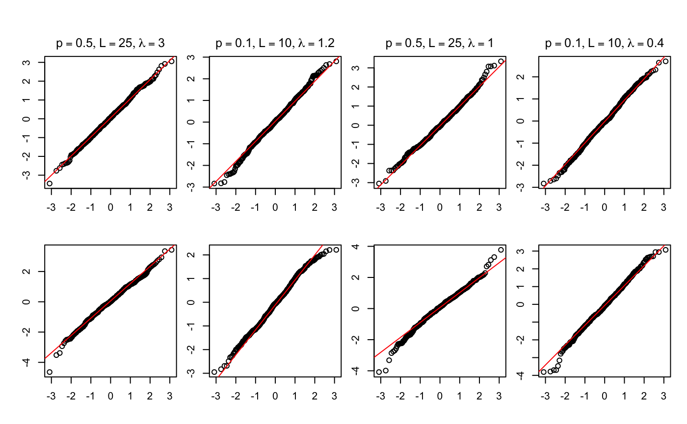
We generate by sampling with a random sign. For , it is generated uniformly from the hypersphere . In addition, entries of the covariate matrix are sampled independently from , and are normalized to have mean and scaled with . We choose from and adjust correspondingly. When , we choose and . When , we choose and . This results in combinations. For each setting, we generate the comparison graph and data times and record and . In Figures 1 and 2, we report the histograms and Q-Q plots of the following two normalized random variables:
respectively, where is defined in Theorem 3.1.
We conclude from Figures 1 and 2 that the empirical distributions of and follow closely the standard Gaussian distribution. These results validate our theoretical guarantee of normal approximation in Theorem 3.1 with the right asymptotic variance.

5.2 Goodness-of-Fit Test
In this section, we validate the theoretical guarantee of the goodness-of-fit test presented in Section 4.1 through a synthetic dataset.
We keep in the same way as those in the previous section. In order to set the signal strength at different levels, we generate and separately. Specifically, we first generate two vectors, and . The entries of are sampled independently from , while all entries of are fixed to be . We set at different signal levels as
where controls the signal strength. Additionally, and the covariate matrix are generated in a similar way as in the previous section.
The comparison graph and results are generated with and , and we fix . Applying the approach presented in Section 4.1 111we let and estimate the critical value using bootstraps. Given at each signal level, the comparison graph and data are generated for times to calculate the power function , we present the power functions in Figure 3. We conclude from Figure 3 that the Type I error is well controlled when the null hypothesis holds (). When the alternative holds, as the signal level increases, the power of the test increases rapidly, and the empirical probability reaches when . This demonstrates the efficacy of our proposed method for conducting the good-of-fit test.

5.3 Rank Confidence Interval
In this section, we study our out-of-sample ranking inferences application in Example 4.1 and the corresponding bootstrap theory from Theorem 4.2 in detail using synthetic data. We let , and let . For , we generate by sampling with a random sign. For and the covariate matrix, they are generated in a similar way as in the previous sections.
The comparison graph is generated with and . We are interested in six items with indices as representatives to validate our method, containing items from and items from . For each , we apply our method in Example 4.1 with . The regularized estimator is fitted with , and refitting with fixed support given by yields the two-stage estimator . We let , and the critical value is estimated by bootstrap samples.
The following Table 1 summarizes the experiment results, where for both one-step and two-step estimators, we report: (i). the empirical coverage of the rank confidence interval , (ii). the empirical coverage of the simultaneous confidence intervals (iii). the average length of the rank confidence interval, and the associated standard deviations. The empirical coverage proportion and the mean and standard deviation of the length are calculated from repeated experiments.
| One-stage | Two-stage | |||||
| item | Length | Length | ||||
| 1 | 0.96 | 27.61 2.97 | 1 | 0.94 | 13.0 1.51 | |
| 1 | 0.95 | 9.41 2.67 | 1 | 0.93 | 4.23 2.23 | |
| 1 | 0.97 | 14.06 2.44 | 1 | 0.94 | 8.35 2.05 | |
| 1 | 0.95 | 25.22 2.03 | 1 | 0.88 | 3.68 0.78 | |
| 1 | 0.98 | 38.95 4.01 | 1 | 0.89 | 6.03 0.96 | |
| 1 | 0.97 | 24.4 2.03 | 1 | 0.89 | 3.56 1.29 | |
5.4 Application to Pokemon Challenge Dataset
In this section, we apply our approaches to the Pokemon challenge dataset https://www.kaggle.com/c/intelygenz-pokemon-challenge/data. The dataset records pairwise competitions among pokemons. Each pokemon is accompanied by a set of covariate information, and each competition takes place between two pokemons and has one winner. We begin by utilizing our goodness-of-fit test in §4.1 to examine if covariates along can explain individual ability. Subsequently, we employ our predictive rank confidence interval approach to rank specific mega-evolved pokemon.
We assume that pokemons share the same intrinsic scores before and after mega evolution. Mega evolution only alters the covariates, thereby affecting the overall abilities of the pokemon. Consequently, it is natural to predict the abilities of mega-evolved pokemon using the combat results of their pre-evolutionary forms and their current covariates.
We randomly select mega evolved pokemons (out of a total of mega evolved pokemons) as our target. The remaining pokemons are left for training purpose. We constructed the comparison graph via the existing pairwise competitions. Since the graph was not connected, we selected the largest connected component as our training set to obtain a valid ranking result instead. Therefore, after this pre-processing step, we have pokemons left for training. For each pokemon, we consider a 3-dimensional covariates consisting of , and Mega or not. Attack and HP represent the ability to attack and durability, respectively, while Mega or not is a binary variable that denotes whether this pokemon is mega evolved or not.
As the first step, we conduct the goodness-of-fit test in §4.1 to verify the existence of non-zero intrinsic scores. We consider five values of the regularization parameter : and conduct the test for each . In Table 2, we report the test statistic , the critical value , as well as the estimated support size under each choice of . The critical value is estimated by bootstrapping samples. From Table 2 we can see that the null hypothesis is consistently rejected, and our approach is robust to the choice of regularization parameter . Note that in practice, one can choose via cross-validation.
Next, we apply our approach to construct out-of-sample rank confidence intervals for the mega evolved pokemons. We fix the regularization parameter and fit your model to get . Next, we refit our model with support constrained on the support of and obtain the two-stage estimator . For each of the mega evolved pokemons with index , we let pokemon with index be its pre-evolutionary version. If , the score of evolved pokemon is predicted as , otherwise, the score of pokemon is predicted as . On the other hand, we construct joint rank confidence interval with using the approach in §4.2. In Table 3 we show the rank of the predicted scores and the associated confidence intervals. We only present the results for pokemons whose IDs are multiples of as representatives. The results regarding the lengths of the confidence intervals are consistent with our conclusions from the simulation results.
| Pokemon ID | One-Stage method | Two-Stage method |
6 Conclusion
In this paper, we study entity ranking with covariates as well as sparse intrinsic scores. We introduce a novel model identification condition and derive the optimal statistical rates of the regularized maximum likelihood estimator (MLE). We further design a debiased estimator of the MLE and derive its asymptotic distribution. Our proposed method is further applied to studying the goodness-of-fit test of the model with no intrinsic scores, and we construct prediction confidence intervals for future latent scores as well their associated confidence intervals for ranks.
There are several directions for future research that are worth exploring. First, while we focus on a linear model in this paper, it would be valuable to investigate more complex models for explaining the latent scores in the future. Second, we consider only one evaluation criterion (i.e., only a fixed ) for all items. It would be interesting to incorporate heterogeneous evaluation criteria into the models. Third, it would be interesting to see how to combine our ranking framework with online or offline decision making tasks such as connecting with reinforcement learning with human feedback.
References
- Baltrunas et al. (2010) Baltrunas, L., Makcinskas, T. and Ricci, F. (2010). Group recommendations with rank aggregation and collaborative filtering. In Proceedings of the fourth ACM conference on Recommender systems.
- Berry (1941) Berry, A. C. (1941). The accuracy of the gaussian approximation to the sum of independent variates. Transactions of the american mathematical society, 49 122–136.
- Bradley and Terry (1952) Bradley, R. A. and Terry, M. E. (1952). Rank analysis of incomplete block designs: I. the method of paired comparisons. Biometrika, 39 324–345.
- Caron et al. (2014) Caron, F., Teh, Y. W. and Murphy, T. B. (2014). Bayesian nonparametric plackett–luce models for the analysis of preferences for college degree programmes.
- Chau et al. (2023) Chau, S. L., Cucuringu, M. and Sejdinovic, D. (2023). Spectral ranking with covariates. In Machine Learning and Knowledge Discovery in Databases: European Conference, ECML PKDD 2022, Grenoble, France, September 19–23, 2022, Proceedings, Part V. Springer.
- Chen et al. (2022a) Chen, P., Gao, C. and Zhang, A. Y. (2022a). Optimal full ranking from pairwise comparisons. The Annals of Statistics, 50 1775–1805.
- Chen et al. (2022b) Chen, P., Gao, C. and Zhang, A. Y. (2022b). Partial recovery for top-k ranking: Optimality of mle and suboptimality of the spectral method. The Annals of Statistics, 50 1618–1652.
- Chen et al. (2020) Chen, Y., Chi, Y., Fan, J., Ma, C. and Yan, Y. (2020). Noisy matrix completion: Understanding statistical guarantees for convex relaxation via nonconvex optimization. SIAM journal on optimization, 30 3098–3121.
- Chen et al. (2019) Chen, Y., Fan, J., Ma, C. and Wang, K. (2019). Spectral method and regularized mle are both optimal for top-k ranking. Annals of statistics, 47 2204.
- Chen and Suh (2015) Chen, Y. and Suh, C. (2015). Spectral mle: Top-k rank aggregation from pairwise comparisons. In International Conference on Machine Learning. PMLR.
- Chernozhukov et al. (2015) Chernozhukov, V., Chetverikov, D. and Kato, K. (2015). Comparison and anti-concentration bounds for maxima of gaussian random vectors. Probability Theory and Related Fields, 162 47–70.
- Chernozhuokov et al. (2022) Chernozhuokov, V., Chetverikov, D., Kato, K. and Koike, Y. (2022). Improved central limit theorem and bootstrap approximations in high dimensions. The Annals of Statistics, 50 2562–2586.
- Dwork et al. (2001) Dwork, C., Kumar, R., Naor, M. and Sivakumar, D. (2001). Rank aggregation methods for the web. In Proceedings of the 10th international conference on World Wide Web.
- Fan et al. (2022) Fan, J., Hou, J. and Yu, M. (2022). Uncertainty quantification of mle for entity ranking with covariates. arXiv preprint arXiv:2212.09961.
- Fan et al. (2020) Fan, J., Ke, Y. and Wang, K. (2020). Factor-adjusted regularized model selection. Journal of Econometrics, 216 71–85.
- Fan et al. (2023) Fan, J., Lou, Z., Wang, W. and Yu, M. (2023). Spectral ranking inferences based on general multiway comparisons. arXiv preprint arXiv:2308.02918.
- Fan et al. (2024) Fan, J., Lou, Z., Wang, W. and Yu, M. (2024). Ranking inferences based on the top choice of multiway comparisons. Journal of the American Statistical Association 1–28.
- Finch (2022) Finch, H. (2022). An introduction to the analysis of ranked response data. Practical Assessment, Research, and Evaluation, 27 7.
- Gao et al. (2023) Gao, C., Shen, Y. and Zhang, A. Y. (2023). Uncertainty quantification in the bradley–terry–luce model. Information and Inference: A Journal of the IMA, 12 1073–1140.
- Guo et al. (2018) Guo, Y., Tian, P., Kalpathy-Cramer, J., Ostmo, S., Campbell, J. P., Chiang, M. F., Erdogmus, D., Dy, J. G. and Ioannidis, S. (2018). Experimental design under the bradley-terry model. In IJCAI.
- Han and Xu (2023) Han, R. and Xu, Y. (2023). A unified analysis of likelihood-based estimators in the plackett–luce model. arXiv preprint arXiv:2306.02821.
- Han et al. (2020) Han, R., Ye, R., Tan, C. and Chen, K. (2020). Asymptotic theory of sparse bradley–terry model. The Annals of Applied Probability, 30 2491–2515.
- Li et al. (2019) Li, H., Simchi-Levi, D., Wu, M. X. and Zhu, W. (2019). Estimating and exploiting the impact of photo layout: A structural approach. Available at SSRN 3470877.
- Li et al. (2022) Li, X., Yi, D. and Liu, J. S. (2022). Bayesian analysis of rank data with covariates and heterogeneous rankers. Statistical Science, 37 1–23.
- Liu et al. (2022) Liu, Y., Fang, E. X. and Lu, J. (2022). Lagrangian inference for ranking problems. Operations Research.
- Luce (2005) Luce, R. D. (2005). Individual choice behavior: A theoretical analysis. Courier Corporation.
- Luce (2012) Luce, R. D. (2012). Individual choice behavior: A theoretical analysis. Courier Corporation.
- Ma et al. (2018) Ma, C., Wang, K., Chi, Y. and Chen, Y. (2018). Implicit regularization in nonconvex statistical estimation: Gradient descent converges linearly for phase retrieval and matrix completion. In International Conference on Machine Learning. PMLR.
- Massey (1997) Massey, K. (1997). Statistical models applied to the rating of sports teams. Bluefield College.
- Negahban et al. (2012) Negahban, S., Oh, S. and Shah, D. (2012). Iterative ranking from pair-wise comparisons. Advances in neural information processing systems, 25.
- Ouyang et al. (2022) Ouyang, L., Wu, J., Jiang, X., Almeida, D., Wainwright, C., Mishkin, P., Zhang, C., Agarwal, S., Slama, K., Ray, A. et al. (2022). Training language models to follow instructions with human feedback. Advances in neural information processing systems, 35 27730–27744.
- Plackett (1975) Plackett, R. L. (1975). The analysis of permutations. Journal of the Royal Statistical Society: Series C (Applied Statistics), 24 193–202.
- Raič (2019) Raič, M. (2019). A multivariate Berry–Esseen theorem with explicit constants. Bernoulli, 25 2824 – 2853.
- Rusmevichientong et al. (2010) Rusmevichientong, P., Shen, Z.-J. M. and Shmoys, D. B. (2010). Dynamic assortment optimization with a multinomial logit choice model and capacity constraint. Operations research, 58 1666–1680.
- Schäfer and Hüllermeier (2018) Schäfer, D. and Hüllermeier, E. (2018). Dyad ranking using plackett–luce models based on joint feature representations. Machine Learning, 107 903–941.
- Simons and Yao (1999) Simons, G. and Yao, Y.-C. (1999). Asymptotics when the number of parameters tends to infinity in the bradley-terry model for paired comparisons. The Annals of Statistics, 27 1041–1060.
- Stigler (1994) Stigler, S. M. (1994). Citation patterns in the journals of statistics and probability. Statistical Science 94–108.
- Talluri and Van Ryzin (2004) Talluri, K. and Van Ryzin, G. (2004). Revenue management under a general discrete choice model of consumer behavior. Management Science, 50 15–33.
- Tropp (2012) Tropp, J. A. (2012). User-friendly tail bounds for sums of random matrices. Foundations of computational mathematics, 12 389–434.
- Tropp (2015) Tropp, J. A. (2015). An introduction to matrix concentration inequalities. arXiv preprint arXiv:1501.01571.
- Turner and Firth (2012) Turner, H. and Firth, D. (2012). Bradley-terry models in r: the bradleyterry2 package. Journal of Statistical Software, 48 1–21.
- Zhao et al. (2022) Zhao, Z., Liu, A. and Xia, L. (2022). Learning mixtures of random utility models with features from incomplete preferences. arXiv preprint arXiv:2006.03869.
Appendix A Additional applications
We study the distribution of statistics
in order to construct one-sided rank confidence intervals. It’s distribution can be approximated by the bootstrap counterpart
We are able to achieve similar results as Theorem 4.2 for and . Next, we introduce some applications on constructing (simultaneous) one-sided confidence intervals for out-of-sample ranks via the distribution of in the following two examples.
Example A.1.
For an item of interest, and let be the targeted rank threshold, we are interested in the following testing problem
| (A.1) |
Let be the estimated -th quantile of from the bootstrap samples. As a result, by a similar analysis of Theorem 4.2, we have
Similarly, this implies
This yields a critical region at a significance level of for the test (A.1)
Appendix B Proof Outline of Estimation Results
B.1 Preliminaries and Basic Results
As the first step, let us look into the gradient and Hessian of the functions we are interested in. Except for and , we also define
The gradient of is controlled by the following lemma.
Lemma B.1.
With given by (2.5), the following event
happens with probability exceeding for some which only depend on .
Proof.
Let , its eigenvalues is studied in Fan et al. (2022, Lemma 15). We state it in the following lemma.
Lemma B.2.
Suppose for some . The following event
happens with probability exceeding when is large enough.
In the rest of the content, without loss of generality, we assume the conditions stated in Lemma B.2 hold. Moreover, with the help of Lemma B.2, we next analyze the Hessian and summarize its theoretical properties in Lemma B.3 and Lemma B.4, respectively.
Lemma B.3.
Suppose event holds, we obtain
Proof.
Since , we have
∎
Lemma B.4 can be viewed as the strong convexity property restricted on .
Lemma B.4.
Suppose event happens and . Then for all and such that , , we have
where .
Proof.
See §D.2 for a detailed proof. ∎
We then consider the following proximal gradient descent procedure. We set the step size and number of iterations .
Here we let and define
for any vector . Since is -strongly convex, the above proximal gradient descent enjoys exponential convergence. It is formalized in the following results.
Lemma B.5.
Under event , we have
where .
Proof.
See §D.3 for a detailed proof. ∎
Lemma B.6.
On the event happens, it follows that
Proof.
See §D.4 for a detailed proof. ∎
Lemma B.7.
On event , there exists some constant such that
Proof.
See §D.5 for a detailed proof. ∎
Next, we will leverage the leave-one-out technique and use induction to prove that the iterate stays close to the initial point during all the iterations .
B.2 Analysis of Leave-one-out Sequences
In this section, we construct the leave-one-out sequences (Ma et al., 2018; Chen et al., 2019, 2020) and bound the statistical error by induction. We consider the following loss function for any to construct the leave-one-out sequence.
Then for any , we construct the leave-one-out sequence in the way of Algorithm 2.
With the help of the leave-one-out sequences, we do induction to demonstrate that the iterate will not be far away from when With the leave-one-out sequences in hand, we prove the following bounds by induction for .
| (A) | ||||
| (B) | ||||
| (C) | ||||
| (D) |
For , since , the (A) (D) hold automatically. In the following lemmas, we prove the conclusions of (A)-(D) for the -th iteration are true when the results hold for the -th iteration.
Lemma B.8.
Proof.
See §D.6 for a detailed proof. ∎
Lemma B.9.
Proof.
See §D.7 for a detailed proof. ∎
Lemma B.10.
Proof.
See §D.8 for a detailed proof. ∎
Lemma B.11.
Proof.
See §D.9 for a detailed proof. ∎
Lemma B.12.
With probability exceeding we have
as long as .
Proof.
See §D.10 for a detailed proof. ∎
Appendix C Proof Outline of Uncertainty Quantification Results
Let be the quadratic expansion of the loss function around given by
| (C.1) |
Correspondingly, we define
First we state the following lemma for .
Lemma C.1.
For and defined in Eq. (2.5), as long as and for some constant , with probability at least , we have and
Proof.
See §D.12 for a detailed proof. ∎
With Lemma C.1 in hand, we control the difference then.
Theorem C.1.
For and defined in Eq. (2.5), as long as and for some constant , with probability at least , we have
Proof.
See §D.13 for a detailed proof. ∎
Next, we introduce the debiased version of and and prove the corresponding approximation results. Given a vector and a function , we define
With this definition, one can see that given any , we have
Take as an example first. From the derivative we know that
In other words, we can write
| (C.2) |
Therefore, we define the debiased estimator as
similar to we defined in (3.4). Then in the following content, we focus on controlling the difference . In order to do so, we construct an auxiliary function and consider its minimizer
| (C.3) |
Again, we define the debiased estimator as
Next, we control and separately.
Lemma C.2.
Under the conditions of Theorem C.1, with probability at least we have
Proof.
See §D.14 for a detailed proof. ∎
Lemma C.3.
Under the conditions of Theorem C.1, with probability at least we have
Proof.
See §D.15 for a detailed proof. ∎
From (C.2) we already know that
To get the asymptotic distribution of , we approximate by . The following lemma ensures the approximation error is small.
Lemma C.4.
Under the conditions of Theorem C.1, with probability at least we have
Proof.
See §D.16 for a detailed proof. ∎
Next, we consider the expansion of . Given a vector , a function and a vector , we define
Therefore, it is easy to see that
By the optimality condition we know that
Reorganizing the terms we get
where and . Inspired by this, we debias and as
| (C.4) |
In order to analyze the asymptotic distribution of
we approximate it by . The following lemma controls the approximation error.
Lemma C.5.
Under the conditions of Theorem C.1, with probability at least we have
Proof.
See §D.17 for a detailed proof. ∎
On the other hand, as long as is sufficiently small, the difference between and is also very small, which means that there is no need to debias . We have the following result.
Lemma C.6.
Under the conditions of Theorem C.1, with probability at least we have
Proof.
We combine the aforementioned results in this section and get the following expansion for and .
Theorem C.2.
Under the conditions of Theorem C.1, with probability at least we have
Proof.
See §D.18 for a detailed proof. ∎
C.1 Proof of the two-stage method in Section 3
We state the estimation error bounds for here. We define .
Lemma C.7.
Given and the aforementioned two stage estimator , as long as , with probability exceeding , we have
Proof.
We apply the Fan et al. (2020, Corollary A.1) directly. Let , by Lemma B.4 we know that the conditions in Fan et al. (2020, Corollary A.1) hold with . On the other hand, by Lemma D.1 we know that
As a result, as long as , we have
∎
We next approximate the estimator by the minimizer of the quadratic approximation of . Specifically, we define
with . As a result, it holds that
Then the following result controls the difference between and .
Proposition C.1.
Given and the aforementioned two-stage estimator , as long as , with probability exceeding , we have
Proof.
The optimality conditions tell us
Combine the above two equations together, we have
| (C.5) |
View as a sub-matrix of corresponding , similar to (D.29) we know that
| (C.6) |
On the other hand, again by the property of sub-matrix as well as Lemma B.4, we know that
| (C.7) |
Plugging (C.6) and (C.7) in (C.5) we get
As a result, we have
∎
C.1.1 Proof of Theorem 3.2
Proof.
We denote by . Then we can write
Consider the random vector
Then we have
By Berry-Esseen theorem we know that
| (C.8) |
Next, for any convex set with and point , we define
Therefore, we know that
| (C.9) |
Taking , by Theorem C.1 we know that
| (C.10) |
As a result, we know that
Plugging this as well as (C.10) in (C.9), we obtain
Since this holds for all convex , we know that
Similarly, we can also show that
Combine these two aforementioned inequalities with (C.8), it holds that
∎
Appendix D Proof of the Results
D.1 Proof of Proposition 2.1
Proof.
Assume we have two vectors such that
By (2.1) we know that
This tells us that we have for all . Consider the following index set
Since , we know that . Since , we pick different indices from . By the construction of we know that
for all . On the other hand, according to Assumption 2.1, we know that
As a result, we must that . This further implies
for all . This tells us that all the entries of are the same. And, since , we know that at least entries of are . As a result, we get . To sum up, we must have . ∎
D.2 Proof of Lemma B.4
D.3 Proof of Lemma B.5
Proof.
Since , we know that
As a result, we know that . As a result, we know that
| (D.3) |
Consider for . By the fundamental theorem of calculus we have
| (D.4) |
Let . By Lemma B.3 and the definition of we know that . Therefore, it holds that
| (D.5) |
Combine Eq. (D.3), Eq. (D.4) with Eq. (D.5), we know that
Therefore, under event , we have
∎
D.4 Proof of Lemma B.6
Proof.
Since is the minimizer, we have that . By the mean value theorem, for some between and , we have
As a result, we have
Therefore, we get
As a result, on event we have
We conclude the proof of Lemma B.6. ∎
D.5 Proof of Lemma B.7
D.6 Proof of Lemma B.8
Proof.
By definition we know that
By triangle inequality as well as the definition of SOFT we know that
| (D.6) |
Consider for . By the fundamental theorem of calculus, we have
Let be large enough such that
By the assumption of induction, we have
Then by Lemma B.4 as well as the induction assumption, we have
for all . On the other hand, by Lemma B.3, we have
Let , then it holds that
| (D.7) |
Therefore, plugging Eq.(D.6) in Eq. (D.7), and conditioned on event , we have
as long as and . ∎
D.7 Proof of Lemma B.9
Proof.
For any , by definition we have
This implies
| (D.8) |
We consider for . By the fundamental theorem of calculus we have
| (D.9) |
Consider which is large enough such that
Then we also have
Use the same approach when deriving Eq. (D.7), we have
| (D.10) |
as long as .
It remains to bound By definition, we have
By definition, we also have
Consider random variable . By Chernoff bound (Tropp, 2012), we know that
as long as for some . As long as , we have for . Since , by Hoeffding’s inequality and union bound, we get
with probability exceeding conditioning on as long as . On the other hand, since with probability exceeding , we have
with probability exceeding .
On the other hand, for we have
where
Consider . Since , we have that
By Bernstein inequality we know that
As a result, for we have
In summary, there exists constants which are independent of such that
| (D.11) |
with probability exceeding . Plugging Eq. (D.9), Eq. (D.10) and Eq. (D.11) in Eq. (D.8) we have
| (D.12) | ||||
| (D.13) |
as long as and is large enough such that .
∎
D.8 Proof of Lemma B.10
Proof.
For , we have
According to the induction assumption, we know that . As a result, we have
| (D.14) |
First, when , we have
| (D.15) |
Normalizing the numerators below to 1 and by the mean value theorem, there exists some between and such that
| (D.16) |
Combining Eq. (D.15) and Eq. (D.16), we have
By taking absolute value on both side, we get
Since , we have
By the defintion of we have
Consider which is large enough such that
Then we have
Then it holds that,
Using for , we have
Combine this result with Eq. (D.14), we get
| (D.17) |
as long as , and .
Second, let us focus on the case where . It suffices to control , which has been studied before. By Eq.(D.15), Eq.(D.16) as well as the fact that we know that
As a result, the left hand side can be controlled as
| (D.18) |
Again, since , we have . Plugging this in Eq.(D.18) and using the fact that , we get
| (D.19) |
As a result, as long as satisfies , we have
In this case, by Eq. (D.14) we know that . This as well as Eq. (D.17) tell us
Next we show . Let be any index which belongs to , it remains to show . By definition we know that
We write
According to the induction assumption, we have . This implies that . By triangle inequality we have
| (D.20) |
From Eq. (D.12) to Eq. (D.13) we know that
Combine this with Eq. (D.19) and Eq. (D.20) we have
Therefore, as long as is chosen such that
we have . In this case, we know that . In other words, . To sum up, it holds that
∎
D.9 Proof of Lemma B.11
Proof.
For any , we have
As a result, we have
as long as .
It remains to show that
For any , it suffices to show that . By definition we know that
We write
According to the induction assumption, we have . This implies that . By triangle inequality we have
| (D.21) |
Again, from Eq. (D.12) to Eq. (D.13) we have
Combine this with Eq. (D.19) and Eq. (D.21) we have
Since is already chosen to satisfy that
we have . In this case, we know that . In other words, . To sum up, it holds that
∎
D.10 Proof of Lemma B.12
Proof.
Since is the minimizer of , we know that
This implies . For any , we want to prove . It suffices to show that
For the same reason as Eq.(D.4) and Eq. (D.5), we know that
As a result, we can write
On the other hand, similar to Eq. (D.21) we know that
Combine this with Lemma B.7 we know that
As a result, as long as is chosen to satisfies
we have . In this case, we know that and thus . To sum up, we have
∎
Lemma D.1.
With given by 2.1, with probability at least we have
Proof.
For any , by definition we know that
Using Bernstein inequality conditioned on the comparison graph , with probability at least we have
The last holds since . As a result, we know that
with probability exceeding .
On the other hand, we write
Since , we have
| and |
Thus, with high probability (with respect to the randomness of ), we have
and
Let and . By matrix Bernstein inequality (Tropp, 2015), with probability at least we have
The last holds since . Therefore, we get
with probability exceeding .
∎
D.11 Auxiliary Lemma
Lemma D.2.
For , with probability at least we have
-
•
;
-
•
, , .
-
•
, for any .
Proof.
(1) By definition for we have
Since , by Bernstein inequality we have
with probability exceeding , as long as . On the other hand, since , we know that . As a result, we have
(2) By definition we have
with probability at least . Similarly, we have
and
with probability at least .
(3) For , by definition we know that is the average of independent Bernoulli random variables. By Hoeffding’s inequality, we know that
with probability at least . As a result, by union bound we know that
holds for all with probability at least . ∎
D.12 Proof of Lemma C.1
Proof.
We apply Fan et al. (2020, Theorem 4.1) to prove this statement. Use the notation in Fan et al. (2020), we denote by
We can see that Fan et al. (2020, Assumption 4.1) holds with and . Under our model, we have
As a result, the irrepresentable condition can be shown in the following way. By definition we have
| (D.22) |
Take in Lemma B.4, we know that
As a result, we have . On the other hand, Since the maximum in (D.22) is taken over , and , we know that
with probability at least . Plug these in (D.22), we get
As a result, as long as and for some constant , the irrepresentable condition Fan et al. (2020, Assumption 4.3) holds for (for defined in Fan et al. (2020)). According to Lemma D.1, since defined in Theorem 2.1 satisfies , by Fan et al. (2020, Assumption 4.1) we know that .
D.13 Proof of Theorem C.1
Proof.
By the strongly convex property we know that for any , we have
Since is the minimizer of , we know that . As a result, we know that
| (D.23) |
Similarly, for any , we have
Since and by the definition of we have
| (D.24) |
According to Theorem 2.1 and Lemma C.1, we know that and . Therefore, by Lemma B.4, (D.23) and (D.24) we know that
| (D.25) |
It remains to control the right hand side of the above inequality.
For any , we have
| (D.26) |
On the other hand, we also know that
| (D.27) |
(D.26) together with (D.27) implies
| (D.28) |
By the definition we can control the difference of hessian as
As a result, by Lemma B.2 we know that
| (D.29) |
with probability at least . Plugging (D.28) and (D.29) in (D.25) we get
According to Theorem 2.1 and Lemma C.1, the estimation error can be controlled as
∎
D.14 Proof of Lemma C.2
D.15 Proof of Lemma C.3
Proof.
Since is the minimizer of , we know that
for some real number between and . Reorganizing the terms gives
Combine this with the definition of (3.4) gives
Recall (D.30) that could be written as
As a result, the difference can be written as
| (D.31) |
We begin with controlling several terms in (D.31).
Control : By the definition we know that
with probability at least .
Control : By the definition we know that
with probability at least .
Control : By definition one can write that
| (D.32) |
where
On the other hand, by Taylor expansion we know that
where is some real number between and . As a result, we have
| (D.33) |
Plugging (D.32) in (D.33) gives us
Control : One can see that
with probability at least .
D.16 Proof of Lemma C.4
D.17 Proof of Lemma C.5
D.18 Proof of Theorem C.2
D.19 Proof of Theorem 3.1
Proof.
We begin with the asymptotic distribution of . We let . For such that and , we define
In this case, we have One can see that
conditioned on graph . On the other hand, since , we know that As a result, by Berry (1941) we have
Since with probability at least , we have
For simplicity we let
Consider event , where is some constant such that . Then for any fixed , we consider the following three events
Then we have
| (D.39) |
On the other hand, since , we know that
One can see that
Similarly, one can show that . Therefore, we have
Plugging this back to (D.39), and by the arbitrariness of , we have
Next we focus on the asymptotic distribution of . Similarly, we define
For such that and , we define
In this case, we have One can see that
conditioned on graph . On the other hand, since , we know that . As a result, by Berry (1941) we have
Since and , we know that
with probability at least (randomness comes from ). Similar to the discussion of before, one can further get
Then we mimic the proof of the counterpart again and one can show that
∎
D.20 Proof of Theorem 4.1
We define
and let be the -th quantile of conditioned on and . Let be a random vector such that is a Gaussian random vector and
Lemma D.3.
Proof.
Lemma D.4.
Under the conditions of Theorem 3.1, we have
Proof.
By definition of and we know that
Under the null hypothesis we have
| (D.40) |
According to (D.18), the first term on the right hand side of (D.40) can be bounded as
| (D.41) |
with probability at least . When it comes to the second term, by Lemma D.2 we have
| (D.42) |
with probability at least . And, one can see that
| (D.43) |
with probability at least . Plugging (D.41), (D.42) and (D.43) in (D.40) we get
with probability at least . As a result, we know that
| (D.44) |
with probability at least . We let
By Lemma D.3 we have
| (D.45) |
Therefore, by (D.44) and (D.45) we can write
| (D.46) |
By Chernozhukov et al. (2015, Theorem 3) the last term on the right hand side can be controlled as
Plugging this in (D.46) we get
∎
Lemma D.5.
Under the conditions of Theorem 3.1, we have
D.21 Proof of Theorem 4.2
Proof.
We define
where . Given , we define and . Let be a set of random variables such that is a set of joint Gaussian random variables and
We define
In the following proof, we let be any one of the three pairs: . Given , let be the -th quantile of . We are aiming at showing .
We start with the following lemmas.
Lemma D.6.
Under conditions of Theorem 2.1, we have
Proof.
By triangle inequality we have
On one hand, we know that
On the other hand, by definition we have
Therefore, we know that
∎
Lemma D.7.
Assume . Under the conditions of Theorem 3.1 and under the event , we have
Furthermore, we also have
Proof.
The Chernozhuokov et al. (2022, Condition E,M) holds with and . On one hand, we know that
On the other hand, since , by Lemma B.4 we know that
| (D.52) |
As a result, we know that
Therefore, by Chernozhuokov et al. (2022, Theorem 2.1, Theorem 2.2) we know that
∎
Lemma D.8.
Under the conditions of Theorem 3.1, as long as , we have
Proof.
By definition of and we know that
We write
| (D.53) |
According to (D.18), the first term on the right hand side of (D.53) can be bounded as
| (D.54) |
with probability at least . When it comes to the second term, by Lemma D.2 we have
| (D.55) |
with probability at least . And, by Lemma D.6 we have
| (D.56) |
with probability at least . Plugging (D.54), (D.55) and (D.56) in (D.53) we get
with probability at least . As a result, we know that
| (D.57) |
with probability at least . We let
By Lemma D.7 we have
| (D.58) |
Therefore, by (D.57) and (D.58) we can write
| (D.59) |
By Chernozhukov et al. (2015, Theorem 3) the last term on the right hand side can be controlled as
Plugging this in (D.59) we get
∎
Lemma D.9.
Under the conditions of Theorem 3.1, we have
