Functional Programming in Learning Electromagnetic Theory

Most physical situations are not exactly solvable. The traditional tools of algebra, calculus, and differential equations only get us so far. They can’t solve most problems. The theory tells you how to make (partial) differential equations, but you can’t solve them exactly. We don’t know how to write down functions that exactly satisfy the differential equations. Traditionally, you spend a lot of time studying situations that can be solved exactly, and then come up with tricks to approximate the other situations that can’t be solved exactly.

In EM theory, the electric field inside a capacitor with infinite plates is exactly solvable, but the electric field inside a capacitor with finite plates is not. The magnetic field produced by a circular loop carrying current is exactly solvable along the axis that runs through the center of the circle (perpendicular to the plane of the circle), but not exactly solvable anywhere else.

There are some simple, standard approximations (numerical methods), that are known to be reasonably good, and don’t involve tricks. The problem is that they require an enormous number of exceedingly boring computations. And here is where the computer comes to the rescue. Just by being able and willing to do an enormous number of simple, boring computations, the computer can give us good, approximate solutions to many problems.

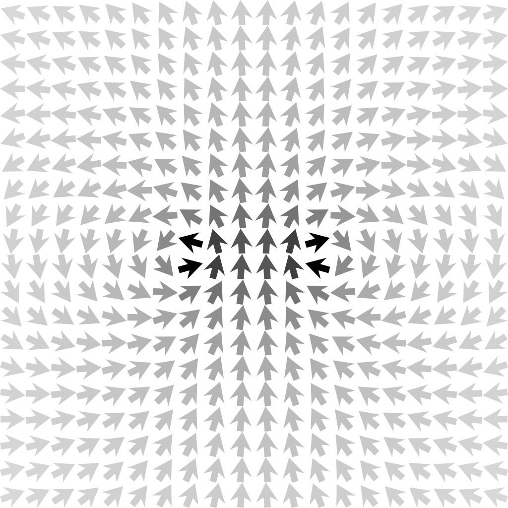
Figure 1 shows the numerically calculated magnetic field of a circular current loop, a problem which, surprisingly, is not analytically solvable.

Why not use all the tools at our disposal, and in particular the computer, to help us solve our problems? Computers can do things that calculators can’t. I don’t predict the death of the pocket calculator, but who knows? The slide rule is, if not dead, an eclectic tool used by very few people.

Physics societies like the American Association of Physics Teachers (AAPT) have been encouraging physics teachers to include more computer techniques in their courses.

Programming, like mathematics and like writing, is a valuable skill in itself. Knowing something about programming is useful for getting a job, but it’s also useful for organizing your thinking. (Mathematics and writing also help us organize our thinking.) Writing code is not just about getting the computer to do something. It’s also about expressing ideas using formal language in a way that makes sense to people. And so, for the same reason that essay writing can help you clarify your ideas about art or politics, code writing can help you clarify your ideas about physics.

In the preface to their wonderful book Structure and Interpretation of Classical Mechanics (SICM)[5], Sussman and Wisdom note

The traditional use of ambiguous notation is convenient in simple situations, but in more complicated situations it can be a serious handicap to clear reasoning. In order that the reasoning be clear and unambiguous, we have adopted a more precise mathematical notation. Our notation is functional and follows that of modern mathematical presentations.

and then

We require that our mathematical notations be explicit and precise enough that they can be interpreted automatically, as by a computer.

Sussman was the first pioneer in the application of functional programming to physics education. He showed the power of higher-order functions in physics using Scheme, a dialect of Lisp he co-invented with Steele, and used with Abelson in their classic computer science text Structure and Interpretation of Computer Programs[2].

The approach described in this paper is similar to SICM in that both are interested in using functional programming as a language for physics. Our approach differs from SICM in several ways. First, we use Haskell instead of Scheme, a difference which is noticeable primarily in our reliance on types and Haskell’s type system. Second, SICM is a graduate-level textbook while we target undergraduates. Third, SICM restricts its attention to classical mechanics, the theory of motion created by Newton and developed by Lagrange and Hamilton, while our concern in this paper is with a different theory of physics, namely electromagnetic theory.

The core of a pure functional programming language, while providing many interesting challenges for the compiler designer, presents a very simple model of computation to the user of the language. Names stand for values, not memory locations. Names refer to a single thing, and don’t change over time.

These are the principles upon which mathematical notation is based. Physics already uses mathematical language, so it is a smaller step for the physics student to learn the core of a pure functional programming language than it is to learn an imperative language. Obviously, there are trade-offs; functional programming’s affection for recursion can make teaching iteration more difficult.

In my courses, I teach students how to use the Haskell functions map, iterate, filter, take, and takeWhile as well as list comprehensions, but I do not teach them how to write explicitly recursive functions. Teaching recursion is a substantial endeavor, and I need to use the time to teach ideas of physics.

I have come to believe that a strong system of types is exceedingly helpful in a language for physics. Algebraic data types are useful in a language for physics for the same reason they are helpful in any domain-specific language, namely that the key ideas of the domain can be encoded as types.

The code writer can experience the benefits of clarity and organization of types even if she is not the person writing the data type definition.

An example of an algebraic data type in physics is charge distribution. Physicists like to talk about point charges, but they also like to talk about electric charge that is distributed along a curve, across a surface, or throughout a volume. A charge distribution is a specification of electric charge that could be at a point, along a curve, across a surface, throughout a volume, or some combination of these.

We use an algebraic data type to make charge distribution into a type.

data ChargeDistribution
    = PointCharge   Charge      Position
    | LineCharge    ScalarField Curve
    | SurfaceCharge ScalarField Surface
    | VolumeCharge  ScalarField Volume
    | MultipleCharges [ChargeDistribution]

The definition tells us that a charge distribution could be a point charge, a line charge (physicists use the term line charge for any one-dimensional distribution of charge; it need not occur along a straight line), a surface charge, a volume charge, or a combination of these. The ChargeDistribution data type is algebraic in having multiple constructors, and recursive in the last constructor.

We can see from its definition that the ChargeDistribution data type is based on other data types for physics like Charge, Position, ScalarField, Curve, Surface, and Volume. Charge is just a type synonym for double-precision floating point number. Position is a point in three-dimensional space. We’ll discuss the Position data type in the next section. Curve, Surface, and Volume are geometric objects that describe finite curves, surfaces, and volumes. These are helpful because EM theory has a substantial geometric content.

I do not demand that students be able to write algebraic data type definitions like this. Some students are interested in how this works, and I’m always happy to share what I know, but my main interest is in having students use this data type to describe a charge distribution. Using this data type brings one face to face with precisely what a charge distribution is, how we talk about it, and what’s it’s good for.

In EM theory, scalar and vector fields play a prominent role. A field in physics is a function of space or spacetime. In an undergraduate setting, it is more common to treat fields as functions of space, and I follow that custom with the following type synonyms for scalar field and vector field.

type ScalarField = Position -> R
type VectorField = Position -> Vec

In the first definition, R is a type synonym for Double, a double-precision floating point number. I like to think of these numbers as approximations to real numbers, and they occur so often in physics that it is convenient to give them a shorter name that comes closer to how we think about them. In the second definition, Vec is a data type for three-dimensional vectors. Such vectors are ubiquitous in physics, especially at the undergraduate pre-relativity level.

The central idea of electrostatics, the portion of EM theory focusing on electrical phenomena when nothing is changing in time, is that a charge distribution produces an electric field. We encode this central idea as a function.

eField :: ChargeDistribution -> VectorField

The type signature of eField sings the central idea of electrostatics. The definition of eField takes some effort to develop, as we need various kinds of integrals in order to deal with the continuous charge distributions. The type signature, however, serves as a wonderful summary and reminder of the big picture, and hopefully serves as a counterbalance to the possibility that people might get lost in the details of the function definition.

In fact, students routinely get lost in the traditional analytical presentation of electric field produced by a line charge, electric field produced by a surface charge, and electric field produced by a volume charge. There are so many details to worry about, and nothing in the traditional mathematical notation is reminding us of the central idea. A language with a strong system of types can help us keep the important ideas in mind.

Take the derivative from calculus as a higher-order idea that physics uses. The derivative of a function at a point expresses the rate at which the function changes at that point. We can write a numerical derivative in Haskell.

type R = Double

derivative :: R -> (R -> R) -> R -> R
derivative dt f t = (f (t + dt/2) - f (t - dt/2)) / dt

In this definition, dt is a numerical step size for the numerical derivative we are calculating. The second argument is the function f :: R -> R we want to differentiate. The third argument t :: R is the value of the independent variable where we want to estimate the slope.

Physicists like to think of the derivative as an “operator” that takes a function as input and gives another function as output. Haskell’s currying allows us to think just like that. Instead of thinking of the derivative as a function that takes three inputs (step size, function, and independent variable), we can think of derivative as a function that takes two inputs (step size and function) and returns a function. Even better, we can come to see that these two ways of thinking are the same for the computer because there is a sense in which there is no difference. The two ways of thinking are equivalent. Better yet, the function derivative 1e-6 really is the “operator” that takes a function as input and gives a function as output.

Numeric integration is another example of a higher-order function that encodes a basic idea of physics. And since calculus, vector calculus, and differential equations are so ubiquitous in physics, there are a plethora of higher-order functions serving calculus-related roles, some of which we will see later in this article.

Electromagnetic theory is primarily about vector fields, namely the electric and magnetic fields. We saw above that a vector field is a function, so any function that deals with a vector field is a higher-order function.

In physics, ideas we regard as basic, like the derivative, the integral, and the vector field, naturally invite us to use higher-order functions. Because higher-order functions in Haskell and other functional programming languages are easy to write and use, the language of the code can help you understand the theory. When a language allows a succinct expression of an idea that a domain regards as basic, using that language allows one to experiment and play with the idea, which is a great way to learn. Reading and writing in a language that makes it easy (or at least easier) to express the ideas in a theory promotes understanding of the theory. I claim that typed functional languages are especially suitable for physics, and I show examples below as evidence of this claim. I have anecdotal evidence that students understand analytical methods in electromagnetic theory better for having studied numerical methods in a functional programming language.

Physics has some results that can be obtained from deductive reasoning. The Maxwell equations imply conservation of electric charge, for example. In a course in EM theory, we show how to derive the continuity equation, an expression of local charge conservation, from the Maxwell equations.

This derivation takes a handful of steps, and although it doesn’t rise to the stature of a theorem as appreciated by mathematicians, nevertheless the language and pattern of a theorem are present. If the Maxwell equations are true, then the continuity equation is true. Such relationships are helpful to recognize, because a deep understanding of any theory requires going beyond “what is true” into knowing when ideas are independent, and knowing when one idea is a logical consequence of another.

Haskell, the language that I use in my EM theory class, is great for calculation, but not really intended for theorem proving. However, a handful of functional languages based on dependent types, such as Coq, Agda, Idris, and Lean, are capable of theorem proving (meaning proof checking with some automation) in addition to calculation.

It seems that a language that could calculate and prove would be a wonderful language in which to express the principles of physics. While I have great interest in this possibility, it is in no sense a reality in my teaching.

It seems to me that the possibility of using a dependently-typed functional language for physics in the future is a reason to learn a functional language like Haskell for physics now.

There are several ways of writing the Maxwell equations. Below we give a version known as the “integral form”. (There is also a “differential form” that is probably seen more often, but hides the geometric character of the theory.) For each of the four equations, I give a statement in words, followed by an equation in mathematical notation that expresses the same thing.

1. 1.

   Ampere-Maxwell Law: The rate of change of electric flux through a surface is the magnetic circulation around its boundary minus the current flowing through the surface.

   $$\frac{d}{dt}\int_{S}\vec{E}\cdot d\vec{a}=\frac{1}{\epsilon_{0}\mu_{0}}\int_{\partial S}\vec{B}\cdot d\vec{\ell}-\frac{1}{\epsilon_{0}}I$$

2. 2.

   Faraday’s Law: The rate of change of magnetic flux through a surface is the opposite of the electric circulation around its boundary.

   $$\frac{d}{dt}\int_{S}\vec{B}\cdot d\vec{a}=-\int_{\partial S}\vec{E}\cdot d\vec{\ell}$$

3. 3.

   Gauss’s Law: The electric flux through a closed surface is the charge contained inside.

   $$\int_{S}\vec{E}\cdot d\vec{a}=\frac{1}{\epsilon_{0}}Q$$

4. 4.

   No Magnetic Monopoles Law: The magnetic flux through a closed surface is zero.

   $$\int_{S}\vec{B}\cdot d\vec{a}=0$$

In these equations, $\vec{E}$ is the electric field and $\vec{B}$ is the magnetic field. Electric and magnetic fields are the fundamental physical quantities that electromagnetic theory deals with. They are created by charged particles, and they exert forces on charged particles. Most (perhaps all, I have no counterexample) physicists regard electric and magnetic fields to be just as real as the particles they interact with. Particles and fields, then, have a symbiotic relationship. Conceptually, they are equal partners in the explanation of electromagnetic phenomena, both dynamic actors on the electromagnetic stage. Most people, students included, have a much easier time imagining a particle than imagining a field. Electric and magnetic fields have type VectorField, which is a type synonym for Position -> Vec.

In the first two equations, $S$ is a surface and $\partial S$ is its boundary curve. An electric current $I$ flows through surface $S$. In the third and fourth equations, $S$ is a closed surface, containing some volume, and $Q$ is the total electric charge in that volume. The constants $\epsilon_{0}$ and $\mu_{0}$ appear in the equations because they use the International System (SI) of units. These constants are elided from the English-language descriptions.

Notice that surfaces and their boundary curves make an explicit appearance in this form of the Maxwell equations. This is evidence of the geometrical character of electromagnetic theory.

Beyond their role in the statement of the Maxwell equations, curves and surfaces are used to describe continuous charge and current distributions. We saw an example of this with the definition of the ChargeDistribution type in Section 2.6. The ChargeDistribution data type makes reference to the types Curve, Surface, and Volume. The simplest of these is the Curve data type, defined as follows.

data Curve = Curve { curveFunc          :: R -> Position
                   , startingCurveParam :: R  -- t_a
                   , endingCurveParam   :: R  -- t_b
                   }

A Curve is a map of one parameter into space, along with initial and final values of that parameter. A Surface is a map of two parameters into space, along with boundary data.

data Surface = Surface ((R, R) -> Position) R R (R -> R) (R -> R)

The first argument to Surface is the parameterizing function that maps $(s,t)$ into a Position. The second and third arguments are lower and upper limits of the parameter $s$. The fourth and fifth arguments are functions of $s$ that give the lower and upper limits of $t$. Allowing the limits of the second parameter to depend on the first parameter makes it easier to describe a surface like a triangle. The boundary of a Surface is a Curve.

A Volume is a map of three parameters into space, along with boundary information. The boundary of a Volume is a Surface.

Once we have data types for curves, surfaces, and volumes, vector calculus wants us to perform integrals over them.

For any vector field $\vec{F}$ and any surface $S$, the flux of the field through the surface is the integral

$$\int_{S}\vec{F}\cdot d\vec{a}.$$

The integral is calculated by approximating the surface $S$ by many small triangles. Each triangle has a vector area whose magnitude is the area of the triangle and whose direction is perpendicular to the triangle. At each triangle, we form the inner (dot) product of the vector field $\vec{F}$ at the location of the triangle and the vector area of the triangle; this inner product is a number. We add up these numbers for all of the triangles and call the result the flux of $\vec{F}$ through $S$. If the vector field is the electric field, we call the flux electric flux. If the vector field is the magnetic field, we call the flux magnetic flux. If $\vec{F}$ represented the flow of stuff, then the flux of $\vec{F}$ through $S$ is how much stuff flows through $S$.

Here is the Haskell code to approximate a flux integral.

dottedSurfaceIntegral :: SurfaceApprox -> VectorField -> Surface -> R
dottedSurfaceIntegral approx vF s
    = sum [vF r’ <.> da’ | (r’,da’) <- approx s]

The function dottedSurfaceIntegral needs an approximation method (type SurfaceApprox) to divide the surface into triangles.

type SurfaceApprox = Surface -> [(Position, Vec)]

This approximation method, called approx in the code, produces a list of pairs of positions and vector areas. The left side of the list comprehension shows that we take the dot product (using the operator <.>) of the vector field vF evaluated at position r’ with the vector area da’. The numerical results of the inner products are then added up with sum.

For any vector field $\vec{F}$ and any curve $C$, the circulation of the field along the curve is the integral

$$\int_{C}\vec{F}\cdot d\vec{\ell}.$$

The integral is calculated by approximating the surface $C$ by many small segments. Each segment has a vector length whose magnitude is the length of the segment and whose direction is along the segment. At each segment, we form the inner (dot) product of the vector field $\vec{F}$ at the location of the segment and the vector length of the segment; this inner product is a number. We add up these numbers for all of the segments and call the result the circulation of $\vec{F}$ along $C$. If the vector field is the electric field, we call the circulation electric circulation. If the vector field is the magnetic field, we call the circulation magnetic circulation.

Here is the Haskell code to approximate a circulation integral.

dottedLineIntegral :: CurveApprox -> VectorField -> Curve -> R
dottedLineIntegral approx f c = sum [f r’ <.> dl’ | (r’,dl’) <- approx c]

The function dottedLineIntegral needs an approximation method to divide the curve into segments. This approximation method, called approx in the code, produces a list of pairs of positions and vector lengths. The left side of the list comprehension shows that we take the dot product (using the operator <.>) of the vector field f evaluated at position r’ with the vector length dl’. The numerical results of the inner products are then added up with sum.

There are quite a number of these line, surface, and volume integrals that are used in electromagnetic theory. The table below shows the nine integrals that EM theory needs from vector calculus.

Haskell function	mathematical notation	requires
scalarLineIntegral	$\int_{C}f\ d\ell$	scalar field	curve
vectorLineIntegral	$\int_{C}\vec{F}\ d\ell$	vector field	curve
dottedLineIntegral	$\int_{C}\vec{F}\cdot d\vec{\ell}$	vector field	curve
crossedLineIntegral	$\int_{C}\vec{F}\times d\vec{\ell}$	vector field	curve
scalarSurfaceIntegral	$\int_{S}f\ da$	scalar field	surface
vectorSurfaceIntegral	$\int_{S}\vec{F}\ da$	vector field	surface
dottedSurfaceIntegral	$\int_{S}\vec{F}\cdot d\vec{a}$	vector field	surface
scalarVolumeIntegral	$\int_{V}f\ dv$	scalar field	volume
vectorVolumeIntegral	$\int_{V}\vec{F}\ dv$	vector field	volume

Vector calculus has its own versions of the fundamental theorem of calculus, the theorem that makes precise the idea that derivatives and integrals are inverse operations of each other. The fundamental theorems of vector calculus are known as the gradient theorem, Stokes’ theorem, and the divergence theorem. They can be expressed using the integrals in the table above.

After students understand the meaning of the integrals in the table above, they are in a position to study the three fundamental theorems of vector calculus. Since each theorem claims that an integral of a derivative over some geometric object is equal to a different integral over the boundary of that object, checking these fundamental theorems provides opportunities to practice evaluating the integrals. Even better, the two sides, which are each a bit of a challenge to set up, must give the same number in the end, which serves as satisfying evidence that the integrals were done correctly.

Stokes’ theorem claims that for any vector field $\vec{F}$ and any surface $S$, the following equality holds.

$$\int_{S}(\vec{\nabla}\times\vec{F})\cdot d\vec{a}=\int_{\partial S}\vec{F}\cdot d\vec{\ell}$$

The expression $\vec{\nabla}\times\vec{F}$ is called the curl of $\vec{F}$. The curl is a vector derivative that takes a VectorField as input and produces a VectorField as output. The physical meaning of the curl is the extent to which a vector field, if it were a velocity field of water, encourages rotation of a small object placed in the water. A vector field with zero curl is called conservative, meaning that a dotted line integral of the field around any closed curve is zero.

The following homework problem, which was assigned in fall 2023, asks students to check Stokes’ theorem for a particular vector field and a particular surface.

Homework Problem: Check Stokes’ theorem using the vector field

$$\vec{F}(x,y,z)=-z\hat{y}+y\hat{z}$$

and the rectangular region with corners $(x,y,z)=(0,0,-4)$, $(0,2,-4)$, $(0,2,4)$, $(0,0,4)$, in which the orientation is in the positive $x$ direction.

Checking the fundamental theorem for curls means (a) finding the curl of your vector field, (b) finding the flux integral of the curl over the surface, (c) finding the line integral (the circulation) of your vector field over the boundary of the surface (which has 4 parts), and (d) confirming that the results from (b) and (c) are the same. You may do this problem analytically, numerically, or a combination of both.

To solve this homework problem numerically with Haskell, we first encode the vector field $\vec{F}$ as vF and the rectangle as rect.

vF :: VectorField
vF r = let (x,y,z) = cartesianCoordinates r
       in (-z) *^ yHat r ^+^ y *^ zHat r

rect :: Surface
rect = Surface (\(y,z) -> cart 0 y z) 0 2 (const (-4)) (const 4)

To calculate the left-hand side of Stokes’ theorem, we need to take the curl of the vector field. As with a numerical derivative, we need to give a step size over which to evaluate the curl; we choose $10^{-6}$.

curlF :: VectorField
curlF = curl 1e-6 vF

Now we can calculate the left side of Stokes’s theorem.

leftSide :: R
leftSide = dottedSurfaceIntegral (surfaceSample 200) curlF rect

We get the result 32.00000000236293. For the right side, we need the boundary curve of the reactangle.

boundaryParam :: R -> Position
boundaryParam t
    | t < 1      = cart 0 (2*t) (-4)
    | t < 2      = cart 0 2 (8*(t-1) - 4)
    | t < 3      = cart 0 (2 - 2 * (t-2)) 4
    | otherwise  = cart 0 0 (4 - 8 * (t-3))

boundaryOfRect :: Curve
boundaryOfRect = Curve boundaryParam 0 4

rightSide :: R
rightSide = dottedLineIntegral (curveSample 1000) vF boundaryOfRect

The right side gives 32.0, which is reasonably close to the left side, and can be explained by numerical error.

In this homework problem, I give students the choice about whether to use analytic (pencil and paper) methods, numerical methods, or a combination of both. I do not always give students this choice. Sometimes I demand they use analytic methods; sometimes I demand they use numerical methods. At least one third of the time, however, I give students the choice, which they seem to appreciate.

For this homework problem in fall 2023, 5 of the 10 students who submitted it chose to do it analytically, and 5 chose to do it numerically using Haskell.

As a last example of the power of types and higher order functions in EM theory, we turn to calculation of the magnetic field by the Biot-Savart law.

References

- [1]
- [2] Harold Abelson, Gerald Jay Sussman & Julie Sussman (1996): Structure and Interpretation of Computer Programs, second edition. MIT Press.
- [3] David J. Griffiths (2017): Introduction to Electrodynamics. Cambridge University Press, 10.1017/9781108333511.
- [4] Seymour A. Papert (1993): Mindstorms: Children, Computers, And Powerful Ideas, 2 edition. Basic Books.
- [5] Gerald Jay Sussman & Jack Wisdom (2001): Structure and Interpretation of Classical Mechanics. The MIT Press.
- [6] Gerald Jay Sussman & Jack Wisdom (2013): Functional Differential Geometry. The MIT Press.
- [7] Scott N. Walck (2014): Learn Physics by Programming in Haskell. In James Caldwell, Philip Hölzenspies & Peter Achten, editors: Proceedings 3rd International Workshop on Trends in Functional Programming in Education, Soesterberg, The Netherlands, 25th May 2014, Electronic Proceedings in Theoretical Computer Science 170, Open Publishing Association, pp. 67–77, 10.4204/EPTCS.170.5.
- [8] Scott N. Walck (2016): Learn Quantum Mechanics with Haskell. In Johan Jeuring & Jay McCarthy, editors: Proceedings of the 4th and 5th International Workshop on Trends in Functional Programming in Education, Sophia-Antipolis, France and University of Maryland College Park, USA, 2nd June 2015 and 7th June 2016, Electronic Proceedings in Theoretical Computer Science 230, Open Publishing Association, pp. 31–46, 10.4204/EPTCS.230.3.
- [9] Scott N. Walck (2023): Learn Physics with Functional Programming: A Hands-on Guide to Exploring Physics with Haskell. No Starch Press.
- [10] Brent Yorgey (2011–2016): The diagrams package. https://hackage.haskell.org/package/diagrams.