Probing Dark Energy Evolution Post-DESI 2024
Abstract
We study the evidence for dark energy (DE) evolution at low redshift, using baryonic acoustic oscillations (BAOs) from the DESI Early Data Release, Pantheon+ Type Ia supernovae (SNe-Ia), and redshift space distortions (RSDs) to constrain cosmological parameters. Furthermore, we make use of the angular acoustic scale to analyse the effect of introducing condensed CMB information on the cosmological parameters informing DE evolution. The analysis is divided into cases based on the variability of priors inferred from early-time physics. Using a quadratic parametrisation, , for DE density, we find evidence for DE evolution in all cases, both with and without the angular acoustic scale. We reconstruct using best fit parameters and find that DE density starts to exhibit dynamical behaviour at , assuming negative values beyond . The data show no significant preference for CDM over a CDM, with both models performing equally well according to our chosen metrics of reduced and the Durbin-Watson statistic.
I Introduction
The Early Data Release from the Dark Energy Spectroscopic Instrument (DESI, [1, 2, 3]) has motivated further exploration of dynamical dark energy (DE) in place of a cosmological constant in the standard cosmological model, CDM [4, 5, 6, 7, 8, 9, 10, 11, 12, 13]. Prominant CDM alternatives include quintessence models [14, 15, 16, 17, 18, 19] and theories of modified gravity [20, 21, 22, 23, 24, 25, 26], many of which have been revised in light of the recent DESI data release [4]. The most common approach to look for potential deviations from the CDM model is to represent the DE component using the equation of state parameter . This approach assumes there is an unknown component with energy density given by
| (1) |
This approach, in principle, admits a phantom behavior (), but does not allow the excursion to negative DE densities. However, the authors of [27, 28], demonstrate that the method is inherently constrained because the functions that connect observations with theory, such as the luminosity distance, rely on through a complex integral relationship. This obscures detailed information about and its temporal changes, reducing the precision with which can be determined from existing data.
Rather than initially adopting a particular physical model for DE, given our lack of clear insight into its origin, in this work we opt for an exploratory approach, utilizing a probing function to represent the DE density. Our aim is to identify deviations from the CDM model which assumes a constant DE component. This approach started in [29, 30, 31], where the authors used both a linear and a quadratic probe function for . For CDM, , whilst if for any redshift , this is an indication of DE evolution. In [32] it was found that low redshift observational data prefer that decreases with , even taking negative values for . The same trend has been found using new data, such as the Pantheon+ sample [33, 34], and also using new methods, such as non-parametric and even biology inspired ones, discussed in [34, 35]. This trend of including the possibility of a negative is a challenge for DE modeling.
The paper is organised as follows. The next section introduces the methodology and datasets used for the statistical analysis. The main results are described in section III. We make our concluding remarks in section IV.
II Methodology and data
Assuming an isotropic, homogeneous universe, characterised by a flat FLRW spacetime metric, the Hubble parameter is defined as follows,
| (2) |
where the energy densities parameters of matter, radiation, and dark energy are described by , , and , respectively. We restrict our analysis to the flat case, thus, . Whilst is a constant to be constrained directly, we make use of the relation,
| (3) |
for in our analysis of BAO data [36]. is effective number of neutrinos, is photon energy density, and is neutrino energy density.
We adopt an agnostic approach in attempting to describe the behaviour of dark energy, parametrising DE density as a second degree polynomial,
| (4) |
This parametrisation is a continuation of the work in [33, 32, 34]. Variables and are constant values of evaluated at , and , where . Using the same definitions as in [33], , , , where is the maximum redshift value across the three datasets used in this analysis. The free parameters in then become and . These definitions reduce (4) to
| (5) |
The first thing to note is the concordance between this cosmological model, which we shall refer to as CDM, and CDM, in the case of no DE evolution. If the data prefer constant over dynamical DE density, then and will tend to unity, reducing (5) to the CDM model. CDM, therefore, may be thought of as an extension of the mostly successful CDM model, in pursuit of exploring the possibility of dynamical DE at low redshift.
The model is put under stress using four types of observational data: baryonic acoustic oscillation data from DESI [1], Type Ia supernovae from the Pantheon+ sample [37], redshift space distortions from a sample compiled by the authors of [38], and cosmic microwave background radiation data from the acoustic angular scale, also used in [1].
II.1 Baryonic Acoustic Oscillations
The first dataset we use to extract cosmological parameters is DESI’s first year release of baryonic acoustic oscillations (BAOs) [1]. The dataset consists of 12 points, with redshift () ranging from 0.295 to 2.330. There are five redshift values at which both the transverse (/) and radial (/) components of BAOs are reported, and two redshifts at which only the an angle-averaged distance, /, is reported.
The theoretical values for these BAO measurements are obtained using the following relations, where the drag-epoch sound horizon:
| (6) |
in the radial direction,
| (7) |
in the transverse direction, and
| (8) |
for the angle-averaged distance, calculated instead for the two data points with a significantly low signal-to-noise ratio [2].
To constrain the parameters of a given cosmological model using BAO data, we require prior knowledge of a sort to break the degeneracy between and . In [1] this was achieved in two ways, the first of which makes use of CMB [39] and CMB lensing [40, 41, 42, 43] information to directly calibrate , such that Mpc is fixed. The second method involves introducing a Big Bang Nucleosynthesis (BBN)-inferred prior on , followed by use of the early-time physics approximation for the drag-epoch sound horizon [44].
We opt for a different approach to the - degeneracy problem that allows for an explicit dependence on the parameters of a given cosmological model in the determination of . This approach is similar to the second method outlined above, however, instead of using an approximate equation for , we used the integral definition to calculate the drag-epoch sound horizon,
| (9) |
where is redshift at the drag-epoch, and , the speed of sound, is given by
| (10) |
In this way, is treated as another theoretical function, defined in terms of cosmological parameters, to be fitted to data.
It should be noted that the adoption of in integral form alone is not sufficient to overcome - degeneracy and determine the remaining cosmological parameters. The integral approach is also dependent on prior knowledge, specifically, the calculation of involves , , where , and . We examine the impact on our results of assuming such values to be fixed, versus allowing them to be free variables within the equation for . When fixed, the variables assume values of (standard model prediction [45, 46]), [47], and [48].
In the case of , , and as free variables, we introduce Gaussian priors on all three variables. The prior on is BBN-inferred [47], and the prior on is a Gaussian constructed around a mean of value 1059, with standard deviation 10– a conservative estimate. The authors of [1] also consider varying in their analysis. Combining CMB and CMB lensing information from Planck [39] and the Atacama Cosmology Telescope (ACT) [41, 43, 42] with DESI BAO data, they report a value of . We use this result for our prior.
Allowing these parameters to vary serves primarily as an exercise in agnosticism. The fixed values for all three variables are derived using CDM, introducing a dependence on the very model we aim to explore deviations from (albeit deviations at low redshift). Whilst we expect that an alternative cosmological model will agree with the results of CDM at early times, it is nonetheless interesting to explore the implications of allowing , , and to become free variables.
II.2 Type Ia Supernovae
The second and largest dataset used in our analysis is the Pantheon+ Type Ia SNe (SNe-Ia) sample, consisting of 1701 observed magnitude measurements at redshifts ranging from 0.00122 to 2.26137 [37]. Of these data, 77 data points are calibrated using Cepheid variables, and the remaining 1624 points are left uncalibrated. Making use of the luminosity distance equation,
| (11) |
with explicit dependence on the Hubble parameter, allows for theoretical apparent magnitude to be expressed as follows,
| (12) |
where is the absolute magnitude of SNe-Ia. Best fit values for the cosmological parameters in may be fitted to SNe-Ia data by comparing apparent magnitude predictions from (12) with the Pantheon+ results. Since the SNe-Ia sample is used in combination with BAO data throughout this analysis, we omit the use of a standard candle-inferred prior on , such as the Riess prior (R21) of km s-1 Mpc-1 [49]. At no point in this analysis is subject to priors of any kind, in tandem with the motivation for seeking a model beyond CDM: uncertainty around the true value of .
II.3 Redshift Space Distortions
The third data included in this analysis are 63 growth rate parameter values () from redshift space distortions (RSDs) at redshifts ranging from 0.001 to 1.944. This dataset is an amalgamation of RSD data collected between 2006 and 2008, and was first constructed by the authors of [38] in their analysis of the tension. This tension can also be related to the tension, from weak lensing measurements, viewed in the plane , where . Weak lensing measurements from three galaxy surveys, the Dark Energy Survey (DES), Kilo-Degree Survey (KiDS), and Hyper Suprime-Cam Subaru Strategic Program (HSC SSP), have yielded consistent results, revealing a tension with Planck [50, 51, 52].
The following second-order ordinary differential equation describes the evolution of density perturbations,
| (13) |
where is the normalized Hubble parameter as a function of the scale factor (). In a similar manner to the authors of [38], we solve this ODE numerically for to generate a function for [53] in terms of cosmological parameters used in the analysis of BAO and SNe-Ia data.
This sample, however, lacks the accuracy of the previous two datasets due to significantly larger errors associated with the measurements. Thus, whilst alone it has a limited ability to precisely determine cosmological parameters, in conjunction with the other two datasets, the RSD data serve both to constrain the model further, and as a consistency check for our results that do not involve RSDs.
As the authors of [38] highlight, smaller RSD samples are typically seen in cosmological analyses, works [54, 55, 56, 57, 58, 59, 60, 61, 62, 63, 64, 65, 66, 67, 68] being examples from prior to the publication of [38]. More recently, this still holds true in papers exploring CDM alternatives using combinations of BAO, SNe-Ia, and RSD data [69, 70, 71, 72, 73], with a reluctance to use all available RSD datasets in aggregate due to correlated data points. Since the total available RSD data lack a full covariance matrix to account for these correlations, the authors of [38] introduce "a nontrivial covariance matrix correlating randomly 20 of the RSD data points." They report that this has no significant effect on the main results of their analysis, hence, we proceed with the full dataset (see Table II of [38]).
It is worth noting a difference in parametrisation of in the analysis of BAO and RSD data. In the calculation of from (9), it is necessary to account for the radiation contribution to (3) as a distinct entity, in alignment with early-time physics. Alternatively, in our analysis of the late-time RSD data, we treat as negligible.
II.4 Acoustic Angular Scale
The final constraint imposed on the parameters of each cosmological model is the CMB-inferred acoustic angular scale from Planck [39]. We incorporate this condensed CMB information into our analysis in the same manner as the authors of [1]. The acoustic angular scale, , is given by , where
| (14) |
and is the redshift at the epoch of recombination [39]. may be interpreted geometrically as "the BAO scale imprinted in the CMB anisotropies at recombination," [1]. As such, introducing condenses CMB-realised information about the early universe into a constraint on the late-time () data from DESI, Pantheon+, and RSDs. Whilst the Planck value of makes use of the CDM model in its derivation, here we invoke our assumption that CDM alternatives ought to agree with CDM at early times. We leave as a function of cosmological model parameters with a Planck-inferred Gaussian prior of mean and standard deviation as cited above.
| Parameter | Prior |
|---|---|
II.5 Calculating and Durbin-Watson
For both CDM and CDM, we report best fit cosmological parameters for the combinations of DESI, Pantheon+, and RSD data, with and without (see Table 2(a)). Below is outlined our method for the calculation of reduced chi-squared () and the Durbin-Watson (DW) statistic, measures of goodness of fit.
Considering the DESI sample alone, the 10 data points for which either or is reported have associated covariance matrices (). We use
| (15) |
where is the vector (, ) and is its theoretical counterpart, to calculate the contribution of these data to the final DESI chi-squared statistic, . For the remaining two data points, is reported with an uncertainty value, . We use
| (16) |
to estimate their contribution to . Thus, for the entire BAO sample, we have .
For Pantheon+, is computed using
| (17) |
where is the associated covariance matrix. The components of vector are given by for the 1624 uncalibrated data points, and for the remaining 77 apparent magnitude values calibrated using Cepheid variables.
For the RSD data,
| (18) |
We weight each sample’s contribution to the final chi-squared statistic evenly, such that
| (19) |
With the inclusion of ,
| (20) |
where assumes the mean and standard deviation of ) as the measured value (see Table 1). In the cases where , and are variable, their associated Gaussian priors (see Table 1) are also added explicitly to .
To obtain the reduced statistic, we use
| (21) |
where the number of degrees of freedom, , is assumed equal to for data points and parameters [74]. We treat as a single data point in its contribution to .
The DW statistic is given by
| (22) |
where is the residual for a given data point; where is the data point and is the corresponding model value. For a large number data points, the statistic is equal to , where is the autocorrelation of the residuals. If no correlation is found, we expect . implies is evidence for positive correlation, and for negative correlation. We use the Python module statsmodels [75] to compute the statistic.
II.6 Markov Chain Monte Carlo (MCMC) Sampling
We make use of the public code emcee [76] for MCMC sampling. As outlined in [35], the Metropolis-Hastings algorithm is invoked to attain the posterior for the relevant cosmological parameters from the likelihood function and prior distribution of parameters. We minimize using the Nelder-Mead method to decipher a starting position within the parameter space, before walkers are set off for 5000 steps. The first 20 samples are neglected as burn in. We use GetDist [77] to visualise the triangle plots for the resulting posterior distributions.
III Results
| DW | ||||||||
|---|---|---|---|---|---|---|---|---|
| Flat CDM | ||||||||
| DESI+Panth.+RSD | – | – | 0.895 | 1.68 | ||||
| DESI+Panth.+RSD+ | – | – | 0.902 | 1.70 | ||||
| Flat CDM | ||||||||
| DESI+Panth.+RSD | 0.886 | 1.72 | ||||||
| DESI+Panth.+RSD+ | 1.14 | 1.74 |
| DW | ||||||||
|---|---|---|---|---|---|---|---|---|
| Flat CDM | ||||||||
| DESI+Panth.+RSD | – | – | 0.893 | 1.69 | ||||
| DESI+Panth.+RSD+ | – | – | 1.19 | 1.71 | ||||
| Flat CDM | ||||||||
| DESI+Panth.+RSD | 0.887 | 1.72 | ||||||
| DESI+Panth.+RSD+ | 1.11 | 1.74 |
| DW | ||||||||
|---|---|---|---|---|---|---|---|---|
| Flat CDM | ||||||||
| DESI+Panth.+RSD | – | – | 0.893 | 1.70 | ||||
| DESI+Panth.+RSD+ | – | – | 1.12 | 1.71 | ||||
| Flat CDM | ||||||||
| DESI+Panth.+RSD | 0.889 | 1.72 | ||||||
| DESI+Panth.+RSD+ | 1.17 | 1.74 |
Tables 2(a), 2(b), and 2(c) summarise the results of MCMC sampling in the three different cases with varying constraints on , , and . We begin the analysis of our results by discussing the goodness of fit of both cosmological models. We proceed to analyse the effect of varying , , and on the resulting cosmological parameters for both models. We compare CDM and CDM values for and with previous analyses. Finally, we reconstruct and , the deceleration parameter, using best fit parameters, and explore the implications for DE evolution.
In our evaluation of goodness of fit we make use of two statistics: and Durbin-Watson (DW). The combination allows for a more robust analysis, as the two statistics assess different qualities of a given model. The DW statistic tests for serial autocorrelations of the residuals, a characteristic that cannot account for [78], with a desired value of 2. The more familiar statistic within the field of cosmology, , has an ideal value of 1, with lower values implying over-fitting [74].
The statistics in Table 2(a), when considered in aggregate, imply no significant preference for CDM over CDM. For the combination of all three datasets with , the and DW values for CDM are 1.14 and 1.74, respectively. In the same case, for CDM, and DW . The proximity of the and DW values to their desired values of 1 and 2, respectively, indicates successful data-fitting from both models. The case outlined above is the most constrained (fewest free parameters) and hence, shall be a focal point in our analysis. However, the success of CDM being comparable to that of CDM extends to all cases. Furthermore, the DW statistic favours CDM universally. It should also be highlighted that all and DW values across the three tables remain acceptably close to the desired values. In this way, both models are competitive in describing the observational data used, both fitting the data and obtaining a small autocorrelation. Hence, neither model should be outright rejected.
By a comparison of the results in Tables 2(a), 2(b), and 2(c) we observe – as expected – that increasing the number of free parameters increases the resulting best fit value for in the case of CDM: DESI+Panth.+RSD+. We find that for , , and fixed lies lower than for , , and all variable. We define , where and are the mean uncertainty values associated with the given results. This implies that increased uncertainty in early-time physics variables and, hence, fewer assumptions in our CDM model, does impact best-fit cosmological parameters, specifically increasing . We note that in both cases with variable (Tables 2(c) and 2(b)), a consequence of this variability is increasing to , a deviation from the prior distribution mean. This increase in cosmological parameters is not observed in the corresponding CDM results to a significant degree.
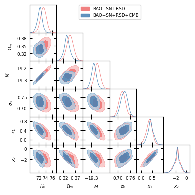
To comment briefly on , across Tables 2(a), 2(b), and 2(c), we observe lower values in the CDM analyses than those of CDM both with and without . Including , the CDM value of in 2(a) differs from the 2018 reported Planck value of at the 4.7 level.
To compare an CDM value of with those from other analyses, we confine the rest of our discussion to the results in Table 2(a), reflecting the analysis with the fewest free variables.
First, we consider the results of our analyses excluding . For CDM, we report km/s/Mpc, with free parameters and . The corresponding CDM results are km/s/Mpc, a deviation of from the CDM case.
The addition of lowers universally, as expected, giving rise to a larger discrepancy of between the two models. In the CDM case, km/s/Mpc, with and . Even with the addition of condensed CMB information, remains significantly closer to the Cepheid-SNe-Ia deduced value of km/s/Mpc [49], differing by only . When compared with the Planck value of km/s/Mpc [39], a much larger discrepancy of arises, confirming that the CDM model fails to resolve the Hubble tension when constrained by these three datasets and the angular acoustic scale. An interesting extension of this work would be to incorporate additional CMB information beyond from Planck and the ACT to be used in combination with BAO, SNe-Ia, and RSD data.

Despite CDM’s failure at resolving the Hubble tension, the model may still offer some insight into the nature of DE at low redshift. More specifically, in all CDM cases, the data prefer and . Both parameters showing significant deviation from unity is suggestive of dynamical DE at low redshift. Using the best fit parameters for in Table 2(a), DE density is re-parametrised and plotted as a function of redshift (), as shown in Fig. 2. As increases beyond , DE density begins to exhibit dynamical behaviour and decays quadratically, assuming negative values beyond . DE density decreasing beyond zero is supported at the 2 above the best fit curve.
At low redshift, , , in agreement with CDM, although this feature of the reconstruction should be interpreted with caution. A quadratic parametrisation lacks the ability to detect fluctuations at low redshifts– it is constrained by the properties of a second degree polynomial. The authors of [4] assert that SNe-Ia data at very low redshift, , is responsible for the preference of dynamical dark energy over a cosmological constant. Furthermore, by excluding this low redshift data, they show that no deviation from the CDM model is necessary.
This prompts interesting questions about the nature of our local Universe, potentially challenging the cosmological principle for . Perhaps there exists some local gravitational effect due to anisotropic matter distribution that we are yet to account for. Exploring this phenomenon is not within the scope of our analysis but its mentioning serves to contextualise our results at . Hence, we emphasise that tending to unity as tends to zero without any perturbations could purely be a consequence of a quadratic parametrisation.
We plot the deceleration parameter, , as a function of redshift in the range , as shown in Fig. 3. Although the DE density clearly deviates from the CDM model, even dipping into negative values, the reconstructed deceleration parameter remains consistent with the CDM model. Notably, the redshift at the deceleration-to-acceleration transition, , is identical in both models. Additionally, the current value of the deceleration parameter is slightly lower than the CDM value, aligning closely with the standard value of .

IV Conclusions
In this paper we explore the implications of using a quadratic DE density parametrisation, , in place of a cosmological constant. With MCMC sampling, we analyse the effectiveness of the CDM model at describing the latest DESI BAO data in combination with SNe-Ia and RSD samples. Using reduced and the DW statistic to evaluate goodness of fit, we find no significant preference for CDM over CDM. We note that both models perform very well according to these statistical measures. Further, we consider the effect on resulting cosmological parameters of constraining the parameter space with the angular acoustic scale. The addition of CMB information in this form lowers in all analyses.
We present a fundamental way of overcoming the - degeneracy problem in the analysis of BAO data, using an integral equation for . This method, nonetheless, is still dependent on external knowledge from early-time physics predictions and measurements. We consider the consequences of increasing uncertainty in this external information, finding that for CDM, this has a notable impact on best fit parameters. Specifically, best fit values of increase with increased variability. We do not observe this trend in the CDM results.
Finally, our CDM analysis is indicative dark energy evolution at low redshift: in all cases, and deviate from unity. From our reconstruction of , we find that from onwards, DE exhibits dynamical behaviour, and proceeds to assume negative values beyond redshift .
Acknowledgments
LO would like to acknowledge Daniel Scolnic for his mentorship. VHC would like to thank CEFITEV-UV for partial support.
References
- Adame et al. [2024a] A. G. Adame et al. (DESI), (2024a), arXiv:2404.03002 [astro-ph.CO] .
- Adame et al. [2024b] A. G. Adame et al. (DESI), (2024b), arXiv:2404.03000 [astro-ph.CO] .
- Adame et al. [2024c] A. G. Adame et al. (DESI), (2024c), arXiv:2404.03001 [astro-ph.CO] .
- Gialamas et al. [2024] I. D. Gialamas et al., (2024), arXiv:2406.07533 [astro-ph.CO] .
- Tada and Terada [2024] Y. Tada and T. Terada, (2024), arXiv:2404.05722 [astro-ph.CO] .
- Yang et al. [2024] Y. Yang et al., (2024), arXiv:2404.19437v1 [astro-ph.CO] .
- Shlivko and Steinhardt [2024] D. Shlivko and P. Steinhardt, (2024), arXiv:2405.03933 [astro-ph.CO] .
- Ramadan et al. [2024] O. F. Ramadan, J. Sakstein, and D. Rubin, (2024), arXiv:2405.18747 [astro-ph.CO] .
- Lynch et al. [2024] G. P. Lynch, L. Knox, and J. Chluba, (2024), arXiv:2406.10202 [astro-ph.CO] .
- Notari et al. [2024] A. Notari, M. Redi, and A. Tesi, (2024), arXiv:2406.08459 [astro-ph.CO] .
- Wang and Piao [2024] H. Wang and Y.-S. Piao, (2024), arXiv:2404.18579 [astro-ph.CO] .
- Chen et al. [2024] S.-F. Chen et al., (2024), arXiv:2406.13388 [astro-ph.CO] .
- Colgáin et al. [2024] E. O. Colgáin, S. Pourojaghi, and M. M. Sheikh-Jabbari, (2024), arXiv:2406.06389 [astro-ph.CO] .
- Wetterich [1988] C. Wetterich, Nucl. Phys. B 302, 668 (1988), arXiv:1711.03844 [hep-th] .
- Ratra and Peebles [1988] B. Ratra and P. J. E. Peebles, Phys. Rev. D 37, 3406 (1988).
- Frieman et al. [1995] J. A. Frieman et al., Phys. Rev. Lett. 75, 2077–2080 (1995), arXiv:astro-ph/9505060 .
- Turner and White [1997] M. S. Turner and M. White, Phys. Rev. D 56, R4439–R4443 (1997), arXiv:astro-ph/9701138 .
- Caldwell et al. [1998] R. R. Caldwell, R. Dave, and P. J. Steinhardt, Phys. Rev. Lett. 80, 1582–1585 (1998), arXiv:astro-ph/9708069 .
- Steinhardt et al. [1999] P. J. Steinhardt, L. Wang, and I. Zlatev, Phys. Rev. D 59, 123504 (1999), arXiv:astro-ph/9812313 .
- Shankaranarayanan and Johnson [2022] S. Shankaranarayanan and J. P. Johnson, Gen. Rel. and Grav. 54 (2022), arXiv:2204.06533 .
- Tsujikawa [2010] S. Tsujikawa, “Modified gravity models of dark energy,” in Lecture Notes in Physics (Springer Berlin Heidelberg, 2010) p. 99–145, arXiv:1101.0191 .
- Capozziello and De Laurentis [2011] S. Capozziello and M. De Laurentis, Phys. Rep. 509, 167–321 (2011), arXiv:1108.6266 .
- Boubekeur et al. [2014] L. Boubekeur et al., Phys. Rev. D 90 (2014), arXiv:1407.6837 [astro-ph.CO] .
- Johnson et al. [2016] A. Johnson et al., Mon. Not. Roy. Astro’s. Soc. 458, 2725–2744 (2016), arXiv:1504.06885 [astro-ph.CO] .
- Clifton et al. [2012] T. Clifton, P. G. Ferreira, A. Padilla, and C. Skordis, Phys. Rep. 513, 1–189 (2012), arXiv:1106.2476 .
- Nojiri et al. [2017] S. Nojiri, S. Odintsov, and V. Oikonomou, Phys. Rep. 692, 1–104 (2017), arXiv:1705.11098 .
- Maor et al. [2001] I. Maor, R. Brustein, and P. J. Steinhardt, Phys. Rev. Lett. 86, 6 (2001), [Erratum: Phys.Rev.Lett. 87, 049901 (2001)], arXiv:astro-ph/0007297 .
- Maor et al. [2002] I. Maor, R. Brustein, J. McMahon, and P. J. Steinhardt, Phys. Rev. D 65, 123003 (2002), arXiv:astro-ph/0112526 .
- Wang and Garnavich [2001] Y. Wang and P. M. Garnavich, Astrophys. J. 552, 445 (2001), arXiv:astro-ph/0101040 .
- Wang and Lovelace [2001] Y. Wang and G. Lovelace, Astrophys. J. Lett. 562, L115 (2001), arXiv:astro-ph/0109233 .
- Wang et al. [2003] Y. Wang, K. Freese, P. Gondolo, and M. Lewis, Astrophys. J. 594, 25 (2003), arXiv:astro-ph/0302064 .
- Cardenas [2015] V. H. Cardenas, Phys. Lett. B 750, 128 (2015), arXiv:1405.5116 [astro-ph.CO] .
- Grandon and Cardenas [2021] D. Grandon and V. H. Cardenas, Class. Quant. Grav. 38, 145008 (2021), arXiv:2107.04876 [astro-ph.CO] .
- Bernardo et al. [2022] R. C. Bernardo, D. Grandón, J. Said Levi, and V. H. Cárdenas, Phys. Dark Univ. 36, 101017 (2022), arXiv:2111.08289 [astro-ph.CO] .
- Bernardo et al. [2023] R. C. Bernardo, D. Grandón, J. Levi Said, and V. H. Cárdenas, Phys. Dark Univ. 40, 101213 (2023), arXiv:2211.05482 [astro-ph.CO] .
- Lesgourgues and Pastor [2012] J. Lesgourgues and S. Pastor, Adv. High Energy Phys. 2012, 1–34 (2012), arXiv:1212.6154 .
- Scolnic et al. [2022] D. Scolnic et al., Astrophys. J. 938, 113 (2022), arXiv:2112.03863 [astro-ph.CO] .
- Kazantzidis and Perivolaropoulos [2018] L. Kazantzidis and L. Perivolaropoulos, Phys. Rev. D 97, 103503 (2018), arXiv:1803.01337 [astro-ph.CO] .
- Aghanim et al. [2020] N. Aghanim et al. (Planck), Astron. Astrophys. 641, A6 (2020), arXiv:1807.06209 [astro-ph.CO] .
- Carron et al. [2022] J. Carron, M. Mirmelstein, and A. Lewis, JCAP 2022, 039 (2022), arXiv:2206.07773 [astro-ph.CO] .
- Madhavacheril et al. [2024] M. S. Madhavacheril et al., Astrophys. J. 962, 113 (2024), arXiv:2304.05203 [astro-ph.CO] .
- MacCrann et al. [2024] N. MacCrann et al. (ACT), Astrophys. J. 966, 138 (2024), arXiv:2304.05196 [astro-ph.CO] .
- Qu et al. [2024] F. J. Qu et al., Astrophys. J. 962, 112 (2024), arXiv:2304.05202 [astro-ph.CO] .
- Brieden et al. [2023] S. Brieden, H. Gil-Marín, and L. Verde, JCAP 2023, 023 (2023), arXiv:1807.06209 [astro-ph.CO] .
- Bennett et al. [2021] J. J. Bennett et al., JCAP 2021, 073 (2021), arXiv:hep-ph/2012.02726 .
- Mangano et al. [2005] G. Mangano, G. Miele, S. Pastor, T. Pinto, O. Pisanti, and P. D. Serpico, Nucl. Phys. B 729, 221 (2005), arXiv:hep-ph/0506164 .
- Schöneberg [2024] N. Schöneberg, “The 2024 bbn baryon abundance update,” (2024), arXiv:2401.15054 [astro-ph.CO] .
- Ade et al. [2016] P. A. R. Ade et al. (Planck), Astron. Astrophys. 594, A13 (2016), arXiv:1502.01589 [astro-ph.CO] .
- Riess et al. [2022] A. G. Riess et al., Astrophys. J. Lett. 934, L7 (2022), arXiv:2112.04510 [astro-ph.CO] .
- Abbott et al. [2022] T. M. C. Abbott et al. (DES), Phys. Rev. D 105, 023520 (2022), arXiv:2105.13549 [astro-ph.CO] .
- Asgari et al. [2021] M. Asgari et al. (KiDS), Astron. Astrophys. 645, A104 (2021), arXiv:2007.15633 [astro-ph.CO] .
- Dalal et al. [2023] R. Dalal et al., Phys. Rev. D 108, 123519 (2023), arXiv:2304.00701 [astro-ph.CO] .
- Percival [2005] W. J. Percival, Astron. Astrophys. 443, 819–830 (2005), arXiv:astro-ph/0508156 .
- Nesseris et al. [2017] S. Nesseris, G. Pantazis, and L. Perivolaropoulos, Phys. Rev. D 96, 023542 (2017), arXiv:1703.10538 [astro-ph.CO] .
- Nesseris and Perivolaropoulos [2008] S. Nesseris and L. Perivolaropoulos, Phys. Rev. D 77, 023504 (2008), arXiv:0710.1092 [astro-ph] .
- Nesseris and Sapone [2015] S. Nesseris and D. Sapone, Int. J. Mod. Phys. D 24, 1550045 (2015), arXiv:1409.3697 [astro-ph.CO] .
- Basilakos [2015] S. Basilakos, Mon. Not. Roy. Astron. Soc. 449, 2151 (2015), arXiv:1412.2234 [astro-ph.CO] .
- Basilakos and Nesseris [2016] S. Basilakos and S. Nesseris, Phys. Rev. D 94 (2016), arXiv:1610.00160 [astro-ph.CO] .
- Basilakos and Nesseris [2017] S. Basilakos and S. Nesseris, Phys. Rev. D 96 (2017), arXiv:1705.08797 [astro-ph.CO] .
- Pérez-Romero and Nesseris [2018] J. Pérez-Romero and S. Nesseris, Phys. Rev. D 97 (2018), arXiv:1710.05634 [astro-ph.CO] .
- Alam et al. [2016] S. Alam, S. Ho, and A. Silvestri, Mon. Not. Roy. Astro’s. Soc. 456, 3743 (2016), arXiv:1509.05034 [astro-ph.CO] .
- Gómez-Valent and Solà [2017] A. Gómez-Valent and J. Solà, Euro. Lett. 120, 39001 (2017), arXiv:1711.00692 [astro-ph.CO] .
- Gómez-Valent and Solà Peracaula [2018] A. Gómez-Valent and J. Solà Peracaula, Mon. Not. Roy. Astro’s. Soc. 478, 126–145 (2018), arXiv:1801.08501 [astro-ph.CO] .
- Mehrabi et al. [2015] A. Mehrabi, S. Basilakos, M. Malekjani, and Z. Davari, Phys. Rev. D 92 (2015), arXiv:1510.03996 [astro-ph.CO] .
- Baker et al. [2014] T. Baker, P. G. Ferreira, C. D. Leonard, and M. Motta, Phys. Rev. D 90 (2014), arXiv:1409.8284 [astro-ph.CO] .
- Pouri et al. [2014] A. Pouri, S. Basilakos, and M. Plionis, JCAP 08, 042 (2014), arXiv:1402.0964 [astro-ph.CO] .
- Paul et al. [2016] B. C. Paul, P. Thakur, and A. Beesham, Astrophys. Space Sci. 361, 336 (2016), arXiv:1410.6588 [astro-ph.CO] .
- L’Huillier et al. [2018] B. L’Huillier, A. Shafieloo, and H. Kim, Mon. Not. Roy. Astron. Soc. 476, 3263 (2018), arXiv:1712.04865 [astro-ph.CO] .
- Cardona and Sabogal [2023] W. Cardona and M. A. Sabogal, JCAP 02, 045 (2023), arXiv:2210.13335 [astro-ph.CO] .
- Cardona et al. [2024] W. Cardona, R. Arjona, and S. Nesseris, Phys. Dark Univ. 44, 101473 (2024), arXiv:1907.10130 [astro-ph.CO] .
- Arjona et al. [2020] R. Arjona, J. García-Bellido, and S. Nesseris, Phys. Rev. D 102, 103526 (2020), arXiv:2006.01762 [astro-ph.CO] .
- Calderón et al. [2022] R. Calderón, B. L’Huillier, D. Polarski, A. Shafieloo, and A. A. Starobinsky, Phys. Rev. D 106, 083513 (2022), arXiv:2206.13820 [astro-ph.CO] .
- Garcia-Quintero et al. [2019] C. Garcia-Quintero, M. Ishak, L. Fox, and J. Dossett, Phys. Rev. D 100 (2019), arXiv:1908.00290 [astro-ph.CO] .
- Andrae et al. [2010] R. Andrae, T. Schulze-Hartung, and P. Melchior, (2010), arXiv:1012.3754 [astro-ph.IM] .
- Seabold and Perktold [2010] S. Seabold and J. Perktold, in 9th Python in Science Conference (2010).
- Foreman-Mackey et al. [2013] D. Foreman-Mackey, D. W. Hogg, D. Lang, and J. Goodman, Publ. Astron. Soc. Pac. 125, 306 (2013), arXiv:1202.3665 [astro-ph.IM] .
- Lewis [2019] A. Lewis, (2019), arXiv:1910.13970 [astro-ph.IM] .
- Jones [2019] A. G. Jones, ASEG Extended Abstracts 2019, 1 (2019).
